Policy Research Working Paper 8254

The Effect of Height on Earnings

Is Stature Just a Proxy for Cognitive and Non-Cognitive Skills?

Laurent Bossavie Harold Alderman

John Giles Cem Mete

Social Protection and Labor Global Practice Group &Development Research GroupHuman Development TeamNovember 2017

WPS8254P

ublic

Dis

clos

ure

Aut

horiz

edP

ublic

Dis

clos

ure

Aut

horiz

edP

ublic

Dis

clos

ure

Aut

horiz

edP

ublic

Dis

clos

ure

Aut

horiz

ed

Produced by the Research Support Team

Abstract

The Policy Research Working Paper Series disseminates the findings of work in progress to encourage the exchange of ideas about development issues. An objective of the series is to get the findings out quickly, even if the presentations are less than fully polished. The papers carry the names of the authors and should be cited accordingly. The findings, interpretations, and conclusions expressed in this paper are entirely those of the authors. They do not necessarily represent the views of the International Bank for Reconstruction and Development/World Bank and its affiliated organizations, or those of the Executive Directors of the World Bank or the governments they represent.

Policy Research Working Paper 8254

This paper is a joint product of the Social Protection and Labor Global Practice Group and the Human Development Team, Development Research Group. It is part of a larger effort by the World Bank to provide open access to its research and make a contribution to development policy discussions around the world. Policy Research Working Papers are also posted on the Web at http://econ.worldbank.org. The authors may be contacted at lbossavie@worldbank.org.

This study investigates the degree to which the association of height and earnings in Pakistan is independent of other cognitive and socioemotional skills. While taller workers are regularly observed to earn more, they commonly have higher cognitive ability. Thus, there is debate concerning the independent contribution of stature. The study explores the

relationship between height and earnings when a measure of cognitive ability—performance on Raven’s matrices—and an index of socioemotional capacity are included. The study finds that there is only modest attenuation of the coefficient of height—treated as endogenous or exogenous—when these additional indicators of human capital are included.

The Effect of Height on Earnings: Is Stature Just a Proxy for Cognitive and Non-Cognitive Skills?

Laurent Bossavie, The World Bank1

Harold Alderman, International Food Policy Research Institute (IFPRI)

John Giles, The World Bank

Cem Mete, The World Bank

JEL classification: J10, J70

Keywords: Nutrition, Skills and Education, Labor Earnings

1 Corresponding author: lbossavie@worldbank.org

2

The Effect of Height on Earnings: Is Stature Just a Proxy for Cognitive and Non-Cognitive Skills?

Introduction

Earnings and wages are regularly found to be associated with height in both developed economies

(Case and Paxson, 2008; Lundborg, Nystyedt and Rooth, 2014) and low-income settings (LaFave

and Thomas, 2017; Schultz, 2003; Thomas and Strauss, 1997; Haddad and Bouis, 1991). In some

occupations this may be due to a direct impact of height on physical capacity for work; in others it

may reflect the indirect effect of height on schooling or on status or a combination of these (Pitt,

Rosenzweig, and Hassan, 2013). Plausibly, however, height may have relatively little direct impact

on earnings but may be a proxy for other dimensions of human capital that are less often measured

and – for employers – less easily observed at the time of hiring.

Differences in the measured impact of nutrition on earnings or wages may reflect - as is often

the case - context. However, distinctions across studies may also reflect whether the results are net

of schooling or learning (Behrman et al. 2103) or include the pathway through schooling.

Differences in results may also depend on whether health has been assumed to be exogenous or not

(Alderman et al. 1996; Schultz 2003) and whether cognitive skills are included in the analysis (Vogl

2012; LaFave and Thomas 2017). The current study looks at these issues testing whether the impact

of height on wages remains robust to the inclusion of cognitive skills as well as an additional measure

of socio-emotional skills. These latter skills – which are also referred to as non-cognitive skills,

particularly in economics literature – have been shown to be an important determinant of labor

market outcomes in the United States (Heckman, Stixrud and Urzua 2006) but have only recently

been included in studies of earnings in a wider context.

3

Our results are generally consistent with the findings of Vogl (2014) and Lafave and Thomas

(2017) as well as a similar paper by Bargain and Zeidan (2017) in that height remains a determinant

of earnings even when cognitive and non-cognitive measures are included. The current study,

however, adds to the small pool from which generalizations can be made. Moreover, unlike the

previous studies, the current investigation takes the endogeneity of height into consideration.

Basic Conceptual Framework

In order to view human capital over a lifetime, we consider three periods. In the first period, the

foundations for an individual’s health and nutrition (H i1) are established as a function of investments

(Ii1) in that period as well as the individual’s own genetic makeup (Xi), his or her family’s

characteristics (F1) and community infrastructure (V1). These latter two categories can be time

varying.

1) Hi1 = h(I i1, Xi, F1, V1).

In the following period the child accumulates other forms of human capital (Si2), which can be

considered as schooling or learning (Hanushek and Woessmann, 2008) and which reflect health

accumulated earlier as well as current inputs and individual, family and community characteristics.

2) Si2 = s(h(Hi1), I i2, Xi, F2, V2)

When the individual enters employment his or her wages or earnings reflect both health and learning

along with other individual characteristics as well as local market conditions.

3) Wi3 = w(h(Hi1), s(Si2), Xi, V3).

More detailed models can illustrate how inputs in one period influence the returns to inputs in

subsequent periods or can fine tune different periods of sensitive investments (Cunha and Heckman,

2007). In addition, the number and types of investment in each period included in models of inter-

4

period accumulation of human capital depend on the nature of the analysis. However, the model is

general and a parsimonious illustration suffices for the study at hand.

5

Data

This paper uses data from the second wave of the Labor Skills Survey (LSS) conducted in Pakistan

in the last quarter of 2013. The survey was designed to be nationally representative and covers all

regions of Pakistan except Balochistan and the Federal Administered Tribal Areas, which jointly

represent less than 7% of the total population. The sample was drawn using a stratified three-stage

design. Twenty districts (7 in urban and 13 in rural areas) were first selected through a random

sampling in each of the urban and rural strata. In the second stage, 100 primary sample units at the

union council level were selected within each stratum systematically with probability proportional

to size. Finally, in the third stage, a random systematic sampling was used to select 25 target

households. A total of 2,500 households in 20 districts and 100 union councils were finally selected.

Interviews were completed for 2,354 households in 94 union councils, due to security issues in six

union councils of Khyber Pakhtunkhwa (KPK).

The LSS household survey consists of a questionnaire for the household head as well as a

separate questionnaire for a subset of one male and one female randomly selected within the

household, among all mentally able household members aged between 15 and 64. The household

head questionnaire collected general information on all household members including age, gender,

height and general education. The male and female questionnaires collected detailed information on

individual employment, income, and individual skills reported by the individual himself.

Additionally, cognitive abilities were assessed for all males and females aged 15 to 64 in the

household. The height variable used in the paper was obtained from actual measurement of all

household members aged 2 and above.

Our measure of cognitive ability is derived from the Raven’s test of progressive matrices,

administered to all adults aged 15 to 64 in the LSS households. The Raven’s test of progressive

matrices aims at measuring logical reasoning ability. The adult instrument consists of 60 questions

6

of increasing difficulty in which the respondent is asked to identify the missing figure in a logical

sequence of figures. We construct our measure of cognitive development from the answers given to

each of the 60 items using Item Response Theory (IRT).2 The IRT method estimates the relationship

between the latent trait of interest, in our case cognitive ability, and the Raven’s question items

intended to measure the trait using maximum likelihood methods. In the context of this paper, we

use a two-parameter logistical model to estimate IRT scores.3 The main advantage of this approach,

compared to using raw scores, is to consider differences in the difficulty of the 60 test questions in

the calculation of the cognitive score. The correlation between the Raven’s raw scores and IRT

scores is, however, very large in our sample at 0.97.

The measure of non-cognitive abilities used in the study is based on the Big 5 Personality

Test that was included in the male and female questionnaires. The Big 5 personality test consists of

a set of 24 questions aimed at measuring 5 different dimensions of non-cognitive abilities. Each

question is a statement about a given behavior of the respondent in his daily life which can be

answered to be always true, true most of the time, rarely true or never true. The Big 5 personality

traits measured are openness, conscientiousness, extraversion, agreeableness, and neuroticism. The

methodology underlying the Big Five taxonomy is the Five Factor Model (FFM) and has been

widely used in the psychology and economics literature (Heckman and Kautz, 2012; Heckman and

Mosso, 2014).

The Big Five indicators have been proven to show consistency in interviews, self-

descriptions and observations (Costa and McCrae, 1987). We construct our indicator of non-

cognitive abilities from the score obtained in the 5 components of the Big 5 personality traits, using

2 IRT assumes that there is an underlying latent random variable, θ, and every question in a test maps this latent variable to a response. Das and Hammer (2005), among several others, have used this psychometric tool in economic research. 3 Three-parameter models are also used in the literature. However, they tend to generate issues of non-convergence in the estimation of the IRT models.

7

a principal component analysis. The first principal component of the Big 5 indicators obtained from

this procedure is used as our index of non-cognitive skills.

The Pakistan LSS surveys a total of 11,533 individuals in 2,239 households. Among those,

2,045 males age 15-64 were administered the detailed labor questionnaire. Since income data are

non-zero only for individuals who work and who receive payment or for those respondents who

report earning a profit, our final sample consists of 1,419 working male individuals that were

identified as either self-employed (including agriculture), or paid employees. Given the small

number of paid working females in the sample, the paper restricts the analysis to a sample of male

workers. We classify individuals who report earnings from their own activity as self-employed, and

individuals who receive payment from their employer as wage earners. Self-employed workers were

asked the amount of net profits generated over the last period of work, defined as sales minus

expenses to the individual. We use this amount converted into monthly profits as our measure of

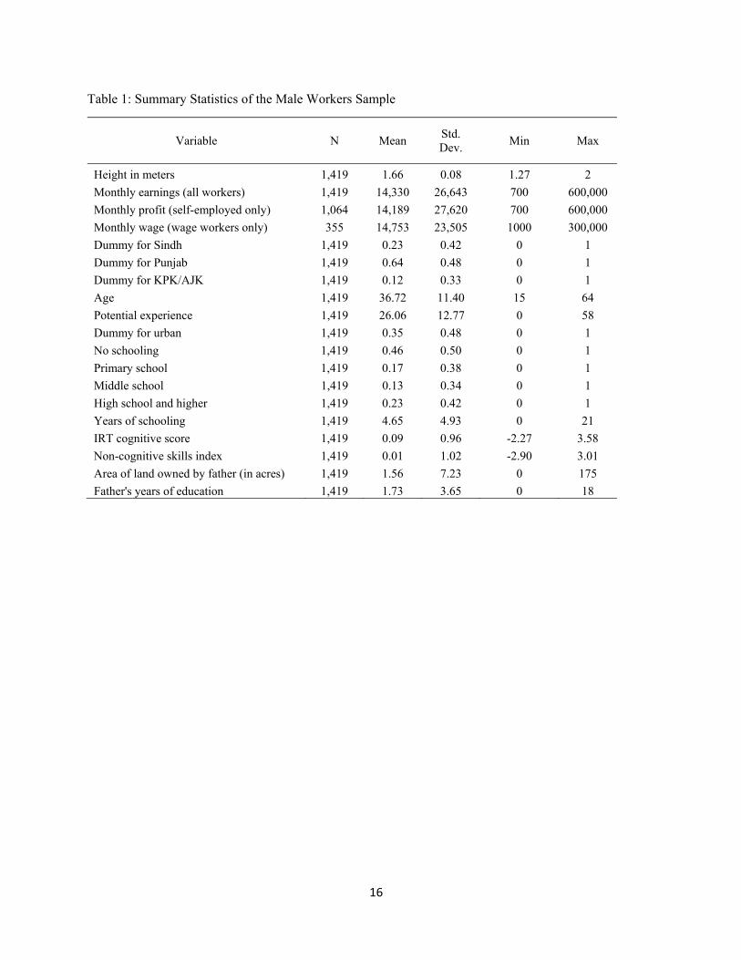
earnings for the self-employed. Table 1 reports summary statistics on this sample. There is a

legitimate concern that land owners could conflate rental earnings with crop production minus

expenses. However, this is not an obvious issue with the data. Land owners - 20% of the entire

category of self-employed and 44% of all individuals who reported cultivation as their main

employment - reported agricultural profits that were not significantly different than those reported

by renters. The median monthly profit for land-owners in the sample is PK Rps 7,000, against PK

Rps 7,500 for tenants.

Results

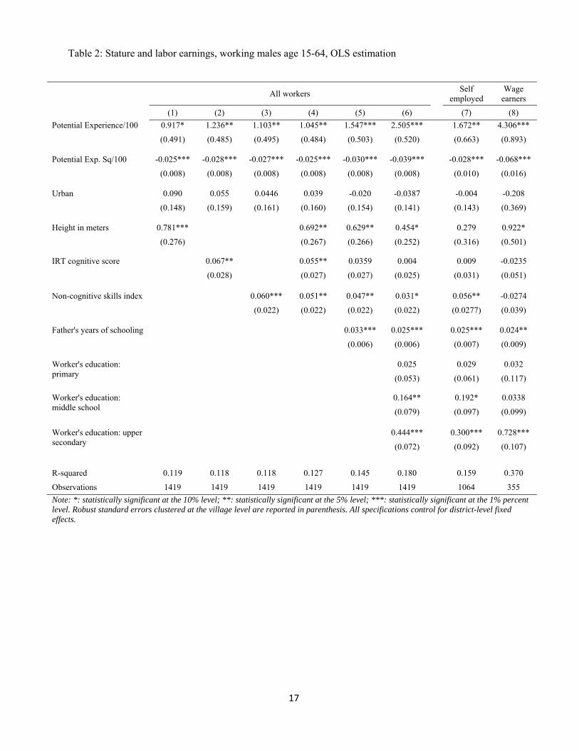
Table 2 presents OLS regressions of the logarithm of earnings from both wage and own employment.

The first three columns focus on the impacts of stature, cognitive ability and non-cognitive skills

8

entered separately. Regressions also include categorical dummies for the highest level of schooling

completed by the individual as well as potential experience and its quadratic term.4 An additional

centimeter of height contributes nearly 0.8% to earnings. The regression in the fourth column

includes all three of these measures jointly. As indicated, there is a modest attenuation of the

magnitude of height (0.7 percentage points or 11% of the initial estimate) and cognition compared

to that observed in the first three columns, but they remain individually significant.

Moreover, as shown in column 5 when we add the education of the father, that variable

proves significant. As the labor market does not directly reward the ability of the father – many of

whom are deceased - this may indicate that there are aspects of the ability of the current generation

of workers that are not directly measured by stature or the skills included here yet are recognized in

the labor market. Possibly the father’s education is a proxy for unmeasured skills that are genetically

transmitted. Alternatively, or additionally to this interpretation, the coefficient of father’s education

may indicate learning that is imparted by parental guidance. Furthermore, the coefficient can also

reflect access to networks that an educated father can facilitate. In this specification, the magnitude

of the height coefficient decreases slightly (approximately 10 percent) compared to column 4, but

remains statistically significant.

The regression in column 5 may be considered as the full reduced form impact of these

categories of skills. That is, the coefficients capture the indirect impact of these aspects of human

capital on wages via schooling and the impact of stature and skills on labor market choices regarding

sector and labor supply. In addition, they measure any direct impact on earnings conditional on these

choices. Cawley, Heckman, and Vytlacil (2001) show that the estimated impact of ability on wages

is substantially smaller when it is conditional on levels of schooling. This is also observed in our

data. Column 6 reports the impact of stature and skills conditional on schooling. The coefficient on

4 Potential experience is defined as the number of years after schooling: (age-years of schooling-6).

9

height remains significant but the magnitude declines relative to column 5. The impact of height

conditional on school might either be because it influences learning per year of school or because it

conveys abilities that are rewarded in earnings beyond the returns to schooling per se or both.

In contrast, the measure of cognitive skills is no longer significant in the regression in column

6. The standard errors for the coefficient of Raven’s declines relative to the previous estimate, so the

loss of significance is driven by the reduction of the point estimate. The impact implied by the

coefficient of Raven’s in column 5 likely works primarily through the indirect impact of skills on

schooling. That is, the coefficients in column 5 can be viewed largely as δW/δS*δS/δH. At the same

time, it appears that schooling is not merely a signal for these skills since the inclusion of schooling

increases the portion of earnings explained in the regression.

However, as mentioned, wage earnings and earnings from own employment are pooled in

the first 6 columns. Columns 7 and 8 indicate how these skills influence earnings in these two sectors

respectively. Height is far more important in wage employment than in own employment. This is in

partial contrast to Pitt, Rosenzweig, and Hassan (2013) who argue that employment in agriculture

may reflect the relative importance of physical capacity in that sector. As 41.1 percent of the

individuals in our sample who are self-employed are in agriculture the results in column 7 should

reflect the role of stature in agriculture. Our measure of socio-emotional skills is not important in

wage employment although it is in self-employment. Conditional on schooling, Raven’s scores are

not significant in either sector, although non-cognitive skills have a role in self-employment earnings

while the coefficient of father’s education is significant in both sectors.

The results in table 2, however, tacitly assume that equations 1 and 2 can be considered

lagged endogenous and also that they have no common unobservables with equation 3 and, thus, no

correlation of errors with estimations based on equation 3. We relax this assumption in table 3, which

10

reports the same regressions as in table 2 with stature instrumented.5 The land holding of the father

of the current employed individual (as this individual recollects it) is used as one of the instruments.

The first stage regression is reported in table A1 of the appendix. As the survey obtained height

information from all adults but earnings for only a subset, the full sample was used for instrumenting

height and standard errors for the second stage IV were obtained by bootstrapping rather than

running the IV estimates as a simultaneous set of equations. This approach was also motivated by

the fact that the first step of the IV corresponds to equation 1 presented in the methodology while

the wage equation is an estimate for equation 3. Time variant information that is observed at the

time of employment does not pertain to the production of skills in equation 1 and thus is not

appropriate in the estimation of height. The F statistic for the first stage regressions reported in

columns 1-4 exceeds the rule of thumb for plausible instruments from Stock and Yogo (2005).

Columns 5 and 6 offer results using an alternative instrument, the residual of a regression for

the child’s height. This residual is assumed to pick up common genetic factors as well as other

elements of the child height regression which are orthogonal to other determinants of child height.

Carslake et al. (2013) use a similar approach as an instrument for father’s height; however, in their

study, son’s height rather than a residual is employed as an instrument. As only a subset of the

sample had children who were measured, the regressions in columns 5 and 6 have fewer

observations. This has a moderate effect on the significance of the height coefficient, but the point

estimate is similar to that in columns 1 and 2. The point estimates are again similar when both

potential instruments are included in columns 7 and 8 but the standard errors increase. The

5 As columns 2 and 3 in table 2 are not affected by the IV approach used here, these are omitted in table 3.

11

regressions in those columns, however, allow an overidentification test which provides some

reassurance that the area of land owned by the father is a valid instrument.6

While the magnitude of the contribution of height to explaining wages in table 2 using OLS

regressions is somewhat lower than reported elsewhere in the literature (such as in Vogl 2014), the

magnitude of the coefficient of instrumented height in table 3 increases substantially.7 This may

reflect a combination of errors in measurement for height as well as endogenous choices. In contrast

to the OLS results the IV coefficient of height is significant for self-employed (including those

engaged in agriculture) while it is not for wage workers.

In principle, schooling is also an endogenous choice and thus it would be desirable to also

instrument the education variables in table 3. Duflo (2001), however, finds little difference between

instrumented estimates of the impact of years of schooling on wages and OLS results, a result that

reinforces an earlier review by Ashenfelter et al. (1999). Similarly, Chou et al. (2010), using an

approach similar to that of Duflo, observe little bias in the OLS coefficients on the effect of education

on birth weights and infant mortality. Thus, we assume that the results reported here are not

substantially biased by the inability to instrument education in addition to height.

The next step in this analysis concentrates on including selection into wage employment in

the determinants of earnings. The initial selection into wage employment per se is reported in table

4 while table 5 reports the results for the regressions explaining earnings conditional on this

selection. The probit equation includes land holding and education of the father of the worker as

well as a dummy variable for whether the worker’s father is still living. The probability of wage

6 In an earlier model, the Hansen’s test of over-identification indicated that father’s education was

not uncorrelated with errors in the equations reported in table 4, hence it was included in the wage

equation and not employed as an identifying instrument. 7 This was also observed by Schultz (2003) in the case of Ghana.

12

employment increases with education only when the individual has an upper secondary or higher

level of education. Conditional on education, wage employment decreases with land holding;

conversely, the probability of being self-employed including working in agriculture increases with

father’s landholding as is logical. The IRT cognitive score is significant in the choice of wage

employment even when years of completed schooling are included but neither height nor the index

of socio-emotional skills influence selection into wage employment. The absence of a role of height

in sectoral choice is in contrast to the results in both Vogl (2014) and LaFave and Thomas (2013).

However, the significance of the IRT cognitive score is consistent with other evidence in the

literature including the studies cited in the introduction.

The OLS results for wages conditional of selection reported in table 5 do not differ

appreciably from the corresponding tables which do not account for selection into wage

employment. The IV results, however, reflect the challenge of accounting for both selection as well

as endogeneity with the limited instruments for lagged decisions on health. In effect, we have to rely

on selection by functional form which is not preferred; the results can be considered indicative albeit

weakly identified. Statistical power is lost, for example, on the coefficient of height in self-

employment although the point estimate is similar to that in table 3.

Conclusion

The results reported in this paper support the view that height provides independent information on

labor productivity rather than only serving as a proxy for other common measures of human capital.

This general point is consistent with other studies that include one or more measures of skills in

addition to height. The IV results reported here also provide no indication that the association of

height and wages in OLS results is biased upwards due to unmeasured aspects of early home

environment. Moreover, the IV coefficient of height in the current study is similar in magnitude to

13

those in Schultz (2003) as well as the OLS results conditional on the inclusion of cognitive ability

in Vogl (2014). Thus, while conceptually an IV approach is preferred to OLS for measuring human

capital impacts, the results here reinforce rather than challenge the core evidence from OLS studies

in the literature.

However, drilling down a bit into the manner by which height explains labor choices

indicates that there also are some differences compared to previous studies. For example, height

seems to have no role in selection into wage work in Pakistan and, of course, given the bivariate

choice in the choice of occupations this also implies it has no role in selection into other self-

employment activities including those in which brawn is assumed to be more central.

The differences with other results in the literature likely reflect context; there are too few

studies that include both height and a range of other measures of human capital from which to

generalize. In addition, the data required for precise estimation of selection and endogenous choice

over the life-cycle are daunting. Still, given that the paper also shows that socio-emotional skills

have additional explanatory power, a finding that is more commonly noted in studies from high

income countries, the three relatively accessible measures of skills studied here confirm not only

that ability is multi-dimensional but that insights into these dimensions are available with judicious

modifications of standard labor force surveys.

14

References

Alderman, Harold, Jere Behrman, David Ross, and Richard Sabot. 1996. The Returns to Endogenous Human Capital in Pakistan's Rural Wage Labor Market. Oxford Bulletin of Economics and Statistics. 58(1): 29-55.

Ashenfelter, Orley; Harmon, Colm P. and Oosterbeek, Hessel. A Review of Estimates of the Schooling/Earnings Relationship. Labor Economics, November 1999, 6(4), pp. 453–70.

Bargain, Oliver and Jinan Zeidan. 2017. Stature, Skills and Adult Life Outcomes: Evidence from

Indonesia. Journal of Development Studies 53(6), pp.873-890. Behrman, Jere, John Hoddinott, John Maluccio, Reynaldo Martorell. 2013. Brains versus Brawn:

Labor Market Returns to Intellectual and Health Human Capital in a Poor Developing Country. Middlebury College. Dept. of Economics. Processed.

Carslake, David, Abigail Fraser, George Davey Smith, Margaret May, Tom Palmer, Jonathan

Sterne, Karri Silventoinen, Per Tynelius, Debbie A. Lawlor, and Finn Rasmussen. 2013. Associations of mortality with own height using son's height as an instrumental variable. Economics & Human Biology 11(3): 351-359.

Case, Anne and Christina Paxson. 2008. Stature and Status: Height, Ability and Labor Market Outcomes. Journal of Political Economy. 116(3): 499-532.

Cawley, John, James Heckman and Edward Vytlacil. 2001. Three Observations on Wages and Measured Cognitive Ability. Labor Economics 8:419-442.

Chou S-Y, Liu J-T, Grossman M, Joyce T. Parental education and child health: evidence from a natural experiment in Taiwan. American Economic Journal: Applied Economics 2010; 2: 33–61.

Costa, Paul and Robert McCrae. 1987. Validation of the five-factor model of personality across instruments and observers. J Pers Soc Psychol. 52(1):81-90.

Cunha, Flavio and James Heckman. 2007. The Technology of Skills Formation. American Economic Review. 2007 97(2): 31-47.

Duflo, Esther. 2001. Schooling and Labor Market Consequences of School Construction in Indonesia: Evidence from an Unusual Policy Experiment. American Economic Review 91(4): 795-813.

Haddad, Lawrence and Howarth Bouis. 1991. The impact of nutritional status on agricultural productivity: wage evidence from the Philippines. Oxford bulletin of economics and statistics, 53(1), 45-68.

Hanushek, Eric, and Ludger Woessmann. 2008. The Role of Cognitive Skills in Economic Development. Journal of Economic Literature 46 (3): 607–68.

Heckman, James, Jora Stixrud and Sergio Urzua. 2006. The Effects of Cognitive and Noncognitive Abilities on Labor Market Outcomes and Social Behavior. Journal of Labor Economics 24(3): 411-82.

15

Heckman, James and Stefano Mosso. 2014. The Economics of Human Development and Social Mobility. Annual Review of Economics, Annual Reviews 6(1): 689-733, 08.

Heckman, James and Tim Kautz. 2012. Hard evidence on soft skills. Labor Economics, 19(4): 451-464.

LaFave, Daniel and Duncan Thomas. 2017. Height and Cognition at Work. Labor Market Performance in a Low Income Setting. Economics and Human Biology. Forthcoming.

Lundborg, Petter, Paul Nystedt, and Dan-Olof Rooth. 2014. Height and earnings: The role of cognitive and noncognitive skills. Journal of Human Resources 49 (1): 141-166.

Pitt, Mark, Mark Rosenzweig, and M.N. Hassan. 2013. Human Capital Investment and the Gender

Division of Labor in a Brawn-Based Economy. American Economic Review, 102(7): 3531–60.

Schultz, Paul. 2003. Wage Rentals for Reproductive Human Capital: Evidence from Ghana and the

Ivory Coast. Economics and Human Biology. 1: 331-336. Stock, James and Motohiro Yogo. 2005. Testing for Weak Instruments in IV Regression, in

Identification and Inference for Econometric Models: A Festschrift in Honor of Thomas Rothenberg. Donald W. K. Andrews and James H. Stock, eds. Cambridge University Press, pp.80-108.

Thomas, Duncan and John Strauss, 1997: Health and Wages: Evidence on Men and Women in

Urban Brazil, Journal of Econometrics, 77(1): 159–187. Vogl, Tom. 2014. Height, Skills, and Labor Market Outcomes in Mexico. Journal of

Development Economics. 107(1): 84-96.

16

Table 1: Summary Statistics of the Male Workers Sample

Variable N Mean Std. Dev.

Min Max

Height in meters 1,419 1.66 0.08 1.27 2

Monthly earnings (all workers) 1,419 14,330 26,643 700 600,000

Monthly profit (self-employed only) 1,064 14,189 27,620 700 600,000

Monthly wage (wage workers only) 355 14,753 23,505 1000 300,000

Dummy for Sindh 1,419 0.23 0.42 0 1

Dummy for Punjab 1,419 0.64 0.48 0 1

Dummy for KPK/AJK 1,419 0.12 0.33 0 1

Age 1,419 36.72 11.40 15 64

Potential experience 1,419 26.06 12.77 0 58

Dummy for urban 1,419 0.35 0.48 0 1

No schooling 1,419 0.46 0.50 0 1

Primary school 1,419 0.17 0.38 0 1

Middle school 1,419 0.13 0.34 0 1

High school and higher 1,419 0.23 0.42 0 1

Years of schooling 1,419 4.65 4.93 0 21

IRT cognitive score 1,419 0.09 0.96 -2.27 3.58

Non-cognitive skills index 1,419 0.01 1.02 -2.90 3.01

Area of land owned by father (in acres) 1,419 1.56 7.23 0 175

Father's years of education 1,419 1.73 3.65 0 18

17

Table 2: Stature and labor earnings, working males age 15-64, OLS estimation

All workers Self employed

Wage earners

(1) (2) (3) (4) (5) (6) (7) (8)

Potential Experience/100 0.917* 1.236** 1.103** 1.045** 1.547*** 2.505***

1.672** 4.306***

(0.491) (0.485) (0.495) (0.484) (0.503) (0.520)

(0.663) (0.893)

Potential Exp. Sq/100 -0.025*** -0.028*** -0.027*** -0.025*** -0.030*** -0.039***

-0.028*** -0.068***

(0.008) (0.008) (0.008) (0.008) (0.008) (0.008)

(0.010) (0.016)

Urban 0.090 0.055 0.0446 0.039 -0.020 -0.0387

-0.004 -0.208

(0.148) (0.159) (0.161) (0.160) (0.154) (0.141)

(0.143) (0.369)

Height in meters 0.781***

0.692** 0.629** 0.454*

0.279 0.922*

(0.276)

(0.267) (0.266) (0.252)

(0.316) (0.501)

IRT cognitive score

0.067**

0.055** 0.0359 0.004

0.009 -0.0235

(0.028)

(0.027) (0.027) (0.025)

(0.031) (0.051)

Non-cognitive skills index

0.060*** 0.051** 0.047** 0.031*

0.056** -0.0274

(0.022) (0.022) (0.022) (0.022)

(0.0277) (0.039)

Father's years of schooling

0.033*** 0.025***

0.025*** 0.024**

(0.006) (0.006)

(0.007) (0.009)

Worker's education: primary

0.025

0.029 0.032

(0.053)

(0.061) (0.117)

Worker's education: middle school

0.164**

0.192* 0.0338

(0.079)

(0.097) (0.099)

Worker's education: upper secondary

0.444***

0.300*** 0.728***

(0.072)

(0.092) (0.107)

R-squared 0.119 0.118 0.118 0.127 0.145 0.180 0.159 0.370

Observations 1419 1419 1419 1419 1419 1419 1064 355

Note: *: statistically significant at the 10% level; **: statistically significant at the 5% level; ***: statistically significant at the 1% percent level. Robust standard errors clustered at the village level are reported in parenthesis. All specifications control for district-level fixed effects.

18

Table 3: Stature and labor earnings, working males age 15-64, 2 Stage Least Square Estimation

Instrument: Area of land owned by father

Instrument: Residual of child's height Both instruments

All workers Self-employed

Wage earners

All workers

All workers

(1) (2) (3) (4) (5) (6) (7) (8) Potential experience/100 0.678* 1.130 0.340 3.803**

1.706* 3.565***

2.047 3.259***

(0.410) (0.790) (0.985) (1.819)

(0.967) (1.192)

(1.374) (1.076)

Potential experience squared/100 -0.0181** -0.0211* -0.0102 -0.0601**

-0.0323** -0.0527***

-0.0383* -0.0515***

(0.00755) (0.0124) (0.0143) (0.0254)

(0.0143) (0.0170)

(0.0207) (0.0159)

Urban 0.0796 0.0579 0.0937 -0.206

0.183 0.145

0.245 0.217

(0.221) (0.203) (0.214) (0.478)

(0.209) (0.234)

(0.238) (0.239)

Height 3.228*** 2.953** 2.737** 1.284

2.910* 2.504**

2.294* 2.491

(1.146) (1.414) (1.289) (3.238)

(1.485) (1.236)

(1.345) (1.669)

IRT cognitive score 0.0214 -0.00824 -0.00359 -0.0216

0.0279 0.00130

0.0256 0.00179

(0.0270) (0.0285) (0.0338) (0.0429)

(0.0341) (0.0336)

(0.0366) (0.0307)

Non-cognitive skills index 0.0368 0.0296 0.0512* -0.0300

0.0272 0.0255

0.0336 0.0292

(0.0231) (0.0236) (0.0269) (0.0549)

(0.0352) (0.0291)

(0.0306) (0.0318)

Father's years of schooling 0.0295*** 0.0236*** 0.0238*** 0.0231**

0.0453*** 0.0425***

0.0451*** 0.0375***

(0.00660) (0.00626) (0.00786) (0.0100)

(0.00851) (0.00943)

(0.0085) (0.00923)

Worker's education: primary

0.0195 0.0196 0.0406

-0.0579

-0.0485

(0.0501) (0.0618) (0.102)

(0.0859)

(0.0715)

Worker's education: middle

0.108 0.135 0.0290

0.0983

0.0954

(0.0817) (0.123) (0.118)

(0.105)

(0.101)

Worker's education: upper secondary

0.340*** 0.199 0.703***

0.406***

0.381***

(0.0866) (0.128) (0.139)

(0.101)

(0.0972)

F-statistic of excluded instruments

14.81 11.29 8.55 10.10

22.56 22.41

27.59 24.05

F-probability of excluded instruments

0.000 0.001 0.003 0.002

0.000 0.000

0.000 0.000

Hansen J-statistic of overidentification

- - - -

- -

0.123 0.390

p-value of Hansen J statistics - - - -

- -

0.726 0.532

Number of observations 1417 1417 1060 357 838 838 810 810

Note: *: statistically significant at the 10% level; **: statistically significant at the 5% level; ***: statistically significant at the 1% percent level. Robust standard errors clustered at the village level are reported in parenthesis. All specifications control for district-level fixed effects. The F-statistic tests the hypothesis that the estimated coefficients on the instruments are zero. We use the Hansen J statistic to test for overidentification in columns (7) and (8). The total number of observations are lower in column (5) to (8) as the child's height residual instrument can only be conducted for the subsample of workers in the sample that have a child. The first stage estimation for column (5) to (8) was based on a larger sample than the second stage to increase precision, and bootstrapping was used to correct the 2SLS standard errors.

19

Table 4: Selection into Wage Employment as opposed to self-employment, working males age 15-64, Binomial Probit Estimation

Probit coefficient Marginal Effect (1) (2) (3) (4)

Potential experience/100 -4.376*** -6.665*** -1.209*** -1.062*** (1.086) (2.02) (0.292) (0.316)

Potential experience squared/100

0.042** 0.061*

0.012** 0.010*

(0.018) (0.032) (0.005) (0.005) Urban -0.286 -0.489 -0.079 -0.078

(0.341) (0.574) (0.095) (0.092) Height (in meters) -0.429 -0.865 -0.119 -0.138

(0.518) (0.901) (0.143) (0.143) IRT cognitive score 0.142*** 0.205*** 0.039*** 0.033***

(0.046) (0.078) (0.013) (0.012) Non-cognitive skills index

0.0286 0.047 0.008 0.008 (0.048) (0.0846) (0.013) (0.013)

Father's education -0.008 -0.020 -0.002 -0.003 (0.013) (0.022) (0.004) (0.004)

Primary schooling

-0.272 -0.043 (0.223) (0.036)

Middle schooling

-0.460** -0.073* (0.235) (0.038)

Upper secondary

0.389* 0.062* (0.225) (0.036)

Area of land owned by the father

-0.035** -0.066**

-0.010** -0.011**

(0.014) (0.026) (0.004) (0.004) Father is alive 0.117 -0.177 0.032 -0.028

(0.086) (0.156) (0.024) (0.025)

Number of observations 1419 1419 1419 1419 Note: *: statistically significant at the 10% level; **: statistically significant at the 5% level; ***: statistically significant at the 1% percent level. Robust standard errors clustered at the village level are reported in parenthesis. All specifications control for district-level fixed effects.

20

Table 5: Stature and labor earnings, working males age 15-64, OLS and IV estimation with 2-step Heckman selection

OLS IV (Instrument: father's land

ownership)

Self employed

Wage earners

Self employed

Wage earners

Self employed

Wage earners

Self employed

(1) (2) (3) (4) (5) (6) (7)

Potential Experience/100 0.850 3.637*** 1.690*** 4.564***

0.405 2.159 1.242*

(0.583) (1.250) (0.651) (1.004)

(0.835) (2.173) (0.729)

Potential Exp. squared/100 -0.019** -0.065*** -0.028*** -0.070***

-0.012 -0.044* -0.021*

(0.009) (0.019) (0.010) (0.016)

(0.011) (0.026) (0.011)

Urban 0.0123 -0.262 -0.004 -0.183

0.111 -0.253 0.055

(0.144) (0.485) (0.142) (0.368)

(0.177) (0.522) (0.162)

Height 0.387 1.269** 0.274 0.964**

2.456* 4.756** 1.415

(0.315) (0.493) (0.312) (0.477)

(1.364) (2.292) (1.430)

IRT cognitive score 0.0250 0.044 0.009 -0.030

0.008 0.025 0.002

(0.0301) (0.057) (0.029) (0.050)

(0.034) (0.082) (0.029)

Non-cognitive skills index 0.064** -0.0172 0.056** -0.030

0.057** -0.029 0.054**

(0.027) (0.043) (0.027) (0.038)

(0.028) (0.047) (0.027)

Father's education 0.030*** 0.035*** 0.026*** 0.025***

0.027*** 0.031*** 0.024***

(0.007) (0.009) (0.007) (0.008)

(0.007) (0.011) (0.007)

Primary schooling

0.031 0.044

0.029

(0.062) (0.116)

(0.068)

Middle schooling

0.195** 0.052

0.131

(0.098) (0.107)

(0.099)

High school or higher

0.301*** 0.711***

0.192**

(0.092) (0.103)

(0.084)

Heckman's lambda -0.028 -0.085 0.009 -0.109

-0.244 0.960*** 0.537

(0.133) (0.220) (0.102) (0.164)

(0.363) (0.086) (0.216)

F-statistic of excluded instruments

12.76 11.98 7.84

F-statistic p-value

0.001 0.001 0.004

Number of Observations 1064 355 1064 355 1064 355 1064

Note: *: statistically significant at the 10% level; **: statistically significant at the 5% level; ***: statistically significant at the 1% percent level. Robust standard errors clustered at the village level are reported in parenthesis. All specifications control for district-level fixed effects. The F-statistic tests for the IV specifications in column (4) to (8) test the hypothesis that the estimated coefficients on the instrument is zero. The Heckman’s lambda indicates the sign and statistical significance of the correlation between the error term in the Heckman selection equation and the error term in the main earnings equation.

21

Appendix: Instrumenting Equation for Endogenous Nutritional Status

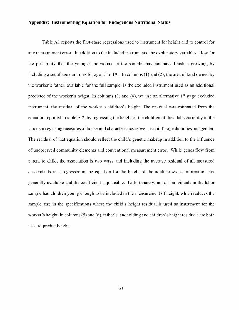
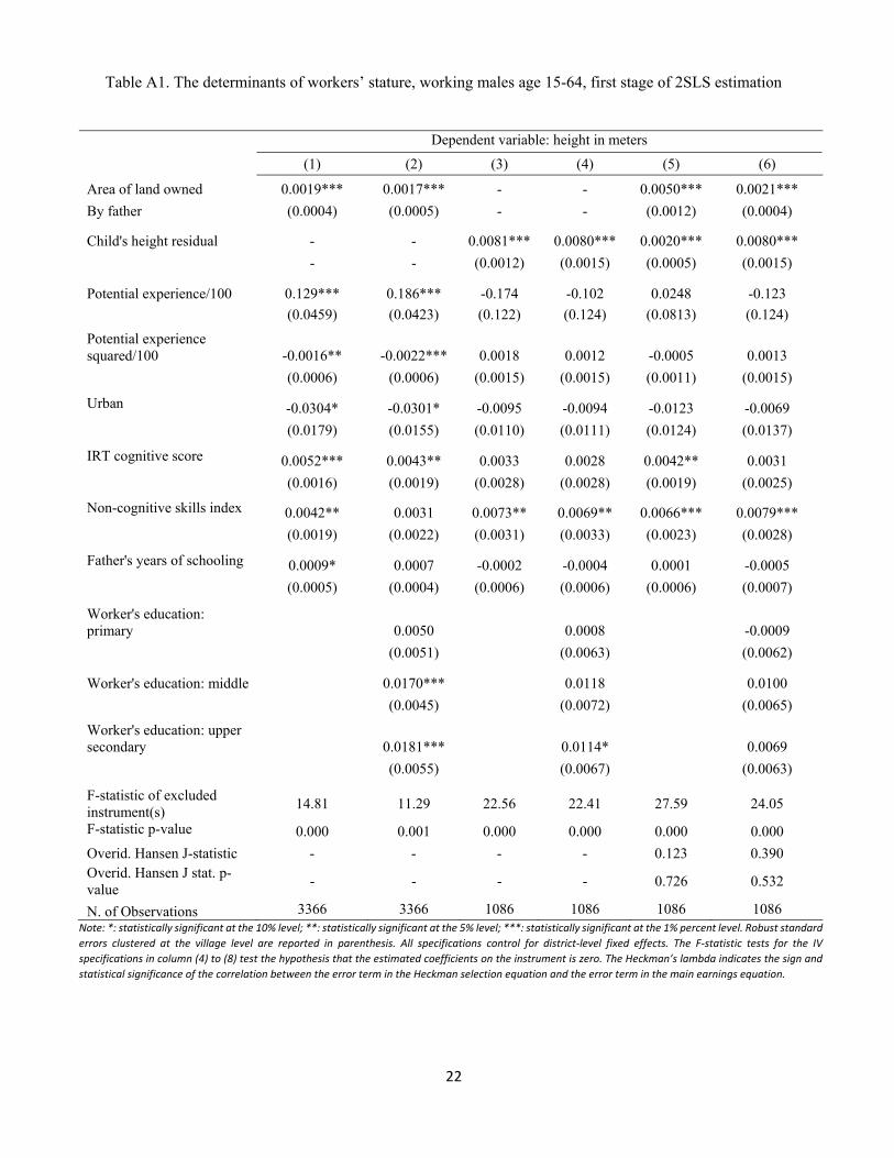
Table A1 reports the first-stage regressions used to instrument for height and to control for

any measurement error. In addition to the included instruments, the explanatory variables allow for

the possibility that the younger individuals in the sample may not have finished growing, by

including a set of age dummies for age 15 to 19. In columns (1) and (2), the area of land owned by

the worker’s father, available for the full sample, is the excluded instrument used as an additional

predictor of the worker’s height. In columns (3) and (4), we use an alternative 1st stage excluded

instrument, the residual of the worker’s children’s height. The residual was estimated from the

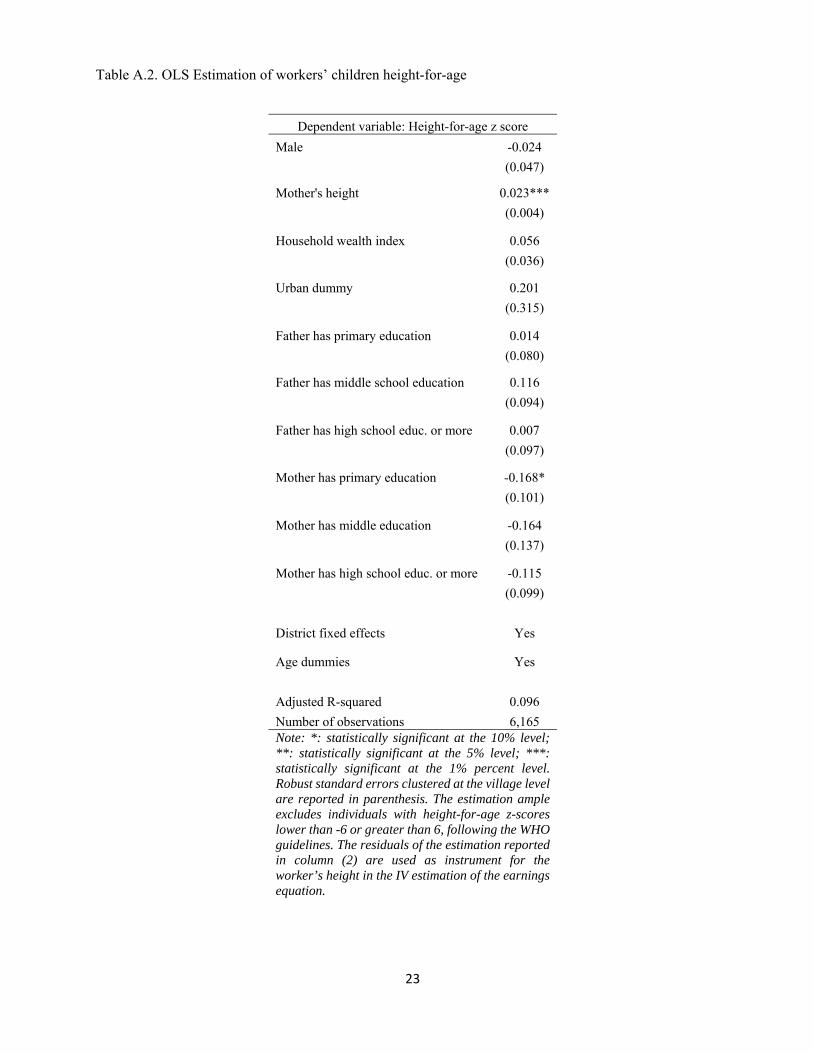
equation reported in table A.2, by regressing the height of the children of the adults currently in the

labor survey using measures of household characteristics as well as child’s age dummies and gender.

The residual of that equation should reflect the child’s genetic makeup in addition to the influence

of unobserved community elements and conventional measurement error. While genes flow from

parent to child, the association is two ways and including the average residual of all measured

descendants as a regressor in the equation for the height of the adult provides information not

generally available and the coefficient is plausible. Unfortunately, not all individuals in the labor

sample had children young enough to be included in the measurement of height, which reduces the

sample size in the specifications where the child’s height residual is used as instrument for the

worker’s height. In columns (5) and (6), father’s landholding and children’s height residuals are both

used to predict height.

22

Table A1. The determinants of workers’ stature, working males age 15-64, first stage of 2SLS estimation

Dependent variable: height in meters

(1) (2) (3) (4) (5) (6)

Area of land owned 0.0019*** 0.0017*** - - 0.0050*** 0.0021***

By father (0.0004) (0.0005) - - (0.0012) (0.0004)

Child's height residual - - 0.0081*** 0.0080*** 0.0020*** 0.0080***

- - (0.0012) (0.0015) (0.0005) (0.0015)

Potential experience/100 0.129*** 0.186*** -0.174 -0.102 0.0248 -0.123

(0.0459) (0.0423) (0.122) (0.124) (0.0813) (0.124)

Potential experience squared/100 -0.0016** -0.0022*** 0.0018 0.0012 -0.0005 0.0013

(0.0006) (0.0006) (0.0015) (0.0015) (0.0011) (0.0015)

Urban -0.0304* -0.0301* -0.0095 -0.0094 -0.0123 -0.0069

(0.0179) (0.0155) (0.0110) (0.0111) (0.0124) (0.0137)

IRT cognitive score 0.0052*** 0.0043** 0.0033 0.0028 0.0042** 0.0031

(0.0016) (0.0019) (0.0028) (0.0028) (0.0019) (0.0025) Non-cognitive skills index 0.0042** 0.0031 0.0073** 0.0069** 0.0066*** 0.0079***

(0.0019) (0.0022) (0.0031) (0.0033) (0.0023) (0.0028)

Father's years of schooling 0.0009* 0.0007 -0.0002 -0.0004 0.0001 -0.0005

(0.0005) (0.0004) (0.0006) (0.0006) (0.0006) (0.0007)

Worker's education: primary 0.0050 0.0008 -0.0009

(0.0051) (0.0063) (0.0062)

Worker's education: middle 0.0170*** 0.0118 0.0100

(0.0045) (0.0072) (0.0065)

Worker's education: upper secondary 0.0181*** 0.0114* 0.0069

(0.0055) (0.0067) (0.0063)

F-statistic of excluded instrument(s)

14.81 11.29 22.56 22.41 27.59 24.05

F-statistic p-value 0.000 0.001 0.000 0.000 0.000 0.000

Overid. Hansen J-statistic - - - - 0.123 0.390 Overid. Hansen J stat. p-value

- - - - 0.726 0.532

N. of Observations 3366 3366 1086 1086 1086 1086 Note: *: statistically significant at the 10% level; **: statistically significant at the 5% level; ***: statistically significant at the 1% percent level. Robust standard errors clustered at the village level are reported in parenthesis. All specifications control for district-level fixed effects. The F-statistic tests for the IV specifications in column (4) to (8) test the hypothesis that the estimated coefficients on the instrument is zero. The Heckman’s lambda indicates the sign and statistical significance of the correlation between the error term in the Heckman selection equation and the error term in the main earnings equation.

23

Table A.2. OLS Estimation of workers’ children height-for-age

Dependent variable: Height-for-age z score

Male -0.024

(0.047)

Mother's height 0.023***

(0.004)

Household wealth index 0.056

(0.036)

Urban dummy 0.201

(0.315)

Father has primary education 0.014

(0.080)

Father has middle school education 0.116

(0.094)

Father has high school educ. or more 0.007

(0.097)

Mother has primary education -0.168*

(0.101)

Mother has middle education -0.164

(0.137)

Mother has high school educ. or more -0.115

(0.099)

District fixed effects Yes

Age dummies Yes

Adjusted R-squared 0.096

Number of observations 6,165 Note: *: statistically significant at the 10% level; **: statistically significant at the 5% level; ***: statistically significant at the 1% percent level. Robust standard errors clustered at the village level are reported in parenthesis. The estimation ample excludes individuals with height-for-age z-scores lower than -6 or greater than 6, following the WHO guidelines. The residuals of the estimation reported in column (2) are used as instrument for the worker’s height in the IV estimation of the earnings equation.