the effect of information and communications technology (ict
TRANSCRIPT

THE EFFECT OF INFORMATION AND COMMUNICATIONS TECHNOLOGY (ICT)
DIFFUSION ON CORRUPTION AND TRANSPARENCY (A GLOBAL STUDY)
A Dissertation
by
LEEBRIAN ERNEST GASKINS
Submitted to Texas A&M International University
in partial fulfillment of the requirements
for the degree of
DOCTOR OF PHILOSOPHY
May 2013
Major Subject: International Business Administration
ii
THE EFFECT OF INFORMATION AND COMMUNICATIONS TECHNOLOGY (ICT)
DIFFUSION ON CORRUPTION AND TRANSPARENCY (A GLOBAL STUDY)
A Dissertation
By
LEEBRIAN ERNEST GASKINS
Submitted to Texas A&M International University
in partial fulfillment of the requirements
for the degree of
DOCTOR OF PHILOSOPHY
Approved as to style and content by:
Chair of Committee, Nereu F. Kock
Committee Members, Milton R. Mayfield
Andres E. Rivas-Chavez
Randel D. Brown
Chair of Department, S. Srinivasan
May 2013
Major Subject: International Business Administration

iii
ABSTRACT
The Effect of Information and Communications Technology (ICT) Diffusion on Corruption and
Transparency (A Global Study) (May 2013)
Leebrian Ernest Gaskins, MBA, West Virginia University;
Chair of Committee: Dr. Nereu F. Kock
Is the diffusion of information and communication technologies (ICTs) the “magic
bullet” for effectively reducing corruption? Can government transparency be increased by ICT
diffusion? Does ICT diffusion increase governmental transparency, thereby reducing corruption?
A few previous studies have measured the relationship between ICTs, transparency, and
corruption. Generally, such studies focus on the role of electronic governance (e-governance) in
facilitating state-citizen interactions and how e-governance acts as a corruption deterrent. This
study digresses from past literature by directly exploring the effects of the ICT environment,
using the Networked Readiness Index (NRI), and diffusion of two specific ICTs (e.g. the number
of Internet users per 100 people and mobile cellular phone users per 100 people) on corruption
and transparency through structural equation modeling.
This study also examines how macroeconomic and national sociocultural variables
mediate and moderate the relationships of ICTs on transparency and corruption. The results show
that for each increase unit in NRI, transparency increased by 9.423% and corruption decreased
by 14.017%. Furthermore, increasing access to the Internet by 27 people per 100 persons
increased transparency by 17.581% and reduced corruption by 15.239%. Additionally, each unit

iv
increase in per capita GDP results in an increase in transparency by 7.068% and a decrease in
corruption by 10.507%. Conversely, increases in FDI and mobile cellular diffusion demonstrated
marginal results on increasing transparency and reducing corruption. Implications of these
findings as well as avenues for further research are discussed.

v
ACKNOWLEDGEMENTS
I wish to express my deepest gratitude and appreciation to my advisor, mentor, and
committee chair, Dr. Nereu F. Kock. He has provided me with invaluable personal and
professional guidance. To my dissertation committee—Drs. Milton R. Mayfield, Andres E.
Rivas-Chavez, and Randel D. Brown—thank you for the wealth of knowledge, advice,
encouragement and support you have provided throughout this process.
My doctoral endeavors would not have been possible without special people supporting
me along the way. Thanks to Dr. Ray M. Keck, III and Juan J. Castillo who encouraged me to
pursue my doctorate and made it all possible. Thanks to the staff of the Office of Information
Technology. I would like to give special thanks to Yezmin Salazar, Mario Peña, Jackie
Rodriguez, Pablo Reyes-Soriaña, Dr. Patricia Abrego, Claudia Escobar, and Cuauhtémoc
Barrios. Their hard work in the Office of Information Technology combined with words of
encouragement made it possible for me to be a successful Chief Information Officer and doctoral
student.
A special thank you to all of my fellow doctoral students who provided support,
friendship, advice and help throughout the program. Finally, I wish to thank my family for their
love, sacrifice, encouragement and support.

vi
TABLE OF CONTENTS
ABSTRACT ........................................................................................................................ iii
ACKNOWLEDGEMENTS ............................................................................................... v
TABLE OF CONTENTS ................................................................................................... vi
LIST OF TABLES ............................................................................................................. viii
LIST OF FIGURES ............................................................................................................ x
I. INTRODUCTION ........................................................................................................... 1
1.1 Overview ........................................................................................................... 1
1.2 Research Question ............................................................................................ 4
1.3 Significance and Purpose of Study ................................................................... 5
II. REVIEW OF THE LITERATURE ................................................................................ 7
2.1 Corruption ......................................................................................................... 7
2.2 Information and Communication Technologies and Corruption ...................... 22
2.3 Research Hypotheses ........................................................................................ 25
2.4 Theoretical Model ............................................................................................. 32
III. METHODOLOGY ....................................................................................................... 35
3.1 Sample Design .................................................................................................. 35
3.2 Data Collection ................................................................................................. 37
3.3 Variable Description ......................................................................................... 38
3.4 Data Preparation................................................................................................ 48
3.5 Data Validation ................................................................................................. 60
3.6 Data Analysis .................................................................................................... 69

vii
IV. RESULTS ..................................................................................................................... 74
4.1 Descriptive Statistics Analysis .......................................................................... 74
4.2 Structural Model Analysis ................................................................................ 88
4.3 Model Fit Indices .............................................................................................. 94
4.4 Hypotheses Testing ........................................................................................... 96
4.4 Direct, Indirect and Total Effects ...................................................................... 107
V. DISCUSSION ................................................................................................................ 128
5.1 Overview of the Study ...................................................................................... 128
5.2 Overview of Findings ....................................................................................... 132
5.2.1 Macroeconomic Variable Findings .................................................... 132
5.2.2 ICT Variable Findings ....................................................................... 136
5.2.3 Control Variable Findings.................................................................. 138
5.2.4 Transparency’s effect on Corruption ................................................. 140
VI. CONCLUSION............................................................................................................. 141
6.1 Summary ........................................................................................................... 141
6.2 Limitations ........................................................................................................ 148
6.3 Implications and Future Research ..................................................................... 149
6.4 Conclusion ........................................................................................................ 151
REFERENCES ................................................................................................................... 153
VITA ................................................................................................................................ 181
viii
LIST OF TABLES
Table 3-1. List of countries used in this study. ................................................................... 36
Table 3-2. Data sources for variables. ................................................................................ 37
Table 3-3. Number of data items collected for each variable by year. ............................... 38
Table 3-4. Voice and Accountability (VA) indicator data types and sources. ................... 44
Table 3-5. Percentage of missing data values by variable (N=605). .................................. 49
Table 3-6. Results of normal distribution test on Hofstede data. ........................................ 53
Table 3-7. Missing data percentages after listwise deletion (N=461). ............................... 56
Table 3-8. United Nations geoscheme regions (with area codes). ...................................... 58
Table 3-9. Missing data percentages after regional mean substitution (N=605). ............... 59
Table 3-10. Correlation matrix for RMS treated data. ........................................................ 63
Table 3-11. Correlation matrix for LD treated data. .......................................................... 64
Table 3-12. Variance inflation factors by variable and missing data treatment. ................ 65
Table 3-13. Block VIF values using RMS. ......................................................................... 67
Table 3-14. Block VIF using LD. ....................................................................................... 68
Table 3-15. Stone-Geisser Q-squared coefficients. ............................................................ 69
Table 4-1. Descriptive statistics of data using LD. ............................................................. 75
Table 4-2. Descriptive statistics of data using RMS. .......................................................... 76
Table 4-3. Descriptive statistics of the data. ...................................................................... 77
Table 4-4. Number of significant paths by P-value level. ................................................. 94
Table 4-5. Model fit indices with associated P-values. ...................................................... 95
Table 4-6: Summary results of hypotheses testing ............................................................. 96
Table 4-7. Direct effects for each variable relationship. ..................................................... 110

ix
Table 4-8. Indirect effects for relationships with two aggregated segments. ..................... 111
Table 4-9. Indirect effects for relationships with three aggregated segments. ................... 114
Table 4-10. Indirect effects for relationships with four aggregated segments. ................... 116
Table 4-11. Indirect effects for relationships with five aggregated segments. ................... 118
Table 4-12. Sum of indirect effects..................................................................................... 119
Table 4-13. Total effect of FDI. .......................................................................................... 123
Table 4-14. Total effect of GDP per capita......................................................................... 124
Table 4-15. Total effect of NRI. ......................................................................................... 125
Table 4-16. Total effect of Internet diffusion. .................................................................... 125
Table 4-17. Total effect of Mobile diffusion. ..................................................................... 126
Table 4-18. Total effect size of Transparency. ................................................................... 126

x
LIST OF FIGURES
Figure 2-1. Theoretical model with hypotheses and predicted effects. .............................. 34
Figure 4-1. Structural model with RMS and bootstrapping. ............................................... 90
Figure 4-2. Structural model with RMS and jackknifing. ................................................. 91
Figure 4-3. Structural model with LD and bootstrapping. ................................................. 92
Figure 4-4. Structural model with LD and jackknifing. ..................................................... 93
Figure 4-5. Relationship between FDI and NRI. ................................................................ 97
Figure 4-6. Relationship between GDP per capita and NRI ............................................... 98
Figure 4-7. Relationship between NRI and Internet diffusion. ........................................... 99
Figure 4-8. Relationship between NRI and Mobile diffusion............................................. 100
Figure 4-9. Relationship between Mobile and Internet diffusion. ...................................... 101
Figure 4-10. Relationship between Internet diffusion and transparency. ........................... 102
Figure 4-11. Relationship between mobile diffusion and transparency. ............................ 103
Figure 4-12. Relationship between Internet diffusion and corruption. ............................... 104
Figure 4-13. Relationship between transparency and corruption. ...................................... 105
Figure 4-14. Relationship between mobile diffusion and corruption. ................................ 106

1
This dissertation follows the style of the Journal of Information Technology for Development.
CHAPTER I
INTRODUCTION
1.1 Overview
Corruption, along with possible remedies and measures for fighting corruption, has been
studied academically in a multitude of ways over the past sixty years (Akçay, 2006; Arvas &
Ata, 2011; Donchev & Ujhelyi, 2009; Leff, 1964; Macrae, 1982; Mauro, 1995; McMullan, 1961;
Myrdal, 1970a; Nye, 1967; Rose-Ackerman, 1978, 1999, 2008; Svensson, 2005). The wide-
ranging definition used by the World Bank, Transparency International, and most scholars is that
corruption is the abuse of public power for private benefit or profit (Amundsen, 1999; Andvig,
Fjeldstad, Amundsen, Sissener, & Søreide, 2000; Gray & Kaufmann, 1998; Rose-Ackerman,
1996). Corruption, as similarly addressed in this paper, is the use of public office or power for
personal gain. In its many forms, corruption leads to the misallocation of public resources,
thereby creating bias against efficient projects and practices (Macrae, 1982).
Corrupt practices not only make public power and governance less efficient, such as the
management of public resources, but they also adversely affect countries’ competitiveness and
human development (Akçay, 2006). Studies have shown that the effect of corruption on human
development is more evident in some countries than others (Waheeduzzaman, 2005). In some
countries, for instance, high levels of corruption reduce the productivity of public sector
investments (Tanzi, 1995). International investment such as Foreign Direct Investment (FDI)
into countries perceived as “corrupt” is substantially less than in countries without this
perception (Habib & Zurawicki, 2002). Countries with higher levels of corruption suffer from
less than optimal economic development (Cuervo-Cazurra, 2008; Habib & Zurawicki, 2002;
Wei, 2000). Corruption has a profound mitigating effect on economic development variables

2
such as Gross Domestic Product (GDP) per capita. Mauro (1995) found that the reduction of
corruption is associated with a significant increase in GDP per capita. This finding is quite
important as GDP per capita is one of the most widely used macroeconomic indicators of a
country’s standard of living (Ringen, 1991). Similarly, as corruption increases, personal income
decreases (Alam, 1995; Husted, 1999).
The literature cited above demonstrates that corruption has a diminishing effect on
macroeconomic variables. Corruption’s effect on macroeconomic variables such as FDI and
GDP per capita is particularly important since macroeconomic and technology development
variables are interrelated. For example, there is evidence that FDI impacts information and
communication technologies (ICTs) proliferation and development (Baliamoune-Lutz, 2003;
Gholami, Lee, & Heshmati, 2006; Suh & Khan, 2003). Specifically, Lee, Gholami, and Tong
(2005) demonstrated a dual causal relationship between investments in ICT and inflows of FDI.
In the study by Lee et al. (2005), the dual causality relationship suggested that increased FDI
inflows positively affected ICT investment and proliferation, and ICT investment and
proliferation attracted more FDI inflows. There is reason to believe that any variable affecting
FDI inflow would, in turn, affect ICT development. For example, FDI is substantially less in
countries perceived as “more corrupt” (Campos, Lien, & Pradhan, 1999; Habib & Zurawicki,
2002). Therefore, countries perceived as corrupt would have substantially less FDI inflows.
These reduced FDI inflows also would negatively affect ICT investment and proliferation.
A greater percentage of the world’s population now has availability and access to ICTs
such as Internet and mobile cellular technologies (Haddon, 2004). This increased availability of
ICTs has inspired researchers to look into ways such technologies can improve economic and
human development (Gascó-Hernández, Equiza-López, & Acevedo-Ruiz, 2007; Rahman, 2007).
3
Access to mobile communications and the Internet has enabled citizens to participate more
directly in the political and social institutions and environment of their countries. Citizens are
interacting more directly with their governments, elected officials, and other citizens through
such means as e-governance (M. Backus, 2001), online political activism (Hill & Hughes, 1998),
Internet political mobilization (Krueger, 2006), and online information gathering about political
issues (Krueger, 2002).
Since corruption negatively affects economic and human development, ICTs have
fostered academic interest as a tool in reducing corruption and increasing democracy (Soper,
2007). The Internet’s potential for reducing corruption is “promising and obviously vast” (Vinod,
1999, p. 10). Past studies have examined the effects of e-governance on corruption (Hoque,
2005; Pathak & Prasad, 2005; Pathak, Singh, Belwal, Naz, & Smith, 2008; Pathak, Singh,
Belwal, & Smith, 2007) and the effects of e-governance and social media on transparency
(Bertot, Jaeger, & Grimes, 2010). These studies suggest that increased access to information
through ICTs has a positive effect on transparency and reduces corruption.
While governments and scholars are researching ways to fight corruption, ordinary
individuals armed with access to cellular phones, personal computers, and the Internet have
begun a wave of participatory journalism targeted at corruption in society (Katz & Lai, 2009).
For example, in Goa, India, an anonymous citizen uploaded to the Internet an eight-minute video
of a drug dealer talking about his connections to high-ranking anti-narcotic police (MSNIndia,
2010). In Kenya, citizens have caught and filmed traffic cops collecting bribes from motorists
(NTV, 2010). In the case of India and Kenya, citizens are acting as anti-corruption agents by
bringing corrupt practices and officials into public awareness. Such cases illustrate that citizens
have taken on the role of government in fighting corruption. Likewise, Hay and Shleifer (1998)

4
found that in the absence of strong governmental anti-corruption efforts, private enforcement by
citizens becomes a surrogate for public justice.
Vinod (1999) stated that increasing education and expanding economic freedoms are
among the top actions in reducing corruption. ICT promotes greater governmental transparency
by removing information barriers and asymmetry (Sturges, 2004). Mobile technologies and
Internet access enables citizens to become more informed with relevant information about their
government and society. The access and expansion of relevant information concerning
governmental issues promotes greater transparency (García-Murillo, 2010). Also, the diffusion
of ICTs has been shown to foster civil and political freedoms (Baliamoune-Lutz, 2003).
The diffusion of ICT affords citizens increased networking capacity and political
awareness while reducing information transaction costs (Pirannejad, 2011). Usage of ICTs to
organize, communicate, and raise awareness have been seen in such movements as the Arab
world’s “Arab Spring” and Mexico’s narcobloggers (Hofheinz, 2005; Shirk, 2010). In countries
such as India, Kenya, and Mexico, citizens are using ICTs to expose and fight governmental
corruption and civilian crime (M. Backus, 2001). Indeed, Soper (2007) demonstrated that a
negative relationship exists between investment in ICT and political corruption levels in
emerging economies.
1.2 Research Question
Some previous studies have examined the relationship between ICTs and corruption.
Such studies have focused on the role of e-governance facilitating state-citizen interactions,
thereby increasing governmental accountability and transparency (Andersen et al., 2010; M.
Backus, 2001; Bertot et al., 2010; Pathak et al., 2008; Shim & Eom, 2009) and how ICTs can

5
improve economic and human development by reducing information asymmetry (Forestier,
Grace, & Kenny, 2002; Gascó-Hernández et al., 2007; Opoku-Mensah, 2000; Rahman, 2007).
No research has yet examined if the relationship between the ICT environment, diffusion
of specific ICTs, and the two macroeconomic variables of FDI and Gross Domestic Product
(GDP) per capita has any potential effects on increasing transparency and reducing corruption.
Therefore, this study attempts to fill a gap in the literature by directly examining the effects of
the relationship of the ICT environment, diffusion of specific ICTs, FDI and GDP per capita on
corruption and transparency through structural equation modeling.
1.3 Significance and Purpose of Study
Research on how ICT diffusion and environment can be used to increase governmental
transparency and reduce corruption is important for several reasons. First, as suggested by Soper
(2007), research into using ICTs to increase transparency and reduce corruption provides the
“best scientific advice possible to world leaders who are seeking to lift their citizens…”(p. 8).
ICTs have the ability to support the free exchange of information, thereby informing citizens
about their government and society. ICTs promote greater transparency by removing information
barriers and asymmetry (Sturges, 2004) and fostering civil and political freedoms (Baliamoune-
Lutz, 2003). Indeed, there is a trend in many developed countries towards publishing information
on the Internet concerning governmental issues (García-Murillo, 2010).
Secondly, the ability of ICTs to reduce corruption can expand economic freedom. As
Vinod (1999) stated, increasing economic freedom and education is among the top actions in
reducing corruption. There is less than optimal economic development in countries with higher
levels of corruption (Cuervo-Cazurra, 2008; Habib & Zurawicki, 2002; Wei, 2000). Also,

6
corruption reduces economic freedoms by placing a burden on the economy. Every dollar worth
of corruption in developing countries, when viewed as a form of illegal taxation, equates to $1.67
worth of economic burden (Vinod, 1999). The economic burden of corruption in developing
countries compounds over time and is more distortionary than actual taxes (Vinod, 1999).
Therefore, a reduction of corruption would have a significant impact in the reduction of
economic disparity.
The purpose of this study is to do as Pirannejad (2011) suggests: future research on how
specific ICTs affect political development, especially in the context of how people monitor and
hold their government accountable. First, this study attempts to fill a gap in the existing research
advocated by Pirannejad (2011) by investigating the effects of the ICT environment and the
diffusion of two specific ICTs on corruption and transparency. Secondly, this study sets forth a
robust path model of the ICT environment, the diffusion of two specific ICTs, and two
macroeconomic variables to examine the relationship among ICTs and macroeconomic variables
in providing greater government transparency and reducing corruption. As of yet, no other
research has examined such a relationship using a robust path modeling. Therefore, this study
attempts to provide a significant contribution to the existing body of research by investigating the
effect of the ICT environment and the diffusion of two specific ICTs on corruption and
transparency in the context of two macroeconomic variables.

7
CHAPTER II
REVIEW OF THE LITERATURE
2.1 Corruption
Corruption has been a topic for writers and scholars since antiquity. The writer of the
Arthashastra, an ancient Indian text written around 4 BCE, talks about the eventuality of
corruption and the need to minimize it (Kautalya & Rangarajan, 1992). The academic study of
corruption has been explored in several different ways over the past sixty years in international
business, economics, and political science literature (Akçay, 2006; Arvas & Ata, 2011; Donchev
& Ujhelyi, 2009; Leff, 1964; Macrae, 1982; Mauro, 1995; McMullan, 1961; Myrdal, 1970a;
Nye, 1967; Rose-Ackerman, 1978, 1999, 2008). Such explorations on the topic of corruption
have included: what corruption is, what the different types of corruption are, how corruption
affect governments and their citizenry, and possible anti-corruption remedies and measures.
According to Myrdal (1970a), sparse serious academic attention was given to the topic of
corruption prior to his seminal works as the topic was considered “taboo” (p. 227). Myrdal
(1970a) suggested that empirical research should be done to “establish the general nature and
extent of corruption… and any trends that are discernible” (p. 231). Earlier examination into
systemic corruption focused on the moral, cultural, and historical causes and effects of
corruption, while later studies began to examine institutional and political aspects of corruption
(Galtung & Pope, 1999).
Several researchers have previously undertaken the task of defining corruption such as
Myrdal (1970a), Heidenheimer (1970), Rose-Ackerman (1978), Macrae (1982), Colander
(1984), and Ades and Di Tella (1999). Most authors admit that defining and conceptualizing

8
corruption is difficult, thereby hindering research in the area (Farrales, 2005; Peters & Welch,
1978). There are a wide range of activities described in the research literature that can be
classified as corrupt practices, from advantageous influence over and lobbying on government
and political agents, to outright illegal activities such as bribery, extortion, and fraud.
Furthermore, operationalizing corruption has proven difficult since corrupt behavior does not
lend itself to direct, unbiased, and measurable observation (Andvig et al., 2000). Rose-Ackerman
(1978) stated that corruption must be examined using political science and modern economics.
This approach combines the economist’s models of self-interested behavior with the political
scientist’s understanding of bureaucratic incentive structures.
Rose-Ackerman (1978) examined corruption through extending the principal-agent
model found in the economics and political science research literature. The principal-agent
model arises from the division of labor and exchange (Smith, 1776). The principal is someone
who wishes for some action to be done but cannot or does not perform the action. The principal
enlists the services of the agent to perform the desired action on the principal’s behalf (Laffont,
2003). In political science, the principal consists of voters who enlist elected officials as agents
to govern on the electorate’s behalf. In the Rose-Ackerman (1978) principal-agent model,
corruption is primarily bribery of an agent who is an elected or appointed official. The principal
of this agent is the electorate or some supervisor who specifies desired outcomes. As monitoring
of the agent is costly, in terms of time and resources, the agent has some freedom to place his
own interest above that of the principal. A third person who can benefit from the agent’s action
or inaction offers the agent an incentive (e.g. a bribe) to influence his actions. The benefits of
these incentives are not usually passed on to the principal. These incentives do not necessarily
9
subvert the principal’s objectives, and in some cases, the principal may be more satisfied with
the agent’s performance.
Another relevant model of corruption is that of Macrae (1982) in which corruption is
defined as an “arrangement” (p. 678) involving “a private exchange between two parties (the
‘demander’ and the ‘supplier’), which (1) has an influence on the allocation of resources either
immediately or in the future, and (2) involves the use or abuse of public or collective
responsibility for private ends” (p. 678). Thus, corruption is the use of public office or power for
personal gain. In contrast to the Rose-Ackerman (1978) model, which examines corruption
through the principal-agent problem, Macrae (1982)’s model of corruption explores a supply and
demand relationship for the reallocation of public resources for private gain. Hence, corruption
allows the misallocation of public resources, thereby creating bias against technological
advances and efficient projects and practices (Mauro, 1995).
Corruption, according to Myrdal (1970a), has one defining aspect being the “difference in
mores as to where, when, and how to make personal gain” (p. 233). Myrdal (1970a) further states
that corruption introduces “irrationality” (p. 233) in government planning and fulfillment. Such
irrationality influences development in such a way as to deviate from the intended plan and
fulfillment for personal gain. Corruption, thereby, hampers the decision-making and execution
processes at all levels of government (Myrdal, 1970a). Nye (1967) defined corruption as
“behavior [that] deviates from the formal duties of a public role of private-regarding …
pecuniary or status gains; or violates rules against the exercise of certain types of private-
regarding influence” (p. 416). Nye (1967)’s definition speaks of formal rules and duties and is
expansive, including such practices as nepotism, misappropriation, conflicts of interest, and
bribery.

10
A widely utilized definition of corruption put forth by Heidenheimer, Johnston, and Le
Vine (1989) and Rose-Ackerman (1978) is that corruption is a transactional relationship between
public and private sector agents by which collective goods or services are converted
(illegitimately) into private gains. Scholars in the study of corruption focus on one of two types
of corruption: bureaucratic or political (Farrales, 2005). Furthermore, Huntington (1968a) posed
that political corruption can exist in two forms. Some scholars propose that any valid assessment
of corruption must include political dimensions (Hope & Chikulo, 2000; Johnston, 1997).
Political corruption is generally viewed as the practice of using wealth, power, or status to
influence the political system in order to gain political advantage. Conversely, another form of
political corruption is when politicians use political influence and advantage to gain private
wealth, power, or status. Political corruption usually takes place with highly placed or elected
officials and is furthered by policy or legislation formation tailored to benefit the corrupt officials
(Moody-Stuart, 1997). Bureaucratic corruption is the corrupt behavior in the administration of
public policy. It seeks to influence governmental processes, such as obtaining permits or
avoiding tariffs, or paying government enforcement officials.
Corruption can also be defined in economic and social terms. Economic corruption
involves the exchange of tangible goods in a market-like situation such as bribes or rent-seeking
(Andvig et al., 2000). Rent-seeking is often classified as a type of economic corruption. This
type of corruption involves misuse of public power to derive excess earnings by the elimination
of competition (Ades & Di Tella, 1999). Rent-seeking is not necessarily banned by legislation or
shunned by society’s moral obligation. However, it reduces public wealth in favor of private gain
and generally proves economically wasteful and inefficient (Coolidge & Rose-Ackerman, 2000).
Social corruption is understood best as an integrated part of clientelism, nepotism, class or group

11
favoritism. In such social corruption, there is an exchange of material benefit based on some
criteria having a large social or cultural implication (Briquet & Sawicki, 1998).
Amundsen (1999) put forth five main manifestations of corruption: bribery,
embezzlement, fraud, extortion, and favoritism. The first and most quintessential manifestation
of corruption is bribery. Bribery is a payment, usually to a government official, to receive some
governmental benefit. Bribery has many effective forms such as kickbacks and pay-offs. The
second manifestation of corruption is embezzlement. While embezzlement is not strict
corruption, its practice deprives the government of funds. It is similar to bribery except that it
typically does not involve the private sector. The third manifestation of corruption is fraud. This
type of corruption involves the manipulation or distortion of information or fact by public
officials. Fraud, similar to the Rose-Ackerman (1978) principal-agent model, involves an agent
(e.g. public official) who carries out the directives of his principals (e.g. supervisors). The agent
manipulates the flow of information for some illegal gain that may or may not benefit the
principal (Eskeland, Thiele, & World Bank, 1999). The fourth type of corruption manifestation is
extortion. Similar to bribery, this method extracts benefits by way of coercion, violence, or threat
of force. Bribery and extortion are equivalent to extra taxes levied by – but not collected for – the
government (Wei, 1997). The fifth manifestation of corruption is favoritism. This mechanism of
corruption allows the differential access to governmental power or state resources regardless of
merit. This method of corrupt behavior can be examined as enfranchising (e.g. preferential
treatment, cronyism, and nepotism) or disenfranchising (e.g. discrimination) based on some
criteria having a large social or cultural implication (Briquet & Sawicki, 1998).
The wide-ranging definition used by the World Bank, Transparency International and
most scholars is that corruption is the abuse of public power for private benefit or profit
12
(Amundsen, 1999; Andvig et al., 2000; Gray & Kaufmann, 1998; Rose-Ackerman, 1996). Most
literature examines governmental corruption, which is the relationship between the public and
private entities engaged in corrupt behaviors. However, there exists corruption among private
businesses and non-governmental organizations (Andvig et al., 2000). This private sector
corruption exists with or without the involvement of a government official or political advantage.
Corruption is difficult to measure directly. Peters and Welch (1978) and Farrales (2005)
noted that defining and conceptualizing corruption is difficult, thus hindering research in the
area. There are a multitude of activities that can be classified as corrupt practices which makes
operationalizing of corruption difficult. Corrupt practices would have to be measured by an
unbiased observer familiar with rules and policies in a given context. Most corrupt behavior does
not lend itself to such direct, unbiased, and measurable observation (Andvig et al., 2000).
One observable measure of corruption is court cases. Such judiciary data on corruption is
collected on an international basis by the United Nations’ Crime Prevention and Criminal Justice
Division (United Nations, 1999). In such court cases, legal officials determine whether
transactions or exchanges were actually corrupt. While court cases can provide an observable
measure, Andvig et al. (2000) pointed out several issues with using such observations. First,
using such court cases as an indication or prevalence of corruption relies on the honesty of the
local judiciaries. Intraregional and international differences obviously exist in the honesty of
judiciaries which make such observations problematic in a cross-country analysis. Secondly,
local policing, judicial and political priorities usually determine which cases are prosecuted. Goel
and Nelson (1998) suggest that court cases on corruption represent more of the judicial
efficiency rather than corruption prevalence in a country. Police and other investigatory agencies
reporting on corruption provide an additional observable measure of corruption. The quality of

13
information from such agencies, however, is quite inconsistent and biased (Andvig, 1995;
Duyne, 1996).
News reports and other investigative journalistic methods are another way to measure and
fight corruption (Reinikka & Svensson, 2005). However, using such news reports and
investigative journalism as an observable measure of corruption is problematic. News and media
reports of corruption can show bias in a similar fashion to court cases and policing reports.
Media and news reports tend to give priority to high-profile or sensational cases. This selective
priority creates a bias that may not examine or expose the more pervasive everyday corrupt
activities. Furthermore, reported stories often are a factor of press freedom which are not uniform
among countries (Nixon, 1960). Therefore, the effectiveness of a free press on reducing
corruption largely relies on the measure of press freedom (Brunetti & Weder, 2003). Also, public
exposure of corruption and crime can be dangerous for the reporting journalists (Archibold,
2012). Corrupt and criminal officials typically do not care for such negative exposure due to
repercussions from law enforcement or other criminal elements. Sources of corruption are
strongly influenced by such biases as media attention, public opinion, and press freedom, making
it difficult to use such stories in a cross-country comparison.
Though corruption is difficult to define, conceptualize, and operationalize (Farrales,
2005; Peters & Welch, 1978), there have been attempts to develop an empirical measure of
corruption. These attempts to develop an empirical measure of corruption as based on the
perception of corruption rather than the actual instances or experiences of corruption. There is
some academic debate on whether a perception-based measure can adequately compare to an
experience-based measure (Donchev & Ujhelyi, 2009; Kaufmann, Kraay, & Mastruzzi, 2007,

14
2010). However, the indices listed below became the de facto empirical measures of corruption
used in academic research (Lambsdorff, 1999a; Lancaster & Montinola, 1997).
Business International Corporation (BI) created one of the first corruption perception
measurements. BI was a business advisory firm founded in 1953 which assisted American
companies in foreign business operations. BI surveyed its network of international
businesspeople, journalists, and country specialists, determining whether or not and to what
extent businesses were engaged in corruption transactions. BI also gathered survey data on such
factors as political risk, commercial hazard, and level of corruption in various countries. This
perceived level of corruption was measured on a scale from 0 to 10. BI undertook efforts to make
ranks consistent among respondents. Using the BI data for fifty-two countries, Mauro (1995)
conducted the first quantitative study of corruption using an econometric model. Mauro (1995)’s
study examined the effect of corruption on the economic growth rate. As a result, Mauro (1995)
found that corruption lowered investment, which in turn lowered economic growth.
The International Country Risk Guide (ICRG) contains another well-known corruption
perception measurement. The ICRG has been published since 1980, making it the longest
country risk analysis dataset. The ICRG measures several country factors, but the one most
related to corruption is the ICRG bureaucratic quality scale. The scale measures expert opinions,
from 1 to 6, and shows how efficiently and predictable bureaucrats operate (S. Johnson,
Kaufmann, & Zoido-Lobatón, 1998). The ICRG is published by the Political Risk Services
Group and provides a monthly political, economic, and financial risk ranking for 140 countries.
The Political Risk Services Group, founded in 1979, is one of the earliest commercial providers
of political and country risk data to companies doing international business. The ICRG also

15
contains the rule-of-law scale, from 0 to 6, measuring the strength and application of law and
order in the country.
Arguably the most well-known and widely-used index of corruption is the Corruption
Perception Index (CPI) by Transparency International (TI) which is an international non-
governmental organization founded in 1993 that monitors and reports on political and corporate
corruption in international development (Andvig et al., 2000; Brown, 2006; De Maria, 2008;
Lambsdorff, 1999b; Svensson, 2005). The CPI measures the perceived degree of corruption that
exists among public officials and politicians (Lambsdorff, 1999a). The CPI is the most widely
disseminated and popular index among policymakers. It is a composite index including survey
data from country experts, businesspeople, global analysts, and experts who are residents of the
evaluated countries (Svensson, 2005). The CPI focuses on perceptions of public sector
corruption. This index ranks countries on a scale from 10 (representing a very clean/very little
corruption government) to 0 (representing a highly corrupt government). TI uses 17 different
surveys and polls from 10 independent organizations: Freedom House (FH); Gallup International
(GI); The Economist Intelligence Unit (EIU); Institute of Management Development (IMD);
International Working Group (developing the Crime Victim Survey); Political and Economic
Risk Consultancy (PERC); Political Risk Service (PRS); The Wall Street Journal - Central
European Economic Review (CEER); World Bank and University of Basel (WB/UB); and
World Economic Forum (WEF). The CPI is widely-used as there is a high degree of correlation
between the 17 polls and surveys used (Lambsdorff, 1999a). The use of several different survey
instruments and the high inter-correlation between instruments results provide a major strength
to the CPI. The surveys cover a wide range of corrupt behaviors and practices, and they do not
distinguish between bureaucratic and political corruption (Lambsdorff, 1999a).

16
The CPI is an index ranking and should be understood as such. Lambsdorff (1999b)
points out several caveats to understanding the CPI. First, countries for which at least three
surveys were available are represented in the index. Several countries are not included for lack of
available data. Secondly, the index is a perception of corruption and not based on a standardized
estimation of the level of corruption. For example, the 2010 CPI ranked Mexico as 3.1 and
United Arab Emirates was ranked 6.3. This does not imply that the United Arab Emirates is half
as corrupt as Mexico. The index is best used in observing trends over time and comparing
relative positions of countries to one another (Galtung, 1998).
While corruption is considered difficult to measure, corruption indexes are highly
correlated with one another. For example, the CPI and BI indexes for 1996 and 1998 were highly
correlated at 0.967 and 0.966 (Andvig et al., 2000; Treisman, 2000). The BI and CPI indexes
show a similar high correlation to the ICRG (Andvig et al., 2000). While there are differences
among the surveys and their methodologies, the high correlation implies that levels of perceived
corruption are consistent among countries (Lambsdorff, 1999a).
Some scholars suggest that corruption has been the norm throughout human history
(Klitgaard, 1988; Neild, 2002). Huntington (1968a) stated that lack of political or economic
opportunities creates an environment by which people use wealth to buy power or pursue wealth
by use of political power. One hypothesized cause of bureaucratic corruption is that government
officials and civil servants maximize expected income (Becker & Stigler, 1974). Corrupt
behavior is generally punished by job loss which provides a disincentive to engage in such
behavior. However, bureaucratic corruption is more prevalent when the bribe levels are relatively
high, the probability of detection is low, and/or the punishment for corrupt behavior is slight
(Becker & Stigler, 1974).

17
Another hypothesis, the fair wage-effort, expounds that government officials and civil
servants may forego corrupt behavior if their official government wages are high enough
(Akerlof & Yellen, 1990). Tanzi (1995) found that low wages invite corruption and lead to
societal acceptance of the practice. According to Becker (1968)’s seminar work, “Crime and
Punishment: An Economic Approach,” individuals, including government officials, make
rational decisions between criminal and legal actions based on the probability of detection and
severity of the punishment. Based on Becker (1968)’s considerations, the lack of appropriate
wages, stronger investigatory agents, and harsher punishments, foster an environment for
corruption.
Political science scholars view corruption as being caused by deficits in the democratic
systems such as power-sharing, accountability and transparency, governmental checks and
balances (Doig & Theobald, 1999). Corruption, in the view of political scientists, is seen as a
lack of functioning democratic state, ethical leadership and good governance (Hope & Chikulo,
2000). Friedrich (1989) stated that corruption is inversely proportional to the amount of
democracy. There exists a correlation between non-democratic rule and corruption (Amundsen,
1999). It is important to note that in non-democratic regimes, corruption’s impact is somewhat
mitigated by the level of functionality and control of the government (Girling, 2002). In regimes
where the government exercises tighter control over the political environment and economy, the
level of corruption is also controlled. This control makes the corruption more predictable and
less economically and developmentally destructive (Campos et al., 1999).
Political scientists have examined internal and external political factors that cause and
promote corruption. The internal view put forth by Myrdal (1970b) is that modernization
promoted industrialization and economic and development growth. Corruption was the result of
18
a failed or incomplete modernization process which left the countries in a mixed state between
traditionalism and modernism. Corruption, in this view, would decrease as markets and
government became more modern and efficient. The external political factor view puts forth that
corruption is a product of external states and multinational corporations exploiting the
underdeveloped countries, thereby creating and fostering corruption (Blomström & Hettne,
1984).
Another political science area of corruption research has developed called the “neo-
patrimonial” approach. Scholars such as Hope and Chikulo (2000) and Coolidge and Rose-
Ackerman (2000) state that in African and several small countries, the core characteristic of
governance is founded on personal relationships. These relationships form the foundation of the
political system, and there exists a weak distinction between public and private interests and
affairs (Bratton & Van de Walle, 1997; Briquet & Sawicki, 1998). Such government constructs
are characterized by high-ranking government officials engaging in rent-seeking behaviors that
produce excessive intervention into the economy. This intervention, thus, creates and prorogates
monopolies, inefficiencies, contradictory government regulations that obstruct overall economic
growth (Coolidge & Rose-Ackerman, 2000).
Most of the world’s current bureaucratic structures existing today are a result of Western
European influences. The notions of the legal authority model of governance and public office
are very much European constructs (Weber, 1958). In legal authority governance, there is a
tremendous non-ambiguous distinction between public office and private interest. This
distinction is important in the modern study of corruption since the popular definition of
corruption is based on using public office for private gain. The modern European form of
bureaucratic governance developed over a long process in such countries as England and Spain

19
as a result of long political struggles that eventually became codified and embedded in European
cultural and political thought (Scott, 1969). The European model of governance was further
developed by the late nineteenth century movement for government accountability (Scott, 1969).
In some cases, the copying or patterning of European government and bureaucratic
structure to other countries occurred in a “schizophrenic” fashion (de Sardan, 1999, p. 47). Many
countries, either by choice or by force, adopted European bureaucratic processes such as
governance through legal authority and accountability through public oversight. However, in
several of those countries, such methods of governance and accountability were not the norm.
For example, in Africa and South Asia, such European bureaucratic structures based on legal
authority were adopted out of the legacy of colonialism in spite of conflicting cultural or political
norms (de Sardan, 1999). The adoption of such European bureaucratic structures in these
countries were fraught with problematic issues such as viewing the colonial government as
illegitimate, mistrusting and becoming increasingly frustrated with government officials, and
disenfranchising the governed (R. Cohen, 1980).
The effects of corruption are widely debated in international business literature. Some
authors suggest that corruption provides some economic benefit (Huntington, 1968b; Leff,
1964). Some authors have identified corruption as one of the major reasons for the decline and
fall of the Roman Empire (MacMullen, 1988; Murphy, 2007; Stinger, 1985). Corruption
produces a heavy burden on the poorest in a society who are less able to navigate the system of
corruption for equal gains and distorts the state’s ability to operate efficiently and effectively
(Doig & Theobald, 1999). This excess burden and lack of efficiency and effectiveness manifests
itself as the inability to redistribute resources, implement public policy, and collect taxes.

20
Corruption negatively impacts foreign and domestic investments, thus hampering
economic growth and development (Ades & Di Tella, 1996; Macrae, 1982; Mauro, 1995;
Robertson & Watson, 2004). Vinod (1999) pointed out that every $1 of corruption, when viewed
as illegal taxation, created a $1.67 burden on the economy. Conversely, some forms of
corruption have been found to be beneficial. Bribes, for example, can expedite bureaucratic
processes, improve economic efficiency, and incentivize government employees to work harder.
Bardhan (1997) stated that corruption might increase bureaucratic efficiency by speeding up the
process of decision making in the presence of rigid regulation. By bribing government officials,
firms can avoid such “inconveniences” as import tariffs or license requirements and provide
“motivation” to hardworking government officials. In this case, corruption can be viewed as a
tax on business operations. However, the research shows that the disadvantage of this type of
corruption greatly outweighs its potential benefit. Shleifer and Vishny (1993) demonstrate that
bribes have a higher cost than taxes due to their inherent uncertainty and secrecy. Firms utilizing
this form of corruption typically spend more time negotiating with bureaucrats, thereby
increasing the cost of capital (Kaufmann & Wei, 1999). Corruption, in the form of bribery,
creates an economic societal gap between those who are financially able to pay for access to
government resources and those who are not.
Corrupt practices not only make public power less efficient but also adversely affect
countries’ competitiveness and human development (Akçay, 2006). The effect of corruption on
human development has shown to be more evident in some countries than others
(Waheeduzzaman, 2005). For example, many sub-Saharan peasant farmers engaged in
subsistence crop production as a means of avoiding corruption which ultimately led to a reduced
living standard (Bates, 1981). Other studies have demonstrated that corruption has a mitigating

21
effect on economic development. International investment in the form of foreign direct
investment (FDI) into countries perceived as “more corrupt” is substantially less than countries
without this perception (Habib & Zurawicki, 2002). Thus, countries with higher levels of
corruption suffer from less than optimal economic development. The detrimental effect of
unpredictable corruption has been found to be economically significant (Wei, 2000). A higher
level of corruption coupled with higher level of uncertainty caused by the corruption reduces FDI
inflows (Campos et al., 1999).
Given the effects of corruption, significant time and energy has been placed into reducing
or eliminating it. The Chinese Qin dynasty penal code had specific provisions and punishments
for corruption (Lambsdorff, 1999a). The Council of Areopagus had, among its other duties, a
requirement to report corrupt behavior (Wilson, 1989). Acemoglu and Verdier (2001), Akerlof
and Yellen (1990) and Tanzi (1995) suggest that public wage changes should be prominently
discussed as part of anti-corruption policy. Corruption thrives on information asymmetry. One
method of reducing corruption has been to reduce the information asymmetry by means of
newspaper articles informing the public. There is evidence that such methods have a positive
impact on the reduction of corruption (Chowdhury, 2004; Reinikka & Svensson, 2005). For
example, a Ugandan newspaper campaign provided parents with public funding information on
local schools (Reinikka & Svensson, 2005). By providing parents with such vital information
regarding the handling of public funds, there was a significant reduction in the misallocation of
such funds and an increase in student enrollment and learning.
Political scientists see corruption as a lack of democracy (Doig & Theobald, 1999;
Friedrich, 1989; Hope & Chikulo, 2000). Following this logic, increasing democracy would
reduce corruption. Two mechanisms to increase democracy have been suggested: 1) strengthen

22
democratic institutions such as legislative and judicial bodies to provide more oversight and
control, and 2) strengthen the civil and public sectors such as the media. Increasing democracy
does have a correlation for reducing levels of corruption, but such correlation has proven to be
weak (Amundsen, 1999; Paldam, 2004). In some countries, the democratization process, moving
from a controlled authoritarian regime to a loosely controlled quasi-democratic government, has
led to increased corruption (Harriss-White & White, 1996). Treisman (2000) found that the
degree of democracy was not correlated to the perception of corruption. Rauch and Peter (2000)
found that democratization through improving public institutions and bureaucratic processes,
especially predictability, reduces corruption.
A view put forth by Myrdal (1970b) suggested that modernization promoted
industrialization which leads to economic development and growth. The view also holds that
economic development and modernization would permeate through government and society,
thus eliminating corruption. This view of modernization is similar to those held by other scholars
that modern technologies are liberating and democratizing (Khan, 1998; Leon, 1984).
2.2 Information and Communication Technologies and Corruption
An important tool in modern communication and information sharing is Information and
Communication Technology (ICT). ICTs consist of two parts: devices and systems, which are
used to access, store, communicate, manipulate and share information (Melody, Mansell, &
Richards, 1986). ICT devices are instruments such as cellular phones, televisions, and computers
that are used by an individual to communicate over a network or system. ICT systems are
interconnected devices and associated infrastructure such as networks used to facilitate
communication and information sharing.

23
Technological innovations such as mass production and miniaturization have lowered the
cost of ownership of several ICT devices such as computers and mobile cellular phones.
Furthermore, technological advances such as proliferation of telecommunication satellites and
broadband data communications have increased the global reach of ICT networks while reducing
the cost of access. These reductions in cost have made ownership of ICT devices and availability
of ICT systems available to a greater percentage of the world’s population. ICT diffusion
increases knowledge diffusion by facilitating and improving efficiency of communication
(Jovanovic & Rob, 1989).
However, the reduced cost and increased availability of ICTs, such as mobile cellular
phones and Internet access, have not led to uniform adaption throughout the world. This lack of
uniform adoption is known as the digital divide (Norris, 2001). The digital divide is a term given
to the inequality between groups in their knowledge of, access to, and use of ICTs (Chinn &
Fairlie, 2007). There has been much scholarly debate on the exact nature and causes of the digital
divide (Chinn & Fairlie, 2007; Crenshaw & Robison, 2006; Guillén & Suárez, 2005; Norris,
2001; Sharma, Ng, Dharmawirya, & Lee, 2008; Warf, 2001; Warschauer, 2002). Some authors
have put forth such factors as income inequality, regulatory environment, foreign and domestic
investment, cultural differences and quality of the technology as reasons for the digital divide
(Dasgupta, Lall, & Wheeler, 2001; Erumban & de Jong, 2006; Jakopin & Klein, 2011; Wallsten,
2005). For example, Gholami et al. (2006) demonstrated that increases in FDI leads to growth in
ICT investment and capacity by offering host countries more access to technology (OECD,
1991) and domestic investment (Agrawal, 2003). Jakopin and Klein (2011) showed that
regulatory quality and market environment significantly affect Internet diffusion.

24
Much research and debate exists on the nature, extent, and reasons for the digital divide.
However, there is more consensus among scholars on the effects of ICTs on improving
transparency and governance. (Avgerou, 1998; Krueger, 2002; Opoku-Mensah, 2000; Soper,
2007). ICTs have proven to be tools in democratization (Opoku-Mensah, 2000; Soper, 2007),
factors in economic growth (Avgerou, 1998), methods to help the poor (Forestier et al., 2002),
and devices that facilitate and improve political involvement (Krueger, 2002, 2006; Norris,
2001). Geiger and Mia (2009) showed that mobile phone diffusion has a significant positive
effect on economic growth and poverty reduction.
One important use of ICTs, and the main focus of this study, is the reduction of
corruption. ICTs show great promise in increasing transparency and reducing corruption by
improving governance. Vinod (1999) stated that the Internet’s potential is “promising and
obviously vast” (p. 10) for reducing corruption. Research has shown that there is a negative
relationship between ICT investment and the level of political corruption in emerging
economies. Soper (2007) showed that a negative relationship exists between the level of ICT
diffusion and corruption. Additionally, Vinod (1999) stated that the top five actions in reducing
corruption, in order of importance, are as follows: 1) reducing bureaucratic overhead (e.g. red
tape), 2) increasing judiciary efficiency, 3) increasing GNP per capita, 4), increasing education
and economic freedoms, and 5) reducing inequalities in income. ICTs such as Internet access and
mobile cellular phones have the potential to do several of these actions, including informing
citizens of relevant information regarding government and society. The trend in several
developed countries includes having more transparency by publishing information on the
Internet concerning governmental issues (García-Murillo, 2010). Baliamoune-Lutz (2003)
showed that ICT diffusion fosters civil and political freedoms. Furthermore, Sturges (2004)

25
showed that access to ICT promotes greater governmental transparency by removing information
barriers and asymmetry.
Increased access to the Internet and mobile communications has enabled citizens to
participate more directly in the political and social matters of their countries. This increased
participation in government, in the form of e-governance, has reduced bureaucratic overhead
while increasing governmental efficiency and transparency (Andersen et al., 2010; M. Backus,
2001; Bertot et al., 2010). In several countries, Internet access has become a surrogate for
judiciary efficiency. In countries such as India, Kenya, and Mexico, citizens are using ICTs to
draw attention to governmental corruption and civilian crime that would otherwise go unreported
or unprosecuted (M. Backus, 2001).
Citizens engaging in societal participation have used ICTs to organize, communicate, and
raise awareness in such ways as the Arab Spring Revolution in the Arab world and news
webloggers who expose Mexico’s narcotic traffickers atrocities. Pirannejad (2011) found that
diffusion of ICT increases citizens’ networking capacity and political awareness while reducing
their transaction costs. Soper (2007) showed that a negative relationship exists between ICT
investment and the level of political corruption in emerging economies. Hay and Shleifer (1998)
noted that private enforcement of public laws is a market response to poor governmental control.
Some examples of this participation are e-governance and news blogging (Katz & Lai, 2009).
2.3 Research Hypotheses
Based on the above presented literature review, several research hypotheses were
addressed in this study. Stated below are those research hypotheses and supporting literature.
Following the presentation of the research hypotheses and supporting literature, a theoretical

26
model is presented. This theoretical model shows the specific predicted relationships between the
independent, mediating, and dependent variables. The expected direction of each hypothesized
relationship is shown as either positive (+) or negative (-).
As stated in the above literature, there is a digital divide that exists between groups in
their knowledge of, access to, and use of ICTs (Chinn & Fairlie, 2007). Foreign and domestic
investment and income inequality have been contributing factors for the digital divide (Dasgupta
et al., 2001; Erumban & de Jong, 2006). As shown in previous research, macroeconomic
variables such FDI and GDP per capita have an impact on ICT investment and capacity
(Gholami et al., 2006; Kshetri & Cheung, 2002; OECD, 1991; Suh & Khan, 2003). For example,
FDI presents host countries with access to newer technology (OECD, 1991). The increase in FDI
inflows also increases domestic investment in ICT (Agrawal, 2003). Furthermore, Gholami et al.
(2006) demonstrated that ICT investment and capacity increases with the inflow of FDI.
Similarly, Kshetri and Cheung (2002) showed that rapid mobile cellular phone diffusion in China
was due to large FDI inflow and rapid economic growth.
As stated earlier, Vinod (1999) suggested that two of the top five actions in reducing
corruption were increasing GNP per capita and increasing education and economic freedoms.
While GNP and GDP are closely related, there are some important differences. GNP measures
all output generated by a country based on ownership of the means of production. In comparison,
GDP measures all output generated by a country based on geographic location of the means of
production. There are some scholars who suggest that the GNP, instead of GDP, is the most
accurate measure of economy well-being and market activity (Brezina, 2012; Stiglitz, 2009).
However, the Bureau of Economic Analysis (1991) has stated that “virtually all other countries
have already adopted GDP as their primary measure of production” (p. 8). According to Ringen

27
(1991), GDP per capita is the most widely used macroeconomic indicator of a country’s standard
of living. Dewan, Ganley, and Kraemer (2005) found that GDP per capita had a positive effect
on ICT diffusion.
A measure of the ICT environment among countries is the Networked Readiness Index
(NRI) published in the Global Information Technology Report by the World Economic Forum
together with INSEAD (French name "INStitut Européen d'ADministration des Affaires", or
European Institute of Business Administration). The NRI measures the degree to which a country
is positioned to utilize its ICT infrastructure for international competitiveness (Dutta, Lanvin, &
Paua, 2003). The NRI is made of two parts: an index score and a rank. The index score is the
numerical combination of the various ICT-related component and subcomponent indexes. There
are three major component indexes in the NRI: environment, readiness, and usage (Dutta et al.,
2003). The environment component examines the market, political, regulatory, and infrastructure
environment that facilitate ICT development. The readiness component index reflects the
preparedness of individuals, governments, and businesses to employ ICT resources to their
fullest potential. Lastly, the usage component index indicates the level of usage among
individuals, governments, and businesses. The NRI rank score is the particular country’s
numerical rank based on its index score.
The NRI provides an index for measuring the ICT environment and the level of ICT
diffusion. GDP per capita and FDI should have a positive effect on NRI based on the research by
Dewan et al. (2005) and Gholami et al. (2006). This leads to the following hypotheses:
Hypothesis 1a: FDI has a positive effect on networked readiness.
Hypothesis 1b: GDP per capita has a positive effect on networked readiness.
28
As previously stated, the NRI measures the degree by which a country is ready to use its
ICT infrastructure. A component of the NRI is the usage of ICTs such as computers, telephone,
and Internet usage. This usage component of the NRI also includes the diffusion of Internet
access and mobile cellular phone usage among the country’s population.
Access to the Internet and mobile cellular phone usage are important ways for citizens to
more readily participate in their country’s political and social matters. For example, e-
governance has reduced bureaucratic overhead while increasing governmental efficiency and
transparency (Andersen et al., 2010; M. Backus, 2001; Bertot et al., 2010). Furthermore, Geiger
and Mia (2009) showed that mobile phone diffusion has a significant positive effect on economic
growth and poverty reduction.
The difference between Internet access and mobile cellular phone as separate ICT
modalities is slowly disappearing. Baliamoune-Lutz (2003) stated that differences between
communication technology (e.g. mobile phones) and information technology (e.g. the Internet)
have become blurred. While the Internet is an indicator of information technology, consumers
can access data and information via mobile phones (H.-W. Kim, Chan, & Gupta, 2007). For
example, in Japan, approximately 40% of the population accesses the Internet via mobile phones
(Kenichi, 2004).
Based on the above literature, the state of ICT infrastructure, as measured through the
NRI, should have a positive effect on the diffusion of Internet access and mobile cellular phones.
Jakopin and Klein (2011) found that regulatory quality and market environment, two
components of the NRI, significantly benefit Internet diffusion. Also, based on the finding of

29
Kenichi (2004), mobile cellular phone diffusion should lead to an increase diffusion of Internet
access. This leads to the following hypotheses:
Hypothesis 2a: Networked readiness has a positive effect on Internet diffusion.
Hypothesis 2b: Networked readiness has a positive effect on mobile phone diffusion.
Hypothesis 2c: Mobile phone diffusion has a positive effect on Internet diffusion.
ICT has been shown to promote greater governmental transparency by removing
information barriers and asymmetry (Sturges, 2004). Diffusion of ICTs raises citizens’
participation in governance by increasing networking capacity and political awareness while
reducing their transaction costs (Pirannejad, 2011). ICTs such as Internet access enables citizens
to stay informed with relevant information about their government and society. E-governance
and social media, which rely heavily on the Internet, also promote openness and transparency in
government (Bertot et al., 2010). Additionally, García-Murillo (2010) found that access and
diffusion of relevant information concerning governmental issues promotes greater transparency.
S. M. Johnson (1998) and Cuillier and Piotrowski (2009) demonstrated that the Internet
expands public access to government information. Jakopin and Klein (2011) found that Internet
diffusion significantly predicts governmental transparency, as measured by the Voice and
Accountability indicator of the World Bank’s Worldwide Governance Indicators. Based on the
above cited research, Internet diffusion and mobile cellular diffusion should positively affect the
level of transparency. These premises lead to the following hypotheses:
Hypothesis 3a: Internet diffusion has a positive effect on transparency.
30
Hypothesis 3b: Mobile phone diffusion has a positive effect on transparency.
Some authors have put forth the positive effects of ICTs on improving transparency and
governance (Avgerou, 1998; Krueger, 2002; Opoku-Mensah, 2000; Soper, 2007). ICTs have
been shown to be a tool in democratization (Opoku-Mensah, 2000; Soper, 2007) and a device
that facilities and improves political involvement (Krueger, 2002, 2006; Norris, 2001).
ICTs improve governance by increasing transparency and reducing corruption. There
exists a negative relationship between ICT investment and the level of political corruption in
emerging economies (Soper, 2007). Baliamoune-Lutz (2003) showed that ICT diffusion fosters
civil and political freedoms. Access to ICTs promotes greater governmental transparency by
removing information barriers and asymmetry (Sturges, 2004). In addition, increased
government participation by citizens in such forms of e-governance has been shown to increase
transparency while reducing bureaucratic overhead (Andersen et al., 2010; M. Backus, 2001;
Bertot et al., 2010).
Increased transparency through initiatives such as e-governance has been shown to be an
effective anti-corruption tool (Bertot et al., 2010). A lack of transparency can exacerbate
corruption-related problems (Kolstad & Wiig, 2009). Similarly, Brunetti and Weder (2003)
found a strong association between transparency through greater press freedom and less
corruption.
The main focus of this study is to explore the relationships between ICT diffusion and
corruption. Given the above stated research and the goals of this study, the relationship between
the diffusion of specific ICTs and reduction of corruption will be examined. This leads to the
following hypotheses:

31
Hypothesis 4a: Internet diffusion has a negative effect on corruption.
Hypothesis 4b: Transparency has a negative effect on corruption.
Hypothesis 4c: Mobile phone diffusion has a negative effect on corruption.
The diffusion of ICTs, levels of transparency, and levels of corruption is not uniform
throughout the world. One common thread set forth in prior research attempting to explain the
non-uniform diffusion of technology and differences in transparency and corruption among
countries are national culture differences and technology quality (Erumban & de Jong, 2006;
Husted, 1999; Kenichi, 2004; Luo, 2008; Moghadam & Assar, 2008; Paldam, 2004).
In order to account for the effects of national culture differences, various studies
examining ICT effects use the Hofstede Cultural Dimension framework (Erumban & de Jong,
2006; Moghadam & Assar, 2008; Straub, Keil, & Brenner, 1997; Stulz & Williamson, 2003).
The Hofstede Cultural Dimension indices are the result of work by Geert Hofstede involving
cultural dimensions of a society and how these dimensions affect behavior (Hofstede, Hofstede,
& Minkov, 2010). Hofstede’s analysis of national cultures identified four anthropological
systematic differences: power distance (PDI), individualism (IDV), uncertainty avoidance (UAI)
and masculinity (MAS) (Hofstede, 1984). In 1991, Hofstede added the additional cultural
dimension of long term orientation (LTO) (Hofstede, 1997).
The Hofstede Cultural Dimension framework has been used extensively in prior research.
Erumban and de Jong (2006) found that power distance and uncertainty avoidance, two
dimensions of the Hofstede Cultural Dimension framework, directly influence ICT adoption.
Similarly, Straub et al. (1997) suggest that power distance and uncertainty avoidance may

32
account for differences in e-mail usage. Furthermore, de Mooij and Hofstede (2002) state that
culture replaces such things as personal income and national wealth in consumer consumption
patterns and that Hofstede’s uncertainty avoidance was related to such things as embracement of
the Internet and the ownership of computers and mobile cellular phones. Given the potential
influences of national cultural differences, dimensions of the Hofstede Cultural Dimensions
framework were used as national culture control variables.
2.4 Theoretical Model
The literature cited in the above review suggests there are complex relationships that
exist between key macroeconomic variables, ICT indices, corruption, and transparency. A deeper
understanding and explanation of these relationships provide the foundation for this study. A
brief description of the key and control variables is presented below. These key and control
variables are discussed in further detail in section 3.3 Variable Description.
This study used seven key variables and five control variables in the theoretical model.
The independent macroeconomic key variables in the theoretical model are Foreign Direct
Investment (FDI) and Gross Domestic Product per capita (GDP per capita). The independent
macroeconomic key variable of FDI is the net inflow of investment (measured in current U.S.
dollars) into a domestic economy by foreign investors. The independent macroeconomic key
variable of GDP per capita measures the gross domestic product divided by the midyear
population.
The intervening key ICT variables in the theoretical model are Networked Readiness
Index (NRI), Internet diffusion, and Mobile diffusion. The intervening key ICT variable of NRI
measures the degree to which a country is positioned to use its ICT infrastructure for
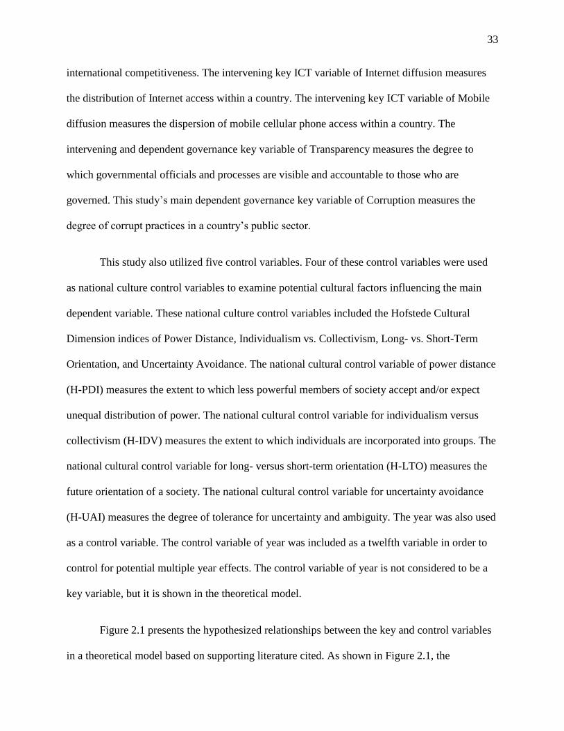
33
international competitiveness. The intervening key ICT variable of Internet diffusion measures
the distribution of Internet access within a country. The intervening key ICT variable of Mobile
diffusion measures the dispersion of mobile cellular phone access within a country. The
intervening and dependent governance key variable of Transparency measures the degree to
which governmental officials and processes are visible and accountable to those who are
governed. This study’s main dependent governance key variable of Corruption measures the
degree of corrupt practices in a country’s public sector.
This study also utilized five control variables. Four of these control variables were used
as national culture control variables to examine potential cultural factors influencing the main
dependent variable. These national culture control variables included the Hofstede Cultural
Dimension indices of Power Distance, Individualism vs. Collectivism, Long- vs. Short-Term
Orientation, and Uncertainty Avoidance. The national cultural control variable of power distance
(H-PDI) measures the extent to which less powerful members of society accept and/or expect
unequal distribution of power. The national cultural control variable for individualism versus
collectivism (H-IDV) measures the extent to which individuals are incorporated into groups. The
national cultural control variable for long- versus short-term orientation (H-LTO) measures the
future orientation of a society. The national cultural control variable for uncertainty avoidance
(H-UAI) measures the degree of tolerance for uncertainty and ambiguity. The year was also used
as a control variable. The control variable of year was included as a twelfth variable in order to
control for potential multiple year effects. The control variable of year is not considered to be a
key variable, but it is shown in the theoretical model.
Figure 2.1 presents the hypothesized relationships between the key and control variables
in a theoretical model based on supporting literature cited. As shown in Figure 2.1, the
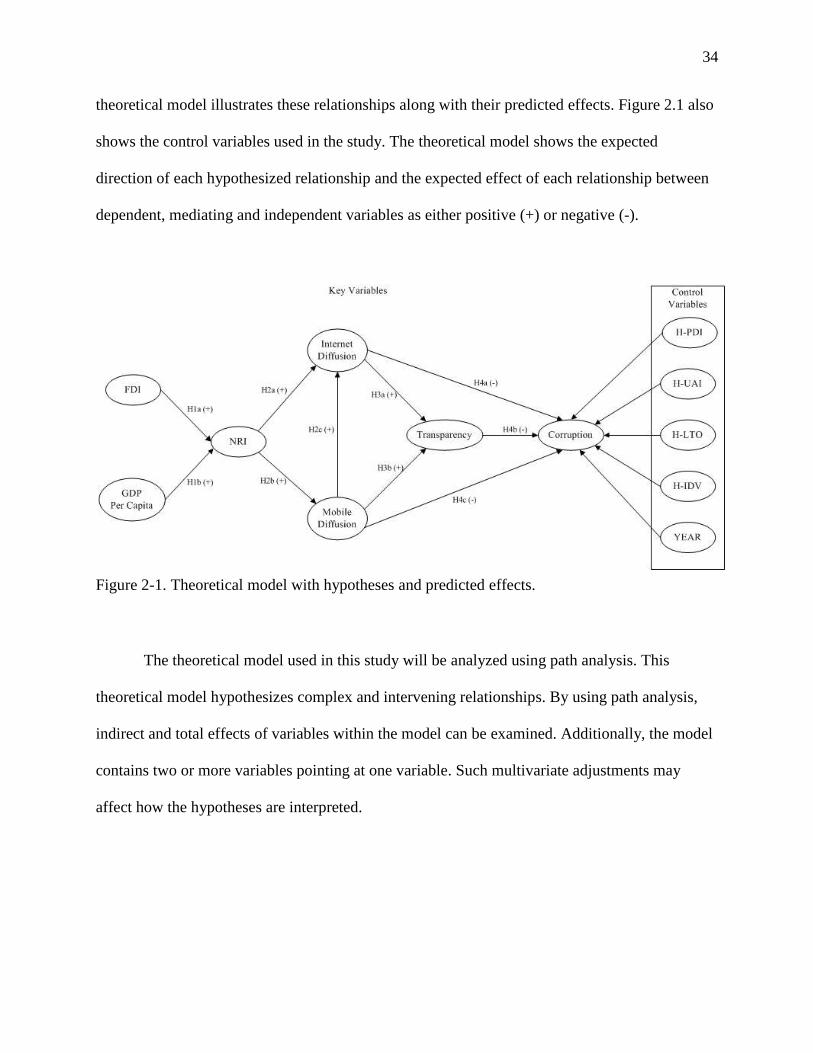
34
theoretical model illustrates these relationships along with their predicted effects. Figure 2.1 also
shows the control variables used in the study. The theoretical model shows the expected
direction of each hypothesized relationship and the expected effect of each relationship between
dependent, mediating and independent variables as either positive (+) or negative (-).
Figure 2-1. Theoretical model with hypotheses and predicted effects.
The theoretical model used in this study will be analyzed using path analysis. This
theoretical model hypothesizes complex and intervening relationships. By using path analysis,
indirect and total effects of variables within the model can be examined. Additionally, the model
contains two or more variables pointing at one variable. Such multivariate adjustments may
affect how the hypotheses are interpreted.

35
CHAPTER III
METHODOLOGY
The research design and methodology are explained in this section. In the first part of this
section, an overview of the sample countries used in the study is provided. In the second part of
this section, the variables used in the study are presented along with a focus on data collection
and data sources. In the third part of this section, a detailed description of each variable is
provided. In the fourth part of this section, the methods used to prepare the data for analysis such
as completeness and multicollinearity tests are described. Finally, in the fifth and final part of
this section, the method of data analysis is described.
3.1 Sample Design
As of 2012, there were 193 existing sovereign states and countries (United Nations,
2012). This study examined 121 countries of those 193 countries. Table 3-1 provides a list of the
countries selected for analysis in this study. Countries were selected for inclusion in the study
based on data availability of the key variables. The countries used in this study are representative
of a diverse range of economic and political structures. The key and control variables used in this
study are enumerated and described in section 3.3: Variable Description. This study used multi-
year data for these key and control variables collected over a period from 2006 to 2010.
The study excludes 72 sovereign states and countries. These sovereign states and
countries were excluded due to lack of data availability of the key variables (Messner, 1992).
Key variable data was collected from several multinational datasets from various sources such as
the World Bank World Development Indicators, World Economic Forum Global Information

36
Technology Report, World Bank Worldwide Governance Indicators, and Transparency
International.
Table 3-1. List of countries used in this study.
Albania Denmark Lesotho Romania
Algeria Dominican
Republic Lithuania Russia
Angola Ecuador Luxembourg Singapore
Argentina Egypt Macedonia Slovakia
Armenia El Salvador Madagascar Slovenia
Australia Estonia Malawi South Africa
Austria Ethiopia Malaysia South Korea
Azerbaijan Finland Mali Spain
Bahrain France Malta Sri Lanka
Bangladesh Georgia Mauritania Suriname
Barbados Germany Mauritius Sweden
Belgium Greece Mexico Switzerland
Benin Guatemala Moldova Taiwan
Bolivia Guyana Mongolia Tanzania
Bosnia-Herzegovina Honduras Morocco Thailand
Botswana Hong Kong Mozambique Trinidad and Tobago
Brazil Hungary Namibia Tunisia
Bulgaria Iceland Nepal Turkey
Burkina Faso India Netherlands Uganda
Burundi Indonesia New Zealand Ukraine
Cambodia Ireland Nicaragua United Arab Emirates
Cameroon Israel Nigeria United Kingdom
Canada Italy Norway USA
Chad Jamaica Pakistan Uruguay
Chile Japan Panama Venezuela
China Jordan Paraguay Vietnam
Colombia Kazakhstan Peru Zambia
Costa Rica Kenya Philippines Zimbabwe
Croatia Kuwait Poland
Cyprus Kyrgyzstan Portugal
Czech Republic Latvia Qatar

37
3.2 Data Collection
Data for the key and control variables was collected by country and year using several
online databases for the 121 countries used in this study. Table 3-2 summarizes the key and
control variables and their related data sources. Data for the macroeconomic variables of FDI
and GDP per capita used in this study were collected from the World Bank World Development
Indicators. Data for the ICT variables of Internet diffusion and Mobile diffusion used in this
study were collected from the World Bank World Development Indicators. Data for the ICT
variable of NRI used in this study was collected from the World Economic Forum Global
Information Technology Report.
Table 3-2. Data sources for variables.
Variable Measure Source
Transparency Voice and Accountability Indicator World Bank Worldwide
Governance Indicators
Corruption Corruption Perceptions Index Transparency International
Internet diffusion Internet users (per 100 people) The World Bank World
Development Indicators
Mobile diffusion Mobile cellular subscriptions per
100 people
The World Bank World
Development Indicators
FDI Foreign direct investment, net
inflows (balance of payments,
current US$)
The World Bank World
Development Indicators
NRI Networked Readiness Index World Economic Forum Global
Information Technology Report
GDP per capita Gross Domestic Product per capita
(current US$)
The World Bank World
Development Indicators
H-PDI Power Distance Index Hofstede Dimension Data Matrix
H-UAI Uncertainty Avoidance Index Hofstede Dimension Data Matrix
H-LTO Long-Term Orientation Index Hofstede Dimension Data Matrix
H-IDV Individuality Index Hofstede Dimension Data Matrix

38
Data for the variable of Transparency used in this study was collected from the World
Bank Worldwide Governance Indicators. Data for the variable of Corruption used in this study
was collected from Transparency International’s Corruption Perceptions Index. Data for the
national culture control variables of Power Distance Index, Uncertainty Avoidance Index, Long-
Term Orientation Index, and Individuality Index used in this study was collected from the
Hofstede Cultural Dimension scores gathered through the Geert Hofstede Dimension Data
Matrix as presented in Cultures and Organizations 3rd
edition (Hofstede et al., 2010). The total
dataset consisted of 605 rows. Table 3-3 presents the key and control variables with the number
of data items collected for each year.
Table 3-3. Number of data items collected for each variable by year.
Variable 2006 2007 2008 2009 2010 Total
Transparency 121 121 121 121 121 605
Corruption 120 120 121 121 120 602
Internet diffusion 119 119 119 119 120 596
Mobile diffusion 119 119 119 118 120 595
FDI 120 120 120 120 120 600
NRI 121 118 120 119 116 594
GDP per capita 120 120 120 120 120 600
H-PDI 75 75 75 75 75 375
H-UAI 75 75 75 75 75 375
H-LTO 86 86 86 86 86 430
H-IDV 75 75 75 75 75 375
3.3 Variable Description
This study explored the hypothesized relationships between macroeconomic, ICT,
governance and sociocultural variables using the key and control variables as listed in Table 3-3.
These relationships are put forth in the theoretical structural model as presented in Figure 2.1.

39
The independent and mediating variables in the theoretical model are Foreign Direct Investment,
Gross Domestic Product per capita, Networked Readiness Index, Internet diffusion, Mobile
diffusion, and Transparency. The intervening or mediating variables in the theoretical model are
Networked Readiness Index, Internet diffusion, Mobile diffusion, and Transparency. Finally, the
main dependent variable in the theoretical model is Corruption. The national culture control
variables used in this study were Hofstede’s Cultural Dimension indices of Power Distance,
Individuality, Long-Term Orientation, and Uncertainty Avoidance. A further enumeration and
detailed description of the key and control variables are presented below. Representations in the
data analysis and structural models of these key and control variables are presented in
parentheses.
The macroeconomic variable of Foreign Direct Investment (FDI) is the net inflow of
investment, measured in current U.S. dollars, into a domestic economy by foreign investors.
These investment inflows are shown in the balance of payments as financial transfers, including
the sum of equity capital, reinvestment of earnings, short-term and long-term capital. Data for
the variable of FDI was captured through foreign direct investment, net inflows (BoP, current
U.S. $) indicator from the World Bank World Development Indicators which is reported in
current U.S. dollars. The foreign direct investment, net inflows (BoP, current U.S.$) indicator as
contained in the World Bank World Development Indicators data were supplied by the
International Monetary Fund’s Balance of Payments database and supplemented by data from the
United Nations Conference on Trade and Development and other official national sources.
The FDI data values are quite large and varied -- ranging from hundreds of thousands to
hundreds of billions of U.S. dollars. The large and varied values of the FDI data tend to increase
variance. One method used in stabilizing variance is logarithmic data transformation (Bland,

40
2002). Logarithmic data transformation is the process of converting a data value into its
logarithmic value using some base such as the natural base (℮). Logarithmic transformations of
data can transform non-linear relationships into linear ones and normalize positively skewed
distributions (Sokal & Rohlf, 1969). Such logarithmic transformation allows easier handling and
interpretation of data values with a high degree of variance (Zar, 1999). A general logarithmic
transformation could not be performed because a few of the FDI data values were negative.
Therefore, the logarithmic transformation was performed on the absolute value of the FDI data
values. Depending on the sign of the original FDI data value, a logarithmic transformed value
was multiplied by a constant of +1 or -1 to represent its original sign. For example, negative FDI
data values, which represent divestiture or disinvestment, were represented by multiplying the
logarithmic transformation value by negative 1.
The macroeconomic variable of Gross Domestic Product per capita (GDP per capita)
measures the gross domestic product divided by the midyear population. Data for the variable of
GDP per capita data was captured through the gross domestic product per capita (current U.S. $)
indicator from the World Bank World Development Indicators and was measured in current U.S.
dollars. The gross domestic product per capita (current U.S.$) indicator data as contained in the
World Bank’s World Development Indicators was supplied by the World Bank national accounts
data and Organisation for Economic Co-operation and Development (OECD ) National Accounts
data files.
GDP per capita is the most widely used macroeconomic indicator of a country’s standard
of living (Ringen, 1991). There are some scholars who suggest that the GNP, instead of GDP, is
a more accurate measure of economy well-being and market activity (Brezina, 2012; Stiglitz,
2009). However, Bureau of Economic Analysis (1991) has stated that “virtually all other

41
countries have already adopted GDP as their primary measure of production” (p. 8). Studies
researching the relationships between macroeconomic and ICT variables generally use GDP or
GDP per capita to measure economic activity and growth (Addison & Heshmati, 2004; Dewan et
al., 2005; Kiiski & Pohjola, 2002).
The ICT variable of Networked Readiness Index (NRI) measures the degree to which a
country is positioned to use its ICT infrastructure for international competitiveness. Data for the
variable of NRI was captured through the Networked Readiness Index index score as published
in the Global Information Technology Report by the World Economic Forum together with
INSEAD (French name "INStitut Européen d'ADministration des Affaires", or European
Institute of Business Administration). The Networked Readiness Index as published in the Global
Information Technology Report is comprised of two parts: an index score and a rank. In this
study, only the index score was used as the measure of analysis. The index score is a composite
of three component indexes: environment, readiness, and usage. The environment component
index and its subcomponents examine the market, political, regulatory, and infrastructure
conditions that facilitate or hamper ICT growth. The readiness component index and its
subcomponents examine the readiness and preparedness of individuals, governments, and
businesses to utilize ICT resources. The usage component index and its subcomponents examine
the levels of usage among individuals, governments, and businesses. The composite index,
ranging from 1.0 (worst) to 7.0 (best), provides a method for a) calculating the relative and
overall development and use of ICT in countries and b) understanding the strengths and
weaknesses of a country’s ICT readiness to compete in a global environment. The rank is the
particular country’s numerical rank based on the index score.

42
This study utilized two variables to measure ICT diffusion. These two ICT variables
include Internet diffusion and Mobile diffusion. The ICT variable for diffusion of Internet
(Internet diffusion) measures the distribution of Internet access within a country. Data for the
variable of Internet diffusion data was captured through the Internet users (per 100 people)
indicator from the World Bank World Development Indicators. The Internet users (per 100
people) indicator measures the number of persons per 100 people of a country’s population who
have access to the Internet. Data for the Internet users (per 100 people) indicator as contained in
The World Bank World Development Indicators were supplied by the International
Telecommunication Union’s World Telecommunication/ICT Development Report and World
Bank estimates. The International Telecommunications Union (ITU) is a special agency of the
United Nations responsible for global information and communication technologies
coordination.
The ICT variable of mobile cellular diffusion (Mobile diffusion) measures the dispersion
of mobile cellular phone access within a country. Data for the variable of Mobile diffusion was
captured through the Mobile cellular subscriptions (per 100 people) indicator of the World Bank
World Development indicators. This indicator measures the number of persons per 100 people of
a country’s population who have subscriptions to public mobile telephone services using cellular
technology. These service subscriptions provide access to the public switched telephone
network. Prepaid and post-paid subscriptions were included in the indicator.
Data for the Mobile cellular subscriptions (per 100 people) indicator as contained in the
World Bank World Development Indicators were supplied by the International
Telecommunication Union’s World Telecommunication/ICT Development Report and database,
and World Bank estimates.

43
The governance variable of Transparency (Transparency) measures the degree to which
governmental officials and processes are visible and accountable to those who are governed.
Data for the variable of Transparency was captured through the Voice and Accountability (VA)
indicator of the World Bank’s Worldwide Governance Indicators. The Voice and Accountability
(VA) indicator forms one of six World Bank governance indicators. The Worldwide Governance
Indicators are a set of six indicators for 215 world economies. These six indicators are: Voice
and Accountability, Political Stability and Absence of Violence, Government Effectiveness,
Regulatory Quality, Rule of Law, and Control of Corruption.
The Voice and Accountability (VA) indicator measures the extent to which a country’s
citizens are able to participate in their governance by examining several aspects of a country’s
political processes, including civil liberties, political rights, and a free media (Kaufmann, Kraay,
& Mastruzzi, 2009). As presented in Table 3-4, the Voice and Accountability (VA) indicator is a
composite of twenty representative and non-representative data source types such as government
and public sector (GOV), non-governmental organizations (NGO), commercial business
information providers (CBIP), and surveys of households and firms (SURVEY). The Voice and
Accountability (VA) indicator, ranging from around ‐2.5 to 2.5, measures countries’
accountability and citizen participation in relation to the global average (equaling zero).
This composite indicator served as a measure for transparency in this study since public
voice and methods of accountability in a society create a perception of more transparency
(Andrea & Antonio, 2007). The variable of Transparency served as a dependent and intervening
variable in this study.

44
Table 3-4. Voice and Accountability (VA) indicator data types and sources.
Source Type*
African Electoral Index (IRP) NGO
Afro-barometer (AFR) GOV
Bertelsmann Transformation Index (BTI) NGO
Cingranelli Richards Human Rights Database and Political Terror Scale
(HUM)
GOV
Economist Intelligence Unit Risk-wire & Democracy Index (EIU) CBIP
Freedom House (FRH) NGO
Freedom House Countries at the Crossroads (CCR) NGO
Gallup World Poll (GWP) SURVEY
Global Insight Business Conditions and Risk Indicators (WMO) CBIP
Global Integrity Index (GII) NGO
IFAD Rural Sector Performance Assessments (IFD) GOV
Institute for Management and Development World Competitiveness Yearbook SURVEY
Institutional Profiles Database (IPD) GOV
International Budget Project Open Budget Index NGO
Latino-barometro SURVEY
International Research and Exchanges Board Media Sustainability Index NGO
Political Risk Services International Country Risk Guide (PRS) CBIP
Reporters Without Borders Press Freedom Index (RSF) NGO
Vanderbilt University Americas Barometer SURVEY
World Economic Forum Global Competitiveness Report (GCS) SURVEY
Note: “type” refers to the nature of the data source. Data sources for Voice and Accountability
are from government and public sector (GOV), non-governmental organizations (NGO),
commercial business information providers (CBIP), and surveys of households and firms
(SURVEY).
The governance variable for Corruption (Corruption), the main dependent variable in this
study, measures the degree of corrupt practices in a country’s public sector. The data for the
variable of Corruption was captured through the Corruption Perceptions Index (CPI) from
Transparency International. This index measures the degree of corruption that exists among
public officials and politicians (Lambsdorff, 1999a). The CPI is the most disseminated among
policymakers and is a composite index that includes survey data from country experts,
businesspeople, global analysts, and experts who are residents of the evaluated countries

45
(Svensson, 2005). The CPI focuses on perceptions of public sector corruption – the use of public
office for private gain.
The CPI index ranks countries on a scale from 10 (representing a very clean/minutely
corrupt government) to 0 (representing a highly corrupt government). On the CPI scale, countries
with lesser perceptions of corruption score higher. Thus, the CPI scale lends itself to be
interpreted as ‘the absence of corruption’ perception index. To make the CPI values reflect the
presence of corruption, a data transformation was performed on the CPI data. The original CPI
values were multiplied by the constant of negative 1 to inverse the scaling while preserving the
rank of the values. This data transformation resulted in highly corrupt countries having a higher
value than those with lower levels of perceived corruption.
Given the potential important influences of sociocultural values on corruption and ICT
diffusion, this study included four Hofstede’s Cultural Dimension indices as national culture
control variables. Husted (1999) found that corruption was significantly correlated to the
Hofstede cultural dimensions of power distance, masculinity, and uncertainty avoidance.
According to Myrdal (1970a), corruption is defined, in part, by sociocultural mores and values.
Furthermore, many scholars suggest that corruption can be defined in sociocultural terms
(Friedrich, 1989; Johnston, 1997; Rose-Ackerman, 1978, 1996). Also, several authors such as N.
Rosenberg (1972), Erumban and de Jong (2006), Moghadam and Assar (2008), Jakopin and
Klein (2011), suggest that sociocultural values influence individuals in a society in a way that
facilitates or impedes technology adaptation and diffusion. For example, Erumban and de Jong
(2006) found that countries with high power distance and uncertainty avoidance have lower ICT
adoption rates.

46
This study used the Hofstede’s Cultural Dimension indices of Power Distance (H-PDI),
Individuality (H-IDV), Long-Term Orientation (H-LTO), and Uncertainty Avoidance (H-UAI)
as national culture control variables to address potential influences of sociocultural factors. Data
for the national culture variables were imputed from the Hofstede Cultural Dimension scores for
each country used in the study. The Hofstede Cultural Dimension scores were gathered from the
Geert Hofstede Dimension Data Matrix as presented in Cultures and Organizations 3rd
edition
(Hofstede et al., 2010). The Hofstede Cultural Dimension indices are the resulting work of Geert
Hofstede research into cultural dimensions of a society and how these dimensions of culture
affect behavior. In 1967, Hofstede began a large scale survey study on differences in cultural
values of employees in different subsidiaries of IBM Europe. Hofstede compared answers of tens
of thousands of employees in over 40 countries. The analysis of the surveys identified four
anthropological systematic differences in national cultures: power distance, individualism,
uncertainty avoidance, and masculinity (Hofstede, 1984). In 1991, Hofstede added the additional
cultural dimension of long term orientation (Hofstede, 1997).
The Hofstede Cultural Dimension indices contained power distance, individualism,
uncertainty avoidance, masculinity and long term orientation scores for 110 countries and
regions. However, there were some countries that had missing scores within Hofstede-defined
regions. These missing scores were replaced with regional data scores. For example, Egypt did
not have scores for the four Hofstede cultural dimension indices. However, Egypt is classified
within a region of Arab countries which had regional Hofstede Cultural Dimension scores.
Therefore, Egypt’s missing country scores were replaced by the Arab regional scores. This
method of imputation of missing data using regional scores was the first method used to achieve
completeness of the Hofstede Cultural Dimension data. After this missing data method was

47
applied, the cultural dimension data was examined for completeness and further missing data
treatments were employed. These further missing data treatments are outlined and detailed in
section 3.4 Data Preparation. A description of each Hofstede Cultural Dimension index used in
this study follows. The year for the country observations was also used as a control variable.
The national cultural control variable for power distance (H-PDI) measures the extent to
which less powerful members of society accept and/or expect unequal distribution of power.
Societies which score higher in this Hofstede dimension value suggest that societal inequality is
more widely accepted by those who are governed. Data for the variable of power distance was
captured through Hofstede Cultural Dimension Power Distance index. The national cultural
control variable for individualism (H-IDV) measures the extent to which individuals are
incorporated into groups. Societies which score higher in this Hofstede dimension, value
personal rights and freedoms over collectivistic values (e.g. group loyalty). Data for the variable
of individualism was captured through Hofstede Cultural Dimension Individualism vs.
Collectivism Index. The national cultural control variable for long-term orientation (H-LTO)
measures the future orientation of a society. Societies which score higher in this Hofstede
dimension are seen as more future-oriented and foster more pragmatic views such as persistence.
Short-term orientation societies promote past and present values such as tradition, saving face,
etc. Data for the variable of long-term orientation was captured through Hofstede Cultural
Dimension Long- vs. Short-Term Orientation Index. The national cultural control variable for
uncertainty avoidance (H-UAI) measures the degree of tolerance for uncertainty and ambiguity.
Societies with higher scores in this Hofstede dimension generally have more rules and laws and
are less tolerant to unplanned change. Data for the variable of uncertainty avoidance was
captured through Hofstede Cultural Dimension Uncertainty Avoidance Index.

48
3.4 Data Preparation
A primary step before data analysis can be done is data preparation. One of the first steps
in data preparation is examining the dataset for completeness. This examination involves
reviewing the dataset for missing data and assessing the reason for such missing data. Missing
data can have a significant effect on research results. Missing data analysis is not generally the
main focus of scientific inquiry but must be addressed to prevent results that are “biased,
inefficient (lacking in power), and unreliable.” (Schafer & Graham, 2002, p. 147). A general rule
is to have no more than 10% of data missing in any column used in the data analysis; a more
relaxed rule for the missing data threshold is 20% (Allison, 2001; Hair, Anderson, & Tatham,
1987; Hair, Black, Babin, & Anderson, 2010).
This study combines data elements from several multinational datasets from various
sources such as the World Bank World Development Indicators, World Economic Forum Global
Information Technology Report, World Bank Worldwide Governance Indicators, and
Transparency International. As reported by Messner (1992), there tends to be missing data in
cross-national research because national government often does not report such critical statistics
consistently. Given the multinational datasets used in this study and the possibly of missing data,
an analysis for missing data was conducted on the dataset. As presented in Table 3-5, the
independent, mediating, and dependent variables were well within the 10% allowable missing
data threshold as suggested by Hair et al. (1987). However, several Hofstede Cultural Dimension
index variables exceeded both the 10% and 20% missing data thresholds. Given this amount of
missing data in the Hofstede Cultural Dimension index variables, a method of handling missing
data needed to be applied to the dataset.

49
Table 3-5. Percentage of missing data values by variable (N=605).
Variable Percentage of missing data
Transparency 0.000%
Corruption 0.496%
Internet diffusion 1.488%
Mobile diffusion 1.653%
FDI 0.826%
NRI 1.818%
GDP per capita 0.826%
H-PDI* 38.017%
H-UAI* 38.017%
H-LTO* 28.926%
H-IDV* 38.017%
Note: ‘*’ denotes variables with missing data values over the 10% and 20% missing data
thresholds as suggested by Hair et al. (1987)
There are several ways to address missing data in the statistics literature (Allison, 2001,
2003; Enders & Bandalos, 2001; Honaker & King, 2010; Little, 1988; Little & Rubin, 1987;
Olinsky, Chen, & Harlow, 2003; Roth, 1994; Schafer & Graham, 2002). The phenomenon of
missing data values is known as the missingness of the data (Hawthorne & Elliott, 2005;
Lauritzen, 1995; Little, 1988). First, the reason for the missing data must be determined in order
to select the appropriate missing data treatment. There are three categorical reasons for missing
data: missing completely at random (MCAR), missing at random (MAR), or missing not at
random (MNAR) (J.-O. Kim & Curry, 1977; Little, 1988; Little & Rubin, 1987).
The first possible categorical reason for missing data is MCAR. Missing data is
considered MCAR if the data values missing are independent of the other variables of interest or
some unobserved variable. MCAR is also known as uniform non-response since values are
missing independently of any other variable in the study (Wang & Fitzmaurice, 2006). As the
names suggests, MCAR data is completely missing due to random chance. Stated another way, in

50
MCAR, any data value has approximately the same probability of being observed or unobserved
as any other data value. For example, a researcher distributes and collects 200 paper surveys and
10% of those surveys are returned completely blank. If the blank surveys were randomly not
completed, the missing data from those blank surveys could be considered MCAR. Data that is
MCAR reduces statistical power but does not produce bias since the missing data is not related to
other variables.
The next possible categorical reason for missing data is MAR, which is an alternative to
MCAR. In MAR, missing data-values are not dependent on the missing data item itself (Heitjan
& Basu, 1996). A special case of MAR is known as uniform non-response within class (Robins,
1997). In the special case of MAR uniform non-response within class, data values are missing
based on a particular class or group within the dataset. According to Heitjan and Basu (1996),
MCAR and MAR are “ignorability conditions” (p. 1) that allow particular interpretations to be
safely made without complex missing data models. For example, in MAR, unobserved data
values can be intuitively based on observed data values of similar data rows (Schafer & Graham,
2002). Using the aforementioned example, a researcher distributes and collects 200 paper
surveys and 10% of those surveys are returned partially blank (e.g. some questions were
skipped). If the unanswered questions in the surveys were randomly not completed, this missing
data could be considered MAR.
The last possible categorical reason for missing data is known as MNAR. For MNAR, the
conditions of MCAR and MAR do not hold. In MNAR, data-values are missing not at random.
In the case of MNAR, data is missing based on the nature or value of the missing figures. Data
that is MNAR requires more complex missing data treatments and modeling. Also, determining
and compensating for the underlying reasons for the missingness proves to be more problematic.

51
The best way to obtain estimates of the missing data without introducing additional bias is to
create a model to mimic the missingness in the data (Dunning & Freedman, 2007). Using the
aforementioned example, a researcher distributes and collects 200 paper surveys and 10% of
those surveys are returned partially blank (e.g. some questions were skipped). The researcher
reviews the surveys and discovers that a particular group (e.g. women under thirty) skipped a
particular question (e.g. income). This commonality existing between the group and the
unanswered question signifies that the data is MNAR.
As shown in Figure 3.5, the Hofstede Cultural Dimension data was missing for 28% to
38% of the counties in this study. The independent, mediating, and dependent variables in this
study did not need a missing data treatment applied as these variables were within the 10%
allowable missing data threshold as suggested by Hair et al. (1987). To determine the best
method of handling the missing Hofstede Cultural Dimension data, the reason for why the data
was missing must be categorized into one of the three causes as suggested by Little and Rubin
(1987). In other words, were the missing cultural dimension values for countries in Hofstede’s
study related to the actual values of those cultural dimensions, or were they associated with some
other variable of interest?
According to Hofstede (1984), the cultural dimensions data that was missing for several
countries was a result of no IBM subsidiaries existing in those countries at the time of the
original data collection. The missing Hofstede Cultural Dimension data could be MNAR if IBM
selected countries in which to place subsidiaries based on some cultural dimension variable or
other unobserved variable. It is quite plausible for a global country such as IBM to exercise
diligence in placing its subsidiaries. While the explanation of selection bias by IBM is plausible,
at the time of Hofstede’s data collection, IBM had subsidiaries in more than seventy countries

52
(Hofstede, 1984). For the purpose of this study, it must be determined if there is a selection bias
in the Hofstede cultural dimensions data. To determine if IBM selected countries in which to
place subsidiaries based on some cultural dimension, the observed Hofstede cultural dimension
data was analyzed for non-normal distribution.
A test for non-normal or asymmetrical distribution is essentially a skewness test using the
adjusted Fisher-Pearson standardized moment coefficient (Doane & Seward, 2011). The test for
skewness exposes whether observed data values are asymmetrically distributed around the mean.
The test for skewness produces a skewness statistic that can be used to determine the degree of
asymmetry in the distribution of data. A distribution of data that is relatively symmetrical
produces a skewness statistic of near zero. A negative skewness statistic indicates more values
lay above the mean. A positive skewness statistic indicates more data values lay below the mean.
If IBM selected countries in which to place subsidiaries based on some cultural dimension, there
is a high probability that such a selection bias would skew the observed data values toward the
IBM-preferred bias.
Doane and Seward (2011) suggest using the adjusted Fisher-Pearson standardized
moment coefficient to test for skewness. The adjusted Fisher-Pearson standardized moment
coefficient includes an adjustment for sample size and is readily available in software packages
such as Minitab, Excel, SPSS, SAS and (Doane & Seward, 2011). The skewness statistic (S)
produced by the adjusted Fisher-Pearson standardized moment coefficient must be compared to a
threshold of allowable skewness. Tabachnick and Fidell (1996) suggest calculating the “standard
error of skewness – Ss” (p. 79) by using √ where N is the numbers of observed data
values. The probability of a large degree of skewness can be evaluated by using the z distribution

53
of as suggested in Tabachnick and Fidell (1996). A z value in excess of ±2.58
would indicate a significant degree of skewness in the distribution of data.
Presented in Table 3-6 are the results of the normal distribution test on the Hofstede
cultural dimension data. These results were calculated using Microsoft Excel 2010. Other
variables in this study were not tested for normal distribution as these variables were within the
10% allowable missing data threshold as suggested by Hair et al. (1987). Hofstede Cultural
Dimension data was tested for symmetric distribution to determine if IBM used some selection
bias in choosing countries in which to place subsidiaries. If IBM had exercised some bias in the
selection of countries, the observed data values would display this bias through an asymmetric
distribution of the Hofstede Cultural Dimension index data values
As presented in the results shown in Table 3-6, the Hofstede Cultural Dimension index
variables of power distance index (H-PDI) and long term orientation (H-LTO) did not present a
significant degree of asymmetric distribution based on the z-distribution threshold of z = ±2.58.
The Hofstede Cultural Dimension index variables of uncertainty avoidance (H-UAI) and
individualism (H-IDV), did present asymmetric distribution over the threshold of z = ±2.58 as
suggested by Tabachnick and Fidell (1996).
Table 3-6. Results of normal distribution test on Hofstede data.
Variable Mean Median St. Dev. S Ss z
H-PDI 59.680 64 21.077 -0.151 0.126 -1.197
H-UAI 66.307 68 22.815 -0.361 0.126 -2.857
H-LTO 46.592 45.466 22.951 0.294 0.118 -2.485
H-IDV 42.933 38 23.4112 0.346 0.126 2.739
Note: The skewness statistic (S) was produced by the adjusted Fisher-Pearson standardized
moment coefficient. The standard error of skewness Ss and z distribution calculations were
produced as suggested in Tabachnick and Fidell (1996).
54
The findings as presented in Table 3-6 suggest that IBM subsidiaries had a tendency to be
located in countries with higher values of uncertainty avoidance and lower values of
individuality. The asymmetric distribution found in the two Hofstede Cultural Dimensions
suggests that the Hofstede missing data values may not be MCAR. However, these findings do
not necessarily demonstrate that the Hofstede Cultural Dimension missing data is MNAR. The
Hofstede Cultural Dimensions index variables of power distance (H-PDI) and long term
orientation (H-LTO) did not present a significant degree of asymmetric distribution.
One explanation for some of the Hofstede Cultural Dimensions indices possessing an
asymmetric distribution is that some cultural dimensions are naturally asymmetrically
distributed. If some cultural dimensions are naturally asymmetrically distributed, then the
missing cultural dimension data values were unrelated to the unobserved value. This explanation
makes the assumption that the missing Hofstede Cultural Dimensions are MAR within a class of
countries. Specifically, the missing Hofstede Cultural Dimension data is unobserved for the class
of countries that did not have IBM subsidiaries. As stated by Robins (1997), MAR within class
data values are missing based on a particular group within the dataset.
The assumption of MAR for the missing Hofstede Cultural Dimensions data allows
particular interpretations to be safely made without utilizing complex missing data models
(Heitjan & Basu, 1996). A more complex missing data treatment would be required if the
Hofstede Cultural Dimensions data were MNAR. Collins, Schafer, and Kam (2001) have
demonstrated that under most missing data cases, even an erroneous assumption of MAR has
“only a minor impact on estimates and standard errors” (p. 6). It is important to note that
unobserved MAR data values can be intuitively based on observed data values of similar data
rows (Schafer & Graham, 2002).

55
This study used two missing data treatments: removal of non-complete data rows through
listwise deletion and data imputation through a modified version of mean substitution. The most
common and least complex treatment of missing data is listwise deletion. Listwise deletion is
also known as complete-case analysis (Schafer & Graham, 2002). This treatment requires the
deletion of non-complete cases (i.e. data rows missing one or more data values) until the level of
missing data is within an acceptable threshold. Statistical power may be affected by using
listwise deletion as a missing data treatment due to the reduction of the sample size and
introduction of bias if the data is not MAR or MCAR (King, Honaker, Joseph, & Scheve, 1998;
Roth, 1994). While this treatment affects statistical power and may introduce bias, it is one of the
preferable methods for addressing missing data (Olinsky et al., 2003).
The listwise deletion missing data treatment was applied to the data used in the study by
removing all data rows which did not contain values for all four Hofstede Cultural Dimension
index variables. This application resulted in the deletion of 145 data rows or 23.967% from the
original 606 data rows in the dataset. The data treated using listwise deletion treatment was
denoted as LD in this study. Presented in Table 3-7 are the resulting missing data percentages by
variable after the application of the listwise deletion treatment. As presented in Table 3-7, after
the listwise deletion treatment, all variables were within the relaxed 20% missing data threshold
(Allison, 2001; Hair et al., 1987; Hair et al., 2010).
The two basic methods of handling missing data are removal of incomplete cases or
imputation of missing data elements within incomplete cases (Little & Rubin, 2002). Although
removal of non-complete cases through listwise deletion is the most common and least complex
treatment for missing data, J.-O. Kim and Curry (1977), Roth (1994), and King et al. (1998)
suggest that alternate methods for handling missing data should be explored.

56
Table 3-7. Missing data percentages after listwise deletion (N=461).
Variable Missing data percentage
Transparency 0.000%
Corruption 0.652%
Internet diffusion 1.087%
Mobile diffusion 1.304%
FDI 1.087%
NRI 1.087%
GDP per capita 1.087%
H-PDI 18.478%
H-UAI 18.478%
H-LTO 6.522%
H-IDV 18.478%
The alternative to removing missing data from the dataset is to substitute missing values
to form a complete case or data row. This process of missing data substitution is known as
imputation (Schafer & Graham, 2002). As noted by Little and Rubin (2002), there are several
methods of imputation. Some methods of imputation such as hot/cold-deck imputation employ
random data value substitution (Sande, 1983) or intuitively-based substitution using observed
data values of similar data rows (Schafer & Graham, 2002). Such substitution methods select
existing data values from within the existing dataset to replace missing data values. Random data
value substitution is a straightforward and less complex method for handling missing data
(Reilly, 1993). In this study, however, such random substitution has a high probability of
assigning Hofstede Cultural Dimensions values that may be vastly different than the actual
unobserved values for a given country. A different imputation method needed to be explored that
would estimate data values similar to those actual unobserved values.
Another method for handling missing data is through imputation via mean substitution
(Dodeen, 2003). Typically, mean substitution is performed by calculating the mean for an entire

57
set of values of a variable. This calculated mean is substituted for the missing values of that
variable in the dataset. Using mean substitution creates a “group average” that is substituted for
the missing data values. In most cases, mean substitution has proven to be more accurate than
listwise deletion (Chan & Dunn, 1972; Chan, Gilman, & Dunn, 1976; Raymond & Roberts,
1987). In this study, mean substitution essentially creates world averages for each Hofstede
Cultural Dimension index. These world averages would then be applied to all countries with
unobserved Hofstede Cultural Dimension index values. As Hofstede Cultural Dimension values
are missing for 28% to 38% of the countries used in this study, these calculated world averages
would be applied to a significant number of countries. It is unreasonable to assume that up to
38% of the countries would have the same Hofstede Cultural Dimension values and those values
would be the same as the world averages. Therefore, the mean substitution method has high
probability of assigning world-average Hofstede Cultural Dimension values that may be vastly
different than the actual unobserved values for a particular country.
Fortunately, a further examination of the Hofstede Cultural Dimension studies provides
an indication on how data imputation through a modified version of mean substitution could
adequately handle the missing cultural dimension data values. Hofstede’s studies demonstrated
that cultural similarities that influenced behavior of societies could be categorized by nations and
regions (Hofstede, 1984, 1997). Some countries in the Hofstede Cultural Dimension score matrix
do not have scores for all four of Hofstede cultural dimensions used in this study. However, in
the Hofstede Cultural Dimension index, cultural dimension data values are provided for regional
country groups as well. In these regional groups, each component country can be assigned the
regional score as its individual country’s Hofstede Cultural Dimension index value. For example,
Nigeria did not have scores for all four Hofstede Cultural Dimension indices. However, Nigeria

58
is classified in the regional group of West African countries. The regional group of West African
countries includes Ghana, Nigeria, and Sierra Leone. Therefore, the scores for the regional group
of West African countries could be used in place of the missing Hofstede Cultural Dimension
data values for these three countries.
This study employed a modified version of mean substitution using the calculated mean
cultural dimension scores of regional groups to address missing Hofstede Cultural Dimension
index values. Countries used in this study were assigned to regional groups according to the
United Nations (UN) geoscheme. This geoscheme was developed by the UN for statistical
analysis of world regions (United Nations, 2000). Each UN geoscheme region has an associated
area code as its identifier within the UN statistical analysis model. For the countries used in this
study, there were sixteen UN geoscheme regions as presented in Table 3-8.
Table 3-8. United Nations geoscheme regions (with area codes).
Caribbean (052) Middle Africa (017) Southern Asia (034)
Central America (013) Northern Africa (012) Southern Europe (039)
Central Asia (143) Northern Europe (154) Western Africa (011)
Eastern Africa (014) South America (068) Western Asia (145)
Eastern Asia (030) South-Eastern Asia (035)
Eastern Europe (151) Southern Africa (018)
A mean score for each Hofstede Cultural Dimension was computed using available
cultural dimension scores of regional component countries based on the UN geoscheme. A mean
score for each UN geoscheme region was imputed for regional component countries missing data
values. For example, Algeria is in the UN geoscheme for Northern Africa. Algeria did not have
three of the four Hofstede cultural dimension scores used in this study. However, the Northern

59
Africa UN geoscheme region contained two other countries, Egypt and Morocco, which had
cultural dimension scores for the four Hofstede cultural dimensions. These available scores were
averaged per dimension and imputed for the missing three cultural dimension scores of Algeria.
This method of imputation using calculated regional mean scores of UN geoscheme
regions produced scores for all but two UN geoscheme regions used in this study. Central Asia
and Middle Africa were the only two UN geoscheme regions that did not have country-level
Hofstede Cultural Dimension scores from which to compute regional cultural dimension scores
through this method. The data using this modified mean substitution method was denoted as
regional mean substitution (RMS) in this study. This RMS imputation method was preferable
and advantageous over listwise deletion as it reduced missing data without reducing the overall
sample size. The missing data percentages by variable after using RMS missing data treatment
are presented in Table 3-9. As shown, all variables were well within a 10% missing data
threshold as suggested by Hair et al. (1987).
Table 3-9. Missing data percentages after regional mean substitution (N=605).
Variable Missing data percentage
Transparency 0.000%
Corruption 0.496%
Internet diffusion 1.488%
Mobile diffusion 1.653%
FDI 0.826%
NRI 1.818%
GDP per capita 0.826%
H-PDI 4.132%
H-UAI 4.132%
H-LTO 3.306%
H-IDV 4.132%

60
3.5 Data Validation
An analysis for multicollinearity was also performed on the data. Multicollinearity exists
when correlations among two or more independent or explanatory variables are strong. When
two or more variables are highly correlated, it may be an indication that variables which are
supposed to measure different constructs actually measure the same construct (Kline, 2010).
Multicollinearity exposes variables that may measure the same construct in a statistical model
(i.e. redundant variables). While multicollinearity may not affect the reliability of a statistical
model, it may not give accurate results on the significance of the effects of individual variables
within such a model (Kock, 2012).
One possible indicator of multicollinearity is a high Pearson correlation coefficient (r)
between two or more variables (Tabachnick & Fidell, 1996). High correlation coefficients among
variables in the model may signify multicollinearity (Kock, 2012). Correlation coefficients (r)
can range be from -1 to + 1. The closer the correlation coefficient is to ±1, the stronger the
correlation. A correlation coefficient of zero suggests there is no relationship. A general “rule of
thumb” (Farrar & Glauber, 1967, p. 82) for correlation coefficients that may indicate
multicollinearity are those where r ≥ .8. Using WarpPLS 3.0, a structural equation modeling
software package discussed in greater detail in section 3.5 Data Analysis, a correlation matrix
was generated with the data using both missing data treatments. WarpPLS 3.0 automatically
calculated the correlation matrix as part of its data analysis (Kock, 2012).
Table 3-10 shows the correlation matrix with corresponding coefficients and associated
p-values for data using regional mean substitution missing data treatment. Using the regional
mean substitution missing data treatment, NRI and corruption had a correlation coefficient of r =

61
-0.888 with a significance level of p <.001. NRI and Internet diffusion had a correlation
coefficient of r = 0.849 with a significance level of p <.001. GDP per capita and Internet
diffusion had a correlation coefficient of r = 0.828 with a significance level of p <.001. Also,
GDP per capita and NRI had a correlation coefficient of r = 0.829 with a significance level of p
<.001. Table 3-11 shows the correlation matrix with corresponding coefficients and associated p-
values for data using the listwise deletion missing data treatment. Using the listwise deletion
missing data treatment, NRI and corruption had a correlation coefficient of r = -0.907 with a
significance level of p <.001. NRI and Internet diffusion had a correlation coefficient of r =
0.857 with a significance level of p <.001. Analysis of the correlation matrixes using both
missing data treatments showed correlation coefficients among variables greater than r = 0.800.
The presence of a high correlation coefficient between two or more variables is a possible
indicator of multicollinearity. However, such high correlation coefficients do not conclusively
signify multicollinearity. High correlation coefficients are generally conflated with collinearity
(Douglass, Clader, Christy, Michaels, & Belsley, 2003 & Michaels, 2003; Graham, 2003). Yet,
strongly correlated variables can have a low degree of collinearity (Hamilton, 1987). Also, using
correlation matrices to assess multicollinearity only exposes potential bivariate collinearity.
Correlation matrices only compare variables in a pairwise fashion. Often, two or more variables
in a model may have collinear relationships which are not easily detected through such pairwise
analysis possible from correlation matrices (Tabachnick & Fidell, 1996). While analysis of
correlations provides a valuable indicator of multicollinearity, additional tests for
multicollinearity need to be performed.
Another method for assessing multicollinearity is the calculation of variance inflation
factors (VIFs). Unlike testing for collinearity through generating correlation matrices, the

62
calculation of VIF value assesses the amount of multicollinearity among all variables in a model
simultaneously. VIF values quantify the amount of inflation of variance due to a particular
variable in the model. The VIF value for a given variable is the amount of inflation of variance
caused by collinearity with other variables in the model (Kline, 2010; Kutner, Nachtsheim, &
Neter, 2004).
High VIF values may signify a high degree of multicollinearity. The threshold for high
VIFs is based on the type of variables used in a model. For example, the recommended VIF
threshold when using formative latent variables is VIF=3.3 (Cenfetelli & Bassellier, 2009). This
study does not use formative latent variable measurement, so this more restrictive threshold does
not need to be applied. For studies without latent variables, such as this study, a more relaxed
threshold recommendation of VIF=5 or VIF=10 has also been proposed in the multivariate
analysis literature (Hair et al., 1987; Hair et al., 2010; Kline, 2010; O'Brien, 2007).
There are two forms of collinearity which can be tested through calculating VIF values:
lateral and vertical collinearity. Lateral collinearity refers to predictor-criterion collinearity.
Lateral collinearity occurs when independent variables (i.e. predictor variables) are collinear
with the dependent variable (i.e. criterion variables) (Kock & Lynn, 2012). Vertical collinearity
refers to predictor-predictor collinearity.
Vertical collinearity occurs when independent variables (i.e. predictor variables) are
collinear with other independent variables. Using WarpPLS 3.0 to calculate VIF values through a
full collinearity test assesses vertical and lateral collinearity simultaneously (Kock, 2012). Also,
full collinearity VIF testing is a common method for testing bias that provides more conservative
results than exploratory factor analyses (Kock & Lynn, 2012; Lindell & Whitney, 2001).

63
Table 3-10. Correlation matrix for RMS treated data.
Transparency Corruption
Internet
diffusion
Mobile
diffusion FDI NRI
GDP per
capita H-PDI H-UAI H-LTO H-IDV
Transparency 1
Corruption -0.757***
1
Internet
diffusion 0.682
*** -0.793
*** 1
Mobile
diffusion 0.495
*** -0.570
*** 0.766
*** 1
FDI 0.301***
-0.432***
0.471***
0.387***
1
NRI 0.671***
-0.888***
0.849***
0.651***
0.555***
1
GDP per
capita
0.686***
-0.788***
0.828***
0.722***
0.505***
0.829***
1
H-PDI -0.614***
0.644***
-0.507***
-0.312***
-0.157***
-0.536***
-0.501***
1
H-UAI 0.022 0.160***
0.065 0.187***
0.002 -0.125**
0.082* 0.226
*** 1
H-LTO 0.212***
-0.234***
0.366***
0.289***
0.259***
0.354***
0.302***
-0.094* 0.092
* 1
H-IDV 0.547***
-0.601***
0.551***
0.380***
0.314***
0.531***
0.536***
-0.63***
-0.123**
0.303***
1
Year -0.013 0.003 0.185***
0.299***
-0.059 0.035 -0.003 0 0 0 0
Notes: Correlations between variables higher than 0.800 are denoted in bold.
*** denotes p-value <0.001
** denotes p-value <0.01
* denotes p-value <0.05
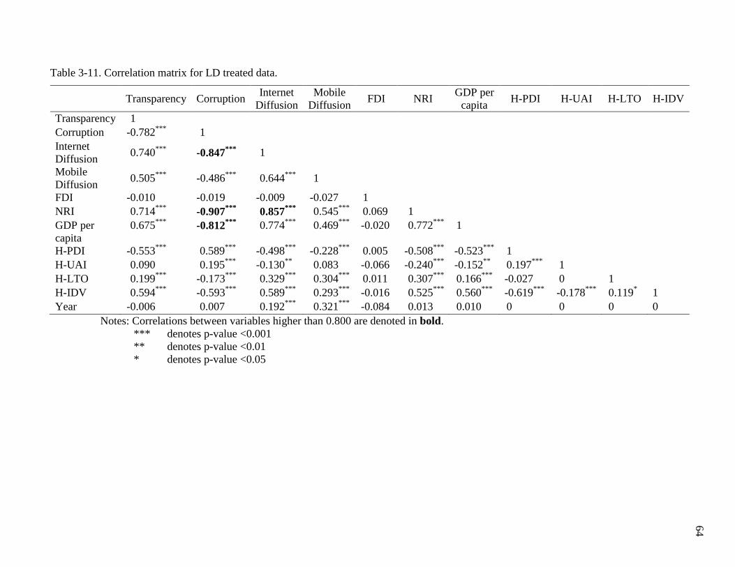
64
Table 3-11. Correlation matrix for LD treated data.
Transparency Corruption
Internet
Diffusion
Mobile
Diffusion FDI NRI
GDP per
capita H-PDI H-UAI H-LTO H-IDV
Transparency 1
Corruption -0.782***
1
Internet
Diffusion 0.740
*** -0.847
*** 1
Mobile
Diffusion 0.505
*** -0.486
*** 0.644
*** 1
FDI -0.010 -0.019 -0.009 -0.027 1
NRI 0.714***
-0.907***
0.857***
0.545***
0.069 1
GDP per
capita
0.675***
-0.812***
0.774***
0.469***
-0.020 0.772***
1
H-PDI -0.553***
0.589***
-0.498***
-0.228***
0.005 -0.508***
-0.523***
1
H-UAI 0.090 0.195***
-0.130**
0.083 -0.066 -0.240***
-0.152**
0.197***
1
H-LTO 0.199***
-0.173***
0.329***
0.304***
0.011 0.307***
0.166***
-0.027 0 1
H-IDV 0.594***
-0.593***
0.589***
0.293***
-0.016 0.525***
0.560***
-0.619***
-0.178***
0.119* 1
Year -0.006 0.007 0.192***
0.321***
-0.084 0.013 0.010 0 0 0 0
Notes: Correlations between variables higher than 0.800 are denoted in bold.
*** denotes p-value <0.001
** denotes p-value <0.01
* denotes p-value <0.05

65
65
A full collinearity test was performed that calculated the VIF values of each variable. The
full collinearity test was performed on the data using each missing data treatment. WarpPLS 3.0
automatically calculated the VIF values for the data as part of its data analysis (Kock, 2012).
Table 3-12 presents the VIF values for each variable in the data using both missing data
treatments.
The highest VIF value was 9.478 for corruption in the data using the listwise deletion
missing data treatment. In general, the data using the listwise deletion missing data treatment had
higher VIF values than the data using the regional mean substitution missing data treatment.
Data using each missing data treatment had VIF values over the recommended threshold of
VIF=5. However, using the more relaxed threshold of a VIF=10 as suggested by Hair et al.
(1987) and O'Brien (2007), the VIF values for the data using both missing data treatments did
not exhibit serious bias due to multicollinearity problems. Also, the variables that contribute to
the high VIF values in Table 3-12 are not included in the same variable block in Table 3-13 or
Table 3-14.
Table 3-12. Variance inflation factors by variable and missing data treatment.
Variable Data using RMS Data using LD
Transparency 2.784 3.672
Corruption 8.741 9.478
Internet diffusion 6.325 6.749
Mobile diffusion 2.523 2.059
FDI 1.045 1.036
NRI 8.004 8.089
GDP per capita 3.081 3.303
H-PDI 2.120 1.954
H-UAI 1.349 1.415
H-LTO 1.336 1.310
H-IDV 2.148 2.126
Year 1.286 1.337

66
66
Additionally, block VIF values for each missing data treatment were calculated by
WarpPLS 3.0. Block VIF values measure the degree of vertical collinearity. WarpPLS 3.0
outputs the VIF values for each latent variable block. A latent variable block is each variable
with two or more predictors. The calculated VIFs produced by WarpPLS 3.0 represent the latent
variables on each column (predictors), with reference to the latent variables on each row
(criteria). This study does not utilize latent variables, so the output from WarpPLS 3.0 comprises
the VIF values produced for each variable block.
Table 3-13 presents the block VIF values for the data using the RMS missing data
treatment for each variable block. Using the RMS missing data treatment, Transparency
(predictor) to Corruption (criteria) showed a VIF value of 4.588. Also, Internet diffusion
(predictor) to Corruption (criteria) showed a VIF value of 4.566.
All other VIF values for the data using the RMS missing data treatment were less than
3.3. Table 3-14 presents the block VIF values for the data using the LD missing data treatment
for each variable block. Using the LD missing data treatment, Transparency (predictor) to
Corruption (criteria) showed a VIF value of 4.769. Also, Internet diffusion (predictor) to
Corruption (criteria) showed a VIF value of 4.320. All other VIF values for the data using the
RMS missing data treatment were VIF less than 3.3. In the block VIF calculations, values of 3.3
or lower suggest that no vertical multicollinearity exists within the data (Kock, 2012). However,
in the multivariate analysis literature, a conservative recommended threshold for VIF values
when analyzing models without latent variables is VIF=5 as suggested by Hair et al. (1987).
Using this recommended threshold of VIF=5, the VIF values for the data using both missing data
treatments suggest that no vertical multicollinearity exist.

67
Table 3-13. Block VIF values using RMS.
Transparency Corruption
Internet
Diffusion
Mobile
Diffusion FDI NRI
GDP per
capita H-PDI H-UAI H-LTO H-IDV Year
Transparency 1.858 1.858
Corruption 4.588 4.566 1.831 2.804 1.084 1.250 2.512 1.096
Internet
Diffusion
1.886
1.886
Mobile
Diffusion
FDI
NRI 1.407 1.407
GDP per
capita
H-PDI
H-UAI
H-LTO
H-IDV
Year
Notes: These VIFs are for the latent variables on each column (predictors), with reference to the latent variables on each row (criteria).

68
Table 3-14. Block VIF using LD.
Transparency Corruption
Internet
Diffusion
Mobile
Diffusion FDI NRI
GDP per
capita H-PDI H-UAI H-LTO H-IDV Year
Transparency 1.652 1.652
Corruption 4.769 4.320 1.606 2.009 1.104 1.143 2.228 1.154
Internet
Diffusion
1.486
1.486
Mobile
Diffusion
FDI
NRI 1.366 1.366
GDP per
capita
H-PDI
H-UAI
H-LTO
H-IDV
Year
Notes: These VIFs are for the latent variables on each column (predictors), with reference to the latent variables on each row (criteria).

69
Additionally, Stone-Geisser Q-squared coefficients were calculated for each of the
endogenous variables in the study’s path model (Geisser, 1974; Stone, 1974). The resulting Q-
squared coefficients are shown for each missing data treatment in Table 3-15. The Q-squared
coefficient is used to assess the predictive validity of each variable block in a path model.
Endogenous variables with acceptable predictive validity have Q-squared coefficients of greater
than zero (Kock, 2012). Each of the endogenous variables in the study’s model exhibited Q-
squared coefficients greater than zero, thereby presenting acceptable predictive validity.
Table 3-15. Stone-Geisser Q-squared coefficients.
Transparency Corruption Internet Diffusion Mobile Diffusion NRI
RMS 0.486 0.795 0.789 0.475 0.738
LD 0.557 0.815 0.779 0.376 0.738
3.6 Data Analysis
The theoretical model for this study as shown in Figure 2.1 was constructed based on the
hypotheses as stated in Section 2.3. This theoretical model is a path model that formalized the
hypothesized relationships among the macroeconomic, ICT, governance, and sociocultural
variables as listed in Table 3-3. This theoretical model was statistically analyzed using path
analysis with WarpPLS 3.0, a structural equation modeling software package. WarpPLS 3.0 is
specially designed to identify nonlinear relationships among variables of a theorized model by
conducting linear and non-linear (or “warped”) regression analysis (Kock, 2012).
Path analysis is a statistical analysis method used to explore relationships among
observed variables within a defined network or model (Hatcher, 1994). Developed in the 1930s

70
by Sewall Wright, path analysis was used in his agricultural research and has now been applied
to other complex modeling fields (Dodge & Marriott, 2003; Wright, 1934). Path analysis is an
extension of multiple regression analysis. In multiple regression analysis, coefficients of
association are calculated among multiple independent variables and one dependent variable.
These coefficients are generally in the form of standardized partial regression coefficients
(Rencher, 1998; Rosenthal & Rosnow, 1991) where the corresponding P values indicate the
significance of the relationship (Kock, 2011a). Indeed, path analysis extends multiple regression
analysis by forming a composite structural model of several separate multiple regression models.
Path analysis allows the tracing of complex paths in a model to discover how one variable affects
another. This capability of path analysis allows direct and indirect effects to be explored. Also,
path analysis can reveal the proportional strengths of direct and indirect relationships within a
model.
Path analysis is a special case of structural equation modeling (SEM) (Maruyama, 1998).
SEM is a second-generation statistical analysis technique increasing utilization in social science
research due to its ability to assess theoretical models (Anderson & Gerbing, 1988; Kline, 2010).
Due to its powerful predictive ability, SEM has been used in a wide variety of disciplines,
including management (Cheng, 2001; Shook, Ketchen, Hult, & Kacmar, 2004), marketing
(Baumgartner & Homburg, 1996; Steenkamp & Baumgartner, 2000), information systems
(Gefen, 2000; Qureshi & Compeau, 2009), and finance and economics (Chang, Lee, & Lee,
2009; Titman & Wessels, 1988). In typical SEM analysis, reflective or formative manifest
variables (indicators) are constituent parts of (e.g. load upon) latent variables (constructs). The
observable or manifest (endogenous) variables serve as underlying components of the
unobservable or latent (exogenous) variables. In SEM models, there are two or more indicators

71
associated with each construct. SEM analysis employs a measurement model and a structural
model. In SEM analysis, the measurement model assesses the loadings and reliability estimates
(e.g. Cronbach’s alpha) of the indictors on their associated constructs within the model. Scores
for each construct are calculated based on the weighted averages of their component indicators.
Once the scores for each construct are calculated, the structural model is basically a path model
with constructs as variables and the association between variables as paths within the model. In
path analysis, the measurement model found in SEM is excluded. The measurement model is not
required since one indicator is associated upon one construct.
The software selected to conduct the path analysis for this study’s theoretical model was
WarpPLS 3.0. A structural equation modeling software package, WarpPLS 3.0 is specially
designed to identify nonlinear relationships among variables of a theorized model by conducting
linear and non-linear (or “warped”) regression analysis (Kock, 2012). WarpPLS 3.0 was selected
specifically for its ability to examine non-linear relationships. The majority of social and
economic phenomena exhibit non-linear relationships such as the law of diminishing returns (A.
Rosenberg, 1992). In fact, these types of non-linear relationships usually take the “form of U and
S curves” (Kock, 2011a, p. 2). WarpPLS 3.0 utilizes algorithms that attempt to identify such
non-linear or U-curve relationships between variables within a model. This study utilized
WarpPLS 3.0’s non-linear (denoted in the software as a Warp2) algorithm to calculate statistical
results such as path coefficients (standardized betas) with related P values and R-squared (R2)
coefficients. The calculated individual path coefficients can be interpreted as standardized beta
coefficients of ordinary least squares regressions. By examining these path coefficients and R2
coefficients of the path model, the overall strength and predictive power of the model can be
determined.
72
Path analysis has several requirements concerning the nature of the data analyzed
(Hatcher, 1994). First, all endogenous (dependent) variables must be measured on a continuous
interval scale and have at least a minimum of four values. However, exogenous (independent)
variables can be measured on a categorical scale level, if dummy-coded. This restriction does not
apply to WarpPLS 3.0 since the software uses resampling techniques (Kock, 2012). Secondly,
the path model variables should be free of multicollinearity. Third, path analysis generally
requires large sample sizes (n>200) (Hatcher, 1994). Data resampling techniques, for instance
bootstrapping and jackknifing, remove data requirements such as large sample size and
endogenous variables having a minimum of four values. As noted in the WarpPLS 3.0 software
manual, the non-linear (e.g. Warp2) algorithm is sensitive to outliers present in the data.
Therefore, as recommended by the WarpPLS 3.0 software manual, P values were estimated
using both bootstrapping and jackknifing techniques. A good model fit generally has path
coefficients with corresponding significant P values, high R2 coefficients based on accepted
thresholds, and each construct having high internal reliability above .70 (Barclay, Higgins, &
Thompson, 1995).
WarpPLS 3.0 has three techniques for resampling data: bootstrapping, jackknifing, and
blindfolding. Bootstrapping creates a number of resamples containing a random arrangement of
rows from the original data. Bootstrapping generates stable resample path coefficients with large
sample sizes and works well with non-parametric data (Nevitt & Hancock, 2001). This study’s
sample size falls within the acceptable limits for using the bootstrapping technique (Nevitt &
Hancock, 2001). Jackknifing, an alternative to bootstrapping, resamples by removing one
different row from each resample. This technique of resampling works best with small sample
sizes and data with outliers (Hinkley, 1977; Osborne, 2008). Blindfolding is a resampling

73
technique that creates resamples by replacing a certain number of rows in each resample with the
means of their respective columns. Blindfolding has a tendency to perform somewhere between
jackknifing and bootstrapping (Kock, 2012). In the results section, the results of the theoretical
model’s path analysis using data with both missing data treatments and resampling methods
applied are presented.

74
CHAPTER IV
RESULTS
The purpose of this study was to investigate the effects of the hypothesized relationships
between macroeconomic, ICT, governance and sociocultural variables using the key and control
variables as listed in Table 3-3. This chapter presents the results of the statistical analysis of
those variables in a path model. In the first section of this chapter, the descriptive statistics of the
key and control variables are provided and explained. The second section shows results of the
path analysis of the theoretical model. The third section of this chapter reports the model fit
indices. The fourth section of this chapter reports the results of hypotheses testing.
The theoretical model used in this study is a path model that formalized the hypothesized
relationships among the key macroeconomic, ICT, governance and sociocultural variables. The
theoretical model used in this study is presented in Figure 2.1. This theoretical model was
statistically analyzed using path analysis with WarpPLS 3.0, a structural equation modeling
software package specially designed to identify nonlinear relationships among variables of a
theorized model by conducting linear and non-linear (or “warped”) regression analysis (Kock,
2012).
4.1 Descriptive Statistics Analysis
This study examined 121 countries which are listed in Table 3-1. This study used multi-
year dataset for these key and control variables collected over a period of five years (i.e. 2006,
2007, 2008, 2009, and 2010). To address the missing Hofstede Cultural Dimensions data, two
missing data treatments were applied to the data in this study. The missing data treatments that

75
were applied are listwise deletion (LD) and a modified version of mean substitution called
regional group mean substitution (RMS).
This listwise deletion treatment resulted in the removal of 145 rows (23.967%) from the
data. Table 4-1 presents the descriptive statistics of the data across all years for the key and
control variables, including the Hofstede Cultural Dimension control variables, using the LD
treatment.
Table 4-1. Descriptive statistics of data using LD.
Variable N Mean SD
Transparency 460 0.332 0.873
Corruption 457 -4.843 2.303
Internet diffusion 455 40.681 26.793
Mobile diffusion 454 91.600 38.418
FDI 455 19.408 10.453
NRI 455 4.109 0.824
GDP per capita 455 17325.771 20683.797
H-PDI 375 59.680 21.077
H-UAI 375 66.307 22.815
H-LTO 375 46.592 22.951
H-IDV 375 42.933 23.411
The other missing data treatment (the regional group mean substitution) resulted in
reducing missing data amounts to within recommended thresholds. Table 4-2 presents the
descriptive statistics of the data across all years for the key and control variables in the study’s
data, including the Hofstede Cultural Dimension control variables, using the RMS treatment. The
descriptive statistics by year and in total for the key variables are also presented in Table 4-3.
The results and findings in this section examine and describe the descriptive statistics of the data

76
using the RMS missing data treatment except where noted. Microsoft Excel 2010 was utilized to
calculate the descriptive statistics.
Table 4-2. Descriptive statistics of data using RMS.
Variable N Mean SD
Transparency 605 0.173 0.879
Corruption 602 -4.525 2.221
Internet diffusion 596 34.148 27.372
Mobile diffusion 595 84.070 40.962
FDI 600 18.949 10.196
NRI 594 3.939 0.841
GDP per capita 600 14697.774 19686.245
H-PDI 580 61.586 18.094
H-UAI 580 65.724 20.829
H-LTO 580 41.812 22.486
H-IDV 580 40.302 20.756
The mean across all years for the governance variable of Transparency was 0.173 using
the RMS missing data treatment. The data for the variable Transparency was captured through
the World Bank’s Voice of Accountability (VA) Governance indicator. The VA indicator,
ranging from ‐2.5 to 2.5, measures countries’ accountability and citizen participation in relation
to a global average (equaling zero). Negative values in this indicator point toward less
transparency through public voice and accountability. Positive values in this indicator point
toward more transparency. This result of 0.173 indicated that the countries examined in the study
were generally above the global average in terms of transparency. Interestingly, the mean by year
for the governance variable Transparency decreased from 0.190 in 2006 to 0.160 in 2010. This
signifies that the gap between the average of countries used in this study and the global average
gradually became smaller over the time period examined.

77
Table 4-3. Descriptive statistics of the data.
Year and Statistic Transparency Corruption Internet
diffusion
Mobile
diffusion FDI NRI
GDP per
capita
2006
N 121 120 119 119 120 121 120
Mean 0.190 -4.527 27.631 64.660 18.015 3.851 13366.578
SD 0.876 2.278 25.736 38.593 11.548 0.910 17875.565
2007
N 121 120 119 119 120 118 120
Mean 0.181 -4.523 30.474 75.724 20.365 3.963 15333.754
SD 0.878 2.232 26.474 39.547 7.873 0.855 20340.096
2008
N 121 121 119 119 120 120 120
Mean 0.170 -4.546 33.785 86.219 19.588 4.000 16806.692
SD 0.882 2.194 27.077 39.445 9.380 0.869 21973.413
2009
N 121 121 119 118 120 119 120
Mean 0.165 -4.509 37.327 93.464 19.281 3.910 14873.445
SD 0.885 2.211 27.687 40.142 9.145 0.810 19136.946
2010
N 121 120 120 120 120 116 120
Mean 0.160 -4.518 41.464 100.229 17.495 3.971 13108.401
SD 0.889 2.230 28.053 37.663 12.277 0.757 18952.751
Total
N 605 602 596 595 600 594 600
Mean 0.173 -4.525 34.148 84.070 18.949 3.939 14697.774
SD 0.879 2.221 27.372 40.961 10.195 0.841 19686.275

78
79
79
This finding can be interpreted in a couple of different ways. The countries used in this
study were a subset of the total countries examined by the VA indicator. Therefore, one
interpretation is that countries used in this study became less transparent over time.
Alternatively, another interpretation is that countries, on average, became more transparent over
time. If countries did become more transparent, the gap between the global average and the
country average calculated in this study would tend to contract.
The standard deviation for the governance variable Transparency increased from 0.876 in
2006 to 0.889 in 2010 using the RMS missing data treatment. This finding indicated that the
difference between countries, in terms of transparency, increased. Indeed, in 2006, there were 52
countries below the global average. In 2010, the number of countries below the global average
increased to 58. However, the mean for countries below the global average in 2006 was -0.658.
In 2010 this mean was -0.657, remaining relatively unchanged for countries below the global
average. This relatively small change in standard deviation by year signified very little change
among countries below the global average even though additional countries fell below this
average. However, there was an increase in transparency among countries that were above the
global average. The mean for countries above the world average in 2006 was 0.829. In 2010, this
mean increased to 0.856. One interpretation of this finding is that countries above the global
average study experienced significant positive changes in the apparent level of transparency.
The mean across all years for the governance variable of Corruption was -4.525 using the
RMS missing data treatment. The data for the variable Corruption was captured through the
Corruption Perceptions Index (CPI) from Transparency International. The CPI ranks countries on
a scale from 10 (representing a very clean/minimally corrupt government) to 0 (representing high
level of corruption). Thus, higher scores on the CPI scale can be interpreted as ‘the absence of
80
80
corruption’. In order to make the higher CPI values reflect the presence of corruption, a data
transformation was performed. This data transformation was performed on the CPI data by
multiplying the original values by negative 1. This data transformation was done to inverse the
scale of the values while preserving their rank.
Therefore, the mean for the governance variable Corruption after reversing the data
transformation across all years was 4.525 using the RMS missing data treatment. Between 2006
and 2010, the highest value for the CPI was 9.6 for Finland, Iceland, and New Zealand in 2006.
During this same time period, the lowest value for the CPI was 1.6 for Chad in 2006 and 2007.
Most country values for Corruption fall below 5.0. In this study, 64.784% of data values (390 of
602) for Corruption fell below 5.0. This signifies that several countries examined in this study
have relatively medium to high levels of corruption between 2006 and 2010. The standard
deviation across all years for the variable Corruption was 2.221 using the RMS missing data
treatment. The standard deviation between years remained relatively unchanged ranging from
2.278 in 2006 to 2.211 in 2009. The mean for the variable Corruption between years remained
relatively unchanged as well. This mean ranged from 4.527 in 2006 to 4.509 in 2009
The mean across all years for the ICT variable of Internet diffusion was 34.148 using the
RMS missing data treatment. Data for the variable Internet diffusion was captured through the
World Bank World Development Internet users (per 100 people) indicator. The mean for
Internet diffusion was 34.148 which indicated that approximately one-third of the people in the
countries studied had access to the Internet. Access to the Internet increased steadily during the
period examined in this study. The mean by year increased from 27.631 in 2006 to 41.464 in
2010. This indicated that there was a significant increase in Internet access in the countries used
in this study. In 2010, Internet access increased over 61.111% over the 2006 level. The standard
81
81
deviation by year slightly increased from 25.736 in 2006 to 28.053 in 2010 using the RMS
missing data treatment. This finding indicated that there was a slight increase in the variance of
Internet access among countries in this study.
The mean across all years for the ICT variable of Mobile diffusion was 84.070 using the
RMS missing data treatment. Data for the variable Mobile diffusion was captured through the
World Bank World Development Mobile cellular subscriptions (per 100 people) indicator. The
mean for Mobile diffusion was 84.070, indicating that approximately 5 in 6 persons (84 per 100
people), on average, had mobile cellular access/subscriptions in the countries of this study for the
time period examined. Mobile diffusion increased at a significantly faster rate than Internet
diffusion during the period examined in this study. The mean by year increased from 64.660 in
2006 to 100.229 in 2010. This finding indicated a large increase in the usage of mobile cellular
technology in the countries during the time period of this study. Interestingly, the mean for
Mobile diffusion in 2010 was over 100. Indeed, several country values for Mobile diffusion were
above 100. In this study, 39.496% of data values (235 of 595) for Mobile diffusion were above
100. This signifies that several countries in this study had more than 100 mobile subscriptions
per 100 people. In fact, Estonia had 202.984 mobile subscriptions per 100 people in 2009. The
standard deviation across all years for the variable Mobile diffusion was 40.961 using the RMS
missing data treatment. The standard deviation between years remained relatively unchanged,
ranging from 38.593 in 2006 to 40.142 in 2009 and decreasing to 37.663 in 2010.
The mean across all years for the macroeconomic variable of FDI was 18.949 using the
RMS missing data treatment. The data for the variable FDI was captured through the World
Bank World Development foreign direct investment, net inflows (BoP, current US$) indicator.
Since the FDI data values are quite large and varied, a logarithmic data transformation was
82
82
performed. A general logarithmic transformation could not be performed as a small percentage
of the FDI data values were negative. Therefore, the logarithmic transformation was performed
on the absolute value of the FDI data values. Depending on the sign of the original FDI data
value, a logarithmic transformed value was multiplied by a constant of +1 or -1 to represent its
original sign.
The mean across all years for the macroeconomic variable FDI was 18.949 using the
RMS missing data treatment (after reverse logarithmic transformation: $169,607,923.67US).
This was interpreted as the average FDI inflow of the countries in the study across the years for
the time period examined. The mean by year increased from 18.015 ($66,652,292.49US) in 2006
to 20.365 ($698,887,260.25US) in 2007. This finding indicated a large surge in the FDI into
countries during this period. Interestingly, in 2007, FDI showed a sharp decline from its highest
level of 20.365 ($698,887,260.25US) to its lowest level of 17.495 ($39,626,157.46US) in 2010.
This finding was indicative of the overall global financial crisis occurring in 2007 (Crotty, 2009).
The aftereffects of the global financial crises continued to affect FDI levels into 2010.
The standard deviation across all years for the macroeconomic variable FDI was 10.195
using the RMS missing data treatment ($26,769.01US). The standard deviation for the variable
FDI decreased from 11.548 ($103,569.69US) to 7.873 ($2,625.43US) in 2007. This finding
suggests that while the amount of FDI increased dramatically in 2007, the differences between
countries decreased. After the global financial crisis of 2007, the standard deviation of FDI
began to increase. The standard deviation for the variable FDI increased from 7.873
($2,625.43US) in 2007 to 12.277 ($214,700.65US) in 2010. These findings, including the
increase in standard deviation and the decrease in mean, suggest two things. First, after the
global financial crisis in 2007, the amount of FDI into countries on average decreased. Secondly,

83
83
differences among countries, in terms of FDI inflows, increased dramatically. These differences
in FDI inflow among countries may suggest that foreign investors shifted their investments into
more profitable countries.
The mean across all years for the ICT variable of NRI was 3.939 using the RMS missing
data treatment. The data for the variable NRI was captured through the Networked Readiness
Index from the Global Information Technology Report indices by the World Economic Forum.
The NRI ranges from 1.0 (worst) to 7.0 (best) and provides a method for calculating the relative
and overall development and use of ICT in countries and understanding the strengths and
weaknesses of a country’s ICT readiness to compete in a global environment. The finding of
3.939 for the mean across all years signifies that the average among countries in this study fell
just below the midpoint mark of 4.0. The mean between all years increased from 3.851 in 2006
to 3.971 in 2010. Also, the mean between all years was at its highest of 4.000 in 2008. These
findings suggest that that networked readiness among countries gradually increased from 2006 to
2010 with a slight spike in 2008. The standard deviation across all years for the variable NRI was
0.841 using the RMS missing data treatment. The standard deviation for the variable NRI
decreased from 0.910 in 2006 to 0.757 in 2010. This finding suggests that differences between
countries in networked readiness decreased from 2006 to 2010.
The mean across all years of the study for the macroeconomic variable of GDP per capita
was 14,697.774 using the RMS missing data treatment. The data for the variable GDP per capita
was captured through the gross domestic product per capita (current US$) indicator from the
World Bank World Development Indicators. The gross domestic product per capita (current
US$) indicator is measured in current US dollars. GDP per capita measures the gross domestic
product divided by the midyear population. GDP per capita is the most widely used

84
84
macroeconomic indicator of a country’s standard of living and level of economic production
(Ringen, 1991). The mean across all years of the study for the variable of GDP per capita was
14,697.774. This number indicated that the average GDP per capita in the countries used in this
study was approximately $14,697.77US.
The mean for the macroeconomic variable of GDP per capita by year increased from
13366.578 ($13,366.58US) in 2006 to 16806.692 ($16,806.69US) in 2008. This finding
indicated a 25.737% increase ($3,440.11US) in the GDP per capita between 2006 and 2008.
However, GDP per capita decreased from its peak of 16806.692 ($16,806.69US) in 2008 to
13108.401 ($13,108.40) in 2010. This finding indicated a decrease in GDP per capita of
approximately 22.005% ($3,698.29US) between 2008 and 2010. The average GDP per capita in
2010 was actually lower than the average GDP per capita in 2006 by $258.18. These changes in
GDP were similar to the effect shown in the FDI data and are indicative of the aftereffects of the
overall global financial crisis occurring in 2007 (Crotty, 2009).
The standard deviation for the variable of GDP per capita by year increased from
17875.565 in 2006 to 21973.413 in 2008 using the RMS missing data treatment. However,
standard deviation decreased 21973.413 in 2008 to 18952.751. These findings indicate that the
difference in GDP per capita from 2006 to 2008 increased, reflecting a wide difference between
persons in different countries. These findings also indicated that differences between persons in
terms of GDP per capita decreased from 2008 to 2010. However, differences between persons in
different countries did not decrease at the same rate as FDI. Surprisingly, the pattern of increase
and decrease were relatively the same among FDI and GDP per capita.

85
85
The Hofstede Cultural Dimensions have been utilized to examine cultural similarities or
differences in various studies examining culture and technology adoption (Erumban & de Jong,
2006; Hofstede, 2001; Moghadam & Assar, 2008). Four of the Hofstede Cultural Dimension
indices of Power Distance, Individualism vs. Collectivism, Long- vs. Short-Term Orientation,
and Uncertainty Avoidance were used as national culture control variables to examine potential
cultural factors influencing the main dependent variable in this study. The data for the cultural
dimension variables used in this study were captured from the Geert Hofstede Dimension Data
Matrix as presented in Cultures and Organizations 3rd
edition (Hofstede et al., 2010). Similar to
the CPI, the values of the Hofstede Cultural Dimension Indexes are best used to compare relative
characteristics of countries to one another. For example, in the power distance index, Austria has
a score of 11 and Malaysia has a score of 104. This disparity in score suggests that there exists a
significant difference in power distance between these two countries. However, it would not
necessarily signify that the power distance in Malaysia is over nine times greater than in Austria.
The national culture dimension control variables used in this study did not vary by year.
The mean scores and standard deviations for each cultural dimension variable used in the study
were calculated using both missing data treatments. These mean scores and standard deviations
are present below.
The national culture control variable of H-PDI represented the Hofstede Cultural
Dimension of power distance. Power distance measures the extent to which less powerful
members of society accept and/or expect unequal distribution of power (Hofstede, 1984). Higher
scores in this variable suggest that societal inequality is more widely accepted by those who are
governed. The minimum score in this cultural dimension was 11 (Austria) and the maximum
score was 104 (Malaysia). Using the LD missing data treatment, the mean for the variable of H-

86
86
PDI was 59.680. The standard deviation for the variable H-PDI using the LD missing data
treatment was 1.088. Using the RMS missing data treatment, the mean for the variable of H-PDI
was 61.586. The standard deviation for the variable H-PDI using the RMS missing data
treatment was 0.751. There was a slight difference in means and standard deviations among
missing data treatments. This slight difference suggests that the power distance cultural variable
is consistent in both missing data treatments.
The national culture control variable of H-IDV represented the Hofstede Cultural
Dimension of Individualism vs. Collectivism. Individuality versus collectivism measures the
extent to which individuals are incorporated into groups. Higher scores in this variable are
associated with societies valuing personal rights and freedoms over collectivistic value. The
minimum score in this cultural dimension was 6 (Guatemala) and the maximum score was 91
(United States). Using the LD missing data treatment, the mean for the variable of H-IDV was
42.933. The standard deviation for the variable H-IDV using the LD missing data treatment was
1.209. Using the RMS missing data treatment, the mean for the variable of H-IDV was 40.302.
The standard deviation for the variable H-IDV using the RMS missing data treatment was 0.862.
There was a slight difference in means and standard deviations among missing data treatments.
This slight difference suggests that the individuality versus collectivism cultural variable is
consistent in both missing data treatments.
The national culture control variable of H-LTO represented the Hofstede Cultural
Dimension of Long- vs. Short-Term Orientation. Long- versus short-term orientation measures
the future orientation of a society. Higher scores in this variable suggest that societies are more
future-oriented and foster more pragmatic views such as persistence. Lower scores in this
variable suggest that societies promote past and present values such as tradition and saving face.
87
87
The minimum score in this cultural dimension was 4 (Ghana) and the maximum score was 100
(South Korea). Using the LD missing data treatment, the mean for the variable of H-LTO was
46.592. The standard deviation for the variable H-LTO using the LD missing data treatment was
1.107. Using the RMS missing data treatment, the mean for the variable of H-LTO was 41.812.
The standard deviation for the variable H-LTO using the RMS missing data treatment was 0.928.
There was a slight difference in means and standard deviations among missing data treatments.
This slight difference suggests that the long- versus short-term orientation cultural variable is
consistent in both missing data treatments.
The national culture control variable of H-UAI represented the Hofstede Cultural
Dimension of uncertainty avoidance. Uncertainty avoidance measures the degree of tolerance for
uncertainty and ambiguity that exists within a society. Higher scores in this variable indicate
societies with more rules and laws; these societies are less tolerant to unplanned change. The
minimum score in this cultural dimension was 8 (Singapore) and the maximum score was 112
(Greece).
Using the LD missing data treatment, the mean for the variable of H-UAI was 66.307.
The standard deviation for the variable H-UAI using the LD missing data treatment was 1.178.
Using the RMS missing data treatment, the mean for the variable of H-UAI was 65.724. The
standard deviation for the variable H-UAI using the RMS missing data treatment was 0.865.
There was a slight difference in means and standard deviations among missing data
treatments. This slight difference suggests that the uncertainty avoidance cultural variable is
consistent in both missing data treatments.

88
88
4.2 Structural Model Analysis
The theoretical model used in this study as presented in Figure 2.1 was statistically
analyzed using path analysis with WarpPLS 3.0. A SEM package, WarpPLS 3.0 possesses
multiple algorithms to analyze structural models. This software is specially designed to identify
nonlinear relationships among variables of a theorized model by conducting linear and non-linear
(or “warped”) regression analysis (Kock, 2012).
WarpPLS 3.0 is a powerful SEM package that can be used to conduct path analysis. Path
analysis is a special case of structural equation modeling (SEM) (Maruyama, 1998). In path
analysis, the measurement model found in SEM is excluded. The measurement model is not
required since only one indicator is associated upon one construct. The structural model found in
SEM is basically a path model with constructs as variables and the association between variables
as paths within the model. In order to use WarpPLS 3.0 to conduct a path analysis using the
Warp2 regression algorithm, each variable used in this study was entered into the software as an
indicator. Each indicator was used as a solitary indicator for each construct.
The majority of social and economic phenomena exhibit non-linear relationships (Kock,
2011b; A. Rosenberg, 1992). Therefore, WarpPLS 3.0 was utilized to do the path analysis.
WarpPLS 3.0 possesses algorithms that attempt to identify such non-linear or U-curve
relationships between variables within a model. This study utilized WarpPLS 3.0’s non-linear
(e.g. Warp2) algorithm to calculate statistical results such as path coefficients denoted as
standardized betas with related P values and R-squared (R2) coefficients for the path model. The
overall strength and predictive power of the model can be determined by examining these path
and R2 coefficients of the path model. Also, the software allows for three methods of resampling:
89
89
bootstrapping, jackknifing, and blindfolding. Bootstrapping – with WarpPLS 3.0’s default setting
of 100 resamples – and jackknifing resampling techniques were applied to the data using
WarpPLS 3.0 before analysis. In addition, both missing data treatments were used in preparing
the data for analysis.
As noted in the WarpPLS 3.0 software manual, the non-linear (e.g. Warp2) algorithm is
sensitive to outliers present in the data. As recommended by the WarpPLS 3.0 software manual,
P values were estimated using both the bootstrapping and jackknifing resampling techniques.
Therefore, the data using two missing data treatments and two different resampling techniques
was analyzed using path analysis which yielded four sets of results. Figure 4-1 presents the
study’s structural model with results of the Warp2 algorithm with the RMS missing data
treatment and bootstrapping resampling technique applied. Figure 4-2 presents the study’s
structural model with results of the Warp2 algorithm with the RMS missing data treatment and
the jackknifing resampling technique applied. Figure 4-3 presents the study’s structural model
with results of the Warp2 algorithm with the LD missing data treatment and the bootstrapping
resampling technique applied. Figure 4-4 presents the study’s structural model with results of the
Warp2 algorithm with the LD missing data treatment and the jackknifing resampling technique
applied.
Each set of results shows path coefficients as standardized betas (β) and R-squared (R2)
coefficients of explained variance. Beta values followed by three asterisks (***) are significant at
P < 0.001. Beta values followed by two asterisks (**) are significant at P < 0.01. Beta values
followed by one asterisk (*) are significant at P < 0.05. Beta values followed by no asterisk are
not statistically significant. The P=0.05 level can be seen as the upper threshold of acceptability
of significance (Rosenthal & Rosnow, 1991).

90
FDI
NRI
Internet
Diffusion
Mobile
Diffusion
Transparency Corruption
β=0.179***
β=0.578***
β=0.687***
β=
0.3
96
**
*
β=-0
.055
β=-0.092*
β=-0.408***
β=0.675***
β=-0.410***
H-PDI
H-UAI
H-LTO
H-IDVGDP
Per Capita
YEAR
Control
Variables
β=0.
750*
**R2=0.738
β=0.081
β=-0.003
β=-0.031
β=0.085**
β=0.
065*
*
R2=0.472
R2=0.806
R2=0.497 R2=0.808
Figure 4-1. Structural model with RMS and bootstrapping.
*** indicates p-value of <0.001
** indicates p-value of <0.01
* indicates p-value of <0.05
Solid lines indicate significant paths; dotted lines indicate insignificant paths.

91
FDI
NRI
Internet
Diffusion
Mobile
Diffusion
Transparency Corruption
β=0.179***
β=0.578***
β=0.687***
β=
0.3
96
**
*
β=-0
.055
*
β=-0.092
β=-0.408
β=0.675***
β=-0.410
H-PDI
H-UAI
H-LTO
H-IDVGDP
Per Capita
YEAR
Control
Variables
β=0.
750*
**R2=0.738
β=0.081
β=-0.003
β=-0.031
β=0.085*
β=0.
065*
R2=0.472
R2=0.806
R2=0.497 R2=0.808
Figure 4-2. Structural model with RMS and jackknifing.
*** indicates p-value of <0.001
** indicates p-value of <0.01
* indicates p-value of <0.05
Solid lines indicate significant paths; dotted lines indicate insignificant paths.

92
FDI
NRI
Internet
Diffusion
Mobile
Diffusion
Transparency Corruption
β=0.155**
β=0.709***
β=0.623***
β=
0.2
59
**
*
β=0.
102
β=0.050
β=-0.463***
β=0.678***
β=-0.436***
H-PDI
H-UAI
H-LTO
H-IDVGDP
Per Capita
YEAR
Control
Variables
β=0.
768*
**R2=0.737
β=0.090
β=-0.033
β=-0.076***
β=0.134**
β=0.
066*
*
R2=0.388
R2=0.779
R2=0.558 R2=0.821
Figure 4-3. Structural model with LD and bootstrapping.
*** indicates p-value of <0.001
** indicates p-value of <0.01
* indicates p-value of <0.05
Solid lines indicate significant paths; dotted lines indicate insignificant paths.
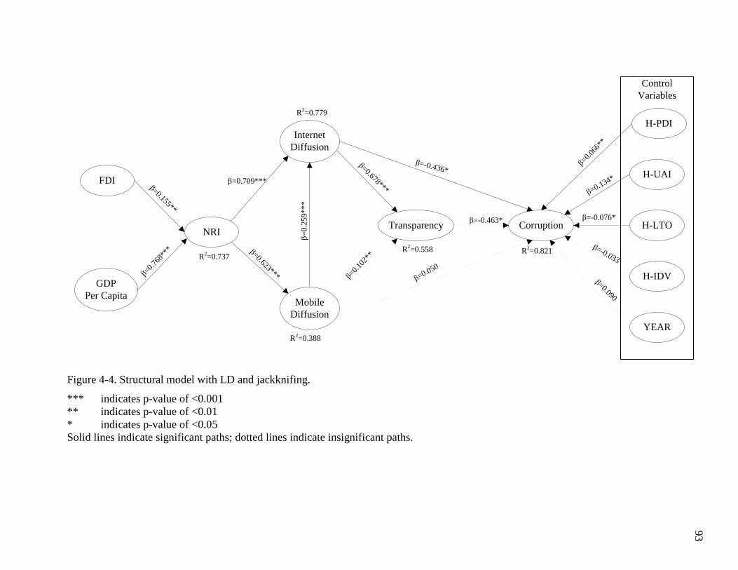
93
FDI
NRI
Internet
Diffusion
Mobile
Diffusion
Transparency Corruption
β=0.155**
β=0.709***
β=0.623***
β=
0.2
59***
β=0.
102*
*
β=0.050
β=-0.463*
β=0.678***
β=-0.436*
H-PDI
H-UAI
H-LTO
H-IDVGDP
Per Capita
YEAR
Control
Variables
β=0.
768*
**R2=0.737
β=0.090
β=-0.033
β=-0.076*
β=0.134*
β=0.
066*
*
R2=0.388
R2=0.779
R2=0.558 R2=0.821
Figure 4-4. Structural model with LD and jackknifing.
*** indicates p-value of <0.001
** indicates p-value of <0.01
* indicates p-value of <0.05
Solid lines indicate significant paths; dotted lines indicate insignificant paths.

94
94
The WarpPLS 3.0 software manual recommends using “the P values associated with the
most stable [path] coefficients” (Kock, 2012, p. 13). The significant path coefficients along with the
related P values were estimated for each missing data treatment and bootstrapping and jackknifing
resampling techniques as shown in Table 4-4.
Table 4-4. Number of significant paths by P-value level.
Significance level
Number of significant paths
RMS LD
bootstrapping jackknifing bootstrapping jackknifing
P<0.05 11 9 10 10
P<0.01 10 6 10 7
P<0.001 9 6 7 5
As predicted by the WarpPLS 3.0 manual, results with large samples and those that used
bootstrapping resampling gave more stable path coefficients. (Kock, 2012). Consequently, the data
with the RMS missing data treatment and bootstrapping resampling technique demonstrated the
higher number of significant paths with stronger associated P values, indicating a higher overall
predictive and explanatory quality of this particular model.
4.3 Model Fit Indices
WarpPLS 3.0 conducts a model fitness test as part of its structural model analysis. The
results of these model fitness tests are outlined in this section. The following model fitness tests
indices were calculated: average path coefficient (APC), average R-squared value (ARS), and
average variance inflation factor (AVIF). The APC index is the average of the absolute values of
the model’s path coefficients. ARS index is the absolute value of the R2 coefficients for the model.

95
95
The AVIF index is the overall measure of multicollinearity of the model. Model fit indices are
useful when comparing the quality of a model with different data. In this study, the quality of the
model was assessed by comparing the APC, ARS, and AVIF values of the data using different
missing data treatments. The ARS and AVIF indices are more important when comparing models
(Kock, 2011b, 2012).
The results of the model fitness tests along with associated P-values are shown in Table 4.3.
It is recommended that APC and ARS are significant at the P<0.05 level and AVIF is less than 5
(Hair et al., 2010; Kline, 2010; Kock, 2012). The APC and ARS indices’ P-values for the data with
both missing data treatments were significant at the P<.001 level. The AVIF index for the data with
both missing data treatments was less than 5. The model using data with the RMS missing data
treatment demonstrated a higher ARS. This indicated that the study’s model had more explanatory
power using data with the RMS treatment. The data with the LD missing data treatment had a
slightly lower AVIF index (1.953) than the data with the RMS missing data treatment (2.145).
However, these AVIF indices had values below the recommended threshold.
Table 4-5. Model fit indices with associated P-values.
Fit Index Data with LD Data with RMS
APC 0.309* 0.300*
ARS 0.657* 0.664*
AVIF 1.953 2.145
Note: * indicates P-value < 0.001

96
96
4.4 Hypotheses Testing
The ARS values for data using the RMS missing data treatment were higher than the LD
missing data treatment as shown in Table 4-5. Also, the data using the RMS missing data treatment
and bootstrapping resampling demonstrated the higher number of significant paths with stronger
associated P values. Given these results of the model fit and significant path tests, data with the
RMS missing data treatment and bootstrapping resampling were used in the hypotheses testing. The
results of the hypotheses testing are presented in Table 4-6. A detailed review of these results for
each hypothesis follows.
Table 4-6: Summary results of hypotheses testing
Hypotheses Supported
H1a: FDI has a positive effect on networked readiness. Accept(a)
H1b: GDP per capita has a positive effect on networked readiness. Accept(a)
H2a: Networked readiness has a positive effect on Internet diffusion. Accept(a)
H2b: Networked readiness has a positive effect on mobile phone diffusion. Accept(a)
H2c: Mobile phone diffusion has a positive effect on Internet diffusion. Accept(a)
H3a: Internet diffusion has a positive effect on transparency. Accept(a)
H3b: Mobile phone diffusion has a positive effect on transparency. Reject
H4a: Internet diffusion has a negative effect on corruption. Accept
H4b: Transparency has a negative effect on corruption. Accept
H4c: Mobile phone diffusion has a negative effect on corruption. Accept
Note: (a) Results significant at P<0.01 across all missing data treatments and resampling analyses.
Hypothesis 1a stated that foreign direct investment (FDI) has a positive effect on networked
readiness (NRI). The results showed that FDI has a significant (P<0.001) and positive (β=0.179)
effect on NRI. Thus, Hypothesis 1a was supported. Figure 4-5 shows the relationship between FDI
and NRI in the data. As shown, the relationship between FDI and NRI was non-linear. WarpPLS
3.0 denoted such relationships as “warped” (Kock, 2012, p. 47). Such relationships are known as U-

97
97
, J- or Kuznet-curves depending on the direction of the curve and the amount of non-linearity
(Selden & Song, 1995). These non-linear relationships have been found in other studies related to
FDI and international trade (D. K. Backus, Kehoe, & Kydland, 1994; Rose & Yellen, 1989).
Figure 4-5. Relationship between FDI and NRI.
Hypothesis 1b stated that GDP per capita, as measured in current US dollars from gross
domestic product per capita (current US$) indicator through the World Bank World Development
Indicators, has a positive effect on networked readiness. GDP per capita had a significant (P<0.001)
and positive (β=0.750) effect on corruption, as measured through the Corruption Perceptions Index

98
98
(CPI) from Transparency International. Thus, Hypothesis 1b was supported. Figure 4-6 shows the
relationship between GDP per capita and NRI in the data. As shown, this relationship was non-
linear.
Figure 4-6. Relationship between GDP per capita and NRI
Hypothesis 2a stated that networked readiness (NRI) has a positive effect on Internet
diffusion as measured through World Bank World Development Internet users (per 100 people)
indicator. The results showed that NRI had a significant (P<0.001) and positive (β=0.578) effect on

99
99
Internet diffusion. Thus, Hypothesis 2 was supported. Figure 4-7 shows the relationship between
NRI and Internet diffusion in the data. As shown, this relationship was relatively linear.
Figure 4-7. Relationship between NRI and Internet diffusion.
Hypothesis 2b stated that networked readiness (NRI) has a positive effect on mobile phone
diffusion (Mobile diffusion). The results showed that NRI had significant (P<0.001) and positive
(β=0.687) effects on mobile diffusion as measured through World Bank World Development
Mobile cellular subscriptions (per 100 people) indicator. Thus, Hypothesis 2b was supported.
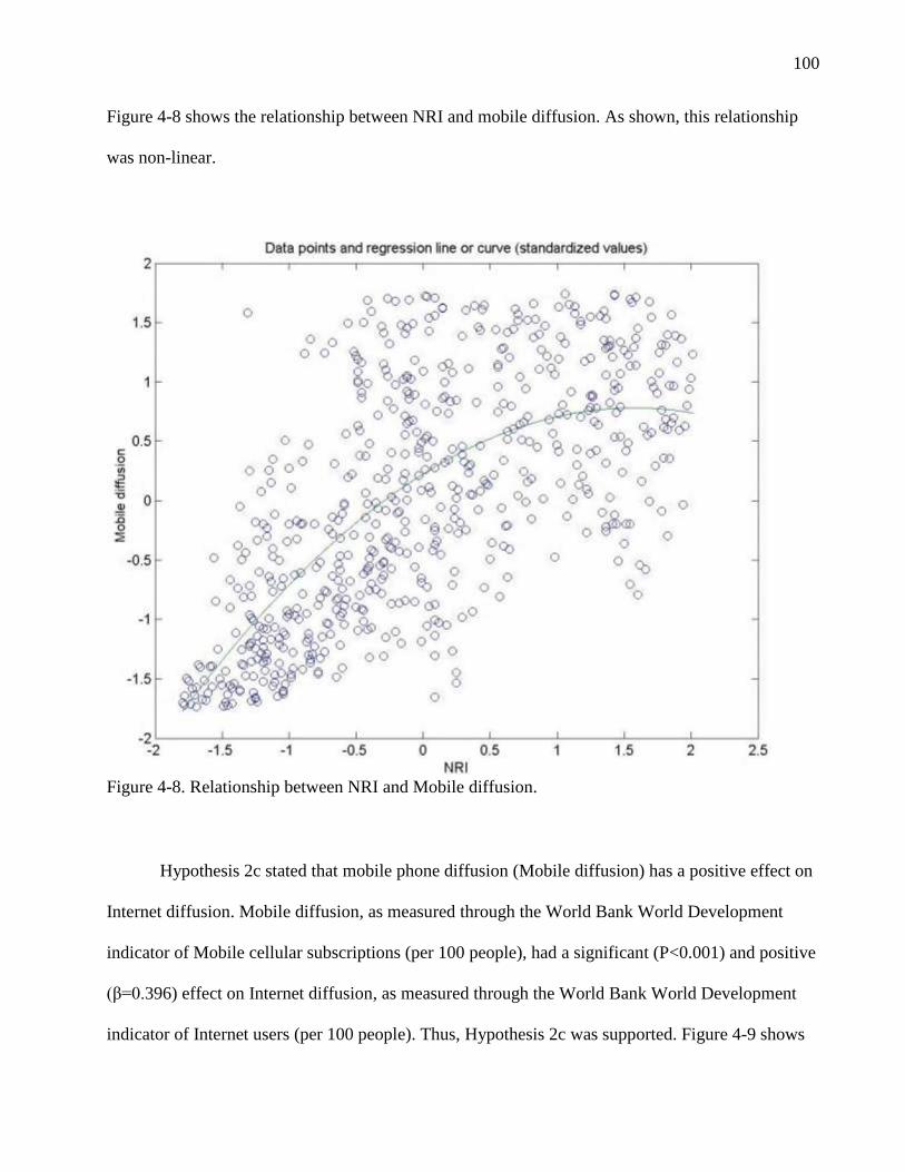
100
10
Figure 4-8 shows the relationship between NRI and mobile diffusion. As shown, this relationship
was non-linear.
Figure 4-8. Relationship between NRI and Mobile diffusion.
Hypothesis 2c stated that mobile phone diffusion (Mobile diffusion) has a positive effect on
Internet diffusion. Mobile diffusion, as measured through the World Bank World Development
indicator of Mobile cellular subscriptions (per 100 people), had a significant (P<0.001) and positive
(β=0.396) effect on Internet diffusion, as measured through the World Bank World Development
indicator of Internet users (per 100 people). Thus, Hypothesis 2c was supported. Figure 4-9 shows
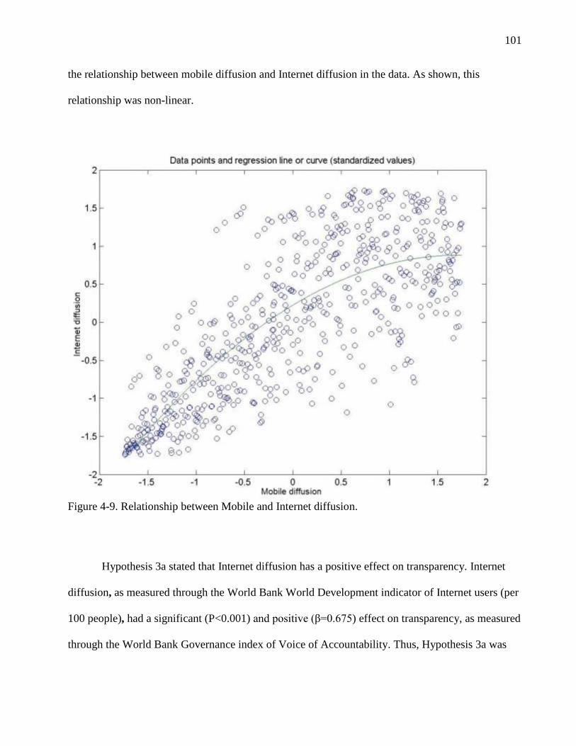
101
10
the relationship between mobile diffusion and Internet diffusion in the data. As shown, this
relationship was non-linear.
Figure 4-9. Relationship between Mobile and Internet diffusion.
Hypothesis 3a stated that Internet diffusion has a positive effect on transparency. Internet
diffusion, as measured through the World Bank World Development indicator of Internet users (per
100 people), had a significant (P<0.001) and positive (β=0.675) effect on transparency, as measured
through the World Bank Governance index of Voice of Accountability. Thus, Hypothesis 3a was

102
10
supported. Figure 4-10 shows the relationship between Internet diffusion and transparency in the
data. As shown, this relationship was non-linear.
Figure 4-10. Relationship between Internet diffusion and transparency.
Hypothesis 3b stated that mobile phone diffusion (Mobile diffusion) had a positive effect on
transparency. Mobile diffusion, as measured through the World Bank World Development indicator
of Mobile cellular subscriptions (per 100 people), did not have a significant (P=0.182) or positive
(β=-0.055) effect on transparency, as measured through the World Bank Governance index of
Voice of Accountability. Thus, Hypothesis 3b was not supported. Figure 4-11 shows the

103
10
relationship between mobile diffusion and transparency in the data using group-mean substitution
with bootstrapping resampling. As shown, this relationship was non-linear.
Figure 4-11. Relationship between mobile diffusion and transparency.
Hypothesis 4a stated that Internet diffusion has a negative effect on corruption. Internet
diffusion, as measured through the World Bank World Development indicator of Internet users (per
100 people), had a significant (P<0.001) and negative (β=-0.410) effect on corruption as measured
through the Corruption Perceptions Index (CPI) from Transparency International. Thus, Hypothesis

104
10
4a was supported. Figure 4-12 shows the relationship between Internet diffusion and corruption in
the data. As shown, this relationship was non-linear.
Figure 4-12. Relationship between Internet diffusion and corruption.
Hypothesis 4b stated that transparency has a negative effect on corruption. Transparency, as
measured through the World Bank Governance index of Voice of Accountability, had a significant
(P<0.001) and negative (β=-0.408) effect on corruption, as measured through the Corruption
Perceptions Index (CPI) from Transparency International. Thus, Hypothesis 4b was supported.

105
10
Figure 4-13 shows the relationship between transparency and corruption in the data. As shown, this
relationship was a non-linear or J-curve.
Figure 4-13. Relationship between transparency and corruption.
Hypothesis 4c stated that mobile phone diffusion (Mobile diffusion) has a negative effect on
corruption. Mobile diffusion, as measured through the World Bank World Development indicator
of Mobile cellular subscriptions (per 100 people), did have a significant (P<0.05) and negative (β=-
0.092) effect on corruption, as measured through the Corruption Perceptions Index (CPI) from
Transparency International. Thus, Hypothesis 4c was supported. Figure 4-14 shows the relationship

106
10
between mobile phone diffusion and corruption in the data. As shown, this relationship was non-
linear.
Figure 4-14. Relationship between mobile diffusion and corruption.
In this study, four control variables were used as national culture control variables to
examine potential cultural factors influencing the main dependent variable. These four national
culture control variables included the Hofstede Cultural Dimension indices of Power Distance,
Individualism vs. Collectivism, Long- vs. Short-Term Orientation, and Uncertainty Avoidance. The

107
10
year was also used as a control variable in order to control for potential multiple year effects. The
year variable did not prove statistically significant (β=0.081, P=0.190) in the data analysis.
The national culture control variable of H-PDI represented the Hofstede Cultural Dimension
of power distance. H-PDI had a significant (P<0.01) and positive (β=0.065) effect on corruption as
measured through the Corruption Perceptions Index (CPI) from Transparency International. The
national culture control variable of H-UAI represented the Hofstede Cultural Dimension of
uncertainty avoidance. H-UAI had a significant (P<0.01) and positive (β=0.085) effect on
corruption as measured through the Corruption Perceptions Index (CPI) from Transparency
International.
The national culture control variable of H-IDV represented the Hofstede Cultural
Dimension of Individualism vs. Collectivism. H-IDV did not have a significant (P=0.447, β=-
0.003) effect on corruption as measured through the Corruption Perceptions Index (CPI) from
Transparency International. The national culture control variable of H-LTO represented the
Hofstede Cultural Dimension of Long- vs. Short-Term Orientation. H-LTO did not have a
significant (P=0.072, β=-0.031) effect on corruption as measured through the Corruption
Perceptions Index (CPI) from Transparency International.
4.4 Direct, Indirect and Total Effects
The J. Cohen (1988) f-squared effect size coefficients were calculated for the paths in this
study’s model. Direct, indirect and total effect coefficients were calculated using WarpPLS 3.0.
Calculation of such indirect, direct and total effect coefficients can prove crucial to evaluating and
explaining mediating effects of variables in the model. Effect size is the contribution by a predictor
variable on the R2 coefficient of a criterion variable.

108
10
WarpPLS 3.0 calculates these effects for variables linked by one or more paths in the
following manner: “the path coefficients associated with the effects, the number of paths that make
up the effects, the P values associated with effects (calculated via resampling, using the selected
resampling method), the standard errors associated with the effects, and effect sizes associated with
the effects” (Kock, 2012, p. 50). According to J. Cohen (1988), effect sizes can be small (0.02),
medium (0.15), or large (0.35). Effect size coefficients (ƒ2) below 0.02 are considered too small for
relevancy.
Direct effects for each variable relationship in the model along with the effect size with
respective P values and standard error are shown in Table 4-7. Direct effects are analogous to the
path coefficients for each variable-to-variable relationship. It is important to note effect size when
examining direct effects. While a direct effect may be significant (P<0.001), magnitude of that
effect (i.e. effect size) may be small. FDI showed a positive and significant direct effect on NRI
(direct effect=0.179, P<0.001). The magnitude of the direct effect of FDI on NRI was small (effect
size=0.104). GDP per capita showed a positive and significant direct effect on NRI (direct
effect=0.750, P<0.001). The magnitude of the direct effect of GDP per capita on NRI was large
(effect size=0.634).
NRI showed a positive and significant direct effect on Internet diffusion (direct
effect=0.578, P<0.001). The magnitude of the direct effect of NRI on Internet diffusion was large
(effect size=0.491). NRI showed a positive and significant direct effect on Mobile diffusion (direct
effect=0.678, P<0.001). The magnitude of the direct effect of NRI on Mobile diffusion was large
(effect size=0.472). Mobile diffusion showed a positive and significant direct effect on Internet
diffusion (direct effect=0.396, P<0.001). The magnitude of the direct effect of Mobile diffusion on
Internet diffusion was medium (effect size=0.314). Mobile diffusion showed a negative but not

109
10
significant direct effect on Transparency (direct effect=-0.055, p=0.182). The magnitude of the
direct effect of Mobile diffusion on Transparency was small (effect size=0.028). Mobile diffusion
showed a negative and significant direct effect on Corruption (direct effect=-0.092, P<0.05,
p=0.015). The magnitude of the direct effect of Mobile diffusion on Corruption was small (effect
size=0.053).
Internet diffusion showed a positive and significant direct effect on Transparency (direct
effect=0.675, P<0.001). The magnitude of the direct effect of Internet diffusion on Transparency
was large (effect size=0.481). Internet diffusion showed a positive and significant direct effect on
Corruption (direct effect=-0.410, P<0.001). The magnitude of the direct effect of Internet diffusion
on Corruption was medium (effect size=0.348). Transparency showed a negative and significant
direct effect on Corruption (direct effect=-0.408, P<0.001). The magnitude of the direct effect of
Transparency on Corruption was medium (effect size=0.348).
The control variables were also analyzed for their direct effect on Corruption. Hofstede’s
power distance index (H-PDI) showed a positive and significant direct effect on Corruption (direct
effect=0.065, P<0.01, p=0.008). The magnitude of the direct effect of H-PDI on Corruption was
small (effect size=0.045). Hofstede’s uncertainty avoidance index (H-UAI) showed a positive and
significant direct effect on Corruption (direct effect=0.085, P<0.01, p=0.002). The magnitude of the
direct effect of H-UAI on Corruption was small (effect size=0.045). Hofstede’s long-term
orientation (H-LTO) showed a negative but not significant direct effect on Corruption (direct
effect=-0.031, p=0.072). The magnitude of the direct effect of H-LTO on Corruption was below
Cohen’s recommended effect size threshold for relevancy (effect size=0.008). Hofstede’s
individuality index (H-IDV) showed a negative but not significant direct effect on Corruption

110
11
(direct effect=-0.003, p=0.447). The magnitude of the direct effect of H-IDV on Corruption was
below Cohen’s recommended effect size threshold for relevancy (effect size=0.002).
Table 4-7. Direct effects for each variable relationship.
Relationship Total
Effect P-value
Effect Size
Coefficient*
Effect
Size* Std. Err.
FDI → NRI 0.179 <0.001 0.104 small 0.030
GDP per capita → NRI 0.750 <0.001 0.634 large 0.025
NRI → Internet diffusion 0.578 <0.001 0.491 large 0.023
NRI → Mobile diffusion 0.687 <0.001 0.472 large 0.018
Mobile diffusion → Internet
diffusion 0.396 <0.001 0.314 medium 0.026
Mobile diffusion → Transparency -0.055 0.182 0.028 small 0.061
Mobile diffusion → Corruption -0.092 0.015 0.053 small 0.042
Internet diffusion → Transparency 0.675 <0.001 0.481 large 0.028
Internet diffusion → Corruption -0.410 <0.001 0.347 medium 0.061
Transparency → Corruption -0.408 <0.001 0.348 medium 0.061
H-PDI → Corruption 0.065 0.008 0.045 small 0.027
H-UAI → Corruption 0.085 0.002 0.024 small 0.030
H-LTO → Corruption -0.031 0.072 0.008 no rel. 0.021
H-IDV → Corruption -0.003 0.447 0.002 no rel. 0.025
Note: * Effect size coefficients and effect size are reported. According to J. Cohen (1988), effect
sizes can be small (0.02), medium (0.15), or large (0.35). Effect size coefficients below 0.02 are
considered too small for relevancy (no rel.).
Indirect effects are introduced when the path from an initial variable to an outcome variable
has other intervening variables. The intervening variables in a model can have a mediation effect on
the relationship between the initial and outcome variables. The indirect effects by number of
aggregated segments and summation of indirect effects for each variable relationship in the model
along with the effect size with respective P values and standard error were also calculated.
The indirect effects of initial variables on outcome variables with two aggregated segments,
along with associate P values, effect size, and standard errors are shown in Table 4-8. Internet
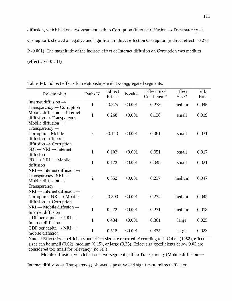
111
11
diffusion, which had one two-segment path to Corruption (Internet diffusion → Transparency →
Corruption), showed a negative and significant indirect effect on Corruption (indirect effect=-0.275,
P<0.001). The magnitude of the indirect effect of Internet diffusion on Corruption was medium
(effect size=0.233).
Table 4-8. Indirect effects for relationships with two aggregated segments.
Relationship Paths N Indirect
Effect P-value
Effect Size
Coefficient*
Effect
Size*
Std.
Err.
Internet diffusion →
Transparency → Corruption 1 -0.275 <0.001 0.233 medium 0.045
Mobile diffusion → Internet
diffusion → Transparency 1 0.268 <0.001 0.138 small 0.019
Mobile diffusion →
Transparency →
Corruption; Mobile
diffusion → Internet
diffusion → Corruption
2 -0.140 <0.001 0.081 small 0.031
FDI → NRI → Internet
diffusion 1 0.103 <0.001 0.051 small 0.017
FDI → NRI → Mobile
diffusion 1 0.123 <0.001 0.048 small 0.021
NRI → Internet diffusion →
Transparency; NRI →
Mobile diffusion →
Transparency
2 0.352 <0.001 0.237 medium 0.047
NRI → Internet diffusion →
Corruption; NRI → Mobile
diffusion → Corruption
2 -0.300 <0.001 0.274 medium 0.045
NRI → Mobile diffusion →
Internet diffusion 1 0.272 <0.001 0.231 medium 0.018
GDP per capita → NRI →
Internet diffusion 1 0.434 <0.001 0.361 large 0.025
GDP per capita → NRI →
mobile diffusion 1 0.515 <0.001 0.375 large 0.023
Note: * Effect size coefficients and effect size are reported. According to J. Cohen (1988), effect
sizes can be small (0.02), medium (0.15), or large (0.35). Effect size coefficients below 0.02 are
considered too small for relevancy (no rel.).
Mobile diffusion, which had one two-segment path to Transparency (Mobile diffusion →
Internet diffusion → Transparency), showed a positive and significant indirect effect on

112
11
Transparency (indirect effect=0.268, P<0.001). The magnitude of the indirect effect of Mobile
diffusion on Transparency was small (effect size=0.138). Mobile diffusion, which had two two-
segment path to Corruption (Mobile diffusion → Transparency → Corruption; Mobile diffusion →
Internet diffusion → Corruption), showed a negative and significant indirect effect on Corruption
(indirect effect=-0.140, P<0.001). The magnitude of the indirect effect of Mobile diffusion on
Corruption was small (effect size=0.081). FDI, which had one two-segment path to Internet
diffusion (FDI → NRI → Internet diffusion), showed a positive and significant indirect effect on
Internet diffusion (indirect effect=0.103, P<0.001). The magnitude of the indirect effect of FDI on
Internet diffusion was small (effect size=0.051).
FDI, which had one two-segment path to Mobile diffusion (FDI → NRI → Mobile
diffusion), showed a positive and significant indirect effect on mobile diffusion (indirect
effect=0.123, P<0.001). The magnitude of the indirect effect of FDI on Mobile diffusion was small
(effect size=0.048). NRI, which had two two-segment path to Transparency (NRI → Internet
diffusion → Transparency; NRI → Mobile diffusion → Transparency), showed a positive and
significant indirect effect on Transparency (indirect effect=0.352, P<0.001). The magnitude of the
indirect effect of NRI on Transparency was medium (effect size=0.237). NRI, which had two two-
segment path to Corruption (NRI → Internet diffusion → Corruption; NRI → Mobile diffusion →
Corruption), showed a negative and significant indirect effect on Corruption (indirect effect=-0.300,
P<0.001). The magnitude of the indirect effect of NRI on Corruption was medium (effect
size=0.274). NRI, which had one two-segment path to Internet diffusion (NRI → Mobile diffusion
→ Internet diffusion), showed a positive and significant indirect effect on Internet diffusion
(indirect effect=0.272, P<0.001). The magnitude of the indirect effect of NRI on Internet diffusion
was medium (effect size=0.231). GDP per capita, which had one two-segment path to Internet

113
11
diffusion (GDP per capita → NRI → Internet diffusion), showed a positive and significant indirect
effect on Internet diffusion (indirect effect=0.434, P<0.001). The magnitude of the indirect effect of
GDP per capita on Internet diffusion was large (effect size=0.361). GDP per capita, which had one
two-segment path to Mobile diffusion (GDP per capita → NRI → Mobile diffusion), showed a
positive and significant indirect effect on Mobile diffusion (indirect effect=0.515, P<0.001). The
magnitude of the indirect effect of GDP per capita on Mobile diffusion was large (effect
size=0.375).
The indirect effects of initial variables on outcome variables with three aggregated
segments, along with associate P values, effect size, and standard errors are shown in Table 4-9.
Mobile diffusion, which had one three-segment path to Corruption (Mobile diffusion → Internet
diffusion → Transparency → Corruption), showed a negative and significant indirect effect on
Corruption (indirect effect=-0.109, P<0.001). The magnitude of the indirect effect of Mobile
diffusion on Corruption was small (effect size=0.063).
FDI, which had two three-segment path to Transparency (FDI → NRI → Internet diffusion
→ Transparency; FDI → NRI → Mobile diffusion → Transparency), showed a positive and
significant indirect effect on Transparency (indirect effect=0.063, P<0.001). The magnitude of the
indirect effect of FDI on Transparency was small (effect size=0.021). FDI, which had two three-
segment path to Corruption (FDI → NRI → Internet diffusion → Corruption; FDI → NRI →
Mobile diffusion → Corruption), showed a negative and significant indirect effect on Corruption
(indirect effect=-0.054, P<0.001). The magnitude of the indirect effect of FDI on Corruption was
small (effect size=0.026).

114
11
Table 4-9. Indirect effects for relationships with three aggregated segments.
Relationship (aggregate
paths) Paths N
Indirect
Effect
P-
value
Effect Size
Coefficient*
Effect
Size*
Std.
Err.
Mobile diffusion →
Internet diffusion →
Transparency →
Corruption
1 -0.109 <0.001 0.063 small 0.020
FDI → NRI → Internet
diffusion → Transparency;
FDI → NRI → Mobile
diffusion → Transparency
2 0.063 <0.001 0.021 small 0.013
FDI → NRI → Internet
diffusion → corruption;
FDI → NRI → mobile
diffusion → corruption
2 -0.054 <0.001 0.026 small 0.012
FDI → NRI → Mobile
diffusion → Internet
diffusion
1 0.049 <0.001 0.024 small 0.010
NRI → Mobile diffusion
→ Internet diffusion →
Transparency
1 0.184 <0.001 0.124 small 0.014
NRI → Mobile diffusion
→ Transparency →
Corruption; NRI →
Internet diffusion →
Transparency →
Corruption; NRI → Mobile
diffusion → Internet
diffusion → Corruption
3 -0.256 <0.001 0.233 medium 0.025
GDP per capita → NRI →
Mobile diffusion →
Transparency; GDP per
capita → NRI → Internet
diffusion→ Transparency
2 0.264 <0.001 0.186 medium 0.038
GDP per capita → NRI →
Mobile diffusion →
Corruption; GDP per capita
→ NRI → Internet
diffusion → Corruption
2 -0.225 <0.001 0.193 medium 0.033
GDP per capita → NRI →
Mobile diffusion →
Internet diffusion
1 0.204 <0.001 0.170 medium 0.014
Note: * Effect size coefficients and effect size are reported. According to J. Cohen (1988),
effect sizes can be small (0.02), medium (0.15), or large (0.35). Effect size coefficients below
0.02 are considered too small for relevancy (no rel.).

115
11
FDI, which had one three-segment path to Internet diffusion (FDI → NRI → Mobile
diffusion → Internet diffusion), showed a negative and significant indirect effect on Internet
diffusion (indirect effect=-0.049, P<0.001). The magnitude of the indirect effect of FDI on Internet
diffusion was small (effect size=0.024). NRI, which had one three-segment path to Transparency
(NRI → mobile diffusion → Internet diffusion → Transparency), showed a positive and significant
indirect effect on Transparency (indirect effect=0.184, P<0.001). The magnitude of the indirect
effect of NRI on Transparency was small (effect size=0.124). NRI, which had three three-segment
path to Corruption (NRI → Mobile diffusion → Transparency → Corruption; NRI → Internet
diffusion → Transparency → Corruption; NRI → Mobile diffusion → Internet diffusion →
Corruption), showed a negative and significant indirect effect on Corruption (indirect effect=-0.256,
P<0.001). The magnitude of the indirect effect of NRI on corruption was medium (effect
size=0.233). GDP per capita, which had two three-segment path to Transparency (GDP per capita
→ NRI → Mobile diffusion → Transparency; GDP per capita → NRI → Internet diffusion→
Transparency), showed a positive and significant indirect effect on Transparency (indirect
effect=0.264, P<0.001). The magnitude of the indirect effect of GDP per capita on Transparency
was medium (effect size=0.186). GDP per capita, which had two three-segment path to Corruption
(GDP per capita → NRI → Mobile diffusion → Corruption; GDP per capita → NRI → Internet
diffusion → Corruption), showed a negative and significant indirect effect on Corruption (indirect
effect=-0.225, P<0.001). The magnitude of the indirect effect of GDP per capita on Corruption was
medium (effect size=0.193). GDP per capita, which had one three-segment path to Internet
diffusion (GDP per capita → NRI → Mobile diffusion → Internet diffusion), showed a negative
and significant indirect effect on Internet diffusion (indirect effect=0.204, P<0.001). The magnitude
of the indirect effect of GDP per capita on Internet diffusion was medium (effect size=0.170).

116
11
The indirect effects of initial variables on outcome variables with four aggregated segments,
along with associate P values, effect size, and standard errors are shown in Table 4-10.
Table 4-10. Indirect effects for relationships with four aggregated segments.
Relationship (aggregate
paths)
Paths
N
Indirect
Effect P-value
Effect Size
Coefficient*
Effect
Size*
Std.
Err.
FDI → NRI → Mobile
diffusion → Internet
diffusion → Transparency
1 0.033 <0.001 0.011 no rel. 0.006
FDI → NRI → Mobile
diffusion → Internet
diffusion → Corruption; FDI
→ NRI → Mobile diffusion
→ Transparency →
Corruption; FDI → NRI →
Mobile diffusion →
Transparency → Corruption
3 -0.046 <0.001 0.022 small 0.008
NRI → Mobile diffusion →
Internet diffusion →
Transparency→ Corruption
1 -0.075 <0.001 0.069 small 0.013
GDP per capita → NRI →
Mobile diffusion → Internet
diffusion → Transparency
1 0.138 <0.001 0.097 small 0.011
GDP per capita → NRI →
Mobile diffusion → Internet
diffusion → Corruption;
GDP per capita → NRI →
Mobile diffusion →
Transparency → Corruption;
GDP per capita → NRI →
Internet diffusion →
Transparency →Corruption
3 -0.192 <0.001 0.164 medium 0.021
Note: * Effect size coefficients and effect size are reported. According to J. Cohen (1988), effect
sizes can be small (0.02), medium (0.15), or large (0.35). Effect size coefficients below 0.02 are
considered too small for relevancy (no rel.).
FDI, which had one four-segment path to Transparency (FDI → NRI → Mobile diffusion
→ Internet diffusion → Transparency), showed a positive and significant indirect effect on

117
11
Transparency (indirect effect=0.033, P<0.001). The magnitude of the indirect effect of FDI on
Transparency was below Cohen’s recommended effect size threshold for relevancy (effect
size=0.011). FDI, which had three four-segment path to Corruption (FDI → NRI → Mobile
diffusion → Internet diffusion → Corruption; FDI → NRI → Mobile diffusion → transparency →
Corruption; FDI → NRI → Mobile diffusion → Transparency → Corruption), showed a negative
and significant indirect effect on Corruption (indirect effect=-0.046, P<0.001). The magnitude of
the indirect effect of FDI on Corruption was small (effect size=0.022).
NRI, which had one four-segment path to Corruption (NRI → Mobile diffusion → Internet
diffusion → Transparency→ Corruption), showed a negative and significant indirect effect on
Corruption (indirect effect=0.033, P<0.001). The magnitude of the indirect effect of NRI on
Corruption was small (effect size=0.069). GDP per capita, which had one four-segment path to
Transparency (GDP per capita → NRI → Mobile diffusion → Internet diffusion → Transparency),
showed a positive and significant indirect effect on Transparency (indirect effect=0.138, P<0.001).
The magnitude of the indirect effect of GDP per capita on Transparency was small (effect
size=0.097). GDP per capita, which had three four-segment path to Corruption (GDP per capita →
NRI → Mobile diffusion → Internet diffusion → Corruption; GDP per capita → NRI → Mobile
diffusion → Transparency → Corruption; GDP per capita → NRI → Internet diffusion →
Transparency →Corruption), showed a negative and significant indirect effect on Corruption
(indirect effect=-0.192, P<0.001). The magnitude of the indirect effect of GDP per capita on
Corruption was medium (effect size=0.164).
The indirect effects of initial variables on outcome variables with five aggregated segments,
along with associate P values, effect size, and standard errors are shown in Table 4-11. FDI, which
had one five-segment path to Corruption (FDI → NRI → Mobile diffusion → Internet diffusion →

118
11
Transparency → Corruption), showed a negative and significant indirect effect on Corruption
(indirect effect=-0.013, P<0.001). The magnitude of the indirect effect of FDI on corruption was
below Cohen’s recommended effect size threshold for relevancy (effect size=0.007). GDP per
capita, which had one five-segment path (GDP per capita → NRI → Mobile diffusion → Internet
diffusion → Transparency → Corruption), showed a negative and significant indirect effect on
Corruption (indirect effect=-0.013, P<0.001). The magnitude of the indirect effect of GDP per
capita on Corruption was below Cohen’s recommended effect size threshold for relevancy (effect
size=0.007).
Table 4-11. Indirect effects for relationships with five aggregated segments.
Relationship (aggregate
paths) Paths N
Indirect
Effect P-value
Effect Size
Coefficient*
Effect
Size*
Std.
Err.
FDI → NRI → Mobile
diffusion → Internet
diffusion → Transparency
→ Corruption
1 -0.013 <0.001 0.007 no rel. 0.003
GDP per capita → NRI →
Mobile diffusion →
Internet diffusion →
Transparency →
Corruption
1 -0.056 <0.001 0.048 small 0.011
Note: * Effect size coefficients and effect size are reported. According to J. Cohen (1988),
effect sizes can be small (0.02), medium (0.15), or large (0.35). Effect size coefficients below
0.02 are considered too small for relevancy (no rel.).
The sum of indirect effects of initial variables on outcome variables in the model, along with
the number of paths, the effect size with respective P values and standard error are shown in Table
4-12. Internet diffusion, which had one path to Corruption (Internet diffusion → Corruption),
showed a negative and significant indirect effect on Corruption (sum of indirect effect=-0.275,

119
11
P<0.001). The summative magnitude of the indirect effect of Internet diffusion on Corruption was
medium (effect size=0.233).
Table 4-12. Sum of indirect effects.
Relationship Paths N Indirect
Effect P-value
Effect Size
Coefficient*
Effect
Size*
Std.
Err.
Internet diffusion →
Corruption 1 -0.275 <0.001 0.233 medium 0.045
Mobile diffusion →
Transparency 1 0.268 <0.001 0.138 small 0.019
Mobile diffusion →…→
Corruption 3 -0.249 <0.001 0.144 small 0.033
FDI → …→
Transparency 3 0.096 <0.001 0.032 small 0.019
FDI → …→ Corruption 6 -0.113 <0.001 0.055 small 0.033
FDI →… → Internet
diffusion 2 0.152 <0.001 0.075 small 0.019
FDI → Mobile diffusion 1 0.123 <0.001 0.048 small 0.033
NRI → …→
Transparency 3 0.536 <0.001 0.361 large 0.048
NRI → …→ Corruption 6 -0.631 <0.001 0.576 large 0.033
NRI → Internet diffusion 1 0.272 <0.001 0.231 medium 0.018
GDP per capita →… →
Transparency 3 0.402 <0.001 0.283 medium 0.040
GDP per capita → …→
Corruption 6 -0.473 <0.001 0.406 large 0.029
GDP per capita →…→
Internet diffusion 2 0.638 <0.001 0.530 large 0.024
GDP per capita →
Mobile diffusion 1 0.515 <0.001 0.375 large 0.023
Note: * Effect size coefficients and effect size are reported. According to J. Cohen (1988), effect
sizes can be small (0.02), medium (0.15), or large (0.35). Effect size coefficients below 0.02 are
considered too small for relevancy (no rel.).
Mobile diffusion, which had one path to Transparency (Mobile diffusion → Transparency),
showed a positive and significant indirect effect on Transparency (sum of indirect effect=0.268,
P<0.001). The summative magnitude of the indirect effect of Mobile diffusion on Transparency was

120
12
small (effect size=0.138). Mobile diffusion, which had three paths to Corruption (Mobile diffusion
→ Transparency → Corruption; Mobile diffusion → Internet diffusion → Corruption; Mobile
diffusion → Internet diffusion → Transparency → Corruption), showed a negative and significant
indirect effect on Corruption (sum of indirect effect=-0.249, P<0.001). The summative magnitude
of the indirect effect of Mobile diffusion on Corruption was small (effect size=0.144).
FDI, which had three paths to Transparency (FDI → NRI → Internet diffusion →
Transparency; FDI → NRI → Mobile diffusion → Transparency; FDI → NRI → Mobile diffusion
→ Internet diffusion → Transparency), showed a positive and significant indirect effect on
Transparency (sum of indirect effect=0.096, P<0.001). The summative magnitude of the indirect
effect of FDI on Transparency was small (effect size=0.032). FDI, which had six paths to
Corruption (FDI → NRI → Internet diffusion → Corruption; FDI → NRI → Mobile diffusion →
Corruption; FDI → NRI → Mobile diffusion → Internet diffusion → Corruption; FDI → NRI →
Mobile diffusion → Transparency → Corruption; FDI → NRI → Mobile diffusion →
Transparency → Corruption; FDI → NRI → Mobile diffusion → Internet diffusion →
Transparency → Corruption), showed a negative and significant indirect effect on Corruption (sum
of indirect effect=-0.113, P<0.001). The summative magnitude of the indirect effect of FDI on
Corruption was small (effect size=0.055).
FDI, which had two paths to Internet diffusion (FDI → NRI → Internet diffusion; FDI →
NRI → Mobile diffusion → Internet diffusion), showed a positive and significant indirect effect on
Internet diffusion (sum of indirect effect=0.152, P<0.001). The summative magnitude of the
indirect effect of FDI on Internet diffusion was small (effect size=0.075). FDI, which had one path
to Mobile diffusion (FDI → NRI → Mobile diffusion), showed a positive and significant indirect
effect on Mobile diffusion (sum of indirect effect=0.123, P<0.001). The summative magnitude of

121
12
the indirect effect of FDI on Mobile diffusion was small (effect size=0.048). NRI, which had three
paths to Transparency (NRI → Internet diffusion → Transparency; NRI → Mobile diffusion →
Transparency; NRI → Mobile diffusion → Internet diffusion → Transparency), showed a positive
and significant indirect effect on Transparency (sum of indirect effect=0.536, P<0.001). The
summative magnitude of the indirect effect of NRI on Transparency was large (effect size=0.361).
NRI, which had six paths to Corruption (NRI → Internet diffusion → Corruption; NRI →
Mobile diffusion → Corruption; NRI → Mobile diffusion → Transparency → Corruption; NRI →
Internet diffusion → Transparency → Corruption; NRI → Mobile diffusion → Internet diffusion →
Corruption; NRI → Mobile diffusion → Internet diffusion → Transparency→ Corruption), showed
a negative and significant indirect effect on Corruption (sum of indirect effect=-0.631, P<0.001).
The summative magnitude of the indirect effect of NRI on Corruption was large (effect size=0.576).
NRI, which had one path to Internet diffusion (NRI → Mobile diffusion → Internet diffusion),
showed a positive and significant indirect effect on Internet diffusion (sum of indirect effect=0.272,
P<0.001). The summative magnitude of the indirect effect of NRI on Internet diffusion was medium
(effect size=0.231).
GDP per capita, which had three paths to Transparency (GDP per capita → NRI → Mobile
diffusion → Transparency; GDP per capita → NRI → Internet diffusion→ Transparency; GDP per
capita → NRI → Mobile diffusion → Internet diffusion → Transparency), showed a positive and
significant indirect effect on Transparency (sum of indirect effect=0.402, P<0.001). The summative
magnitude of the indirect effect of GDP per capita on Transparency was medium (effect
size=0.283). GDP per capita, which had six paths to Corruption (GDP per capita → NRI → Mobile
diffusion → Corruption; GDP per capita → NRI → Internet diffusion → Corruption; GDP per
capita → NRI → Mobile diffusion → Internet diffusion → Corruption; GDP per capita → NRI →

122
12
Mobile diffusion → Transparency → Corruption; GDP per capita → NRI → Internet diffusion →
Transparency →Corruption; GDP per capita → NRI → Mobile diffusion → Internet diffusion →
Transparency → Corruption), showed a negative and significant indirect effect on Corruption (sum
of indirect effect=-0.473, P<0.001). The summative magnitude of the indirect effect of GDP per
capita on Corruption was large (effect size=0.406). GDP per capita, which had two paths to Internet
diffusion (GDP per capita → NRI → Internet diffusion; GDP per capita → NRI → Mobile
diffusion → Internet diffusion), showed a positive and significant indirect effect on Internet
diffusion (sum of indirect effect=0.638, P<0.001). The summative magnitude of the indirect effect
of GDP per capita on Internet diffusion was large (effect size=0.530). GDP per capita, which had
one path to Mobile diffusion (GDP per capita → NRI → Mobile diffusion), showed a positive and
significant indirect effect on Mobile diffusion (sum of indirect effect=0.515, P<0.001). The
summative magnitude of the indirect effect of GDP per capita on Mobile diffusion was large (effect
size=0.375).
The total effect of FDI, along with the number of paths, the effect size with respective P
values and standard error are shown in Table 4-13. FDI showed a positive and significant total
effect on Transparency (total effect=0.096, P<0.001). The magnitude of the total effect of FDI on
Transparency was small (effect size=0.032). FDI showed a negative and significant total effect on
Corruption (total effect=-0.113, P<0.001). The magnitude of the total effect of FDI on Corruption
was small (effect size=0.055). FDI showed a positive and significant total effect on Internet
diffusion (total effect=0.152, P<0.001). The magnitude of the total effect of FDI on Internet
diffusion was small (effect size=0.075). FDI showed a positive and significant total effect on
Mobile diffusion (total effect=0.123, P<0.001). The magnitude of the total effect of FDI on Mobile
diffusion was small (effect size=0.048). FDI showed a positive and significant total effect on NRI

123
12
(total effect=0.179, P<0.001). The magnitude of the total effect of FDI on NRI was small (effect
size=0.104).
Table 4-13. Total effect of FDI.
Paths N
Total
Effect P-value
Effect Size
Coefficient*
Effect
Size* Std. Err.
Transparency 3 0.096 <0.001 0.032 small 0.017
Corruption 6 -0.113 <0.001 0.055 small 0.019
Internet
Diffusion 2 0.152 <0.001 0.075 small 0.026
Mobile
Diffusion 1 0.123 <0.001 0.048 small 0.021
NRI 1 0.179 <0.001 0.104 small 0.030
Note: * Effect size coefficients and effect size are reported. According to J. Cohen (1988), effect
sizes can be small (0.02), medium (0.15), or large (0.35). Effect size coefficients below 0.02 are
considered too small for relevancy (no rel.).
The total effect of GDP per capita, along with the number of paths, the effect size with
respective P values, and standard error are shown in Table 4-14. GDP per capita showed a positive
and significant total effect on Transparency (total effect=0.402, P<0.001). The magnitude of the
total effect of GDP per capita on Transparency was medium (effect size=0.283). GDP per capita
showed a negative and significant total effect on Corruption (total effect=-0.473, P<0.001). The
magnitude of the total effect of GDP per capita on Corruption was large (effect size=0.406). GDP
per capita showed a positive and significant total effect on Internet diffusion (total effect=0.638,
P<0.001). The magnitude of the total effect of GDP per capita on Internet diffusion was large
(effect size=0.530). GDP per capita showed a positive and significant total effect on Mobile
diffusion (total effect=0.515, P<0.001). The magnitude of the total effect of GDP per capita on
mobile diffusion was large (effect size=0.375). GDP per capita showed a positive and significant
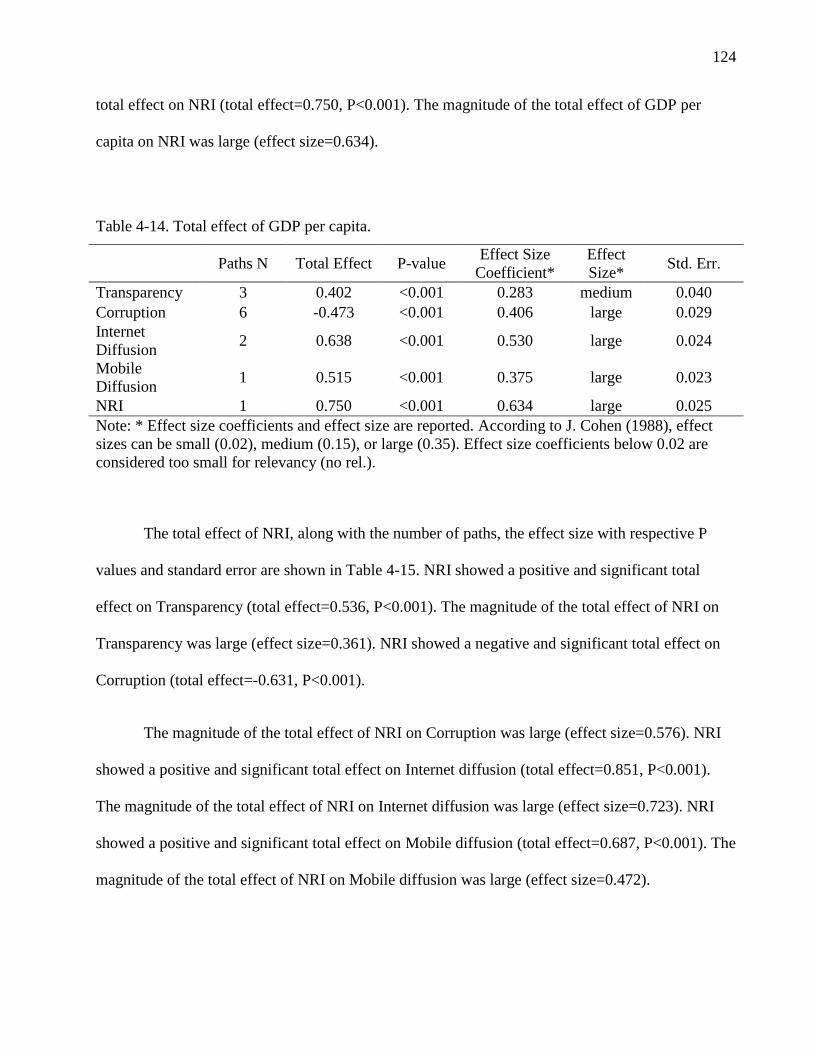
124
12
total effect on NRI (total effect=0.750, P<0.001). The magnitude of the total effect of GDP per
capita on NRI was large (effect size=0.634).
Table 4-14. Total effect of GDP per capita.
Paths N Total Effect P-value
Effect Size
Coefficient*
Effect
Size* Std. Err.
Transparency 3 0.402 <0.001 0.283 medium 0.040
Corruption 6 -0.473 <0.001 0.406 large 0.029
Internet
Diffusion 2 0.638 <0.001 0.530 large 0.024
Mobile
Diffusion 1 0.515 <0.001 0.375 large 0.023
NRI 1 0.750 <0.001 0.634 large 0.025
Note: * Effect size coefficients and effect size are reported. According to J. Cohen (1988), effect
sizes can be small (0.02), medium (0.15), or large (0.35). Effect size coefficients below 0.02 are
considered too small for relevancy (no rel.).
The total effect of NRI, along with the number of paths, the effect size with respective P
values and standard error are shown in Table 4-15. NRI showed a positive and significant total
effect on Transparency (total effect=0.536, P<0.001). The magnitude of the total effect of NRI on
Transparency was large (effect size=0.361). NRI showed a negative and significant total effect on
Corruption (total effect=-0.631, P<0.001).
The magnitude of the total effect of NRI on Corruption was large (effect size=0.576). NRI
showed a positive and significant total effect on Internet diffusion (total effect=0.851, P<0.001).
The magnitude of the total effect of NRI on Internet diffusion was large (effect size=0.723). NRI
showed a positive and significant total effect on Mobile diffusion (total effect=0.687, P<0.001). The
magnitude of the total effect of NRI on Mobile diffusion was large (effect size=0.472).
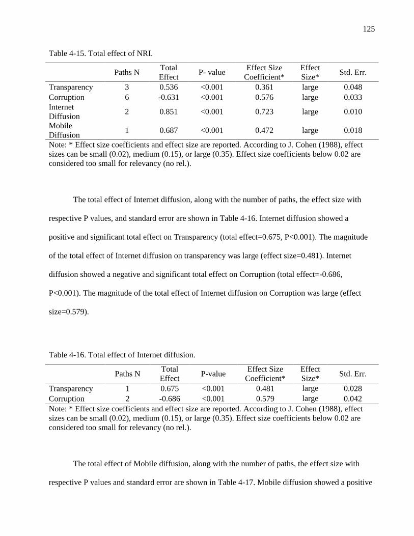
125
12
Table 4-15. Total effect of NRI.
Paths N
Total
Effect P- value
Effect Size
Coefficient*
Effect
Size* Std. Err.
Transparency 3 0.536 <0.001 0.361 large 0.048
Corruption 6 -0.631 <0.001 0.576 large 0.033
Internet
Diffusion 2 0.851 <0.001 0.723 large 0.010
Mobile
Diffusion 1 0.687 <0.001 0.472 large 0.018
Note: * Effect size coefficients and effect size are reported. According to J. Cohen (1988), effect
sizes can be small (0.02), medium (0.15), or large (0.35). Effect size coefficients below 0.02 are
considered too small for relevancy (no rel.).
The total effect of Internet diffusion, along with the number of paths, the effect size with
respective P values, and standard error are shown in Table 4-16. Internet diffusion showed a
positive and significant total effect on Transparency (total effect=0.675, P<0.001). The magnitude
of the total effect of Internet diffusion on transparency was large (effect size=0.481). Internet
diffusion showed a negative and significant total effect on Corruption (total effect=-0.686,
P<0.001). The magnitude of the total effect of Internet diffusion on Corruption was large (effect
size=0.579).
Table 4-16. Total effect of Internet diffusion.
Paths N
Total
Effect P-value
Effect Size
Coefficient*
Effect
Size* Std. Err.
Transparency 1 0.675 <0.001 0.481 large 0.028
Corruption 2 -0.686 <0.001 0.579 large 0.042
Note: * Effect size coefficients and effect size are reported. According to J. Cohen (1988), effect
sizes can be small (0.02), medium (0.15), or large (0.35). Effect size coefficients below 0.02 are
considered too small for relevancy (no rel.).
The total effect of Mobile diffusion, along with the number of paths, the effect size with
respective P values and standard error are shown in Table 4-17. Mobile diffusion showed a positive

126
12
and significant total effect on Transparency (total effect=0.212, P<0.001). The magnitude of the
total effect of Mobile diffusion on Transparency was small (effect size=0.109). Mobile diffusion
showed a negative and significant total effect on Corruption (total effect=-0.341, P<0.001). The
magnitude of the total effect of Mobile diffusion on Corruption was medium (effect size=0.197).
Mobile diffusion showed a positive and significant total effect on Internet diffusion (total
effect=0.396, P<0.001). The magnitude of the total effect of Mobile diffusion on Internet diffusion
was medium (effect size=0.314).
Table 4-17. Total effect of Mobile diffusion.
Paths N
Total
Effect P-value
Effect Size
Coefficient*
Effect
Size* Std. Err.
Transparency 2 0.212 <0.001 0.109 small 0.064
Corruption 4 -0.341 <0.001 0.197 medium 0.044
Internet
Diffusion 1 0.396 <0.001 0.314 medium 0.026
Note: * Effect size coefficients and effect size are reported. According to J. Cohen (1988), effect
sizes can be small (0.02), medium (0.15), or large (0.35). Effect size coefficients below 0.02 are
considered too small for relevancy (no rel.).
The total effect of transparency, along with the number of paths, the effect size with
respective P values and standard error are shown in Table 4-18. Transparency showed a negative
and significant total effect on corruption (total effect=-0.408, P<0.001). The magnitude of the total
effect of transparency on corruption was medium (effect size=0.348).
Table 4-18. Total effect size of Transparency.
Paths N Total Effect P-value
Effect Size
Coefficient* Effect Size* Std. Err.
Corruption 1 -0.408 <0.001 0.348 medium 0.061
Note: * Effect size coefficients and effect size are reported. According to J. Cohen (1988), effect

127
12
sizes can be small (0.02), medium (0.15), or large (0.35). Effect size coefficients below 0.02 are
considered too small for relevancy (no rel.).

128
12
CHAPTER V
DISCUSSION
The purpose of this study was to investigate the effects of the hypothesized relationships of
key macroeconomic, ICT and sociocultural variables on corruption and transparency. Specifically,
this study explored the relationship between the ICT environment, diffusion of specific ICTs (e.g.
Internet diffusion and mobile cellular diffusion), and the two macroeconomic variables of FDI and
Gross Domestic Product (GDP) per capita and its potential effects on increasing transparency and
reducing corruption. This chapter presents a discussion and interpretation of the statistical results
and path analysis of these relationships. In the first section of this chapter, a brief overview of the
study is provided. The second section provides a detailed discussion of each set of variables with
their related effects.
5.1 Overview of the Study
This study tested the hypothesized relationships among the key macroeconomic, ICT,
governance and sociocultural variables. These variables are listed in Table 3-3. The testing of these
hypothesized relationships was statistically analyzed using path analysis with WarpPLS 3.0, a
structural equation modeling software package. The path model representing these relationships is
formalized as demonstrated in Figure 2.1. WarpPLS 3.0 was used to statistically analyze this path
model because the software was specially designed to identify nonlinear relationships among
variables. WarpPLS identifies such nonlinear relationships by conducting linear and non-linear (or
“warped”) regression analysis (Kock, 2012).
The data for the key variables in this study was drawn from several data sources such as the
World Bank, the World Economic Forum, Transparency International and Hofstede Cultural

129
12
Dimension Data Matrix. The independent and mediating variables in the theoretical model are
Foreign Direct Investment, Gross Domestic Product per capita, Networked Readiness Index,
Internet diffusion, Mobile diffusion, and Transparency. The intervening or mediating variables in
the theoretical model are Networked Readiness Index, Internet diffusion, Mobile diffusion, and
Transparency. Finally, the main dependent variable in the theoretical model is Corruption. The
national culture control variables used in this study were Hofstede Cultural Dimension indices of
Power Distance, Individuality, Long-Term Orientation, and Uncertainty Avoidance.
A missing data analysis was performed prior to the statistical analysis. The independent,
mediating, and dependent variables were within the 10% missing data threshold as suggested by
Hair et al. (1987). However, several Hofstede Cultural Dimension indices exceed the missing data
threshold. To address the missing data, this study utilized two missing data treatments: listwise
deletion (LD) and a modified version of mean substitution called regional mean substitution (RMS)
imputation which uses the calculated mean Hofstede Cultural Dimension scores of UN geoscheme
regional groups. The LD treatment removed all data rows which contained missing data elements
for all four Hofstede Cultural Dimension indices. This resulted in the removal of 145 rows
(23.967% of the dataset) using the LD treatment. Using the RMS imputation treatment, all
independent and dependent variables were within a 10% missing data threshold.
The data with each missing data treatment was analyzed for multicollinearity. One possible
indicator of multicollinearity is a high Pearson correlation coefficient (r) between two or more
variables (Tabachnick & Fidell, 1996). High correlation coefficients among variables in the model
may signify multicollinearity (Kock, 2012). A general “rule of thumb” (Farrar & Glauber, 1967, p.
82) indicating possible multicollinearity is correlation coefficients where r ≥ 0.8. Using WarpPLS

130
13
3.0, a correlation matrix was generated with the data using both missing data treatments as part of
its analysis (Kock, 2012).
The correlation matrices with corresponding coefficients and associated p-values for data
using each missing data treatment are presented in Table 3-10 and Table 3-11. Analysis of the
correlation matrixes using both missing data treatments showed correlation coefficients among
variables greater than r = 0.800. Based on the RMS missing data treatment, NRI and corruption had
a correlation coefficient of r = -0.888 with a significance level of p <.001. NRI and Internet
diffusion had a correlation coefficient of r = 0.849 with a significance level of p <.001. GDP per
capita and Internet diffusion had a correlation coefficient of r = 0.828 with a significance level of p
<.001. Also, GDP per capita and NRI had a correlation coefficient of r = 0.829 with a significance
level of p <.001. Using the LD missing data treatment, NRI and corruption had a correlation
coefficient of r = -0.907 with a significance level of p <.001. NRI and Internet diffusion had a
correlation coefficient of r = 0.857 with a significance level of p <.001.
The presence of a high correlation coefficient between two or more variables is a possible
indicator of multicollinearity. While high correlation coefficients do not conclusively signify
multicollinearity, such high correlation coefficients are generally conflated with collinearity
(Douglass et al., 2003 & Michaels, 2003; Graham, 2003). Therefore, additional tests for
multicollinearity were performed.
A full collinearity test was performed on the data using each missing data treatment that
calculated the VIF values of each variable. Table 3-12 presents the VIF values for each variable in
the data using both missing data treatments. Using the more relaxed threshold of a VIF=10 as
suggested by Hair et al. (1987) and O'Brien (2007), the VIF values for data using both missing data

131
13
treatments did not exhibit serious bias due to multicollinearity problems. Additionally, block VIF
values which measure the degree of vertical collinearity were calculated for each variable using
each missing data treatment. Table 3-13 presents the block VIF values for each variable block with
data using the RMS missing data treatment. Table 3-14 presents the block VIF values for each
variable block with data using the LD missing data treatment. In the multivariate analysis literature,
a conservative recommended threshold for VIF values when analyzing models without latent
variables is VIF=5 as suggested by Hair et al. (1987). Using this recommended threshold of VIF=5,
the VIF values for the data using both missing data treatments suggest that no vertical
multicollinearity exist.
The descriptive statistics for the data using each missing data treatment were calculated
using Microsoft Excel 2010. The study’s theoretical model was analyzed using path model analysis
with WarpPLS 3.0. The study’s theoretical model was analyzed using WarpPLS’s Warp2 algorithm
which looks for non-linear relationships among variables. The data using both missing data
treatments and two different resampling techniques (e.g. bootstrapping and jackknifing) was
analyzed yielding four sets of results of the path model. The data with the RMS missing data
treatment and bootstrapping resampling technique demonstrated the higher number of significant
paths with stronger associated P values, indicating a higher overall predictive and explanatory
quality of this particular model. The results of this model and data were used to test the hypotheses
of the study. The results of the hypotheses testing are outlined in Table 4.6.
The results of the data analysis were presented in Chapter IV. In this chapter, the
interpretation of the results will be provided.

132
13
5.2 Overview of Findings
The goal of this study was to investigate the relationships between the ICT environment,
diffusion of two specific ICTs, and the two macroeconomic variables of FDI and Gross Domestic
Product (GDP) per capita and their potential effects on increasing transparency and reducing
corruption. The five main independent variables, namely Foreign Direct Investment, Gross
Domestic Product per capita, Networked Readiness Index, Internet diffusion, Mobile diffusion, as
well as the intervening variable of Transparency explained 80.8% (R2= 0.808) the variance in the
governance variable of Corruption. Furthermore, the five main independent variables explained
49.7% (R2= 0.497) of the variance in the governance variable of Transparency.
5.2.1 Macroeconomic Variable Findings
One of the primary focuses of this study was to explore how the macroeconomic
independent variables affected transparency and corruption. Indeed, this study did find that FDI had
a significant effect on corruption and transparency. The macroeconomic variable of FDI did
increase transparency and reduce corruption. For each increase of $26,795.79 (1 SD) in FDI, there
was an evident increase in transparency by 1.688% (0.096 SD) and a decrease in corruption by
2.510% (-0.113 SD). This finding is congruent with similar findings from other studies. Larraín and
Tavares (2004) found that FDI, as a share of GDP, is significantly associated with lower corruption
levels. However, in this study, the effect sizes of FDI on these variables were relatively small. FDI
accounted for the variance in transparency of only 3.2% (ƒ2 = 0.032) and 5.5% (ƒ
2 = 0.055) in
corruption.
The small effect of FDI on corruption and transparency may be attributed to the unique
relationship between FDI and corruption. Most studies have investigated how levels of corruption

133
13
affect inward FDI flows (Addison & Heshmati, 2004; Cuervo-Cazurra, 2008; Habib & Zurawicki,
2002; Wei, 2000). Generally, these studies have demonstrated that the higher levels of corruption
reduce FDI inflows. Also, these studies have given this corruption-to-FDI relationship some degree
of specificity. In these studies, the effect of FDI on corruption has been found to be moderated or
mediated by such country factors such as resource richness (Kolstad & Wiig, 2009), concentration
of bureaucratic power (Gyimah-Brempong, 2002), democratization and ICT (Addison & Heshmati,
2004), and the difference between host and source countries (Habib & Zurawicki, 2002).
On the contrary, the effect of FDI on corruption is often less studied. However, Larraín and
Tavares (2004) and Pinto and Zhu (2008) studied this particular relationship. Larraín and Tavares
(2004) found that FDI is associated with lower corruption levels. Their findings are harmonious
with the results of this study: increases in FDI leads to decreases in corruption. However, Pinto and
Zhu (2008) found that this relationship is not so straightforward. Pinto and Zhu (2008) found that
FDI actually contributed to corruption in authoritarian and poor countries. However, FDI reduces
corruption as countries become more democratic. Furthermore, FDI inflows had a negligible effect
on more developed economies. The small effect on corruption by FDI may be attributed to the
differentiated effects found by Pinto and Zhu (2008).
GDP per capita had a large effect on levels of transparency and corruption. This study found
that the macroeconomic variable of GDP per capita increased transparency and reduced corruption.
For each increase of $19,686.27 (1 SD) of GDP per capita, there was an elevation in transparency
by 7.068% (0.402 SD) and a decrease in corruption by 10.507% (-0.473 SD). The effect sizes of
GDP per capita on corruption and transparency variables were relatively large. GDP per capita
accounted for the variance in transparency of 28.3% (ƒ2 = 0.283) and 40.6% (ƒ
2 = 0.406) in
corruption. These findings correspond with other studies investigating the relationship between

134
13
GDP per capita and corruption. Arvas and Ata (2011) found that increases in GDP per capita are
significantly associated with lower levels of corruption. Paldam (2004) also found that as countries
transfer from poor to rich economies, in terms of increase in GDP per capita, significant reductions
in corruption are produced. These findings add confirming evidence to the suggestions by Vinod
(1999) that corruption can be reduced by increasing per capita income.
This study also found that FDI and GDP per capita had a significant and positive effect on
NRI. This finding is consistent with previous research which demonstrates that macroeconomic
variables such as FDI and GDP per capita have a significant impact on ICT investment and capacity
(Gholami et al., 2006; Kshetri & Cheung, 2002; OECD, 1991; Suh & Khan, 2003). FDI has been
shown to present host countries with access to newer technology (OECD, 1991) and has increased
domestic investment in ICT (Agrawal, 2003). Additionally, Gholami et al. (2006) found that
increases in FDI lead to growth in ICT investment and capacity.
In this study, it is demonstrated that each FDI increase of $26,795.79 (1 SD) accounts for an
increase in the NRI by 2.510% (0.151 SD). However, FDI has a small yet significant effect (ƒ2 =
.104 or 10.4%) on explaining the variance of NRI. Similarly, FDI had small but statistically
significant effects on Internet diffusion and mobile diffusion. This study found that each FDI
increase of $26,795.79 (1 SD) accounts for an increase in Internet diffusion of 4.160 people per 100
persons (0.152 SD) and an increase in mobile diffusion of 5.038 people per 100 persons (0.123 SD).
The effect of FDI on the explained variance of Internet diffusion was 7.5% (ƒ2 = 0.075). Also, FDI
has explained a small amount of the variance (ƒ2= 0.048 or 4.8%) of Mobile diffusion. This finding
is somewhat at odds with Kshetri and Cheung (2002) who showed that rapid mobile cellular phone
diffusion in China was due, in part, to large FDI inflows.

135
13
FDI has been considered as an influential factor in corruption and ICT infrastructure.
However, income inequality, usually measured in GDP per capita, has been put forth as important
factor as well (Dasgupta et al., 2001; Erumban & de Jong, 2006). Interestingly, this study showed
that GDP per capita, rather than FDI, has larger effects. In this study, it is demonstrated that each
GDP per capita increase of $19,686.25 (1 SD) accounts for an increase in the NRI by 10.518%
(0.750 SD). Also, GDP per capita has a large and significant effect (ƒ2 = 0.634 or 63.4%) on
explaining the variance of NRI. Similarly, GDP per capita had a large and statistically significant
effect on Internet diffusion and mobile diffusion. This study found that each GDP per capita
increase of $19,686.25 (1 SD) accounts for an increase in Internet diffusion of 17.463 people per
100 persons (0.638 SD) and an increase in mobile diffusion of 21.095 people per 100 persons
(0.515 SD). Furthermore, the effect of GDP per capita on the explained variance of Internet
diffusion was 53.0% (ƒ2 = 0.530). Likewise, GDP per capita had a large effect on the explained
variance (ƒ2 = 0.375 or 37.5%) of mobile diffusion. These findings add confirming evidence to the
research by Dewan et al. (2005) and Gholami et al. (2006) which demonstrated that GDP per capita
and FDI have a positive effect on NRI.
The findings in this study are consistent with existing research on the effects of GDP on ICT
variables. Rasiah (2006) found that growth in GDP precedes growth in ICT. GDP per capita,
considered a surrogate for the standard of living in a country (Easterlin, 2000; Ringen, 1991),
increases as overall GDP rises. Dewan et al. (2005) found that GDP per capita had a positive effect
on ICT diffusion. As the standard of living rises via increases in income, a large portion of
disposable income becomes available. This disposable income can be used to acquire access to
ICTs. Moreover, Billon, Marco, and Lera-Lopez (2009) found that, in developing countries,
Internet costs have a negative impact on ICT adoption. According to ITU (2011), prices for

136
13
broadband Internet access dropped, on average, by 18% from 2008 to 2010. Also, prices for mobile
cellular services decreased by 22% during the same time period. The most significant price
decreases occurred in African nations where prices for broadband access fell by over 55% and
mobile cellular prices decreased by over 25%. It is quite likely that increases in per capita income
also provide governments with more tax revenues to invest in ICT infrastructure. Singh, Das, and
Joseph (2007), using a model where GDP and e-governance maturity was mediated by ICT
infrastructure and other factors, found that GDP strongly influenced e-governance maturity and
readiness through ICT infrastructure. Also, Billon et al. (2009) found that GDP was one of the
major explanatory factors in countries with higher levels of ICT adoption.
5.2.2 ICT Variable Findings
This study investigated how three ICT variables affected transparency and corruption. The
three variables included NRI, Internet diffusion, and mobile cellular diffusion. Indeed, this study
did find that NRI had a significant effect on corruption and transparency. The ICT variable of NRI
did increase transparency and reduce corruption. For each increase of 0.841 (1 SD) in NRI, there
was a demonstrated increase in transparency by 9.423% (0.536 SD) and a decrease in corruption by
14.017% (-0.631 SD). Furthermore, the effect of NRI on the explained variance of transparency
was 36.1% (ƒ2 = 0.361). Likewise, NRI had a large effect on the explained variance (ƒ
2 = 0.576 or
57.6%) of corruption. This finding is congruent with similar findings from other studies. Opoku-
Mensah (2000) found that ICTs such as Internet access improved access to information, thereby
increasing transparency. Soper (2007) also found that ICT investments facilitate future levels of
increased democracy and reduce corruption. Similarly, Charoensukmongkol and Moqbel (2012)
found that increased ICT investment reduces corruption, and Sturges (2004) revealed that access to
ICT promotes greater governmental transparency by removing information barriers and asymmetry.

137
13
NRI also had large positive effects on Internet and mobile diffusion. For each increase of
0.841 (1 SD) in NRI, there was an increase on Internet diffusion of 23.296 people per 100 persons
(0.851 SD). This effect of NRI on Internet diffusion was large (ƒ2 = 0.723 or 72.3%). For each
increase of 0.841 (1 SD) in NRI, there was an increase in mobile cellular diffusion of 24.141 people
per 100 persons (0.687 SD). The effect of NRI on mobile cellular diffusion was large (ƒ2 = 0.472 or
47.2%). These findings are similar to other studies investigating ICT environment and ICT
diffusion. Jakopin and Klein (2011) established that two components of the NRI, regulatory quality
and market environment, significantly benefit Internet diffusion.
The ICT variable of Internet diffusion had a large and significant effect on transparency and
corruption. For each increase of 27.372 per 100 persons on Internet diffusion (1 SD), there was a
demonstrated increase in transparency by 11.867% (0.675 SD). Furthermore, the effect of Internet
diffusion on the explained variance of transparency was 48.1% (ƒ2 = 0.481). Also, for each increase
of 27.372 people per 100 person on Internet diffusion (1 SD), there was a marked reduction in
corruption by 15.239% (-0.686 SD). Likewise, Internet diffusion had a large effect on the explained
variance (ƒ2 = 0.579 or 57.9%) of corruption. The results of this study mirror the findings of similar
studies on Internet access and transparency. García-Murillo (2010) found that several developed
countries have moved toward greater transparency by publishing information on the Internet
concerning governmental issues. Similarly, S. M. Johnson (1998) and Cuillier and Piotrowski
(2009) showed that the Internet expands public access to government information.
Interestingly, mobile cellular diffusion had a weaker effect on transparency and corruption.
For each increase of 40.961 people per 100 persons in mobile cellular diffusion (1 SD), there was a
marginal increase in transparency by 3.727 % (0.212 SD). Furthermore, the effect of mobile cellular
diffusion on the explained variance of transparency diffusion was 10.9% (ƒ2 = 0.109). Also, for

138
13
each increase of 40.961 people per 100 person in mobile cellular diffusion (1 SD), there was a
notable reduction in corruption by 7.575% (-0.341 SD). Likewise, mobile cellular diffusion had a
medium effect on the explained variance (ƒ2 = 0.197 or 19.7%) of corruption. Additionally, for each
increase of 40.961 people per 100 persons in mobile cellular diffusion (1 SD), there was a marginal
increase on Internet diffusion by 10.839 people per 100 persons (0.396 SD). Furthermore, the effect
of mobile cellular diffusion on the explained variance of Internet diffusion was 31.4% (ƒ2 = 0.314).
These results seem to point to the fact that mobile cellular access has a greater impact on the
diffusion of Internet access. Indeed, according to Kenichi (2004), mobile cellular phone diffusion
leads to increased diffusion of Internet access.
However, it is important to note that for each increase of 40 people having mobile cellular
subscriptions, there are only 10 additional people acquiring Internet access. Baliamoune-Lutz
(2003) suggested that differences between communication technology (e.g. mobile phones) and
information technology (e.g. the Internet) have become blurred. Many mobile cellular consumers
can now access data and information via mobile phones (H.-W. Kim et al., 2007). For instance, in
Japan, approximately 40% of the population accesses the Internet via mobile phones (Kenichi,
2004). However, this dissertation did not find strong evidence to support the convergence of these
two ICTs. In fact, this dissertation shows that the two ICTs are distinctly different in their effects on
transparency and corruption.
5.2.3 Control Variable Findings
Given the potential influences of national cultural differences, four dimensions of the
Hofstede Cultural Dimensions framework were used as national culture control variables. Only
Hofstede’s power distance index and uncertainty avoidance index demonstrated any significant

139
13
effect on corruption. For each 18.094 point increase in power distance (1 SD), there was a small
increase in corruption by 1.444% (0.065 SD). Furthermore, the effect of power distance on the
explained variance of corruption was 4.5% (ƒ2 = 0.045). Additionally, for each 20.829 point
increase in uncertainty avoidance (1 SD), there was a small increase in corruption by 1.888% (0.085
SD). Similarly, the effect of uncertainty avoidance on the explained variance of corruption was
2.4% (ƒ2 = 0.024).
The effects of these two Hofstede Cultural Dimension indices are very small compared to
the effects of other variables within the study’s theoretical model. These effects may be explained
through their relationships with corruption and other ICT variables within the model. Some studies
have found that Hofstede Cultural Dimensions of uncertainty avoidance and masculinity are
associated with higher levels of corruption (Husted, 1999; Kimbro, 2002; Robertson & Watson,
2004). Similarly, Getz and Volkema (2001) showed that power distance and uncertainty avoidance
were positively associated with corruption. Also, other studies have demonstrated how these two
Hofstede Cultural Dimension indices affect ICT usage and adoption. For example, Erumban and de
Jong (2006) showed that power distance and uncertainty avoidance influence ICT adoption.
Likewise, Straub et al. (1997) suggested that power distance and uncertainty avoidance accounts for
differences in e-mail usage. Lastly, de Mooij and Hofstede (2002) stated that uncertainty avoidance
affects such ICT variables as embracement of the Internet and the ownership of computers and
mobile cellular phones. The effect of these two Hofstede Cultural Dimension indices on corruption
may be a result of their effect on the ICT variables within the model. The year was also used as a
control variable in order to control for potential multiple year effects. However, the year variable
did not prove statistically significant (β=0.081, P=0.190) in the data analysis, indicating that no
multiple year effects were found in this study.

140
14
5.2.4 Transparency’s effect on Corruption
One focus of this study was to augment the existing body of research on how transparency
affects levels of corruption. Indeed, this study did find that transparency had a significant negative
effect on corruption. For each increase of 0.879 (1 SD) in transparency, there was a demonstrated
decrease in corruption by 9.063% (-0.408 SD). Furthermore, the effect of transparency on the
explained variance of corruption was 34.8% (ƒ2 = 0.348). This finding was expected and consistent
with similar findings from other studies. Initiatives that increase transparency have been shown to
be an effective anti-corruption tool (Bertot et al., 2010). Similarly, Brunetti and Weder (2003)
found a strong association between transparency through greater press freedom and reduced
corruption. Conversely, a lack of transparency tends to exacerbate corruption-related problems
(Kolstad & Wiig, 2009).

141
14
CHAPTER VI
CONCLUSION
The focus of this study was to investigate how ICTs affect levels of transparency and
corruption. This study significantly adds to the existing body of research by confirming the effects
of ICTs on improving transparency and governance (Avgerou, 1998; Krueger, 2002; Opoku-
Mensah, 2000; Soper, 2007). Additionally, this study explores the interrelated effects of ICT,
macroeconomic, and national sociocultural variables on transparency and corruption. Specifically,
this study increases the existing body of research on corruption by providing confirmatory evidence
of how corruption and transparency are affected by three ICT variables: NRI, Internet diffusion, and
mobile cellular diffusion. In the first section of this chapter, a summary of the study’s key findings
is provided. The second section provides a brief discussion of the study’s limitations. The third
section of this chapter outlines theoretical and practical implications with directions for further
research. The fourth section provides a summary of this chapter.
6.1 Summary
Indeed, this study found that the degree to which a country is positioned to use its ICT
infrastructure for international competitiveness, as measured through the Networked Readiness
Index (NRI) published in the Global Information Technology Report by the World Economic
Forum, has a strong effect on the levels of corruption and transparency. A 0.841 increase in the NRI
resulted in a decrease in corruption by 14.017%. Also, an increase in NRI by 0.841 resulted in an
increase in transparency by 9.423%. These findings reinforce what other scholars have found
concerning the positive effect of ICT infrastructure in reducing corruption and increasing
transparency (Charoensukmongkol & Moqbel, 2012; Soper, 2007; Soper & Demirkan, 2012). ICTs
have been shown to be a tool in democratization (Opoku-Mensah, 2000; Soper, 2007) and a device

142
14
that facilities and improves political involvement (Krueger, 2002, 2006; Norris, 2001), thereby
increasing transparency.
Not surprisingly, the NRI also had a large positive effect on Internet and mobile diffusion.
Each increase in the NRI by 0.841 resulted in an increase of Internet diffusion of 23.296 people per
100 persons. Similarly, each increase in the NRI by 0.841 resulted in an increase of mobile cellular
diffusion by 24.141 people per 100 persons. Kshetri and Cheung (2002) found that two components
of the NRI, market openness and government initiatives, stimulated the diffusion of mobile
communications in China. In this study, the NRI had large exploratory power on levels of Internet
diffusion (ƒ2 = 0.723 or 72.3%) and mobile diffusion (ƒ
2 = 0.472 or 47.2%). Jakopin and Klein
(2011) found that two components of the NRI, regulatory quality and market environment,
significantly benefit Internet diffusion. Improvements in infrastructure intensify market competition
and reduce costs of goods and services (Aghion & Schankerman, 1999) such as Internet access and
mobile cellular services.
Interestingly, the rate of mobile phone diffusion diminishes as units of NRI increased as
shown in Figure 4.8. In the data analysis, the rate of mobile cellular diffusion plateaued and
eventually began to decrease as levels of NRI increased. This behavior of mobile cellular diffusion
suggests a saturation point. This mobile cellular diffusion saturation point occurs between 1.5 and 2
standard deviations above the mean of NRI. Such a saturation point suggests that countries with a
higher level of NRI have barriers that prevent higher rates of mobile cellular diffusion. These
barriers are most likely to be technological and market-driven. Gruber and Verboven (2001) found
that spectrum capacity had a major impact on diffusion of mobile cellular communication.
Additionally, Boretos (2007) found that, apart from the very young or very old, almost every
European was using a mobile phone. Europe has reached an apparent saturation peak despite being

143
14
one of the early adopters of mobile communication technology and leaders in active mobile
accounts (Boretos, 2007).
The NRI is a composite index of three component indexes: environment, readiness, and
usage. Given the amalgamated nature of such an index, it is important to examine particular
elements within the index’s components. In any discussion that investigates the effects of ICT
infrastructure, it is important to explore how particular technologies within the ICT domain
moderate or mediate such relationships. This study explored two particular ICTs: Internet diffusion
and Mobile diffusion.
Internet diffusion, as measured through the Internet users (per 100 people) indicator from
the World Bank World Development Indicators, had a significant effect on transparency and
corruption. Internet diffusion had a strong positive effect on levels of transparency. By increasing
Internet diffusion by 27.372 per 100 persons, there was an increase in transparency by 17.581%. In
this study, Internet diffusion had large exploratory power (48.1%) on levels of transparency.
Furthermore, Internet diffusion had a strong negative effect on levels of corruption. By increasing
Internet diffusion by 27.372 people per 100 persons, corruption was reduced by 15.239%.
Additionally, Internet diffusion had large exploratory power (57.9%) on levels of corruption. These
results confirm what other scholars have found on the effects of Internet access on transparency and
corruption (Cuillier & Piotrowski, 2009; García-Murillo, 2010; S. M. Johnson, 1998; Sturges,
2004).
Unexpectedly, mobile cellular diffusion, as measured through the Mobile cellular
subscriptions (per 100 people) indicator of the World Bank World Development indicators, had
much weaker effects on transparency and corruption. Increasing mobile cellular diffusion by 40.961

144
14
people per 100 persons resulted in a negligible increase in transparency by 3.727%. Likewise,
increasing mobile cellular diffusion by 40.961 people per 100 persons resulted in a reduction in
corruption by 7.575%. It is possible that such minor effects on transparency and corruption are
related to the nature of mobile cellular use. Kenichi (2004) found that mobile Internet usage was a
more time-enhancing activity (e.g. access augmented some other activity). In other words, mobile
Internet usage was not primarily for information seeking. Rather, it was for entertainment. Such a
postulation would explain the marginal effect of mobile cellular diffusion on transparency.
Although mobile cellular diffusion has a negligible positive effect on transparency, mobile cellular
diffusion has a moderate negative effect on corruption. This negative effect may be the result of
mobile cellular diffusion, including mobile Internet usage on other devices such as computers,
laptops, and tablets.
This study found that for each increase of 40.961 people per 100 persons in mobile cellular
diffusion, there was a moderate increase in Internet diffusion of 10.839 people per 100 persons.
Additionally, mobile cellular diffusion explained the level of Internet diffusion by 31.4%. This
study found results similar to Beilock and Dimitrova (2003) in which openness of infrastructure—
namely, densities of mobile telephones and personal computers— proved to be an important
determinant of Internet usage. Many mobile cellular customers access data and information via
mobile cellular technologies such as phones and cellular data cards (H.-W. Kim et al., 2007). In
Japan, for instance, approximately two-fifths of the population accesses the Internet via mobile
cellular technology (Kenichi, 2004). As seen in this study’s results, increased access to the Internet
leads to significant decreases in corruption. It is possible that the effects of mobile cellular diffusion
on transparency and corruption are mediated through Internet diffusion. However, the results in this
study do not conclusively demonstrate this. In this study, the effect of mobile cellular diffusion on

145
14
transparency, when meditated through Internet diffusion, was slightly greater (β = 0.268, ƒ2=0.109)
than the direct effect of mobile cellular diffusion on transparency (β = 0.212, ƒ2=0.138). On the
contrary, the effect of mobile cellular diffusion on corruption, when meditated through Internet
diffusion, was much lower (β = -0.140, ƒ2=0.081) than the direct effect of mobile cellular diffusion
on corruption (β = -0.341, ƒ2=0.197).
As shown in the descriptive statistics in Table 4.3, diffusion of mobile cellular phone
subscriptions has dramatically increased. Geiger and Mia (2009) detailed that, based on ITU data,
mobile communications have boomed in developing countries. The data in this study mirrors the
finding of Geiger and Mia (2009); mobile cellular diffusion greatly surpassed Internet diffusion.
The diffusion of mobile cellular coupled with such things as mobile commerce (m-commerce) has
become an important modality for receiving information (Geiger & Mia, 2009). Mobile
communication has facilitated access to the Internet in developed and developing countries as well
(Kenichi, 2004).
Several macroeconomic factors influence ICT infrastructure and diffusion (Gholami et al.,
2006; Kshetri & Cheung, 2002; OECD, 1991; Suh & Khan, 2003). This study also examined how
FDI and GDP per capita affected ICT infrastructure and diffusion. The results of this study showed
that FDI has a marginal positive effect on ICT infrastructure. For example, increasing FDI by
$26,795.79 only accounted for an increase in the NRI by 2.510%. Similarly, this study found that
each FDI increase of $26,795.79 only accounted for marginal increases in Internet diffusion (4.160
people per 100 persons) and mobile diffusion (5.038 people per 100 persons). FDI has been shown
to present host countries with access to newer technology (OECD, 1991). In addition, Gholami et
al. (2006) found that increases in FDI lead to growth in ICT investment and capacity. As
demonstrated by Agrawal (2003), increased foreign investment fosters domestic investment which

146
14
translates to improvements in physical infrastructure and the political and business environment
promoting ICT growth. However, this study did not demonstrate that the availability of newer
technologies or the increase in ICT capacities through FDI inflows equate to the utilization or
diffusion of such technologies.
Another important finding in this study is that GDP per capita demonstrates a larger effect
on ICT infrastructure and diffusion. For example, each GDP per capita increase of $19,686.25
accounted for an increase in the NRI by 10.518%, Internet diffusion of 17.463 people per 100
persons, and an increase in mobile diffusion of 21.095 people per 100 persons. Furthermore, GDP
per capita had large exploratory power on the NRI (63.4%). Similarly, GDP per capita had large
exploratory power on Internet diffusion (53.0%) and mobile diffusion (37.5%). These results
confirm findings by Dewan et al. (2005) and Gholami et al. (2006) which demonstrated that GDP
per capita have a positive effect on ICT infrastructure and diffusion. Similarly, Billon et al. (2009)
showed that GDP was a major explanatory factor in countries with higher levels of ICT adoption.
Additionally, Norris (2001) stated that economic development increases civil engagement and
stimulates diffusion of technologies, including the Internet.
Income inequality may be a possible cause for the strong effect of GDP per capita on ICT
infrastructure and diffusion. In developing countries, Internet costs negatively impact ICT adoption
(Billon et al., 2009). GDP per capita is considered a surrogate for the standard of living and
economic output in a country (Easterlin, 2000; Ringen, 1991). As the standard of living rises, a
greater proportion of income becomes available to acquire access to ICTs. This growth in GDP, and
hence GDP per capita, precedes growth in ICT infrastructure and diffusion (Rasiah, 2006; Ringen,
1991). Furthermore, prices for broadband Internet access and mobile cellular services have dropped.
According to ITU (2011), Internet access prices have dropped by 18%, on average, from 2008 to

147
14
2010. During this same time period, prices for mobile cellular services decreased by 22%. In
African nations, where the most significant price decreases occurred, broadband access fell by over
55% and mobile cellular prices decreased by over 25%. Additionally, this increase in per capita
income may provide more tax revenues to governments to invest in ICT infrastructure. For
governments, GDP strongly influenced e-governance maturity and readiness through ICT
infrastructure (Singh et al., 2007).
It has been suggested by Baliamoune-Lutz (2003) that differences between communication
technology (e.g. mobile cellular phones) and information technology (e.g. the Internet) have
become blurred. However, this study did not find strong evidence to support the convergence of
these two ICTs in terms of their effects on transparency and corruption.
Some scholars have explored how potential influences of national cultural differences
influence ICT adoption (de Mooij & Hofstede, 2002; Erumban & de Jong, 2006; Straub et al.,
1997). This study found that power distance and uncertainty avoidance had a negligible effect on
corruption. In this study, power distance had a marginal positive effect on corruption. Corruption
increased by 1.444% for each 18.094 point increase in power distance. This finding is consistent
with Getz and Volkema (2001) who showed that power distance and uncertainty avoidance were
positively associated with corruption. However, in this study, power distance had a negligible
explanatory power on corruption (ƒ2 = 0.045 or 4.5%). Similarly, uncertainty avoidance had a
marginal positive effect on corruption. Corruption increased by 1.888% for each 20.829 point
increase in uncertainty avoidance. Likewise, other studies have found that greater levels of
uncertainty avoidance are positively associated with higher levels of corruption (Husted, 1999;
Kimbro, 2002; Robertson & Watson, 2004). However, in this study, uncertainty avoidance had a
negligible explanatory power on corruption (ƒ2 = 0.024 or 2.4%).

148
14
The effects of these two Hofstede Cultural Dimension indices on corruption may be a result
of their effects on the ICT variables within the model. Other studies have demonstrated that national
cultural differences have effects on ICT usage and adoption. Erumban and de Jong (2006) showed
that power distance and uncertainty avoidance influence ICT adoption. Similarly, Straub et al.
(1997) put forward that power distance and uncertainty avoidance accounts for differences in e-mail
usage. Additionally, de Mooij and Hofstede (2002) identified that uncertainty avoidance was related
to such things as embracement of the Internet and the ownership of computers and mobile cellular
phones.
A secondary focus of this study was to add to the existing literature on how transparency
affects levels of corruption. This study did find that transparency had a significant negative effect
on corruption. Increasing transparency by 0.879 reduces corruption by 9.063%. Furthermore, the
effect of transparency has moderate explanatory power on corruption (ƒ2 = 0.348 or 34.8%). Such a
finding was expected and consistent with similar findings from other studies. Transparency makes it
more difficult to hide corrupt practices (Akpan-Obong, Alozie, & Foster, 2010; Bertot et al., 2010;
Cho & Choi, 2005; Kolstad & Wiig, 2009). Transparency initiatives have been shown to be an
effective anti-corruption instrument (Bertot et al., 2010). Also, there is a strong association between
transparency through greater press freedom and lower levels of corruption (Brunetti & Weder,
2003). On the contrary, a lack of transparency has been shown to intensify corruption-related
problems (Kolstad & Wiig, 2009).
6.2 Limitations
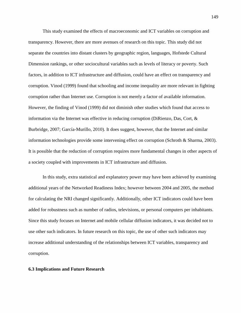
149
14
This study examined the effects of macroeconomic and ICT variables on corruption and
transparency. However, there are more avenues of research on this topic. This study did not
separate the countries into distant clusters by geographic region, languages, Hofstede Cultural
Dimension rankings, or other sociocultural variables such as levels of literacy or poverty. Such
factors, in addition to ICT infrastructure and diffusion, could have an effect on transparency and
corruption. Vinod (1999) found that schooling and income inequality are more relevant in fighting
corruption rather than Internet use. Corruption is not merely a factor of available information.
However, the finding of Vinod (1999) did not diminish other studies which found that access to
information via the Internet was effective in reducing corruption (DiRienzo, Das, Cort, &
Burbridge, 2007; García-Murillo, 2010). It does suggest, however, that the Internet and similar
information technologies provide some intervening effect on corruption (Schroth & Sharma, 2003).
It is possible that the reduction of corruption requires more fundamental changes in other aspects of
a society coupled with improvements in ICT infrastructure and diffusion.
In this study, extra statistical and explanatory power may have been achieved by examining
additional years of the Networked Readiness Index; however between 2004 and 2005, the method
for calculating the NRI changed significantly. Additionally, other ICT indicators could have been
added for robustness such as number of radios, televisions, or personal computers per inhabitants.
Since this study focuses on Internet and mobile cellular diffusion indicators, it was decided not to
use other such indicators. In future research on this topic, the use of other such indicators may
increase additional understanding of the relationships between ICT variables, transparency and
corruption.
6.3 Implications and Future Research

150
15
The results of this study lead to several practical implications. As stated by Vinod (1999),
the Internet’s potential for increasing transparency and reducing corruption is “promising and
obviously vast” (p. 10). Similarly, Soper (2007) found that ICT diffusion, which includes Internet
access, is negatively related to levels of corruption. This study has shown that ICT infrastructure
and diffusion of Internet access does reduce corruption and increase transparency. Government
officials and citizens wishing for more transparency in their governance should campaign for
development in their country’s ICT infrastructure with a focus on providing access to information
via the Internet.
Vinod (1999) put forth that the top five actions in reducing corruption, in order of
importance, are as follows: 1) reducing bureaucratic overhead (e.g. red tape), 2) increasing judiciary
efficiency, 3) increasing GNP per capita, 4), increasing education and economic freedoms, and 5)
reducing inequalities in income. Government officials can use ICTs in the following ways to
achieve some of the actions suggested by Vinod (1999) to promote increases in transparency and
reductions in corruption.
First, the diffusion of ICTs can reduce bureaucratic overhead through such initiatives as e-
governance (Bertot et al., 2010). Specifically, the Internet expands public access to government
information (Cuillier & Piotrowski, 2009; S. M. Johnson, 1998). Secondly, reduced judiciary
efficiency impacts economic growth and infrastructure development by adding additional costs to
private transaction disputes (Buscaglia & Ulen, 1997). One way ICTs can improve judiciary
efficiency is by modernizing (e.g. computerizing) the court case system, thereby giving litigants
better access to the status of their cases (Buscaglia & Ulen, 1997). Diffusion of ICTs coupled with
computerization of the judicial system can also assist attorneys and other legal representatives in
accessing case law and legal opinions of the courts (Shuldberg, 1997).

151
15
Diffusion of ICTs may have some effect on increasing GNP per capita. ICTs have been
found to be a contributing factor in economic growth (Avgerou, 1998). For example, mobile phone
diffusion has been shown to have a positive effect on economic growth and poverty reduction
(Geiger & Mia, 2009). ICTs can not only reduce poverty, but they can also meditate the effects of
poverty by reducing information asymmetry (Sturges, 2004) and improve the quality of life
(Forestier et al., 2002) of the poor. The diffusion of ICTs can also increase education and economic
freedoms by informing citizens of relevant information on government and society. ICTs facilitate
and improve political involvement (Krueger, 2002, 2006; Norris, 2001), and they foster civil and
political freedoms (Baliamoune-Lutz, 2003). Access to ICTs allows citizens to become lifelong
learners who can acquire new skills to meet the demands of changing economic markets (Noe &
Peacock, 2002).
Additionally, Kiiski and Pohjola (2002) found that, in OECD countries, GDP per capita and
Internet access cost explained most of the growth in computer hosts per capita. Beilock and
Dimitrova (2003) also found that Internet usage rates were significantly determined by per capita
income. Future studies should explain GDP per capita as an independent variable effecting the NRI
and Internet and mobile diffusion.
In this study, mobile cellular diffusion did find a negligible negative effect on corruption
and a moderate positive effect on transparency. However, Akpan-Obong et al. (2010) and Bailard
(2009) found that mobile communication technologies significantly accounted for political
development in Africa. Future research should use geographical region as a control variable.
6.4 Conclusion

152
15
The findings presented in this study are mostly consistent with those of other scholars on the
effects of ICTs on improving transparency and governance. (Avgerou, 1998; Krueger, 2002;
Opoku-Mensah, 2000; Soper, 2007). There is no doubt that corruption and transparency need to be
addressed worldwide. As countries and their citizens rapidly adopt ICTs, there is hope that
corruption will be exposed and eradicated through the increased transparency brought about by
access to information. Increased transparency offers the promise of participatory governance, and
technology is one avenue in fulfilling this promise. The results of this study should be taken as a
positive message that ICT diffusion and adoption can decrease corruption and increase transparency
as citizens have access to more information via the Internet.

153
15
REFERENCES
Acemoglu, D., & Verdier, T. (2001). Property rights, corruption and the allocation of talent: A
general equilibrium approach. The Economic Journal, 108(450), 1381-1403. doi:
10.1111/1468-0297.00347
Addison, T., & Heshmati, A. (2004). The new global determinants of FDI flows to developing
countries: The importance of ICT and democratization. In M. Bagella, L. Becchetti, I. Hasan
& W. C. Hunter (Eds.), Monetary Integration: Markets and Regulation (Vol. 4, pp. 151-
186). Oxford, UK: Emerald Group.
Ades, A., & Di Tella, R. (1996). The causes and consequences of corruption: A review of recent
empirical contributions. IDS Bulletin, 27(2), 6-11. doi: 10.1111/j.1759-
5436.1996.mp27002002.x
Ades, A., & Di Tella, R. (1999). Rents, competition, and corruption. The American Economic
Review, 89(4), 982-993.
Aghion, P., & Schankerman, M. (1999). Competition, entry and the social returns to infrastructure
in transition economies. Economics of Transition, 7(1), 79-101. doi: 10.1111/1468-
0351.00005
Agrawal, P. (2003). Economic impact of foreign direct investment in South Asia. In A. Mattoo &
R. M. Stern (Eds.), India and the WTO (pp. 117-140). Washington, DC: World Bank and
Oxford University Press.
Akçay, S. (2006). Corruption and human development. Cato Journal, 26(1), 29-48.
Akerlof, G. A., & Yellen, J. L. (1990). The fair wage-effort hypothesis and unemployment. The
Quarterly Journal of Economics, 105(2), 255-283.

154
15
Akpan-Obong, P., Alozie, N. O., & Foster, W. (2010). Cell vs. Internet: The impact on
democratization in Africa. Paper presented at the 39th Research Conference on
Communication Information and Internet Policy, Arlington, VA.
Alam, M. S. (1995). A theory of limits on corruption and some applications. Kyklos, 483(3), 419-
435.
Allison, P. D. (2001). Missing data. Thousand Oaks, CA: Sage Publications.
Allison, P. D. (2003). Missing data techniques for structural equation modeling. Journal of
Abnormal Psychology, 112(4), 545-557. doi: 10.1037/0021-843X.112.4.545
Amundsen, I. (1999). Political corruption: An introduction to the issues. Bergen, Norway: Chr.
Michelsen Institute.
Andersen, K. N., Henriksen, H. Z., Medaglia, R., Danziger, J. N., Sannarnes, M. K., & Enemærke,
M. (2010). Fads and facts of E-government: A review of impacts of E-government (2003–
2009). International Journal of Public Administration, 33(11), 564-579. doi:
10.1080/01900692.2010.517724
Anderson, J. C., & Gerbing, D. W. (1988). Structural equation modeling in practice: A review and
recommended two-step approach. Psychological Bulletin, 103(3), 411-423.
Andrea, M., & Antonio, M. (2007). The transparency of politics and the quality of politicians.
American Economic Review, 97(2), 311-315.
Andvig, J. C. (1995). Corruption in the North Sea oil industry: Issues and assessments. Crime, Law
and Social Change, 23(4), 289-313.
Andvig, J. C., Fjeldstad, O.-H., Amundsen, I., Sissener, T. K., & Søreide, T. (2000). Research on
corruption: A policy oriented survey. Bergen, Norway: Chr. Michelsen Institute.

155
15
Archibold, R. C. (2012, June 23). Killings curb reporting of Mexican crime wave, The New York
Times, p. A1. Retrieved from http://www.nytimes.com/2012/06/23/world/americas/killings-
curb-reporting-of-mexican-crime-wave.html?pagewanted=all
Arvas, M. A., & Ata, A. Y. (2011). Determinants of economic corruption: A cross-country data
analysis. International Journal of Business & Social Science, 2(13), 161-169.
Avgerou, C. (1998). How can IT enable economic growth in developing countries? Information
Technology for Development, 8(1), 15-28.
Backus, D. K., Kehoe, P. J., & Kydland, F. E. (1994). Dynamics of the trade balance and the terms
of trade: The J-curve? The American Economic Review, 84(1), 84-103.
Backus, M. (2001). E-governance and developing countries: Introduction and examples. The
Hague, Netherlands: International Institute for Communication and Development (IICD).
Bailard, C. S. (2009). Mobile phone diffusion and corruption in Africa. Political Communication,
26(3), 333-353. doi: 10.1080/10584600903053684
Baliamoune-Lutz, M. (2003). An analysis of the determinants and effects of ICT diffusion in
developing countries. Information Technology for Development, 10(3), 151-169.
Barclay, D., Higgins, C., & Thompson, R. (1995). The partial least squares (PLS) approach to
causal modeling: Personal computer adoption and use as an illustration. Technology Studies,
2(2), 285-309.
Bardhan, P. (1997). Corruption and development: A review of issues. Journal of Economic
Literature, 35(3), 1320-1346.
Bates, R. H. (1981). Markets and states in tropical Africa: The political basis of agricultural
policies. Berkeley, CA: University of California Press.

156
15
Baumgartner, H., & Homburg, C. (1996). Applications of structural equation modeling in
marketing and consumer research: A review. International Journal of Research in
Marketing, 13(2), 139-162.
Becker, G. S. (1968). Crime and punishment: An economic approach. The Journal of Political
Economy, 76(2), 169-217.
Becker, G. S., & Stigler, G. J. (1974). Law enforcement, malfeasance, and compensation of
enforcers. Journal of Legal Studies, 3(1), 1-18.
Beilock, R., & Dimitrova, D. V. (2003). An exploratory model of inter-country Internet diffusion.
Telecommunications Policy, 27(3–4), 237-252. doi: 10.1016/s0308-5961(02)00100-3
Bertot, J. C., Jaeger, P. T., & Grimes, J. M. (2010). Using ICTs to create a culture of transparency:
E-government and social media as openness and anti-corruption tools for societies.
Government Information Quarterly, 27(3), 264-271. doi: 10.1016/j.giq.2010.03.001
Billon, M., Marco, R., & Lera-Lopez, F. (2009). Disparities in ICT adoption: A multidimensional
approach to study the cross-country digital divide. Telecommunications Policy, 33(10), 596-
610. doi: http://dx.doi.org/10.1016/j.telpol.2009.08.006
Bland, M. (2002). An introduction to medical statistics. New York, NY: Oxford University Press.
Blomström, M., & Hettne, B. (1984). Development theory in transition: The dependency debate
and beyond: Third world responses. London, UK: Zed Books.
Boretos, G. P. (2007). The future of the mobile phone business. Technological Forecasting and
Social Change, 74(3), 331-340. doi: 10.1016/j.techfore.2005.11.005
Bratton, M., & Van de Walle, N. (1997). Democratic experiments in Africa: Regime transitions in
comparative perspective. Cambridge, UK: Cambridge University Press.
157
15
Brezina, C. (2012). Understanding the gross domestic product and the gross national product. New
York, NY: Rosen Publications.
Briquet, J.-L., & Sawicki, F. (1998). Le clientélisme politique dans les sociétés contemporaines.
Paris, France: Presses Universitaires de France.
Brown, A. J. (2006). What are we trying to measure? Reviewing the basics of corruption definition.
In C. Sampford, A. Shacklock, C. Connors & F. Galtung (Eds.), Measuring Corruption (pp.
57-79). Hampshire, UK: Ashgate.
Brunetti, A., & Weder, B. (2003). A free press is bad news for corruption. Journal of Public
Economics, 87(7-8), 1801-1824. doi: 10.1016/s0047-2727(01)00186-4
Bureau of Economic Analysis. (1991). Gross domestic product as a measure of U.S. production
(Survey of Current Business) (Vol. 71, pp. 8). Washington, DC: United States Department
of Commerce.
Buscaglia, E., & Ulen, T. (1997). A quantitative assessment of the efficiency of the judicial sector
in Latin America. International Review of Law and Economics, 17(2), 275-291. doi:
http://dx.doi.org/10.1016/S0144-8188(97)00007-0
Campos, J. E., Lien, D., & Pradhan, S. (1999). The impact of corruption on investment:
Predictability matters. World Development, 27(6), 1059-1067
Cenfetelli, R. T., & Bassellier, G. (2009). Interpretation of formative measurement in information
systems research. MIS Quarterly, 33(4), 689-707.
Chan, L. S., & Dunn, O. J. (1972). The treatment of missing values in discriminant analysis— 1.
The sampling experiment. Journal of the American Statistical Association, 67(338), 473-
477.

158
15
Chan, L. S., Gilman, J. A., & Dunn, O. J. (1976). Alternative approaches to missing values in
discriminant analysis. Journal of the American Statistical Association, 71(356), 842-844.
Chang, C., Lee, A. C., & Lee, C. F. (2009). Determinants of capital structure choice: A structural
equation modeling approach. The Quarterly Review of Economics and Finance, 49(2), 197-
213. doi: 10.1016/j.qref.2008.03.004
Charoensukmongkol, P., & Moqbel, M. (2012). Does investment in ICT curb or create more
corruption? A cross-country analysis. Public Organization Review, 1-13. doi:
10.1007/s11115-012-0205-8
Cheng, E. W. L. (2001). SEM being more effective than multiple regression in parsimonious model
testing for management development research. The Journal of Management Development,
20(7), 650-667.
Chinn, M. D., & Fairlie, R. W. (2007). The determinants of the global digital divide: A cross-
country analysis of computer and Internet penetration. Oxford Economic Papers, 59(1), 16-
44.
Cho, Y. H., & Choi, B.-D. (2005). E-government to combat corruption: The case of Seoul
metropolitan government. International Journal of Public Administration, 27(10), 719-735.
doi: 10.1081/pad-200029114
Chowdhury, S. K. (2004). The effect of democracy and press freedom on corruption: An empirical
test. Economics Letters, 85(1), 93-101. doi: 10.1016/j.econlet.2004.03.024
Cohen, J. (1988). Statistical power analysis for the behavioral sciences. Hillsdale, NJ: L. Erlbaum
Associates.
159
15
Cohen, R. (1980). The blessed job in Nigeria. In G. M. Britan & R. Cohen (Eds.), Hierarchy and
society: Anthropological perspectives on bureaucracy. Philadelphia, PA: Institute for the
Study of Human Issues, Inc.
Colander, D. C. (1984). Neoclassical political economy: The analysis of rent-seeking and DUP
activities. Cambridge, MA: Ballinger Publishers.
Collins, L. M., Schafer, J. L., & Kam, C. M. (2001). A comparison of inclusive and restrictive
strategies in modern missing data procedures. Psychological Methods, 6(4), 330-351.
Coolidge, J., & Rose-Ackerman, S. (2000). Kleptocracy and reform in African regimes: Theory and
examples. In K. R. Hope & B. C. Chikulo (Eds.), Corruption and development in Africa.
Lessons from country case-studies (pp. 57-86). New York, NY: St. Martin’s Press.
Crenshaw, E. M., & Robison, K. K. (2006). Globalization and the digital divide: The roles of
structural conduciveness and global connection in Internet diffusion. Social Science
Quarterly, 87(1), 190-207.
Crotty, J. (2009). Structural causes of the global financial crisis: A critical assessment of the 'new
financial architecture'. Cambridge Journal of Economics, 33(4), 563-580.
Cuervo-Cazurra, A. (2008). Better the devil you don't know: Types of corruption and FDI in
transition economies. Journal of International Management, 14(1), 12-27. doi:
10.1016/j.intman.2007.02.003
Cuillier, D., & Piotrowski, S. J. (2009). Internet information-seeking and its relation to support for
access to government records. Government Information Quarterly, 26(3), 441-449.
Dasgupta, S., Lall, S., & Wheeler, D. (2001). Policy reform, economic growth, and the digital
divide: An econometric analysis. Washington, DC: World Bank, East Development
Research Group, Infrastructure and Environment.

160
16
De Maria, W. (2008). Measurements and markets: Deconstructing the corruption perception index.
International Journal of Public Sector Management, 21(7), 777-797.
de Mooij, M., & Hofstede, G. (2002). Convergence and divergence in consumer behavior:
Implications for international retailing. Journal of Retailing, 78(1), 61-69. doi:
10.1016/S0022-4359(01)00067-7
de Sardan, J. P. O. (1999). A moral economy of corruption in Africa? Journal of Modern African
Studies, 37(1), 25-52.
Dewan, S., Ganley, D., & Kraemer, K. L. (2005). Across the digital divide: A cross-country multi-
technology analysis of the determinants of IT penetration. Journal of the Association for
Information Systems, 6(12), 409-431.
DiRienzo, C. E., Das, J., Cort, K. T., & Burbridge, J. (2007). Corruption and the role of
information. Journal of International Business Studies, 38(2), 320-332.
Doane, D. P., & Seward, L. E. (2011). Measuring skewness: A forgotten statistic? Journal of
Statistics Education, 19(2), 1-18.
Dodeen, H. M. (2003). Effectiveness of valid mean substitution in treating missing data in attitude
assessment. Assessment & Evaluation in Higher Education, 28(5), 505-513. doi:
10.1080/02602930301674
Dodge, Y., & Marriott, F. H. C. (2003). The Oxford dictionary of statistical terms. New York, NY:
Oxford University Press.
Doig, A., & Theobald, R. (1999). Corruption and democratisation. London, UK: Frank Cass and
Company Limited.
Donchev, D. D., & Ujhelyi, G. (2009). What do corruption indices measure? Retrieved from Social
Science Research Network website: http://ssrn.com/paper=1124066
161
16
Douglass, D. H., Clader, B. D., Christy, J. R., Michaels, P. J., & Belsley, D. A. (2003). Test for
harmful collinearity among predictor variables used in modeling global temperature.
Climate Research, 24, 15-18.
Dunning, T., & Freedman, D. A. (2007). Modeling selection effects. In W. Outhwaite & S. Turner
(Eds.), Handbook of social science methodology (pp. 225-231). London, UK: Sage.
Dutta, S., Lanvin, B., & Paua, F. (2003). The global information technology report 2002-2003:
Readiness for the networked world. New York, NY: Oxford University Press.
Duyne, P. C. (1996). Organized crime, corruption and power. Crime, Law and Social Change,
26(3), 201-238. doi: 10.1007/bf00230862
Easterlin, R. A. (2000). The worldwide standard of living since 1800. The Journal of Economic
Perspectives, 14(1), 7-26.
Enders, C. K., & Bandalos, D. L. (2001). The relative performance of full information maximum
likelihood estimation for missing data in structural equation models. Structural Equation
Modeling: A Multidisciplinary Journal, 8(3), 430-457. doi: 10.1207/S15328007SEM0803_5
Erumban, A. A., & de Jong, S. B. (2006). Cross-country differences in ICT adoption: A
consequence of culture? Journal of World Business, 41(4), 302-314.
Eskeland, G. S., Thiele, H., & World Bank. (1999). Corruption under moral hazard. Washington,
DC: World Bank, Development Research Group, Public Economics.
Farrales, M. J. (2005). What is corruption? A history of corruption studies and the great definitions
debate. Retrieved from Social Science Research Network website:
http://ssrn.com/abstract=1739962
Farrar, D. E., & Glauber, R. R. (1967). Multicollinearity in regression analysis: The problem
revisited. The Review of Economics and Statistics, 49(1), 92-107.

162
16
Forestier, E., Grace, J., & Kenny, C. (2002). Can information and communication technologies be
pro-poor? Telecommunications Policy, 26(11), 623-646.
Friedrich, C. J. (1989). Corruption concepts in historical perspective. In A. J. Heidenheimer, M.
Johnston & V. T. Le Vine (Eds.), Political corruption: A handbook (pp. 15-24). New
Brunswick, Canada: Transaction Publishers.
Galtung, F. (1998). Criteria for sustainable corruption control. European Journal of Development
Research, 10(1), 105-128.
Galtung, F., & Pope, J. (1999). The global coalition against corruption: Evaluating transparency
international. In A. Schedler, L. Diamond & M. F. Plattner (Eds.), The self-restraining state:
Power and accountability in new democracies (pp. 257-282). Boulder, CO: Lynne Rienner.
García-Murillo, M. (2010). The effect of Internet access on government corruption. Electronic
Government: An International Journal, 7(1), 22-40.
Gascó-Hernández, M., Equiza-López, F., & Acevedo-Ruiz, M. (2007). Information communication
technologies and human development: Opportunities and challenges. Hershey, PA: Idea
Group.
Gefen, D. (2000). Structural equation modeling and regression: Guidelines for research practice.
Communications of the Association for Information Systems, 7(7), 1-78.
Geiger, T., & Mia, I. (2009). Mobile telephony: A critical enabler of networked readiness? In S.
Dutta & I. Mia (Eds.), The Global Information Technology Report 2008-2009: Mobility in a
Networked World (pp. 27-35). Geneva, Switzerland: World Economic Forum.
Geisser, S. (1974). A predictive approach to the random effect model. Biometrika, 61(1), 101-107.
doi: 10.2307/2334290
163
16
Getz, K. A., & Volkema, R. J. (2001). Culture, perceived corruption, and economics: A model of
predictors and outcomes. Business & Society, 40(1), 7-30. doi:
10.1177/000765030104000103
Gholami, R., Lee, S. Y. T., & Heshmati, A. (2006). The causal relationship between information
and communication technology and foreign direct investment. World Economy, 29(1), 43-
62. doi: 10.1111/j.1467-9701.2006.00757.x
Girling, J. L. S. (2002). Corruption, capitalism and democracy. London, UK: Routledge.
Goel, R. K., & Nelson, M. A. (1998). Corruption and government size: A disaggregated analysis.
Public Choice, 97(1), 107-120.
Graham, M. H. (2003). Confronting multicollinearity in ecological multiple regression. Ecology,
84(11), 2809-2815.
Gray, C., & Kaufmann, D. (1998). Corruption and development. Finance & Development, 35(1), 7-
10.
Gruber, H., & Verboven, F. (2001). The diffusion of mobile telecommunications services in the
European Union. European Economic Review, 45(3), 577-588. doi: 10.1016/s0014-
2921(00)00068-4
Guillén, M. F., & Suárez, S. L. (2005). Explaining the global digital divide: Economic, political and
sociological drivers of cross-national Internet use. Social Forces, 84(2), 681-708.
Gyimah-Brempong, K. (2002). Corruption, economic growth, and income inequality in Africa.
Economics of Governance, 3(3), 183-209. doi: 10.1007/s101010200045
Habib, M., & Zurawicki, L. (2002). Corruption and foreign direct investment. Journal of
International Business Studies, 33(2), 291-307.

164
16
Haddon, L. (2004). Information and communication technologies in everyday life: A concise
introduction and research guide. Oxford, UK: Berg.
Hair, J. F., Anderson, R. E., & Tatham, R. L. (1987). Multivariate data analysis with readings (2nd
ed.). New York, NY: Macmillan.
Hair, J. F., Black, W. C., Babin, B. J., & Anderson, R. E. (2010). Multivariate data analysis: A
global perspective (7th ed.). Upper Saddle River, NJ: Pearson Education.
Hamilton, D. (1987). Sometimes R2 > r
2yx1 + r
2yx2: Correlated variables are not always redundant.
American Statistician, 41(2), 129-132.
Harriss-White, B., & White, G. (1996). Liberalization and the new corruption. IDS Bulletin, 27(2),
31-39.
Hatcher, L. (1994). A step-by-step approach to using the SAS system for factor analysis and
structural equation modeling. Cary, NC: SAS Institute.
Hawthorne, G., & Elliott, P. (2005). Imputing cross-sectional missing data: Comparison of common
techniques. Australian & New Zealand Journal of Psychiatry, 39(7), 583-590.
Hay, J. R., & Shleifer, A. (1998). Private enforcement of public laws: A theory of legal reform.
American Economic Review, 88(2), 398-403.
Heidenheimer, A. J. (1970). Political corruption: Readings in comparative analysis. New York,
NY: Holt Rinehart and Winston.
Heidenheimer, A. J., Johnston, M., & Le Vine, V. T. (1989). Political corruption: A handbook.
New Brunswick, Canada: Transaction.
Heitjan, D. F., & Basu, S. (1996). Distinguishing "missing at random" and "missing completely at
random". The American Statistician, 50(3), 207-213.

165
16
Hill, K. A., & Hughes, J. E. (1998). Cyberpolitics: Citizen activism in the age of the Internet. Blue
Ridge Summit, PA: Rowman & Littlefield.
Hinkley, D. V. (1977). Jackknifing in unbalanced situations. Technometrics, 19(3), 285-292.
Hofheinz, A. (2005). The Internet in the Arab world: Playground for political liberalization.
International Politics and Society, 2005(3), 78-96.
Hofstede, G. H. (1984). Culture's consequences: International differences in work-related values
(Vol. 5). London, UK: Sage.
Hofstede, G. H. (1997). Cultures and organizations: Software of the mind. New York, NY:
McGraw-Hill.
Hofstede, G. H. (2001). Culture's consequences: Comparing values, behaviors, institutions, and
organizations across nations (2 ed.). Thousand Oaks, CA: Sage Publications.
Hofstede, G. H., Hofstede, G. J., & Minkov, M. (2010). Cultures and organizations (3 ed.).
Chicago, IL: McGraw-Hill.
Honaker, J., & King, G. (2010). What to do about missing values in time-series cross-section data.
American Journal of Political Science, 54(2), 561-581.
Hope, K. R., & Chikulo, B. C. (2000). Corruption and development in Africa: Lessons from country
case-studies. New York, NY: Palgrave.
Hoque, S. M. S. (2005). E-governance in Bangladesh: A scrutiny from the citizens’ perspective. In
R. Ahmad (Ed.), The role of public administration in building a harmonious society (pp.
346-365). Beijing, China: Asian Development Bank, Network of Asia-Pacific Schools and
Institutes of Public Administration and Governance.
Huntington, S. P. (1968a). Modernization and corruption. In S. P. Huntington (Ed.), Political order
in changing societies (pp. 59–71). New Haven, CT: Yale University Press.
166
16
Huntington, S. P. (1968b). Political order in changing societies. New Haven, CT: Yale University
Press.
Husted, B. W. (1999). Wealth, culture, and corruption. Journal of International Business Studies,
30(2), 339-359.
ITU. (2011). ICT services getting more affordable worldwide [Press Release]. Retrieved from
http://www.itu.int/net/pressoffice/press_releases/2011/15.aspx#.UMmCYnfheSo
Jakopin, N. M., & Klein, A. (2011). Determinants of broadband Internet access take-up: Country
level drivers. The Journal of Policy, Regulation and Strategy for Telecommunications,
Information and Media, 13(5), 29-47.
Johnson, S., Kaufmann, D., & Zoido-Lobatón, P. (1998). Regulatory discretion and the unofficial
economy. American Economic Review, 88(2), 387-392.
Johnson, S. M. (1998). The Internet changes everything: Revolutionizing public participation and
access to government information through the Internet. Administrative Law Review, 50(2),
277-282.
Johnston, M. (1997). What can be done about entrenched corruption? Paper presented at the Ninth
Annual Bank Conference on Development Economics, Washington, DC.
Jovanovic, B., & Rob, R. (1989). The growth and diffusion of knowledge. The Review of Economic
Studies, 56(4), 569-582.
Katz, J. E., & Lai, C. H. (2009). News blogging in cross-cultural contexts: A report on the struggle
for voice. Knowledge, Technology & Policy, 22(2), 95-107.
Kaufmann, D., Kraay, A., & Mastruzzi, M. (2007). The worldwide governance indicators project:
Answering the critics (World Bank Policy Research Working Paper 4149). Washington,
DC: World Bank.

167
16
Kaufmann, D., Kraay, A., & Mastruzzi, M. (2009). Governance matters VIII: Aggregate and
individual governance indicators, 1996-2008 (World Bank Policy Research Working Paper
4978). Washington, DC: World Bank.
Kaufmann, D., Kraay, A., & Mastruzzi, M. (2010). The worldwide governance indicators:
Methodology and analytical issues. Hague Journal of the Rule of Law, 3(2), 220-246.
Kaufmann, D., & Wei, S.-J. (1999). Does "grease money" speed up the wheels of commerce?
(NBER Working Paper No. 7093). Cambridge, MA: National Bureau of Economic
Research.
Kautalya, & Rangarajan, L. N. (1992). The Arthashastra. New Delhi, India: Penguin Books India.
Kenichi, I. (2004). Internet use via mobile phone in Japan. Telecommunications Policy, 28(1), 43-
58. doi: 10.1016/j.telpol.2003.07.001
Khan, H. A. (1998). Technology, development and democracy: Limits of national innovation
systems in the age of postmodernism. Cheltenham, UK: Edward Elgar.
Kiiski, S., & Pohjola, M. (2002). Cross-country diffusion of the Internet. Information Economics
and Policy, 14(2), 297-310. doi: 10.1016/s0167-6245(01)00071-3
Kim, H.-W., Chan, H. C., & Gupta, S. (2007). Value-based adoption of mobile Internet: An
empirical investigation. Decision Support Systems, 43(1), 111-126. doi:
10.1016/j.dss.2005.05.009
Kim, J.-O., & Curry, J. (1977). The treatment of missing data in multivariate analysis. Sociological
Methods & Research, 6(2), 215-240. doi: 10.1177/004912417700600206
Kimbro, M. B. (2002). A cross-country empirical investigation of corruption and its relationship to
economic, cultural, and monitoring institutions: An examination of the role of accounting

168
16
and financial statements quality. Journal of Accounting, Auditing & Finance, 17(4), 325-
350. doi: 10.1177/0148558x0201700403
King, G., Honaker, J., Joseph, A., & Scheve, K. (1998). List-wise deletion is evil: What to do about
missing data in political science. American Political Science Review, 95, 49-69.
Kline, R. B. (2010). Principles and practice of structural equation modeling (3rd ed.). New York,
NY: The Guilford Press.
Klitgaard, R. E. (1988). Controlling corruption. Berkeley, CA: University of California Press.
Kock, N. (2011a). Using WarpPLS in e-collaboration studies: Descriptive statistics, settings, and
key analysis results. International Journal of e-Collaboration, 7(2), 1-18.
Kock, N. (2011b). Using WarpPLS in e-collaboration studies: Mediating effects, control and second
order variables, and algorithm choices. International Journal of e-Collaboration, 7(3), 1-13.
doi: 10.4018/jec.2011070101
Kock, N. (2012). WarpPLS 3.0 user manual. Laredo, TX: ScriptWarp Systems.
Kock, N., & Lynn, G. S. (2012). Lateral collinearity and misleading results in variance-based SEM:
An illustration and recommendations. Journal of the Association for Information Systems,
13(7), 546-580.
Kolstad, I., & Wiig, A. (2009). Is transparency the key to reducing corruption in resource-rich
countries? World Development, 37(3), 521-532. doi: 10.1016/j.worlddev.2008.07.002
Krueger, B. S. (2002). Assessing the potential of Internet political participation in the United States.
American Politics Research, 30(5), 476-498. doi: 10.1177/1532673x02030005002
Krueger, B. S. (2006). A comparison of conventional and Internet political mobilization. American
Politics Research, 34(6), 759-776. doi: 10.1177/1532673x06290911

169
16
Kshetri, N., & Cheung, M. K. (2002). What factors are driving China's mobile diffusion? Electronic
Markets, 12(1), 22-26. doi: 10.1080/101967802753433236
Kutner, M. H., Nachtsheim, C., & Neter, J. (2004). Applied linear regression models. Boston, MA:
McGraw-Hill/Irwin.
Laffont, J. J. (2003). The principal agent model: The economic theory of incentives. Cheltenham,
UK: Edward Elgar
Lambsdorff, J. G. (1999a). Corruption in comparative perception. In A. K. Jain (Ed.), Economics of
corruption (pp. 81-109). Boston, MA: Springer US.
Lambsdorff, J. G. (1999b). The transparency international corruption perception index 1999 -
framework document. Transparency International. Berlin, Germany. Retrieved from
http://archive.transparency.org/content/download/2908/18010/file/cpi1999_framework.pdf
Lancaster, T., & Montinola, G. (1997). Toward a methodology for the comparative study of
political corruption. Crime, Law and Social Change, 27(3-4), 185-206.
Larraín, B. F., & Tavares, J. (2004). Does foreign direct investment decrease corruption?
Cuadernos de Economía, 41(123), 199-215.
Lauritzen, S. L. (1995). The EM algorithm for graphical association models with missing data.
Computational Statistics & Data Analysis, 19(2), 191–201.
Lee, S.-Y. T., Gholami, R., & Tong, T. Y. (2005). Time series analysis in the assessment of ICT
impact at the aggregate level – lessons and implications for the new economy. Information
& Management, 42(7), 1009-1022. doi: 10.1016/j.im.2004.11.005
Leff, N. H. (1964). Economic development through bureaucratic corruption. The American
Behavioral Scientist, 8(3), 8-14.

170
17
Leon, M. (1984). In defense of modernity: Talcott Parsons and the utilitarian tradition. American
Journal of Sociology, 89(6), 1273-1305.
Lindell, M. K., & Whitney, D. J. (2001). Accounting for common method variance in cross-
sectional research designs. The Journal of Applied Psychology, 86(1), 114-121.
Little, R. J. A. (1988). A test of missing completely at random for multivariate data with missing
values. Journal of the American Statistical Association, 83(404), 1198-1202.
Little, R. J. A., & Rubin, D. B. (1987). Statistical analysis with missing data. New York, NY:
Wiley.
Little, R. J. A., & Rubin, D. B. (2002). Statistical analysis with missing data (2 ed.). New York,
NY: Wiley.
Luo, Y. (2008). The changing Chinese culture and business behavior: The perspective of
intertwinement between guanxi and corruption. International Business Review, 17(2), 188-
193.
MacMullen, R. (1988). Corruption and the decline of Rome. New Haven, CT: Yale University
Press.
Macrae, J. (1982). Underdevelopment and the economics of corruption: A game theory approach.
World Development, 10(8), 677-687. doi: 10.1016/0305-750x(82)90093-6
Maruyama, G. M. (1998). Basics of structural equation modeling. Thousand Oaks, CA: Sage
Publications.
Mauro, P. (1995). Corruption and growth. The Quarterly Journal of Economics, 110(3), 681-712.
McMullan, M. (1961). A theory of corruption based on a consideration of corruption in the public
services and governments of British colonies and ex-colonies in West Africa. The
Sociological Review, 9(2), 181-201.
171
17
Melody, W. H., Mansell, R., & Richards, B. J. (1986). Information and communication
technologies: Social science research and training. London, UK: Economic and Social
Research Council.
Messner, S. F. (1992). Exploring the consequences of erratic data reporting for cross-national
research on homicide. Journal of Quantitative Criminology, 8(2), 155-173. doi:
10.1007/BF01066742
Moghadam, A. H., & Assar, P. (2008). The relationships between national culture and e-adoption:
A case study of Iran. American Journal of Applied Sciences, 5(4), 369-377.
Moody-Stuart, G. (1997). Grand corruption: How business bribes damage developing countries.
Oxford, UK: WorldView.
MSNIndia. (2010). Caught on camera! Goa police seen selling drugs. MSN News. Retrieved April
21, 2010, Retrieved from http://news.in.msn.com/national/article.aspx?cp-
documentid=3674698
Murphy, C. (2007). Are we Rome? The fall of an empire and the fate of America. Boston, MA:
Houghton Mifflin Co.
Myrdal, G. (1970a). The challenge of world poverty: A world anti-poverty program in outline. New
York, NY: Pantheon Books.
Myrdal, G. (1970b). Corruption as a hindrance to modernization in South Asia. In A. J.
Heidenheimer (Ed.), Political corruption: Readings in comparative analysis (Vol. 2, pp.
951–958). New York, NY: Holt Rinehart and Winston.
Neild, R. R. (2002). Public corruption: The dark side of social evolution. London, UK: Anthem.
Nevitt, J., & Hancock, G. R. (2001). Performance of bootstrapping approaches to model test
statistics and parameter standard error estimation in structural equation modeling. Structural

172
17
Equation Modeling: A Multidisciplinary Journal, 8(3), 353-377. doi:
10.1207/s15328007sem0803_2
Nixon, R. B. (1960). Factors related to freedom in national press systems. Journalism & Mass
Communication Quarterly, 37(1), 13-28.
Noe, R. A., & Peacock, M. (2002). Employee training and development. Boston, MA: McGraw-
Hill/Irwin Boston.
Norris, P. (2001). Digital divide: Civic engagement, information poverty, and the Internet
worldwide. Cambridge, UK: Cambridge University Press.
NTV. (2010). Kenya: Corrupt cops caught in the act (video). The Huffington Post. Retrieved April
21, 2010, Retrieved from http://www.huffingtonpost.com/2009/11/02/kenya-corrupt-cops-
caught_n_342140.html
Nye, J. S. (1967). Corruption and political development: A cost-benefit analysis. The American
Political Science Review, 61(2), 417-427.
O'Brien, R. (2007). A caution regarding rules of thumb for variance inflation factors. Quality and
Quantity, 41(5), 673-690.
OECD. (1991). Technology and productivity: The challenge for economic policy. Paris, France:
OECD Publishing.
Olinsky, A., Chen, S., & Harlow, L. (2003). The comparative efficacy of imputation methods for
missing data in structural equation modeling. European Journal of Operational Research,
151(1), 53-79.
Opoku-Mensah, A. (2000). ICTs as tools of democratization: African women speak out. In E. M.
Rathgeber & E. O. Adera (Eds.), Gender and the information revolution in Africa (pp. 187-
213). Ottawa, Canada: International Development Research Centre.

173
17
Osborne, J. W. (2008). Best practices in quantitative methods. Thousand Oaks, CA: Sage
Publications.
Paldam, M. (2004). The big pattern of corruption: Economics, culture and the seesaw dynamics
(Economics Working Paper No. 1999-11). Aarhus, Denmark: University of Aarhus.
Pathak, R. D., & Prasad, R. S. (2005). Role of e-governance in tackling corruption: The Indian
experience. In R. Ahmad (Ed.), The role of public administration in building a harmonious
society (pp. 434-463). Beijing, China: Asian Development Bank, Network of Asia-Pacific
Schools and Institutes of Public Administration and Governance.
Pathak, R. D., Singh, G., Belwal, R., Naz, R., & Smith, R. F. I. (2008). E-governance, corruption
and public service delivery: A comparative study of Fiji and Ethiopia. Journal of
Administration & Governace, 3(1), 65-79.
Pathak, R. D., Singh, G., Belwal, R., & Smith, R. F. I. (2007). E-governance and corruption-
developments and issues in Ethiopia. Public Organization Review, 7(3), 195-208.
Peters, J. G., & Welch, S. (1978). Political corruption in America: A search for definitions and a
theory, or if political corruption is in the mainstream of American politics why is it not in
the mainstream of American politics research? The American Political Science Review,
72(3), 974-984
Pinto, P. M., & Zhu, B. (2008). Fortune or evil? The effects of inward foreign direct investment on
corruption. Paper presented at the 66th Annual National Conference of the Midwest
Political Science Association, Chicago, IL.
Pirannejad, A. (2011). The effect of ICT on political development: A qualitative study of Iran.
Information Development, 27(3), 186-195. doi: 10.1177/0266666911414386

174
17
Qureshi, I., & Compeau, D. (2009). Assessing between-group differences in information systems
research: A comparison of covariance- and component-based SEM. MIS Quarterly, 33(1),
197-214.
Rahman, H. (2007). Information and communication technologies for economic and regional
developments. Hershey, PA: Idea Group Inc.
Rasiah, R. (2006). Information and communication technology and GDP per capita. International
Journal of Internet and Enterprise Management, 4(3), 202-214.
Rauch, J. E., & Peter, B. E. (2000). Bureaucratic structure and bureaucratic performance in less
developed countries. Journal of Public Economics, 75(1), 49-71.
Raymond, M. R., & Roberts, D. M. (1987). A comparison of methods for treating incomplete data
in selection research. Educational and Psychological Measurement, 47(1), 13-26.
Reilly, M. (1993). Data analysis using hot deck multiple imputation. The Statistician, 42(3), 307-
313.
Reinikka, R., & Svensson, J. (2005). Fighting corruption to improve schooling: Evidence from a
newspaper campaign in Uganda. Journal of the European Economic Association, 3(2/3),
259-267.
Rencher, A. C. (1998). Multivariate statistical inference and applications. New York, NY: Wiley &
Sons.
Ringen, S. (1991). Households, standard of living, and inequality. Review of Income and Wealth,
37(1), 1-13.
Robertson, C. J., & Watson, A. (2004). Corruption and change: The impact of foreign direct
investment. Strategic Management Journal, 25(4), 385-396. doi: 10.1002/smj.382

175
17
Robins, J. M. (1997). Non-response models for the analysis of non-monotone non-ignorable
missing data. Statistics in Medicine, 16(1), 21-37.
Rose-Ackerman, S. (1978). Corruption: A study in political economy. New York, NY: Academic
Press.
Rose-Ackerman, S. (1996). Democracy and 'grand' corruption. International Social Science
Journal, 48(3), 365-380.
Rose-Ackerman, S. (1999). Corruption and government: Causes, consequences, and reform. New
York, NY: Cambridge University Press.
Rose-Ackerman, S. (2008). Corruption and government. International Peacekeeping, 15(3), 328-
343.
Rose, A. K., & Yellen, J. L. (1989). Is there a J-curve? Journal of Monetary Economics, 24(1), 53-
68.
Rosenberg, A. (1992). Economics: Mathematical politics or science of disminishing returns?
Chicago, IL: University of Chicago Press.
Rosenberg, N. (1972). Factors affecting the diffusion of technology. Explorations in Economic
History, 10(1), 3-33.
Rosenthal, R., & Rosnow, R. L. (1991). Essentials of behavioral research: Methods and data
analysis. New York, NY: McGraw-Hill.
Roth, P. L. (1994). Missing data: A conceptual review for applied psychologists. Personnel
Psychology, 47(3), 537-560. doi: 10.1111/j.1744-6570.1994.tb01736.x
Sande, I. G. (1983). Hot-deck imputation procedures. In W. G. Madow & I. Ourin (Eds.),
Incomplete data in sample surveys, volume 3, proceedings of the symposium (pp. 334-350).
New York, NY: Academic Press.

176
17
Schafer, J. L., & Graham, J. W. (2002). Missing data: Our view of the state of the art.
Psychological Methods, 7(2), 147-177. doi: 10.1037/1082-989X.7.2.147
Schroth, P. W., & Sharma, P. (2003). Transnational law and technology as potential forces against
corruption in Africa. Management Decision, 41(3), 296-303.
Scott, J. C. (1969). The analysis of corruption in developing nations. Comparative Studies in
Society and History, 11(3), 315-341.
Selden, T. M., & Song, D. (1995). Neoclassical growth, the J curve for abatement, and the inverted
U curve for pollution. Journal of Environmental Economics and Management, 29(2), 162-
168. doi: http://dx.doi.org/10.1006/jeem.1995.1038
Sharma, R. S., Ng, E. W. J., Dharmawirya, M., & Lee, C. K. (2008). Beyond the digital divide: A
conceptual framework for analyzing knowledge societies. Journal of Knowledge
Management, 12(5), 151-164.
Shim, D. C., & Eom, T. H. (2009). Anticorruption effects of information communication and
technology (ICT) and social capital. International Review of Administrative Sciences, 75(1),
99-116.
Shirk, D. A. (2010). Drug violence in Mexico: Data and analysis from 2001-2009. Trends in
Organized Crime, 13(2-3), 167-174.
Shleifer, A., & Vishny, R. W. (1993). Corruption. The Quarterly Journal of Economics, 108(3),
599-617.
Shook, C. L., Ketchen, D. J., Hult, G. T. M., & Kacmar, K. M. (2004). An assessment of the use of
structural equation modeling in strategic management research. Strategic Management
Journal, 25(4), 397-404.

177
17
Shuldberg, K. (1997). Digital influence: Technology and unpublished opinions in the federal courts
of appeals. California Law Review, 85(2), 541-575. doi: 10.2307/3481076
Singh, H., Das, A., & Joseph, D. (2007). Country-level determinants of e-government maturity.
Communications of the Association for Information Systems, 20(1), 632-648.
Smith, A. (1776). The wealth of nations. London, UK: Penguin Books.
Sokal, R. R., & Rohlf, F. J. (1969). Biometry: The principles and practice of statistics in biological
research. San Francisco, CA: W.H. Freeman.
Soper, D. S. (2007). ICT investment impacts on future levels of democracy, corruption, and e-
government acceptance in emerging countries. Paper presented at the 13th Americas
Conference on Information Systems (AMCIS), Keystone, CO.
Soper, D. S., & Demirkan, H. (2012). How ICTs affect democracy and corruption in emerging
societies. IEEE IT Professional, 14(4), 18-23. doi: 10.1109/MITP.2012.51
Steenkamp, J. B., & Baumgartner, H. (2000). On the use of structural equation models for
marketing modeling. International Journal of Research in Marketing, 17(2-3), 195-202.
Stiglitz, J. E. (2009). GDP fetishism. The Economists' Voice, 6(8), 5. doi: 10.2202/1553-3832.1651
Stinger, C. L. (1985). The renaissance in Rome. Bloomington, IL: Indiana University Press.
Stone, M. (1974). Cross-validatory choice and assessment of statistical predictions. Journal of the
Royal Statistical Society. Series B (Methodological), 36(2), 111-147. doi: 10.2307/2984809
Straub, D., Keil, M., & Brenner, W. (1997). Testing the technology acceptance model across
cultures: A three country study. Information & Management, 33(1), 1-11. doi:
10.1016/S0378-7206(97)00026-8
Stulz, R. M., & Williamson, R. (2003). Culture, openness, and finance. Journal of Financial
Economics, 70(3), 313-349.

178
17
Sturges, P. (2004). Corruption, transparency and a role for ICT? International Journal of
Information Ethics, 2(11), 1-9.
Suh, T., & Khan, O. J. (2003). The effect of FDI inflows and ICT infrastructure on exporting in
ASEAN/AFTA countries: A comparison with other regional blocs in emerging markets.
International Marketing Review, 20(5), 554-571.
Svensson, J. (2005). Eight questions about corruption. Journal of Economic Perspectives, 19(3), 19-
42.
Tabachnick, B. G., & Fidell, L. S. (1996). Using multivariate statistics. New York, NY:
HarperCollins.
Tanzi, V. (1995). Corruption, governmental activities, and markets. Finance & Development, 32,
24-27.
Titman, S., & Wessels, R. (1988). The determinants of capital structure choice. The Journal of
Finance, 43(1), 1-19.
Treisman, D. (2000). The causes of corruption: A cross-national study. Journal of Public
Economics, 76(3), 399–457. doi: 10.1016/S0047-2727(99)00092-4
United Nations. (1999). Global report on crime and justice. New York, NY: The United Nations
Office for Drug Control and Crime Prevention.
United Nations. (2000). The world's women 2000: Trends and statistics. New York, NY: United
Nations Statistical Division.
United Nations. (2012). Member states of the United Nations. Retrieved April 14, 2012, 2012,
Retrieved from http://www.un.org/en/members/index.shtml

179
17
Vinod, H. D. (1999). Statistical analysis of corruption data and using the Internet to reduce
corruption. Journal of Asian Economics, 10(4), 591-603. doi: 10.1016/s1049-
0078(00)00034-8
Waheeduzzaman, A. N. M. (2005). Tripolar world of corruption and inequality: Again, the
difference is in freedom and governance. Journal of Transnational Management
Development, 9(4), 37-48.
Wallsten, S. (2005). Regulation and Internet use in developing countries. Economic Development
and Cultural Change, 53(2), 501-523.
Wang, M., & Fitzmaurice, G. M. (2006). A simple imputation method for longitudinal studies with
non-ignorable non-responses. Biometrical Journal, 48(2), 302-318. doi:
10.1002/bimj.200510188
Warf, B. (2001). Segueways into cyberspace: Multiple geographies of the digital divide.
Environment and Planning B: Planning and Design, 28(1), 3-19.
Warschauer, M. (2002). Reconceptualizing the digital divide. First Monday. Retrieved from
http://firstmonday.org/htbin/cgiwrap/bin/ojs/index.php/fm/article/view/967/888
Weber, M. (1958). The three types of legitimate rule. Berkeley Publications in Society and
Institutions, 4(1), 1-11.
Wei, S.-J. (1997). Why is corruption so much more taxing than tax? Arbitrariness kills (NBER
Working Paper No 6255). Cambridge, MA: National Bureau of Economic Research.
Wei, S.-J. (2000). How taxing is corruption on international investors? The Review of Economics
and Statistics, 82(1), 1-11.
Wilson, R. C. (1989). Ancient republicanism: Its struggle for liberty against corruption. New York,
NY: Peter Lang.

180
18
Wright, S. (1934). The method of path coefficients. The Annals of Mathematical Statistics, 5(3),
161-215. doi: 10.1214/aoms/1177732676
Zar, J. H. (1999). Biostatistical analysis. Upper Saddle River, NJ: Prentice Hall.
181
18
VITA
Leebrian E. Gaskins
PROFESSIONAL EXPERIENCE
Associate Vice President of Information Technology/Chief Information Officer February 2005 to Present
Associate Director of Computer and Telecommunications Services October 2002 to Present
Texas A&M International University, Laredo, TX
Information Systems Specialist, Local Area Networking Specialist July 1997 to October 2002
West Virginia University, Health Science Center
Information Systems Assistant August 1996 to January 1997
West Virginia University, Housing and Residence Life
Network Manager Assistant August 1992 to December 1995
West Virginia University, College of Business & Economics
EDUCATION
Doctor of Philosophy in International Business Administration
Concentration: Management of Information System
Texas A&M International University, Laredo, TX, 2013
Master of Business Administration
Concentration: Information System
West Virginia University, Morgantown, WV, 2002
Master of Arts in Technology Education
Concentration: Communication and Information Systems
West Virginia University, Morgantown, WV, 2000
Bachelor of Arts in Psychology
West Virginia University, Morgantown, WV, 1996
RESEARCH PRESENTATIONS AND PUBLICATIONS
Gaskins, L., Ujah, N., & Ortiz, J. (2011). When 1st and 3rd converge: A border region framework. Journal of Diversity
Management, 6(1), 11-20.
Sagafi-nejad, T., Smith, L.M., Byrne, S., Gaskins, L., Nguyen, Z., & Sexton, S. (2010, March). Moving toward
International Financial Reporting Standards (IFRS) in North America. Paper presented at the American
Accounting Association Southwest Region annual meeting, Dallas, Texas.
Sagafi-nejad, T., Smith, L.M., Byrne, S., Gaskins, L., Nguyen, Z., & Sexton, S. (2010). Moving toward International
Financial Reporting Standards (IFRS) in North America. Internal Auditing, 25(1), 3-9.