the effect of job displacement on the transitions to ...ftp.iza.org/dp3069.pdfthe effect of job...

IZA DP No. 3069

The Effect of Job Displacement on the Transitionsto Employment and Early Retirement for OlderWorkers in Four European Countries

Konstantinos Tatsiramos

DI

SC

US

SI

ON

PA

PE

R S

ER

IE

S

Forschungsinstitutzur Zukunft der ArbeitInstitute for the Studyof Labor

September 2007

The Effect of Job Displacement on the Transitions to Employment and Early

Retirement for Older Workers in Four European Countries

Konstantinos Tatsiramos IZA

Discussion Paper No. 3069 September 2007

IZA

P.O. Box 7240 53072 Bonn

Germany

Phone: +49-228-3894-0 Fax: +49-228-3894-180

E-mail: [email protected]

Any opinions expressed here are those of the author(s) and not those of the institute. Research disseminated by IZA may include views on policy, but the institute itself takes no institutional policy positions. The Institute for the Study of Labor (IZA) in Bonn is a local and virtual international research center and a place of communication between science, politics and business. IZA is an independent nonprofit company supported by Deutsche Post World Net. The center is associated with the University of Bonn and offers a stimulating research environment through its research networks, research support, and visitors and doctoral programs. IZA engages in (i) original and internationally competitive research in all fields of labor economics, (ii) development of policy concepts, and (iii) dissemination of research results and concepts to the interested public. IZA Discussion Papers often represent preliminary work and are circulated to encourage discussion. Citation of such a paper should account for its provisional character. A revised version may be available directly from the author.

mailto:[email protected]

IZA Discussion Paper No. 3069 September 2007

ABSTRACT

The Effect of Job Displacement on the Transitions to Employment and Early Retirement for Older Workers

in Four European Countries*

Despite the increased frequency of job loss for older workers in Europe, little is known on its effect on the work-retirement decision. Employing individual data from the European Community Household Panel for Germany, Italy, Spain, and the U.K., a multivariate competing-risks hazard model is estimated in which the effect of job displacement is identified separately for transitions into re-employment and retirement. The findings suggest that in countries with institutional provisions for older unemployed which offer a pathway to early retirement such as, Germany and Spain, older displaced workers exhibit lower re-employment and higher retirement rates compared to the non-displaced. These results are robust to dynamic selection due to unobserved heterogeneity and to the endogeneity of displacement. JEL Classification: J14, J26, J63, J64 Keywords: job displacement, job loss, unemployment duration, retirement, competing risks Corresponding author: Konstantinos Tatsiramos IZA P.O. Box 7240 53072 Bonn Germany E-mail: [email protected]

* The financial support provided through the European Community's Human Potential Programme under contract HPRN-CT-2002-00235, [AGE] is greatly acknowledged.

mailto:[email protected]

1. Introduction

This paper investigates the effect of job displacement on the transitions into re-employment, or

retirement, in a competing-risks hazard framework for a number of European countries. In recent

years, there is evidence of an increase in the frequency of job loss among older workers both in the

U.S. (Farber, Haltiwagner, Abraham, 1997; Farber, 2004) and in Europe (OECD, 1998).2 Despite

this development, which has been associated with demand shifts, restructuring of traditional

industries, import competition and out-sourcing of jobs, surprisingly very little is known on how job

displacement might affect the labor market transitions of older workers and, in particular, the work-

retirement decision. Understanding the link between job displacement and retirement has direct

implications for policies promoting longer working lives. These policies are considered as a

response to the decline in the labor force participation of older workers and the demographic

changes that occur in European countries, which put pressure on the sustainability of the social

security systems.

In theory, the direction of the effect of job loss towards re-employment, or retirement, is

ambiguous. Experiencing a job loss may have considerable consequences because of the

interruption of a long tenure job, which diminishes acquired firm-specific human capital,

employment and earning prospects. Indeed, studies focusing on workers of all ages find that job

displacement leads to a reduction of future earnings (Jacobson, LaLonde, Sullivan, 1993; Ruhm,

1991) and an increase of employment instability (Stevens, 1997), in the sense that the displaced

have higher exit rates from subsequent employment.3 Although the unemployment rate among

workers 45 to 64 years old is lower than the overall rate in most OECD countries, the incidence of

long-term unemployment is significantly higher (OECD, 1998), suggesting a lower mobility of

older workers who experience unemployment. Considering retirement as a distinct labor market

2 In what follows job loss and job displacement will be used interchangeably. 3 For a survey on the effect of job displacement see Kletzer (1998). Kuhn (2002) contains an analysis of work displacement for prime age workers for a number of European countries.

2

state allows to distinguish between two competing explanations for the incidence of long-term

unemployment among older workers. That is, unemployment persistence might exist due to 1)

difficulties to be re-employed based on poor employment prospects, or 2) due to disincentives to be

re-employed. The combination of extended unemployment benefit periods with early retirement

schemes available for the older workers, in a number of countries, might affect their decisions by

making retirement more attractive (Duval, 2003).4

However, job displacement might also affect the work-retirement decision on the opposite

direction; reducing wealth and income, which might lead to an extension of the working life.

Focusing on the transitions between non-employment and employment following a late-career job

loss in the U.S., Chan and Stevens (1999, 2001) find that a job loss for men leads to longer labor

force participation reflecting the need to rebuild diminished savings for retirement. For women, the

reduced earnings due to a job loss reduce the incentives to work. Using Austrian administrative

data, Ichino, Schwerdt, Winter-Ebmer, and Zweimüller (2006) find that after a plant closure

initially the old have lower re-employment probabilities as compared to prime-age workers, but

later they catch-up.

The analysis in this paper has three novel and important features. The first is the focus on the

distinction between transitions towards re-employment and retirement for older workers in a

number of countries (Germany, Italy, Spain, and the U.K.), which differ in their institutions related

to older unemployed, based on individual panel data from the European Community Household

Panel (ECHP, 1994-2001). In this respect, the paper contributes to a relatively recent literature on

the incentive effects of unemployment related benefits for older workers. Heyma and Van Ours

(2005) find that the abolition of the requirement to actively search for a job beyond age 57.5 and the

entitlement to unemployment benefits until the age of 65, in the Netherlands, has a large negative

effect on the job finding rate. Other studies have shown that increases in the entitlement period of 4 The literature on retirement has focused on the incentive structure of the pension systems in explaining the observed retirement patterns (e.g. Gruber and Wise, 1998; Meghir and Whitehouse, 1997). Rigidities in the labor market, such as the inability to choose flexible working hours, might also lead to early withdrawal from the labor force even if older workers might prefer to retire gradually (Hurd, 1996).

3

unemployment benefits for older workers leads to declines in transition rates to employment in

Germany (Hunt, 1995) and Austria (Lalive and Zweimüller, 2004), and provide a quantitatively

important pathway into early retirement (Lalive, 2006). Kyyrä and Wilke (2007), evaluating the

increase in the eligibility age from 53 to 55 of the unemployment insurance system in Finland,

which allows unemployed workers to collect benefits up to a certain age limit and then retire, find

evidence of a large decrease in the inflow to unemployment and a large increase in the transition

rate out of unemployment to employment.

The second novel feature of the paper is the joint estimation of the effects of job displacement

on the transitions to and out of subsequent employment, distinguishing between the short and long-

run effects of displacement. That is, although displaced workers might be re-employed relatively

fast, what is important for the overall employment rate is also the stability of the post-displacement

employment. In addition, dynamic selection is taken into account by allowing unobserved

individual characteristics to be correlated across states.

Finally, the paper addresses the endogeneity of displacement by extending the econometric

model into a joint estimation of the selection process into displacement and the transitions into

employment, or retirement. Based on the “timing of the events” approach of Abbring and Van den

Berg (2003), the causal effect of displacement is identified by means of the variation from the

multiple non-employment and employment spells, which are observed for each individual.

The rest of the paper is organized as follows. Section 2 contains a brief discussion of the

institutional features related to unemployment insurance and retirement rules in each of the

countries considered in this study. Section 3 describes the data and provides a non-parametric

analysis of labor market transitions. Section 4 presents the econometric model and discusses

identification and the way to address the endogeneity of displacement. Section 5 provides the

results of the effect of displacement on labor market transitions, and the last section concludes this

paper with a summary of the findings.

4

2. Institutional Features

The focus of this section is on the institutions which are related to older unemployed in the four

countries considered in the analysis. These refer to the unemployment insurance and early

retirement schemes based on information obtained from the Mutual Information System on Social

Protection (MISSOC, 1994) of the European Union.

In Germany, the legal retirement age is 60 after 180 contribution months if unemployed at the

commencement of the pension and if unemployed for 52 weeks after completion of the age of 58.5.

Alternatively, the requirement is to have worked part time for older workers for 24 calendar

months. The age limit for early pension for unemployed increased in the years 1997 to 2001 from

60 to 65 years. However, the pensions can be claimed after the completion of the age of 60 with the

acceptance of pension reductions. The replacement rate for unemployment insurance recipients is

67 per cent of net earnings (60 per cent for beneficiaries without children). The duration of benefits

is 32 months for workers aged 54 and over. In Spain, there is no direct provision of early retirement

for unemployed. However, early retirement is possible at the age of 60 with an 8% reduction for

every anticipated retirement year. With respect to benefits for older unemployed, under the

Industrial Restructuring law, workers are entitled to a form of benefit financed under the relevant

restructuring plan. These benefits are of particular significance for workers aged at least 55 at the

time of restructuring, who may draw them until they reach 65 years of age. The replacement rate for

unemployment insurance recipients is 70 per cent for the first 180 days, and 60 per cent afterwards.

The duration of unemployment benefits received varies between 4 months and 2 years depending on

the contribution period over the preceding 6 years. For long-term unemployed, aged 45 or more,

there is a special 6-months benefit of 75-125 per cent of minimum wage.

In Italy, there are no special benefits for older unemployed which are associated with the

possibility of early retirement. The legal retirement age is 63 for men and 58 for women. Early

pension is available at the age of 54 and after 35 years of contributions, or after 36 years of

contributions regardless of age. Early retirement is possible for employees of companies in

5

economic difficulties at the latest 5 years before normal retirement age. The replacement rate for the

ordinary unemployment benefits is 30% of the average pay received during the last 3 months, and

the duration is 180 days. The replacement rate for the special unemployment benefit for those in the

building industry is 80% of previous earnings with duration of 90 days. In the U.K., there are no

provisions of early retirement and no benefits related to older unemployed. The standard

unemployment insurance rate is a flat rate of about 80 euros per week for aged 25 or over, with

duration up to 12 months limited to 182 days in any job-seeking period in October 1996.

To summarize, in Germany, and Spain, institutions are designed to assist older unemployed

and displaced, while in Italy, and the U.K., such provisions are not in general available. It is worth

mentioning that this does not preclude special schemes with incentives for early retirement, for

instance, in Italy. However, these are case-specific and do not have a general applicability.

3. Data and Descriptive Analysis

The analysis is based on individual data from the European Community Household Panel (ECHP,

1994-2001). The ECHP is a survey based on a standardized questionnaire with annual interviews of

a representative panel of households and individuals from the population in each country, covering

a wide range of topics including demographics, employment characteristics, education etc. In the

first wave, a sample of some 60,500 nationally representative households - approximately 130,000

adults aged 16 years and over - were interviewed in the then 12 Member States. There are three

characteristics that make the ECHP relevant for this study. That is, the simultaneous coverage of

employment status, the standardized methodology and procedures yielding comparable information

across countries and the longitudinal design in which information on the same set of households and

persons is gathered.

The ECHP contains, for every individual in each wave, monthly information on the labor

market status during the previous year distinguishing between unemployment, inactivity,

employment and retirement. An inflow sample of non-employed is constructed from all individuals

6

45 to 64 years old, at the time of the first interview, who respond in at least two consecutive years

of the survey. The inflow sample consists of those who exit employment entering into either

unemployment, or inactivity. Transitions from employment directly to retirement are few in this age

group and are not included in the inflow sample of unemployed and inactive (those who are not

looking for a job but are not retired) denoted as non-employed.

Each non-employment spell can end by either returning into employment, or by retiring.

Missing values of the monthly labor market status are imputed following Blau and Riphahn (1999)

when the missing months are less, or equal to three.5 The analysis allows for multiple non-

employment spells. Table 1 contains statistics of the sample by country.

[Table 1 about here]

The first row shows the total number of individuals, while the second row those who are non-

employed at least once during the sampling period. The inflow sample of individuals used in the

analysis consists of those who have at least one flow into non-employment. These numbers vary

from 379 individuals, for Italy, to 709 for Germany (row 3), while the number of spells varies from

781, for the U.K., to 1801 for Spain (row 4). After dropping those spells with missing information

on displacement, the remaining samples consists of 1064 spells for Germany, 765 for Italy, 1561 for

Spain, and 717 for the U.K.


Table 2 presents the transitions that occur in the sample. Non-employment spells might end

either into employment, or to retirement. The spells for which no transitions out of non-employment

are observed until the end of the sample period are treated as right censored. About 50 per cent of

the non-employment spells in Germany, and 65-68 per cent in Italy, Spain, and the U.K., end by

5 The missing information is replaced with the value of the month before the missing when the values are the same before and after the missing month. With different values, the imputation depends on the number of missing months. Missing information is replaced with the value of the month after the missing month when the missing month is only one. With two missing months, the first missing value is replaced with the value of the previous month and the second missing value is replaced with the value of the next month. With three missing values, the first missing month is replaced with the value of the previous to month, while the other two missing months are replaced with the value of the month after the missing months.

7

returning to employment. The share of spells which end to retirement is about 7 per cent for Italy,

Spain, and the U.K., while it is much higher – about 20 per cent - for Germany. For those being re-

employed, 58 per cent make a transition back to non-employment in Germany, about 75 per cent in

Italy and Spain, and 45 per cent in the U.K.6

For each of the non-employment spells an indicator of displacement is constructed using the

information on the reason for leaving the previous job. The displaced are defined as those who were

obliged to stop the previous job by the employer. Table 3 presents summary statistics of individual

characteristics by displacement status. Older individuals with medium, or low education, are more

likely to be displaced. For the other characteristics, no clear pattern seems to exist across countries.


The advantage of using survey data compared to administrative data is that the sample is more

representative of the whole population of displaced workers. With administrative data displacement

is defined using information on plant closures which excludes all involuntary job separations that

occur on an individual basis. Moreover, with survey data a control group can be defined out of

those who voluntarily left their previous job (for a better job, marriage, child birth, looking after

others, illness, etc.). However, using survey data has the disadvantage of relying on self-reported

information for the reason of job separation, which might be correlated with individual unobserved

characteristics, or be endogenous to labor market institutions. For instance, quits might be reported

as layoffs for the worker to be eligible for unemployment insurance, or layoffs to be reported as

quits to avoid administrative burden on the side of the employer in countries with strict employment

protection legislation. In addition, even in the case of plant closing, the workers who remain until

the plant closes are selected non-randomly from the group of workers who were present when the

6 The paper is focused on Germany, Italy, Spain, and U.K., as for the other countries in the ECHP the inflow sample was relatively small resulting in very few transitions especially towards retirement. As the focus of the paper is on the distinction between transitions to re-employment and retirement this selection was inevitable. However, as discussed in section 2, the four countries studied offer interesting variation in institutional characteristics, representing different welfare regimes.

8

firm’s initial negative demand shocks arrived. This occurs as the firm learns which employees are

likely to quit and alters its layoff policies accordingly (Pfann and Hamermesh, 2001).7

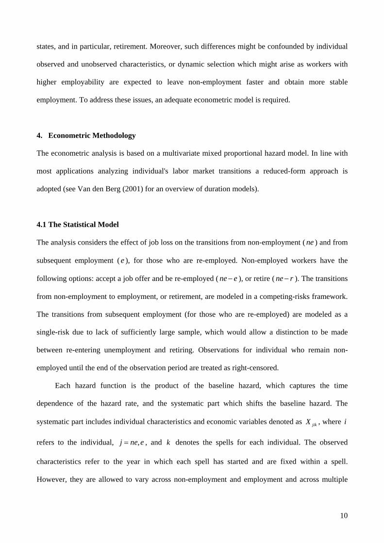
3.1 Empirical Hazard Estimates

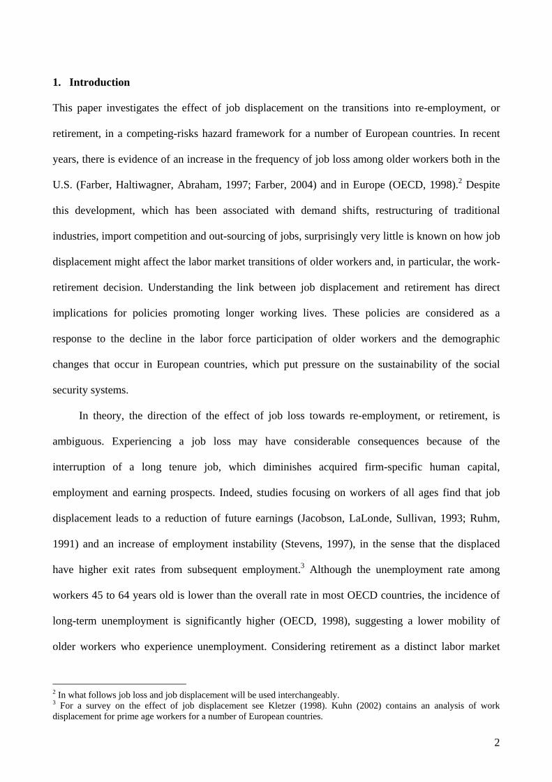
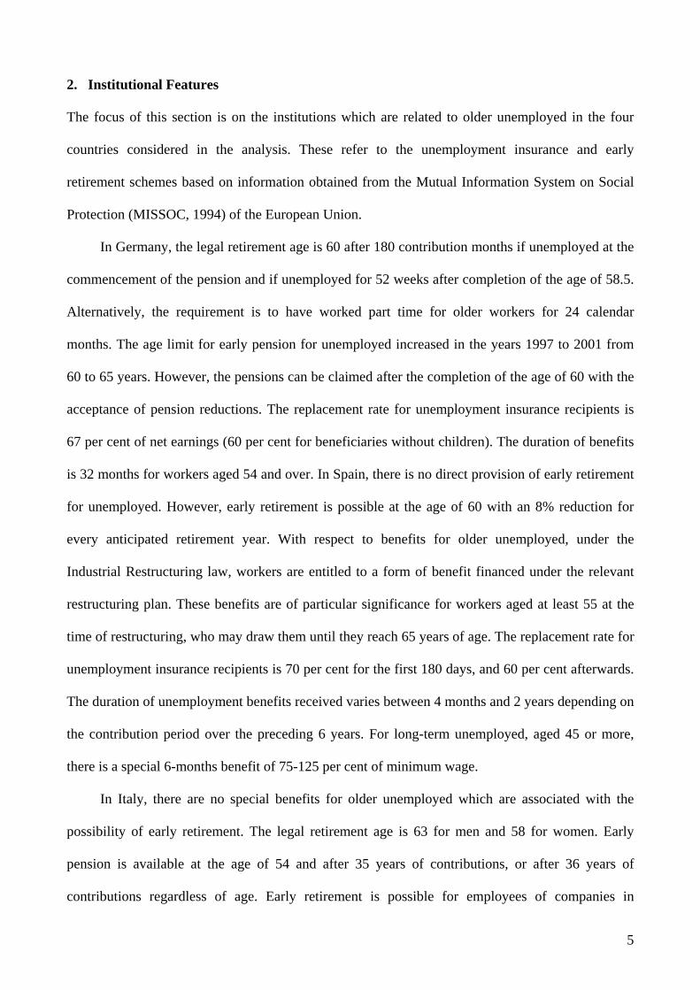
Figure 1 shows the proportion of non-employed who re-enter employment by displacement status.

The cumulative failure is based on the empirical (Kaplan-Meier) hazard rates and is equal to one

minus the survival rate. In Italy and Spain, non-displaced workers return to employment faster

compared to those displaced. The same holds for Germany, although the difference between

displaced and non-displaced appears to be smaller, as is the case for the U.K., but to the opposite

direction.

[Figure 1 about here]

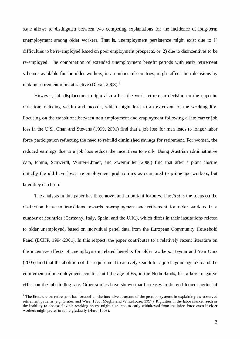
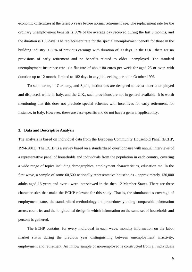
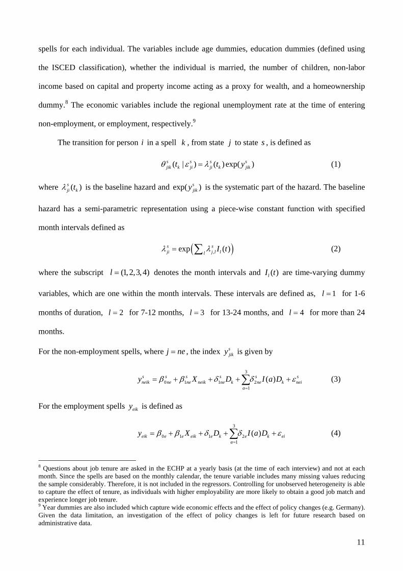
Figure 2 shows the cumulative failure from non-employment to re-employment for the displaced by

age groups. In Germany, and Spain, there is a big difference across age groups in the proportion of

displaced workers who return to employment. While for those aged 45-54 more than 60 per cent

eventually return to employment, it is only about 40 per cent of those older displaced (aged 55-64)

who are re-employed. For Italy and the U.K., such differences by age are smaller. These figures

suggest that, for workers in Germany and Spain, displacement past a certain age (around 55 years

old) is not "repaired".


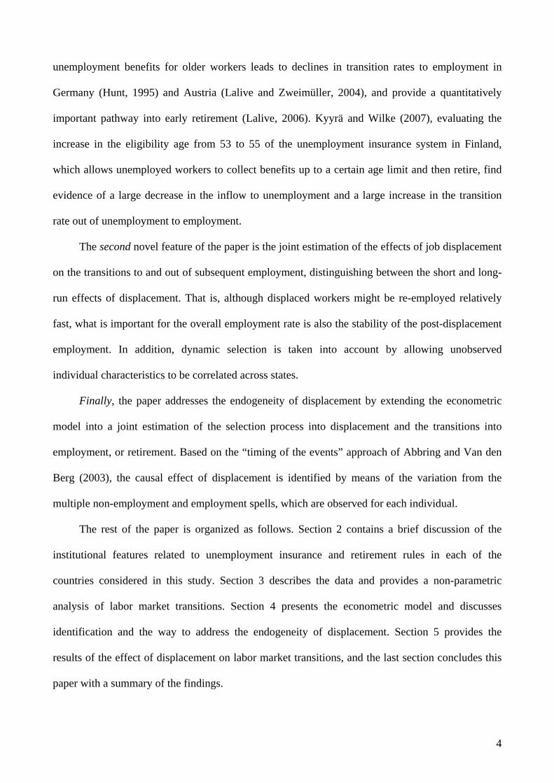
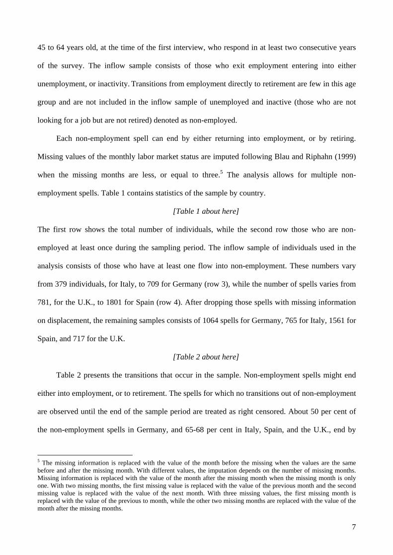
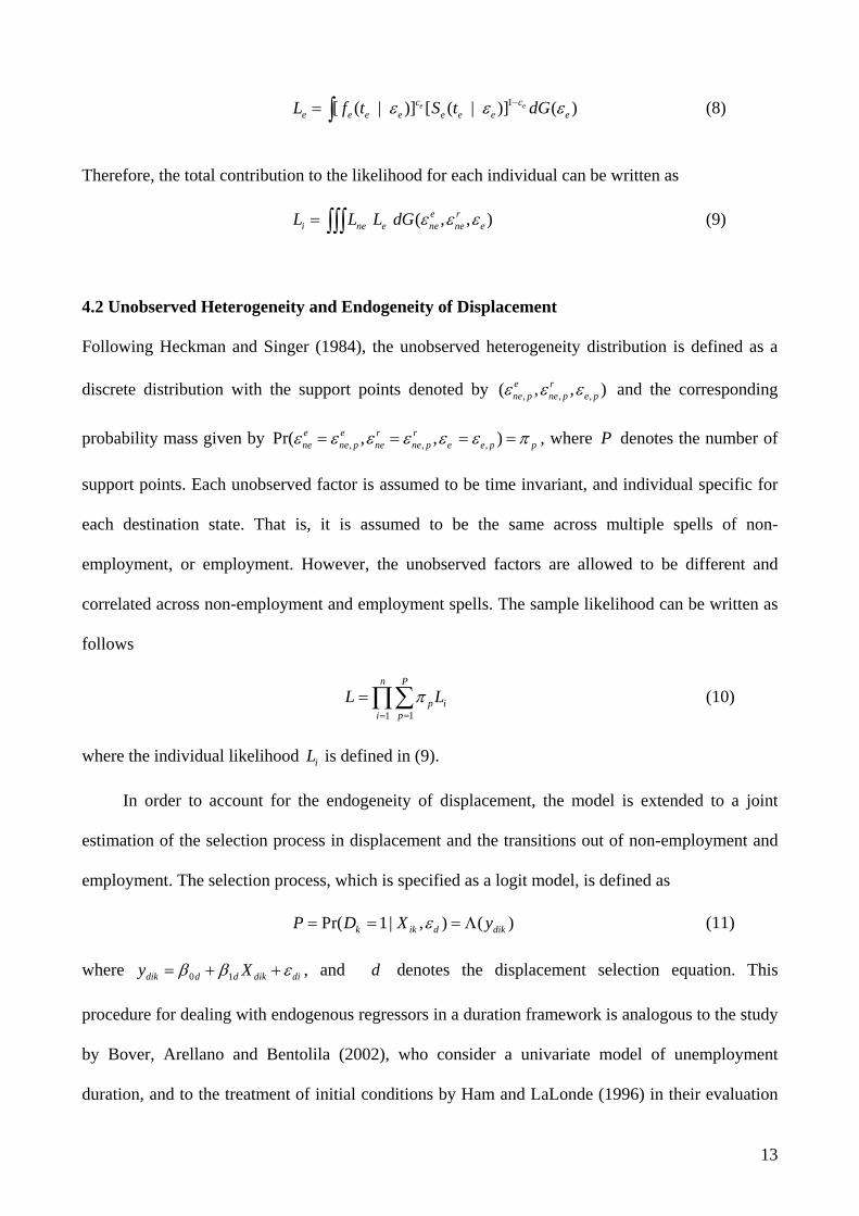
Figure 3 depicts the proportion of workers who exit subsequent employment. It shows that in

countries in which displaced are less likely to return to employment (Italy, Spain) those who do

return exit employment at a lower rate.


Although differences in re-employment and subsequent employment hazards between

displaced and non-displaced are useful, they are not informative on the transitions towards other

7 The way to address the endogeneity of displacement is discussed in Section 4.2.

9

states, and in particular, retirement. Moreover, such differences might be confounded by individual

observed and unobserved characteristics, or dynamic selection which might arise as workers with

higher employability are expected to leave non-employment faster and obtain more stable

employment. To address these issues, an adequate econometric model is required.

4. Econometric Methodology

The econometric analysis is based on a multivariate mixed proportional hazard model. In line with

most applications analyzing individual's labor market transitions a reduced-form approach is

adopted (see Van den Berg (2001) for an overview of duration models).

4.1 The Statistical Model

The analysis considers the effect of job loss on the transitions from non-employment ( ) and from

subsequent employment ( ), for those who are re-employed. Non-employed workers have the

following options: accept a job offer and be re-employed (

ne

e

ne e− ), or retire ( ). The transitions

from non-employment to employment, or retirement, are modeled in a competing-risks framework.

The transitions from subsequent employment (for those who are re-employed) are modeled as a

single-risk due to lack of sufficiently large sample, which would allow a distinction to be made

between re-entering unemployment and retiring. Observations for individual who remain non-

employed until the end of the observation period are treated as right-censored.

ne r−

Each hazard function is the product of the baseline hazard, which captures the time

dependence of the hazard rate, and the systematic part which shifts the baseline hazard. The

systematic part includes individual characteristics and economic variables denoted as jikX , where

refers to the individual, , and denotes the spells for each individual. The observed

characteristics refer to the year in which each spell has started and are fixed within a spell.

However, they are allowed to vary across non-employment and employment and across multiple

i

,j ne e= k

10

spells for each individual. The variables include age dummies, education dummies (defined using

the ISCED classification), whether the individual is married, the number of children, non-labor

income based on capital and property income acting as a proxy for wealth, and a homeownership

dummy.8 The economic variables include the regional unemployment rate at the time of entering

non-employment, or employment, respectively.9

The transition for person i in a spell k , from state to state , is defined as j s

( | ) ( ) exp( )s s s sjik k ji ji k jikt tθ ε λ= y (1)

where is the baseline hazard and is the systematic part of the hazard. The baseline

hazard has a semi-parametric representation using a piece-wise constant function with specified

month intervals defined as

( )sji ktλ exp( )s

jiky

( ),exp ( )s sji j l ll

I tλ λ= ∑ (2)

where the subscript denotes the month intervals and (1,2,3,4)l = ( )lI t are time-varying dummy

variables, which are one within the month intervals. These intervals are defined as, for 1-6

months of duration, for 7-12 months,

1l =

2l = 3l = for 13-24 months, and for more than 24

months.

4l =

For the non-employment spells, where j ne= , the index sjiky is given by

3

0 1 1 21

( )s s s s sneik ne ne neik ne k ne k nei

a

y X D I a D sβ β δ δ=

= + + + +∑ ε (3)

For the employment spells is defined as eiky

3

0 1 1 21

( )eik e e eik e k e k eia

y X D I a Dβ β δ δ=

= + + + +∑ ε

(4)

8 Questions about job tenure are asked in the ECHP at a yearly basis (at the time of each interview) and not at each month. Since the spells are based on the monthly calendar, the tenure variable includes many missing values reducing the sample considerably. Therefore, it is not included in the regressors. Controlling for unobserved heterogeneity is able to capture the effect of tenure, as individuals with higher employability are more likely to obtain a good job match and experience longer job tenure. 9 Year dummies are also included which capture wide economic effects and the effect of policy changes (e.g. Germany). Given the data limitation, an investigation of the effect of policy changes is left for future research based on administrative data.

11

Note that, for the non-employment hazard in (3), there are two destination states which are

denoted with the superscript and the coefficients are destination specific. For the

employment hazard, denotes just a single state, so it is dropped from (4). The main variable of

interest is the dummy variable

,s e r=

s

kD denoting whether a non-employed worker has been displaced.

The specification includes a set of interactions of the displacement dummy with age dummies

denoted as . Given sample size constraints, three age groups are considered: 45-55 (( )I a 1a = ), 56-

60 ( ), and 61-642a = ( 3a )= . The unobserved heterogeneity is represented by a scalar random

variable sjiε , which is discussed below.

The contribution to the likelihood of a completed unemployment and employment spell,

conditional on the observed and unobserved characteristics, is given by10

( ) 0( | ) ( | ) exp ( | )jts s s s s s

j j j j j j j j jf t t tε θ ε θ ε= −∫ dv (5)

while the contribution of a censored spell is given by

( ) 0( | ) 1 ( | ) exp ( | )jts s s s s s

j j j j j j j j jS t F t t dvε ε θ= − = −∫ ε (6)

where sjF are distribution functions.

Let sjc be destination indicator variables for completed durations. That is, ( ) is a

dummy variable which takes the value of one if the non-employment spell is completed with a

transition into employment (retirement), and the value of zero if the spell is censored. Similarly,

for the employment hazard takes the value of one if the employment spell is completed, and zero if

it is censored. The likelihood for the non-employment spells can be written as

enec r

nec

ec

1 1([ ( | )] [ ( | )] )([ ( | )] [ ( | )] ) ( , )e e r rne ne ne nec c c ce e r r

ne ne ne ne ne ne ne ne ne ne ne ne ne ne neL f t S t f t S t dG e rε ε ε ε− −= ∫∫ ε ε

(7)

while the likelihood for the employment spell is given by

10 For notational simplicity, in what follows, the and subscripts are dropped and the conditioned on the i k jikX variables becomes implicit, unless otherwise stated.

12

1 [ ( | )] [ ( | )] ( )e ec c

e e e e e e eL f t S t dG eε ε −= ∫ ε (8)

Therefore, the total contribution to the likelihood for each individual can be written as

( , , )e ri ne e ne ne eL L L dG ε ε ε= ∫∫∫ (9)

4.2 Unobserved Heterogeneity and Endogeneity of Displacement

Following Heckman and Singer (1984), the unobserved heterogeneity distribution is defined as a

discrete distribution with the support points denoted by , , ,( , ,e rne p ne p e p )ε ε ε and the corresponding

probability mass given by , , ,Pr( , , )e e r rne ne p ne ne p e e p pε ε ε ε ε ε π= = = = , where denotes the number of

support points. Each unobserved factor is assumed to be time invariant, and individual specific for

each destination state. That is, it is assumed to be the same across multiple spells of non-

employment, or employment. However, the unobserved factors are allowed to be different and

correlated across non-employment and employment spells. The sample likelihood can be written as

follows

P

11

n P

p ipi

L π==

= ∑∏ L

ik

(10)

where the individual likelihood is defined in (9). iL

In order to account for the endogeneity of displacement, the model is extended to a joint

estimation of the selection process in displacement and the transitions out of non-employment and

employment. The selection process, which is specified as a logit model, is defined as

Pr( 1| , ) ( )k ik d dP D X yε= = = Λ (11)

where 0 1dik d d dik diy Xβ β= + + ε , and denotes the displacement selection equation. This

procedure for dealing with endogenous regressors in a duration framework is analogous to the study

by Bover, Arellano and Bentolila (2002), who consider a univariate model of unemployment

duration, and to the treatment of initial conditions by Ham and LaLonde (1996) in their evaluation

d

13

of training on a multivariate model of unemployment and employment spells. The contribution of

each individual to the likelihood function can be written based on (9) as

1(1 ) ( , , , )d d e ri ne e ne ne e dL L L P P dG ε ε ε ε−= −∫ (12)

The joint distribution ( , , , )e rne ne e dG ε ε ε ε contains an additional component dε which captures the

effect of unobserved factors that affect the probability to be displaced and can be correlated with the

transition equations. In this case, the mass points of the discrete distribution are denoted as

with a corresponding probability , , , ,( , , ,e rne p ne p e p d pε ε ε ε ) pπ , and the likelihood function is similar to

(10).

4.3 Identification

The purpose of the econometric model is to identify the causal effect of displacement on the

transitions out of non-employment and subsequent employment. The model includes a competing-

risks part which distinguishes between transitions from non-employment to employment, or

retirement. Identification of a competing- risks proportional hazard model has been shown by

Heckman and Honore (1989). In the multivariate duration model, which includes the transitions out

of subsequent employment, dynamic selection is controlled for by allowing the unobserved

characteristics to be correlated across the non-employment and employment spells. A detailed

discussion of such dynamic selection can be found in the study by Ham and LaLonde (1996).

The identification of the displacement effect (treatment) relies on the identification of

treatment effects on duration models by Abbring and Van den Berg (2003). Using the variation and

randomness in the treatment assignment and controlling for selection into treatment based on

unobservables, they show that the causal treatment effect is identified without the need of exclusion

restrictions. The assignment into treatment embeds a competing-risks model that does not involve

the treatment. Empirical applications which exploit the “timing of events” approach can be found in

14

Bonnal, Fougère, and Serandon (1997), Abbring, Van den Berg, and Van Ours (2005), and Van den

Berg, Van der Klaauw, and Van Ours (2004).

For the purpose of this paper, the assignment into treatment is reduced to the probability

model in (11), in which the probability to be displaced is defined as

Pr( 1) dk

d q

D θθ θ

= =+

(13)

where dθ and qθ denote the probability to exit the previous employment due to displacement, or

quit, respectively. Identification of this model relies on observing multiple non-employment and

employment spells for each individual, which provide variation on the displacement indicator. As

with the linear panel data, observing multiple outcomes for given unobserved heterogeneity values

can be exploited to deal with unobserved heterogeneity under conditions that are mild relative to the

single-spell case (Abbring and Van den Berg, 2003). By allowing unobserved heterogeneity in the

selection equation to be correlated with the transition equations, the selection effect is identified

separately from the causal effect of the treatment. As an example of such selection, one can think of

individuals who are more likely to be displaced and also less likely to be re-employed because of

unobserved differences in their labor market attachment.

Identification is also based on two assumptions related to anticipation and announcement

effects. The non-anticipation assumption requires that individuals do not adjust their behavior

inducing displacement by knowing the future retirement date. The announcement effect is related to

the situation in which agents, knowing about a future job loss in advance, might retire immediately,

or might postpone any action and retire after being laid off. The dependence of pension benefits on

employment and earnings in the years before retirement, or the requirement for a number of years

of contributions for pension eligibility, reduces the incentives to retire earlier in case of the

announcement effect. Moreover, modeling the probability to be displaced conditional on observed

and unobserved characteristics and allowing this probability to be correlated with the transitions to

15

re-employment, or retirement, captures the selection that might occur in the case of inducing, or

postponing, displacement due to announcement and anticipation effects.

5. Empirical Results

The econometric model is estimated under three different set of assumptions. The first assumes that

there is no unobserved heterogeneity such that transitions across states are independent and

displacement is also exogenous. The second allows for correlated unobserved heterogeneity treating

displacement as exogenous, while the third relaxes both assumptions of independent transitions and

the exogeneity of displacement. Each of these models is estimated also by including interactions of

the displacement dummy with age groups, in order to capture age dependent effects of displacement

on the transitions across labor market states.

5.1 The Effect of Displacement

Table 4 presents the coefficient estimates for the displacement dummy and for duration dependence

from the model without controlling for individual unobserved heterogeneity, assuming

displacement is exogenous. Estimates from the first panel, for transitions from non-employment to

employment, show that displaced workers in Germany, Italy and Spain, are significantly less likely

to be re-employed compared to the non-displaced. The effect of being displaced is positive, but not

significant for the U.K. The second panel of Table 4, for the transitions from non-employment to

retirement, shows that displaced workers in Italy and the U.K. are less likely to retire compared to

the non-displaced. The effect is significant at the 5 per cent level for Italy. On the other hand, in

Spain, individuals who have been displaced are significantly more likely to retire. The third panel of

Table 4 shows the coefficient estimates for the transition out of subsequent employment. In all

countries, the coefficients of displacement exhibit a negative sign, but they are not significantly

different from zero.


16

Duration dependence is negative and significant in all countries for the transitions to re-

employment and positive for the transitions to retirement.11 That is, the longer individuals stay in

non-employment, the less likely to be re-employed and the more likely to retire. However, in the

presence of unobserved individual characteristics such as, motivation, or unobserved human capital

variables, the coefficient estimates of the effect of displacement and duration dependence are

expected to be downward biased. The reason is that dynamic selection occurs as those with high

values of the unobserved variables have on average higher exit rates. Hence, the remaining sample

of individuals, who are still non-employed at high durations, tend to have lower values of the

unobserved variables. This leads to spurious duration dependence and to a lower observed

difference in the hazards between displaced and non-displaced than the true average difference. The

latter happens as the sample of non-displaced survivors, who have a higher hazard, has on average

lower values of the unobserved variables than the sample of displaced survivors.

The results in Table 5, taking into account unobserved heterogeneity, show a similar pattern

for the effect of displacement as with the model in which the transitions are assumed to be

independent. The effect is larger indicating a downward bias if unobserved heterogeneity is ignored,

and a comparison of the likelihood values reveals an improvement in the fit of the model.


In the empirical application with two points of support for each of ,e rne ne ,ε ε and eε , and an

unrestricted correlation, the empirical results implied perfect correlation. So, the model was

estimated under perfect correlation between the error terms. For identification, the first mass point

is normalized to zero, since there is a constant term in the vector of covariates, such that the second

mass point can be interpreted as the deviation from the first. Therefore, six parameters are identified

and one probability. This means, conditional on the observed characteristics and the time spent in

the current spell, there are two types of individuals that differ in their non-employment hazard

11 Since a constant is included in the model, the first interval is normalized to zero, so the reference category in the duration dependence coefficients is duration between 1 to 6 months.

17

(high/low) towards re-employment and retirement, and their employment hazard (high/low). The

heterogeneity mass points indicate the presence of one group in Italy and Spain with a lower hazard

towards re-employment and out of subsequent employment, and a higher hazard towards retirement.

For Germany and the U.K., the heterogeneity distribution seems to affect mostly the transitions out

of subsequent employment. Finally, the pattern of duration dependence is also similar between the

two models, although the effect is smaller in the model with unobserved heterogeneity, which is

expected due to the dynamic selection discussed above.

5.2 The Effect of Displacement by Age

To investigate the extent to which the displacement effect differs by age, the displaced dummy is

interacted with age groups as is described in (3) and (4) of Section 4.1. Specification 2, in Table 6,

refers to the case in which the displaced dummy is interacted with the age group 45-54, so the main

effect refers to the displaced 55 years old and above. In specification 3, the displaced dummy is

interacted with the age groups 45-54 and 55-60.12 The cut-off points of the age groups at 55 and 60

are chosen such that they match as close as possible with the institutional features, as described in

section 2, and at the same time allow for sufficient variation for the estimation of the model. With

the existing data it is not possible to perform the estimation with interactions of the displacement

dummy with each age, so broader age groups need to be defined.


In Germany and Spain, older displaced are less likely to be re-employed and more likely to

retire compared to the non-displaced. In particular, from specification 2 in Table 6, the coefficient

for the displaced workers, which refers to those above age 54, is negative and significant for the

transition from non-employment to employment in both countries.13 For Spain, the effect of

displacement on the transitions to retirement is consistent across all age groups. From specification 12 For identification, the third age group (61+) and its interaction with the displacement dummy are the reference category. 13 The interaction of the displacement dummy with the dummy for the age group 40-54 is positive, which suggests that younger displaced are more likely to be re-employed than older ones.

18

3, the displaced at age 60, or above, are more likely to retire compared to the non-displaced. Note

that, for Germany, there is a significant negative effect on the exit to retirement for displaced aged

40-54 and 55-60 relative to the displaced above 60. This seems consistent with the possibility of

early retirement at age 60 for the insured unemployed, which creates disincentives to be re-

employed until become eligible for early retirement. Finally, the exit rate from subsequent

employment, for those who are re-employed, is positive and significant for workers between 55-60

in Germany, and for workers above 60 in Spain.

Older displaced - above 55 years old – in Italy are less likely to exit non-employment both

towards re-employment and retirement. That is, contrary to Germany and Spain, an increased exit

rate of older workers towards retirement is not found for Italy. Finally, for the U.K., being displaced

does not seem to have a significant effect on the exit rate from non-employment and subsequent

employment.

5.3 Endogeneity

The discussion so far is based on the assumption that displacement is exogenous and uncorrelated to

unobserved heterogeneity. However, workers might decide to quit instead of being laid-off due to

an announcement effect, or there might be unobserved characteristics that make them more likely to

be laid-off than others. To the extent that these characteristics affect also their transitions across

labor market states might lead to biased estimates.

Table 7 shows the estimates of the displacement effect for the transitions from non-

employment to employment, or retirement, and the transitions out of subsequent employment for

the three specifications. For Germany and Spain, even after accounting for the endogeneity of

displacement, older displaced are less likely to be re-employed and more likely to exit to retirement.

The effect towards retirement is significant and positive for Germany in specification 3, which

refers to the displaced above 60 years old. For Spain, a positive effect is found in all specifications

as in Tables 5 and 6, although the effect is not as precisely estimated as in the model without taking

19

into account the endogeneity of displacement. For Italy and the U.K., displaced workers do not

differ in their likelihood to be re-employed compared to the non-displaced in specification 1. While

for the U.K. these results are similar to the ones in Table 5, taking into account the endogeneity of

displacement changes the negative and significant effect for Italy to a positive, but insignificant. As

for the transitions to retirement, displaced workers in these two countries are less likely to exit to

retirement.


Overall, these results show that there are clearly two different patterns on the effect of

displacement. In Germany and Spain, displaced workers exhibit lower re-employment and higher

retirement rates compared to the non-displaced. To the contrary, in Italy and the U.K., the re-

employment rates do not differ between the two groups of workers, but the displaced exhibit lower

transitions rates towards retirement. These patterns suggest a role of the different institutions that

prevail across countries, with the availability of unemployment related benefits (in Germany and

Spain) offering a pathway to early withdrawal from the labor market, which coincides with longer

unemployment spells.

The results in Table 7 show also differences in the effect of displacement on the transitions

out of subsequent employment compared to the model in which displacement is assumed to be

exogenous. In particular, in Italy and Spain, those displaced who are re-employed are significantly

more likely to exit this post-displacement employment compared to the non-displaced. For

Germany the opposite is observed, while for the U.K. the effect is not significantly different from

zero. The distribution of unobserved heterogeneity shows for Italy and Spain, in particular, the

presence of a group with a lower propensity to experience displacement and higher transitions into

and out of employment.

Finally, Table 8 shows the transition specific coefficient estimates for the individual

characteristics including the ones for the equation of the probability to be displaced. As expected,

being young and educated increases the likelihood to be re-employed, while older workers are more

20

likely to retire. Experiencing health problems appears to lower the chances of re-employment, while

the number of children lowers the transitions to retirement. Younger workers in Spain are more

likely to exhibit unstable employment patterns, which might be explained by the presence of fixed

term contracts.


Conclusion

The labor market situation of older workers has become extremely important in the recent years.

Population ageing is expected to increase the share of older workers in the labor force, while

displacement due to technological progress and restructuring of traditional industries affects

disproportionately older workers. Despite these developments, very little is known on how job

displacement might affect the work-retirement decision. This paper investigates the effect of job

displacement, for workers aged 45-64 years old, on labor market transitions in Germany, Italy,

Spain, and the U.K., based on individual data from the European Community Household Panel

(ECHP, 1994-2001). To understand the factors and the incentives that determine the behavior of

older workers, a multivariate competing-risks hazard model is estimated which considers the

transitions out of non-employment to re-employment and to retirement. Explicitly modeling the

transitions to retirement allows to distinguish among two competing explanations for the low re-

employment rates of older displaced workers. That is, difficulties to be re-employed vs. the lack of

incentives to be re-employed if unemployment can be used as a pathway to early retirement. The

model also distinguishes between the short and long term effects of job loss by analyzing the

transitions from the post-displacement employment state taking into account correlated unobserved

heterogeneity and the endogeneity of displacement.

The results suggest that, in Germany and Spain, older displaced are less likely to be re-

employed and more likely to retire relative to the non-displaced. In contrast, in Italy and the U.K.

older displaced are less likely to retire. Institutional differences across countries might explain these

findings. In particular, the relatively generous unemployment insurance for involuntary unemployed

21

in Germany and Spain, with the possibility to retire as early as 60 years old, might create incentives

not to return to employment for those below age 60, and for an early withdrawal from the labor

market for those above 60. In contrast, the lack of substantial unemployment insurance and of early

retirement provisions for the displaced in countries such as, Italy and the U.K., seem not to create

incentives for an early exit from the labor force. Instead, displaced workers return to employment

faster than the non-displaced, although this effect is not statistically significant.

These findings have important policy implications for the necessary reforms as a response to

the demographic changes that occur in European countries and the pressure they place on the social

security systems. In particular, policies aiming at increasing the employment rates of older workers

should take into account the role of job displacement and its interaction with institutions that might

affect individual incentives. For instance, policies that enhance re-employment probabilities might

be ineffective in a system with generous unemployment insurance, which might be used as a

pathway to retirement.

22

References

Abbring, J.H. and G.J. van den Berg (2003): "The Nonparametric Identification of Treatment

Effects in Duration Models." Econometrica, 71, pp. 1491-1517.

Abbring, J.H. and G.J. van den Berg and J.C. van Ours (2005): "The Effect of Unemployment

Insurance Sanctions on the Transition Rate from Unemployment to Employment."

Economic Journal, 115, pp. 602-630.

Blau, D.M. and R.T. Riphahn (1999): "Labor Force Transitions of Older Married Couples in

Germany", Labour Economics, 6, pp. 229-251.

Bonnal, L., D. Fougère, and A. Sérandon (1997): "Evaluating the Impact of French

Employment Policies on Individual Labour Market Histories. " Review of Economic Studies,

64, pp. 683-713.

Bover, O., M. Arellano and S. Bentolila (2002): "Unemployment Duration, Benefit Duration and

the Business Cycle", Economic Journal, 112, pp. 223-265.

Chan, S. and A.H. Stevens (1999): "Employment and Retirement Following a Late-Career Job

Loss", American Economic Review, 89, pp. 211-216.

Chan, S. and A.H. Stevens (2001): "Job Loss and Employment Patterns of Older Workers",

Journal of Labour Economics, 19, pp. 484-521.

Duval, R. (2003): "The Retirement Effects of Old-age Pension and Early Retirement Schemes

in OECD Countries. " OECD Economics Department Working Paper 370, OECD.

Farber, H.S., J. Haltiwagner, and K.G. Abraham (1997): "The Changing Face of Job Loss in

the United States, 1981-1995", Brookings Papers on Economic Activity, Microeconomics,

Vol. 1997 (1997), pp. 55-142.

Farber, H.S. (2004): "Job Loss in the United States, 1981-2001", Research in Labor

Economics 23 (2004), pp. 69-117.

Gruber, J. and D. Wise (1998): "Social Security and Retirement: An International

23

Comparison. " American Economic Review, 88, 158-163.

Ham, J.C. and R.J. Lalonde (1996): "The Effect of Sample Selection and Initial Conditions in

Duration Models: Evidence from Experimental Data on Training." Econometrica, 64, pp.

175-205.

Heckman, J.J. and B. Singer (1984): "A Method of Minimizing the Distributional

Assumptions in Econometric Models for Duration Data." Econometrica, 52, pp. 271-320.

Heckman, J.J. and B. Honore (1989): "The Identifiability of the Competing Risks Model",

Biometrika, 76, pp. 325-330.

Heyma A. and J.C. van Ours (2005). "How eligibility criteria and entitlement characteristics

of unemployment benefits affect job finding rates of elderly workers." Mimeo

Hunt, J. (1995): "The Effect of Unemployment Compensation on Unemployment Duration in

Germany. " Journal of Labor Economics, 31, pp. 88-120.

Hurd, M. (1996): "The Effect of Labor Market Rigidities on the Labor Force Behavior of

Older Workers", in Advances in the Economics of Aging, David A. Wise (ed), pp. 11-58,

The University of Chicago Press.

Ichino, A., G. Schwerdt, R. Winter-Ebmer, and J. Zweimüller: (2006): "Too Old to Work,

Too Young to Retire?" mimeo, http://www.iue.it/Personal/Ichino/

Jacobson, L.S., R.J. LaLonde and D.G. Sullivan (1993) "Earnings Losses of Displaced

Workers", American Economic Review, 83, pp. 685-709.

Kletzer, L.G. (1998): "Job Displacement", The Journal of Economic Perspectives, 12, pp.

115-136.

Kuhn, P. J. (Ed.) (2002): "Losing Work, Moving on: International Perspectives on Worker

Displacement", W.E. Upjohn Institute of Employment Research, Kalamazoo, Michigan.

Kyyrä T. and R.A. Wilke (2007). "Reduction in the Long-Term Unemployment of the

Elderly: A Success Story from Finland." Journal of the European Economic Association, 5,

pp. 154-182.

24

http://www.iue.it/Personal/Ichino/

Lalive, R. (2006): "How do Extended Benefits affect Unemployment Duration? A Regression

Discontinuity Approach." IZA Discussion Papers No. 2200.

Lalive, R. and J. Zweimüller (2004): "Benefit Entitlement and Unemployment Duration: The

Role of Policy Endogeneity." Journal of Public Economics, 88, pp. 2587-2616.

Meghir, C. and E. Whitehouse (1997): "Labour Market Transitions and Retirement of Men in

the UK." Journal of Econometrics, 79, pp. 327-354.

MISSOC (1994): "Social Protection in the Member States of the European Union", 1994 to

1997 editions, European Commission, Directorate-General for Employment Industrial

Relations and Social Affairs.

OECD (1998). "Work-force Ageing in OECD Countries." chapter IV, OECD Economic

Outlook

Pfann, G.A. and D.S. Hamermesh (2001): "Two-Sided Learning, Labor Turnover and Worker

Displacement", IZA Discussion Paper No. 308.

Ruhm, C. (1991): "Are Workers Permanently Scarred by Job Displacement?", American

Economic Review, 81, 319-324.

Stevens, A.H. (1997): "Persistent Effects of Job Displacement: The Importance of Multiple

Job Losses", Journal of Labor Economics, 15, 165-188.

Van den Berg, G.J. (2001): "Duration Models: Specification, Identification, and Multiple

Durations." In Handbook of Econometrics, Volume V, ed. By J.J. Heckman and E. Leamer.

Amsterdam: North Holland.

Van den Berg, G.J., B. van der Klaauw, and J.C. van Ours (2004): "Punitive Sanctions and the Transition Rate from Welfare to Work." Journal of Labor Economics, 22, pp. 211-241

25

Figure 1. Fraction re-employed by displacement status (all ages).

26

Figure 2. Fraction re-employed for the displaced by age groups.

27

Figure 3. Fraction re-entering into non-employment by displacement status.

28

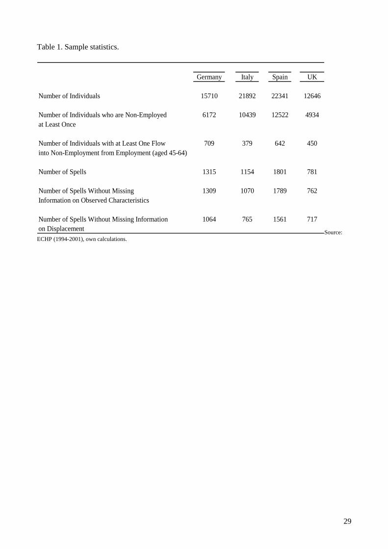
Table 1. Sample statistics.

Germany Italy Spain UK

Number of Individuals 15710 21892 22341 12646

Number of Individuals who are Non-Employed 6172 10439 12522 4934at Least Once

Number of Individuals with at Least One Flow 709 379 642 450into Non-Employment from Employment (aged 45-64)

Number of Spells 1315 1154 1801 781

Number of Spells Without Missing 1309 1070 1789 762Information on Observed Characteristics

Number of Spells Without Missing Information 1064 765 1561 717on Displacement Source:

ECHP (1994-2001), own calculations.

29

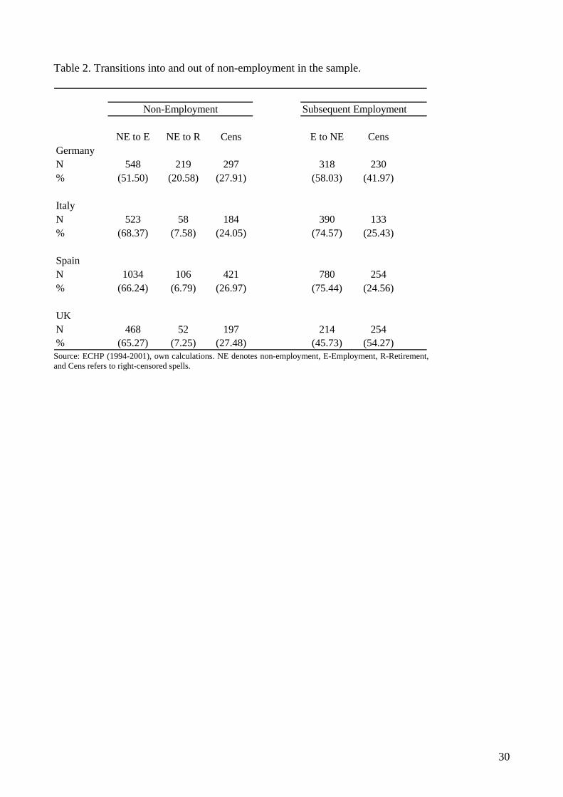
Table 2. Transitions into and out of non-employment in the sample.

NE to E NE to R Cens E to NE CensGermanyN 548 219 297 318 230% (51.50) (20.58) (27.91) (58.03) (41.97)

ItalyN 523 58 184 390 133% (68.37) (7.58) (24.05) (74.57) (25.43)

SpainN 1034 106 421 780 254% (66.24) (6.79) (26.97) (75.44) (24.56)

UKN 468 52 197 214 254% (65.27) (7.25) (27.48) (45.73) (54.27)

Non-Employment Subsequent Employment

Source: ECHP (1994-2001), own calculations. NE denotes non-employment, E-Employment, R-Retirement, and Cens refers to right-censored spells.

30

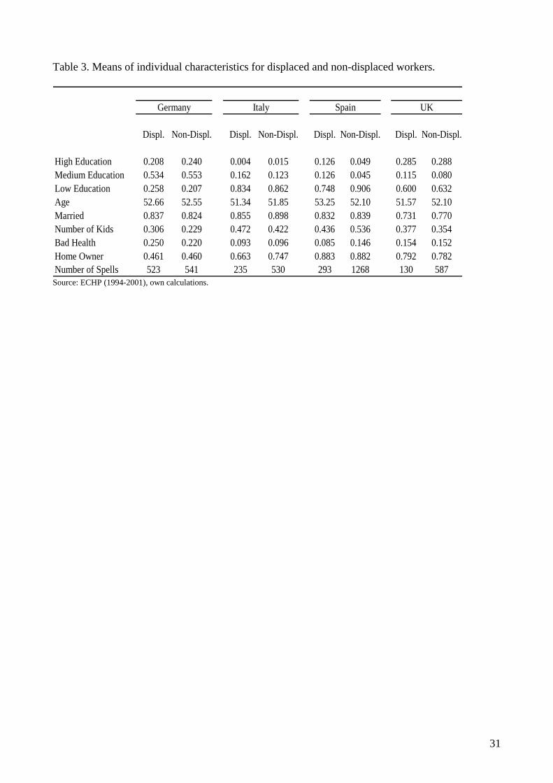
Table 3. Means of individual characteristics for displaced and non-displaced workers.

Displ. Non-Displ. Displ. Non-Displ. Displ. Non-Displ. Displ. Non-Displ.

High Education 0.208 0.240 0.004 0.015 0.126 0.049 0.285 0.288Medium Education 0.534 0.553 0.162 0.123 0.126 0.045 0.115 0.080Low Education 0.258 0.207 0.834 0.862 0.748 0.906 0.600 0.632Age 52.66 52.55 51.34 51.85 53.25 52.10 51.57 52.10Married 0.837 0.824 0.855 0.898 0.832 0.839 0.731 0.770Number of Kids 0.306 0.229 0.472 0.422 0.436 0.536 0.377 0.354Bad Health 0.250 0.220 0.093 0.096 0.085 0.146 0.154 0.152Home Owner 0.461 0.460 0.663 0.747 0.883 0.882 0.792 0.782Number of Spells 523 541 235 530 293 1268 130 587


Source: ECHP (1994-2001), own calculations.

31

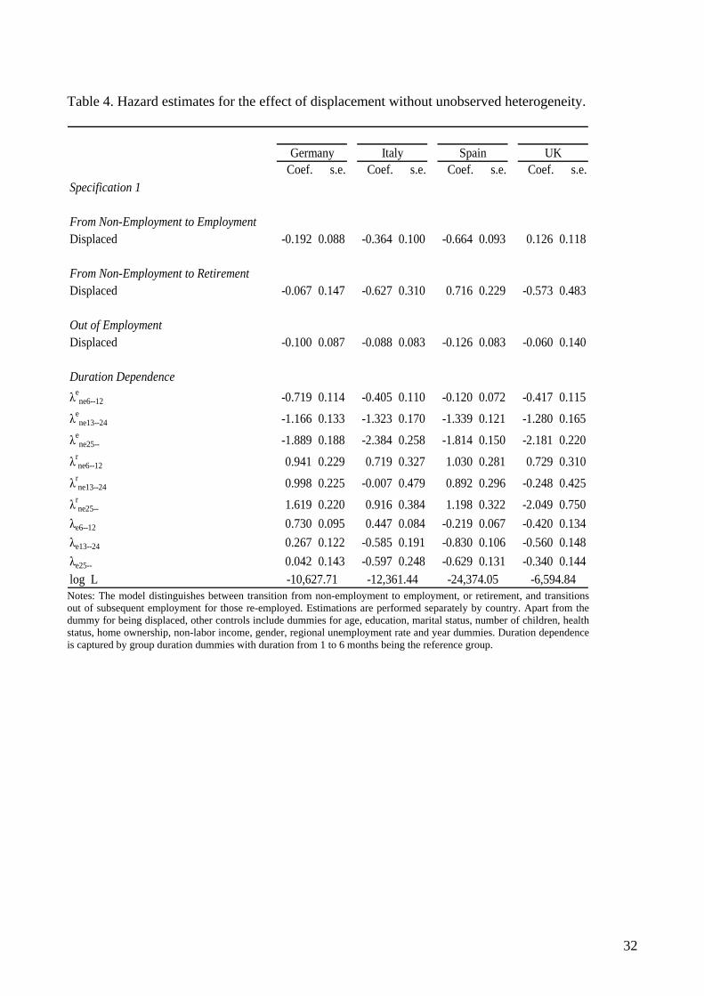
Table 4. Hazard estimates for the effect of displacement without unobserved heterogeneity.

Coef. s.e. Coef. s.e. Coef. s.e. Coef. s.e.Specification 1

Displaced -0.192 0.088 -0.364 0.100 -0.664 0.093 0.126 0.118

Displaced -0.067 0.147 -0.627 0.310 0.716 0.229 -0.573 0.483

Out of EmploymentDisplaced -0.100 0.087 -0.088 0.083 -0.126 0.083 -0.060 0.140

Duration Dependenceλe

ne6--12 -0.719 0.114 -0.405 0.110 -0.120 0.072 -0.417 0.115λe

ne13--24 -1.166 0.133 -1.323 0.170 -1.339 0.121 -1.280 0.165

λene25-- -1.889 0.188 -2.384 0.258 -1.814 0.150 -2.181 0.220

λrne6--12 0.941 0.229 0.719 0.327 1.030 0.281 0.729 0.310

λrne13--24 0.998 0.225 -0.007 0.479 0.892 0.296 -0.248 0.425

λrne25-- 1.619 0.220 0.916 0.384 1.198 0.322 -2.049 0.750

λe6--12 0.730 0.095 0.447 0.084 -0.219 0.067 -0.420 0.134λe13--24 0.267 0.122 -0.585 0.191 -0.830 0.106 -0.560 0.148λe25-- 0.042 0.143 -0.597 0.248 -0.629 0.131 -0.340 0.144log L


-24,374.05 -6,594.84

From Non-Employment to Retirement

From Non-Employment to Employment

-10,627.71 -12,361.44 Notes: The model distinguishes between transition from non-employment to employment, or retirement, and transitions out of subsequent employment for those re-employed. Estimations are performed separately by country. Apart from the dummy for being displaced, other controls include dummies for age, education, marital status, number of children, health status, home ownership, non-labor income, gender, regional unemployment rate and year dummies. Duration dependence is captured by group duration dummies with duration from 1 to 6 months being the reference group.

32

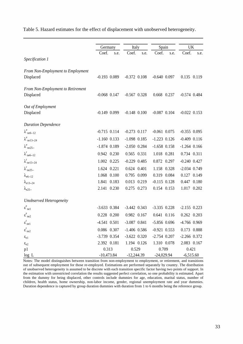
Table 5. Hazard estimates for the effect of displacement with unobserved heterogeneity.

Coef. s.e. Coef. s.e. Coef. s.e. Coef. s.e.Specification 1

Displaced -0.193 0.089 -0.372 0.108 -0.640 0.097 0.135 0.119

Displaced -0.068 0.147 -0.567 0.328 0.668 0.237 -0.574 0.484

Out of EmploymentDisplaced -0.149 0.099 -0.148 0.100 -0.087 0.104 -0.022 0.153


ne6--12 -0.715 0.114 -0.273 0.117 -0.061 0.075 -0.355 0.095

λene13--24 -1.160 0.133 -1.098 0.185 -1.223 0.126 -0.409 0.116

λene25-- -1.874 0.189 -2.050 0.284 -1.658 0.158 -1.264 0.166

λrne6--12 0.942 0.230 0.565 0.331 1.018 0.281 0.734 0.311

λrne13--24 1.002 0.225 -0.229 0.485 0.872 0.297 -0.240 0.427

λrne25-- 1.624 0.221 0.624 0.401 1.158 0.328 -2.034 0.749

λe6--12 1.068 0.100 0.795 0.099 0.319 0.084 0.127 0.149λe13--24 1.841 0.183 0.013 0.219 -0.115 0.128 0.447 0.180λe25-- 2.141 0.230 0.275 0.273 0.154 0.153 1.017 0.202

Unobserved Heterogeneityεe

ne1 -3.633 0.384 -3.442 0.343 -3.335 0.228 -2.155 0.223εe

ne2 0.228 0.200 0.982 0.167 0.641 0.116 0.262 0.203

εrne1 -4.541 0.501 -3.087 0.841 -5.856 0.696 -4.766 0.969

εrne2 0.086 0.307 -1.406 0.586 -0.921 0.553 0.173 0.888

εe1 -3.739 0.354 -3.622 0.320 -2.754 0.207 -2.266 0.372εe2 2.392 0.181 1.194 0.126 1.310 0.078 2.083 0.167p1log L -10,473.84 -12,244.39 -24,029.94 -6,515.60

0.709 0.421




0.313 0.529

Notes: The model distinguishes between transition from non-employment to employment, or retirement, and transitions out of subsequent employment for those re-employed. Estimations are performed separately by country. The distribution of unobserved heterogeneity is assumed to be discrete with each transition specific factor having two points of support. In the estimation with unrestricted correlation the results suggested perfect correlation, so one probability is estimated. Apart from the dummy for being displaced, other controls include dummies for age, education, marital status, number of children, health status, home ownership, non-labor income, gender, regional unemployment rate and year dummies. Duration dependence is captured by group duration dummies with duration from 1 to 6 months being the reference group.

33

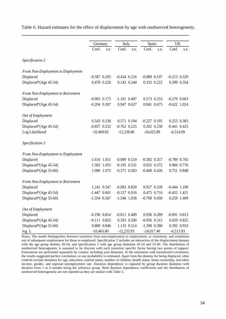
Table 6. Hazard estimates for the effect of displacement by age with unobserved heterogeneity.

Coef. s.e. Coef. s.e. Coef. s.e. Coef. s.e.

Specification 2

Displaced -0.587 0.205 -0.434 0.216 -0.889 0.197 -0.215 0.329Displaced*(Age 45-54) 0.478 0.226 0.142 0.244 0.333 0.222 0.399 0.354

Displaced -0.005 0.175 -1.161 0.497 0.573 0.253 -0.270 0.663Displaced*(Age 45-54) -0.204 0.307 0.947 0.637 0.841 0.675 -0.622 1.024

Out of EmploymentDisplaced 0.543 0.236 0.571 0.194 -0.227 0.195 0.253 0.383Displaced*(Age 45-54) -0.857 0.252 -0.762 0.225 0.202 0.230 -0.441 0.425Log Likelihood

Specification 3

Displaced -1.610 1.051 -0.089 0.519 -0.582 0.357 -0.789 0.765Displaced*(Age 45-54) 1.502 1.055 -0.195 0.531 0.025 0.372 0.984 0.776Displaced*(Age 55-60) 1.086 1.072 -0.571 0.563 -0.408 0.426 0.751 0.848

Displaced 1.241 0.547 -0.083 0.820 0.927 0.339 -0.444 1.190Displaced*(Age 45-54) -1.447 0.601 -0.127 0.916 0.475 0.716 -0.455 1.421Displaced*(Age 55-60) -1.354 0.567 -1.546 1.036 -0.708 0.450 0.259 1.409

Out of EmploymentDisplaced -0.196 0.814 -0.811 0.489 0.936 0.289 -0.091 0.813Displaced*(Age 45-54) -0.111 0.825 0.593 0.500 -0.956 0.315 0.029 0.825Displaced*(Age 55-60) 0.808 0.846 1.133 0.514 -1.398 0.380 0.392 0.933log L



-10,469.82 -12,238.80

-10,463.80 -12,233.93 -24,017.40 -6,513.93

-24,025.89 -6,514.09




Notes: The model distinguishes between transition from non-employment to employment, or retirement, and transitions out of subsequent employment for those re-employed. Specification 2 includes an interaction of the displacement dummy with the age group dummy 45-54, and specification 3 with age group dummies 45-54 and 55-60. The distribution of unobserved heterogeneity is assumed to be discrete with each transition specific factor having two points of support. Estimations are performed separately by country including year dummies. In the estimation with unrestricted correlation, the results suggested perfect correlation, so one probability is estimated. Apart from the dummy for being displaced, other controls include dummies for age, education, marital status, number of children, health status, home ownership, non-labor income, gender, and regional unemployment rate. Duration dependence is captured by group duration dummies with duration from 1 to 6 months being the reference group. Both duration dependence coefficients and the distribution of unobserved heterogeneity are not reported as they are similar with Table 5.

34

Table 7. Hazard estimates for the effect of displacement with unobserved heterogeneity controlling for the endogeneity of displacement.


Specification 1Displaced -0.175 0.105 0.180 0.156 -0.365 0.107 0.124 0.118

Specification 2Displaced -0.584 0.213 0.012 0.246 -0.619 0.200 -0.208 0.331Displaced*(Age 45-54) 0.489 0.225 0.209 0.235 0.332 0.219 0.403 0.356

Specification 3Displaced -1.610 1.052 0.686 0.545 -0.292 0.359 -0.769 0.762Displaced*(Age 45-54) 1.516 1.055 -0.338 0.545 0.002 0.369 0.968 0.774Displaced*(Age 55-60) 1.090 1.072 -0.653 0.577 -0.451 0.422 0.728 0.845

Specification 1Displaced -0.105 0.180 -0.578 0.532 0.340 0.259 -0.576 0.484

Specification 2Displaced -0.041 0.201 -1.190 0.621 0.210 0.272 -0.264 0.664Displaced*(Age 45-54) -0.198 0.306 1.018 0.616 0.951 0.675 -0.636 1.024

Specification 3Displaced 1.209 0.553 -0.335 0.824 0.572 0.359 -0.417 1.184Displaced*(Age 45-54) -1.446 0.601 0.012 0.880 0.598 0.716 -0.473 1.418Displaced*(Age 55-60) -1.359 0.567 -1.521 1.014 -0.647 0.448 0.200 1.402

Out of EmploymentSpecification 1Displaced -0.707 0.126 0.356 0.100 0.381 0.098 -0.159 0.164

Specification 2Displaced -0.366 0.294 0.555 0.207 0.281 0.172 0.205 0.398Displaced*(Age 45-54) -0.391 0.309 -0.347 0.196 0.140 0.197 -0.265 0.433

Specification 3Displaced -0.722 0.823 0.034 0.424 0.427 0.162 -0.144 0.815Displaced*(Age 45-54) -0.039 0.822 0.223 0.424 0.462 0.161 0.289 0.826Displaced*(Age 55-60) 0.401 0.856 0.681 0.450 -0.203 0.135 0.444 0.932




Notes: See notes in Table 6. The model is extended by estimating the probability to be displaced. The unobserved factor is allowed to be correlated with the transition equations.

35

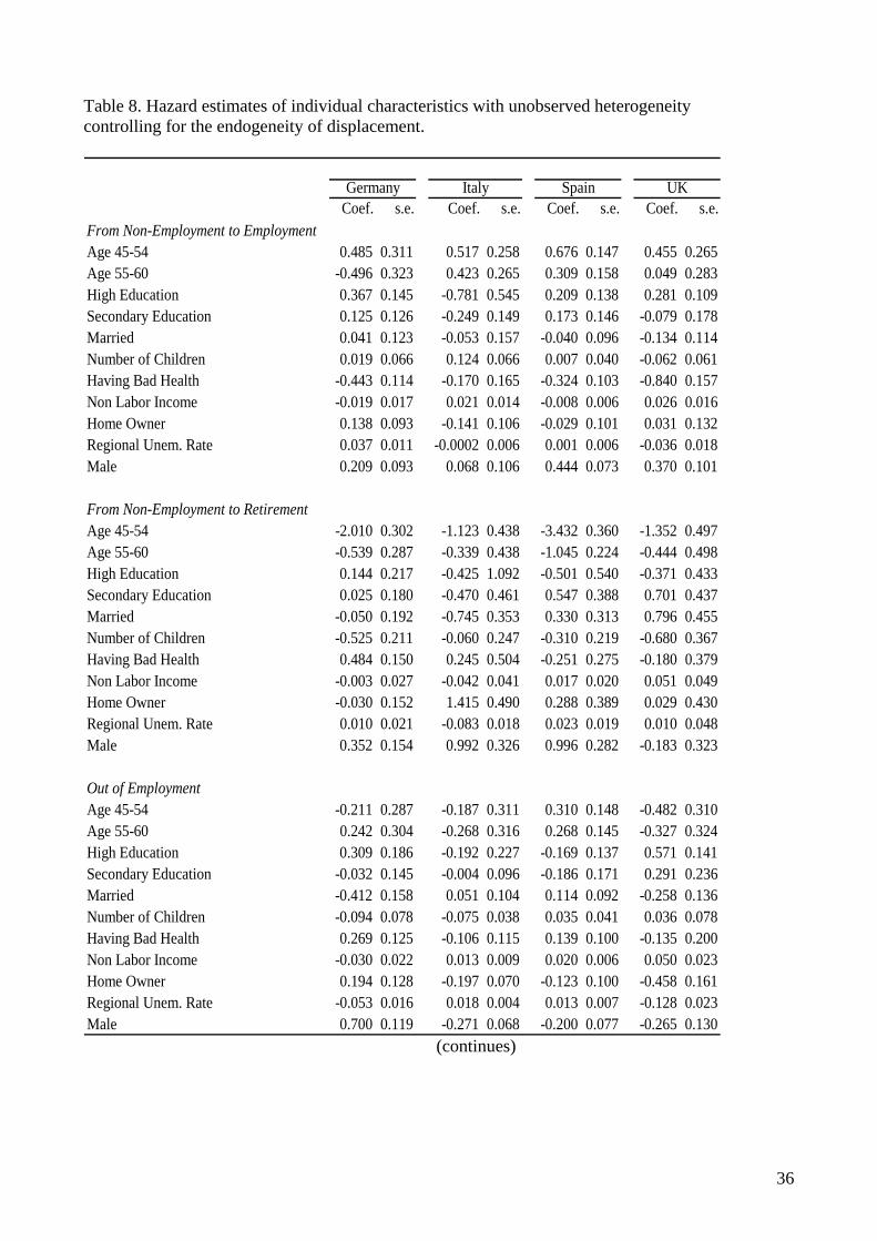
Table 8. Hazard estimates of individual characteristics with unobserved heterogeneity controlling for the endogeneity of displacement.


Age 45-54 0.485 0.311 0.517 0.258 0.676 0.147 0.455 0.265Age 55-60 -0.496 0.323 0.423 0.265 0.309 0.158 0.049 0.283High Education 0.367 0.145 -0.781 0.545 0.209 0.138 0.281 0.109Secondary Education 0.125 0.126 -0.249 0.149 0.173 0.146 -0.079 0.178Married 0.041 0.123 -0.053 0.157 -0.040 0.096 -0.134 0.114Number of Children 0.019 0.066 0.124 0.066 0.007 0.040 -0.062 0.061Having Bad Health -0.443 0.114 -0.170 0.165 -0.324 0.103 -0.840 0.157Non Labor Income -0.019 0.017 0.021 0.014 -0.008 0.006 0.026 0.016Home Owner 0.138 0.093 -0.141 0.106 -0.029 0.101 0.031 0.132Regional Unem. Rate 0.037 0.011 -0.0002 0.006 0.001 0.006 -0.036 0.018Male 0.209 0.093 0.068 0.106 0.444 0.073 0.370 0.101

Age 45-54 -2.010 0.302 -1.123 0.438 -3.432 0.360 -1.352 0.497Age 55-60 -0.539 0.287 -0.339 0.438 -1.045 0.224 -0.444 0.498High Education 0.144 0.217 -0.425 1.092 -0.501 0.540 -0.371 0.433Secondary Education 0.025 0.180 -0.470 0.461 0.547 0.388 0.701 0.437Married -0.050 0.192 -0.745 0.353 0.330 0.313 0.796 0.455Number of Children -0.525 0.211 -0.060 0.247 -0.310 0.219 -0.680 0.367Having Bad Health 0.484 0.150 0.245 0.504 -0.251 0.275 -0.180 0.379Non Labor Income -0.003 0.027 -0.042 0.041 0.017 0.020 0.051 0.049Home Owner -0.030 0.152 1.415 0.490 0.288 0.389 0.029 0.430Regional Unem. Rate 0.010 0.021 -0.083 0.018 0.023 0.019 0.010 0.048Male 0.352 0.154 0.992 0.326 0.996 0.282 -0.183 0.323

Out of EmploymentAge 45-54 -0.211 0.287 -0.187 0.311 0.310 0.148 -0.482 0.310Age 55-60 0.242 0.304 -0.268 0.316 0.268 0.145 -0.327 0.324High Education 0.309 0.186 -0.192 0.227 -0.169 0.137 0.571 0.141Secondary Education -0.032 0.145 -0.004 0.096 -0.186 0.171 0.291 0.236Married -0.412 0.158 0.051 0.104 0.114 0.092 -0.258 0.136Number of Children -0.094 0.078 -0.075 0.038 0.035 0.041 0.036 0.078Having Bad Health 0.269 0.125 -0.106 0.115 0.139 0.100 -0.135 0.200Non Labor Income -0.030 0.022 0.013 0.009 0.020 0.006 0.050 0.023Home Owner 0.194 0.128 -0.197 0.070 -0.123 0.100 -0.458 0.161Regional Unem. Rate -0.053 0.016 0.018 0.004 0.013 0.007 -0.128 0.023Male 0.700 0.119 -0.271 0.068 -0.200 0.077 -0.265 0.130




(continues)

36

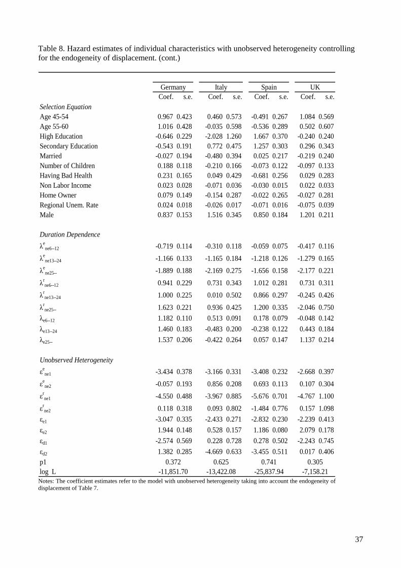
Table 8. Hazard estimates of individual characteristics with unobserved heterogeneity controlling for the endogeneity of displacement. (cont.)

Coef. s.e. Coef. s.e. Coef. s.e. Coef. s.e.Selection EquationAge 45-54 0.967 0.423 0.460 0.573 -0.491 0.267 1.084 0.569Age 55-60 1.016 0.428 -0.035 0.598 -0.536 0.289 0.502 0.607High Education -0.646 0.229 -2.028 1.260 1.667 0.370 -0.240 0.240Secondary Education -0.543 0.191 0.772 0.475 1.257 0.303 0.296 0.343Married -0.027 0.194 -0.480 0.394 0.025 0.217 -0.219 0.240Number of Children 0.188 0.118 -0.210 0.166 -0.073 0.122 -0.097 0.133Having Bad Health 0.231 0.165 0.049 0.429 -0.681 0.256 0.029 0.283Non Labor Income 0.023 0.028 -0.071 0.036 -0.030 0.015 0.022 0.033Home Owner 0.079 0.149 -0.154 0.287 -0.022 0.265 -0.027 0.281Regional Unem. Rate 0.024 0.018 -0.026 0.017 -0.071 0.016 -0.075 0.039Male 0.837 0.153 1.516 0.345 0.850 0.184 1.201 0.211


ne6--12 -0.719 0.114 -0.310 0.118 -0.059 0.075 -0.417 0.116

λene13--24 -1.166 0.133 -1.165 0.184 -1.218 0.126 -1.279 0.165

λene25-- -1.889 0.188 -2.169 0.275 -1.656 0.158 -2.177 0.221

λrne6--12 0.941 0.229 0.731 0.343 1.012 0.281 0.731 0.311

λrne13--24 1.000 0.225 0.010 0.502 0.866 0.297 -0.245 0.426

λrne25-- 1.623 0.221 0.936 0.425 1.200 0.335 -2.046 0.750

λe6--12 1.182 0.110 0.513 0.091 0.178 0.079 -0.048 0.142λe13--24 1.460 0.183 -0.483 0.200 -0.238 0.122 0.443 0.184λe25-- 1.537 0.206 -0.422 0.264 0.057 0.147 1.137 0.214

Unobserved Heterogeneityεe

ne1 -3.434 0.378 -3.166 0.331 -3.408 0.232 -2.668 0.397

εene2 -0.057 0.193 0.856 0.208 0.693 0.113 0.107 0.304

εrne1 -4.550 0.488 -3.967 0.885 -5.676 0.701 -4.767 1.100

εrne2 0.118 0.318 0.093 0.802 -1.484 0.776 0.157 1.098

εe1 -3.047 0.335 -2.433 0.271 -2.832 0.230 -2.239 0.413εe2 1.944 0.148 0.528 0.157 1.186 0.080 2.079 0.178εd1 -2.574 0.569 0.228 0.728 0.278 0.502 -2.243 0.745εd2 1.382 0.285 -4.669 0.633 -3.455 0.511 0.017 0.406p1log L

Spain UKGermany Italy

0.741 0.305-11,851.70 -13,422.08 -25,837.94 -7,158.21

0.372 0.625

Notes: The coefficient estimates refer to the model with unobserved heterogeneity taking into account the endogeneity of displacement of Table 7.

37

the effect of job displacement on the transitions to ...ftp.iza.org/dp3069.pdfthe effect of job...

Documents