The Effect of Mexico’s Conditional Cash Transfer Program on

Migration Decisions

Aki Ishikawa1

Professor Charles Becker, Faculty Advisor

Duke University

Durham, North Carolina

2014

                                                                                                               1 Aki Ishikawa graduated in May 2014 with Distinction in Economics and a minor in Spanish. Following graduation, Aki will be working at Deloitte Tax LLP as a Consultant for the Transfer Pricing Group in the Chicago office. Aki can be reached at Aki.Ishikawa105@gmail.com.

Ishikawa 2  

Acknowledgements I would like to thank my advisor, Professor Charles Becker, for his patience, guidance,

optimism, and support throughout this challenging process. I would also like to thank Professor

Kent Kimbrough and Professor Michelle Connolly for their constructive feedback and comments

on my presentations and numerous drafts. Last but not least, I am very thankful for my peers in

the Honors Thesis Seminars for their input and advice.

Ishikawa 3  

Abstract The Mexican conditional cash transfer program, Oportunidades, is commonly overlooked

for long-term evaluations. One understudied effect of this poverty-reduction program is the

change in migration behavior caused by the cash transfers. Using data from the Mexican Family

Life Survey, this study outlines the effects of the social net program on international migration of

low-income households in Mexico. The results suggest that the program causes a positive

increase in likelihood for international migration for program participants. Within participating

households, individuals who are responsible for grant income tend to migrate less compared to

the other members of the households. This research provides valuable insight into existing

literature on migration of low-income households in relation to the availability of the conditional

cash transfer program.

Ishikawa 4  

Introduction

Many developing countries often times suffer a troubling issue known as the

intergenerational poverty trap. A poverty trap is a self-enforcing cycle and occurs when

households in poverty continue to remain poor due to the lack of resources or opportunities that

enable its citizens to escape. Recently, some developing countries implemented conditional cash

transfer programs as possible solutions to eliminate the poverty trap for low-income households.

A conditional cash transfer program is very simple in structure: eligible households receive a

cash reward contingent on the households sending their children to school and attending health

clinic sessions. By providing monetary incentives, this social net program motivates children to

gain resources to accumulate human capital through education and health interventions in hopes

that these children will be able to escape poverty. For example, in 2003, the Brazilian

government successfully initiated the Bolsa Familia conditional cash transfer program that

allowed program participants to receive a monthly stipend if families enrolled their children in

school and younger children received a set of vaccinations (Paes-Sousa, Santos, & Miazaki,

2011). The popularity of the conditional cash transfer program has grown, and similar programs

have sprouted across many developing Latin American countries including Chile, Colombia,

Honduras, and Guatemala.

The effects of the conditional cash transfer on participating households are multi-

dimensional and have been a field of interest for many economic research studies. Most studies

have evaluated the short-term effects of the program, such as educational attainment and health

outcomes of the children soon after the program’s implementation, but little literature evaluates

its long-term effects. One such understudied household characteristic is the program’s effects on

migration. The conditional cash transfer programs have the potential to target extensive

Ishikawa 5  

populations of poverty-stricken families who may already engage in migration. The interaction

between migration and this social net program is understudied. To explain, the cash transfers

alter the household budgets of low-income families: additional wealth may lower the cost of

migration and allow family members to migrate easier. On the other hand, participation may

discourage migration by incentivizing the family members to stay to meet the program’s

requirements. This study will add to the literature on migration studies by evaluating migration

of individuals who participate in the conditional cash transfer program using data from Mexico, a

country with both well-studied migration data and one of the oldest conditional cash transfer

programs, Oportunidades.

Oportunidades Background

Formerly known as Progresa, Oportunidades began in 1997, and is one of the most

important pilot conditional cash transfer programs (CCT) in the world. The program was first

offered to rural communities, and as the program became more widely accepted, the CCT

program gradually expanded to urban communities, increasing the number of program

beneficiaries. By 2007, the program reported that over five million families, or roughly 18% of

the country’s total population were benefiting from the cash transfer program (Fiszbein, Schady,

& Ferreira, 2009). The program has been noted to be very successful, improving conditions for

program beneficiaries. Previous research has shown that the program decreased child labor, and

increased enrollment in schools (Skoufias, Parker, Behrman, & Pessino, 2001). Studies also

have discovered that the CCT increased birth weight for infants, improving health outcomes

(Barber & Gertler, 2008) and decreasing infant mortality (Barham, 2011). The success of the

Mexican CCT program inspired other Latin American CCT’s to adopt its program design in

launching their respective programs.

Ishikawa 6  

The program is crafted to stimulate human capital accumulation through education and

improving health of children of participating households through requirements imposed on

children’s school attendance, family’s health clinic attendance, and nutrition session attendance

for mothers with young children. The program requires participation from all of the household

members. First, an eligible household must send all of its children to local schools in order to

meet the education attendance requirement. The World Bank reports that the benchmark

attendance rate for an individual child is roughly around 80% monthly and 93% annually for all

schools, and the education requirement applies until the children graduate from high school (The

World Bank Group)2. Also, the entire family must attend a required number of medical

checkups at the local clinic every year and if a household member is older than 15, that

household member must attend an additional health and nutritional lecture. Finally, for pregnant

mothers and young children between the ages of four months and four years, the program will

give out nutritional supplements and food grants.

Oportunidades Eligibility

The program selection was based on the set of criteria chosen to identify families with the

most severe poverty trap. First, the program isolated cities or towns by constructing a

marginality index to identify those with the highest poverty rates (Skoufias, Davis, & de la Vega,

2001). The marginality index was constructed through using data from the 1990 Mexican census

on population and housing (ENCASH) and 1995 population and housing count conducted by the

Mexican national statistics institute (INEGI). Cities or towns that met the target poverty rates

were included in the program based on size and availability of facilities and access to services.

                                                                                                               2 This information is as of 2007.

Ishikawa 7  

Next, each city or town identified poor households by comparing household income per capita

against an average household’s income.

In the initial analysis conducted in 1997, the program randomized 505 rural communities

with 24,077 households to test the program’s efficiency (Skoufias, Davis, & de la Vega, 2001).

In 1998, the program assigned 320 cities as treatment and 185 cities as control (Behrman &

Todd, 1999) . Each treatment group contacted all eligible, poor households and offered the

program while all control groups were left alone. By randomizing at the city level, the study

controlled for possible household spillover effects within the same city. After an extensive

evaluation of the program, the Mexican government expanded the CCT to cover more

households, including those in urban communities beginning in 2000.

If the family is determined to be eligible, the program notifies the family, and the family

registers all of its members to the program (Skoufias, Davis, & de la Vega, 2001). The program

is a community-wide effort in which local health clinics and schools are assigned to the family,

and local officials record the appropriate attendance measures for the household. The

information is verified bimonthly, and once the family meets the necessary requirements, an

appropriate grant is sent to a payment center. In order to access the grant money, mothers or

caretakers of the households are required to register with the payment center, and they are the

only ones who can access the money. Access is granted to women to encourage empowerment

of women in these households.

Ishikawa 8  

Oportunidades Grant Details

Table 1 above provides a brief summary of what each household is expected to receive

for the most recent year, 2013. If school attendance is met by all of the children and they

successfully graduate, the household is awarded a graduation grant for each child. The

compliance for the program is very high, and according to the World Bank Group, 98% of

beneficiary families receive benefits from the program ("Support to Oportunidades Project,"

2013).

                                                                                                               3 Source: Oportunidades.gob.mx. USD/MXN=12.96 as of July 1st, 2013.

Grade Monetary Benefits per child3

Primary $165 -330/ mo., $410/year for supplies

Secondary $485- 620/ mo., $415/year for supplies

Middle/Higher $810- 1055/mo., $415/year for supplies

Nutrition $115- 345/ household

Graduation $4,599- 5,956/ child (for all children)

Table 1: Cash Grant Summary for Oportunidades in 2013 Mexican Pesos

Ishikawa 9  

375

400

425

450

475

500

525

550

575

600

625

Am

ount

in

Peso

s

Year

Figure 2a: Trends in Secondary Education Cash Grants per child per month, in 2010 Mexican real pesos

First Year Men First Year WomenSecond Year Men Second Year WomenThird Year Men Third Year Females

-

100

200

300

400

500

600

700

800

900

1,000

1,100

1,200

1,300

20112010200920082007200620052004200320022001200019991998

Am

ount

in

Peso

s

Year

Figure 1: Summary of trends of different cash grants amounts per household per month, in 2010 Mexican real Pesos

Nutrition Grant Supplies Grant Max Education Grant per family

Ishikawa 10  

600

750

900

1,050

1,200

1,350

1,500

1,650

1,800

2012201120102009200820072006200520042003200220012000199919981997

Am

ount

in

Peso

s

Year

Figure 2b: Trends in Higher Education Cash Grants per child per month, in 2010 Mexican real pesos

First Year Men First Year WomenSecond Year Men Second Year WomenThird Year Men Third Year Women

The above three figures represent the general trends seen in the cash grants per household

per month from the program. The data source is from oportunidades.gob.mx, the official

government reporting of the CCT. The cash grants received from a child in primary school is not

pictured above. Figure 1 illustrates the division of the monthly disbursement amount in Mexican

pesos for an eligible household in the program. The nutrition support grant is for pregnant and

young children who meet the eligibility for the households. The supplies grant shown in Figure

1 is a cash grant for school supplies given out annually to a child studying in secondary and

higher education schools. The maximum education grant is the maximum amount that the

family with a child studying in either primary or secondary school can receive in a month.

Looking at the figure, the education grant is the largest source of grant income.

Ishikawa 11  

Figures 2a and 2b further decompose the possible education grant for each eligible child

sorted by year of study, school, and gender. Across both secondary and higher education levels,

female students always receive more than compared to their respective male counterparts. This

differential in disbursements represents the program’s intention to reward families who educate

girls, who are usually under-represented in the schooling system. The value of the grant

increases as the level of schooling increases as well. The possible higher education grants that a

child can receive seem to have decreased over the years while secondary education grants seem

stable. This difference in this trend has not been noted in any of the program’s analyses.

Given the program’s grant composition, the grant income may differ depending on the

characteristics of the children and other household members. The range of the monetary value of

the cash grants vary, and can have different proportions compared to the household income. This

study will hypothesize that this impact on the household’s monthly budget is substantial enough

to change household behavior and would like to incorporate the grant income into the analyses.

Migration Theories and Literature Review

The characteristics of the Oportunidades program and migration theories can be

combined to infer the migration behaviors of household members who are program recipients.

Very few studies have evaluated the program recipients’ migration patterns, but there exist many

theories and research that have studied low-income households, similar to the program’s

recipients. It is important to understand the underlying motivation for migration of low-income

households to infer on how the program may alter the existing motivators for such individuals.

This following section briefly summarizes migration findings for households that closely

resemble what the Oportunidades targets.

Ishikawa 12  

The literature and theories behind migration decisions can be broadly divided into the

neoclassical theory, new economics of labor migration theory, and social network theory

(Lindstrom & Lauster, 2001). To begin, neoclassical scholars believe that the household and

individual migration decisions occur based on the incentive to maximize individual or household

utilities. Among the neoclassical migration theories, Harris and Todaro’s migration theory states

that an individual’s migration decision is influenced by the wage differential represented in rural

or urban districts or between two different locations (Harris & Todaro, 1970). If a labor

opportunity in another region outside of the individual’s current position is more attractive, and

if the gains from migration outweigh the costs incurred, the individual is more likely to migrate.

Similarly, Sajaastad’s model for costs and returns on human migration articulates that an

individual migrates if returns from the new work opportunity are significantly greater than the

costs incurred due to relocation, then the individual is more likely to migrate (Sjaastad, 1962).

More recently, however, Stiglitz has updated this approach adding that the difference in wage

between rural and urban labor is explained by the premium on labor skills and turnover in the

urban sector (Stiglitz, 1974). His theory suggests that the unemployment rate and urban wage

rate are endogenous, and competitive firms are incentivized to pay premiums to attract labor,

attributing to the wage differential. This implies that this perceived wage differential is not the

only driving determinant of migration.

Next, new economics of labor migration theory shows a different perspective. In this

theory, an individual’s migration is heavily influenced by the household’s utility optimization. In

this approach, the migrant moves to work in order to send a part of the earnings in remittances

back to the rest of the household (Stark & Lucas, 1988). Stark’s migration model applies

primarily to agricultural households with less access to credit. Such household can alleviate the

Ishikawa 13  

credit constraint through sending one of its members to earn money. These earnings are used to

help the household meet current consumption needs that include food, basic health services,

consumer goods, and housing needs (Conway & Cohen, 1998). The additional income can act as

insurance and allow the household to make additional investments elsewhere such as that in

agricultural production.

Another migration theory that has gained momentum is social network theory. The social

network theory outlines the idea that people are more likely to migrate if they have a working

kinship network at the intended location of migration (Taylor, 1986). For risk-averse households,

sending a household member to migrate is a very risky decision. If the household knows

someone such as a relative at the intended location of migration, the theory suggests that the

household member will be more likely to migrate. By having a connection, the household can

gain valuable information that may decrease risk and uncertainty. The theory also indicates that

the role of networks is especially strong for international migration for households in developing

countries.

The overall migration literature is extensive. Aside from the theories noted earlier, crime

and violence may be strong indicators for predicting migration of individuals in Mexico. An

increase in migration was seen with higher reported violent incidences of homicide and guerilla

attacks (Grun, 2009). Migration and labor market participation is closely linked and high levels

of violence can decrease participation in the labor market for self-employed men and single

women (Velásquez, 2014). Velásquez’s research shows that high rates of homicide increase the

possibility of victimization through extortion and theft added to the cost of participating in the

labor market, motivating these individuals to migrate.

Ishikawa 14  

Numerous studies have explored the application of these migration theories to households

in developing countries. Many literature sources suggest that low-income households decide to

migrate for better wages or work opportunities or location specific characteristics (Dostie &

Léger, 2009). These migrant workers are commonly influenced by work opportunities that may

allow them to sustain their families’ current consumptions (Conway & Cohen, 1998). An

individual migrates not only to improve the absolute household income but also the relative

standing of the household’s income compared to other similar households in the same

community (Stark & Taylor, 1991). Low-income households are more likely to engage in

international migration than compared to high-income households in the same community.

Related, less educated individuals migrate internationally to the US while more educated

individuals tend to stay within Mexico. Stark and Taylor conducted this study prior to the

induction of the Oportunidades program, but can provide information that may be useful in

analyzing participating households. Another study by Lindstrom and Lauster evaluates the

application of all of the migration theories to a Mexican community and determines the

likelihoods of internal migration and US migration (Lindstrom & Lauster, 2001). The model’s

outcomes follow that of predicted values and directions stated in the neoclassical, new

economics, and social network theory of migration. This study would like to evaluate the

validity of these migration theories with the effects due to Oportunidades.

One study has specifically looked into migration of Oportunidades grant recipients in the

program’s early years. Stecklov et al.’s study evaluates migration between program participants

and non-program participants of similar background (Stecklov, Winters, Stampini, & Davis,

2005). Families perceived the cash grant to be an additional opportunity cost that the family

would need to give up for migration. On the other hand, the grant income may decrease the

Ishikawa 15  

actual cost to migrate. The study uses a difference-in-difference approach to measure the net

effect of the treatment on two types of migration: domestic migration and international migration

to the US. Stecklov et al’s study concludes that the grant increased international migration for

middle-aged women and increased domestic migration for people from large families. The

evaluation was conducted soon after the introduction of the program, and the possible long-term

participation may not be accounted for. This study would like to articulate and identify certain

members of the household and their different migration under the CCT program.

Comparing the existing literature on migration theories and the characteristics of the

conditional cash transfer program, the theoretical effects from the Oportunidades program can be

inferred. I would like to test two hypotheses about the grant’s impact on migration. First, I

would like to determine the net effect of program participation on migration compared to

households without the grant. Second, within participating households, I would like to evaluate

the likelihood of migration amongst different types of members.

The direct grant receivers are children, mothers, or primary care givers who need to be

present to participate in the program. From a cost-benefit approach, if the direct grant recipients

were to migrate, the household faces a risk of losing the grant income, adding to the cost of

migration for these members. This will also make it less likely for these individuals to migrate.

On the other hand, the grant income from Oportunidades may help household members who are

not direct grant receivers thinking of migrating to alleviate the costs associated with migration.

Specifically, household members such as older graduated children or other adults may move out

to work in order to send remittances for credit-constrained households, as explained in the new

economics of migration theories. The grant income may incentivize such individuals to migrate.

The program also mandates that all household adults need to attend a yearly health clinic

Ishikawa 16  

appointment in order to meet the attendance requirement for the grant. This requirement may

dissuade household members from moving far; thus, may be dissuaded to migrate far in risk of

losing the grant. Overall, the theoretical predictions indicate that the grant may facilitate or deter

migration in participating households depending on the type of individual.

Data

This research will use the dataset from the Mexican Family Life Survey (MxFLS)

conducted by the Institute of Geography Statistics and Information (INEGI). The survey is a

nationally representative, longitudinal database with approximately 8,440 households and 35,000

individuals. The MxFLS conducted the first wave in 2002 and resurveyed the same sample for

the second wave in 2005. The households sampled in the survey were randomized and based on

pre-selected demographic variables to create a nationally representative sample. According to

the survey codebook, the sampling framework for the survey subjects follow that of the 2002

Mexican National Employment Survey (Rubalcava & Teruel, 2006).

The MxFLS dataset was chosen because the surveys were originally aimed to track

households and individuals through a 10-year span through collecting data from three different

levels: community or region, household, and individual. The topics covered are very broad and

include socioeconomic indicators, income levels, education, migration, household assets and

much more. International migration incidences from Mexico and US are reported for individuals

who were present in the study at 2002 but had migrated when resurveyed in 2005. The study

will use the 2002 wave of this household survey to draw information about the international

migrants before their migration.

Most importantly, the dataset identifies households and individuals who are recipients of

the grant from the Oportunidades program, and reports the average annual income received from

Ishikawa 17  

the program. The data were collected four to five years after the start of the program, and can

represent the long-term exposure to the program. In the 2002 wave, a total of 1,117 households

stated they receive the grant from the program with a total of 6,235 individuals belonging to

these households.

The following figure represents the geographical distribution of the grant-receiving

households by states compared to the 2001 national grant disbursements released by the

Oportunidades program. At glance, the MxFLS survey seems to contain program participants at

a similar pattern of distribution as represented in the nationwide distribution. The MxFLS

survey also does not collect data from every state in Mexico: the data only include information

from 16 out of the 32 states in Mexico. Both the nationwide program participants’ distribution

and surveyed program participants’ distribution show a high density of grant-receiving

households in the southern states4. This distribution is similar to that of the national distribution

of households in poverty, which suggests that the survey does reflect the trends in the program.

The models will try to control for differences in regional distribution by adding state dummies

and cluster the standard errors by municipality.

                                                                                                               4 National disbursement data taken from oportunidades..gob.mx for September to October 2001

Ishikawa 18  

Next, the characteristics of the individual grant-receivers were analyzed to check if the

program design is effective in achieving its stated goals. The dataset contains two different types

of responses on grant participation and income: the household head’s responses on behalf of the

household and responses from individual family members’ responses. The data contained

discrepancies across household-level and individual-level responses for each household. In some

occasions, individuals in a household would report participation in Oportunidades but the

household-level data denied participation. This could suggest that the responders for the

household level data are not always aware of all of the household’s income sources or

individuals who responded as program participants could hide that information from the

household head. For these reasons, this study will label households as participants if the

household head replied indicated participation, and if household head replied no participation but

an individual of that household had indicated participation. Of the 946 individuals who are

Figure 3: Comparison of Nationwide and Surveyed Program Participants Distributions

Ishikawa 19  

program participants, 119 individuals belong to households who on the household level data

indicated were not program participants.

To properly find annual grant income per household, the responses of the family

members were analyzed to verify whether the reported grant income was aligned with the

program’s intentions. Only adults over the age of 15 were allowed to report participation and

grant income from the program. This group included 778 women and 168 men who reported

that they earned the grant income. Men reporting the income is puzzling, since the program gave

women access to program funding. The men were further evaluated, and 114 indicated that they

were sons in the family, whereas among women, 175 indicated that they were daughters in the

household. The program only allows mothers of households to access to money; however, the

survey shows other members reporting income, suggesting that the sons and daughters are aware

of the grant income total, but does not imply they have access to the money. Since all individuals

over the age of 15 reported in this survey, students who had attended school at the time of the

survey and had participated in the program are indicating that they had earned the grant income.

To eliminate confusion, the household head’s response on grant income will be used as the total

annual income the household received from Oportunidades.5

As for the dataset on migration, the MxFLS survey contains a separate set of responses

for individuals who have migrated to the US between the 2002 wave and 2005 wave. These

individuals were surveyed in 2002 but during the survey in 2005, had migrated to the US.

Between 2002 and 2005, 854 people out of the roughly 35,000 individuals migrated

internationally, roughly 2.4% of the sample (Appendix A).

                                                                                                               5 For models using grant income, the sample of individuals participating in the program whose household heads did not respond with an annual grant income or were unaware of program participation will be recorded as receiving no income from the program.

Ishikawa 20  

Empirical Specification

This study’s main interest is to evaluate the possible effects that the Oportunidades

program may have on the migration decisions of household participants. In the migration

literature, the model that most adequately captures this outcome is the logit model. The decision

on whether or not to migrate is binary, and this model captures the effect of certain

characteristics on the migration likelihood for the individual. This study will adopt a similar

model approach in order to measure the program’s effect on an individual’s migration.

This model’s outcome will be whether or not the individual migrated to the US sometime

between 2002 and 2005, given the characteristics reported about the individual in 2002. The

independent variables are from 2002 to avoid possible reverse causality. The following model

represents the migration outcome against the characteristics:

  1        !"#$% !!" =  ! + !!"#!!"#

!

!!!

+ !!"

!

!!!

!!" + ℎℎ!"#$%! + !!

!"

!!!

!!   +  !!"

The outcome of this model is binary indicator with value of 1 for migration to the US for

individual i from household j. Individual-level characteristics (X) are include age, age-squared,

gender and last completed education level. The dataset does not report the number of years in

school and will instead use education levels, sorted into three binary variables of the following

categories: no education, secondary and high school completion. Primary schooling is omitted to

prevent multicollinearity. The household characteristics (!) in this model include whether or not

the household knows a relative in the US (relatives), whether or not the household is agricultural

(hhAgr), number of adults in the household (hhAdults), crime, and indigenous origin. Crime is

measured through two binary variables, Gangs and Drugs. These variables indicate whether or

not the household had known of gang or drug violence in its neighborhood. Indigenous is a

Ishikawa 21  

binary indicator for whether or not the individual belongs to an indigenous group. The treatment

variable, household grant participation (hhGrant) is a binary variable indicating whether or not

the individual belonged to a household that received the Oportunidades grant at the time of

survey. In order to control for distance and regional characteristics, the model includes state

dummies (S) for all 16 states in the sample. !!" is the error reported in the model. In addition,

the model will cluster standard errors by municipality in order to correct for correlation of

standard errors within each municipality.

The predictions of the coefficients on the variables reflect that of previous theories and

literature. For example, Age and Age2 will determine the relationship between age of individuals

to be linear or quadratic. Individuals with less education may be more inclined to migrate to the

US for work than those with higher education who have a tendency to seek work within Mexico

(Stark & Taylor, 1991). Relatives in the US is a proxy for US migration networks as explained in

social network migration theory, and the coefficient for this indicator is likely to be positive,

suggesting that individuals that have this connection will be more likely to migrate (Taylor,

1986). The variable, hhAgr, is included to test the effect of agricultural or rural environment on

migration. Number of adults is included to test if more adults in the household may make it

easier for others to leave. Crime measures, Gangs and Drugs, will measure the relationship

between these two types of violence against migration. Indigenous is included to observe if

ethnical background will alter migration.

The prediction on household participant binary indicator, hhGrant, may be ambiguous.

This variable compares the difference in likelihood of migrating between individuals from grant

receiving households against the rest of the population. Each grant-receiving household is

composed of two types of individuals: direct grant receivers, individuals required to stay to

Ishikawa 22  

receive the grant, and non-direct grant receivers, all other household members. The coefficient

on hhGrant signifies the net effect of the grant for participating households on migration

compared to the rest of the population. Thus, the effect of the grant may differ depending on the

composition of these types of individuals within grant-receiving households.

The above model accounted for all of the individuals in the 2002 MxFLS dataset. To

further analyze individuals who have migrated to the US, a second model experiments with

another treatment variable. This model tests the hypothesis that there is a difference in migration

amongst members of participating households. The second logit model tries to capture this

effect by adding a binary variable, indvGrant. The indvGrant variable is a binary variable coded

as 1 for being a direct grant receiver and 0 for a non-grant receiver. Some modifications were

made in assigning values for this variable, based on the survey results. First, if the individual had

indicated in the individual survey that he or she had earned grant income, the binary indicator

was labeled as 1. These individuals included older children and mothers who were part of the

participating household. Also, to correct for misreporting, all mothers and female spouses of the

household head were labeled as grant recipients. In addition, all children who were part of a

participating household in school were coded as 1. All other individuals in participating

households were coded as 0. The following model below compares migration between direct

grant receivers and non-direct receivers in participating households.

2        !"#$% !!" =  ! + !!"#!!"#

!

!!!

+ !!"

!

!!!

!!" + !"#$%&'"(! + !!

!!

!!!

!!   +  !!"

The estimated coefficients for all of the variables except for the treatment variable should

be the same as predicted in the previous model. The magnitudes of the coefficients may not be

identical to the previous model. For the indvGrant variable, the coefficient on this variable

Ishikawa 23  

should be negative, based on the hypothesis that the opportunity cost of the grant-receiving

individuals would be high and deter these individuals from migrating to the US.

Results

Table 2 presents the results of the analyses of program participation and Mexico to US

Migration. Model 1, Model 2, and Model 3 are analyses with all individuals in the dataset, and

Model 4 is an analysis with only adults between the ages of 15 to 29. All models have adjusted

standard errors by clustering at the municipality level to control for within municipality

correlation of standard errors. In addition, each model includes state level dummy variables to

control primarily for distance to the US and also for other state specific characteristics.

Ishikawa 24  

Outcome: Migration to USIndependent variables (1) (2) (3) (4)

15 to 29 year olds

-0.0675*** -0.0661** -0.0674** 0.377*(0.0224) (0.0280) (0.0281) (0.203)9.66e-05 0.000140 0.000162 -0.0101**

(0.000334) (0.000414) (0.000412) (0.00486)0.677*** 0.647*** 0.631*** 0.773***(0.105) (0.126) (0.126) (0.143)-0.164 -0.173 -0.257 -0.0307(0.346) (0.373) (0.360) (0.543)0.0700 0.157 0.152 0.138(0.114) (0.123) (0.125) (0.156)-0.159 -0.233 -0.233 -0.241(0.165) (0.177) (0.177) (0.213)

1.063*** 1.142*** 1.153*** 1.165***(0.143) (0.148) (0.147) (0.166)0.404** 0.410** 0.403** 0.451**(0.159) (0.171) (0.172) (0.178)0.0119 0.0390 0.0369 0.0141

(0.0369) (0.0421) (0.0424) (0.0436)-0.0156 -0.0165 -0.0138 -0.106(0.0656) (0.0693) (0.0688) (0.0716)0.0255 0.0467 0.0487 0.121*

(0.0614) (0.0656) (0.0639) (0.0644)0.0926 0.121 0.101 0.248(0.224) (0.221) (0.236) (0.248)

- -0.322** -0.309** -0.147- (0.141) (0.143) (0.127)- 0.0131*** 0.0127*** 0.00540- (0.00441) (0.00451) (0.00414)

0.340** 0.354* - -(0.155) (0.194) - -

- - 0.000300** 0.000286**- - (0.000144) (0.000140)- - -3.62e-08* -3.37e-08*- - (2.02e-08) (1.98e-08)

-5.52 -16.00*** -16.06*** -21.98***(0.659) (1.178) (1.186) (2.431)

State Dummies Yes Yes Yes YesNo. Obs. 19,307 15,754 15,628 5,950Chi-squared 1048 - - -Pseudo-R2 0.169 0.175 0.176 0.142

Table 2: Logit Models with hhGrant on US Migration

Constant

hhGrantIncome2

hhGrant

hhGrantIncome

(log(hhIncome))2

log(hhIncome)

Trea

tmen

tH

ouse

hold

Indi

vidu

al

*** p<0.01, ** p<0.05, * p<0.1Robust standard errors in parentheses

Gangs

Age

Age2

Gender (male=1)

No Education

Drugs

Indigenous

hhAdults

Models

Secondary Education

High School Education

hhAgr

Relatives

Ishikawa 25  

To begin, the covariates in the first three models are consistent in direction and

magnitude. As the age increases, an individual is less likely to migrate, and men are

significantly more likely to migrate than compared to women. Although the education variables

do not have statistical significance, the models indicate the general trend that less educated

individuals migrate to the US. Dissecting further, the analyses indicate that an individual is more

likely to migrate with at least secondary education completed than with no education at all.

People with higher education, as indicated by high school completion, are deterred from moving

to the US.

Interaction terms between age and gender as well as gender and education were included

for further evaluation (Appendix B). This model suggests that older men are less likely to

migrate compared to other the rest of the population. Concerning gender and education,

individuals with no education are statistically less likely to migrate than with some education,

but men with no education are more likely to migrate than the rest of the population. Men with

no education increase the migration log odds ratio by 1.35, statistically significant at the 1%

level. On the other hand, men with high school completion are also less likely to migrate.

Household participation in the program sees a greater effect for men as well.

To capture the variation of the effect of the household grant participation on different

regions, a separate model was created with interaction variables between the treatment and each

region (Appendix C)6. The regions with significantly higher likelihood of migration with grant

participation are Durango, Guanajuato, Michoacan and Morelos. Durango is closest to the US

and Mexico border while the other three states are near the central region of Mexico. An

individual from a participating household in Durango and Guanajuato see an increase in the

                                                                                                               6 Yucatan, the Mexican state furthest from the US-Mexico border, is dropped from the analysis to avoid multicollinearity.

Ishikawa 26  

migration log odds ratio with 2.61 and 2.18, respectively while an individual from a participating

household in Michoacan and Morelos observe an increase in the migration log odds ratio by 1.67

and 1.43, respectively. Region indicators are the strongest predictors compared to all other

covariates included in this analysis. Possible explanations for this may be that these region

indicators are absorbing the environmental or economical effects specific to each region. For

example, these states have the highest observed poverty rates in the nation, which may be a

plausible explanation for the difference in the grant’s effects7.

Table 2 evaluates the effect of household participation with adding household-level

characteristics for further interpretation of the data. First, having a relative in the US is highly

significant and the strongest predictor for migration, supporting the social network theory.

Having a relative in the US may be capturing unobserved exchange of information between the

individual and relative that may reduce risk, easing migration. This could be verified if the

location of the relative’s residence and the individual’s migration destination were evident;

however, the dataset does not provide this information in detail. Next, the models suggest that

individuals from agricultural households or rural surroundings are significantly more likely to

migrate. Agricultural households may represent the credit-constrained households as explored in

Stark’s studies, and individuals from these households may migrate to send remittances.

Individuals from an indigenous background also are more likely to migrate, but lacks statistical

significance. Finally, the effect of violence, presence of gangs and drugs, have mixed results on

migration. The presence of gangs seems to decrease migration while drugs seem to increase the

likelihood of migration, contradicting previous literature conclusions that violence induces

migration. This conclusion should be taken with disclaimer since both indicators lack statistical

                                                                                                               7 Poverty rates observed from Consejo Nacional de Evaluación de la Politica de Desarollo Social http://www.coneval.gob.mx/Medicion/Paginas/Evolucion-de-las-dimensiones-de-la-pobreza-1990-2010-.aspx

Ishikawa 27  

significance. The model with the sample of 15 to 29 year olds also sees a similar trend in the

covariates with exception of the age indicator and the indicator for presence of drugs. For this

group, age holds a quadratic relationship with migration, while the presence of drugs in the

neighborhood increases migration.

The results on program participation are consistent between Model 1 and Model 2. An

individual from a participating household is significantly more likely to migrate than compared

to an individual from a non-participating household. The effect of belonging to a participating

household is an increase in the log odds ratio by 0.354, statistically significant at the 5% level.

This effect is approximately half in magnitude compared to the effect due to gender. Model 2

includes self-reported household income as an additional control. This variable was constructed

through adding all individual self-reported annual income for each family, with top and bottom

1% trimmed to remove outliers and adjust for self-reporting errors. Model 2 uses the log

transformation of household income and its squared value to test for a quadratic relationship

between household income and migration. The Wald test for fit reveals a chi-squared value of

29.75 and has a p-value of close to 0, supporting that the household income variables are

statistically significant additions to Model 1 (Appendix D). Due to the log transformation,

households who reported no annual household income were dropped from the model.

Model 2 reveals that the relationship between migration and household income is indeed

quadratic and parabolic: as household income increases, the likelihood of migration decreases

with income until after passing a certain income level, the likelihood of migration increases.

After controlling for household income, belonging to a participating household still increases the

likelihood of migration. The magnitude on household grant participation is approximately the

same as in Model 1.

Ishikawa 28  

Model 3 analyzes the effects on migration with differing values of household grant

income. The household grant income is the total annual grant income that the household heads

of participating households reported to have received from Oportunidades. Individuals not

participating in the grant were coded as receiving no grant income. Similar to household

income, this variable was trimmed to remove outliers of the top and bottom 1% to adjust for self-

reporting errors. Both the grant income and its squared value are significant, suggesting that as

household grant increases, the migration likelihood increases until hitting a local maximum.

After a certain level of grant income, the migration likelihood decreases with increasing grant

income. Using the coefficients from the model, the inflection point is determined to be at 8,287

Mexican pesos. Compared to the average grant income for participating households, this value is

above one standard deviation of the mean (Appendix E). This suggests that as the household

receives more grant income, the individual is likely to migrate until 8,287 Mexican pesos, where

an additional peso will have diminishing effects and will deter the individual from migrating.

To test migration for adults only, Model 4 isolated the sample to individuals between

ages 15 to 29. This population was isolated to remove younger children or older adults who are

less likely to migrate from the analysis. Household grant income and its squared term are still

significant, and show a similar relationship to that explained in Model 3. Model 4 and its effects

show a similar trend to that of the previous models, implying that household program

participation is significant in increasing migration for young adults.

Model 3 had dropped observations for individuals who reported no household income

due to the income log transformation. These households could be extremely poor, and the grant

income may have different effects. The specifications from Model 4 were applied and verified

for this sub-sample (Appendix F). Household grant income shows a positive impact on

Ishikawa 29  

migration with a similar magnitude as the entire sample and suggests a linear relationship in

which an increase in household income increases the likelihood of migration.

Table 3 displays the results of the analysis that evaluates that difference in migration

within individuals of grant receiving households. The covariates from the models in Table 2

were included in the models in Table 3, and they exhibit similar general trends as the models in

Table 2. Models in Table 3 show that as age increases, there is a greater effect on decreasing

migration than in the models in Table 2. Gender and relatives both have greater magnitudes in

Table 3 than in models from Table 2, suggesting that men and individuals with relatives are both

much strong indicators in grant receiving households.

Ishikawa 30  

The interpretation of the difference in migration for individuals in grant receiving

households differs slightly across the model specifications. Consistently, all models show that

individuals that are direct grant receivers and must be present in Mexico for the household to

Outcome: Migration to USIndependent Variables (5) (6) (7) (8)

15 to 29 year olds

-0.154*** -0.131*** -0.109** -0.248(0.0411) (0.0436) (0.0503) (0.493)

0.00110** 0.000869* 0.000429 0.00338(0.000455) (0.000484) (0.000577) (0.0119)

0.893*** 1.093*** 1.117*** 1.073***(0.264) (0.264) (0.315) (0.315)-0.304 -0.601 -0.441 -1.285(0.456) (0.517) (0.562) (1.360)-0.444** -0.234 0.175 -0.245(0.211) (0.221) (0.233) (0.224)-0.323 0.128 0.329 0.111(0.358) (0.326) (0.504) (0.308)

1.561*** 1.214*** 1.233*** 1.100***(0.289) (0.280) (0.355) (0.341)0.513* 0.314 0.329 0.437(0.263) (0.207) (0.279) (0.275)-0.0809 -0.0304 0.0232 -0.0378(0.0532) (0.0462) (0.0782) (0.0704)-0.0745 -0.155 -0.126 -0.263(0.112) (0.125) (0.156) (0.177)-0.0885 -0.0953 -0.168 -0.0273(0.109) (0.120) (0.127) (0.162)0.243 0.174 0.229 0.170

(0.293) (0.292) (0.283) (0.297)- - -0.688** -- - (0.291) -- - 0.0301*** -- - (0.0100) -

-0.383* -0.360 -0.442 -0.418(1.011) (1.237) (1.021)

-0.397 -15.43*** -13.15*** -12.57**(1.048) (1.371) (2.177) (5.123)

State Dummies No Yes Yes YesNo. Obs. 3,291 3,010 2,186 1,104Chi-squared 195.9 - - 607.6Pseudo-R2 0.183 0.257 0.313 0.212

Table 3: Logit Models with indvGrant and US MigrationModels

Indi

vidu

al

Age

Age2

Gender (male=1)

No Education

Secondary Education

High School Education

Hou

seho

ld

Relatives

hhAgr

hhAdults

Gangs

Drugs

Indigenous

log(hhIncome)

(log(hhIncome))2

Constant

Robust standard errors in parentheses*** p<0.01, ** p<0.05, * p<0.1

indvGrant

Ishikawa 31  

receive the grant are less likely to migrate than other individuals in the family. This result is

only statistically significant for Model 5 without state dummies. Adding household income

controls and state dummies takes away statistical significance: however, the models still suggest

that the direct grant receivers are less likely to migrate compared to other individuals in the

family. This supports the hypothesis that the households would assign higher migration costs to

direct grant receivers due to the added risk of losing the stream of grant income. Model 8 shows

the results for a sub sample of individuals between ages 15 to 29 from grant-receiving

households, evaluating the young adults in the sample. Direct grant-receivers are still less likely

to move, and the effect is greater than in Model 7. Although lacking statistical significance,

compared to the results from Table 2, this analysis provides some evidence that even though

belonging to a grant-receiving household motivates migration, the direct grant-receivers are

deterred from migrating.

Addressing Selection Bias

The households selected into the program follow the eligibility criteria that may bias the

household participants from the general sample. The assignment into the CCT is non-random by

its nature and would affect the interpretation of the variables in the previous models since the

presumed effect of the program could be a result of confounding household characteristics from

the selection process rather than from the grant itself. To account for this possible selection bias,

a propensity score matching model was conducted to validate the effects of hhGrant and

indvGrant variables. The theoretical background behind this approach is that the treatment, in

this case participation into Oportunidades, is based on a set of characteristics. The model will

try to estimate the probability of belonging to the treatment group through using existing

covariates in the data and artificially design a more comparable treatment and control group. The

Ishikawa 32  

Outcome: Migration to USIndependent Variables ATT T-statshhGrant 0.012 2.2

(0.005)indvGrant -0.012 -0.54

(0.022)

Table 4: Propensity Score Matching Models

overall effect is measured through comparing these artificial groups through using the generated

“score” or similarity to the treatment or control group.

To begin, a probit model analysis was conducted to generate the probability of belonging

to a participating household (Appendices G1 and G2). Selection into the program was based on

the relative poverty status of the household compared to the community: thus, the covariates

included in the probit model captured household poverty through income, assets, as well as

including environmental factors such as violence incidences to mimic what the program may

have used to identify eligible participants. The probit model also controlled for age and gender

for individual level characteristics.

Results are shown in Table 4 for both treatment variables. Adjusting for selection, an

individual from a participating household is significantly more likely to move to the US than an

individual from a non-participating household. The magnitude of this effect is around 0.01, and

suggests a 1% increase in migration likelihood for belonging to a participating household. This

effect is much smaller than that seen through the logit models in Table 2. The difference in the

effect could be attributed to the possibility of omitted variable bias included in the logit models

in Table 2. The models’ covariates are likely to not have summarized all of the household or

individual unobservable characteristics that may have contributed in the inflation of the

program’s effects. The results from Table 4 correct for this possible bias and its results still

Ishikawa 33  

support the conclusions from Table 2 that state that belonging to a participating household

increases the likelihood of migrating. Evaluating the migration differences within grant-

receiving households, the indvGrant variable shows an average treatment effect that is negative.

The average treatment effect is small and not statistically significant but suggests direct grant-

receivers are less likely to migrate compared to non-grant receivers with similar individual and

household demographics. This result is smaller in magnitude than concluded in models from

Table 3. Note that this is inherent because direct grant receivers are predominately composed of

children and mothers due to the program’s nature. The logit models from Table 3 may have

captured their likelihood of migration along with grant categorization, making the predicted

migration estimates larger in magnitude than in the propensity-score matching model.

Conclusion

The field of research on the interaction of participation in the conditional cash transfer

program and migration likelihood has not been studied in depth until this paper. This study

connects the relationship between the national Oportunidades program to the international

migration decisions of Mexican families. The low-income population affected by the conditional

transfer program is substantial and studying the impacts of the program is essential in

understanding international migration. Using the data from MxFLS, this study defines the

effects of the social net program through logit models and propensity score-matching models,

taking advantage of the specific data on household participants and grant details to further

outline the commonly overlooked long-term analysis on this type of government intervention.

The models presented follow closely to that of trends presented by Taylor (1986) for the social

network theory and suggests evidence for Stark’s household migration models (1988).

Ishikawa 34  

The models presented heterogeneous effects of the social net program depending on the

characteristics of the individuals studied. While controlling for variables presented in previous

studies and theories, this paper provides evidence that individuals who belong to program

participating households have a net positive likelihood to migrate to the US. The effect is greater

for men than in women of participating households. In addition, the effect of the grant is positive

and significantly greater in people from specific states that include Durango, Guanajuato,

Michoacán, and Morelos. Furthermore, the models identify a threshold of grant income, and it

shows that participating households experience an increase in migration likelihood until

receiving up to 8,287 Mexican pesos, with an additional peso beyond the threshold decreases the

migration likelihood. For zero income earners, the effect of the grant income is positively

correlated, and observes a linear relationship with migration. The migration patterns for young

adults between 15 to 29 years old with and without the program were compared to reveal that the

grant increased migration for participating members. Amongst participating households, grant

receivers (children and mothers) are less likely to migrate than other members of their

households, providing evidence that the grant program is a perceived opportunity cost for

households, preventing migration for such individuals. This effect was also seen for the younger

population of individuals between 15 to 29 years of age with less statistical significance.

The analyses conducted in this research may be applicable in a wider spectrum of

analyzing the complex issues behind Mexico to US migration. The evidence presented provides

insight that the grant may have unintentional effects of increasing international migration for

individuals from participating individuals. From a policy perspective, the conditional cash

transfer program’s net effect encourages international migration to the US for a majority of the

low-income households in Mexico. Various logit models show the program increases

Ishikawa 35  

international migration likelihood, and the propensity score matching model reveals that the

migration likelihood increases by 1% for individuals from participating households. The

government program is successful in keeping mothers and children in school from migrating, as

seen through the models analyzing the migration motivations amongst grant receiving

households. Future research can be directed towards tracking participating children, especially

the younger children, after their graduation to measure their migration movements. With the

findings presented in this research, this paper adds an unique insight into the existing literature

and builds a stronger understanding behind migration decisions.

Ishikawa 36  

Appendix

% of population

GenderMen 0.61

Women 0.39

Average age 21.34

Education

None 0.04

Primary 0.43

Secondary 0.33

High School 0.11

Higher Education 0.03

Appendix A: US Migrants Summary Statistics

Ishikawa 37  

Outcome: Migration to USIndependent variables (1) (2)

-0.0546** -0.0558***(0.0221) (0.0193)9.27e-05 9.26e-05

(0.000331) (0.000253)-0.0205** -0.0189**(0.00814) (0.00922)1.307*** 1.140***(0.326) (0.326)-1.031* -0.972*(0.590) (0.527)0.121 0.0955

(0.166) (0.173)0.209 0.164

(0.225) (0.215)1.350** 1.250**(0.686) (0.613)-0.0830 -0.0496(0.234) (0.226)-0.624** -0.559*(0.288) (0.289)

1.062*** 1.065***(0.143) (0.103)0.402** 0.406***(0.161) (0.110)0.0106 0.0104

(0.0370) (0.0309)-0.0151 -0.0173(0.0668) (0.0513)0.0260 0.0270

(0.0623) (0.0465)0.108 0.105

(0.224) (0.151)0.342** 0.0761(0.155) (0.186)

0.451*(0.232)

State Dummies Yes YesNo. Obs. 19,307 19,307Chi-squared 1362 796.7Pseudo-R2 0.172 0.173

Indi

vidu

al

Age

Age2

Age*Gender

Gender (male=1)

No Education

Secondary Education

High School Education

Gender * No Education

Gender * Secondary Education

Gender * High School Education

Appendix B: Logit Model with more individual characteristicsH

ouse

hold

Relatives

hhAgr

hhAdults

Gangs

Drugs

Indigenous

hhgrant

hhgrant *gender

*** p<0.01, ** p<0.05, * p<0.1Robust standard errors in parentheses

Ishikawa 38  

Appendix C: Region Analysis on hhGrantOutcome: Migration to USIndependent Variables (1)

-1.029(0.705)

2.641***(0.991)

2.175***(0.801)0.662

(0.914)1.669**(0.788)1.433**(0.722)1.197

(0.830)1.401

(0.938)-0.296(0.933)-0.613(1.188)-0.232(0.944)-1.644(1.066)

No. Obs 15,544Chi-squared 727.0Pseudo-R2 0.169Robust standard errors in parentheses*** p<0.01, ** p<0.05, * p<0.1Covariates: age, age-squared, gender, education levels, hhAgr, hhAdults, crime, community population levels, indigenous, income, income-squared

Morelos*hhGrant

hhgrant

Durango*hhGrant

Guanajuato*hhGrant

EstadoMex*hhGrant

Michoacan*hhGrant

Constant

Oaxaca*hhGrant

Puebla*hhGrant

Sinaloa*hhGrant

Sonora*hhGrant

Veracruz*hhGrant

Appendix D: Goodness of fit Tests for Table 2Goodness of fit Tests for Table 2

Chi-squared value 29.75 4.77Prob > chi-squared <0.001 0.0092

(1) and (2) (2) and (3)

Ishikawa 39  

Mean 3267.57Std Deviation 3270.87

Appendix E: Household Grant Income for participantsOportunidades Grant Summary

Outcome: Migration to USIndependent Variables (1)

Age -0.0951**(0.0390)

Age2 0.000314(0.000505)

Gender (male=1) 0.683***(0.186)

No Education -0.296(0.589)

Secondary Education -0.127(0.256)

High School Education -0.0914(0.350)

Relatives 0.668**(0.326)

hhAgr 0.620*(0.371)

hhAdults 0.101(0.0732)

Gangs 0.0235(0.150)

Drugs -0.0361(0.125)

Indigenous 0.238(0.419)

hhGrantIncome 0.000300**(0.000137)

hhGrantIncome2 -1.49e-08(1.21e-08)

Constant -3.260***(0.790)

State Dummies YesNo. Obs. 2,786Chi-squared 424.0Pseudo-R2 0.236

*** p<0.01, ** p<0.05, * p<0.1

Appendix F: Logit Models for zero-income earners

Indi

vidu

alH

ouse

hold

Trea

tmen

t

Robust standard errors in parentheses

Ishikawa 40  

Outcome: hhGrantIndependent Variables (1)

-0.00336***(0.000711)-0.0756***(0.0247)0.210***(0.0342)-0.662***(0.0328)-0.865***(0.0258)0.553***(0.0316)

-0.0822***(0.0119)0.139***(0.0126)

-1.71e-10***(0)

-0.584***(0.0551)

No. Obs. 19,301Chi-squared 3738Pseudo-R2 0.220

Indi

vidu

alH

ouse

hold

Appendix G1: Probit Model for estimating Propensity Score for hhGrant

Standard errors in parentheses*** p<0.01, ** p<0.05, * p<0.1

Age

Gender (male=1)

Owns house

Telephone

Toilet

Indigenous

Drugs

Gangs

hhIncome

Constant

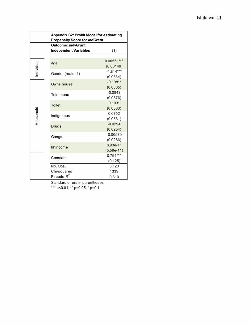
Ishikawa 41  

Outcome: indvGrantIndependent Variables (1)

0.00551***(0.00149)-1.814***(0.0534)-0.198**(0.0805)-0.0843(0.0876)0.103*

(0.0583)0.0752

(0.0581)-0.0294(0.0254)-0.00570(0.0286)8.93e-11

(5.59e-11)0.794***(0.125)

No. Obs. 3,123Chi-squared 1339Pseudo-R2 0.310

Constant

Standard errors in parentheses*** p<0.01, ** p<0.05, * p<0.1

Appendix G2: Probit Model for estimating Propensity Score for indGrant

Indi

vidu

al Age

Gender (male=1)

Hou

seho

ld

Owns house

Telephone

Toilet

Indigenous

Drugs

Gangs

hhIncome

Ishikawa 42  

References

Barber, S. L., & Gertler, P. J. (2008). The impact of Mexico's conditional cash transfer

programme, Oportunidades, on birthweight. Tropical Medicine and International Health,

13(11), 1405-1414.

Barham, T. (2011). A healthier start: the effect of conditional cash transfers on neonatal and

infant mortality in rural Mexico. Journal of Development Economics, 94(1), 74-85.

Behrman, Jere R. , & Todd, Petra E. . (1999). A Report on the Sample Sizes used for the

Evaluation of the Education, Health, and Nutrition Program (PROGRESA) of Mexico

International Food Policy Research Institute.

Conway, Dennis, & Cohen, Jeffrey H. (1998). Consequences of Migration and Remittances for

Mexican Transnational Communities. Economic Geography, 74(1), 26-44. doi:

10.2307/144342

Dostie, Benoit, & Léger, Pierre Thomas. (2009). Self-Selection in Migration and Returns to

Unobservables. Journal of Population Economics, 22(4), 1005-1024. doi:

10.2307/40344766

Fiszbein, Ariel, Schady, Norbert, & Ferreira, Francisco H. G. (2009). Conditional Cash

Transfers: Reducing Present and Future Poverty. World Bank.

Grun, Rebekka E. (2009). Exit and save: migration and saving under violence: The World Bank.

Harris, John R., & Todaro, Michael P. (1970). Migration, Unemployment and Development: A

Two-Sector Analysis. The American Economic Review, 60(1), 126-142. doi:

10.2307/1807860

Ishikawa 43  

Lindstrom, David P., & Lauster, Nathanael. (2001). Local Economic Opportunity and the

Competing Risks of Internal and U.S. Migration in Zacatecas, Mexico. International

Migration Review, 35(4), 1232-1256. doi: 10.2307/3092009

Paes-Sousa, R., Santos, L. M. P., & Miazaki, É S. (2011). Effects of a conditional cash transfer

programme on child nutrition in Brazil. Bulletin of the World Health Organization, 89(7),

496-503.

Rubalcava, Luis , & Teruel, Graciela (2006). User's Guide for Mexican Family Life Survey First

Wave.

Sjaastad, Larry A. (1962). The Costs and Returns of Human Migration. Journal of Political

Economy, 70(5), 80-93. doi: 10.2307/1829105

Skoufias, Emmanuel, Davis, Benjamin, & de la Vega, Sergio. (2001). Targeting the Poor in

Mexico: An Evaluation of the Selection of Households into PROGRESA. World

Development, 29(10), 1769-1784. doi: 10.1016/S0305-750X(01)00060-2

Skoufias, Emmanuel, Parker, Susan W., Behrman, Jere R., & Pessino, Carola. (2001).

Conditional Cash Transfers and Their Impact on Child Work and Schooling: Evidence

from the PROGRESA Program in Mexico [with Comments]. Economía, 2(1), 45-96. doi:

10.2307/20065413

Stark, Oded, & Lucas, Robert E. B. (1988). Migration, Remittances, and the Family. Economic

Development and Cultural Change, 36(3{Stark, 1988 #53}), 465-481. doi:

10.2307/1153807

Stark, Oded, & Taylor, J. Edward. (1991). Migration Incentives, Migration Types: The Role of

Relative Deprivation. The Economic Journal, 101(408), 1163-1178. doi:

10.2307/2234433

Ishikawa 44  

Stecklov, Guy, Winters, Paul, Stampini, Marco, & Davis, Benjamin. (2005). Do Conditional

Cash Transfers Influence Migration? A Study Using Experimental Data from the

Mexican Progresa Program. Demography, 42(4), 769-790. doi: 10.2307/4147339

Stiglitz, Joseph E. (1974). Alternative Theories of Wage Determination and Unemployment in

LDC's: The Labor Turnover Model. The Quarterly Journal of Economics, 88(2), 194-

227. doi: 10.2307/1883069

Support to Oportunidades Project. (2013). 2014, from

http://www.worldbank.org/projects/P115067/support-oportunidades-project?lang=en

Talyor, J.E. "Differential Migration, Networks, Information and Risk,” Research in Human

Capital and Development: Migration, Human Capital and Development, 4: 147-171.

Velásquez, Andrea. (2014). The Economic Burden of Crime: Evidence from Mexico. Duke

Economics Working Paper.