Sabine Wende1,*

Thomas R. Berry-Stölzle2

Gene C. Lai3

This draft: July 2008

1 Department of Risk Management and Insurance, University of Cologne, Albertus-Magnus-Platz, 50923 Cologne, Germany, Tel.: +49-221-470-2330, Fax +49-221-428-349, sabine.wende@uni-koeln.de.

2 Terry College of Business, University of Georgia, 206 Brooks Hall, Athens, GA 30602, Tel.: +1-706-542-5160, Fax: +1-706-542-4295, trbs@terry.uga.edu.

3 Department of Finance, Insurance, and Real Estate, Washington State University, P.O. Box 644746, Pullman, WA 99164-4746, Tel.: +1-(509)-335-7197, Fax +1-509-335-3857, genelai@wsu.edu.

* Please address all correspondence to Sabine Wende.

The Effect of Regulation on Comparative Advantages of Different Organizational Forms: Evidence from the

German Property-Liability Insurance Industry

2

1. Introduction

The relation between organizational structure and efficiency has been an important topic in

the insurance literature (e.g. Weiss, 1991; Cummins, Weiss, Zi, 1999). Agency theory has led to

the development of several hypotheses about organizational forms, resulting from the observation

that stock companies and mutual companies have comparative advantages in dealing with differ-

ent types of agency costs (Jensen and Meckling (1976), Mayers and Smith (1981) and Fama and

Jensen (1983)).

Demsetz and Lehn (1985) suggest that regulation “provides some subsidized monitoring and

disciplining of the management of regulated firms.”1 We modify Demesetz and Lehn (1985) and

argue that the regulatory environment restricts the way insurance companies can conduct busi-

ness, hence, influences the goals of the owners, managers and policyholders of these companies.

We extend the literature and suggest that the comparative advantages of different organizational

forms depend on the regulatory environment.

The goals of this paper are two folds. First, we examine the relation between efficiency and

organizational structure in the German insurance industry. Second, we investigate the effect of

the regulatory framework on the relative efficiency of alternative organizational forms in the in-

surance industry. We test our hypothesis using the data from the German property-liability insur-

ance industry.

The reasons we choose the German property-liability insurance industry as our sample are

stated below. First, the German property-liability insurance industry is different from the U.S. in

that there exists one special type of organizational form, public insurance companies, in the Ger-

man property-liability insurance industry. More important, pubic insurers were founded as non-

profit organizations with the purpose to serve a certain region or administrative district and were

equipped with monopoly authorization for a compulsory business line for their district before

1994. We hypothesize that public insurers are more cost efficient then stock insurers if they have

monopoly authorization for a compulsory business line. We refer to this hypothesis as the com-

pulsory monopoly hypothesis.

Second, the German insurance market went through a major change in the regulatory envi-

ronment. Specifically, the deregulation of the German insurance market on July 29, 1994

changed the regulatory regime dramatically, while the market and other institutional details have

1 Demstz and Lehn (1985) forcus their discussions on the relation between the regulation and ownship concentra-tion.

3

remained relatively stable. This natural experiment allows us to analyze the efficiency of insur-

ance companies with different organizational forms in the pre- and post-deregulation period sepa-

rately.

Third, it should be noted that the regulatory regime restricts competition (such as uniform

product) and especially provides disincentives to minimize costs before 1994. We extend the lit-

erature and suggest that the comparative advantages of different organizational forms depend on

the regulatory environment. We refer this hypothesis as the regulatory hypothesis.

Our analysis provides four main results: First, our results are consistent with our hypotheses

that regulation influences comparative advantages of organizational forms. Specifically, we find

that the stock cost frontier does not dominate the cost frontiers of the other organizational forms

during the regulated period when regulation was very strict. This result is consistent with the

regulatory hypothesis. More important, we find that the public cost frontier dominates the stock

cost frontier for this time period. This result is striking because it is not consistent with the ex-

pense preference hypothesis. The finding is consistent with the compulsory monopoly hypothesis.

We attribute these findings to the monopoly of public insurers in the compulsory building insur-

ance line which existed until July, 1994 because of regulation.

Second, consistent with the expense preference hypothesis, the stock cost frontier dominates

the public cost frontier after the deregulation. In other words, the expense preference hypothesis

is supported by our evidence after the deregulation for the relation between stock and public in-

surers. The first two results imply that the regulation plays an important role for efficiency.

Other findings are stated below. First, stock, mutual and public insurers are operating on

separate production hence represent different technologies. Second, the stock technology domi-

nates the mutual technology for producing stock outputs and the mutual technology dominates

the stock technology for producing mutual outputs. The same relationship holds for the stock

technology and the public technology. These findings support the efficient structure hypothesis.

In addition, we contribute to the literature on alternative organizational forms by including

publicly owned insurance companies in our analysis.

This paper proceeds as follows. In the next section we describe the German Insurance mar-

ket and its regulation. Section 3 develops hypotheses. We discuss data and methodology in sec-

tion 4. Section 5 shows the results. The final section concludes.

4

2. The German Insurance Market and its Regulation

The German insurance market is the fifth largest, in terms of premium revenue, of all insur-

ance markets in the world and the third largest in Europe. The German property-liability insur-

ance market is the largest in Europe and the second largest worldwide. The insurance sector in

Germany represents 6.8 percent of the country’s total GDP in 2006 (Europe: 9.0 percent). As in

the United States, most insurers are organized as stock companies (75 percent) or mutual associa-

tions (20 percent). However, there is a third organizational form in Germany, namely public in-

surance companies (5 percent). These insurers are created by a public decree, are subject to pub-

lic law and serve a public purpose.

Public Insurance Companies in Germany

A specific characteristic of the German insurance market is the existence of public insurance

companies as a third organizational form besides stock insurers and mutual insurers. The devel-

opment of the German insurance industry dates back to the 16th century when the first private

forms of fire insurance carriers were established. Since the availability of fire insurance was seen

as an important public good, various German states set up numerous public fire insurance com-

panies during the 18th century. These insurers were founded as non-profit organizations with the

purpose to serve a certain region or administrative district and were equipped with monopoly

authorization to offer fire insurance coverage for buildings in their district. Furthermore, in re-

gions served by a public insurance company, it was usually compulsory for owners of buildings

to purchase fire insurance coverage from these companies. The monopoly authorization of public

insurance companies as well as the legal obligation to insure buildings was later extended to in-

clude additional perils like earthquake, flood, avalanche and volcanic eruption. Even though the

monopoly authorization of public insurance companies, the legal obligations to insure buildings

with these companies, as well as the tie of public insurers to a certain administrative district were

abolished together with the deregulation of the German insurance market in 1994. Most public

insurers still restrict their business to “their” region till this date. Because public insurers have the

goal to serve their policyholders, they were not subject to regulatory supervision until after World

War II.

At the beginning of the 20th century, public insurers started to extend their business to other

lines of property-liability insurance as well as life insurance and competed with private insurers.

Foundations of public life insurance companies were usually the result of alliances between states

5

and municipal saving banks. Until today, public insurers take their mandate to serve the public

very seriously and play an important role in providing local employment opportunities and in the

promotion of arts, sciences, sports and social activities.

An important characteristic of public insurance companies is that they are now all owned by

municipals savings banks (Sparkassen) and their associations (Sparkassenverbänden). After the

monopoly authorization of public insurers fell together with the deregulation of the German in-

surance market, the German states sold their shares in the public insurance companies to the mu-

nicipal savings banks. The motivation for these transactions was that an alliance with the group

of the municipal savings banks will help public insurers to compete in a deregulated insurance

market.

Municipal savings banks in Germany are non-profit savings and loan banks set up under

public law with the purpose to serve a certain region or administrative district. All municipal sav-

ings banks are organized in associations which are themselves members of one umbrella associa-

tion (Deutscher Sparkassen und Giroverband). These associations provide services to all member

savings banks like joint marketing activities and consulting services. Municipal savings banks in

Germany have their own deposit guarantee scheme which is based on a joint liability with respect

to deposits. Therefore, the group of municipal savings banks can be viewed as a decentralized

financial conglomerate under public law, and this conglomerate now also includes investment

companies, home savings and loan associations, leasing companies, factoring companies as well

as all twelve public insurance companies. Municipal savings banks are one of the major providers

of corporate loans and mortgages. These loans and mortgages usually have an insurance require-

ment on the property used as security resulting in substantial cross-selling opportunities for in-

surance products.

During the regulated era, public insurers had monopoly authorization for policies covering

direct damage to building structures through fire and other perils. Under deregulation, policies

covering direct damage to building structures as well as similar products such as homeowner’s

personal property coverage are well suited for cross-selling because they can be bundled easily

with the loan or mortgage.

6

Insurance Regulation before July 1994

The establishment of a federal regulatory authority2 in Germany dates back to 1901 when

the federal regulatory law went into force.3 The German regulatory law is based on the principal

that insurance regulation has to protect the interests of the insured, hence, requires prior approval

of insurance contract terms by the Federal Insurance Authority. The Insurance Authority had

considerable discretion in the approval of contract terms and took the position that insurance con-

tracts should be uniform across insurance companies. The so called “principal of uniformity”

results from the point of view that market transparency is a necessary condition to ensure the in-

terests of the insured. The crucial philosophical assumptions underlying the argument are that

first, an ordinary consumer is not capable of comparing different insurance contracts and making

a rational buying decision. Second, insurance regulation has to protect consumers from buying

inadequate insurance coverage. Therefore, all insurance products should have a minimum quality

and as little variation in contract terms as possible. In such a “transparent market” consumers can

rely on the quality of the products, and only have to compare the prices. To achieve uniformity,

the Insurance Authority declares certain contracts as standard. Contract terms deviating from the

standard do not have a chance of getting approval unless the Insurance Authority believes this

deviation stands for real progress (Angerer, 1985). It is a corollary of this line of thought that new

contracts deviating from the standard should not be approved for individual insurers. Rather, the

standard itself should be revised and improved. Approval of the standard contract terms for use

by individual insurers is only a matter of routine because the Insurance Authority usually pub-

lishes approved contract terms (Eggerstedt, 1987). This provides a strong incentive to use stan-

dard contract terms because it is not possible to gain a competitive advantage through the devel-

opment of a new product.

All German insurers belong to associations that are organized according to the types of in-

surance business. These associations play an important role in the pricing of insurance coverage.

They collect loss data from their members and generate aggregated statistics. But they also calcu-

late rates which are based on these aggregated statistics, and recommend these rates to be used by

their members. Such rate recommendations are possible because §102 of the German Cartel Law

exempts insurers from most antitrust regulation.

2 Kaiserliches Aufsichtsamt für Privatversicherung, later named Reichsaufsichtsamt für Privatversicherung. After World War II the occupation forces created supervisory agencies. In 1951 the new Bundesaufsichtsamt für das Versicherungswesen (BAV) was established. Since many staff members of the old Reichsaufsichtsamt worked for the British Zone agency, and the BAV took over most of their staff, there was some continuity in regulation (Kimball and Pfennigstorf, 1965). 3 Reichsgesetzt über die private Versicherungsunternehmung, May 12, 1901, in: Reichsgesetzblatt 139. Today’s Gesetz über die Beaufsichtigung der Versicherungsunternehmen (or Versicherungsaufsichtsgesetz) is based on this law with only modest changes.

7

In summary, in personal lines, which accounted for over 70% of the overall premiums writ-

ten in 1990, there was almost no product competition. In fact, the environment in personal lines

provided strong incentives for collusion in pricing. The situation in large commercial lines was

less restrictive, but these lines did account for less than 30% of the market. Overall, the behaviour

of German insurance companies before the deregulation can be described as a convoy led by the

Insurance Authority and the associations (Farny, 1999). Therefore, management activity focused

on the distribution system, marketing activity, customer service, and the improvement of business

processes rather than on cost reduction.

Deregulation of the Insurance Industry

The deregulation of the German insurance industry is a result of the creation of the European

Single Market. Since the founding of the European Community (EC) in 1957, its member states

had been working on the creation of an integrated economic market. The framework for a single

European insurance market was finally completed in July 1994. The accompanying harmoniza-

tion of regulatory systems was designed to create a level playing field for all insurance companies

within the European Union (EU).

The most profound regulatory change came in 1994. Since then, insurance companies only

need a single license from their state of origin to write all types of insurance business in all mem-

ber states of the EU, and they are only subject to regulation in their state of origin. Since the in-

surance contract law and the tax law of the host country still apply, insurers have to develop dif-

ferent products for different countries, making cross-border services difficult. Thus, the market

share of cross-border business from European insurers in Germany is negligible. It was only

0.9% in 2003.4 Even the market share of European insurers establishing branches in Germany is

very small (1.5% in 2003) indicating that the creation of the European single market did not in-

crease the competition significantly. But two side effect of the single market, the requirement that

all member states abolished prior approval of insurance contract terms and rates as well as all

monopoly authorizations, changed the German insurance market dramatically. These changes can

be tied to July 29, 1994, the date when the legislation incorporating the third non-life insurance

directive into German law went into effect. The deregulation of insurance contract terms and

rates resulted in product and price competition among the insurers licensed in Germany and oper-

4 Data on market shares is from the 2005 yearbook of the insurance supervisory authority (BaFin).

8

ating under the German regulatory regime. For public insurance companies, the fall of their mo-

nopoly authorization further increased the competitive pressure.

Effects of the German Reunification on the Insurance Industry

In addition to the deregulation of the German insurance market on July 29, 1994, the Ger-

man Reunification on October 3, 1990 also changed the operating environment for German in-

surance companies. In the former German Democratic Republic there was a strong social security

system but hardly any private insurance. The Staatliche Versicherung der DDR was the only in-

surance company in operation. This insurance company offered a wide variety of products rang-

ing from homeowners, liability, life, accident and auto insurance to health insurance for self-

employed professionals. However, most individuals relied more on the social security system

then on private insurance solutions, and the ones who purchased private insurance had relatively

low policy limits as measured by West German standards.5

As the five reestablished states of East Germany - Brandenburg, Mecklenburg-

Vorpommern, Saxony, Saxony-Anhalt and Thuringia - formally joined the Federal Republic of

Germany on October 3, 1990 all insurance companies licensed in West Germany could also offer

their products in these new states. In the years 1991-1994 the German insurance market was still

heavily regulated, hence, the German Reunification basically increased the market for the stan-

dardized German insurance products over night which resulted in tremendous growth for the in-

surance industry.

3. Hypothesis Development

The following section states our hypotheses about the relationship between the organiza-

tional form of insurance companies and their efficiency. Our analysis focuses explicitly on the

mediating effect insurance regulation has on this relationship. Existing theoretical and empirical

research on organizational forms assumes a competitive market environment. We extend this

literature developing a framework that explains the relative advantage one organizational form

has over another in a strictly regulated insurance market.

5 After the Reunification, the largest German insurance company, the Allianz AG, bought the insurance portfolio of the Staatliche Versicherung der DDR.

9

H1: Regulatory Hypothesis

Regulation has a mediating effect on the relationship between the organizational structure

of an insurance company and its efficiency.

Demsetz and Lehn (1985) suggest that regulation “provides some subsidized monitoring and

disciplining of the management of regulated firms.”6 We modify Demsetz and Lehn (1985) and

argue that the regulatory environment restricts the way insurance companies can conduct busi-

ness, hence, influences the goals of the owners, managers and policyholders of these companies.

We extend the literature and suggest that the comparative advantages of different organizational

forms depend on the regulatory environment.

H2a: Expense Preference Hypothesis A

In a competitive market environment, mutual insurers are less successful in minimizing

costs than stock insurers because of the unresolved agency conflicts.

We extend the well known expense preference hypothesis, to public insurance companies.

Because the mutual form does not provide powerful mechanisms to control the owner-manager

conflict, manager can get away with the consumption of perquisites increasing the company’s

expenses. Public insurance companies on the other hand are founded as non-profit organizations

with the purpose to serve a certain region or administrative district. This goal may conflict with

the economic goal to minimize costs in the production of insurance coverage from time to time.

Boycko, Shleifer and Vishny (1996), for example, argue that due to the influence of politicians,

public firms employ excess labor.

H2b: Expense Preference Hypothesis B

In a competitive market environment, public insurers are less successful in minimizing

costs than stock insurers because of their objective to serve a region.

H2c: Expense Preference Hypothesis C

In a strictly regulated market environment without incentives for cost minimization, stock

insurance companies are not more successful in minimizing costs than any other organiza-

tional form.

6 Demsetz and Lehn (1985) focus their discussions on the relation between the regulation and ownership concentra-tion.

10

The literature has applied the DEA to examine the organizational structure and efficiency.

Cummins et al. (2004) propose the efficient structure hypothesis and state that different organiza-

tional forms are sorted into market segments where they have comparative advantages in agency

and production costs. This argument does not only apply to stock and mutual insurance compa-

nies but also to public insurers. Hence:

H3a: Efficient Structure Hypothesis A

In a competitive market environment, stock, mutual and public insurers are sorted into

market segments where they have comparative advantages in agency and production

costs.

Since the basic economic principle that corporations or individuals divide labor based on

their competencies applies to strictly regulated markets as well, we argue that the efficient struc-

ture hypothesis is valid unaltered in a regulated insurance market as well. Hence:

H3b: Efficient Structure Hypothesis B

In a strictly regulated market environment, stock, mutual and public insurers are sorted

into market segments where they have comparative advantages in agency and production

costs.

Because the stock ownership form makes it possible for owners to control managers effec-

tively, stock insurers have comparative advantages in lines of insurance business where high

level of managerial discretion is required. Mayers and Smith (1988) refer to this argument as the

managerial discretion hypothesis. In addition, the maturity hypothesis states that mutual compa-

nies are relatively successful in business lines with lengthy claim settlement lags, because the

owners’ incentive to exploit policyholder interests is removed by merging the owner and policy-

holder function. However, insurance regulation might limit the degree of discretion managers

have quite substantially. Hence:

H4a: Managerial Discretion Hypothesis A

In a competitive market environment, stock insurers have comparative advantages in

short-tail lines of business where a high level of managerial discretion is required.

11

H4b: Managerial Discretion Hypothesis B

If insurance regulation restricts managerial discretion, stock insurers do not have com-

parative advantages in short-tail lines of business where a high level of managerial discre-

tion is required.

Public insurers in Germany were founded as non-profit organizations with the purpose to

serve a certain region or administrative district and were equipped with monopoly authorization

in the compulsory building insurance line for their district. However, they also offered other in-

surance products we hypothesize that public insurers have comparative advantages in the com-

pulsory business line in a regulated environment. We refer to this hypothesis as the compulsory

monopoly hypothesis. Hence:

H5: Compulsory Monopoly Hypothesis

If public insurance companies have monopoly authorization for a compulsory business

line, they have a comparative advantage in this business line.

After the deregulation of the German insurance market the German states sold their shares in

the public insurers to the municipal savings banks. Since municipal savings banks are one of the

major providers of corporate loans and mortgages in Germany, public insurers should benefit

from this alliance by selling products in lines with relations to the banking business. Specifically,

we expect that policies covering direct damage to building structures as well as similar products

such as homeowner’s personal property coverage are well suited for cross-selling because they

can be bundled easily with a loan or mortgage. Hence:

H6: Public financial conglomerate hypothesis

If public insurance companies and municipal savings banks form a financial conglomerate

public insurers have a comparative advantage in lines with relations to the banking busi-

ness.

12

4. Data and Methodology

4.1 Data

In our assessment of the German insurers, we use company level data of property-liability

insurance companies supervised by the German insurance authority (BaFin). We restrict our

analysis to insurance companies which have gross premiums written of at least 50 million Euros

per year for the years 1988-2005. The data for the insurers in our sample is obtained from their

annual reports. There are 40 insurance companies in our sample, and these insurance companies

account for an average of 55% of the overall written premium volume of the German property-

liability insurance market. The final sample includes 26 stock, 8 mutual, and 6 public insurers in

each year of the sample period. Thus, we have 720 firm observations over the whole sample pe-

riod.

Table 1 presents yearly growth rates of premiums written, total invested assets, losses in-

curred and total assets for the insurance companies in our sample. All growth rates are signifi-

cantly higher for the 1991 through 1994 period than for the time periods before 1991 and after

1994. In October 1990 the German Reunification occurred and in July 1994 the German insur-

ance market was deregulated. Thus, in the years between these two events, the German insurance

market was still heavily regulated, but experienced tremendous growth.

[Table 1: Yearly Growth Rates of Selected Variables]

Table 2 presents yearly premium growth rates for the three organizational forms: stock in-

surers, mutual insurers and public insurers. For the years 1991 through 1994, premium growth

varies substantially across organizational forms; growth rates are highest for stock insurers and

lowest for public insurers.

[Table 2: Differences in Premium Growth Rates across Organizational Forms]

Overall, these results indicate that the German Reunification had a substantial impact on the

German insurance industry. It is therefore important to control for this effect in our analysis how

regulation affects the comparative advantages of different organizational forms. To address this

issue, we analyze the three time periods before 1991, 1991 through 1994 and after 1994, sepa-

rately, and carefully interpret the results.

13

4.2 Methodology

In our analysis we follow the non-parametric Data Envelopment Analysis (DEA) approach

of Cummins, Weiss and Zi (1999). This approach based on the work of Farrell (1957) and Fähe,

Grosskopf, and Lovell (1985). More precisely, we apply the input oriented DEA and differentiate

between the technical efficiency (TE), the allocative efficiency (AE), and the cost efficiency (CE)

of each firm. While TE expresses the effectiveness with which a given set of inputs is used to

produce a maximum output, AE expresses the effectiveness of the allocation of inputs given the

prices of the inputs. CE reflects the combination of TE and AE, which means that a firm adopts

the best technology (TE) and chooses the optimal input mix (AE) (Coelli, 1996).

Technical, Allocative and Cost Efficiency

To illustrate the efficiency measurement in a simple way Figure 1 shows a production fron-

tier with two inputs (x1 and x2) and one output (y). We are using an input-oriented DEA; in this

case the isoquant SS’ characterizes the multiple combinations of the two inputs producing a fixed

output. A firm operates technical efficiently with the best available technology if it is located on

the isoquant, e.g. point Q. Technically inefficiency is presented in the input-combination of point

P. The ratio QP/0P symbolizes the percentage of input reduction of one firm if this firm adopts

the best technology. The TE is characterizes by

TE = 0Q/0P,

which is the inversion of 1 minus QP/0P. The value of the TE ranges from zero to one. One indi-

cates fully efficiency.

[Figure 1: Technical Efficiency]

The ratio of input prices is presented by the isocost line AA’ shown in Figure 1. A firm op-

erates allocative efficiently with the optimal input mix if it is located on the isocost line, e.g.

point R. So AE is represented by the ratio

AE = 0R/0Q.

The optimal operating point is represented in point Q’, where the isoquant is tangent the iso-

cost line. On this point the operating firm is fully cost efficient. CE is defined as the ratio:

CE = 0R/0P.

14

Cost Efficiency is then defined as the product of TE and AE:

Cost Efficiency = Technical Efficiency × Allocative Efficiency

or

0R/0P = (0Q/0P) × (0R/0Q). (1)

Cost efficiency is estimated by solving linear programming problems. The first step is to

calculate the minimum cost, MC, of producing the output of a particular firm. Specifically, for

the multiple input–output situations the following LP problem is solved:

Minimize: *ipx

Yyi

Subject to: Xxi

. R (2)

In this problem, y is the m-dimensional vector of output produced by a particular firm; xi is

the n-dimensional vector of inputs used by a particular firm; Y is the (k × m) matrix of outputs

where k represents the number of firms; X is the (k × n) matrix of inputs; λ is a (m × 1) vector of

intensity parameters or weights attached to each observations in the determination of minimum

cost; and p is the n-dimensional vector of input prices. The input values generated by the solution

to the above problem *ix represent the minimum cost vector of input for the i-th firm. The total

CE of i-th firm would then be calculated as:

,/*ii pxpxCE

which is the ratio of minimum cost to observed cost. This ratio corresponds to 0R/0P in Figure 1.

A measure of TE is also developed using a second LP problem. The LP problem is stated as:

In this problem, TE is a scalar with all of the other symbols as defined previously. For instance,

in Figure 1 TE of point P responds to 0Q/0P. After TE and CE are calculated, AE is derived

through Equation (1) as AE = CE/TE.

Minimize: TE

Yyi

Subject to: XxTE i *

. R (3)

15

Cross-Frontier Distance Function

In this section, we review an approach called “cross-frontier efficiency method” which was

advanced by Cummins et al. (1999) comparing mutual and stock insurers. Through the estimation

of cross-frontier distance function, this approach allows us to compute the efficiency of the firms

in each ownership group with reference to the other group’s production or cost frontier. The pur-

pose of this approach is to help us examine whether each group’s output vector could be pro-

duced with equal efficiency using the other group’s technology.

We begin our discussion of cross-frontier distance function with the introduction of input-

oriented distance function (Shephard, 1970). To illustrate the distance function, consider the firm

operating at point (xm,ym) in Figure 2. Although xm represents input of the mutual firm m, ym

represents the output of the firm m in period t, and Vm and Vs are the frontiers of mutual firm m

and stock firm s, respectively. Subscripts on D in the following distance functions indicate the

reference set of firms used to construct the frontier. For example, Dm(xm,ym) denotes the produc-

tion point (xm,ym) with respect to the mutual frontier Vm. The distance function value for this firm

relative to the mutual frontier is given by Dm(xm,ym) = 0e/0d. One can see that the measure of

Farrell’s TEm of point (xm,ym) = 0d/0e, which happens to be the reciprocal of the input distance

function of the specific point. Although TE of a production point is always ≥ 1, input distance

function value is always ≤ 1.

However, input distance function “relative to the other group’s function” is not necessarily

always ≥ 1. This is the so-called “cross-frontier” distance function, and we illustrate it using the

example of input distance function of a mutual firm (xm,ym) relative to the stock frontier Vs,

Ds(xm, ym) in Figure 2. For the specific production point (xm,ym), the distance value with respect

to the stock frontier Vs is 0d/0c, which is smaller than 1 as the stock frontier lies to the right of the

point. It implies that this mutual firm has a technological advantage in producing in its output

range. If the whole mutual group performs in the same way, it means the mutual firms are domi-

nant in producing their outputs using their own technologies.

[Figure 2: Stock and Mutual Frontier]

Cross-to-Own Frontier Analysis

The measurement of the distance between the frontiers is possible at each operating point

(see Figure 2). It is also probable to decompose a firm’s group-specific frontier distance into:

distance between frontiers × distance from the frontier relevant to the other group of firms. We

16

follow Cummins et al. 2004 and use the notation DT{M:S}(xm,ym) to illustrate the distance between

the production frontiers (symbolized by subscript T) with respect to the mutual firm’s operating

point (xm,ym), for stock insurers vice versa. We compute the mutual firm’s distance function

value relative to the mutual frontier:

Dm(xm,ym) = DT{M:S}(xm,ym) × Ds(xm,ym) = 0e0c/0d0d × 0d/0c = 0e/0d (4)

This permits us to estimate the distance between the mutual and the stock frontier for each

operating point by the product of the ratio of the own-frontier distance function to the cross-

frontier distance function, i.e. DT{M:S}(xm,ym) = Dm(xm,ym) / Ds(xm,ym). This projects each firm’s

operating point to its own-frontier.

By using Farrells technical efficiency as the reciprocal of the distance function value, the

cross-frontier can be expressed as the ratio of the cross-frontier technical efficiency to the own-

group (own-frontier) technical efficiency: DT{M:S}(xm,ym) = Ts(xm,ym) / Tm(xm,ym) for mutual

firms, and DT{S:M}(xs,ys) = Tm(xs,ys) / Ts(xs,ys) for stock insurers. On this account, we refer D-

T{M:S}(xm,ym) and DT{S:M}(xs,ys) as the cross-to-own-efficiency ratios. For allocative and cost effi-

ciency analogous ratios are achieved. If that firm’s group-specific frontier dominates the other

group’s frontier the distance between the frontiers for any given operating point is > 1 and < 1 if

the other group’s frontier dominates the firm’s group-specific frontier.

Measuring Inputs, Outputs and Prices

Consistent to the recent insurance and banking literature, we adopt the well established

value-added approach to measure property-liability insurers’ outputs and inputs (Berger and

Humphrey, 1992; Yuengert, 1993; Cummins, Tennyson, and Weiss, 1999).7 For the DEA we

used two outputs and three inputs.

Outputs

We select the present value of claims incurred net of reinsurance as one output variable. We

also select total invested assets as a second output. Both outputs are deflated to the base year

2000 using the German Consumer Price Index (CPI).

Inputs

We classify insurance inputs into three different groups: labor and business services, equity

capital, and dept capital. The operating expenses express the labor and business service compo-

7 We did not use the financial intermediate approach for the reason that it is not appropriate for the property-liability insures because their services are not limited to financial intermediation, see Cummins, Weiss, Zi, 1999; Lai, Jeng, 2005.

17

nent including commissions and salaries. The input price is the average expense for insurance

business services including average wages for commissions and salaries.

The second input factor is equity capital. Equity capital is measured by book value. As a

second price measure we adopt the dept-equity ratio of the firm following Jeng, Lai, McNamara,

2007.

The final input is dept capital proxied by technical provisions net of reinsurance. The three

years German Treasury Bills is the deflated input price for dept capital.

5. Results

5.1 Descriptive Statistics for Inputs, Outputs and Prices

Table 3 provides descriptive statistics for inputs, outputs and input prices for all insurers and

the sub-samples of the three organizational forms: stock, mutual, and public insurers. Overall, the

mean values for most variables are higher for stock insurance companies than for mutual and

public insurers. The mean for the equity capital variable, however, is smaller for stock insurers

than for mutual and public insurers. There are two possible explanations for this result. First, the

stock insurers in our dataset write more business in short-tail lines than mutual and public insur-

ers. Since losses in short-tail lines are ceteris paribus better predictable than losses in long-tail

lines, stock insurers should on average hold less capital than mutual and publics insurers. Second,

stock insurers have access to the capital market if their capital gets depleted. This option reduces

their need to hold capital within the company.

[Table 3: Descriptive Statistics for Output and Input Variables]

5.2 Cross Efficiency Results

We follow the procedure of Cummins, Weiss and Zi (1999) and first test whether the three

organizational forms have different production technologies. Comparing the insurance compa-

nies’ efficiency scores based on the pooled efficiency frontier with efficiency scores based on

group specific frontiers, we find significant differences of the group means for both, technical

efficiency (TE) and cost efficiency (CE). These results indicate that the separated frontiers are

significantly different from the pooled frontier. Thus, we can conclude that the pooled methodol-

ogy is not appropriate for our dataset because stock, mutual and public insurers use different

technologies and operate on different production frontiers.

18

We next analyse the cross frontier efficiencies, results are presented in Tables 4 and 5. We

compute technical efficiency of the stock relative to the mutual frontier Tm(xs,ys) and relative to

the public frontier Tp(xs,ys). We also conduct the same analysis for cost efficiency. Finally, we

examine mutual and public efficiency relative to the other two frontiers. If the cross frontier re-

sults are greater than 1, this implies that it is not feasible to replicate one firms input-output com-

bination using the other firms technology for producing the first firms output.

Table 4 shows the technical efficiency scores for the years 1988 through 2005. Let us first

focus on the results for the 1988 through 1990 period. For all three years the mutual technical

efficiency on the stock frontier Ts(xm,ym) is greater than one and the stock technical efficiency on

the mutual frontier Tm(xs,ys) is greater than one as well. This implies that mutual insurers and

stock insurers have developed dominant technologies and, hence stock (mutual) insurers are not

able to produce the mutual (stock) insurer’s output vector with equal efficiency. When comparing

stock insurers with public insurers for the 1988 through 1990 time period, we find the same re-

sult; both organizational forms have a dominant technology to efficiently produce their own out-

put vector. The comparison between the mutual insurers and the public insurers is not as clear.

The mutual technical efficiency on the public frontier Tp(xm,ym) is greater than one for all three

years, but the public technical efficiency on the mutual frontier Tm(xp,yp) is smaller than one.

However, these values are relatively close to one – the smallest value is 0.97 – and, furthermore,

the public efficiency score results relative to the mutual frontier are not significantly different

from the corresponding efficiency score results relative to the public frontier. Therefore, we argue

that there is no evidence for a dominance of the mutual production technology over the public

technology. Overall the pair wise comparisons of the stock, mutual and public technical efficien-

cies provide support for the efficient structure hypothesis (H3b). All three organizational forms

focus on market segments where they have a comparative advantage.

[Table 4: Technical Efficiency Score Results of Stock, Mutual and Public Insurers

Input-Output-Combinations]

Let us now focus on the 1991 through 1994 time period. When comparing stock insurers

with mutual insurers, we find that both organisational forms have developed dominant technolo-

gies and, hence, stock (mutual) insurers are not able to produce the mutual (stock) insurer’s out-

put vector with equal efficiency. The comparisons of stock insurers with public insurers and the

19

comparison of mutual insurers with public insurers, however, provide a different result. For the

years 1992 through 1994, the stock technology can produce the public output more efficiently

than the public insurers’ own technology and this result is significant at the one percent level in

1993. Similarly, for the years 1991 through 1994, the mutual technology can produce the public

output more efficiently than the public insurers’ own technology and this result is significant in

three out of the four years. Thus, the public technology is inferior to the stock and mutual tech-

nology in the 1991 through 1994 period which can be characterized by tremendous growth op-

portunities in the territory of the former GDR after the German Reunification.

Let us now focus on the technical efficiency results for the time period after the deregulation

of the German insurance market. When comparing stock insurers with mutual insurers for the

years 1995 through 2005, we find that both organizational forms have a dominant technology to

efficiently produce their own output vector, and it is not feasible for the other organizational

form, on average, to replicate this output vector. Except for the years 1995 and 1998, we find the

same result for the comparison between the stock and the public technology. Both, stocks and

publics have a dominant technology for producing their own output vector and are, hence, effi-

cient in their market segment. When comparing the mutual and the public technology for the

years 1998 through 2005, we also find that both organizational forms efficiently produce their

own output vector, and it is not feasible for the other organizational form, on average, to replicate

this output vector. We attribute the fact that the mutual technology can produce the public output

more efficiently than the public insurers’ own technology in the years 1995 through 1997 to the

German Reunification. Since public insurance companies were restricted to a certain region be-

fore the deregulation in 1994, they could not profit from the growth opportunities of the 1991

through 1994 time period. We now argue that it took them until 1998 to finally compensate this

comparative disadvantage and re-establish their dominance in producing their output vector.

Therefore, the findings for the 1995 through 2005 period support the efficient structure hypothe-

sis (H3b).

Table 5 presents the cost efficiency scores for the years 1988 through 2005. Let us first fo-

cus on the results for the 1988 through 1990 period. Stock insurers are significantly less cost effi-

cient and are, hence, dominated by mutual insurers in producing stock output as well as produc-

ing mutual output. In addition, stock insurers are less cost efficient and are dominated by public

insurers in producing stock output and public output. These findings support the version of the

expense preference hypothesis (H2c) for regulated markets. In an environment without incentives

20

for cost minimization, stock insurers cannot use their strong mechanism to control the owner-

manager conflict for creating a comparative advantage.

[Table 5: Cost Efficiency Score Results of Stock, Mutual and Public Insurers Input-Output-

Combinations]

The time period after the German Reunification provides a different picture. For the years

1993 and 1994, it can be seen that stock insurers are more cost efficient compared to mutual in-

surers for producing stock as well as mutual input-output-combinations. Furthermore, stock in-

surers are more cost efficient and dominated public insurers in producing stock output as well as

producing public output. We attribute the improved cost efficiency of stock insurers relative to

the other two organizational forms to the faster growth of stock insurance companies after the

Reunification.

Let us now focus on the cost efficiency results for the time period after the deregulation of

the German insurance market. When comparing stock and mutual insurers, stock insurers are

only more cost efficient in producing stock as well as mutual outputs for the four years 1998

through 2001. For the periods 1995 through 1997 and 2002 through 2005, stock insurers are more

cost efficient in producing stock outputs, but mutual insurers are more cost efficient in producing

mutual outputs. In addition, it is not feasible for stock insurers, on average, to replicate the mu-

tual output vector for the years 2002 through 2005. Therefore, we conclude that our results do not

support the expense preference hypothesis A (H2a). The comparison between stock and public

insurance companies, however, supports the expense preference hypothesis B (H2b). Specifically,

stock insurers are more cost efficient and dominate public insurers in producing stock output as

well as producing public output.

5.3 Regression Results

To analyze the comparative advantages of the stock, mutual and public ownership forms by

lines of business, we perform a regression analysis of the cross-to-own efficiency ratios for tech-

nical and cost efficiency. More precisely, for each pair of the three ownership forms, we regress

the cross-to-own efficiency ratios on a set of independent variables representing the organiza-

tional form, size, business mix, and year fixed effects. Organizational form is captured by two

dummy variables: The stock variable is coded as 1 for stock insurers and 0 otherwise, and the

mutual variable is coded as 1 for mutual insurers and 0 otherwise. We include three size quartile

21

dummy variables in the regression; the omitted first quartile is the smallest. The variable LT%

represents the percentage of gross premiums written in long-tail lines, and the variable BT%

represents the percentage of gross premiums written in business lines covering direct damage to

building structures as well as similar products such as homeowner’s personal property coverage.

Interaction terms between the organizational form dummy variables and the business mix vari-

ables are also included in the models to allow the effects of organizational form to differ by line.

Table 6 presents the regression results for the 1988 through 1990 time period. The first two

regressions compare the stock and mutual ownership forms. The comparative advantage of the

two ownership forms by line of business is measured directly by the coefficient for the LT% *

stock interaction term. This coefficient is positive and significant in both, the technical and the

cost regression imply that stocks tend to have a comparative advantage in writing long-tail lines

relative to short-tail lines, i.e., an increase in the fraction of business in long-tail lines tends to

shift the stock frontier to the left of the mutual frontier (see Figure 2). This result contradicts the

agency-theoretic argument that mutual insurers should have a comparative advantage in lines

with longer claim settlement periods because a longer time period gives mutual managers more

opportunities to exploit policyholder interests. But this finding is consistent with the view that a

strict regulatory environment limits managerial discretion and specifically prevents stock manag-

ers from exploiting policyholder interests. Hence, the elimination of the owner-policyholder con-

flict should not give mutual insurers a comparative advantage over stock insurers in long-tail

lines. Therefore, the positive and significant coefficient of the LT% * stock interaction term sup-

ports our managerial discretion hypothesis B (H4b).

[Table 6: Frontier Distance Regressions for the Years 1988 through 1990]

The second set of regressions in Table 6 compares the stock and public ownership forms. In

both the technical and cost regressions including the LT% variable, the coefficient of the LT% *

stock interaction term is positive and not significant. This result is consistent with the managerial

discretion hypothesis B (H4b) which predicts that a strict regulatory environment prevents stock

managers from exploiting policyholder interests in long-term lines. Hence, the reduction of the

owner-policyholder conflict should not give public insurers a comparative advantage over stock

insurers in long-term lines. In the regression model with the BT% variable, the coefficient of the

BT% * stock interaction term is negative and significant. This indicates that stocks tend to have a

22

comparative disadvantage or publics tend to have a comparative advantage in writing business

lines covering direct damage to building structures as well as similar products such as home-

owner’s personal property coverage. Since insurance coverage for buildings was compulsory

during the 1988 through 1990 time period and public insurers had monopoly authorization for

these products, the results for both the technical and cost regression support the compulsory mo-

nopoly hypothesis (H5).

The third set of regressions in Table 6 compares the mutual and public ownership form. In

the technical efficiency regression with the BT% variable, the coefficient of the BT% * mutual

interaction term is negative and significant. This result indicates that mutual insurers tend to have

a comparative disadvantage or public insurers tend to have a comparative advantage in writing

“building” lines. Since public insurers had monopoly authorization for policies covering direct

damage to buildings, this result supports the compulsory monopoly hypothesis (H5).

Table 7 presents the regression results for the 1991 through 1994 time period. A unique

characteristic of this time period following the German Reunification is the tremendous growth

of the insurance industry. However, not all companies were able to profit from this opportunity.

Therefore, we include three additional variables into our models capturing the differences in

premium growth rates between organisational forms. For each year, the growth(i,j) variable,

(i,j) {(stock,mutual), (stock,public), (mutual,public)} measures the difference in premium

growth between the individual insurers of organizational form i and the mean growth rate of the

organizational form j. A positive and significant coefficient for this variable in our regressions

indicates that a higher premium growth improves the efficiency of one organizational form rela-

tive to the other organizational form under consideration. The cost efficiency regression compar-

ing stock with mutual insurers has a positive and significant coefficient for the

growth(stock,mutual) variable. Thus, we can conclude that the faster premium growth of stock

insurers in the years following the Reunification improved their cost efficiency relative to mutual

insurers. Similarly, the coefficient for the growth(stock,public) variable is positive and significant

in the cost efficiency regression comparing stock and public insurers. Thus, we can conclude that

the faster premium growth of stock insurers after the Reunification significantgly improved their

cost efficiency relative to public insurers. We also find that the faster growth of mutual insurers

relative to public insurers after the Reunification improved the mutual insurers’ technical effi-

ciency relative to the public benchmark; the coefficient of the growth(mutual,public) variable is

23

positive and significant in the technical efficiency regression comparing mutual and public insur-

ers.

[Table 7: Frontier Distance Regressions for the Years 1991 through 1994]

Table 8 presents the regression results for the time period after the deregulation of the Ger-

man insurance market. The first two regressions compare the stock and mutual ownership forms.

In the technical regression, the coefficient for the LT% * stock interaction term is negative and

significant indicating that stocks tend to have a comparative disadvantage or mutuals tend to have

a comparative advantage in writing long-tail lines relative to short-tail lines. This result supports

the managerial discretion hypothesis A (H4a) which predicts that mutual insurers should have a

comparative advantage in long-tail lines due to reduced agency costs. Similarly, the coefficient

for the LT% * stock interaction term is negative and significant in the technical regression com-

paring stock and public insurance companies. Thus, stocks also tend to have a comparative dis-

advantage relative to public insurers in writing long-tail lines. This result is consistent with the

argument that the owner-policyholder conflict is much stronger for stock insurers than for public

insurers established as non-profit organizations serving the insurance needs of a certain region.

However, the owner-policyholder conflict is not completely eliminated for public insurers. In the

technical efficiency regression comparing publics with mutuals, the coefficient for the LT% *

mutual interaction term is positive and significant indicating that mutual insurers have a com-

parative advantage relative to public insurers in writing long-tail business lines.

[Table 8: Frontier Distance Regressions for the Years 1995 through 2005]

With respect to the financial conglomerate hypothesis (H6), we find mixed results. On the

one hand, the coefficient for the BL% * mutual interaction term is negative and significant in the

technical regression comparing mutual and public insurers. This result indicates that public insur-

ers have a comparative advantage relative to mutual insurers in business lines with relations to

the banking business. But on the other hand, the coefficient for the BL% * stock interaction term

is positive and significant in the technical regression comparing stock and public insurers. This

positive coefficient indicates that stock insurers have a comparative advantage or public insurers

have a comparative disadvantage relative to stock insurers in these business lines with relations to

the banking business.

24

Our main hypotheses is that the regulatory regime determents the relative efficiency and

therefore the comparative advantages of different organizational forms. In a competitive market

environment stock companies are the most cost efficient ones. In a highly restrictive regulatory

regime which does not provide incentives for cost minimization, however, this should be the

other way around. Consistent to this hypothesis we find that stock insurers are less cost efficient

in the regulated environment and are dominated by mutual and public insurers. Furthermore,

agency theory predicts that mutual insurers should have a comparative advantage in lines with

longer claim settlement periods because a longer time period gives stock managers more oppor-

tunities to exploit policyholder interests. But a strict regulatory environment which limits mana-

gerial discretion should prevent stock managers from exploiting policyholder interests. Consis-

tent with this hypothesis we find that stock insurance companies do not have a comparative dis-

advantage in long-tail lines in the German insurance market before its deregulation.

6. Conclusion

This study examines the relation between efficiency and organizational structure in the in-

surance industry. In addition, we also investigate the effect of the regulatory framework on the

relative efficiency of alternative organizational forms in the insurance industry. We test our hy-

pothesis using the data from the German property-liability insurance industry.

The reasons we choose the German property-liability insurance industry as our sample are

stated below. First, the German property-liability insurance industry is different from the U.S. in

that there exists one special type of organizational form, public insurance companies, in the Ger-

man property-liability insurance industry. More important, pubic insurers were founded as non-

profit organizations with the purpose to serve a certain region or administrative district and were

equipped with monopoly authorization for a compulsory business line for their district before

1994. We hypothesize that public insurers are more cost efficient then stock insurers if they have

monopoly authorization for a compulsory business line. We refer to this hypothesis as the com-

pulsory monopoly hypothesis.

Our analysis provides two main results: First, the results are consistent with our hypotheses

that regulation influences comparative advantages of organizational forms. Specifically, we find

that the stock cost frontier does not dominate the cost frontiers of the other organizational forms

during the period when regulation was very strict. More important, we find that the public cost

frontier dominates the stock cost frontier for this time period. This result is striking because it is

25

not consistent with the expenses preference hypothesis. The finding is consistent with the com-

pulsory monopoly hypothesis. We attribute these findings to the monopoly of public insurers in

the compulsory building insurance line which existed until July, 1994 because of regulation. Sec-

ond, consistent with the expense preference hypothesis, the stock cost frontier dominates the pub-

lic cost frontier after the deregulation (1994). In other words, the expense hypothesis is supported

by our evidence after the deregulation. The first two results imply that regulation plays an impor-

tant role for efficiency.

26

References

Angerer, August, 1985, Wettbewerb auf den Versicherungsmärkten aus der Sicht der Versiche-rungsaufsichtsbehörde, Zeitschrift für die gesamte Versicherungswissenschaft, 74: 221-237.

Berger, A.N., and D.B. Humphrey, 1992, Measurement and Efficiency Issues in Commercial Banking, in: Zivi Griliches, ed., Output Measurement in the Service Sector, Chicago: Univer-sity of Chicago, 245-279.

Berger, Allen N., J.D. Cummins, and M.A. Weiss, 1997, The Coexistence of Multiple Distribu-tion Systems for Financial Services: The Case of Property-Liability Insurance. The Journal of Business, 70: No. 4, 515-546.

Boycko, M., A. Shleifer, and R.W. Vishny, 1996, A Theory of Privatisation, The Economic Jour-nal 106: 309-319.

Charnes, A., W. Cooper, and E. Rhodes, 1978, Measuring the Efficiency of Decision Making Units, European Journal of Operational Research, 2: 429-444.

Coelli, T., 1996, A Guide to DEAP Version 2.1: Data Envelopment Analysis Program, Working Paper, University of New England, Armidale, Australia.

Cummins, J.D., and H. Zi, 1998, Comparison of Frontier Efficiency Methods: An Application to the Life Insurance Industry, Journal of Productivity Analysis, 10: 131-152.

Cummins, J.D., M.A. Weiss, and H. Zi, 1999, Organizational Form and Efficiency: The Coexis-tence of stock and Mutual Property-Liability Insurers, Management Science, 45: 1254-1269.

Cummins, J.D., S. Tennyson, and M.A. Weiss, 1999, Consolidation and Efficiency in the U.S. Life Insurance Industry, Journal of Banking and Finance, 23: 325-357.

Demsetz, H., and K. Lehn 1985, The Structure of Corporate Ownership: Causes and Conse-quences, The Journal of Political Economy, 93: 1155-1177.

Eggerstedt, Harald, 1987, Produktwettbewerb und Dienstleistungsfreiheit auf Versicherungs-märkten (Berlin: Duncker & Humblot).

Fähe, R., and S. Grosskopf, 1992, Malmquist Productivity Indexes and Fisher Ideal Indexes, The Economic Journal, 102: 158-175.

Fähe, R., S. Grosskopf, and C.A.K. Lovell, 1985, The Measurement of Efficiency of Production (Bosten:Kluwer-Nijhoff).

Fama, E.F., and M.C. Jensen, 1983, Separation of ownership and control, Journal of Law & Eco-nomics, 26: Issue 2, 301-326.

Farny, D., 1999, The Development of European Private Sector Insurance over the Last 25 Years and the Conclusions that Can be Drawn for Business Management Theory of Insurance Com-panies, Geneva Papers on Risk and Insurance, 24: 145-162.

Farrell, M., 1957, The Measurement of Productive Efficiency, Journal of the Royal Statistic So-ciety, 120: 253-281.

Jeng, V., and G.C. Lai, 2005, Ownership Structure, Agency Costs, and Efficiency: Analysis of Keiretsu and Independent Insurers in the Japanese Nonlife Insurance Industry, Journal of Risk and Insurance, 72: 105-158.

Jeng, V., G.C. Lai, and M.J. McNamara, 2007, Efficiency and Demutualization: Evidence from

27

the U.S. Life Insurance Industry in 1980s and 1990s, Journal of Risk and Insurance, 74: 683-711.

Jensen, M.C., and W.H. Meckling, 1976, Theory of the firm: Managerial behaviour, agency costs and ownership structure, Journal of Financial Economics, 3: Issue 4, 305-360.

Kimball, S.L., and W. Pfennigstorf, 1965, Administrative Control of the Terms of Insurance Con-tracts: A Comparative Study, Indiana Law Journal, 40: 143-231.

Mayers, D., and C.W. Smith Jr., 1981, Contractual Provisions, Organizational Structure, and Conflict Control in Insurance Markets, Journal of Business, 54: Issue 3, 407-434.

Shephard, R.W., 1970, Theory of Cost and Production Functions, Princeton, NJ: Princeton Uni-versity Press.

Weiss, M.A., 1991, Efficiency In the Property-Liability Insurance Industry, Journal of Risk & Insurance, 58: 452-479.

Yuengert, A., 1993, The Measurement of Efficiency in Life Insurance: Estimates of Mixed Nor-mal-Gama Error Model, Journal of Banking and Finance, 17: 483-496.

28

Figure 1: Technical Efficiency

A

A’

S

S’

R

Q

P

Q’●

●

●

●

x2

x10

29

Figure 2: Stock and Mutual Frontier

dba

Vm

c

●

●

Vs(xm, ym)

(xs, ys)

e f0

30

Table 1: Yearly Growth Rates of Selected Variables

Year

Premium growth

Growth in total invested assets

Growth in losses incurred

Growth in total assets

1989 9.37 12.51 9.61 13.16 1990 8.24 9.58 9.59 8.40 1991 18.01 10.23 19.73 11.58 1992 14.60 15.21 27.02 15.58 1993 11.83 14.95 14.58 14.10 1994 12.10 18.12 10.50 16.06 1995 4.29 12.99 5.84 11.71 1996 2.46 11.20 1.81 10.61 1997 9.43 9.06 2.78 8.02 1998 0.19 6.54 -0.88 6.79 1999 3.46 6.72 4.77 8.63 2000 11.81 7.37 9.99 7.83 2001 5.81 5.78 7.08 6.13 2002 7.16 4.56 10.13 6.64 2003 4.88 5.34 11.63 3.67 2004 1.71 9.50 1.66 5.91 2005 7.68 8.71 10.87 6.98

Difference: 1988-1990 vs. 1991-1994 5.33*** 3.58** 8.63** 3.55*** 1991-1994 vs. 1995-2005 -10.19*** -6.65*** -13.83*** -6.79***

Note: All growth rates are reported in percent. Statistical significance of difference in means is based on a t-test. ***, **, and * denotes statistical significance at the 1, 5, and 10 percent level, respectively.

31

Table 2: Differences in Premium Growth Rates across Organizational Forms

Differences of mean growth rates Year Stock Mutual Public Stock vs. others Public vs. others 1989 9.28 10.32 8.53 -0.27 -0.99 1990 8.23 8.33 8.18 -0.04 -0.07 1991 19.54 16.88 12.84 4.39* -6.08*** 1992 15.87 13.40 10.71 3.62** -4.58*** 1993 12.19 11.66 10.53 1.01 -1.53* 1994 11.69 13.62 11.87 -1.19 -0.27 1995 3.75 6.31 3.92 -1.54 -0.43 1996 2.81 1.50 2.24 0.99 -0.26 1997 0.66 1.51 1.43 -0.82 0.57 1998 0.89 -1.50 -0.59 -0.22 -0.26 1999 4.83 1.79 -0.27 3.92** -3.84*** 2000 16.92 2.47 2.15 14.59 -11.37 2001 6.12 5.48 4.95 0.87 -1.02 2002 8.33 4.23 6.00 3.35 -1.39 2003 4.80 5.76 4.05 -0.22 -0.98 2004 0.44 4.66 3.24 -3.61 1.81 2005 -0.41 3.68 2.00 -2.54 1.45

1991-1994 14.82 13.89 11.49 1.96* -3.11*** Note: Average premium growth rates are reported in percent. Statistical significance of difference in means is based on a t-test. ***, **, and * denotes statistical significance at the 1, 5, and 10 percent level, respectively.

32

Table 3: Descriptive Statistics for Output and Input Variables 1988-1990 1991-1994 1995-2005 All Stock Mutual Public All Stock Mutual Public All Stock Mutual Public Premiums written 334.09 360.90 266.67 307.81 504.16 551.82 394.82 443.44 753.97 875.55 544.45 584.49 (469.0) (556.5) (262.1) (183.4) (689.4) (818.8) (367.0) (265.5) (1,156.2) (1,389.7) (483.6) (333.8) Outputs

Claims incurred net of reinsurance 183.17 183.32 182.95 182.78 286.01 290.70 277.11 277.54 436.58 472.66 382.80 351.95 (251.8) (287.7) (204.2) (111.9) (383.1) (441.5) (290.0) (167.1) (625.2) (738.1) (383.3) (193.5)

Total invested assets 458.55 469.81 415.54 467.12 646.24 658.29 603.56 650.90 1,398.94 1,501.95 1,261.57 1,135.71 (697.0) (827.9) (392.7) (289.4) (999.3) (1,186.6) (569.0) (396.8) (2,468.9) (2,960.5) (1,256.0) (695.2) Inputs

Operating expenses 64.31 73.36 37.20 61.27 100.43 114.36 61.72 91.67 158.31 188.99 89.18 117.53 (78.4) (92.3) (28.7) (44.1) (119.6) (141.0) (47.0) (62.2) (225.6) (269.4) (74.5) (76.2)

Equity Capital 95.66 87.43 99.45 126.28 138.67 124.21 154.87 179.74 275.98 229.23 403.66 308.33 (115.3) (130.4) (81.9) (75.0) (165.2) (181.7) (138.0) (110.3) (367.6) (358.0) (462.0) (179.8)

Debt proxied by technical provisions net of reinsurance 308.82 339.68 256.30 245.08 447.20 500.34 354.50 340.52 1,019.08 1,181.48 725.49 706.79 (550.0) (660.4) (280.6) (150.8) (790.6) (951.9) (373.8) (194.8) (1,853.2) (2,237.7) (738.2) (421.6) Input prices

Average expenses for insurance business services 0.56 0.56 0.56 0.56 0.74 0.74 0.74 0.74 1.13 1.13 1.13 1.13 (0.0) (0.0) (0.0) (0.0) (0.1) (0.1) (0.1) (0.1) (0.2) (0.2) (0.2) (0.2) Dept to equity ratio 2.79 3.06 2.56 1.93 2.99 3.37 2.51 1.97 4.84 6.15 2.48 2.40 (1.2) (1.3) (0.8) (0.4) (1.4) (1.5) (1.0) (0.4) (20.3) (25.1) (1.3) (0.8)

German Treasury Bills (3 years) 5.60 5.60 5.60 5.60 6.38 6.38 6.38 6.38 4.27 4.27 4.27 4.27 (1.5) (1.5) (1.5) (1.5) (1.0) (1.0) (1.0) (1.0) (0.8) (0.8) (0.8) (0.8) Number of firms 40 26 8 6 40 26 8 6 40 26 8 6 Number of Observations 120 78 24 18 160 104 32 24 440 286 88 66 Note: This table represents the mean values of inputs and outputs over the respective sample periods, 1988-1990, 1991-1994 and 1995-2005, for the sample of all insurers and the subsamples of stock, mutual and public insurers. Numbers in parentheses are standard deviations. All monetary variables are reported in millions of Euros and inflation adjusted with 2000 as the basis year.

33

Table 4: Technical Efficiency Score Results of Stock, Mutual and Public Insurers Input-Output-Combinations

Year

Ts(xs,ys)

Tm(xs,ys)

Tp(xs,ys)

Ts(xs,ys) vs.

Tm(xs,ys)

Ts(xs,ys) vs.

Tp(xs,ys)

Tm(xm,ym)

Ts(xm,ym)

Tp(xm,ym)

Tm(xm,ym) vs.

Ts(xm,ym)

Tm(xm,ym) vs.

Tp(xm,ym)

Tp(xp,yp)

Ts(xp,yp)

Tm(xp,yp)

Tp(xp,yp) vs.

Ts(xp,yp)

Tp(xp,yp) vs.

Tm(xp,yp)

1988 0.9693 1.0658 1.1904 ** ** 0.9566 1.43125 1.3813 ** ** 0.9928 1.1933 0.9700 ** (0.048) (0.246) (0.532) (0.058) (0.552) (0.406) (0.013) (0.132) (0.079)

1989 0.9525 1.1265 1.2635 ** * 0.9574 1.3700 1.3259 ** ** 0.9738 1.1417 0.9783 ** (0.058) (0.434) (0.921) (0.059) (0.527) (0.421) (0.041) (0.130) (0.105)

1990 0.9561 1.3831 1.4535 0.9463 1.2475 1.3638 ** ** 0.9782 1.0417 0.9717 ** (0.054) (1.765) (1.756) (0.074) (0.336) (0.521) (0.034) (0.083) (0.117)

1991 0.9418 1.0242 1.1938 *** 0.9425 1.1738 1.3800 *** *** 0.9902 1.0067 0.9133 ** (0.065) (0.339) (0.459) (0.084) (0.225) (0.387) (0.024) (0.091) (0.075)

1992 0.9209 1.0558 1.3112 ** 0.9690 1.1550 1.4750 ** *** 0.9753 0.9600 0.9283 * (0.091) (0.439) (0.906) (0.043) (0.248) (0.352) (0.041) (0.097) (0.077)

1993 0.7627 1.2092 1.6385 *** *** 0.9703 0.8013 1.6188 *** ** 0.9993 0.6767 0.9333 *** * (0.140) (0.600) (1.443) (0.041) (0.149) (0.590) (0.002) (0.108) (0.079)

1994 0.9017 1.0542 1.2723 *** *** 0.9695 1.1763 1.5325 ** 0.9947 0.8817 0.9367 (0.098) (0.294) (0.361) (0.050) (0.407) (0.643) (0.013) (0.158) (0.088)

1995 0.9013 1.1481 1.3335 *** *** 0.9789 1.2600 1.4600 ** 1.0000 0.9233 0.9550 (0.084) (0.326) (0.369) (0.039) (0.487) (0.536) (0.000) (0.153) (0.074)

1996 0.9204 1.1904 1.3323 *** *** 0.9916 1.4450 1.4013 ** 1.0000 1.0733 0.9950 (0.062) (0.399) (0.436) (0.019) (0.802) (0.457) (0.000) (0.284) (0.097)

1997 0.9207 1.2415 1.4685 *** *** 0.9914 1.3613 1.4925 * 0.9975 1.0133 0.9950 (0.070) (0.402) (0.530) (0.018) (0.718) (0.701) (0.004) (0.142) (0.094)

1998 0.9299 1.2369 1.5158 *** *** 0.9865 1.2275 1.5063 * 0.9977 0.9867 1.0317 (0.070) (0.344) (0.469) (0.025) (0.494) (0.656) (0.006) (0.124) (0.097)

1999 0.9002 1.1896 1.4162 *** *** 0.9891 1.3125 1.4250 * 0.9953 1.0100 1.0433 (0.091) (0.281) (0.407) (0.031) (0.799) (0.625) (0.011) (0.202) (0.133)

2000 0.8391 1.1815 1.4681 *** *** 0.9906 1.4900 1.4450 ** 0.9970 1.0517 1.0383 (0.103) (0.310) (0.483) (0.027) (1.250) (0.524) (0.007) (0.412) (0.162)

2001 0.8541 1.2377 1.5908 *** *** 0.9894 2.0163 1.5313 * 1.0000 1.1833 1.1267 (0.112) (0.372) (0.642) (0.030) (2.180) (0.713) (0.000) (0.534) (0.218)

2002 0.8949 1.2915 1.5723 *** *** 1.0000 1.8038 1.4600 ** 0.9955 1.1683 1.0683 (0.093) (0.431) (0.700) (0.000) (1.423) (0.424) (0.011) (0.505) (0.194)

2003 0.9293 1.1758 1.5088 *** *** 0.9924 1.8013 1.4925 ** 1.0000 1.2133 1.0917 (0.066) (0.312) (0.628) (0.022) (1.396) (0.532) (0.000) (0.369) (0.233)

2004 0.9253 1.1696 1.5281 *** *** 0.9881 1.8900 1.5375 ** 1.0000 1.2350 1.1050 (0.071) (0.374) (0.791) (0.024) (1.704) (0.571) (0.000) (0.486) (0.283)

2005 0.9161 1.2565 1.5088 *** *** 0.9910 1.9550 1.5463 * 1.0000 1.2350 1.1417 (0.076) (0.465) (0.656) (0.025) (1.874) (0.756) (0.000) (0.390) (0.277)

Note: Ti = Technical Efficiency for cross frontier (reference set) i. i = s = stock frontier, i = m = mutual frontier, i = p = public frontier. Xs,Ys = input and output for stock firms. Xm,Ym = input and output for mutual firms. Xp,Yp = input and output for public firms. Statistical significance of difference in means is based on a t-test. ***, **, and * denotes statistical significance at the 1, 5, and 10 percent level, respectively. Numbers in parentheses are standard deviations.

34

Table 5: Cost Efficiency Score Results of Stock, Mutual and Public Insurers Input-Output-Combinations

Year

Cs(xs,ys)

Cm(xs,ys)

Cp(xs,ys)

Cs(xs,ys) vs.

Cm(xs,ys)

Cs(xs,ys) vs.

Cp(xs,ys)

Cm(xm,ym)

Cs(xm,ym)

Cp(xm,ym)

Cm(xm,ym) vs.

Cs(xm,ym)

Cm(xm,ym) vs.

Cp(xm,ym)

Cp(xp,yp)

Cs(xp,yp)

Cm(xp,yp)

Cp(xp,yp) vs.

Cs(xp,yp)

Cp(xp,yp) vs.

Cm(xp,yp)

1988 0.9188 0.8323 0.8723 *** *** 0.8493 1.0088 0.9663 ** ** 0.9358 1.0050 0.8550 *** ** (0.067) (0.082) (0.095) (0.099) (0.217) (0.203) (0.068) (0.073) (0.134)

1989 0.8880 0.8258 0.8650 *** 0.8366 0.9800 0.9475 * * 0.8987 0.9750 0.8333 *** * (0.084) (0.121) (0.143) (0.111) (0.240) (0.235) (0.099) (0.102) (0.166)

1990 0.8716 0.8253 0.8612 ** 0.8279 0.9588 0.9488 * 0.9310 0.9350 0.8533 * (0.081) (0.145) (0.111) (0.117) (0.245) (0.276) (0.085) (0.093) (0.160)

1991 0.8022 0.7515 0.8404 *** *** 0.7766 0.9313 0.9850 ** ** 0.9165 0.8583 0.7800 *** *** (0.099) (0.124) (0.147) (0.151) (0.240) (0.290) (0.087) (0.097) (0.130)

1992 0.7783 0.7919 0.8546 *** 0.8168 0.8975 0.9975 ** 0.9258 0.8400 0.8033 *** *** (0.114) (0.152) (0.160) (0.123) (0.235) (0.285) (0.083) (0.086) (0.133)

1993 0.6531 0.8877 0.9362 *** *** 0.8604 0.6875 1.0125 *** * 0.9200 0.6350 0.8483 *** ** (0.153) (0.205) (0.226) (0.101) (0.130) (0.248) (0.095) (0.098) (0.119)

1994 0.7311 0.8088 0.9096 *** *** 0.8460 0.7800 1.0425 *** *** 0.9170 0.7067 0.8150 *** *** (0.123) (0.131) (0.189) (0.115) (0.148) (0.238) (0.081) (0.099) (0.106)

1995 0.8309 0.8758 0.9935 *** *** 0.9305 0.9363 1.1463 ** 0.9863 0.8150 0.8617 *** *** (0.095) (0.117) (0.140) (0.078) (0.143) (0.209) (0.019) (0.041) (0.074)

1996 0.8598 0.8931 1.0154 *** *** 0.9431 0.9813 1.1613 *** 0.9830 0.8933 0.8750 *** ** (0.079) (0.107) (0.164) (0.060) (0.190) (0.191) (0.022) (0.045) (0.077)

1997 0.8750 0.9315 0.9912 *** *** 0.9405 0.9813 1.0800 * 0.9700 0.8967 0.8950 *** * (0.074) (0.120) (0.136) (0.055) (0.165) (0.185) (0.046) (0.044) (0.076)

1998 0.8705 0.9473 0.9942 *** *** 0.9625 0.9288 1.0525 * 0.9697 0.8783 0.9200 *** (0.089) (0.114) (0.140) (0.031) (0.098) (0.138) (0.057) (0.041) (0.076)

1999 0.8420 0.9796 1.0077 *** *** 0.9604 0.9275 1.0188 0.9632 0.8950 0.9417 *** * (0.096) (0.146) (0.154) (0.046) (0.094) (0.111) (0.050) (0.050) (0.055)

2000 0.7829 0.9696 0.9973 *** *** 0.9619 0.9250 1.0650 * 0.9707 0.8567 0.9217 *** ** (0.106) (0.177) (0.186) (0.039) (0.149) (0.153) (0.056) (0.054) (0.061)

2001 0.7982 1.0496 1.0192 *** *** 0.9806 0.9163 1.0625 0.9802 0.8483 0.9900 *** (0.103) (0.197) (0.170) (0.032) (0.139) (0.160) (0.044) (0.047) (0.097)

2002 0.8375 1.0500 1.0435 *** *** 0.9841 1.0500 1.1188 0.9517 0.8650 0.9533 *** (0.093) (0.159) (0.163) (0.025) (0.293) (0.208) (0.057) (0.084) (0.092)

2003 0.8928 0.9719 1.0596 *** *** 0.9786 1.0975 1.0700 * 0.9665 0.9633 0.9467 * (0.074) (0.129) (0.187) (0.026) (0.264) (0.135) (0.049) (0.128) (0.065)

2004 0.8925 0.9677 1.0773 *** *** 0.9615 1.0713 1.0963 ** 0.9748 0.9350 0.9400 ** (0.079) (0.115) (0.208) (0.035) (0.267) (0.169) (0.044) (0.114) (0.058)

2005 0.8574 1.0062 1.0754 *** *** 0.9625 1.0100 1.0625 * 0.9742 0.8850 0.9617 ** (0.088) (0.149) (0.205) (0.038) (0.266) (0.146) (0.044) (0.106) (0.064)

Note: Ci = Cost Efficiency for cross frontier (reference set) i. i = s = stock frontier, i = m = mutual frontier, i = p = public frontier.Xs,Ys = input and output for stock firms. Xm,Ym = input and output for mutual firms. Xp,Yp = input and output for public firms. Statistical significance of difference in means is based on a t-test. ***, **, and * denotes statistical significance at the 1, 5, and 10 percent level, respectively. Numbers in parentheses are standard deviations.

35

Table 6: Frontier Distance Regressions for the Years 1988 through 1990 Stock vs. Mutual Stock vs. Public Mutual vs. Public With LT%-Variable With PL%- Variable With LT%-Variable With PL%- Variable

TE CE TE CE TE CE TE CE TE CE Intercept 0.934 1.433*** 1.304 1.152*** 1.150* 1.066*** 1.140*** 0.776*** 0.520* 0.989***

(1.34) (18.36) (1.19) (17.91) (1.67) (27.60) (2.76) (4.38) (1.70) (8.36)

Size2 0.084 0.004 -0.101 -0.049** 0.060 -0.032* 0.381** -0.026 0.342 -0.048

(0.32) (0.14) (-0.31) (-2.58) (0.18) (-1.72) (2.08) (-0.34) (1.66) (-0.60)

Size3 -0.024 -0.000 -0.257 -0.062*** -0.221 -0.053*** 0.263 0.161* 0.067 0.188**

(-0.09) (-0.00) (-0.85) (-3.50) (-0.73) (-3.12) (1.32) (1.88) (0.34) (2.49)

Size4 -0.081 -0.030 -0.315 -0.084*** 0.000 -0.065*** 0.169 0.009 0.121 0.022

(-0.32) (-1.08) (-1.09) (-4.94) (0.00) (-3.72) (0.95) (0.12) (0.64) (0.30)

Stock -0.998 -0.619*** -1.450 -0.197*** 1.604** -0.010

(-1.42) (-7.87) (-1.26) (-2.92) (2.13) (-0.23)

Mutual -0.571 0.388 0.866*** 0.076

(-1.40) (2.22) (3.22) (0.73)

LT% 0.507 -0.369*** -0.062 -0.080 -0.735 0.160

(0.62) (-4.00) (-0.03) (-0.76) (-1.18) (0.60)

LT% * Stock 1.654* 0.558*** 2.820 0.158

(1.69) (5.09) (1.43) (1.37)

LT% * Mutual 1.557** -0.256

(2.36) (-0.91)

BL% -0.018 0.091 0.968 -0.423

(-0.01) (0.83) (1.33) (-1.50)

BL% * Stock -8.338*** -0.479***

(-2.92) (-2.99)

BL% * Mutual -2.435* 0.695

(-1.80) (1.33)

1989 0.057 0.015 0.088 0.023 0.026 0.020 0.005 -0.002 0.003 -0.004

(0.26) (0.61) (0.37) (1.61) (0.11) (1.47) (0.05) (-0.04) (0.03) (-0.09)

1990 0.230 0.024 0.219 0.018 0.140 0.014 0.011 -0.006 0.026 -0.011

(1.06) (0.97) (0.91) (1.25) (0.58) (1.07) (0.10) (-0.14) (0.22) (-0.25)

R2 0.154 0.596 0.231 0.461 0.235 0.507 0.515 0.622 0.427 0.637

Adj. R2 0.081 0.562 0.161 0.411 0.164 0.461 0.397 0.530 0.287 0.549

N 102 102 96 96 96 96 42 42 42 42

Note: The dependent variable is the cross-to-own-efficiency ratio. Size2 = 1 if insurer is in size quartile 2 (quartile 1 = smallest insurers), 0 otherwise; Size3 = 1 if insurer is in size quartile 3, 0 otherwise; Size4 = 1 if insurer is in size quartile 4, 0 otherwise; Stock = 1 if insurer is a stock insurer, 0 otherwise; Mutual = 1 if insurer is a mutual insurer, 0 otherwise; LT% = percentage of premiums in long-tail lines; BL% (Building-Lines) = percentage of premiums in the following three lines: fire, residential and commercial building damage, homeowner’s personal property; 1989 and 1990 = year dummies for the years 1989 and 1990. Statistical significance of difference in means is based on a t-test. ***, **, and * denotes statistical significance at the 1, 5, and 10 percent level, respectively. Numbers in parentheses are standard de-viations.

36

Table 7: Frontier Distance Regressions for the Years 1991 through 1994 Stock vs. Mutual Stock vs. Public Mutual vs. Public With LT%-Variable With PL%- Variable With LT%-Variable With PL%- Variable

TE CE TE CE TE CE TE CE TE CE Intercept 0.948*** 1.161*** 1.764** 0.933*** 0.518 0.804*** 1.141*** 0.625*** 0.228 0.923***

(3.65) (8.45) (2.41) (5.45) (1.10) (7.41) (2.78) (4.11) (0.75) (8.94)

Size2 0.087 -0.029 0.060 -0.068 0.186 -0.010 0.541*** 0.025 0.538 ** -0.016

(0.90) (-0.56) (0.26) (-1.25) (0.77) (-0.18) (2.76) (0.35) (2.40) (-0.21)

Size3 -0.046 -0.018 -0.250 -0.045 -0.250 -0.014 0.393* 0.254*** 0.165 0.255***

(-0.47) (-0.35) (-1.24) (-0.96) (-1.25) (-0.30) (1.78) (3.10) (0.80) (3.61)

Size4 -0.056 -0.014 -0.232 -0.075* -0.046 -0.036 0.185 0.063 0.131 0.060

(-0.64) (-0.29) (-1.21) (-1.68) (-0.23) (-0.77) (0.96) (0.88) (0.65) (0.87)

Stock -0.292 -0.091 -1.286 0.322* 2.123*** 0.529***

(-1.13) (-0.67) (-1.64) (1.75) (4.01) (4.33)

Mutual -0.558 0.532*** 1.286 *** 0.181*

(-1.36) (3.50) (4.62) (1.91)

LT% 0.217 -0.194 -1.278 -0.079 -1.006 0.245

(0.69) (-1.16) (-1.03) (-0.27) (-1.67) (1.09)

LT% * Stock 0.829** 0.289 3.320** 0.081

(2.29) (1.50) (2.43) (0.25)

LT% * Mutual 1.925*** -0.282

(2.95) (-1.16)

BL% 1.408 0.140 1.484 ** -0.492**

(1.05) (0.45) (2.07) (-2.01)

BL% * Stock -7.994*** -0.783

(-3.89) (-1.65)

BL% * Mutual -3.350 ** 0.927*

(-2.16) (1.76)

Growth(s,m) -0.118 0.321*

(-0.33) (1.72)

Growth(s,p) -0.417 0.303* 0.845 0.357**

(-0.57) (1.78) (1.18) (2.15)

Growth(m,p) 2.260** 0.029 2.259 * 0.099

(2.15) (0.07) (2.00) (0.26)

R2 0.210 0.099 0.281 0.465 0.288 0.483 0.607 0.764 0.559 0.777Adj. R2 0.167 0.050 0.239 0.434 0.246 0.452 0.549 0.729 0.495 0.745N 136 136 128 128 128 128 56 56 56 56

Note: The dependent variable is the cross-to-own-efficiency ratio. Size2 = 1 if insurer is in size quartile 2 (quartile 1 = smallest insurers), 0 otherwise; Size3 = 1 if insurer is in size quartile 3, 0 otherwise; Size4 = 1 if insurer is in size quartile 4, 0 otherwise; Stock = 1 if insurer is a stock insurer, 0 otherwise; Mutual = 1 if insurer is a mutual insurer, 0 otherwise; LT% = percentage of premiums in long tail-lines; BL% (Building-Lines) = percentage of premiums in the following three lines: fire, residential and commercial building damage, homeowner’s personal property; Growth(i,j) = difference in premium growth between one specific insurer of organizational form i and the mean growth rate of insurers from the organizational form j. Statistical significance of difference in means is based on a t-test. ***, **, and * denotes statistical significance at the 1, 5, and 10 percent level, respectively. Numbers in parentheses are standard deviations.

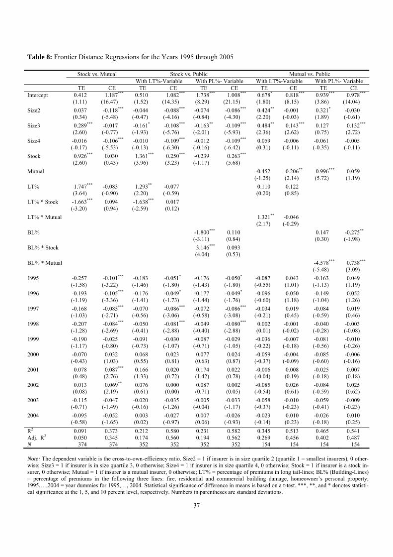
37

Table 8: Frontier Distance Regressions for the Years 1995 through 2005 Stock vs. Mutual Stock vs. Public Mutual vs. Public

With LT%-Variable With PL%- Variable With LT%-Variable With PL%- Variable TE CE TE CE TE CE TE CE TE CE

Intercept 0.412 1.187*** 0.510 1.082*** 1.738*** 1.008*** 0.678* 0.818 *** 0.939*** 0.978***

(1.11) (16.47) (1.52) (14.35) (8.29) (21.15) (1.80) (8.15) (3.86) (14.04)

Size2 0.037 -0.118*** -0.044 -0.088*** -0.074 -0.086*** 0.424** -0.001 0.321* -0.030

(0.34) (-5.48) (-0.47) (-4.16) (-0.84) (-4.30) (2.20) (-0.03) (1.89) (-0.61)

Size3 0.289 *** -0.017 -0.161 * -0.108*** -0.163** -0.109*** 0.484** 0.143 *** 0.127 0.132***

(2.60) (-0.77) (-1.93) (-5.76) (-2.01) (-5.93) (2.36) (2.62) (0.75) (2.72)

Size4 -0.016 -0.106*** -0.010 -0.109*** -0.012 -0.109*** 0.059 -0.006 -0.061 -0.005

(-0.17) (-5.53) (-0.13) (-6.30) (-0.16) (-6.42) (0.31) (-0.11) (-0.35) (-0.11)

Stock 0.926 *** 0.030 1.361 *** 0.250*** -0.239 0.263***

(2.60) (0.43) (3.96) (3.23) (-1.17) (5.68)

Mutual -0.452 0.206 ** 0.996*** 0.059

(-1.25) (2.14) (5.72) (1.19)

LT% 1.747 *** -0.083 1.293 ** -0.077 0.110 0.122

(3.64) (-0.90) (2.20) (-0.59) (0.20) (0.85)

LT% * Stock -1.663 *** 0.094 -1.638 *** 0.017

(-3.20) (0.94) (-2.59) (0.12)

LT% * Mutual 1.321** -0.046

(2.17) (-0.29)

BL% -1.800*** 0.110 0.147 -0.275**

(-3.11) (0.84) (0.30) (-1.98)

BL% * Stock 3.146*** 0.093

(4.04) (0.53)

BL% * Mutual -4.578*** 0.738***

(-5.48) (3.09)

1995 -0.257 -0.101*** -0.183 -0.051* -0.176 -0.050* -0.087 0.043 -0.163 0.049

(-1.58) (-3.22) (-1.46) (-1.80) (-1.43) (-1.80) (-0.55) (1.01) (-1.13) (1.19)

1996 -0.193 -0.105*** -0.176 -0.049* -0.177 -0.049* -0.096 0.050 -0.149 0.052

(-1.19) (-3.36) (-1.41) (-1.73) (-1.44) (-1.76) (-0.60) (1.18) (-1.04) (1.26)

1997 -0.168 -0.085*** -0.070 -0.086*** -0.072 -0.086*** -0.034 0.019 -0.084 0.019

(-1.03) (-2.71) (-0.56) (-3.06) (-0.58) (-3.08) (-0.21) (0.45) (-0.59) (0.46)

1998 -0.207 -0.084*** -0.050 -0.081*** -0.049 -0.080*** 0.002 -0.001 -0.040 -0.003

(-1.28) (-2.69) (-0.41) (-2.88) (-0.40) (-2.88) (0.01) (-0.02) (-0.28) (-0.08)

1999 -0.190 -0.025 -0.091 -0.030 -0.087 -0.029 -0.036 -0.007 -0.081 -0.010

(-1.17) (-0.80) (-0.73) (-1.07) (-0.71) (-1.05) (-0.22) (-0.18) (-0.56) (-0.26)

2000 -0.070 0.032 0.068 0.023 0.077 0.024 -0.059 -0.004 -0.085 -0.006

(-0.43) (1.03) (0.55) (0.81) (0.63) (0.87) (-0.37) (-0.09) (-0.60) (-0.16)

2001 0.078 0.087*** 0.166 0.020 0.174 0.022 -0.006 0.008 -0.025 0.007

(0.48) (2.76) (1.33) (0.72) (1.42) (0.78) (-0.04) (0.19) (-0.18) (0.18)

2002 0.013 0.069** 0.076 0.000 0.087 0.002 -0.085 0.026 -0.084 0.025

(0.08) (2.19) (0.61) (0.00) (0.71) (0.05) (-0.54) (0.61) (-0.59) (0.62)

2003 -0.115 -0.047 -0.020 -0.035 -0.005 -0.033 -0.058 -0.010 -0.059 -0.009

(-0.71) (-1.49) (-0.16) (-1.26) (-0.04) (-1.17) (-0.37) (-0.23) (-0.41) (-0.23)

2004 -0.095 -0.052 0.003 -0.027 0.007 -0.026 -0.023 0.010 -0.026 0.010

(-0.58) (-1.65) (0.02) (-0.97) (0.06) (-0.93) (-0.14) (0.23) (-0.18) (0.25)

R2 0.091 0.373 0.212 0.580 0.231 0.582 0.345 0.513 0.465 0.541Adj. R2 0.050 0.345 0.174 0.560 0.194 0.562 0.269 0.456 0.402 0.487N 374 374 352 352 352 352 154 154 154 154 Note: The dependent variable is the cross-to-own-efficiency ratio. Size2 = 1 if insurer is in size quartile 2 (quartile 1 = smallest insurers), 0 other-wise; Size3 = 1 if insurer is in size quartile 3, 0 otherwise; Size4 = 1 if insurer is in size quartile 4, 0 otherwise; Stock = 1 if insurer is a stock in-surer, 0 otherwise; Mutual = 1 if insurer is a mutual insurer, 0 otherwise; LT% = percentage of premiums in long tail-lines; BL% (Building-Lines) = percentage of premiums in the following three lines: fire, residential and commercial building damage, homeowner’s personal property; 1995,…,2004 = year dummies for 1995,…, 2004. Statistical significance of difference in means is based on a t-test. ***, **, and * denotes statisti-cal significance at the 1, 5, and 10 percent level, respectively. Numbers in parentheses are standard deviations.