The Effect of Transfer Programs on Labor Supply in the

Presence of Preference Heterogeneity and Variable Takeup

Robert MoffittJohns Hopkins University

April, 2004

An early version of this paper was presented at the SITE Conference, Stanford, August 1, 2003. The author would like to thank the National Institute of Child Health and Human Developmentfor research support and Jiawei Chen and Berna Demiralp for research assistance.

welfls1_v2.wpd4/25/04

Abstract

Recent developments in the analysis of treatment effects have emphasized models in

which those effects are heterogeneous in the population. The implication of these models is

there is no single effect of a treatment but rather that the effect depends upon where in the

population distribution of observables and unobservables the treatment effect is measured. This

paper revisits the estimation of the effects of transfer programs on labor supply within this new

framework. Both preference heterogeneity and variable takeup must be accounted for in this

problem. The paper proposes a semiparametric approach and applies it to a 1991 cross-section

of the Survey of Income and Program Participation.

The recent burgeoning literature on the identification and estimation of treatment effect

models has clarified a number of issues. One of the most important is that treatment effects can

be heterogeneous, meaning that the effect of a treatment on a unit being treated depends on both

unobservable and observable characteristics of that unit (Imbens and Angrist (1994), Heckman

and Vytlacil (1999, 2000, 2001); see also Heckman and Robb (1985) and Björklund and Moffitt

(1987) for earlier studies of heterogeneous response to treatments). This implies that the

average effect of a treatment on a population or subpopulation will depend upon the distribution

of those characteristics and where in that distribution the treatment effect occurs, and hence that

seeking to estimate “the” effect of a treatment on an outcome is ill-defined because there is no

single effect.

Nevertheless, this point has had little effect on practice, for most causal effect studies

continue to estimate only a single effect of a program (for two exceptions see Aakvik et al., 2002

and Carneiro et al., 2003, both of whom attempt to estimate a broader range of effects). This

paper reports the estimation of such heterogeneous treatment effects for the case of the effect of

welfare programs on labor supply. There is a large literature on this subject (for reviews, see

Blundell and MaCurdy, 1999; Moffitt, 1992, 2002) extending back to the 1960s and1970s,

including studies of the effect of the negative income tax. However, this literature, for the most

part, assumed homogeneous effects of treatment on labor supply (an exception is the nonlinear

budget constraint literature, which partially, but not fully, relaxed the homogeneity assumption,

as discussed below).

In addition to preference heterogeneity, variable takeup is a key feature of the study of

2

transfer programs and their effects on work effort. Participation rates in welfare programs

changes over time and varies across areas and demographic groups. If there is self-selection

into the program on the basis of preferences for work, the average effect of welfare on labor

supply will change as participation rates on welfare move around. This could explain some of

the wide dispersion in estimated effects of welfare in the past literature, for there is substantial

variation in welfare participation rates in the U.S. both in cross-section and time-series and the

samples used in past studies have been taken from different points in time and from different

groups.

The approach to estimating the heterogeneous treatment effect model taken in this paper

is relatively simple and is intended to be practicable to estimate in applied work. The model is

formulated as a two-equation reduced form model which is nonlinear in the parameters and

which can be estimated by simple nonlinear least squares. The unknown functions in the model

are set within a conventional regression context and are approximated with series methods. Both

observables and unobservables are treating semiparametrically to obtain maximal flexibility in

the specification.

Section I lays out a particular semiparametric formulation of the basic treatment effect

model with heterogeneous effects and proposes a simple estimation method for it. Section II

applies it to the static labor supply model in the presence of welfare programs. The empirical

analysis is reported in Section III.

3

I. A Formulation of the Heterogeneous Treatment Effects Model

Let yi be an outcome variable for individual i, Di a dummy variable indicating

participation in the program, and Zi an instrumental variable with a multinomial distribution.

Ignoring observables other than these for the moment, an unrestricted model can be written

yi = $i + "iDi (1)

* Di = k(Zi, *i) (2)

* Di = 1(Di $ 0) (3)

where $i and "i are scalar random parameters and *i is a vector of random parameters. All

parameters are allowed to be individual-specific. Eqn(1) is to be interpreted as a description of

potential outcomes, not just a description of how yi varies with Di in any particular population;

that is, "i is to be interpreted as the effect on yi resulting from a switch from Di=0 to Di=1 i.e.,as

the causal effect of Di on yi for individual i. Hence "i is the object of interest. What can be

estimated, however, is only the mean "i on some set of populations. The estimable object of

interest is E("i | Di), where

E(yi | Di) = E($i | Di) + E("i | Di) Di (4)

To see which of this class of objects can be identified as well as estimated, we work with

the reduced form:

1 Given the generality of (2), a monotonicity assumption is also needed to insure that Mk/MZ is of the same sign for all i. See Imbens and Angrist (1994).

4

E(yi | Zi=z) = E($i | Zi=z) + E("i | Di=1, Zi=z) Prob(Di=1 | Zi=z) (5)

E(Di | Zi=z) = Prob [k(z, *i) $ 0] (6)

We make the following assumptions:

A1. E( $i | Zi=z) = $

A2. E("i | Di=1, Zi=z) = g[E(Di=1 | Zi=z)]

Assumptions A1 and A2 are mean independence assumptions needed for Zi to be a valid

instrument. They state that the mean of the random intercept and conditional mean of the

random coefficient, respectively, are, in the former case, independent of Zi and, in the latter case,

dependent only on the fraction treated and not directly on Zi.1

With these assumptions, and letting F(Zi)=E(Di=1 | Zi), (5) and (6) imply that

yi = $ + g[F(Zi)] F(Zi) + ,i (7)

Di = F(Zi) + <i (8)

where F is a proper probability function and where E(,i | gF ) = E(<i | F ) = 0 by construction.

Nonparametric identification of the parameters of (7) and (8) is straightforward given that

2 In the special case that the support of Zi in the data contains an element s.t. F(Zi)=0, nonormalization is necessary.

3 In the application below, cross-equation weights will be used as well. Two-stageestimation (i.e., two-stage least squares) is an option and corresponds to instrumental variablesestimation when k is allowed to be fully nonparametric in Zi. However, if k is considered

5

Di is binary and Zi has a multinomial distribution. F(Zi) is identified at each point Zi=z from

the population mean of Di at that z. The parameter $ and the function g[F(Zi)] at Zi=z are

identified provided a normalization is made to the g function, e.g., g[F(Z1)]=1.2 The treatment

effects discussed in the literature are all defined by g: the average treatment effect is g(1); the

effect of the treatment on the treated a fraction Fj is treated is g(Fj); the local average treatment

effect between two participation fractions Fj and Fj’ is [Fjg(Fj)-Fj’g(Fj’)]/(Fj-Fj’); and the

marginal treatment effect at some point Fj is My/MF=g’(Fj)Fj+g(Fj), which must be obtained by

some smoothing method given the multinomial assumption on Zi.

We will approach the problem nonparametrically. We will be nonparametric on g and k

(but parametric on F), approximating each with a series expansion using regression splines with

parameter vectors 21,and 22, respectively (Newey, 1997). The series expansion approach is

nonparametric in the limit but can also be treated as a flexible-form parametric approach. In

addition, it is computationally convenient for a fixed order of the series because splines lead to

easily estimable nonlinear functions. Consequently, (7) and (8) can be estimated by joint

nonlinear least squares (NLS) with any simple regression package. The estimation problem is

Min 3 w1i [yi - $ - g[F(k(Zi,22)); 21] F(k(Zi,22)) ]2 + 3 w2i [Di - F(k(Zi,22))]2 21,22 i i (9)

where w1i and w2i are possible weights to improve efficiency.3

instead to be a smoothed function of Zi or if Zi is continuous, a first-stage predicted F shouldnot be inserted into a nonlinear function g.

6

Adding a vector of exogenous observables Xi to the model will also be approached

nonparametrically, again building off of the conventional linear regression model. The model is

now

yi = "iDi + hi(Xi) + ji(Xi)Di (10)

* Di = k(Zi, Xi, *i) (11)

* Di = 1(Di $ 0) (12)

where it is understood that a normalization of ji(Xi) is necessary to separately identify "i.

We assume

B1. E[ hi(Xi) | Xi=x, Zi=z) = h(x) (13)

B2. E("i | Di=1, Xi=x, Zi=z) = g[E(Di=1 | Xi=x, Zi=z), x] (14)

B3. E(ji(Xi) | Di=1, Xi=x, Zi=z) = j[E(Di=1 | Xi=x, Zi=z), x] (15)

Then (10)-(12) can be rewritten

yi = g[F(Zi,Xi), Xi] F(Zi,Xi) + h(Xi) + j [F(Zi,Xi), ,Xi] F(Zi,Xi) + ,i (16)

Di = F(Zi,Xi) + <i (17)

where, again, the errors are mean-independent of the regressors by construction. In current

7

work,

we employ parametric, linear forms for X but in future work we will incorporate more flexible

forms again using regression splines..

II. Labor Supply and Welfare Programs

Utility in the presence of welfare programs can be written as

U(H,Y; 2) - NP (18)

where H=hours of work, Y=disposable income, P is a dichotomous indicator equal to 1 if the

individual is on welfare and 0 if not, and 2 is a vector of taste parameters which vary across

individuals (individual subscripts omitted). The parameter N can be interpreted as representing

welfare stigma (Moffitt, 1983) or as the utility value of the fixed costs associated with being on

welfare (money and time costs of application, complying with reporting and other requirements,

etc). The separability of U and P in (18) will be relaxed in the empirical work but is maintained

in this section to clarify the importance of the cost term.

The individual is assumed to face a parametric hourly wage rate W and to have available

exogenous, non-transfer nonlabor income N. The welfare benefit formula is B = G - tWH - rN

and hence the budget constraint is

Y = W(1-t)H + G + (1-r)N if P = 1 (19)

8

Y = WH + N if P = 0 (20)

~ ~ ~ Letting H(W,N; 2) be the labor supply function along a linear budget constraint with net wage W ~and virtual nonlabor income N resulting from the maximization of U(H,Y;2), the labor supply

function can be written

H = H [ W(1 - tP) , N + P(G - rN) ; 2] (21)

The determination of P is described by

P* = V [ W(1-t), G + N(1-t) ; 2 ] - V [W,N ; 2] - N (22)

P = 1(P*$0) (23)

where V is the indirect utility function. Equation (21) is a conditional-on-P function analogous

to eqn (1) and eqn(22)-(23) is a P function analogous to eqn(2)-(3). Note that the presence of

fixed costs suggests a theoretical basis for exclusion restrictions if there are observed

determinants of such costs which are exogenous to labor supply.

Heterogeneity in 2 induces heterogeneity of the response of H to P for two separate

reasons. First, such heterogeneity results in variation across the population in the response to net

wages and nonlabor income in general, and would arise even if P were exogenous to labor supply

unobservables. This is a conventional form of heterogeneity and, in linear-in-parameters models,

merely implies that population means of the parameters are estimated. Second, and more

important, such heterogeneity implies that a shift in either budget constraint parameters or fixed

4 The same situation arises in the analysis of the labor supply effects of positive taxsystems, where 100 percent participation is generally assumed.

9

costs will change the distribution of 2 in the participant population, and this will induce a change

in the effect of P on H as well. An exception occurs when only a separable intercept is random,

as in the model (individual subscripts added)

~ ~ Hi = 20i + h(Wi,Ni; 21) (24)

In this case, expansions and contractions of the participant population induce compositional shifts

in the difference in mean labor supply of participants and nonparticipants, creating bias in simple

comparisons (Moffitt, 1983), but there is no difference across the population in the response to

participation once it occurs. This stands in contrast to the models of Burtless and Hausman

(1978) and Hausman (1981), where heterogeneity was located in a random income effect. Both

approaches are restrictive relative to a model in which all parameters are allowed to be

heterogeneous.

The presence of N is important to interpretation and identification in the model. If there

are no fixed costs then 100 percent of eligibles participate, and in this case there is no variation in

P conditional on W, N, t, G, and 2.4 It is more difficult to separate the effects of heterogeneity in

2 in the conditional labor supply functions from the heterogeneous effects of participation per se

because variations in participation can only be induced by changes in W, N, t, and G. Effectively,

P does not belong in the equation for H at all in that case. If the conditional-on-P demand

function can be identified and estimated, the participation function can be derived from it.

10

The sign of the effect of changes in participation on labor supply responses is ambiguous.

As the program becomes more generous, for example, or as fixed costs fall, those with lesser

utility gains from entering welfare than those already on welfare will enter the program.

However, there is no necessary relationship between the value of utility gains and an individual’s

value of 2, for the wage and income elasticities contained in 2 merely indicate how much of the

response to an increase in program generosity is taken in the form of leisure rather than

consumption. There is no a priori reason to expect those with lesser utility gains to welfare to be

have a greater or lesser desire for leisure relative to consumption compared to those with greater

utility gains. Thus the way in which the mean labor supply effects of welfare change with

participation must be resolved empirically.

In our initial empirical work we shall simply estimate g as a function of P using flexible

forms for the participation function without any structure from the underlying utility model

imposed. Imposing a utility structure is reserved for future work.

III. Data

The empirical exercises reported here use a 1991 cross section taken from the Survey of

Income and Program Participation (SIPP). The year 1991 is the last year that can be confidently

regarded as being prior to the major reforms in the Aid to Families with Dependent Children

(AFDC) program, reforms which began in various states in 1992 and culminated in federal

legislation in 1996. Those reforms altered the program in ways that make the simple model of

the program described above inappropriate because work requirements, time limits, and other

11

important features were introduced. The SIPP is a representative household survey of the U.S.

noninstitutional population consisting of a series of relatively short (9-to-32 month) panels begun

in 1984. Families are interviewed every four months and are asked a complete set of labor

force, income, and transfer program questions for each of the four months prior to the interview

date. Each panel consists of a set of rotation groups whose members are interviewed on a rolling

set of four-month cycles, so that families are being interviewed every month. Some panels are

begun before others are finished, and therefore there are often more than one panel in the field at

a given time We are interested in months close to April because they are close to tax filing dates

and hence should aid in the recall of economic information (the same reason the March Current

Population Survey is conducted in that month); we take all families interviewed in either March,

April, May, or June of 1991. The panels begun in February 1990 and February 1991 covered this

period, so the sample is drawn from both panels and pooled. We draw information only for the

month prior to interview because that is least likely to be affected by recall bias. We select all

women 14-55 who were unmarried and had children under 18 in the family as of the month prior

to interview and, to concentrate on the welfare-eligible population, we take only those with

education less than or equal to 12. We use the data on average hours worked per week, nonlabor

income, and demographic characteristics as of the prior month. Welfare participation is measured

as having been on the AFDC in that month. We match government data on AFDC guarantee

levels onto the data set, using state of residence as the matching variable. There are 4,749

observations in the sample. The means of the variables are shown in Table 1.

The chief advantage of the SIPP over alternative full-population U.S. data sets such as the

Current Population Survey (CPS), the Michigan Panel Study on Income Dynamics (PSID), or

5 Many of these data sets now ask respondents to report program participation separatelyfor each of the 12 months in the prior calendar year, and sometimes labor supply for those sameperiods, but it is very difficult to line up demographics and earnings with those months.

6 There were minor exceptions to this rule resulting from small set-aside amounts, anallowance of a lower tax rate for the first four months of work, and others, but these did not alterlabor supply except in narrow ranges.

12

related data sets, is that transfer income information is available in the month prior to interview

and can be matched for that month to labor supply and demographic information. The CPS,

PSID, and many other data sets only have information on whether any transfer program

participation occurred in the previous (January-December) calendar year obtained from questions

asked of respondents in the following Spring. Aside from recall error in such questions, it is not

possible to line up demographic characteristics and labor supply variables for the actual periods in

which the individual was on welfare with such data. As a consequence, most studies published in

the 1980s and before related average hours of work in the prior year to whether any program

participation took place in that, which is clearly a misspecified model.5 This does mean,

however, that the mean participation rate in our sample (17 percent) is considerably lower than

that in most prior studies (approximately one-third or more) because the prior studies only used

cumulative annual experience to define their variables. Our data should result in more accurate

estimates given the use of labor supply and program participation data measured at the same time.

Identification of the model is achieved by using a particular feature of the AFDC program,

namely, that the tax rate on earnings between 1981 and 1991 was 100 percent.6 As a

consequence, essentially no women on AFDC worked. Our data is consistent with this feature,

for less than 10 percent of women reporting AFDC participation in the past month also reported

positive hours of work. With this feature, hours of work on welfare are approximately zero and

13

hence there is effectively no variation in them. The estimation of the labor supply effects of

AFDC reduces in this case to an estimate of the difference in the hours that a woman would work

off welfare and zero. Because neither t nor G affects the former hours of work, both of these

variables satisfy the exclusion condition that they affect the probability of program participation

but do not directly affect labor supply. Because t does not vary, G is used as the instrument.

IV. Results

The model specification used in the exercise is the following:

yi = Xi$ + [Xi8 + g(F(Xi* + 0Gi))] F(Xi* + 0Gi) + ,i (25)

Di = F(Xi* + 0Gi) + <i (26)

where Gi is the AFDC guarantee, g is a spline function, and F is the normal c.d.f. Denote ui as a

2x1 column vector of residuals for individual i, the first being the residual in (25) and the second

being the residual in (26). Then the unknown parameters in both equations, which we denote 2,

are estimated by the criterion

n ^ 2 = Arg Min 3 ui' S-1 ui (27)

2 i=1

^where S is a 2x2 matrix of variances of the residuals obtained from an unweighted first-stage

estimation. The covariance matrix of the estimated 2 is calculated as

^ n ^ -1 -1 n ^ -1 ^ -1 n ^ -1 -1 Var (2) = ( 3 Mi' S Mi) ( 3 Mi' S uiui' S Mi) ( 3 Mi' S Mi) (28) i=1 i=1 i=1

14

where Mi is the 2xK matrix of derivatives of the functions in each equation w.r.t. the K

parameters in the model.

Estimates of several specifications of the model are shown in Table 2. The first column

is a constant-effect model with neither observed nor unobserved heterogeneity in the effect of

welfare program participation on labor supply. The negative effect of participation is estimated

at about -14 hours per week. Most of the coefficients on observed variables affecting the level of

labor supply are significant in the expected direction, as are most of those affect participation

probabilities. The guarantee has a significant positive effect on participation as well.

An issue in these models is the support of the predicted probabilities, which will

determine the range over which heterogeneous effects can be estimated. Figure 1 shows a

histogram of the residual of a regression of the guarantee on the other variables in the

participation equation, showing it has considerable range. This is not surprising because it is a

state-specific variable and it is known that welfare benefits vary greatly across states in the U.S.

Figure 2 shows a histogram of the predicted probabilities from the participation regression,

showing that many are very close to zero but there is a significant tail to the right. This suggests

that the data will be able to provide estimates of the effect of the treatment on the treated but not

of the ATE. However, this distribution is generated in part by the dispersion in the X vector, and

the position taken here is that that variation is useful only if the partially linear model is correct.

In its absence, only the variation in the guarantee conditional on X provides participation

variation used in the estimation of labor supply effects of participation. Figure 3 shows a

histogram of the participation rate differences, equal to the difference in the participation rate for

an individual with and without the welfare guarantee. Clearly the support of this distribution is

7 The sum of the splines is also generally insignificant.

15

much less than that of the overall participation distribution.

That the guarantee has a positive effect is illustrated in Figure 4, which shows a kernel

regression of welfare participation on the guarantee residual described above. The relationship is

clearly positive.

Returning to Table 2, column (2) shows the effect of adding a linear-in-F term to the

return. Its coefficient is significantly negative, implying that the negative effect of welfare grows

with participation, suggesting that those brought in on the margin have greater labor supply

reductions than those initially drawn into the program. However, this effect is weakened in

significance in column (3) when observed heterogeneity is added, although its effect is greater in

magnitude. The negative effects of welfare on labor supply are significantly correlated with

many observations, and are more negative for those with more education, fewer young children,

and larger families; for those who are older; and for white women. The participation equation

demonstrates that these variables are correlated with participation, and is clear that they explain

part of the implied unobserved heterogeneity in effects estimated in the prior model.

The last three columns add splines at the 25th, 50th, and 75th percentile points of the

predicted participation distribution, with little success. The splines at the median is never

significant, and that at the 25th percentile point blows up the model. Only the effect at the 75th

percentile is significant, and indicates that the negative effects on labor supply are smaller for

those with participation probabilities higher than that point. Thus, once again, there is little

evidence of unobserved heterogeneity in labor supply responses.7

Figures 5 and 6 demonstrate this point graphically. Figure 5 shows a histogram of the

16

distribution of the g function obtained by setting the coefficients on the participation rates in that

function equal to zero, and shows the distribution of effects from observables alone. A rather

large spread of effects is shown. Figure 6 shows the same histogram after the effects of the

participation rate are added in (column (6) of Table 2 is used). The spread widens slightly, but

only very little.

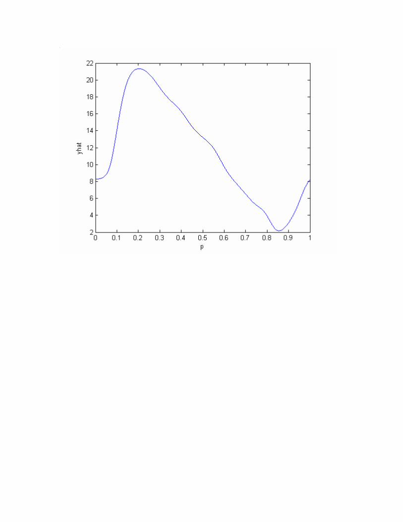
Figures 7 and 8 show kernel regressions of hours on predicted participation, and of the

slope of the y function w.r.t. predicted partication, also regressed on predicted participation. The

latter corresponds to the marginal treatment effect in the model. Clearly, there remains, on

average, some unobserved heterogeneity in response in the population even after conditioning on

the X vector, with more negative responses for those drawn into the program. However, the

standard errors are sufficiently high as to make these estimates highly uncertain.

V. Conclusions

This paper has reported an exercise in estimating whether the effect of participation in the

U.S. AFDC program on labor supply of single mothers varies across individuals. The exercise

uses a relatively simple nonlinear least squares approach to the problem combined with regression

splines to approximate the heterogeneity of unobserved labor supply effects. The results show

that there is indeed great heterogeneity in those effects but that are dominated by effects which

vary with observables. The variance in unobserved heterogeneity after observed heterogeneity is

controlled for is small by comparison.

17

VI. References

Aakvik, Arild; James J. Heckman; and Edward J. Vytlacil. 2002. “Estimating Treatment Effectsfor Discrete Outcomes When Responses to Treatment Vary: An Application to NorwegianVocational Rehabilitation Programs.” Mimeo.

Björklund, A. and R. Moffitt. 1987. “The Estimation of Wage and Welfare Gains in Self-Selection Models." Review of Economics and Statistics 69: 42-49.

Blundell, R. and T. MaCurdy. 1999. "Labor Supply: A Review of Alternative Approaches" ” InHandbook of Labor Economics, Vol. 3A, eds. O. Ashenfelter and D. Card. Amsterdam and NewYork: Elsevier.

Burtless, G. and J. Hausman. 1978. "The Effect of Taxaton on Labor Supply: The Gary IncomeMaintenance Experiment." Journal of Political Economy 86: 1103-1130.

Carneiro, Pedro; James J. Heckman; and Edward Vytlacil. 2003. “Understanding WhatInstrumental Variables Estimate: Estimating Marginal and Average Returns to Education.” Mimeo.

Hausman, J. "Labor Supply." 1981. In How Taxes Affect Economic Behavior, eds. H. Aaron andJ. Pechman. Washington: Brookings Institution.

Heckman, J. and R. Robb. 1985. "Alternative Methods for Evaluating the Impact ofInterventions." In Longitudinal Analysis of Labor Market Data, eds J. Heckman and B. Singer.Cambridge University Press..

Heckman, J. and E. Vytlacil. 1999. "Local Instrumental Variables and Latent Variable Modelsfor Identifying and Bounding Treatment Effects." Proceedings of the National Academy ofSciences 96 (April): 4730-4734.

Heckman, J. and E. Vytlacil. 2000. “Causal Parameters, Structural Equations, Treatment Effectsand Randomized Evaluations of Social Programs.” Mimeo. UC and Stanford.

Heckman, J. and E. Vytlacil. 2001. “Policy-Relevant Treatment Effects.” American EconomicReview 91 (May): 107-111.

Imbens, G. and J. Angrist. 1994. "Identification and Estimation of Local Average TreatmentEffects." Econometrica 62: 467-76.

Moffitt, R. 1983. "An Economic Model of Welfare Stigma." American Economic Review 73(December: 1023-1035.

18

Moffitt, R. 1992. “Incentive Effects of the U.S. Welfare System: A Review.” Journal ofEconomic Literature 30 (March): 1-61.

Moffitt, R. 2002. “Welfare Programs and Labor Supply.” In Handbook of Public Economics,Vol.4, eds. A. Auerbach and M. Friedman. Chicago: University of Chicago Press.

Newey, W. 1997. “Convergence Rates and Asymptotic Normality for Series Estimators.” Journalof Econometrics 79(1997): 147-168.

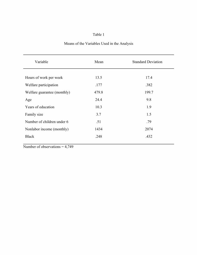
Table 1

Means of the Variables Used in the Analysis

Variable Mean Standard Deviation

Hours of work per week 13.5 17.4

Welfare participation .177 .382

Welfare guarantee (monthly) 479.8 199.7

Age 24.4 9.8

Years of education 10.3 1.9

Family size 3.7 1.5

Number of children under 6 .51 .79

Nonlabor income (monthly) 1434 2074

Black .248 .432

Number of observations = 4,749

Table 2

Results of the Estimation

(1) (2) (3) (4) (5) (6)

g function

Constant -13.7*(2.35)

-2.5(4.0)

71.5*(16.2)

64.5(41.0)

-8632(6902)

81.3*(35.1)

F -- -22.6*(5.5)

-44.5(36.1)

52.8(263.1)

4 84.0(269.7)

Max(0,F-.25F) -- -- -- -- -4 --

Max(0,F-.50F) -- -- -- -102.0(250.1)

-119.2(267.5)

-228.3(268.6)

Max(0,F-.75F) -- -- -- -- -- 83.3*(35.0)

lambda

Education -- -- -8.3*(.88)

-8.1*(1.3)

-6.6*(.97)

-5.5*(.73)

Age -- -- -1.0*(.50)

-.90*(.50)

.12(.35)

-.48*(.17)

Black -- -- 13.8*(.23)

13.4*(3.9)

13.4*(.18)

9.5*(2.86)

Children < 6 -- -- 8.4*(5.0)

9.1*(4.8)

17.1*(3.9)

10.3*(3.0)

Family size -- -- -2.3*(1.20)

-2.8*(1.2)

-3.8*(1.2)

-5.0*(1.0)

Nonlabor Y -- -- -.07(.34)

-.11(.37)

-.02*(.01)

-1.03(.76)

Table 2 (continued)

Results of the Estimation

(1) (2) (3) (4) (5) (6)

beta

Constant -19.1*(-1.7)

-19.7*(1.6)

-42.6*(2.6)

-41.9*(3.0)

-34.1*(2.4)

-36.8*(2.3)

Education 1.96*(.14)

1.88*(.14)

2.73*(.32)

2.84*(.31)

2.67*(.26)

2.86*(.25)

Age .74*(.03)

.73*(.03)

1.57*(.14)

1.45*(.13)

1.01*(.10)

.92*(.08)

Black -2.01*(.51)

-1.70*(.50)

-2.43*(.88)

-2.58*(.85)

-2.62*(.70)

-2.58*(.69)

Children < 6 .91*(.48)

1.73*(.50)

3.11*(1.20)

2.55*(1.13)

.73(.78)

.67(2.86)

Family size -.73*(.16)

-.62*(.16)

-.14(.23)

-.13(.22)

-.03(.21)

.17(3.02)

Nonlabor Y -.03*(.01)

-.01(.01)

-.04*(.02)

-.03*(.02)

-.03(.02)

.00(1.00)

delta

Constant -.88*(.20)

-1.32*(.21)

-1.12*(.15)

-1.09*(.15)

-1.21*(.18)

-1.13*(.17)

Education -.07*(.03)

-.05*(.01)

-.10*(.01)

-.10*(.01)

-.08*(.02)

-.08*(.01)

Age .02*(.00)

.02*(.00)

.04*(.00)

.04*(.00)

.03*(.00)

.03*(.00)

Black .44*(.06)

.42*(.06)

.25*(.05)

.27*(.05)

.30*(.06)

.35*(.06)

Table 2 (continued)

Results of the Estimation

(1) (2) (3) (4) (5) (6)

Children < 6 .49*(.04)

.49*(.04)

.39*(.03)

.41*(.03)

.46*(.03)

.51*(.03)

Family size -.05*(.02)

-.03(.02)

-.01(.02)

-.02(.02)

-.03(.02)

-.05*(.02)

Nonlabor Y -.14*(.02)

-.13*(.02)

-.01*(.00)

-.02*(.00)

-.06*(.01)

-.07*(.01)

nu

Guarantee .07*(.01)

.08*.01)

.04*(.01)

.04*(.01)

.04*(.01)

.06*(.01)

Notes:Standard errors in parentheses*: significant at the 10 percent level

Nonlabor income and guarantee variables divided by 100

0 0.1 0.2 0.3 0.4 0.5 0.6 0.7 0.8 0.9 10

200

400

600

800

1000

1200

1400

1600

1800

2000histogram of phat

0 0.1 0.2 0.3 0.4 0.5 0.6 0.7 0.8 0.9 10

500

1000

1500

2000

2500

3000histogram of phat3-phat2

-150 -100 -50 0 50 1000

100

200

300

400

500

600

700

800

900histogram of the estimate of alpha(p) at p=0

-140 -120 -100 -80 -60 -40 -20 0 20 40 600

100

200

300

400

500

600

700

800

900histogram of the estimate of alpha(p)