THE EFFECT OF UNCERTAINTY ON INVESTMENT: EVIDENCE FROM TEXAS OIL DRILLING

Ryan Kellogg*

January, 2012

Abstract

Despite widespread application of real options theory in the literature, the extent to which firms actually delay irreversible investments following an increase in the uncertainty of their environment is not empirically well-known. This paper estimates firms’ responsiveness to changes in uncertainty using detailed data on oil well drilling in Texas and expectations of future oil price volatility derived from the NYMEX futures options market. Using a dynamic model of firms’ investment problem, I find that oil companies respond to changes in expected price volatility by adjusting their drilling activity by a magnitude consistent with the optimal response prescribed by theory.

___________________________ *Department of Economics, University of Michigan, and NBER. kelloggr@umich.edu. I am grateful for financial support from the OpenLink Fund at the Coleman Fung Risk Management Center. I thank Maximilian Auffhammer, Ruediger Bachmann, Robert Barsky, Nicholas Bloom, Severin Borenstein, Lutz Kilian, Kai-Uwe Kühn, Jeffrey Perloff, Robert Pindyck, Matthew Shapiro, and Catherine Wolfram for helpful comments, and I am also grateful for suggestions from numerous seminar and conference participants. I thank Reid Dorsey-Palmateer, Tay Feder, and Haili Pang for excellent research assistance.

1

1. Introduction

How do firms make decisions regarding irreversible investments in uncertain economic

environments? Such situations are common in a variety of industries: American Electric Power

must commence construction of new plants before knowing the future demand for electricity,

Boeing must sink costs into new airplane designs before orders from customers are realized, and

ExxonMobil must drill wells in the midst of a fluctuating price of oil. Each of these investments

is at least partially irreversible because the assets created cannot be fully appropriated to an

alternative use. In other words, these investments, once complete, become sunk costs.

The real options literature, beginning with Marschak (1949) and Arrow (1968) and

developed in Bernanke (1983), Pindyck (1991), and Dixit and Pindyck (1994), explains how

firms should time such investments. Real options theory views an irreversible investment as an

option in that, at any point in time, a firm may choose to either invest immediately or delay and

observe the evolution of the investment’s payoff. A key insight is that the option to delay has

value when future states of the world with positive returns to investing and states with negative

returns are both possible, even holding the expected future return constant at its current level.

Thus, in the presence of irreversibility and uncertainty, a naïve investment timing rule—proceed

with an investment if its expected benefit even slightly exceeds its cost—is suboptimal because it

does not account for the value of continuing to hold the option. Instead, firms should delay

irreversible investments until a significant gap develops between the investments’ expected

benefits and costs. Moreover, as uncertainty increases, real options theory tells us that the

incentive to delay should grow stronger and the gap between the expected benefit and cost

necessary to trigger investment should widen.

While real options theory therefore prescribes how firms should carry out irreversible

investments in uncertain environments, it is not empirically well-known how firms actually

proceed in such situations. In particular, the theory’s central prediction that firms should be more

likely to delay investment if uncertainty increases, all else equal, has received only limited

empirical scrutiny. The primary aim of this paper is therefore to assess the extent to which firms’

responses to changes in uncertainty align with the theory, using data on oil drilling activity in

Texas coupled with market expectations of the volatility of the future price of oil.

The need for empirical work in the real options literature is underscored by the existence

of numerous applications that assume firms optimally make decisions in the presence of

uncertainty. In industrial organization, Pakes (1986), Dixit (1989), Grenadier (2002),

Aguerrevere (2003), and Collard-Wexler (2010) model the implications of uncertainty and sunk

2

costs for investment, entry, and research and development in several settings and under various

forms of competition. The general dynamic oligopoly model of Ericson and Pakes (1995) is built

on a framework in which firms treat many decisions as options. In macroeconomics, Bernanke

(1983), Hassler (1996), Bloom (2009), and Bloom et al. (2007, 2011) construct models that

emphasize the importance of changes in economy-wide uncertainty in determining the level of

aggregate investment. Finally, in the environmental and resource economics literature, Arrow

and Fisher (1974), among others, discuss the role of uncertainty in dictating when “green”

investments should be undertaken.

I empirically examine the extent to which investments in oil wells respond to changes in

uncertainty using a unique dataset of well-level drilling activity in Texas. I combine these

drilling data with information from the New York Mercantile Exchange (NYMEX) on the

expected future price of oil and the expected future price volatility. The expected volatility is

derived from the NYMEX futures options market, in which volatility is implicitly traded and

priced. Under a hypothesis that the market is an efficient aggregator of information, the implied

volatility from futures options will incorporate more information than an expected volatility

measure derived from price histories alone.

I conduct my analysis using an econometric model of firms’ optimal drilling investment

in the presence of time-varying uncertainty. The model is based on Rust’s (1987) nested fixed

point approach but allows the volatility of the process governing state transitions to vary over

time. The use of this model allows me to do more than carry out a simple “yes/no” test of

whether or not firms respond to changes in expected oil price volatility: I can also compare the

magnitude of firms’ responses in the data to the magnitude prescribed by the model.

I find that the response of investment to changes in implied volatility is broadly

consistent with optimal decision-making. In the reference case specification, in which the

model’s auxiliary parameters and assumptions most closely match the data and institutional

setting, I find that the magnitude of firms’ collective response to volatility shocks aligns closely

with theory. Alternative specifications and assumptions lead to estimates of different

magnitudes, though these estimates remain qualitatively similar to the optimal response so long

as volatility expectations are measured using implied volatility from futures options. When I

instead measure expectations using historical price volatility, the estimated response of

investment to changes in volatility is attenuated and imprecise, reflecting the relatively weak

forecasting power of this measure.

There exist previous studies that have empirically examined whether investments respond

to changes in uncertainty, though without linking the magnitudes of the estimated effects to

3

theory. Several of these studies, like this one, focus on natural resource industries. Hurn and

Wright (1994), Moel and Tufano (2002), and Dunne and Mu (2010) examine the impact of

resource price volatility on offshore oil field investments, gold mine openings and closings, and

refinery investments, respectively. None of these papers uses implied volatility to measure

expected price volatility—the uncertainty measure is the historic realized variance of commodity

prices—and they collectively find mixed evidence on whether increases in volatility reduce

investment. Paddock, Siegel, and Smith (1988) shows that option pricing techniques yield more

accurate predictions of oil lease valuations than do traditional net present value calculations,

though without investigating the impact of changes in uncertainty over time. Other micro-

empirical work includes Guiso and Parigi (1999), which finds evidence from a cross-sectional

survey that Italian firms whose managers subjectively report high levels of expected demand

uncertainty tend to have relatively low levels of investment. List and Haigh (2010) meanwhile

provides experimental evidence that investment timing decisions of agents (drawn from student

and professional trader subject pools) are generally responsive to changes in payoff uncertainty.

Another set of papers in the macroeconomics literature measures the response of

aggregate output and investment to changes in economy-wide uncertainty, as measured by the

volatility of stock market returns or interest rates (Hassler 2001, Alexopoulos and Cohen 2009,

Fernandez-Villaverde et al. 2009, and Bloom 2009). A related work is Leahy and Whited (1996),

which examines firm-level investment and stock return volatilities. These papers generally find

that increases in volatility are associated with decreases in output or investment. However,

factors that influence the expected level of investments’ payoffs are difficult to proxy for in this

literature, and Bachmann et al. (2010) argues that a negative correlation between first and second

moment shocks can lead to downward-biased estimates of the effects of an increase in

uncertainty. Leahy and Whited (1996) also notes that fluctuations in stock returns likely reflect

the volatility of factors beyond those impacting the future revenues associated with new,

marginal investment opportunities.

This paper’s focus on the Texas onshore drilling industry as its object of study, combined

with the econometric modeling of the firms’ investment timing problem, confers valuable

advantages relative to previous work. First, I possess data at the level of each individual

investment—the drilling of each well—and need not rely on aggregate data or accounting data.

Second, the NYMEX futures and futures options markets provide measures of the expected level

and volatility of each investment’s expected return that, in principle, incorporate all available

information at the time of the investment. Such measures are not available in most industry

settings, and here they allow for a separation of first and second moment shocks. Finally, I take

4

advantage of the fact that oil production is a highly competitive industry, with no one firm able

to influence the price of oil, and I focus on oil fields in which common pool issues are not a

concern. I am therefore able to treat each firm’s investment decision as a single-agent dynamic

investment problem. This approach, which would be questionable in most other industries,

allows me to measure the magnitude of firms’ response to uncertainty relative to the theoretical

optimum, going beyond a simple test of whether or not firms respond to volatility shocks at all.

In what follows, I first discuss relevant institutional details of the Texas onshore drilling

industry and the datasets I use. Section 3 follows with a descriptive analysis of the data. The

remainder of the paper focuses on the construction and estimation of a structural model of the

drilling investment problem with time-varying uncertainty: section 4 presents the model, section

5 discusses the estimation procedure, and section 6 follows with the estimation results. Section 7

provides concluding remarks.

2. Institutional Setting and Data

2.1 Drilling description, types of wells used in this study, and drilling data

Oil and gas reserves are found in geologic formations known as fields that lie beneath the

earth’s surface, and the mission of an oil production company is to extract these reserves for

processing and sale. To recover the reserves, the firm needs to drill wells into the field. Drilling

is an up-front investment in future production; if a drilled well is successful in finding reserves, it

will then produce oil for a period of several years, requiring relatively small operating expenses

for maintenance and pumping. The firm does not know in advance how much oil will be

produced (if any) from a newly drilled well, though it will form an expectation of this quantity

based on available information, such as seismic surveys and the production outcomes of

previously drilled wells. The price that the firm will receive for the produced oil is also not

known with certainty at the time of drilling. Conversations with industry participants have

indicated that some, though not all, firms use the NYMEX market to hedge at least some of their

price risk. This use of the NYMEX indicates that risk aversion over future oil prices is unlikely

to influence drilling decisions, since any firm that is risk averse can hedge the price risk away.

Drilling costs range from a few hundred thousand dollars for a relatively shallow well

that is a few thousand feet deep to millions of dollars for a very deep well (as much as 20,000

feet deep). Once drilled, these costs are almost completely sunk: the labor and drilling rig rental

costs expended during drilling cannot be recovered, nor can the expensive steel well casing and

5

cement that run down the length of the hole. Drilling can therefore be modeled as a fully

irreversible investment.

Wells can be one of three types: exploratory, development, or infill. Exploratory wells are

drilled into new prospective fields, and if successful they can not only be productive themselves

but also lead to additional drilling activity. Development wells are those that follow the

exploratory well: they increase the number of penetrations into a recently discovered field in

order to drain its reserves. Finally, infill wells are drilled late in a field’s life to enhance an oil

field’s production by “filling in” areas of the reservoir that have not been fully exploited by the

pre-existing well stock.

In this paper, I exclude exploratory and development wells and analyze only the subset of

data corresponding to infill wells. This exclusion facilitates this study in two important ways.

First, examining only infill wells constrains the set of available drilling options to those that exist

within a finite, known set of fields. Thus, I need not be concerned with the creation of new

options through new field discoveries or leasing activity. Second, the majority of production

from a typical infill well takes place within the first year or two of the well’s life: because infill

wells tap only small isolated pools of oil that have been left behind by older wells in a field, their

productive life is quite short. Thus, I may rely on liquid near-term futures to provide expected

prices and volatilities that are relevant for these wells rather than less liquid long-term futures.

I also distinguish wells drilled in fields operated by a single firm from wells drilled in

fields operated by multiple firms. The process by which production companies acquire leases—

rights to drill on particular plots of land—often leads to situations in which several firms have

the right to drill in and produce from a single field (see Wiggins and Libecap 1985). This

division of operating rights leads to a common pool problem to the extent that each firm’s

actions lead to informational and extraction externalities for its neighbors, suggesting that in such

situations a dynamic game is needed to model firms’ drilling problem. This paper avoids this

substantial complication by focusing exclusively on wells drilled in sole-operated fields, for

which a single-agent model is sufficient to model drilling behavior.1

1 Industry participants have suggested that the degree of strategic interaction amongst firms drilling infill wells in common pool fields may be limited in practice because infill drilling targets tend to be small pools that are geologically isolated from other parts of the field. In addition, the TRRC regulates the minimum distance from a neighbor’s lease at which a well may be drilled. Correspondingly, the time series of infill drilling in all fields, including common pools, is very similar to that for sole-operated fields (see appendix figure A1). I nevertheless focus my analysis on sole-operated fields to be conservative, though estimating the model using the full sample of infill wells yields very similar results to those presented here (the estimate of β is 1.117).

6

I obtained drilling data from the Texas Railroad Commission (TRRC), yielding

information regarding every well drilled in Texas from 1977 through 2003.2 These data identify

when each well was drilled, which field it was drilled in, whether it was drilled for oil or for gas,

and the identity of the production company that drilled it. During the 1993-2003 period for which

I also observe data on drilling costs and expected oil prices, I observe a total of 23,279 oil wells.3

Of these, 17,456 are infill wells and 1,150 are infill wells drilled in sole-operated fields.4

The time series of Texas-wide drilling activity is depicted in figure 1 as the number of

wells drilled per month. These data appear to be noisy because they are integer count data

ranging from 2 to 19 wells per month. The time series of drilling activity in a larger sample that

includes wells drilled in common pool fields, provided in the appendix as figure A1, does not

exhibit this noisiness, confirming that it is due to the integer count nature of the data rather than a

systematic feature of the industry.5

The drilled wells are spread over 663 sole-operated fields and 453 firms. The mean

number of wells per field is 1.73, and I observe only one well drilled in the majority of fields in

the data. The maximum number of wells I observe in any field is 31. In addition to the 663 fields

in which I observe drilling, I also observe 6,637 sole-operated oilfields in which no infill wells

are drilled. The median number of wells per firm is 1, the mean is 2.54, and the maximum is 31.

Thus, the majority of wells in the dataset can be characterized as having been drilled by small

firms in relatively small, old fields with few remaining drilling opportunities.

2.2 Oil production

I acquired oil production data from the TRRC to assess the production that resulted from

the observed drilling activity. The TRRC records monthly oil production at the lease-level, not

2 While drilling data exist beyond 2003, industry participants have indicated that the dramatic increase in oil and natural gas prices that began in 2004 increased drilling activity to the extent that the rig market became extremely tight. Long wait lists developed when large production companies locked up rigs on long-term contracts so that the spot rental market could not allocate rigs based on price. Because these unobservable wait lists disconnect drilling decisions from observed drilling, I only use data through 2003. 3 I define an oil well as a well that is marked as a well for oil (rather than for “gas” or “both”) on its TRRC drilling permit and is drilled into a field for which average oil production exceeds average natural gas production on an energy equivalence basis (1 barrel of oil is equivalent to 5.8 thousand cubic feet of gas). 4 I define infill wells as those that are drilled into fields discovered prior to 1 January, 1990. I define a sole-operated field as one for which, in every year from 1993-2003, only a single firm is listed as a leaseholder in the field’s annual production data. This definition allows a field to be traded from one firm to another but disallows fields in which several firms operate simultaneously on different leases. 5 I have also estimated a model using quarterly data rather than monthly data. Though the quarterly aggregation does substantially reduce the noise in drilling activity, it also loses important variation in prices and volatility. The estimate of firms’ sensitivity to volatility in a quarterly model is therefore quite noisy: the point estimate of β is 1.429 with a standard error of 1.281.

7

the well-level, because individual wells are not flow-metered. I am therefore only able to identify

the production from those wells that are drilled on leases on which there exist no other producing

wells and there is no subsequent drilling: this is the case for 162 of the 1,150 drilled wells. For

these wells, I tabulate the total production of each for the three years subsequent to drilling: the

median well produces 8,625 barrels (bbl), and the mean produces 15,794 bbl. 4.3% of the wells

are dry holes that produce nothing; the maximum production is 164,544 bbl.

Figure 2 displays the average monthly production profile of a drilled well in the sample.

Production begins immediately subsequent to drilling, and depletion of the oil pool results in a

fairly steep production decline so that a typical well’s monthly production falls to one-half of its

initial level only 7 months into the well’s life. In addition, firms do not appear to alter production

rates or delay the start of production due to oil price changes; the shape of the production profile

is consistent throughout the data, including the 1998-1999 period when the price of oil was very

low. This profile is consistent with a production technology in which production rates are

constrained by geologic characteristics of the oil reservoir such as its pressure, the remaining

volume of oil near the well, and rock permeability. It is also consistent with low operating

expenses, so that the probability that the oil price will fall below the point at which revenues

equal operating costs is extremely low. Thus, the option value represented by the ability to adjust

a well’s production rate in response to price changes is negligible, implying that drilling and

production do not need to be modeled as a compound option.

2.3 Expected oil prices

I measure expected oil prices using the prices of NYMEX crude oil futures contracts.

With risk neutral traders and efficient aggregation of information by the market, the futures price

is in theory the best predictor of the future price of oil. In practice, while futures prices have been

found to provide slightly more precise predictions than the current spot price (i.e., a no-change

forecast) during the 1993-2003 period I study here (Chernenko et al. 2004), the improvement is

not statistically significant. Moreover, when data through 2007 are used, spot prices actually

slightly outperform futures prices, though again the difference is not statistically significant

(Alquist and Kilian 2010). Given the slightly superior performance of NYMEX futures during

the sample period of this paper and the fact that a majority of producers claim to use futures

prices in making their own price projections (SPEE 1995), I will use futures prices as the

measure of firms’ expected price of oil. In a secondary specification, I explore how the use of

spot prices impacts the results.

8

I focus on the prices of futures contracts with 18 months to maturity.6 This maturity is the

longest time horizon for which NYMEX futures are traded regularly (on 84% of all possible

trading days over 1993-2003). In addition, the typical production profile of drilled infill wells

suggests that 18 months might be a reasonable forecast horizon for a firm to use when evaluating

a drilling prospect, since approximately one-half the well’s total expected production is likely to

be exhausted at this time.7

Futures prices are consistent with mean-reverting expectations about the future price of

oil, as shown in figure 3. When the front-month (nearest delivery month) oil price exceeds

approximately $20/bbl (real $2003), the price of an 18-month futures contract tends to be lower

than the front-month price, and the reverse holds when the front-month price is below $20/bbl.

2.4 Expected oil price volatility

I derive my primary measure of firms’ expected future price volatility from the volatility

implied by NYMEX futures options prices.8 Across numerous commodity and financial

contracts, implied volatility has been found to be a better predictor of future volatility than

measures based on historic price volatility, including GARCH models (Poon and Granger 2003,

Szakmary et al. 2003). Intuitively, if markets are efficient then options prices incorporate up-to-

date information beyond that available from price histories alone, improving their predictive

power.

The classic formula for the value of a commodity option contract is based on the Black-

Scholes model (1973) and given by Black (1976). Given the price of an option, its time to

maturity and strike price, the price of the underlying futures contract, and the riskless rate of

interest, Black’s formula can be inverted to yield the expected volatility implied by the option.9

An important assumption of Black (1976) is that, on any given trade date, the volatilities of

prices across all times to maturity are equal.10 However, it is apparent in figure 3 that front-

6 In reality, it is rare that a NYMEX futures contract has a time to maturity of exactly 18 months (548 days) since the available contracts that can be traded have maturities that are either one full month or one full quarter apart. On any given trading date, I therefore treat contracts with a time to maturity that is within 46 days of 18 months as having a maturity of 18 months. When more than one such contract is traded on any given trading date, I average the prices across the contracts. 7 This half-life is derived by fitting a hyperbolic curve to the average production data (figure 2) and extrapolating production beyond 3 years. Based on this curve and a 9.9% real discount rate (see section 5.1), half of a typical well’s expected discounted production is exhausted in 19.2 months. 8 I obtained data on daily crude futures options prices from Commodity Systems Inc. 9 I use the interest rate on one-year treasury bills to measure the riskless rate of interest. 10 The Black (1976) formula also assumes that the options are European and that volatility is not stochastic. As discussed in appendix 1, however, these assumptions are likely to be of minor importance in this setting.

9

month futures prices are, on average, more volatile than 18-month futures prices, violating this

assumption. Hilliard and Reis (1998) shows that, in this case, applying Black (1976) to 18-month

futures options yields the average volatility of futures price contracts with maturities between the

front-month and 18 months. The empirical analysis below requires the volatility of 18-month

futures prices rather than this average. In appendix 1, I discuss how I correct the Black (1976)

implied volatilities to address this issue. The resulting time series of implied 18-month futures

price volatilities is given in figure 1 alongside the time series of 18-month futures prices (both

series are averages of daily observations within each month).

In secondary empirical specifications, I construct volatility forecasts using historic

futures price volatility rather than implied volatility derived from futures options. These

specifications address the possibility that oil production firms’ volatility forecasts differ from

those of the market. One possible forecast is a no-change forecast; that is, the expected future

volatility of the NYMEX futures price is its recent historic volatility. Figure 4 compares the

historic volatility of the futures price, measured over a rolling window of one year, to the implied

volatility series. Historic volatility sometimes deviates substantially from implied volatility: it is

relatively high in 1997 and low in 1998, and it does not reflect the implied volatility spikes in

1999 and September 2001.

I have also forecast volatility using a GARCH(1,1) model. For each date in the dataset, I

estimate the GARCH parameters using a four-year rolling window of daily 18-month futures

prices.11 At each date, I then use the estimated GARCH model to forecast volatility over the

upcoming month. The average forecasted volatility over this month is then used as the measure

of firms’ expected price volatility. Figure 4 plots the series of GARCH volatility forecasts. These

GARCH forecasts align more closely with the implied volatilities than do simple historic

volatilities, though the GARCH and implied volatility time series still differ substantially at

various points, most notably 1997-1998 and late 2001.

2.5 Drilling costs

The primary source for information on drilling costs is RigData, a firm that publishes

reports on the onshore U.S. drilling industry and collects data on daily rental rates (“dayrates”)

11 In the GARCH model, the mean price equation is a seventh-order autoregression; this number of lags is necessary to eliminate serial correlation in the price residuals. A GARCH(1,1) process is then sufficient to eliminate conditional heteroscedasticity in the residuals (the p-value for rejecting a null hypothesis of no conditional heteroscedasticity is 0.423).

10

for drilling rigs from surveys of drilling companies.12 Rig rental comprises the single largest line-

item in the overall cost of a well, and industry sources have suggested that at typical dayrates rig

rental accounts for one-third of a well’s total cost.13 Because I observe dayrates but not other

components of drilling costs, I assume that non-rig costs are constant in real terms and equal to

twice the rig rental cost at the average sample dayrate. This constant cost assumption seems

reasonable over the 1993-2003 sample. Prices for steel, which factor into prices for drill pipe,

bits, and well casing, were fairly stable over this time, nominally increasing by an average of

1.8% per year according to data from the Bureau of Labor Statistics. Other substantial

components of cost, such as site preparation, construction, and general equipment rental (pumps,

for example), should be based primarily on prices for non-specialized labor and capital inputs

and therefore also be stable in real terms.14 As for the assumption that these non-rig costs

constitute two-thirds of total drilling costs on average, I explore the use of alternative ratios as

robustness tests when estimating the model.

Because drilling rigs are pieces of capital that are specific to the oil and gas industry, rig

rental rates are positively correlated with oil and gas prices and, accordingly, vary over the

sample frame. For a well of average depth (5,825 feet in the sample), the dayrate ranges from

$5,327 to $10,805, with an average of $6,710.15 Given an average drilling time of 19.2 days, the

average rig rental cost for a well is therefore $128,834 and average non-rig costs, estimated to be

twice this amount, are $257,667 (all figures in real 2003 US$).

For each month in the sample, I calculate the total drilling cost of an average well as the

sum of 19.2 days times the prevailing dayrate for that month (in real terms) with average non-rig

12 The oil production firms that hold leases, make drilling decisions, and are the focus of this study do not actually own the drilling rigs that physically drill their wells. Rigs are instead owned by independent drilling companies that contract out their drilling services. See Kellogg (2011) for further information regarding the contracting process between production firms and drilling companies. 13 This one-third figure was suggested by RigData and substantiated by information from the Petroleum Services Association of Canada’s (PSAC’s) Well Cost Study (summers of 2000 through 2004). This study provides a break-out of the costs of drilling representative wells across Canada during the summer months. For the non-Arctic, non-offshore areas that most closely resemble conditions in Texas, rig rental costs averaged 35.2% of total costs. 14 Evidence in support of this claim is available from the 2002, 2003, and 2004 PSAC Well Cost Studies, during which time the specifications for the representative wells were essentially unchanged. These data indicate that non-rig drilling costs changed, on average, by only -0.2% in 2003 and +3.1% in 2004. Rig-related drilling costs, however, increased by 9.8% in 2003 and 30.9% in 2004, following increases in the price of oil. 15 RigData reports dayrates separately for rigs drilling wells between 0 and 5,999 feet deep and for rigs servicing wells between 6,000 and 9,999 feet deep. The dayrates used in this study are the average of these two depth classes for the Gulf Coast / South Texas region. The RigData dataset is quarterly and continuously reported from 1993 onward. Because I conduct my analysis at a monthly level, I generate monthly dayrate data by assigning each quarterly reported dayrate to the central month of each quarter and then linearly interpolating dayrates for the intervening months. The alternative approach of simply treating dayrates as constant within each quarter has only a minor effect on the estimated results.

11

costs. The time series of drilling costs for an average well is plotted alongside oil futures prices

in figure 5. The positive correlation between these two series is readily apparent.

3. Descriptive results

Figure 1 plots the three time series of primary data: drilling activity, oil futures prices,

and implied oil price volatility from futures options. Several features of the plot are worth noting.

First, drilling activity rises and falls with the oil price. In particular, the oil price crash of 1998-

1999 that was driven by the Asian financial crisis (Kilian 2009) is associated with a sharp

reduction in drilling activity. Second, following the 1998-1999 price crash, oil prices rapidly

recovered and by the beginning of 2000 actually surpassed their pre-1998 levels. However, oil

drilling did not enjoy a similar recovery: activity did increase once prices began to rise in the

summer of 1999 but recovered only to approximately two-thirds of its pre-1998 level. Why did

drilling activity not reach its earlier level despite such a high oil price? The third line on the

graph—implied volatility—suggests that an increase in uncertainty following the 1998 price

crash may have caused producers to delay the exercise of their drilling options. Implied volatility

increases sharply at the end of 1998 and remains at an elevated level for the remainder of the

sample; this high level of volatility is associated with the period in which expected oil prices

were high yet drilling activity was low. Moreover, several positive shocks to volatility

subsequent to 1999, such as the volatility spike following September 11th, 2001, appear to be

associated with reductions in drilling activity.

A descriptive statistical analysis using a hazard model confirms that the negative

relationship between drilling and expected price volatility that is apparent in figure 1 is in fact

statistically significant. The unit of observation in this analysis is an individual drilling prospect,

and I model 7,787 such prospects: the 1,150 observed infill wells plus one prospect for each of

the 6,637 sole-operated fields in which I observe no drilling activity. In doing so, I treat

prospects that exist within the same field as independent of one another. While this treatment

does not allow for the modeling of factors that might cause wells within the same field to be

drilled at nearly the same time, the fact that most fields have zero or one well suggests that the

impact of modeling all drilling decisions independently of one another may be minor.

I choose a hazard model, rather than a more conventional OLS regression of drilling

activity on expected price and volatility, to capture the idea that drilling activity should decline

over time as the set of available options is gradually reduced through drilling. In the simplest

12

possible model, I model the hazard rate γ(t) as an exponential function of the expected future

price level and expected price volatility per (1) below.

0 3 3( ) exp( )p t v tγ t β β Price β Vol (1)

In estimating both this model and the structural model described below, I lag all

covariates by three months, as industry participants have indicated that the engineering,

permitting and rig contracting processes generally drive a three month wedge between the

decision to drill and the commencement of drilling. For inference, I use a “sandwich” variance-

covariance matrix estimator that allows arbitrary within-field correlation of the likelihood scores

(Wooldridge 2002).16 In practice, this estimator increases the estimated standard errors by about

25%, on average, relative to the standard BHHH estimator.

The results of estimating (1) are presented in column I of table 1. A $1.00 increase in the

expected future price of oil is associated with an increase in the likelihood of drilling of 4.1%,

and a one percentage point increase in expected price volatility is associated with a decrease in

the likelihood of drilling of 3.0%. Both of these point estimates are statistically significant at the

1% level. Columns II through IV of table 1 indicate that these correlations are robust to

alternative specifications that allow for changes in drilling costs, unobserved prospect-specific

heterogeneity, and a time trend. Column V, however, indicates that no statistically significant

correlation between the drilling hazard and expected volatility is found when the specification

includes an indicator variable for whether the date is greater than or equal to July 1998. Thus, the

observed negative correlation between drilling rates and expected volatility is largely accounted

for by the substantial and persistent increase in volatility beginning in July 1998 and the

coincident, persistent decrease in drilling.

Because these descriptive results, in the absence of an economic model, cannot speak to

the optimality of firm decision-making or welfare, the remainder of this paper focuses on

formulating and estimating a model of the infill drilling problem faced by oil production

companies in Texas. The primary goal of this model is to relate firms’ observed responses to

16 Wooldridge (2002) shows that that this approach, which is analogous to clustering in linear regression models, still produces consistent estimates of the parameters even though serial and cross-well correlation within each field is not explicitly accounted for in the likelihood function. I also use this approach when estimating the structural model, discussed in sections 4 through 6. I have also estimated these models while clustering the standard errors on time rather than field to account for cross-sectional correlation of the likelihood scores that might arise from technological or macroeconomic shocks. These estimated standard errors are generally similar to those obtained from the standard BHHH estimator.

13

changes in uncertainty to the theoretically optimal response. In what follows, I also discuss the

plausibility of alternative explanations for the persistent decrease in drilling subsequent to 1998.

4. A model of drilling investment under time-varying uncertainty

4.1 Model setup

Consider a risk-neutral, price-taking oil production firm that is deciding whether to drill

some prospective well i at date t. Using geologic and engineering estimates, the firm generates

an expectation regarding the monthly oil production from the well should it be drilled. The

present value of the well’s expected revenue is then equal to the sum, over the months of the

well’s productive life, of the product of the well’s expected monthly production with the

expected oil price each month, net of taxes and royalties, and discounted at the firm’s discount

factor δ. Rather than model this discounted sum explicitly, I model it instead as simply the

product riPt. Here, ri represents the sum of the well’s expected monthly production, net of taxes

and royalties, and discounted so that it is in present value terms.17 Pt represents the “average” oil

price that will prevail over all barrels of oil expected to be produced by the well, so that the

product riPt is equal to the original discounted sum of monthly revenue. In the estimation that

follows, I will use the 18-month futures price of oil as Pt. This simplification allow me to model

the price level using only the single state variable Pt rather than a vector of state variables for the

expected price in each month of the well’s productive life.

I emphasize that riPt is the firm’s expectation of the value that will be obtained from

drilling. Realized value may differ substantially from riPt because the realized oil price may

differ from Pt (though the firm could hedge this risk away) and because realized production may

differ from ri. Recall that some of the wells observed in the sample yielded zero oil production.

Clearly, a dry hole was not the firms’ expected outcome for these wells.

In month t, the well’s drilling cost is equal to the sum of non-rig costs ci with the product

of the dayrate Dt and the number of days di required to drill the well.18 Then, given an expected

17 A narrow view of ri suggests that I am assuming that the ongoing production from any previously drilled wells in the same field as well i is unaffected by the drilling of well i. This assumption is incorrect if the new well is, at least to some extent, only accelerating the recovery of reserves from the field rather than exploiting new reserves that the existing well stock did not reach. However, the model can handle wells drilled with the purpose of acceleration by interpreting the expected productivity ri as the expected production of the new well net of its expected impact on the production from the existing well stock (if any). 18 I assume that di does not vary over time. Learning-by-doing could cause di to decrease as more wells are drilled in the field (Kellogg 2011); however, since most of the observed sole-operated fields have only one new well during the sample, this effect is likely to be negligible. Technological progress might also decrease di over time; this possibility is part of the motivation for allowing for a time trend in an alternative specification.

14

oil price Pt and a dayrate Dt, the expected profits πit from drilling the well are given by the

function πi:

( , )it i t t i t i i tP D r P c d Dp p= = - - (2)

It will be useful for estimation to rearrange (2), defining the expected productivity of a

well as the ratio of its expected production ri to its drilling cost at the average dayrate. Denote

this cost by i i iC c d D and let this ratio be denoted by xi. Further, let c denote /i ic C and let

d denote /i id C . Assuming that the ratio of non-rig costs to total costs at the average dayrate is

constant across wells implies that both c and d are constant across wells (in the reference case

model, I set 2 / 3c and 1/ 3dD per the discussion in section 2.5). Then, expected profits πit

can be re-written as (3) below, in which all cross-well productivity heterogeneity relevant to the

drilling timing decision is collapsed into the single variable xi.

( , ) ( )it i t t i i t tP D C x P c dDp p= = - - (3)

I treat all firms as price takers, in the sense that they believe that their decisions do not

impact Pt or Dt. This assumption almost certainly holds institutionally. The market for oil is

global, and Texas as a whole constitutes only 1.3% of world oil production. With respect to oil

producers’ monopsony power in the market for drilling services, the largest firm in the dataset is

responsible for only 2.2% of all wells drilled in Texas during the sample period, a quantity that

seems insufficient for exertion of substantial market power.

Let the processes by which firms believe the price of oil and rig dayrates evolve be first-

order Markov and given by (4) and (5) below. Pt denotes the oil price (18-month NYMEX

future) in the current month t, and Pt+1 is the price in month t+1. Dt and Dt+1 represent the

current and next month’s dayrates.19

21 1

2ln ln ( , ) / 2t t t t t t tP P μ P σ εσ σ (4)

2 21 1ˆˆ ˆ ˆ ˆln ln ( , ) / 2t t t t t t tD D μ D σ σ σ ε (5)

The firm’s current expectation of the volatility of the oil price is denoted by σt, and the

price shock εt+1 is an iid standard normal random variable that is realized subsequent to the

firm’s drilling decision in the current period. Because I do not observe expectations of dayrate

19 These transition functions are the discrete time analogue to geometric Brownian motion with drift (see Dixit and Pindyck 1994). Volatility is assumed to be constant within each time step.

15

volatility tσ , I assume this volatility is a scalar multiple of the oil price volatility so that tσ = ασt.

The cost shock 1tε is drawn from a standard normal that has a correlation of ρ with εt+1. 2( , )t tμ P σ and 2ˆ ˆ( , )t tμ D σ denote the expected price and drilling cost drifts as stationary

functions of the current expected level and volatility of the oil price and dayrate. Dependence of

these drifts on the price and dayrate levels allows for the mean reverting expectations exhibited

by NYMEX futures prices (figure 3). I also allow the drifts to depend on volatility because, as

pointed out by Pindyck (2004), an increase in volatility may increase the marginal value of

storage and therefore raise near-term prices. In addition, a volatility increase may also affect

investments related to oil production and consumption (via the real options mechanism

considered here, for example), affecting expectations of future prices. The specification and

estimation of 2( , )t tμ P σ and 2ˆ ˆ( , )t tμ D σ is discussed in section 5.1, where I also discuss the

estimation of the correlation of oil price shocks 1tε with dayrate shocks 1tε .

4.2 Optimal drilling with time-varying volatility

The firm’s problem at a given time t is to maximize the present value of the well Vit by

optimally choosing the time at which to drill it. This optimal stopping problem is given by (6)

below, in which Ω denotes a decision rule specifying whether the well should be drilled in each

period τ ≥ t as a function of Pτ and Dτ (conditional on the well not having been drilled already). Iτ

denotes a binary variable indicating the outcome of this decision rule each period and δ denotes

the firm’s real discount factor.

Ω

max ( , )τ tit τ i τ τ

τ t

V E δ I π P D

(6)

In formulating (6), I assume that firms holding multiple drilling options treat them

independently of one another. Given that I only observe zero or one well drilled in most fields in

the sample, this assumption does not seem particularly strong. In those cases in which a firm

holds multiple drilling options within the same field, it may be that the outcome from drilling

one well may convey information regarding other prospects. That is, if the first well drilled by a

firm in a field turns out to be highly productive, the firm may increase its estimate of xi for its

remaining prospects.20 This contingent re-evaluation will result in temporal clustering of drilling

activity in multi-well fields relative to what would be predicted by (6) alone. 20 The process by which firms learn about the quality of fields through drilling is examined by Levitt (2009), which develops and estimates a dynamic learning model. That paper’s approach cannot be used here because it requires data on oil production outcomes for all drilled wells and because the separate identification of learning effects and location-specific heterogeneity requires observations of different firms drilling wells in the same field (as well as an assumption of no cross-firm information spillovers).

16

Because drilling a well is irreversible and because future prices and costs are uncertain,

the decision rule for maximization of (6) is not simply to invest in the first period in which

0it . The firm must trade off the value of drilling immediately against the option value of

postponing the investment to a later date, at which time the expected oil price may be higher or

the drilling cost lower. This trade-off is captured by re-stating the optimal stopping problem as

the Bellman equation (7) below, in which Vi represents the current maximized value of the

drilling option as a function of the state variables P, D, and σ (from which I now remove the

subscript t). Vi’ represents this maximized value in the upcoming period.

( , , ) max ( , ), E[ '( ', ', ')]i i iV P D σ π P D δ V P D σ (7)

Equation (7) includes the firm’s expected oil price volatility σ as a state variable even

though it does not appear in the profit function πi(·). Volatility impacts drilling decisions through

its impact on the distribution of next period’s expected oil price P’ given the current expected

price P. An increase in σ increases the variance of P’ conditional on P, thereby increasing the

value of holding the drilling option relative to the value of drilling immediately.

Intuition suggests that the solution to (7) will be governed by the following “trigger rule”:

at any given P, D, and σ, there will exist a unique *( , , )x P D such that it will be optimal to drill

prospect i if and only if *( , ),ix x P D . Furthermore, *x will be strictly decreasing in P and

strictly increasing in D and σ. The following conditions on the stochastic processes governing the

evolution of P, D, and σ (none of which is rejected by the data) are sufficient for this trigger rule

to hold. S denotes the state space.

(i) [ ' | , , ] , ,E P P D P P D Sd s s< " Î (oil prices cannot be expected to rise more quickly

than the rate of interest)

(ii) [ ' | , , ] 1E P P D

P

sd

¶<

¶, with the same holding for D and σ, , ,P D Ss" Î (the expected

rates of change of each state variable cannot increase too quickly with the current state)

(iii) ρ < 1 (oil price shocks and dayrate shocks are not perfectly correlated)

(iv) The distribution of P’ is stochastically increasing in P, with the same holding for D and σ

(v) [ ( ', ', ') | , , ] ( , , ) , ,E P D P D P D P D Sd p s s p s s< " Î (the Hotelling condition necessary

for drilling to be optimal: expected profits cannot rise more quickly than the rate of

interest)

17

It is straightforward to show that conditions (i)-(iii) imply that ( ) [ ( ' | )]s E s s is

strictly increasing in P and xi, and strictly decreasing in D and σ. Given this result and conditions

(iv) and (v), a fixed point contraction mapping argument given in Dixit and Pindyck (1994)

proves that the trigger *( , , )x P D must exist. There must also exist similar triggers *( , , )iP D x , *( , , )iD P x , and *( , , )iP D x , representing the minimum price, maximum drilling cost, and

maximum volatility at which drilling is optimal as functions of the other variables. The existence

of all four triggers implies that *( , , )x P D must be strictly decreasing in P and strictly

increasing in D and σ.

Thus, an increase in expected volatility σ will cause a fully optimizing firm to increase

the productivity trigger *x necessary to justify investment, holding the expected price and

dayrate constant. Consider such a firm for which the price volatility expectation σ is equal to the

volatility implied by the futures options market, which I denote by σm. Figure 6 illustrates how

the firm’s critical productivity *x will vary with P and σm for a well with an average drilling cost

at the average sample dayrate. The relationship between *x and P is shown at both low (10%)

and high (30%) levels of expected price volatility σm. At both volatility levels, *x decreases with

price so that less productive wells may be drilled in relatively high price environments. Holding

price constant, *x is greater in the high volatility case than the low volatility case.

Now, however, suppose that firms have time-varying expectations about future volatility

that coincide with those of NYMEX market participants but do not take these expectations into

account when making drilling decisions, so that in terms of the model σ is effectively constant

over time. In this case, the two lines in figure 6 will coincide. It is this difference in investment

behavior between firms that respond to σm and those that do not that will provide identification in

the empirical exercise described below. Note, however, that an observed lack of response to σm

could also reflect the possibility that, while firms properly take expected volatility into account

when making investment decisions, they hold a belief that volatility σ is constant over time rather

than equal to the time-varying σm. Thus, to the extent that the data imply differences between σ

and σm, I will not be able to identify whether the differences are due to sub-optimal investment

decision-making or to differences between firms’ beliefs and those of the broader market.

I capture the extent to which firms optimally respond to the market’s implied volatility σm

by parameterizing firms’ beliefs through a behavioral parameter β. First, define ln σ to be the

average log of the market volatility over the first year of the sample (12.8%), and let ln d be the

deviation of ln m from ln σ . That is:

ln ln lnm dσ σ σ (8)

18

I then relate the firm’s expected volatility σ to σd via (9):

ln ln ln dσ σ β σ (9)

Through this formulation, the behavioral parameter β regulates the extent to which firms

respond to changes in σm. A firm that behaves according to β = 1 is a firm that shares the

market’s beliefs regarding future price volatility and correctly optimizes its investment decisions

according to those beliefs. Conversely, a firm with β = 0 does not respond to changes in σm

because it either has beliefs that are orthogonal to σm or does not optimize its investment

decisions correctly. The primary objective of the empirical work is to obtain an estimate of β and

test whether the estimate is consistent with investment behavior that is an optimal response to

beliefs that coincide with those of the market.

The final component of the model is the process by which firms believe σd evolves over

time. My reference case specification models this process as a random walk per (10) below, in

which γ denotes the volatility of the volatility process and η’ is an iid standard normal random

variable.21 I discuss alternatives to the random walk approach in the discussion of the estimation

results in section 6.3.

2' / 2 'ln lnd d γ γησ σ (10)

5. Empirical Model and estimation

The parameter of primary interest is β, the behavioral parameter that reflects firms’

sensitivity to the expected volatility of the price of oil. To obtain an estimate of β, I must also

estimate the parameters α, ρ, and γ that govern the state transition processes as well as the oil

price and dayrate drift functions 2( , )t tμ P σ and 2ˆ ˆ( , )t tμ D σ . An estimate of the discount factor δ is

also required. In what follows, I first discuss how I estimate these “secondary” parameters

independently of the full model before turning to the estimation of β via a procedure based on the

nested fixed point approach of Rust (1987).

5.1 Estimates of the discount factor and state transition processes

While the firms’ discount factor δ can in principle be estimated as part of the nested fixed

point routine, obtaining precise inference in practice is challenging. I adopt the standard

21 A random walk process cannot be rejected using an augmented Dickey-Fuller test. With 12 lags, the p-value for rejecting the null of a unit-root process is 0.2417.

19

approach in the literature by setting δ in advance. According to a 1995 survey by the Society of

Petroleum Evaluation Engineers, the median nominal discount rate applied by firms to cash

flows is 12.5%. Given average inflation over 1993-2003 of 2.36%, I set δ equal to the quotient

1.0236 / 1.125, approximately 0.910.

I assume that 2( , )t tμ P σ , the expected drift of the log oil futures price, is the stationary

linear function given by (11):

2 20 1 2( , )t t p p t p tμ P σ κ κ P κ σ (11)

Per equation (4), consistent estimates of κp0, κp1, and κp2 may be obtained via an OLS

regression of E[ln Pt+1] – ln Pt + 2 / 2tσ on Pt and 2tσ . Because the reference case specification

uses 18-month futures prices for Pt, I use 19-month futures prices to measure E[ln Pt+1] in this

regression. I estimate that κp0 = 0.0094, κp1 = -0.00054, and κp2 = 0.401. These values are

consistent with mean reversion to an oil price of $19.51 per barrel at the sample average

volatility of 19.4%.

I similarly assume that 2ˆ ˆ( , )t tμ D σ , the expected dayrate drift, is a linear function of the

current dayrate, so that 2 20 1 2ˆ ˆ ˆ( , )t t d d t d tμ D σ κ κ D κ σ . There does not exist a futures market for

rig dayrates to facilitate estimation of the κd. Rather than attempt to estimate these parameters

from a short time series of quarterly drilling cost observations, I instead assume that the

parameters κd0, κd1, and κd2 match those from the oil price drift equation, with κd1 re-scaled by the

ratio of the average dayrate to the average oil price.

To estimate α, the ratio of tσ to σt in each period (this ratio is assumed to be constant), I

first calculate 1ln lnt t tξ P P and 1ˆ ln lnt t tξ D D in each period. α is then estimated by the

ratio of the standard deviation of ˆtξ to the standard deviation of tξ . I then estimate ρ to be the

correlation coefficient between ˆtξ and tξ . The estimate of α is 1.16, and the estimate of ρ is

0.413. Finally, I take γ, the volatility of the volatility process, to be the standard deviation of

1ln lnm mt tσ σ . This value is 0.119.

5.2 Primary empirical model and estimation

Given the state transition functions estimated above, the remaining unknowns in the

econometric model are the behavioral parameter β and the unobserved expected productivity of

each drilling prospect, the xi. Because all firms face the same price, volatility, and dayrate

processes, the trigger productivity *x will be the same for all prospects in the data at any given

time. If xi is modeled as identical across prospects, then all firms would make the decision to drill

20

at the same time, a prediction that conflicts with the spread of drilling activity over time evident

in figure 1. Clearly, there must exist a distribution of xi across prospects.

It is therefore tempting, at first, to estimate a model in which xi varies across prospects

but for each individual prospect is constant over time. However, this model is also incapable of

rationalizing the data. Given the trigger rule described in section 4, such a model implies that in

each period t, all wells with productivity *tix x will be drilled. Now consider what would

happen should *x rise in period t+1, perhaps because the oil price fell or because volatility

increased. In this case, only prospects with *1i tx x will be drilled. However, all such prospects

will already have been drilled in period t since * *

1t tx x . Thus, an implication of a model in

which xi does not vary over time is that there cannot be any drilling activity following an

increase or no change in *x . Such a model is clearly inconsistent with the drilling data. In 1999,

for example, the expected price is considerably lower than it was in 1998 and the expected

volatility is higher; however, drilling activity does not go to zero. Clearly, any firm that drilled a

well during this period must have positively updated its xi.

There exist numerous reasons why xi may vary over time. The process by which

geologists and engineers develop an estimate of a prospective well’s production is inherently

challenging and error-prone. They must make inferences about an oil reservoir buried thousands

of feet below the earth’s surface with very limited information: seismic surveys, production

outcomes from previously drilled wells, and electromagnetic “logs” of the rock characteristics at

nearby wells. Any individual geologist or engineer may change his or her views regarding a

prospect as more time is spent studying the information, and different personnel may draw

different conclusions from the same set of information (much like different econometricians may

draw different inferences from the same data). Such re-evaluations of prospects, particularly if

there is turnover amongst the firms’ personnel, can drive substantial variation in the xi over time.

In addition, firms may sometimes “discover” new prospects in old fields in their analyses of their

data. Observationally, such discoveries are equivalent to an increase in the xi of what had been a

low-quality prospect.

Prospect re-evaluation is not the only mechanism by which the xi may vary over time. In

multi-prospect fields, the results from the drilling of one well may yield information regarding

the quality of another prospect. Firms may also undertake costly information gathering by taking

a seismic survey of their field. Finally, variance in the lag between the decision to drill and the

actual commencement of drilling may arise due to delays in engineering design, permitting, or

drilling contracting. These stochastic lags will lead to drilling at times not predicted by the

model, observationally similar to variation over time in the xi.

21

To account for these changes in xi, the econometric model must treat each prospect’s

expected productivity as xit, an unobserved state variable that evolves over time. I therefore

rewrite the original Bellman equation (7) as (12):

( , , , ) max ( , , , ), E[ '( ', ', ', ')]i i i i iV P D σ x π P D σ x δ V P D σ x (12)

In modeling the state variable xi, I abstract away from explicit modeling of the

mechanisms above. In the absence of data on firms’ engineering estimates, their use of seismic

surveys, or well-specific delays in drilling, separate identification of each source of variation

would require strong functional form assumptions and a substantially more complex model than

that given here. For example, a firm that undertakes a seismic survey is in reality making an

endogenous investment that should in principle be modeled dynamically in conjunction with the

drilling model. The present model can accommodate costly information gathering, however, to

the extent that the drilling of a well can be viewed as a compound investment: when prices rise

or volatility falls so that the firm is ready to contemplate drilling, it first undertakes a seismic

survey prior to drilling the well.22

My empirical approach therefore agglomerates the possible sources of variation in the xit

into a single, parsimonious distribution. In the reference case empirical specification, I treat log

xit as an iid normal variable across both prospects i and time t, and I estimate the mean μ and

variance ζ of this distribution in addition to the behavioral parameter β. In addition, for each

source of variation discussed above, the shocks to the xi are not due to exogenous arrival of new

information but rather to reassessments of old information, new prospect “discovery,” costly and

deliberate information acquisition, or variation in the lag between drilling decisions and actual

drilling. Because the xit incorporate these effects rather than exogenous information shocks (as

was the case in the original Rust (1987) model), I model firms as believing that xit+1 = xit.

Despite the emphasis of the above discussion on time variance in xit, there may exist

some persistent cross sectional heterogeneity in the expected productivity of each prospect. I

therefore also consider a model in which log xit is the sum of a time-invariant normally

distributed random variable φi, with mean and standard deviation given by μ1 and ζ1, and an iid

normal variable νit with a zero mean and standard deviation ζ2. In this specification, I estimate μ1,

ζ1, and ζ2 in addition to the behavioral parameter β.

22 I also continue to model each prospect independently, abstracting away from the process by which the drilling of a well in a field can influence the firm’s beliefs about other prospects in the same field. This omission may result in un-modeled correlation of drilling behavior in fields with multiple wells drilled, motivating the use of a clustered variance-covariance estimator (Wooldridge 2002).

22

Given the state transition processes discussed in section 5.1, the parameters governing the

distribution of the xit, the behavioral parameter β, and the realized monthly time series of futures

prices, rig dayrates, and implied volatilities (denoted by P, D, and σ, respectively), the model’s

solution yields the likelihood that a given prospect will be drilled in any given month t

conditional on not having been drilled already. This likelihood is simply the probability that xit

exceeds the trigger productivity *tx .23 Starting from the initial period of January 1993, these

conditional probabilities yield the probability that any given prospect will be drilled in each

month t as well as the probability that the prospect will not be drilled by the end of the sample.24

These probabilities form the basis for the likelihood function. Let Iit denote an indicator variable

that takes on a value of one if prospect i is drilled in month t and zero otherwise, let T denote the

final month of the sample, let Nt denote the number of wells actually drilled at t, and let N0

denote the number of prospects not drilled (N0 = 6,637, the number of undrilled sole-operated

fields).25 The log-likelihood function is therefore:

1 2 01

0

(( , ,..., ), | , , ; , , ) log Pr( 1| , , ; , , )

+ log Pr( 0 | , , ; , , )

T

T t itt

it

N N N N β μ ζ N I β μ ζ

N I t β μ ζ

l P D σ P D σ

P D σ

(13)

Estimation of β, μ, and ζ is carried out by maximizing this likelihood function using a

nested fixed point routine. The outer loop searches over the unknown parameters while the inner

loop solves the model and calculates the likelihood function at each guess. Details regarding this

procedure, such as the discretization of the state space used to numerically solve the model, are

provided in appendix 2. The specification with cross-sectional heterogeneity proceeds by

integrating the likelihood over the distribution of φi.

23 Unlike Rust (1987), the unobservable xit is not additively separable to the reward function, implying that I cannot take advantage of the logit formulation of the likelihood. Instead, I directly model xit as a state variable, and the model’s solution then yields the trigger productivity each period. Details are provided in appendix 2. 24 For example, the probability that the prospect will be drilled in February 1993 is the conditional probability that it is drilled in February 1993 multiplied by probability that it was not drilled in January 1993. The probability that it is drilled in March 1993 is then the conditional probability that it is drilled in March 1993 multiplied by probability that it was not drilled in February 1993 or earlier, and so on. 25 Throughout this section, I use “drilled” as shorthand for the drilling decision. As with the descriptive hazard model, I allow for a three-month lag between the drilling decision and the actual start of drilling. Thus, for example, the model’s drilling probability for January 1993 is matched with drilling activity for April 1993. The final period of the sample is September 2003, which is matched with drilling activity for December 2003.

23

6. Estimation results and discussion

6.1 Reference case estimation results

I begin by estimating the version of the model in which log xit is assumed to be iid across

prospects i and time t. As a baseline, column I of table 2 provides the estimation results when I

impose the restriction that β = 0; that is, firms do not respond to changes in implied volatility. I

find that a broad distribution of expected productivity xit is needed to sufficiently smooth the

model’s simulated drilling activity such that it rationalizes the data. The estimated mean μ and

standard deviation ζ of log xit are -0.431 and 3.023, respectively. Here, and throughout the

presentation of the results, xit is given in barrels of expected discounted production per $100,000

of drilling cost at the average rig dayrate. These estimates together imply that, in the model, the

average prospect at any point in time is expected to produce only 63 barrels of oil per $100,000

of cost, well below the productivity necessary to justify investment at any reasonable oil price.26

This estimate reflects the presence of a large number of fields in the data (6,637) in which no

drilling occurs. A large estimate of the variance ζ is therefore necessary to rationalize the

observed drilling. For example, a prospect with average costs and a log xit 3.5 standard

deviations greater than the mean will be expected to produce 25,578 barrels of oil, sufficient to

trigger drilling over a range of prices and implied volatilities in the sample.

In column II, I allow β to be a free parameter, and its point estimate is 1.118. This value

is very close to one in both an economic and statistical sense (the standard error is 0.141),27

consistent with optimal investment responses to volatility expectations that match the implied

volatility of NYMEX futures options.28 Moreover, a likelihood ratio test strongly rejects, with a

p-value less than 0.001, a null hypothesis that firms do not respond at all to implied volatility (β

= 0).29 The time series of predicted drilling under models I and II are given in figure 7, alongside

actual drilling activity. The prediction from model II, allowing for a response to volatility, yields

26 The 63 barrel per $100,000 figure is equal to exp(-0.431 + 3.0232/2). 27 Standard errors are clustered on field (thereby accounting for within-field spatial and serial correlation) and take into account the standard errors of the estimated parameters in the price drift function (11). Clustering the standard errors on month-of-sample, which would account for broader cross-sectional correlation (perhaps associated with technological or macroeconomic shocks), generally results in smaller standard errors than those that are not clustered at all. See appendix 2 for details on the standard error calculations. 28 Note that, in column II, the distribution of log xit is estimated to have a lower mean and higher variance than in column I. This shift in parameters is necessary to rationalize non-zero drilling activity in early 1999 when oil prices were low and implied volatility was high: the increased variance allows simulated prospects to have an expected quality xit greater than the high drilling cutoff xt* during this period. 29 Rejection of the restricted estimate with a test size of 5% requires a difference in log likelihoods of 1.92. A likelihood ratio test does not take clustering of the likelihood scores on field into account so will therefore underestimate the true p-value.

24

a better fit to the data, particularly during the 1999 low price period and the volatility spike

following September 11th, 2001. More broadly, the model that does not allow a response to time-

varying volatility under-predicts drilling in the early part of the sample and over-predicts drilling

in the latter part. Allowing for a volatility response largely corrects these mis-predictions, though

there remain sections of the time series, such as early 1997, that the model does not fit well (and,

of course, the model smoothes over the month-to-month noise in the actual drilling data).

Why might the estimate of drilling activity’s response to changes in expected volatility

accord so well with theory? Given the small size of many of the firms in the data, it seems

unlikely that they are formally solving Bellman equations. However, they may have developed

decision heuristics that roughly mimic an optimal decision-making process. Moreover, the firms

have a strong financial incentive to get their decision-making at least approximately right.

Consider a firm that has a drilling prospect of average cost that is expected to produce 17,000 bbl

and faces an average dayrate (so that the drilling cost is $386,501). The value of the prospect to

the firm, over a range of prices and for several expected future price volatilities, is given in

figure 8. Suppose that the firm is somewhat myopic, acting as if volatility were 15% when

volatility is actually 30% (both of these values are within the range of in-sample realizations). In

this case, the firm will incorrectly choose to drill when the oil price is between $29 and $35/bbl,

losing as much as $29,000 in value. Put another way, behaving optimally rather than myopically

in this example can increase the prospect’s value by 27%.

When a model allowing for time-invariant prospect-specific heterogeneity is estimated,

the log-likelihood is maximized when this heterogeneity (ζ1) is zero and the model’s other

parameters match the table 2, column II estimates discussed above. Persistent prospect-level

heterogeneity would be manifest in the data as a steady decrease in the rate of drilling activity

over time as the best prospects are gradually removed from the pool.30 However, such a decrease

is not a feature of the data. When the model allows for a deterministic time trend, per column III

of table 2, the estimated time trend is effectively zero, with a point estimate of a productivity

increase of about 0.1% per year that is not statistically significant. Moreover, the estimate of β is

virtually unchanged. The lack of evidence for persistent prospect-level heterogeneity may reflect

the possibility that it has been offset by technological improvements, such as adoption of 3D

seismic imaging, that has pushed prospects’ expected productivity upward over time.31

30 Even without time-invariant prospect-level heterogeneity, the model would still predict a steady decrease in drilling over time because the total number of prospects available (7,787) is finite. Adding time-invariant heterogeneity steepens the rate of decrease. 31 Another explanation is simply that time-invariant prospect-level heterogeneity is likely to be small to begin with. The 1993-2003 sample considered here follows earlier periods, such as the early 1980s and 1990-1991, when oil

25

6.2 Identification and the July 1998 step change

The above results indicate that, in periods of high expected oil price volatility, drilling

activity falls in a way that is commensurate with the predictions of real options theory. This

section considers potential alternative explanations for this measured empirical response.

I first examine the extent to which the empirical results above can be explained by the

correlation of implied volatility with the downward step change in drilling activity that began in

July 1998. To do so, I model a permanent shock to the xit that begins in July 1998 and is common

across all prospects. In this approach, the shock proxies for an unobserved factor that may have

affected the likelihood of drilling subsequent to July 1998. The results of estimating the model

while allowing for this step change are given in column IV of table 2. The estimated shock is

large, decreasing log xit by 0.432, although it is not statistically significant. The point estimate of

β is not significantly affected, changing from 1.118 in the reference case to 1.137 here.

The standard error on the estimate of β in specification V is 0.127, strongly rejecting a

null of β = 0 in a Wald test. However, a likelihood ratio test against the restricted model of

column V in which β = 0 yields a p-value of only 0.052, suggesting the presence of non-

concavities in the likelihood function when the July 1998 shock is included in the model. In fact,

there is another local maximum, shown in column VI, at which β = 0.453. The log likelihood at

this maximum is lower than that at β = 1.137 by only 0.4, and β = 0.453 therefore cannot be

rejected by the data.32 This last result suggests that the persistent step changes in volatility and

drilling activity following 1998 played a non-trivial role in the identification of the strong

response to volatility in the reference case.33

Is it possible that unobserved and unmodeled factors took effect after 1998 and caused

the subsequent decrease in drilling activity observed in the data? I investigate here two candidate

explanations: (a) there was a discontinuous decrease in the expected productivity of drilling

prospects (the literal interpretation of the model estimated in columns IV through VI of table 2);

prices were very high and drilling activity was substantially higher than that in the sample. It seems likely that the most promising prospects were “skimmed off” in these earlier periods, leaving behind only marginal prospects. 32 There is another local maximum at β= 0.631, though its log likelihood of -8660.4 is less than that of the estimate given in column VI of table 2. In fact, the likelihood function for the reference case model also exhibits local maxima at similar values of β (0.465 and 0.650), though the log-likelihood values for these estimates (-8664.9 and -8664.1, respectively) are far lower than those of the reference case estimate given in table 2, column II. 33 I have also examined the importance of September 11th, 2001 to the results by estimating a specification in which there is a common shock across all prospects for September 2001 through January 2002. The log-likelihood for this specification is maximized at β= 1.101, though once again there are two other local maxima, at 0.466 and 0.631. The differences between these estimates’ log-likelihoods are larger than those of the post-July 1998 shock model, however. The log likelihood at the estimate of 1.101 is -8661.0, while those at the 0.466 and 0.631 estimates are -8662.8 and -8662.4, respectively. Likelihood ratio tests reject both local maxima at the 10% level, with the caveat that these tests do not take the clustering of standard errors into account.

26

and (b) the low price period beginning in 1998 caused firms to lay off engineering and

management staff that they could not subsequently re-hire, restricting their ability to carry out

drilling programs when prices recovered.

Proposition (a), that there was a sudden decrease in prospect quality in 1998, seems

unlikely. Prospect quality is a function of the geologic characteristics of oil reservoirs in Texas,

and there is no obvious reason why firms’ beliefs about these characteristics would sharply

decrease, across many fields and firms, at precisely the same time that oil price volatility rose.

Moreover, a fall in perceived prospect quality should be manifest in the realized production data

from drilled wells. Figure 9 displays a scatter plot of the log of the ratio of oil production to

drilling time for the 162 drilled wells that I could match to oil production data. This plot provides

no evidence in support of a drop in prospect quality beginning in July 1998, though the

production realizations are sufficiently noisy that they do not rule out such a drop either.

To examine the plausibility of proposition (b), I obtained data from the Bureau of Labor

Statistics on the employment of petroleum engineers and geologists in Texas. These data are

given in table 3. While the data do indicate a decrease in employment from 1998 to 1999, as

expected, employment quickly rebounds with the oil price and in fact surpasses 1998

employment by 2001. These data therefore suggest that staffing constraints were unlikely to play

a role in driving the low level of drilling activity following 1998. I cannot, however, rule out the

possibility that the employees hired in 2000 and 2001 were of lower quality than those whose

employment terminated after 1998. This quality decrease would need to be substantial, however,

to explain the data: the estimated magnitude of the drop in log(xit) in the restricted model of

column V in table II is -0.301.

6.3 Alternative specifications

Alternative measures of expected volatility

The analysis thus far has used implied volatility from the NYMEX futures options market

as the measure of firms’ oil price volatility expectations. Table 4, column II reports results in

which expected volatility is instead measured by the historic volatility of futures prices over a

one year rolling window. The use of historic volatility yields a worse fit to the drilling data than

does implied volatility, as evidenced by the substantial decrease in the log likelihood relative to

the implied volatility results in column I. Moreover, the estimate of the behavioral parameter β is

only 0.348 and not statistically significant, indicating that firms do not respond as strongly to

historic volatility as they do to volatility signals that are reflected in the NYMEX futures options

market.

27

Column III of table 4 uses the GARCH(1,1) model to forecast future volatility. This

model yields an estimate of β of 0.587 that is statistically significant at the 1% level, though the

fit of the model is still substantially worse than when implied volatility is used (the decrease in

the log likelihood is equal to 4.8). The reduced fit reflects the fact that, while GARCH provides a

closer match to implied volatility than does historic volatility, the GARCH and implied volatility

series still diverge substantially at several points in time (figure 4). This result, as well that

obtained from the direct use of historic volatility, suggests an explanation for why some previous

empirical studies (Hurn and Wright 1994, Moel and Tufano 2002) have not found strong

evidence that time-varying volatility significantly affects investment. These studies measure

firms’ volatility expectations using historic volatility, which may only be a noisy measure of

firms’ true beliefs because it does not reflect up-to-date information regarding volatility shocks.

Thus far, the analysis has modeled firms as believing that volatility follows a random

walk per equation (10). Alternatively, column IV of table 4 models firms as believing that the

volatility process is mean-reverting. I estimate firms’ expected mean reversion rates using the

GARCH model. At each month in the sample, this model provides volatility forecasts for both

the current month (the forecast used in generating the time series in figure 4 and the estimates in

column III) and the subsequent month. These two series of predictions are consistent with mean

reversion: when the current GARCH volatility is relatively high, the upcoming-month forecast

predicts a fall in volatility, and the reverse holds when the current GARCH volatility is relatively

low. Using these predictions, I estimate that the expected rate of change in the log of expected

volatility is given by 0.0318 minus 0.0012 times the current volatility (in annualized percent).

This estimate implies that, if the current expected volatility is 10%, the expected volatility next

month is 10.2%. In contrast, if the current expected volatility is 30%, the expected volatility next

month is 29.9%.

When firms have volatility beliefs that are consistent with mean reversion, they will

believe that changes in volatility will not be persistent and therefore not respond as strongly to

such changes. Thus, the estimate of this model in column IV yields a relatively high value of β of

1.281 because a value of one will not yield sufficient sensitivity to volatility to match the data.34

This coefficient is marginally statistically different from one, with a p-value of 0.074.

34 To be clear, this estimate uses implied volatility, not GARCH volatility, as the measure of expected volatility over the current month. The GARCH model is used only to generate a forecast of expected mean reversion.

28

Front-month rather than futures prices

Column V of table 4 considers a model in which firms respond to the front-month price

and volatility of oil rather than 18 month futures and volatilities. I replace the price series Pt with

the NYMEX front-month futures contract, and I replace the market’s implied 18-month price

volatility σm with that of front-month futures options. Because firms’ use of current prices as

expected prices is consistent with a no-change forecast for the price of oil, I set the price and cost

drift functions ( ) and ˆ ( ) to zero. The estimate of β from this model is 1.679, with a

relatively large standard error of 0.573. The increase in the estimate of β relative to the reference

case model likely reflects the zero price drift assumption associated with the use of front-month

prices. A relatively high volatility state in this model is not associated with an expectation that

prices will increase in the future, as was the case in the reference case model using 18-month

futures. In addition, the use of a no-change rather than a mean-reverting price forecast means that

firms would not expect an increase in the oil price during periods such as 1998-1999 when the

front-month price was low (and expected volatility was high). Because expectations of higher

prices in the future dampen the incentive to drill today, a higher estimate of β is required in order

to offset the use of a no-change price forecast and fit the data.

Alternative discount rate and drilling cost assumptions

The estimates heretofore have been based on an assumed 12.5% nominal discount rate,

taken from a 1995 survey by the Society of Petroleum Evaluation Engineers. Columns II and III

of table 5 examine the use of alternative discount rates. A 14.5% discount rate yields an estimate

of β of 1.189 while a 10.5% discount rate yields β = 0.975. Neither estimate is statistically

distinct from one. These changes to the estimated β are in line with real options theory’s

predictions. As the discount rate increases, firms value the future less, option value decreases,

and firms become less responsive to changes in expected volatility. Thus, to fit the empirical

volatility response, the volatility sensitivity parameter β must increase when the assumed

discount rate increases.

Finally, columns IV and V of table 5 examine the estimates’ sensitivity to the assumption

that rig costs constitute one-third of total drilling costs on average. Assuming a value of 20% or

50% does not substantially alter the estimate of β.

29

7. Conclusions

The importance of irreversibility and uncertainty in investment decision-making has been

recognized since Marschak (1949) and Arrow (1968). Theoretical work has since derived

optimal timing rules for irreversible investments and demonstrated that firms should defer

projects when uncertainty is relatively high. These concepts have taken a prominent role in

industrial organization and the macroeconomic modeling of aggregate investment. However,

there has been a shortage of empirical evidence regarding the extent to which firms actually take

option value into account when making irreversible investments.

This paper tests the sensitivity of firms’ investment decisions to changes in the

uncertainty of their economic environment by assembling a new, detailed dataset that combines

information on well-level oil drilling with expected oil price volatility data from the NYMEX

futures options market. I build and estimate a dynamic model of firms’ drilling investment

timing problem, taking advantage of industry features that make a single-agent approach

appropriate. I find not only that firms reduce their drilling activity when expected volatility rises

but also that the magnitude of this reduction is consistent with the optimal response prescribed

by theory. This result provides micro-empirical support for the frequent use of real options

models in economic research. It is also consistent with the existence of a strong incentive for

firms to behave optimally. I find that the cost of failing to respond to changes in volatility can be

substantial, potentially exceeding 25% of a drilling prospect’s value at in-sample oil price and

volatility realizations.

I also show that a forward-looking measure of expected price volatility derived from

futures options is a more powerful determinant of drilling behavior than are backward-looking

measures based on historic volatility. The relative strength of the implied volatility measure is

consistent with the hypothesis that participants in the NYMEX commodity market and physical

industry participants share common beliefs about future price uncertainty. This result thereby

provides support for the use of data from financial markets as measures of firms’ expectations in

applied work. It is also well-aligned with other research regarding the predictive power of

option-based implied volatility and supports the intuition that options prices incorporate up-to-

date information about uncertainty shocks that cannot be conveyed by price histories alone.

30

References

Alexopoulos, Michelle and Jon Cohen, “Uncertain Times, Uncertain Measures,” University of

Toronto working paper 352 (2009).

Alquist, Ron and Lutz Kilian, “What Do We Learn from the Price of Crude Oil Futures?”

Journal of Applied Econometrics 25 (June, 2010), 539-573.

Arrow, Kenneth J., “Optimal Capital Policy with Irreversible Investment,” in Value, Capital and

Growth, Essays in Honor of Sir John Hicks, ed. James N. Wolfe. Edinburgh, Scotland:

Edinburgh University Press (1968).

Arrow, Kenneth J. and Anthony C. Fisher, “Environmental Preservation, Uncertainty, and

Irreversibility,” Quarterly Journal of Economics 88 (May, 1974), 312-319.

Aguerrevere, Felipe L., “Equilibrium Investment Strategies and Output Price Behavior: A Real-

Options Approach,” Review of Financial Studies 16 (Winter, 2003), 1239-1272.

Bachmann, Ruediger, Steffen Elstner, and Eric R. Sims, “Uncertainty and Economic Activity:

Evidence from Business Survey Data,” NBER working paper #16143 (2010).

Bernanke, Ben S., “Irreversibility, Uncertainty, and Cyclical Investment,” Quarterly Journal of

Economics 98 (February, 1983), 85-106.

Black, Fischer, “The Pricing of Commodity Contracts,” Journal of Financial Economics 3

(1976), 167-179.

Black, Fischer and Myron Scholes, “The Pricing of Options and Corporate Liabilities,” Journal

of Political Economy 81 (May-June, 1973), 637-654.

Bloom, Nicholas, “The Impact of Uncertainty Shocks,” Econometrica 77 (May, 2009), 623-685.

Bloom, Nicholas, Stephen Bond, and John Van Reenen, “Uncertainty and Investment

Dynamics,” Review of Economic Studies 74 (2007), 391-415.

Bloom, Nicholas, Max Floetotto, Nir Jaimovich, Itay Saporta-Eksten, and Stephen Terry,

“Really Uncertain Business Cycles,” mimeo (2011).

Chernenko, Sergey V., Krista B. Schwarz, and Jonathan H. Wright, “The Information Content of

Forward and Futures Prices: Market Expectations and the Price of Risk,” Federal Reserve

Board of Governors International Finance Discussion Paper 808 (2004).

31

Collard-Wexler, Allan, “Demand Fluctuations in the Ready-Mix Concrete Industry,” mimeo

(2010).

Dixit, Avinash K., “Entry and Exit Decisions Under Uncertainty,” Journal of Political Economy

97 (June, 1989), 620-638.

Dixit, Avinash K. and Robert S. Pindyck, Investment Under Uncertainty, Princeton, NJ:

Princeton University Press (1994).

Dunne, Timothy and Xiaoyi Mu, “Investment Spikes and Uncertainty in the Petroleum Refining

Industry,” Journal of Industrial Economics 58 (March, 2010), 190-213.

Ericson, Richard and Ariel Pakes, “Markov-Perfect Industry Dynamics: A Framework for

Empirical Work,” Review of Economic Studies 62 (1995), 5-82.

Fernández-Villaverde, Jesús, Pablo Guerrón-Quintana, Juan F. Rubio-Ramírez, and Martín

Uribe, “Risk Matters: The Real Effects of Volatility Shocks,” NBER working paper

#14875 (2009).

Grenadier, Steven R., “Option Exercise Games: An Application to the Equilibrium Investment

Strategies of Firms,” Review of Financial Studies 15 (Summer, 2002), 691-721.

Guiso, Luigi and Giuseppe Parigi, “Investment and Demand Uncertainty,” Quarterly Journal of

Economics 114 (February, 1999), 185-227.

Hassler, John A. A., “Variations in Risk and Fluctuations in Demand – a Theoretical Model,”

Journal of Economic Dynamics and Control 20 (1996), 1115-1143.

Hassler, John A. A., “Uncertainty and the Timing of Automobile Purchases,” Scandanavian

Journal of Economics 103 (June, 2001), 351-366.

Hilliard, Jimmy E. and Jorge Reis, “Valuation of Commodity Futures and Options Under

Stochastic Convenience Yields, Interest Rates, and Jump Diffusions in the Spot,” Journal

of Financial and Quantitative Analysis 33 (March, 1998), 61-86.

Hull, John and Alan White, “The Pricing of Options on Assets with Stochastic Volatilities,”

Journal of Finance 42 (June, 1987), 281-300.

Hurn, A.S. and Robert E. Wright, “Geology or Economics? Testing Models of Irreversible

Investment Using North Sea Oil Data,” Economic Journal 104 (March, 1994), 363-371.

Kellogg, Ryan, “Learning by Drilling: Inter-Firm Learning and Relationship Persistence in the

Texas Oilpatch,” Quarterly Journal of Economics 126 (Nov., 2011), 1961-2004.

32

Kilian, Lutz, “Not All Oil Price Shocks are Alike: Disentangling Demand and Supply Shocks in

the Crude Oil Market,” American Economic Review 99 (June, 2009), 1053-1069.

Leahy, John V. and Toni M. Whited, “The Effects of Uncertainty on Investment: Some Stylized

Facts,” Journal of Money, Credit, and Banking 28 (February, 1996), 64-83.

Levitt, Clinton J., “Learning Through Oil and Gas Exploration,” mimeo (2009).

List, John A. and Michael S. Haigh, “Investment Under Uncertainty: Testing the Options Model

with Professional Traders,” Review of Economics and Statistics 92 (Nov., 2010), 974-

984.

Marschak, Jacob, “Role of Liquidity Under Complete and Incomplete Information,” American

Economic Review Papers and Proceedings 39 (May, 1949), 182-195.

Moel, Alberto and Peter Tufano, “When Are Real Options Exercised? An Empirical Study of

Mine Closings,” Review of Financial Studies 15 (Spring, 2002), 35-64.

Murphy, Kevin M. and Robert H. Topel, “Estimation and Inference in Two-Step Econometric

Models,” Journal of Business & Economic Statistics 3 (Oct., 1985), 370-379.

Paddock, James L., Daniel R. Siegel, and James L. Smith, “Option Valuation of Claims on Real

Assets: the Case of Offshore Petroleum Leases.” Quarterly Journal of Economics 103

(August, 1988), 479-508.

Pakes, Ariel, “Patents as Options: Some Estimates of the Value of Holding European Patent

Stocks,” Econometrica 54 (July, 1986), 755-784.

Petroleum Services Association of Canada, “PSAC Well Cost Study,” (summers 2000 through

2004).

Pindyck, Robert S. “Irreversibility, Uncertainty, and Investment,” Journal of Economic

Literature 24 (September, 1991), 1110-1148.

Pindyck, Robert S. “Volatility and Commodity Price Dynamics,” Journal of Futures Markets 24

(2004), 1029-1047.

Poon, Ser-Huang and Clive W. J. Granger, “Forecasting Volatility in Financial Markets: A

Review,” Journal of Economic Literature 41 (June, 2003), 478-539.

Rust, John, “Optimal Replacement of GMC Bus Engines; An Empirical Model of Harold

Zurcher,” Econometrica 55 (September, 1987), 999-1033.

33

Society of Petroleum Evaluation Engineers (SPEE), “Survey of Economic Parameters Used in

Property Evaluations,” (1995).

Szakmary, Andrew, Evren Ors, Jin Kyoung Kim, and Wallace N. Davidson III, “The Predictive

Power of Implied Volatility: Evidence from 35 Futures Markets,” Journal of Banking and

Finance 27 (2003), 2151-2175.

Wiggins, James B., “Option Values Under Stochastic Volatility,” Journal of Financial

Economics 19 (1987), 351-372.

Wiggins, Steven N. and Gary D. Libecap, “Oil Field Unitization: Contractual Failure in the

Presence of Imperfect Information,” American Economic Review 75 (June, 1985), 368-

385.

Wooldridge, Jeffrey M., Econometric Analysis of Cross Section and Panel Data, Cambridge,

MA: MIT Press (2002).

34

Figure 1: Time series of monthly drilling activity, oil futures prices, and implied volatility from futures options prices

Notes: Oil futures prices are 18-month ahead prices from the New York Mercantile Exchange (NYMEX). Implied volatility is calculated from futures options prices per the discussion in section 2.4. Drilling activity corresponds only to infill oil wells drilled in sole-operated fields.

Figure 2: Average monthly production profile from a drilled well

Notes: Production data are from the subset of observed drilled wells that are the only active producing well on their respective lease for the first 36 months subsequent to drilling. This subset amounts to 162 of the observed 1,150 drilled wells from 1993-2003.

0

5

10

15

20

25

30

35

40

0

2

4

6

8

10

12

14

16

18

20

Jan-93 Jan-95 Jan-97 Jan-99 Jan-01 Jan-03

Fu

ture

s P

rice

(re

al 2

003

US

$)

and

Im

plie

d V

olat

ilit

y (%

)

# of

wel

ls d

rill

ed p

er m

onth

0%

1%

2%

3%

4%

5%

6%

7%

8%

0 6 12 18 24 30 36

Mon

thly

pro

du

ctio

n

(per

cen

t of

3-y

ear

tota

l)

Months following completion of drilling

Drilling activity

Implied volatility Futures price

35

Figure 3: NYMEX 18 month and front month oil futures prices

Figure 4: Comparison of implied volatility to the one-year historic volatility of the future price and a GARCH(1,1) forecast

Notes: Implied volatility is calculated from futures options prices as described in section 2.4. Historic volatility at any point in time is the standard deviation of the return on the 18-month futures price within a one month or one year rolling window. The GARCH(1,1) model is estimated at each date using a 4-year rolling window of 18-month futures prices.

0

5

10

15

20

25

30

35

40

Jan-93 Jan-95 Jan-97 Jan-99 Jan-01 Jan-03

Oil

Fu

ture

s P

rice

(re

al 2

03 U

S$/

bb

l)

0

5

10

15

20

25

30

35

40

Jan-93 Jan-95 Jan-97 Jan-99 Jan-01 Jan-03

Vol

atil

ity

(%)

Implied volatility

GARCH volatility

Historic volatility, one year

Front month

18 month

36

Figure 5: Drilling costs and oil futures prices

Notes: Oil futures prices are 18-month ahead prices from the New York Mercantile Exchange (NYMEX). Drilling costs are those for an average well that requires 19.2 days of drilling time. These costs are based on daily rig rental rates obtained from RigData, as discussed in section 2.5.

Figure 6: Illustration of the impact of the expected oil price and price volatility on the

“trigger” expected production required so that drilling is optimal

Notes: The relationships shown are for a well of average cost facing an average dayrate, so that the drilling cost is $386,501. The model used to generate these curves uses the state transition parameters estimated in section 5.1.

0

50

100

150

200

250

300

350

400

450

500

0

10

20

30

40

50

60

Jan-93 Jan-95 Jan-97 Jan-99 Jan-01 Jan-03

Dri

llin

g co

st (

real

200

3 U

S $

1000

)

Oil

fu

ture

s p

rice

(20

03 U

S $

/bb

l )

0

20,000

40,000

60,000

80,000

100,000

120,000

5 15 25 35 45

Exp

ecte

d p

rod

uct

ion

(b

bls

) n

eed

ed t

o tr

igge

r d

rill

ing

Expected price of oil, $/bbl

Implied price volatility = 10%

Implied price volatility = 30%

Drilling cost

Oil price

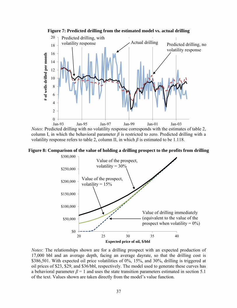
37

Figure 7: Predicted drilling from the estimated model vs. actual drilling

Notes: Predicted drilling with no volatility response corresponds with the estimates of table 2, column I, in which the behavioral parameter β is restricted to zero. Predicted drilling with a volatility response refers to table 2, column II, in which β is estimated to be 1.118.

Figure 8: Comparison of the value of holding a drilling prospect to the profits from drilling

Notes: The relationships shown are for a drilling prospect with an expected production of 17,000 bbl and an average depth, facing an average dayrate, so that the drilling cost is $386,501. With expected oil price volatilities of 0%, 15%, and 30%, drilling is triggered at oil prices of $23, $29, and $36/bbl, respectively. The model used to generate these curves has a behavioral parameter β = 1 and uses the state transition parameters estimated in section 5.1 of the text. Values shown are taken directly from the model’s value function.

0

2

4

6

8

10

12

14

16

18

20

Jan-93 Jan-95 Jan-97 Jan-99 Jan-01 Jan-03

# of

wel

ls d

rill

ed p

er m

onth

$0

$50,000

$100,000

$150,000

$200,000

$250,000

$300,000

20 25 30 35 40

Expected price of oil, $/bbl

Actual drilling Predicted drilling, with volatility response Predicted drilling, no

volatility response

Value of the prospect, volatility = 30%

Value of drilling immediately (equivalent to the value of the prospect when volatility = 0%)

Value of the prospect, volatility = 15%

38

Figure 9: Scatter plot of realized oil production from drilled wells, relative to the number of days required to drill each well

Notes: Production data are from the subset of observed drilled wells that are the only active producing well on their respective lease for the first 36 months subsequent to drilling. This subset amounts to 162 of the observed 1,150 drilled wells from 1993-2003. Dry holes (wells with zero production) are plotted as having a log(production/drilling time) of zero.

0

2

4

6

8

10

12

Jan-93 Jan-95 Jan-97 Jan-99 Jan-01 Jan-03

Log

of

pro

du

ctio

n (

bar

rels

of

oil)

ove

r fi

rst

thre

e ye

ars

of w

ell's

lif

e, m

inu

s lo

g of

d

rilli

ng

tim

e in

day

s

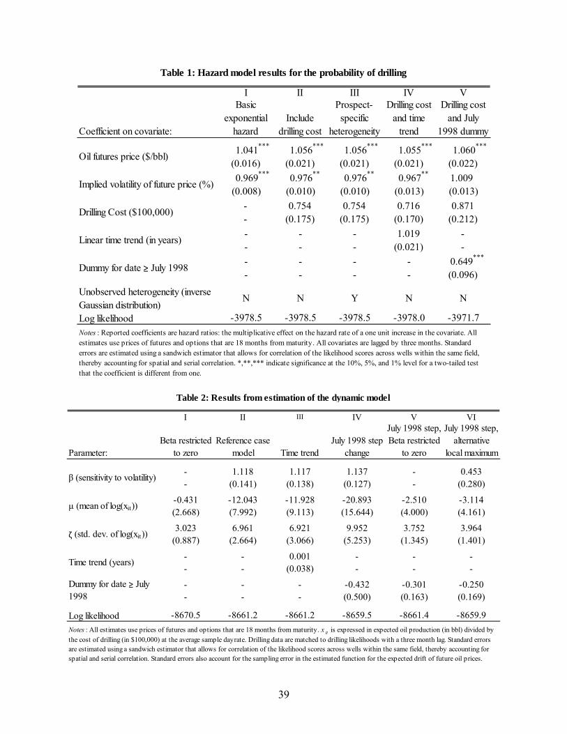
39

I II III IV V

Coefficient on covariate:

Basic exponential

hazardInclude

drilling cost

Prospect-specific

heterogeneity

Drilling cost and time

trend

Drilling cost and July

1998 dummy

1.041*** 1.056*** 1.056*** 1.055*** 1.060***

(0.016) (0.021) (0.021) (0.021) (0.022)

0.969*** 0.976** 0.976** 0.967** 1.009(0.008) (0.010) (0.010) (0.013) (0.013)

- 0.754 0.754 0.716 0.871- (0.175) (0.175) (0.170) (0.212)

- - - 1.019 -- - - (0.021) -

- - - - 0.649***

- - - - (0.096)

Log likelihood -3978.5 -3978.5 -3978.5 -3978.0 -3971.7

Dummy for date ≥ July 1998

Table 1: Hazard model results for the probability of drilling

Oil futures price ($/bbl)

Implied volatility of future price (%)

Drilling Cost ($100,000)

Linear time trend (in years)

N

Notes : Reported coefficients are hazard ratios: the multiplicative effect on the hazard rate of a one unit increase in the covariate. All estimates use prices of futures and options that are 18 months from maturity. All covariates are lagged by three months. Standard errors are estimated using a sandwich estimator that allows for correlation of the likelihood scores across wells within the same field, thereby accounting for spatial and serial correlation. *,**,*** indicate significance at the 10%, 5%, and 1% level for a two-tailed test that the coefficient is different from one.

Unobserved heterogeneity (inverse Gaussian distribution)

N N NY

I II III IV V VI

Parameter:Beta restricted

to zeroReference case

model Time trendJuly 1998 step

change

July 1998 step, Beta restricted

to zero

July 1998 step, alternative

local maximum

- 1.118 1.117 1.137 - 0.453- (0.141) (0.138) (0.127) - (0.280)

-0.431 -12.043 -11.928 -20.893 -2.510 -3.114(2.668) (7.992) (9.113) (15.644) (4.000) (4.161)

3.023 6.961 6.921 9.952 3.752 3.964(0.887) (2.664) (3.066) (5.253) (1.345) (1.401)

- - 0.001 - - -- - (0.038) - - -

- - - -0.432 -0.301 -0.250- - - (0.500) (0.163) (0.169)

Log likelihood -8670.5 -8661.2 -8661.2 -8659.5 -8661.4 -8659.9

Notes : All estimates use prices of futures and options that are 18 months from maturity. x it is expressed in expected oil production (in bbl) divided by

the cost of drilling (in $100,000) at the average sample dayrate. Drilling data are matched to drilling likelihoods with a three month lag. Standard errors are estimated using a sandwich estimator that allows for correlation of the likelihood scores across wells within the same field, thereby accounting for spatial and serial correlation. Standard errors also account for the sampling error in the estimated function for the expected drift of future oil prices.

Table 2: Results from estimation of the dynamic model

Dummy for date ≥ July 1998

β (sensitivity to volatility)

μ (mean of log(xit))

ζ (std. dev. of log(xit))

Time trend (years)

40

Year 1997 1998 1999 2000 2001 2002 2003 2004 2005 2006 2007 2008Employment 4600 5280 4670 4830 5470 5110 5670 7240 7610 7000 8240 10640

Source: Bureau of Labor Statistics, occupation code 19-4041 for 1999-2008 and 22111 for 1997 and 1998

Table 3: Employment of petroleum engineers in Texas

I II III IV V

Parameter:

Reference case model (table 2,

column II)

Historic volatility of futures prices, one year window

GARCH volatility

Mean-reverting volatility

Front month futures and

implied volatility

1.118 0.348 0.587 1.281 1.679(0.141) (0.338) (0.194) (0.157) (0.573)

-12.043 -0.331 -2.481 -9.377 -3.462(7.992) (2.587) (3.552) (6.534) (2.967)

6.961 2.996 3.745 6.092 4.146(2.664) (0.860) (1.188) (2.178) (0.999)

Log likelihood -8661.2 -8670.4 -8666.0 -8661.1 -8662.5

β (sensitivity to volatility)

μ (mean of log(xit))

ζ (std. dev. of log(xit))

Table 4: Alternative specifications of price and volatility beliefs

Notes : x it is expressed in expected oil production (in bbl) divided by the cost of drilling (in $100,000) at the average sample dayrate. Drilling data

are matched to drilling likelihoods with a three month lag. Standard errors are estimated using a sandwich estimator that allows for correlation of the likelihood scores across wells within the same field, thereby accounting for spatial and serial correlation. Standard errors also account for the sampling error in the estimated function for the expected drift of future oil prices.

I II III IV V

Parameter:

Reference case model (table 2,

column II)14.5% nominal discount rate

10.5% nominal discount rate

Rig costs average 20% of total drilling cost

Rig costs average 50% of total drilling cost

1.118 1.189 0.975 1.122 1.127(0.141) (0.176) (0.174) (0.143) (0.133)

-12.043 -10.165 -11.610 -12.869 -13.162(7.992) (7.600) (8.206) (8.544) (7.672)

6.961 6.326 6.823 7.236 7.336(2.664) (2.539) (2.738) (2.847) (2.555)

Log likelihood -8661.2 -8661.5 -8661.3 -8661.9 -8661.0

Table 5: Alternative specifications: discount rates and drilling costs

β (sensitivity to volatility)

μ (mean of log(xit))

ζ (std. dev. of log(xit))

Notes : All estimates use prices of futures and options that are 18 months from maturity. x it is expressed in expected oil production (in bbl)

divided by the cost of drilling (in $100,000) at the average sample dayrate. Drilling data are matched to drilling likelihoods with a three month lag. Standard errors are estimated using a sandwich estimator that allows for correlation of the likelihood scores across wells within the same field, thereby accounting for spatial and serial correlation. Standard errors also account for the sampling error in the estimated function for the expected drift of future oil prices.

A1

APPENDICES TO “THE EFFECT OF UNCERTAINTY ON INVESTMENT:

EVIDENCE FROM TEXAS OIL DRILLING”

Appendix 1: Construction of the time series of implied futures price volatility

This appendix describes how I construct a time series of the implied volatility of 18-

month NYMEX oil futures contracts. As discussed in the main text, I cannot simply use the

Black (1976) formula directly because it assumes that the term structure of volatility (the

function by which the volatility of the future price of oil varies as time to maturity increases) is

constant. My strategy for addressing this issue proceeds in three steps. First, I use the realized

volatility of futures prices to estimate the average term structure of volatility. Second, I use

liquidly traded short-term futures options to generate a time series of the implied volatility of

one-month futures option contracts. Because a one month time horizon is short, this time series is

equivalent to the time series of the implied volatility of one-month futures price contracts.

Finally, I combine the one-month futures price volatilities with the estimated term structure to

generate the desired time series of the implied volatility of 18-month futures price contracts.1

The remainder of this appendix discusses these three steps in turn.

Let Ft,τ denote the price of a NYMEX futures contract traded at date t with time to

maturity τ measured in months.2 For each t and τ, I calculate the realized volatility at t of the τ-

month futures contract as the standard deviation of ln(Fs,τ / Fs-1,τ) for all dates s within the 6

months prior and subsequent to t.3 Let this volatility be denoted by σt,τ. I then estimate the term

structure of futures price volatility by regressing the log of σt,τ on fixed effects for each τ and t:4

ln σt,τ = ητ + δt + ετ,t (A1)

1 An alternative procedure to that used here would use the term structure of the implied volatility of futures options directly to derive the implied volatility of 18-month futures prices. This approach would use the fact that the volatility of a τ-month futures price is equal to the volatility of a τ-month futures option plus τ times the derivative of the futures option term structure (with respect to τ) at τ. The use of the derivative implies that this approach requires a very precise estimate of the term structure of futures options’ implied volatility. Thin markets for futures options beyond 6 months render this procedure impractical. For example, 18-month futures options are traded, on average, only 18 days each year from 1993-2003. 2 Time to maturity in months is equal to the time to maturity in days divided by 365.25, multiplied by 12, and rounded to the nearest whole number. 3 Observations Fs,τ for which date s - 1 is missing (for example, if s - 1 is a Sunday) are excluded. 4 I use the log of σt,τ as the dependent variable rather than the level because the levels regression does not yield an estimated term structure that is stable over time. In levels, the term structure is has a steeper slope during 1999-2003 than in the earlier part of the data.

A2

The fixed effects ητ represent the estimated term structure while the δt control for the

level of volatility on each date t. Given estimates of these fixed effects, the predicted volatility of

a τ-month futures price on date t is given by At·exp(ητ), where At = exp(δt + v2 / 2) and v2 is the

variance of the estimated residuals. Thus, for a fixed trade date t, varying τ will trace out the term

structure of volatility. Figure A2 verifies that the term structure of volatility is stable over the

sample by plotting two estimates of the term structure: one using data from 1999-2003 and

another using data prior to 1999. The constant term A for each plotted estimate is set so that the

one-month future price volatility is 31%, approximately equal to the average one-month

volatility over 1993-2003. The plots overlay each other closely, indicating that the term structure

of volatility is stable over the sample despite the substantial increase in the overall level of

volatility after 1999.

Given the estimated term structure (the ητ), all that is needed to compute expected 18-

month futures price volatilities is a time-series of short-run (one month) expected futures price

volatilities. I derive this time series from the implied volatility of short-term futures options with

a time to maturity between 60 and 180 days. The implied volatility of options with a shorter time

to maturity are noisy, potentially reflecting low option values and integer problems (options

prices must be in whole cents), while options with a longer time to maturity are thinly traded.

For each trade date and time to maturity within the 60 to 180 day window, I use the Black

(1976) model to find the implied volatilities of the call and put options that are nearest to at-the-

money.5 I then estimate the implied volatility term structure by regressing the log of each

option’s implied volatility on its time to maturity τ (in days), a call/put dummy, and trade date

fixed effects δt.6 I then use this estimated term structure (the estimated coefficient on τ) to

extrapolate implied volatility back to a 30 day maturity.

As a validation check on the this procedure, I compare the average, over 1993-2003, of

the estimated implied volatilities of 30-day futures options to the average realized volatility of

one-month futures prices over the same timeframe. These two averages should be approximately

equal given the short one month time to maturity. The former series has an average volatility of

5 The Black (1976) model assumes that the options are European rather than American and that volatility is not stochastic. Neither of these assumptions holds here; however, their effects are likely to be minor and they save considerable computational complexity. Hilliard and Reis (1998) demonstrate that the American premium is no more than 2% of the European option price for volatilities similar to those considered here. Stochastic volatility acts in the opposite direction, causing the Black (1976) model to slightly over-price at-the-money options (this effect is particularly small for the relatively short maturities considered here); see Hull and White (1987), Wiggins (1987), and Poon and Granger (2003). The argument that these assumptions are of minor effect is supported by the close agreement between the average realized and average implied volatility over the 1993-2003 sample. 6 Inspection of the residuals indicates that a linear term structure specification is appropriate. Moreover, when a squared time to maturity term is added, it is not statistically significant (p-value = 0.114).

A3

30.83% while the average of the latter is 31.07%. The closeness of these two numbers (derived

from two completely different data sets) supports the argument that implied volatilities from one-

month futures options can be used as implied volatilities of one-month futures prices.

Finally, I convert the time series of implied volatilities of one-month futures prices to

implied volatilities of 18-month futures prices using the estimated term structure of futures price

volatility (the ητ). This conversion amounts to multiplying the one-month volatility at each trade

date t by exp(η18 - η1).

Appendix 2: Numerical solution and estimation methods

A2.1 Value function iteration

I solve the value function (12) on a grid of points in (P,D,σ,x) space (in logs) using

standard value function iteration. An important factor in defining the grid is that, while the price,

dayrate, and volatility states that are realized in the data are bounded, the stochastic processes for

these variables (equations 4, 5 and 10) imply that agents place nonzero probabilities on

realizations outside of these bounds. Thus, the value function must be solved for states extending

beyond the boundaries of the data. The state space I use extends from one-fifth of the lowest

realized price and dayrate to five times the highest price and dayrate, and from one-half the

lowest realized volatility to twice the highest volatility. With this state space, marginal

reductions or extensions in size do not substantially affect the estimated parameters or the value

function within the range of realized observations.

I found that a relatively dense grid was required to accurately capture the effects of

stochastic volatility. The grid I use has 1,875,000 points: 50 price states by 50 dayrate states by

15 volatility states by 50 productivity states. Starting from this density, the estimated results are

insensitive to increases or decreases in the number of grid points.

In the full estimation routine, the initial value function used for each guess of parameters

is the value function from the previous guess. For the first parameter guess, the initial value

function is zero in all states. The convergence criterion is a tolerance of 10-6 on the sup norm of

the value function (the value function used in the computations is in units of $386,501, the

average drilling cost at the average dayrate). Increasing the tolerance to 10-7 has essentially no

affect on the parameter estimates or value function.

With the value function solved, I can then find, for any given P, D, and σ, the critical

productivity x* such that drilling is optimal iff *ix x . Because the P, D, and σ realizations do

not coincide with the grid states used in the model, I use linear interpolation to find *x . At each

A4

xi grid point, I calculate the value function at the realized P, D, and σ by linearly interpolating the

value function between the states immediately above and below the P, D, and σ. I then find the

smallest xi grid point such that the value of waiting exceeds the realized profits from drilling

immediately and the largest xi such that it is optimal to drill immediately (these two values of xi

will be adjacent grid points). Interpolation gives *x as the productivity level for which the firm is

indifferent: the value of waiting equals the value of drilling immediately. As described in the

text, the realized time series of P, D, and σ can then be combined with a parameterized

distribution on the xit to yield the probability that a given prospect will be drilled each period.

In most of the estimated models, there is no initial conditions problem because the

productivity shocks xit are modeled as iid. An initial conditions problem is present, however, in

the specification allowing for time-invariant prospect heterogeneity (though the specification

ultimately finds no evidence of such heterogeneity). I address this issue by extending the

simulation back to January 1992, so that by 1993, when drilling likelihoods start to be taken, an

equilibrium is approximately reached. This extension requires the interpolation of missing rig

dayrate data for the fourth quarter of 1992.

A2.2 Estimation

I search for the parameters β, μ, and log ζ that maximize the log-likelihood function (13)

via a gradient-based search that uses the BFGS method for computing the Hessian at each step (I

take the logarithm of ζ to allow for negative values in the parameter search). I accelerate the

search by conducting it in two stages. First, holding β fixed, I search for the μ and log ζ that

maximize the likelihood. This stage is fast because changing μ and ζ does not require re-solving

the model. The outer-most loop then searches for β. The stopping criterion is a tolerance on the

likelihood function (scaled down by a factor of 10,000) of 10-10 for the μ and ζ loop and 10-8 for

the β loop.

To compute the standard errors of the parameter estimates, I obtain the likelihood score

of each observation (drilling prospect - month) numerically. With respect to each parameter θk, I

calculate the derivative of the log likelihood for observation j as ( ) ( )

2j k k j k k

k

θ ε θ ε

ε

l l. For the

parameters β and μ, I use a value for εk of 0.001, and for log ζ I use a value of 0.0001 because the

likelihood function is particularly concave in this parameter. The standard errors are robust to

values of εk that are an order of magnitude larger or smaller.

A5

I adjust the standard errors to account for the fact that the parameters of the expected

price drift function (11) are estimated in a first stage.7 Denoting the first-stage parameters (κp0,

κp1, and κp2) and log-likelihood function by θ1 and L1, and denoting the second-stage parameters

(β, μ, and ζ) and log-likelihood function by θ2 and L2, I apply the procedure of Murphy and Topel

(1985) using equation (A2),

1 1 ' 1 1

2 2 3 1 3 2R R R R R R (A2)

where Σ denotes the corrected variance-covariance matrix for θ2, and

'

1 11

'

2 2 22

21

1 '1 1 1 1

2

2 '2

2

'1 1 2

2 2 2

'

2 2 23

2

( )

( )

( )

L L LR E E

L L LR E E

L L LR E E

(A3)

R1 is simply the inverse of the variance-covariance matrix from the least-squares estimate

of the price drift function (11), which I compute using standard errors clustered on month-of-

sample.8 R2 is the inverse of the unadjusted (and non-clustered) second-stage variance-

covariance matrix. Calculation of R3 requires numerical derivatives of the second-stage

likelihood function with respect to the first-stage parameters. I calculate these derivatives in the

same way that I calculate those with respect to the second stage parameters, as discussed above.

The perturbations I use for κp0, κp1, and κp2 are 10-5, 10-6, and 10-3, respectively.

For the specifications that yield estimates of β near one, the above procedure roughly

increases the estimated standard errors by a factor of 3, a magnitude similar to that found in

several examples in Murphy and Topel (1985). The adjustment is not substantial for other

specifications, however, as their unadjusted standard errors are already large.

7 The volatility of volatility (γ), the ratio of dayrate volatility to oil price volatility (α), and the correlation between dayrate and price shocks (ρ) are also estimated in a first stage. However, I found that these parameters contributed only negligibly to the standard errors of the main parameter estimates in the reference case model. To reduce computational burden, the results presented in the paper therefore ignore these parameters when computing Murphy and Topel two-step standard errors. 8 Clustering on year rather than month-of-sample does not substantially affect the estimated standard errors.

A6

Figure A1: Infill drilling in sole operated vs. all fields

Figure A2: Estimated term structures of futures price volatility

Notes: The figure displays two term structures, one estimated using data from before 1999, the other using data from 1999-2003. Volatility of a one-month future is set to 31.0% for both term structures.

0

50

100

150

200

250

300

0

2

4

6

8

10

12

14

16

18

20

Jan-93 Jan-95 Jan-97 Jan-99 Jan-01 Jan-03

Wel

ls p

er m

onth

, all

fie

lds

Wel

ls p

er m

onth

, un

itiz

ed f

ield

s

0

5

10

15

20

25

30

35

0 3 6 9 12 15 18

Vol

atili

ty (

%, a

nn

ual

)

Time to maturity in months

pre-1999

1999 - 2003

All infill wells Infill wells in sole-operated fields