the effect of wastewater treatment plant effluent on water

The Effect of Wastewater Treatment Plant Effluent on Water Temperature, Macroinvertebrate Community, and Functional Feeding Groups Structure in the Lower

Rouge River, Michigan

by

Esma Tuncay

A thesis submitted in partial fulfillment of the requirements for the degree of

Master of Science (Environmental Science)

in the University of Michigan-Dearborn 2016

Master’s Thesis Committee: Professor Larissa L. Sano, University of Michigan, Co-Chair Professor Orin Gelderloos, Co-Chair Professor Sonia M. Tiquia-Arashiro Sally Petrella, Friends of the Rouge

ii

DEDICATION

I dedicate this Master’s thesis to my husband Joel Deussen who has encouraged me and supported

me through the whole research process. He is the pillar of my life and gave me the strength for

perseverance and determination.

I also dedicate this thesis to my parents Selma and Hidayet Tuncay and my siblings Fatma and

Ahmet in Germany. Even though, we are separated by the Atlantic Ocean and a vast distance, they

always were at my side and supported me.

Thanks to all for their huge support.

Istanbul, 9 Dec 2016.

iii

ACKNOWLEDGMENTS

First, I would like to thank my thesis advisor Larissa Sano, PhD of the College of Literature,

Science, and the Arts at the University of Michigan. Prof. Sano was always available when I had

questions regarding my research and writing and guided me in the whole research process.

Additionally, I would like to thank her for help during the summer sampling of macroinvertebrates

for my research and providing all the necessary equipment for my research.

I would also thank Orin Gelderloos, PhD of the Natural Science Department at the University of

Michigan-Dearborn. The door to Prof. Gelderloos office was always open for additional questions

regarding my thesis. I am grateful for his very valuable comments and guidance throughout the

thesis process.

I would also like to acknowledge Sonia M. Tiquia-Arashiro of the Natural Science Department at

the University of Michigan-Dearborn and Sally Petrella from Friends of the Rouge as the thesis

committee member for their expertise and I am gratefully indebted to both of them for their very

valuable comments on this thesis.

Finally, I would like to thank Robert Muller and Philip Kukulski for designing the PVC

temperature sensor holders. I would like to thank Robert Muller for building the PVC temperature

sensor holders, for helping me setting the temperature sensors and regularly checking on them. I

also thank all the volunteers at Friends of the Rouge and Wayne County Department of Public

Works Water Quality Management Division, especially Susan Thompson for helping me sample

and picking the sampled macroinvertebrates from trays for identification.

iv

Additionally, I would like to thank 4th Street Auto located at 303 E. Fourth Street in Royal Oak,

MI. 48067 for donating the break discs which were used to weigh down the temperature sensors

and secure them at place.

Thank you,

Esma Tuncay

v

TABLE OF CONTENTS DEDICATION ................................................................................................................................ ii ACKNOWLEDGMENTS ............................................................................................................. iii LIST OF TABLES ....................................................................................................................... viii LIST OF FIGURES ...................................................................................................................... xii LIST OF APPENDICES .............................................................................................................. xvi LIST OF ABBREVIATIONS ..................................................................................................... xvii ABSTRACT ................................................................................................................................. xix CHAPTER I .................................................................................................................................... 1 1. INTRODUCTION ................................................................................................................... 1

1.1. Thermal regime of streams and rivers .............................................................................. 1 1.1.1. Factors influencing the thermal regime of streams and rivers .................................. 2 1.1.2. Thermal regime heat exchange processes ................................................................. 3 1.1.3. Longitudinal water temperature variation of streams and rivers .............................. 4 1.1.4. Annual and daily variation of thermal regime .......................................................... 4 1.1.5. Analyzing thermal regime ......................................................................................... 5

1.1.5.1. Scaling area of study .......................................................................................... 5 1.1.5.2. Water temperature of streams and rivers ........................................................... 6

1.1.6. Influence of water temperature on aquatic fauna ...................................................... 6 1.2. Thermal discharge and thermal pollution......................................................................... 8

1.2.1. Anthropogenic influences on thermal regime ........................................................... 8 1.2.2. History of thermal discharge ..................................................................................... 9 1.2.3. Thermal discharge properties .................................................................................. 10 1.2.4. The effects of thermal discharges on thermal regime ............................................. 11

1.2.4.1. Thermal regime ................................................................................................ 11 1.2.4.2. Effects of thermal discharge on aquatic animals ............................................. 12 1.2.4.3. Other effects of thermal discharges ................................................................. 13

1.2.5. Previous research on thermal discharges ................................................................ 13 1.2.5.1. Thermal discharge and its effects on macroinvertebrates ............................... 13 1.2.5.2. Longitudinal effects of thermal discharges on macroinvertebrates ................. 16 1.2.5.3. Thermal discharge and their effects on functional feeding groups ................. 16

1.2.6. Future research ........................................................................................................ 17 1.3. Benthic macroinvertebrates ............................................................................................ 17 1.3.1. Habitat ............................................................................................................................ 18

1.3.2. Functional feeding groups....................................................................................... 18 1.4. Study area: Lower Rouge River ..................................................................................... 20

1.4.1. Problem statement ................................................................................................... 22 1.4.2. Pollution in the Rouge River................................................................................... 23

1.5. Wastewater treatment plant in Ypsilanti ........................................................................ 24 1.6. Research focus................................................................................................................ 30

CHAPTER II ................................................................................................................................. 35

vi

2. MATERIALS AND METHODS .......................................................................................... 35 2.1 Sampling locations ......................................................................................................... 35 2.2 Air and water temperature determination....................................................................... 37

2.1.1. Air temperature ....................................................................................................... 37 2.1.2. Water temperature ................................................................................................... 37

2.3. Discharge rate from waste water treatment plant and the Inkster, MI gauge ................. 39 2.4. Benthic macroinvertebrate sampling and analysis ......................................................... 41

2.4.1. Macroinvertebrate sampling time periods .............................................................. 42 2.4.2. Macroinvertebrate sampling method ...................................................................... 43 2.4.3. Macroinvertebrate analysis ..................................................................................... 44 2.4.4. Historical comparison ............................................................................................. 44

2.5. Statistical analyses.......................................................................................................... 45 2.5.1. Temperature ............................................................................................................ 45 2.5.2. Macroinvertebrate statistical analyses .................................................................... 46

CHAPTER III ............................................................................................................................... 49 3. RESULTS .............................................................................................................................. 49

3.1. Water temperature .......................................................................................................... 49 3.1.1. Mean daily water temperature by seasons .............................................................. 49

3.1.1.1. Spring............................................................................................................... 49 3.1.1.2. Summer ............................................................................................................ 52 3.1.1.3. Fall ................................................................................................................... 55

3.1.2. Comparison of water temperatures by sites ............................................................ 58 3.1.3. Covariance and Correlation .................................................................................... 60

3.1.3.1. Spring............................................................................................................... 60 3.1.3.2. Summer ............................................................................................................... 63

3.1.3.3. Fall ................................................................................................................... 65 3.1.4. Wastewater treatment plant discharge and the Inkster USGS gauge discharge ..... 67

3.1.4.1. Spring............................................................................................................... 67 3.1.4.2. Summer ............................................................................................................ 68 3.1.4.3. Fall ................................................................................................................... 69

3.2. Macroinvertebrates ......................................................................................................... 70 3.2.1. Macroinvertebrate species diversity and habitat quality ......................................... 70

3.2.1.1. Spring............................................................................................................... 71 3.2.1.1.1. Comparison of Fowl2 and Outfall (LR-2) ................................................... 71 3.2.1.1.2. Comparison of downstream locations and the Outfall ................................ 72 3.2.1.1.3. Comparison of downstream locations and Fowl2 ....................................... 74

3.2.1.2. Summer ............................................................................................................ 76 3.2.1.2.1. Comparison of Fowl2 with the Outfall (LR-2) ............................................ 76 3.2.1.2.2. Comparison of the Outfall with downstream locations ............................... 77 3.2.1.2.3. Comparison of Fowl2 with downstream locations ...................................... 77

3.2.1.3. Fall ................................................................................................................... 80 3.2.1.3.1. Comparison of Fowl2 and Outfall (LR-2) ................................................... 80 3.2.1.3.2. Comparison of Outfall with downstream locations ..................................... 81 3.2.1.3.3. Comparison of Fowl2 with downstream locations ...................................... 82

3.2.2. Functional feeding groups....................................................................................... 85 3.2.2.1. Spring............................................................................................................... 85

vii

3.2.2.2. Summer ............................................................................................................ 88 3.2.2.3. Fall ................................................................................................................... 90

CHAPTER IV ............................................................................................................................... 92 4. DISCUSSION ........................................................................................................................ 92

4.1. Thermal regime .............................................................................................................. 92 4.1.1. Temperature ............................................................................................................ 92

4.2. Macroinvertebrates ......................................................................................................... 98 4.2.1. Functional feeding groups..................................................................................... 103

4.3. Conclusion .................................................................................................................... 105 4.4. Future research ............................................................................................................. 106

BIBLIOGRAPHY ....................................................................................................................... 128

viii

LIST OF TABLES

Table 1. Effluent regulation by MDEQ (YCUA). ___________________________________ 27

Table 2. Water temperature at the Lower Rouge River on November 14th, 2014 (Data from FOTR). ____________________________________________________________________ 28

Table 3. Water temperature sensor and sample locations on the Lower Rouge River. Fowl2 is the control site. _________________________________________________________________ 35

Table 4. Mean temperature (mean T) in °C and standard deviation (STDEV) with maximum and minimum average water temperature for spring from 13 April to 15 June 2015. Temperatures mean was calculated from mean daily water temperatures from spring. LR-2 is the Outfall. __ 50

Table 5. Mean temperature (mean T) in °C and standard deviation (STDEV) with maximum and minimum average water temperature for summer from 16 June to 31 August 2015. Temperature mean was calculated from mean daily water temperatures from summer. LR-2 is the Outfall. 53

Table 6. Mean temperature (mean T) in °C and standard deviation (STDEV) with maximum and minimum average water temperature for fall from 1 September to 26 October 2015. Temperature mean was calculated from mean daily water temperatures from fall. LR-2 is the Outfall. ____ 56

Table 7. The daily mean water temperature of each location was tested on normal distribution by using skewness and kurtosis for the seasons spring (13 April to 15 June), summer (16 June to 31 August), and fall (1 September to 26 October) in 2015. Reported are the z-values for skewness and kurtosis. The normal distribution applies for absolute z-values below 3.29 for sample size between 50 and 300. Sample size for spring was 64, for summer was 77, and for fall was 56._ 58

Table 8. Mean water temperature (T) in °C and standard deviation (STDEV) for all locations from April through October. ____________________________________________________ 59

Table 9. Independent Student’s t-test with equal variance for the locations Fowl2 and Outfall for each season. The t-tests were calculated from the mean daily temperatures of Fowl2 and the Outfall. P-values below 0.05 are considered significantly different. * p < 0.05, ** p < 0.01, *** p < 0.001 ____________________________________________________________________ 59

Table 10. P-values for the independent Student’s t-test with equal variances comparing Fowl2 with the downstream locations LR-12, LR-6, and LR-10 for spring, summer, and fall 2015. P-values below 0.05 are considered significantly different. ______________________________ 60

ix

Table 11. P-values for the independent Student’s t-test with equal variances comparing Fowl2 and the Outfall with the downstream locations LR-12, LR-6, and LR-10 for spring, summer, and fall 2015. P-values below 0.05 are considered significantly different. ____________________ 60

Table 12. Covariance and correlation coefficient of mean daily water and air temperatures in °C for the locations Fowl2/Outfall, Fowl2/LR-12, Fowl2/LR-6, Fowl2/LR-10, Outfall/LR-12, Outfall/LR-6, Outfall/LR-10, Air/Fowl2, Air/Outfall, Air/LR-12, Air/LR-6, and Air/LR-10 for spring (13 April – 15 June 2015). ________________________________________________ 61

Table 13. Covariance and correlation coefficient of mean daily water temperatures in °C for the locations Fowl2/Outfall, Fowl2/LR-12, Fowl2/LR-6, Fowl2/LR-10, Outfall/LR-12, Outfall/LR-6, Outfall/LR-10, Air/Fowl2, Air/Outfall, Air/LR-12, Air/LR-6, and Air/LR-10 for summer (16 June– 31 August 2015). _______________________________________________________ 63

Table 14. Covariance and correlation coefficient of mean daily water temperatures in °C for the locations Fowl2/Outfall, Fowl2/LR-12, Fowl2/LR-6, Fowl2/LR-10, Outfall/LR-12, Outfall/LR-6, Outfall/LR-10 Air/Fowl2, Air/Outfall, Air/LR-12, Air/LR-6, and Air/LR-10 for fall (1 September– 26 October 2015). __________________________________________________ 65

Table 15. Percentage (%) and number of individuals (#) in each family of macroinvertebrates in spring calculated by the raw data. Macroinvertebrates are categorized to sensitive, somewhat sensitive, and tolerant groups (Michigan Clean Water Corps). The number (N) of family taxa is the number of families at each location. LR-2 is the Outfall. ___________________________ 75

Table 16. Shannon diversity index and Shannon’s Evenness in spring for each location. LR-2 is the Outfall. _________________________________________________________________ 76

Table 17. Bray-Curtis Index for spring. The Bray-Curtis Index shows the percentage similarity in macroinvertebrate community between the two locations Fowl2/LR-2, Fowl2/LR-12, Fowl2/LR-6, Fowl2/LR-10, LR-2/LR-12, LR-2/LR-6, and LR-2/LR-10. LR-2 is the Outfall. _ 76

Table 18. Percentage (%) and number of individuals (#) in each family of macroinvertebrates in summer calculated by the raw data. Macroinvertebrates are categorized to sensitive, somewhat sensitive, and tolerant groups (Michigan Clean Water Corps). The number (N) of family taxa is the number of families at each location. LR-2 is the Outfall. ___________________________ 79

Table 19. Shannon diversity index and Shannon’s Evenness in summer for each location. LR-2 is the Outfall. ________________________________________________________________ 80

Table 20. Bray-Curtis Index for summer. The Bray-Curtis Index shows the percentage similarity in macroinvertebrate community between the two locations Fowl2/LR-2, Fowl2/LR-12, Fowl2/LR-6, Fowl2/LR-10, LR-2/LR-12, LR-2/LR-6, and LR-2/LR-10. LR-2 is the Outfall. _ 80

Table 21. Percentage (%) and number of individuals (#) in each family of macroinvertebrates in fall calculated by the raw data. Macroinvertebrates are categorized to sensitive, somewhat sensitive, and tolerant groups (Michigan Clean Water Corps). The number (N) of family taxa is the number of families at each location. LR-2 is the Outfall. ___________________________ 84

x

Table 22. Shannon diversity index and Shannon’s Evenness in fall for each location. LR-2 is the Outfall. ____________________________________________________________________ 85

Table 23. Bray-Curtis Index for fall. The Bray-Curtis Index shows the percentage similarity in macroinvertebrate community between the two locations Fowl2/LR-2, Fowl2/LR-12, Fowl2/LR-6, Fowl2/LR-10, LR-2/LR-12, LR-2/LR-6, and LR-2/LR-10. LR-2 is the Outfall. __________ 85

Table 24. The Bray-Curtis Index was determined to compare the percentage similarity of functional feeding groups individuals of Fowl2 to the Outfall, LR-12, LR-6, LR-10 and Outfall to LR-12, LR-6, and LR-10 for spring 2015. _______________________________________ 87

Table 25. Shannon diversity index and Shannon’s evenness for the functional feeding groups at each location during spring 2015. ________________________________________________ 87

Table 26. The Bray-Curtis Index was determined to compare the percentage similarity of functional feeding groups individuals of Fowl2 to the Outfall, LR-12, LR-6, LR-10 and Outfall to LR-12, LR-6, and LR-10 for summer 2015. ______________________________________ 89

Table 27. Shannon diversity index and Shannon’s evenness for the functional feeding groups at each location during summer 2015. ______________________________________________ 89

Table 28. The Bray-Curtis Index was determined to compare the percentage similarity of functional feeding groups individuals of Fowl2 to the Outfall, LR-12, LR-6, LR-10 and Outfall to LR-12, LR-6, and LR-10 for fall 2015. _________________________________________ 91

Table 29. Shannon diversity index and Shannon’s evenness for the functional feeding groups at each location during fall 2015. __________________________________________________ 91

Table 30. Mean water temperature difference between the control site Fowl2 and the sites LR-2, LR-12, LR-6, and LR-10 for the three seasons spring, summer, and fall 2015. ____________ 111

Table 31. Mean water temperature difference between the Outfall and the downstream sites LR-12, LR-6, and LR-10 for the three seasons spring, summer, and fall 2015. _______________ 112

Table 32. Past spring benthic macroinvertebrate data for Fowl2 2012 to 2015 from FOTR. R means rare (1-10) and C means common (>10).____________________________________ 118

Table 33. Past spring benthic macroinvertebrate data for the Outfall 2014 to 2015 from FOTR. R means rare (1-10) and C means common (>10).____________________________________ 119

Table 34. Past spring benthic macroinvertebrate data for LR-12 2012 to 2015 from FOTR. R means rare (1-10) and C means common (>10).____________________________________ 120



xi

Table 37. Past fall benthic macroinvertebrate data for Fowl2 2012 to 2015 from FOTR. R means rare (1-10) and C means common (>10). _________________________________________ 123

Table 38. Past fall benthic macroinvertebrate data for LR-2 2012 to 2015 from FOTR. R means rare (1-10) and C means common (>10). _________________________________________ 124


Table 40. Past fall benthic macroinvertebrate data for LR-6 2012 to 2015 from FOTR. Fall 2014 was not sampled. R means rare (1-10) and C means common (>10). ___________________ 126


xii

LIST OF FIGURES

Figure 1. Factors influencing the thermal regime of rivers (Caissie 2006). ________________ 3

Figure 2. Mean daily and diel variability of water temperatures as a function of stream order/downstream direction (Caissie 2006). _________________________________________ 5

Figure 3. Comparison of thermal requirements of carp (Cyprinus carpio) and brown trout (Salmon trutta) (Langford 1990). _________________________________________________ 7

Figure 4. The Rouge River watershedwith its four major branches the Main, Upper, Middle and Lower. The four major branches are also divided into the seven subwatersheds Main 1-2, main 3-4, Upper, Middle 1, Middle 3, Lower 1, and Lower 2 (LOSAG 2001a). __________________ 21

Figure 5. The Lower Rouge River and its two subwatershed Lower 1 and 2 (LOSAG 2001a). 22

Figure 6. Water temperature in the Lower Rouge River on November 14th, 2014. The discharge is located at LR-2 with 16.06 ˚C and the lower temperature 2.1 are recorded upstream of the discharge at Fowl2. LR-12, LR-6, and LR-10 showed higher temperature than Fowl2 which are downstream of LR-2 (Courtesy from FOTR and Robert Muller). _______________________ 29

Figure 7. Median daily water temperatures at the Lower Rouge River between 2013 and 2015 measured by the USGS gauge 04168400 at Dearborn, MI. Daily mean water temperature for the year 2014 was statistically determined. (http://nwis.waterdata.usgs.gov/nwis/uv?cb_00010=on&format=gif_stats&site_no=04168400&period=&begin_date=2013-01-01&end_date=2015-11-23). Data from November 23th. ______ 32

Figure 8. Sampling and temperature sensor locations on the Lower Rouge River. Temperature sensors were installed at Fowl2, LR-2, LR-12, LR-6, and LR-10. _______________________ 36

Figure 9. A drawing to visualize how the temperature sensor was placed in the river. Red is the PVS casing with the temperature sensor inside and black is the break rotor to stretch the chain in order to have the temperature sensor in the water column. ____________________________ 38

Figure 10. Robert Muller holding the PVC casing with the temperature sensor inside and the break rotor. _________________________________________________________________ 39

Figure 11. US Geological Survey (USGS 2015) 04168000 gauge at Jeffrey Lane in Inkster, MI.___________________________________________________________________________ 40

Figure 12. Discharge rate in cubic feet per second at USGS gauge 04168000 Inskter, MI from March to October 2015 (USGS 2016). ____________________________________________ 43

xiii

Figure 13. Mean daily water and air temperatures for spring measured in ˚C from 13 April to 15 June 2015. The water temperature was measured hourly and averaged for a 24-hour period. The mean daily air temperature was calculated from daily maximum and minimum air temperatures. The top graph shows all the following temperatures. A) Fowl2, B) LR-2, C) LR-12, D) LR-6, E) LR-10 and F) air._____________________________________________________________ 51

Figure 14. Mean daily water and air temperatures for spring measured in ˚C from 16 June to 31 August 2015. The water temperature was measured hourly and averaged for a 24-hour period. The mean daily air temperature was calculated from daily maximum and minimum air temperatures. The top graph shows all the following temperatures. A) Fowl2, B) LR-2, C) LR-12, D) LR-6, E) LR-10 and F) air. _______________________________________________ 54

Figure 15. Mean daily water and air temperatures for spring measured in ˚C from 1 September to 26 October 2015. The water temperature was measured hourly and averaged for a 24-hour period. The mean daily air temperature was calculated from daily maximum and minimum air temperatures. The top graph shows all the following temperatures. A) Fowl2, B) LR-2, C) LR-12, D) LR-6, E) LR-10 and F) air. _______________________________________________ 57

Figure 16. Correlation of mean daily water temperatures (°C) of the following locations: A) Fowl2/Outfall (LR-2), B) Fowl2/LR-12, C) Fowl2/LR-6 D) Fowl2/LR-10, E) Outfall (LR-2)/LR-12, F) Outfall (LR-2)/ LR-6, and G) Outfall/LR-10 for spring (April – 15 June 2015). _ 62

Figure 17. Correlation of mean daily water temperatures in °C of the following locations: A) Fowl2/Outfall (LR-2), B) Fowl2/LR-12, C) Fowl2/LR-6 D) Fowl2/LR-10, E) Outfall (LR-2)/LR-12, F) Outfall (LR-2)/ LR-6, and G) Outfall/LR-10 for summer (16 June – 31 August 2015). _____________________________________________________________________ 64

Figure 18. Correlation of mean daily water temperatures in °C of the following locations: A) Fowl2/Outfall (LR-2), B) Fowl2/LR-12, C) Fowl2/LR-6 D) Fowl2/LR-10 E) Outfall (LR-2)/LR-12 F) Outfall (LR-2)/ LR-6 G) Outfall/LR-10 for fall (1 September – 26 October 2015). ____ 66

Figure 19. Daily discharge rate from the wastewater treatment plant (WWTP) and Inkster, MI USGS gauge during spring (13 April -15 June 2015). Discharge rates for the WWTP were converted from million of gallons per day into cubic meter per second (m3/sec). The daily discharge rate at Inkster, MI was calculated by USGS based on measurements made each 15 minutes (USGS 2016) in cft/sec and was converted to m3/sec. _________________________ 68

Figure 20. Daily discharge rate from the wastewater treatment plant (WWTP) and Inkster, MI USGS gauge during summer (16 June – 13 August 2015).). Discharge rates for the WWTP were converted from million of gallons per day into cubic meter per second (m3/sec). The daily discharge rate at Inkster, MI was calculated by USGS based on measurements made each 15 minutes (USGS 2016) in cft/sec and was converted to m3/sec. _________________________ 69

Figure 21. Daily discharge rate from the wastewater treatment plant (WWTP) and the Inkster, MI USGS gauge during fall (1 September – 26 October 2015). Discharge rates for the WWTP were converted from million of gallons per day into cubic meter per second (m3/sec). The daily discharge rate at Inkster, MI was calculated by USGS based on measurements made each 15 minutes (USGS 2016) in cft/sec and was converted to m3/sec. _________________________ 70

xiv

Figure 22. Numbers of individuals of functional feeding groups in spring. Collector-gatherers (c-g), collector-filterers (c-f), shredders (shr), scrapers (scr), engulfer-predators (engulfer-prd), and piercer-predators (piercer-(prd). LR-2 is the Outfall. _________________________________ 87

Figure 23. Numbers of individuals of functional feeding groups in summer. Collector-gatherers (c-g), collector-filterers (c-f), shredders (shr), scrapers (scr), engulfer-predators (engulfer-prd), and piercer-predators (piercer-(prd). ______________________________________________ 89

Figure 24. Numbers of individuals of functional feeding groups in fall. Collector-gatherers (c-g), collector-filterers (c-f), shredders (shr), scrapers (scr), engulfer-predators (engulfer-prd), and piercer-predators (piercer-(prd). Y-axis was changed to logarithmic scale for a better visualization. ________________________________________________________________ 91

Figure 25. Mean daily water and air temperature for April 2015 calculated from the raw 24 hourly measured water temperature data. _________________________________________ 107

Figure 26. Mean daily and air water temperature for May 2015 calculated from the raw 24 hourly measured water temperature data. _________________________________________ 108

Figure 27. Mean daily and air water temperature for June 2015 calculated from the raw 24 hourly measured water temperature data. _________________________________________ 108

Figure 28. Mean daily water and air temperature for July 2015 calculated from the raw 24 hourly measured water temperature data. _________________________________________ 109

Figure 29. Mean daily water and air temperature for August 2015 calculated from the raw 24 hourly measured water temperature data. _________________________________________ 109

Figure 30. Mean daily water and air temperature for September 2015 calculated from the raw 24 hourly measured water temperature data. _________________________________________ 110

Figure 31. Mean daily water and air temperature for October 2015 calculated from the raw 24 hourly measured water temperature data. _________________________________________ 110

Figure 32. Discharge rate in cubic meter per second (m3/sec) for the Outfall and Inkster USGS gauge from April to October 2015. ______________________________________________ 113

Figure 33. Discharge rate in cubic meter per second (m3/sec) for the Outfall and Inkster USGS gauge in April 2015. _________________________________________________________ 114

Figure 34. Discharge rate in cubic meter per second (m3/sec) for the Outfall and Inkster USGS gauge in May 2015.__________________________________________________________ 115

Figure 35. Discharge rate in cubic meter per second (m3/sec) for the Outfall and Inkster USGS gauge in June 2015.__________________________________________________________ 115

Figure 36. Discharge rate in cubic meter per second (m3/sec) for the Outfall and Inkster USGS gauge in July 2015. __________________________________________________________ 116

xv

Figure 37. Discharge rate in cubic meter per second (m3/sec) for the Outfall and Inkster USGS gauge in August 2015. _______________________________________________________ 116

Figure 38. Discharge rate in cubic meter per second (m3/sec) for the Outfall and Inkster USGS gauge in September 2015. _____________________________________________________ 117

Figure 39. Discharge rate in cubic meter per second (m3/sec) for the Outfall and Inkster USGS gauge in October 2015. _______________________________________________________ 117

xvi

LIST OF APPENDICES

APPENDIX 1 Monthly mean daily water and air temperature from April to October 2015 ............................. 107

APPENDIX 2 Mean water temperature difference between the control site and LR-2, LR-12, LR-6, and LR-10..................................................................................................................................................... 111

APPENDIX 3 Mean water temperature difference between the Outfall and LR-12, LR-6, and LR-10 ............ 112

APPENDIX 4 Discharge rate at the Outfall and at the Lower Rouge River in Inkster, MI from April to October..................................................................................................................................................... 113

APPENDIX 5 Monthly discharge rate at the Outfall and at the Lower Rouge River in Inkster, MI ................. 114

APPENDIX 6 Past data of macroinvertebrate families for each location from 2012 to 2015 for spring and fall..................................................................................................................................................... 118

xvii

LIST OF ABBREVIATIONS

CPOM Coarse particulate organic matter

FPOM Fine particulate organic matter

DOM Dissolved organic matter

AOC Area of Concern

YCUA Ypsilanti Community Utilities Authority

NPDES National Pollutant Discharge Elimination System

WWTP wastewater treatment plant

WTUA Western Township Utilities Authority

ML/d million liters per day

Mgd million gallons per day

MDNR Michigan Department of Natural Resources

MDEQ Michigan Department of Environmental Quality

CBOD5 Carbonaceous biochemical oxygen demand

N Nitrogen

FOTR Friends of the Rouge

NOAA National Oceanic and Atmospheric Administration

xviii

USGS United States Geological Survey

stdev Standard deviation

m3/sec Cubic meter per sec

cft/sec Cubic feet per sec

xix

ABSTRACT

The release of effluent from wastewater treatment plants can impact receiving water bodies by

altering water temperatures. The Ypsilanti Community Utilities Authority (YCUA) has been

discharging its wastewater effluent into the Lower Rouge River since 1996. To understand the

impact of these discharges on water temperature in the Rouge River, this study measured the water

temperature hourly from April 13 to October 26, 2015 at five different locations: one at the

discharge site (LR-2), three below the effluent discharge (LR-12, LR-6, and LR-10), and one

upstream of the discharge (Fowl2, control site) at the Lower Rouge River, MI. Additionally,

benthic macroinvertebrates were sampled during spring, summer, and fall to analyze the impacts

of changes in water temperatures on the macroinvertebrate fauna. Water temperatures at the

discharge site (LR-2) showed significantly different temperatures than the upstream control site

(Fowl2) during summer 2015. The sites further downstream significantly differed in water

temperature compared to LR-2 during summer 2015 for LR-12, LR-6, and LR-10 and during fall

2015 for LR-12 and LR-6. However, water temperature at the Lower Rouge River below the

YCUA discharge did not contribute to changes in macroinvertebrate family richness and diversity.

Additionally, functional feeding groups were analyzed. Fowl2 had higher numbers of the

functional feeding group collector-gatherers compared to collector-filterers, which suggests that

the fine organic particulate matter (FOPM) is distributed on the river bottom. Yet, the functional

feeding group collector-filterer were higher below the YCUA discharge compared to Fowl2, which

indicates a shift in FOPM from the river bottom into the water column which could be caused by

the YCUA discharge flow. My results suggest that the YCUA discharge temperature did not have

xx

any influence on the downstream sites LR-12, LR-6, and LR-10. Additionally, different family

richness and diversity of macroinvertebrates are most likely caused by a shift in nutrient

distribution (FPOM) rather than a change in water temperature.

1

CHAPTER I

1. INTRODUCTION

Urban watersheds are water catchment areas of waterbodies in urban areas. They have

multiple stressors on the watershed affecting the watersheds biological, chemical, and physical

conditions resulting from urbanization compared to rural watersheds. They are characterized by

impervious surfaces created through residential and commercial structures, as well as roads. For

certain reasons such as flooding control, infrastructural issues, or water transport, the river is

shaped, straightened, concrete channeled or closed underground to fit municipal planning. The

natural shape of the watershed is lost and subject to many anthropogenic influences. Point and

non-point source pollution result in biological and chemical pollution. In addition, impervious

surfaces result in higher surface run-off which increases the river discharge rapidly and result in

extreme river bank erosion and flooding. Thermal pollution can also occur through municipal or

industrial discharges into the river which can change the natural water temperature and affect the

aquatic ecosystem (Caissie 2006). The Rouge River watershed in Michigan, USA is an example

of an urban watershed.

1.1.Thermal regime of streams and rivers

The thermal regime of a river reflects the daily and annual water temperature variation in

a watershed. These fluctuations affect the quality and health of the aquatic ecosystem and stream

productivity (Caissie 2006; Verones et al. 2010) because water temperature is an important abiotic

2

factor, which influences biochemical and physiological activities of aquatic organisms (Verones

et al. 2010). Temperature is a physical factor that can also influence chemical reactions, the

properties of chemicals, and microbial activity (Dallas 2008).

1.1.1. Factors influencing the thermal regime of streams and rivers

The thermal regime of a river is influenced by atmospheric conditions, topography, stream

discharge, and streambed (Caissie 2006; Dallas 2008). Atmospheric conditions such as solar

radiation, air temperature, cloud cover, vapor pressure, wind speed, humidity, precipitation,

evaporation, condensation, and phase changes of water which are responsible for heat exchange

processes at the water surface (Caissie 2006; Dallas 2008). Upland shading, riparian vegetation,

geology, stream orientation, channel form, slope, water depth, turbidity, percentage of pool habitat,

as well as latitude and altitude define the topographical and structural influences on the thermal

regime of rivers surface (Caissie 2006; Dallas 2008). Therefore, topography also determines the

intensity of the influences of atmospheric conditions on the thermal regime, for example high

canopy cover during spring and summer reduces the input of solar radiation to the stream and

therefore protects the stream from getting too warm for some fauna and flora (Caissie 2006).

Stream discharge determines the volume of water based on inflow and outflow (Caissie 2006). The

heat capacity of river water depends on the amount of water and the mixing by turbulence, slopes,

waterfalls, and friction on the streambed (Caissie 2006). The streambed is important for

groundwater input and hyporheic exchange, which is also important for the volume of water and

the heat exchange capacity (Figure 1).

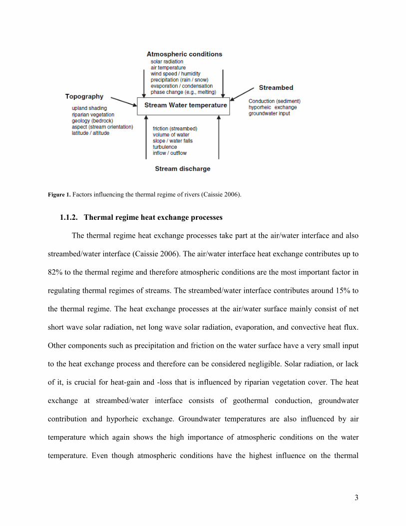
3

Figure 1. Factors influencing the thermal regime of rivers (Caissie 2006).

1.1.2. Thermal regime heat exchange processes

The thermal regime heat exchange processes take part at the air/water interface and also

streambed/water interface (Caissie 2006). The air/water interface heat exchange contributes up to

82% to the thermal regime and therefore atmospheric conditions are the most important factor in

regulating thermal regimes of streams. The streambed/water interface contributes around 15% to

the thermal regime. The heat exchange processes at the air/water surface mainly consist of net

short wave solar radiation, net long wave solar radiation, evaporation, and convective heat flux.

Other components such as precipitation and friction on the water surface have a very small input

to the heat exchange process and therefore can be considered negligible. Solar radiation, or lack

of it, is crucial for heat-gain and -loss that is influenced by riparian vegetation cover. The heat

exchange at streambed/water interface consists of geothermal conduction, groundwater

contribution and hyporheic exchange. Groundwater temperatures are also influenced by air

temperature which again shows the high importance of atmospheric conditions on the water

temperature. Even though atmospheric conditions have the highest influence on the thermal

4

regime, riparian vegetation and the size of the river must be considered in determining the

influence of the different heat exchange processes.

1.1.3. Longitudinal water temperature variation of streams and rivers

Streams and rivers begin as small tributaries at the headwater. They increase in size and

water volume in downstream direction as they connect with other tributaries. The downstream

direction or river length from the headwaters to the mouth is called the longitudinal direction of

streams and rivers. Water temperature at the source of a river is close to groundwater temperature

and increases both in a longitudinal direction from headwaters to the mouth with increasing stream

order (Caissie 2006; Vannote and Sweeney 1980). Small streams usually increase 0.6 °C per km,

intermediate streams increase 0.2 °C per km, and larger rivers increase 0.09 °C per km (Caissie

2006). Therefore, water temperatures changes with river size, but temperature change is usually

non-linear and depends on many factors (Caissie 2006). Different habitat types such as pool, run,

and riffle habitats show small scale temperature variation because they differ in size, depth and

stream velocity (Dallas 2008; Vannote and Sweeney 1980). Also, different types of rivers and

streams have different thermal regimes (Caissie 2006). For example, braided rivers have small and

shallow channels that are prone to faster temperature changes.

1.1.4. Annual and daily variation of thermal regime

In temperate areas, the thermal regimes of streams vary both daily and seasonally (Caissie

2006; Dallas 2008). Daily minimum temperature is reached at sunrise and daily maximum

temperature is reached in the late afternoon and early evening (Caissie 2006; Dallas 2008). Daily

water temperature fluctuations vary with location, whereas headwater streams show the lowest

temperature fluctuation due to the influence of groundwater sources (Caissie 2006; Vannote and

Sweeney 1980). In a downstream direction, rivers are more affected by atmospheric conditions

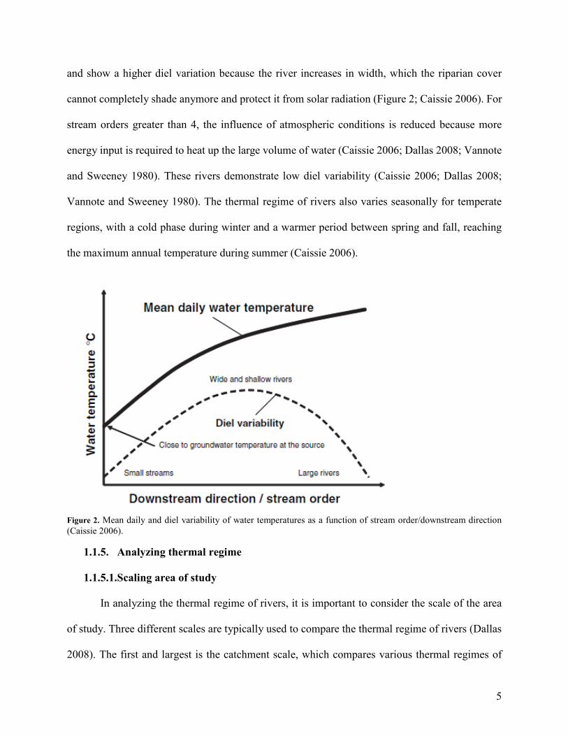
5

and show a higher diel variation because the river increases in width, which the riparian cover

cannot completely shade anymore and protect it from solar radiation (Figure 2; Caissie 2006). For

stream orders greater than 4, the influence of atmospheric conditions is reduced because more

energy input is required to heat up the large volume of water (Caissie 2006; Dallas 2008; Vannote

and Sweeney 1980). These rivers demonstrate low diel variability (Caissie 2006; Dallas 2008;

Vannote and Sweeney 1980). The thermal regime of rivers also varies seasonally for temperate

regions, with a cold phase during winter and a warmer period between spring and fall, reaching

the maximum annual temperature during summer (Caissie 2006).

Figure 2. Mean daily and diel variability of water temperatures as a function of stream order/downstream direction (Caissie 2006).

1.1.5. Analyzing thermal regime

1.1.5.1.Scaling area of study

In analyzing the thermal regime of rivers, it is important to consider the scale of the area

of study. Three different scales are typically used to compare the thermal regime of rivers (Dallas

2008). The first and largest is the catchment scale, which compares various thermal regimes of

6

individual rivers with each other, thereby accounting for the change in climate, geography,

topography, and vegetation (Dallas 2008). The second scale is at the river level, which compares

the thermal regime within a river system (Dallas 2008). Analysis at the river scale focuses on water

temperature changes longitudinally from the headwaters to the mouth (Dallas 2008, Figure 2).

Water temperatures usually increase in a downstream direction and reach maximum values in the

middle reaches (Dallas 2008). The third scale is the site scale, which compares the thermal regime

of a small section of a river with different habitat that consists of different depths and therefore

different water temperatures (Dallas 2008; Langford 1990).

1.1.5.2.Water temperature of streams and rivers

The thermal regime of lotic waterbodies can be divided into water column temperature,

water and streambed substrate interface temperature, and substrate temperature (Langford 1990).

Most aquatic animals live at the water and streambed substrate interface (Langford 1990). At the

water and streambed substrate interface the temperature is generally the same as that of the water

column (Langford 1990).

1.1.6. Influence of water temperature on aquatic fauna

Many aquatic animals require a specific temperature range for optimal distribution, growth,

reproduction, and fitness (Caissie 2006; Dallas 2008; Vannote and Sweeney 1980). The optimal

temperature range for aquatic fauna is defined as the temperature that leads to maximum body

weight and fecundity without causing physiological stress (Vannote and Sweeney 1980). It differs

between organisms (Vannote and Sweeney 1980). For example, the carp (Cyprinus carpio) grows

best at temperatures between 23 - 29 ˚C whereas the brown trout (Salmon trutta) requires lower

temperature between 7 - 17 ̊ C for optimal growth (Figure 3). Macroinvertebrates also have optimal

water temperature preference such as 9.1 – 10.6 °C for Drunella cryptomenria, 10.3 – 11.6 °C for

7

Stenelmis sp., and 10.8 – 12 °C for Asellus sp. (Li et al. 2013). However, most freshwater

macroinvertebrates reach thermal death for water temperatures between 30 to 40°C (Wallace and

Anderson 1996). In general, aquatic fauna are more sensitive to high temperature than aquatic flora

(Verones et al. 2010).

Figure 3. Comparison of thermal requirements of carp (Cyprinus carpio) and brown trout (Salmon trutta) (Langford 1990).

Aquatic animals are ectothermic organisms and therefore water temperature can have a

direct effect on their growth, development, respiration, excretion, and general fitness (Dallas 2008;

De Stasio, Golemgeski, and Livingstone 2009). Because of their sensitivity to water temperature,

water temperature can affect their abundance and diversity (Dallas 2008; Vannote and Sweeney

1980). Temperature is also a physical factor that can influence other chemical reactions, the

properties of chemicals, and microbial activity (Dallas 2008). For instance, the toxicity of

chemicals increases with increasing temperature (e.g. Ammonia increases in toxicity by a factor

of 1.3 to 1.6 in relation to pH for temperature increases from 10°C to 20°C) (Cairns, Heath, and

8

Parker 1975) while the dissolved oxygen concentration decreases with higher temperatures (e.g.

Concentration of O2 (mg/L) in pure water at 0°C is 14.2 mg/L and at 30°C is 7.5 mg/L) (Allan and

Castillo 2007a). With higher water temperature, the metabolic activity of aquatic animals increases

as well, which leads to faster depletion of dissolved oxygen concentration and lower food resources

(Dallas 2008). Thus spatial and temporal changes in water temperature influences the behavior of

aquatic animals and therefore are important factors to understanding the responses of aquatic fauna

to water temperature changes (Dallas 2008).

According to the river continuum concept (Vannote et al. 1980), daily and seasonal stream

water temperature variation is responsible for the distribution of aquatic animals (Caissie 2006).

Fishes are able to detect temperature changes of 0.05 ˚C and their neuronal system selects the

optimal growth temperature (Langford 1990). Fish thus tend to avoid waters around thermal

discharge sites and move to water with a temperature closer to their optimal growth temperature

(Langford 1990). Benthic macroinvertebrates are also impacted by temperature. They show higher

drifting rates with higher temperatures and therefore avoid the thermal discharge by moving

downstream (Langford 1990). Individual species show different tolerance to temperature and the

movement rate will vary from species to species (Langford 1990). Li et al. (2013) researched the

distribution of macroinvertebrates species according to different water temperatures in South

Korean streams. In their study, the most sensitive taxa to increasing water temperature were

Ephemeroptera, Plecoptera, and Trichoptera (Li et al. 2013).

1.2.Thermal discharge and thermal pollution

1.2.1. Anthropogenic influences on thermal regime

Thermal discharges generate a point source of water with an elevated temperature into a

receiving waterbody (Gooch 2007). Thermal discharges can be divided into natural and artificial

9

ones. Geothermal discharges such as geysers and hot springs are natural and discharge their hot

waters (up to 100°C) to adjacent lentic and lotic habitats (Langford 1990). These hot temperatures

support a unique flora and fauna for these areas (Langford 1983). Artificial thermal discharges

results from anthropogenic activities that affect the thermal regime of lotic ecosystems both

directly and indirectly (Dallas 2008). The magnitude of direct and indirect effects on thermal

regimes can vary in regard to the river water volume and geographical location of the river. Rivers

and streams can be affected by a variety of point- and non-point sources, which can have a

cumulative effect on the change of their thermal regime (Poole, Risley, and Hicks 2001).

Artificial thermal discharges range from point to non-point sources. Thermal discharges

from power plants, industrial processes, municipal waste water treatment plants, air conditioning

and refrigerator plants, impoundments and dams are classified as point source discharges because

they are discharged directly to the waterbody next to their location (Langford 1990). The most

prominent thermal discharges come from power plants and may show higher water temperatures

(up to 42°C) (Coutant 1962) than the other discharge types and, therefore, could have a larger

influence on thermal regimes over a section of streams and rivers (Langford 1990).

Non-point sources are often scattered around the watershed. These non-point sources range

from impervious surface run-off to agricultural drainage (Dallas 2008; Langford 1990; Schueler

1994). Other activities such as afforestation and deforestation, change of riparian vegetation, and

global warming can change the water temperature as well (Dallas 2008; Langford 1990). The

degree of effects depends on the number of point and non-point sources (Langford 1983).

1.2.2. History of thermal discharge

Humans start using water for cooling purposes since ancient time. Historically, thermal

10

discharge became more prevalent and larger with human activities during the Industrial Revolution

which resulted in mass production and increased the usage of water for cooling purposes (Langford

1990). Factories were built adjacent to waterbodies in order to use the water for cooling processes.

This water was then discharged back to the waterbody after use. This large amount of thermal

discharge can change the thermal regime of receiving waterbodies and affect their aquatic

ecosystem (Dallas 2008; Langford 1990).

Some of the first concerns about the ecological effects of thermal discharge arose from

exotic snails appearing in cooling ponds for steam engines (Langford 1990). These snails (Menetus

dilatatus) were first discovered in cooling ponds in Manchester, UK in 1869, having been

introduced from North America (Macan 1960). The “Electricity Act of 1919” in the United

Kingdom noted that thermal discharges may have an effect on the aquatic ecosystem and the

“Ministry of Health” of the United Kingdom noted in 1949 that 1°C could have an adverse effect

on the aquatic ecosystem (Langford 1990). But the first public awareness of thermal discharges as

thermal pollution and their effects on the native aquatic ecosystem arose in 1952 from the lawsuit

against the Spondon Power Station. Many studies focused on the effects of thermal discharges on

the aquatic ecosystem from the mid-1950s to the 1960s and started the “thermal pollution era”.

Research concerning thermal discharges began to decline in the late 1970s, even though the

amount of thermal discharges continued to increase.

1.2.3. Thermal discharge properties

Thermal discharges can be divided into rapid jet discharges, which have a higher

turbulence and mixing rate with the receiving water, and low turbulence and velocity discharges,

which usually go into the top layer of the receiving waters (Langford 1990). Thermal discharge

has the ability to change the thermal regime of rivers by increasing the water temperature and flow

11

regime of these waterbodies. Changes in flow regime may lead to change in direction and velocity

and therefore in sediment deposition. In addition, warm water has a lower density and higher

buoyancy, which can change the density and buoyancy properties of the receiving water.

1.2.4. The effects of thermal discharges on thermal regime

1.2.4.1.Thermal regime

The effects of thermal discharges on the receiving waterbodies usually depends on the size,

volume of water, water depth, rate of mixing, and velocity of the receiving waters as well as on

the volume of discharged water (Langford 1990). Therefore, smaller receiving rivers will be more

affected than larger ones (Vannote and Sweeney 1980). In addition, in temperate regions, the

seasonal variation of lotic water temperatures further determines the effect of the thermal discharge

on the thermal regime (Caissie 2006) because the temperature of thermal discharge also fluctuates

with seasons (Dallas 2008; Langford 1990). Temperature fluctuations of thermal discharges can

lead to unstable thermal regime of the receiving waters, but an unstable thermal regime of receiving

streams could be stabilized by stable thermal discharges (Langford 1990). The impact area of the

thermal discharge depends on the channel width and depth of the stream. Thermal discharge

usually mixes well with small streams, but large rivers could concentrate the effect of the thermal

discharge on a narrow path of flow along on the bank at the discharge and lead to lateral

stratification of the river. Usually, thermal discharges are transported downstream, but during low

flow and high upstream wind periods, the discharge could be transported a small distance

upstream. The high upstream wind periods could move the thermal discharge over a short distance

upstream during low flow periods and also alter the thermal regime in the immediate upstream

region.

12

1.2.4.2.Effects of thermal discharge on aquatic animals

The effects of temperature on aquatic animals can be either lethal or sub-lethal (Langford

1990). Lethal temperatures are temperatures that are high enough to cause direct death to the

animal (Caissie 2006; Langford 1990). Sub-lethal temperatures are temperatures that do not

directly kill an individual, but that can cause changes in behavior such as movement and migration

and can impact physiological and biochemical processes such as higher metabolic activity and

respiration and/or impairments in growth and reproduction (Langford 1990). Metabolic activity

increases with temperature and reaches a maximum level, which is followed by death (Langford

1990; Verones et al. 2010; Voshell 2002). Van’t Hoff’s rule implies a doubling in metabolic

activity with every 10 °C increase in water temperature (Caissie 2006; Dallas 2008). Therefore,

increased metabolic activity leads to indirect effects resulting in oxygen depletion (Caissie 2006).

Other indirect effects of thermal discharges are the change in chemical toxicity and a higher

demand of food (Caissie 2006; Langford 1990). The increase in metabolic activity of aquatic

animals’ result in a higher demand of food. The higher demand for food will in turn have an effect

on predators, competitors, and prey and therefore could change the trophic level composition

(Dallas 2008; Langford 1990). The impaired metabolic activity can also lead to impaired

reproduction (Verones et al. 2010) which will result in lower off spring and less competition

(Vannote and Sweeney 1980). Other sub-lethal effects can influence growth (Hogg et al. 1995;

Hogg and Williams 1996), behavior, food and feeding habitats (Dallas 2008), life history (Hogg

and Williams 1996), geographical distribution (Li et al. 2013), community structure (Li et al.

2013), movements (Durrett and Pearson 1975), migration (Durrett and Pearson 1975), and the

tolerance to parasites, diseases and other pollution (Dallas 2008). Therefore, a single impairment

has the ability to cause a chain reaction of other effects that can have impacts on the individual

13

species, and at subpopulation, population, and community levels. Lethal and sub-lethal

temperatures are specific to each species, but in general the tolerance to temperature changes is

higher in physiologically and morphologically less complex taxa (Langford 1990).

1.2.4.3.Other effects of thermal discharges

Thermal discharges can also influence the chemical properties of water such as dissolved

oxygen concentrations as well as the toxicity of chemicals (Caissie 2006; Dallas 2008; Langford

1990). Dissolved oxygen concentration are inversely related to water temperature and decreases

with increasing water temperatures (Caissie 2006; Dallas 2008; Langford 1990). However, high

velocity and mixing rate can create turbulence that mitigates the effect of the thermal discharge on

dissolved oxygen concentrations (Langford 1990). On the other hand, the toxicity of chemicals

increases with higher temperatures (Langford 1990). Chlorine is one of the chemicals that is added

to the thermal discharge to prevent biological fouling of pipes and culverts (Langford 1983) and

is the main culprit for impaired aquatic ecology rather than temperature alone (Langford 1990).

1.2.5. Previous research on thermal discharges

Most studies of the effects of thermal discharges on river ecology are from power plant

releases and generally were conducted between the 1960s and the 1980s ( Langford and Aston

1972; Osborne and Davies 1987; Alston et al. 1978; Benda and Proffitt 1974; Coutant 1962;

Howell and Gentry 1974; Massengill 1976; LeRoy Poff and Matthews 1986; Wurtz and Skinner

1984). Studies from the 1990s shifted to focus on climate warming and its effect on the

macroinvertebrate fauna (Hogg and Williams 1996; Hogg et al. 1995), but research on thermal

discharges continued (Wellborn and Robinson 1996; Worthington et al. 2015).

1.2.5.1.Thermal discharge and its effects on macroinvertebrates

Coutant (1962) is one of the earliest researcher to analyze the effects of thermal discharge

14

on macroinvertebrate fauna in riffle habitats. Several subsequent studies found that thermal

discharge has the most deleterious effect during summer months, with water temperature ranging

between 40 and 42 °C causing decreases in the abundance of macroinvertebrates (Coutant 1962;

Durrett and Pearson 1975; Wellborn and Robinson 1996). Sensitive taxa such as Trichoptera,

Ephemeroptera and Plecoptera occurred in lower numbers and demonstrated lower species

diversity in thermally disturbed areas (Howell and Gentry 1974; Li et al. 2013), whereas tolerant

taxa dominated these areas including Chironomidae (Benda and Proffitt 1974; Coutant 1962;

Coutant and Brook 1970; Howell and Gentry 1974) and Oligochaeta (Osborne and Davies 1987).

Unlike these other studies, elevated water temperatures in winter were associated with an increase

of up to 10 to 40 % in benthic fauna biomass (Coutant and Brook 1970). In contrast to the other

studies, Langford (1972) reported no significant negative effects associated with thermal

discharges in British rivers. Therefore, a generalized assumption about the effects of thermal

discharge on macroinvertebrates fauna is not possible.

Other studies compared the effects of thermal discharges on invertebrate fauna with

considering the chemical pollution level of the river. Langford and Aston (1972) compared a

chemical polluted and non-polluted river receiving thermal discharge in Britain. The water

temperature was measured below the outfall between 1965 to 1970 for the non-polluted river and

between 1965 to 1966 for the polluted river. The maximum water temperature below the thermal

discharge was up to 6°C above average in the non-polluted river and 10°C above average in the

polluted river. Neither river showed any difference in their upstream and downstream fauna

diversity of invertebrates. The non-polluted river consisted of many diverse invertebrate taxa with

many intolerant species, however, in comparison, the polluted river had low diversity. The polluted

river showed lower macroinvertebrate diversity mainly due to the chemical pollution from

15

domestic and industrial effluents because macroinvertebrate diversity was drastically reduced at

River Trent below the confluence with the highly chemically polluted River Tame. There were

differences between rivers in terms of life history of certain species, specifically the Oligochaete

community. They showed a shift towards the species Limnodrilus hoffmeisteri with a peak cocoon

production in October below the discharge of the polluted river compared to May for population

in the upstream reaches. Also, below the outfall in non-polluted reaches, the species Heptagenia

sulphurea emerged earlier, which show that the life history of some species seems to be affected

by higher water temperature. However, Hogg and Williams (1996) observed faster adult

emergence and faster growth of some species due to moderate high water temperatures of 2°C in

spring, summer and fall, and 3.5°C in winter. In the higher temperature sites, some species also

showed smaller size at maturity and altered sex ratios in comparison to thermally non-affected

areas. These finding indicate that the effects of thermal pollution can have different effects on

species in terms of life history.

Thermal discharges do not always result in high elevated water temperatures in the

receiving waterbodies and macroinvertebrates show different behavior compared to higher water

temperature increases. Regarding moderate water temperature increases, studies have reported

different outcome in macroinvertebrates in comparison to higher elevated water temperatures.

LeRoy Poff and Matthews (1986) observed an increase in macroinvertebrate abundance and taxa

at the confluence site of the stream with the Savannah River in North Carolina which was slightly

thermally effected. Dahlberg and Conyers (1974) also observed an increase in taxa and individual

numbers during winter for water temperatures between 9.5 and 17 °C. However, Hogg et al. (1995)

observed a decrease in total density of benthic macroinvertebrates with an average increase of 2°C

in spring, summer and fall, and 3.5°C in winter. Therefore, a general assumption about the fate of

16

macroinvertebrate fauna for moderate water temperature increases is not possible.

1.2.5.2.Longitudinal effects of thermal discharges on macroinvertebrates

Thermal discharge effects are often limited to the immediate downstream areas (Coulter et

al. 2014; Osborne and Davies 1987). For example, Worthington et al. (2015) measured 4.5 °C

elevated water temperatures 2 km downstream of a power station outfall. However, abundance and

taxa richness were only affected at sites 0.5 km downstream of the outfall. There were no

significant changes in the benthic macroinvertebrate community greater than 2 km downstream.

Similarly, Massengill (1976) observed a recovery of benthic fauna approximately 1 km below the

discharge. Benda and Proffitt (1974) observed effects on benthic macroinvertebrate abundance and

taxa diversity 152 m to 274 m below the discharge, which was on average 6 °C higher than control

stations.

1.2.5.3.Thermal discharge and their effects on functional feeding groups

Few studies have researched the effects of thermal discharge on the functional feeding

groups (functional feeding groups are described in detail in section 1.3.2) of benthic

macroinvertebrates. LeRoy Poff and Matthews (1986) was the only study that reported the effects

of thermal discharge on the response of functional feeding groups. They reported a change in

functional feeding groups from collector-gatherers at control areas to scrapers at thermally-

affected areas. However, areas affected only moderately by thermal release showed a different

response with a change in community composition from collector-gatherers to collector-filterers

(LeRoy Poff and Matthews 1986). These data were collected over a 48-day period during winter

and did not provide information for other seasons. Given this, it appears that additional research is

needed to understand effects of thermal discharges on the functional feeding groups of benthic

macroinvertebrates at different seasons.

17

1.2.6. Future research

One opportunity for future research is to measure the long-term stream temperatures in

relation to macroinvertebrate fauna. Most of the previously cited studies did not describe

temperature measurement methods and lacked detail in terms of temperature reporting such as how

frequently and with what instruments they measured the water temperature (Benda and Proffitt

1974; Coutant 1962; Dahlberg and Conyers 1974; Langford and Aston 1972; Massengill 1976;

LeRoy Poff and Matthews 1986; Wellborn and Robinson 1996; Wurtz and Skinner 1984). Also,

some researchers reported that water temperature was just measured during macroinvertebrate

sampling (Coutant 1962) or measured once a month (Osborne and Davies 1987). This lack of daily

water temperature reporting over the study time frame makes it difficult to relate water temperature

with macroinvertebrate fauna and therefore can miss short term pulses of water temperature, which

can eliminate all fauna. Therefore, a more detailed analysis regarding temperature measurements

would help to compare different research outcomes for long-term studies. In addition, research

regarding thermal discharge and their effects on functional feeding groups is limited in the

literature and future research is needed to assess if impairments in the stream food-web are caused

by thermal discharge.

1.3.Benthic macroinvertebrates

Benthic macroinvertebrates are aquatic animals that includes aquatic insects, clams, snails,

worms, and crayfish (USEPA 1997). These organisms are used for biological monitoring in

streams to assess long- and short-term effects of certain pollutants and to determine the habitat and

water quality of the stream (Nedeau, Merritt, and Kaufman 2003; USEPA 1997).

Macroinvertebrates are considered a useful way of monitoring biological conditions in a stream

because they cannot escape pollution due to their limited mobility (Nedeau, Merritt, and Kaufman

18

2003; USEPA 1997). Thus, they are good biological indicators of long-term chemical, physical,

and biological pollution. Different orders of macroinvertebrates show different tolerance to

pollution and are classified into sensitive, somewhat sensitive, and tolerant taxonomic orders

(MCWC 2005). Macroinvertebrates also play an important part in nutrient cycling, primary

production, decomposition, and translocation (Wallace and Webster 1996) and are therefore food

sources for numerous fish species and important in the stream-food web (USEPA 1997; Wallace

and Webster 1996). Macroinvertebrates link many trophic levels. Therefore, impairments on

macroinvertebrates could have both a top-down and a bottom-up effect on the food chain because

they are consumers at the intermediate trophic level (Wallace and Webster 1996). Given their

importance in the food web, changes in the thermal regime could lead to a reduction in size of

macroinvertebrates with low fecundity and therefore lower their ability to compete (Vannote and

Sweeney 1980).

1.3.1. Habitat

Benthic macroinvertebrates are found in all types of stream habitat such as riffles, runs,

pools, and undercut banks, but usually prefer slow water habitats (Hershey et al. 2010).

Macroinvertebrates live mostly at and in the water-streambed substrate interface (Hershey et al.

2010; Voshell 2002). They are also found on submerged wood and leaf packages. The substrate

they inhabit can be organic or inorganic (Hershey et al. 2010). Organic substrates consist of leaf

material and wood, while inorganic substrates range from silty sediments to boulders (Hershey et

al. 2010).

1.3.2. Functional feeding groups

Most macroinvertebrates consume a range of foods including wood, algae, live vascular

plants, detritus, and other animals (Voshell 2002). Because they have specific ways of obtaining

19

food, they are divided into functional feeding groups (Huryn 2009; Voshell 2002). The functional

feeding groups include shredders, scrapers (grazers), collectors, engulfing predators, and piercers

(Hershey et al. 2010; Huryn 2009; Voshell 2002). Shredders, scrapers, collectors, and piercer-

herbivores are plant material eating macroinvertebrates (Voshell 2002). Engulfing-predator and

piercer-predator macroinvertebrates are carnivores (Voshell 2002).

Shredders consume coarse particulate organic matter (CPOM) resulting from decomposing

terrestrial litter and living macrophyte tissue (Hershey et al. 2010; Wallace and Webster 1996).

They use COPM to produce fine particulate organic matter (FPOM) and dissolved organic matter

(DOM), which is food for other macroinvertebrates (Huryn 2009; Wallace and Webster 1996).

Grazers or scrapers feed on microbial biofilms attached to substrate including periphyton, diatoms,

and other heterotrophic prokaryotes and eukaryotes (Hershey et al. 2010; Huryn 2009). They

scrape the biofilm from the substrate surface (Wallace and Webster 1996). Grazer and algae

abundance are interrelated and a lack in grazer population can lead to an increase of algae and is

another example of macroinvertebrates having a top-down effect on the trophic level (Wallace and

Webster 1996). Collectors are subdivided into collector-gatherers and collector-filterers (Huryn

2009). Collector-gatherers feed on FPOM on the streambed and collector-filterers feed on FPOM

suspended in the water column (Huryn 2009). Piercers are divided into piercer-herbivores and

piercer-predators (Voshell 2002). Piercer-herbivores feed on plant fluid by penetrating the plant

tissue (Voshell 2002). Piercer-predators feed on animal fluids by sucking the fluids out of their

prey (Voshell 2002). Their prey are usually larger than the predators and consist mostly of other

invertebrates, although some can also prey on vertebrates such as fish and tadpoles (Voshell 2002).

Engulfing predators eat living animals and forage on benthic and water-column habitat (Hershey

et al. 2010; Huryn 2009).

20

1.4.Study area: Lower Rouge River

The Rouge River is a small urban watershed of up to 1210 km2 catchment area with 203

km of stream (LOSAG 2001a; LTSAG 2001a). It is located in Southeast Michigan and a tributary

to the Detroit River. The watershed encompasses the Washtenaw, Wayne, and Oakland Counties

and contains 48 communities with 1.5 million residences (Figure 4). The Rouge River is divided

into the four major branches: Main, Upper, Middle, and Lower Branch. The four major branches

are divided into seven subwatersheds. The main branch consists of the subwatersheds Main 1-2

and 3-4, the Middle Branch of Middle 1 and 3, and the Lower Branch of Lower 1 and 2. As much

as 50 % of the urbanization in the Rouge River watershed is concentrated along the Lower 2 and

Main Branch in Dearborn, Melvindale, and Inkster (LTSAG 2001a). The undeveloped areas are

concentrated more in rural areas at the east and southeast part of the Lower 1 and east part of the

Middle 1 Branch such as Salem, Superior, and Van Buren (Figure 4, LOSAG 2001b).

The Rouge River suffered significantly from pollution and degradation in the past. Because

of that, the Rouge River is a designated Area of Concern (AOC) and governed by management

plans to improve water and habitat quality, such as the Rouge River Remedial Action Plan and

seven subwatershed management plans (LTSAG 2001a).

The focus of this study is the Lower Branch of the Rouge River (Figure 4 and Figure 5).

The Lower Branch is the most southerly branch of the Rouge River with a 246 km2 catchment

area, separated into Lower 1 and 2 subwatersheds, and shared by Washtenaw and Wayne counties

(Figure 4, LOSAG 2001b; LTSAG 2001b).

21

Figure 4. The Rouge River watershedwith its four major branches the Main, Upper, Middle and Lower. The four major branches are also divided into the seven subwatersheds Main 1-2, main 3-4, Upper, Middle 1, Middle 3, Lower 1, and Lower 2 (LOSAG 2001a).

22

Figure 5. The Lower Rouge River and its two subwatershed Lower 1 and 2 (LOSAG 2001a).

1.4.1. Problem statement

The Lower Rouge River watershed suffered significantly from low baseflow conditions

before 1996, especially during summer months (LOSAG 2001b; LTSAG 2001b; Wiley, Seelbach,

and Bowler 1998). This resulted in lowest daily average flow ranging from 0.03 to 0.06 m3

(LTSAG 2001b; LOSAG 2001b; Wiley, Seelbach, and Bowler 1998). The low stream discharge

rate led to nearly zero dissolved oxygen concentrations and dramatically decreased habitat quality

(LOSAG 2001b; LTSAG 2001b). In 1996, the Ypsilanti Community Utilities Authority (YCUA)

wastewater treatment plant started to discharge wastewater effluent into the Lower Rouge at Beck

Rd in Canton, MI (LTSAG 2001b; LOSAG 2001b). The stream discharge increased to 0.71 m3 for

the lowest daily average and increased dissolved oxygen concentration to up to 7 mg/l (LTSAG

2001b). The effluent discharge improved the flow regime and dissolved oxygen concentrations on

the Lower Rouge River, but it could also serve as a source of pollution (LTSAG 2001b) by altering

the thermal regime of the river.

23

1.4.2. Pollution in the Rouge River

Chemical and bacterial pollution in the Rouge River is highly prevalent due to the heavy

industry adjacent to the watershed and the combined sewer overflows. Heavy metal contamination

of the river bed is common in the Rouge River due to the industrial activities of over 100 years

along the river (Murray et al. 1999) which are more prevalent at the soil surface at industrial sites

close to the east side of the watershed (Murray, Rogers, and Kaufman 2004). Additionally, Murray

et al. (1999) found out that the concentration of heavy metal in sediment particles increases with

smaller particle size. Kannan et al. (2001) identified several organic pollutants in the sediments of

the Lower Rouge such as polychlorinated naphthalene, biphenyl, dibenzo-p-dioxins,

dibenzofurans and polycyclic aromatic hydrocarbons which were most likely caused by combined

sewer outflow and industrial facilities along the river. Additionally, the impact of organic pollution

on heterotrophic microbial communities is reflected in higher metabolic diversity (Tiquia 2011)

and enzyme activities (Tiquia 2010). Another potential source of pollution into the Lower Rouge

River are bacterial pollution coming from domesticated animal and wildlife runoff (Murray et al.

2001). Furthermore, Tiquia et al. (2007) found a shift towards halophilic and halotolerant bacteria

communities resulting from the runoff of deicing salts into the Rouge River.

Previous studies on the Rouge River concentrated mainly on chemical and bacterial

pollution, whereas Wayne County Michigan conducted research on the water temperature in the

Rouge River. Wayne County recorded continuous temperatures from 1994 to 2005 at 8 locations

in the Rouge River (Price 2014). From 2007 to 2012, continuous temperature measurements were

taken at a minimum of one location within the Rouge River watershed (Price 2014). Temperatures

at the Lower Rouge River were continuously measured from 1994 to 2005 at Hannan Rd (US9) in

Wayne, MI and Military Ave. (L05D) in Dearborn, MI (Price 2014). Other continuous water

24

temperature measuring stations are the USGS Gauge 041684001 (Dearborn, MI), USGS gauge

041665002 (Detroit, MI), and USGS gauge 041671503 (Dearborn Heights, MI).

There are a few sites in the Rouge River that are potential source of thermal pollution. The

Main Branch receives thermal discharge from AK Steel in Dearborn before it drains into the

Detroit River4. AK Steel is required to conduct a thermal plume study over four seasons for spring

(March through June), summer (July through August), fall (September through November), and

winter (December through February) for the recent National Pollutant Discharge Elimination

System (NPDES) permit. The thermal plume study started in 2015 and concluded in August 2016.

The study included four discharge locations and determined the temporal, spatial, thermal and

volumetric characteristics of the thermal plume, and provided the volume, velocity, time of

passage and time-temperature information in the intake facilities, in the discharge facilities, and in

the centerline of the thermal plume.

1.5.Wastewater treatment plant in Ypsilanti

The wastewater treatment plant (WWTP) is located in southeast Ypsilanti, Michigan. The

plant is owned and operated by the YCUA. YCUA provides wastewater treatment for the City of

Ypsilanti, Ypsilanti Township, Augusta Township, Pittsfield Township, Sumpter Township,

Superior Township, York Township, Canton Township, Northville, and Plymouth (YCUA 2012b).

The last three communities are members of Western Township Utilities Authority (WTUA) in

Wayne County which agreed with YCUA to expand the YCUA facility to be able to receive

1 http://waterdata.usgs.gov/mi/nwis/uv/?site_no=04168400&PARAmeter_cd=00065,00060 2 http://waterdata.usgs.gov/mi/nwis/uv/?site_no=04166500&PARAmeter_cd=00065,00060 3 http://waterdata.usgs.gov/mi/nwis/uv/?site_no=04167150&PARAmeter_cd=00065,00060 4 Information from Sally Petrella (FOTR).

25

sewage from these communities (YCUA 2012b). In addition, YCUA collects wastewater from the

City of Ypsilanti and Ypsilanti Township (YCUA 2012b).

YCUA began operating in 1982, serving all the communities listed above except the

WTUA (YCUA 2016). The WWTP was designed for an average daily discharge of 109.4 million

liters per day (ML/d) (28.9 million gallons per day (mgd)) (YCUA 2012a). Initially, all of this

treated wastewater was discharged to Willow Creek, adjacent to the WWTP and part of the Huron

River Watershed. In 1988, the wastewater from the WTUA was added to YCUA. Because of this,

a new discharge permit from the Michigan Department of Natural Resources (MDNR) was

attained for an average flow of 219.6 ML/d (58 mgd). This resulted in the creation of an additional

outfall into the Lower Rouge River. The permit was approved to allow discharge to the Lower

Rouge River in order to prevent more nutrient loading into the Bellville Lake (YCUA 2012a;

YCUA 2012b). The Willow Creek outfall is still in usage at high flow periods, which occurs just

a couple of days of the year. Another reason to move the outfall was to provide higher water quality

to the Lower Rouge River and to stabilize the base flow. A two-year nutrient assessment was done

on the Lower Rouge River to analyze the impact of the effluent discharge on water quality (YCUA

2012b). The two-year assessment did not show any impairments to water quality. An additional

two-year assessment will be conducted once the daily average discharge surpasses 109.4 ML/d

(28.9 mgd).

At the time of writing (September 2016), the YCUA average flow capacity is 193.8 ML/d

(51.2 mgd) and the average daily use is 41.6 ML/d (11 mgd) (YCUA 2012b; YCUA 2012a; YCUA

2016). The plant does not receive any wastewater from combined sewer overflows and receives

only sewage input from separated sewer systems. Because of the lack of stormwater, the

concentrated sewage could cause higher water temperatures due to the high microbial activity in

26

decomposing sewage. Also the water is pumped with a pressure sewer pipe into the Lower Rouge

River, which can be another factor in increasing the water temperature.

The WWTP influent goes through primary, secondary, and tertiary treatment. before it is

discharged into the Lower Rouge River (YCUA 2014). Tertiary treatment is used to remove fine

particles to maximize the disinfection with ultraviolet light. After the treatment with ultraviolet

light, the water is pumped to the Lower Rouge River and discharged at the Outfall at Beck Rd.

Prior to ultraviolet light disinfection, three million gallons of the treated water is used by YCUA

for cooling water, scrubber water, and cleaning water purposes. This water is treated with sodium

hypochlorite and returned to the plant influent where it goes through primary, secondary, and

tertiary treatment again. Due to the limited usage of sodium hypochlorite, the chlorine in the

discharge is reported to be likely non-detectable using conventional measurements methods5.

The effluent requires a discharge permit and must meet the regulations for water quality

standards set by the Michigan Department of Environmental Quality (MDEQ) (YCUA 2012b).

The final effluent regulations set limits and monitoring requirements for carbonaceous biochemical

oxygen demand (CBOD5), total suspended solids, ammonia nitrogen (N), fecal coliform bacteria,

total arsenic, total phosphorus, total mercury, pH, and dissolved oxygen (Table 1; YCUA 2012b).

The MDEQ has no permit requirement for temperature and chlorine concentration of the

discharged effluent.

5 Personal communication with Luther Blackburn, Director of Wastewater Operations & Compliance of YCUA.

27

Table 1. Effluent regulation by MDEQ (YCUA).

PARAMETER MAX. LIMIT CONCENTRATION MONITORING FREQUENCY

monthly 7-day daily CBOD5 mg/L mg/L mg/L

April-October 4.0 - 10 Daily November 7.0 - 11 Daily

December-March 10 - 15 Daily TOTAL SUSPENDED

SOLIDS 8500 mg/L mg/L mg/L

20 30 - Daily NITROGEN mg/L mg/L mg/L

April - - 6.5 Daily May-October 0.5 - 2.0 Daily

November 9.0 - 9.9 Daily December-March 12 - 17 Daily

FECAL COLIFORM BACTERIA cts/100 ml

200 400 - Daily TOTAL ARSENIC ug/L ug/L ug/L

10 - - Weekly TOTAL PHOSPHORUS mg/L mg/L mg/L

May-August 0.7 - - Daily September-April 0.8 - - Daily

12-Month Rolling Average TOTAL MERCURY ng/l

5.0 Quarterly Min. Daily Max. Daily

pH 6.5 9.0 Daily DISSOLVED OXYGEN mg/L mg/L

April 7.0 - Daily May-March 6.0 - Daily

The YCUA has reported that the discharge does not cause water quality impairments in the

Lower Rouge River (YCUA 2012b). The increased base flow is believed to help fish in the Lower

Rouge River, although peak flow during storm events may also impair fish communities (LOSAG

2001b). The Lower One Subwatershed Advisory Group (2001b) reports water temperature to

support fish species. Data collected by Friends of the Rouge (FOTR) on November 14, 2014

showed average water temperatures of 1.8 ˚C upstream of the discharge, 16.1 ˚C at the effluent

discharge and elevated water temperature approximately 24 km downstream of the discharge

(Figure 6; Table 2). The effluent created a thermal discharge of up to 14.3 ˚C higher water

28

temperature in comparison to upstream water temperatures (Table 2). The effects of the elevated

water temperature on aquatic ecosystems has not been researched and its impacts are currently

unknown for the Lower Rouge River. Based on the data from other rivers, the discharge may have

an impact on the thermal regime of the Lower Rouge River. In addition, the possible changes on

the thermal regime may affect benthic macroinvertebrate community including the types of

functional feeding groups.

Table 2. Water temperature at the Lower Rouge River on November 14th, 2014 (Data from FOTR).

SITE LOCATION TRIBUTARY WATER TEMPERATURE [˚C]

FOWL2 Before outflow at Beck Rd. Fowler Creek 1.8 LR-2 Outflow at Beck Rd. Lower Rouge 16.1

LR-12 S Morton Taylor Rd. Lower Rouge 11.7 LR-6 Wayne Rd. Lower Rouge 7.5

LR-10 Inkster Rd. – Lower Rouge Parkway Dr. Lower Rouge 5.9

29

Figure 6. Water temperature in the Lower Rouge River on November 14th, 2014. The discharge is located at LR-2 with 16.06 ˚C and the lower temperature 2.1 are recorded upstream of the discharge at Fowl2. LR-12, LR-6, and LR-10 showed higher temperature than Fowl2 which are downstream of LR-2 (Courtesy from FOTR and Robert Muller).

16.05 °C 2.1 °C

5.6 °C

7.5°C 11.7 °C

30

1.6.Research focus

The Lower Rouge River has received effluent from the YCUA since 1996. The YCUA

states that the discharge does not have any water quality impairments in the Lower Rouge River

(YCUA 2012b), yet, there is no research regarding the effect of the YCUA discharge on the

thermal regime and macroinvertebrate fauna. The YCUA was not required to do a thermal plume

study for the NPDES permit6 as AK Steel in Dearborn and I did not find any published data

regarding the temperature measurements at the YCUA Outfall. I also did not find any published

research regarding temperature recording at the YCUA Outfall and comparing it with upstream

temperature. Finally, I did not find any published studies comparing the impact of the discharges

from the YCUA Outfall on the water temperature of the Lower Rouge River and the effects of the

possibly changed water temperatures on the macroinvertebrate ecosystem. Therefore, the effects

of the YCUA discharge on the thermal regime is unknown. It is important to research the effects

of the YCUA discharge on the Lower Rouge River water temperature because even small changes

in water temperature could have adverse effects on the macroinvertebrate fauna.

Most thermal discharge studies do not provide detailed stream temperature measurements

(section 1.2.6). The thermal regime of rivers changes daily and seasonally and therefore a more

detailed stream temperature recording would allow for the comparison of temperature data with

the macroinvertebrate data. The focus in this study will be on the discharge introduce by the YCUA

into the Lower Rouge River and their effects on the thermal regime and how the possibly changed

thermal regime effects benthic macroinvertebrate fauna.

The effects of thermal discharges are usually not only related to increased water

temperature, but also to contaminants from the discharge, changes in chemical properties,

6 Information from Luke Blackburn (YCUA employer).

31

turbulence or unusual water currents, and scour and siltation (Langford 1990). Thermal discharge

is mostly chlorinated, which is most likely the cause of lower abundance of macroinvertebrates

rather than elevated water temperatures (Langford 1990; Osborne and Davies 1987; Worthington

et al. 2015). It is hard to separate the different influences on the ecosystem, but temperature in my

opinion has many direct and indirect influences because it magnifies the properties of chemicals

and their toxicity, and of biochemical and physiological properties. My research site uses

ultraviolet light for disinfection and a limited amount of sodium hypochlorite for cleaning and

cooling at the YCUA. Due to the limited usage of sodium hypochlorite, the chlorine will most

likely be non-detectable by conventional methods7. Therefore, I did not address the effect of

chlorination on benthic macroinvertebrates. For the purpose of this thesis, I concentrated on the

impact of temperature. I compared temperature data from a control site to determine the possible

effects of the YCUA discharge on water temperature and the possible effects of changed water

temperatures on the macroinvertebrate community structure and functional feeding groups.

The purpose of this study was to measure the water temperature hourly at the YCUA

Outfall and downstream areas to see if there is any difference in water temperature for spring,

summer, and fall in comparison to the control site. Additionally, I sampled benthic

macroinvertebrates in spring, summer, and fall to analyze for differences in family richness,

diversity and functional feeding groups in relation to water temperature below the Outfall in

comparison to the control site.

My motivation for this research was to determine if the discharge from the WWTP has an

effect on the stream temperature of the Lower Rouge River and the effects of possibly water

7 Personal communication with Luther Blackburn, Director of Wastewater Operations & Compliance of YCUA.

32

temperatures change on its benthic macroinvertebrates. I assumed that the discharge could lead to

higher temperature during summer below the Outfall which would have a greater impact on the

benthic macroinvertebrates because stream temperature of the Lower Rouge River during summer

is higher in comparison to the other seasons (Figure 7). To test this assumption, I sampled and

analyzed the data collected in the spring, summer, and fall and determined the possible correlation

with the seasonal temperature changes and the thermal impact of the WWTP discharge.

Figure 7. Median daily water temperatures at the Lower Rouge River between 2013 and 2015 measured by the USGS gauge 04168400 at Dearborn, MI. Daily mean water temperature for the year 2014 was statistically determined. (http://nwis.waterdata.usgs.gov/nwis/uv?cb_00010=on&format=gif_stats&site_no=04168400&period=&begin_date=2013-01-01&end_date=2015-11-23). Data from November 23th.

The specific questions I addressed through this research are as follow:

1. How does the effluent from the Ypsilanti Wastewater Treatment Plant affect the stream

temperature downstream from the discharge at the Lower Rouge River in spring (April-June 15),

33

summer (June 16-August), and fall (September-October) 2015?

2. How does the water temperature affect the benthic macroinvertebrates community

structure (taxon richness and diversity), and functional feeding groups structure downstream from

the discharge into the Lower Rouge River in spring (April-June 15), summer (June 16-August),

and fall (September-October) 2015?

A change to the thermal regime of the Lower Rouge River could change the benthic

macroinvertebrates’ community structure and possibly show a change and an impairment of the


I proposed seven general hypotheses to answer the above questions:

1) If the Outfall is affecting the water temperature, water temperatures will be lower for the

control location Fowler 2 upstream of the Outfall.

2) If the Outfall is affecting the water temperature, the water temperature will be higher at the

YCUA Outfall and decrease at downstream locations.

3) If the Outfall is affecting the water temperature, the difference in water temperature

between the Outfall and Fowler 2 will be greater during spring and fall compared to summer.

4) If the Outfall is affecting the water temperature, family richness and diversity will be higher

at the upstream location Fowler 2 compared to the YCUA Outfall.

5) If the Outfall is affecting the water temperature, family richness and diversity will increase

in downstream direction from the Outfall.

6) If the Outfall is affecting the water temperature, family richness and diversity will be higher

for spring and fall compared to summer.

34

7) If the Outfall is affecting the water temperature, the functional feeding groups diversity of

macroinvertebrates will increase with decreasing water temperature.

35

CHAPTER II

2. MATERIALS AND METHODS

2.1 Sampling locations

I sampled at five locations along the Lower Rouge River (Table 3). The locations and site

names were established from Friends of the Rouge (FOTR) sampling sites. The WWTP discharge

from YCUA is at LR-2 (Figure 8). LR-12, LR-6, and LR-10 are downstream from the discharge

site. Fowl2 is upstream of the discharge site and was used as a control site. Three downstream

locations (LR-12, LR-6, and LR-10) were chosen to observe the influence of the Outfall (LR-2)

longitudinally.

Table 3. Water temperature sensor and sample locations on the Lower Rouge River. Fowl2 is the control site.

LABELING TRIBUTARY LOCATION GPS

COORDINATES DISTANCE FROM LR-2

LR-2 Lower Rouge Outflow at Beck Rd.

42˚16.91' N 83.30.208' W

0 km

LR-12 Lower Rouge S Morton

Taylor Rd. 42˚16.927' N 83˚27.966' W

Downstream 4.6 km

LR-6 Lower Rouge Wayne Rd. 42˚17.078' N 83˚23.071' W

Downstream 11.2 km

LR-10 Lower Rouge Inkster Rd. – Lower Rouge Parkway Dr.

42˚17.931' N 83˚18.420' W

Downstream 19.0 km

FOWL2 Fowler Creek Before outflow at

Beck Rd. 42˚16.92' N 83˚30.22' W

Upstream 60 m

36

Figure 8. Sampling and temperature sensor locations on the Lower Rouge River. Temperature sensors were installed at Fowl2, LR-2, LR-12, LR-6, and LR-10.

37

2.2 Air and water temperature determination

2.1.1. Air temperature

Air temperatures were obtained from the National Oceanic and Atmospheric

Administration (NOAA) from station GHCND:USC00202015 in Dearborn, MI for the time frame

from April to October 2015 (Menne, Durre, Korzeniewski, et al. 2012c; Menne, Durre, Vose, et

al. 2012). The station measures air temperature three times in 24 hours, recording the daily

maximum and minimum air temperatures as well as the temperature at the time of observation. All

available data from 13 April to 26 October 2015 were used except air temperature data from 24

July and 7 September 2015, which were not reported by NOAA.

2.1.2. Water temperature

For the water temperature measurements, I used TidbiT® v2 Water Temperature Data

Loggers from Onset Computer Corporation and installed them at the sites LR-2, LR-12, LR-6, LR-

10, and Fowl2 starting on 13 April, 2015 (Figure 8). The temperature readings were taken through

26 October, 2015 and were recorded hourly at each site. The TidbiT® v2 Water Temperature Data

Loggers were company-calibrated following ISO standards8 with an accuracy of ±0.21°C for

temperatures between 0 to 50 °C. The temperature sensors were placed in PVC casings with 1 cm

whole on to top, bottom, and sides and anchored to the land with a steel cable (Figure 9). The PVC

casings were additionally connected with 30 cm of steel cable to an automobile brake rotor to

stabilize to the location (Figure 10). The temperature sensors were submerged in the water column

approximately 30 cm above the riverbed to prevent sedimentation of the temperature sensor over

time. The sensors were camouflaged between tree and bush roots to prevent public destruction.

Towards the end of the recording period, the steel cables needed to be replaced by chains because

8 Obtained Information from Onset Computer Corporation’s technical support.

38

of corrosion. I recorded daily maximum and minimum temperatures and calculated daily mean

temperature and standard deviation for 24 hours to analyze the daily water temperature variation

at each location. The data were uploaded with the HOBOware® Pro graphing and analysis

software version 3 at each location using the HOBO Optic USB Base Station connected via USB

cable to the Computer. The HOBO Optic USB Base Station was attached to an ONSET coupler

for TidbiT® v2 Temp data logger to read the water temperatures from the temperature data loggers.

Figure 9. A drawing to visualize how the temperature sensor was placed in the river. Red is the PVS casing with the temperature sensor inside and black is the break rotor to stretch the chain in order to have the temperature sensor in the water column.

39

Figure 10. Robert Muller holding the PVC casing with the temperature sensor inside and the break rotor.

2.3.Discharge rate from waste water treatment plant and the Inkster, MI gauge

To compare the discharge from the WWTP to the total discharge of Lower Rouge River, I

analyzed the daily discharge rate of the WWTP and the Lower Rouge River at Inkster, MI. The

Ypsilanti Community Utility Authorities provided the discharge of its wastewater into the Lower

Rouge River in million gallons per day (mgd) from April to October 2015. I converted the daily

discharge from mgd to cubic meter per second (m3/s). To compare the discharge rate from the

wastewater treatment plant into the Lower Rouge River to the natural discharge rate of the Lower

Rouge River, I used the daily discharge rates from April to October given by the United States

Geological Survey (USGS) (USGS 2016) 04168000 gauge in Inkster, MI. The Inkster gauge is

40

located approximately 18.5 river km downstream from the Outfall at Jeffrey Lane in Inkster, MI

(Figure 11). I plotted both discharge rates seasonally for spring, summer, and fall to compare the

water volume of the wastewater treatment plant discharge to the gauge in Inkster, MI. I also

calculated the average discharge rate and standard deviation for spring, summer, and fall for both

locations to analyze the variability in water volume.

Precipitation data from the NOAA stations GHCND:US1MIWY0031 (Menne, Durre,

Korzeniewski, et al. 2012a; Menne, Durre, Vose, et al. 2012) and GHCND:US1MIWY0068

(Menne, Durre, Korzeniewski, et al. 2012b; Menne, Durre, Vose, et al. 2012) in Canton Michigan

were obtained for high peak and mid to low range peak events for the dates May 6, June, 15, 16,

August 3, September 4 and 19, 2015. The precipitation data were averaged between the two

Canton, MI locations. Both stations were approximately 4.5 km NE of the Outfall.

Figure 11. US Geological Survey (USGS 2015) 04168000 gauge at Jeffrey Lane in Inkster, MI.

41

2.4.Benthic macroinvertebrate sampling and analysis

Since 1998, FOTR and the Wayne County, Department of Public Services - Water Quality

Management Division have conducted biomonitoring for benthic macroinvertebrates every spring

and fall at the Rouge River. The FOTR collect their data in spring and fall because they provide

the highest macroinvertebrate abundancy in the water. The thermal regime of temperate stream

and rivers varies seasonally for temperate regions because solar radiation changes over the seasons

(Caissie 2006; Dallas 2008). Solar radiation contributes the most to the thermal regime of rivers

and streams and its input decreases from fall to winter and increases from spring to summer.

Because temperature is an important factor affecting the life history of benthic macroinvertebrates

(Wallace and Anderson 1996), seasonal sampling of macroinvertebrates is a common practice in

temperate regions for both in Europe (Friberg et al. 2006) and some parts of the United States.

Seasonal sampling by researchers and both governmental and non-profit entities is routinely

carried out to characterize the seasonal variation of taxonomic composition and abundance of

benthic macroinvertebrates and to monitor water quality and habitat quality (Bêche, Mcelravy, and

Resh 2006).

I sampled macroinvertebrates at the Lower Rouge River in spring, summer, and fall to

observe any effects on the benthic macroinvertebrates caused by a possible thermal regime change

and analyzed the community diversity, family richness, and the functional feeding groups of

benthic macroinvertebrates at each site. Winter sampling was not conducted for several reasons.

First, the winter in Michigan is characterized by high snowfalls and freezing conditions. The

Lower Rouge River is often frozen making some of the typical sampling locations hard to access.

In addition, the frozen river is a potential safety hazards and makes it difficult to collect adequate

and accurate samples at each site which makes it difficult to generate a representative assessment

42

of the benthic macroinvertebrate community.

I sampled during summer because I hypothesized that the discharge will possibly cause

high water temperature with deleterious effects on the benthic macroinvertebrates during summer.

This approach is supported by most studies that have found that thermal discharge has the most

deleterious effect during summer months with water temperature ranging between 40 and 42 °C -

causing decreases in the abundance of macroinvertebrates (Coutant 1962; Durrett and Pearson

1975; Wellborn and Robinson 1996). Spring and fall were sampled because they have the highest

abundancy of benthic macroinvertebrates and the FOTR is biomonitoring during these seasons.

2.4.1. Macroinvertebrate sampling time periods

Benthic macroinvertebrates were sampled once at each site during spring, summer, and fall

2015. Spring and fall samplings for the site Fowl2 took place during the FOTR’s Bug Hunt on 18

April and 17 October, 2015. The remaining sites were sampled by the Wayne County, Department

of Public Services – Water Quality Management Division. During spring, the site LR-2, LR-12,

and LR-6 were sampled on 17 April and the site LR-10 on 20 April 2015. During fall, the site LR-

2 and LR-12 were sampled on 13 October and LR-6 and LR-10 on 20 October, 2015. Additional

summer sampling was completed with staff and volunteers from FOTR on 6 July, 2015 for the

locations Fowl2, LR-2, and LR-12 and 7 July, 2015 for LR-6, and LR-10. Because the FOTR Bug

Hunt took place around the same time each year, I was able to use their data for comparison.

Sampling times were also selected according to weather conditions and with consideration for

personal safety.

The Lower Rouge River is a flashy river, which reaches high water levels quickly;

especially after the winter season when snowmelt results in high discharge rates in March (Figure

12). The dates for summer sampling were on 6 July and 7 July, 2015 because this period was the

43

earliest time to sample in summer after high discharge rates in June. Fall sampling was conducted

on the same dates that FOTR conducted the benthic macroinvertebrate monitoring.

Figure 12. Discharge rate in cubic feet per second at USGS gauge 04168000 Inskter, MI from March to October 2015 (USGS 2016).

2.4.2. Macroinvertebrate sampling method

Benthic macroinvertebrates were sampled at Fowl2, LR-2, LR-12, LR-6, and LR-10 (Table

3). Collected macroinvertebrates were identified to the order level and counted in the field.

Voucher specimens were collected and preserved in 95 % ethanol for identification to the family

level in the lab.

In order to sample for benthic macroinvertebrates, I used a D-Frame net with a 1.6 mm

mesh size. This was used because the Lower Rouge River is mostly a soft-bed river and a multi-

habitat approach using a D-Frame net was recommended (Barbour et al. 1999; Stark et al. 2001).

44

At each location, 30 m of the stream area were sampled for 30 minutes, working from downstream

to upstream. Techniques for sampling included placing the D-Frame net downstream and kicking

the streambed 3 to 5 times to dislodge the benthic macroinvertebrates from river sediments. Each

sampling location mostly consisted of runs and pools. In addition to soft bottom sampling in runs

and pools, I scraped rocks and log jams, undercut banks and overhanging vegetation or roots. I

placed the samples in trays and picked out the organisms with forceps and plastic spoons and sorted

to order level. At each location, we filled 10 to 11 trays with samples.

2.4.3. Macroinvertebrate analysis

Taxonomic classification of macroinvertebrate samples to the nearest family was carried

out using a dissecting microscope, keys and description by Bouchard (2004). The spring and fall

macroinvertebrates were identified by Bruce McCulloch (volunteer Biologist, FOTR) and Sue

Thompson (Department of Public Services Water Quality Management Division, Wayne County).

The summer samples were identified by me. Some families were also identified to the genus level

using Merritt et al. (2008). Identification to the family and some to the genus level led to the

characterization of functional feeding groups (Barbour et al. 1999; Bode et al. 2002). The benthic

macroinvertebrate families Heptageniidae, Haliplidae, Hydropsychidae, Veliidae, Hydrophilidae,

and Belostomatidae were identified to the genus level.

2.4.4. Historical comparison

The number of families (taxa/family richness) from spring and fall of 2012-2014 (data by

FOTR) from each site were analyzed and compared to my 2015 data to determine if my data were

unusual to the previous three years in terms of macroinvertebrate family richness and composition.

However, FOTR did not sample Fowl2 during spring 2012, Outfall during spring 2013 and fall

2013, and LR-6 during fall 2014. For spring 2012 for Fowl2, I used the last available data which

45

was from spring 2010. The past three years did not provide individual numbers in each family and

they were reported as R for rare with individuals between 1 to 10 and C as common for individuals

over 10. Unfortunately, historical water temperatures from the sampling locations are not

available. The USGS Inkster gauge has historical water temperature for data for the years 2013

and 2015. However, the USGS Inkster gauge is too far downstream from the Outfall to be used to

evaluate the potential impact of the discharge on water temperature.

2.5.Statistical analyses

2.5.1. Temperature

I used descriptive statistics to determine the daily mean, daily maximum, daily minimum

water temperature and standard deviation (stdev) for the daily mean water temperatures for every

location in order to compare the different daily mean water temperature of each location and their

deviation from the Outfall (LR-2) temperature. I evaluated the water temperature in connection

with the air temperature data from the National Oceanic and Atmospheric Admission from 2015

(Menne, Durre, Korzeniewski, et al. 2012c). However, air temperature data from 24 July and 7

September, 2015 were not reported by NOAA. The air temperatures were reported in daily

maximum and minimum temperature. I calculated the mean air temperature by using the following

formula:

𝑇𝑇𝐴𝐴 =𝑇𝑇𝑚𝑚𝑖𝑖𝑛𝑛 × 𝑇𝑇𝑚𝑚𝑚𝑚𝑚𝑚

2

TA is the daily average air temperature, Tmin is the daily minimum air temperature, and Tmax is the

daily maximum temperature. I plotted the mean daily water and air temperature of all locations

monthly and seasonally for spring (13 April – 15 June), summer (16 June– 31 August), and fall (1

September – 26 October). However, I used the seasonal data for the statistical comparison of the

different locations. The end of spring season was determined by observing mean air temperatures

46

in June and designated them to either spring and summer. Before 15 June, 2015, the air

temperatures were closer to spring air temperatures.

The daily mean water temperature data were tested seasonally for normal distribution with

a z-test to evaluate skewness, kurtosis, and standard error (Kim 2013). I used the independent

Student’s t-test with equal variances in Excel 2016 to compare the water temperature between the

Outfall (LR-2) and the control location Fowl2. I used the independent Student’s t-test because

Fowl2 and the Outfall receive water from different sources and were normally distributed.

Additionally, the variances were unknown. The t-test was performed between Fowl2 and LR-2 for

spring, summer, and fall. Additionally, I used the independent Student’s t-test with equal variances

to compare Fowl2 and the Outfall with the downstream locations LR-12, LR-6, and LR-10. I chose

the independent Student’s t-test because the downstream locations are 4.5 to 19 river km

downstream from the Outfall and therefore were treated independently in regards to geographic

location.

2.5.2. Macroinvertebrate statistical analyses

I determined the total number of families, and calculated the Shannon diversity index and,

Shannon evenness for macroinvertebrate families and functional feeding groups for spring,

summer, and fall. The numbers of each functional feeding group for each location were also

determined in spring, summer, and fall. Also the previous three years of macroinvertebrate

sampling data from spring and fall given by the FOTR were used to determine variation over the

three years and compare them with recent conditions. Also, I used the Bray-Curtis Index to

determine the percentage similarity in macroinvertebrate families between the Outfall and Fowl2,

between Fowl2 and the downstream, and between Outfall and the downstream sites. In addition,

the Bray-Curtis Index was used to analyze the percentage similarity of the functional feeding

47

groups individuals of Fowl2 to the Outfall, LR-12, LR-6, LR-10 and Outfall to LR-12, LR-6, and

LR-10. Covariance and correlation were used to compare the mean daily temperature of the Outfall

and the downstream location to Fowl2 and the Outfall. Additionally, all locations daily mean water

temperatures were compared to the daily mean air temperatures with covariance and correlation.

The following formula was used for the Shannon Diversity Index (Heip, Herman, and

Soetaert 1998):

𝑆𝑆𝑆𝑆𝑆𝑆 = −�𝑝𝑝𝑖𝑖

𝑆𝑆

𝑖𝑖=1

× ln 𝑝𝑝𝑖𝑖

where SDI is the Shannon Diversity Index, S is the total number of macroinvertebrates in the

sample, and pi is the number of individual families or genera (for functional feeding groups

diversity it is the individual numbers of macroinvertebrates in each functional feeding group) in

proportion to the total macroinvertebrate number in the sample.

The formula below was used for the Shannon Evenness (Heip, Herman, and Soetaert 1998):

𝑆𝑆𝑆𝑆 =𝑆𝑆𝑆𝑆𝑆𝑆ln 𝑆𝑆

where SE is the Shannon Evenness and S is the number of families (number of functional feeding

groups) at each location.

The formula below is the Bray-Curtis dissimilarity (Greenacre and Primicerio 2013):

𝑏𝑏𝑖𝑖𝑖𝑖′ =∑ �𝑛𝑛𝑖𝑖𝑖𝑖 − 𝑛𝑛𝑖𝑖′𝑖𝑖�𝐽𝐽𝑖𝑖=1

𝑛𝑛𝑖𝑖+𝑛𝑛𝑖𝑖′+

where bii’ is Bray-Curtis dissimilarity, nij are the individual numbers of a family member

(functional feeding groups member) at location i, ni’j is the individual numbers of a family member

(functional feeding groups member) at location i’, ni+ is the total number of individuals at location

i, and ni’+ is the total number of individuals at location i’.

48

To calculate the percentage of similarity also called Bray-Curtis Index (Bii’), I used the formula:

𝐵𝐵𝑖𝑖𝑖𝑖′ = 100 − 100 × 𝑏𝑏𝑖𝑖𝑖𝑖′

49

CHAPTER III

3. RESULTS

3.1.Water temperature

To compare the data with seasonal benthic macroinvertebrate sampling data, I separated

the temperature data into spring, summer, and fall categories. The seasons covered spring from 13

April to 15 June (Figure 13), summer from 16 June to 31 August (Figure 14), and fall from 1

September to 26 October (Figure 15). As stated in the Materials and Methods, Fowl2 is referred

to as control, LR-2 as the Outfall, and LR-12, LR-6, and LR-10 as the downstream locations. The

statistical analyses are described in sections 3.1.2 and 3.1.3. The mean daily water temperatures

are presented by month in Appendix 1.

3.1.1. Mean daily water temperature by seasons

3.1.1.1.Spring

The control site Fowl2 had a mean water temperature of 15.47 °C ± 3.90 for spring (Table

4), which increased towards the end of spring (Figure 13A). The curve shape was characterized by

alternating low and high peak mean daily temperatures over a weekly basis. However, the mean

daily water temperature at the Outfall site (LR-2) (15.68 °C ± 1.62) showed less day-to-day

variation as the temperature gradually increased throughout the spring (Figure 13B). Although the

Outfall and Fowl2 had different mean daily water temperature variations, they had a similar pattern

of increase throughout the season (Figure 13). The Outfall had a higher seasonal water temperature

50

of 0.22 °C on average for spring (Appendix 2).

In comparison to the downstream locations, the Outfall mean water temperature increased

steadily during the spring period and varied little by week. The downstream locations showed a

parallel and almost overlapping mean daily water temperature trend (Figure 13). In comparison to

the Outfall, they showed higher variation with a 1.5-times larger standard deviation (Table 4). The

downstream locations LR-12 with 0.12 °C and LR-6 with 0.03 °C on average showed higher

seasonal water temperatures than the Outfall for spring (Appendix 3). LR-10 did not show any

mean water temperature difference compared with the Outfall during spring.

Fowl2 and the downstream locations LR-12, LR-6, and LR-10 showed a similar mean daily

water temperature trend (Figure 13, A, C, D, E respectively). The curves almost overlap and the

mean daily water temperature varied little after the first third of spring. Fowl2 and the downstream

locations showed a greater similarity in daily mean water temperature patterns compared to the

Outfall. The downstream locations showed higher temperatures than Fowl2 by 0.33 °C for LR-12,

0.25 °C for LR-6, and 0.21 °C for LR-10 (Appendix 2).

In comparison to mean daily water temperatures, mean daily air temperatures showed both

higher and lower temperature peaks due to the difference in thermal capacity between air and water

(Figure 13). In addition, the air temperature peaks occurred generally before the water temperature

peaks (Figure 13).

Table 4. Mean temperature (mean T) in °C and standard deviation (STDEV) with maximum and minimum average water temperature for spring from 13 April to 15 June 2015. Temperatures mean was calculated from mean daily water temperatures from spring. LR-2 is the Outfall.

FOWL2 LR-2 LR-12 LR-6 LR-10 AIR MEAN T 15.47 15.68 15.80 15.71 15.68 15.28 STDEV 3.90 1.62 2.58 3.12 3.23 5.82 MAX 21.78 18.36 21.47 21.59 21.77 21.78 MIN 6.11 11.75 9.92 8.14 7.79 6.11

51

Figure 13. Mean daily water and air temperatures for spring measured in ˚C from 13 April to 15 June 2015. The water temperature was measured hourly and averaged for a 24-hour period. The mean daily air temperature was calculated from daily maximum and minimum air temperatures. The top graph shows all the following temperatures. A) Fowl2, B) LR-2, C) LR-12, D) LR-6, E) LR-10 and F) air.

-2

0

2

4

6

8

10

12

14

16

18

20

22

24

26

4/13/2015 4/23/2015 5/3/2015 5/13/2015 5/23/2015 6/2/2015 6/12/2015

˚C

Fowl2 Outfall (LR-2) LR-12 LR-6 LR-10 Air

-2

3

8

13

18

23

4/13/2015 5/3/2015 5/23/2015 6/12/2015-2

3

8

13

18

23

4/13/2015 5/3/2015 5/23/2015 6/12/2015

-2

3

8

13

18

23

4/13/2015 5/3/2015 5/23/2015 6/12/2015-2

3

8

13

18

23

4/13/2015 5/3/2015 5/23/2015 6/12/2015

-2

3

8

13

18

23

4/13/2015 5/3/2015 5/23/2015 6/12/2015-238

131823

4/13/2015 5/3/2015 5/23/2015 6/12/2015

A

C D

E

B

F

°C

°C

°C

°C

°C

°C

52

3.1.1.2.Summer

During summer months, the water temperature of Fowl2 varied from day-to-day (Figure

14). The mean daily water temperature of 20.59 °C ± 1.57 with its highest mean daily water

temperature on 19 July 2015 of 23.65 °C ± 0.86 and its lowest mean daily water temperature on

28 August 2015 of 16.67 °C ± 1.18 (Figure 14A). Fowl2 (20.59 °C ± 1.57) had a higher mean water

temperature for summer compared to the Outfall (19.79 °C ± 1.01) (Table 5). The mean daily water

temperature at the Outfall was almost constant with an increase of 2.86 °C by the end of summer.

Towards the end of summer, the Outfall had a higher mean daily water temperature than Fowl2 of

21.57 °C ± 0.17 on 31 August 2015. Fowl2 had water temperatures that were on average 0.81 °C

higher than those recorded at the Outfall (Appendix 2).

The downstream locations had parallel and almost overlapping water temperatures (Figure

14). The mean water temperature for the Outfall was lower compared to the downstream locations

(Figure 14). Over the course of the summer, the Outfall showed a constant rise in mean water

temperature. In contrast, the three downstream locations had greater day-to-day variations in water

temperature over the summer period. Towards the end of summer, the Outfall had a higher mean

daily water temperature than the downstream locations, which reached their summer low water

temperature on 26 August 2015 for LR-12 and LR-6 and on 27 August 2015 for LR-10. In general,

the Outfall showed low similarity to the downstream locations, even though modest parallel day-

to-day changes were observed. The downstream locations had higher average temperatures of 0.47

°C for LR-12, 0.70 °C for LR-6, and 0.83 °C for LR-10 during the summer (Appendix 3).

Fowl2 and the three downstream locations had similar mean water temperatures and similar

trends in daily mean water temperature patterns (Figure 14). In general, the average water

temperatures of the three downstream locations were 20.26 °C ± 0.97 for LR-12, 20.49 °C ± 1.25

53

for LR-6, and 20.62 °C ± 1.41 for LR-10. These temperatures were similar to the average water

temperature at Fowl2 (20.59 °C) (Table 5). The mean water temperature and the standard deviation

of Fowl2 and LR-10 were the most similar (Table 5). Compared to Fowl2, the downstream

locations LR-12 and LR-6 had lower water temperature of 0.34 °C and 0.10 °C, respectively

(Appendix 2).

During summer, the average air temperature had a higher variation than water temperature

(Figure 14). The curve is characterized by high and low alternating temperatures. The pattern of

variation in air temperature is similar to variations in water temperature at Fowl2 and downstream

locations; however, the high and low peaks in air temperature slightly preceded the peaks in water

temperatures. The Outfall showed the lowest similarity to the patterns of variation of air

temperature, even though modest parallel movements were observed. The downstream locations

had on average higher water temperatures than the Outfall during summer by 0.47 °C for LR-12,

0.70 °C for LR-6, and 0.83 °C for LR-10 (Appendix 3).

Table 5. Mean temperature (mean T) in °C and standard deviation (STDEV) with maximum and minimum average water temperature for summer from 16 June to 31 August 2015. Temperature mean was calculated from mean daily water temperatures from summer. LR-2 is the Outfall.


54

Figure 14. Mean daily water and air temperatures for spring measured in ̊ C from 16 June to 31 August 2015. The water temperature was measured hourly and averaged for a 24-hour period. The mean daily air temperature was calculated from daily maximum and minimum air temperatures. The top graph shows all the following temperatures. A) Fowl2, B) LR-2, C) LR-12, D) LR-6, E) LR-10 and F) air.

-2

0

2

4

6

8

10

12

14

16

18

20

22

24

26

6/16/2015 7/1/2015 7/16/2015 7/31/2015 8/15/2015 8/30/2015

˚C


0

5

10

15

20

25

6/16/2015 7/6/2015 7/26/2015 8/15/20150

5

10

15

20

25

6/16/2015 7/6/2015 7/26/2015 8/15/2015

0

5

10

15

20

25

6/16/2015 7/6/2015 7/26/2015 8/15/20150

5

10

15

20

25

6/16/2015 7/6/2015 7/26/2015 8/15/2015

0

5

10

15

20

25

6/16/2015 7/6/2015 7/26/2015 8/15/201505

10152025

6/16/2015 7/6/2015 7/26/2015 8/15/2015

A B

C D

E F

°C

°C

°C

°C

°C

°C

55

3.1.1.3.Fall

The mean water temperature and standard deviation did not differ appreciably (0.20 °C)

for Fowl2 and the Outfall during fall 2015 (Table 6). The mean daily water temperature for both

locations followed a similar trend with the exception of the period between 3 - 14 October (Figure

15). The average daily water temperatures for the Outfall and Fowl2 decreased rapidly in early

September and continued to decrease towards the end of October. The mean water temperature for

Fowl2 was 0.20 °C higher than that at the Outfall during the fall time period (Appendix 2).

The Outfall and the downstream locations showed similar mean daily water temperature

trends except for the period between 3 - 14 October (Figure 15). The mean water temperature

decreased from LR-12 downstream to LR-10. The mean daily water temperature at the Outfall and

the downstream locations decreased rapidly in early September and continued to decrease towards

the end of October. The downstream locations had higher mean temperatures than the Outfall with

3.20 °C for LR-12, 1.81 °C for LR-6, and 1.11 °C for LR-10 during fall (Appendix 3).

The mean daily water temperature trends for Fowl2 were parallel to the daily mean water

temperature trends in downstream locations (Figure 15). Fowl2 had the lowest mean fall water

temperature whereas LR-12 had the highest mean fall water temperature. For all locations, the

mean daily water temperature decreased rapidly in early September and continued to decrease

towards the end of October.

During early to mid-October, the mean daily air temperature followed an almost parallel

trend for all locations with the exception of the Outfall (Figure 15). The air temperature decreased

towards the end of October similarly to the other locations. The downstream locations showed

56

higher mean water temperatures than Fowl2 by 3.00 °C for LR-12, 1.61 °C for LR-6, and 0.91 °C

for LR-10 during fall (Appendix 2).

Table 6. Mean temperature (mean T) in °C and standard deviation (STDEV) with maximum and minimum average water temperature for fall from 1 September to 26 October 2015. Temperature mean was calculated from mean daily water temperatures from fall. LR-2 is the Outfall.


57

Figure 15. Mean daily water and air temperatures for spring measured in ˚C from 1 September to 26 October 2015. The water temperature was measured hourly and averaged for a 24-hour period. The mean daily air temperature was calculated from daily maximum and minimum air temperatures. The top graph shows all the following temperatures. A) Fowl2, B) LR-2, C) LR-12, D) LR-6, E) LR-10 and F) air.

-2

0

2

4

6

8

10

12

14

16

18

20

22

24

26

9/1/2015 9/11/2015 9/21/2015 10/1/2015 10/11/2015 10/21/2015

°C


0

5

10

15

20

25

9/1/2015 9/16/2015 10/1/2015 10/16/20150

5

10

15

20

25

9/1/2015 9/16/2015 10/1/2015 10/16/2015

0

5

10

15

20

25

9/1/2015 9/16/2015 10/1/2015 10/16/20150

5

10

15

20

25

9/1/2015 9/16/2015 10/1/2015 10/16/2015

0

5

10

15

20

25

9/1/2015 9/16/2015 10/1/2015 10/16/201505

10152025

9/1/2015 9/16/2015 10/1/2015 10/16/2015

E

D C

B A

°C

°C

°C

°C

°C

°C

F

58

3.1.2. Comparison of water temperatures by sites

The seasonal daily mean water temperature data were tested for a normal distribution in

order to assess skewness and kurtosis (Kim 2013). The daily mean water temperature showed a

normal distribution for each season (Table 7) with an acceptable absolute z-value for skewness

and kurtosis below 3.29 according to Kim (2013).

For the seasonal macroinvertebrate data, the t-test was calculated seasonally by designating

13 April to 15 June as spring, 16 June to 31 August as summer, and 1 September to 26 October as

fall. The independent Student t-test with equal variances was chosen because Fowl2 and the Outfall

receive water from different sources. For this t-test, I used the mean daily temperature. In addition,

I applied the independent Student’s t-test with equal variances to compare the daily mean water

temperature for Fowl2 and the Outfall with the downstream locations LR-12, LR-6, and LR-10 for

each season. The independent Student’s t-test with equal variances was chosen because the

downstream locations range from 4.5 to 19 river km downstream from the Outfall and therefore

were treated independently based on geographic location.

Table 7. The daily mean water temperature of each location was tested on normal distribution by using skewness and kurtosis for the seasons spring (13 April to 15 June), summer (16 June to 31 August), and fall (1 September to 26 October) in 2015. Reported are the z-values for skewness and kurtosis. The normal distribution applies for absolute z-values below 3.29 for sample size between 50 and 300. Sample size for spring was 64, for summer was 77, and for fall was 56.

FOWL2 LR-2 LR-12 LR-6 LR-10 SPRING (SKEWNESS) -1.47 -0.95 -1.04 -1.29 -1.36 SPRING (KURTOSIS) -1.21 -1.37 -1.12 -1.24 -1.18

SUMMER (SKEWNESS) -1.72 0.46 -0.90 -0.77 -0.67 SUMMER (KURTOSIS) -0.52 -2.28 -0.71 -1.17 -1.32

FALL (SKEWNESS) 1.46 1.34 -0.45 -0.16 -0.18 FALL (KURTOSIS) -0.88 -1.95 -1.28 -1.05 -0.95

From April to October, the mean water temperature for Fowl2 and LR-2 did not differ

significantly (Table 8). However, the standard deviation for Fowl2 was almost 1/3 higher than that

for the Outfall. One reason for this difference may be that the Outfall showed less daily variation

59

in temperature changes than Fowl2 (see section 3.1.1.1 and 3.1.1.2). LR-12 had the highest mean

water temperature whereas LR-2 showed the lowest mean water temperature for the whole seven

months. The mean water temperature decreased gradually downstream from LR-12 to LR-10.

Fowl2 had a lower mean water temperature than the downstream locations.

Table 8. Mean water temperature (T) in °C and standard deviation (STDEV) for all locations from April through October.

FOWL2 LR-2 LR-12 LR-6 LR-10 MEAN T 17.784 17.483 18.615 18.282 18.121 STDEV 3.792 2.905 2.722 3.185 3.451

The Student’s t-test indicated a significant difference in mean daily water temperatures for

the Outfall and Fowl2 for summer (p<0.05, Table 9). During spring and fall, mean water

temperature for Fowl2 and the Outfall did not differ significantly.

Table 9. Independent Student’s t-test with equal variance for the locations Fowl2 and Outfall for each season. The t-tests were calculated from the mean daily temperatures of Fowl2 and the Outfall. P-values below 0.05 are considered significantly different. * p < 0.05, ** p < 0.01, *** p < 0.001

SEASONS MEAN ± SEM FOWL2

MEAN ± SEM LR-2 P-VALUE SIGNIFICANCE

SPRING 15.466 ± 0.487 15.682 ± 0.203 0.683 Not significant SUMMER 20.595 ± 0.179 19.788 ± 0.116 2.206×10-4 ***

FALL 16.570 ± 0.455 16.371 ± 0.485 0.766 Not significant

The independent Student’s t-test showed a significant difference in daily mean water

temperatures for the Outfall and the three downstream locations during summer (p<0.05, Table

11). During fall, the Outfall and Fowl2 had a significant difference in daily mean water temperature

for LR-12 and LR-6 (Table 10, Table 11). During spring, the three downstream locations had

similar daily mean water temperatures as Fowl2 and the Outfall.

60

Table 10. P-values for the independent Student’s t-test with equal variances comparing Fowl2 with the downstream locations LR-12, LR-6, and LR-10 for spring, summer, and fall 2015. P-values below 0.05 are considered significantly different.

FOWL2 LR-12 LR-6 LR-10

SEASONS Mean ± SEM

Mean ± SEM

P-Value

Mean ± SEM

P-Value

Mean ± SEM

P-Value

SPRING 15.466 ± 0.487

15.798 ± 0.323 0.571 15.711

± 0.391 0.695 15.678 ± 0.404 0.738

SUMMER 20.595 ± 0.179

20.259 ± 0.111 0.112 20.493

± 0.143 0.656 20.618 ± 0.161 0.925

FALL 16.570 ± 0.455

19.573 ± 0.250 6.955×10-8 18.180

± 0.384 0.008 17.481 ± 0.455 0.160

Table 11. P-values for the independent Student’s t-test with equal variances comparing Fowl2 and the Outfall with the downstream locations LR-12, LR-6, and LR-10 for spring, summer, and fall 2015. P-values below 0.05 are considered significantly different.

OUTFALL LR-12 LR-6 LR-10

SEASONS Mean ± SEM

Mean ± SEM

P-Value

Mean ± SEM

P-Value

Mean ± SEM

P-Value

SPRING 15.682 ± 0.203

15.798 ± 0.323 0.761 15.711

± 0.391 0.946 15.678 ± 0.404 0.993

SUMMER 19.788 ± 0.116

20.259 ± 0.111 0.004 20.493

± 0.143 1.828×10-4 20.618 ± 0.161 4.680×10-5

FALL 16.371 ± 0.485

19.573 ± 0.250 4.779×10-8 18.180

± 0.384 0.004 17.481 ± 0.455 0.098

3.1.3. Covariance and Correlation

To assess the relationship between temperature at Fowl2, the Outfall, and the downstream

locations, I calculated the covariance and correlation coefficient for spring (13 April to 15 June),

summer (16 June to 31 August), and fall (1 September to 26 October).

3.1.3.1.Spring

The covariance was positive for all locations and data points clustered closely along the

trend line indicating that all locations shared a similar water temperature pattern (Figure 16). Fowl2

shared a higher similarity in its water temperature pattern with the downstream sites, which is

reflected in the high correlation coefficient (Table 12) and in the close clustering along the trend

line (Figure 16B, C, and D). However, as stated in section 3.2.1.1, the Outfall was less similar in

61

its water temperature pattern compared to Fowl2 and the downstream sites because they showed

the lowest correlation and the data points were not as closely clustered as for the correlation of

Fowl2 with the downstream sites (Figure 16, Table 12). All locations showed a high correlation

with the daily mean air temperature.

Table 12. Covariance and correlation coefficient of mean daily water and air temperatures in °C for the locations Fowl2/Outfall, Fowl2/LR-12, Fowl2/LR-6, Fowl2/LR-10, Outfall/LR-12, Outfall/LR-6, Outfall/LR-10, Air/Fowl2, Air/Outfall, Air/LR-12, Air/LR-6, and Air/LR-10 for spring (13 April – 15 June 2015).

COVARIANCE CORRELATION COEFFICIENT FOWL2/OUTFALL 5.559 0.894

FOWL2/LR-12 9.736 0.982 FOWL2/LR-6 11.924 0.994

FOWL2/LR-10 12.328 0.993 OUTFALL/LR-12 3.855 0.935 OUTFALL/LR-6 4.549 0.913 OUTFALL/LR-10 4.670 0.905

AIR/FOWL2 12.126 0.994 AIR/OUTFALL 4.609 0.910

AIR/LR-12 7.999 0.990 AIR/LR-6 9.766 0.999 AIR/LR-10 10.111 0.999

62

Figure 16. Correlation of mean daily water temperatures (°C) of the following locations: A) Fowl2/Outfall (LR-2), B) Fowl2/LR-12, C) Fowl2/LR-6 D) Fowl2/LR-10, E) Outfall (LR-2)/LR-12, F) Outfall (LR-2)/ LR-6, and G) Outfall/LR-10 for spring (April – 15 June 2015).

y = 0.3714x + 9.9382R² = 0.799

0

5

10

15

20

25

0 5 10 15 20 25

°C

°C

y = 0.6504x + 5.7391R² = 0.9636

0

5

10

15

20

25

0 5 10 15 20 25

°C

°C

y = 0.7966x + 3.3914R² = 0.9887

0

5

10

15

20

25

0 5 10 15 20 25

°C

°C

y = 0.8236x + 2.9405R² = 0.9859

0

5

10

15

20

25

0 5 10 15 20 25

°C

°C

y = 1.4917x - 7.5946R² = 0.875

0

5

10

15

20

25

0 5 10 15 20 25

°C

°C

y = 1.7603x - 11.893R² = 0.8334

0

5

10

15

20

25

0 5 10 15 20 25

°C

°C

y = 1.807x - 12.66R² = 0.8194

0

5

10

15

20

25

0 5 10 15 20 25

°C

°C

A

C

B

D

E F

G

63

3.1.3.2.Summer

All locations showed a positive covariance during summer indicating that water

temperature had a similar pattern at the different locations (Figure 17). The correlation of

Fowl2/Outfall was the lowest among the locations indicating a lower similarity in water

temperature pattern than Fowl2 with the downstream sites (Table 13). The correllation coefficients

comapring Fowl2 with LR-6 and LR-10 was the highest among the sites indicating the highest

similarity in water temperature pattern (Table 13). However the correllation coefficient of the

Outfall with LR-6 and LR-10 showed a lower correlation than with Fowl2, which had closlely

clustered data points indicating a low similarity in water temperature pattern (Figure 17). All

location except for the Outfall correlated high with the daily mean air temperature.

Table 13. Covariance and correlation coefficient of mean daily water temperatures in °C for the locations Fowl2/Outfall, Fowl2/LR-12, Fowl2/LR-6, Fowl2/LR-10, Outfall/LR-12, Outfall/LR-6, Outfall/LR-10, Air/Fowl2, Air/Outfall, Air/LR-12, Air/LR-6, and Air/LR-10 for summer (16 June– 31 August 2015).

COVARIANCE CORRELATION COEFFICIENT FOWL2/OUTFALL 0.377 0.240

FOWL2/LR-12 1.126 0.749 FOWL2/LR-6 1.777 0.916 FOWL2/LR-10 2.053 0.940

OUTFALL/LR-12 0.704 0.725 OUTFALL/LR-6 0.671 0.535 OUTFALL/LR-10 0.668 0.474

AIR/FOWL2 1.831 0.887 AIR/OUTFALL 0.633 0.475

AIR/LR-12 1.057 0.829 AIR/LR-6 1.511 0.919 AIR/LR-10 1.744 0.942

64

Figure 17. Correlation of mean daily water temperatures in °C of the following locations: A) Fowl2/Outfall (LR-2), B) Fowl2/LR-12, C) Fowl2/LR-6 D) Fowl2/LR-10, E) Outfall (LR-2)/LR-12, F) Outfall (LR-2)/ LR-6, and G) Outfall/LR-10 for summer (16 June – 31 August 2015).

y = 0.1548x + 16.601R² = 0.0574

0

5

10

15

20

25

0 5 10 15 20 25

°C

°C

y = 0.4628x + 10.727R² = 0.5613

0

5

10

15

20

25

0 5 10 15 20 25

°C

°C

y = 0.7301x + 5.4565R² = 0.8391

0

5

10

15

20

25

0 5 10 15 20 25

°C

°C

y = 0.8434x + 3.2483R² = 0.8841

0

5

10

15

20

25

0 5 10 15 20 25

°C

°C

y = 0.6929x + 6.5484R² = 0.5253

0

5

10

15

20

25

0 5 10 15 20 25

°C

°C

y = 0.6604x + 7.4245R² = 0.2867

0

5

10

15

20

25

0 5 10 15 20 25

°C

°C

y = 0.6576x + 7.6044R² = 0.2245

0

5

10

15

20

25

0 5 10 15 20 25

°C

°C

C

A B

D

G

F E

65

3.1.3.3.Fall

All locations showed a positive covariance during fall indicating a similar water

temperature pattern (Figure 18). The correlation coefficient of Fowl2/Outfall (Figure 18A),

Outfall/LR-12, Outfall/LR-6, Outfall/LR-10 (Figure 18E-F) were less similar in their water

temperature pattern than Fowl2 with the downstream locations, which is reflected in the scattered

data points in Figure 18A, E, F. and G (Figure 18B-D, Table 14). Fowl2/LR-12 had the closest

correlation, indicating the highest similarity in their water temperature pattern. All locations

correlated high with the daily mean air temperature. Outfall correlated the lowest with the daily

mean air temperature.

Table 14. Covariance and correlation coefficient of mean daily water temperatures in °C for the locations Fowl2/Outfall, Fowl2/LR-12, Fowl2/LR-6, Fowl2/LR-10, Outfall/LR-12, Outfall/LR-6, Outfall/LR-10 Air/Fowl2, Air/Outfall, Air/LR-12, Air/LR-6, and Air/LR-10 for fall (1 September– 26 October 2015).

COVARIANCE CORELLATION COEFFICIENT FOWL2/OUTFALL 9.552 0.787 FOWL2/LR-12 6.026 0.963 FOWL2/LR-6 9.343 0.920 FOWL2/LR-10 11.041 0.800 OUTFALL/LR-12 4.946 0.741 OUTFALL/LR-6 7.598 0.741 OUTFALL/LR-10 9.107 0.749 AIR/FOWL2 8.396 0.813 AIR/OUTFALL 8.630 0.780 AIR/LR-12 4.688 0.820 AIR/LR-6 7.114 0.808 AIR/LR-10 8.721 0.837

66

Figure 18. Correlation of mean daily water temperatures in °C of the following locations: A) Fowl2/Outfall (LR-2), B) Fowl2/LR-12, C) Fowl2/LR-6 D) Fowl2/LR-10 E) Outfall (LR-2)/LR-12 F) Outfall (LR-2)/ LR-6 G) Outfall/LR-10 for fall (1 September – 26 October 2015).

y = 0.8389x + 2.4711R² = 0.619

0

5

10

15

20

25

0 5 10 15 20 25

°C

°C

y = 0.5292x + 10.804R² = 0.9267

0

5

10

15

20

25

0 5 10 15 20 25

°C

°C

y = 0.8205x + 4.5849R² = 0.9434

0

5

10

15

20

25

0 5 10 15 20 25

°C

°C

y = 0.9696x + 1.4134R² = 0.9383

0

5

10

15

20

25

0 5 10 15 20 25

°C

°C

y = 0.3821x + 13.318R² = 0.5493

0

5

10

15

20

25

0 5 10 15 20 25

°C

°C

y = 0.587x + 8.5705R² = 0.5489

0

5

10

15

20

25

0 5 10 15 20 25

°C

°C

y = 0.7035x + 5.9631R² = 0.5615

0

5

10

15

20

25

0 5 10 15 20 25

°C

°C

C

A B

D

E F

G

67

3.1.4. Wastewater treatment plant discharge and the Inkster USGS gauge discharge

The daily discharge from the WWTP at the Outfall into the Lower Rouge River was

reported by YCUA from April to October 2015 (Appendix 4 and 5) in millions of gallons per day

(mgd). I converted the discharge rate to cubic meter per sec (m3/sec). The USGS gauge at Inkster,

MI measures the discharge rates in cft/sec (cubic feet per sec) every 15 minutes. I used the mean

daily data given by the United States Geological Service (USGS 2016) and converted it to m3/sec.

Additionally, precipitation data from the NOAA from the stations GHCND:US1MIWY0031

(Menne, Durre, Korzeniewski, et al. 2012b; Menne, Durre, Vose, et al. 2012) and

GHCND:US1MIWY0068 (Menne, Durre, Korzeniewski, et al. 2012a; Menne, Durre, Vose, et al.

2012) in Canton Michigan were obtained for high peak and mid to low range peak events for the

dates May 6, June, 15, 16, August 3, September 4 and 19, 2015. The precipitation data were

averaged between the two Canton, MI locations for a 24-hour period. The stations were

approximately 4.5 km NE of the Outfall.

3.1.4.1.Spring

The mean discharge rate for the WWTP during spring was 1.1 m3/sec (26 mgd) with a

standard deviation of 0.2 m3/sec (5.4 mgd) (Figure 19). The daily discharge rate from the WWTP

remained almost constant in spring, which is also reflected in the low variation of the standard

deviation.

The Inkster gauge had a mean discharge rate of 4.1 m3/sec (93 mgd) in spring with a

standard deviation of 4.1 m3/sec (94 mgd) (Figure 19). It showed high variations in the daily

discharge rate ranging from 1 m3/sec (23 mgd) to 21 m3/sec (479 mgd). The highest discharge rates

at the Inkster gauge occurred toward the end of spring. The highest discharge peak of 21.2 m3/sec

(484 mgd) on 15 June 2015 was associated with a total precipitation of 33.8 mm in 24 hours.

68

Before 15 June 2015, the total precipitation was 7.2 mm in 24 hours. A mid-range peak on 6 May

2015 with 9.8 m3/sec (224 mgd) was associated with a total precipitation amount of 24.2 mm in

24 hours.

Figure 19. Daily discharge rate from the wastewater treatment plant (WWTP) and Inkster, MI USGS gauge during spring (13 April -15 June 2015). Discharge rates for the WWTP were converted from million of gallons per day into cubic meter per second (m3/sec). The daily discharge rate at Inkster, MI was calculated by USGS based on measurements made each 15 minutes (USGS 2016) in cft/sec and was converted to m3/sec.

3.1.4.2.Summer

The mean discharge rate for the WWTP during summer was 1 m3/sec (23 mgd) with a

standard deviation of 0.1 m3/sec (3.1 mgd) and showed a reduced discharge rate compared to

spring (Figure 20). The daily discharge rate from the WWTP remained almost constant in summer.

The Inkster gauge had a mean discharge rate of 2.8 m3/sec (64 mgd) with a standard

deviation of 3.7 m3/sec (85 mgd), which was reduced compared to spring (Figure 20). The highest

discharge peak was on 20.6 m3/sec (469 mgd) on 16 June 2015 with a total precipitation of 15.9

mm in 24 hours. A lower peak on August 3, 2015 with 5.6 m3/sec (127 mgd) was associated with

0.000

5.000

10.000

15.000

20.000

25.000

4/13/15 4/23/15 5/3/15 5/13/15 5/23/15 6/2/15 6/12/15

m3 /

sec

Inkster gauge (m^3/sec) WWTP (m^3/sec)

69

a total precipitation amount of 25.2 mm in 24 hours. The difference in precipitation and discharge

peaks between the two days could be attributed that the location of the weather station, which does

not reflect the precipitation of the headwaters of the Lower Rouge River.

Figure 20. Daily discharge rate from the wastewater treatment plant (WWTP) and Inkster, MI USGS gauge during summer (16 June – 13 August 2015).). Discharge rates for the WWTP were converted from million of gallons per day into cubic meter per second (m3/sec). The daily discharge rate at Inkster, MI was calculated by USGS based on measurements made each 15 minutes (USGS 2016) in cft/sec and was converted to m3/sec.

3.1.4.3.Fall

The mean discharge rate for the WWTP during fall was 0.9 m3/sec (20 mgd) with a standard

deviation of 0.2 m3/sec (4.2 mgd) and was the lowest discharge rate of the three seasons (Figure

21). The WWTP daily discharge rate was slightly lower than in summer and remained almost

constant in fall

The Inkster gauge had a daily discharge rate of 1.1 m3/sec (26 mgd) with a standard

deviation of 0.7 m3/sec (15 mgd) and had the lowest discharge rate of the three seasons (Figure

21). However, for fall 2015, the Inkster gauge had a reduced discharge rate compared to summer.

It showed high discharge rates at the beginning of fall with 5.2 m3/sec (118 mgd) on September 4,

0.000

5.000

10.000

15.000

20.000

25.000

6/16/15 6/26/15 7/6/15 7/16/15 7/26/15 8/5/15 8/15/15 8/25/15

m3 /

sec


70

2015 with a total precipitation of 36.1 mm 24 hours. A lower peak on September 19, 2015 with

2.4 m3/sec (55 mgd) received a total precipitation amount of 14.2 mm over a 24-hour period.

Figure 21. Daily discharge rate from the wastewater treatment plant (WWTP) and the Inkster, MI USGS gauge during fall (1 September – 26 October 2015). Discharge rates for the WWTP were converted from million of gallons per day into cubic meter per second (m3/sec). The daily discharge rate at Inkster, MI was calculated by USGS based on measurements made each 15 minutes (USGS 2016) in cft/sec and was converted to m3/sec.

3.2.Macroinvertebrates

3.2.1. Macroinvertebrate species diversity and habitat quality

Macroinvertebrates were sampled in spring, summer, and fall at the locations Fowl2, LR-

2, LR-12, LR-6, and LR-10. The macroinvertebrates were identified to the family level; and some

were also identified to the genus level to categorize them into functional feeding groups.

Additionally, based on the taxonomic level of order, the macroinvertebrates were divided into

“sensitive”, “somewhat sensitive”, and “tolerant” using the Stream Macroinvertebrate Datasheet

by the Michigan Clean Water Corps (MCWC 2005). To compare the diversity among locations

0.000

5.000

10.000

15.000

20.000

25.000

8/24/15 9/3/15 9/13/15 9/23/15 10/3/15 10/13/15 10/23/15 11/2/15

m3 /

sec


71

and the distribution of taxa at individual locations, the Shannon Diversity Index and Shannon’s

Evenness (Heip, Herman, and Soetaert 1998) were calculated by using the numbers of individuals

in each family. Family richness was determined by calculating the number of families at each

location. Taxa percentages higher than 10% were considered as high abundance. In addition, the

similarity of family taxa with Fowl2 and the Outfall with the downstream locations was compared

using the Bray-Curtis similarity (Greenacre and Primicerio 2013). Trends of the macroinvertebrate

order taxa were analyzed from 2012 to 2014. However, no data were available for Fowl2 for spring

2012, Outfall for spring 2013 and 2013, and LR-6 for fall 2014. For spring 2012 for Fowl2, I used

the last available data which as in spring 2010. The past three years did not provide individual

numbers in each family and they were reported as R for rare with individuals between 1 to 10 and

C as common for individuals over 10 (Appendix 6).

3.2.1.1.Spring

3.2.1.1.1. Comparison of Fowl2 and Outfall (LR-2)

In a comparison of Fowl2 and the Outfall, Fowl2 had 10 taxa families present with a total

of 115 individuals whereas the Outfall had 14 family taxa with 262 individuals (Table 15). The

Outfall had more than double the number of individuals compared to Fowl2. Fowl2 had almost 7-

times more individual sensitive taxa (Heptageniidae 27) than the Outfall (Limnephilidae 1,

Leptophlebiidae and Heptageniidae 3). Fowl2 had one sensitive taxa (Heptageniidae

(Ephemeroptera)), while the Outfall had three sensitive taxa (Limnephilidae (Trichoptera),

Leptophlebiidae (Ephemeroptera) and Heptageniidae (Ephemeroptera)). The Outfall showed the

highest abundance of macroinvertebrates in the somewhat sensitive group with Simuliidae

(Diptera) (100) followed by Hydropsychidae (Trichoptera) (50) and Amphipoda (30).

Chironomidae (Diptera) (50) had the highest number of individuals in the Outfall’s tolerant group.

72

In contrast, Fowl2 had the highest abundance of macroinvertebrates in the tolerant group with

Chironomidae (40). At Fowl2, Simuliidae (Diptera) (26) had the highest abundance in the

somewhat sensitive group. The highest abundance of macroinvertebrates at the Outfall were the

somewhat sensitive group with 193 (74%) individuals followed by the tolerant taxa groups with

65 (25%) individuals and the sensitive group with 4 (1.5%) individuals. In contrast, Fowl2 showed

the highest abundance in the tolerant group with 46 (40%) individuals followed by the somewhat

sensitive group with 42 (36.5%) individuals and the sensitive group with 27 (23.5%) individuals.

The number of the somewhat sensitive group and the tolerant group were close to each other.

The Shannon Diversity Index was higher for Fowl2 (1.70) than the Outfall (1.63). The

Shannon evenness however showed a more evenly distributed macroinvertebrate taxa at Fowl2

(0.77) than at the Outfall (0.64). Both locations’ samples showed a similarity of 40.9% (Table 17).

Analysis of the family richness in Fowl2 for the years 2010, 2013, 2014 and 2015 varied

between 8 to 16 with the current value of 10 within this range (Table 32). The taxa Heptageniidae

(Ephemeroptera), Amphipoda, Isopoda, Oligochaeta (Annelida), and Chironomidae (Diptera)

reappeared at Fowl2 in spring 2010, 2013, 2014, and 2015. The taxa Haliplidae (Coleoptera) and

Simuliidae (Diptera) reappeared in 2010, 2013, and 2015 and Decapoda reappeared in 2013 and

2015. The comparison of spring data with the Outfall from previous years is limited because FOTR

has data only for 2014. The taxa Simuliidae (Diptera), Coenagrionidae (Zygoptera),

Hydropsychidae (Trichoptera), Amphipoda, Isopoda, Oligochaeta (Annelida), and Chironomidae

(Diptera) were present in 2014 and 2015 spring at the Outfall (Table 33). Family richness varied

from 14 for 2015 to 9 for 2014.

3.2.1.1.2. Comparison of downstream locations and the Outfall

The downstream locations LR-12 (128) and LR-6 (45) had lower numbers of individuals

73

than the Outfall (262) (Table 15) However, the downstream location LR-10 (309) had higher

numbers of individuals than the Outfall. The downstream location LR-10 had the same number of

individuals of Simuliidae (Diptera) (100) and Hydropsychidae (Trichoptera) (50) as the Outfall,

but the number of Chironomidae (Diptera) at LR-10 was 2-times higher with 100 individuals.

Additionally, LR-10 had a higher abundance of Calopterygidae (Zygoptera) (25) and Annelida

(Oligochaeta) (25). LR-12 showed high numbers of individuals of Simuliidae (Diptera) (25),

Hydropsychidae (Trichoptera) (41), and Chironomidae (Diptera) (35) as the Outfall but the number

of individuals at LR-12 were lower. LR-10 also showed high numbers of individuals of Simuliidae

(Diptera) (100), Hydropsychidae (Trichoptera) (50), and Chironomidae (Diptera) (100) as the

Outfall but the number of individuals at LR-12 were lower. LR-6 had lower number of individuals.

The most abundant taxa at LR-6 were similar to the downstream locations and the Outfall

(Hydropsychidae (Trichoptera) (13) and Chironomidae (Diptera) (12)). However, LR-6 did not

have any Simuliidae. The highest number of families occurred at the locations LR-6 (15) followed

by LR-12 (14) and LR-2 (14). LR-10 had the lowest family richness (11) for spring. The highest

abundance of macroinvertebrates was mostly in the somewhat sensitive taxa group. LR-12

(Heptageniidae 1, Baetidae 1) and LR-6 (Baetidae 1) were the only downstream locations with a

sensitive taxon with low numbers.

The Shannon Diversity Index was the lowest for LR-10 (1.58) and the highest for LR-6

(2.13). LR-6 (0.78) showed the highest evenness and the locations LR-12 (0.70), LR-10 (0.66),

and the Outfall (0.64) did not vary much from each other. The Outfall and LR-10 sites had the

highest Bray-Curtis Index similarity with 73.6% compared to the other downstream locations LR-

12 and LR-6 (Table 17).

In the past three years, the downstream locations had a reappearance of the taxa Decapoda,

74

Hydropsychidae (Trichoptera), Oligochaeta (Annelida), and Chironomidae (Diptera) at each

location (Table 34, Table 35, Table 36). Additionally, in the past three years, Elmidae (Coleoptera)

and Simuliidae (Diptera) reappeared at LR-12, Coenagrionidae (Zygoptera) reappeared at LR-6,

and Calopterygidae (Zygoptera) at LR-10. The family richness varied between 13 to 16 for LR-

12, 9 to 15 for LR-6, and 11 to 12 for LR-10.

3.2.1.1.3. Comparison of downstream locations and Fowl2

Fowl2 and the downstream locations differed in terms of the distribution of the high

abundance taxa, except for Simuliidae (Diptera) and Chironomidae (Diptera) (Table 15). Fowl2

had high abundance of taxa in all three tolerant groups (Heptageniidae 27, Simuliidae 26,

Chironomidae 40), whereas the downstream locations had the highest abundance of taxa in the

somewhat sensitive group (Simuliidae, Hydropsychidae) followed by the tolerant group

(Chironomidae). In comparison, the Outfall and the downstream locations shared a higher

similarity of high abundance taxa than Fowl2 and the downstream locations (see 3.2.1.1.2).

Additionally, the downstream locations LR-12 (14), LR-6 (15), and LR-10 (11) showed a higher

number of families than Fowl2 (10).

The Shannon Diversity Index for LR-10 (1.58) was the lowest, followed by Fowl2 (1.70).

The site LR-6 (2.13) had the highest Shannon Diversity Index, however the Shannon Evenness

(0.78) did not differ much from Fowl2 (0.77). Fowl2 and downstream samples showed a medium

to low Bray-Curtis Index similarity between 56.8% to 27.5% respectively (Table 17).

A comparison of the downstream data from FOTR of the past three years with the 2015

downstream data showed a reappearance of the taxa Decapoda, Hydropsychidae (Trichoptera),

Oligochaeta (Annelida), and Chironomidae (Diptera) at each location (Table 34, Table 35, Table

36).

75

Table 15. Percentage (%) and number of individuals (#) in each family of macroinvertebrates in spring calculated by the raw data. Macroinvertebrates are categorized to sensitive, somewhat sensitive, and tolerant groups (Michigan Clean Water Corps). The number (N) of family taxa is the number of families at each location. LR-2 is the Outfall.

TOLERANCE CLASS ORDER FAMILIES FOWL2 LR-2 LR-12 LR-6 LR-10 % # % # % # % # % #

Sensitive

Trichoptera Limnephilidae 0 0 0.4 1 0 0 0 0 0 0 Ephemeroptera Heptageniidae 23.5 27 0 0 0.8 1 0 0 0 0

Ephemeroptera Leptophlebiidae, Heptageniidae9 0 0 1.1 3 0 0 0 0 0 0

Ephemeroptera Baetidae 0 0 0 0 0.8 1 2.2 1 0 0

Somewhat sensitive

Coleoptera Elmidae 0 0 0.4 1 4.7 6 0 0 0 0 Coleoptera Haliplidae 1.7 2 0 0 0 0 2.2 1 0 0 Pelecypoda Sphaeriidae 0 0 0 0 1.6 2 2.2 1 0 0 Diptera Simuliidae 22.6 26 38.2 100 19.5 25 0 0 32.4 100 Diptera Tipulidae 0 0 0.4 1 1.6 2 2.2 1 0.3 1 Decapoda 3.5 4 0 0 2.3 3 8.9 4 1.3 4 Zygoptera Coenagrionidae 0 0 1.1 3 0 0 2.2 1 0 0 Zygoptera Calopterygidae 0 0 0.4 1 0 0 2.2 1 8.1 25 Odonata Aeshnidae 0 0 0 0 1.6 2 0 0 0.3 1 Trichoptera Hydropsychidae 0 0 19.1 50 32.0 41 28.9 13 16.2 50 Amphipoda 2.6 3 11.5 30 2.3 3 0 0 0.3 1 Isopoda 6.1 7 2.7 7 0.8 1 8.9 4 0.3 1

Tolerant

Oligochaeta Annelida 0.9 1 1.9 5 3.1 4 4.4 2 8.1 25 Hirudinea Annelida 0 0 3.8 10 0 0 2.2 1 0.3 1

Diptera Chironomidae 34.8 40 19.1 50 27.3 35 26.7 12 32.4 100 Gastropoda Hygrophila Physidae 0 0 0 0 0 0 2.2 1 0 0 Gastropoda Basommatophora Ancylidae 0 0 0 0 1.6 2 2.2 1 0 0

Hemiptera Gerridae 0 0 0 0 0 0 2.2 1 0 0 Hemiptera Veliidae 3.5 4 0 0 0 0 0 0 0 0 Diptera Ceratopogonidae 0.9 1 0 0 0 0 0 0 0 0

Total 100.0 115 100.0 262 100.0 128 100.0 45 100.0 309 N of families 10 14 14 15 11

9 The location LR-2 voucher specimens did not include all specimens from the field. Therefore, I could not differentiate between Leptophlebiidae, and Heptageniidae.

76

Table 16. Shannon diversity index and Shannon’s Evenness in spring for each location. LR-2 is the Outfall.

LOCATION DATE SHANNON DIVERSITY INDEX SHANNON'S EVENNESS FOWL2 4/18/2015 1.70 0.77

LR-2 4/17/2015 1.63 0.64 LR-12 4/17/2015 1.84 0.70 LR-6 4/17/2015 2.13 0.78

LR-10 4/20/2015 1.58 0.66

Table 17. Bray-Curtis Index for spring. The Bray-Curtis Index shows the percentage similarity in macroinvertebrate community between the two locations Fowl2/LR-2, Fowl2/LR-12, Fowl2/LR-6, Fowl2/LR-10, LR-2/LR-12, LR-2/LR-6, and LR-2/LR-10. LR-2 is the Outfall.

FOWL2/ LR-2

FOWL2/ LR-12

FOWL2/ LR-6

FOWL2/ LR-10

LR-2/ LR-12

LR-2/ LR-6

LR-2/ LR-10

BRAY-CURTIS INDEX

40.9 % 56.8 % 27.5 % 34.4 % 56.9 % 22.8 % 73.6 %

3.2.1.2.Summer

3.2.1.2.1. Comparison of Fowl2 with the Outfall (LR-2)

During summer, the family richness of Fowl2 (10) and the Outfall (10) were identical, but

showed fewer family taxa number than in spring (Table 18, Table 15). Fowl2 and the Outfall had

the same number of individuals, with 94 each (Table 18). The highest number of individuals in a

single taxa was the tolerant taxa Chironomidae (Diptera) with 57 at Fowl2 and 55 at the Outfall.

The remaining taxa were mostly distributed in the somewhat sensitive group with the highest

abundance in Hydropsychidae (Trichoptera) (15) at LR-2 and Decapoda (14) at Fowl2. LR-2 did

not have any sensitive taxa present during the summer, while Fowl2 had two sensitive taxa

Heptageniidae (2) and Baetidae (Ephemeroptera) (9).

Both locations showed a similar Shannon diversity of 1.34 and taxa were similarly

unequally (0.30) distributed (Table 19). Therefore, the taxa diversity is lower and the taxa are less

equally distributed than in spring. Fowl2 and the Outfall showed a high similarity with 73.4%

(Table 20) in samples than in spring with 40.9% (Table 17).

77

3.2.1.2.2. Comparison of the Outfall with downstream locations

During summer, the Outfall (10) and the downstream locations (LR-12 14, LR-6 7, and

LR-10 9) had different family taxa numbers (Table 18). LR-12 had the highest number of family

taxa and LR-6 showed the lowest taxa number, whereas in spring LR-6 (15) had the highest

number of family taxa (Table 15). LR-10 showed the highest number of individuals with 232,

followed by the Outfall (94), LR-12 (73), and LR-6 (39). The Outfall and the downstream locations

had high abundance of the somewhat sensitive taxa Hydropsychidae (Trichoptera) and the tolerant

taxa Chironomidae (Diptera) (Table 18). However, they had different distribution of these taxa

among the locations. LR-10 had the highest number of Hydropsychidae (Trichoptera) (101) and

LR-6 (13) the lowest. The Outfall had the highest number of Chironomidae (Diptera) (55) followed

by LR-6 (16). However, LR-10 showed very low abundance of Chironomidae (Diptera) (3) in

comparison to the other locations. In addition, LR-12 showed the highest abundance of Elmidae

(Coleoptera) (13), LR-10 had Baetidae (Ephemeroptera) (109), and LR-6 also had a high

abundance of Decapoda (6).

LR-12 had the highest diversity of macroinvertebrates (2.46) and the highest evenness

(0.63) of species distribution, LR-10 showed the lowest diversity (1.11) with the lowest evenness

(0.20). The Outfall had a Bray-Curtis Index similarity of 47.9% with LR-12 and 51.1% with LR-

6 (Table 20). The downstream location LR-10 showed the lowest similarity between the

downstream locations with 15.9% with the Outfall.

3.2.1.2.3. Comparison of Fowl2 with downstream locations

LR-10 had the highest number of individuals with 232 followed by Fowl2 (94), LR-12

(73), and LR-6 (39) (Table 18). Fowl2 (60.6%) and the downstream locations (LR-12 13.7%, LR-

6 41.0%) showed both high abundance in Chironomidae (Diptera) except LR-10 (3). Additionally,

78

Fowl2 (14%) and LR-6 (6%) had a high percentage of Decapoda. Fowl2 also had a high abundance

in the sensitive order Ephemeroptera (Total of 11), but LR-10 had 10-times more (109) of the

sensitive order Ephemeroptera. The number of family taxa at Fowl2 (10) was in general lower than

LR-12 (14). However, the family taxa number was lower for LR-6 (7) and LR-10 (9) compared

with Fowl2.

The Shannon Diversity Index of Fowl2 (1.34) and LR-6 (1.40) were close to each other,

however Fowl2 (0.30) macroinvertebrates were less evenly distributed than at LR-6 (0.38) (Table

16). LR-10 had the lowest Shannon Diversity Index (1.11) and evenness (0.20) and LR-12 had the

highest diversity (2.46) and evenness (0.63). Fowl2 and the downstream location showed a Bray-

Curtis Index similarity in their samples with 31.1% for LR-12, 48.1 % for LR-6, and 17.1 % for

LR-10 (Table 20).

79

Table 18. Percentage (%) and number of individuals (#) in each family of macroinvertebrates in summer calculated by the raw data. Macroinvertebrates are categorized to sensitive, somewhat sensitive, and tolerant groups (Michigan Clean Water Corps). The number (N) of family taxa is the number of families at each location. LR-2 is the Outfall.

TOLERANCE CLASS ORDER FAMILIES FOWL2 LR-2 LR-12 LR-6 LR-10 % # % # % # % # % #

Sensitive Ephemeroptera Heptageniidae 2.1 2 0 0 1.4 1 0 0 0 0 Ephemeroptera Baetidae 9.6 9 0 0 1.4 1 2.6 1 46.8 109

Somewhat Sensitive

Coleoptera Elmidae 2.1 2 8.5 8 31.5 23 2.6 1 0 0 Coleoptera Hydrophilidae 0 0 0 0 1.4 1 0 0 0 0 Coleoptera undetermined 0 0 0 0 0 0 0 0 0 0 Diptera Simuliidae 1.1 1 2.1 2 9.6 7 2.6 1 0.9 2 Diptera Tipulidae 0 0 4.3 4 1.4 1 0 0 0 0 Decapoda 14.9 14 3.2 3 4.1 3 15.4 6 3.0 7 Zygoptera Coenagrionidae 0 0 0 0 1.4 1 0 0 0.4 1 Zygoptera Calopterygidae 0 0 1.1 1 0 0 0 0 0.4 1 Odonata Aeshnidae 0 0 0 0 2.7 2 0 0 0 0 Trichoptera Hydropsychidae 6.4 6 16.0 15 21.9 16 33.3 13 43.3 101 Amphipoda 1.1 1 2.1 2 1.4 1 0 0 0 0 Isopoda 1.1 1 2.1 2 0 0 0 0 1.7 4

Tolerant

Turbellaria 0 0 0 0 2.7 2 0 0 0 0 Oligochaeta Annelida 1.1 1 0 0 5.5 4 2.6 1 1.7 4

Diptera Chironomidae 60.6 57 58.5 55 13.7 10 41.0 16 1.3 3 Hemiptera Veliidae 0 0 2.1 2 0 0 0 0 0 0


80

Table 19. Shannon diversity index and Shannon’s Evenness in summer for each location. LR-2 is the Outfall. LOCATION DATE SHANNON DIVERSITY INDEX SHANNON'S EVENNESS

FOWL2 7/6/2015 1.34 0.30 LR-2 7/6/2015 1.34 0.30 LR-12 7/6/2015 2.46 0.63 LR-6 7/7/2015 1.40 0.38 LR-10 7/7/2015 1.11 0.20

Table 20. Bray-Curtis Index for summer. The Bray-Curtis Index shows the percentage similarity in macroinvertebrate community between the two locations Fowl2/LR-2, Fowl2/LR-12, Fowl2/LR-6, Fowl2/LR-10, LR-2/LR-12, LR-2/LR-6, and LR-2/LR-10. LR-2 is the Outfall.

FOWL2/ LR-2

FOWL2/ LR-12

FOWL2/ LR-6

FOWL2/ LR-10

LR-2/ LR-12

LR-2/ LR-6

LR-2/ LR-10

BRAY-CURTIS INDEX

73.4 % 31.1 % 48.1 % 17.1 % 47.9 % 51.1 % 15. %

3.2.1.3.Fall

3.2.1.3.1. Comparison of Fowl2 and Outfall (LR-2)

During the fall, the Outfall (10) had one more taxa than Fowl2 (9), but Fowl2 (419) had

over 4-times more individuals than the Outfall (90) (Table 21). Both locations had a high

abundance of Chironomidae (Diptera) (Outfall 20, Fowl2 258) with Fowl2 having over 10-times

more Chironomidae (Diptera). Most of their taxa were concentrated in the somewhat sensitive and

tolerant group. Fowl2 had the second highest abundance in the somewhat sensitive group with

Isopoda (126). In comparison, the Outfall showed high abundance in the somewhat sensitive group

in Amphipoda (20) and Hydropsychidae (Trichoptera) (20). The abundant families of Amphipoda,

Hydropsychidae (Trichoptera), and Chironomidae (Diptera) composed equal percentages of

individuals at the Outfall (22.2 %).

The Outfall (2.00) had a Shannon Diversity Index that was two times higher than that for

Fowl2 (1.00) as well as a higher species evenness value (LR-2 0.44, Fowl2 0.17) (Table 22). Fowl2

and the Outfall had a low Bray-Curtis Index similarity with 14.2% for the samples collected in fall

81

(Table 23).

In the past three years, the taxa Amphipoda, Isopoda, and Chironomidae (Diptera)

reappeared at Fowl2 and the Outfall (Table 37, Table 38). Additionally, in the past three years,

Heptageniidae (Ephemeroptera) and Decapoda reappeared at Fowl2 (Table 37). For the past three

years, the family taxa number varied between 8 to 13 for Fowl2 and between 8 to 12 for the Outfall.

3.2.1.3.2. Comparison of Outfall with downstream locations

The comparison of the Outfall and the downstream locations in the fall showed the highest

taxa at LR-10 (15) and the lowest at LR-2 (10) and LR-6 (11) (Table 21). LR-12 had the highest

number of individuals with 93, followed by the Outfall with 90, LR-10 with 83, and LR-6 with 48.

All of the downstream locations and the Outfall had a high abundance of Hydropsychidae

(Trichoptera) (LR-2 20, LR-12 20, LR-6 17, LR-10 28). The Outfall did not have any sensitive

taxa. LR-10 (14) had more than 3-times the number of sensitive taxa Baetidae (Ephemeroptera)

and Heptageniidae (Ephemeroptera) than LR-6 (4). LR-12 (20) showed the highest sensitive taxa

percentage with Baetidae (Ephemeroptera) among the locations. In addition, LR-12 had high

abundance in Simuliidae (Diptera) (20) and the abundant families (Baetidae, Simuliidae, and

Hydropsychidae) were evenly distributed with 21.5 % for each of them. LR-6 had additionally

high abundance in the somewhat sensitive Decapoda (5) and Calopterygidae (Zygoptera) (6) and

tolerant taxa Oligochaeta (5). LR-10 showed high abundance in the sensitive taxa Baetidae and

Heptageniidae (14), and the somewhat sensitive taxa Hydropsychidae (28) and Isopoda (15) and

did not have high abundant taxa in the tolerant group.

The Shannon Diversity Indices were very close to each other with LR-12 (2.05) having the

highest value followed by LR-2 (2.00), LR-6 (1.91), and LR-10 (1.84). All of them showed almost

the same evenness (LR-2 0.44, LR-12 0.45, LR-6 0.49, LR-10 0.42) (Table 22). The Outfall and

82

the downstream locations showed a mid-range similarity in their samples with 49.2 % for LR-12,

53.6 % for LR-6, and 46.2 % for LR-10 (Table 23).

During the past three years, the downstream locations showed a reappearance of the taxa

Decapoda, Hydropsychidae (Trichoptera), and Chironomidae (Diptera) (Table 39, Table 40, Table

41). However, the downstream location LR-6 was not sampled during fall 2014. One common taxa

reappeared over the last three years between the Outfall and the downstream location is

Chironomidae (Diptera). Additionally, over the past three years, the taxa Baetidae

(Ephemeroptera) reappeared at LR-12 and LR-10, Simuliidae (Diptera), Tipulidae (Diptera), and

Calopterygidae (Zygoptera) at LR-12, and Isopoda, Oligochaeta (Annelida), and Ancylidae

(Gastropoda) at LR-6. The family taxa number varied for the Outfall from 10 to 12, for LR-12

from 12 to 19, for LR-6 from 8 to 10, and for LR-10 from 6 to 14 (Table 38, Table 39, Table 40,

Table 41).

3.2.1.3.3. Comparison of Fowl2 with downstream locations

Fowl2 (9) had the lowest family taxa number compared to the downstream location (LR-

12 12, LR-6 11, and LR-10 15) (Table 21). Fowl2 had distinctly more individual

macroinvertebrates with 419 followed by LR-12 (93), LR-10 (83), and LR-6 (48). The sites did

not have any abundant taxa in common except for LR-10. Fowl2 (126) and LR-10 (15) showed a

high abundance for the somewhat sensitive taxa Isopoda.

The downstream locations had Shannon Diversity Indices that were approximately two

time higher (LR-12 2.05, LR-6 1.91, and LR-10 1.84) than Fowl2 (1.00) and showed higher

Evenness values (LR-12 0.45, LR-6 0.49, LR-10 0.42, than Fowl2 1.67) (Table 22). Fowl2 and

the downstream locations showed low Bray-Curtis Indices similarity with 2.3% for LR-12, 5.6%

for LR-6, and 11.6% for LR-10 (Table 23).

83

Over the past three years, the taxa Chironomidae (Diptera) were present at Fowl2 and the

downstream locations (Table 37, Table 39, Table 40, Table 41).

84

Table 21. Percentage (%) and number of individuals (#) in each family of macroinvertebrates in fall calculated by the raw data. Macroinvertebrates are categorized to sensitive, somewhat sensitive, and tolerant groups (Michigan Clean Water Corps). The number (N) of family taxa is the number of families at each location. LR-2 is the Outfall. TOLERANCE CLASS ORDER FAMILIES FOWL2 LR-2 LR-12 LR-6 LR-10

% # % # % # % # % #

Sensitive

Ephemeroptera Heptageniidae 3.1 13 0 0 0 0 0 0 0 0

Ephemeroptera Baetidae, Heptageniidae10 0 0 0 0 0 0 8.3 4 16.9 14

Ephemeroptera Baetidae 0 0 0 0 21.5 20 0 0 0 0

Somewhat Sensitive

Coleoptera Elmidae 0 0 0 0 3.2 3 6.3 3 3.6 3 Pelecypoda Sphaeriidae 0 0 0 0 0 0 0 0 1.2 1 Diptera Simuliidae 0 0 3.3 3 21.5 20 0 0 0 0 Diptera Tipulidae 0 0 3.3 3 5.4 5 0 0 1.2 1 Decapoda 0.5 2 5.6 5 4.3 4 10.4 5 4.8 4 Zygoptera Coenagrionidae 0 0 0 0 0 0 0 0 1.2 1 Zygoptera Calopterygidae 0 0 7.8 7 7.5 7 12.5 6 2.4 2 Zygoptera Undetermined 0 0 0 0 0 0 0 0 1.2 1 Odonata Aeshnidae 0.2 1 0 2.2 2 0 0 0 0 Trichoptera Hydropsychidae 0 0 22.2 20 21.5 20 35.4 17 33.7 28 Amphipoda 1.7 7 22.2 20 0 0 0 0 6.0 5 Isopoda 30.1 126 4.4 4 0 0 6.3 3 18.1 15

Tolerant

Turbellaria 0 0 0 0 1.1 1 0 0 0 0 Oligochaeta Annelida 2.1 9 3.3 3 0 0 10.4 5 7.2 6 Hirudinea Annelida 0 0 5.6 5 7.5 7 0 0 0 0

Diptera Chironomidae 61.6 258 22.2 20 3.2 3 6.3 3 1.2 1 Gastropoda Hygrophila Physidae 0.5 2 0 0 0 0 0 0 0 0 Gastropoda Basommatophora Ancylidae 0 0 0 0 1.1 1 2.1 1 0 0

Hemiptera Belostomatidae 0 0 0 0 0 0 0 0 1.2 1 Hemiptera Veliidae 0 0 0 0 0 0 2.1 1 0 0 Hemiptera Corixidae 0.2 1 0 0 0 0 0 0 0 0


10 The locations LR-6 and LR-10 voucher specimens did not include all specimens from the field. Therefore, I could not differentiate between Baetidae, and Heptageniidae.

85

Table 22. Shannon diversity index and Shannon’s Evenness in fall for each location. LR-2 is the Outfall.

LOCATION DATE SHANNON DIVERSITY INDEX SHANNON'S EVENNESS

FOWL2 10/17/2015 1.00 0.17 LR-2 10/13/2015 2.00 0.44

LR-12 10/13/2015 2.05 0.45 LR-6 10/20/2016 1.91 0.49

LR-10 10/20/2016 1.84 0.42

Table 23. Bray-Curtis Index for fall. The Bray-Curtis Index shows the percentage similarity in macroinvertebrate community between the two locations Fowl2/LR-2, Fowl2/LR-12, Fowl2/LR-6, Fowl2/LR-10, LR-2/LR-12, LR-2/LR-6, and LR-2/LR-10. LR-2 is the Outfall.

FOWL2/ LR-2

FOWL2/ LR-12

FOWL2/ LR-6

FOWL2/ LR-10

LR-2/ LR-12

LR-2/ LR-6

LR-2/ LR-10

BRAY-CURTIS INDEX

14.2 % 2.3 % 5.6 % 11.6 % 49.2 % 53.6 % 46.2 %


The functional feeding groups were determined by identifying the macroinvertebrates to

family- and genus-level. The Shannon diversity, Shannon Evenness, and numbers of individual

are reported for each functional feeding groups. In addition, the Bray-Curtis Index was determined

to compare the percentage similarity of functional feeding groups individuals of Fowl2 to the

Outfall, LR-12, LR-6, LR-10 and Outfall to LR-12, LR-6, and LR-10 for each season.

3.2.2.1.Spring

In general, all locations showed a dominance of collector-gatherers and collector-filterers

(Figure 22). In addition, Fowl2 had a greater number of scrapers.

Fowl2 and the Outfall showed a similarity of 61.9 % in their functional feeding groups

(Table 24) and the Shannon diversity and evenness was higher at Fowl2 compared to the Outfall

(Table 25). The Outfall had higher abundance in collector-gatherers (94) and collector-filterers

(150) than Fowl2 (51, 26) (Figure 22). Fowl2 had higher number of shredders (6) and scrapers

86

(27), which were lower at the Outfall. Engulfer-predator and piercer-predator were found in low

numbers at Fowl2 (1, 2) and the Outfall (4, 0). Piercer-predators were missing at the Outfall.

The downstream locations LR-12, LR-6, and LR-10 had a higher Shannon diversity index

and evenness compared to the Outfall during spring 2015 (Table 25). LR-6 was the only

downstream location with a higher Shannon’s diversity and evenness than Fowl2. LR-12 (67) and

LR-10 (150) showed a higher numbers of collector-filterers than collector-gatherers (LR-12 50,

LR-10 127, Outfall 94) as the Outfall (150) (Figure 22). LR-6 had higher numbers of collector-

gatherers (19) than collector-filterers (14) as Fowl2. However, Fowl2 showed a higher similarity

with LR-12 (93.8%) than LR-6 (57.0%) (Table 24). LR-6 is the only downstream location which

had all functional feeding groups represented (Figure 22). LR-12 was missing piercer-predators

and LR-10 was missing scrapers. The Outfall and LR-10 showed the highest similarity (89.8%)

whereas the Outfall and LR-6 showed the lowest similarity (30.3%) (Table 24).

87

Figure 22. Numbers of individuals of functional feeding groups in spring. Collector-gatherers (c-g), collector-filterers (c-f), shredders (shr), scrapers (scr), engulfer-predators (engulfer-prd), and piercer-predators (piercer-(prd). LR-2 is the Outfall.

Table 24. The Bray-Curtis Index was determined to compare the percentage similarity of functional feeding groups individuals of Fowl2 to the Outfall, LR-12, LR-6, LR-10 and Outfall to LR-12, LR-6, and LR-10 for spring 2015.

FOWL2/ OUTFALL

FOWL2/LR-12

FOWL2/LR-6

FOWL2/LR-10

BRAY-CURTIS INDEX 61.9% 93.8% 57.0% 53.6%

OUTFALL/ LR-12

OUTFALL/ LR-6

OUTFALL/ LR-10

BRAY-CURTIS INDEX 67.4% 30.3% 89.8%

Table 25. Shannon diversity index and Shannon’s evenness for the functional feeding groups at each location during spring 2015.

LOCATION SHANNON DIVERSITY INDEX SHANNON'S EVENNESS FOWL2 1.31 0.73 LR-2 0.81 0.50 LR-12 0.98 0.61 LR-6 1.41 0.79 LR-10 1.01 0.63

0

20

40

60

80

100

120

140

160

Fowl2 LR-2 LR-12 LR-6 LR-10

c-g c-f shr scr engulfer-prd piercer-prd

88

3.2.2.2.Summer

During summer, collector-gatherers had a high number at all locations, however, collector-

filterers had higher numbers at the downstream locations and the Outfall (Figure 23).

Fowl2 had a lower Shannon diversity than the Outfall (Table 27). Fowl2 (71) and the

Outfall (61) had a high number of collector-gatherers and had a high similarity (97.3%) of

functional feeding groups (Figure 23, Table 26). Collector-filterers showed the second highest

number of functional feeding groups at the Outfall (17) and third highest at Fowl2 (7). Shredders

had the second highest percentage at Fowl2 (14). Fowl2 had a low number of scrapers (2) and was

missing engulfer-predator and piercer-predator. The Outfall was missing piercer-predator and the

remaining functional feeding groups were represented in low numbers.

The downstream sites had a higher Shannon diversity and evenness than Fowl2 and LR-12

and LR-6 had a higher Shannon diversity than the Outfall (Table 27). The downstream locations

also had high numbers of collector-gatherers (LR-12 40, LR-6 19, and LR-10 120) similar to Fowl2

and the Outfall (Figure 23, Table 26). LR-12 shared the highest similarity with Fowl2 (88.1%) and

the Outfall (90.8%) among the downstream locations. The downstream locations showed a higher

number of collector-filterers (LR-12 (23), LR-6 (14), and LR-10 (103)) than at Fowl2 (7). The

remaining functional feeding groups were present at low numbers. LR-12 was missing piercer-

predators, LR-6 did not have scrapers, engulfer-predator, and piercer-predator, and LR-10 was

missing scraper and piercer-predators. LR-6 and LR-10 showed the lowest similarity with Fowl2

(LR-6 58.7%, LR-10 57.7 %) and the Outfall (LR-6 60.9%, LR-10 55.5%) (Table 26).

89

Figure 23. Numbers of individuals of functional feeding groups in summer. Collector-gatherers (c-g), collector-filterers (c-f), shredders (shr), scrapers (scr), engulfer-predators (engulfer-prd), and piercer-predators (piercer-(prd).

Table 26. The Bray-Curtis Index was determined to compare the percentage similarity of functional feeding groups individuals of Fowl2 to the Outfall, LR-12, LR-6, LR-10 and Outfall to LR-12, LR-6, and LR-10 for summer 2015.

FOWL2/ OUTFALL FOWL2/ LR-12 FOWL2/LR-6 FOWL2/ LR-10


OUTFALL/ LR-12

OUTFALL/ LR-6

OUTFALL /LR-10


Table 27. Shannon diversity index and Shannon’s evenness for the functional feeding groups at each location during summer 2015.

LOCATION SHANNON DIVERSITY INDEX SHANNON'S EVENNESS FOWL2 0.77 0.56 LR-2 0.95 0.59 LR-12 1.12 0.69 LR-6 1.01 0.92 LR-10 0.85 0.61

0

20

40

60

80

100

120

140



90

3.2.2.3.Fall

All locations a high number of collector-gatherers and collector filterers with the exception

of Fowl2, which did not have any collector-filterers (Figure 24).

Fowl2 had lower Shannon diversity and evenness than the Outfall (Table 29). Fowl2 (400)

and the Outfall (47) had the highest number of collector-gatherers however they share a low

similarity (35.4%) (Figure 24, Table 28). Fowl2 showed almost 100% collector-gatherers and a

low number of shredders (2) scrapers (15), engulfer-predator (1), and piercer-predator (1). The

Outfall had almost all functional feeding groups present with the exception of scrapers.

The downstream sites had a higher Shannon diversity and evenness than Fowl2 and the

Outfall (Table 29). The downstream sites LR-12 (40) and LR-10 (29) showed a higher number of

collector-filterers than Fowl2 (0) and the Outfall (23) (Figure 24). LR-10 did not differ appreciably

between collector-gatherers (30) and collector-filterers (29). Most of the downstream location had

all functional feeding groups present except piercer-predators were missing at LR-6 and LR-10.

Fowl2 shared a low similarity with the downstream regions (LR-12 36.3%, LR-10 30.7%) with

the lowest at LR-6 (19.8%) whereas the Outfall had a higher similarity with the downstream

locations (LR-12 98.4%, LR-6 67.7%, LR-10 91.6%) (Table 28).

91

Figure 24. Numbers of individuals of functional feeding groups in fall. Collector-gatherers (c-g), collector-filterers (c-f), shredders (shr), scrapers (scr), engulfer-predators (engulfer-prd), and piercer-predators (piercer-(prd). Y-axis was changed to logarithmic scale for a better visualization.

Table 28. The Bray-Curtis Index was determined to compare the percentage similarity of functional feeding groups individuals of Fowl2 to the Outfall, LR-12, LR-6, LR-10 and Outfall to LR-12, LR-6, and LR-10 for fall 2015.

FOWL2/ OUTFALL FOWL2/ LR-12 FOWL2/LR-6 FOWL2/ LR-10


OUTFALL/ LR-12

OUTFALL/ LR-6

OUTFALL/ LR-10


Table 29. Shannon diversity index and Shannon’s evenness for the functional feeding groups at each location during fall 2015.

LOCATION SHANNON DIVERSITY INDEX SHANNON'S EVENNESS FOWL2 0.22 0.16 LR-2 1.10 0.68 LR-12 1.23 0.77 .LR-6 1.44 1.31 LR-10 1.31 0.95

1

20

400



92

CHAPTER IV

4. DISCUSSION

4.1.Thermal regime

The goal of this study was to evaluate the effects of the YCUA discharge on the thermal

regime and macroinvertebrate family richness and diversity at the Lower Rouge River in Southeast

Michigan. To do this, water temperatures were measured upstream and downstream of the YCUA

discharge into the Lower Rouge River for three seasons from 13 April to 26 October, 2015 to

observe daily and seasonal changes in water temperature. Additionally, the family richness,

diversity, and functional feeding groups diversity of benthic macroinvertebrates below the

discharge was determined to analyze the influence of the water temperature from the Outfall.

Macroinvertebrates were sampled in spring, summer, and fall 2015 and past data of three years of

macroinvertebrates sampling from FOTR were used for further analysis. Key results are discussed

along with the original hypotheses for this thesis.

4.1.1. Temperature

Hypothesis 1: If the Outfall is affecting the water temperature, water temperatures will be

lower for the control location Fowler 2 upstream of the Outfall.

This hypothesis was not supported by my data because the daily mean water temperatures

at the Outfall were not warmer than Fowl2 during the research period. The daily mean water

temperatures differed significantly for Fowl2 and the Outfall only for summer 2015. In contrast,

93

the daily mean water temperatures for spring and fall 2015 did not show any significant difference.

The daily mean water temperatures at the Outfall were not higher than Fowl2, but during spring

and summer 2015 both locations showed a difference in their thermal regime pattern. The Outfall

showed an almost constant daily mean water temperature, while Fowl2 fluctuated in daily mean

water temperatures. During fall 2015, the Outfall also showed a day-to-day variation in daily mean

water temperatures that was almost comparable to the fluctuations of Fowl2 with few exceptions.

The Outfall water temperature closely followed the air temperature pattern.

My data indicate that the Outfall did not represent a thermal discharge during the study

timeframe, which is in contrast to the FOTR water temperature measurements from 14 November,

2014. The discharge even turned into a cool water discharge during summer 2015. Similar results

were observed downstream of hypolimnetic impoundments discharges resulting in cooler summer

water temperatures (Lehmkuhl 1972; Preece and Jones 2002). The daily mean water temperatures

were similar for spring and fall 2015, however the day-to-day variation in thermal regime suggest

that the Outfall affects the thermal regime pattern rather than the daily mean water temperature.

The effects on downstream areas are discussed in the second hypothesis. The fall thermal regime

pattern of the Outfall indicates that the discharged water was more likely influenced by the air

temperature during fall 2015 compared to spring and summer 2015.

Thermal discharges can stabilize unstable thermal regime (Langford 1990). Even though,

the Outfall was not a thermal discharge during spring and summer 2015, the-day to-day water

temperature fluctuations were stabilized to an almost constant water temperature with little

variation below the Outfall. The YCUA discharge affected the thermal regime below the Outfall

during spring and summer 2015. The longitudinal influence on water temperature and thermal

regime of the YCUA discharge in regards to the downstream sites will be discussed in the second

94

hypothesis.

Other studies have shown that thermal discharges from power plants increased the water

temperature below the discharge (Alston et al. 1978; Coutant 1962; Mann 1965; Massengill 1976;

Osborne and Davies 1987; Wellborn and Robinson 1996; Worthington et al. 2015). However, the

YCUA discharge did not had higher water temperature compared to Fowl2. One of the reason

could be that a power plant discharge differs in their operation from a WWTP and therefore in the

discharge temperature as well. The differences between the discharge from power plant and the

WWTP is that power plants use the water from an adjacent water body for cooling purposes.

During this process, water absorbs the heat and is discharged back into the waterbody, while a

WWTP does not involve any human made external heating during the processes before

discharging.

Hypothesis 2: If the Outfall is affecting the water temperature, the water temperature will

be higher at the YCUA Outfall and decrease at downstream locations.

This hypothesis was rejected by my data because the daily mean water temperature at the

Outfall was not higher than the downstream locations LR-12, LR-6, and LR-10. The Outfall and

the downstream sites were similar in their daily mean water temperatures for spring 2015.

However, Fowl2 was also similar in its daily mean water temperature to the Outfall and the

downstream sites. All locations daily mean water temperature correlated highly with the daily

mean air temperature. Therefore, all locations were highly influenced by the air temperature rather

than the YCUA discharge temperature. During summer 2015, the Outfall differed significantly in

mean daily water temperatures from the downstream sites and also during fall 2015 for the

downstream sites LR-12 and LR-6. Surprisingly the Outfall did not discharge warmer water as

expected from the November 2014 data, but was cooler than the downstream locations.

95

Interestingly, Fowl2 was similar in daily mean water temperatures to the downstream sites during

summer 2015. Fowl2 and the downstream sites were more influenced in their water temperature

by the air temperature rather than the Outfall. In addition, The Outfall was less influenced by the

air temperature during summer 2015 compared to spring and fall 2015. The day-to-day variation

of the mean water temperatures between the Outfall and the downstream locations during spring

and summer 2015 showed little correlation. While the downstream sites fluctuated on a day-to-

day basis in their mean daily water temperatures, the Outfall remained almost constant. In addition,

Fowl2 and the downstream sites showed almost the same day-to-day variation in mean daily water

temperature for spring and summer 2015.

The similar daily mean water temperature at the Outfall and the downstream site during

spring 2015 could suggest an influence on the thermal regime from the Outfall to the downstream

sites. On the other hand, the similarity of the daily mean water temperatures of all locations during

spring indicates that the temperature influences from the Outfall are not solely contributing to the

thermal regime of the downstream sites. The cooler water temperature could be retained during

transportation due to the 10.8 km and 2.1 m deep underground pipe. The similar daily mean water

temperatures at Fowl2 and the downstream sites indicates that the downstream locations show no

detectable influence in water temperature by the Outfall. Additionally, the day-to-day variation in

mean daily water temperatures indicates that the Outfall did not have a detectable influence on the

downstream sites during spring and summer 2015. Also the similar day-to-day pattern in mean

daily water temperature between Fowl2 and the downstream sites indicates that the downstream

regions follow a natural temperature fluctuation. The downstream sites are more influenced by the

air temperature during spring and summer 2015 rather than by the water temperature from the

Outfall. It seems that the cool water temperature and its influence on the downstream thermal

96

regime is limited to its immediate downstream areas of the Outfall and returns to its natural thermal

regime before LR-12.

Nonetheless, Fowl2 differed significantly from the downstream sites in daily mean water

temperatures while being similar with the Outfall during fall 2015 which indicates that Fowl2 and

the Outfall had no detectable influence on the water temperatures of the downstream sites. During

fall, the riparian vegetation loses canopy cover which could result in stronger influence of solar

radiation on the river water temperature (Caissie 2006). Therefore, the air temperature had a high

influence on each site. In addition, the river discharge had its lowest discharge volume during fall

2015 which could result in higher influence of air temperature on the water temperature due to the

fact less water is present and less energy required to heat the water. As discussed in the previous

section, the almost constant mean daily water temperature pattern of the Outfall during spring and

summer 2015 was not observed during fall 2015. The day-to-day mean temperature variation of

the Outfall seemed to follow roughly the pattern of the other locations and the air temperature.

However, a more detailed study during fall is required to understand the thermal regime pattern of

the Outfall.

The dimension of the thermal regime alteration by thermal discharges depends on their

temperature and the water temperature of the receiving water body (Coulter et al. 2014).

Additionally, the ratio of the volume of the thermal discharge and the river could provide insight

into the mass flow dynamics of the discharge on the river for assessing thermal alteration. Similar

approaches have been done in considering the ratio of maximum storage capacity to median annual

runoff of impoundments and their influence on downstream river temperature (Maheu et al. 2016).

97

Hypothesis 3: If the Outfall is affecting the water temperature, the difference in water

temperature between the Outfall and Fowler 2 will be greater during spring and fall

compared to summer.

My data did not support this hypothesis because the daily mean water temperature

difference during spring and fall 2015 was not higher compared to summer 2015. During spring

and fall 2015, the Outfall and Fowl2 were similar in daily mean water temperatures while during

summer 2015 the difference was significant. The Outfall retained a cooler temperature during

summer 2015 than the upstream location at Fowl2. One possible explanation for this is the

underground effluent transport from the YCUA to the Outfall.

The seasonal difference between the Outfall and the downstream sites indicated higher

daily mean water temperature variation during summer and fall 2015 than spring 2015. The

downstream sites showed unexpectedly warmer daily mean water temperatures than the Outfall

during summer and fall 2015, while during spring 2015 they were similar (i.e. insignificant

variation). The warmer temperature of the downstream sites during summer could be explained by

higher air temperature and the influence of atmospheric conditions on water temperature (Caissie

2006). Riparian vegetation could be a buffer for influencing solar radiation on water temperature,

by blocking it from reaching the river. However, during fall, the riparian vegetation loses canopy

cover, which allows more solar radiation to reach the water surface and heat it up. These reasons

could lead to cooler water temperatures during summer and warmer conditions during fall. The

different outcome of Fowl2 and the downstream site in regard to the Outfall for fall 2015, suggests

that the close geographic location between the Outfall and Fowl2 resulted in less variation than

the downstream sites.

98

4.2.Macroinvertebrates

Hypothesis 4: If the Outfall is affecting the water temperature, family richness and diversity

will be higher at the upstream location, Fowler 2, compared to the YCUA Outfall.

This hypothesis was rejected because the upstream control location Fowl2 did not show a

higher family richness than the Outfall from spring to fall 2015 and additionally, Fowl2 did not

had higher macroinvertebrate diversity during summer and fall 2015. Even though, the mean water

temperatures for spring 2015 were similar for the two sites, the Outfall showed a higher number

of individuals and higher family richness than Fowl2. One reason for higher family taxa in spring

at the Outfall could be that during the sampling time (between April 17 to 20, 2015), the daily

mean water temperatures for the Outfall were in general higher than Fowl2 which could have

contributed to higher number of macroinvertebrates. A mild increase in water temperature can

support abundance and secondary production of benthic macroinvertebrates because it improves

growth and production which results in greater species success (LeRoy Poff and Matthews 1986;

Wellborn and Robinson 1996; Worthington et al. 2015).

However, Fowl2 showed higher diversity than the Outfall which could be due to the riffle

habitat under the bridge at Fowl2 whereas Outfall was lacking in riffle habitats and mainly

constituted of runs and pools. Riffle habitats are shallow and more turbulent which results in more

oxygenated water and allow more sensitive taxa to inhabit these areas.

The temperature between both locations differed significantly during summer 2015, but

there were no differences in family richness and diversity. These findings indicate that the

difference in temperature during summer 2015 was not high enough to cause significant difference

in family richness and diversity. Studies showed that thermal discharges that lead to water

temperatures between 38 and 42°C resulted in the reduction of macroinvertebrates (Coutant 1962;

99

Wellborn and Robinson 1996). Durance and Ormerod (2007) observed a decrease in springtime

abundance in a small river for a 1°C increase in water temperature. Fowl2 showed warmer water

temperature than the Outfall during summer 2015, but this difference did not exceed 1 °C for the

mean seasonal water temperature. One would assume that the Outfall would show more family

richness and diversity during summer because the Outfall was cooler than Fowl2. Nevertheless,

the Outfall decreased in the number of family richness from spring to summer 2015 while Fowl2

remained the same. One reason for the decrease in family richness at the Outfall during summer

could be that many macroinvertebrates emerge to adult insects from spring to early fall and leave

the water for breeding (Wallace and Anderson 1996).

During fall 2015, the Outfall showed higher family richness and diversity than Fowl2, even

though both locations had similar daily mean water temperatures. Water temperatures at these five

sites during the research period seemed to not contribute to a change in macroinvertebrate

community. These results indicate that something other than the water temperature might be

causing the differences in family richness, such as a change in nutrient distribution which is

discussed later.

The spring and fall data of Fowl2 and the Outfall (unfortunately had data for the past one

year) for the past three years, showed a variation in family richness for each site. The families

Heptageniidae, Amphipoda, Isopoda, Oligochaeta, and Chironomidae reappeared at Fowl2 in the

past three years, while I cannot report the families for the last three years for the Outfall. The

macroinvertebrate community and family richness seemed to vary for Fowl2 each year and each

seasons with the exception of the mentioned five families. This variation in family richness and

community makes it difficult to relate water temperature with macroinvertebrate community. A

long-term analysis is required in order to understand better the relationship of water temperature

100

and macroinvertebrate community. In addition, the Bray-Curtis similarity showed low similarity

between both locations during spring and fall 2015, even though both locations are geographically

close to each other. One reason could be the difference in nutrient distribution. However, the Bray-

Curtis similarity was higher during summer 2015, which could be due to the fact that many

macroinvertebrates are emerging to adult insect and leaving the water, while a low diversity of

insect remains in the water, which could have caused a more similar diversity and family richness.


will increase in downstream direction from the Outfall.

This hypothesis was not supported by my data because I did not observe an increase in

family richness and diversity in the downstream direction except during spring 2015 from LR-2

(Outfall) to LR-6. During spring 2015, family richness and diversity increased from the Outfall to

LR-6; however, LR-10 showed a lower diversity and family richness than the Outfall.

Additionally, the Bray-Curtis similarity index varied between the Outfall and the downstream sites

for each location. Since the mean daily water temperature was not significantly different, water

temperature is not the contributor to the difference in the macroinvertebrate community.

Something other than water temperature seems to be responsible for different family richness and

diversity. One reason for the variation could be a change in nutrient distribution, which is discussed

in the section about functional feeding groups.

Summer and fall 2015, on the contrary, showed significant difference in water temperature

between the Outfall and the downstream sites; however, both seasons had a different outcome. In

both cases, the family richness did not increase in the downstream direction from the Outfall, but

rather varied for each location. Also the Bray-Curtis similarity varied for each location between

the Outfall and the downstream sites. Interestingly, the Shannon diversity showed a decrease from

101

LR-12 to LR-10 in the downstream direction. The data from the past three years also showed a

variation of macroinvertebrate family richness at each location for each year, during spring and

fall. As mentioned before, the variation in macroinvertebrate family richness and diversity is most

likely related to other factors than the temperature, which is discussed later.


will be higher for spring and fall compared to summer.

This hypothesis was partially supported by my data with the exception of Fowl2 and LR-

2. During summer 2015, all locations showed a lower number of individuals and family taxa

number than in spring 2015, except for LR-12. One of the reasons for the lower family richness

and lower number of individuals could be that many macroinvertebrates leave the water,

metamorphosing into adults usually during late spring to early fall for breeding (Wallace and

Anderson 1996). The individual numbers of sensitive taxa were low at every location with the

exception of LR-10, which had a high number of Baetidae. All locations showed a high number

of collector-gatherers in the functional feeding groups and collector-filterers did not dominate the

Outfall and downstream sites as in spring, which suggests a lower amount of suspended fine

particulate organic matter. These results indicate a shift in nutrient distribution and availability

which either is the result of a change in the Outfall discharge composition during summer or is due

to the difference in nutrient availability between seasons or both.

Interestingly, Fowl2 showed its highest individual numbers of macroinvertebrates in fall

in comparison to spring and summer, while the other sites had low numbers of individuals. In

comparison to spring, all locations, with the exception of LR-10, showed a decrease in family

richness while LR-10 showed an increase. One reason for this could be that many

macroinvertebrates emerged to the adult stage during early spring to summer for breeding. The

102

freshly-hatched macroinvertebrates during summer and early fall could be too small to be sampled

by the D-net I used for this study.

For spring, summer, and fall 2015, I did not observe any impairments to the

macroinvertebrate community and population to the downstream sites in comparison to the control,

even though Fowl 2 and LR-12 and LR-6 significantly differed in water temperature during fall

2015. One possible explanation for this is that the mean water temperature difference for each

season was less than 1 °C between the control site and the Outfall. Other studies (Coutant 1962;

Wellborn and Robinson 1996) have reported changes in macroinvertebrates below the thermal

discharge in density and biomass, however these studies were experiencing higher water

temperature changes of over 38 °C than those observed at the YCUA discharge. Hogg et al. (1995)

and Hogg and Williams (1996) observed a reduction of macroinvertebrate densities with an

increase of 2 to 3.5 °C in water temperature and Durance and Ormerod (2007) observed a decrease

in macroinvertebrates in springtime abundance in a small river for an increase of water temperature

of 1 °C. Yet, during my study period, the Outfall did not reach an increase of 1 °C for the mean

seasonal water temperature in spring, summer, and fall 2015 compared to the control site.

Interestingly, the discharge was colder during summer months than the control site and the

downstream locations.

Some macroinvertebrate families might be indicators for thermal pollution. Alston et al.

(1978) reported a dominance of Oligochaeta and Chironomidae below thermal discharges and

LeRoy Poff and Matthews (1986) saw an increase in Hydropsyche Cheumatopsyche further

downstream of thermal discharges. Benda and Proffitt (1974) also observed an increase in

Chironomidae. In my study, Chironomidae and Hydropsyche were two of the dominant taxa which

indicates a possible thermal influence from the discharge. However, another study analyzed

103

Chironomidae in groundwater reservoir Southern Ontario and their sensitivity to thermal changes

(Tixier, Wilson, and Williams 2008). This study found that Chironomidae abundance and species

composition are sensitive to temperature changes. Hogg and Williams (1996) also observed lower

densities of Chironomidae. These studies show that thermal discharges do not produce uniform

effects especially for mild temperature increases. Durance and Ormerod (2007) reported that

variation in family abundance of macroinvertebrate is more likely related to water quality rather

than to thermal discharge. Additionally, the response to changes in water temperature or other

factors, such as velocity and chemistry, depends on each species genetic variation, their variation

among sites and the gene flow (Hogg et al. 1995; Hogg and Williams 1996). Therefore, abundance

and community structure depend on more factors than just temperature.


Hypothesis 7: If the Outfall is affecting the water temperature, functional feeding groups

diversity of macroinvertebrates will increase with decreased water temperature.

My hypothesis was not supported by my data because the diversity of functional feeding

groups did not show a relationship to water temperature. Spring 2015 showed the lowest mean

seasonal water temperature and the highest diversity of functional feeding groups at Fowl2, while

summer and fall 2015 had lower diversity. On the other hand, the Outfall and the downstream sites

LR-12, LR-6, and LR-10 had the highest diversity during fall 2015. One reason for this difference

was explained in the previous section with the emergence of macroinvertebrates to adult insects

and leaving the water from late spring to early fall. Even though the daily mean water temperature

is similar for all location during spring 2015, all location had different functional feeding groups

diversity.

104

Another reason than the water temperature for the different diversity during spring 2015

could be the turbulence at the Outfall and nutrient introduction created by the YCUA effluent

discharge (LeRoy Poff and Matthews 1986). YCUA effluent discharge needs to meet permit

discharge regulations by the MDEQ to protect the stream water quality (YCUA 2012b);

nevertheless, even modern WWTPs will introduce additional nutrients into the stream (Gücker,

Brauns, and Pusch 2006; Spänhoff et al. 2007). This additional nutrient load could have an impact

on the macroinvertebrates food web structure. The most abundant families at Fowl2, Outfall, and

the downstream sites LR-12 and LR-10 represent mainly the functional feeding groups collector-

gatherers and collector-filterers with Outfall and LR-12 having the highest abundance. Both

functional feeding groups consume fine particulate organic matter and microbiota; however, they

differ in their feeding preference. Collector-gatherers are deposit feeders while collector-filterers

are suspension feeder (Allan and Castillo 2007b). The shift in functional feeding groups towards

higher numbers of collector-filterers as opposed to collector-gatherers at the Outfall, LR-12, and

LR-10 suggests a change in nutrient distribution and availability. LeRoy Poff and Matthews (1986)

reported an increase in collector-filterers and scrapers below thermal discharge locations. They

attributed the increase mainly to the reduced processing of organic matter by the

macroinvertebrates which resulted in a higher availability of suspended fine particulate organic

matter. The Outfall, LR-12, and LR-10 showed an increase in collector-filterers, while the number

of scrapers were lower for the Outfall and LR-12. These data suggest an increase of suspended

fine particulate organic matter below the Outfall. They suggested the nutrient output from the

thermal discharge was the main culprit of a shift in functional feeding groups. However, the study

by LeRoy Poff and Matthews (1986) was a short-term study and concentrated during the winter

months from December 1982 to February 1983. This short-term study during the winter of 1982

105

and 1983 limits the applicability to the other seasons spring, summer, and fall. However, my data

indicate the shift in nutrient availability was most likely caused by the YCUA effluent and the

effect of the turbulence discharge in relocating deposit food into the water column. Nonetheless,

non-point pollution is probably another source of nutrient and organic matter input.

4.3.Conclusion

This study was conducted to determine if the YCUA effluent discharge has an effect on

the thermal regime of the Lower Rouge River and if the effects on the thermal regime could be

observed on the macroinvertebrate family richness, diversity, and functional feeding groups. Water

temperatures were measured from 13 April to 26 October, 2015 at two control stations, one at the

Outfall, and three downstream of the Outfall to observe the daily water temperature and its

longitudinal magnitude. In addition, macroinvertebrates were sampled at five temperature

locations during spring, summer, and fall 2015 to determine family richness, diversity, and


The Outfall was not a thermal discharge during spring, summer, and fall 2015, contrary to

the measurements made by FOTR during the fish survey in November, 2014. In contrast, the

Outfall turns into a cooler discharge during summer and fall 2015 months. In addition, the Outfall

had an almost constant daily mean water temperatures during spring and summer 2015, while fall

2015 daily mean water temperatures showed daily variations. The influence of the Outfall on the

thermal regime was not observed at the downstream regions which showed a more similar thermal

regime to Fowl2. The water temperatures at the downstream sites are more influenced by the air

temperature rather than by the Outfall. Therefore, the impact of the Outfall on the thermal regime

is limited to its immediate downstream areas. Interestingly, family richness and diversity in general

were higher at the Outfall in comparison to the control station Fowl2, which suggests a positive

106

impact of the YCUA effluent on macroinvertebrate community. However, family richness and

diversity at the downstream sites varied at each location. These variations were possibly the result

of additional nutrients and a change in their distribution caused by the YCUA effluent, which was

observed in the shift of the functional feeding groups from collector-gatherer to collector-filterer.

My results suggest that the YCUA effluent discharge had no detectable influence on the water

temperature and thermal regime downstream of the Outfall during the research period from April

13 to October 26, 2015.

4.4.Future research

For the future, a more concentrated water temperature measurement over a longer period

of time between the Outfall and the first downstream location LR-12 is needed to understand the

thermal influences of the WWTP on the daily and seasonal water temperature and the thermal

regime on the immediate downstream areas. Additionally, a more frequent sampling of the

macroinvertebrate community with a focus on temperature sensitive taxa at each water temperature

logger would allow observations of the effects of the WWTP on macroinvertebrates over a longer

period of time below the discharge.

107

APPENDIX 1

Monthly mean daily water and air temperature from April to October 2015

Figure 25. Mean daily water and air temperature for April 2015 calculated from the raw 24 hourly measured water temperature data.

-2

3

8

13

18

23

28

4/13/2015 4/15/2015 4/17/2015 4/19/2015 4/21/2015 4/23/2015 4/25/2015 4/27/2015 4/29/2015

°C

Fowl2 LR-2 LR-12 LR-6 LR-10 air temp

108

Figure 26. Mean daily and air water temperature for May 2015 calculated from the raw 24 hourly measured water temperature data.

Figure 27. Mean daily and air water temperature for June 2015 calculated from the raw 24 hourly measured water temperature data.

-2

3

8

13

18

23

28

5/1/2015 5/6/2015 5/11/2015 5/16/2015 5/21/2015 5/26/2015 5/31/2015

°C


-2

3

8

13

18

23

28

6/1/2015 6/6/2015 6/11/2015 6/16/2015 6/21/2015 6/26/2015

°C


109

Figure 28. Mean daily water and air temperature for July 2015 calculated from the raw 24 hourly measured water temperature data.

Figure 29. Mean daily water and air temperature for August 2015 calculated from the raw 24 hourly measured water temperature data.

-2

3

8

13

18

23

28

7/1/2015 7/6/2015 7/11/2015 7/16/2015 7/21/2015 7/26/2015 7/31/2015

°C


-2

3

8

13

18

23

28

8/1/2015 8/6/2015 8/11/2015 8/16/2015 8/21/2015 8/26/2015 8/31/2015

°C


110

Figure 30. Mean daily water and air temperature for September 2015 calculated from the raw 24 hourly measured water temperature data.

Figure 31. Mean daily water and air temperature for October 2015 calculated from the raw 24 hourly measured water temperature data.

-2

3

8

13

18

23

28

9/1/2015 9/6/2015 9/11/2015 9/16/2015 9/21/2015 9/26/2015

°C


-2

3

8

13

18

23

28

10/1/2015 10/6/2015 10/11/2015 10/16/2015 10/21/2015 10/26/2015

°C


111

APPENDIX 2

Mean water temperature difference between the control site and LR-2, LR-12, LR-6, and LR-10

Table 30. Mean water temperature difference between the control site Fowl2 and the sites LR-2, LR-12, LR-6, and LR-10 for the three seasons spring, summer, and fall 2015.

SEASONS T_WATER DIFFERENCE

T_WATER DIFFERENCE

T_WATER DIFFERENCE

T_WATER DIFFERENCE

LR-2 - FOWL2 LR-12 - FOWL2 LR-6 - FOWL2 LR-10 - FOWL2 SPRING 0.22 0.33 0.25 0.21

SUMMER -0.81 -0.34 -0.10 0.02 FALL -0.20 3.00 1.61 0.91

112

APPENDIX 3

Mean water temperature difference between the Outfall and LR-12, LR-6, and LR-10

Table 31. Mean water temperature difference between the Outfall and the downstream sites LR-12, LR-6, and LR-10 for the three seasons spring, summer, and fall 2015.

SEASONS T_WATER DIFFERENCE T_WATER DIFFERENCE T_WATER DIFFERENCE LR-12 - OUTFALL LR-6 - OUTFALL LR-10 - OUTFALL

SPRING 0.12 0.03 0.00 SUMMER 0.47 0.70 0.83

FALL 3.20 1.81 1.11

113

APPENDIX 4

Discharge rate at the Outfall and at the Lower Rouge River in Inkster, MI from April to October

Figure 32. Discharge rate in cubic meter per second (m3/sec) for the Outfall and Inkster USGS gauge from April to October 2015.

0.000

5.000

10.000

15.000

20.000

25.000

4/1/15 5/21/15 7/10/15 8/29/15 10/18/15

m3 /

sec


114

APPENDIX 5

Monthly discharge rate at the Outfall and at the Lower Rouge River in Inkster, MI

Figure 33. Discharge rate in cubic meter per second (m3/sec) for the Outfall and Inkster USGS gauge in April 2015.

0.000

5.000

10.000

15.000

20.000

25.000

4/1/15 4/6/15 4/11/15 4/16/15 4/21/15 4/26/15

m3 /

sec


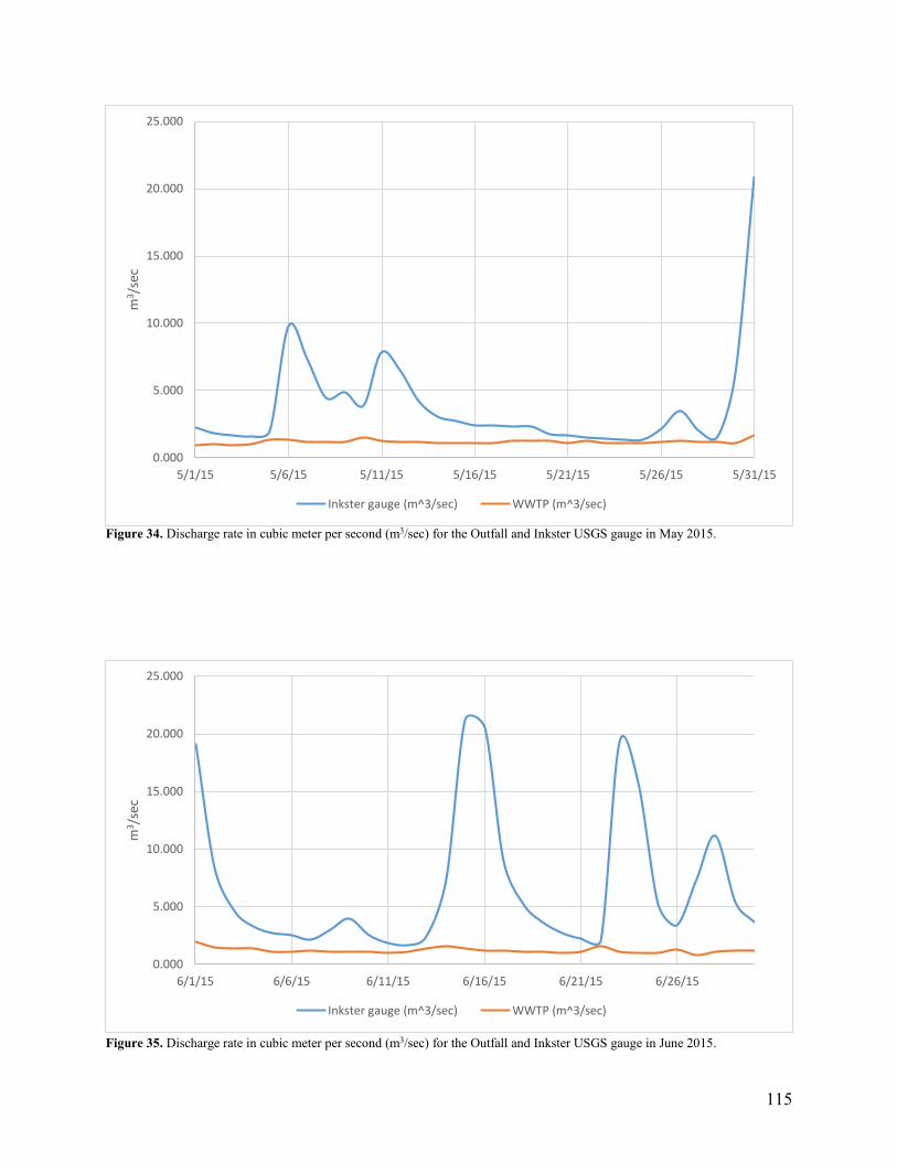
115

Figure 34. Discharge rate in cubic meter per second (m3/sec) for the Outfall and Inkster USGS gauge in May 2015.

Figure 35. Discharge rate in cubic meter per second (m3/sec) for the Outfall and Inkster USGS gauge in June 2015.

0.000

5.000

10.000

15.000

20.000

25.000

5/1/15 5/6/15 5/11/15 5/16/15 5/21/15 5/26/15 5/31/15

m3 /

sec


0.000

5.000

10.000

15.000

20.000

25.000

6/1/15 6/6/15 6/11/15 6/16/15 6/21/15 6/26/15

m3 /

sec


116

Figure 36. Discharge rate in cubic meter per second (m3/sec) for the Outfall and Inkster USGS gauge in July 2015.

Figure 37. Discharge rate in cubic meter per second (m3/sec) for the Outfall and Inkster USGS gauge in August 2015.

0.000

5.000

10.000

15.000

20.000

25.000

7/1/15 7/6/15 7/11/15 7/16/15 7/21/15 7/26/15 7/31/15

m3 /

sec


0.000

5.000

10.000

15.000

20.000

25.000

8/1/15 8/6/15 8/11/15 8/16/15 8/21/15 8/26/15 8/31/15

m3 /

sec


117

Figure 38. Discharge rate in cubic meter per second (m3/sec) for the Outfall and Inkster USGS gauge in September 2015.

Figure 39. Discharge rate in cubic meter per second (m3/sec) for the Outfall and Inkster USGS gauge in October 2015.

0.000

5.000

10.000

15.000

20.000

25.000

9/1/15 9/6/15 9/11/15 9/16/15 9/21/15 9/26/15

m3 /

sec


0.000

5.000

10.000

15.000

20.000

25.000

10/1/15 10/6/15 10/11/15 10/16/15 10/21/15 10/26/15

m3 /

sec


118

APPENDIX 6

Past data of macroinvertebrate families for each location from 2012 to 2015 for spring and fall

Table 32. Past spring benthic macroinvertebrate data for Fowl2 2012 to 2015 from FOTR. R means rare (1-10) and C means common (>10). COMMON NAME ORDER FAMILIES (CLASS) DATE DATE DATE DATE

FOWL2 4/18/2015 4/12/2014 4/27/2013 4/24/2010 Caddisfly larvae Trichoptera Limnephilidae - R - R Caddisfly larvae Trichoptera Uenoidae - - - Stonefly nymphs Plecoptera Nemouridae - - - R Mayfly nymphs Ephemeroptera Heptageniidae (Stenacron) C R R C

Beetle Coleoptera Haliplidae (Peltodytes) R - R R Beetle larvae Coleoptera Dytiscidae - - -

Beetle adults Coleoptera Elmidae - - - Black fly larvae Diptera Simuliidae C - C C

Crayfish Decapoda R - R - Damselfly Zygoptera Coenagrionidae - C - - Damselfly Zygoptera Calopterygidae - - C

Net-spinning caddisfly larvae Trichoptera Hydropsychidae (Cheumatosyche) - - R R Scuds Amphipoda Gammaridae (Gammarus) R R R C

Sowbugs Isopoda R C R R Aquatic worms Annelida Oligochaeta R C R R Midge larvae Diptera Chironomidae C C C C Pouch snails Gastropoda Physidae - - - R True bugs Hemiptera Veliidae (Microvelia) R - - - True bugs Hemiptera Corixidae - - R - True bugs Hemiptera Gerridae - - R

Other true flies Diptera Culicidae - - R - Other true flies Diptera Ceratopogonidae R - - -

FAMILY RICHNESS 10 8 12 16

119

Table 33. Past spring benthic macroinvertebrate data for the Outfall 2014 to 2015 from FOTR. R means rare (1-10) and C means common (>10).

COMMON NAME ORDER FAMILIES (CLASS) DATE DATE LR-2 4/17/2015 4/11/2014

Caddisfly larvae Trichoptera Limnephilidae R - Mayfly nymphs Ephemeroptera Heptageniidae (Stenacron)

R -

Mayfly nymphs Ephemeroptera Leptophlebiidae - Beetle adults Coleoptera Elmidae R -

Black fly larvae Diptera Simuliidae C C Clams - R

Crane fly larvae Diptera Tipulidae R - Crayfish - R

Damselfly nymphs Zygoptera Coenagrionidae C R Damselfly nymphs Zygoptera Calopterygidae R -

Net-spinning caddisfly larvae Trichoptera Hydropsychidae (Cheumatosyche) C C Scuds Amphipoda C R

Sowbugs Isopoda R C Aquatic Worms Annelida Oligochaeta R R

Leeches Annelida Hirudinea R - Midge larvae Diptera Chironomidae C C

FAMILY RICHNESS 14 9

120

Table 34. Past spring benthic macroinvertebrate data for LR-12 2012 to 2015 from FOTR. R means rare (1-10) and C means common (>10).

COMMON NAME ORDER FAMILIES (CLASS) DATE DATE DATE DATE LR-12 4/17/2015 4/11/2014 5/9/2013 4/25/2012

Caddisfly larvae Trichoptera Leptoceridae - - - R Mayfly nymphs Ephemeroptera Baetidae R - R

R Mayfly nymphs Ephemeroptera Heptageniidae (Stenacron) R R -

Beetle adults Coleoptera Elmidae R R R R Black fly larvae Diptera Simuliidae C C C C

Clams Pelecypoda Unionidae - - R

- Clams Pelecypoda Sphaeriidae R C R

Crane fly larvae Diptera Tipulidae R R - - Crayfish Decapoda R R R C

Damselfly nymphs Zygoptera Coenagrionidae - - R C

Damselfly nymphs Zygoptera Calopterygidae - R Dragonfly nymphs Odonata Aeshnidae R - - R

Net-spinning caddisfly larvae Trichoptera Hydropsychidae (Cheumatosyche) C C C C Scuds Amphipoda R - C R

Sowbugs Isopoda R C C - Aquatic worms Annelida Oligochaeta R R R R

Leeches Annelida Hirudinea - R R - Midge larvae Diptera Chironomidae C C C C

Limpets Gastropoda Ancylidae R - - - Pouch snails Gastropoda Physidae - -

R -

Gastropoda Planorbidae - - - True bugs Belostomatidae - R - -


121



Mayfly nymphs Ephemeroptera Heptageniidae (Stenacron) - R R R Mayfly nymphs Ephemeroptera Baetidae R - - -

Beetle adults Coleoptera Elmidae - R - - Beetle larvae Coleoptera Elmidae - - - R Beetle adults Coleoptera Haliplidae R - - -

Clams Pelecypoda Sphaeriidae R - R - Crane fly larvae Diptera Tipulidae R - - -

Crayfish Decapoda R R R R Damselfly nymphs Zygoptera Coenagrionidae R

C R

R Damselfly nymphs Zygoptera Calopterygidae R -

Net-spinning caddisfly larvae Trichoptera Hydropsychidae (Cheumatosyche) C R C R Scuds Amphipoda - - - R

Sowbugs Isopoda R R R R Aquatic worms Annelida Oligochaeta R C C C

Leeches Annelida Hirudinea R - - - Midge larvae Diptera Chironomidae C C C C Pouch snail Gastropoda Physidae R - -

R Limpets Gastropoda Ancylidae R - R

True bugs Hemiptera Gerridae R - - - FAMILY RICHNESS 15 9 9 12

122



Mayfly nymphs Ephemeroptera Heptageniidae (Stenacron) - - R - Beetle adults Coleoptera Haliplidae - - R -

Black fly larvae Diptera Simuliidae C R - C Clams Pelecypoda Sphaeriidae - R - R

Crane fly larvae Diptera Tipulidae R R - R Crayfish Decapoda R C R R

Damselfly nymphs Zygoptera Calopterygidae C C R C Damselfly nymphs Zygoptera Coenagrionidae - Dragonfly nymphs Odonata Aeshnidae R - - R

Net-spinning caddisfly larvae Trichoptera Hydropsychidae (Cheumatosyche) C C C C Scuds Amphipoda R R R R

Sowbugs Isopoda R - R - Aquatic worms Annelida Oligochaeta C R R R

Leeches Annelida Hirudinea R R - - Midge larvae Diptera Chironomidae C C C C

Limpets Gastropoda Ancylidae - - R R FAMILY RICHNESS 11 11 11 12

123

Table 37. Past fall benthic macroinvertebrate data for Fowl2 2012 to 2015 from FOTR. R means rare (1-10) and C means common (>10).

COMMON NAME ORDER FAMILIES/CLASS DATE DATE DATE DATE FOWL2 10/17/2015 10/25/2014 10/19/2013 10/20/2012

Mayfly nymphs Ephemeroptera Heptageniidae (Stenacron) C C R R Beetle adults Coleoptera Elmidae - R - R

Clams Pelecypoda Sphaeriidae - - R R Crayfish Decapoda R C R R

Damselfly nymphs Zygoptera Coenagrionidae - - - R

Damselfly nymphs Zygoptera Calopterygidae - R R Dragonfly nymphs Odonata Aeshnidae R - - -

Net-spinning caddisfly larvae Trichoptera Hydropsychidae - R R - Scuds Amphipoda R C R R

Sowbugs Isopoda C R R C Aquatic worms Annelida Oligochaeta R R - R Midge larvae Diptera Chironomidae C C C C Pouch Snail Hygrophila Physidae (Gastropoda) R - - R True bugs Hemiptera Veliidae - - -

R True bugs Hemiptera Corixidae R - -


124

Table 38. Past fall benthic macroinvertebrate data for LR-2 2012 to 2015 from FOTR. R means rare (1-10) and C means common (>10).

COMMON NAME ORDER FAMILIES/CLASS DATE DATE DATE DATE LR-2 10/13/2015 10/23/2014 10/11/2013 10/112/2012

Mayfly nymphs Ephemeroptera Heptageniidae (Stenacron) - - R - Beetle adults Coleoptera Elmidae R - - R Beetle adults Coleoptera Hydrophilidae - R - -

Black fly larvae Diptera Simuliidae R R - R Crane fly larvae Diptera Tipulidae R R - R

Crayfish Decapoda R R - R Damselfly nymphs Zygoptera Calopterygidae R R

R -

Damselfly nymphs Zygoptera Coenagrionidae - - R Dragonfly nymphs Odonata Aeshnidae - R R -

Net-spinning caddisfly larvae Trichoptera Hydropsychidae (Cheumatosyche) C C - C Scuds Amphipoda C R R R

Sowbugs Isopoda R R R R Aquatic Worms Annelida Oligochaeta R R R -

Leeches Annelida Hirudinea R - R - Midge larvae Diptera Chironomidae C R C C Pouch snails Gastropoda Physidae - - R -

Limpets Gastropoda Ancylidae - R - R True bugs Hemiptera Veliidae - - - R


125



Mayfly nymphs Ephemeroptera Heptageniidae (Stenacron) - - C C Mayfly nymphs Ephemeroptera Baetidae C C Beetle adults Coleoptera Elmidae R R C

R Beetle adults Coleoptera Hydrophilidae - - - Beetle adults Coleoptera Dytiscidae - - - Beetle larvae Coleoptera Elmidae - - - C

Black fly larvae Diptera Simuliidae C C C C Clams Pelecypoda Sphaeriidae - - C R

Crane fly larvae Diptera Tipulidae R R R C Crayfish Decapoda R R R R

Damselfly nymphs Zygoptera Calopterygidae R R R R Dragonfly nymphs Odonata Aeshnidae R - R -

Net-spinning caddisfly larvae Trichoptera Hydropsychidae (Cheumatosyche) C C C C Scuds Amphipoda - R R -

Sowbugs Isopoda - - - R Aquatic worms Annelida Oligochaeta - R R R

Flatworm Turbellaria R - Leeches Annelida Hirudinea R R R -

Midge larvae Diptera Chironomidae R C R C Pouch snails Gastropoda Physidae R R Limpets Gastropoda Ancylidae R - True bugs Hemiptera Nepidae - - - R True bugs Hemiptera Veliidae - - R True bugs Hemiptera Belostomatidae - - - True flies Diptera Ceratopogonidae - - R -

FAMILY RICHNESS 12 12 18

126

Table 40. Past fall benthic macroinvertebrate data for LR-6 2012 to 2015 from FOTR. Fall 2014 was not sampled. R means rare (1-10) and C means common (>10).

COMMON NAME ORDER FAMILIES/CLASS DATE DATE DATE DATE LR-6 10/20/2015 10/11/2013 10/12/2012

Mayfly nymphs Ephemeroptera Baetidae R

C - Mayfly nymphs Ephemeroptera Heptageniidae (Stenacron) - R

Beetle adults Coleoptera Elmidae R - - Crane fly larvae Diptera Tipulidae - R -

Crayfish Decapoda R R C Damselfly nymphs Zygoptera Coenagrionidae - R C Damselfly nymphs Zygoptera Calopterygidae R - -

Net-spinning caddisfly larvae Trichoptera Hydropsychidae (Cheumatosyche) C C C Sowbugs Isopoda R R R

Aquatic worms Annelida Oligochaeta R R R Leeches Annelida Hirudinea - R -

Midge larvae Diptera Chironomidae R R C Limpets Gastropoda Ancylidae R C C

True bugs Hemiptera Veliidae (Microvelia) R - - FAMILY RICHNESS 10 10 8

127



Mayfly nymphs Ephemeroptera Baetidae C

R C C Mayfly nymphs Ephemeroptera Heptageniidae (Stenacron) - - -

Beetle adults Coleoptera Elmidae R - - - Clams Pelecypoda Sphaeriidae R - R R

Crane fly larvae Diptera Tipulidae R - - - Crayfish Decapoda R R R C

Damselfly nymphs Zygoptera Coenagrionidae R - - R Damselfly nymphs Zygoptera Calopterygidae R R R -

Net-spinning caddisfly larvae Trichoptera Hydropsychidae (Cheumatosyche) C R C C Scuds Amphipoda R R - -

Sowbugs Isopoda C R - - Aquatic worms Annelida Oligochaeta R R - R

Leeches Annelida Hirudinea - - - R Midge larvae Diptera Chironomidae R C R C

Limpets Gastropoda Ancylidae - R - R True bugs Hemiptera Belostomatidae (Belastoma) R - - -


128

BIBLIOGRAPHY

Allan, J.D., and M.M. Castillo. 2007a. “Streamwater Chemistry.” In Stream Ecology: Structure and Function of Running Waters, 2nd:57–74. Book, Whole. Dordrecht, Netherlands: Springer.

Allan, J.D., and M.M. Castillo. 2007b. “Trophic Relationships.” In Stream Ecology: Structure and Function of Running Waters, 2nd:163–96. Book, Whole. Dordrecht, Netherlands: Springer.

Alston, D.E., J.M. Lawrence, D.R. Bayne, and F.F. Campbell. 1978. “Effects of Thermal Alteration on Macroinvertebrate Fauna in Three Artificial Channels.” In Energy and Environmental Stress in Aquatic Systems, Selected Papers from a Symposium, Held at Augusta, Georgia, edited by J.H. Thorp and J.W. Gibbons, p 569-579. Springfield, Virginia: U.S. Department of Energy.

Barbour, M.T., J. Gerritsen, B.D. Snyder, and J.B. Stribling. 1999. “Rapid Bioassessment Protocols for Use in Streams and Wadeable Rivers: Periphyton, Benthic Macroinvertebrates and Fish.” EPA 841-B-99-002. Washington, DC: U.S. Environmental Protection Agency.

Bêche, L.A., E.P. Mcelravy, and V.H. Resh. 2006. “Long-Term Seasonal Variation in the Biological Traits of Benthic-Macroinvertebrates in Two Mediterranean-Climate Streams in California, U.S.A.” Freshwater Biology 51 (1): 56–75. doi:10.1111/j.1365-2427.2005.01473.x.

Benda, R.S., and M.A. Proffitt. 1974. “Effects of Thermal Effluents on Fish and Invertebrates.” Springfield, Virginia: Aquinas Coll., Grand Rapids; Savannah River Ecology Lab., Aiken, SC (USA).

Bode, R.W., M.A. Novak, L.E. Abele, D.L. Heitzman, and A.J. Smith. 2002. Quality Assurance Work Plan for Biological Stream Monitoring in New York State. Albany, New York: Stream Biomonitoring Unit, Bureau of Monitoring and Assessment, Division of Water, NYS Department of Environmental Conservation.

Bouchard, R.W. 2004. Guide to Aquatic Invertebrates of the Upper Midwest: Identification Manual for Students, Citizen Monitors, and Aquatic Resource Professionals. Minneapolis, MN: University of Minnesota, Water Resources Research Center.

Cairns, J., A.G. Heath, and B.C. Parker. 1975. “The Effects of Temperature upon the Toxicity of Chemicals to Aquatic Organisms.” Hydrobiologia 47 (1): 135–71. doi:10.1007/BF00036747.

129

Caissie, D. 2006. “The Thermal Regime of Rivers: A Review.” Freshwater Biology 51 (8): 1389–1406. doi:10.1111/j.1365-2427.2006.01597.x.

Coulter, D.P., M.S. Sepúlveda, C.D. Troy, and T.O. Höök. 2014. “Thermal Habitat Quality of Aquatic Organisms near Power Plant Discharges: Potential Exacerbating Effects of Climate Warming.” Fisheries Management and Ecology 21 (3): 196–210.

Coutant, C.C. 1962. “The Effect of a Heated Water Effluent upon the Macroinvertebrate Riffle Fauna of the Delaware River.” In Proceedings of the Pennsylvania Academy of Science, 36:58–71.

Coutant, C.C., and A.J. Brook. 1970. “Biological Aspects of Thermal Pollution I. Entrainment and Discharge Canal Effects∗.” Critical Reviews in Environmental Science and Technology 1 (1–4): 341–81.

Crema, R., and A. M. Bonvicini Pagliai. 1980. “The Structure of Benthic Communities in an Area of Thermal Discharge from a Coastal Power Station.” Marine Pollution Bulletin 11 (8): 221–24. doi:10.1016/0025-326X(80)90410-5.

Dahlberg, M.D., and J.C. Conyers. 1974. “Winter Fauna in a Thermal Discharge with Observations on a Macrobenthos Sampler.” In Thermal Ecology, 414–22. Springfield, Virginia: U.S. Department of Energy.

Dallas, H. 2008. “Water Temperature and Riverine Ecosystem: An Overview of Knowledge and Approaches for Assessing Biotic Responses, with Special Reference to South Africa.” Water SA 34: 393–404.

De Stasio, B.T., T. Golemgeski, and D.M. Livingstone. 2009. “Temperature as a Driving Factor in Aquatic Ecosystems.” In Encyclopedia of Inland Waters, 690–98. Oxford: Academic Press. http://www.sciencedirect.com/science/article/pii/B9780123706263000740.

Durance, I., and S. J. Ormerod. 2007. “Climate Change Effects on Upland Stream Macroinvertebrates over a 25-Year Period.” Global Change Biology 13 (5): 942–57. doi:10.1111/j.1365-2486.2007.01340.x.

Durrett, C.W., and W.D. Pearson. 1975. “Drift of Macroinvertebrates in a Channel Carrying Heated Water from a Power Plant.” Hydrobiologia 46 (1): 33–43. doi:10.1007/BF00038725.

Friberg, N., L. Sandin, M.T. Furse, S.E. Larsen, R.T. Clarke, and P. Haase. 2006. “Comparison of Macroinvertebrate Sampling Methods in Europe.” Hydrobiologia 566 (1): 365–78. doi:10.1007/s10750-006-0083-6.

Gooch, J.W., ed. 2007. “Thermal Discharge.” Encyclopedic Dictionary of Polymers. New York, NY: Springer New York. http://dx.doi.org/10.1007/978-0-387-30160-0_11519.

130

Greenacre, M., and R. Primicerio. 2013. “Measures of Distance between Samples: Non-Euclidean.” In Multivariate Analysis of Ecological Data, 59–74. Bilbao, Spain: Fundación BBVA. http://www.fbbva.es/TLFU/dat/greenacre_maed_ch05.pdf.

Gücker, B., M. Brauns, and M.T. Pusch. 2006. “Effects of Wastewater Treatment Plant Discharge on Ecosystem Structure and Function of Lowland Streams.” Journal of the North American Benthological Society 25 (2): 313–29. doi:10.1899/0887-3593(2006)25[313:EOWTPD]2.0.CO;2.

Heip, C. H. R., P. M. J. Herman, and K. Soetaert. 1998. “Indices of Diversity and Evenness.” Océanis (Paris) 24 (4): 67–87.

Hershey, A.E., G.A. Lamberti, D.T. Chaloner, and R.M. Northington. 2010. “Chapter 17 - Aquatic Insect Ecology.” In Ecology and Classification of North American Freshwater Invertebrates (Third Edition), edited by James H. Thorp and Alan P. Covich, 659–94. San Diego: Academic Press.

Hogg, I. D., D. D. Williams, J. M. Eadie, and S. A. Butt. 1995. “The Consequences of Global Warming for Stream Invertebrates: A Field Simulation.” Journal of Thermal Biology, Effects of Rising Temperature on the Ecology and Physiology of Aquatic Organisms, 20 (1–2): 199–206. doi:10.1016/0306-4565(94)00057-P.

Hogg, I. D., and D.D. Williams. 1996. “Response of Stream Invertebrates to a Global-Warming Thermal Regime: An Ecosystem-Level Manipulation.” Ecology 77 (2): 395–407. doi:10.2307/2265617.

Howell, FG, and JB Gentry. 1974. “Effect of Thermal Effluents from Nuclear Reactors on Species Diversity of Aquatic Insects.” Savannah River Ecology Lab., Aiken, SC; Savannah River Ecology Lab., Aiken, SC (USA).

Huryn, A. D. 2009. “Aquatic Insects – Ecology, Feeding, and Life History.” In Encyclopedia of Inland Waters, edited by Gene E. Likens, 132–43. Oxford: Academic Press. http://www.sciencedirect.com/science/article/pii/B9780123706263001599.

Kannan, K., J. Lee Kober, Y.S. Kang, S. Masunaga, J. Nakanishi, A. Ostaszewski, and J.P. Giesy. 2001. “Polychlorinated Naphthalenes, Biphenyls, Dibenzo‐p‐dioxins, and Dibenzofurans as Well as Polycyclic Aromatic Hydrocarbons and Alkylphenols in Sediment from the Detroit and Rouge Rivers, Michigan, USA.” Environmental Toxicology and Chemistry 20 (9): 1878–89.

Kim, H.Y. 2013. “Statistical Notes for Clinical Researchers: Assessing Normal Distribution (2) Using Skewness and Kurtosis.” Restorative Dentistry & Endodontics 38 (1): 52–54.

Langford, T.E. 1971. “The Distribution, Abundance and Life-Histories of Stoneflies (Plecoptera) and Mayflies (Ephemeroptera) in a British River, Warmed by Cooling-Water from a Power Station.” Hydrobiologia 38 (2): 339–77. doi:10.1007/BF00036844.

131

Langford, T.E. 1972. “Comparative Assessment of Thermal Effects in Some British and North American Rivers.” Central Electricity Generating Board, Nottingham, Eng.

Langford, T.E. 1983. Electricity Generation and the Ecology of Natural Waters. Liverpool, United Kingdom: Liverpool University Press.

Langford, T.E. 1990. Ecological Effects of Thermal Discharges. Springer Science & Business Media.

Langford, T.E., and R.J. Aston. 1972. “The Ecology of Some British Rivers in Relation to Warm Water Discharges from Power Stations.” Proceedings of the Royal Society of London. Series B, Biological Sciences 180 (1061): 407–19.

Lehmkuhl, DM. 1972. “Change in Thermal Regime as a Cause of Reduction of Benthic Fauna Downstream of a Reservoir.” Journal of the Fisheries Research Board of Canada 29 (9): 1329–32.

LeRoy Poff, N, and R.A. Matthews. 1986. “Benthic Macroinvertebrate Community Structural and Functional Group Response to Thermal Enhancement in the Savannah River and a Coastal Plain Tributary.” Archiv Für Hydrobiologie 106 (1): 119–37.

Li, F., N. Chung, M.J. Bae, Y.S. Kwon, T.S. Kwon, and Y.S. Park. 2013. “Temperature Change and Macroinvertebrate Biodiversity: Assessments of Organism Vulnerability and Potential Distributions.” Climatic Change 119 (2): 421–34. doi:10.1007/s10584-013-0720-9.

LOSAG, (Lower One Subwatershed Advisory Group). 2001a. “Chapter 2. Introduction to the Lower One Subwatershed Management Plan.” Wayne County, Michigan: Wayne County, Michigan.

LOSAG, (Lower One Subwatershed Advisory Group). 2001b. “Chapter 3. State of the Lower One Subwatershed.” Wayne County, Michigan: Wayne County, Michigan.

LTSAG, (Lower Two Subwatershed Advisory Group). 2001a. “Chapter 1 Intoduction.” Wayne County, Michigan: Wayne County, Michigan.

LTSAG, (Lower Two Subwatershed Advisory Group). 2001b. “Chapter 2 State of the Subwatershed.” Wayne County, Michigan: Wayne County, Michigan.

Macan, T.T. 1960. A Key to the British Fresh-and Brackish-Water Gastropods: With Notes on Their Ecology. Vol. 13. Freshwater biological association.

Maheu, A., A. St-Hilaire, D. Caissie, and N. El-Jabi. 2016. “Understanding the Thermal Regime of Rivers Influenced by Small and Medium Size Dams in Eastern Canada.” River Research and Applications, January, n/a-n/a. doi:10.1002/rra.3046.

Mann, K.H. 1965. “Heated Effluents and Their Effects on the Invertebrate Fauna of Rivers” 14: 45–53.

132

Massengill, RR. 1976. “Benthic Fauna: 1965-1967 Versus 1968-1972.” The Connecticut River Ecological Study, The Impact of a Nuclear Power Plant, American Fisheries Society Monograph, no. 1.

MCWC, (Michigan Clean Water Corps. 2005. “Stream Macroinvertebrate Datasheet - Order Level.” https://micorps.net/wp-content/uploads/VSMP-Macro-OrderLevel-Datasheet.pdf.

Menne, M.J., I. Durre, B. Korzeniewski, S. McNeal, K. Thomas, X. Yin, S. Anthony, et al. 2012a. “Global Historical Climotology Network - Daily (GHCN-Daily), Version 3. [GHCND:US1MIWY0031].”

Menne, M.J., I. Durre, B. Korzeniewski, S. McNeal, K. Thomas, X. Yin, S. Anthony, et al. 2012b. “Global Historical Climotology Network - Daily (GHCN-Daily), Version 3. [GHCND:US1MIWY0068].”

Menne, M.J., I. Durre, B. Korzeniewski, S. McNeal, K. Thomas, X. Yin, S. Anthony, et al. 2012c. “Global Historical Climotology Network - Daily (GHCN-Daily), Version 3. [GHCND:USC00202015].”

Menne, M.J., I. Durre, R.S. Vose, B.E. Gleason, and T.G. Houston. 2012. “An Overview of the Global Historical Climotology Network - Daily Database.” Journal of Atmospheric and Oceanic Technology 29: 897–910. doi:doi:10.1175/JTECH-D-11-00103.1.

Merritt, R.W., K.W. Cummins, M.B. Berg, R.W. Holzenthal, A.L. Prather, and S. A. Marshall, eds. 2008. Introduction to the Aquatic Insects of North America. 4th ed. Dubuque, Iowa: Kendall Hunt Publishing.

Murray, K.S., D. Cauvet, M. Lybeer, and J.C. Thomas. 1999. “Particle Size and Chemical Control of Heavy Metals in Bed Sediment from the Rouge River, Southeast Michigan.” Environmental Science & Technology 33 (7): 987–92.

Murray, K.S., L.E. Fisher, J. Therrien, B. George, and J. Gillespie. 2001. “Assessment and Use of Indicator Bacteria to Determine Sources of Pollution to an Urban River.” Journal of Great Lakes Research 27 (2): 220–29.

Murray, K.S., D.T. Rogers, and M.M. Kaufman. 2004. “Heavy Metals in an Urban Watershed in Southeastern Michigan.” Journal of Environmental Quality 33 (1): 163–72.

Nedeau, E.J., R.W. Merritt, and M.G. Kaufman. 2003. “The Effect of an Industrial Effluent on an Urban Stream Benthic Community: Water Quality vs. Habitat Quality.” Environmental Pollution 123 (1): 1–13. doi:10.1016/S0269-7491(02)00363-9.

Osborne, L.L., and R.W. Davies. 1987. “The Effects of a Chlorinated Discharge and a Thermal Outfall on the Structure and Composition of the Aquatic Macroinvertebrate Communities in the Sheep River, Alberta, Canada.” Water Research 21 (8): 913–21. doi:10.1016/S0043-1354(87)80008-8.

133

Poole, G., J. Risley, and M. Hicks. 2001. “Spatial and Temporal Patterns of Stream Temperature (Revised).” EPA-910-D-01-003. Washington, DC: U.S. Environmental Protection Agency.

Preece, R.M., and H.A. Jones. 2002. “The Effect of Keepit Dam on the Temperature Regime of the Namoi River, Australia.” River Research and Applications 18 (4): 397–414. doi:10.1002/rra.686.

Price, M. 2014. “2013 Rouge River Ecosystem Monitoring and Assessment Report.” Wayne County, Michigan: Wayne County, Michigan, Rouge River National Wet Weather Demonstration Project.

Schueler, T.R. 1994. “The Importance of Imperviousness.” Watershed Protection Techniques 1 (3): 100–111.

Spänhoff, B., R. Bischof, A. Böhme, S. Lorenz, K. Neumeister, A. Nöthlich, and K. Küsel. 2007. “Assessing the Impact of Effluents from a Modern Wastewater Treatment Plant on Breakdown of Coarse Particulate Organic Matter and Benthic Macroinvertebrates in a Lowland River.” Water, Air and Soil Pollution 180 (1–4): 119–29. doi:http://0-dx.doi.org.wizard.umd.umich.edu/10.1007/s11270-006-9255-2.

Stark, J.D., I.K.G. Boothroyd, J.S. Harding, J.R. Maxted, and M.R. Scarsbrook. 2001. “Protocols for Sampling Macroinvertebrates in Wadeable Streams.” New Zealand Macroinvertebrate Working Report No. 1. New Zealand: Ministry for the Environment.

Tiquia, S.M. 2010. “Metabolic Diversity of the Heterotrophic Microorganisms and Potential Link to Pollution of the Rouge River.” Environmental Pollution 158 (5): 1435–43.

Tiquia, S.M. 2011. “Extracellular Hydrolytic Enzyme Activities of the Heterotrophic Microbial Communities of the Rouge River: An Approach to Evaluate Ecosystem Response to Urbanization.” Microbial Ecology 62 (3): 679–89.

Tiquia, S.M., D. Davis, H. Hadid, S. Kasparian, M. Ismail, S. Ahly, J. Shim, S. Singh, and K.S. Murray. 2007. “Halophilic and Halotolerant Bacteria from River Waters and Shallow Groundwater along the Rouge River of Southeastern Michigan.” Environmental Technology 28 (3): 297–307.

Tixier, G., K.P. Wilson, and D.D. Williams. 2008. “Exploration of the Influence of Global Warming on the Chironomid Community in a Manipulated Shallow Groundwater System.” Hydrobiologia 624 (1): 13–27. doi:10.1007/s10750-008-9663-y.

USEPA, (US Environmental Protection Agency). 1997. “Volunteer Stream Monitoring: A Methods Manual.” Washington, DC: US Environmental Protection Agency, Office of Wetlands, Oceans, and Watersheds.

USGS, (U.S. Geological Survey). 2016. “USGS Current Conditions for USGS 04168000 LOWER RIVER ROUGE AT INKSTER, MI.” http://waterdata.usgs.gov/usa/nwis/uv?site_no=04168000.

134

Vannote, R.L., G.W. Minshall, K.W. Cummins, J.R. Sedell, and C.E. Cushing. 1980. “The River Continuum Concept.” Canadian Journal of Fisheries and Aquatic Sciences 37 (1): 130–37. doi:10.1139/f80-017.

Vannote, R.L., and B.W. Sweeney. 1980. “Geographic Analysis of Thermal Equilibria: A Conceptual Model for Evaluating the Effect of Natural and Modified Thermal Regimes on Aquatic Insect Communities.” The American Naturalist 115 (5): 667–95.

Verones, F., M.M. Hanafiah, S. Pfister, M.A.J. Huijbregts, and A. Koehler. 2010. “Characterization Factors for Thermal Pollution in Freshwater Aquatic Environments.” Environmental Science & Technology 44: 9364–69.

Voshell, J. R. Jr. 2002. A Guide to Common Freshwater Invertebrates of North America. First Edition. Blacksburg, Va: McDonald and Woodward Publishing Company.

Wallace, J.B., and N.H. Anderson. 1996. “Habitat, Life History, and Behavioral Adaptations of Aquatic Insects.” In Introduction to the Aquatic Insects of North America, edited by Richard W. Merritt and Kenneth W. Cummins, 3th:41–73. Book, Whole. Dubuque, Iowa: Kendall Hunt Publishing.

Wallace, J.B., and J.R. Webster. 1996. “The Role of Macroinvertebrates in Stream Ecosystem Function.” Annual Review of Entomology 41 (1): 115–39. doi:10.1146/annurev.en.41.010196.000555.

Wellborn, G.A., and J.V. Robinson. 1996. “Effects of a Thermal Effluent on Macroinvertebrates in a Central Texas Reservoir.” American Midland Naturalist 136 (1): 110–20. doi:10.2307/2426636.

Wiley, M.J., P.W. Seelbach, and S.P. Bowler. 1998. “Ecological Targets for Rehabilitation of the Rouge River.” Ann Arbor, Michigan: School of Natural Resources and Environment.

Worthington, T. A., P. J. Shaw, J. R. Daffern, and T. E. L. Langford. 2015. “The Effects of a Thermal Discharge on the Macroinvertebrate Community of a Large British River: Implications for Climate Change.” Hydrobiologia 753 (1): 81–95. doi:10.1007/s10750-015-2197-1.

Wurtz, C.B., and W.F. Skinner. 1984. “A Twelve-Year Macroinvertebrate Study in the Vicinity of Two Thermal Discharges to the Susquehanna River Near York Haven, PA.” Journal of Testing and Evaluation 12 (3): 157–62. doi:10.1520/JTE11068J.

YCUA, (Ypsilanti Community Utilities Authority). 2012a. “Antidegradation Demonstration for Increasing Loading.” Courtesy paper from YCUA.

YCUA, (Ypsilanti Community Utilities Authority). 2012b. “State Revolving Fund Project Plan.” Ypsilanti, Michigan: YCUA. http://ycua.org/PDFs/2012SRFProjectPlanReport.pdf.

YCUA, (Ypsilanti Community Utilities Authority). 2014. “YCUA’s Wastewater Treatment Process.” http://ycua.org/PDFs/WWTPBrochure.pdf.

135

YCUA, (Ypsilanti Community Utilities Authority). 2016. “Ypsilanti Community Utilities Authority: About Us.” Accessed July 15. http://ycua.org/about.htm.

the effect of wastewater treatment plant effluent on water

Documents