WORKING PAPER SERIES

The Effectiveness of Monetary Policy: An Assessment

Yi Wen

Working Paper 2005-052A

http://research.stlouisfed.org/wp/2005/2005-052.pdf

June 2005

FEDERAL RESERVE BANK OF ST. LOUIS Research Division 411 Locust Street

St. Louis, MO 63102 ______________________________________________________________________________________

The views expressed are those of the individual authors and do not necessarily reflect official positions of the Federal Reserve Bank of St. Louis, the Federal Reserve System, or the Board of Governors.

Federal Reserve Bank of St. Louis Working Papers are preliminary materials circulated to stimulate discussion and critical comment. References in publications to Federal Reserve Bank of St. Louis Working Papers (other than an acknowledgment that the writer has had access to unpublished material) should be cleared with the author or authors.

Photo courtesy of The Gateway Arch, St. Louis, MO. www.gatewayarch.com

The E¤ectiveness of Monetary Policy:An Assessment�

Yi WenDepartment of Economics

Cornell UniversityIthaca, NY 14853

(This version: 2000)

Abstract

When monetary policies are endogenous, the conventional VAR approach for detecting thee¤ect of monetary policies is powerless. This paper proposes to test the implication of monetarypolicies along a di¤erent dimension. That implication is to exploit the policy induced exogeneityof endogenous variables that are the source of monetary non-neutrality. We illustrate the ideaby constructing a new Keynesian sticky wage model with capital accumulation and then testingthe implications of optimal monetary policies for nominal wages under both complete andincomplete information. Econometric test using post war US data suggests that the nominalwage is exogenous with respect to lagged macro variables. Such exogeneity is consistent withnew Keynesian models in which the monetary authority pursues active monetary policy basedon information with a lag.

Keywords: Optimal monetary policy; Sticky wages; Sticky prices; Business Cycles.

JEL Classi�cation : E52, E41, E32.

�I would like to thank Eric Leeper, Peter Pedroni, and seminar participants at Indiana University Bloomingtonfor valuable comments. Correspondence: Yi Wen, Department of Economics, Cornell University, Ithaca, NY 14853.Tel. 607-255-6339. Email yw57@cornell.edu.

1

1 Introduction

For decades, detecting the non-neutrality of money using VARs has been the major means

to find out the real effects of monetary policy. The power of VARs for detecting the effects of

money, however, relies largely on the identifying assumption that monetary policy changes be

exogenous, so as to render meaningful the notion of “monetary policy shocks” in an impulse

responses analysis. Unfortunately, it is hard to deny that the so called “monetary policy shocks”

are often endogenous. The endogeneity of monetary policy implies that VAR’s can fail to identify

the mechanisms through which monetary policy affects the real economy as well as the true

magnitude of that effect, because money can fail to appear as a significant dependent variable in

a VAR when it is endogenous.1

To illustrate, denote st as the vector of the state variables that all agents in the economy

observe in period t, denote ct as the vector of decision variables of the private sector, and assume

that monetary policy follows the linear feedback rule mt = αst.2 Suppose a rational-expectations

general-equilibrium model has the reduced-form first-order conditions given by:

Et

⎡⎣ st+1

ct+1

⎤⎦ = A

⎡⎣ st

ct

⎤⎦+B1Etmt+1 +B2mt,

in which the monetary policy, m, is taken as parametric by the private sector of the economy.

According to classical theory, B1 = B2 = 0, hence money does not influence the real economy.

According to Keynesian theory, B1, B2 6= 0 and money does have real consequences.

The fact that the matrices B 6= 0, however, does not at all imply that the effects of money can

be detected by VARs. To see that, substitute out the monetary policy rule by αs in the equation,

we get:

Et

⎡⎣ st+1

ct+1

⎤⎦ = (I − αB1)−1 (A+ αB2)

⎡⎣ st

ct

⎤⎦ .1In a comprehensive econometric analysis, Leeper, Sims, and Zha (1996) showed that most VAR specifications

imply that only a modest (or in some cases, essentially none) of the variance of output or prices in the US since

1960 is attributable to shifts in monetary policy, and on the other hand, that a large fraction of the variation in

monetary policy instruments is attributable to systematic reaction by policy authors to the state of the economy.

They conclude that “This is of course what we would expect of good monetary policy, but it is also the reason

why using the historical behavior of aggregate time series to uncover the effects of monetary policy is difficult.”2If α is time-dependent and is itself a function of the state, we can linearize the monetary feedback rule,

mt = α(st)st, around a steady state to get a similar formula.

2

Solving for the system forward under tranversality conditions and rational expectations, the

equilibrium decision rules obtained by the private sector then take the form:

ct = c (α, st) ,

which reflects the Lucas Critique that the forward looking private sector’s decision rules are not

invariant to the monetary policy α. It follows that the state variables in the economy evolve

according to the equilibrium law of motion:

st+1 = s (α, st) .

The control vector c can also be expressed in a VAR form:

ct+1 = c (α, ct) ,

where the mapping c may be singular.

It is then clear that in a correctly specified VAR model for the economy, money fails to show

up as a significant dependent variable when it is endogenous. That is, money fails to Granger

cause endogenous variables such as st+1 in a VAR even if it does have real influences on st+1.

In such a case, it is difficult not only to measure the effectiveness of monetary policy, but

also to distinguish the classical theory from the Keynesian theory by VARs. In the classical case,

money fails to show up in a VAR as a significant dependent variable because B1 = B2 = 0. In the

Keynesian case, money also fails to show up as a significant dependent variable in a VAR simply

due to the endogenouty of monetary policy. If the monetary authority should follow a passive

money growth rule according to monetarism, VARs will also be incapable of fully identifying the

real effects of money.

This paper proposes to assess the effectiveness of monetary policy by testing the implication of

endogenous monetary policy along a different dimension. That implication is the policy-induced

exogeneity of some endogenous variables that are the source of monetary non-neutrality.

According to the new Keynesian theory, short-run price or nominal wage stickiness are the

culprit of monetary non-neutrality. If this is the case, then optimal monetary policies aiming at

stabilizing the economy will render some of the price variables completely “sticky”, so that they

become completely independent of any endogenous variables in the economy.3

3On the other hand, if prices adjust instantaneously as in the neoclassical theory, then they ought to be

determined by endogenous variables that influence supply and demand. Hence, they ought to be themselves

endogenous.

3

To illustrate, suppose there are two nominal prices in an economy, p1 and p2, and that p1

is temporarily sticky in the sense that it is influenced by two forces at any point of time: one

pertaining to its own history, reflecting price inertia or stickiness, and the other pertaining to

market clearing forces, indicating that supply and demand will rule in the long run. These

assumptions suggest that the log of p1t can be characterized by:

log p1t =kX

j=1

θj log p1t−j + (1− θ) log p∗1t,kX

j=1

θj = θ ∈ [0, 1], k ≤ ∞; (1)

where p∗1 is the equilibrium market-clearing price that adjust instantaneously to demand and

supply. That is, p∗1 satisfies:

log p∗1 = log p2 + f(x),

where x denotes equilibrium quantities in the economy.

In the neoclassical economy, the relative price, (log p∗1 − log p2), is completely determined by

the market forces f(x) and is independent of the influence of money.4 In the new Keynesian

economy, the relative price, (log p1 − log p2), is not completely determined by market forces, and

money is not neutral in the short run:

log p1t − log p2 =kX

j=1

θj log p1t−j + (1− θ) log p∗1t − log p2 (2)

=kX

j=1

θj log p1t−j + (1− θ)f(x)− θ log p2.

The goal of an optimal monetary policy is then to choose money supply such that the relative

price in the Keynesian economy behaves in the same way as it does in a classical economy:

log p1 − log p2 = f(x).

To achieve that, equation 2 suggests that the monetary authority should set the level of money

supply such that

log p2 =1

θ

kXj=1

θj log p1t−j − f(x).

This implies

log p1t =1

θ

kXj=1

θj log p1t−j.

4Since f(·) is homogeneous of degree zero in money, it can be viewed as independent of money.

4

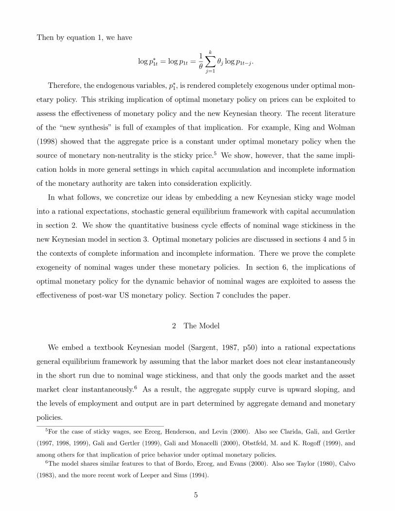
Then by equation 1, we have

log p∗1t = log p1t =1

θ

kXj=1

θj log p1t−j.

Therefore, the endogenous variables, p∗1, is rendered completely exogenous under optimal mon-

etary policy. This striking implication of optimal monetary policy on prices can be exploited to

assess the effectiveness of monetary policy and the new Keynesian theory. The recent literature

of the “new synthesis” is full of examples of that implication. For example, King and Wolman

(1998) showed that the aggregate price is a constant under optimal monetary policy when the

source of monetary non-neutrality is the sticky price.5 We show, however, that the same impli-

cation holds in more general settings in which capital accumulation and incomplete information

of the monetary authority are taken into consideration explicitly.

In what follows, we concretize our ideas by embedding a new Keynesian sticky wage model

into a rational expectations, stochastic general equilibrium framework with capital accumulation

in section 2. We show the quantitative business cycle effects of nominal wage stickiness in the

new Keynesian model in section 3. Optimal monetary policies are discussed in sections 4 and 5 in

the contexts of complete information and incomplete information. There we prove the complete

exogeneity of nominal wages under these monetary policies. In section 6, the implications of

optimal monetary policy for the dynamic behavior of nominal wages are exploited to assess the

effectiveness of post-war US monetary policy. Section 7 concludes the paper.

2 The Model

We embed a textbook Keynesian model (Sargent, 1987, p50) into a rational expectations

general equilibrium framework by assuming that the labor market does not clear instantaneously

in the short run due to nominal wage stickiness, and that only the goods market and the asset

market clear instantaneously.6 As a result, the aggregate supply curve is upward sloping, and

the levels of employment and output are in part determined by aggregate demand and monetary

policies.

5For the case of sticky wages, see Erceg, Henderson, and Levin (2000). Also see Clarida, Gali, and Gertler

(1997, 1998, 1999), Gali and Gertler (1999), Gali and Monacelli (2000), Obstfeld, M. and K. Rogoff (1999), and

among others for that implication of price behavior under optimal monetary policies.6The model shares similar features to that of Bordo, Erceg, and Evans (2000). Also see Taylor (1980), Calvo

(1983), and the more recent work of Leeper and Sims (1994).

5

Specifically, a representative household chooses sequences of consumption {ct}∞t=0 , real money

balancenmt

pt

o∞t=0

, capital stock {kt+1}∞t=0 , and labor supply {nst}∞t=0 , taking as given the real

wagesnwtpt

o∞t=0

and real rental rates {rt}∞t=0 to solve

maxE0

∞Xt=0

βt

(log (ct) + φ log

µmt

pt

¶− a

(nst)1+γ

1 + γ

)subject to:

ct +mt

pt+ kt+1 − (1− δ)kt =

wt

ptnt + rtkt +

mt−1xtpt

,

where the gross growth rate of money supply, xt = mt/mt−1, is also taken as exogenous by the

private sector.

Assuming that the goods market clears instantaneously, the first-order necessary conditions

for optimality are then given by:

a (nst)γ =

1

ct

wt

pt(3)

φ³mt

pt

´ = 1

ct− βEt

1

ct+1

ptpt+1

xt+1 (4)

1

ct= βEt

1

ct+1(rt+1 + 1− δ) (5)

ct + kt+1 − (1− δ)kt =wt

ptnt + rtkt (6)

mt = mt−1xt (7)

where (3) relates optimal labor supply to the real wage, (4) gives the optimal demand for real

money balance, (5) characterizes the optimal consumption demand, (6) relates aggregate demand

for goods to aggregate real income (the goods market clearing condition), and (7) equates nominal

money demand to supply. Notice that equation (4) can be written as:

φ =mt

ptct− βEt

mt+1

pt+1ct+1,

which can be solved forward under a transversality condition to get:

mt

ptct=

φ

1− β,

which reflects the quantity theory of money and where the right-hand side can be interpreted as

the inverse velocity of money.

A representative firm produces output y according to a constant returns to scale production

technology:

yt = Atkαt n

1−αt ,

6

where At represents random shocks to productivity. In each period, the firm chooses the demand

for labor ndt and capital kt, taking the real wage and rental rate as given to solve

max

½Atk

αt n

1−αt − wt

ptnt − rtkt

¾.

The firm’s optimal demand for labor and capital inputs are then given by the first-order conditions:

(1− α)Atkt¡ndt¢−α

=wt

pt

αAtkα−1t

¡ndt¢1−α

= rt,

which also implies the zero profit condition:

wt

ptndt + rtkt = Atk

αt

¡ndt¢1−α

.

The optimal demand for labor is then given by:

ndt = (1− α)1α A

1αt kt

µptwt

¶ 1α

.

Substituting this labor demand schedule into the production function gives the aggregate supply

function:

yt = (1− α)1−αα A

1αt kt

µptwt

¶ 1−αα

,

which is upward sloping with regard to the price level pt.

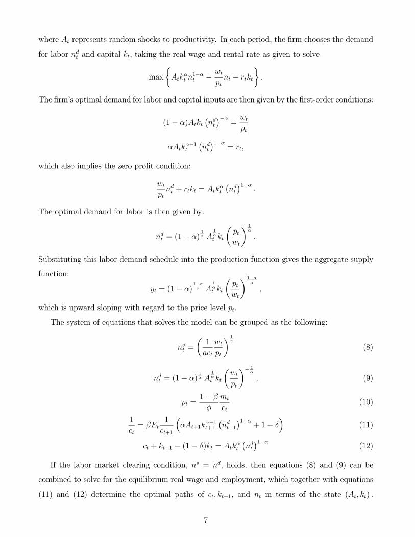
The system of equations that solves the model can be grouped as the following:

nst =

µ1

act

wt

pt

¶ 1γ

(8)

ndt = (1− α)1α A

1αt kt

µwt

pt

¶− 1α

, (9)

pt =1− β

φ

mt

ct(10)

1

ct= βEt

1

ct+1

³αAt+1k

α−1t+1

¡ndt+1

¢1−α+ 1− δ

´(11)

ct + kt+1 − (1− δ)kt = Atkαt

¡ndt¢1−α

(12)

If the labor market clearing condition, ns = nd, holds, then equations (8) and (9) can be

combined to solve for the equilibrium real wage and employment, which together with equations

(11) and (12) determine the optimal paths of ct, kt+1, and nt in terms of the state (At, kt) .

7

Equation (10) then determines the price level. This is the classical result in which money is a

veil.7

Due to stickiness in the nominal wage wt, however, the household’s labor supply ns does not

always equal to the firm’s labor demand, nd. Hence we cannot use the labor market clearing

condition to solve for employment. Instead, the level of employment (the effective labor demand

nd) has to be determined by equilibrium in the goods market. That is, the system of equations for

solving the model becomes (after substituting out the effective labor demand nd using equation

9):

pt =1− β

φ

mt

ct(13)

1

ct= βEt

1

ct+1

Ãα (1− α)

1−αα A

1αt+1

µwt+1

pt+1

¶− 1−αα

+ 1− δ

!(14)

ct + kt+1 − (1− δ)kt = (1− α)1−αα A

1αt kt

µwt

pt

¶− 1−αα

(15)

Notice that money matters in such an economy because it affects the price level p, which in terns

affects the aggregate demand and aggregate supply through its effect on the real wage w/p.

In a standard Keynesian model, in place of the labor market clearing condition is an equation

that specifies exogenously the short-run behavior of the nominal wage. We assume that the

nominal wage is influenced by two forces: one pertains to the history of nominal wages, reflecting

wage inertia or stickiness due to institutional factors or staggered wage setting behavior; and

the other pertains to market forces from demand and supply. We assume that in the long run

nominal wages are determined solely by demand and supply of labor. Under these assumptions,

the log of nominal wage can be characterized by:

logwt =kX

j=0

θj logwt−j + (1− θ) logw∗t , (16)

wherePk

j=1 θj = θ ∈ [0, 1], k ≤ ∞, and where w∗ is the equilibrium nominal wage determined by

the market clearing condition:

ns = nd.

Hence, w∗ is given by (using equation 8 and the condition ns = nd):

w∗t = a¡ndt¢γ

ptct.

7In the classical model, the equilibrium nominal wage is a function of the state: wt = f(kt, At). It is therefore

not exogenous with respect to current macro conditions. In the case that the technology shocks are serially

correlated, the nominal wage is also in part predictable by lagged variables such as lagged output.

8

Equation system (13) - (16) represents the textbook version of the Keynesian model in a

dynamic, rational expectations setting. The Keynesian model has a simple form of analytical

solution when the rate of capital depreciation δ = 1. In such a case, the decision rule for kt+1 is

given by:

kt+1 = βαyt = βα

"(1− α)

1−αα A

1αt kt

µwt

pt

¶− 1−αα

#.

If we define the net aggregate supply as yt − kt+1, then the net supply function is given by:

log(yt − kt+1)

=

½log(1− βα) (1− α)

1−αα +

1

αlogAt + log kt −

1− α

αlogwt

¾+1− α

αlog pt.

According to equation 13, the net aggregate demand function is given by:

log ct = log1− β

φ+ logmt − log pt.

Using a standard price-quantity diagram, the above supply curve is upward sloping and the

demand curve is downward sloping (see figure 1).

Figure 1. The “Keynesian” effect of a decrease in nominal wage.

Due to the stickiness in the nominal wage, a decrease in the money supply shifts the demand

curve inward, causing a reduction in the equilibrium quantities of net output and consumption.

On the other hand, a decrease in the nominal wage raises the aggregate supply, which shifts the

supply curve upward, resulting in a drop in the equilibrium price level and an increase in the

equilibrium quantities. This “Keynesian effect”of changes in the nominal wage on equilibrium

quantity and price is shown in figure 1. It is also clear from the diagram that the central bank

9

should conduct an expansionary monetary policy to shift the demand curve upward when facing

an adverse supply shock (such as an oil price increase) which shifts the supply curve downward.

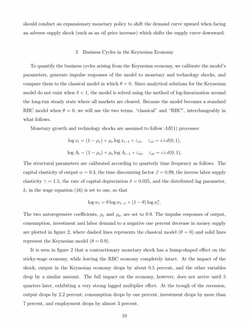
3 Business Cycles in the Keynesian Economy

To quantify the business cycles arising from the Keynesian economy, we calibrate the model’s

parameters, generate impulse responses of the model to monetary and technology shocks, and

compare them to the classical model in which θ = 0. Since analytical solutions for the Keynesian

model do not exist when δ < 1, the model is solved using the method of log-linearization around

the long-run steady state where all markets are cleared. Because the model becomes a standard

RBC model when θ = 0, we will use the two terms, “classical” and “RBC”, interchangeably in

what follows.

Monetary growth and technology shocks are assumed to follow AR(1) processes:

log xt = (1− ρx) + ρx log xt−1 + εxt, εxt ∼ i.i.d(0, 1),

logAt = (1− ρa) + ρa logAt−1 + εat, εat ∼ i.i.d(0, 1),

The structural parameters are calibrated according to quarterly time frequency as follows. The

capital elasticity of output α = 0.3, the time discounting factor β = 0.99, the inverse labor supply

elasticity γ = 1.5, the rate of capital depreciation δ = 0.025, and the distributed lag parameter,

k, in the wage equation (16) is set to one, so that

logwt = θ logwt−1 + (1− θ) logw∗t .

The two autoregressive coefficients, ρx and ρa, are set to 0.9. The impulse responses of output,

consumption, investment and labor demand to a negative one percent decrease in money supply

are plotted in figure 2, where dashed lines represents the classical model (θ = 0) and solid lines

represent the Keynesian model (θ = 0.9).

It is seen in figure 2 that a contractionary monetary shock has a hump-shaped effect on the

sticky-wage economy, while leaving the RBC economy completely intact. At the impact of the

shock, output in the Keynesian economy drops by about 0.5 percent, and the other variables

drop by a similar amount. The full impact on the economy, however, does not arrive until 5

quarters later, exhibiting a very strong lagged multiplier effect. At the trough of the recession,

output drops by 2.2 percent, consumption drops by one percent, investment drops by more than

7 percent, and employment drops by almost 3 percent.

10

The recovery from the business cycle trough is very slow. It takes about 60 quarters for output

to reach its pre-shock level from the business cycle trough. Such persistent effects of monetary

shocks on an sticky-wage economy is very typical and they will be discussed further below in

comparison with the case of technology shocks.

The impulse responses to a negative one percent decrease in technology are shown in figure 3,

where the dashed lines represent the RBC model and solid lines represent the Keynesian model.

Sticky nominal wages render the economy more volatile than the RBC economy in response to

technology shocks. For example, output in the sticky wage model drops by 2 percent at the impact

of the technology shock, as oppose to 1.3 percent in the flexible wage model. Table 1 summarizes

some selected second moments of the two economies. It shows that the variance of output in

the sticky wage model is about (?) times that in the RBC model. Higher volatilities induced

by the nominal wage stickiness reduce welfare because they hinder consumption smoothing and

intertemporal substitutions.

The reason why output is more volatile in the presence of sticky nominal wages is obvious.

Due to a decrease in productivity, the marginal product of labor also decreases. Since nominal

wage is sticky, which results in stickiness in the marginal cost of labor, the marginal benefit of

labor must be kept from decreasing in order to maximize profit. This compels firms to cut labor

demand more than necessary in order to maintain the desired level of the marginal product of

labor. Hence output falls more than necessary. Consequently, both consumption and investment

also fall more than they do in the RBC model.

Another feature of the impulse responses to technology shocks in the sticky wage model is

the fast recovery relative to the classical model after a technology shock. It takes output only

4 quarters and employment only 2 quarters respectively to recover half of their pre-shock levels,

as oppose to 9 quarters and 6 quarters respectively in the flexible wage model. Such a speed of

recovery is especially striking when being compared to the case under a monetary shock (figure

2), where the length of half-life recovery is at least 4-5 times longer starting from the business

cycle trough.

A. Inspecting the Propagation Mechanism

Why do recoveries take so much longer under monetary shocks than under technology shocks?

The answer lies in the different propagation mechanisms of the sticky wage economy with regard to

the two different sources of shocks. Under technology shocks, the main mechanism for propagating

11

the impact of the shock is through capital accumulation. The speed of labor market adjustment

plays little role in magnifying that propagation. On the other hand, under monetary shocks, the

main propagation mechanism is the sluggish labor market adjustment.

To see the differences in the propagation mechanisms, consider a simpler version of the sticky

wage model where the rate of capital depreciation δ = 1 and where the inverse elasticity of labor

supply γ = 0. The log-linearized equilibrium output is given by the production function in (15):

yt =1

αAt + kt +

1− α

α(pt − wt) .

Since kt = βαyt−1 and pt =1−βφ

mt

ct, we have

yt =1

αAt + yt−1 +

1− α

α(mt − ct − wt) .

Substituting out consumption by the decision rule: ct = (1 − βα)yt, the above equation (after

re-arrangement) can be further reduced to:

yt = αyt−1 + At + (1− α)mt − (1− α)wt.

The nominal wage can be expressed as distributed lags in money supply:

wt = θwt−1 + (1− θ)w∗t

= θwt−1 + (1− θ) (γnt + pt + ct)

= θwt−1 + (1− θ)mt

=1− θ

1− θLmt,

where L is the lag operator. Hence the nominal wage is constant without monetary shocks.

Namely, wt = mt = 0. This implies that the law of motion for the output in the absence of

monetary shocks follows:

yt = αyt−1 +At.

It is clear then that the impact of technology shocks is propagated in output over time purely

through the technology parameter α, which also governs the speed of capital accumulation in the

model.

On the other hand, under monetary shocks, the law of motion for output follows:

yt = αyt−1 + (1− α)mt − (1− α)1− θ

1− θLmt,

12

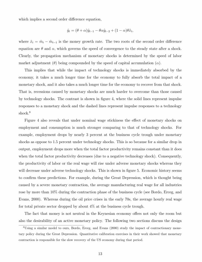
which implies a second order difference equation,

yt = (θ + α)yt−1 − θαyt−2 + (1− α)θxt,

where xt = mt − mt−1 is the money growth rate. The two roots of the second order difference

equation are θ and α, which governs the speed of convergence to the steady state after a shock.

Clearly, the propagation mechanism of monetary shocks is determined by the speed of labor

market adjustment (θ) being compounded by the speed of capital accumulation (α).

This implies that while the impact of technology shocks is immediately absorbed by the

economy, it takes a much longer time for the economy to fully absorb the total impact of a

monetary shock, and it also takes a much longer time for the economy to recover from that shock.

That is, recessions caused by monetary shocks are much harder to overcome than those caused

by technology shocks. The contrast is shown in figure 4, where the solid lines represent impulse

responses to a monetary shock and the dashed lines represent impulse responses to a technology

shock.8

Figure 4 also reveals that under nominal wage stickiness the effect of monetary shocks on

employment and consumption is much stronger comparing to that of technology shocks. For

example, employment drops by nearly 3 percent at the business cycle trough under monetary

shocks as oppose to 1.5 percent under technology shocks. This is so because for a similar drop in

output, employment drops more when the total factor productivity remains constant than it does

when the total factor productivity decreases (due to a negative technology shock). Consequently,

the productivity of labor or the real wage will rise under adverse monetary shocks whereas they

will decrease under adverse technology shocks. This is shown in figure 5. Economic history seems

to confirm these predictions. For example, during the Great Depression, which is thought being

caused by a severe monetary contraction, the average manufacturing real wage for all industries

rose by more than 10% during the contraction phase of the business cycle (see Bordo, Erceg, and

Evans, 2000). Whereas during the oil price crises in the early 70s, the average hourly real wage

for total private sector dropped by about 4% at the business cycle trough.

The fact that money is not neutral in the Keynesian economy offers not only the room but

also the desirability of an active monetary policy. The following two sections discuss the design

8Using a similar model to ours, Bordo, Erceg, and Evans (2000) study the impact of contractionary mone-

tary policy during the Great Depression. Quantitative calibration exercises in their work showed that monetary

contraction is responsible for the slow recovery of the US economy during that period.

13

and the implementation of optimal monetary policies that eliminate the inefficiency caused by

sticky nominal wages, as well as the econometric implications for testing the effectiveness of these

policies.

4 Optimal Monetary Policy under Complete Information

A first-best outcome is defined as the resource allocation in the RBC model (θ = 0) in which

the labor market clears instantaneously. As is seen earlier, output is less volatile in the RBC

model in response to exogenous shocks. In comparison, a larger volatility of output arises in the

Keynesian model due to the fact that the real wage fails to equate labor supply and labor demand

because of nominal wage rigidity. Precisely due to that rigidity, however, monetary policy has

real influence on the real wage.

Proposition 1 In order to replicate the RBC allocation, an optimal monetary policy should seek

to achieve:

w∗t = w (wt−1, wt−2,, ..., wt−k) ,

where

log w (wt−1, wt−2,, ..., wt−k) ≡1

θ

kXj=1

θj logwt−j.

Proof. To replicate the neoclassical allocation, an optimal monetary policy should seek to

replicate the real wage that clears the labor market. Since the real wage in the sticky wage model

follows (use equation 16):

wt

pt=

wθ1t−1...w

θkt−k

pθt

µw∗tpt

¶1−θ,

in order to have wtpt= w∗t

pt,we must have w∗t =

hwθ1t−1...w

θkt−k

i 1θ,or

logw∗t =1

θ

kXj=0

θjwt−j.

¥

Remark 1 By equation (16), the above also implies:

logwt = logw∗t =

1

θ

kXj=1

θj logwt−j.

14

Hence, the real wage in the Keynesian model under the recommended policy becomes:

w (wt−1, wt−2,, ..., wt−k)

pt= anγt ct. (4.1)

Substituting the real wage into the labor demand function (9) immediately yields the same condi-

tion that would obtain in the classical model where the labor market clears instantaneously.

Proposition 2 To implement the optimal monetary policy, the monetary authority should set

the money supply according to:

mt =φ

1− β

w (wt−1, wt−2,, ..., wt−k)

anγt. (4.2)

Proof. Combining equations 13 and 17 gives:

w = anγt ptct = anγt1− β

φmt,

which implies

mt =φ

1− β

w

anγt.

¥

Remark 2 Proposition 2 suggests that it is always possible to implement optimal monetary policy

according to (18) such that the market clearing wage, w∗t , behaves just like the sticky part of the

nominal wage:

w∗t = anγt1− β

φmt

= w (wt−1, wt−2,, ..., wt−k) .

Consequently, the real wage is ensured to follow

w (wt−1, wt−2,, ..., wt−k)

pt= anγt ct,

and the nominal wage is ensured to follow9

wt = w∗t = w (wt−1, wt−2,, ..., wt−k) . (4.3)

9Notice that the policy works regardless of the value of θ (i.e., even in the case θ = 1 where nominal wage is

perfectly sticky). This is so because for any type of nominal wage rigidity, we need only to choose money supply

according to (18) so that the real wage is ensured to follow (17).

15

Corollary 3 When the labor supply is infinitely elastic, the optimal monetary policy is to follow

a passive rule by setting money growth rate to the wage inflation rate.

Proof. When the labor supply is infinitely elastic, we have γ = 0. Equation (18) implies that

money supply follows a passive rule.¥One of the most striking implications of optimal monetary policies in the new Keynesian model

is the policy-induced complete exogeneity of nominal wage behavior given by equation (19). That

implication can be exploited to test the effectiveness of the US monetary policy.

A. Decision Making under Endogenous Monetary Policy

To obtain a deeper understanding on the influence of monetary policy when agents are forward

looking, it is instructive to see how the private sector actually derive optimal decision rules under

rational expectations in the presence of endogenous monetary policy.

Log linearize the first order conditions (13)-(15) around the long-run steady state under the

specified sticky wage process (16), we can arrive at the following reduced-form system of linear

equations:

Et

⎡⎢⎢⎢⎢⎢⎢⎢⎢⎢⎢⎢⎢⎣

ct+1

kt+1

At+1

wt

...

wt−k+1

⎤⎥⎥⎥⎥⎥⎥⎥⎥⎥⎥⎥⎥⎦=M

⎡⎢⎢⎢⎢⎢⎢⎢⎢⎢⎢⎢⎢⎣

ct

kt

At

wt−1...

wt−k

⎤⎥⎥⎥⎥⎥⎥⎥⎥⎥⎥⎥⎥⎦+R1Etmt+1 +R2mt

⎡⎣ ndt

pt

⎤⎦ = Z1

⎡⎢⎢⎢⎢⎢⎢⎢⎢⎢⎢⎢⎢⎣

kt

ct

At

wt−1...

wt−k

⎤⎥⎥⎥⎥⎥⎥⎥⎥⎥⎥⎥⎥⎦+ Z2mt,

where a hat variable xt denotes percentage deviations from its steady state value x: xt ≡ log xt−

log x. The state variables include the initial capital stock, the level of technology, the history

of nominal wages, and the monetary policy: {kt, At, wt−1, ...wt−k,mt} . The control variable is

consumption ct. Solving for the above system forward under transversality conditions, the linear

16

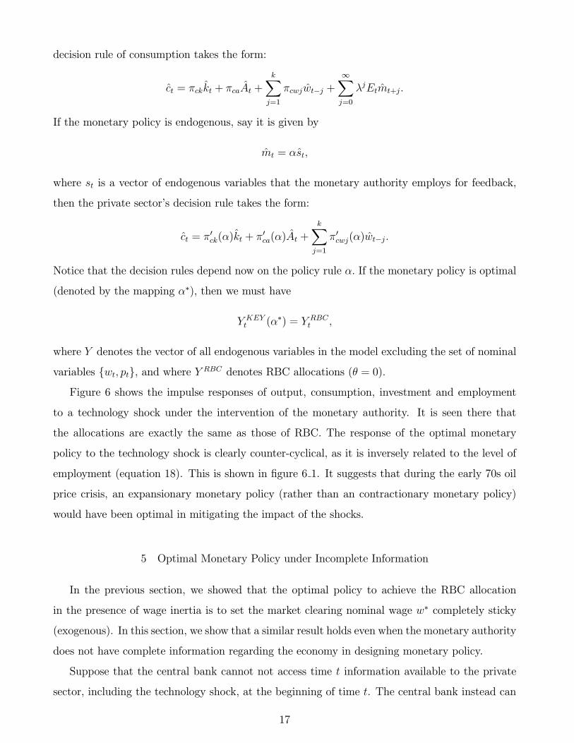
decision rule of consumption takes the form:

ct = πckkt + πcaAt +kX

j=1

πcwjwt−j +∞Xj=0

λjEtmt+j.

If the monetary policy is endogenous, say it is given by

mt = αst,

where st is a vector of endogenous variables that the monetary authority employs for feedback,

then the private sector’s decision rule takes the form:

ct = π0ck(α)kt + π0ca(α)At +kX

j=1

π0cwj(α)wt−j.

Notice that the decision rules depend now on the policy rule α. If the monetary policy is optimal

(denoted by the mapping α∗), then we must have

Y KEYt (α∗) = Y RBC

t ,

where Y denotes the vector of all endogenous variables in the model excluding the set of nominal

variables {wt, pt}, and where Y RBC denotes RBC allocations (θ = 0).

Figure 6 shows the impulse responses of output, consumption, investment and employment

to a technology shock under the intervention of the monetary authority. It is seen there that

the allocations are exactly the same as those of RBC. The response of the optimal monetary

policy to the technology shock is clearly counter-cyclical, as it is inversely related to the level of

employment (equation 18). This is shown in figure 6 1. It suggests that during the early 70s oil

price crisis, an expansionary monetary policy (rather than an contractionary monetary policy)

would have been optimal in mitigating the impact of the shocks.

5 Optimal Monetary Policy under Incomplete Information

In the previous section, we showed that the optimal policy to achieve the RBC allocation

in the presence of wage inertia is to set the market clearing nominal wage w∗ completely sticky

(exogenous). In this section, we show that a similar result holds even when the monetary authority

does not have complete information regarding the economy in designing monetary policy.

Suppose that the central bank cannot not access time t information available to the private

sector, including the technology shock, at the beginning of time t. The central bank instead can

17

only observe the state of the economy with one period lag. What is the optimal monetary policy

in that circumstance? To facilitate discussions, we use log-linearized version of the model in the

following discussions.

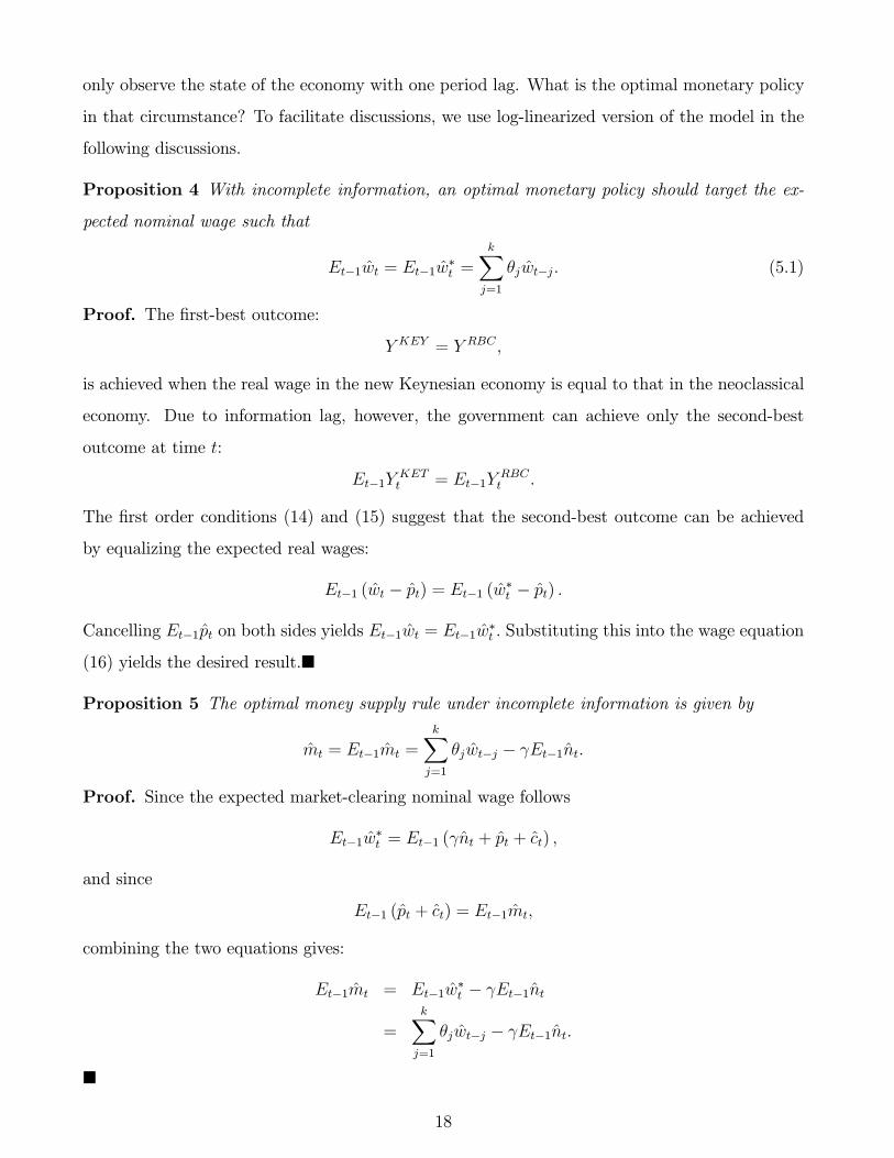
Proposition 4 With incomplete information, an optimal monetary policy should target the ex-

pected nominal wage such that

Et−1wt = Et−1w∗t =

kXj=1

θjwt−j. (5.1)

Proof. The first-best outcome:

Y KEY = Y RBC ,

is achieved when the real wage in the new Keynesian economy is equal to that in the neoclassical

economy. Due to information lag, however, the government can achieve only the second-best

outcome at time t:

Et−1YKETt = Et−1Y

RBCt .

The first order conditions (14) and (15) suggest that the second-best outcome can be achieved

by equalizing the expected real wages:

Et−1 (wt − pt) = Et−1 (w∗t − pt) .

Cancelling Et−1pt on both sides yields Et−1wt = Et−1w∗t . Substituting this into the wage equation

(16) yields the desired result.¥

Proposition 5 The optimal money supply rule under incomplete information is given by

mt = Et−1mt =kX

j=1

θjwt−j − γEt−1nt.

Proof. Since the expected market-clearing nominal wage follows

Et−1w∗t = Et−1 (γnt + pt + ct) ,

and since

Et−1 (pt + ct) = Et−1mt,

combining the two equations gives:

Et−1mt = Et−1w∗t − γEt−1nt

=kX

j=1

θjwt−j − γEt−1nt.

¥

18

Corollary 6 Under the optimal monetary policy that achieves (20), the nominal wage is com-

pletely exogenous in the sense that no lagged variables except its own history has predictive power

on the nominal wage w∗t .

Proof. Equation (20) implies the linear projection:

w∗t =kX

j=1

θjwt−j + et,

where the error term, et ≡ w∗t − Et−1w∗t , satisfies Et−1et = 0, implying that it is orthogonal to

time t− 1 information set.¥It is instructive to demonstrate how et is related to time t innovations in technology, as the

demonstration also illustrates how agents solve for the decision rules under endogenous monetary

policy with incomplete information.

Notice that the reduced-form first order conditions in the Keynesian economy can be charac-

terized by:

Et

⎡⎢⎢⎢⎢⎢⎢⎢⎢⎢⎢⎢⎢⎣

kt+1

ct+1

At+1

wt

...

wt−k+1

⎤⎥⎥⎥⎥⎥⎥⎥⎥⎥⎥⎥⎥⎦=M

⎡⎢⎢⎢⎢⎢⎢⎢⎢⎢⎢⎢⎢⎣

kt

ct

At

wt−1...

wt−k

⎤⎥⎥⎥⎥⎥⎥⎥⎥⎥⎥⎥⎥⎦+R1Etmt+1 +R2mt. (5.2)

Taking expectation on both sides of the equation against t− 1 information set, and substituting

out the monetary policy by mt = αEt−1st gives:

Et−1

⎡⎢⎢⎢⎢⎢⎢⎢⎢⎢⎢⎢⎢⎣

kt+1

ct+1

At+1

wt

...

wt−k+1

⎤⎥⎥⎥⎥⎥⎥⎥⎥⎥⎥⎥⎥⎦= (I −R1α)

−1 (M +R2α)Et−1

⎡⎢⎢⎢⎢⎢⎢⎢⎢⎢⎢⎢⎢⎣

kt

ct

At

wt−1...

wt−k

⎤⎥⎥⎥⎥⎥⎥⎥⎥⎥⎥⎥⎥⎦,

where the monetary policy rule α remains to be determined, and st ≡hkt ct At wt−1 · · · wt−k

i0.10

Solving for the system forward under transversality conditions gives a decision rule for expected

10It can be shown easily that any endogenous monetary rule can be reduced to a form depending on the vector

s.

19

consumption:

Et−1ct = πcsEt−1s1t, (5.3)

where the new state vector s1t ≡hkt At wt−1 · · · wt−k

i0. Given the specified AR(1) tech-

nology shock process, the expected state vector s1t can be written as

s2t = Et−1s1t =hkt ρaAt−1 wt−1 · · · wt−k

i0,

which is known in time period t − 1. Hence, the optimal monetary policy under incomplete

information is given by (after substituting out the expected consumption):

mt = α0s2t, (5.4)

which is the same as Et−1mt since s2t is known in time period t− 1.

Substituting the monetary policy rule (23) into the original system (24), we can solve for the

decision rule of consumption:

ct = π0csSt,

where the state vector St includes lagged technology At−1 :

St =hkt At At−1 wt−1 · · · wt−k

i0.

As a result, all variables y in the economy are determined by St :

yt = πysSt,

including the nominal wage w∗t :

w∗t = wt = πwsSt.

Hence, the one-step ahead forecasting error, et, follows

wt −Et−1wt

= πws (St −Et−1St)

= πwsh0 εat 0 0 0 0

i0= πws[2]εat.

This shows how et depends on the innovations in technology shocks. Consequently, the nominal

wage w∗t (wt−1, ..., wt−k, et) is completely exogenous in the sense that no lagged variables except

its own history has predictive power on its current behavior.

20

The quantitative effectiveness of optimal monetary policy under incomplete information are

shown in figure 7. It is seen there that due to the information lag, the central bank is not able

to mitigate the technology shock at the impact period, hence it is impossible to fully achieve

the RBC allocation. The central bank’s intervention, nevertheless, substantially improves the

economy’s performance in the subsequent periods. For example, the Okun’s gap in terms of

output is substantially reduced compared to the case of no intervention (see figure 8). The

variance of output is reduced by ? percent under the policy intervention.

6 An Econometric Assessment

The fact that the nominal wage is rendered completely exogenous under optimal monetary poli-

cies has the implication for testing the effectiveness of monetary policy in a Keynesian economy.

In the case of complete information, the nominal wage is independent of both contemporaneous

and lagged endogenous variables. In the case of incomplete information, the nominal wage may

be correlated with contemporaneous variables because innovations in technology also affect other

endogenous variables, but it is independent of the history of any endogenous variables. Hence we

develop two types of test for the effectiveness of the post-war US monetary policy, both of which

are kin to the Granger causality test.

The first type tests whether the nominal wage (wt) is correlated with any contemporaneous

endogenous variables, given its own history (wt−j, j = 1, 2, ...). The lack of such correlation

indicates both monetary non-neutrality and the effectiveness of monetary policy.

The second type tests whether the nominal wage is correlated with any lagged endogenous

variables given its own history. The lack of Granger causality from lagged endogenous variables

supports the view of monetary non-neutrality and the effectiveness of monetary policy.11

A. Granger Test 1: Complete Information

We estimate the following equations for the US economy (1964:1-1995:2):

wt = f(wt−j), j = 1, 2, ...k; (A)

11If the actual economy is a classical one, then the nominal wage is predictable by lagged endogenous variables

such as output, as long as technology shocks or any fundamental shocks are serially correlated. Even if these

shocks are not serially correlated, habit formation in labor supply (Wen, 1998) and dynamic labor adjustment

costs (Sargent, 1987, p199) all render the nominal wage dependent on lagged endogenous variables.

21

wt = f (wt−j,Xt) , j = 1, 2, ...k; (B)

wt = f (wt−j , xt) , j = 1, 2, ...k; (C)

wt = f (wt−j, pt) , j = 1, 2, ...k; (C)

where all variables are in growth rates, and where w denotes the nominal wage, x is a vector of

real variables that influence the labor supply and labor demand decisions, including the aggregate

consumption, the rate of capacity utilization (we use GDP as the proxy), the level of employment,

and the money stock, m. X is simply the nominal counterpart of x, and p is the price index (GDP

deflator). We choose the number of lags k = 10 in each regression.

We use two aggregate wage series in our test. One is the average hourly earnings for production

workers in the manufacturing sector, and another is the average hourly earnings for the total

private sector. The OLS estimation results are reported in table 1 and table 2, where values in

the third to fifth column indicate the significance level of a corresponding set of variables under

the F test. Estimating (1) to (4) using manufacturing wage series gives the following results:

Table 1. Manufacturing Sector

Equation R2 F − Test (Xt) F − Test (xt) F − Test (pt) D −W stat.

(A) 0.68 1.99

(B) 0.77 0.08 2.21

(C) 0.77 0.22 1.93

(D) 0.74 0.000002 1.98

Table 1 shows that the manufacturing nominal wage is exogenous with respect to Xt and xt

(at the 5% significance level), but not with respect to pt. The current price inflation rate has

a very significant predicting power on the current wage inflation rate. However, with regard to

the wage series for the total private sector, all the contemporaneous variables, Xt, xt, and pt,

that influence labor supply and demand, do have significant predictive power on the behavior of

nominal wage, as can be seen from table 2 below:

Table 2. Total Private Sector

Equation R2 F − Test (Xt) F − Test (xt) F − Test (pt) D −W stat.

(A) 0.73 2.00

(B) 0.81 0.003 2.47

(C) 0.77 0.0015 1.91

(D) 0.78 0.000009 1.89

22

It is worth mentioning that money growth rate is always an insignificant variable in predicting

the behavior of the nominal wage, indicating the endogeneity of the money supply. According to

our theoretical models, if money were exogenous, the wage inflation rate is at least in part related

to money growth rate by the equation:

wt = f (γnt +mt) .

Hence, money should have predictive power on the nominal wage unless it is endogenous.

The overall results indicate that if the central bank has complete information and has been

pursuing active monetary policy, then the monetary policy has not been very effective in fine-

tuning the economy.

B. Granger Test 2: Incomplete Information

The results in the above section could imply, however, that the central bank is not able to

act immediately to respond to economic shocks due to incomplete information (information lag).

This subsection tests the effectiveness of monetary policy under that circumstance. According

to our earlier analyses, with incomplete information, an active monetary policy will result in

nominal wages that are not predictable by lagged endogenous variables. Both table 3 and table

4 indicate that this is broadly true for the US economy. Namely, the nominal wages are broadly

exogenous with respect to lagged variables. The only exception is that the lagged price inflation

rate appears to be significant at the 5% level in predicting the manufacturing nominal wage. The

inflation rate has no predictive power on the total private sector’s nominal wage. No variables in

Xt−1 or xt−1 have predictive power on either wage series.

Table 3. Manufacturing Sector

Equation R2 F − Test (Xt−1) F − Test (xt−1) F − Test (pt−1) D −W stat.

(A) 0.68 1.99

(B) 0.78 0.62 2.09

(C) 0.68 0.88 1.98

(D) 0.69 0.04 1.98

23

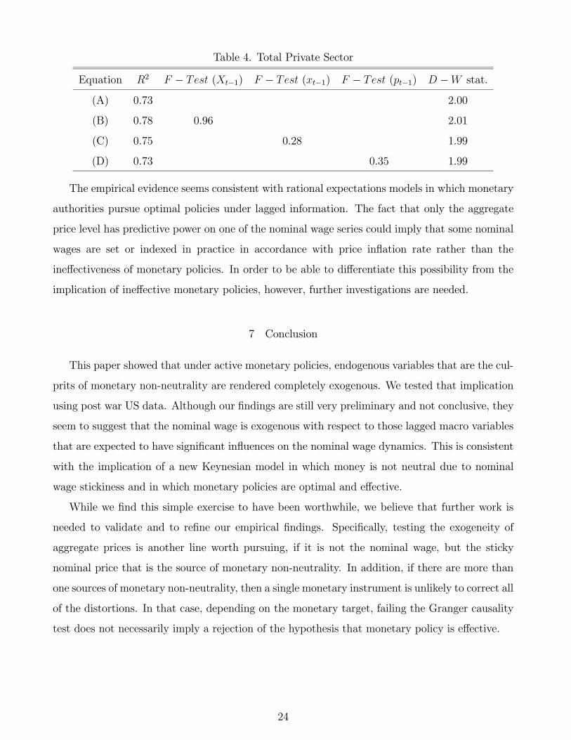
Table 4. Total Private Sector

Equation R2 F − Test (Xt−1) F − Test (xt−1) F − Test (pt−1) D −W stat.

(A) 0.73 2.00

(B) 0.78 0.96 2.01

(C) 0.75 0.28 1.99

(D) 0.73 0.35 1.99

The empirical evidence seems consistent with rational expectations models in which monetary

authorities pursue optimal policies under lagged information. The fact that only the aggregate

price level has predictive power on one of the nominal wage series could imply that some nominal

wages are set or indexed in practice in accordance with price inflation rate rather than the

ineffectiveness of monetary policies. In order to be able to differentiate this possibility from the

implication of ineffective monetary policies, however, further investigations are needed.

7 Conclusion

This paper showed that under active monetary policies, endogenous variables that are the cul-

prits of monetary non-neutrality are rendered completely exogenous. We tested that implication

using post war US data. Although our findings are still very preliminary and not conclusive, they

seem to suggest that the nominal wage is exogenous with respect to those lagged macro variables

that are expected to have significant influences on the nominal wage dynamics. This is consistent

with the implication of a new Keynesian model in which money is not neutral due to nominal

wage stickiness and in which monetary policies are optimal and effective.

While we find this simple exercise to have been worthwhile, we believe that further work is

needed to validate and to refine our empirical findings. Specifically, testing the exogeneity of

aggregate prices is another line worth pursuing, if it is not the nominal wage, but the sticky

nominal price that is the source of monetary non-neutrality. In addition, if there are more than

one sources of monetary non-neutrality, then a single monetary instrument is unlikely to correct all

of the distortions. In that case, depending on the monetary target, failing the Granger causality

test does not necessarily imply a rejection of the hypothesis that monetary policy is effective.

24

References

1. Bordo, M., C. Erceg, and C. Evans, 1997, Money, sticky wages, and the Great Depression,NBER Working Paper No. W6071.

2. Calvo, G., 1983, Staggered prices in a utility-maximizing framework, Journal of MonetaryEconomics 12, 383-398.

3. Clarida, R., J. Gali, and M. Gertler, 1997, Monetary policy rules and macroeconomic stability:Evidence and some theory, Quarterly Journal of Economics, forthcoming.

4. Clarida, R., J. Gali, and M. Gertler, 1998, Monetary policy rules in practice: some interna-tional evidence, European Economic Review 42, 1033-1067.

5. Clarida, R., J. Gali, and M. Gertler, 1999, The science of monetary policy: A new Keynesianperspective, Journal of Economic Literature, forthcoming.

6. Erceg C., D. Henderson, and A. Levin, 2000, Optimal monetary policy with staggered wageand price contracts, Journal of Monetary Economics 46, 281-313.

7. Gali, J. and M. Gertler, 1999, Inflation dynamics: Astructural econometric analysis, Journalof Monetary Economics 44, 195-222.

8. Gali, J. and T. Monacelli, 2000, Optimal monetary policy and exchange rate volatility in asmall open economy, University of Pompeu Fabra.

9. King, R. and A. Wolman, 1998, What should the monetary authority do when prices aresticky? NBER Volume on Monetary Policy Rules, edited by J. Taylor.

10. Leeper, E. and C. Sims, 1994, Toward a modern macroeconomic model usable for policyanalysis, NBER Working Paper Series no. 4761.

11. Leeper, E., C. Sims and T. Zha, 1996, What Does Monetary Policy Do? Presented at theBrookings Panel on Economic Activity, September 8, 1996

12. Obstfeld, M. and K. Rogoff, 1999, New directions for stochastic open economy models, NBERWorking Paper W7313.

13. Sargent, T., 1987, Macroeconomic Theory, Second Edition, Academic Press, London.

14. Taylor, J., Aggregate dynamics and staggered contracts, Journal of Political Economy 88,1-24.

25

Figure 2. Impulse Responses to a Negative Money Supply Shock

26

Figure 3. Impulse Responses to a Negative Technology Shock

27

Figure 4. Comparison of Different Impact of Technology and MonetaryShocks.

28

Figure 5. 29

Figure 6. The Effectiveness of Monetary Policy under Full Information.

30

Figure 7. The Effectiveness of Monetary Policy under IncompleteInformation.

31

Figure 8. Okun's Gap with and without Policy Intervention.

32