the effects of financial crises on international trade · zihui ma is lecturer of international...

This PDF is a selection from a published volume from theNational Bureau of Economic Research

Volume Title: International Trade in East Asia, NBER-EastAsia Seminar on Economics, Volume 14

Volume Author/Editor: Takatoshi Ito and Andrew K. Rose,editors

Volume Publisher: University of Chicago Press

Volume ISBN: 0-226-37896-9

Volume URL: http://www.nber.org/books/ito_05-1

Conference Date: September 5-7, 2003

Publication Date: August 2005

Title: The Effects of Financial Crises on International Trade

Author: Zihui Ma, Leonard Cheng

URL: http://www.nber.org/chapters/c0196

253

8.1 Introduction

The world suffered three major financial crises in the last ten years,namely, the European Monetary System (EMS) crisis in 1992–1993, theMexican crisis in 1994–1995 (which spread to a number of South Ameri-can countries), and the Asian crisis in 1997–1998. Economists usually be-lieve these crises were the results of weak economic fundamentals, for ex-amples, declining foreign reserve, increasing foreign debt, capital accountand current account deficits, fiscal deficit, and so on.

Obviously, a current account deficit can be a very important factor be-cause, other things being equal, it increases foreign debt, decreases foreignreserves, and weakens confidence in the exchange rate of the domesticcurrency. Almost all countries that suffered financial crises had faced ris-ing current account deficits before the crises occurred. So such deficits arewidely regarded as an important factor of financial crises.

International trade links play an important role in the so-called conta-gious effect, that is, a crisis in one country causes a new crisis in anothercountry with relatively good fundamentals. Glick and Rose (1999) pro-vided some analysis of the relationship between trade and contagion, while

Zihui Ma is lecturer of international economics at Renmin University of China. Leon-ard K. Cheng is professor and department head of economics at the Hong Kong Universityof Science and Technology.

We thank Chin Hee Hahn, Kozo Kiyota, Andrew Rose and other seminar participants atthe Fourteenth NBER-East Asia Seminar on Economics for helpful comments and sugges-tions. The work described in this paper was substantially supported by a grant from the Re-search Grant Council of the Hong Kong Special Administrative Region, China (Project no.HKUST6212/00H).

8The Effects of Financial Crises on International Trade

Zihui Ma and Leonard K. Cheng

Forbes (2001) went further to construct some statistics measuring the im-portance of trade linkages in transmitting crises.

Because most economists agree that international trade is one of the im-portant factors in explaining financial crises, it seems natural and logicalto ask the reverse question: what are the effects of financial crises on inter-national trade? Surprisingly, little research on this subject has been done.Perhaps the reason is that the answer appears to be obvious. Conventionalwisdom would predict that a financial crisis, by bringing about a recessionin the macroeconomy, would lead to a drop in imports. Exports, however,may rise because of both a decline in domestic demand and a devaluationof the domestic currency. A weakening or collapse of the financial system,in particular the banking system, however, might weaken the country’s ex-port capability. So the aggregate effects of a financial crisis on the macro-economy are unclear. This paper tries to ascertain whether the ambiguitycan be resolved empirically.

We divide all the past financial crises into two types: banking crises andcurrency crises. These two different types of crises had different attributesand different effects on international trade. This paper begins by analyzingtheoretically the effects of banking and currency crises on internationaltrade. Then it uses bilateral trade data, macroeconomic data, and geo-graphic data to test the theoretical predictions. Overall, the empirical re-sults provide support for the theoretical predictions.

This paper contributes to the literature in two ways. First, it provides atheoretical framework for understanding the impact of financial crises oninternational trade and the channels of crises transmission through trade.Second, it estimates the effects of banking crises and currency crises on im-ports and exports. The estimated results can be used to predict the impactof financial crises on trade, thus providing useful information for risk man-agement to policymakers.

The remainder of the paper is organized as follows. Section 8.2 reviewsprevious works on the relationship between international trade and finan-cial crisis. Sections 8.3 and 8.4 analyze the effects of banking crises and ofcurrency crises on trade, respectively. Section 8.5 describes the data andmethods used to estimate the effects of these crises. Section 8.6 reports theresults of empirical estimation and statistical testing. Section 8.7 con-cludes.

8.2 Literature Review: Trade and Financial Crises

Economists pay attention to the role played by trade in financial crisesfor two reasons. First, trade imbalance has been shown to be one of the im-portant factors that trigger financial crises. Current deficits may decreaseforeign reserves. As Krugman (1979) pointed out, a currency crisis is morelikely to happen in an economy that does not have enough foreign reserves.

254 Zihui Ma and Leonard K. Cheng

Second, financial crises may be transmitted through trade linkages from anaffected country to others despite the latter’s relatively good fundamentals.In explaining such contagion effects, economists have tried to identify thechannels through which contagion was spread. As trade is the most obvi-ous economic linkage between countries, much research has been devotedto this connection. While the importance of trade imbalance in triggeringcrises is widely accepted, there is no agreement on the importance of tradein transmitting financial crises.

Eichengreen and Rose (1999) used a binary-probit model to test whetherbilateral trade linkages transmitted crises between industrial countries be-tween 1959 and 1993. They found that the probability of a financial crisisoccurring in a country increased significantly if the country had high bi-lateral trade linkages with countries in crises. They concluded that tradewas an important factor. Glick and Rose (1999) conducted a similar anal-ysis with more countries between 1971 and 1997 and obtained a similar re-sult. Forbes (2000) used a company’s stock market data to study the impor-tance of trade in financial crises transmission, and his result also showedthat trade played an important role.

However, other papers have provided different answers to the problem.For instance, Baig and Goldfajn (1998) thought that trade linkage was un-important in the East Asian Crisis because the direct bilateral trade vol-umes between these economies were very small. Masson (1998), analyzingthe Mexican crisis and the Asian crisis, obtained similar results.

All the papers that analyzed the relationship between trade and financialcrises ignored the reverse question: how did financial crises affect interna-tional trade? We argue that the effects of financial crises on trade are a pre-condition for discussing whether trade transmits crises. If financial crisesdo not affect countries’ imports and exports at all, how can financial crisesbe transmitted through the trade channel? So before we analyze the im-portance of trade in transmitting financial crises, we need to clarify theeffects of financial crises on international trade. As pointed out previously,little work has been done on this topic to date. It seems there is a belief thatfinancial crises only affect countries’ imports and exports through changesin the exchange rates. Because the effects of exchange rates have alreadybeen thoroughly analyzed before, it may seem that there is no need to studythe question. However, this view may not be correct.

A devaluation of a national currency will increase the volume of exportsand reduce the volume of imports. Classic international trade theory showsthat a devaluation improves the trade balance if the Marshall-Lerner con-dition is satisfied. Because in a financial crisis a country usually experi-enced a devaluation of its national currency, the same analysis would ap-ply, that is, the affected countries’ imports will decrease, but their exportswill increase after the crises.

Furthermore, financial crises (including currency crises, banking crises,

The Effects of Financial Crises on International Trade 255

or both) could also affect trade through channels besides the exchange rate.Calvo and Reinhart (1999) pointed out that financial crises usually causedcapital account reversal (sudden stop) and triggered an economic reces-sion. Mendoza (2001) showed that in an economy with imperfect creditmarkets these sudden stops could be an equilibrium outcome. The eco-nomic recession reduces not only domestic demand but also total outputand export capability, whereas capital outflow forces the country to in-crease export. Thus, whether exports increase or decrease after financialcrises is unclear without further analysis.

Before we analyze how financial crises affect the crisis countries’ importsand exports, let us first define financial crises. Eichengreen and Bordo(2002) have provided definitions of currency crises and banking crises:

For an episode to qualify as a currency crisis, we must observe a forcedchange in parity, abandonment of a pegged exchange rate, or an inter-national rescue. For an episode to qualify as a banking crisis, we mustobserve either bank runs, widespread bank failures and suspension ofconvertibility of deposits into currency such that the latter circulates ata premium relative to deposits (a banking panic), or significant bankingsector problems (including but not limited to bank failures) resulting inthe erosion of most or all of banking system collateral that are resolvedby a fiscally-underwritten bank restructuring. (15–16)

The above definitions are adopted in this paper. In the next two sections,we analyze the effects of banking crises and currency crises on the macro-economy and trade.

8.3 Impact of Banking Crises

A classical framework of bank runs was developed by Diamond and Dy-bvig (1983). Let us recapitulate the key elements of their model. Agents areendowed with goods that can be invested in a long-term project or storedwithout costs. The long-term project is profitable but illiquid, that is, if in-vestors do not liquidate the project before it matures, its return is greaterthan the initial investment; however, if the project is liquidated before itmatures, the fire-sale return is less than the initial investment. Each agentcan be impatient or patient with fixed probabilities, but there is no aggre-gate uncertainty, that is, the total number of impatient agents is fixed andknown by all agents. At the beginning, agents do not know their own typesbut must decide if they will invest in the project. After they have invested(or have decided not to invest), but before the project matures, each agentrealizes his or her own type. Impatient agents must consume immediately,whereas patient agents do not consume anything until the project matures.Agents’ types are private information, so even if each agent knows his orher own type, other people do not know.


On the one hand, if an agent does not invest in the project but turns outto be patient, then the agent has missed a profitable investment opportu-nity. On the other hand, if the agent invests in the project but turns out tobe impatient, the agent will have suffered a loss. In this case, the agent hasto liquidate the long-term investment before it matures.

Agents can improve their utilities by pooling risk through the creation ofa bank. All agents deposit their goods in the bank. Depending on the num-ber of impatient agents, the bank sets aside a part of deposits as reservesand invests the rest in the project. When agents realize their types, impa-tient agents withdraw their deposits from the bank’s reserves and patientagents wait for the project to mature. After the project matures, the bankdistributes the return of the project to patient agents. By way of poolingrisk through the bank, impatient agents do not suffer fire-sale losses, andpatient agents can enjoy the benefits of the project.

However, there is a problem because agents’ types are private informa-tion. Patient agents can pretend to be impatient and withdraw their de-posits before the project matures. Normally, they have no incentive to doso because withdrawing early decreases their utilities. However, patientagents may wish to withdraw their deposits if there is panic. When that hap-pens, the bank’s reserves will not be enough to meet the agents’ demand.The bank has to liquidate the long-term project before it matures, but itcannot meet the withdrawal if all patient agents try to withdraw becausethe fire-sale return of the project is less than the initial investment. Theresult is a bank run, and some agents get nothing back.

The preceding is the classical framework of bank runs. It does not ana-lyze the effect of bank runs on imports and exports. We extend this modelto feature international trade by making four additional assumptions.

1. We assume that agents belong to two categories: local agents and for-eign agents. Local agents are endowed with local goods, and foreign agentsare endowed with foreign goods. Both foreign and local agents may be pa-tient or impatient with the same probability. Both local and foreign goodscan be bought and sold in the international market.

2. The long-term project needs both foreign and local goods as inputs,and it produces local goods. As the aggregate investment increases, the in-vestment demand for local and foreign goods also increases. For simplic-ity, we assume that foreign agents’ deposits are less than the investment de-mand for the foreign goods. So the bank always has to export some localgoods for the sake of importing foreign goods.

3. Foreign agents only consume foreign goods, and local agents con-sume both local and foreign goods. The returns that agents receive from thebank are local goods, so they need to exchange a part or all of the returnfor foreign goods in the international market.

4. There are overlapping generations. When the project matures, a new


generation of agents appears. Like the previous generation, they deposittheir goods in the bank, and the bank invests deposits in a new long-termproject. We assume that the number of local agents is fixed, but the num-ber of foreign agents depends on the experience of the previous generation.If no bank run occurs in the previous generation, the number of new for-eign agents will be the same. Otherwise, the number of new foreign agentswill decrease, that is, capital inflow decreases after a bank run.

We can analyze the impact of banking crises on imports and exports un-der the preceding assumptions. If a bank run occurs before the project ma-tures, all agents withdraw their deposits. Due to the illiquidity of the proj-ect, only some of them can get their deposits back. On the average, agentssuffer losses. All foreign agents (without a bank run, only impatient foreignagents) leave the economy bringing with them the withdrawal. After thebanking crisis, capital inflow decreases. So banking crises affect interna-tional trade through three channels.

1. Income channel. If a bank run occurs, the bank has to liquidate thelong-term investment before it matures, and all depositors suffer somelosses. With a lower income, local agents’ demand for foreign goods goesdown. Through this channel, both imports and exports decrease duringand after banking crises.

2. Foreign capital flow channel. In the absence of bank runs, patient for-eign agents withdraw after the project matures, but the withdrawal wouldbe offset by an inflow of new investment made by the next generation of for-eign agents. However, a bank run causes them to withdraw early and alsoreduces new foreign investment in the future. So banking crises can stimu-late exports during crises but reduce them after crises.

3. Investment demand channel. As aggregate investment decreases, theinput demand for foreign goods drops. So banking crises have negativelonger-term effects on imports through this channel. On the other hand, asforeign investment decreases, the economy must export more local goodsto import foreign goods as investment input. As a result, banking criseswill simulate exports after crises.

The real world is more complicated than that highlighted in the preced-ing theoretical framework. For instance, developed countries usually maybe able to defend their banking systems when banking crises occurred, sonet capital outflow might not happen. As a second example, some less-developed countries (e.g., some African countries) are unsuccessful inattracting a lot of foreign capital, so the impact of capital flow would be in-significant during banking crises. As a third example, several Latin Ameri-can countries (e.g., Mexico, Brazil, and Venezuela) stopped repaying for-eign debt during debt crises in the 1980s, so the amount of net foreign


capital outflow would be less than that suggested by the theoretical anal-ysis.

8.4 Impact of Currency Crises

Currency crises often occur due to one of two reasons: runaway fiscaldeficits or external shocks. We analyze them in turn. As Krugman (1979)pointed out, if a government cannot control its budget deficit, it has to fi-nance the deficit by printing money, thus triggering currency depreciation.The currency crises in Brazil, Mexico, and Argentina would be a case inpoint.

An external shock (it may be a currency crisis in another country) maycause the demand for local products to decrease in the international mar-ket. If the economy’s exchange rate remains unchanged, it must experiencea price deflation, which is often a painful process because cutting pricesis difficult, and cutting the civil servants’ salary may be particularly chal-lenging. During a price deflation, firms usually suffer losses while unem-ployment rises. To minimize the social costs, the government may chooseto give up the fixed exchange rate regime. A case in point would be the ex-perience of Thailand, Malaysia, Taiwan, and Singapore before and duringthe Asian financial crisis. These economies faced competition in their ex-port market from China, and the devaluation of the Japanese yen in 1996worsened their trade position further. They discovered that their cost struc-tures were too high to support their currencies, so they had to give up thefixed exchange rates despite their relatively good fundamentals. The Thaigovernment gave up its fixed exchange rate in July 1997, triggering theAsian financial crisis. Even though Hong Kong’s currency board wasmaintained, it paid a heavy price in the form of price deflation and fiscaldeficit.

During a currency crisis, the exchange rate would be more uncertain.Importers and exporters are exposed to greater exchange rate risk and maychoose to reduce their business to reduce their exposure. As a result, cur-rency crises may have negative impacts on imports and exports in the shortterm.

In the longer term, the market equilibrium is gradually restored. How-ever, imports and exports may not return to the original level because a cur-rency crisis can produce persistent impact on imports and exports throughthree channels.

1. Income channel. This channel exists if a crisis is triggered by externalshocks. As the demand for local products declines, the consumer’s incomefalls. So both imports and exports decline.

2. Substitution effect channel. This channel exists if a crisis triggered by


external shocks. As the relative price of local products decreases, con-sumers tend to increase their consumption of local product and decreasetheir demand for foreign goods, so both imports and exports decrease.

3. Wealth channel. Regardless of whether a currency devaluation iscaused by a fiscal deficit or an external shock, consumers always sufferwealth losses due to money holdings, forcing consumers to decrease theirconsumption. As consumers’ demand for foreign goods decreases, importsdecrease; as their demand for local product decreases, other things beingequal, the economy is able to export more.

If a devaluation is expected, consumers can reduce losses by reducingtheir money holdings. They can exchange domestic currency for foreigncurrency before the devaluation and then reverse the process after thedevaluation. If the cash-in-advance constraint holds, their consumptionwould decrease during the devaluation as they reduce their money holdingin anticipation of the devaluation. As a result, imports decrease and, if theprice elasticity of demand for exports is larger than unity, the value of ex-ports increases in the short term. After the devaluation, however, consump-tions may return to the original level. So expected devaluations will haveonly short-term impact on imports and exports.

However, according to Eichengreen and Bordo (2002), currency crisisoften occurred when governments abandoned their fixed exchange ratessuddenly. The Mexico crisis was a good example. Before the abandonmentof its fixed exchange rate, the interest rate of the peso was relatively low, andthe market did not predict the devaluation. As Kaminsky and Reinhart(1999, 484) have pointed out, “For currency crises, [real, our own] interestrates bounce around in the range of 0 to 2 percentage points per monthbelow the average during periods of tranquility.” In short, most currencycrises were unexpected, and thus the impact on imports and exportsthrough the wealth channel would be larger than if the crises were ex-pected.

8.5 Data, Crises, and Estimation Model

Having analyzed in theory the effects of banking crises and currencycrises on foreign trade, let us use real-world data to test the preceding the-oretical predictions.

The data include bilateral the export value from 1981 to 1998 as con-tained in the World Trade database; gross domestic product (GDP), popu-lation, and exchange rate data between 1979 and 1998 as contained in theInternational Financial Statistics database; distances, common land bor-der, the number of the landlocked countries, and the number of the islandcountries as contained in Frankel and Rose’s (2002) database. Eichengreenand Bordo (2002) have provided a list of financial crises found in the ma-


jor economies (see table 8.1). We use the same list in our analysis becausethe included countries are sufficiently representative.

We show the frequency of currency crises and banking crises in figures8.1 and 8.2, respectively. There were 128 currency crises between 1980 and1998. As shown in figure 8.1, the number of currency crises peaked in 1982,1986, and 1992, with more than ten crises each year. In 1982, the debt cri-sis occurred in many Latin American countries, and five Latin Americancountries had currency crises. In addition, six other countries experiencedcurrency crises due to the high U.S. interest rate. In 1986, there were thir-teen currency crises in both developed and developing countries, spread-ing over Asia, Africa, Europe, North and South America. In 1992, manyEuropean countries quit EMS under speculative attacks. In 1997 and 1998,several Asian countries that had stable exchange rates for a long time, suchas Malaysia and Korea, experienced currency crises, even though the fre-quency of currency crises was not significantly higher than the averagelevel.


Table 8.1 Country list and crisis frequency (1980–1998)

Banking Currency Banking Currency crisis crisis crisis crisis

frequency frequency frequency frequency

Argentina 4 6 Japan 1 0Australia 1 2 Korea Republic 2 3Austria 0 0 Malaysia 2 2Bangladesh 1 2 Mexico 2 6Belgium-Lux 0 1 The Netherlands 0 1Brazil 2 3 New Zealand 1 3Canada 0 2 Nigeria 1 6Chile 1 2 Norway 1 1China 0 4 Pakistan 0 5Colombia 1 0 Paraguay 1 3Costa Rica 1 1 Peru 1 4Denmark 1 2 The Philippines 2 5Ecuador 1 5 Portugal 0 1Egypt 2 1 Singapore 1 1Finland 1 3 South Africa 1 7France 1 1 Spain 0 3Germany 0 0 Sri Lanka 1 0Greece 0 2 Sweden 1 1Hong Kong 2 0 Switzerland 0 0Iceland 0 2 Thailand 3 2India 1 2 Turkey 3 4Indonesia 3 4 United Kingdom 0 2Ireland 0 2 Uruguay 1 3Israel 0 0 United States 1 1Italy 1 2 Venezuela 2 4Jamaica 0 4 Zimbabwe 1 7

According to Eichengreen and Bordo’s (2002) definition, currency crisesdo not always manifest themselves as currency devaluations. For instance,the Swedish krona did not depreciate in 1992, but Sweden’s central bankhad to rely on an international rescue effort to defend its currency. There-fore, we regard that as a currency crisis. In contrast, while the Hong Kongdollar was attacked in 1997 and 1998, there was neither devaluation norinternational rescue. Therefore, we do not classify that as a currency crisis.We classify currency crises that ended with devaluations as “successful”currency crises and the others as “unsuccessful” currency crises. Accord-ing to these definitions, 113 currency crises were successful, and 15 wereunsuccessful.

There were fifty-three banking crises between 1980 and 1998. From fig-


Fig. 8.1 Histogram of currency crises: 1980–1998

Fig. 8.2 Histogram of banking crises: 1980–1998

ure 8.2 we can see that in 1981, 1987, 1994, and 1998, there were more thanfive crises each year. These peaks of banking crises were close to the peaksof currency crises.

If a banking crisis and a currency crisis occur in a country in the sameyear, we regard that as a “twin crisis.” There were five twin crises during1980–1998. This definition is not perfect because it ignores some cases inwhich that banking crisis and currency crisis occurred closely but in sub-sequent calendar years.

We use bilateral trade data to test the theoretical predictions because wewould like to isolate external effects that vary across countries. For ex-ample, if a country and its main trading partner fall into financial crises atthe same time, the country’s exports and imports are affected by both in-ternal and external shocks. However, we would not be able to include theexternal shock as explanatory variable if we use their aggregated (acrosscountries) trade data. The use of bilateral trade data allows us to includethe importing and exporting countries’ crisis dummies as explanatoryvariables, thus avoiding biases caused by inappropriate use of dummies inanalyzing aggregate trade data.

The gravity model is widely used to estimate bilateral trade value. Thebasic idea is that trade between any pair of countries is positively related totheir economic sizes but inversely related to the distance between them.Some other factors, such as common land border, can also affect bilateraltrade value. This methodology has proven to be successful in explainingvariations in bilateral trade. We extend the gravity model by including cri-sis variables. The regression equation to be adopted is as follows:

log(exportt,i,e ) � � � log(exportt�1,i,e ) � �1Xt,i,e � �2Yt�1,i,e � �3Yt�2,i,e

� �4Ct � �5Ct�1 � �6Ct�2 � C � � � t � εt,i,e

where exportt,i,e is exports from country e to country i at time t. As trade re-lationships take time to build and to break, we allow for the underlyingcontinuity of trade over time by including log(exportt–1,i,e ) as an explana-tory variable. Xt,i,e is a set of macroeconomic variables that affect trade be-tween country i and e at time t. Based on the gravity equation framework,X is taken to include the following variables: igdp, the log of GDP of theimporting country; egdp, the log of GDP of the exporting country; ipop,the log of the population of importing country; epop, the log of the popu-lation of exporting country; dis, the log of the distance between importingand exporting countries; comland, a common land border dummy equal to1 if the trading countries have a common land border and 0 otherwise;nland, the number of trading countries being landlocked (i.e., 0, 1 or 2);nisland, the number of trading countries being islands countries (i.e., 0, 1,or 2); C is constant term; idevt � log iext – log iext–1, the rate of devaluationof the importing country’s currency relative to the U.S. dollar, where iext is


the exchange rate (measured in domestic currency/U.S. dollar) of the im-porting country’s currency at time t; edevt � log eext – log eext–1, the rate ofdevaluation of the exporting country’s currency relative to the U.S. dollar.

Since a currency devaluation has both short-term and longer-termeffects, the explanatory variables Yt–1,i,e and Yt–2,i,e include the first and sec-ond lag of the devaluation variables, namely, lagidev, lagedev, lag2idev, andlag2edev.

To capture the possibility of time trends, we also include time t as an ex-planatory variable.

Ct, Ct–1, and Ct–2 are crisis dummy variables and their first and secondlags. Ct includes bit , bet , cit and cet , the banking crisis dummies of the im-porting and exporting countries and the currency crisis dummies of the im-porting and exporting countries, respectively.

bit � 0 if country i does not fall into a banking crisis at time t;1 otherwise.

cet � 0 if country i does not fall into a currency crisis at time t;1 otherwise.

We analyze how financial crises affected foreign trade over a period ofthree consecutive years. The effects on trade during the crisis years are re-garded as “short term” and the effects on trade one and two years aftercrises are regarded as “longer term.” We do not consider lags in excess oftwo years because the major crises were not more than three years apart.For example, the EMS crisis (1992–1993), the Mexican crisis (1994–1995),and the Asian crisis (1997–1998). Furthermore, as these three clusters ofcrises were no more than two years apart, lags in excess of two years wouldrun into an identification problem whether an observed effect was causedby the current or previous crisis.

8.6 Estimation Results and Statistical Tests

The economic structure of the world economy has changed greatly as itcontinues to evolve. As a result, the characteristics of the financial crises indifferent periods varied not only because the affected countries were differ-ent but also because economic linkages at different points in time were differ-ent. For instance, in the 1980s, the international financial market was less de-veloped and there was relatively little international borrowing by the privatesector. At that time, most financial crises occurred in Latin American andAfrican countries, where much borrowing was by governments. In the 1990s,the financial crises also hit the developed countries and East Asian countries.In the latter case international borrowing of short-term money was an im-portant cause of the crises, as there was a rapid expansion of internationallending to the private sector of Asia’s “emerging economies.”

The factors thought to be crucial in causing financial crises in different


periods were different. In the 1980s the Latin American crisis countrieswere unable to control their fiscal deficits and current account deficits.Their economic fundamentals were regarded as very weak before the crisesbroke out. Krugman’s (1979) first-generation currency crisis model hasbeen widely used to explain this kind of crisis. Then came the crises in theearly 1990s that were explained by second-generation models pioneeredby Obstfeld (1996). These models highlight the inconsistency in macro-economic policy objectives and issues of credibility and commitment. Fi-nally, third-generation models featuring financial fragility, self-fulfillingprophecy, and “contagion” have been developed to explain the occurrenceof currency crisis despite strong macroeconomic performance and absenceof fiscal deficits.

The affected countries’ responses to crises were also different at differenttimes. For instance, during the Latin America debt crisis in the 1980s, thegovernments of many indebted countries decided to suspend the repay-ment of their foreign debts, but during the Asian financial crisis in 1997–1998, only Malaysia attempted to control capital outflow.

Because the financial crises exhibited different properties during the1980s and 1990s, we divide our sample into two subsamples (1982–1990and 1991–1998), estimate regression equations separately for each period,and compare the effects of financial crises in different periods. Before weproceed, let us test whether the impact of financial crises on trade were thesame before and after 1990. The null hypothesis is

H0: [�4 �5 �6 ]�year�1990 � [�4 �5 �6 ]�year�1991,

where [�4 �5 �6]� are the coefficients of current, lag, and second-lag cri-sis dummies. The value of the F-statistics, F [12,41545] is 6.32. That is tosay, H0 is rejected, suggesting that there were structural differences beforeand after 1990.

8.6.1 Gravity Model with Lagged Dependent Variables and Rates of Devaluation

Before we examine the impact of financial crises, let us check the behav-ior of the gravity model with a lagged dependent variable and rates of de-valuation, that is,

log(exportt,i,e) � � � log(exportt�1,i,e) � �1Xt,i,e � �2Yt�1,i,e � �3Yt�2,i,e

� C � � � t � εt,i,e,

where Xt,i,e includes igdp, egdp, ipop, epop, dis, comland, nland, and nis-land. The devaluation variables are either omitted or included.

The estimation results when the devaluation variables are omitted arereported in the first two columns of table 8.2. The model’s fit is relativelygood. In both periods, R2 is greater than 0.93. Most coefficients are signif-



Table 8.2 Gravity equation without crisis dummies

1982–1990 1991–1998 1982–1990 1991–1998

Lag export 0.87089 0.86802 0.86957 0.86896(0.00323)∗∗∗ (0.00318)∗∗∗ (0.00323)∗∗∗ (0.00319)∗∗∗

igdp 0.13928 0.11356 0.13255 0.11274(0.00532)∗∗∗ (0.00478)∗∗∗ (0.00532)∗∗∗ (0.00481)∗∗∗

egdp 0.14958 0.13325 0.15153 0.13073(0.00576)∗∗∗ (0.00518)∗∗∗ (0.00584)∗∗∗ (0.00523)∗∗∗

ipop –0.02198 –0.00774 –0.01444 –0.00794(0.00432)∗∗ (0.00365)∗∗ (0.00434)∗∗∗ (0.00371)∗∗

epop –.03737 –0.00831 –0.03899 –.00613(0.00443)∗∗∗ (0.00368)∗∗ (0.00446)∗∗∗ (0.00374)∗∗∗

idev –0.18552 –0.07608(0.01417)∗∗∗ (0.02107)∗∗∗

edev –0.04551 –0.05185(0.01411)∗∗∗ (0.02113)∗∗∗

lagidev –0.06591 –0.03792(0.01708)∗∗∗ (0.01838)∗∗

lagedev 0.06308 0.06076(0.01700)∗∗∗ (0.01840)∗∗∗

lag2idev 0.19746 0.09049(0.02029)∗∗∗ (0.01316)∗∗∗

lag2edev –0.02290 –0.04737(0.02011) (0.01311)∗∗∗

dis –0.13329 –0.11617 –0.12433 –0.11599(0.00764)∗∗∗ (0.00703)∗∗∗ (0.00765)∗∗∗ (0.00703)∗∗∗

comland 0.04533 0.11118 0.08437 0.10838(0.03067) (0.02800)∗∗∗ (0.03081)∗∗∗ (0.02813)∗∗∗

nland –0.00637 –0.09191 –0.01318 –0.09007(0.01469) (0.01320)∗∗∗ (0.01469) (0.01320)∗∗∗

nisland 0.05365 0.03890 0.04458 0.03878(0.00959)∗∗∗ (0.00870)∗∗∗ (0.00968)∗∗∗ (0.00874)∗∗∗

year 0.01406 –0.01277 0.01496 –0.01265(0.00202)∗∗∗ (0.00201)∗∗∗ (0.00202)∗∗∗ (0.00206)∗∗∗

Observations 21,500 20,084 21,500 20,084R2 0.9317 0.9468 0.9326 0.947

∗∗∗Significant at the 1 percent level.∗∗Significant at the 5 percent level.

icant, and their signs are consistent with theoretical predictions of thegravity model. An unstable result is time trend: it was significantly positiveduring 1982–1990 but significantly negative during 1991–1998. Becausethe volume of trade for all countries is expressed in U.S. dollars, the chang-ing value of the U.S. dollar over time may provide some clues. The value ofthe U.S. consumers’ price index (CPI) increased by 41.5 percent during1982–1990 but by 22.6 percent in 1991–1998. So even if the time trend ofthe real value of exports was the same, the time trend of exports measuredin current U.S. dollars could be different.

Other differences between the two periods include the coefficients ofipop, epop, comland, and nland. Although the signs of the coefficients forthese population variables in both periods are negative, the absolute valuesdecreased significantly in the 1990s. The absolute values of the coefficientsof comland and nland in 1991–1998 were higher than those in 1982–1990.

Next, we add the rates of devaluation and their lags, idev, edev, lagidev,lagedev, lag2idev, and lag2edev, as explanatory variables. The results arereported in the last two columns of table 8.2.

The signs of all the newly added explanatory variables are identical inboth periods. To understand the effects of devaluation, we draw impulse re-sponse functions in figures 8.3 and 8.4 by considering devaluations of 50percent, or equivalently by setting idev and edev equal to 0.4055.

In figures 8.3 and 8.4, either in the 1980s or in the 1990s, devaluations


Fig. 8.3 Impulse response functions induced by devaluation: 1982–1990

Fig. 8.4 Impulse response functions induced by devaluation: 1991–1998

had negative impact on imports. However, the impact was short term. Ex-cept for the effects on GDP, imports almost fully recovered in the secondyear after the devaluation. In contrast, the impact of devaluations on ex-ports was somewhat more complicated. In the year of devaluation, exportsdecreased, but a year later, exports rebounded significantly, only to de-crease again in the second year after the devaluation.

The results are consistent with the theoretical predictions. If a devalua-tion is expected to occur, then consumers reduce their cash holdings toavoid loss, decreasing consumption, decreasing imports, and increasingexports in the short term. After the devaluation, consumption rebounds soimports and exports return to the original level. The decrease in exports inthe devaluation year may be due to the low price elasticity of exports in theshort term, but the result that the longer-term exports are less than theoriginal level is hard to explain because it would be questionable whetherthe price elasticity of demand for exports would remain less than unity twoyears after devaluation.

8.6.2 Adding Crisis Dummies

Now let us add financial crisis dummies to the regression equation. First,we include the banking crisis dummy and the currency crisis dummy sepa-rately. The results are reported in table 8.3.

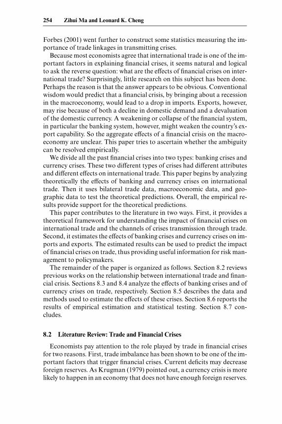
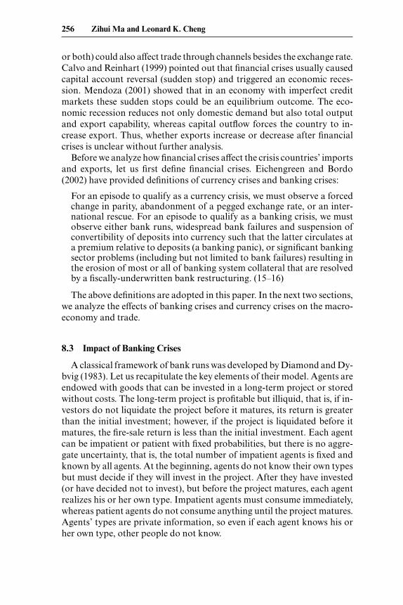
The first two columns of table 8.3 show that the impact of banking criseswas unclear between 1982 and 1990. The short-term effects on imports andexports were insignificant, and the longer-term effects were negative butnot always significant. The results for 1991–1998 were more significant.Imports decreased significantly in all three years. Exports increased in thecrisis years but fell back in the first year after banking crisis.

Impulse response functions induced by the banking crisis dummy arepresented in figures 8.5 and 8.6. We focus on the results for 1991–1998 infigure 8.6. The impact on imports not only was negative but also tended todecrease further.

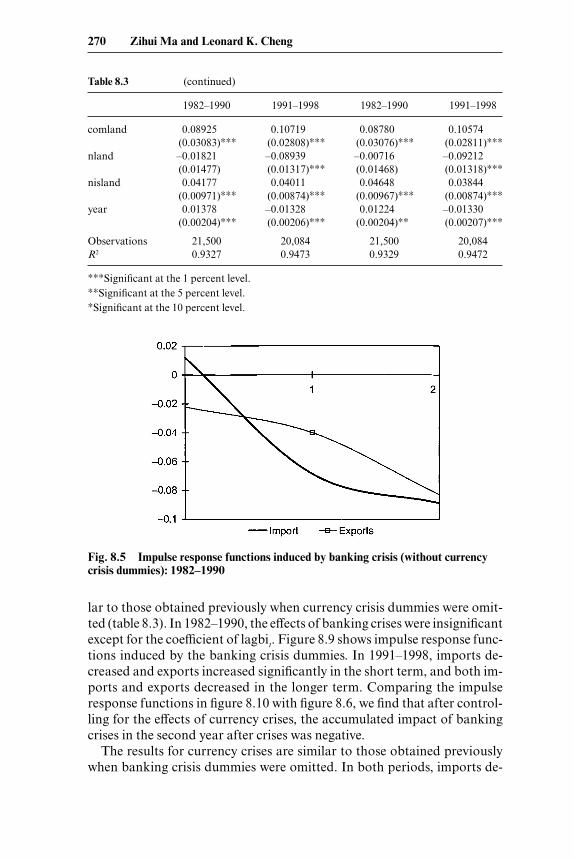
The last two columns of table 8.3 show the effects of currency crises, andthe impulse response functions induced by the currency crisis dummies areshown in figures 8.7 and 8.8. From the table and figures, we find that theeffects on imports in the two periods were very similar. In both periods,imports decreased in all three years. However, the effects on exports in thetwo periods were somewhat different. In 1982–1990, there was a significantnegative impact of currency crises on exports in the short term (i.e., the co-efficients of cet and lagcet–1 were significantly negative), and the negativeimpact was mitigated but not reversed in the second year after crises. Instark contrast, the effects of currency crises on exports in 1991–1998 weresignificantly positive in all three years.

When all crisis dummies are included as explanatory variables, the re-sults are reported in table 8.4. The results for banking crises are very simi-


Table 8.3 Estimation results with separate crisis dummies

1982–1990 1991–1998 1982–1990 1991–1998

Lag export 0.86976 0.86851 0.86849 0.86890(0.00323)∗∗∗ (0.00318)∗∗∗ (0.00323)∗∗∗ (0.00319)∗∗∗

igdp 0.13149 0.11327 0.12863 0.10831(0.00533)∗∗∗ (0.00480)∗∗∗ (0.00538)∗∗∗ (0.00484)∗∗∗

egdp 0.15080 0.13190 0.15098 0.13325(0.00585)∗∗∗ (0.00522)∗∗∗ (0.00586)∗∗∗ (0.00526)∗∗∗

ipop –0.01478 –0.00371 –0.01154 –0.00109(0.00434)∗∗∗ (0.00376) (0.00436)∗∗∗ (0.00383)

epop 0.03950 –0.00734 –0.03819 –0.01016(0.00446)∗∗∗ (0.00378)∗ (0.00447)∗∗∗ (0.00386)∗∗∗

idev –0.18671 –0.06225 –0.16387 –0.07087(0.01426)∗∗∗ (0.02115)∗∗∗ (0.01501)∗∗∗ (0.02141)∗∗∗

edev –0.04301 –0.06271 –0.03050 –0.05268(0.01421)∗∗∗ (0.02124)∗∗∗ (0.01494)∗∗ (0.02147)∗∗∗

lagidev –0.05899 –0.01953 –0.05678 –0.02099(0.01718)∗∗∗ (0.01871) (0.01830)∗∗∗ (0.01927)

lagedev 0.06568 0.05136 0.07026 0.05198(0.01711)∗∗∗ (0.01877)∗∗∗ (0.01825)∗∗∗ (0.01928)∗∗∗

lag2idev 0.19066 0.08434 0.19057 0.09188(0.02039)∗∗∗ (0.01346)∗∗∗ (0.02114)∗∗∗ (0.01374)∗∗∗

lag2edev –0.02843 –0.03143 –0.03533 –0.05060(0.02021) (0.01344)∗∗ (0.02099)∗ (0.01367)∗∗∗

bi 0.01191 –0.12165(0.02405) (0.02079)∗∗∗

be –0.02214 0.10471(0.02382) (0.02077)∗∗∗

lagbi –0.07878 –0.08646(0.02238)∗∗∗ (0.02183)∗∗∗

lagbe –0.02052 –0.01553(0.02231) (0.02208)

lag2bi –0.02929 –0.04187(0.02294) (0.02201)∗

lag2be –0.04835 –0.06378(0.02293)∗∗ (0.02227)∗∗∗

ci –0.09436 –0.07649(0.01609)∗∗∗ (0.01446)∗∗∗

ce –0.07407 0.03537(0.01617)∗∗∗ (0.01441)∗∗

lagci –0.07638 –0.08108(0.01583)∗∗∗ (0.01498)∗∗∗

lagce –0.04656 0.04742(0.01595)∗∗∗ (0.01496)∗∗∗

lag2ci –0.00918 –0.03020(0.01551) (0.01512)∗∗

lag2ce 0.03137 0.02885(0.01558)∗∗ (0.01521)∗

dis –0.12227 –0.11668 –0.12028 –0.11711(0.00512)∗∗∗ (0.00702)∗∗∗ (0.00766)∗∗∗ (0.00704)∗∗∗

(continued )

lar to those obtained previously when currency crisis dummies were omit-ted (table 8.3). In 1982–1990, the effects of banking crises were insignificantexcept for the coefficient of lagbit. Figure 8.9 shows impulse response func-tions induced by the banking crisis dummies. In 1991–1998, imports de-creased and exports increased significantly in the short term, and both im-ports and exports decreased in the longer term. Comparing the impulseresponse functions in figure 8.10 with figure 8.6, we find that after control-ling for the effects of currency crises, the accumulated impact of bankingcrises in the second year after crises was negative.

The results for currency crises are similar to those obtained previouslywhen banking crisis dummies were omitted. In both periods, imports de-


Table 8.3 (continued)

1982–1990 1991–1998 1982–1990 1991–1998

comland 0.08925 0.10719 0.08780 0.10574(0.03083)∗∗∗ (0.02808)∗∗∗ (0.03076)∗∗∗ (0.02811)∗∗∗

nland –0.01821 –0.08939 –0.00716 –0.09212(0.01477) (0.01317)∗∗∗ (0.01468) (0.01318)∗∗∗

nisland 0.04177 0.04011 0.04648 0.03844(0.00971)∗∗∗ (0.00874)∗∗∗ (0.00967)∗∗∗ (0.00874)∗∗∗

year 0.01378 –0.01328 0.01224 –0.01330(0.00204)∗∗∗ (0.00206)∗∗∗ (0.00204)∗∗ (0.00207)∗∗∗

Observations 21,500 20,084 21,500 20,084R2 0.9327 0.9473 0.9329 0.9472

∗∗∗Significant at the 1 percent level.∗∗Significant at the 5 percent level.∗Significant at the 10 percent level.

Fig. 8.5 Impulse response functions induced by banking crisis (without currencycrisis dummies): 1982–1990

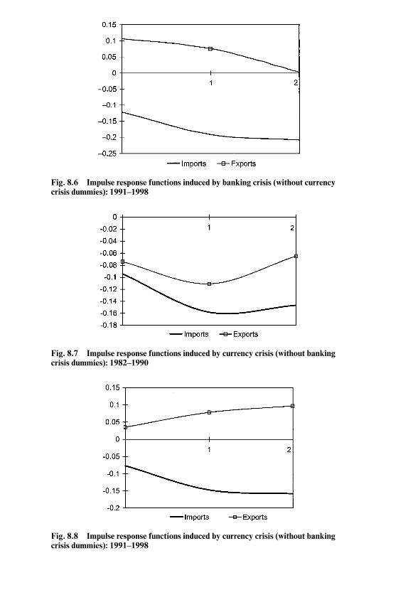
Fig. 8.6 Impulse response functions induced by banking crisis (without currencycrisis dummies): 1991–1998

Fig. 8.7 Impulse response functions induced by currency crisis (without bankingcrisis dummies): 1982–1990

Fig. 8.8 Impulse response functions induced by currency crisis (without bankingcrisis dummies): 1991–1998

Table 8.4 Estimation results with both kinds of crisis

1982–1990 1991–1998

Lag export 0.86863 0.86844(0.00323)∗∗∗ (0.00318)∗∗∗

igdp 0.12788 0.10963(0.00538)∗∗∗ (0.00485)∗∗∗

egdp 0.15057 0.13468(0.00587)∗∗∗ (0.00527)∗∗∗

ipop –0.01186 0.0060652(0.00436)∗∗∗ (0.00384)

epop –0.03861 –0.01081(0.00447)∗∗∗ (0.00387)∗∗∗

idev –0.16730 –0.06468(0.01516)∗∗∗ (0.02145)∗∗∗

edev –0.02874 –0.05658(0.01509)∗ (0.02153)∗∗∗

lagidev –0.04889 –0.01034(0.01846)∗∗∗ (0.01951)

lagedev 0.07141 0.04303(0.01842)∗∗∗ (0.01955)∗∗

lag2idev 0.18519 0.08749(0.02121)∗∗∗ (0.01396)∗∗∗

lag2edev –0.03832 –0.03564(0.02106)∗ (0.01392)∗∗∗

bi 0.00727 –0.09415(0.02414) (0.02212)∗∗∗

be –0.02139 0.09248(0.02391) (0.02210)∗∗∗

lagbi –0.07255 –0.05597(0.02267)∗∗∗ (0.02255)∗∗

lagbe –0.01203 –0.03449(0.02259) (0.02286)

lag2bi –0.00815 –0.02217(0.02318) (0.02234)

lag2be –0.03053 –0.07947(0.02319) (0.02261)∗∗∗

ci –0.08686 –0.04932(0.01632)∗∗∗ (0.01553)∗∗∗

ce –0.07142 0.01902(0.01641)∗∗∗ (0.01548)

lagci –0.07985 –0.06788(0.01599)∗∗∗ (0.01535)∗∗∗

lagce –0.04558 0.05128(0.01611)∗∗∗ (0.01535)∗∗∗

lag2ci –0.01080 –0.03417(0.01560) (0.01528)∗∗∗

lag2ce 0.02943 0.04003(0.01568)∗ (0.01538)∗∗∗

dis –0.11827 –0.11733(0.00770)∗∗∗ (0.00704)∗∗∗

comland 0.09122 0.10606(0.03078)∗∗∗ (0.02808)∗∗∗

nland –0.01102 –0.09101(0.01477) (0.01317)∗∗∗


1982–1990 1991–1998

nisland 0.04454 0.03987(0.00971)∗∗∗ (0.00875)∗∗∗

year 0.01150 –0.01366(0.00205)∗∗∗ (0.00207)∗∗∗

Observations 21,500 20.084R2 0.9329 0.9474


Fig. 8.9 Impulse response functions induced by banking crisis (with currency crisisdummies): 1982–1990

Fig. 8.10 Impulse response functions induced by banking crisis (with currency cri-sis dummies): 1991–1998

creased in all three years. The impact of currency crises on exports was sig-nificant except that during the crisis years in 1982–1990. The impulse re-sponse functions for the currency crisis dummy during the two periods aregiven in figures 8.11 and 8.12, respectively. In 1982–1990, exports de-creased in the short term and remained below the original level despite asubsequent recovery. In 1991–1998, the short-term effect on exports was in-significant, and exports exceeded the original level beginning in the firstyear after currency crises. After controlling the effects of banking crises,the impact of currency crises on exports was insignificant during the crisisyears. So the significantly positive coefficient of cet in table 8.3 seems to bethe result of omitting the banking crisis dummies.

We summarize the theoretical predictions and empirical results about


Fig. 8.11 Impulse response functions induced by currency crisis (with banking cri-sis dummies): 1982–1990

Fig. 8.12 Impulse response functions induced by currency crisis (with banking cri-sis dummies): 1991–1998

the impact of banking crises and currency crises in tables 8.5 and 8.6, re-spectively. Because the model includes GDP and devaluation as explana-tory variables, the effects of the crisis dummies capture the effects of crisesthrough channels other than economic recession or currency devaluation.Theoretical analysis predicts that exports increase during banking crisesdue to foreign outflow, and in the longer term, changes in exports dependon the aggregate effect through the foreign capital flow channel and the in-vestment demand channel; imports would decrease due to reduction in in-vestment demand.

In 1982–1990, the empirical results for banking crises do not support thetheoretical predictions. In particular, there was no increase in exports dur-ing banking crises. Perhaps the theoretical predictions were inappropriatefor this period because many developing countries stopped repaying for-eign debts when they struggled with the financial crises. Furthermore, theamount of foreign capital flow into less-developed economies was rela-tively modest.

The empirical results for 1991–1998 were broadly consistent with theo-retical predictions. The negative longer-term effect of banking crises on im-ports is as predicted. Although the theories predict the short-term effect on


Table 8.5 The effects of banking crisis on trade

Theoretical prediction

Empirical resultsForeign Investment Aggregate Income capital flow demand effects (except channel channel channel income channel) 1982–1990 1991–1998

Imports (short) – ? ? –Imports (longer) – – – ? –Exports (short) – � � ? �

Exports (longer) – – � ? ? –

Notes: Dash � negative; plus sign � positive; question mark � unclear or insignificant.

Table 8.6 The effects of currency crisis on trade


Empirical resultsMarket Substitution Aggregate chaos Income effect Wealth effects (except

channel channel channel channel income channel) 1982–1990 1991–1998

Imports (short) – – – –Imports (longer) – – – – – –Exports (short) – – – ?Exports (longer) – – � ? –a �

Notes: See table 8.5 notes.aThe accumulated effect was negative but tended to increase.

imports to be insignificant, the empirical negative impact on imports dur-ing crisis years may be due to the use of annual data (as opposed to quar-terly or monthly data), which might have been influenced by the longer-term effects. The positive impact on exports in the short term is consistentwith the theoretical prediction about the effect of capital outflow. The re-sults that exports decreased in the longer term (the second year after crisis)implies that the negative effect via the capital flow channel overwhelmedthe positive effect through the investment demand channel.

Theoretical analysis predicts that currency crises had negative impact onimports both in the short term (due to market chaos) and the longer term(due to wealth loss plus substitution effect if crisis was triggered by exter-nal shocks). The short-term effect on exports are negative, but the longer-term effect was ambiguous because the positive effect via the wealth chan-nel ran counter to the negative effect via the substitution effect if the crisiswas triggered by external shocks.

Comparing the empirical results of currency crises with the theoreticalpredictions, we discover three phenomena. First, consistent with theoreti-cal predictions, the impact of currency crises on imports were negative inboth the short term and the longer term. Second, the short-term effect viathe market chaos channel in 1991–1998 was weaker than that in 1982–1990,so exports decreased significantly in crisis years in 1982–1990 but did notchange significantly in 1991–1998. Third, in 1982–1990, exports after thecrisis recovered but still remained below the original level. We are not cer-tain whether it was due to a weakening of the short-term effect or if thelonger-term effect had kicked in. In contrast, in 1991–1998, exports in-creased significantly after currency crises, implying that the impact via thewealth channel overwhelmed the impact through the substitution effectchannel. Generally, the empirical results in both periods are broadly con-sistent with theoretical predictions.

8.6.3 Twin Crises, Successful and Unsuccessful Crises

Let us check for the effects of twin crises by adding a twin crisis dummy,tct � bit � cit, and its first and second lags. Clearly tcit � 1 if and only ifboth bit and cit are equal to 1.

The estimation results are listed in table 8.7. Most coefficients of the twincrisis dummy variables are insignificant even though the values of the co-efficients are not small in relative terms.

As we pointed out previously, currency crises may be “successful” or“unsuccessful.” Because currency devaluations did not occur in unsuc-cessful currency crises, their impact could be different from that of suc-cessful crises. We separate the currency crisis dummies into two more re-fined groups of variables: sc stands for a successful currency crisis (i.e.,both currency crisis and devaluation happen); fc stands for an unsuccess-ful currency crisis (i.e., a currency crisis without devaluation). The results


Table 8.7 Estimation results with twin crisis dummies

1982–1990 1991–1998

Lag export 0.86877 0.86833(0.00323)∗∗∗ (0.00319)∗∗∗

igdp 0.12765 0.10960(0.00539)∗∗∗ (0.00486)∗∗∗

egdp 0.15061 0.13460(0.00588)∗∗∗ (0.00528)∗∗∗

ipop –0.01171 0.00089734(0.00436)∗∗ (0.00386)

epop –0.03865 –0.01044(0.00447)∗∗∗ (0.00389)∗∗∗

idev –0.15667 –0.06641(0.01608)∗∗∗ (0.02161)∗∗∗

edev –0.02151 –0.05560(0.01599) (0.02235)∗∗

lagidev –0.06552 –0.01134(0.02035)∗∗∗ (0.01960)

lagedev 0.06187 0.04110(0.02025)∗∗∗ (0.01991)∗∗

lag2idev 0.19037 0.08756(0.02133)∗∗∗ (0.01407)∗∗∗

lag2edev –0.03601 –0.03680(0.02118)∗ (0.01405)∗∗∗

bi 0.01752 –0.08838(0.02575) (0.03191)∗∗∗

be –0.00993 0.10311(0.02551) (0.01825)∗∗∗

lagbi –0.08615 –0.06949(0.02356)∗∗∗ (0.03000)∗∗

lagbe –0.02074 –0.03919(0.02350) (0.03070)

lag2bi 0.00052686 –0.02985(0.02373) (0.02743)

lag2be –0.03660 –0.09457(0.02376) (0.02784)∗∗∗

ci –0.08610 –0.04906(0.01643)∗∗∗ (0.01673)∗∗∗

ce –0.06722 0.02059(0.01653)∗∗∗ (0.01613)

lagci –0.08321 –0.07232(0.01607)∗∗∗ (0.01629)∗∗∗

lagce –0.04637 0.04860(0.01620)∗∗∗ (0.01631)∗∗∗

lag2ci –0.00878 –0.03609(0.01570) (0.01617)∗∗

lag2ce 0.02657 0.03514(0.01578)∗ (0.01628)∗∗

tci –0.07250 –0.01222(0.07379) (0.04424)

(continued )

are reported in table 8.8. Because most currency crises were successful, it isnot surprising that the coefficients of sc are close to those of c in table 8.4.We find that the longer-term effects of unsuccessful currency crises wereunclear: almost all coefficients of lagfc and lag2fc are insignificant. How-ever, the short-term effects of unsuccessful crises in the two periods weredifferent. In 1982–1990, imports did not change significantly, but exportsdecreased significantly after an unsuccessful currency crisis. However, in1991–1998, an unsuccessful currency had negative effects on imports butpositive effects on exports. Most of the other coefficients were not affectedby the separation into two different currency crisis variables.

8.6.4 How Large are the Effects on Trade?

Because the variables are expressed in logarithmic terms, we can com-pute the size of the effects from the regression results contained in tables8.5 and 8.6 and by using the impulse response functions in figures 8.9, 8.10,8.11, and 8.12. In 1991–1998, a country’s imports on average would declineby about 9.7 percent during the year in which a banking crisis occurred, by



1982–1990 1991–1998

tce –0.08419 –0.02618(0.07263) (0.04281)

lagtci 0.17891 0.03273(0.09067)∗∗ (0.04514)

lagtce 0.10041 0.01055(0.08874) (0.04540)

lag2tci –0.13564 0.02193(0.11350) (0.04579)

lag2tce 0.16103 0.04215(0.12235) (0.04627)

dis –0.11825 –0.11755(0.00770)∗∗∗ (0.00705)∗∗∗

comland 0.09047 0.10623(0.03078)∗∗∗ (0.02808)∗∗∗

nland –0.01042 –0.09064(0.01478) (0.01321)∗∗∗

nisland 0.04481 0.04019(0.00971)∗∗∗ (0.00878)∗∗∗

year 0.01148 –0.01389(0.00207)∗∗∗ (0.00210)∗∗∗

Observations 21,500 20,084R2 0.933 0.9474


Table 8.8 Estimation results with both “successful” and “unsuccessful” currencycrisis dummies

1982–1990 1991–1998

Lag export 0.86855 0.86796(0.00324)∗∗∗ (0.00320)∗∗∗

igdp 0.12621 0.11027(0.00547)∗∗∗ (0.00488)∗∗∗

egdp 0.15203 0.13519(0.00598)∗∗∗ (0.00530)∗∗∗

ipop –0.01021 0.00029741(0.00443)∗∗ (0.00385)

epop –0.03987 –0.01036(0.00456)∗∗∗ (0.00388)∗∗∗

idev –0.16159 –0.06904(0.01536)∗∗∗ (0.02209)∗∗∗

edev –0.02700 –0.04247(0.01528)∗ (0.02218)∗

lagidev –0.04797 –0.00798(0.01872)∗∗ (0.01975)

lagedev 0.07718 0.03514(0.01865)∗∗∗ (0.01978)∗

lag2idev 0.18412 0.08705(0.02152)∗∗∗ (0.01400)∗∗∗

lag2edev –0.05234 –0.03529(0.02136)∗∗ (0.01395)∗∗

bi 0.00495 –0.09108(0.02417) (0.02233)∗∗∗

be –0.02285 0.08417(0.02395) (0.02231)∗∗∗

lagbi –0.07791 –0.05444(0.02281)∗∗∗ (0.02268)∗∗

lagbe –0.00509 –0.04039(0.02274) (0.02298)∗

lag2bi –0.00653 –0.02153(0.02327) (0.02238)

lag2be –0.03390 –0.08059(0.02329) (0.02265)∗∗∗

sci –0.10246 –0.04392(0.01748)∗∗∗ (0.01641)∗∗∗

sce –0.06925 0.00505(0.01757)∗∗∗ (0.01636)

lagsci –0.08581 –0.06681(0.01741)∗∗∗ (0.01585)∗∗∗

lagsce –0.05739 0.05068(0.01751)∗∗∗ (0.01586)∗∗∗

lag2sci –0.01370 –0.03521(0.01704) (0.01570)∗∗

lag2sce 0.05255 0.04344(0.01709)∗∗∗ (0.01580)∗∗∗

(continued )

13 percent in the first year after crises, by 14.5 percent in the subsequentyear; exports would increase by about 8.8 percent during the crisis year, by5 percent in the first year after crisis, but would decrease by 2 percent in thesecond year after crisis. The country’s imports would drop by about 4.3percent during the year in which a successful currency crisis occurred, by9.7 percent and 12.4 percent in the subsequent two years, respectively; ex-ports would increase by about 0.5 percent (insignificant) during the crisisyear, by about 5 percent and 9 percent in the two subsequent years aftercrises, respectively. The results show that the impact of financial crises oninternational trade was very strong.

8.7 Conclusions and Directions for Further Research

We have analyzed how financial crises affected international trade in thelast two decades, an important question largely ignored by the literature.Our theoretical analysis predicts that imports will decrease during and af-



1982–1990 1991–1998

fci 0.01289 –0.08822(0.04149) (0.04050)∗∗

fce –0.10889 0.11401(0.04199)∗∗∗ (0.04028)∗∗∗

lagfci –0.05894 –0.06386(0.03678) (0.06416)

lagfce 0.01192 –0.00087749(0.03759) (0.06417)

lag2fci 0.01488 –0.00998(0.03678) (0.06430)

lag2fce –0.08725 –0.00735(0.03752)∗∗ (0.06431)

dis –0.011826 –0.11804(0.00770)∗∗∗ (0.00705)∗∗∗

comland 0.09110 0.10594(0.03077)∗∗∗ (0.02808)∗∗∗

nland –0.01006 –0.09101(0.01485) (0.01318)∗∗∗

nisland 0.04415 0.04004(0.00971)∗∗∗ (0.00876)∗∗∗

year 0.01141 –0.01402(0.00206)∗∗∗ (0.00214)∗∗∗

Observations 21,500 20,084R2 0.933 0.9474


ter a banking crisis, whereas exports will rise during but fall after the crisis.Theoretical analysis predicts imports and exports will fall during currencycrises, but the effect after the crisis depends on the source of externalshocks. By estimating a model of bilateral trade between fifty countriesover a period of nineteen years with real-world data, we have found that theempirical results are generally consistent with the theoretical predictions,especially in 1991–1998. The empirical results also show that after cur-rency crises exports increased more significantly in 1991–1998 than in1982–1990. That may be a clue of “contagious crisis” in the last decade.

This paper has focused on the value of trade, but an alternative measurewould be the volume of trade. In addition, the impact of financial crises ondifferent tradable goods may be different. It would be interesting to explorewhether the relationships between trade and financial crisis varied system-atically across different products. For instance, products that enjoyed a com-parative advantage versus those that suffered a comparative disadvantage.Another possible direction for future research is the effects of economicstructures and government policies on trade. We found that the impact of fi-nancial crises was different between the 1980s and 1990s. Whether and howmuch of this difference was attributable to differences in economic struc-tures and government policies seems to be a worthwhile topic to explore.

References

Baig, Taimur, and Ilan Goldfajn. 1998. Financial market contagion in the Asiancrisis. International Monetary Fund Working Paper no. WP/98/155. Washing-ton, DC: IMF, November.

Calvo, Guillermo A., and Carmen M. Reinhart. 1999. When capital inflows cometo a sudden stop: Consequences and policy options. Working Paper, June.

Diamond, Douglas W., and Philip H. Dybvig. 1983. Bank runs, deposit insurance,and liquidity. Journal of Political Economy 91:401–19.

Eichengreen, Barry, and Michael D. Bordo. 2002. Crises now and then: What les-sons from the last era of financial globalization? NBER Working Paper no. 8716.Cambridge, MA: National Bureau of Economic Research.

Eichengreen, Barry, and Andrew K. Rose. 1999. Contagious currency crises: Chan-nels of conveyance. In Changes in exchange rates in rapidly developing countries:Theory, practice, and policy issues, ed. Takatoshi Ito and Anne O. Krueger, 29–50. Chicago: University of Chicago Press.

Eichengreen, Barry, Andrew K. Rose, and Charles Wyplosz. 1996. Contagious cur-rency crises. NBER Working Paper no. 5681. Cambridge, MA: National Bureauof Economic Research, July.

Frankel, Jeffrey, and Andrew K. Rose. 2002. An estimate of the effect of currencyunions on trade and income. Quarterly Journal of Economics 117 (2): 437–66.

Forbes, Kristin. 2000. The Asian flu and Russian virus: Firm level evidence on howcrises are transmitted internationally. NBER Working Paper no. 7807. Cam-bridge, MA: National Bureau of Economic Research, July.


———. 2001. Are trade linkages important determinants of country vulnerabilityto crises? NBER Working Paper no. 8194. Cambridge, MA: National Bureau ofEconomic Research, March.

Glick, Reuven, and Andrew K. Rose. 1999. Contagion and trade: Why are currencycrises regional? Journal of International Money and Finance 18:603–17.

Kaminsky, Graciela L., and Carmen M. Reinhart. 1999. The twin crises: Thecauses of banking and balance-of-payments problems. American Economic Re-view 89:473–500.

Krugman, Paul. 1979. A model of balance of payments crises. Journal of Money,Credit and Banking 11:311–25.

Masson, Paul. 1998. Contagion: Monsoonal effects, spillovers, and jumps betweenmultiple equilibria. International Monetary Fund Working Paper no. WP/98/142. Washington, DC: IMF, September.

Mendoza, Enrique G. 2001. Credit, prices, and crashes: Business cycles with a sud-den stop. NBER Working Paper no. 8338. Cambridge, MA: National Bureau ofEconomic Research, June.

Obstfeld, Maurice. 1996. Models of currency crises with self-fulfilling features. Eu-ropean Economic Review 40:1037–47.

Comment Chin Hee Hahn

It has been recognized in the previous literature that financial crises have a“contagious effect.” While the focus of several preceding studies was onwhether trade linkage plays a role in transmitting crises across countries,this paper examines more closely how financial crises affect exports andimports. Insofar as understanding the effects of financial crises on tradeflows is complementary to understanding the role of trade in transmittingcrises, this paper raises a very important question. To address this ques-tion, this paper provides an outline of the theoretical framework as well asan empirical analysis. I think this paper is a serious attempt to add to theliterature on the effects and transmission of financial crises.

Nevertheless, the specification of the regressions doesn’t seem to allowus to interpret the empirical results clearly. Because the basic regressionmodel includes gross domestic product (GDP) and devaluation variables,the estimated coefficients on crisis dummy variables and, hence, the im-pulse responses of trade flows to crises would capture the effect of crises ontrade that is not captured by changes in the GDP or the exchange rate.However, financial crises are likely to affect trade mostly by affecting theGDP or the exchange rate. The theoretical framework in this paper alsosuggests that this is likely to be the case. Then, what interpretation we cangive to the coefficients on crisis variables and, hence, to the impulse re-sponses, seems to be somewhat unclear. For example, if there is less foreign


Chin Hee Hahn is a research fellow of the Korea Development Institute.

capital inflow after a banking crisis to finance domestic investment proj-ects, then it is likely to affect the GDP or the exchange rate or both, at leastin the short term. Then, the estimated effect of a banking crisis on trade,controlling for the GDP and changes in the exchange rate, is likely to cap-ture those effects of the banking crisis that is not associated with changesin the GDP or the exchange rate. At least, the theoretical framework in thispaper does not tell us clearly what these effects are. Viewed from this per-spective, the estimated magnitudes of the effects of crises on trade flowsseem to be very large. For example, a banking crisis reduces imports byabout 12 percent during the crisis year, and by about 20 percent cumula-tively during the three-year period after the crisis, with these effects not as-sociated with changes in the GDP or the exchange rate.

Comment Kozo Kiyota

This paper examines the impacts of banking and financial crises on inter-national trade both theoretically and empirically. Hypotheses drawn fromthe theoretical analyses are in table 8C.1. The aggregated effects of a bank-ing crisis on exports (except income channel) are positive in the short termwhile those on imports are negative in the long term. On the other hand, allaggregated impacts of currency crises on international trade except long-term exports are negative.

To test these hypotheses, the authors estimated a gravity model withbanking and currency crises dummies, using data for fifty countries from1982 to 1998. As table 8C.1 shows, the empirical analysis generally sup-ports the theoretical prediction. The short-run impacts of currency criseson exports are positive for the period 1982–1990. On the other hand, forthe period 1991–1998, currency crises had negative impacts on imports inthe short and long terms. In addition, the analysis confirmed that bankingcrises had negative impacts on imports in the short term but positive im-pacts on exports in the long term. The authors also examined the scale ofthese impacts on international trade using an impulse-response functionand found that these impacts were significantly strong.

The question addressed in this paper is one of the most important issuesin analyzing the impacts of financial crises. The paper has three importantfindings. First, the channels and impacts of banking crises on internationaltrade are different from those of currency crises. Second, the impacts of thecrises are different between the short and long terms. Finally, the impactsof crises are different between the 1980s and the 1990s. This is an excellent


Kozo Kiyota is associate professor in the faculty of business administration at YokohamaNational University.

paper with important policy implications. However, there is some room forimprovement, which is summarized as follows.

1. In the currency crises model, the different impacts between short andlong terms are not very clear. For instance, why does the income channelwork only for the long term in a currency crisis while it works for both theshort and long term in a banking crisis? Because the different impacts be-tween the short and long terms is one of the important findings of this pa-per, further explanation of the difference would be helpful.

2. The authors investigate the effects of twin crises. However, they offerno explanation about the interaction between banking and currency crisesin their theoretical analysis. Therefore, the expected impacts of twin crisesare not clear. The empirical analysis employs a dummy variable that is de-fined as the cross term of banking and financial crises dummies. This is also


Table 8C.1 The effects of banking and currency crises on trade: Theoretical prediction andempirical results

The effects of banking crises on trade


Empirical resultsForeign Investment Aggregate Income capital flow demand effects (except channel channel channel income channel) 1982–1990 1991–1998

ImportsShort term – ? ? –Long term – – ? –a

ExportsShort term – � � ? �a

Long term – – � ? ? –

The effects of currency crises on trade


Empirical resultsMarket Substitution Aggregate chaos Income effect Wealth effects (except

channel channel channel channel income channel) 1982–1990 1991–1998

ImportsShort term – – –a –a

Long term – – – – –a –a

ExportsShort term – – –a –a

Long term – – � ? – �

Sources: Tables 8.5 and 8.6.Notes: Dash � negative; plus sign � positive; question mark � unclear or insignificant.aEmpirical results support theoretical prediction.

difficult to interpret because the cross term can reflect several combina-tions of the impacts (for instance, positive signs are obtained whenever theimpacts of two crises are the same despite each coefficient of crises beingpositive or negative). Similarly, the authors do not provide any explanationabout the expected impacts of “successful” and “unsuccessful” crises.This, in turn, implies that it is hard to interpret the estimation results. Theauthors could therefore provide some discussion of the expected effects oftwin crises and “successful” and “unsuccessful” crises in their theoreticalsection.

3. The authors should provide more information about their empiricalmethodology. It is not clear whether their regression analysis employed apanel-data method such as a random-effect model. Further, the authorsshould present such basic indicators as the mean, variance, and correlationmatrix of the variables. Such information could help to determine if someof the insignificant results might be caused by an inappropriate estimationmethod, specification error, or multicollinearity of independent variables.

4. This paper uses annual data in the empirical analysis. However, bank-ing and currency crises may occur rapidly. Therefore, annual data mightnot capture some of the important impacts on international trade. If dataare available, quarterly or monthly data would be more appropriate to cap-ture the impacts of the crises.

5. The authors found that the impact of financial crises was different be-tween the 1980s and 1990s. This is an interesting finding. More useful in-formation could be obtained if the authors reported table 8.1 separately forthe 1980s and the 1990s. That is, were the same countries affected in boththe 1980s and the 1990s, or did countries face changes after 1990? Simplemodification of table 8.1 might provide much helpful information.

6. There are several extensions of the research that could be pursued, in-cluding the impacts of financial crises on comparative advantage, intrare-gional trade, intraindustry trade, and intrafirm trade. Among these topics,the effects of banking and financial crises on intraregional trade could bean especially interesting topic. Because financial crises tend to be regional(Glick and Rose 1999), such analysis might also reveal the different im-pacts between banking and financial crises.

Reference

Glick, Reuven, and Andrew K. Rose. 1999. Contagion and trade: Why are currencycrises regional? Journal of International Money and Finance 18:603–17.


the effects of financial crises on international trade · zihui ma is lecturer of international...

Documents