The Ralph & Goldy Lewis Center for Regional Policy Studies at UCLA...established to promote the study, understanding and solution of regional policyissues, with special reference to Southern California, including problems of theenvironment, urban design, housing, community and neighborhood dynamics,transportation and economic development...

Working Paper Series

The Effects of Free Parking on Commuter Mode Choice: Evidence from Travel Diary Data

By: Daniel Baldwin Hess

Working Paper #34 in the series

The Ralph & Goldy Lewis Center for Regional Policy StudiesUCLA, School of Public Policy and Social Research

3250 Public Policy BuildingLos Angeles CA 90095-1656

Director: Paul OngPhone: (310) 206-4417Fax: (310) 825-1575

http://www.sppsr.ucla.edu/lewis/April 2001

Disclaimer: Neither the University of California, the School of Public Policy and Social Research nor the Lewis Center for Regional PolicyStudies either support or disavow the findings in any project, report, paper, or research listed herein. University affiliations are foridentification only; the University is not involved in or responsible for the project.

THE EFFECT OF FREE PARKING ON COMMUTER MODE CHOICE:EVIDENCE FROM TRAVEL DIARY DATA

Daniel Baldwin HessInstitute of Transportation Studies

University of California, Los Angeles3250 Public Policy Building, Box 951656

Los Angeles, California, 90095-1656e-mail dhess@ucla.edu

ABSTRACT

This study assesses the effect of free parking on mode choice and parking demand. A multinomiallogit model is developed to evaluate the probabilities that commuters who do and who do not receivefree parking at work will choose to drive alone, ride in a carpool, or use transit for the trip to workin Portland’s (Oregon) CBD. The mode choice model predicts that with free parking, 62 percent ofcommuters will drive alone, 16 percent will commute in carpools and 22 percent will ride transit;with a daily parking charge of $6, 46 percent will drive alone, 4 percent will ride in carpools and 50percent will ride transit. The mode choice model predicts that a daily parking charge of $6 in thePortland CBD would result in 21 fewer cars driven for every 100 commuters. This translates to adaily reduction of 147 VMT per 100 commuters and an annual reduction of 39,000 VMT per 100commuters. These findings are consistent with previous studies of the effect of parking cost on modechoice. The policy variables that play a part in mode choice decisions for commuters are the parkingcost and the travel time by transit, and the results suggest that raising the cost of parking at work sitesand decreasing the transit travel time (by improving service and decreasing headways) will reducethe drive alone mode share. The results provide little support for the contention that land use is asignificant factor in mode choice decisions.

Key words: parking, mode choice, activity survey, modeling, commuting

AcknowledgmentsThe author would like to acknowledge support for this project from the Graduate Division, University of California, Los Angeles.Special thanks go to Jeffrey Brown, Dan Chatman, Paul M. Ong, Lisa Schweitzer, Donald Shoup, and Richard Willson for providinghelpful comments

1

Introduction

When commuters can park their cars free at work, they are more likely to drive alone.

American employers provide 85 million free parking spaces for commuters. Approximately 91

percent of commuters in the U.S. drive to work, and 92 percent of the cars driven to work have only

one occupant (Shoup 1999).1 Using data from the 1990 Nationwide Personal Transportation Survey

(NPTS), Shoup (1995) estimated that parking is free to the driver for 95 percent of automobile work

trips. Employers encourage solo driving to work when they pay part of the cost of the commute trip

— the parking cost — while requiring the employee to pay only the driving cost. This leads to a

significant reduction in the cost of driving to work, thus encouraging more driving. By offering their

employees free parking at work, employers stymie public goals of reducing solo driving and

increasing the use of carpooling, transit, walking, and bicycling for the commute to work.

This study assesses the effect of free parking on mode choice and parking demand. I develop

a model to estimate the probability that commuters who do and who do not receive free parking at

work will choose to drive alone, ride in a carpool, or use transit for the trip to work. The hypothesis

tested is that free parking encourages driving to work — especially in single occupant vehicles. I will

also investigate whether drivers who must pay to park at work are more likely to use an alternative

mode. I use data from a household activity survey to model the interdependence of parking cost and

mode choice. I develop a multinomial logit model of mode choice for the work trip to Portland’s

(Oregon) central business district (CBD) to evaluate and interpret daily commuting behavior.2 Unlike

other mode choice models, the model developed in this study can predict changes in the factors

affecting travel behavior, such as a change in the parking price. The mode choice model predicts that

with free parking, 62 percent of commuters will drive alone, 16 percent will commute in carpools and

22 percent will ride transit; with a daily parking charge of $6, 46 percent will drive alone, 4 percent

will ride in carpools and 50 percent will ride transit.

Development of a Database for Hypothesis Testing

This study uses data from the Oregon and Southwestern Washington 1994 Activity and Travel

Behavior Survey,3 a detailed travel diary that collected data from 4,451 households using a region-

wide, two-day activity survey (Cambridge Systematics 1996). The survey, conducted by the Portland

2

Metropolitan Services District (Portland Metro), recorded what each member in a household did

(activity choice), where (location choice), for how long (activity duration), and with whom (activity

participation). For each activity that required travel, the survey collected detailed information about

the trip.

The survey data consists of 9,471 persons reporting 122,348 activities and 67,981 valid trips.

Activities were grouped into 27 categories.4 Activity/travel data were collected for every household

member, regardless of age. Each household was assigned two consecutive travel days to record

activities for all household members, and the travel days assigned to households were varied to

capture data representing all the days of the week.5 Households were geocoded to transportation

analysis zones (TAZs) in Portland Metro’s 1,260-TAZ system. Table 1 summarizes the households,

trips, and vehicles for each household that participated in the household activity survey.

Table 1 Household and Transportation Activity Estimates

Measure Estimate

Total households6 567,126 households

Average household size 2.3 persons

Average number of vehicles per

household

1.73 vehicles

Total trips recorded (all modes) 67,981 trips

Average trip rate per household per day 8.04 trips

Average activity rate per household per day 14.48 activities

Total activities reported 122,348 activities

Travel volume projection 4,599,693 trips

Source: NuStats International, Inc. 1995. Oregon and Southwest Washington Household Activity and Travel Surveys.

Geographic Stratification of Survey Respondents

One of the primary goals of the Household Activity Survey was to collect data that could be

used to study a variety of transportation-related behavior. The relationship between the built

environment and transportation behavior was of particular interest to Portland Metro, the MPO

3

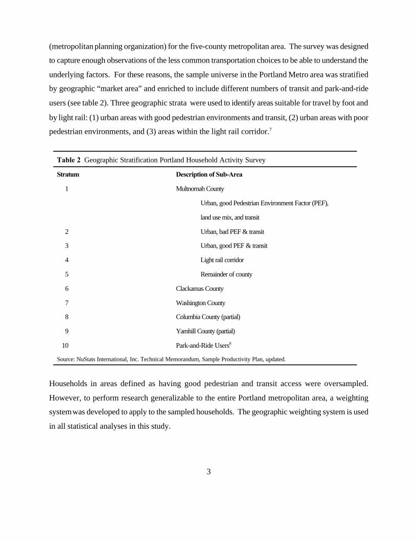
(metropolitan planning organization) for the five-county metropolitan area. The survey was designed

to capture enough observations of the less common transportation choices to be able to understand the

underlying factors. For these reasons, the sample universe in the Portland Metro area was stratified

by geographic “market area” and enriched to include different numbers of transit and park-and-ride

users (see table 2). Three geographic strata were used to identify areas suitable for travel by foot and

by light rail: (1) urban areas with good pedestrian environments and transit, (2) urban areas with poor

pedestrian environments, and (3) areas within the light rail corridor.7

Table 2 Geographic Stratification Portland Household Activity Survey

Stratum Description of Sub-Area

1 Multnomah County

Urban, good Pedestrian Environment Factor (PEF),

land use mix, and transit

2 Urban, bad PEF & transit

3 Urban, good PEF & transit

4 Light rail corridor

5 Remainder of county

6 Clackamas County

7 Washington County

8 Columbia County (partial)

9 Yamhill County (partial)

10 Park-and-Ride Users8

Source: NuStats International, Inc. Technical Memorandum, Sample Productivity Plan, updated.

Households in areas defined as having good pedestrian and transit access were oversampled.

However, to perform research generalizable to the entire Portland metropolitan area, a weighting

system was developed to apply to the sampled households. The geographic weighting system is used

in all statistical analyses in this study.

4

Survey Method

Portland Metro contracted with a survey firm to conduct the Household Activity Survey.9 The

survey firm purchased from a national sampling service a random probability sample of telephone

exchanges from which to recruit households in each geographic strata. Therefore, each household with

a telephone had an equal probability of being included in the sample, whether or not the telephone

number was listed.10

Data collection for the Household Activity Survey included the following steps: (1)

recruitment of household by telephone; (2) mailing survey packets to participating households; (3)

reminder calls to participating households on the day before their designated travel days; and (4)

retrieval of data via telephone interviews after the second designated travel day.

Development of a Database for the Mode Choice Model

The first step was to extract from the household activity survey only those observations that

result in trips that are valid for this study. Of the survey’s 76,939 trips, 25,277 (about one-third) were

designated as work trips (home-based work trips, non home-based work trips, and college trips). Of

these, 2,606 ended at a destination within the Portland CBD11 (see map 1). Of these, 843 trips take

place during the weekday morning peak travel period. Of those, 584 trips are made by solo drivers,

carpoolers, or transit riders. In the end, 523 trips are used to develop the mode choice model after

45 trips are excluded because of missing data.

Descriptive statistics, correlation, and cross-tabulation document the general findings in the mode

choice analysis. The following tables show the demographic distribution of those who park free and

those who pay to park.

Table 3 lists the mode split for all commuters to the Portland CBD during the weekday

morning peak determined from the household activity survey.12 Of those commuters in automobiles,

82 percent are solo drivers, and 18 percent are in vehicles with 2 or more occupants. Slightly more

than half of all commuters drive alone. This display of mode choice is typical of a large CBD with

healthy transit.13

5

Map 1Portland, Oregon CBD

Study Area (in dark gray)

Portland

W il llam ette Riv e r

.-, 5

.-,405

(/84

6

Table 3 Sample Mode Distribution for Commuters to Portland CBD Weekday Morning Peak

Mode Percent of Commuters

Drive alone 50.9 %

Carpool 10.8 %

Transit

Bus 24.5 %

Light rail 3.4 %

Walk 8.3 %

Bicycle 2.1 %

Sum 100.0 %

I now turn to the incidence of free parking among commuters as determined from the household

activity survey. Among solo drivers, just over half of commuters park free regardless of their age,

gender, or income (see table 4). The mode choice outcomes in table 4 closely match the findings from

a separate study of the effects of employer-paid parking by Willson and Shoup (1990) for Los

Angeles.14

Table 4 Free Parking vs. Paid Parking for Solo Commuters, Carpools and Transit Riders

Mode Commuters

Drive alone 54 %

Carpool 14%

Transit 32 %

Total 100 %

53 % of Commuters Park Free

47 % of Commuters Pay to Park

7

In Portland, those who drove to work reported the actual price paid for parking if they did not

park free, and those who rode transit reported the amount they would have paid to park (had they

driven) if there would have been a parking charge. The average price paid to park among the sample

group is $2.00 per day, with a range from $0 to $9. However, the average price paid to park among

those who did not park free is $5.40 per day.

The price paid to park varies among commuters who arrive at the CBD by various modes.

Table 5 lists the average daily parking price paid by those who did or would have had to pay to park

their cars;15 commuters in single occupant vehicles (SOVs) paid $5.17 per day, commuters in

carpools paid $7.66 per day per vehicle (or $3.33 per commuter with a carpool occupancy rate of

2.3), and transit riders paid $6.47 per day. Transit riders had the highest average daily parking charge

and paid an average of 25 percent higher than those who commuted in SOVs.

Table 5 Daily Parking Cost for Commuters to the Portland CBD

Mode Daily parking price

SOV $5.17

Carpool* $7.66 per vehicle

$3.33 per commuter

Transit $6.47

* Assumes carpool occupancy rate of 2.3, the average rate for commuters to the CBD (during the weekday morningpeak period) determined from the 1994 Portland Household Activity Survey.

I can also compare this study’s mode choice outcomes with data from the NPTS. Mildner et

al. (1998) found that only 7.7 percent of drivers paid to park at work (n=44) although 50 percent of

respondents indicated that they lived within 1/4 mile of transit (bus and light rail). Mildner et al.

(1998) define Portland as a transit-accommodating city, where congestion costs are high and transit

ridership may be higher-than-average.16 There are no minimum parking requirements imposed in the

Portland CBD, but there are parking maximums. In the Portland CBD, 10 percent of parking is

publicly owned and the maximum parking meter rate is 90¢ (Mildner et al. 1998).

8

I now consider the distribution of free parking by occupation, using occupational status as a

proxy for income. Occupation classifications from the household activity survey are collapsed into

two categories: managerial/ professional and all others (see table 6).

Table 6 Free Parking and Paid Parking by Occupation Type

Free parking Pay to park Total

Managerial/professional 30 % 28 % 58 %

All other occupations 22 % 20 % 42 %

Total 52 % 48 % 100 %

Commuters in managerial and professional occupations (who constitute the majority of commuters to

Portland’s CBD) are only slightly more likely to receive free parking than commuters in other

occupations.

Finally, I consider the effect of the daily price of parking on mode choice decision (see table

7). The majority of commuters (62.8 percent combined) in single occupant vehicles, in carpools, or

on transit did or would have received employer-paid parking.17 There is no pattern evident in the

relationship between daily parking charge and mode choice among those who parked free and those

who paid to park.18

Table 7 Effect of Parking Cost on Mode Choice

Mode share

Daily Parking Cost Solo driver Carpool Transit

$0 58 % 18 % 24 %

$1 35 % 63 % 2 %

$2 77 % 18 % 5 %

$3 58 % 5 % 37 %

$4 43 % 11 % 46 %

$5 61 % 3 % 36 %

$6 or more 49 % 4 % 47 %

Total 54 % 14 % 32 %

9

Development of a Probabilistic Choice ModelI assume that mode choice for the commute trip is an expression of preferences, and that the

mode choice can be predicted if all of the relevant variables are known. A probabilistic prediction

of choice is an expression of the probabilities that each of the available alternatives will be chosen.

A model that relates these probabilities to the values of a set of explanatory variables is called a

probabilistic choice model (Horowitz 1995).

I can use a multinomial logit model to estimate the influence of variables on the decision to

choose a certain travel alternative.19 I define three dependent variables: P1 (the probability that a

commuter chooses to drive an SOV), P2 (the probability that a commuter chooses to carpool), and P3

(the probability that a commuter chooses transit). By definition, the three probabilities sum to unity:

P P P1 2 3 1+ + =

The fitted regression model is given by two equations:

(Equation A)log ...P

Px x x xa a a a ia i

1

31 1 2 2 3 3

= + + ++ +α β β β β

(Equation B)log ...P

Px x x xb b b b ib i

2

31 1 2 2 3 3

= + + ++ +α β β β β

In these equations, xi (i = 1, 2, 3 ..... n) denotes the attributes of alternative (i) that are relevant to the

choice being considered; and are the intercepts, and ßa and ßb are the coefficients of equations aαa

and b that are determined using PROC CATMOD in SAS programming language (see Horowitz 1995).

The dependent variable is mode choice, and the explanatory variables are described in table 8.

10

Among the explanatory variables, I choose price variables that indicate the cost of

commuting,20 land use variables that consider the urban form surrounding the residence and its effect

on mode choice, and household resource and taste variables that measure the characteristics of the

household and the traveler. The model is constructed to reveal the individual and collective influence

of the independent variables in affecting the consumption of three travel modes: SOV, carpool, and

transit.

Table 8 Explanatory Variables Included in the Model

Variable Definition

Price variables

Daily parking cost Cost (in dollars) of parking for an 8-hour workday.

Transit time The difference (in minutes) between one-way transit travel and one-way driving travel.21

Transit time2 The squared difference (in minutes) between one-way transit travel and one-way driving travel time.

Land use variables22

Land use stratum Dummy variable equal to 1 if the home TAZ is characterized as “not pedestrian friendly and nottransit accessible” and 0 if the home TAZ is characterized as “pedestrian friendly and transitaccessible.”23

Transit access Dummy variable equal to 1 if the residence is not within one-half mile of light rail and 0 if theresidence is within one-half mile of light rail.

Household resource and taste variables

Household size Number of persons in household.

Number of vehicles Number of vehicles in household.

Household income Annual household income, bracketed into eight classifications.

Sex Dummy variable equal to 1 for female and 0 for male.

Race Dummy variable equal to 1 for Black/African American, Hispanic/Mexican American, NativeAmerican and Other and 0 for White Caucasian and Asian/Pacific Islander.

Occupation Dummy variable equal to 1 for non-managerial/professional and 0 for managerial/ professional.

Age Age of commuter in years.

Commuter subsidy Dummy variable equal to 1 if the commuter does not receive a parking or transit subsidy and 0 ifthe commuter does receive a parking or transit subsidy.

11

Discussion of VariablesThe first variable, “daily parking cost,” indicates the actual price paid for parking by those

who drove, and the price that transit commuters would have paid had they driven. By definition those

commuters who get free parking at work have a daily parking cost of $0. For solo drivers, the price

paid to park is a per-person parking charge, and to calculate the per-person parking charge in a

carpool, the daily parking charge is divided by the number of members in the carpool. The transit time

and transit time2 variables are the absolute and squared difference between one-way transit travel

time and one-way driving travel time. With the inclusion of these variables, the model takes into

account the additional travel time that transit may require (but not the transit fare or vehicle operating

costs); in this way the relative convenience of driving as opposed to using other modes is accounted

for in the model. The two land use variables incorporate pedestrian connectivity and proximity to

light rail transit in the model. The household resource and taste variables are based on demographic

data reported by the respondents. The household variables which might have a bearing on mode

choice were extracted from the household activity survey database.

Land use patterns relating to pedestrian amenities, as measured by the land use stratum

variable, have been hypothesized to impact mode choice based on observed correlations. However,

the inclusion of other relevant household resource and taste variables controls for their effects on

mode choice. In general, the explanatory power of a model improves with the number of relevant

independent variables, as well as the quality and quantity of data.24 The next section focuses on

modeling these multiple factors together, to test the hypothesis that each factor individually and all

collectively do indeed influence mode choice for the work trip.

Model ResultsThis analysis concentrates on the mode choice decision for people who drove alone, carpooled, or

rode transit and the variables that explain their mode choice behavior. Table 9 gives the results of

the multinomial logit regression for mode choice (solo drive, carpool, transit) for each work trip on

the factors thought to influence the travel mode& price, land use, and household taste and resource

variables. The coefficients are estimated using the maximum likelihood method. The two models

shown in table 9 are discussed below in turn.

12

Table 9 Estimate Multinomial Logit Model of Commuter Mode Choice

Model 1 Model 2

Equation A Equation B Equation A Equation B

Independent Variable EstimatedCoefficient

sig EstimatedCoefficient

sig EstimatedCoefficient

sig EstimatedCoefficient

sig

Intercept -0.7523 0.3101 1.5398 1.004 -1.9896 0.0000** -0.8673 0.0625

Price Variables

Daily Parking Cost -0.2164 0.0000** -0.4073 0.0000** -0.1832 0.0000** -0.3952 0.0000**

Transit Time 0.0152 0.0727* -0.0312 0.0729* 0.0203 0.0058** -0.0261 0.0173**

Transit Time2 -3.8E-7 0.0729* 7.8E-7 0.0126** -5.1E-7 0.0058** 6.5E-7 0.0172**

Land Use Variables

Land Use Stratum -0.1663 0.1623 -0.1348 .3788

Light Rail Access 0.2155 0.6209 0.5352 0.2791

Household Variables

Household Size -0.3143 0.0002** 0.0472 0.6388

Number of Vehicles 0.7462 0.0000** 0.4658 0.0124** 0.5936 0.0000** 0.5608 0.0008**

Household Income 0.2008 0.0000** 0.1057 0.0291** 0.1349 0.0000** 0.0533 0.2704

Sex -0.0770 0.4208 -0.1962 0.1309

Race -0.7602 0.0017** -0.1563 0.6816

Occupation -0.4564 0.0000** -0.4188 0.0020** -0.4297 0.0000** -0.3991 0.0025**

Age -0.0198 0.0579* -0.0574 0.0001**

Commuter Subsidy -0.7184 0.0000** -0.2061 0.2129

Model 1 (n=539, DF = 14, x2 =1168, adjusted r2 = 0.68, prob = 0.0000) Model 2 (n=539, DF=7, x2 =1228, adjusted r2=.069, prob - 0.0000)

** Significant at the 0.05 level * Significant at the 0.10 level

13

Model 1

Model 1 uses the daily parking cost to examine the mode choice effect of parking subsidies.

The daily parking cost produces the expected negative coefficient (-0.2164 for equation a and -0.4073

for equation b), both with a high level of significance (p = 0.0001). Both transit time coefficients are

significant at the 0.10 level, and one transit time2 coefficient is significant at the 0.10 level (equation

a) and the other is significant at the 0.05 level (equation b). The coefficients of the two land use

variables (land use stratum and light rail access) are not significant. Both coefficients of only three

household variables (number of vehicles, household income, and occupation) are significant at the

0.05 level. Each of the remaining five household variables (household size, sex, race, age, and

commuter subsidy) have one of two coefficients that is not significant.

Model 2

More than ten alternative models were derived from Model 1 and tested but they are not

included in this paper. Among the alternative models, Model 2 is the most robust (see table 9).

Model 2 keeps six explanatory variables from Model 1 (daily parking cost, transit time, transit time 2,

number of vehicles, household income, and occupation) and excludes the remaining seven variables.

Both land use variables are excluded from Model 2, since the coefficients were not significant in

Model 1. The coefficients of all variables in Model 2 are significant at the 0.05 level except for the

intercept of Equation B (which is significant at the 0.10 level) and the Household Income of Equation

B.

Discussion

Both multinomial logit models are robust in terms of the proportion of observed variation

which they explain. For both models, the null hypothesis is rejected, and the explanatory variables

are said to have significant value in explaining mode choice. Both models have r2 values of around

0.70 and chi-square statistics that are significant at the 0.05 level, indicating that the independent

variables explain a respectable amount of the variation in the dependent variable.25 The modeling of

individual-level data (not aggregated by socioeconomic factors or geography) helps to produce the

low r2 values.

14

In general, the coefficients predicted by both models follow expected patterns. The chief

unexpected outcome is the insignificance in Model 1 of the coefficients for the land use stratum

variable and light rail access variables. This outcome indicates that the likelihood of commuting by

a particular mode is not influenced by high pedestrian connectivity nor a location near the light rail

line.The models, therefore, show that the land use stratum and light rail proximity have no significant

effect on mode choice. (This finding is consistent with the results of an analysis of San Diego

household travel survey data by Crane and Crepeau 1998, in which the researchers found little role

for land use in explaining travel behavior.) Furthermore, only 3.4 percent of commuters use light rail

to get to the CBD (see table 3); this small sample makes it difficult to draw conclusions about the land

use characteristics surrounding the homes of light rail commuters.

Let us consider in detail the multinomial logit equation estimated in Model 2. The coefficients

for equation A indicate that higher transit travel time, more vehicles per household, and higher income

increase the probability that a commuter will choose to drive in an SOV over riding transit. A higher

daily parking cost, longer transit travel time2, and a non-managerial occupation decrease the chance

that a commuter will choose to drive in an SOV over transit.26 The coefficients for equation B indicate

that longer transit travel time 2, more vehicles per household, and higher income increase the

probability that a commuter will choose to ride in a carpool over riding transit. A higher daily

parking cost, longer transit travel time, and a non-managerial occupation decrease the chance that a

commuter will choose to ride in a carpool over transit.

The coefficient estimates reflect the relative importance that commuters place on different

attributes of the work trip. The presence of free parking or unsubsidized parking and the daily parking

cost, the number of vehicles, and the household income have significant effects on the probability that

a commuter will choose to drive alone to work.

Probability Predictions

Based on the above discussion of the two multinomial logit models of mode choice, Model

2 is selected as the preferred model. Model 2 has a high chi-squared statistic and an overall

significance at the 0.05 level (p=0.0000). In addition, this model has the highest number of significant

variables.

15

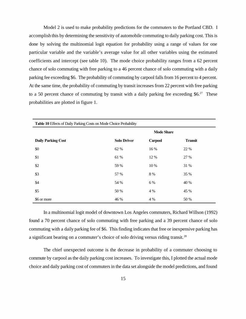
Model 2 is used to make probability predictions for the commuters to the Portland CBD. I

accomplish this by determining the sensitivity of automobile commuting to daily parking cost. This is

done by solving the multinomial logit equation for probability using a range of values for one

particular variable and the variable’s average value for all other variables using the estimated

coefficients and intercept (see table 10). The mode choice probability ranges from a 62 percent

chance of solo commuting with free parking to a 46 percent chance of solo commuting with a daily

parking fee exceeding $6. The probability of commuting by carpool falls from 16 percent to 4 percent.

At the same time, the probability of commuting by transit increases from 22 percent with free parking

to a 50 percent chance of commuting by transit with a daily parking fee exceeding $6.27 These

probabilities are plotted in figure 1.

Table 10 Effects of Daily Parking Costs on Mode Choice Probability

Mode Share

Daily Parking Cost Solo Driver Carpool Transit

$0 62 % 16 % 22 %

$1 61 % 12 % 27 %

$2 59 % 10 % 31 %

$3 57 % 8 % 35 %

$4 54 % 6 % 40 %

$5 50 % 4 % 45 %

$6 or more 46 % 4 % 50 %

In a multinomial logit model of downtown Los Angeles commuters, Richard Willson (1992)

found a 70 percent chance of solo commuting with free parking and a 39 percent chance of solo

commuting with a daily parking fee of $6. This finding indicates that free or inexpensive parking has

a significant bearing on a commuter’s choice of solo driving versus riding transit.28

The chief unexpected outcome is the decrease in probability of a commuter choosing to

commute by carpool as the daily parking cost increases. To investigate this, I plotted the actual mode

choice and daily parking cost of commuters in the data set alongside the model predictions, and found

16

Figure 1. Effect of Daily Parking Cost on Mode Choice Probability

0 %

1 0 %

2 0 %

3 0 %

4 0 %

5 0 %

6 0 %

7 0 %

8 0 %

$ 0 $ 1 $ 2 $ 3 $ 4 $ 5 $ 6

Daily Parking Cost

Mo

de

Ch

oic

e P

rob

abili

ty

D r i v e A l o n e

C a r p o o l

T r a n s i t

Figure 1. Effect of Daily Parking Cost on Mode Choice Probability

0 %

1 0 %

2 0 %

3 0 %

4 0 %

5 0 %

6 0 %

7 0 %

8 0 %

$ 0 $ 1 $ 2 $ 3 $ 4 $ 5 $ 6

Daily Parking Cost

Mo

de

Ch

oic

e P

rob

abili

ty

D r i v e A l o n e

C a r p o o l

T r a n s i t

that in this data set fewer commuters actually choose SOVs and carpools and more commuters choose

transit as daily parking cost increases. Therefore, the model’s counterintuitive mode choice results

for carpool commuters is explained by actual mode choice of commuters.

The model can also be used to predict the probability of employees commuting in SOVs based

on annual household income (see figure 2). I use the variable averages and the estimated coefficients

and intercept. The average price paid to park is $2 per day. The probability ranges from a 44 percent

chance of solo commuting with an annual household income of $5,000 to a 77 percent chance of solo

commuting with an annual household income exceeding $70,000. At the same time, the probability

of commuting by carpool falls from 9 percent to 6 percent. Commuters with an annual household

income of $5,000 have a 47 percent chance of commuting by transit, and commuters with an annual

household income exceeding $70,000 have a 16 percent chance of commuting by transit. Thus,

commuters in higher-income households have a more inelastic demand for driving when there is a

parking charge. The share of drivers who park free at work declines as their income increases. This

does not mean that lower-income commuters are more likely to be offered free parking at work.

17

Figure 2. Effect of Household Income on Mode Choice Probability

0 %

1 0 %

2 0 %

3 0 %

4 0 %

5 0 %

6 0 %

7 0 %

8 0 %

$ 5 , 0 0 0 $ 1 5 , 0 0 0 $ 2 5 , 0 0 0 $ 3 5 , 0 0 0 $ 4 5 , 0 0 0 $ 5 5 , 0 0 0 $ 6 5 , 0 0 0

Annual Household Income

Mo

de

Ch

oic

e P

rob

abili

ty

D r i v e A l o n e

C a r p o o l

T r a n s i t

Instead, lower-income commuters who are not offered free parking are more likely to ride the bus,

bicycle, or walk to work. Therefore, a greater share of lower-income drivers park free at work

because lower-income commuters are less likely to drive to work if they have to pay for parking. This

finding is useful in helping planners target certain demographic groups when they evaluate policies

and programs to reduce solo commuting.

The model can be used to predict the change in the number of vehicles used for commuting

(see table 11). With free parking, there would be 69 cars driven to the CBD (mode split is 62 percent

SOV, 16 percent carpool, 22 percent transit) for every 100 commuters and with a daily parking charge

of $6 there would be 48 cars driven to the CBD (mode split is 46 percent SOV, 4 percent carpool, 50

percent transit) for every 100 commuters. This relationship is shown graphically in figure 3. In other

words, the mode choice model predicts that a daily parking charge of $6 in the Portland CBD would

result in 21 fewer cars driven for every 100 commuters. This translates to a daily reduction of 147

VMT per 100 commuters and an annual reduction of 39,000 VMT per 100 commuters.29 I use the

change in the number of cars driven to work to estimate the price elasticity of demand for parking,

18

Figure 3. Effect of Daily Parking Cost on the Numberof Cars Driven by Commuters to the CBD

0

2 0

4 0

6 0

8 0

$ 0 $ 1 $ 2 $ 3 $ 4 $ 5 $ 6

Daily Parking Cost

Nu

mb

er o

f C

ars

per

100

C

om

mu

ters

which is shown in table 11.30 As expected, people’s demand for parking becomes more elastic as the

daily parking charge increases.

Table 11 Effect of Daily Parking Cost on Number of Cars Driven to the CBD

Daily parking cost

Number of Cars Number of cars per100 commuters

Price elasticity of demandfor parking at work

Solo driver Carpool Transit Total

$0 334 38 0 372 69 - 0.02

$1 329 28 0 357 66 - 0.07

$2 318 23 0 341 63 - 0.12

$3 307 19 0 326 60 - 0.18

$4 291 14 0 305 57 - 0.41

$5 270 9 0 279 52 - 0.44

$6 or more 248 9 0 257 48

Note: Based on the sample of 539 commuters in the mode choice model. The prediction for the number of cars driven bycarpoolers assumes a carpool occupancy rate of 2.3.

19

ConclusionUsing a household activity framework to evaluate mode choice is useful because detailed

information is collected about each activity/trip. Especially important for this study is the fact that the

Portland household activity survey collected information about the availability of free parking and the

price of paid parking at the destination for drivers and nondrivers.

Only the commute to work was examined in this study’s mode choice model. Because work

trips tend to be longer in distance than many other trip types (such as household provisioning,

recreational, social), commuters are less likely to substitute other modes for work trips. Commuters

are also more likely to pay to park their cars when commuting to work than traveling to other

destinations. For shorter trips, such as shopping trips, perhaps there is more opportunity for replacing

auto trips with walking and bicycling.

The multinomial logit model of commuter mode choice produces two key findings. (1) Parking

cost and the travel time by transit influence mode choice decisions for commuters. This suggests that

raising the cost of parking at work sites and decreasing the transit travel time (by iproving service and

decreasing headways) will reduce the percentage of people who drive alone to work. Of the non-

policy variables, income and vehicles per capita have an effect on mode choice, but whether the

commuter is male or female is unimportant. (2) Two land use variables are used in the mode choice

model. They are the proximity of the commuter’s residence to a light rail station, and the “pedestrian

connectivity” of the streets and sidewalks surrounding the commuter’s residence. Neither land use

variable has a significant effect on mode choice. This finding supports the contention that urban form

has little impact on mode choice decisions.

In study of travel and parking behavior, Mildner et al. (1998) found that cities with

interventionist parking policies, high parking prices and limited supply, frequent transit service, and

a high probability that travelers will pay to park are the most likely to have high transit ridership.

From a policy perspective, the provision of free parking by employers contradicts policies designed

to decrease solo driving and thus exacerbates the externalities associated with automobile use, such

as traffic congestion and poor air quality.31 The results of this study indicate that urban planners and

transportation analysts will have the greatest success in influencing the mode preference of individuals

(single occupant vehicle to carpool or transit) by charging commuters the true cost of parking or

20

allowing commuters to increase their income by “cashing-out” their parking spaces when they choose

to commute by another mode.32

21

SOURCES

Ben-Akiva, M. and S.R. Lerman. 1985. Discrete Choice Analysis: Theory and Application toTravel Demand. Cambridge, MA: MIT Press.

Boarnet, Marlon G. and Michael J. Greenwald. 2000. “Land Use, Urban Design and Non-WorkTravel: Reproducing for Portland, Oregon Empirical Tests From Other Areas.” Presented atthe 79t h Annual Meeting of the Transportation Research Board. January 9-13, 2000,Washington, D.C.

Cambridge Systematics. 1996. Data Collection in the Portland, Oregon Metropolitan Area.Oakland, CA: Cambridge Systematics.

Crane, Randall and Richard Crepeau. 1998. “Does Neighborhood Design Influence Travel? ABehavioral Analysis of Travel Diary and GIS Data.” Transportation Research, Part D. vol.3, no. 4, pp. 225-238.

Harvey, G.W. 1994. “Transportation Pricing and Travel Behavior.” Special Report No. 242:Curbing Gridlock: Peak-Period Fees to Relieve Traffic Congestion. vol. 2. Washington,D.C.: Transportation Research Board. pp. 89-114.

Horowitz, Joel. L. 1995. “Modeling Choices of Residential Location and Mode of Travel to Work.”In The Geography of Urban Transportation, 2nd ed. ed. Susan Hanson. New York, NY: TheGuilford Press.

MacKenzie, James J., Roger C. Dower, and Donald D.T. Chen. 1992. The Going Rate: What ItReally Costs to Drive. Washington, D.C.: World Resources Institute.

Mildner, Gerard C.S., James G. Strathman, and Martha J. Bianco. 1998. “Travel and ParkingBehavior in the United States.” Working Paper. Portland, OR: Center for Urban Studies,Portland State University.

NuStats International, Inc. 1995. “Oregon and Southwest Washington Household Activity and TravelSurveys.” Finale Report, 1995. Portland, OR: NuStats International.

Parsons Brinckerhoff Quade and Douglas, Inc. with Cambridge Systematics, Inc. and CalthorpeAssociates. 1993. Making the Land Use, Transportation, Air Quality Connection: ThePedestrian Environment: Volume 4A. Portland, OR: 1000 Friends of Oregon.

Schrank, D.L., S.M. Turner, and T.J. Lomax. 1990. “Estimates of Urban Roadway Congestion -1990.” Research Report 1131-5. College Station, TX: Texas A&M University, TexasTransportation Institute.

Shoup, Donald. 1994. Cashing Out Employer-Paid Parking: A Precedent for Congestion Pricing?in Curbing Gridlock: Peak-Period Fees to Relieve Traffic Congestion. vol. 2. Washington,D.C.: National Academy Press.

Shoup, Donald. 1995. “An Opportunity to Reduce Minimum Parking Requirements.” Journal of theAmerican Planning Association (Winter) pp. 14-28.

Shoup, Donald. 1997. “Evaluating the Effects of Cashing Out Employer-Paid Parking: Eight CaseStudies.” Transport Policy vol. 4. no. 4. pp. 201-216.

Shoup, Donald. 1999. An Invitation to Drive to Work Alone. Chapter of forthcoming manuscript.Los Angeles, CA: University of California, Los Angeles Institute of Transportation Studies.

Willson, Richard. 1992. “Estimating the Travel and Parking Demand Effects of Employer-PaidParking.” Regional Science and Urban Economics vol. 22, pp. 133-145.

Willson, Richard W. and Donald Shoup. 1990. “Parking Subsidies and Travel Choice: Assessingthe Evidence.” Transportation vol. 17, pp. 141-157.

Zupan, Jeffrey M. 1992. “Transportation Demand Management: A Cautious Look.” TransportationResearch Record 1346.

23

1.For discussion of the effect of employer-paid parking, see MacKenzie et al. (1992), Zupan (1992) and Willson and Shoup (1990).Willson and Shoup (1990) estimate that 90 percent of U.S. automobile commuters park free at work.

2.The activity survey included a stated-preference survey designed to analyze individual’s reactions to possible urban design and TravelDemand Management (TDM) actions such as congestion pricing and the availability and price of parking. Although stated-preferencemodeling has been used extensively in market research and in long-distance travel demand modeling, such techniques are now onlybeginning to be applied for urban area travel demand analyses.

3.Households were recruited by telephone; person, vehicle, and household information were collected by survey staff at this time.Recruited household were then sent a packet of information. Two days before their assigned travel days, households were sent areminder level. During the survey days, household members used activity recording sheets. (One reason for collecting two days’activity/travel data was to observe differences in travel behavior within households by day of week.) After the survey days, surveystaff collected activity information from respondents using CATI (computed-assisted telephone interviewing); 20,161 households werecontacted, and 4,451 household ultimately completed surveys.

4.Researchers use activity-based survey data to better understand the nature of the derived demand for travel. Travel is a deriveddemand because it is a means to an end, and the need to travel arises from the choice to conduct an activity out of the home.

5.Data was collected at the person, household, trip, and vehicle level, and all data files can be joined together using a unique samplenumber. The sample number can be located within a census tract or TAZ. In this way, several independent variables collected atdifferent levels of analysis (zone based vs. household vs. individual) can be joined together.

6.The estimate of total households is based on 1990 Census STF-3 data and factored to 1994.

7.The 1000 Friends of Oregon (1993) created a measure of pedestrian access, known as PEF (pedestrian environment factor).Pedestrian access is defined as a mixture of the ease of street crossings, sidewalk continuity, topography and whether a neighborhoodstreet network is primarily cul-de-sac or more open. Each category is scored on a scale from one to four (four being the bestranking), so each zone has a maximum possible score of 16 and a minimum of four. The higher the score, the more the zoneaccommodates non automobile travel. The study found that, as expected, residents in neighborhoods with higher density, proximityto employment, grid street pattern, sidewalk continuity, and ease of street crossing tend to make more pedestrian and transit trips,whereas residents of more distant, lower density suburban areas with auto-oriented land use patterns show extensive reliance on theautomobile.

8.A stratum was created for park-and-ride users by recording license plate numbers at park-and-ride lots. Names, addresses andtelephone numbers were obtained from the Department of Motor Vehicles, and the sampled households were recruited in the samemanner as household in other strata.

9.The survey firm is NuStats International, Inc.

10.It was not possible to recruit households without telephones for this survey, which may under represent low-income households.

11.The study is limited to work trip that end at a location within the Portland CBD. Since this is the site in the metropolitan area likelyto have the highest proportion of commuters who pay to park their cars, we are likely to see the effects of parking cost on commutermode choice. For this study, Portland’s CBD is designated as TAZs 1 through 16.

12.We can compare the mode choice distribution for Portland to national trends. Pisarski (1996) reports hat, excluding those whowork at home, the mode share for commuting in the U.S. in 1990 were solo driver (75 percent), carpool (14 percent), transit (5percent), and walk plus bicycle (4 percent).

13.Portland has, on average, 1.35 annual revenue hours of transit service per capita (Mildner et al. 1998).

EndNotes

24

14.Willson and Shoup (1990) present before-and-after data from five natural experiments in which employers who previously hadprovided free parking discontinue the practice. In four Los Angeles cases, they found that ending employer-paid parking reducedthe SOV mode share by 81 percent (Mid-Wilshire), 49 percent (Warner Center), 19 percent (Century City), and 44 percent (CivicCenter). Although I found a similar mode split in Portland as Willson and Shoup found in Los Angeles, Boarnet and Greenwald(2000) argue that travel diary data for Portland show higher frequencies of transit and walking trips than Southern California traveldiaries, suggesting that urban form features in Portland might more easily allow alternatives to driving.

15.Respondents to the household activity survey who used a mode other than a vehicle for the trip were asked “Would you have hadto pay to park if you went by car?”(Q11) [Yes/No] “How much would you have had to pay?” (Q11A) XX.X perHourly/Daily/Weekly/Monthly/Semesterly (Q11ATIME). Respondents who used a vehicle for the trip were asked “Did you payfor parking?” (Q24) [Yes/No] “How much did you pay for parking?” (Q25) XX.X per Hourly/Daily/Weekly/Monthly/Semesterly(Q25TIME). The prices reported were converted to a daily parking cost.

16.The annual congestion cost is $330 per traveler computed from Schrank et al. (1990). Eight transit accommodating cities in theU.S. have an average solo driver share of 68.4 percent.

17.It is important to mention up front that one possible source of error is the notion that there is a difference between the two groupsof commuters (those who pay to park and those who park free) that is not accounted for by the model specification.

18.This variable is likely to have survey respondent error. Transit riders were asked to report the price they would have paid topark if they drive, but they may not know this information accurately if they are non-drivers. Even drivers themselves may not knowexactly how much they pay for parking. For example, some commuters may have their parking fees automatically billed or deductedfrom their salary.

19.See Ben-Akiva and Lerman (1985) and Harvey (1994) for studies using logit models for predicting mode choice.

20.Parking cost and travel time by transit are the only cost variables included in the final models; other costs (fuel cost, automobilerunning cost, etc.) are excluded.

21.Travel times are calculated for TAZ-centroid to TAZ-centroid by the Portland Metro travel network analysis based on ME2modeling process. Inter and intrazonal A.M. peak period travel times on the highway and transit network were provided by PortlandMetro and generated by its travel demand model. The difference between auto and transit times allows the model to includecommuters’ sensitivity to longer travel times by transit versus automobile.

22.Land use variables are available from Portland Metro’s Regional Land Information System. This database is a set of GIS filescontaining information on census block groups, transportation analysis zones, streets and rail corridors.

23.Data are available on land uses at trip destinations as well as origins. However, all trips selected for the this study’s mode choicemodel end in the CBD, where the built and natural environment is conducive to pedestrian activity and transit access is good.Therefore, we concentrate on land use at the trip origin to determine its effect on mode choice.

24.It is often the case with transportation models that some of the factors that influence travel decisions are unobservable orunavailable, making it impossible to fully explain travel behavior.

25.Although the models perform well, the process of transforming discrete variables into dummy variables (having a value of 0 or 1)that are suitable for the logit model may introduce error into the procedure.

26.Managerial jobs tend to pay higher than non-managerial jobs, and this expands or constrains a commuter’s mode choice set.

27.The model predicts that with increasing daily parking cost there will be a greater shift among commuters from SOV to transit thanfrom SOV to carpool. There is a high up-front cost of forming carpools, and commuters may find carpools less convenient because

25

of reduced commuting flexibility and the lack of a car during the daytime for errands or emergencies.

28.Willson (1992) used data from a 1986 mode-choice survey of downtown office workers to estimate a multinomial logit model ofmode choice and parking demand. He found that eliminating free parking would reduce the SOV share from 72 to 41 percent,increase the carpool share from 13 to 28 percent, more than double the transit mode share 15 to 31 percent, and reduce the numberof cars that would be driven to work (cars used for SOV trips plus cars used by carpools) by 34 percent. The parking cost elasticityfor the same equation is -0.27 for the SOV mode, and the cross elasticity for transit is 0.35.

29.Assumes an average roundtrip commute distance of 7 miles.

30.The elasticity calculations use the arc elasticity formula.

31.This study’s inconclusive findings about the effect of land use on mode choice show that more research on the effect of urban formon travel behavior is needed before planners attempt to reduce congestion and air quality through changes in urban form. In addition,more research may be needed on the PEF land use strata developed by 1000 Friends of Oregon (1993) as an indicator of land use.

32.For a discussion of the costs and benefits of parking cash out, see Shoup (1994) and Shoup (1997).