The Effects of Geographical Indications andNatural Conditions on Wineyard Sale Prices

Jean-Sauveur Ay(a) and Julie Le Gallo(b)

September 8, 2013

Abstract

It is common knowledge that the taste of a wine depends on Natural Conditions (NCs)where grapes have grown, and that Geographical Indications (GIs), by grouping together similarNCs, also provide some information about the taste of a wine. Both GIs and NCs potentially addvalue to wineyards. However, disentangling their relative contributions is complex because oftheir spatial nesting. In this paper, we propose an estimation method that allows evaluating thesecontributions. This method takes into account some potential unobserved NCs and the resultingendogeneity of GIs in the hedonic equation. Using original data about wineyard sales fromBurgundy (France), we find, in accordance with previous studies, that GIs are a more importantsource of wineyard price variation than NCs. However, taking into account the possibility ofspatially omitted biophysical variables implies at least more than a doubling of the explainedpart from NCs (from 8% to 17%, where the GIs’ parts fall from 51% to 37%). Taking intoaccount the endogenity of GIs also sharply decreases their economic importance. From a naiveper-hectare premium of e 1.32 million for the most famous GIs (Grand Cru), the estimate ofour prefered model is about e 0.35 million, still highly significant nervertheless.

Keywords: Geographical indications ; wineyard prices ; endogeneity ; ordered modelsJ.E.L. Codes: C25, C26, C51, R33

(a): Corresponding author. CNRS, UMR 7204 CERSP F-75005 PARIS (principal affiliation) and INRA, UMR 1041CESAER F-21000 DIJON (associated researcher). jsay.site@gmail.com.(b): CRESE, Université de Franche Comté F-25000 BESANCON. jlegallo@univ-fcomte.fr.

Preliminary results, please do not quote. The authors acknowledge the data providers, which allowed this work tobe done. Wineyard prices are obtained from SCAFR – Terre d’Europe with the help of Jean Cavailhès and MohamedHilal (INRA Dijon). Spatial delineations of Geographical Indications come from the Institut National de l’Origine etde la Qualité (INAO) and we are grateful to Catherine Burrier (INAO) and Cécile Détang-Dessandre (INRA) to haveobtained the collaboration. Data about soil quality are obtained with the friendly help of Jean-Marc Brayer and PierreCurmi (AgroSup Dijon). Climate variables are obtained through the Observatoire du Développement Rural, we thankEric Cahuzac (INRA) and its colleagues for working on these variables and making them available.

1

1 Introduction

It is generally acknowledged that the taste of a wine depends on Natural Conditions (NCs) wheregrapes have grown and that consumers rarely taste a wine before purchasing. As a mean todifferentiate wines produced in similar NCs and to provide this simplified, objective informationto potential consumers, the relevance of Geographical Indications (GIs) is obvious. What is lessobvious is the relative contributions of these two nested characteristics – NCs and GIs – in the finalvalue of wines. This decomposition is nevertheless central because, in addition to the value addedfrom information availability (Akerlof 1970 ; Nelson 1970 ; Menapace and Moschini 2012), GIs arealso potential sources of undeserved rents for producers (Mussa and Rosen 1978 ; Besanko et al.,1987 ; Mérel and Sexton 2012). The economic outcomes of GIs are a combination of vertuousinformational content and surplus extraction by limiting supply and artificially segmenting winemarkets, making their recognition conflicting in trade negociations (Josling, 2006).

A large number of empirical papers is concerned with the determinants of wine value. Based ondata about wine prices, it appears that producer’s reputation (Combris et al. 1997 ; Ali and Nauges2007), technology (Gergaud and Ginsburgh, 2008) and expert’s opinion (Ali et al. 2008 ; Duboisand Nauges 2010) are important explanatory variables. However, uninformed consumers also usebottle price as a signal of quality, making the causal interpretation more delicate (Nerlove 1995 ;Costanigro et al. 2007 ; Schnabel and Storchmann 2010). Wine quality is also signaled throughGIs that are found to provide positive premiums (Ashenfelter et al. 1995 ; Combris et al. 2000 ;Carew and Florkowski 2010) increasing with wine prices (Costanigro et al., 2010). Even if they aremore scarce, some papers study the effects of NCs such as year to year climate variations (Lecocqand Visser 2006 ; Ashenfelter 2008) or land characteristics and exposure (Gergaud and Ginsburgh,2008). Analysing the effects of NCs on bottle prices is complicated by the necessity to matchprecisely the wines to the NCs where grapes grown. Consequently, the two closest papers to thisone (Ashenfelter and Storchmann 2010 ; Cross et al., 2011) prefer using wineyard sale prices toidentify the value of what we call NCs. The results of these two last papers are contrasted, usingrespectively data from the Mosel Valley (Germany) and the Willamette Valley (OR, United States).The first finds a strong effect of NCs through solar radiation index and the second does not find anysignificant effect, with or without controlling by GIs. Both find a positive effect of GIs on wineyardsale prices, up to $7,000 per-acre for Cross et al. (2011) (Table 2, p. 155).

Starting with a reduced equation from the hedonic theory applied to farmland (Palmquist, 1989),the present methodology semiparametrically estimates the effects of NCs through B-splines (Anglinand Gencay 1996 ; Bao and Wan 2004 ; Li and Racine 2007). It integrates potentially measurementerrors and omitted biophysical variables that describes NCs, a recurrent weakness of previous studies(Oczkowski, 2001). However, allowing for this possibility requires to model GIs as functions ofNCs in a first step. Although the exogeneity of biophysical variables is indisputable, GIs arespatially designated to picture similar (observed and unobserved) NCs, making them endogenous.In this context, our empirical strategy is twofold. (i) NCs are inherently a continous spatialsignal. Therefore, we argue that semiparametric Spatial Trend Surfaces (STSs) from geographicalcoordinates may act as proxies of the unobservable biophysical variables (Kammann and Wand2003 ; Fik et al. 2003 ; McMillen 2010). (ii) Spatially discontinous GIs are designated on the basisof historical considerations sometimes orthogonal to the NCs of wineyards (favoritism, personal

2

influences or false believes about biological mecanisms, according to Stanziani 2004 and Norman2010). Therefore, the endogeneity of GIs is controlled by using a more than two century oldadministrative subdivision (the communes) as multinomial instrumental variable. We evaluate theirappropriatness for the identification both through spatial error autocorrelation (Anselin 1988, usedas a test for misspecification by McMillen, 2003 and Le Gallo and Fingleton 2012) and throughsome adaptations of the IV post-regression tests to our particular case.

We apply our proposed methodology on a quasi-exhaustive database about wineyard sales1992–2008 in two wine regions within the French administrative region of Burgundy. These tworegions of wine production (Côte de Beaune, CDB, and Côte de Nuits, CDN) probably group themost expensive wineyards of the world, as they contain 37 wines in the 50 most expensive.1 Withinthese regions, GIs actually consist in a common hierarchy of wineyard plots (and resulting wines)according to a nationally wide scheme, the Appellations d’Origine Controlée (AOCs). First legallyestablished in 1855 for Burgundy under another scheme, these delineations initially come fromland classification schemes by the monks from Cîteaux around the Xth century (Stanziani 2004 ;Norman 2010). Actual GIs divide symetrically the two wine regions in Grands Crus (GCRUs),Premiers Crus (PCRUs), Villages (VILLs), Bourgognes Régionaux (BOURs) and Grands Ordinaires(BGORs), listed from the most famous to the less.2 These wineyards from Burgundy constitute awell-shaped application for at least three reasons:

1. GIs are delimited very finely (at the plot scale) and wineyard sale prices can be perfectlymatched with this information. Moreover, the presence of GIs’ names on the labels of winebottles is highly regulated through mandatory information and font sizes as examples.

2. CDB and CDN produce overwhelmingly terroir wines, implying a high homogenity in termsof both grape variety, technology and wine making process (Norman, 2010). Two grapevarieties represent more than 95% of the acreages (chardonnay and pinot noir).

3. Wine production and wineyard classification have a long history. This long-run temporalpredetermination of GIs provides some current variations of GIs orthogonal to NCs. Whatwas probably the result from lobbying two century ago is today arbitrary, hence exogenous.

The first point allows us to model GIs without errors-in-variables and to have high variationsof GIs at a fine scale, i.e., for locally similar NCs. The second point reinforces the use of thehedonic theory applied to farmland that substitutes the producers by the landowners as the agentfrom which the value is infered: Burgundy wine production presents less unobserved heterogeneitythan other potential French wine region. The third point allows us to identify the structural (causal)effect of GIs even if some NCs, correlated with GIs, are omitted from the regression functions.Contributions.

The outline of the paper is as follows. The section 2 presents the empirical issues relative to ourstudy: omitted variables, endogeneity of GIs’ designations. The data are presented in section 3. Theresults are reported in section 4. Finally, section 5 concludes.

1http://www.wine-searcher.com/most-expensive-wines (last accessed: September 8, 2013)2These five GIs are a grouping of the approximatively 800 official AOCs that the Burgundy counts, just for

its wines. This classification in five items (distinctively and systematically reported on the labels of wine bottles)provides an information about an objective quality, which is not the case for the numerous within AOCs. See http://www.vins-bourgogne.fr/gallery_files/site/12881/13118/18581.pdf (last accessed: September 8, 2013).

3

2 Empirical Issues

2.1 Separating GIs from NCs within an hedonic model

Because land is a non reproducible fixed asset, the Ricardian principle is that its price capitalizesthe comparative advantages provided to the final user. Therefore land price is a convenient andwell-used metric to recover the values associated to a large variety of spatialized attributes thatmatter economically (soil quality, legislative constrains, climate, ecosystem services, agriculturalsubsidies, see Ay and Latruffe 2013). Integrated within the hedonic framework, this moves thefocus of valuation from the output market to the landowners though the assumption of competitiveland markets. In our case, this helpfully allows to neglect the complex effects of producer’s wineportfolio, technology, reputation and ability, and the effects of consumer’s information, preferenceand habits to concentrate the modeling effort on the willingness-to-pay of potential landowners withthe highest bids.

By buying a wineyard plot i, a buyer acquires both the effects of NCs on grape quality andthe right to put the associated GIs on the wine that comes from this plot. Buyers and sellers areassumed to have a perfect information about both GIs and NCs, so the values of these attributes aretotally capitalized in the observed price per hectare pi. The econometrician only observes a partof the biophysical variables representing the NCs (Bi), and the vector of GIs noted Di. The otherbiophysical variables Wi are not observable but matter for observed land prices.

pi = α + βB>i + γW>i + δD>i + εi (1)

The row vectors β, γ and δ are the marginal prices and εi the residual with the usual properties.This is the classical hedonic framework, which, without loss of generality, we assume to be linear inparamaters for mathematical convenience. This equation admits non linear effects of variables, thegeneral hedonic case according to Ekeland et al. (2004). In order to simplify notations, we considerthe endogenous and the exogenous variables as nets of other price determinants that are neither GIsnor NCs: price inflation, buyer/seller characteristics or urban influence as examples. According tothe Frisch-Waugh-Lovell (FWL) theorem, it is always possible to orthogonalize the variables of aregression model and analyse their effects separatly (Davidson and MacKinnon, 2004).

Coupled with the zero conditional mean assumption E(εi | Bi, Di,Wi) = 0, equation (1)describes a structural relationship. Therefore, the Total Sum of Squares (SST ) of wineyard prices(their variance) can be decomposed in the sum of the Explained Sum of Squares (SSE) and theResidual Sum of Squares (SSR) according to the classical formula: SST = SSE + SSR. Theassumption of structural residuals involves a null covariance between the explanatory variables andthe residuals, ensuring a uniquely-defined additive decomposition between the explained and theunexplained part of price variations. The respective contributions of GIs and NCs are nested inSSE and are clearly indistinguishable at this point. Opening the black box of the explained partof price variations leads to an additive decomposition based on price’s conditional expectationsevaluated at the sample averages of the different variable sets.

SSE =∑

i

(pBi − p

)2+∑

i

(pDi − p

)2+∑

i

(pWi − p

)2+ 2 · Ω (2)

4

with pBi ≡ E(pi | Bi, D,W ) = α + βB>i + δD>

+ γW>

(3)

pDi ≡ E(pi | B,Di,W ) = α + βB>

+ δD>i + γW>

(4)

pWi ≡ E(pi | B,D,Wi) = α + βB>

+ δD>

+ γW>i (5)

and Ω = βδ · cov(Bi, Di) + βγ · cov(Bi,Wi) + δγ · cov(Di,Wi) (6)

The decomposition (2) is non unique but has the interest – relatively to alternative formulations,see Appendix XX – to treat symetrically both sets of variables. The interaction effect Ω is notstrictly allocable to a particular set of variables. It represents the loss of precision in the pricedecomposition due to correlations between wineyard attributes. It is interesting to note a parallelof this interaction effect with the problem of covariate imbalance in the treatment effect litterature(Rosenbaum and Rubin 1984 ; Imbens 2000). The respective contributions of each set of variablesare more precisely estimated when covariates are perfectly balanced, in which case Ω = 0.

If we are only interested in the joint effect of biophysical variables Bi ∪Wi (noted SSB) todescribe the effects of NCs, we can bind the SSE from B and W as well as the interaction betweenthese two subsets of variables.

SSB ≡∑

i

(pBi − p

)2+∑

i

(pWi − p

)2+∑

i

(pBi − p

)(pWi − p

)(7)

Only looking for SSB allows us to neglect the correlations between biophysical variables,letting our methodology free of assumptions about them. Nevertheless, the correlations with Di

stay of interest, as the direct part from the sum of squares of GIs which that are the same asin (2): SSD =

∑i

(pDi − p

)2. So, the decomposition of interest is about the uniquely definedSSE = SST − SSR and consists in indentifying the sum of SSB, SSD and two weightedcovariances – between (Bi, Di) and (Wi, Di) – that we note respectively ΩBD and ΩWD.

2.2 Omitted variable bias and proxy solution

By considering Wi as unobservable, this framework is sufficiently general to include the possibilitythat Bi contains error-in-variables,3 another usual problem in analysing the effects of biophysicalvariables on land prices. Therefore, the following “naive” estimation of the structural equation (1)would imply biased parameters (Wooldridge, 2002).

pi = αo + βoB>i + δoD>i + εoi (8)

In the (likely) case of positive correlations between Wi and both Bi and Di, the coefficientsβo and δo are upward biased as the estimated residuals. The effects of Wi are allocated betweenthe three last terms of the Right Hand Side of (8). In the resulting decomposition SST = SSBo +SSDo +SSRo + 2(Ωo

BD + ΩoWB), SSBo is downward biased relatively to SSB and the two others

sums of square are upward biased. Note that, contrary to SSBo and SSRo, the bias in SSDo onlycomes from the bias in the parameters βo and δo.

3Because the correlations betweenBi andWi are not constrained, one can consider the difference between measuredand true values of Bi as an additional column of Wi.

5

One solution to recover the structural decomposition consists in including a supplementaryterm (a proxy) in the regression function. Because of the strong spatial patterns displayed byobserved and unobserved biophysical variables (both from litterature and evidences from our data,see section 3), we use a Spatial Trend Surfaces (STSs) of geographical coordinates as this additionalterm. This approach – also called GeoAdditive modeling – allows to control some unobserved localeffects in the regressions (Kammann and Wand 2003 ; Fik et al. 2003 ; McMillen 2010). In ourcase, the STS ` substitutes with errors the effect of Wi.

γWi = `(xi, yi) + ηi (9)

The variables xi and yi represent respectively the longitude and the latitude of the plot i. Theterm ηi is a residual component, uncorrelated with the STS by construction. Because of the zeroconditional mean assumption on the structural model, we also know that these proxy residuals areuncorrelated with the structural main residuals εi. The resulting empirical model from the proxysolution induces a specific set of estimators indexed r.

pi = αr + βrB>i + δrD>i + `r(xi, yi) + εri (10)

It is generally acknowledged that the proxy variable solution provides a reliable estimation ofthe coefficients, but under strong assumptions. Wooldridge (2002, Chapter 4, pp. 63–64) providesthe sufficient conditions to trust a proxy variable solution, that we adapt to our case.

cov(xi, εi) = cov(yi, εi) = 0 (11)cov(xi, Bi) = cov(yi, Bi) = 0 (12)cov(xi, Di) = cov(yi, Di) = 0 (13)

The first condition (11) implies that the proxy variables do not have their own effect onthe outcome (i.e., independently from Wi). This is rarely controversial in classical approaches(according to Wooldridge, 2002) but can be problematic here as it is possible that location impactswineyard prices even if Wi is accounted for. Geographical coordinates have probably some propereffects: neighborhood effects, external economies, local land scarcity as exemples. For the pricedecompositions, the main implication of this condition is to know if the effects of `r(xi, yi) have tobe included in the SSBr or in the SSRr. If (11) is verified, the effects of the proxies clearly have tobe included in SSBr. If not, the effects have to be included according to their correlations with Bi

(observable) and Wi (unobservable). Under general settings, including the proxy effects in SSBr

(i.e., considering (11) as verified) provides a upper bound and including only the correlation withBi a lower bound of the true SSB. We compute both.

The second condition (12) is necessary for the good allocation of effects between the STS andthe observed biophysical variables. It is not fundamental here because both effects could be groupedin NCs if the condition (11) is verified: this condition is auxiliary to the first. However, to obtainreliable decomposition, we substitute a less usual condition which comes from the fact that theeffects of Wi are directly of interest here, contrary to the classical proxy framework which is mainlyconcerned on the coefficients of the true variables included in the model.

6

cov(εri ,Wi) = 0 (14)

This condition can be called “completeness” as it implies that not any effects of NCs are in theresiduals from the proxy specification. Even if less conventional, this assumption could be testedeasily in our case by knowing the amount of spatial autocorrelation in εri . As such, standard spatialautocorrelation test on residuals from the proxy model (Moran’s I for example, Anselin, 1988)allows us to evaluate the presence of omitted NCs in the proxy equation.

The last condition (13) is more complicated, as it drives the decomposition between our twomain effects of interest: GIs and NCs. Without it, GIs are endogenous in the proxy regression andcontrary to the failure of (11) we cannot estimate an interval of credible values for SSB and SSDwithout it. Relaxing this condition implies a non-trivial shift of the proxy solution that we adressin the following subsection. Just keep in mind that the proxy solution needs this condition to bereliable. Finally, a unbiased proxy estimation – conditions (11), (12), (13) verified – assures thatεri = εi + ηi. Consequently, SSRr overestimate SSR and, even if the parameters are without bias,a reliable estimation of SSB through SSBr can not be obtained without (14).

2.3 Endogeneity of GIs’ designations

2.3.1 History behind GIs and the two stage models

It is useful to divide GIs’ designation choices in two additive parts: one that is based on NCs andanother that is not. The first part is a function of both observed and unobserved NCs, observabilitystill being defined from the econometrician point of view. For the practionners and with experience,NCs are more precisely known and this knowledge is used in GIs’ designations. The second partcontains the deviations from this underlying NCs-based first part, in particular due to the previouslymentioned historical conditions. We assume that this second part is composed of a deterministicterm ψZ>i and a random one ξi. Because the GIs of interest have an ordinal structure (providing aquality classification of the resulting wines as in Ashenfelter and Storchmann 2010), we model thedesignation choices through a latent variable.

d∗i = θB>i + λW>i +ψZ>i + ξi (15)

This variable d∗i is the sum of the NCs-based part (the two first terms of the RHS), the “historical”part (the third term) and a residual (the last term). The first part does not represent truly what isusually called the potential of a wineyard in terms of wine quality, an appreciation that has to bedone on the wine market (by the consumers in particular). Even based on “objective” NCs, thispart represents the subjective quality potential in the minds of peoples that delineated the GIs,through the coefficients θ and λ. The matrix Zi typically contains historical conditions that haveinfluenced GIs’ designations: favoritism, personal influences or false believes about biologicalmecanisms. Because these latter variables are not observables, we use a more than two century oldadministrative subdivision that is known to be the local scale of political influence in French history.In Burgundy in particular, communes existed even before the 1789 French revolution and were thescale at which designation choices were made (Norman, 2010).

7

Intuitively, these deviations from NCs in GIs’ designations provide a mean to separate the effectsof GIs on wineyard prices from unobserved NCs. With (15) and λ 6= 0, the unobserved biophysicalvariables are clearly present in Di making (13) implausible. In effect, we have Di =

[d1i · · · dJi

]with J the number of GIs and with each component that comes from an indicator function.

dij = 1[µj−1 6 d∗i 6 µj

](16)

This structural form of GIs’ designation choices, (15) and (16), leads to an ordered qualitativemodel. The vector µ =

[µ0 · · ·µJ

]groups the thresholds of the latent variable to be estimated. By

convention, we put µ0 = −∞ and µJ = +∞. Coupling these two last equations with (1), we obtaina triangular system with an ordered structure of the J binary endogenous explanatory variableswhich first appears in Vella (1993). From a structural perspective, this does not imply importantchanges in the estimation process as the structural mean independence assumption stay verified(Lahiri and Schmidt 1978). However, when coupled with the fact that Wi is unobserved, the proxysolution is no longer usable due to the implausibility of (13). We can nevertheless write this firststep of GIs designations with the proxy solution.

d∗i = θrB>i + ψrZ>i + κr(xi, yi) + ξri (17)

This equation contain another STS, κr(xi, yi) ≡ λWi − ηi, which implies that ξri = ηi + ξi.This means that we can also evaluate the completeness condition (14) at this stage, through thespatial autocorrelation of ξri . But in all cases, the errors εri and ξri both contains ηi, so are correlated.We propose two solutions face to this problem for the reliability of both estimated coefficients anddecompositions.

2.3.2 Using Control Functions (CF)

Because ξri is contained in Di, our element of interest is now the correlation between the observedGIs and the unobserved biophysical variables that are not taken into account by the STS κr, thismeans cov(Di, ηi). The main implication of this endogeneity problem is that price variations fromGIs are overestimated in the proxy model. The Control Function (CF) approach assumes that theerrors εri and ξri are distributed according to a bivariate normal, using the result that the expectationof a marginal distribution conditionally to the another can be written analytically (Heckman 1979 ;Vella 1993 ; Newey et al. 1999).

E(ηi | d∗i ) = E(ξri | d∗i ) =∑

jdij ×

φ(µj−1 − d∗i )− φ(µj − d∗i )Φ(µj−1 − d∗i )− Φ(µj − d∗i )

(18)

Gourieroux et al. (1987) and Chesher and Irish (1987) call this term the generalized residuals,in a similar context than the previous latent variable framework with the assumption of gaussianresiduals. Controlling for endogeneity is then easily effectued by putting the conditional expectationas an additional covariate in what is now the second step of estimation.

pi = αc + βcB>i + δcD>i + `c(xi, yi) + ρc E(ξi | d∗i ) + εci (19)

8

The conditional expectation is estimated by a first step ordered probit model with the dummiescommunes as the instruments Zi. The coefficient ρc is the covariance between εi and ξi dividedby the variance of ξi. According to our omitted variable framework and to the fact that the twoerror terms are functions of ηi, we expect this coefficient to be positive. Decomposition of pricevariations with control functions: to be done.

2.3.3 Using Instrumental Variables (IV)

We also suggest to estimate the structural parameters in equation (1) by controlling omitted variablebias and endogeneity of GIs’ designations by using an Instrumental Variable (IV) approach, thatdoes not necessitate the normal assumptions basing the CF approach. An instrument should besufficiently correlated with the endogenous variable and uncorrelated with the error terms of (1). Inour setting, recall that the system of equations (1), (15) and (16) is triangular, where the estimationof (15) and (16) can be considered as the first sep of a Two Stage Least Squares (2SLS) approachto IV. In (15), variables contained in the matrix Zi play the role of instruments, i.e., the variablesthat verify the exclusion condition. For the reasons that are detailed above, these instruments arethe communes dummies. Because they were constituted 200 years ago, they do not affect directlythe price of a bottle and hence can be considered as valid instruments. However, several problemsarise in order to implement IV/2SLS in our particular setting. One possibility would be to usedirectly a standard IV estimator on (1). In other words, (1) is estimated using IV with all exogenousbiophysical variables and the set of communes in our sample as instruments for the dummies Di.However, proceeding in this way implies that we overlook that the ordered nature of the dummiesDi that appear in (1) so that there relative effects might not be estimated correctly.

Alternatively, we can use a 2SLS approach: the estimated d∗i from (15) with an orderedqualitative estimator are directly plugged into (10). However, this method correspond to forbiddenregressions (Angrist and Pischke 2008, p. 191–192) as the first stage is nonlinear. To overcomethis problem, we propose to adapt the procedure described in Angrist and Pischke (2008) forone endogenous dummy variable. This means running an intermediate linear probability step byregressing the dummies Di on all the exogenous variables (including the STS) and the predictionsof the latent variable from the ordered qualitative models as an instrument: Di = αl + βlB>i +

`l(xi, yi) + τ ld∗i + εli. The statistical significance of the coefficient τ ` can be used to estimatethe relevance of the instruments in explaining the endogenous covariates. Finally, we plug thepredictions from this intermediate step Di in the structural equation.

pi = αv + βvB>i + `v(xi, yi) + δvD>i + εvi (20)

This procedure allows using conventional IV in our particular case of J endogenous dummyvariables corresponding to an ordered qualitative variable. However, its main drawback is that isuses the nonlinearity of the first stage as an additional source of identifying information. In orderto control this potential caveat, we estimate (15) using different nonlinear estimators for ordereddependent variables.

Decomposition of price variations in IV: to be done. nonparametric IV models (Das, 2005)

9

3 Data

3.1 Sample

Our proposed methodology is applied to the most famous wineyards of Burgundy, which is a Frenchregion. Burgundy is geographically cut in two main spatial delineations of interest. The first isan already mentioned administrative delineation that exists at the national scale: the communes,which are kind of municipalities. The second describes spatial units known as homogenous in termsof geology and soils, according to a regional soil survey (Référentiel Pédologique de Bourgogne,Chrétien, 2000). This survey is effectued by soil scientists, independently from the current research.The left panel of Figure 1 colors the four wine regions of Burgundy, from which we keep only Côtesde Beaune (CDB) and Côtes de Nuits (CDN). Both Hautes Côtes de Beaune and Hautes Côtesde Nuits are other wine regions that have their own GIs and do not share the same structure thanCDB and CDN in terms of Villages (VILLs), Premiers Crus (PCRUs) and Grands Crus (GCRUs).Morever, GIs from Hautes Côtes are younger and spatially segregated from the other, that makethem hardly comparable with the CDB and CDN.

Beaune

Brochon

Chambolle−Musigny

Chassagne−Montrachet

Fixin

Flagey−Echézeaux

Gevrey−Chambertin

Meursault

Morey−Saint−Denis

Nuits−Saint−Georges

Pernand−Vergelesses

Pommard

Puligny−Montrachet

Santenay

Ladoix−Serrigny

Volnay

Côte de BeauneCôte de NuitsHaute Côte de BeauneHaute Côte de Nuits

5 km

NORTH

Vineyard Sale

8

8

8

9

9

9

9

10

10

10

10

10

10

10

11

11

11

11

11

11

11

11

12

12

12

12 12

12

12

13

13

13

13

13

Expl. Variance= 0.573

Figure 1: Wine regions and communes (left panel), soil units and wineyard sales (middle panel),spatial smoothing of the logarithm of sale prices (in deflated euro/ha, right panel)

The left panel shows the delineation of the communes (superimposed with the delination of wineregions) from which only the names of communes with well balanced GIs appear (see Appendix A.1for the details). Northern regions have principally the pinot noir as a wine variety to make red winesand southern regions have principally chardonnay to make white wines. Some exceptions exist,maybe the more typical are the communes of Pommard and Volnay which mainly produce red winesalthough being in CDB. The delination of soil units is more biophysically oriented, so the spatialpolygons are much more irregular. The middle panel of Figure 1 shows that only few soil unitsconcentrate the essential of wineyard sales. The presence of wine production (and, consequently,wineyard sales) is strongly explained by the geological and soil attributes and sales are principallylocated at the middle of each commune on the East–West gradient. The right panel of Figure 1displays the spatial distribution of the logarithm of per-ha prices, globally between exp(8) ≈ 3, 000

10

and exp(14) ≈ 1, 200, 000 in deflated e 2008. The two wine regions are comparable in averageprices and present a core(s)/ periphery structure. CDB (at the South) presents four cores, located atthe center from the East–West gradient and regularly along the South–North gradient. CDN (at theNorth) displays only one core, at the middle of the South–North gradient but shifted at the West.

3.2 Variables

The variables of our final database come from five main sources. The first concerns wineyardsales from the Société Centrale d’Aménagement du Foncier Rural (SCAFR), the French regulatoryinstitution of the farmland market. This database normally contains all land sales operated between1992 and 2008, for which the productive orientation (nature cadastrale) is wineyard. This databasecontains principally the observed price for each sale, the acreages, the identifiants of plots and somequalitative information: date of the sale, socio-demographics of seller and buyer, land tenure andthe presence/absence of building. The second database from the Institut National de l’Origine etde la Qualité (INAO) reports the spatial delineations of GIs, which allow to know exactly the GIof each parcel of each sale. The third set of variable comes from a Digital Elevation Model thatcomputes for each plot the elevation, slope and exposition. Because the resolution of this DEMis 50 meters, we can consider these biophysical variables as perfectly observed. This is not thecase for climate and soil quality variables that come from the two last databases at more aggregatedscales: respectively the communes and the soil units.

Table 1: Frequencies and proportions of wineyard sales for each GIs within each wine region

BGOR BOUR VILL PCRU GCRU Sum

CDB 177 463 924 393 32 1989(%) (5.49) (14.36) (28.65) (12.19) (0.99) (61.68)

CDN 124 207 739 126 40 1236(%) (3.84) (6.42) (22.91) (3.91) (1.24) (38.32)

Sum 301 670 1663 519 72 3225(%) (9.33) (20.78) (51.56) (16.10) (2.23) (100.00)

With a pooled sample of 3,225 wineyard plots sold, CDB and CDN contain respectively 1,989(61.7%) and 1,236 (38.3%) observations. The frequencies of GIs are rather similar within wineregions: the GI Village (VILL) represents the highest number of sales for both regions, followedby Bourgogne (BOUR), Premier Cru (PCRU), Grand Ordinaire (BGOR) and finally Grand Cru(GCRU). From the left to the right of the table, GIs are ordered from the less famous to themost. Sales frequencies are not monotonically related to reputation, the highest numbers of salescorrespond to the intermediate GIs.

Our sample of 2,978 wineyard plots represents 1,476 sales. Note that 907 sales are about onlyone plot and the sale with the highest number of parcels counts 73 parcels. All wineyard plots in onesale have the same reported par-hectare price. From Figure 2, the natural logarithm of per-ha pricesis more variable between GIs than between wine regions. This result both implies that there exists

11

LOGARITHM OF PRICE (DEFLATED EUROS/ HA)

WIN

E R

EG

ION

CDB

CDN

8 10 12 14

: AOC BGOR

CDB

CDN

: AOC BOUR

CDB

CDN

: AOC VILL

CDB

CDN

: AOC PCRU

CDB

CDN

: AOC GCRU

Figure 2: Within wine regions price distributions for each Geographical Indication, from the lessfamous (bottom) to the most (top)

strong variations of vineyard prices at small scales (within wine regions) and that GIs’ effects haveglobally the same magnitudes (between wine regions). Moreover, the medians are approximativelylinear from the BGOR of CDB to the GCRU of CDN, from the bottom to the top of Figure 2. Thismeans that the median price of one ha of GCRU is approximatively two times higher that onehectare (ha) of PCRU, itself two times more expensive than a VILL and so on. This Figure alsoshows the presence of some potential outliers in terms of price per-hectare, conditionally to the GIs.We report the econometric results with the outliers but we verify systematically that the results arenot too sensitive to their presence.

3.3 Summary statistics

The following Table 2 reports the usual summary statistics for continous variables contained in thefinal samples. Wineyard plots from Burgundy are very small (compared with other agricultural landuses and other wine regions in France). Average acreages correspond respectively to about .56 and.46 acres respectively for the CDB and CDN. The acreages are more variables for the CDB with aStandard Deviation near than three times higher.

The spatial coordinates (centered and reduced from the pooled sample) clearly show the spatialposition of the two wine regions that appears at the left panel of Figure 1. If we cut the whole regionin four regular rectangles, CDB is at the southern west (low longitudes and latitudes) and CDN is atthe northern east (high longitudes and latitudes). We compute the distances from wineyards to thecenters of communes, which group in general the service available to the population. This variableis used as a proxy of urban influence. The two wine regions share the same proximity of their

12

Table 2: Summary statistics for continous variables, separated sample for each wine region

Côte de Beaune (N= 1,846) Côte de Nuits (N= 1,132)Variables Mean St. Dev. Min Max Mean St. Dev. Min Max

Price (1,000 euro/ha) 252.83 296.10 1.27 3, 929.03 247.07 262.00 2.34 1, 822.79Surface (ha) 0.22 0.41 0.001 13.37 0.14 0.14 0.001 1.14Longitude (scaled) −0.70 0.51 −1.92 0.48 1.15 0.19 0.47 1.50Latitude (scaled) −0.70 0.42 −1.54 0.13 1.15 0.44 0.06 2.01Distance to Center (km) 1.19 0.57 0.08 3.67 1.00 0.51 0.07 2.90Elevation (100 m) 2.66 0.48 2.12 4.76 2.69 0.26 2.17 3.79Slope (degree) 4.67 4.81 0.00 23.61 3.14 3.37 0.40 19.65Temperature (Celsus) 11.16 0.26 10.92 11.49 11.10 0.18 10.92 11.515Precipitations (mm) 809.94 17.76 789.37 842.16 816.27 27.01 749.96 841.33Solar Radiation (Joules) 984.93 17.86 952.00 1, 000.52 972.09 16.00 953.08 1, 003.61Humidity (mm) 940.57 5.47 931.05 944.90 936.71 3.64 930.73 943.98Wind (km) 30.25 2.48 27.31 33.41 30.48 2.25 28.90 35.69Snow (cm) 26.14 7.10 17.05 39.95 31.25 6.04 22.39 39.34Water Holding Capacity (mm) 91.08 36.91 0 153 73.32 40.51 0 188Soil Depth (cm) 52.96 19.61 0 93 47.96 19.74 0 80Stone Rate (permil) 13.55 14.76 0 50 23.71 16.28 0 85Silt Rate (percent) 49.93 7.41 0 60 46.21 12.28 0 66Sand Rate (percent) 15.04 6.43 0 33 15.41 5.59 0 40Clay Rate (percent) 34.70 4.63 0 55 35.98 9.31 0 45

vineyards to these centers. The within distributions of all biophysical variables are rather similarbetween the two wine regions. Nevretheless, we can note that elevation appears as more variablefor the CDB and that slope is higher on average. Despite a North–South difference in locations,average temperatures do not really differ between the regions. Aggregate variables (the 12 last rows)present smaller coefficients of variations that the others perfectly observed variables. It is particulartrue for climate variables compared with elevation and slope.

In a unreported analysis, we find high correlations between the numerous biophysical variablesthat are relevant to explain both GIs’ designation and wineyard prices. Hence, we operate twoPrincipal Component Analysis (PCA) to reduce the dimension of the covariates and to decreaseproblems of multicolinearity in the econometric models. Correlated covariate are separated betweenclimate (rows 8–14) and soil (rows 15–20) variables that are plugged in two PCAs. We keep thetwo principal axis of both. Each of them explains respectively 87 and 72 percents of the empiricalvariances of the initial variables (see Appendix A.1 for the details).

13

4 Results

4.1 Naive and proxy hedonic models

4.1.1 Marginal significance of variables

We first report the results from naive hedonic models that ignore the possibility of omitted biophysi-cal variables and the endogeneity of GIs’ designations. To take into account the strong nonlinearitiesin the effects of biophysical variables on prices, we use both semiparametric B-Splines4 and poly-nomial terms. The splines fit better the data in general but the results are less easily interpretable.As it is more usual to use polynomial terms in econometrics, we provide the results from the twomethods. We estimate six specifications for each of the three samples (pooled, CDB and CDN),the spline orders are chosen according to a forward selection and the polynomials are limited tothe second order to keep the interpretations simple. The first two specifications only contain thevariables about NCs, only observed biophysical variables for (I) and with STS of geographicalcoordinates for (II). The specifications (III) and (IV) only contain the GIs’ dummies, respectivelywith and without STS. The two last specifications (V) and (VI) include both GIs and NCs, with andwithout STS. The results obtained from splines models are reported in the following Table 3. Thedetails of the coefficients from polynomials models are reported in Table 10 of the Appendix A.3.

In Table 3, the values reported are the increases in terms of SSE that follow the introduction ofall the spline terms of each variable, indicating the marginal significances for each of them (Foxand Weisberg, 2010). These numbers are close to the usual Fisher statistics for the joint nullity ofthe spline coefficients associated to each variable (the “order” columns also represent the degreesof freedom). Knowing that SST is 2,636 for the pooled sample, the R-squared can be computedfrom the last row of the top panel: R2 = 1 − SSR/SST . They are respectively .31, .53, .52,.65, .60 and .67 for the specification (I)–(VI). The SST for the CDB and the CDN samples arerespectively 1,766 and 871, so the R-squared ranges are .40–.67 and .47–.75 for all the specifications.For specifications (I), elevation appears as the most important biophysical variable, even if forthe CDN sample WET is equally strong. The effects of slope is strong for the pooled sample butnot for the others. Looking at the specification (II), the inclusion of STS sharply decreases thecoefficients associated to biophysical variables and increase the R-squared. STS are individuallyhighly significants such that specifications (II) fit the data better than specifications (III) that includeonly GIs. However, GIs have strong effects too where included alone in (III). For the three samples,the SSE just stemming from GIs are close to the SSR which means that the partial R-squaredfor the all four dummies is about 1/2. Including STS simultaneously with GIs – specification(IV) – implies a division by two of the marginal effects of GIs. This results still holds for thespecifications with both biophysical variables and GIs: between (V) and (VI). By comparing theindividual significances of biophysical variables (elevation in particular) between (I) and (V), we seethat including GIs strongly decrease their effects. The reverse is also true, albeit at a lesser extendwhen we include observed biophysical variables in addition to GIs: by comparing specifications(III) and (V). The same evidences are found on the more classical polynomial regressions of order

4http://cran.r-project.org/web/packages/crs/vignettes/spline_primer.pdf (last accessed: Septem-ber 8, 2013).

14

Tabl

e3:

Mar

gina

lExp

lain

edSu

ms

ofSq

uare

sfo

reac

hva

riab

les

and

sam

ples

,mod

els

with

splin

es

Pool

edSa

mpl

eV

aria

ble

Ord

er(I

)(I

I)(I

II)

(IV

)(V

)(V

I)

YE

AR

16.

978.

7412

.76

7.53

5.51

7.21

GIs

412

72.0

752

6.46

741.

1337

9.81

DE

PTH

35.

600.

246.

991.

69E

LE

V.4

228.

587.

0017

.77

4.87

HE

AT

323

.14

21.1

537

.17

13.8

8SL

OPE

310

2.91

14.1

98.

803.

76R

OU

GH

336

.39

20.4

710

.99

0.37

WE

T3

94.3

224

.04

52.5

84.

12X

514

6.83

93.2

934

.79

XYa

X34

0.44

152.

8797

.35

Y5

148.

6612

0.95

41.6

0E

XPO

.3

28.3

319

.86

1.84

0.83

DIS

T.3

29.4

336

.36

11.9

915

.80

13.0

618

.21

Res

idua

ls1

1806

.82

1248

.48

1257

.35

912.

7010

65.6

986

8.67

Cot

ede

Bea

une

Cot

ede

Nui

tsV

aria

ble

Ord

er(I

)(I

I)(I

II)

(IV

)(V

)(V

I)(I

)(I

I)(I

II)

(IV

)(V

)(V

I)

YE

AR

12.

124.

1814

.38

5.37

5.06

4.82

9.37

7.98

3.25

2.80

3.08

2.43

GIs

483

6.05

303.

5740

3.47

245.

5744

3.82

108.

1918

9.21

85.3

9D

EPT

H3

16.3

23.

797.

153.

291.

310.

823.

520.

56E

LE

V.4

204.

954.

788.

403.

317.

791.

481.

952.

95H

EA

T3

36.8

68.

0639

.79

3.80

52.0

31.

9033

.98

1.02

SLO

PE3

17.9

15.

884.

291.

388.

152.

204.

424.

81R

OU

GH

339

.22

8.06

22.1

52.

6052

.35

8.84

5.50

1.17

WE

T3

85.7

139

.72

73.7

625

.61

58.2

015

.32

32.6

16.

27X

563

.09

72.4

422

.45

46.7

820

.85

11.4

7X

Ya

X18

2.20

94.9

854

.69

57.3

840

.63

31.8

5Y

548

.60

57.9

222

.84

25.0

068

.34

10.6

2E

XPO

.3

33.6

628

.35

0.51

0.50

7.82

3.10

5.72

2.48

DIS

T.3

26.3

720

.78

17.1

615

.1A

13.0

912

.32

9.59

0.94

0.05

0.43

1.41

0.07

Res

idua

ls1

1067

.62

830.

1484

5.52

625.

6866

4.16

584.

5846

3.41

303.

5239

4.32

236.

8827

4.20

218.

12

Not

es:(a)

The

XY

row

sar

efo

rthe

inte

ract

ion

betw

een

the

splin

esof

each

geog

raph

ical

coor

dina

te,t

oin

crea

seth

efle

xibi

lity

ofST

S

15

two, reported in Table 10 of the Appendix A.3.

4.1.2 Marginal effects

The marginal significances of GIs as a whole are highly variable according to the different spec-ifications (with and without biophysical variables and with and without STS) but some featuresremain relatively robust between samples. Because the effects of GIs are modeled through dummiesvariables, the following Table 4 reports the marginal effects of GIs’ dummies5 and the standarderrors estimated by the delta method. For spline functions, the marginal effects are displayed byplotting conditional predictions with all other variables at their samples means (Fox and Hong,2009). These effect plots are reported in Figure 6, Appendix A.2 for each of the three samples.

Table 4: GIs’ marginal effects and standard errors from spline models, GI ref.: Grand Ordinaire

Bourgogne Village Premier Cru Grand Crueffect s.e. effect s.e. effect s.e. effect s.e.

POOL (III) 92.80 24.00 722.60 100.30 1441.80 197.90 4310.00 695.60POOL (IV) 54.90 21.70 605.30 104.90 829.70 157.20 3030.70 591.20POOL (V) 68.30 21.90 685.80 101.10 1273.10 198.20 4747.70 817.10POOL (VI) 48.50 21.60 526.90 94.90 726.10 141.20 2535.80 517.80

CDB (III) 120.50 38.20 881.30 167.10 1595.60 297.10 4083.50 1124.30CDB (IV) 87.30 34.60 772.70 481.70 1049.80 1238.10 3496.40 3256.00CDB (V) 77.40 32.50 810.60 164.90 1137.00 244.70 4447.80 1317.70CDB (VI) 102.30 57.10 813.20 1079.50 1103.20 4784.40 3565.10 8959.00

CDN (III) 64.20 29.30 579.80 117.90 1496.30 303.20 3955.10 769.70CDN (IV) 14.80 40.40 355.70 196.50 510.30 286.90 1234.30 748.00CDN (V) 58.60 33.70 605.00 170.30 1088.40 321.10 3030.10 798.30CDN (VI) 29.10 35.10 365.40 153.20 543.50 241.30 1347.20 573.60

The marginal effects of GIs on wineyard prices are high. Relatively to the GI Grand Ordinaire,a wineyard designated Bourgogne is 92.8% (σ = 24) more expensive according to specification (III)on the pooled sample. This number falls to 48.5% (σ = 21.6) when omitted biophysical variablesare taken into account through the proxy STS solution. When evaluated at the average price of aGrand Ordinaire wineyard (e 51,968), these premiums correspond respectively to e 48,227 ande 25,205. Recall that Cross et al. (2011) found $7,000 for the biggest premium in Oregon. Forthe more famous GIs, the premiums are incommensurate: respectively e 273,823, e 377,345 ande 1,317,825 for Village, Premier Cru and Grand Cru according to the conservative specification(VI) on the pooled sample. These magnitudes are similar within each wine regions CDB and CDN,even if certain differences appear. For such high numbers, the associated uncertainty is high as thestandard errors are quite important but the premiums are often significant two-by-two, i.e., betweenadjacent GIs on the reputation scale. Including STS implies an important decrease of the premiumsof the Premier Cru, in particular relatively to the premiums of Village (it is clear for the pooled

5We use semi-log models, the marginal effects of dummies are 100× [exp(δ − σδ/2)− 1], see Kennedy (1981).

16

sample between specifications (III) and (IV), and (V) and (VI) but also for the others samples).Note that the specifications with STS on the CDB sample – (IV) and (VI) – present high standarderrors for the effects of famous the GIs (Village, Premier Cru and Grand Cru).

From Figure 6 of the Appendix A.2 displays the marginal effects of elevation and slope forthe pooled sample, the CDB and CDN. They are reported with and without controlling for GIs,specifications (I) and (V). Between the two specifications, the magnitudes of the effects of thisbiophysical variables decrease: the curves are more flattened in (V). In general, the effects ofelevation are shapped as an inverted U and the effects of slope are concave. For the pooled sample,the elevation with the higher wine prices is of about 240m, For the CDB and the CDN the values areabout 280 and 260. The slope effects are highly increasing at low values and become non significantfrom 10 degrees. Globally the effects from the pooled sample are closest to those from CDB, whichcan be understood by the higher number of observations. The hedonic marginal prices of thesebiophysical attributes are the derivative of the effect curves. Elevation and slope have positive ornegative values, depending at the level of evaluation.

4.1.3 Spatial autocorrelation

As we argue in subsection 2.1, one way to evaluate the relevance of the proxy solution (equation 14)is to test for spatial autocorrelation of the errors from the hedonic equation. The following Figure 3displays the Moran’s plots for the specifications (I)–(VI) on the pooled sample, for the North-Westto the South-East. These plots present on the x-axis the estimated errors for each sale i and onthe y-axis the average errors of these neighbors, weighted according to their distances to i. Thespatial weight matrix is a gaussian spatial kernel with a bandwith chosen in order to have at leastone neighbor for each observation.

Figure 3: Moran plots for spatial autocorrelation of residuals, pooled sample

var

Moran's I= 14.001

var

wx

<−

lag.

listw

(spw

, var

)

Moran's I= 22.171

var

wx

<−

lag.

listw

(spw

, var

)

Moran's I= 8.869

Moran's I= −0.113

wx

<−

lag.

listw

(spw

, var

)

Moran's I= 0.636

wx

<−

lag.

listw

(spw

, var

)

Moran's I= −0.543

WIT

HO

UT

SS

FW

ITH

SS

F

NCs GIs NCs + GIs

This Figure clearly shows the interest of STS to control for the spatial autocorrelation of theresiduals, and this is true for each specification. Not any spatial effect stay in the residuals aftercontrolling by STS. This involves that the proxy STS solution is sufficient to take into account anyomitted spatial biophysical variable. More formally, a bootstrap inference of the Moran’s I statistics

17

indicate that we reject the spatial independance of errors for the models without STS but we cannotreject it for the models with STS (95% for (II) and (VI), 90% for (IV)). To investigate deeper thespatial structure of the residuals and the proposed solution throught STS, the following Figure 4displays three STS estimated on the residuals from the specifications (I), (III) and (V) at the top andthe three estimated STS r(xi, yi) for the specifications (II), (IV) and (VI) at the bottom.

Figure 4: Maps of estimated residuals from models without STS – (I), (III) and (V), top panel – andthe estimated STSs when there are in models: (II), (IV) and (VI), bottom panel

−2

−2

−1.5

−1.

5

−1

−1

−1

−1

−1

−1

−0.

5

−0.

5

−0.

5

−0.5

0

0

0

0

0

0

0

0.5

0.5

0.5

0.5

1

1

−1.

2

−1.2

−1.2

−1

−1

−0.6

−0.

4

−0.4 −

0.4

−0.4

−0.2

−0.2

−0.

2

−0.2

−0.

2 0

0

0

0

0

0

0

0

0.2

0.4

−0.8

−0.6

−0.4

−0.

4

−0.4

−0.2

−0.

2

−0.2

−0.2

−0.

2 −

0.2

−0.2

0

0

0

0

0

0

0

0.2

0.2

0.4

10

10.

5

10.

5

11

11

11

11.

5

12

12 12 1

2

12

13

13

13

13

13

13.5

13.

5

14

14

14

14

14.

5

15

11

11

11

11

11

11

11.

5

11.

5

11.

5

11.

5

11.5

12

12

12

12

12

12

12.

5

12.5

12.

5

11

11.

5

12

12 12

12

12

12

12

12.

5

12.5 1

2.5

12.5

13

13

13

13

13.

5

13.

5

RE

SID

UA

LSS

MO

OT

HE

D F

UN

CT

ION

S

(I) and (II) (III) and (IV) (V) and (VI)

Residuals on the three map at the top look closely to the spatial distribution of price as it appearsin Figure 1 but some differences exist in details. Errors are more important in the CDN for thespecification (I) with only NCs and the errors are more important in the CDB in the specification(III) with only GIs. In specification (V) the errors are equally variable between the two wine regions.The three STS at the bottom globally displays the same spatial patterns, even if some differencesalso appears in details. The STS are less marked from the left to the right, according to what Table 3presents. CDN presents a high East-West gradient in the specification (II), which decreases (butstays) in the specifications (IV) and (VI).

18

4.1.4 Decompositions

If we turn to the wineyard price decompositions between the GIs (SSD) and the NCs (SSB) forthe specifications (V) and (VI) that contain both GIs and NCs, contrasting evidences appear. Theyare summarized in the following Table 5. For both specifications, GIs appear as a more importantsource of wineyard price variation than NCs. However, taking into account the possibility ofspatially omitted biophysical variables for the pooled sample implies more than a doubling of theexplained part from NCs, from 7.62% to 16.56% between (V) and (VI). The naive hedonic model(and, therefore, previous analysis from other papers) underestimates the share of price variationsthat comes from NCs and overestimate the variations from GIs. Both with and without taking intoaccount the possibility of omitted biophysical variables, CDB has smaller proportions of explainedvariations due to NCs than CDN, an interesting result to describe the differences between the twowine regions. It is also interesting to note that the interaction effects are increasing when adding aSTS to the regression functions. Hence, controlling for omitted variables is done at the cost of aloss of precision in the decompositions.

Table 5: Decompositions of price variations according to naive models (V) and proxy solution (VI)

Sample Spec. SSB SSD SSR Ω

POOL (V) 7.62 50.97 40.42 0.99POOL (VI) 16.56 37.63 32.95 12.86CDB (V) 11.20 47.08 37.61 4.11CDB (VI) 15.75 42.20 33.11 8.94CDN (V) 15.07 49.14 31.50 4.29CDN (VI) 24.33 31.51 25.06 19.10

4.2 Ordered models of GIs’ designations

In this section, we report the results from the first step of ordered qualitative models on GIs’designations. Because these models of designation have an interest of they own, we estimatefour specifications both with logistic and probit errors for a total of eight estimations. All thespecifications contain the perfectly observed biophysical variables (elevation, slope and exposition),what distinguishes the four specifications is the following:

• (i) : only commune and soil unit dummy variables in addition

• (ii) : only climate and soil biophysical variables in addition

• (iii) : (i) with STS

• (iv) : (ii) with STS

We cannot include simultaneously the biophysical variables and the dummies because of perfectcolinearity (recall that continous biohysical variables come from aggregate sources at the commune

19

and soil units scales) so these specifications are complementary. Because the communes dummiesare our instruments, we only use the specifications (i) and (iii) with the probit errors as the firststep in our CF and IV approaches. The other estimations are displayed to show that the processesunderlying GI’s designations are closely related to the effects of the previous hedonic models. Theeffects of biophysical variables on GIs’ designation probabilities are reported in Figure 7, AppendixA.2. (according to the methodology of Fox and Hong 2009). We also see important nonlinearitiesof the effects of biophysical variables. For the elevation effect, the maximum probabilities for themost famous GIs (Grand Cru, premier Cru and Village) are about 250m for the pooled sample.This is the same value that we found for the hedonic model, making explicit the nesting of NCsand GIs. The average probabilities at these elevations are about 70% and 20% for respectively theVillage and the Premier Cru. The maximum probabilities for the less famous GIs are at the topof the distribution: above 400m. Low elevations also present high probabilities of designationsboth for Grand Ordinaire and Bourgogne. For the slope effects, the maximum probabilities forfamous GIs are about 8–9 deggres if we neglect the corner effects for the high values of slope (only15 vineyard plots have a slope greater than 20: .05% of the sample). GIs with low reputation areclearly located on small slopes.

For CDB, the effects of elevation and slope are really close to what we found on the pooledsample. The maximum probabilities for famous GIs are for elevations of about 275m and theseare more marked than for the pooled sample.For CDN, the results are well contrasted to the othersamples. The elevation is globally, positively related with the probability of a famous GI. The slopeeffect is U shapped and the other biophysical variables have they own (very significant) effects. Rawcoefficients from polynomial estimations (instead of splines) are available in the Table 11 at theAppendix A.3. To evaluate the capacity of these ordered models to represent GIs’ designation, thefollowing Table 6 reports both the frequencies between observed and predicted GIs (top panel) andthe percent of good predictions in terms of GIs (bottom panel). Predictions from ordered qualitativemodels are computed by maximum probabilities.

Table 6: Frequencies between observed and predicted GIs (rows 1–5) plus percent of good predic-tions (rows 6–8)

Pooled Sample Separated SamplesOBS (i) (ii) (iii) (iv) (i) (ii) (iii) (iv)

BGOR 285 168 160 197 196 246 178 212 214BOUR 603 528 463 595 500 501 511 593 543VILL 1539 1979 2087 1733 1868 1854 1952 1703 1763PCRU 483 303 268 440 413 376 336 439 441GCRU 68 0 0 13 1 1 1 31 17

ALL 100 63.9 57.69 70.72 64.07 68.57 62.46 72.77 69.11CDB 100 66.58 54.66 70.8 61.7 69.23 57.96 72.21 66.14CBN 100 59.54 62.63 70.58 67.93 67.49 69.79 73.67 73.94

In general, ordered models overestimate the number of the intermediate GIs (Village) andunderestimate the GIs at the extremes. Note that the most famous GI (Grand Cru) is only well

20

predicted when the ordered models are estimated on separated samples. The differences aredecreasing when we include STS, between specifications (i)–(ii) and (iii)–(iv). The ordered modelsperform well in predicting the GIs at the plot scale: more than 70% of correct predictions for thebest specification (iii). It is important because with five items for the ordered endogenous variable,a random allocation produces 20% of correct predictions. For all samples, the specification withsplines and discrete variables (iii) perform the best, so is used in the CF and IV. These last resultsclearly show the relevance of our instrument communes to explain the GIs: the first of the conditionto be a good instrument. It appears by comparing the specifications (iii) and (iv).

4.3 Control Functions

The raw results from the control function approach are available in Table 12 of the Appendix A.3.The specification (VII) is without STS and the (VIII) with STS so the generalized residuals used asCFs are respectively from ordered models (i) and (iii). These results have to be compared to thosefrom specifications (V) and (VI) that do not take into account the endogeneity of GIs (the raw resultsfrom (VI) are reported in the Table 10). The R-squared are comparable with and without CF, as theshapes of effects of biophysical variables (so we do not report them). As expected, the coefficientsassociated to the CFs at the bottom of the table are positive and highly significant (except for thespecification (VII) on the sample CDN, the last column). Biggest induced changes are relativeto the effects of GIs. Just by including CF, the coefficient associated to Bourgogne becomes notsignificant, the coefficient of Premier Cru a little under the coefficient of Village and the coefficientof Grand Cru diminishes from 3.3 in specification (VI) to 2.1 with in CF of specification (VIII).

The following table reports the marginal effects of GIs, with their associated Standard Errors.This results have to be compared with those of Table 4 to see the effects of CF.

Table 7: GIs’ marginal effects and standard errors from control function models, ref.: GrandOrdinaire

Bourgogne Village Premier Cru Grand Crueffect s.e. effect s.e. effect s.e. effect s.e.

POOL (VII) 33.19 21.26 372.89 106.63 477.91 182.52 1068.07 484.51POOL (VIII) 26.90 20.90 302.33 93.05 289.09 125.92 679.36 332.31CDB (VII) 54.51 35.10 519.64 192.13 619.30 302.60 1449.98 924.95CDB (VIII) 45.82 34.20 403.03 158.28 390.01 211.93 1126.64 761.63CDN (VII) 3.27 24.06 124.40 75.54 145.67 119.94 328.01 245.06CDN (VIII) 10.93 26.64 213.96 114.06 223.03 168.34 435.46 330.62

There are strong decreases of the marginal effects of GIs. The Bourgogne is 28.8% moreexpensive than the reference modality Grand Ordinaire (instead of 48.5), the premium is arounde 14,000 instead of e 25,200. By comparing marginal effect of GIs betwen specifications (VIII)and (VI) for the more famous GIs, we finds premiums of respectively e 157,099.3, e 150,239.5 ande 353,070.6 instead of e 273,823, e 377,345 and e 1,317,825. The decreases of GIs’ premiumsare from − 40% to − 75%, the most famous GIs are relatively more impacted.

21

4.4 Instrumental Variables

Table 8: R squared and Student’s t for intermediate IV

BGOR BOUR VILL PCRU GCRU

POOLED (IX) 0.381 0.229 0.114 0.307 0.186-22.092 -10.195 2.611 15.900 15.060

POOLED (X) 0.429 0.298 0.197 0.358 0.234-15.973 -10.289 1.901 13.909 12.354

CDB (IX) 0.398 0.295 0.096 0.374 0.196-16.109 -8.974 1.665 13.275 10.444

CDB (X) 0.449 0.377 0.275 0.541 0.367-16.756 -6.790 1.218 13.010 9.012

CDN (IX) 0.506 0.244 0.230 0.225 0.251-13.297 -3.701 0.773 6.764 11.420

CDN (X) 0.577 0.341 0.358 0.311 0.375-10.374 -4.941 0.889 6.899 9.469

Table 9: GIs’ Premiums from Instrumental Variables

Bourgogne Village Premier Cru Grand Crueffect s.e. effect s.e. effect s.e. effect s.e.

POOL (IX) 773.26 449.17 1404.86 583.90 4661.77 2047.65 11440.03 8496.62POOL (X) 193.39 137.00 989.73 427.10 1792.16 951.11 4055.66 2388.12CDB (IX) 43.76 145.29 962.57 764.37 1749.07 1470.26 2039.24 2380.22CDB (X) -48.20 61.42 216.87 256.48 47.43 156.57 13232.04 15501.95

CDN (IX) 30.45 111.85 103.99 143.94 165.98 349.12 8530.99 8468.65CDN (X) -75.77 18.85 -35.73 42.23 -95.73 5.34 86.15 186.51

5 Conclusion

What the Imbens 2000, Zhao et al 2013 bring in the presence of omitted variables? When thetreatment is based on unobservables they are not good.

Even based on the classical hedonic theory, our methodology makes three main distinctionsthat are necessary for our question:

• Use semiparametric splines to take into account nonlinear effect of biophysical variables onwineyard prices.

22

• Use Spatial Trend Surface to control for unobservable biophysical variables and error-in-variables.

• Use Control Functions and Instrumental Variables to control for the endogeneity of Geograph-ical Indications, using the historical determinants of the designation choices.

23

References

Akerlof, G. A. (1970). The market for "lemons": Quality uncertainty and the market mechanism. The quarterly journalof economics : 488–500.

Ali, H. H., S. Lecocq and M. Visser (2008). The impact of gurus: Parker grades and en primeur wine prices. TheEconomic Journal 118: F158–F173.

Ali, H. H. and C. Nauges (2007). The pricing of experience goods: the example of en primeur wine. American Journalof Agricultural Economics 89: 91–103.

Anglin, P. M. and R. Gencay (1996). Semiparametric estimation of a hedonic price function. Journal of AppliedEconometrics 11: 633–648.

Angrist, J. D. and J.-S. Pischke (2008). Mostly harmless econometrics: An empiricist’s companion. PrincetonUniversity Press.

Anselin, L. (1988). Spatial econometrics: methods and models, 4. Springer.Ashenfelter, O. (2008). Predicting the quality and prices of bordeaux wine*. The Economic Journal 118: F174–F184.Ashenfelter, O., D. Ashmore and R. Lalonde (1995). Bordeaux wine vintage quality and the weather. Chance 8:

7–14.Ashenfelter, O. and K. Storchmann (2010). Using hedonic models of solar radiation and weather to assess the

economic effect of climate change: the case of mosel valley vineyards. The Review of Economics and Statistics 92:333–349.

Ay, J.-S. and L. Latruffe (2013). The empirical content of the present value model: A survey of the instrumental usesof farmland prices. Factor Markets Working Papers .

Bao, H. X. and A. T. Wan (2004). On the use of spline smoothing in estimating hedonic housing price models:empirical evidence using hong kong data. Real estate economics 32: 487–507.

Besanko, D., S. Donnenfeld and L. J. White (1987). Monopoly and quality distortion: effects and remedies. TheQuarterly Journal of Economics 102: 743–767.

Carew, R. and W. J. Florkowski (2010). The importance of geographic wine appellations: hedonic pricing ofburgundy wines in the british columbia wine market. Canadian Journal of Agricultural Economics/Revue canadienned’agroeconomie 58: 93–108.

Chesher, A. and M. Irish (1987). Residual analysis in the grouped and censored normal linear model. Journal ofEconometrics 34: 33–61.

Combris, P., S. Lecocq and M. Visser (1997). Estimation of a hedonic price equation for bordeaux wine: does qualitymatter? The Economic Journal 107: 390–402.

Combris, P., S. Lecocq and M. Visser (2000). Estimation of a hedonic price equation for burgundy wine. AppliedEconomics 32: 961–967.

Costanigro, M., J. J. McCluskey and C. Goemans (2010). The economics of nested names: name specificity,reputations, and price premia. American Journal of Agricultural Economics 92: 1339–1350.

Costanigro, M., J. J. McCluskey and R. C. Mittelhammer (2007). Segmenting the wine market based on price:hedonic regression when different prices mean different products. Journal of Agricultural Economics 58: 454–466.

Cross, R., A. J. Plantinga and R. N. Stavins (2011). What is the value of terroir? American Economic Review 101:152.

Das, M. (2005). Instrumental variables estimators of nonparametric models with discrete endogenous regressors.Journal of Econometrics 124: 335–361.

Davidson, R. and J. G. MacKinnon (2004). Econometric theory and methods. Oxford University Press New York.Dubois, P. and C. Nauges (2010). Identifying the effect of unobserved quality and expert reviews in the pricing of

experience goods: empirical application on bordeaux wine. International Journal of Industrial Organization 28:205–212.

Ekeland, I., J. J. Heckman and L. Nesheim (2004). Identification and estimation of hedonic models. Journal ofPolitical Economy 112: 60.

Fik, T. J., D. C. Ling and G. F. Mulligan (2003). Modeling spatial variation in housing prices: a variable interaction

24

approach. Real Estate Economics 31: 623–646.Fox, J. and J. Hong (2009). Effect displays in r for multinomial and proportional-odds logit models: Extensions to the

effects package. Journal of Statistical Software 32: 1–24.Fox, J. and S. Weisberg (2010). An R companion to applied regression. Sage.Gergaud, O. and V. Ginsburgh (2008). Natural endowments, production technologies and the quality of wines in

bordeaux. does terroir matter? The Economic Journal 118: F142–F157.Gourieroux, C., A. Monfort, E. Renault and A. Trognon (1987). Generalised residuals. Journal of Econometrics 34:

5–32.Heckman, J. J. (1979). Sample selection bias as a specification error. Econometrica: Journal of the econometric

society : 153–161.Imbens, G. W. (2000). The role of the propensity score in estimating dose-response functions. Biometrika 87: 706–710.Josling, T. (2006). The war on terroir: geographical indications as a transatlantic trade conflict. Journal of Agricultural

Economics 57: 337–363.Kammann, E. and M. P. Wand (2003). Geoadditive models. Journal of the Royal Statistical Society: Series C (Applied

Statistics) 52: 1–18.Kennedy, P. E. (1981). Estimation with correctly interpreted dummy variables in semilogarithmic equations. American

Economic Review 71: 801.Le Gallo, J. and B. Fingleton (2012). Measurement errors in a spatial context. Regional Science and Urban Economics

42: 114–125.Lecocq, S. and M. Visser (2006). Spatial variations in weather conditions and wine prices in bordeaux. Journal of

Wine Economics 1: 114–124.Li, Q. and J. S. Racine (2007). Nonparametric econometrics: Theory and practice. Princeton University Press.McMillen, D. P. (2003). Spatial autocorrelation or model misspecification? International Regional Science Review 26:

208–217.McMillen, D. P. (2010). Issues in spatial data analysis. Journal of Regional Science 50: 119–141.Menapace, L. and G. Moschini (2012). Quality certification by geographical indications, trademarks and firm

reputation. European Review of Agricultural Economics 39: 539–566.Mérel, P. and R. J. Sexton (2012). Will geographical indications supply excessive quality? European Review of

Agricultural Economics 39: 567–587.Mussa, M. and S. Rosen (1978). Monopoly and product quality. Journal of Economic Theory 18: 301–317.Nelson, P. (1970). Information and consumer behavior. The Journal of Political Economy 78: 311–329.Nerlove, M. (1995). Hedonic price functions and the measurement of preferences: The case of swedish wine consumers.

European economic review 39: 1697–1716.Newey, W. K., J. L. Powell and F. Vella (1999). Nonparametric estimation of triangular simultaneous equations

models. Econometrica 67: 565–603.Norman, R. (2010). Grand Cru: The Great Wines of Burgundy Through the Perspective of Its Finest Vineyards. Kyle

Cathie.Oczkowski, E. (2001). Hedonic wine price functions and measurement error. Economic record 77: 374–382.Palmquist, R. B. (1989). Land as a differentiated factor of production: A hedonic model and its implications for

welfare measurement. Land economics 65: 23–28.Rosenbaum, P. R. and D. B. Rubin (1984). Reducing bias in observational studies using subclassification on the

propensity score. Journal of the American Statistical Association 79: 516–524.Schnabel, H. and K. Storchmann (2010). Prices as quality signals: evidence from the wine market. Journal of

Agricultural & Food Industrial Organization 8.Stanziani, A. (2004). Wine reputation and quality controls: the origin of the aocs in 19th century france. European

Journal of Law and Economics 18: 149–167.Vella, F. (1993). A simple estimator for simultaneous models with censored endogenous regressors. International

Economic Review 34: 441–57.Wooldridge, J. M. (2002). Econometric analysis of cross section and panel data. The MIT press.

25

A Appendix

A.1 Variable recoding

We recode the communes by only keeping a dummy for communes with strictly more than three GIs (onfive possible). This is done to keep the variables well distributed with each GI (the qualitative endogenousvariable of the first steps). From the 35 initial, 16 communes are finally selected to have their proper fixedeffects, see their names in Figure 1. The same is done for soil units. From the 22 initial soil units, seven arefinally selected to have strictly more than three GIs within. These two spatial delineations are also used tomatch some exogenous variables. Communes are used to obtain the average climate 1970–2000 and soil unitsare used to obtain land quality variables.

Figure 5 displays the initial climate and soil variables in the spaces of the principal axis. It allows us tointerpret these main axis in terms of the initial variables and facilitates the interpretations of the results.

−1.5 −1.0 −0.5 0.0 0.5 1.0 1.5

−1.

5−

1.0

−0.

50.

00.

51.

01.

5

CLIMATE VARIABLES

PC1

PC

2

−1.0 −0.5 0.0 0.5 1.0

−1.

0−

0.5

0.0

0.5

1.0

PREC

NEIGE

RAYAT

VENT

HREL

TMIN

TMAXTMOY

NBJGEL

−2 −1 0 1 2

−1.

5−

1.0

−0.

50.

00.

51.

01.

5SOIL VARIABLES

PC1

PC

2

−1.0 −0.5 0.0 0.5 1.0

−0.

50.

00.

5

TARG

TSAB

TLIM

EPAIS

TEG

RUE

Figure 5: Principal Component Analysis for initial climate and soil variables

For climate variables (left panel), high values for the first axis correspond to high values for cumulativeprecipitations (PREC), quantity of snow (NEIGE), and small values of solar radiation (RAYAT), humidity (HREL)and wind (VENT). We call this axis a proxy for a wet climate. The second axis is clearly a proxy of a heatclimate: high values mean high temperatures (TMOY, TMAX and TMIN). For soil variables, the first axis representthe opposite of a classical view of fertility with high values meaning the presence of stones (TEG), and lowvalues the presence of high water holding capacity (RUE) and silt (TLIM). We do not take the opposite ofthis axis to be included in the regression because for wine production, unfertile soils are in general prefered.We call this variable an index of rough soils. For the second axis from soil variables, high values meanshigh values in terms of clay (TARG), thickness (EPAIS), water holding capacity, and sand (TSAB). So, it seemsnatural to call this dimension a proxy for soil depth.

26

A.2 Spline effects on prices

Figure 6: Marginal B-spline effects of elevation (left) and slope (right) from pooled sample, Cote deBeaune and Cote de Nuits.

ELEVATION (100 METERS)

LOG

OF

PR

ICE

(E

UR

OS

/ H

A)

10.5

11.0

11.5

12.0

12.5

13.0

2.2 2.4 2.6 2.8 3.0 3.2 3.4 3.6 3.8

CDN ( I ) CDN ( V )

CDB ( I )

10.5

11.0

11.5

12.0

12.5

13.0CDB ( V )

10.5

11.0

11.5

12.0

12.5

13.0POOL ( I )

2.2 2.4 2.6 2.8 3.0 3.2 3.4 3.6 3.8

POOL ( V )

SLOPE (DEGREES)

LOG

OF

PR

ICE

(E

UR

OS

/ H

A)

9.5

10.0

10.5

11.0

11.5

12.0

12.5

13.0

0 5 10 15 20

CDN ( I ) CDN ( V )

CDB ( I )

9.5

10.0

10.5

11.0

11.5

12.0

12.5

13.0CDB ( V )

9.5

10.0

10.5

11.0

11.5

12.0

12.5

13.0POOL ( I )

0 5 10 15 20

POOL ( V )

A.3 Regression tables

27

Figure 7: Predicted probabilities of GIs from pooled sample, logistic spline model with continousvariables

AO

C (

prob

abili

ty)

0.2

0.4

0.6

0.8

2.5 3 3.5 4

ELEVATION:POOLED

5 10 15 20

SLOPE:POOLED

ENDOGENOUS ORDERED VARIABLE: GEOGRAPHICAL INDICATIONSGCRU PCRU VILL BOUR BGOR

AO

C (

prob

abili

ty)

0.2

0.4

0.6

0.8

2.5 3 3.5 4

ELEVATION:CDB

5 10 15 20

SLOPE:CDB

ELEVATION (100 METERS) SLOPE (DEGREES)

AO

C (

prob

abili

ty)

0.2

0.4

0.6

0.8

2.5 3 3.5 4

ELEVATION:CDN

5 10 15 20

SLOPE:CDN

28

Tabl

e10

:Reg

ress

ion

resu

ltsfr

ompo

lyno

mia

lmod

els

ofw

iney

ard

pric

es

Pool

edSa

mpl

eC

ote

deB

eaun

eC

ote

deN

uits

(I)

(III

)(V

I)(I

)(I

II)

(VI)

(I)

(III

)(V

I)

Ele

vatio

n7.934∗∗

∗−2.413

15.309∗∗

∗−1.950

−1.486

−7.390

(1.351)

(1.916)

(1.777)

(17.170)

(3.247)

(6.532)

Ele

vatio

n2−1.387∗∗

∗0.370

−2.497∗∗

∗0.277

0.126

1.184

(0.223)

(0.316)

(0.289)

(2.137)

(0.553)

(1.121)

Slop

e0.215∗∗

∗0.073∗∗

0.111∗∗

0.041

0.186∗∗

∗0.029

(0.037)

(0.030)

(0.046)

(15.457)

(0.055)

(0.078)

Slop

e2−0.010∗∗

∗−0.004∗∗

−0.008∗∗

∗−0.003

−0.008∗∗

−0.002

(0.002)

(0.002)

(0.003)

(0.738)

(0.003)

(0.006)

Nor

th−0.671∗∗

∗−0.087

−1.108∗∗

∗−0.114

−0.026

−0.005

(0.157)

(0.108)

(0.170)

(37.753)

(0.232)

(0.443)

Sout

h−0.134∗∗

−0.038

−0.148∗

−0.001

−0.227∗

−0.136

(0.068)

(0.054)

(0.083)

(0.082)

(0.117)

(0.098)

Wes

t−0.165

0.021

−0.347∗∗

0.068

0.500

0.211

(0.172)

(0.116)

(0.171)

(47.455)

(0.395)

(0.342)

Wet

−0.073∗∗

∗−0.053∗∗

0.093

−0.427

0.184∗∗

∗−0.105

(0.022)

(0.026)

(0.068)

(63.293)

(0.052)

(0.094)

Wet2

−0.113∗∗

∗−0.043∗∗

0.218∗∗

−0.543

−0.113∗∗

∗−0.088∗

(0.015)

(0.021)

(0.100)

(88.017)

(0.018)

(0.046)

Hea

t0.022

0.094∗∗

0.459∗∗

∗−0.509

0.299∗∗

∗−0.076

(0.033)

(0.048)

(0.143)

(120.490)

(0.067)

(0.092)

Hea

t2−0.033∗∗

−0.060∗∗

0.012

−0.194

−0.232∗∗

∗−0.012

(0.017)

(0.025)

(0.027)

(15.881)

(0.051)

(0.094)

Rou

gh0.037

0.016

−0.142∗∗

∗0.022

0.323∗∗

∗0.047

(0.026)

(0.023)

(0.030)

(1.223)

(0.050)

(0.062)

Rou

gh2

−0.047∗∗

−0.0001

−0.101∗∗

∗0.025

−0.071∗∗

∗0.001

(0.018)

(0.012)

(0.027)

(4.564)

(0.021)

(0.031)

Dep

th0.060

0.029

0.096

0.115

−0.009

−0.028

(0.044)

(0.036)

(0.099)

(15.640)

(0.059)

(0.069)

Dep

th2

0.006

0.018∗

0.099∗∗

∗0.036

−0.029∗

−0.002

(0.020)

(0.010)

(0.024)

(2.399)

(0.017)

(0.020)

AO

CfB

OU

R0.657∗∗

∗0.405∗∗

∗0.791∗∗

∗0.651

0.496∗∗

∗0.185

(0.125)

(0.140)

(0.173)

(10.342)

(0.178)

(0.394)

AO

CfV

ILL

2.107∗∗

∗1.834∗∗

∗2.284∗∗

∗2.148

1.917∗∗

∗1.435∗∗

∗

(0.122)

(0.149)

(0.170)

(5.475)

(0.173)

(0.495)

AO

CfP

CR

U2.736∗∗

∗2.089∗∗

∗2.831∗∗

∗2.431

2.770∗∗

∗1.789∗∗

∗

(0.128)

(0.174)

(0.175)

(33.653)

(0.190)

(0.546)

AO

CfG

CR

U3.786∗∗

∗3.294∗∗

∗3.734∗∗

∗3.594

3.703∗∗

∗2.523∗∗

∗

(0.158)

(0.197)

(0.269)

(19.263)

(0.190)

(0.599)

Obs

erva

tions

1,47

61,

476

1,47

894

094

094

153

653

653

7R2

0.23

70.

523

0.66

70.

299

0.52

10.

667

0.40

60.

547

0.74

1A

djus

ted

R2

0.22

70.

521

0.65

40.

286

0.51

80.

646

0.38

60.

541

0.71

0

Not

e:∗

p<0.

1;∗∗

p<0.

05;∗

∗∗p<

0.01

Rob

usts

tand

ard

erro

rs(s

andw

ich)

,spe

cific

atio

ns(V

I)fo

reac

hsa

mpl

eco

ntai

nSp

atia

lTre

ndSu

rfac

esof

geog

raph

ical

coor

dina

tes.

29

Tabl

e11

:Reg

ress

ion

Res

ults

from

Ord

ered

Prob

itM

odel

son

GIs

Des

igna

tions

Pool

edSa

mpl

eC

ote

deB

eaun

eC

ote

deN

uits

(ii)

(iii)

(iv)

(ii)

(iii)

(iv)

(ii)

(iii)

(iv)

Ele

vatio

n12.702∗∗

∗15.539∗∗

∗8.490∗∗

∗19.353∗∗

∗21.141∗∗

∗2.875∗∗

15.920∗∗

∗14.162∗∗

∗13.234∗∗

∗

(0.793)

(0.931)

(1.048)

(1.107)

(1.199)

(1.232)

(2.756)

(2.842)

(0.251)

Ele

vatio

n2−2.188∗∗

∗−2.606∗∗

∗−1.401∗∗

∗−3.237∗∗

∗−3.505∗∗

∗−0.508∗∗

−2.612∗∗

∗−2.104∗∗

∗−1.442∗∗

∗

(0.129)

(0.152)

(0.173)

(0.177)

(0.192)

(0.200)

(0.486)

(0.496)

(0.097)

Slop

e0.242∗∗

∗0.186∗∗

∗0.267∗∗

∗0.155∗∗

∗0.118∗∗

∗0.284∗∗

∗0.209∗∗

∗0.180∗∗

∗−0.198∗∗

∗

(0.020)

(0.023)

(0.024)

(0.027)

(0.029)

(0.030)

(0.049)

(0.051)

(0.057)

Slop

e2−0.010∗∗

∗−0.008∗∗

∗−0.013∗∗

∗−0.007∗∗

∗−0.006∗∗

∗−0.013∗∗

∗−0.013∗∗

∗−0.010∗∗

∗0.002

(0.001)

(0.001)

(0.001)

(0.001)

(0.001)

(0.001)

(0.003)

(0.003)

(0.003)

Nor

th−1.275∗∗

∗−1.232∗∗

∗−1.555∗∗

∗−1.800∗∗

∗−1.720∗∗

∗−2.191∗∗

∗0.142

−0.023

−0.478∗∗

(0.095)

(0.100)

(0.109)

(0.118)

(0.123)

(0.131)

(0.203)

(0.196)

(0.210)

Sout

h−0.009

−0.052

−0.068

−0.150∗∗

∗−0.152∗∗

0.092

0.069

0.020

−0.060

(0.046)

(0.049)

(0.052)

(0.057)

(0.060)

(0.064)

(0.091)

(0.093)

(0.101)

Wes

t−0.112

−0.241∗∗

0.082

−0.367∗∗

∗−0.380∗∗

∗0.095

0.373

0.453

−0.039

(0.107)

(0.114)

(0.125)

(0.119)

(0.124)

(0.137)

(0.333)

(0.340)

(0.363)

Wet

0.025

0.189∗∗

∗0.018

(0.015)

(0.045)

(0.049)

Wet2

−0.023∗

0.182∗∗

∗−0.095∗∗

∗

(0.012)

(0.070)

(0.017)

Hea

t0.112∗∗

∗0.319∗∗

∗0.292∗∗

∗

(0.023)

(0.099)

(0.066)

Hea

t2−0.039∗∗

∗−0.033

−0.097∗

(0.011)

(0.020)

(0.055)

Rou

gh0.126∗∗

∗−0.045∗∗

0.452∗∗

∗

(0.016)

(0.022)

(0.034)

Rou

gh2

−0.068∗∗

∗−0.068∗∗

∗−0.104∗∗

∗

(0.010)

(0.019)

(0.014)

Dep

th−0.070∗∗

−0.166∗∗

∗−0.025

(0.029)

(0.056)

(0.048)

Dep

th2

−0.047∗∗

∗0.026

−0.072∗∗

∗

(0.008)

(0.017)

(0.012)

BG

OR

|BO

UR

16.235∗∗

∗21.478∗∗

∗36.739∗∗

∗26.734∗∗

∗28.987∗∗

∗9.112∗∗

∗20.973∗∗

∗22.072∗∗

∗24.357∗∗

∗

(1.178)

(1.347)

(1.514)

(1.719)

(1.729)

(1.777)

(3.913)

(4.001)

(0.267)

BO

UR

|VIL

L17.285∗∗

∗22.681∗∗

∗38.217∗∗

∗27.985∗∗

∗30.402∗∗

∗10.990∗∗

∗22.159∗∗

∗23.145∗∗

∗25.693∗∗

∗

(1.182)

(1.352)

(1.521)

(1.728)

(1.739)

(1.790)

(3.918)

(4.005)

(0.277)

VIL

L|P

CR

U19.197∗∗

∗24.944∗∗

∗40.999∗∗

∗29.801∗∗

∗32.577∗∗

∗13.678∗∗

∗24.837∗∗

∗25.976∗∗

∗29.907∗∗

∗

(1.190)

(1.364)

(1.534)

(1.740)

(1.757)

(1.809)

(3.936)

(4.022)

(0.284)

PCR

U|G

CR

U20.529∗∗

∗26.462∗∗

∗42.701∗∗

∗31.563∗∗

∗34.560∗∗

∗15.806∗∗

∗25.700∗∗

∗26.961∗∗

∗31.097∗∗

∗

(1.192)

(1.368)

(1.542)

(1.748)

(1.770)

(1.819)

(3.937)

(4.025)

(0.292)

Obs

erva

tions

2,97

82,

978

2,97

81,

846

1,84

61,

846

1,13

21,

132

1,13

2

Not

e:∗

p<0.

1;∗∗

p<0.

05;∗

∗∗p<

0.01

Spec

ifica

tions

(iv)f

orea

chsa

mpl

eco

ntai

nsSp

atia

lTre

ndSu

rfac

esof

geog

raph

ical

coor

dina

tes.

The

last

eigh

trow

sre

port

the

thre

shol

dve

ctor

µ.

30

Table 12: Regression results from control function models of wineyard prices, with polynomial

Pooled Sample Cote de Beaune Cote de Nuits

(VII) (VIII) (VII) (VIII) (VII) (VIII)

Elevation 2.537∗∗ 1.329 6.708∗∗∗ 1.806 −4.393 −4.012(1.277) (1.862) (1.984) (2.375) (3.229) (5.476)

Elevation2 −0.485∗∗ −0.236 −1.100∗∗∗ −0.347 0.619 0.583(0.214) (0.303) (0.327) (0.388) (0.559) (0.884)

Slope 0.117∗∗∗ 0.111∗∗∗ 0.055 0.105∗∗ 0.153∗∗∗ 0.036(0.033) (0.030) (0.040) (0.042) (0.051) (0.055)

Slope2 −0.006∗∗∗ −0.006∗∗∗ −0.004∗∗ −0.006∗∗∗ −0.007∗∗ −0.003(0.002) (0.002) (0.002) (0.002) (0.003) (0.004)

North −0.218 −0.343∗∗ −0.359∗ −0.359∗ 0.002 −0.081(0.143) (0.145) (0.196) (0.200) (0.201) (0.179)

South −0.115∗∗ −0.087∗ −0.100 −0.020 −0.166∗ −0.162∗(0.051) (0.049) (0.064) (0.062) (0.090) (0.088)

West −0.161 −0.100 −0.225∗ −0.112 0.572∗ 0.209(0.119) (0.118) (0.132) (0.133) (0.323) (0.322)

Wet −0.074∗∗∗ −0.011 −0.009 −0.342∗∗∗ 0.185∗∗∗ −0.066(0.016) (0.021) (0.058) (0.109) (0.044) (0.053)

Wet2 −0.100∗∗∗ −0.082∗∗∗ 0.074 −0.496∗∗∗ −0.096∗∗∗ −0.049∗∗(0.011) (0.017) (0.083) (0.146) (0.014) (0.023)

Heat −0.026 0.070∗ 0.208∗ −0.473∗∗ 0.245∗∗∗ −0.013(0.025) (0.041) (0.120) (0.215) (0.061) (0.071)

Heat2 0.002 −0.119∗∗∗ 0.042∗∗ −0.234∗∗∗ −0.225∗∗∗ 0.002(0.013) (0.023) (0.020) (0.038) (0.048) (0.064)

Rough −0.030 0.034 −0.139∗∗∗ −0.014 0.215∗∗∗ 0.108∗∗

(0.020) (0.023) (0.024) (0.030) (0.049) (0.054)Rough2 −0.021 −0.027∗∗ −0.085∗∗∗ −0.044∗ −0.042∗∗ −0.009

(0.015) (0.013) (0.023) (0.025) (0.018) (0.018)Depth 0.133∗∗∗ 0.052 0.181∗∗ 0.114 0.033 −0.045

(0.034) (0.033) (0.082) (0.092) (0.042) (0.046)Depth2 0.033∗∗∗ 0.035∗∗∗ 0.071∗∗∗ 0.052∗∗ −0.006 0.002

(0.009) (0.009) (0.022) (0.022) (0.013) (0.013)AOCfBOUR 0.287∗ 0.253 0.435∗ 0.377 0.032 0.172

(0.160) (0.166) (0.227) (0.235) (0.233) (0.228)AOCfVILL 1.554∗∗∗ 1.424∗∗∗ 1.824∗∗∗ 1.615∗∗∗ 0.808∗∗ 1.277∗∗∗

(0.225) (0.235) (0.310) (0.315) (0.337) (0.342)AOCfPCRU 1.754∗∗∗ 1.416∗∗∗ 1.973∗∗∗ 1.589∗∗∗ 0.899∗ 1.356∗∗∗

(0.316) (0.326) (0.421) (0.433) (0.488) (0.495)AOCfGCRU 2.458∗∗∗ 2.128∗∗∗ 2.741∗∗∗ 2.507∗∗∗ 1.454∗∗ 1.911∗∗∗

(0.415) (0.433) (0.597) (0.621) (0.573) (0.586)POC.R 0.312∗∗∗

(0.083)POH.R 0.290∗∗∗

(0.085)PSH.R 0.252∗∗ 0.131

(0.112) (0.117)PSC.R 0.252∗∗ 0.465∗∗∗

(0.104) (0.114)

Observations 1,475 1,474 938 938 536 536R2 0.569 0.640 0.577 0.638 0.651 0.716Adjusted R2 0.563 0.631 0.567 0.624 0.638 0.696

Note: ∗p<0.1; ∗∗p<0.05; ∗∗∗p<0.01Robust standard errors (sandwich), specifications (VIII) for each sample contain Spatial Trend Surfaces of geographical coordinates.

31

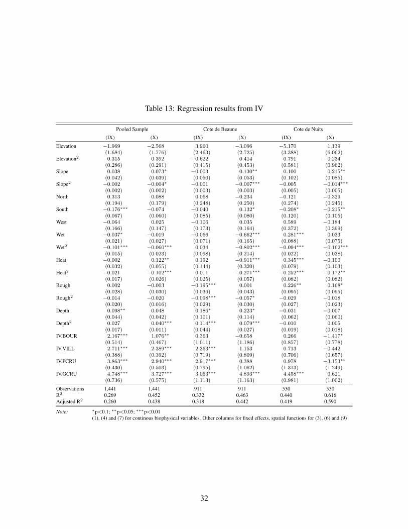
Table 13: Regression results from IV

Pooled Sample Cote de Beaune Cote de Nuits

(IX) (X) (IX) (X) (IX) (X)

Elevation −1.969 −2.568 3.960 −3.096 −5.170 1.139(1.684) (1.776) (2.463) (2.725) (3.388) (6.062)

Elevation2 0.315 0.392 −0.622 0.414 0.791 −0.234(0.286) (0.291) (0.415) (0.453) (0.581) (0.962)

Slope 0.038 0.073∗ −0.003 0.130∗∗ 0.100 0.215∗∗

(0.042) (0.039) (0.050) (0.053) (0.102) (0.085)Slope2 −0.002 −0.004∗ −0.001 −0.007∗∗∗ −0.005 −0.014∗∗∗

(0.002) (0.002) (0.003) (0.003) (0.005) (0.005)North 0.313 0.088 0.068 −0.234 −0.121 −0.329

(0.194) (0.179) (0.248) (0.250) (0.274) (0.245)South −0.176∗∗∗ −0.074 −0.040 0.132∗ −0.208∗ −0.215∗∗

(0.067) (0.060) (0.085) (0.080) (0.120) (0.105)West −0.064 0.025 −0.106 0.035 0.589 −0.184

(0.166) (0.147) (0.173) (0.164) (0.372) (0.399)Wet −0.037∗ −0.019 −0.066 −0.662∗∗∗ 0.281∗∗∗ 0.033

(0.021) (0.027) (0.071) (0.165) (0.088) (0.075)Wet2 −0.101∗∗∗ −0.060∗∗∗ 0.034 −0.802∗∗∗ −0.094∗∗∗ −0.162∗∗∗

(0.015) (0.023) (0.098) (0.214) (0.022) (0.038)Heat −0.002 0.122∗∗ 0.192 −0.911∗∗∗ 0.345∗∗∗ −0.100

(0.032) (0.055) (0.144) (0.320) (0.079) (0.103)Heat2 −0.021 −0.102∗∗∗ 0.011 −0.271∗∗∗ −0.252∗∗∗ −0.172∗∗

(0.017) (0.026) (0.025) (0.057) (0.082) (0.082)Rough 0.002 −0.003 −0.195∗∗∗ 0.001 0.226∗∗ 0.168∗

(0.028) (0.030) (0.036) (0.043) (0.095) (0.095)Rough2 −0.014 −0.020 −0.098∗∗∗ −0.057∗ −0.029 −0.018

(0.020) (0.016) (0.029) (0.030) (0.027) (0.023)Depth 0.098∗∗ 0.048 0.186∗ 0.223∗ −0.031 −0.007

(0.044) (0.042) (0.101) (0.114) (0.062) (0.060)Depth2 0.027 0.040∗∗∗ 0.114∗∗∗ 0.079∗∗∗ −0.010 0.005

(0.017) (0.011) (0.044) (0.027) (0.019) (0.018)IV.BOUR 2.167∗∗∗ 1.076∗∗ 0.363 −0.658 0.266 −1.417∗

(0.514) (0.467) (1.011) (1.186) (0.857) (0.778)IV.VILL 2.711∗∗∗ 2.389∗∗∗ 2.363∗∗∗ 1.153 0.713 −0.442

(0.388) (0.392) (0.719) (0.809) (0.706) (0.657)IV.PCRU 3.863∗∗∗ 2.940∗∗∗ 2.917∗∗∗ 0.388 0.978 −3.153∗∗

(0.430) (0.503) (0.795) (1.062) (1.313) (1.249)IV.GCRU 4.748∗∗∗ 3.727∗∗∗ 3.063∗∗∗ 4.893∗∗∗ 4.458∗∗∗ 0.621

(0.736) (0.575) (1.113) (1.163) (0.981) (1.002)

Observations 1,441 1,441 911 911 530 530R2 0.269 0.452 0.332 0.463 0.440 0.616Adjusted R2 0.260 0.438 0.318 0.442 0.419 0.590

Note: ∗p<0.1; ∗∗p<0.05; ∗∗∗p<0.01(1), (4) and (7) for continous biophysical variables. Other columns for fixed effects, spatial functions for (3), (6) and (9)

32