The Effects of Joining Multinational Supply Chains:New Evidence from Firm-to-Firm Linkages∗

Alonso Alfaro-Urena,† Isabela Manelici,‡ and Jose P. Vasquez§

October 2021

We study the effects of becoming a supplier to multinational corporations (MNCs) using tax data

tracking firm-to-firm transactions in Costa Rica. Event-study estimates reveal that domestic firms expe-

rience strong and persistent gains in performance after supplying to a first MNC buyer. Four years after,

domestic firms employ 26% more workers and have a 4 to 9% higher total factor productivity (TFP).

These effects are unlikely to be explained by demand effects or changes in tax compliance. Moreover,

suppliers experience a large drop in their sales to all other buyers except the first MNC buyer in the year

of the event, followed by a gradual recovery. The dynamics of adjustment in sales to others suggests

that firms face short-run capacity constraints that relax over time. Four years later, the sales to others

grow by 20%. Most of this growth comes from the acquisition of new buyers, which tend to be “better

buyers” (e.g., larger and with more stable supplier relationships). Finally, we collected survey data

from domestic firms and MNCs to provide further insights into the wide-ranging benefits of supplying

to MNCs. According to our surveys, these benefits range from better managerial practices to a better

reputation.

JEL Codes: F14, F23, F61, O12, D22, D24.

∗We thank Pol Antras, Larry Katz and three anonymous referees for their helpful and constructive comments.We are especially grateful to Andres Rodrıguez-Clare, Enrico Moretti, Ben Faber, Patrick Kline, Reed Walker,Cecile Gaubert, and Alan Auerbach, for their guidance and support. We have benefited from conversations withLaura Alfaro, David Atkin, Andrew Bernard, Emily Blanchard, Johannes Boehm, Juan Manuel Castro-Vincenzi,Davin Chor, Anca Cristea, Dave Donaldson, Thibault Fally, James Feyrer, Teresa Fort, Ted Miguel, EduardoMorales, Paul Novosad, Nina Pavcnik, James Sampi, James Sayre, Na’ama Shenhav, Felix Tintelnot, Nick Tsi-vanidis, Roman D. Zarate and numerous seminar participants. We also thank Marco Badilla and Brayan Segurafor their excellent research assistance. We owe special thanks to BCCR and its Economic Division in particular,for their hospitality during our visits. We also thank Procomer, COMEX, and CINDE for sharing data and insti-tutional knowledge. We acknowledge financial support from the Weiss Fund for Research in Development Eco-nomics, the research initiative “Private Enterprise Development in Low-Income Countries” (PEDL), the ClausenCenter for International Business and Policy, and the Center for Effective Global Action. The views expressedherein are solely those of the authors and are not necessarily those of BCCR or of any of the funding institutions.All results have been reviewed by BCCR to ensure no confidential information is disclosed.†Banco Central de Costa Rica (BCCR) and Universidad de Costa Rica. Email: alfaroua@bccr.fi.cr‡London School of Economics. Email: i.manelici@lse.ac.uk§London School of Economics. Email: j.p.vasquez@lse.ac.uk

1 Introduction

Governments around the world compete to attract foreign direct investment – typicallyin the form of affiliates of multinational corporations (MNCs) – through costly public pro-grams such as tax holidays or subsidized industrial infrastructure.1 The expectation of thesegovernments is that MNCs not only are high performers themselves but also help improve theperformance of domestic firms. This latter prospect is particularly appealing for developingcountries, where most firms are small and low-performing (Tybout, 2000). While direct supplychain linkages are not the only channel through which MNCs may improve the performanceof domestic firms, they are viewed as one of the most promising (Alfaro, 2017).

In this paper, we ask what are the effects of becoming a supplier to MNCs on domesticfirms. A complete answer to this question has so far proven elusive for three related reasons.First, it has been exceedingly difficult to observe direct business linkages between domesticsuppliers and MNCs in conventional data, especially for the entire economy. Past research hasthus relied on sector (or sector-by-region) level variation in the degree of foreign ownershipin downstream sectors. Second, firm supply linkages may be endogenous. Without observingactual linkages, it is difficult to tease out the direction of causality between supplying to MNCsand changes in firm performance. Third, the same inability to directly observe suppliers haslimited previous research from painting a complete picture of the effects of interest.

To make progress on these three challenges, we bring together a rich collection of micro-data from Costa Rica (henceforth, CR) that includes the near-universe of formal firm-to-firmtransactions in the country.2 This makes it possible to observe the actual linkages betweenMNCs and their domestic suppliers. Second, we adopt an event-study strategy to estimate theeffects of starting to supply to MNCs. We also probe the robustness of our baseline estimatesto four alternative control groups. Third, we provide a detailed account of the changes facedby first-time suppliers to MNCs (shortened to “first-time suppliers” hereafter). We begin withstandard measures of firm performance such as firm size or total factor productivity (TFP). Wethen leverage the firm-to-firm transaction data to document the adjustments in business withothers. We uncover changes in the average sales per buyer, the number of other buyers, andother buyers’ characteristics. We show that mere demand effects or changes in tax complianceare unlikely to explain our findings. Finally, for a more nuanced interpretation of our results,we conduct a survey of managers in a representative sample of domestic firms and MNCs.

The analysis proceeds in four steps. In the first step, we introduce the new database thatwe have assembled and the context. Most of our progress relies on the firm-to-firm transac-tion data collected by the Ministry of Finance since 2008. We match this data with corporateincome tax data and foreign ownership data, among others. We can then identify MNCs and

1The competition in investment incentives for MNCs is so high that governments are adopting ever more sophis-ticated approaches such as special tax incentives focused on intangible assets (UNCTAD, 2018a). Moreover, thenumber of Special Economic Zones – the mainstay of investment promotion and facilitation policies – rose from76 in 1986 (spread across 47 countries) to over 4,500 in 2018 (spread widely across the world) (UNCTAD, 2018b).

2The data cover all formal firm-to-firm transactions that in a year amount to more than 4,200 U.S. dollars. Duringour study period (2008–2017), this data was collected for general sales tax and corporate income tax enforcement.

1

domestic firms in buyer-supplier relationships and characterize these firms and relationships.In addition to this data advantage, ever since Intel’s entry in 1997, CR has attracted a large anddiverse set of MNCs. We exploit this feature in the heterogeneity analysis.

Our event of interest is the first time a domestic firm sells to an MNC in CR. We focuson events occurring between 2010 and 2015, for which we observe the transition of domesticfirms into their new role as suppliers of MNCs. During this period, 3,697 domestic firms startsupplying to one of 444 MNCs. On average, first-time suppliers employ 16.9 workers in theyears before their event. MNCs are notably larger, averaging 481 workers between 2008 and2017. Both sets of firms span a wide range of economic activities, though domestic suppliersare more likely to be found in services and MNCs in manufacturing. The first relationshipswith an MNC are plausibly consequential, as the average amount first sold to an MNC is62,400 U.S. dollars and represents 19% of all sales that year.

In the second step, we introduce our baseline event-study design to estimate the effectsof starting to supply to MNCs. The baseline sample includes both domestic firms that supplyfor the first time to an MNC in CR sometime between 2010 and 2015, and domestic firms thatnever supply to an MNC between 2008 and 2017 (henceforth referred to as “never-suppliers”).The identification assumption underlying this research design is that firms yet to supply toMNCs together with firms that started to supply MNCs in earlier periods form a crediblecounterfactual for first-time suppliers to MNCs, after we account for time-invariant differencesbetween firms and shocks common to firms in the same four-digit sector and province. As wecan estimate event-study coefficients for four years before an event, this method allows us totransparently show that first-time suppliers do not exhibit pre-trends in observables.

We first show that first-time suppliers experience strong and persistent improvementsin firm size. Four years after their first sale to an MNC buyer, firms have 33% higher sales,26% more employees, 22% more net assets, and 23% higher total input costs (all relative to theyear before the event). We then examine various measures of TFP, ranging from the residual ofOLS estimates of a Cobb–Douglas production function to an adapted version of the De Loecker(2013) estimation procedure (which accommodates endogenous productivity processes suchas learning by supplying to MNCs). After their event, domestic firms experience sizable andlasting gains in TFP, such that their TFP is 4 to 9% higher four years after. Finally, while ourTFP estimates may in part reflect markups, we provide evidence that strongly suggests that atleast part of the estimated TFP effects capture an actual increase in productivity and quality.

Next, with the aid of the firm-to-firm transaction data, we explore the business patternsof first-time suppliers with all their other buyers (all except the first MNC buyer). In the yearof the event, the sales to others decrease by 19%; of these sales, those made to other corporatebuyers (those buyers whose purchases must be reported in the firm-to-firm transaction forms)decrease by 75%. In time, however, the business with other buyers flourishes. Four yearsafter starting to supply to MNCs, sales to (corporate) buyers other than the first MNC buyerincrease by 20% (45%), the number of corporate buyers rises by 31%, and the average sales perbuyer increase by 14%.

2

Because we have merged the firm-to-firm transaction data with several other firm-leveldatasets, we can identify the buyers whose purchases have been most affected by the event.We first show that after the event, first-time suppliers to an MNC churn their old buyers morethan never-suppliers that are randomly assigned a fake event year. While most of their newbuyers are domestic, first-time suppliers also manage to secure new MNC buyers (other thantheir first MNC buyer). Four years after the event, first-time suppliers sell to 1.2 new MNCbuyers. On average, the new buyers of first-time suppliers are “better buyers,” in the sense ofbeing larger, more engaged in international trade, and having more stable supplier relations.

Our baseline results survive four alternative strategies that use different control groupsfor first-time suppliers. The first is an event-study design that leverages the rules of “Produc-tive Linkages,” a program that mediates linkages between MNCs and domestic suppliers. Pro-comer (the government agency implementing this program) assesses the ability of domesticfirms to supply to MNCs and assigns them scores. Based on these scores, Procomer proposes toMNCs shortlists of comparable contenders. These shortlists create the opportunity for a “win-ner vs. losers” design. One concern of the “Productive Linkages” exercise is its sample size.We overcome this concern via three matching techniques applied to the baseline sample ofeconomy-wide first-time linkages to an MNC: matching based on predicted Procomer scores,propensity score matching, and nearest-neighbor matching. These matching techniques sharewith “Productive Linkages” the benefit of generating contenders to each MNC deal. Reassur-ingly, all four alternative strategies deliver results consistent with our baseline results.

A lingering concern for identification is that firms may receive unobservable firm-specificshocks that affect both the timing of their first supplying relationship with an MNC and theirsubsequent performance. To alleviate this concern, we show that our results are robust toexcluding firms that had recently hired either a new manager (regardless of her previous em-ployment), a former worker for an MNC, or a supplier to an MNC (irrespective of her newposition). Finally, our results are robust to keeping only never-suppliers to MNCs that arenevertheless suppliers to a large domestic firm, dropping all never-suppliers to MNCs, vary-ing the fixed effects, and balancing the sample of first-time suppliers around the event year.

In the third step, we use the administrative data to further inform our interpretation ofthe baseline results. We first show that the long-term effects of “placebo” demand shocks (fromthe government, a large domestic buyer, or a domestic exporter) diverge decisively from thoseof demand shocks from an MNC. Second, the short-term fall in sales to others (which affectsboth first-time suppliers to MNCs and suppliers to other placebo buyers) suggests that domes-tic firms face steep short-run marginal cost curves – most likely due to capacity constraints orinflexible inputs. Third, we provide evidence that our results are unlikely to be explained bychanges in tax reporting after the first linkage with an MNC. Lastly, we show that, on average,domestic firms in manufacturing, who supply a core input to the MNC and/or have a strongerfirst interaction with the MNC, are those who gain most from their event. Moreover, it is mostuseful to supply MNCs in manufacturing and services, smaller MNC affiliates, and/or MNCswhose HQ country has a higher GDP per capita and better management practices.

3

In the fourth and final step, we rely on surveys we conducted on a representative sampleof MNCs and domestic suppliers. Both types of firms recognize how consequential it is fora domestic firm to start supplying to MNCs. After becoming suppliers to MNCs, most firmsundergo a series of interrelated changes, which include better managerial and organizationalpractices, expansions in product scope with higher-quality products, and improved reputa-tion. These changes arise from interactions during which MNCs communicate expectationsand advice, and from the effort exerted by new suppliers to deliver on their contracts. Overall,these insights match the story painted by the main results from the administrative data.

Our work is related to several literatures. At its core, this article contributes to an ex-tensive literature studying interventions aimed at improving firm performance in developingcountries. Woodruff (2018) notes that most of this literature focuses on interventions that al-leviate supply-side constraints (e.g., programs granting access to credit or training). Despitethe popularity of such interventions, literature reviews suggest that the evidence is mixed asto whether they can actually alter the long-term growth of firms.3 While notably scarcer, thereis increasing evidence that demand is an important determinant of (small) firm dynamics. Inparticular, improving access to foreign buyers – through trade4 or foreign direct investment(FDI) – is believed to hold great promise for firms in developing countries. The expectation isthat beyond increasing demand, foreign buyers provide valuable learning opportunities.

By studying the effects of selling to foreign buyers, this paper relates to a voluminousliterature on learning-from-exporting.5 In contrast to standard trade, global value chains orGVCs (joined upon starting to supply to an MNC) typically involve longer-term firm-to-firmrelationships. “This relational nature of GVCs makes them a particularly powerful vehiclefor technology transfer along the value chain. Firms have a shared interest in specializing inspecific tasks, exchanging technology, and learning from each other” (World Bank, 2020). Thisstronger alignment in incentives between buyers and suppliers, together with the increas-ing prevalence of GVCs, makes studying the effects of joining a GVC intrinsically interesting.Moreover, several other reasons justify this separate study. One such reason is the proximitybetween buyers and suppliers, which is likely to facilitate learning. Another is that exportingis only possible for firms selling tradables and competitive enough to overcome trade costs.Also, MNCs are plausibly more sophisticated buyers than the modal importer (Bernard et al.,2012). Finally, countries devise generous tax breaks to explicitly attract MNC affiliates. Esti-mating their effects on local firms is directly valuable for policy-makers, who can then comparethese estimates with those for alternative policies (e.g., export promotion).

By studying the effects of supplying to domestic affiliates of MNCs, this paper is alsoclosely related to a vast literature on the effects of FDI on firm performance.6 Papers on thistopic generally combine firm-level panel data with sector-level input-output (I-O) tables and

3For reviews on this strand of the literature, see Banerjee (2013) and McKenzie and Woodruff (2013).4De Loecker and Goldberg (2014) reviews the literature linking trade exposure to firm performance.5Atkin et al. (2017) provides causal evidence of learning-from-exporting for a sample of rug producers in Egypt.6For classic papers in the FDI literature, see Haddad and Harrison (1993); Aitken and Harrison (1999); Javorcik(2004); Alfaro et al. (2004); Haskel et al. (2007); Keller and Yeaple (2009). Contemporaneous papers on the widereffects of FDI include Abebe et al. (2020), Alfaro-Urena et al. (2019) and Mendez-Chacon and Van Patten (2020).

4

find that an increase in FDI at the sector (or sector-by-region) level is associated with increasesin standard measures of TFP of (nearby) domestic firms in upstream sectors (commonly re-ferred to as spillovers from backward linkages). Moving from variation in sector-level proxiesfor exposure to FDI to variation in the actual linkage status of a firm presents new opportuni-ties for precision and insight into the effects of joining MNC supply chains.7

Finally, this paper also relates to empirical work made possible by the recent availabil-ity of domestic firm-to-firm transaction data.8 We study in detail the effects of establishing afirst linkage with an MNC buyer. Four years after this first linkage, domestic firms substan-tially improve their sales to other buyers. Two-thirds of this improvement comes from theacquisition of new buyers. This echoes the finding that the number of buyers explains themajority of firm size heterogeneity (Bernard et al., 2020). Moreover, we use the firm-to-firmtransaction data in three novel ways. First, we show that first-time suppliers to MNCs notonly acquire new buyers, but they acquire buyers that are better-performing (e.g., larger andwith longer supplier relationships). Second, we compare the medium-run effects of demandshocks from MNCs against those from three types of placebo buyers (the government, largedomestic firms, and domestic exporters) and highlight the unique nature of MNCs as buyers.Third, we contrast the dynamics of adjustment for first-time suppliers to MNCs with that ofsuppliers to these placebo buyers. We bring evidence consistent with suppliers (to both MNCsand placebo buyers) having steep short-run marginal cost curves that flatten over time.9

This paper proceeds as follows. Section 2 describes the data and context. Section 3 in-troduces our baseline event-study strategy and four alternative strategies. Section 4.1 presentsour baseline results and Section 4.2 probes their robustness. Section 5 provides additional ev-idence from the administrative data to guide interpretation. Section 6 draws on surveys formore insights into the drivers of improvements in firm performance. Section 7 concludes.

2 Data and Description of Supplying Linkages

2.1 Data

Economy-wide administrative data. The main dataset tracks the near-universe of formalfirm-to-firm relationships in CR between 2008 and 2017. This information is collected by theMinistry of Finance of CR through the D-151 tax form. Firms must report the tax identifier(ID) of all their suppliers and buyers with whom they generate at least 2.5 million Costa Rican

7Using our firm-to-firm transaction data, we find that sector-level backward linkages predict less than 1% of theactual firm-level linkages with MNCs. This may explain why estimates of spillovers from backward linkagesvary broadly across studies, from strongly positive to negative (Havranek and Irsova, 2011). Table E1 (OnlineAppendix E.1) reports the TFP estimates for CR using sector-level and firm-level measures of backward link-ages (echoing the methodology of the previous FDI spillovers literature). We find that the standard measure ofbackward linkages is only significant when based on actual firm-level linkages but not on the sector-level ones.

8See, for example, Huneeus (2018), Brugues (2020), and Dhyne et al. (2020).9This insight resembles those of other papers that explain the interdependence of firm-level sales across marketsthrough increasing marginal costs (Almunia et al., 2020; Sun and Zhang, 2018; Ahn and McQuoid, 2017). We takeadvantage of the staggered timing of the event to estimate the marginal-cost elasticity at different time horizons.

5

colones (around 4,200 U.S. dollars) in transactions that year, in addition to the total amounttransacted. This declaration is compulsory not only to private businesses but to all actors in theeconomy (e.g., individuals providing professional services, public entities, etc.). Thanks to thethird-party reporting nature of the D-151 form, this data plays a crucial role in the enforcementof the general sales tax and corporate income tax.

We merge the firm-to-firm transaction data with the yearly corporate income tax returnsfrom the Ministry of Finance for the same 2008 to 2017 time period. These returns cover theuniverse of formal firms in the country and contain typical balance sheet variables (e.g., to-tal sales, net assets, input costs, etc.). We then add matched employer-employee data fromthe Costa Rican Social Security Fund, which tracks the labor earnings and occupations of allworkers engaged in formal employment.10 In some robustness checks, we also bring in dataon firm-level imports and exports from Costa Rican customs declarations.

Additionally, we construct a comprehensive dataset on the foreign ownership of firmsby cross-checking information from six different sources. The first three are annual surveysconducted by BCCR and inquiring on the foreign ownership of firms. These surveys tend tooversample large firms. The fourth source is the reporting of firms that are active under theFree Trade Zone regime. The fifth source is the organization responsible for drawing FDI toCR (CINDE), which provides information on the foreign ownership of firms they attracted.Finally, we bring in Orbis data, which has a high coverage of firms in CR and allows us toconfirm which foreign firms in the country are part of an MNC group.

A last step in building the final administrative dataset is to assign tax IDs to firm groupsand properly turn tax ID-level information into group-level information.11 Online AppendixA.1 discusses how we approach this step, in addition to providing more details on data con-struction and summary statistics for the administrative datasets mentioned above.

“Productive Linkages” data. Since 2001, Procomer (CR’s trade promotion agency) has im-plemented a matchmaking program called “Productive Linkages.” The program aims to insertlocal firms into export supply chains, where the exporter is usually an MNC affiliate. Procomerhas built a comprehensive database of local firms that are suitable and willing to supply toMNCs. Procomer staff visit firms and evaluate them on criteria that are typically unobserv-able in tax records but are nonetheless relevant to MNCs. Each firm is then assigned an overallscore. When an MNC approaches Procomer with an input need, Procomer identifies the sup-pliers that can produce that input, ranks them based on their score, and shares with the MNCa shortlist of the highest-ranked suppliers. Online Appendix A.2 describes the Procomer data.

We leverage the Procomer data in two ways. First, while the program was not designedas an experiment, by applying sensible restrictions to the universe of deals mediated by Pro-comer, we can retrieve a subset with a quasi-experimental setup. Specifically, we study the 31

10 Informal workers represent 27.4% of all workers in CR. While sizable, this share is smaller than the 53.1% averagefor Latin America (ILO, 2018). Section 5.3 and Online Appendix A.1.4 address the issue of informality.

11A firm can split its reporting across several tax IDs (e.g., by assigning all workers to one tax ID and all sales toanother). If they share ownership and make decisions as a unit, tax IDs should not be treated as independentfirms but should be aggregated into firm groups. Throughout the paper we use firms to refer to firm groups.

6

deals (i) that are first-time deals with an MNC for one of 31 domestic firms, (ii) that occur inour sample period (namely, between 2009 to 2015), and (iii) where all 84 contenders had notyet supplied to an MNC before the deal for which they were shortlisted. Second, we use theuniverse of Procomer scores to learn about their predictors from the administrative data. Wethen generate predicted Procomer scores for all firm-years in our economy-wide sample andapply a matching technique based on similarity in predicted Procomer scores.

Survey data. In 2018, we conducted surveys of both MNCs and their domestic suppliers.Our main objective was to shed light on typically unobservable aspects of relationships be-tween the two types of firms. The surveys were administered in two versions: a longer fieldsurvey conducted at the main location of the firm and a shorter web-based one. Core questionswere mirrored between surveys to both domestic firms and MNCs. Given the retrospective na-ture of some of the topics covered, the ideal respondent was the founder of the domestic firmand the supply chain manager of the MNC. The need to reach specific employees compoundedthe already difficult task of establishing a first contact with these firms.

We gathered responses from a total of 164 firms, of which 38 were surveyed in person and126 online. 106 respondents are domestic suppliers to MNCs and 58 are MNCs based in CR.Combined, the 164 responses from buyers and sellers cover at least one side of the buyer-sellerpair for about 20% of the pairs of interest. Comparing the firms with and without a responsesuggests that a response bias is unlikely. See Online Appendix F for more details.

2.2 Description of MNCs, Domestic Suppliers, and Their First Linkage

MNCs in CR. We start from the 2,156 firms in CR that belong to corporate groups whereat least one firm is partially foreign-owned.12 From this set of firms, we create three mutuallyexclusive subsets: firms that are fully domestically-owned (despite being part of a corporategroup where another firm is partially foreign-owned), firms that are themselves at least par-tially foreign-owned but whose median employment across all years of activity in the countryis under 100, and firms that are themselves at least partially foreign-owned and whose medianemployment is over 100. We study the 622 firms in the third category.13

All the 622 firms we focus on are MNC affiliates, with known global ultimate ownershipand a substantial affiliate presence in CR. We use the customary definition of an MNC, as “anenterprise that controls and manages production establishments/plants located in at least twocountries” (see Antras and Yeaple, 2014). Our size threshold also enables us to circumventissues related to FDI statistics, such as the rising use of shell companies. These 622 firmsemploy 76% of the workers and export 91% of the totals across firms in the three categories

12A corporate group is a set of firms that share ownership, but do not necessarily behave as one business. Forinstance, some firms in the same corporate group may operate in different economic sectors.

13The typical foreign-owned firm in the second category is not an MNC affiliate but a single location firm thatserves local demand, either in service sectors (e.g., hotels) or sectors with low local input requirements (e.g.,import/export retail or real estate agencies). While our baseline results pertain to the 100-worker size restrictionfor foreign-owned firms, we show in Online Appendix D.4 that results are robust to removing it and includingfirms in the second category as well.

7

combined (see Online Appendix A.1.3).From the universe of firm-to-firm transactions in CR, we learn that between 2010 and

2015, 444 of these 622 MNCs became the first MNC buyer from one of 3,697 domestic firms.46% of the 444 MNCs are from the United States, with the other 54% coming mainly fromeither Latin America or Western Europe. While manufacturing is the most frequent sector(covering 38% of the 444 MNCs), the remaining 62% of MNCs fall into sectors as diverse asretail, agriculture, and information and communication. For more detailed summary statisticson these MNCs, see Tables B1 and B2 in Online Appendix B.

Domestic suppliers to MNCs. Among all the domestic firms in CR, we restrict our attentionto those with at least a median of three workers and median yearly revenues of 50,000 U.S.dollars (CPI-deflated to 2013 dollars) across all years of activity. We remove firms that are state-owned, registered as households, NGOs, or part of the financial, construction, and educationsectors.14 This leaves us with 24,370 firms. Of these firms, we use the firm-to-firm transactiondata between 2008 and 2017 to identify and keep only two types of firms: the 3,697 firms thatbecome first-time suppliers to an MNC sometime between 2010 and 2015,15 and the 14,338firms never supplying to an MNC between 2008 and 2017. Our interest lies in the firms in thefirst category, but we also use firms in the second category to construct counterfactuals.

For the 3,697 first-time suppliers to an MNC, the average number of workers in the yearsbefore the event is 16.9. Around 11% of these firms operate in manufacturing, while around32% work in wholesale and retail trade (including repair and maintenance). Among the ser-vice sectors, the most common sectors are professional, scientific and technical services (14%),administrative and support services (10%), transportation and storage (9%), and accommoda-tion and food services (6%). For more summary statistics on the first-time suppliers (e.g., ontheir productivity, trade activity, age, number of buyers) see Table B3 in Online Appendix B.

Relationships between MNCs and their domestic suppliers. In CR, MNCs and domestic firmscan establish a buyer-seller relationship either independently, unmediated by any governmentinstitution, or mediated by Procomer through the “Productive Linkages” program. The aim ofprograms such as “Productive Linkages” is not to replace unmediated market-based linkagesbetween MNCs and domestic suppliers with linkages mediated by the program, but to createadditional opportunities for linkages (e.g., by lowering informational barriers on the capabil-ities of domestic suppliers). This program mediates only 1% of both the number and valueof linkages between MNCs and domestic suppliers occurring economy-wide in CR. For thisreason, we prioritize the analysis of unmediated relationships.

As mentioned above, we find 3,697 domestic firms that supply to an MNC for the first

14While we justify these restrictions in Online Appendix A.1, our baseline results are robust to discarding them (seediscussion in Section 4.2.2 and corresponding tables in Online Appendix D.4).

15We start in 2010 to ensure we measure correctly the first year when a firm supplies an MNC. After 2015, we areno longer able to observe at least two years after each first-time linkage. Also, there are 3,813 domestic firms thatbecame first-time suppliers to 471 MNCs. However, in the main event-study regression (1) studying the impacton total sales, only 3,697 of these domestic firms are used in the estimation, with the rest being dropped due tothe fine set of fixed effects used. For consistency, we present summary statistics only for those 3,697 firms andtheir associated 444 first MNC buyers.

8

time sometime between 2010 and 2015, and do so in an unmediated fashion. We refer to thesefirst-time supplying instances as (unmediated economy-wide) events. Across these events, theaverage amount first sold to an MNC is 62,400 U.S. dollars and represents 19% of all sales thatyear. While the average relationship of first-time suppliers lasts 1.99 years, the relationshipwith the first MNC buyer lasts on average 2.77 years. This suggests that the relationship withthe first MNC buyer is plausibly consequential for the supplier. For more summary statisticson the events, see Tables B4 and B5 in Online Appendix B.

3 Empirical Strategy

3.1 Baseline Empirical Strategy: Economy-Wide Event Studies

In what follows we present our baseline empirical strategy to study the effects of becom-ing a first-time supplier to an MNC in CR. Between 2010 and 2015, 3,697 such events occuracross the Costa Rican economy. More specifically, we estimate the following event-studyspecification:

yit = αi + λspt +C

∑k=C

θkDkit + εit, (1)

where yit is an outcome of firm i in calendar year t, αi is a firm fixed effect, and λspt are four-digit sector × province × calendar year fixed effects. We define the event-time dummies asDk

it := 1[t = τi + k] ∀k ∈ (C, C), DCit = 1[t ≥ τi + C], and DC

it = 1[t ≤ τi + C], where 1[.] isthe indicator function and τi is the first year when firm i sells to an MNC. εit is an error term.We normalize θ-1 = 0 and set C = −5 and C = +5. We cluster standard errors at the two-digitsector × province level.

Our baseline economy-wide regressions use a sample that includes both domestic firmsthat become first-time suppliers to an MNC sometime between 2010 and 2015 and domesticfirms that never supply to an MNC between 2008 and 2017. Identification of the event-studycoefficients θk hinges on the assumption that firms yet to supply to MNCs and firms thatstarted to supply in earlier years form a credible counterfactual for firms that start supplying toMNCs, after accounting for time-invariant differences between firms and common sector-by-province-by-year shocks.16 The panel data allows us to consistently estimate treatment effectswithout assuming treatment exogeneity and without an instrumental variable, provided thatthe treatment varies over time and is uncorrelated with transitory firm-specific shocks thatcan determine outcomes (Wooldridge, 2002; Blundell and Dias, 2009). Section 4.2.2 providesevidence in support of these identification assumptions.

16This design is not challenged by selection on levels, observable or not. For instance, even before starting tosupply to MNCs, first-time suppliers employ on average 19% more workers than never-suppliers in the samefour-digit sector and province. In addition, a consistent estimate of the average treatment effect requires thattreated and control firms experience the same macro shocks (Blundell and Dias, 2009). Differential trends mightarise if treated and control units operate in different markets. We limit control firms to nearby firms in the samefour-digit sector to account for common shocks, such as those to factor markets or transportation networks.

9

3.2 Alternative Empirical Strategies

3.2.1 “Productive Linkages” Event Studies

The rules of the “Productive Linkages” program generate quasi-experimental variationin opportunities to supply to MNCs among firms shortlisted for a given deal with an MNC.Procomer undertakes thorough evaluations of domestic firms willing to supply to MNCs andassigns them an overall score of readiness to do so. These scores reflect information that isrelevant to MNCs, yet not available in typical tax data (e.g., whether the firm employs at leastone English speaker). Based on scores, Procomer proposes shortlists of candidates to MNCs.17

The “Productive Linkages” event-study is a generalized triple-difference design wherefirms experience a first deal with an MNC in different years. We modify equation (1) to allowfor an extra interaction between event dummies Dk

idt and an indicator dummy of winning deald, 1{Winner}id. We label the winner and losers of the same deal with the same d subscript. Weinvestigate the effect of being considered for deal d on both the winner and losers of that dealby running the following regression:

yidt = αi + γd + λt +C

∑k=C

θLk Dk

idt +C

∑k=C

θDiffk 1{Winner}idDk

idt + εidt, (2)

where yidt is the outcome of firm i part of deal d in year t, λt is the calendar year fixed effect,and 1{Winner}id is an indicator function that equals 1 if firm i is the winner of deal d. γd aredeal fixed effects that force the effects on the winner to be measured with respect to those onthe actual contenders to the same deal. Our coefficients of interest are θL

k and θDiffk , which are

interpreted as the effect of the event on the losers and on the difference in outcomes betweenwinners and losers, respectively. All other variables are defined the same as for equation (1).

Identification relies on the assumption that shortlisted firms missing a deal with an MNCoffer a valid counterfactual to what would have happened with the winners’ performance hadthey not won the deal. As we observe the scores behind the ranking shared with MNCs, wecan compare the scores of winners and losers. In Online Appendix A.2.2 we provide evidenceindicating that the only meaningful difference between winners and losers is the timing of afirst deal with an MNC (as opposed to ex-ante differences in scores or other observables).

3.2.2 Event Studies Combined with Matching Estimators

One advantage of the baseline exercise with economy-wide event studies is its samplesize of 3,697 treated firms (in contrast to the 31 treated firms in the “Productive Linkages”exercise). Where the “Productive Linkages” exercise dominates the baseline exercise is in itsability to compare the outcomes of treated firms with the contemporaneous outcomes of similarfirms (as witnessed by their scores). In what follows, we present three techniques which com-bine these two advantages, i.e., which use the same sample of 3,697 economy-wide first-time

17Online Appendix A.2.1 provides more background information on the program history and functioning.

10

suppliers as the treated firms and compare their outcomes to the contemporaneous outcomesof control firms which are similar in one of three ways defined below.

Matching by predicted Procomer scores. This exercise starts from the 630 Procomer scoresassigned to 613 distinct firms in the years with administrative data (2008–2017). We regressthe Procomer score of a firm-year on fourteen potential predictors of that score (in addition totwenty broad sector fixed effects). Among the predictors are measures of firm size, the shareof college-educated workers, indicators for whether the firm is an exporter, employs workerswith experience at an MNC or supplies to a big domestic firm. We then use the estimatedcoefficients (see Table D2 in Online Appendix D.1) to predict Procomer scores for all firm-yearsin the full economy-wide sample. The control group for each first-time supplier contains thethree never-suppliers in the same four-digit sector that have the closest predicted Procomerscore to the one of the first-time supplier in its event year.

We then estimate for each outcome a modified version of the event-study specification inequation (1). The modification involves an extra interaction between event-time dummies andan indicator dummy of becoming a first-time supplier in the year of the event. This versionof equation (1) resembles equation (2) in that they both include a contemporaneous “winnervs. losers” comparison captured by the θ

Di f fk coefficients (estimating the effect of the event on

the difference in outcomes between the first-time suppliers and their control group, this timeconstructed based on the predicted Procomer score). As in equation (1), we include firm fixedeffects and four-digit sector × province × calendar year fixed effects.

Propensity score matching. We also implement the standard propensity score matching. Inour case, the propensity score – denoted by e(Xit) – is the conditional probability that firm iis chosen as a first-time supplier to an MNC in year t. To obtain e(Xit) we estimate a year-by-year flexible probit model for the full economy-wide sample. Xit includes the same character-istics of firm i in year t that we used to predict the Procomer scores in the matching methoddescribed above (in addition to four-digit sector, year and province fixed effects). Table D2(Online Appendix D.1) reports the results of the probit regression. We fix as the control groupof a given first-time supplier the three never-suppliers in its four-digit sector with the clos-est propensity score in the event year of that supplier. We then compare the outcomes of alleconomy-wide first-time suppliers to those of firms in their personalized control group. Wedo so by estimating the same modified version of equation (1) described above.

Nearest neighbors matching. In this exercise, we match first-time suppliers with controlfirms that did not supply to MNCs based on the similarity of their pre-event outcomes. Foreach first-time supplier, potential control firm and outcome, we compute a loss function equalto the sum of squares of the deviations of the standardized outcome of the first-time supplierfrom that of the potential control firm. This sum is across the three years before the event,where the deviation of each year is equally weighted. We then select as the “nearest neigh-bors” the three firms in the four-digit sector of the first-time supplier with the lowest valueof the loss function. These nearest neighbors serve as a counterfactual for first-time suppliers

11

in a generalized “difference-in-differences” estimation. Namely, our difference-in-differencesestimate reflects the average difference in the outcomes of the first-time suppliers and theircontrols in the same event year, relative to the average difference in the year leading up to afirst-time supplying event. For more details on this method, see Online Appendix D.1.1.

4 First-Time Suppliers to MNCs Improve Their Performance

4.1 Baseline Economy-Wide Event-Study Results

4.1.1 Standard Measures of Firm Performance

In what follows we rely on the event-study specification (1) and the economy-wide fullsample to estimate the effects of starting to supply to an MNC on firm size and measures ofTFP. These results characterize the 3,697 domestic firms that become first-time suppliers to anMNC in CR sometime between 2010 and 2015.

Firm size. Panels 1a-1d of Figure 1 plot the event-study coefficients for log total sales,number of workers, net assets (as a proxy for capital),18 and input costs (as a proxy for materi-als). Reassuringly, we find no evidence of selection into supplying based on past firm growth.It is only after firms start supplying to MNCs that they experience strong and lasting growth.This growth already starts in the year of their first transaction with an MNC, with the averagegrowth that year relative to the previous year being 16% in sales, 6% in the number of workers,and 9% in input costs. Net assets react with a one-year lag. Firms keep growing over the nextyears until reaching a plateau at 33% higher sales, 26% more workers, 22% more assets, and23% higher input costs. Table 1 provides additional details.

The magnitude and long-run nature of these effects are noteworthy. In other settingswhere firms receive demand shocks that are comparable or larger, firms do not grow as much.For instance, Atkin et al. (2017) finds that Egyptian microenterprises that receive large exportorders for rugs (with cumulative payments of 155,682 U.S. dollars for 2.5 years of work) didnot increase their employment and capital usage. Similarly, supply-side interventions such asbusiness training can also fail to boost firm scale (Karlan and Valdivia, 2011).

Measures of TFP. We first estimate TFP using OLS, assuming either a Cobb–Douglas ortranslog technology. To this end, we extend the specification (1) by using log sales as the out-come variable and the logs of the number of workers, net assets (as a proxy for capital), andinput costs (as a proxy for materials) as time-varying controls.19 As OLS does not accountfor the potential endogeneity of input choices, we also use the methods proposed by Levin-sohn and Petrin (2003) and Ackerberg et al. (2015). In cases without input and output price

18 The net assets variable is the sum of (i) cash and other liquid assets, (ii) shares/stocks, (iii) inventories, and (iv)total fixed assets. In the terminology of the Costa Rican Ministry of Finance, the “net” designation means that thefixed assets part of this variable is already net of depreciation, amortization, and depletion.

19 We use net instead of fixed assets because there are fewer missing or zero firm-year values for net assets. TFPestimates using fixed assets are virtually identical and are available upon request.

12

variations correlated with the event, these two methods provide credible estimates of true TFP.Additionally, we adapt the TFP estimation procedure of De Loecker (2013) such that the

endogenous TFP process that is accommodated by this procedure is no longer learning fromexporting, but learning from supplying to an MNC. With this adapted method, we can explorethe possibility that supplying to an MNC shapes a firm’s future TFP while allowing other firm-level actions (e.g., investment decisions) to also impact future TFP. This method addresses thepotential bias of ignoring a firm’s MNC-supplying experience in the underlying TFP process(bias that might affect standard proxy estimators such as Levinsohn and Petrin, 2003).

Panels 1e and 1f in Figure 1 summarize the TFP results and Table 1 provides more details.Reassuringly, firms that start supplying to MNCs do not display a history of TFP growth. Aftertheir events, however, suppliers exhibit large increases in TFP, such that four years later, TFPis 4 to 9% higher than in the year before the event (depending on the estimation procedure).

Markup effects (or lack thereof). The TFP estimates above might be upward biased if first-time suppliers to MNCs start charging higher markups – to the first MNC buyer alone or toother buyers as well. This can happen if supplying to MNCs leads to quality improvements,higher-quality goods carry higher markups (as in Atkin et al., 2015), and there are no coun-tervailing forces that tend to compress markups (such as switching to buyers with greaterbargaining power or markets with tougher competition, as in Acemoglu and Tahbaz-Salehi,2020; Alviarez et al., 2020; Mayer et al., 2014). We will argue that while the first two conditionsmay be met, the third condition is unlikely to be met in our empirical setting.

Before proceeding with our evidence, an important caveat is in order. Namely, lackingdata on prices and quantities for domestic transactions makes it difficult to rule out definitivelythe possibility that part of the estimated TFP gains reflects higher markups. That said, in whatfollows, we provide several pieces of evidence that strongly suggest that at least part of theestimated TFP effects capture an actual increase in productivity and/or quality.

First, in Table C1 (Online Appendix C) we use the empirical models of De Loecker andWarzynski (2012) and Sampi et al. (2021)20 to show unchanged (or declining) average markupsfor first-time suppliers to MNCs. This evidence is in line with our surveys, which point to thestrong bargaining power of MNCs and their ability to squeeze suppliers’ margins.21 Previousresearch reports similar findings (e.g., Javorcik, 2008; Javorcik et al., 2008).22 Our surveys alsosuggest that even when the quality of the domestic firms’ products increases after the firstMNC linkage, these higher-quality products are sold at unchanged or falling prices (to boththe first MNC buyer and other buyers). See Section 6 for details.

20Sampi et al. (2021) provide a work-around solution to the concerns raised by Bond et al. (2021) on the interpreta-tion of markups estimated using the ratio of the output elasticity of a variable input to that inputs cost share inrevenue (such as in De Loecker and Warzynski, 2012). Moreover, the Sampi et al. (2021) method is appropriate insettings where measuring the change in markups (as opposed to their level) is enough.

21MNCs have privileged access to imports (e.g., MNCs in Free Trade Zones are exempted from customs duties)and leverage their corporate commodity managers to learn about suppliers abroad. Moreover, the leading in-ternational suppliers of MNCs tend to pursue their buyers as they open new affiliates (a practice called followsourcing). The larger the MNC, the more likely it is to have these sourcing advantages. These factors combinedleave little room for domestic suppliers to obtain higher markups from MNCs.

22For instance, 40% of suppliers to MNCs in the Czech Republic had to lower prices by 1 to 30% (Javorcik, 2008).

13

Second, as we will see in the next section, starting to supply to MNCs improves the salesof domestic firms made to other buyers. Suppose first-time suppliers learn from the first MNCbuyer how to produce higher-quality products, and their other buyers also demand such prod-ucts. One might be concerned that the increase in sales to others captures only higher markupson those higher-quality products. For plausible values of the demand elasticity (specifically,for values lower than -1), without a fall in marginal costs and/or an increase in the demandshifter (product quality or appeal) that are large enough to compensate for the higher markups,higher markups alone would lead to a fall in sales in others. Online Appendix E.3.3 containsthe formal argument. Moreover, the tendency of higher markups on higher-quality goods maybe offset by the greater bargaining power of the new buyers of first-time suppliers, who (asshown in the next section) are larger and more internationally exposed.

4.1.2 Business with Other Buyers

With the aid of the firm-to-firm transaction data, we now explore the patterns of businessof first-time suppliers with all buyers except the first MNC buyer. This exploration has twogoals. First, it addresses the natural concern that the firm growth documented so far is owedprimarily to the addition of the new MNC buyer. Second, we will argue that what happens tothe business of first-time suppliers in other markets (in this case, with all their other buyers inCR) is informative on both the mechanisms behind the effects of a first linkage with an MNCand firm fundamentals more broadly (such as the marginal cost elasticity).

Let us first define a couple of objects of interest. The “sales to others” are equal to totalsales minus the sales to the first MNC buyer, where the total sales come from the corporateincome tax returns and the sales to the first MNC buyer come from the firm-to-firm transactiondata. The “corporate buyers” of a firm in a given year are its buyers reported in the firm-to-firm transaction data, i.e., firms in CR whose purchases of goods or services from that firmexceed 4,200 U.S. dollars that year. The “total corporate sales” are equal to the sum acrossthe sales to all corporate buyers in the firm-to-firm transaction data. The “corporate sales toothers” exclude the sales to the first MNC buyer. Aside from total corporate sales, total salescontain exports and sales to end consumers and to firms in CR whose purchases that year sumup to less than the reporting threshold. We call this difference “non-corporate sales.”

In addition to the pattern of total sales (sales to all buyers), Figure 2 shows the patternsof sales to all buyers except the first MNC buyer, all corporate buyers, and all corporate buyersexcept the first MNC buyer. Across the four types of buyers, we do not find evidence of differ-ential trends in sales before the event of a first sale to an MNC. However, we find large andlasting increases in the four types of sales after the event. Most importantly, these increases arenot mechanical as they survive the exclusion of the sales to the first MNC buyer. Four yearsafter the event, sales to others increase by 20%, while corporate sales to others increase by

14

45%.23 Table 2 provides details and robustness checks (e.g., showing that the baseline resultsare not driven by demand from buyers who are themselves new suppliers to MNCs).

Extensive vs. intensive margin responses. Next, we ask whether these changes in sales toothers materialize primarily along the extensive or the intensive margin. Panel 2e in Figure2 depicts the extensive margin response (i.e., the effect of the event on the log number ofcorporate buyers, except the first MNC buyer), while panel 2f looks into the intensive marginresponse (i.e., the effect on the average value of transactions across all other corporate buyers).Reassuringly, in the years preceding the first linkage with an MNC, we find no differentialtrends in either the number of corporate buyers or the average sales to others. After the event,however, both margins react. Four years later, first-time suppliers have 31% more corporatebuyers and average transactions are 14% larger than in the year before the event. Hence, ofthe 45% increase in corporate sales to others, the intensive (extensive) margin accounts for one(two) third(s) of the increase.24 Table 2 provides more details.

Short- vs. medium-run adjustments. The focus on the effects four years after the eventconceals striking short-run adjustments. Namely, in the year of the event, the sales to othersdecrease by 19%, the corporate sales to others by 75%, and the non-corporate sales to othersby 9%. Most of the 75% drop in corporate sales to others occurs along the intensive margin.Specifically, the average sales to others drop by 78% in the year of the event, while the numberof other buyers increases by a modest 3%. For details, see Table 2.

These findings suggest that firms are capacity-constrained in the short-term. While ca-pacity constraints can encompass more factors than what is captured by our net assets variable(say managerial attention), the finding that the net assets react with a one-year lag is consistentwith the idea that firms cannot adjust fixed inputs in real-time. The short-term need to scaledown the business with other buyers is one to which we will return in Section 5.2.

Changes in buyers’ characteristics. Our data merge allows us to go beyond tracking re-sponses in the business with others, where the “others” are left anonymous. Figure C1 (OnlineAppendix C), breaks down the corporate sales of first-time suppliers to an MNC by whethera buyer is old or new and an MNC or not. We define an “old buyer” as a buyer to whomthe first-time supplier sells by the event year. To provide a reference point, we also studynever-suppliers that are randomly assigned a fake event year between 2010 and 2015. Fouryears after the event, around 60% of the corporate sales of first-time suppliers go to new buy-ers acquired after the event. This percentage stands in contrast to slightly more than 50%for never-suppliers. Hence, while the churning of old buyers is not a pattern limited to first-time suppliers, new buyers are clearly more important for them than for never-suppliers. For

23Naturally, the discrepancy between the increases in the sales to others and corporate sales to others is driven bythe behavior of non-corporate sales. Four years after the event, non-corporate sales increased by 16%, makingthe share of non-corporate sales out of all sales to others fall by 7%. Hence, first-time suppliers have shifted theirsales more toward corporate buyers, i.e., toward firms with purchases above 4,200 U.S. dollars per year.

24Our findings of increased sales to others suggest that these other buyers may have benefited as well from theupgrades of the first-time suppliers (as in Kee, 2015). While potential gains to domestic buyers are relevant toany estimation of the aggregate effects of MNCs, they are beyond the scope of this paper.

15

legibility, the “domestic buyers” in Figure C1 bundle domestic firms, non-MNC but partiallyforeign-owned firms, and the government. While most corporate sales to new buyers are tonew “domestic buyers,” first-time suppliers also acquire new MNC buyers.25 Four years afterthe event, on average, 6% of the sales of first-time suppliers go to 1.2 new MNC buyers.26

Table 4 provides additional evidence that joining the supply chain of an MNC induceschanges in the buyer characteristics of first-time suppliers. We first find that four years af-ter acquiring a first MNC buyer, domestic firms sell to buyers in 18% (21%) more two-digit(four-digit) sectors. Meanwhile, first-time suppliers do not buy from more two-digit (four-digit) sectors. Next, we learn that the sales of first-time suppliers (four years after) are madeto buyers with 49% more workers, 53% higher sales, 30% more suppliers, and 40% more buy-ers. First-time suppliers tend to sell to buyers who are slightly more internationally exposed,as proxied by their share of exports in total sales and imports in total inputs. Finally, first-time suppliers sell to buyers with more substantial relationships with all their suppliers, asmeasured by the 19% higher average value of transactions and 8% longer relationships.27

Overall, our evidence on the persistent boosts in performance with other buyers (in par-ticular, on the improved ability to acquire new buyers), the changing composition of sales bybuyer type (e.g., from old to new), and the better-performing new buyers (e.g., larger size orlonger supplier relationships) of first-time suppliers to MNCs are consistent with improve-ments in productivity, product scope and quality, and reputation for first-time suppliers.

4.2 Robustness Checks to the Baseline Results

4.2.1 Results from Alternative Empirical Strategies

Table 3 presents the event-study estimates obtained from the four alternative strategiesdescribed in Section 3.2, namely the “Productive Linkages” strategy and the three matching es-timators applied to the economy-wide sample. Table 3 focuses on three of our main outcomes:

25Figure C1 has to focus on corporate sales, as it is only with the firm-to-firm transaction data that one can establishwhether a buyer is old or new and an MNC or not. In Figure C2 we study total sales, which include the non-corporate sales (the sum of exports and the part of local sales not reported in the firm-to-firm transaction data).Figure C2 disaggregates the total sales of first-time suppliers into a more narrowly-defined set of buyers: thegovernment, domestic firms and consumers, non-MNC partially foreign-owned firms, MNCs, and exports. Here,the sales to domestic firms and consumers are computed as the residual from the total sales minus the sales toMNCs, sales to partially foreign-owned firms that are not MNCs, exports, and sales to the government. We findthat most of the increase in total sales after the event stems from sales to domestic firms and consumers (this time,more narrowly defined). Other buyers also tend to increase their purchases, though more modestly.

26Tables B4 and B5 (Online Appendix B) provide more details on post-event relationships with MNCs. Moreover,Tables C2 and C3 (Online Appendix C) expand our event-study analysis to study the effects of subsequent MNCbuyers. Namely, in these tables, a year with an event is any year in which a domestic firm starts supplying toa new MNC buyer (the first MNC buyer or a subsequent one). Table C2 splits the baseline sample of first-timesuppliers to MNCs based on their total number of years with events. The more years with events a first-timesupplier has, the stronger its overall growth in size and TFP. Table C3 compares the pooled (before vs. after)change in total sales and TFP after each new year with an event. After each additional year with an event, firmsexperience a slight increase (decrease) in the pooled change in sales (TFP). While caution is warranted in drawingcausal inferences, these findings are suggestive of the value of expanding one’s portfolio of MNC buyers.

27To avoid mechanical results, we exclude the first MNC buyer from all results in Table 4. Changes in firm size alsodo not explain these results, as we have already controlled for the suppliers’ contemporaneous total sales.

16

total sales, TFP residual from an OLS production function estimation under a Cobb–Douglastechnology, and the corporate sales to others.28 We contrast the estimates for each alternativestrategy and outcome with our baseline estimates summarized in Tables 1 and 2.

Reassuringly, across methods and outcomes, we find either a lack of or sporadic pre-trends. Moreover, all four sets of event-study estimates display the same qualitative patternsas the baseline estimates (e.g., the extensive margin response of new buyers is the leadingdriver of the rise in sales to other buyers). While the point estimates tend to vary across em-pirical strategies, the confidence intervals overlap for most outcomes and event years. Thisis true despite these alternative approaches using control groups built on either more infor-mation than what is typically observed in administrative data (but captured in the Procomerscore) or stronger predictors of supplying linkages than the sector and province of a firm.Overall, it is encouraging that these four alternative approaches support our baseline results.

4.2.2 More Robustness Checks to the Baseline Economy-Wide Event Studies

Our baseline economy-wide regressions allow in the sample of control firms the “never-suppliers,” i.e., domestic firms never observed as supplying to an MNC throughout 2008 to2017. To assuage concerns over the similarity between first-time suppliers and never-suppliersto MNCs, Online Appendix D.2 explores the implications of dropping from the control groupall or part of the never-suppliers. Table D4 shows that the baseline estimates hold up to drop-ping all the never-suppliers. This suggests that the driver of our baseline results is the stag-gered timing of the event, and not the contrast to never-suppliers. In Table D5, we only excludethe never-suppliers to an MNC that are also never-suppliers to a large domestic firm through-out 2008 to 2017. This exercise therefore accepts in the control group only firms having sold toa large buyer. These new event-study estimates remain similar to the baseline ones.

There is one important threat to identification that is not addressed by our analysis thusfar: firms may experience unobservable firm-specific shocks that affect both the timing of theirfirst supplying relationship with an MNC and their subsequent performance. While not allsuch shocks need to be embodied in new employees, the hiring of new influential employeesbefore the first sale to an MNC is among the most plausible confounding factors. Problematicinfluential employees would need to be able to both establish the first contract with an MNCand improve firm performance. In Online Appendix D.3 we investigate this scenario usingmatched employer-employee data from the Costa Rican Social Security Fund.

We first consider the hiring of a new manager, as managers can impact overall firm per-formance. We first define managers as the firm’s top two earners. Alternatively, we take asmanagers workers whose occupation is categorized as managerial by ISCO-08. From the base-line sample of first-time suppliers, we then drop those having hired a new manager in eitherthe year of their event or the year before. We also consider hiring workers straight from anMNC or a supplier to an MNC as another plausibly concerning event. Such workers may both

28Table D1 (Online Appendix D.1) reports the estimates for the number of workers, the number of other buyers,and the average sales to other buyers.

17

use their MNC contacts to generate a first MNC contract for their new employer and transferknowledge acquired during their previous employment (improving the performance of theirnew employer). We then exclude from the baseline sample of first-time suppliers those whohave hired a new worker – in either the year of their event or the year before – whose previ-ous main employer was one of the 622 MNC affiliates in CR (or, in a separate exercise, was asupplier to one of these MNCs).29 Our findings survive all of these four exclusions. While it isimpossible to fully dismiss the threat of firm-specific shocks with the problematic traits men-tioned above, this evidence suggests that worker-embodied shocks are unlikely confounders.

Finally, we probe the sensitivity of our results to relaxing the restrictions imposed ontothe main sample described in Section 2.2. In Online Appendix D.4 we relax both one-at-a-time and simultaneously the size and sectoral restrictions set on either the domestic firms orMNCs in the baseline sample. Across variables and sample variants, our main takeaways fromTables 1 and 2 remain unaffected. Moreover, our key takeaways remain qualitatively similaracross significant variations in fixed effects, including fixed effects that control for trends inmore disaggregated geographic units (see Online Appendix D.5). Results also remain largelyunchanged for a balanced sample in event time (see Online Appendix D.6). These alternativeexercises corroborate the robustness of our baseline event-study specification and sample.

5 More Evidence from Admin Data to Guide Interpretation

5.1 MNC Demand Shocks Differ from Those from Large Domestic Buyers

We now carry out three placebo event studies where we define the event as a first saleto the government, a large domestic firm, or a domestic exporter, respectively. Thanks to thefirm-to-firm transaction data, we observe 1,447 domestic firms that started supplying to oneof 98 government entities, 1,944 that started supplying to one of 373 large domestic firms, and1,432 that started supplying to one of 385 domestic exporters. These placebo event studiesallow us to shed light on the remarkable effects of demand shocks from MNCs.

First, MNCs may differ from domestic firms not only in their potential for knowledgetransfers but also in other traits that are by themselves attractive to suppliers (e.g., reliablepayment or the potential for scaling the collaboration, as in Ferraz et al., 2016). The placeboexercise with government demand shocks probes whether these features drive our results.

One might be concerned that the government is not a buyer who values high-qualityinputs and, therefore, that its suppliers are negatively selected. Alternatively, even if the gov-ernment appreciates such inputs, one might think that it does not know how to achieve orenforce the high quality. Then our findings may be due to MNCs’ taste for quality and abilityto guide it, and not to their MNC nature per se. The two placebo exercises with demand shocksfrom either a large domestic buyer or a domestic exporter investigate these possibilities. Forcomparability with the baseline sample of MNCs, we take as large domestic firms all domestic

29We exclude all firms hiring one of these types of workers, irrespective of the occupation taken at the new firm.

18

firms whose median of workers is over 100 workers (across all years of activity in the country).Also, for comparability with MNCs (who tend to be consistently export-oriented), we take asdomestic exporters those domestic firms that are observed as exporting in all years.

One option is to directly compare the estimates from these placebo exercises with thosefrom the baseline exercise on the full sample of first-time suppliers to an MNC. One caveat isthat, on average, the event of starting to supply to an MNC may differ from these three othertypes of events. Tables E2 to E7 (Online Appendix E.2) test for differences in characteristicsof the first-time suppliers (e.g., supplier sector), the first buyers (e.g., average number of sup-pliers), and their first interaction (e.g., average duration). As we do detect some statisticallysignificant differences,30 we use a matching procedure that limits the dissimilarity betweenthe baseline and placebo events to only that between the buyers triggering the events.31

We implement all three placebo exercises with the same specification as in equation (1),altering only the definition of the event. Figure 3 plots the event-study coefficients from thesethree placebo events on two outcomes: log TFP from an OLS production function estimationthat assumes a Cobb–Douglas technology and log corporate sales to others. For reference, wealso include in this figure the event-study estimates for the matched sample of first-time sup-pliers to MNCs. Figures E1 and E2 (Online Appendix E.2) also study total sales, the numberof workers, number of other corporate buyers, and average sales to other corporate buyers.

Despite built-in similarities in the traits of the suppliers and of their first relationship,we notice that after the event, the trends of the first-time suppliers to placebo buyers andthe matched sample of first-time suppliers to MNCs diverge decisively. First-time suppliers toplacebo buyers exhibit weaker and shorter-lived improvements in firm performance than first-time suppliers to an MNC. For instance, their TFP gains are smaller and statistically significantonly in the first two years after the event. The sales to other buyers experience similar drops inthe year of the event. However, while in the following years, first-time suppliers to MNCs seecontinued growth in their sales to others, first-time suppliers to placebo buyers see their salesto others trend back to their pre-event level. To conclude, for both these and other variables, bythe third year after the event, first-time suppliers to the placebo buyers revert to their pre-eventperformance. In contrast, first-time suppliers to MNCs show persistent improvement.

30For instance, first-time suppliers to the government or to a domestic exporter tend to be larger than those to anMNC, whereas first-time suppliers to a large domestic firm tend to be similar in size. First-time suppliers to allthree types of placebo buyers tend to receive a smaller and shorter-lived demand shock than those to an MNC.

31The matching is based on key characteristics of the first-time suppliers and their first relationship with the rele-vant buyer (see these characteristics in Tables E5 to E7). We proceed in two steps. First, we restrict the candidatesfor matching in the sample of first-time suppliers to MNCs to being in the same sector and location as the firm(i.e., the first-time supplier to the placebo buyer) to be matched. For each leftover variable, we compute a z-score. We then construct a loss function, defined as the equally-weighted sum (across all the leftover variables)of squares of differences between the z-score of the candidate match and that of the firm to be matched. Thematch for a given first-time supplier to a placebo buyer is the first-time supplier to MNCs in the same sector andlocation with the smallest value of the loss function.

19

5.2 Short-Run Effects Suggest Steep Short-Run Marginal Cost Curves

Our event-study evidence from Section 4.1.2 shows that first-time suppliers to an MNCsignificantly scale back their sales to other buyers in the year of the event. One could think thatthis feature is specific to supplying to MNCs (for instance, due to potential exclusivity clauses).However, Figure 3 shows that firms experiencing other types of demand shocks also displaysimilar patterns (even those supplying to the government – who does not impose exclusivityclauses). The pattern of interdependence between sales to one buyer and sales to all others isat odds with the standard Melitz (2003) framework and subsequent work in which firms areassumed to have a constant marginal cost. The constant marginal cost assumption implies thatdemand shocks from one buyer do not affect the sales to other buyers.

One natural interpretation of the short-lasting drop in sales to others is the presence ofa steep marginal cost curve in the short-run (due to fixed factors or capacity constraints) thatbecomes flatter in the medium-run. To quantitatively explore this idea, we present a simplemodel that rationalizes our empirical findings. The model is an abridged adaptation of theone in Almunia et al. (2020) that still captures the main intuition of interdependence betweensales to different buyers. In our model, firms are allowed to face an increasing marginal costwith respect to the quantity produced. This can be justified by a production function for thefirm that aggregates fixed or pre-determined inputs and flexible ones. When firms experiencea positive demand shock, they increase the usage of flexible inputs (such as labor). Everythingelse equal, this demand shock leads to an increase in the short-run marginal cost. This increasein the marginal cost increases prices and results in a loss in competitiveness with other buyers,translating into a decrease in sales to these other buyers.

A stylized model with non-constant marginal costs. Consider a set of domestic supplier firmsindexed by i selling a variety of a good to buyers indexed by j. We assume that supplier ifaces an isoelastic demand from buyer j given by qij = bij p−σ

i , where qij denotes the units ofoutput that buyer j demands from supplier i, pi is the price that supplier i charges, and σ > 1

is the elasticity of demand. bij =(

b∗ij)σ−1

is a demand shifter that could be interpreted as anadjustment of the price for the quality or appeal of the good of supplier i, among others. Thesupplier produces a total quantity Qi = ∑j qij with a total cost function given by

TC(Qi) = κi

(Qi

φ∗i

)γ+1

, (3)

where φ∗i refers to physical efficiency and κi is a constant. Note that γ is the marginal costelasticity with respect to total output (γ > −1). As shown by Almunia et al. (2020), a costfunction like the one in equation (3) can be derived in a model where the production functionof the firm is a Cobb–Douglas aggregator of a fixed or pre-determined input and a flexibleinput. We also show that when all inputs are flexible, the total cost function in equation (3)encompasses both Cobb–Douglas and general returns to scale CES production functions (seeOnline Appendix E.3.1). In such case, 1/(γ + 1) can be interpreted as the returns to scale of

20

the firm. A value of γ > 0 (γ < 0) would imply decreasing (increasing) returns to scale.Consider now an event where supplier i starts selling an amount Ri,M ≡ piqi,M to a given

firm M. Define sales to firms other than M (“sales to others” henceforth) as Ri ≡ piQi, whereQi = ∑j 6=M qij. We solve for the optimal level of sales to others in Online Appendix E.3.2.Taking log differences of the optimal sales to others τ years after the event versus the yearbefore the event, we find:

∆τ ln(Ri) = δ∆τ ln(Ri + Ri,M) + (σ− 1)∆τ ln(φi), (4)

where δ ≡ −(σ − 1)γ/(γ + 1) is our object of interest. This parameter governs the interde-pendence between changes in the total sales of firm i (due to the demand shock from firm M)and its sales to others. The φi ≡ φ∗i B∗i term is the revenue-productivity of firm i, incorporatingboth its physical efficiency and demand adjustments for quality reflected in the demand shifter

aggregator B∗i ≡(

∑j 6=M b∗σ−1ij

)1/(σ−1). This means that increases in physical productivity or

product quality are isomorphic in terms of their effect on sales.If the marginal cost of production is constant (γ = 0) and there is no change in revenue-

productivity (∆τ ln(φi) = 0), then the demand shock Ri,M does not affect the sales to othersRi. However, if the marginal cost is, say, increasing (γ > 0), then the demand shock decreasesthe sales to others even when φi stays constant. This is because the change in total productionaffects the marginal cost and, thus, the price of firm i. In general, the more elastic the demand,the more sensitive sales to others are to changes in the marginal cost induced by changes intotal production. Also, the more distant γ is from zero, the more the marginal cost changeswith total production, and thus, the more the sales to others are affected via price changes.

Implications of our event-study evidence for the dynamics of the marginal cost. We now exploitthe staggered timing of the event and the different time horizons (indexed by τ) at whichwe can estimate the effects of the event to explore the dynamics of δ (and the marginal-costelasticity γ). Taking expectations in equation (4) across all first-time suppliers i, we have:

δ =E[∆τ ln(Ri)

]− (σ− 1)E [∆τ ln(φi)]

E[∆τ ln(Ri + Ri,M)

] . (5)

To provide an estimate of δ we need estimates of the change in sales to othersE[∆τ ln(Ri)

], the change in revenue-productivity E [∆τ ln(φi)], the change in total sales

E[∆τ ln(Ri + Ri,M)

], and an estimate for the demand elasticity σ. For the baseline estimates

of δ, we estimate the first three moments by leveraging our event-study specification for thecase of first-time suppliers to MNCs (i.e., we take firm M to be the first MNC buyer). We alsoset σ = 5.03 (which we infer from the average markup in the economy).32 We then provideestimates of δ at different event-time horizons τ (from the year of the event to up to four yearsafter the event). Moreover, we use the relationship between the marginal cost elasticity γ

32We estimate the average markup (µ) using the methodology of De Loecker and Warzynski (2012) (see Table E8,Online Appendix E.3.4). We then infer σ from the fact that the isoelastic demand implies µ = σ/(σ− 1). A valueof σ = 5.03 is central in the range of estimates in the international trade literature (see Head and Mayer, 2014).

21

and δ, namely γ = −δ/(δ + σ − 1), to infer the value of γ from that of δ. Finally, we obtainstandard errors for these estimates of δ and γ using a bootstrap procedure.

Table 5 presents our baseline results. Columns (1) and (2) refer to the estimated δ and γ

when we use the total sales and the sales to others constructed from the corporate income taxreturns. Columns (3) and (4) replace the total sales by the total corporate sales and the sales toothers by the corporate sales to others (where “corporate” is used only for sales that are tracedin the firm-to-firm transaction data). Our preferred estimates are those from columns (1) and(2) since total sales (as opposed to total transactions) map directly to the model. However,both exercises paint a similar picture.

Column (1) shows estimates of δ that are large and negative in the short-run, but thatapproach zero over time (δ = −2.70 in the year of the event versus δ = −0.43 four yearsafter). Column (2) shows an estimate of the marginal cost elasticity γ = 2.03 in the year ofthe event. This value points to a significant departure from the constant marginal cost (γ = 0)assumption and implies weak short-run returns to scale of the flexible inputs (around 0.33).Similar to the estimates of δ, the estimates of γ also decrease over time. In particular, four yearsafter the event we find a value of γ = 0.12 (we still reject the null of γ = 0). A value of γ = 0.12implies that when all inputs are flexible, the returns to scale are equal to 1/(1 + γ) = 0.89.This 0.89 value is close to the 0.92 value found when estimating the production function withstandard methods (see Table E8, Online Appendix E.3.4). Thus, the simple model is consistentwith our event-study evidence and other moments of the data.

As mentioned above, the short-run decrease in sales to others in the year of the eventis not unique to first-time suppliers to MNCs. To highlight the commonalities with otherdemand shocks, we also provide alternative estimates of δ and γ based on event studies wherethe event is that of becoming a first-time supplier to the government, domestic exporters, orbig domestic firms (see Table E9, Online Appendix E.3.5). All three cases remain consistentwith a steep short-run marginal cost curve in the year of the event (δ ∈ [−3.68,−1.69]) and aless steep marginal cost curve four years after (δ ∈ [−1.29,−0.97]). Moreover, our estimatesof δ are also compatible with those of Almunia et al. (2020), who study the export behavior ofSpanish firms after a negative domestic demand shock around the 2008 crisis. Their preferredestimate of δ = −2.374 is in the ballpark of our short-run estimates.

Overall, this exercise indicates that firms have upward-sloping marginal cost curves inthe short-run – most likely because firms cannot immediately adjust fixed factors such as cap-ital – and closer to flat marginal cost curves in the medium-run. We also show that the dy-namics of the marginal cost are qualitatively similar across different types of demand shocks.This similarity suggests that the short-run adjustments uncovered by our event studies are notunique to supplying to MNCs, but they plausibly reflect general constraints faced by firms.

5.3 Results Do Not Simply Capture Changes in Tax Compliance

One might worry that domestic firms starting to supply to MNCs improve their tax com-pliance in ways that cast doubt on the interpretation of our baseline results. The third-party

22

reporting structure of the firm-to-firm transaction data offers a unique opportunity to eval-uate this concern. In theory, third-party reporting has self-enforcing properties. However,when tax authorities lack resources to pursue inconsistencies in the reports of the buyer andsupplier of a transaction, the odds of being audited are not equally distributed across trans-actions and firms. This weakens the incentives of compliance for transactions or firms underlower scrutiny. If domestic firms believe that MNCs are more prone to audits than domesticbuyers, this may impact the accuracy of their D-151 reporting (similar to Pomeranz, 2015).

Firms can improve their D-151 reporting by reducing gaps in reported values for trans-actions declared by both firms in a buyer-seller pair and/or by lowering the share of transac-tions only reported by one party. We construct three proxies of reporting quality. The first is aweighted average of the within-pair percentage difference between the larger and the smallerof the two values reported, across all pairs where a given firm is the seller. If buyers con-sistently report larger amounts than sellers (as tax evasion incentives would suggest), thenthis measure captures the extent of under-reporting of one’s sales compared to the reports ofone’s buyers. The second measure keeps only pairs where a firm is the buyer and is meant toquantify the extent of over-reporting of its purchases. Finally, we construct a measure of thefrequency of transactions found only in the D-151 forms of one firm in the pair.

We find that becoming a supplier to MNCs is unlikely to have a bearing on either mea-sure of third-party reporting quality, and if it does, the effect is the opposite to that predictedby a reduction of tax-evasive behaviors (for details, see Table E10 in Online Appendix E.4).Hence, we do not ascribe our results to changes in third-party reporting behavior.

Moreover, we resort to the matched employer-employee data (MEED), which recordsthe employment of workers with social security contributions (i.e., formal employment). Aworking-age individual who is not in MEED in a given year might either be nonemployed thatyear, work informally (i.e., without social security contributions), or be a foreign worker notyet integrated in the Costa Rican labor market. We ask whether the event of starting to supplyto MNCs leads domestic firms to increase the share of new hires who come from “outside” theMEED. An increase in this share cannot by itself prove that first-time suppliers are formalizingincumbent informal workers, as firms might still be legitimately growing by hiring workerswho were either nonemployed, working informally for a different firm, or were newly-arrivedforeign workers; however, it would at least raise suspicions of formalization. That said, thelack of significant effects of the event on this share (whether we include or exclude foreignworkers) suggests that the growth in employment of the new suppliers is real and not a merereporting response. This evidence is described in Table E11 (Online Appendix E.4).

5.4 Not All First-Time Relationships With an MNC Are Created Equal

In this subsection, we characterize the heterogeneity of TFP gains by traits of the first-time supplier, first MNC buyer, or their first interaction. In Table 6, we first split domestic firmsbased on either their sector or that of their first MNC buyer, where sectors fall into one of fourgroups: manufacturing, retail (including repair and maintenance), services, or agriculture.

23

Domestic firms in manufacturing experience the largest TFP gains from supplying to MNCs,while those in services and retail attain only half of those gains. Suppliers in agriculture seeno effect. When we split firms by the sector of the MNC buyer, only those starting to supplyto an MNC in manufacturing or services see their TFP improve.

Second, in Table 7, we ask whether the TFP effects vary by the importance of the trans-action to either the MNC or supplier. We first measure its importance to the MNC by the I-Oshare of the purchases of the MNC sector from the supplier sector out of the total purchases ofthe MNC sector. We find that domestic firms whose inputs tend to be more important (“core”)to their first MNC buyer experience higher TFP gains. We then compute the median of the val-ues of the first transaction with an MNC and split suppliers by whether their first transactionwas below or above this median. All TFP gains are concentrated in the above-median sample.

Third, in Table C4 (Online Appendix C), we examine whether the “footprint” of the MNCin CR matters for the TFP gain potential. We first split the first MNC buyers into below- andabove-median groups of affiliate sizes in CR. Irrespective of whether we measure the affiliatesize as the number of workers, total sales, or local purchases, smaller MNC buyers tend togenerate stronger TFP gains for their first-time suppliers. One plausible reason is that largerMNC affiliates invest less in local suppliers because they have a stronger bargaining positionor outside options (see footnote 21 for additional intuition).

Fourth and last, Table C5 (Online Appendix C) asks whether the TFP gains differ by theheadquarter (HQ) country of the first MNC buyer. The first split of HQ countries is by region.From this split, we learn that TFP gains are mostly driven by MNC buyers that are either U.S.or Canada-owned. The second split of HQ countries is by their GDP per capita (PPP). MNCbuyers with higher GDP per capita HQ countries bring larger TFP gains. Finally, we split HQcountries by their quality of management (as measured by the World Management Survey).MNC buyers from HQ countries with better management practices yield stronger TFP gains.

In sum, not all first-time relationships with an MNC are created equal. Domestic firms inmanufacturing, who supply a core input to the MNC, and/or have a stronger first interactionwith the MNC are those who gain most from their event. Moreover, it is most beneficial to startsupplying to MNCs in manufacturing and services, smaller MNC affiliates, and/or MNCswhose HQ country has a higher GDP per capita and better management practices.

6 Additional Survey-Based Evidence to Guide Interpretation

We now focus on the lessons from our surveys that directly address why and how do-mestic firms improve their performance after linkages with MNCs.33 We first inquired on theexpectations of MNCs and domestic suppliers ahead of a first linkage. When evaluating apotential supplier, MNCs pay particular attention to input quality, the willingness or ability ofthe supplier to adapt to the MNC’s needs, the price, and organizational traits such as reliabilityor input traceability. Before their first MNC buyer, all domestic firms expected MNCs to differ

33Online Appendix F details the rest of our survey findings.

24

from domestic buyers. The largest expected differences involved MNCs placing larger orders,being more reliable payers, offering longer contracts, and helping suppliers to adopt bettermanagement practices. Despite expecting differences, domestic firms were still taken by sur-prise by the quick pace, breadth, and depth of the changes necessary to supply to MNCs. Formany of them, what followed after their first MNC deal was “as if being thrown into the waterwithout knowing how to swim and having to learn fast” (direct quote from one business owner).

When asked if they offer any explicit support to new suppliers, 69% of MNCs claimed toprovide such support – mainly in the form of sharing of blueprints or details about the expectedproduct or services, visits of the supplier to the MNC to learn about the use of the input, andvisits of the MNC to the supplier to carry out audits and advise on upgrades. Moreover, 44%of domestic suppliers acknowledged receiving support consistent with what MNCs described.According to one domestic supplier, working with MNC buyers feels like having access to a“global catalog of best practices.” MNCs are more likely to perceive their interactions as directhelp than domestic suppliers for two reasons. First, MNCs are not only notoriously demand-ing with their suppliers but also expect them to adapt fast. MNCs admitted that the pressureto adapt quickly was one of the largest disadvantages or risks for new suppliers.34 Second,domestic suppliers declared that they alone bear most of the adaptation efforts.

Of the 69% of MNCs claiming to provide explicit help to their new domestic suppliers,about half expect, in return, prices that either remain unchanged or fall (for an improving orconstant quality). Of the 44% of domestic firms that have supposedly received explicit helpfrom their first MNC buyer, more than two-thirds said that the MNC expected in return eitherunchanged prices (for improving quality) or lower prices (for unchanged quality or even forbetter quality). Hence, even when deals with MNC lead to quality upgrades, both MNCs anddomestic firms concur that MNCs expect prices to stay constant, if not decrease.

We also asked domestic firms about their pricing practices for the same order (i.e., thesame product, quality, and quantity) made by either MNC or domestic buyers. 58% repliedthat they usually charge the same price to both types of buyers, with the other 42% split in halfbetween whether they charge MNCs more or less. During the in-person surveys, we askeddomestic firms if they had ever incurred losses from deals with MNCs. Most firms stated thatthey had made deals at a loss, particularly among the first MNC deals. To keep the MNCbuyers content, suppliers are expected to absorb most of the unforeseen cost increases.

We then surveyed domestic firms about the changes that they experienced after their firstsupplying relationship with an MNC. 62% of the domestic respondents mentioned having ex-panded their product scope, in particular with higher-quality goods and services demandedby MNCs. These higher-quality products required firm-wide changes; for instance, introduc-ing a quality management system. Also, higher-quality products require better inputs. Thisexplains why 39% of suppliers had to change their sourcing strategy, 44% hired more high-

34In the words of the supply chain manager of one MNC: “The biggest disadvantage of starting to work with us hasto do with our “zero tolerance” policy. We are willing to help [suppliers], and we do help them, but cannot be a charitablebenefactor forever and ever.” Interviews conducted by Alfaro and Rodrıguez-Clare (2004) reveal similar patterns inwhich suppliers had improved their technologies because of the pressures exerted on them by MNCs.

25

skilled workers, and 27% had existing workers work harder. 50% of firms improved theirmanagerial and organizational practices, in part advised by MNCs, in part prompted by pres-sure from MNCs to meet the agreed standards and to do so consistently.

A systematic pattern emerging from the surveys is that domestic firms implemented var-ious interrelated changes upon becoming suppliers to MNCs. This experience of one domesticsupplier is illustrative: “The biggest change came with the expansion of the portfolio of goods andservices we offered. [...] However, this change implied many others. One must be very agile in theorganization of production, have inventories for very different inputs, improve financing, etc.”35

Finally, we were interested in how joining the supply chain of an MNC affected the sup-plier’s business with buyers other than their first MNC buyer. Of the 44% of the domesticsuppliers that claim having experienced changes in their business with domestic buyers, formost, the change involved selling more. The higher sales to domestic firms were first owed toa combination of selling higher or constant quality products at constant or falling prices. Thehigher visibility and better reputation in the domestic market (that follow from supplying toMNCs) also played a decisive role in their larger sales to domestic firms. The better reputationmight, in part, explain why we find that sales to other buyers increased more on the extensivethan on the intensive margin.

When asked whether it was also easier to sell to more MNC buyers after the first suchbuyer, 78% of domestic firms responded positively. Of these, 86% stated that it became eas-ier to gain the trust of new MNCs. That said, earning a reputation does not automaticallyimply that this reputation is positive and helpful in selling to new (MNC) buyers. Domes-tic firms were motivated to learn and adapt quickly to the expectations of their first MNCbuyers to avoid being classified as bad suppliers.36 Other key drivers of the better prospectswith other MNC buyers included expansions in product scope that accommodated specificMNC needs, enhanced productivity (for example, due to better managerial practices), and thehigher-quality products sold at prices similar or lower than before the first MNC linkage.

Together with our regression-based findings, these survey-based findings suggest thatdisentangling the relative importance of the various effects of supplying to MNCs on domesticfirms is not straightforward. First, such an endeavor would require data on rarely-measuredproduct and firm characteristics (such as quality and reputation). Second, these effects areinterrelated enough that only a controlled empirical setting would allow one to estimate theirseparate contributions credibly. For instance, successful expansions in product scope (typicallywith higher-quality products) tend to go hand in hand with higher efficiency so that firms canswitch seamlessly between products requiring different inputs and processes. Moreover, theclear improvement in the ability to acquire new and “better” buyers suggests that first-time

35Based on four case studies of new exporting sectors in Argentina, Artopoulos et al. (2013) find that to exportdifferentiated products successfully, domestic firms need to continuously integrate knowledge about foreigntaste and business practices into their production processes. This finding on the interrelated nature of the effectsof exporting to developed countries echoes our findings on the effects of supplying to MNCs.

36Not being known or trusted by MNCs was among the main reasons why suppliers struggled to get a first contractwith MNCs. Moreover, MNCs believed that one of the biggest risks for suppliers was to be revealed as incapableof coping with their standards and for this to be shared with other potential clients, particularly other MNCs.

26

suppliers got a boost in reputation in the local market. This reputation boost is linked tothe product characteristics that these domestic firms are revealed to be capable of supplying.Therefore, isolating these interrelated effects remains outside of the scope of this paper.

7 Conclusion

We use rich administrative data and an event-study design to show that first-time sup-pliers to an MNC experience strong and persistent gains in firm performance. Four years afterjoining the supply chain of an MNC, domestic firms employ 26% more workers and have a 4to 9% higher TFP. We then exploit the fact that we observe all firm-to-firm sales of first-timesuppliers, not only those to their first MNC buyer. In addition, we find persistent increasesin sales to other (better-performing) buyers, explained mainly by an improved ability to ac-quire new buyers. Finally, we learn from our surveys that first-time suppliers benefit fromwide-ranging improvements such as those to their managerial practices and reputation.

We highlight three directions for future research. First, as discussed at the end of theprevious section, one of our main takeaways is that first-time suppliers to MNCs experiencea series of interdependent improvements in efficiency, product scope, quality, and reputation.Estimating the magnitudes of each of these effects separately and their contributions to firmperformance require even richer data than the one this project builds on and a controlled em-pirical environment (such as one provided by a randomized control trial).

Second, our evidence strongly suggests that markup increases do not explain our esti-mated TFP gains. However, without direct information on product characteristics, prices, andquantities, our evidence against markup increases is not definitive. Novel datasets that con-tain such information would open new possibilities to study what domestic firms sell and atwhich price upon joining the supply chain of an MNC.

Third, our placebo exercises show that the effects on the first-time suppliers to MNCs arenot just demand effects; similarly-sized demand shocks from large domestic firms or domesticexporters do not generate as strong and persistent effects. However, we cannot definitivelysettle the extent to which our estimated effects are entirely owed to the buyer’s MNC nature.This is because MNCs and large domestic firms (domestic exporters) might still differ alongdimensions other than MNC status and size (exporter status) for which we control, dimen-sions that could be relevant for the effects (e.g., management practices). Nonetheless, theplacebo exercises shed light on the unique effects of demand shocks from MNCs – at least indeveloping countries where non-MNC firms that are strictly comparable to MNCs are hard tofind. Disentangling the precise role of the MNC status of a buyer relative to other correlatedcharacteristics is a fruitful avenue for future work.

27

ReferencesGirum Abebe, Margaret McMillan, and Michel Serafinelli. Foreign Direct Investment and Knowledge

Diffusion in Poor Locations. Working Paper, 2020.

Daron Acemoglu and Alireza Tahbaz-Salehi. Firms, Failures, and Fluctuations: The Macroeconomicsof Supply Chain Disruptions. Working Paper, 2020.

Daniel A. Ackerberg, Kevin Caves, and Garth Frazer. Identification Properties of Recent ProductionFunction Estimators. Econometrica, 83(6):2411–2451, 2015.

JaeBin Ahn and Alexander F McQuoid. Capacity Constrained Exporters: Identifying IncreasingMarginal Cost. Economic Inquiry, 55(3):1175–1191, 2017.

Brian J. Aitken and Ann E. Harrison. Do Domestic Firms Benefit from Direct Foreign Investment?Evidence from Venezuela. American Economic Review, 89(3):605–618, 1999.

Laura Alfaro. Gains from Foreign Direct Investment: Macro and Micro Approaches. World BankEconomic Review 30, pages S2–S15, 2017.

Laura Alfaro and Andres Rodrıguez-Clare. Multinationals and Linkages: An Empirical Investigation.Economia, 4(2):113–169, 2004.

Laura Alfaro, Areendam Chanda, Sebnem Kalemli-Ozcan, and Selin Sayek. FDI and Economic Growth:The Role of Local Financial Markets. Journal of International Economics, 64(1):89–112, 2004.

Alonso Alfaro-Urena, Isabela Manelici, and Jose Vasquez. The Effects of Multinationals on Workers:Evidence from Costa Rica. Working Paper, 2019.

Miguel Almunia, Pol Antras, David Lopez-Rodriguez, and Eduardo Morales. Venting Out: Exportsduring a Domestic Slump. Working Paper, 2020.

Vanessa Alviarez, Michele Fioretti, Ken Kikkawa, and Monica Morlacco. Two-Sided Market Power inFirm-to-Firm Trade. Working Paper, 2020.

Pol Antras and Stephen R Yeaple. Multinational Firms and the Structure of International Trade, vol-ume 4, pages 55–130. Elsevier, 2014.

Alejandro Artopoulos, Daniel Friel, and Juan Carlos Hallak. Export Emergence of DifferentiatedGoods from Developing Countries: Export Pioneers and Business Practices in Argentina. Journalof Development Economics, 105:19–35, 2013.

David Atkin, Azam Chaudhry, Shamyla Chaudhry, Amit K Khandelwal, and Eric Verhoogen. Markupand Cost Dispersion Across Firms: Direct Evidence from Producer Surveys in Pakistan. AmericanEconomic Review: Papers & Proceedings, 105(5):537–44, 2015.

David Atkin, Amit K. Khandelwal, and Adam Osman. Exporting and Firm Performance: Evidencefrom a Randomized Experiment. Quarterly Journal of Economics, 132(2):551–615, 2017.

Abhijit Vinayak Banerjee. Microcredit Under the Microscope: What Have We Learned in the Past TwoDecades, and What Do We Need to Know? Annual Review of Econonomics, 5(1):487–519, 2013.

Andrew Bernard, Bradford Jensen, Stephen J. Redding, and Peter K. Schott. The Empirics of FirmHeterogeneity and International Trade. Annual Review of Economics, 4:283–313, 2012.

Andrew Bernard, Emmanuel Dhyne, Glenn Magerman, Kalina Manova, and Andreas Moxnes. TheOrigins of Firm Heterogeneity: A Production Network Approach. Working Paper, 2020.

Garrick Blalock and Paul J Gertler. Welfare Gains from Foreign Direct Investment through TechnologyTransfer to Local Suppliers. Journal of International Economics, 74(2):402–421, 2008.

Richard Blundell and Monica Costa Dias. Alternative Approaches to Evaluation in Empirical Microe-conomics. Journal of Human Resources, 44(3):565–640, 2009.

Steve Bond, Arshia Hashemi, Greg Kaplan, and Piotr Zoch. Some Unpleasant Markup Arithmetic:Production Function Elasticities and their Estimation from Production Data. Journal of MonetaryEconomics, 2021.

28

Felipe Brugues. Take the Goods and Run: Contracting Frictions and Market Power in Supply Chains.Working Paper, 2020.

Jan De Loecker. Detecting Learning by Exporting. American Economic Journal: Microeconomics, 5(3):1–21, 2013.

Jan De Loecker and Pinelopi Koujianou Goldberg. Firm Performance in a Global Market. AnnualReview of Economics, 6(1):201–227, 2014.

Jan De Loecker and Frederic Warzynski. Markups and Firm-Level Export Status. American EconomicReview, 102(6):2437–71, May 2012.

Emmanuel Dhyne, Ken Kikkawa, Magne Mogstad, and Felix Tintelnot. Trade and Domestic ProductionNetworks. Review of Economic Studies, 2020.

Claudio Ferraz, Frederico Finan, and Dimitri Szerman. Procuring Firm Growth: The Effects of Govern-ment Purchases on Firm Dynamics. NBER Working Paper 21219, 2016.

Mona Haddad and Ann Harrison. Are There Positive Spillovers from Direct Foreign Investment?:Evidence from Panel Data for Morocco. Journal of Development Economics, 42(1):51–74, 1993.

Jonathan E Haskel, Sonia C Pereira, and Matthew J Slaughter. Does Inward Foreign Direct InvestmentBoost the Productivity of Domestic Firms? Review of Economics and Statistics, 89(3):482–496, 2007.

Tomas Havranek and Zuzana Irsova. Estimating Vertical Spillovers from FDI: Why Results Vary andWhat the True Effect Is. Journal of International Economics, 85(2):234 – 244, 2011.

Keith Head and Thierry Mayer. Gravity Equations: Workhorse, Toolkit, and Cookbook. In Handbookof International Economics, volume 4, pages 131–195. Elsevier, 2014.

Federico Huneeus. Production Network Dynamics and the Propagation of Micro Shocks. WorkingPaper, 2018.

ILO. Women and Men in the Informal Economy: A Statistical Picture. Third Edition. InternationalLabour Office Technical Report, 2018.

Beata S. Javorcik. Does Foreign Direct Investment Increase the Productivity of Domestic Firms? InSearch of Spillovers through Backward Linkages. American Economic Review, 94(3):605–627, 2004.

Beata S. Javorcik. Can Survey Evidence Shed Light on Spillovers from Foreign Direct Investment?World Bank Research Observer, 23(2):139–159, 2008.

Beata S. Javorcik, Wolfgang Keller, and James Tybout. Openness and Industrial Response in a Wal-MartWorld: A Case Study of Mexican Soaps, Detergents and Surfactant Producers. World Economy, 2008.

Dean Karlan and Martin Valdivia. Teaching Entrepreneurship: Impact of Business Training on Microfi-nance Clients and Institutions. Review of Economics and Statistics, 93(2):510–527, 2011.

Hiau Looi Kee. Local Intermediate Inputs and the Shared Supplier Spillovers of Foreign Direct Invest-ment. Journal of Development Economics, 112(Supplement C):56 – 71, 2015.

Wolfgang Keller and Stephen R Yeaple. Multinational Enterprises, International Trade, and Productiv-ity Growth: Firm-level Evidence from the United States. Review of Economics and Statistics, 91(4):821–831, 2009.

James Levinsohn and Amil Petrin. Estimating Production Functions Using Inputs to Control for Unob-servables. Review of Economic Studies, 70(2):317–341, 2003.

Thierry Mayer, Marc J Melitz, and Gianmarco IP Ottaviano. Market Size, Competition, and the ProductMix of Exporters. American Economic Review, 104(2):495–536, 2014.

David McKenzie and Christopher Woodruff. What Are We Learning from Business Training and En-trepreneurship Evaluations around the Developing World? World Bank Research Observer, 29(1):48–82, 2013.

Marc J Melitz. The Impact of Trade on Intra-industry Reallocations and Aggregate Industry Productiv-ity. Econometrica, 71(6):1695–1725, 2003.

Esteban Mendez-Chacon and Diana Van Patten. Multinationals, Monopsony and Local Development:

29

Evidence from the United Fruit Company. Working Paper, 2020.

OECD. OECD Benchmark Definition of Foreign Direct Investment. Fourth Edition. Technical report,OECD, 2008.

Dina Pomeranz. No Taxation without Information: Deterrence and Self-enforcement in the ValueAdded Tax. American Economic Review, 105(8):2539–2569, 2015.

James Sampi, Charl Jooste, and Ekaterina Vostroknutova. Identification Properties for Estimating theImpact of Regulation on Markups and Productivity. Policy Research Working Paper 9523, 2021.

Chen Daisy Sun and Rui Zhang. Market Interdependence Through Shared Suppliers: Theory andEvidence from the Termination of the Multifiber Arrangement. Working Paper, 2018.

James R Tybout. Manufacturing Firms in Developing Countries: How Well Do They Do, and Why?Journal of Economic literature, 38(1):11–44, 2000.

UNCTAD. Trade, Investment and Taxation: Policy Linkages. Technical report, United Nation Confer-ence on Trade and Development, 2018a.

UNCTAD. World Investment Report 2018. Technical report, United Nation Conference on Trade andDevelopment, 2018b.

Christopher Woodruff. Addressing Constraints to Small and Growing Businesses. Working Paper,2018.

Jeffrey M. Wooldridge. Econometric Analysis of Cross Section and Panel Data. MIT Press, Cambridgeand London, 2002.

World Bank. Trading for Development in the Age of Global Value Chains. World Development Report,2020.

30

Figures−

.10

.1.2

.3.4

Ou

tco

me

: T

ota

l S

ale

s

−4 −3 −2 −1 0 1 2 3 4

Years Since First MNC Interaction

(a) Total Sales

−.1

0.1

.2.3

.4

Ou

tco

me

: N

um

be

r o

f W

ork

ers

−4 −3 −2 −1 0 1 2 3 4

Years Since First MNC Interaction

(b) Number of Workers

−.1

0.1

.2.3

.4

Ou

tco

me

: N

et

Asse

ts

−4 −3 −2 −1 0 1 2 3 4

Years Since First MNC Interaction

(c) Net Assets

−.1

0.1

.2.3

.4O

utc

om

e:

Inp

ut

Co

sts

−4 −3 −2 −1 0 1 2 3 4Years Since First MNC Interaction

(d) Input Costs

−.0

50

.05

.1.1

5O

utc

om

e:

TF

P (

CD

OL

S)

−4 −3 −2 −1 0 1 2 3 4Years Since First MNC Interaction

(e) TFP (Cobb–Douglas OLS)

−.0

50

.05

.1O

utc

om

e:

TF

P (

AC

F 2

01

5)

−4 −3 −2 −1 0 1 2 3 4Years Since First MNC Interaction

(f) TFP (Ackerberg et al., 2015)

Figure 1: Domestic Firms Increase Their Size and TFP after Starting to Supply to MNCs

Notes: Figure 1 plots the estimated θk event-study coefficients from a regression of the form given in equation(1), where the dependent variable is, in turn, log total sales (panel 1a), log number of workers (panel 1b), lognet assets (as a proxy for capital, panel 1c), and log input costs (as a proxy for materials, panel 1d). Panels1e and 1f adapt specification (1) to two measures of TFP. Panel 1e uses a measure of TFP resulting from OLSproduction function estimation, under the Cobb–Douglas functional form assumption. Panel 1f estimates TFPusing the method proposed by Ackerberg et al. (2015). The event is defined as a first time sale to an MNC. θ−1,the coefficient of the year prior to a first sale to an MNC, is normalized to zero. All regressions include firm andfour-digit sector × province × calendar year fixed effects. The vertical lines reflect the 95% confidence intervals.The coefficients plotted correspond to columns (1)-(5) and (8) in Table 1, obtained from the full sample includingboth domestic firms that become first-time suppliers to an MNC between 2010 and 2015 and domestic firms neverobserved as supplying to an MNC between 2008 and 2017.

31

−.1

0.1

.2.3

.4

Ou

tco

me

: T

ota

l S

ale

s

−4 −3 −2 −1 0 1 2 3 4

Years Since First MNC Interaction

(a) Total Sales

−.4

−.2

0.2

.4

Ou

tco

me

: S

ale

s t

o O

the

rs

−4 −3 −2 −1 0 1 2 3 4

Years Since First MNC Interaction

(b) Sales to Others

−.2

0.2

.4.6

Ou

tco

me

: T

ota

l C

orp

. S

ale

s

−4 −3 −2 −1 0 1 2 3 4Years Since First MNC Interaction

(c) Total Corporate Sales

−1

−.5

0.5

Ou

tco

me

: C

orp

. S

ale

s t

o O

the

rs

−4 −3 −2 −1 0 1 2 3 4Years Since First MNC Interaction

(d) Corporate Sales to Others

−.1

0.1

.2.3

.4O

utc

om

e:

Nu

mb

er

of

Oth

er

Co

rp.

Bu

ye

rs

−4 −3 −2 −1 0 1 2 3 4Years Since First MNC Interaction

(e) Number of Other Corporate Buyers

−1

−.5

0.5

Ou

tco

me

: A

ve

rag

e C

orp

. S

ale

s t

o O

the

rs

−4 −3 −2 −1 0 1 2 3 4Years Since First MNC Interaction

(f) Average Sales to Other Corporate Buyers

Figure 2: Domestic Firms Improve Their Sales to Others after Starting to Supply to MNCs

Notes: Figure 2 plots the estimated θk event-study coefficients from a regression of the form given in equation(1), where the dependent variable is, in turn, log total sales (panel 2a), log sales to buyers other than the firstMNC buyer (panel 2b), log total sales to corporate buyers (panel 2c), log sales to corporate buyers other than thefirst MNC buyer (panel 2d), log number of other corporate buyers (panel 2e), and log average value of sales toother corporate buyers (panel 2f). The event is defined as a first time sale to an MNC. θ−1, the coefficient of theyear prior to a first sale to an MNC, is normalized to zero. All regressions include firm and four-digit sector ×province × calendar year fixed effects. The vertical lines reflect the 95% confidence intervals. The coefficientsplotted correspond to columns (1), (2), and (5)-(8) in Table 2, obtained from the sample including both domesticfirms that become first-time suppliers to an MNC between 2010 and 2015 and domestic firms never observed assupplying to an MNC between 2008 and 2017.

32

−.0

50

.05

.1.1

5O

utc

om

e:

TF

P (

CD

OL

S)

−4 −3 −2 −1 0 1 2 3 4

Year Since Event

MNCs (matched) Government

(a) Government, TFP (CD OLS)

−1

−.5

0.5

Ou

tco

me

: C

orp

. S

ale

s t

o O

the

rs

−4 −3 −2 −1 0 1 2 3 4

Year Since Event

MNCs (matched) Government

(b) Government, Corp Sales to Others

−.0

50

.05

.1.1

5O

utc

om

e:

TF

P (

CD

OL

S)

−4 −3 −2 −1 0 1 2 3 4

Year Since Event

MNCs (matched) Large Domestic Buyers

(c) Large Domestic Firm, TFP (CD OLS)

−1

−.5

0.5

Ou

tco

me

: C

orp

. S

ale

s t

o O

the

rs

−4 −3 −2 −1 0 1 2 3 4

Year Since Event

MNCs (matched) Large Domestic Buyers

(d) Large Domestic Firm, Corp Sales to Others

−.0

50

.05

.1.1

5O

utc

om

e:

TF

P (

CD

OL

S)

−4 −3 −2 −1 0 1 2 3 4

Year Since Event

MNCs (matched) Domestic Exporters

(e) Domestic Exporter, TFP (CD OLS)

−1

−.5

0.5

Ou

tco

me

: C

orp

. S

ale

s t

o O

the

rs

−4 −3 −2 −1 0 1 2 3 4

Year Since Event

MNCs (matched) Domestic Exporters

(f) Domestic Exporter, Corp Sales to Others

Figure 3: The Effects of Three Placebo Events – First-Time Supplying to the Government, LargeDomestic Buyer, or Domestic Exporter – vs. the First-Time Supplying to an MNC Event

Notes: Figure 3 compares the effects of the event of starting to supply to an MNC with those from three otherplacebo events, namely starting to supply to (i) the Costa Rican government (panels 3a and 3b); (ii) a largedomestic firm (panels 3c and 3d); and (iii) a domestic exporter (panels 3e and 3f). We show these effects fortwo outcomes variables: log TFP from an OLS production function estimation that assumes a Cobb–Douglastechnology (left-hand side panels), and log corporate sales to others (right-hand side panels). The vertical linesreflect the 95% confidence intervals. For comparability, in each figure, we contrast the effects on the sampleof first-time suppliers to the government, large domestic buyer, or domestic exporter to those on a matchedsubset from the baseline sample of first-time suppliers to MNCs. For example, to construct this subset for thegovernment, we start from the sample of first-time suppliers to the government. Then, for each firm in thatsample, we identify the best match in the baseline sample of first-time suppliers to MNCs (where the matchingis based on the similarity in supplier characteristics and the demand shock received during the correspondingevent). For details, see Section 5.1 and Online Appendix E.2.

33

Tables

Table 1: Domestic Firms Increase Their Size and TFP after Starting to Supply to MNCs

Firm Size TFP

Total Number Net Input CD TL LP ACF DL*Sales Workers Assets Costs OLS OLS (2003) (2015) (2013)

(1) (2) (3) (4) (5) (6) (7) (8) (9)

4 years before event 0.044 0.009 -0.017 -0.004 0.016 0.015 0.020 0.016 -0.027∗∗

(0.028) (0.023) (0.052) (0.047) (0.017) (0.016) (0.018) (0.017) (0.014)3 years before event 0.029 -0.004 -0.016 0.032 0.020∗ 0.019∗ 0.028∗∗ 0.023∗∗ -0.016∗

(0.023) (0.017) (0.041) (0.037) (0.012) (0.010) (0.011) (0.011) (0.009)2 years before event 0.026 0.005 0.006 0.025 0.015 0.007 0.011 0.008 -0.002

(0.018) (0.013) (0.028) (0.021) (0.010) (0.009) (0.010) (0.010) (0.005)

Year of event 0.159∗∗∗ 0.063∗∗∗ 0.029 0.093∗∗∗ 0.059∗∗∗ 0.044∗∗∗ 0.061∗∗∗ 0.047∗∗∗ 0.004(0.019) (0.022) (0.020) (0.024) (0.009) (0.008) (0.008) (0.007) (0.007)

1 year after event 0.325∗∗∗ 0.242∗∗∗ 0.140∗∗∗ 0.227∗∗∗ 0.082∗∗∗ 0.057∗∗∗ 0.067∗∗∗ 0.058∗∗∗ 0.020∗∗∗

(0.028) (0.028) (0.031) (0.029) (0.012) (0.011) (0.011) (0.010) (0.007)2 years after event 0.351∗∗∗ 0.272∗∗∗ 0.189∗∗∗ 0.237∗∗∗ 0.088∗∗∗ 0.067∗∗∗ 0.078∗∗∗ 0.066∗∗∗ 0.025∗∗∗

(0.032) (0.033) (0.038) (0.041) (0.012) (0.012) (0.010) (0.010) (0.007)3 years after event 0.342∗∗∗ 0.272∗∗∗ 0.213∗∗∗ 0.214∗∗∗ 0.088∗∗∗ 0.064∗∗∗ 0.074∗∗∗ 0.061∗∗∗ 0.031∗∗∗

(0.035) (0.035) (0.037) (0.050) (0.016) (0.014) (0.012) (0.012) (0.010)4 years after event 0.334∗∗∗ 0.256∗∗∗ 0.217∗∗∗ 0.234∗∗∗ 0.086∗∗∗ 0.066∗∗∗ 0.076∗∗∗ 0.064∗∗∗ 0.042∗∗∗

(0.037) (0.036) (0.048) (0.058) (0.015) (0.015) (0.013) (0.012) (0.011)

Firm FE Yes Yes Yes Yes Yes Yes Yes Yes YesYear-4DSect-Prov FE Yes Yes Yes Yes Yes Yes Yes Yes YesNever Suppliers Yes Yes Yes Yes Yes Yes Yes Yes Yes

Mean Dep. Var. (level) 0.85 13.2 2.93 0.78 1.12 1.12 -0.00 -0.00 1.51SD Dep. Var. (level) 2.54 32.6 712.8 2.68 3.17 3.17 0.37 0.35 0.33

Adjusted R2 0.77 0.74 0.81 0.83 0.95 0.97 0.63 0.62 0.87# Observations 116,683 116,683 94,038 67,194 64,419 64,419 64,419 64,419 64,419# Fixed Effects 25,174 25,174 21,480 15,894 15,464 15,464 15,464 15,464 15,464# Firms 18,035 18,035 14,804 10,834 10,492 10,492 10,492 10,492 10,492

Notes: Table 1 shows the results of running the event-study specification (1), where the event is defined as a firsttime sale to an MNC. The first four dependent variables are measures of firm size: log total sales (column (1)), logtotal number of workers (column (2)), log net assets (as a proxy for capital, column (3)), and log input costs (as aproxy for materials, column (4)). Columns (5)-(9) propose various proxies of TFP as an outcome variable. Column(5) uses a measure of TFP resulting from an OLS production function estimation that assumes a Cobb–Douglastechnology, with revenues (CPI-deflated to 2013 U.S. dollars) as the output measure and total net assets, numberof workers, and input costs as input measures for K, L, and M respectively. Column (6) differs from column (5)only in its assumption of a translog functional form. For both Cobb–Douglas and translog, we estimate the coef-ficients on factors of production over the entire sample of domestic firms, controlling for narrowly defined fixedeffects. Column (7) shows the results of production function estimation following Levinsohn and Petrin (2003).Column (8) shows the results of production function estimation following Ackerberg et al. (2015). In column (9),we adapt the TFP estimation procedure from De Loecker (2013) such that the endogenous productivity processthat is accommodated by this procedure is no longer learning by exporting, but learning from supplying to anMNC. θ−1, the coefficient of the year prior to a first sale to an MNC, is normalized to zero. All columns report-event study estimates for the sample including both domestic firms that become first-time suppliers to an MNCbetween 2010 and 2015 and domestic firms never observed as supplying to an MNC between 2008 and 2017. Withthe exception of the number of workers, means (in levels) are reported in millions of U.S. dollars (CPI-deflated to2013 dollars). Clustering of standard errors is at the two-digit sector by province level. Robust standard errors inparentheses. ***,**,* denotes statistical significance at the 1%, 5%, and 10% levels, respectively.

34

Table 2: Domestic Firms Improve Their Business With Others after Starting to Supply to MNCs

Total Sales to Sales to Sales to Total Corp. Sales Number AverageSales Others Others Others Corp. to Others Other Corp. Corp. Sales

Robust 1 Robust 2 Sales Buyers to Others(1) (2) (3) (4) (5) (6) (7) (8)

4 years before event 0.044 0.011 0.014 0.028 0.040 0.016 -0.018 0.034(0.028) (0.042) (0.042) (0.040) (0.073) (0.082) (0.034) (0.058)

3 years before event 0.029 -0.022 -0.021 -0.009 0.020 0.010 -0.003 0.014(0.023) (0.035) (0.036) (0.038) (0.035) (0.045) (0.024) (0.035)

2 years before event 0.026 -0.020 -0.021 -0.029 0.042 0.032 0.009 0.023(0.018) (0.028) (0.029) (0.035) (0.025) (0.033) (0.017) (0.027)

Year of event 0.159∗∗∗ -0.193∗∗∗ -0.189∗∗∗ -0.217∗∗∗ 0.270∗∗∗ -0.747∗∗∗ 0.031∗∗ -0.778∗∗∗

(0.019) (0.052) (0.051) (0.052) (0.032) (0.091) (0.015) (0.083)1 year after event 0.325∗∗∗ 0.118∗∗ 0.122∗∗ 0.115∗∗ 0.448∗∗∗ 0.159∗∗∗ 0.227∗∗∗ -0.068

(0.028) (0.053) (0.052) (0.052) (0.042) (0.056) (0.018) (0.047)2 years after event 0.351∗∗∗ 0.201∗∗∗ 0.199∗∗∗ 0.212∗∗∗ 0.458∗∗∗ 0.318∗∗∗ 0.283∗∗∗ 0.035

(0.032) (0.045) (0.049) (0.050) (0.038) (0.066) (0.020) (0.056)3 years after event 0.342∗∗∗ 0.196∗∗∗ 0.203∗∗∗ 0.219∗∗∗ 0.477∗∗∗ 0.481∗∗∗ 0.308∗∗∗ 0.173∗∗∗

(0.035) (0.046) (0.044) (0.050) (0.041) (0.067) (0.024) (0.056)4 years after event 0.334∗∗∗ 0.203∗∗∗ 0.204∗∗∗ 0.201∗∗∗ 0.438∗∗∗ 0.448∗∗∗ 0.307∗∗∗ 0.141∗∗

(0.037) (0.049) (0.048) (0.056) (0.039) (0.064) (0.027) (0.057)

Firm FE Yes Yes Yes Yes Yes Yes Yes YesYear-4DSect-Prov FE Yes Yes Yes Yes Yes Yes Yes YesNever Suppliers Yes Yes Yes Yes Yes Yes Yes Yes

Mean Dep. Var. (level) 0.85 0.84 0.84 0.81 0.39 0.37 12.8 0.038SD Dep. Var. (level) 2.54 2.54 2.52 2.49 1.20 1.21 38.6 0.056

Adjusted R2 0.77 0.70 0.69 0.65 0.75 0.63 0.84 0.57# Observations 116,683 116,536 116,444 115,879 63,793 63,078 63,078 63,078# Fixed Effects 25,174 25,156 25,150 25,088 16,833 16,689 16,689 16,689# Firms 18,035 18,024 18,019 17,977 10,985 10,895 10,895 10,895

Notes: Table 2 shows the results of running the event-study specification (1) adapted to eight dependent variables:log total sales (across all buyers, including the first MNC buyer, column (1)), log sales to others (all buyers exceptthe first MNC buyer, column (2)), log sales to others “Robust 1” (across all buyers except the first MNC buyerand other first-time suppliers to MNCs, column (3)), log sales to others “Robust 2” (across all buyers except thefirst MNC buyer and other buyers that supply at some point to MNCs themselves, column (4)), log total sales tocorporate buyers (including the first MNC buyer, column (5)), log sales to other corporate buyers (all corporatebuyers except the first MNC buyer, column (6)), log number of other corporate buyers + 1 (number of corporatebuyers tracked by the firm-to-firm transaction data, except the first MNC buyer, + 1, column (7)), and log averagesales to other corporate buyers (total sales to other corporate buyers, divided by the number of other corporatebuyers, except the first MNC buyer, +1, column (8)). The event is defined as a first time sale to an MNC. θ−1, thecoefficient of the year prior to a first sale to an MNC, is normalized to zero. All columns pertain to the full sampleincluding both domestic firms that become first-time suppliers to an MNC between 2010 and 2015 and domesticfirms never observed as supplying to an MNC between 2008 and 2017. Clustering of standard errors is at thetwo-digit sector by province level. All regressions include firm and four-digit sector × province × calendar yearfixed effects. Except for the number of buyers, means (in levels) are reported in millions of U.S. dollars (CPI-deflated to 2013 dollars). Robust standard errors in parentheses. ***,**,* denotes statistical significance at the 1%,5%, and 10% levels, respectively.

35

Table 3: Baseline Event-Study Estimates Are Robust to Four Alternative Empirical Strategies

“Productive Linkages” Design Predicted Procomer Score Propensity Score Matching Nearest Neighbors Matching

Total TFP Corp. Sales Total TFP Corp. Sales Total TFP Corp. Sales Total TFP Corp. SalesSales CD OLS to Others Sales CD OLS to Others Sales CD OLS to Others Sales CD OLS to Others

(1) (2) (3) (4) (5) (6) (7) (8) (9) (10) (11) (12)

4 years before event 0.133 -0.004 -0.019 0.114∗∗∗ 0.017 0.045 0.135∗∗∗ 0.038∗∗ 0.090 -0.026 0.003 0.008(0.212) (0.127) (0.229) (0.036) (0.015) (0.086) (0.030) (0.017) (0.092) [-0.098,0.107] [-0.041,0.065] [-0.181,0.279]

3 years before event 0.128 0.152 0.009 0.090∗∗∗ 0.026 0.065 0.092∗∗∗ 0.023 0.130∗∗ -0.023 0.000 -0.017(0.172) (0.139) (0.251) (0.032) (0.018) (0.058) (0.025) (0.013) (0.061) [-0.087,0.076] [-0.035,0.041] [-0.164,0.149]

2 years before event 0.019 0.112 -0.075 0.057∗∗ 0.019∗∗ 0.059 0.069∗∗∗ 0.028∗∗ 0.088∗∗ -0.011 -0.003 -0.041(0.150) (0.122) (0.192) (0.024) (0.009) (0.037) (0.021) (0.013) (0.042) [-0.046,0.056] [-0.028,0.028] [-0.134,0.067]

Year of event 0.182 0.131 0.008 0.153∗∗∗ 0.051∗∗∗ -0.699∗∗∗ 0.095∗∗∗ 0.040∗∗∗ -0.763∗∗∗ 0.165∗∗∗ 0.029∗∗∗ -1.285∗∗∗

(0.167) (0.140) (0.193) (0.019) (0.010) (0.067) (0.023) (0.012) (0.064) [0.111,0.218] [0.013,0.064] [-1.694,-1.091]1 year after event 0.335∗∗ 0.279∗∗∗ 0.088 0.301∗∗∗ 0.077∗∗∗ 0.179∗∗∗ 0.184∗∗∗ 0.063∗∗∗ 0.085∗ 0.338∗∗∗ 0.055∗∗∗ 0.049

(0.140) (0.106) (0.189) (0.028) (0.014) (0.057) (0.023) (0.015) (0.045) [0.284,0.398] [0.031,0.092] [-0.199,0.177]2 years after event 0.370∗∗ 0.218∗∗ 0.359∗∗ 0.362∗∗∗ 0.095∗∗∗ 0.345∗∗∗ 0.238∗∗∗ 0.069∗∗∗ 0.229∗∗∗ 0.392∗∗∗ 0.064∗∗∗ 0.227∗

(0.159) (0.108) (0.176) (0.030) (0.011) (0.072) (0.022) (0.015) (0.063) [0.330,0.461] [0.039,0.104] [-0.031,0.351]3 years after event 0.358∗∗ 0.203∗ 0.120 0.397∗∗∗ 0.099∗∗∗ 0.517∗∗∗ 0.256∗∗∗ 0.077∗∗∗ 0.413∗∗∗ 0.425∗∗∗ 0.067∗∗∗ 0.337∗∗∗

(0.153) (0.116) (0.191) (0.036) (0.011) (0.078) (0.026) (0.016) (0.080) [0.351,0.503] [0.035,0.109] [0.120,0.472]4 years after event 0.389∗∗ 0.225∗∗ 0.141 0.427∗∗∗ 0.100∗∗∗ 0.499∗∗∗ 0.293∗∗∗ 0.089∗∗∗ 0.385∗∗∗ 0.476∗∗∗ 0.063∗∗∗ 0.372∗∗∗

(0.165) (0.114) (0.201) (0.041) (0.016) (0.061) (0.029) (0.018) (0.065) [0.395,0.557] [0.026,0.113] [0.126,0.540]

Firm FE Yes Yes Yes Yes Yes Yes Yes Yes Yes n/a n/a n/aYear FE Yes Yes Yes No No No No No No n/a n/a n/aYear-4DSect-Prov FE No No No Yes Yes Yes Yes Yes Yes n/a n/a n/a

Adjusted R2 0.83 0.96 0.81 0.80 0.96 0.68 0.82 0.97 0.69 n/a n/a n/a# Observations 1,111 1,087 1,072 107,135 55,208 71,083 98,393 53,693 70,903 91,382 46,883 71,776# Fixed Effects 123 123 123 15,470 10,026 12,540 14,888 9,720 12,275 n/a n/a n/a# Treated 31 31 31 3,606 2,248 3,383 3,599 2,247 3,380 3,670 2,024 3,254# Control 84 84 84 10,814 6,297 8,096 10,811 6,598 8,632 11,010 6,072 9,762

Notes: Table 3 contains robustness checks to the baseline results reported in Tables 1 and 2. These exercises employ the four alternative empirical strategies described in Section 3.2, each for three outcomes (allin logs): total sales, TFP residual from an OLS regression that assumes a Cobb–Douglas technology and corporate sales to others. Columns (1) to (3) present the results from the “Productive Linkages” design,columns (4) to (6) those from the “predicted Procomer scores” matching, columns (7) to (9) those from the propensity score matching, and columns (10) to (12) those from the nearest neighbors matching. Dueto missing values in the input costs (materials) variable for its small sample, the “Productive Linkages” OLS production function estimation considers only workers and net assets (as a proxy for capital) asinputs. The three matching variables also control for materials usage. Regressions in columns (1) to (3) include firm, deal, and year fixed effects. Regressions in columns (4) to (12) include firm and four-digitsector × province × calendar year fixed effects. For columns (1) to (9), robust standard errors are in parentheses. For the nearest neighbors matching, 95 percent confidence intervals, given in brackets andstatistical significance levels are constructed via subsampling. ***,**,* denotes statistical significance at the 1%, 5%, and 10% levels, respectively.

36

Table 4: First-Time Suppliers to MNCs Start Selling to More Buying Sectors. Moreover, First-Time Suppliers Shift their Sales Towards Buyers with Better Performance

Number of buying/supplying sectors Average characteristics of the buyers (excluding the first MNC buyer)

# 2D # 2D # 4D # 4D Number Total Number Number Export Import Trans / Length w/Buying Supplying Buying Supplying Workers Sales Suppliers Buyers Share Share Supplier SuppliersSectors Sectors Sectors Sectors

(1) (2) (3) (4) (5) (6) (7) (8) (9) (10) (11) (12)

4 years before event -0.024 0.000 -0.018 -0.018 0.019 0.017 -0.012 -0.108 -0.007 -0.005 -0.018 0.015(0.026) (0.021) (0.029) (0.026) (0.075) (0.078) (0.052) (0.084) (0.005) (0.006) (0.038) (0.034)

3 years before event -0.003 -0.006 0.003 -0.009 -0.063 -0.108∗∗ -0.056 -0.006 -0.005 0.002 -0.039 -0.028(0.018) (0.016) (0.021) (0.016) (0.055) (0.050) (0.043) (0.050) (0.004) (0.006) (0.029) (0.030)

2 years before event 0.008 0.008 0.017 -0.002 -0.021 -0.036 -0.015 0.068 0.001 -0.001 -0.001 0.016(0.019) (0.013) (0.019) (0.013) (0.031) (0.036) (0.029) (0.047) (0.002) (0.004) (0.019) (0.020)

Year of event 0.032∗∗∗ -0.002 0.040∗∗∗ -0.008 0.088∗ 0.085∗ 0.074∗∗ 0.076 -0.003 -0.008∗∗ 0.019 0.016(0.012) (0.011) (0.011) (0.010) (0.044) (0.045) (0.033) (0.050) (0.002) (0.003) (0.016) (0.016)

1 year after event 0.125∗∗∗ 0.012 0.145∗∗∗ 0.010 0.362∗∗∗ 0.402∗∗∗ 0.241∗∗∗ 0.328∗∗∗ 0.011∗∗∗ 0.014∗∗∗ 0.081∗∗∗ 0.037∗∗

(0.014) (0.013) (0.013) (0.014) (0.050) (0.051) (0.038) (0.053) (0.003) (0.004) (0.019) (0.017)2 years after event 0.154∗∗∗ 0.023 0.182∗∗∗ 0.024 0.445∗∗∗ 0.498∗∗∗ 0.293∗∗∗ 0.415∗∗∗ 0.015∗∗∗ 0.015∗∗∗ 0.127∗∗∗ 0.062∗∗∗

(0.015) (0.017) (0.015) (0.017) (0.043) (0.041) (0.033) (0.048) (0.003) (0.004) (0.020) (0.021)3 years after event 0.175∗∗∗ 0.025 0.205∗∗∗ 0.026∗ 0.475∗∗∗ 0.541∗∗∗ 0.306∗∗∗ 0.468∗∗∗ 0.017∗∗∗ 0.017∗∗∗ 0.152∗∗∗ 0.079∗∗∗

(0.016) (0.015) (0.017) (0.016) (0.049) (0.048) (0.037) (0.057) (0.003) (0.004) (0.021) (0.021)4 years after event 0.175∗∗∗ 0.030 0.208∗∗∗ 0.030 0.487∗∗∗ 0.534∗∗∗ 0.301∗∗∗ 0.399∗∗∗ 0.012∗∗∗ 0.017∗∗∗ 0.190∗∗∗ 0.081∗∗∗

(0.020) (0.019) (0.021) (0.020) (0.054) (0.055) (0.043) (0.051) (0.004) (0.006) (0.020) (0.024)

Mean Dep. Var. (level) 3.67 4.56 4.52 6.04 456.0 74.0 172.4 428.8 0.049 0.10 0.036 3.69SD Dep. Var. (level) 3.25 3.86 4.88 6.37 1434.6 269.2 417.1 1788.1 0.15 0.17 0.032 2.51

Firm FE Yes Yes Yes Yes Yes Yes Yes Yes Yes Yes Yes YesYear-4DSect-Prov FE Yes Yes Yes Yes Yes Yes Yes Yes Yes Yes Yes Yes

Adjusted R2 0.78 0.83 0.81 0.86 0.73 0.74 0.74 0.74 0.77 0.70 0.64 0.72# Observations 54,363 54,363 54,363 54,363 54,363 54,363 54,363 54,363 54,363 54,363 54,363 54,363# Fixed Effects 14,998 14,998 14,998 14,998 14,998 14,998 14,998 14,998 14,998 14,998 14,998 14,998# Firms 9,652 9,652 9,652 9,652 9,652 9,652 9,652 9,652 9,652 9,652 9,652 9,652

Notes: Table 4 shows the results of running the event-study specification (1) for twelve outcomes. We define theevent as a first time sale to an MNC. Columns (1) and (3) (columns (2) and (4)) study the effect of the event onthe log number of two-digit and four-digit buying sectors of (supplying sectors to) the first-time suppliers. Foreach domestic firm and regression, there is only one observation: the unweighted count of its number of buying(supplying) sectors in that event year. Columns (5) to (12) study the effect of the event on the characteristicsof the buyers of first-time suppliers. We first compute the variable in question for each buyer (e.g., its numberof suppliers for column (9)). Then, for each domestic firm, we compute a weighted average of the values ofthe variable across its buyers in that event year, where the weights reflect the importance of each buyer to thedomestic firm that year (measured as a share of the value of transactions with that buyer out of the total valueof the transactions of the domestic firm). The final outcome is the log weighted average. In order, columns (5) to(12) study the following buyer characteristics: the number of workers, total sales, number of suppliers, number ofbuyers, the share of exports in total sales, the share of imports in total input costs (imports plus local purchases),the average transaction value across all the suppliers of the buyer, the average length of the relationships of thebuyer with all its suppliers (this last variable is the only one computed across all years; all other variables arein the event year). The MNC buyer triggering the event is always excluded from the set of buyers described inthis table. All regressions control for the contemporaneous log total sales of the first-time supplier, in additionto firm and four-digit sector × province × calendar year fixed effects. All columns pertain to the full sampleincluding both domestic firms that become first-time suppliers to an MNC between 2010 and 2015 and domesticfirms never observed as supplying to an MNC during our entire firm-to-firm transaction dataset. Clustering ofstandard errors is at the two-digit sector by province level. Robust standard errors in parentheses. ***,**,* denotesstatistical significance at the 1%, 5%, and 10% levels, respectively.

37

Table 5: First-Time Suppliers to MNCs Have a Steep (Closer to Flat) Short-Run (Medium-Run)Marginal Cost Curve

Baseline Robustness checkSales to others Transactions with others

δ γ = δδ+σ−1 δ γ = δ

δ+σ−1

(1) (2) (3) (4)

Year of event -2.702∗∗∗ 2.034 -3.553∗∗∗ 7.455(0.550) (1.255) (0.570) (10.120)

1 year after event -0.654∗∗∗ 0.194∗∗∗ -0.419∗∗∗ 0.116∗∗

(0.158) (0.056) (0.153) (0.047)2 years after event -0.435∗∗∗ 0.121∗∗∗ -0.128 0.033

(0.120) (0.038) (0.164) (0.043)3 years after event -0.464∗∗∗ 0.130∗∗∗ 0.191 -0.045

(0.156) (0.049) (0.165) (0.037)4 years after event -0.433∗∗ 0.120∗∗ 0.159 -0.038

(0.169) (0.053) (0.171) (0.039)

# Observations 116,683 116,683 63,793 63,793

Notes: Table 5 shows the estimates of δ (the parameter that governs the interdependence between the change intotal sales of firm i and its change in sales to others) and the marginal cost elasticity γ = −δ/(δ + σ− 1). Theirestimation is based on equation (5). For these estimates, we set σ = 5.03, which we infer from the average markupin the economy using the methodology of De Loecker and Warzynski (2012). Columns (1) and (2) include theestimates of δ and γ when we use the total sales and sales to others constructed from the corporate income taxreturns. The estimates in columns (1) and (2) are our preferred estimates. Columns (3) and (4) replace the totalsales by the total corporate sales and the sales to others by the corporate sales to others (where “corporate” is usedonly for sales that are traced in the firm-to-firm transaction data). We obtain standard errors for our estimatesof δ using a bootstrap procedure. Since γ is a function of δ, we then apply the delta method to obtain standarderrors for our estimates of γ. ***,**,* denotes statistical significance at the 1%, 5%, and 10% levels, respectively.

38

Table 6: TFP Gains Vary by the Sector of the Domestic Firm or the First MNC Buyer

Sector of the domestic first-time supplier to an MNC Sector of the first MNC buyer

Full sample Restricted sample Restricted sample

MFG RET SER AGR MFG RET SER AGR MFG RET SER AGR(1) (2) (3) (4) (5) (6) (7) (8) (9) (10) (11) (12)

4 years before event -0.03 0.02 -0.03 0.09 -0.01 -0.00 -0.11 0.08 0.00 -0.03 -0.05 0.14(0.04) (0.02) (0.04) (0.06) (0.07) (0.03) (0.08) (0.13) (0.04) (0.07) (0.06) (0.10)

3 years before event -0.02 0.02 -0.01 0.01 -0.00 0.00 -0.08 0.01 -0.05 0.02 -0.02 0.14∗

(0.03) (0.01) (0.03) (0.05) (0.04) (0.02) (0.06) (0.09) (0.03) (0.05) (0.04) (0.07)2 years before event 0.00 0.03∗∗ -0.03 0.01 0.02 0.02 -0.05 -0.00 0.01 0.03 0.01 0.09∗

(0.03) (0.01) (0.03) (0.05) (0.03) (0.01) (0.04) (0.06) (0.02) (0.03) (0.02) (0.05)

Year of event 0.07∗∗∗ 0.05∗∗∗ 0.06∗∗∗ 0.01 0.09∗∗∗ 0.06∗∗∗ 0.08∗∗ 0.01 0.09∗∗∗ 0.03 0.05∗∗ 0.02(0.02) (0.01) (0.02) (0.04) (0.03) (0.01) (0.03) (0.05) (0.02) (0.03) (0.02) (0.05)

1 year after event 0.12∗∗∗ 0.06∗∗∗ 0.08∗∗∗ -0.01 0.15∗∗∗ 0.07∗∗∗ 0.13∗∗∗ 0.01 0.12∗∗∗ 0.07 0.09∗∗∗ -0.06(0.02) (0.01) (0.02) (0.04) (0.05) (0.02) (0.05) (0.08) (0.03) (0.05) (0.04) (0.07)

2 years after event 0.11∗∗∗ 0.07∗∗∗ 0.08∗∗∗ -0.01 0.13∗∗ 0.08∗∗∗ 0.16∗∗ 0.01 0.12∗∗∗ 0.09 0.12∗∗ -0.08(0.02) (0.01) (0.02) (0.04) (0.06) (0.03) (0.07) (0.12) (0.04) (0.06) (0.05) (0.09)

3 years after event 0.09∗∗∗ 0.06∗∗∗ 0.08∗∗∗ -0.01 0.11 0.08∗∗ 0.19∗∗ 0.01 0.14∗∗∗ 0.09 0.12∗ -0.12(0.02) (0.01) (0.02) (0.05) (0.08) (0.04) (0.09) (0.15) (0.05) (0.08) (0.06) (0.11)

4 years after event 0.12∗∗∗ 0.06∗∗∗ 0.05∗∗ 0.05 0.14 0.08∗ 0.18∗ 0.03 0.14∗∗ 0.07 0.14∗ -0.09(0.03) (0.01) (0.03) (0.05) (0.09) (0.04) (0.11) (0.19) (0.06) (0.10) (0.08) (0.13)

Mean Dep. Var. (level) 1.12 1.30 0.80 1.05 2.15 2.10 1.52 1.96 1.76 1.75 1.68 3.66SD Dep. Var. (level) 4.27 2.84 3.21 2.25 7.56 4.42 6.08 4.10 3.67 3.95 4.39 9.89

Firm FE Yes Yes Yes Yes Yes Yes Yes Yes Yes Yes Yes YesYear-2DSect-Prov FE Yes Yes Yes Yes Yes Yes Yes Yes Yes Yes Yes YesNever Suppliers Yes Yes Yes Yes No No No No No No No No

Adjusted R2 0.96 0.97 0.92 0.91 0.97 0.97 0.94 0.95 0.96 0.96 0.96 0.98# Observations 9,806 33,550 17,998 4,929 2,792 7,836 3,822 1,039 5,904 2,920 4,489 837# Fixed Effects 2,076 5,374 4,498 894 910 1,306 1,340 246 1,797 957 1,407 314# Firms 1,424 5,164 3,389 788 396 1,099 722 161 923 451 716 120

Notes: Table 6 presents the heterogeneity of TFP gains by the sector of either the first-time supplier or the sector ofthe first MNC buyer triggering the event. All columns report results from running the event-study specification(1) adapted to the Cobb–Douglas OLS measure of TFP. Regressions differ in the sample over which the regressionis run. Columns (1) to (8) separate firms based on the sector of the domestic firm. The four largest sectoral groupsare manufacturing (MFG), retail (including repair and maintenance, RET), services (SER), and agriculture (AGR).Columns (9) to (12) separate firms based on the sector of the first MNC buyer. Note that this latter separationcan only be done in the restricted sample containing only first-time suppliers, as never-suppliers do not havea first MNC buyer. Columns (1) to (4) pertain to the full sample including both domestic firms that becomefirst-time suppliers to an MNC between 2010 and 2015 and domestic firms never observed as supplying to anMNC between 2008 and 2017. Columns (5) to (12) focus only on the restricted sample of first-time suppliers. Allregressions include firm and two-digit sector × province × calendar year fixed effects. Robust standard errors inparentheses. ***,**,* denotes statistical significance at the 1%, 5%, and 10% levels, respectively.

39

Table 7: TFP Gains Vary by the Importance of the First Transaction

Median I-O share I-O share larger than Median first trans.Below Above 1% 5% 10% Below Above

(1) (2) (3) (4) (5) (6) (7)

4 years before event 0.01 -0.03 -0.03 -0.14 -0.21 0.02 -0.05(0.04) (0.04) (0.05) (0.10) (0.14) (0.03) (0.05)

3 years before event 0.02 -0.03 -0.04 -0.10 -0.12 0.01 -0.05(0.03) (0.03) (0.03) (0.06) (0.08) (0.02) (0.04)

2 years before event 0.02 0.01 0.01 -0.07∗ -0.04 0.02 -0.02(0.02) (0.02) (0.02) (0.04) (0.05) (0.01) (0.03)

Year of event 0.06∗∗∗ 0.06∗∗∗ 0.07∗∗∗ 0.08∗∗ 0.09∗ 0.02 0.11∗∗∗

(0.02) (0.02) (0.02) (0.04) (0.05) (0.01) (0.02)1 year after event 0.08∗∗∗ 0.11∗∗∗ 0.12∗∗∗ 0.20∗∗∗ 0.17∗∗ 0.05∗∗ 0.15∗∗∗

(0.03) (0.03) (0.03) (0.06) (0.08) (0.02) (0.04)2 years after event 0.07∗∗ 0.12∗∗∗ 0.13∗∗∗ 0.23∗∗∗ 0.24∗∗ 0.05∗ 0.16∗∗∗

(0.03) (0.04) (0.04) (0.08) (0.11) (0.03) (0.05)3 years after event 0.08∗ 0.14∗∗∗ 0.15∗∗∗ 0.28∗∗∗ 0.28∗ 0.05 0.18∗∗∗

(0.04) (0.05) (0.05) (0.11) (0.15) (0.04) (0.06)4 years after event 0.07 0.15∗∗ 0.17∗∗ 0.35∗∗∗ 0.37∗∗ 0.05 0.18∗∗

(0.05) (0.06) (0.07) (0.13) (0.18) (0.05) (0.08)

Mean Dep. Var. (level) 1.75 2.22 2.18 2.16 2.49 1.63 2.49SD Dep. Var. (level) 5.44 5.68 5.48 3.19 3.63 4.47 6.73

Adjusted R2 0.96 0.96 0.96 0.95 0.97 0.97 0.96# Observations 7,810 7,189 6,733 2,188 1,030 8,692 6,173# Fixed Effects 2,319 1,861 1,761 662 326 2,231 1,946# Firms 1,196 1,112 1,037 331 149 1,243 1,046

Notes: Table 7 presents the heterogeneity of TFP gains by the importance of the first transaction to both thesupplier and the buyer. All columns report results from running the event-study specification (1) adapted to theCobb–Douglas OLS measure of TFP. All columns start from the restricted sample of first-time suppliers. Columnsdiffer in the subsample over which the regression is run. Columns (1) to (5) show the heterogeneity of the TFPgains based on how core the sector of the first-time supplier is to the sector of their first MNC buyer. We startfrom the firm-to-firm transaction data and aggregate the transactions up to the buying-sector by selling-sectorpair. We then compute the I-O shares that each buying-sector purchases from each selling-sector out of the totalpurchases of the buying-sector. Columns (1) and (2) separate first-time suppliers into those with an I-O sharebelow or above the median I-O share (across all first-time suppliers). The higher the I-O share, the more the first-time supplier sells an input that is more “core” to the production of its first MNC buyer. Columns (3), (4), and (5)keep only the first-time suppliers whose sector sells more than 1%, 5%, and 10% (respectively) to the sector of thefirst MNC buyer. Columns (6) and (7) separate domestic firms based on the amount of their transaction with theMNC buyer that triggered their first-time supplying event. If a domestic firm supplies to more than one MNC inthe year of its event, we assign the amount of the largest transaction with an MNC that year. We then computethe median (across all first-time suppliers) of the amount of the first transaction with an MNC and split suppliersby whether their first transaction was below or above this median. All regressions include firm and two-digitsector × province × calendar year fixed effects. Robust standard errors in parentheses. ***,**,* denotes statisticalsignificance at the 1%, 5%, and 10% levels, respectively.

40

Appendices

The Effects of Joining Multinational Supply Chains:

New Evidence from Firm-to-Firm Linkages

Alonso Alfaro-Urena, Isabela Manelici, and Jose P. Vasquez

Appendices for Online Publication

These appendices supplement the paper “The Effects of Joining Multinational SupplyChains: New Evidence from Firm-to-Firm Linkages” with the following material:

• Online Appendix A describes in detail the administrative data and Procomer “Produc-tive Linkages” data. In particular, we present the sample construction rules for each datasource and descriptive statistics. The subsection on “Productive Linkages” also providescontext on the program itself.

• Online Appendix B includes summary statistics on the baseline economy-wide event-study sample, namely, on the domestic firms that become suppliers to MNCs, on theMNCs triggering these events, and on the events themselves.

• Online Appendix C mainly contains additional evidence using the baseline economy-wide event-study sample and methodology (e.g., evidence on markups, the compositionof sales, effects after a second or third event, a heterogeneity analysis).

• Online Appendix D contains supplemental robustness checks on the baseline event-study estimates (e.g., robustness to excluding suppliers hiring new managers or formerMNC workers, or to different sample selection criteria).

• Online Appendix E includes various exercises that help us shed light on the interpreta-tion of our baseline results.

– Online Appendix E.1 provides evidence on the ability of changes in “backward link-ages” to MNCs to explain changes in firm-level TFP – by the level of disaggregationof the “backward linkages” variable.

– Online Appendix E.2 includes descriptive statistics and additional estimates forthree placebo event studies (in which we define the event as a first sale to the CostaRican government, a large domestic firm, or a domestic exporter, respectively).

– Online Appendix E.3 presents detailed derivations of our model and estimates ofthe returns to scale, markups, the elasticity of demand; it also contains additionalestimates of the marginal cost elasticity.

– Online Appendix E.4 brings evidence that the baseline event-study results are notdriven by changes in tax evasion behaviors (neither in third-party reporting of trans-actions nor the reporting of workers).

• Online Appendix F describes the survey design, implementation, response rate, repre-sentativeness, questions and answers received.

1

Online Appendix A Data Construction and Statistics

Online Appendix A.1 Administrative Data

All the administrative data described hereafter is confidential and could only be storedand accessed in person in a fully-secured location at the Central Bank of CR (BCCR).

Online Appendix A.1.1 Corporate Income Tax Returns and Social Security Data

Our first administrative dataset contains the universe of corporate income tax returns offormal active firms over the 2008 to 2017 period. Firms are corporations or individuals con-ducting business in CR. Every firm must file yearly tax declarations called D-101 (“DeclaracionJurada del Impuesto Sobre la Renta” or the “Affidavit of Income Tax”) to the Ministry of Finance.This form contains information on typical balance sheet variables such as total sales, total netassets, total costs, profits. The total net assets are the sum of cash and other liquid assets,shares/stocks, inventories, and total fixed assets. Total costs are broken down into admin-istrative costs, material inputs, capital depreciation, interest payments, and other costs. Notfiling the D-101 on time leads to payments of fines of up to 385 U.S. dollars, plus 11 to 12%annual interest on the firm’s income tax liability.

We use the firm tax ID to merge the corporate income tax returns data with matchedemployer-employee data (MEED) from the Costa Rican Social Security Fund (“Caja Costarri-cense del Seguro Social”). In the main analysis, we use two variables from the MEED: the num-ber of employees and the total wage bill. All tax IDs that report to the Social Security at somepoint between 2008 and 2017 are considered active and kept for analysis. In the robustnesschecks and interpretation sections, we leverage the full richness of the MEED (for instance,using the information on the composition of firm employment in a given year, worker transi-tions from one employer to another, the occupation codes of workers, etc.). For details on theMEED, see the data appendix of Alfaro-Urena, Manelici, and Vasquez (2019).

The challenge going forward is that a given firm may have several tax IDs. Given thatour paper is centered on trade between firms, we need to aggregate all data up to the firmlevel. We therefore add (to the datasets just described) information on firm ownership.

Before 2019, CR did not have a systematic and compulsory reporting of firm ownershipstructures.i Thus, pre-2019, the BCCR made substantial efforts to identify ownership relation-ships between tax IDs. This task is crucial for the BCCR as it uses this information for itsprivate sector sampling frame for national accounts and price statistics (among others). Thedataset tracking firm ownership builds upon National Registry data. Before 2019, the BCCRreceived from the National Registry the following information: the (tax) ID, the status and na-ture of the ID, the company name, the legal representative or accountant, and the compositionof the Board of Directors (the latter from 2016 onwards). While this information constitutes a

iIn 2016, CR enacted legislation to require all relevant legal entities and arrangements to maintain registers ofbeneficial ownership information. However, for regulatory and technological reasons, the first round of datacollection only occurred in 2019.

2

useful starting point, the main source on firm ownership pre-2019 is the fieldwork done by theBCCR at the occasion of its various surveys. We describe these surveys in Online AppendixA.1.3.ii Moreover, BCCR carries out an exhaustive investigation of the records (phones, phys-ical addresses, individuals listed as contacts, pending payments to the Social Security Fund,and the Ministry of Finance) of possibly related firms. BCCR directly contacts the tax IDs withsuspicious reporting (e.g., those registering employees but not sales, or vice versa). Once ithas credibly identified that given tax IDs share owners, BCCR groups these IDs into a “grupocorporativo” or corporate group. Our construction of corporate groups builds upon these BCCRefforts.

A “grupo empresarial” or “firm group” is a set of tax IDs who not only share ownership,but also behave as one firm, meaning that one cannot consider them as separate businessventures. In a hypothetical example, tax IDs A, B, and C belong to the same “grupo empresarial”or “firm group”. While these tax IDs are distinct, they operate as a single business unit whoseobjective is to produce and sell the good or service z. Assume that all sales are reported by taxID A, all workers are employed by tax ID B, and tax ID C owns all the assets. Not aggregatingthe information of these three tax IDs up to the firm group level but treating tax IDs as distinctfirms would lead to an overestimation of the number of firms in the economy and misleadingconclusions on the behavior of each tax ID.

We add to the same firm group those tax IDs that belong to the same corporate groupand also operate in the same sector as the tax IDs in the firm group. We expand our datasetwith the tax returns of tax IDs that lack social security data if we learn that these tax IDs arepart of a firm and corporate group. For instance, we add the tax returns of tax IDs that reportrevenues without reporting employees to the tax returns of their respective firm groups.

In our empirical analysis, we aggregate the data and treat firm groups as one individualfirm. We keep track of business relationships of all tax IDs in the group with all other tax IDsin the economy, but keep only one identifier for the group. We keep the identifier, sector, andlocation of the most relevant tax ID in terms of sales within the group. For all other variables,values are summed across all tax identifiers under the same firm group identifier.

We want to study the universe of domestic private firms that are part of the non-financialmarket economy.iii Therefore, we drop non-governmental organizations, public entities, andthose observations that are registered as households.

We also drop tax IDs in the education sector and the construction sector, as well as IDs inthe financial sector. The education and the construction sectors are excluded based on the av-erage length of the relationships between firms in each of these sectors and their buyers. Thesetwo sectors are those with the shortest relationships among all sectors. Firms in those sectorsmostly provide one-off services (e.g., a short course or a renovation). We exclude the financesector for two reasons. First and most importantly, this sector is extremely concentrated. For

iiThese surveys are “Encuesta Trimestral de Balanza de Pagos,” “Encuesta Anual,” and “Estudio Economico.”iiiTo be precise, we drop foreign-owned firms from the sample of domestic firms that we allow to be potential

suppliers to MNCs. In addition, we also do not include in our analysis sample domestically-owned firms thatare part of a corporate group where another firm is foreign-owned.

3

instance, the top four firms (three of which are state-owned and one foreign-owned) concen-trate on average 73% of the revenues of the financial sector during the period 2008-2010 (theyears before we start considering our events). The Herfindahl-Hirschman (HH) index of theindustry is 0.31. As a reference, the U.S. Department of Justice considers an industry to behighly concentrated if the HH index is above 0.25. This is the most concentrated sector in oursample. The more concentrated a sector is, the more relevant potential concerns of contam-ination of the control group. Second, all foreign and state-owned firms in the finance sectorcombined account for 91.6% of the total revenues in the sector between 2008 and 2010. Putdifferently, domestic firms represent only 8.4% of the total revenues. On average, for all othersectors, domestic firms represent 62.5% of total revenues. The 8.4% share of revenues made bydomestic firms in the financial sector is the lowest across all industries.

We drop firms for which we do not know either the sector or the province, as both arenecessary in our event-study design. We do not keep firms for which there is less than oneworker reported during all years of activity. These criteria leave us with 82,643 firms.

We impose minimal size restrictions for the sample considered in our empirical exercise.Firms have to report both workers and sales with no gaps in the data. Moreover, we onlyconsider firms that, over the years, have a median of at least three workers. Finally, we dropfirms with median sales of less than 50,000 U.S. dollars (CPI-deflated to 2013 dollars).

The size restrictions for domestic firms leave us with firms with relatively more stabledata patterns. Firms with a median number of workers under 3 and median annual revenuesunder 50,000 U.S. dollars qualify as micro-enterprises in CR (see PYME calculator). Micro-enterprises have a more volatile economic activity (e.g., they are more prone to churning).

Table A1: Sample Coverage (%) for Domestic Firms After Restrictions

Sample / Variable Sales Empl. Wage Bill Exports Imports VA Inputs Net Assets # Firms

Raw data (with non-missing sector, sales and empl.) 51.5 52.7 44.6 69.9 55.2 26.9 61.0 19.7 103,382+ excluding state-owned enterprises 68.0 61.7 64.8 71.4 85.3 55.0 74.7 43.7 100,741+ excluding finance and education 75.2 70.0 76.8 83.8 90.6 66.8 80.8 62.2 97,143+ excluding households 75.5 73.7 78.5 83.8 90.6 67.7 80.9 62.3 93,369+ excluding construction and real estate 82.6 81.8 86.2 84.9 92.2 77.2 86.1 77.2 82,643

Notes: Table A1 presents the total coverage (in %) between 2008 to 2017 of the values for the 24,370 domestic firms kept for analysis after weimplement our sector and size restrictions. Each row presents the coverage over an increasingly more restrictive set of domestic firms. Thefirst row reports the coverage over the full set of domestic firms having filled in the D-101 tax form and with non-missing information fortheir sector, sales, and employment. Each subsequent row introduces additional sectoral restrictions over the set of firms in the denominatorof the coverage statistic. In the last row, the set of firms in the denominator contains the 82,643 firms in the non-financial market economybefore imposing our size restrictions. We show the aggregate coverage for eight variables.

These size restrictions leave us with 24,370 domestic firms. However, despite losing morethan two-thirds of the 82,643 firms upon applying our size restrictions, Table A1 (last row)shows that we keep those that employ most of the labor force and represent the largest share ofsales, exports, income, costs, and assets. For most variables, the firms we keep cover over 80%of the value across the 82,643 firms in the non-financial market economy. Table A2 presentssummary statistics for the 82,643 firms in the non-financial market economy (upper panel) and

4

the 24,370 firms surpassing our minimal size restrictions (lower panel).Note that these 24,370 domestic firms include four types of firms: the never-suppliers

(never supplying to an MNC between 2008 and 2017), the first-time suppliers to an MNCsometime between 2010 and 2015, the always-suppliers (already supplying to an MNC in ei-ther 2008 or 2009), and the first-time suppliers in either 2016 or 2017. Of these 24,370 firms, inthe baseline economy-wide event-study, we only use the firms in the first two categories.

Table A2: Summary Statistics: All Domestic Firms in the Non-Financial Market Economy vs.Domestic Firms Kept After Minimal Size Restrictions

# Firms Mean S.D. Median

Domestic firms before min. size restr.

Total Sales 82,643 488.3 2,990.6 120.9Number of Workers 82,643 6.7 30.0 2.2Wage Bill 82,643 49.7 278.5 11.5Exports 5,236 374.7 2,558.1 5.8Imports 25,147 184.7 1,434.8 3.2Value Added 79,651 108.8 570.8 33.0Input Costs 66,163 342.3 2,546.3 32.5Total Net Assets 68,789 441.6 6,670.1 62.0

Domestic firms kept after min. size restr.

Total Sales 24,370 1,241.5 5,342.8 379.9Number of Workers 24,370 17.1 53.0 6.7Wage Bill 24,370 135.5 497.0 42.3Exports 3,046 510.4 3,250.0 10.8Imports 10,141 398.1 2,224.4 13.8Value Added 24,233 243.6 961.9 86.1Input Costs 21,607 825.3 4,352.8 151.5Total Net Assets 22,191 921.2 7,840.0 179.2

Notes: Table A2 reports summary statistics for the 82,643 firms in the non-financial market economy before impos-ing any size restrictions (upper panel) and for the 24,370 firms kept in our sample of analysis, after we imposeour minimal size restrictions (lower panel). All variables correspond to averages across 2008-2017. Except for thenumber of workers, the mean, standard deviation, and median are in thousands of U.S. dollars (CPI-deflated to2013 dollars).

Online Appendix A.1.2 Firm-to-Firm Transaction Data

Our most important dataset allows us tracks the near-universe of formal firm-to-firmrelationships in CR between 2008 and 2017. This data is collected by the Ministry of Fi-nance through the tax form D-151 (“Declaracion anual resumen de clientes, proveedores y gastosespecıficos” or the “Declaration of the yearly summary of buyers, suppliers and specific ex-penses”). This declaration is compulsory not only to private businesses but to all actors in theeconomy (e.g., individuals providing professional services, public entities, NGOs, embassiesetc.), irrespective of being subject to the corporate income tax or not. A late filing of this formis heavily penalized, e.g. in 2016 the late filing fee could go from 7,040 to 70,400 U.S. dollars.

5

To help enforce taxes, each firm has to report all of its corporate suppliers and buyerswith a yearly accumulated amount of transactions above 2.5 million Costa Rican colones (ap-proximately 4,200 U.S. dollars). As D-151 forms contain the yearly amount sold to or boughtfrom each partner, this dataset allows us not just to track buyer-supplier relationships in agiven year, but also to measure the intensity of those relationships.

The tax authority of CR uses information from third-party returns (such as D-151) toidentify economic activity and sources of income. D-151 is not only used to enforce compli-ance for the general sales tax but also for the corporate income tax (CIT).iv Officials from theMinistry of Finance (MF) have provided us with details on how the D-151 form has been keyto tax enforcement since 2008.v First, the MF staff confirms the filing of both the CIT and D-151 forms for each firm. This step is straightforward for two reasons: (i) most of this step isautomated, and (ii) CR has one of the highest on-time filing rates for income tax forms amongOECD countries (OECD, 2019).vi Second, the MF staff combines the CIT form for each firmwith the transactions reported by other firms in relation to this firmvii to create a shadow taxform. This form provides an expected tax liability for each firm. This liability is also comparedagainst benchmarks for firms in the same economic activity and region. Firms whose filed taxliability is flagged as departing from the expected tax liability are notified and asked to correcttheir filing under the threat of future audits. Third, the MF staff conducts an intensive audit-ing process for large firms (i.e., firms with annual sales above approximately 3.5 million U.S.dollars). These audits aim to determine the appropriate tax liability of those large firms.

Next, we followed a sequence of steps to ensure that several coding or reporting errorswere corrected in the raw D-151 database, and that the IDs of firms identified as buyers andsellers are coherent with the rest of our data.

The first step relates to the fact that the Ministry of Finance usually assigns extra char-acters to the IDs of corporations or individuals, which need to be removed before the datacan be linked to the tax returns and social security microdata. The presence of foreign IDsrequires additional steps to ensure data quality: it is not unusual that the initial transactionsof a foreign firm are recorded using passport or foreign ID numbers, whereas, later on, thosetransactions are recorded using a Costa Rican tax ID. BCCR tracks those changes to ensure thatthe transactions are imputed to the correct tax ID when building the dataset.

The second step involves identifying different reporting inconsistencies. The ideal case isone in which the transaction between two firms is reported by both firms, given the same de-scription, and has the exact same reported amount in both filings. In such case, the duplicationis taken into consideration to keep it as one observation, and there is no need to perform any

ivBrockmeyer et al. (2019) documents an example of the usefulness of the D-151 third-party reporting structure toenforce compliance to CIT.

vWhile the D-151 form exists since 1997, 2008 was the first year when its electronic filing became mandatory.viThe OECD (2019) report also indicates that “the on-time filing rate is seen as an effective measure of the health of

the tax system as well as the performance of the tax administration itself.”viiCR levies increasing average CIT rates on profits as a function of firms’ revenue. The D-151 form is used both

to check on the revenue figure declared in the CIT return (by checking the amounts declared by third-parties assold to the firm) and also the profits (by checking the amounts declared as purchased from third-parties).

6

additional corrections. However, inconsistencies arise when transactions appear only once,the amount shown is different within a pair, submissions that were rejected by the Ministry ofFinance cause duplicates of correct lines, or there is a lack of data. Also, whenever individualsbuy from firms, individuals are not required to report that purchase, so around one-fifth of thereports by firms have no counterpart but cannot be classified as an error or misreporting.

The corrections that were done to the dataset are summarized hereafter:1. Whenever the transaction was reported by both parts but with amounts appearing to

differ because of an error in the position of the decimal point, historical data was used toidentify the correct amount among the two options.

2. Whenever a pair of transactions had one of the partners reporting a transaction with anamount of zero, the amount from the partner reporting a positive value was assumed tobe correct. The same solution was used whenever one partner filled in either its own taxID or the tax ID of its partner, instead of the value of their transaction.

3. Whenever the difference in the value of a pair of transactions was more than 20% or50 million colones (about 100 thousand U.S. dollars), and one of the partners reporteda value of more than 500 million colones (about 1 million U.S. dollars) careful manualchecks were completed (using historical data to identify the correct value).viii

4. Whenever a transaction appeared more than once because of a resubmission (usually forcorrections), we only kept the most recent observation.

Tables A3 and A4 summarize the number of transactions and the corresponding value ofthe transactions that were analyzed, for three different years (as examples, the same analysiswas carried out for all years between 2008 and 2017). For the empirical exercise we can usetwo sets of transactions: first, those showing up in pairs that were either matched perfectly inthe raw data or with inconsistencies that were solved by the corrections explained beforehand.The second set of transactions that we can use are the cases where transactions had no partner,either because there was a reason for not having it as explained above, or because there ismissing information.

Unsolved cases include those that could eventually be corrected but for which the valueof the transaction is below our chosen threshold for manual checks. The second category ofdata that we cannot use are cases where transactions had no duplicate, but they are classifiedas rejected by the Ministry of Finance in the revision of the tax declaration submissions. Thereis a small set of transactions that we were able to identify as duplicates of others that arealready considered in the data. Finally, the smallest set of transactions includes those thatwere excluded due to being mistakenly reported.ix

viiiThis last criterion was added to prioritize which transactions would be manually checked.ixFor example, the Ministry of Finance is aware that accounting firms sometimes mix up the forms of different

buyer firms when submitting them to the tax authority, which are later rectified.

7

Table A3: Number of Cases, Firm-to-firm Transaction Data

2008 2012 2015Type of case Count % Count % Count %

Data in pairs 535,863 41.9% 998,355 40.5% 1,383,820 42.2%No partner and accepted 493,769 38.7% 1,256,978 51.0% 1,626,907 49.6%

Subtotal of used data 1,029,632 80.6% 2,255,333 91.5% 3,010,727 91.9%

Unsolved 128,599 10.1% 202,710 8.2% 251,499 7.7%No partner and rejected 108,969 8.5% - 0.0% - 0.0%Duplicate 4,904 0.4% 5,936 0.2% 14,652 0.4%Excluded 5,414 0.4% 34 0.0% 32 0.0%

Total 1,277,518 100.0% 2,464,013 100.0% 3,276,910 100.0%

Table A4: Value of Transactions, Firm-to-firm Transaction Data

2008 2012 2015Type of case Value % Value % Value %

Data in pairs 45,812 63.6% 55,489 67.5% 69,450 69.1%No partner and accepted 11,808 16.4% 16,637 20.2% 18,496 18.4%

Subtotal of used data 57,620 80.0% 72,126 87.7% 87,946 87.6%

Unsolved 7,766 10.8% 10,002 12.2% 12,324 12.3%No partner and rejected 6,145 8.5% - 0.0% - 0.0%Duplicate 170 0.2% 71 0.1% 172 0.2%Excluded 359 0.5% 1 0.0% 2 0.0%

Total 72,060 100.0% 82,200 100.0% 100,444 100.0%

Notes: Values in millions (U.S. dollars).

At the end of all these efforts of data-checking and cleaning, we manage to use more than80% of the transactions and value of the transactions coming from the raw D-151 forms. For thesecond half of the sample period, we manage to use over 90% of the data, which is consistentwith firms learning how to file the D-151 form without mistakes. Moreover, the transactionsthat we lose are either rejected, duplicated, or excluded (especially during the first years ofour sample). Hence, the dropped transactions relate to reporting errors, not real transactions.Additionally, the transactions that are not used because they are categorized as “unsolved”are usually less than 10% of the total. It should be noted that their value represents a slightlylarger percentage; that is because some of their mistakes involve ignoring the decimal point,

8

which can overestimate the values of the transaction by several orders of magnitude.Moreover, in a related paper (see Alfaro-Urena, Fuentes, Manelici, and Vasquez, 2018),

we show that the main stylized facts established for the production networks of Belgium andJapan also hold for the Costa Rican network. This is reassuring as to quality of the firm-to-firmtransaction data from CR.

Finally, in the analysis we only consider “first-time supplying to an MNC” events occur-ring between 2010 and 2015. We choose 2010 as the starting year because we aim for a reliablemeasure of the year when a domestic firm sells to its first MNC buyer. 2008 was the first yearwhen the D-151 tax form (the base for the firm-to-firm transaction dataset) could be filed elec-tronically. However, as 2008 was the year of transition to the digitized form, firms were stillallowed to file the form on paper. We therefore suspect that the 2008 dataset is incomplete.x

Even if a firm is observed as selling to an MNC in 2009 but not in 2008, we cannot rule out thatthis firm was selling to MNCs in 2008 as well (filing the form on paper in 2008). To improvethe measurement of the first year of supplying to an MNC, we treat as first matches only thoseoccurring after 2010 for domestic firms that had not sold to an MNC in both 2008 (the year oftransition to electronic filing) and 2009 (the first year of mandatory electronic filing). We stopwith 2015 to be able to observe each firm at least two years after its event.

Online Appendix A.1.3 Foreign Ownership Data

We construct a comprehensive dataset on the foreign ownership of firms by combiningand cross-checking information from six different sources.

Our first source is the reporting of firms that are active under the Free Trade Zone (FTZ)regime. CR has followed a strategy of pursuing FDI investment by offering benefits to firmsestablished in FTZ regimes. As summarized in OECD (2017b), the FTZ regime exempts benefi-ciary firm from custom duties on imports and exports, the withholding tax (on royalties, fees,dividends), interest income, the sales tax on local purchases of goods and services and thestamp duty. In addition, the FTZ regime exempts profits from corporate income tax for eightyears and provides a 50% corporate income tax reduction during the following four years, butdifferences exist depending on the types of activities and the location of the FTZ. Profits fromsales to the domestic market are taxed under separate tax rules. Firms that may apply for theFTZ regime must be either (i) export service firms (at least 50% of services must be exported),(ii) scientific research firms (firms or organizations), (iii) “strategic firms” or part of “strategicsectors” or (iv) “significant suppliers” (at least 40% of their sales are made to FTZ firms). Dueto those benefits, firms have to comply with full reporting of their sources of capital. Thisinformation is collected by Procomer and made available to BCCR for statistical purposes.

A complementary source of information is the Costa Rican Investment PromotionAgency (CINDE), which is a private, non-profit organization that started its operations in1982. CINDE has mediated the entry of more than 300 foreign-owned firms in CR, such

xThis is likely to explain the lower data coverage for 2008 that we report in Tables A3 and A4.

9

as Intel, Procter&Gamble, Hewlett Packard, or St. Jude Medical.xi CINDE shared with usinformation on the foreign ownership of firms they attracted. This set of foreign-owned firmscontains both firms in the FTZ regime and firms that did not qualify for this regime.

Beyond the foreign-owned firms in FTZs and foreign-owned firms attracted by CINDE,there are limitations to the knowledge of foreign ownership of the remaining firms in theeconomy. BCCR carries out three surveys that serve as sources of complementary informationon flows and sources of capital for foreign-owned firms.

1. “Encuesta Trimestral de Balanza de Pagos” or the “Quarterly Balance of Payments Survey”:collects information on a sample of large firms (currently 250 to 300 firms) about theircountry of origin and percentage of foreign ownership.

2. “Encuesta Anual” or the “Annual Survey”: similar to the quarterly survey, but adminis-tered on a yearly basis. It contains a sample of 50 to 100 firms.

3. “Estudio Economico” or the “Economic Study”: when CR updated the system of nationalaccounts, BCCR surveyed thousands of firms. Out of those, it identified and startedtracking close to 944 firms having received foreign capital. For those firms, the “EconomyStudy” tracks the percentage of foreign ownership.

Our last source of information is Orbis, a commercial product of Bureau Van Dijk.xii TheOrbis data was used in three ways. First, it has helped us confirm which of the foreign-ownedfirms in CR belonged to an MNC group (with an HQ country different from CR and affiliatesin at least another country different from the HQ country) and which ones were single-locationfirms (i.e., only operating in CR) but set up with foreign capital (e.g., a small foreign-ownedrestaurant). Second, Orbis has also helped us confirm the HQ country of MNCs. Third andlast, we aimed to be as comprehensive as possible when constructing the set of MNC affiliatesin the country. For this reason, we took advantage of Orbis to double-check the informationin the administrative data with that in Orbis. For instance, in Orbis, one can observe the set ofMNC GUOs (global ultimate owners) who report having an affiliate in CR.

After cross-checking all sources, we have identified 3,855 tax IDs that are part of a corpo-rate group in which there are tax IDs with partial or full foreign ownership. To obtain a samplecomparable to that of our domestic firms, we exclude NGOs, governmental entities (e.g., em-bassies) and households, so as to focus on private firms alone. After adding the informationon the different layers of shared ownership, we arrive to 2,156 firm groups that are part of acorporate group with at least partial foreign ownership (see Online Appendix A.1.1 for detailson the difference between firm groups and corporate groups).

xiCINDE was awarded in 2018 for the fourth consecutive year as the “Best Investment Promotion Agency” of LatinAmerica and the Caribbean in a ranking compiled by the Site Selection magazine.

xiiThe financial and balance sheet information in ORBIS comes from business registers collected by the local Cham-bers of Commerce to fulfill legal and administrative requirements (Kalemli-Ozcan, Sørensen, Villegas-Sanchez,Volosovych, and Yesiltas, 2015).

10

As motivated in Section 2.2, not all of these 2,156 firm groups are suitable for our analysis.Out of these 2,156 firm groups we create three mutually exclusive sets: (i) firm groups thatare entirely domestically-owned (despite being part of corporate groups where another firmgroup is partially foreign-owned), (ii) firm groups that are themselves at least partially foreign-owned but whose median of workers is under 100 workers (across all years of activity in thecountry), and (iii) firm groups that are themselves at least partially foreign-owned and whosemedian of workers is over 100 workers.

Given our interest in measuring the performance gains of joining MNC supply chains,we focus on the 622 firm groups in category (iii), that are actual MNC affiliates and that havea substantial economic presence in the country. The fully domestically-owned firm groups incategory (i) operate in different sectors than those of firm groups that are partially-owned andpart of their same corporate group. Given the loose connection between firm groups part ofthe same corporate group, particularly when not in the same sector, we do not consider themfor analysis. The typical firm in category (ii) is not an MNC affiliate (but a single-location firmwith partial foreign-ownership) and serves local demand, either in service sectors (e.g., hotels)or in sectors with low domestic input requirements (e.g., import/export retail or real estateagencies). For these reasons, we also do not consider firms in the category (ii) for analysis.Another important advantage of focusing only on firms in category (iii) is that it allows usto circumvent issues related to FDI statistics, such as the rising use of shell companies. Shellcompanies, or “special purpose entities (SPEs) are companies that do not have substantialeconomic activity in a country but are used by companies as devices to raise capital or to holdassets and liabilities. SPEs can lead to the inflation of FDI statistics” and obscure the ultimatepurpose of FDI (OECD, 2017a).xiii

In Table A5 we present descriptive statistics for three types of firms (firm groups): (a) thesample of domestic private firms that are part of the non-financial market economy (if part of acorporate group, this group is fully domestically-owned), (b) firms that are part of a corporategroup with partial foreign ownership that are not large MNC affiliates and not consideredfor analysis (puts together categories (i) and (ii) defined in the previous paragraph), or (c) thesample of MNC affiliates considered for analysis (category (iii) above). Category (a) is the sameone described in Table A2. The firms that are part of corporate groups with partial foreignownership and that are excluded from the analysis are significantly larger than domestic firms,while (large) MNCs are themselves an order of magnitude larger than the excluded firms partof corporate groups with partial foreign ownership.

While restrictions on the MNC status and median number of workers might seem costlyfor the number of firms kept – out to the respective totals for the full sample of 2,156 firms partof a corporate group with partial foreign ownership – these 622 MNCs are actually responsiblefor most of the foreign activity in CR. Table A6 shows that for most of the variables, the MNCs

xiiiIdentifying shell companies is a notoriously difficult task. The OECD advises governments to use firm sizeas a criterion to identify shell companies/SPEs: “An enterprise is usually considered as an SPE if it meets thefollowing criteria: [...] (iii) The enterprise has no or few employees, little or no production in the host economyand little or no physical presence” (OECD, 2008).

11

that we use for our empirical exercises account for over 70% of the totals across all firms partof a corporate group with partial foreign ownership. Hence, the criteria leading to the sampleof 622 MNCs are not restrictive in terms of their coverage of the full sample of firms associatedwith foreign ownership.

Table A5: Descriptive Statistics by Firm Ownership

# Firms Mean S.D. Median

A. Fully domestic firms

Total Sales 82,643 488.3 2,990.6 120.9Number of Workers 82,643 6.7 30.0 2.2Wage Bill 82,643 49.7 278.5 11.5Exports 5,236 374.7 2,558.1 5.8Imports 25,147 184.7 1,434.8 3.2Value Added 79,651 108.8 570.8 33.0Input Costs 66,163 342.3 2,546.3 32.5Total Net Assets 68,789 441.6 6,670.1 62.0Firms Entering Pre-2005 82,643 27.7 44.7 0

B. Firms with partial foreign ownershipExcluding (Large) MNCs

Total Sales 1,534 7,812.2 64,058.0 1,076.7Number of Workers 1,534 51.1 346.8 12.8Wage Bill 1,534 625.1 3,837.9 158.2Exports 572 1,641.9 8,472.4 45.2Imports 1,069 1,826.7 6,890.9 84.1Value Added 1,522 1,735.9 12,687.6 294.1Input Costs 1,417 5,540.8 52,183.9 261.1Total Net Assets 1,512 8,400.2 45,891.8 978.8Firms Entering Pre-2005 1,534 45.0 49.8 0

C. (Large) MNCs

Total Sales 622 41,922.3 101,003.4 12,023.3Number of Workers 622 373.1 874.7 161.6Wage Bill 622 5,005.5 10,080.6 2,190.5Exports 551 16,113.9 80,016.6 629.4Imports 611 14,310.9 68,708.8 1,443.2Value Added 621 12,290.1 51,329.9 3,887.2Input Costs 601 24,073.2 58,683.3 4,111.8Total Net Assets 619 39,930.0 79,423.7 10,661.7Firms Entering Pre-2005 622 64.6 47.8 1

Notes: Table A5 presents descriptive statistics for three types of firms (firm groups): (A) the sample of domesticprivate firms before imposing minimal size restrictions, (B) firms that are part of a corporate group with partialforeign ownership that are not large MNC affiliates and not considered for analysis and (C) the sample of MNCaffiliates considered for analysis. Category (A) is the same one described in Table A2. With the exception of thenumber of workers, the mean, standard deviation, and median are in thousands of CPI-deflated 2013 U.S. dollars.These statistics are averages across 2008 to 2017.

Finally, one can be concerned about the importance of using Orbis data in generating thefinal set of 622 MNCs that we study. Of the 622 MNCs found in the union of administrativedata and Orbis, 93.6% were already identified as foreign-owned in the administrative data.

12

Of those MNCs among the 622 which are in a Free Trade Zone, 100% were already knownas foreign-owned in the administrative data. Also, the 93.6% of MNCs already known in theadministrative data as foreign-owned cover 96.8% of the MNCs in manufacturing and 97.4%of the MNCs’ export value.

Table A6: MNC Sample Coverage

Total Sales 69.8%Number of Workers 75.6%Wage Bill 77.3%Exports 90.9%Imports 83.1%Value Added 75.6%Input Costs 66.0%Total Net Assets 68.0%

Notes: Table A6 presents the total coverage for the period 2008 to 2017 (summing all years) of the values forthe 622 MNCs out the values for the full sample of 2,156 firms part of a corporate group with partial foreignownership (across eight variables). The 2,156 firms correspond to the ones in panels B and C of Table A5.

Table A7: Country of Global Ultimate Ownership

Country of GUO Frequency Percent Cumulative

United States 328 52.73 52.73Panama 35 5.63 58.36Great Britain 23 3.70 62.06Mexico 21 3.38 65.43Spain 20 3.22 68.65Colombia 16 2.57 71.22Switzerland 15 2.41 73.63Canada 14 2.25 75.88Germany 14 2.25 78.14France 14 2.25 80.39Netherlands 14 2.25 82.64Japan 10 1.61 84.24Guatemala 9 1.45 85.69El Salvador 9 1.45 87.14Ireland 7 1.13 88.26. . . . . . . . .

Total 622 100

Notes: Table A7 reports the countries of global ultimate ownership (GUO) that correspond to at least seven of the622 MNCs in the final sample. 53% of MNCs have the United States as their country of GUO. The countries of theGUO for the remaining 73 MNCs not reported in the table above are as follows: Venezuela (6 MNCs), China andLuxembourg (5 MNCs each), Belgium, Italy and Nicaragua (4 MNCs each), Chile, Denmark, Honduras, India,South Korea and Virgin Islands (3 MNCs each), Australia, Bermuda, Brazil, Indonesia, Peru, Sweden, Singapore(2 MNCs each), and finally Austria, Bulgaria, Belize, Curacao, Ecuador, Greece, Hong Kong, Hungary, Israel,Cayman Islands, Norway, Serbia, and Trinidad and Tobago (1 MNC each).

13

Online Appendix A.1.4 Data Coverage and Informality in Costa Rica

Data coverage of the formal economy. As seen in Section 2.1 and Online Appendix A.1.1, oneof the backbones of our administrative data merge contains the universe of corporate incometax (CIT) returns of active formal firms in CR between 2008 and 2017.

The CIT returns cover all the formal workers in CR, where the universe of formal workersis that recorded by the Social Security Fund. Workers have strong incentives to ensure that theinformation reported on their behalf by their employer to the Social Security is accurate. Theirpublic health insurance and retirement funds depend on this accurate reporting. For variablesother than employment, the CIT returns cover the vast majority of the national accounts’ totals.For instance, firms with CIT returns explain close to 98% of CR’s international trade.

In sum, the administrative datasets behind our administrative data merge cover the neartotality of formal economic activity in CR. Online Appendix A.1.1 to Online Appendix A.1.3provide descriptive statistics of the coverage of the formal economy of the final administrativedata merge (after applying the sample restrictions).

Data coverage of the full economy. The administrative data does not contain all firms inCR but only those participating in the formal economy. We present several statistics on theprevalence of informality in CR – first for firms (the unit of analysis in our baseline regressions)and then for workers. We also contrast these statistics to those for the other countries withadministrative firm-to-firm transaction data used for research.

First, for firms, there are two ways to remain informal and thus be excluded from thedata used in this project: (i) the firm is not incorporated in the National Registry, and/or (ii)does not report employees to the Social Security Fund. Such a “firm” is indistinguishablefrom an informal household entrepreneurship. INEC (the National Institute of Statistics andCensus of CR) identifies the production of informal households using the annual ProductiveHousehold Survey. BCCR uses this survey to estimate the share of household production in theeconomy. Estimates for 2017 reveal that the household sector accounts for 21% of the CostaRican GDP. In comparison, according to the OECD, the household sector accounts for 15% ofGDP in Belgium, 20% in Chile, and 28% in Turkey.

A note on our size restrictions for firms in the baseline sample is in order. As BCCRcentralizes multiple administrative datasets, it is unlikely that a firm with three employees ormore and over 50,000 U.S. dollars in revenues (our size restrictions) can remain unknown toBCCR for long. To compile the national accounts, BCCR cross-validates the BCCR records withthe National Registry of firms, the Ministry of Finance, the Social Security Fund, PROCOMER,and the Ministry of International Trade. In this process, BCCR detects firms with a partiallyformal presence. The larger a firm is, the more likely it is to be caught. For instance, the buyersof larger firms have incentives to report their intermediate purchases in the D-151 firm-to-firm transaction records (to reduce their tax liabilities). The decline in the likelihood of beinginformal by firm size is a well-established fact in the informality literature (Ulyssea, 2020).

Second, for workers, INEC defines the informality rate as “the percentage of workers inemployment a) not contributing to the social security system, b) unpaid workers or, c) self-

14

employed workers and employers who have companies that are not registered in the NationalProperty Registry and do not keep a formal accounting.” For informal workers in the first twocategories a) and b), their employing firm can be formal or informal (according to the definitionin the above paragraph). The third category c) includes, among others, many individuals whoare self-employed but who leave a paper trail of their economic activity by making contribu-tions to the Social Security Fund and filing taxes (though without keeping formal accountingbooks). These self-employed individuals are classified as informally employed because theyhave not registered their operation in the National Registry. These workers are counted asinformal even if they do not evade their tax liability or social security contributions. Theseare, for example, lawyers or engineers who provide services directly to individuals. In the lastyears of data, these “own-account workers” who are counted as informal by INEC representaround 20% of the total employed workers, and more than half of all the informal employmentin the country (as defined by INEC).

INEC reports a value of informality in employment (including self-employed individu-als) of 44% in the last available year, but also shows that only 29.7% of individuals lack healthinsurance through their employment. Hence, 70.3% of individuals (including all formal work-ers and a significant part of the workers classified as informal in the INEC definition above)are recorded in Social Security records and appear in our employment datasets.

An alternative definition of informal employment is that used by ILO (2018). Accordingto ILO (2018), “employers, own-account workers and members of producers’ cooperativeswith enterprises in the formal sector are classified as having a formal job.” From Table B.8 inILO (2018), we learn that the share of informal employment in total employment is 10.8% inBelgium, 27.4% in Costa Rica, 32% in Turkey, 32.2% in Chile, 47% in Ecuador, 81.1% in India,87.7% in Uganda, and 91.1% in Rwanda. On average, this share is 53.1% for Latin America.The percentages described in ILO (2018) as formal employment are in line with what we cancapture in our employment data before the minimal size restrictions.

Informality and the research question in this paper. Using the terminology of Ulyssea (2020),we distinguish between the two margins of informality by which firms can adjust to a shock (inour case, the shock of becoming a direct supplier to an MNC): the extensive margin (based onwhether firms register and pay entry fees to achieve a formal status) and the intensive mar-gin (based on whether firms that are formal in the first sense hire workers without a formalcontract or report only part of their economic activity).

Let us start with the extensive margin of firm informality. In the case of our specific researchquestion, firms that become direct suppliers to MNCs are unlikely to adjust to the event onthe extensive margin (i.e., by becoming formal once they start directly selling to an MNC).Due to the higher scrutiny of the Costa Rican tax authority and their own internal policies(prompted by pressure from stakeholders to source responsibly), MNCs are unlikely to acceptbeing supplied by firms that are not already formal.

Now, one can still worry that first-time suppliers might react to the event through theintensive margin of informality, by changing the formality status of their existing workers or

15

reporting a different share of their full economic activity. First, we have conducted a tax com-pliance robustness check, which uses the third-party reporting structure of the D-151 tax form(the tax form behind the Costa Rican firm-to-firm transaction data). We find that becoming asupplier to MNCs is unlikely to have a bearing on measures of third-party reporting quality,and if it does, the effect is the opposite to that predicted by a reduction of tax-evasive behav-iors. For details, see Section 5.3.

Second, we have also carried out a robustness check that leverages the matchedemployer-employee data from CR’s Social Security Fund. In this robustness check, we testwhether first-time suppliers to MNCs tend to report a higher share of new hires whose prioremployment status is either long-term nonemployment or informality. If we were to find suchevidence, this might indicate that after their event, first-time suppliers began to formalizetheir previously informal workers. We fail to find such evidence. This exercise implies thatthe expansion in employment experienced by first-time suppliers is a legitimate one and notjust an artifact of changes in tax evasion behavior. For details, see Section 5.3.

Online Appendix A.2 Procomer “Productive Linkages” Data

Online Appendix A.2.1 Data Cleaning and Sample Construction

We were granted access to the records of Procomer (the Trade Promotion Agency of CR)that track its implementation of “Productive Linkages:” a matchmaking program betweenMNCs and domestic firms. Procomer has a strong reputation both in CR and abroad. Inseveral years, the International Trade Centre granted Procomer the title of “Best Trade Pro-motion Organization from a Developing Country.” The World Bank frequently mentions the“Productive Linkages” program as a role model for its ability to improve the local integrationof MNC affiliates (see for example Akhlaque et al., 2017).

At its origins in 1999, the program was supported by the Inter-American DevelopmentBank and was known as the “Supplier Development Project for High-Tech MNCs.” The pro-gram has since undergone several changes to its name (“CR Provee” or “CR Supplies” was itslongest-lasting name) and, to a lesser extent, to its organizational structure. That said, on itskey aspects, the program has not been significantly altered since 2001.xiv This allows us toconsider matches mediated by Procomer since 2001 as receiving a similar treatment.

This confidential data could only be accessed in a fully-secured location at the CentralBank of CR. Before making use of the Procomer records, we first had to complete three tasks:

1. Assign tax IDs to firms, as in most Procomer data sources firms were identified througha (non-standardized) version of their name. Without assigning a unique tax ID to eachfirm, one could not combine the various Procomer data sources and merge the resultwith administrative data sources.

2. Digitize those parts of the data shared as PDFs (mostly summaries of firm evaluations,approximately 650 PDFs) or archived emails (approximately 8,000 emails).

xivFor more details, see Monge-Gonzalez and Rodriguez-Alvarez (2013).

16

3. Check both the internal consistency of Procomer’s records and their accuracy (e.g., theoccurrence and amount of a certain transaction) in the firm-to-firm transaction data. Wefound reassuring overlaps between Procomer records and administrative records.

After concluding these tasks, we learned that Procomer undertook 1,149 evaluations be-tween 2004 and 2015. Each evaluation involves a visit to the firm from a Procomer assessor anda detailed survey (see Figure A1 for an example). Recent surveys are organized around fivemodules: productive capacity, market capacity, cooperation, R&D capacity, and quality.xv Forexample, the quality module asks whether the firm has both general quality management cer-tificates (e.g., ISO-9001) and sector-specific certificates (e.g., ISO-13485, for the medical devicesand related services sector).

Each evaluation is concluded with an absolute score, a letter grade category based onthis absolute score, and recommendations on which Procomer program the firm is fit to benefitfrom. The program we study (“Productive Linkages”) is one option of follow-up. These 1,149evaluations refer to 921 distinct firms. Firms with multiple attempted deals are more likely tohave multiple evaluations, as Procomer aimed to keep scores updated for active candidates.To compare winning and losing candidates for a deal, we use the absolute score of their mostrecent evaluation carried out prior to that deal.

Moreover, we have also found that Procomer has successfully mediated 1,985 deals be-tween 2001 and 2016, for which we observe the buyer and winning supplier, the year of thedeal, its amount, and a description of the good or service traded. These 1,985 deals correspondto 560 unique suppliers and 324 unique buyers.xvi Commonly purchased goods include ma-chinery, plastic accessories, and chemical products. Among services, metalworking, softwaredevelopment, and plant and equipment maintenance are the most frequent.

Table A8 shows that MNCs generating first-time deals through Procomer are more likelyto operate in manufacturing and be headquartered in either the U.S. or Canada than MNCsgenerating first-time deals economy-wide. This is in line with Procomer working more closelywith MNCs attracted through tax incentives in Free Trade Zones, as their integration in thelocal economy is of particular interest to the government.

Without a centralized record of the shortlists shared for these deals, we had to rely on thearchived emails to reconstruct them. Whenever we could not find the corresponding emailsfor the shortlists shared by Procomer for a specific deal, we reconstructed them by applyingthe original rules used to generate them. Namely, for each deal, Procomer considered onlyfirms that were either in the same four-digit ISIC sector or in the same sector category of the“suppliers database” of CINDE. All candidates needed to have been evaluated by Procomerbefore the deal and, hence, have a Procomer score. “Productive Linkages” only consideredshortlists of up to five candidates. Shortlists could contain fewer than five candidates if (i) thescores of the last ranked firms were much worse than those of the highest scored candidate, or(ii) there were fewer than five firms in the supplying sector. In sum, for each deal, we use up

xvWhile the structure of the survey evolved across time, there is considerable continuity in the themes covered.xviDespite an exhaustive search, we were not able to find the tax ID of two of these firms.

17

Evaluador: Fecha de aplicación:I . CAPACI DAD PRODUCTI VAI.1 Análisis del producto, proceso o servicio1. Información general: 2. Su empresa está certificada como PYME ante el MEIC o MAG?:

Razón social: 3. Descripción de los principales productos/ procesos/ servicios:Nombre comercial: 4. ¿Cuál es el plazo de tiempo (días) de crédito a sus clientes?:Cédula jurídica: 5. Le ha vendido en el último año a:Teléfono: Zonas francas:E-mail: Exportación:Contacto: 6. ¿La empresa utiliza programas de software tales como?:Sitio Web: Empresarial (ERP, CRM, BI, etc.):Sector: Técnico (CAD, CAM, Estadístico, etc.):

Libre:

I.2 Análisis del mercado destino1. ¿Cuál es el mercado de su empresa?: 2. ¿Cuáles son los mecanismos de identificación y contacto que utiliza su empresa para conseguir nuevos clientes?:

Dispositivos médicos: Publicidad:Farmacéutico: Participación en ferias comerciales:Químico: Gira de negocios nacional/ Internacional:Eléctrico/Electrónica: Otros:Metalmecánica:Agrícola/Agroindustrial: 3. ¿Cuenta la empresa con planificación estratégica y planes operativos para alcanzarla?:Alimentaria:Textil:Construcción: 4. ¿La empresa ha considerado tener una diversificación de mercado? ¿Cuál?:Plástico:Tecnologías digitales:Animación: 5. ¿La empresa cuenta con sitio web y tarjetas de presentación en inglés o el idioma de sus mercados?:Comunicación:Contact centers:Otros (Gobierno, locales):

I I . APERTURA COMERCI ALII.1 Conocimiento del entorno de la empresa1. ¿Cuál gerencia maneja las nuevas tendencias tecnológicas y comerciales?: 3. ¿Cómo financia los proyectos de I+D?:

General: Presupuesto propio:Innovación/Proyectos: Aporte de los clientes:Calidad: Fondos públicos no reembolsables:Ventas/Mercadeo: Bancos:Producción/Operaciones:

2. ¿La empresa tiene crédito financiero?:Bancos:Financieras:

II.2 Cooperación1. ¿Han trabajado con universidades, laboratorios o centros tecnológicos?: 2. ¿Ha tenido la empresa en los dos últimos años algún tipo de cooperación con otras industrias?:

UCR: Investigación tecnológica:ITCR: Producción:UNA: Cooperación financiera:INA: Cooperación comercial:Incubadora: 3. ¿Ha usado la compañía los servicios de consultores o expertos en alguna de las siguientes áreas?:Universidad privada: Estrategia de desarrollo:Otro: Estrategia industrial:

Estrategia comercial:Seguimiento de la tecnología:Contratos de investigación:

II.3 Lenguas extranjeras1. ¿Hay miembros de la empresa que pueden negociar en inglés o en el idioma del mercado al que se orienta la empresa?:

II.4 Diseño de producto o servicio1. ¿Su empresa produce para?:

Marca propia:Marca privada:

I I I . GESTI ÓN DE LA I NNOVACI ÓNIII.1 Investigación y Desarrollo + Innovación1. Se han introducido en los dos últimos años: 2. ¿Cuánto ha invertido la empresa en último año en I+D (en miles de USD)? (Maquinaria, certificación, proyectos, etc.):

Producto o servicio:Certificación:Mejora en proceso: 3. La empresa ha realizado:Capacitación tecnológica: Estudio de viabilidad técnica (documentado) de un proyecto:Generación de patente: Estudio de viabilidad financiera (por CPA) de un proyecto:

4. ¿Se está actualmente trabajando en el desarrollo de un nuevo producto/ proceso/ servicio? Describa:

I V. GESTI ÓN DE CALI DADIV.1 Gestión de calidad1. ¿La empresa cuenta con alguna de las siguientes normas con certificación vigente?:

ISO 9001 Sistemas de gestión de la calidad:INTE 01-01-09 Sistemas de gestión para micro, pequeñas y medianas empresas (PYME):ISO 14001 Sistemas de gestión ambiental:Carbono neutroISO 50001 Sistemas de gestión de la energía:INTE 12-01-06 Sistema de gestión para demostrar la C-Neutralidad:OHSAS 18001 Sistemas de gestión de la seguridad y salud en el trabajo:SA 8000 Responsabilidad social:FSSC 2000 Inocuidad alimentaria:ISO17025 Análisis de laboratorios:ISO13485 Manufactura de dispositivos médicos:Otras:

2. ¿Ha implementado mejoras a partir de auditorías de sus clientes en el último año? ¿Cuáles?:

V. SOSTENI BI LI DADV.1 Gestión ambiental1. ¿Se cuenta con políticas de gestión ambiental que promuevan la participación del personal en acciones de mitigación?:2. ¿Se implementan acciones p3. ¿Se han identificado las fuentes de generación de gases de efecto invernadero?:4. ¿Se han implementado acciones de reducción, mitigación o compensación de gases de efecto invernadero?:5. ¿Se cuenta con programas implementados de gestión de residuos?:6. ¿Se cuenta con programas o políticas implementadas para la gestión eficiente y tratamiento adecuado del agua?:7. ¿Se cuenta con programas o políticas implementadas para la gestión de Salud Ocupacional?:

Figure A1: Example of a “Productive Linkages” Evaluation Form

Notes: Figure A1 presents an example of a “Productive Linkages” evaluation form based on which Procomer assigned firms a score of readi-ness to start supplying to MNCs. The Procomer staff (“evaluador”) evaluated the firm on five dimensions: productive capacity (“capacidadproductiva,” e.g., “how long can the firm extend credit to its customers?”), commercial openness (“apertura comercial,” e.g., “are there em-ployees in the firm who can negotiate in English or in the language of the target market of the firm?”), innovation management (“gestion dela innovacion,” e.g., “how much has the firm invested in R&D in the last year?”), quality management (“gestion de la calidad,” e.g., “does thefirm have an ISO-9001 quality management certification?”), and sustainability (“sostenibilidad,” e.g., “has the firm implemented any actionsto reduce, mitigate or compensate its greenhouse gas emissions?”).

18

to five of the highest-scoring firms satisfying the sectoral condition, as long as the differencebetween each firm’s score and the highest score in that shortlist is less than 20 points.

Before setting the final set of rules that define the sample for the “Productive Linkages”research design, more context on the motivations and implementation of the “Productive Link-ages” program was needed. To that end, we carried out extensive interviews with both con-temporary and past Procomer staff, as well as with MNCs and domestic firms participating inthe “Productive Linkages” program (see description of firm surveys in Online Appendix F).The main takeaway from these interviews was that in order to implement a clean “ProductiveLinkages” design, one has to study only deals meeting the strict criteria described below.

Table A8: Comparison of MNC Buyers: Economy-Wide vs. Procomer

All MNCs Procomer MNCs

Sector of MNC

Agriculture, Forestry and Fishing 5.86 1.60Manufacturing 38.06 68.80Water Supply, Sewerage and Waste Management 0.45 -Construction 1.13 0.80Wholesale and Retail Trade 13.96 5.60Transportation and Storage 4.28 0.80Accommodation and Food Services 5.86 -Information and Communications 6.76 2.40Real Estate 4.05Professional, Scientific and Technical 5.86 4.80Administrative and Support Services 11.71 13.60Education 0.90 -Human Health and Social Work 0.23 -Art, Entertainment and Recreation 0.45 -Other Services 0.23 0.80Mining and Quarrying 0.23 0.80Total 100.00 100.00

Region of Global Ultimate Ownership of MNC

Asia-Australia 5.33 2.40Europe 24.39 24.00Latin America and the Caribbean 19.67 14.40U.S. and Canada 50.61 59.20Total 100.00 100.00

While the objective of “Productive Linkages” was to link domestic suppliers to MNCbuyers, Procomer sometimes fostered linkages for suppliers that were foreign and/or for do-mestic buyers. Having been already had deals through Procomer in the past also did notdisqualify a firm from joining future shortlists. The objective of Procomer was to share witheach MNC a shortlist that contained the most competent firms to supply the demanded input.

Our interest lies in the impact of the first “Productive Linkages” deal of a domestic firmwith an MNC. Thus, we only consider the first such deals. For firms that are only matched inone year by Procomer we keep all deals occurring that year. For firms with deals in severalyears, we only keep the deals occurring in the first year. Whenever the event was triggered bymore than one MNC buyer, the amount associated to the event is the sum of all amounts soldto MNCs that year. We dismiss events for which this sum is less than 5,000 U.S. dollars, as to

19

maintain a comparable “observability” threshold as in the firm-to-firm transaction data.Moreover, we also drop first deals where (i) losers had already experienced deals with

MNCs prior to the relevant deal (the deal where they are losers), or where (ii) losers startsupplying to MNCs in the two years after the relevant deal. Otherwise, losers do not pro-vide a valid counterfactual for the winner, as they have already experienced an event or areexperiencing one contemporaneously. Allowing them in the sample would obscure the inter-pretation of the behavior of winner outcomes relative to losers’ outcomes.

Finally, we only study first deals brokered by Procomer between 2009 and 2015 because(i) the corporate income tax returns and firm-to-firm transaction datasets only start in 2008 andwe want to be able to cross-check Procomer records with these administrative datasets, and(ii) we need at least two years’ worth of administrative data after the deal to study its effects.Applying all conditions leaves us with 31 events that involve 31 distinct domestic winners, 84domestic losers (of which 51 distinct), and 53 distinct MNCs triggering these 31 events.

Online Appendix A.2.2 Descriptive Statistics of the “Productive Linkages” Sample

In this section we present additional evidence on the Procomer sample of analysis. PanelA2a in Figure A2 shows the histograms of winners’ and losers’ scores, while panel A2b plotsthe histogram of within-deal differences between winners’ score and the average of losers’scores. In both panels there is no systematic tendency for the winners’ scores to be larger thanthe losers’.

One may be concerned that Procomer scores are not informative about firm performance.For instance, one may fear that government officials are unable to correctly assess firm capa-bilities or that they may have ulterior motives to provide a too high or too low score to specificfirms. Several pieces of evidence assuage this concern.

First, Table A9 compares winners and losers in the year before the relevant deal (the dealwon by the winner or the deal to which the loser was a contender). This table fails to findstatistically significant differences between winners and losers across several measures of firmperformance built on data coming from different sources: corporate income tax returns data,firm-to-firm transaction data, and records of Procomer scores. Nevertheless, one can note thatlosers tend to be larger than winners. This aligns with anecdotal evidence from Procomer staff:sometimes deals did not materialize with the losers because losers were attending to otherbusiness at the exact moment at which the potential MNC buyer required their full attention.

Second, Figure A3 plots the relationship between the Procomer score of firms and theirvalue added per worker (in thousands of U.S. dollars) in the year before the relevant “Pro-ductive Linkages” deal (i.e., the deal for which a given firm is either a winner or loser). Thevalue added per worker is computed using administrative data alone. We make the distinc-tion between losers and winners, to check whether there is any systematic difference in theassessment of losers vs. winners.

20

0.1

.2.3

.4

Fra

ction

50 60 70 80 90 100

Procomer score

Losers Winners

(a) Distributions of Scores

0.2

.4.6

Fra

ction

−20 −10 0 10 20

Difference in Procomer score: winners − losers

(b) Within-Deal Differences in Scores

Figure A2: Robustness Check: Scores of Firms in the “Productive Linkages” Program

Notes: Figure A2 compares the Procomer scores of winning and losing firms in our sample of first-time deals withMNCs mediated through the “Productive Linkages” program of Procomer. Panel A2a shows the histogram ofProcomer scores for winners (white bars) and losers (grey bars). Panel A2b presents a histogram of differencesbetween winner and loser scores. This difference is constructed by subtracting from the score of the winner theaverage score of the losing contenders to the same deal.

Table A9: Comparison Between Winners and Losers in Year Before Deal

Winners Losers Difference(1) (2) (3)

Number of Workers 43.79 69.06 -25.27(61.12) (83.79) (16.48)

Value-added per worker 13.30 19.48 -6.18(8.01) (17.22) (3.22)

Total transactions per worker 52.15 63.18 -11.03(42.60) (77.27) (14.66)

Number of buyers per worker 1.69 2.06 -0.37(1.51) (2.91) (0.55)

Procomer score 84.16 86.03 -1.88(10.48) (7.33) (1.74)

Notes: Table A9 presents summary statistics describing the 31 winners and 84 losers in the year prior to therelevant deal (deal won by the winner or deal to which the loser was a contender). Column (3) reports thedifference between winners’ and losers’ values. Value-added per worker and total transactions per worker aremeasured in CPI-deflated 2013 U.S. dollars. Robust standard errors in parentheses.

We note that there is no systematic pattern assigning high scores to low value-addedfirms or vice versa. There is a clear positive correlation between the Procomer score and thevalue-added per worker, which means scores are informative on firm performance. That said,this correlation is far from 1. Rather than posing a problem, we interpret this to be evidence infavor of the usefulness of the Procomer score: its main advantage is that Procomer evaluatesfirms on features that are unobserved in our administrative data and that, while not reflectedin the value-added per worker of the firm, are relevant to MNCs.

Third and last, MNCs were not obliged to purchase from any given supplier proposed byProcomer or to even purchase through Procomer to begin with. Moreover, a recurrent theme

21

during our interviews with Procomer staff was that of a need to build a strong positive repu-tation for domestic suppliers. Had firms undeserving of their score been added to shortlists,this would have jeopardized Procomer’s attempt to create this positive reputation.

3

7

20

50

140

VA

per

Work

er

(Th U

SD

)

50 60 70 80 90 100Procomer Score

Losers

Winners

Figure A3: Relationship between Procomer Score and Value Added Per Worker

Notes: Figure A3 plots the relationship between the score assigned to firms by Procomer and their value addedper worker (in thousands of CPI-deflated U.S. dollars) in the year before the relevant “Productive Linkages” deal(i.e., the deal for which a given firm is either a winner or loser). The figure makes the distinction between losersand winners, to investigate whether there is any systematic difference in the scoring of losers vs. winners. Thisfigure only focuses on the sample of “Productive Linkages” deals used in the analysis.

Table A10 reports summary statistics on the first relationship with an MNC buyer medi-ated by the “Productive Linkages” program. We notice that these mediated relationships arecomparable to those in our baseline sample of unmediated economy-wide first-time supplyingrelationships (see Table B4 in Online Appendix B).

Table A10: Descriptive Statistics of Relationship with First MNC Buyer For Winners in Sampleof Deals Mediated by ‘Productive Linkages” Program

N Mean Median S.D.

First transaction with MNC (thous. of U.S. dollars) 31 53.45 29.53 81.16Length of relationship with first MNC buyer (years) 31 3.87 3.00 2.66

Notes: Table A10 provides descriptive statistics of the first relationship with an MNC mediated by the “ProductiveLinkages” program. The first row reports summary statistics of the amount sold to this MNC buyer in the firstyear of the relationship. The second row describes the overall length of this relationship (in years). These statisticscharacterize the sample of 31 “Productive Linkages” deals.

In our surveys, we asked domestic suppliers with deals through Procomer about whythey sought such deals in addition to their unmediated deals (see Question 20 in Table F12,Online Appendix F.3). For 60% of these firms, Procomer granted better access to MNCs, for53%, Procomer deals were no different from their other deals but provided another source ofbusiness, and for 40%, Procomer lent them credibility in front of MNCs. Hence, it seems thatwhether first deals with MNCs are mediated or not is not a first-order feature of deals.

22

Online Appendix B Summary Statistics for the Baseline

Event-Study Sample

Table B1: Country of Global Ultimate Ownership for the MNCs Triggering the Event

Country of GUO Frequency Percentage

United States 206 46.4Panama 30 6.8Spain 17 3.8Great Britain 17 3.8Mexico 17 3.8Switzerland 14 3.2Colombia 13 2.9Canada 11 2.5Germany 11 2.5France 11 2.5. . . . . . . . .Total 444 100

Notes: Table B1 documents the ten most frequent countries of global ultimate ownership (GUO) for the MNCstriggering the events in our baseline economy-wide sample. The countries of the GUO for the remaining 97MNCs not reported in the table above are as follows: Japan (9 MNCs), Guatemala and El Salvador (8 MNCseach), Netherlands (7 MNCs), Ireland (6 MNCs), Venezuela (5 MNCs), Belgium, China and Nicaragua (4 MNCseach), Chile, Denmark, Honduras, Italy, South Korea, and Luxembourg (3 MNCs each), Australia, Brazil, Peru,and Sweden (2 MNCs each), and finally Austria, Bulgaria, Bermuda, Belize, Curacao, Ecuador, Greece, HongKong, Hungary, Indonesia, India, Cayman Islands, Norway, Serbia, Singapore, and Trinidad and Tobago (1 MNCeach). Each observation is a unique MNC. Since one MNC can trigger multiple events, each country’s frequencyin the sample of unique MNCs is likely to differ from the frequency of each country in the sample of events.

Table B2: Sectoral Composition of the Sample of First-Time Suppliers and MNCs

Suppliers MNCsAgriculture, forestry and fishing 7.28 5.86Manufacturing 11.17 38.06Wholesale and retail trade 31.76 13.96Transportation and storage 9.28 4.28Accommodation and food services 6.36 5.86Information and communication 3.60 6.76Professional, scientific and technical 14.39 5.86Administrative and support services 9.68 11.71Human health and social work 1.76 0.23Art, entertainment and recreation 1.05 0.45Other services 3.35 0.23Mining and quarrying 0.32 0.23Water supply, sewerage and waste management - 0.45Construction - 1.13Real estate - 4.05Education - 0.90

Notes: Table B2 presents the share of firms in a given sector of the 3,697 first-time suppliers to an MNC in the firstcolumn, and of their first 444 MNC buyers in the second column. Each firm from each sample is only repeatedonce (i.e., the frequency of the MNCs is that of the unique MNCs triggering the events, not of the events triggeredby those MNCs). Both types of firms pertain to the baseline economy-wide sample.

23

Table B3: Summary Statistics for the Domestic Firms in the Baseline Economy-Wide Sample(First-Time Suppliers and Never-Suppliers to MNCs)

First-time suppliers Never suppliers(1) (2)

Time invariant characteristics

Agriculture, forestry and fishing 0.0728 0.0808(0.26) (0.27)

Manufacturing 0.112 0.0903(0.32) (0.29)

Wholesale and retail trade 0.318 0.360(0.47) (0.48)

Transportation and storage 0.0928 0.0504(0.29) (0.22)

Accommodation and food services 0.0636 0.184(0.24) (0.39)

Information and communication 0.0360 0.0238(0.19) (0.15)

Professional, scientific and technical 0.144 0.0705(0.35) (0.26)

Administrative and support service 0.0968 0.0612(0.30) (0.24)

Human health and social work 0.0176 0.0324(0.13) (0.18)

Art, entertainment and recreation 0.0105 0.0161(0.10) (0.13)

Other services 0.0335 0.0298(0.18) (0.17)

Mining and quarrying 0.00325 0.00105(0.06) (0.03)

Entered before or in 2005 0.271 0.365(0.44) (0.48)

Time variant characteristics

Total sales (thous. U.S. dollars) 1,263.8 840.1(3,893.82) (1,926.29)

Number of workers 16.87 13.27(42.66) (31.43)

Total sales (thous. U.S. dollars) / worker 99.55 84.49(185.11) (128.28)

Share of importers 0.286 0.189(0.45) (0.39)

Share of exporters 0.060 0.031(0.24) (0.17)

Number of buyers 12.08 6.36(40.45) (20.31)

Duration (years) of trans. with buyers 1.99 1.98(0.75) (1.10)

Sh. of sales sold to main buyer 0.18 0.19(0.23) (0.29)

Number of firms 3,697 14,338

Notes: Table B3 presents descriptive statistics for the sample of first-time suppliers to MNCs (column (1)) andnever-suppliers to MNCs (column (2)). For each sample of firms, we characterize their broad sector, whetherthey entered before or in 2005, total sales, number of workers, total sales per worker, share of importers andexporters, total number of buyers, the share of their sales sold to the main buyer of a given year, and their averageduration across all their buyers. We compute the average duration only for relationships starting in or after 2010(to maintain the comparability with relationships with MNCs). All other time-varying variables correspond toaverages across time for each supplier. In the case of first-time suppliers to MNCs, to compute the averages weonly use the years before their event. Standard deviations in parentheses.

24

Table B4: Characteristics of Amount and Length of Relationship with First MNC Buyer

Variable N Mean Median S.D.

First transaction with MNC (× 1,000 U.S. dollars) 3,697 62.37 18.58 110.25Length of relationship with first MNC buyer 3,697 2.77 2.00 1.92Length of relationship with all MNC buyers 3,697 3.71 3.00 2.12

Notes: Table B4 refers to all economy-wide domestic firms observed as supplying for the first time to an MNCin CR sometime between 2010 and 2015. The first line presents descriptive statistics of the first transaction withan MNC buyer. The second line describes the length of that relationship with the first MNC buyer, while thethird line describes the length of relationships with all MNC buyers (including both the first MNC buyer andsubsequent ones). Note that both of the duration variables are top censored, hence underestimated. For instance,for firms first supplying to an MNC in 2015 we can observe only two years more of their firm-to-firm transactions.

Table B5: Share of Sales Going to MNCs and Number of Other MNC Buyers

Event Number observed Share sold to Share sold to Number ofyear first-time suppliers first MNC other MNCs other MNC buyers

(1) (2) (3) (4)

0 3,697 0.19 0.00 0.00(0.27) (0.00) (0.00)

+1 3,632 0.14 0.03 0.56(0.25) (0.09) (1.20)

+2 3,465 0.11 0.04 0.81(0.24) (0.11) (1.79)

+3 2,787 0.10 0.05 1.04(0.23) (0.13) (2.31)

+4 2,188 0.09 0.06 1.19(0.22) (0.14) (2.71)

Notes: Table B5 provides additional descriptive statistics for first-time suppliers to MNCs. The first columnpresents the number of years after the event. For each event year, the first line reports the mean of each vari-able, and the second one reports the standard error in parenthesis. Column (1) reports the number of first-timesuppliers that we still observe in each event year. Column (2) reports the share of sales sold to the first MNCbuyer. Column (3) reports the share of sales sold to MNC buyers other than the one triggering the event. Column(4) reports the number of MNC buyers other than the one triggering the event. Whenever more than one MNCtriggers the event, observations in column (2) include the share of sales sold to all those MNCs.

25

Online Appendix C Additional Evidence Using the Baseline

Event-Study Sample

Table C1: Domestic Firms (Weakly) Reduce their Markups after Starting to Supply to MNCs

Outcome: Mark-up (1) (2) (3) (4)

Yearly effects

4 years before event 0.007 0.063∗ -0.004 0.005(0.032) (0.036) (0.014) (0.017)

3 years before event -0.007 0.027 -0.005 0.002(0.017) (0.026) (0.014) (0.017)

2 years before event 0.002 0.022 -0.006 0.001(0.009) (0.015) (0.016) (0.019)

Year of event -0.008 -0.031∗ -0.012 -0.006(0.015) (0.017) (0.014) (0.018)

1 year after event -0.018 -0.062∗∗ -0.013 -0.015(0.012) (0.024) (0.013) (0.019)

2 years after event -0.022 -0.087∗∗∗ -0.012 -0.022(0.015) (0.029) (0.013) (0.019)

3 years after event -0.029 -0.118∗∗∗ -0.014 -0.026(0.020) (0.034) (0.013) (0.020)

4 years after event -0.034∗ -0.143∗∗∗ -0.014 -0.031(0.017) (0.043) (0.014) (0.022)

Pooled effects

Sampi et al. (2021) pooled - - -0.013 -0.015- - (0.011) (0.012)

Firm FE Yes Yes - -Year-4DSect-Prov FE Yes Yes - -Never Suppliers Yes No Yes No

Adjusted R2 0.80 0.78 - -# Observations 50,062 10,803 54,706 13,657# Fixed Effects 12,796 4,020 - -# Firms 8,658 1,868 7,477 1,864

Notes: Table C1 shows the effects of a first sale to an MNC on markups. In the upper panel, we report thecoefficients for event years −4 to +4, where we normalize to zero the coefficients for the year before the event.Columns (1) and (3) report event-study estimates for the full sample, including both domestic firms that becomefirst-time suppliers to an MNC after 2010 and domestic firms never observed as supplying to an MNC in ourdata. Columns (2) and (4) focus only on the restricted sample of domestic firms becoming first-time suppliersto an MNC after 2010. Columns (1) and (2) show the results of implementing the event-study specification (1)using firm-level markups as the dependent variable. In these two columns, we estimate markups using themethodology of De Loecker and Warzynski (2012) for a value-added Cobb–Douglas production function. Incolumns (1) and (2), we cluster standard errors at the two-digit sector by province level and event by provincelevel, respectively. Columns (3) and (4) present our estimates using the method of Sampi et al. (2021). We thankJames Sampi, Charl Jooste, and Ekaterina Vostroknutova for sharing their codes. In the row ”Sampi et al. (2021)pooled” of the lower panel of these columns, we include the results from their exact method (which pools the datainto before and after periods). The upper panel reports the entire path of event-study coefficients, where we adaptthe methodology of Sampi et al. (2021) to an event-study setting. In column (3), we first assign a random eventyear to never-treated firms. We then compute the effect between event years k and -1 using the exact methodof Sampi et al. (2021) for the sample including only observations from event years k and -1. In column (4), wefollow the same procedure except that we exclude the never-suppliers and adapt the control group to includethe pre-event observations for the eventually-supplier firms. Standard errors are computed using a bootstrapprocedure. ***,**,* denotes statistical significance at the 1%, 5%, and 10% levels, respectively.

26

02

04

06

08

01

00

Sh

are

of

To

tal S

ale

s

−4 −3 −2 −1 0 1 2 3 4

Year Since Event

Old DOM First MNC New DOM Other MNCs

(a) First-Time Suppliers to MNCs

020

40

60

80

100

Share

of T

ota

l S

ale

s

−4 −3 −2 −1 0 1 2 3 4

Year Since Event

Old DOM New DOM

(b) Never-Suppliers to MNCs

Figure C1: Split of Corporate Sales by Old or New, Domestic or MNC Buyers

Notes: Figure C1 reports the composition of total corporate sales (all sales tracked in the firm-to-firm transactiondata) of first-time suppliers to MNCs (panel C1a) and never-suppliers (panel C1b) by event year. For first-timesuppliers to MNCs, the event year 0 is the year when these firms have their first transaction with an MNC.To never-suppliers, we randomly assign a year of the event between 2010 and 2015 (the random draws comefrom a uniform distribution). We define an old buyer as a buyer to whom the supplier sells by its event year. Forlegibility, we bundle domestic firms, non-MNC but partially foreign-owned firms, and the government under thedomestic buyers or DOM label. DOM buyers can be either old or new. We split MNC buyers into either the “FirstMNC” triggering the event or “Other MNCs” (all subsequent MNCs). By construction, never-suppliers do notever have an MNC buyer. For each event year, we sum (across all suppliers) the transactions with all corporatebuyers. Then we compute the shares in each buyer category over the total (aggregating across all suppliers). Thisis equivalent to computing the weighted average of the share of each supplier, weighted by its relative size (interms of total corporate sales). Note that this figure has to study corporate sales (as opposed to total sales), as itis only in the firm-to-firm transaction data that one can establish whether a buyer is old or new and MNC or not.

1.0

01

.50

2.0

02

.50

3.0

0D

ecom

positio

n o

f S

ale

s

−4 −2 0 2 4Years Since First MNC Interaction

Government MNC

Foreign (not MNC) Exports

Domestic

Figure C2: Decomposition of Total Sales for First-time Suppliers to MNCs

Notes: Figure C2 plots a decomposition of the total sales of first-time suppliers to MNCs. The horizontal axis refersto event years and the vertical axis to total sales in millions of U.S. dollars (CPI-deflated to 2013 dollars). For eachevent-year, we calculate the average amount in each category of buyers across all suppliers. We exclude the top1% largest transactions to avoid outliers driving these averages. We split transactions into five categories: sales toMNCs, sales to partially foreign-owned firms that are not MNCs, exports, sales to the government, and sales todomestically-owned firms and domestic consumers (where this last category is constructed as the residual fromthe total sales minus the sales to MNCs, sales to partially foreign-owned firms that are not MNCs, exports, andsales to the government). These averages are not demeaned through any fixed effect.

27

Table C2: Sales and TFP Gains Vary by the Number of MNC Event Years

Total Sales TFP (Cobb Douglas, OLS)

At least 1 event 2 event 3 or more At least 1 event 2 event 3 or more1 event year years event 1 event year years event

year only only years only year only only years only

Baseline Baseline(1) (2) (3) (4) (5) (6) (7) (8)

4 years before event 0.044 -0.013 -0.082 0.100 0.016 0.036∗∗ -0.050 -0.043(0.028) (0.032) (0.075) (0.109) (0.014) (0.018) (0.043) (0.070)

3 years before event 0.029 -0.045 0.007 0.081 0.020∗∗ 0.012 0.007 0.011(0.023) (0.030) (0.054) (0.087) (0.010) (0.014) (0.021) (0.033)

2 years before event 0.026 -0.020 0.022 0.063 0.015 0.005 0.013 0.045(0.018) (0.021) (0.043) (0.053) (0.010) (0.011) (0.024) (0.033)

Year of event 0.159∗∗∗ 0.080∗∗∗ 0.241∗∗∗ 0.362∗∗∗ 0.059∗∗∗ 0.054∗∗∗ 0.042∗∗∗ 0.105∗∗∗

(0.019) (0.021) (0.044) (0.038) (0.009) (0.011) (0.013) (0.021)1 year after event 0.325∗∗∗ 0.133∗∗∗ 0.430∗∗∗ 0.715∗∗∗ 0.082∗∗∗ 0.059∗∗∗ 0.072∗∗∗ 0.157∗∗∗

(0.028) (0.023) (0.043) (0.054) (0.014) (0.015) (0.016) (0.031)2 years after event 0.351∗∗∗ 0.116∗∗∗ 0.415∗∗∗ 0.837∗∗∗ 0.088∗∗∗ 0.059∗∗∗ 0.067∗∗∗ 0.174∗∗∗

(0.032) (0.023) (0.047) (0.061) (0.011) (0.014) (0.016) (0.029)3 years after event 0.342∗∗∗ 0.081∗∗∗ 0.396∗∗∗ 0.848∗∗∗ 0.088∗∗∗ 0.068∗∗∗ 0.079∗∗∗ 0.153∗∗∗

(0.035) (0.026) (0.052) (0.060) (0.014) (0.020) (0.021) (0.030)4 years after event 0.334∗∗∗ 0.067∗∗ 0.361∗∗∗ 0.847∗∗∗ 0.086∗∗∗ 0.056∗∗ 0.085∗∗∗ 0.154∗∗∗

(0.037) (0.027) (0.053) (0.063) (0.015) (0.022) (0.019) (0.028)

Mean Dep. Var. (level) 0.85 0.74 0.72 0.79 1.12 0.94 0.91 1.03SD Dep. Var. (level) 2.54 1.83 1.77 2.44 3.17 2.15 2.04 2.98

Firm FE Yes Yes Yes Yes Yes Yes Yes YesYear-4DSect-Prov FE Yes Yes Yes Yes Yes Yes Yes YesNever Suppliers Yes Yes Yes Yes Yes Yes Yes Yes

Adjusted R2 0.77 0.76 0.75 0.76 0.95 0.95 0.95 0.95# Observations 116,683 103,032 95,915 97,659 64,419 56,113 52,036 53,173# Fixed Effects 25,174 22,632 21,398 21,738 15,464 13,548 12,640 13,069# Firms 18,035 16,100 15,077 15,301 10,492 9,202 8,577 8,773

Notes: Table C2 studies the heterogeneity of the effects of supplying to MNCs on log total sales (columns (1) to (4))and log TFP (estimated via OLS and assuming a Cobb–Douglas technology, columns (5) to (8)) by the number ofevent years. Our baseline event-study analysis narrowly defines the event year as the first year when a domesticfirm supplies to an MNC buyer (irrespective of how many other MNCs this domestic firm ends up supplying toin later years). In contrast, in this table, a year with an event is any year in which a domestic firm starts supplyingto a new MNC buyer (the first MNC buyer or a subsequent one). All treated firms in this exercise are first-timesuppliers (i.e., firms that we observe before their first event year). Hence, their first event year is the event year inwhich they start supplying to their first MNC buyer. For each outcome, we present the baseline estimates fromcolumns (1) and (5) in Table 1. These baseline estimates are in columns (1) and (5), respectively. The baselineestimates pertain to the sample in which all treated domestic firms have at least one event year (namely, thefirst event year). Columns (2) and (6) drop from the full sample all first-time suppliers that have other eventyears after the initial event year. Columns (3) and (7) drop from the full sample all first-time suppliers that haveeither only the initial event year or three or more event years. Columns (4) and (8) drop from the full sample thefirst-time suppliers that either have one event year only or two event years only. Put differently, we only keepthe first-time suppliers that have at least three or more event years. All regressions include firm and two-digitsector × province × calendar year fixed effects. Robust standard errors in parentheses. ***,**,* denotes statisticalsignificance at the 1%, 5%, and 10% levels, respectively.

28

Table C3: Pooled Changes in Sales and TFP After a First, Second, or Third Event Year

Total Sales TFP (Cobb Douglas, OLS)

After After After After After Afterfirst event second event third event first event second event third event

year year year year year year

Baseline Baseline(1) (2) (3) (4) (5) (6)

After 0.266∗∗∗ 0.382∗∗∗ 0.358∗∗∗ 0.066∗∗∗ 0.061∗∗∗ 0.048∗∗∗

(0.029) (0.033) (0.036) (0.010) (0.011) (0.012)

Mean Dep. Var. (level) 0.85 0.85 0.85 1.12 1.12 1.12SD Dep. Var. (level) 2.54 2.54 2.54 3.17 3.17 3.17

Firm FE Yes Yes Yes Yes Yes YesYear-4DSect-Prov FE Yes Yes Yes Yes Yes YesNever Suppliers Yes Yes Yes Yes Yes Yes

Adjusted R2 0.77 0.77 0.77 0.95 0.95 0.95# Observations 116,683 116,683 116,683 64,419 64,419 64,419# Fixed Effects 25,174 25,174 25,174 15,464 15,464 15,464# Firms 18,035 18,035 18,035 10,492 10,492 10,492

Notes: Table C3 estimates the pooled changes in outcomes after one, two, or three or more event years. Columns(1) to (3) study log total sales, while columns (4) to (6) look into log TFP (estimated via OLS and assuming aCobb–Douglas technology). Our baseline event-study analysis narrowly defines the event year as the first yearwhen a domestic firm supplies to an MNC buyer (irrespective of how many other MNCs this domestic firm endsup supplying to in later years). In contrast, in this table, a year with an event is any year in which a domesticfirm starts supplying to a new MNC buyer (the first MNC buyer or a subsequent one). All treated firms in thisexercise are first-time suppliers (i.e., firms that we observe before their first event year). Hence, their first eventyear is the event year in which they start supplying to their first MNC buyer. Columns (1) and (4) simply presentthe estimates from the pooled (after the first event year vs. before) version of the baseline event-study regressionsin columns (1) and (5) in Table 1. Columns (2) and (5) drop the first-time suppliers that only have one event yearand estimate a new pooled event-study regression where the year splitting the before vs. after periods is thesecond event year. Columns (3) and (6) drop the first-time suppliers that have strictly less than three event yearsand estimate a new pooled event-study regression where the year splitting the before vs. after periods is the thirdevent year. All regressions include firm and two-digit sector × province × calendar year fixed effects. Robuststandard errors in parentheses. ***,**,* denotes statistical significance at the 1%, 5%, and 10% levels, respectively.

29

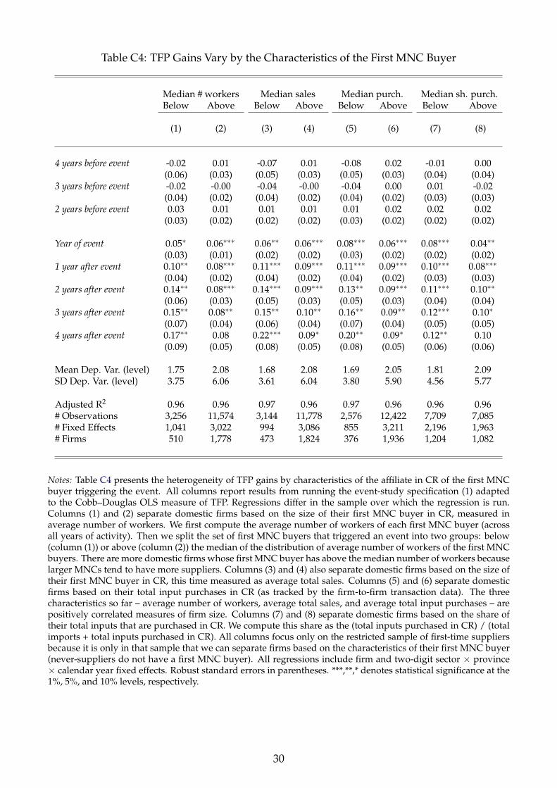
Table C4: TFP Gains Vary by the Characteristics of the First MNC Buyer

Median # workers Median sales Median purch. Median sh. purch.Below Above Below Above Below Above Below Above

(1) (2) (3) (4) (5) (6) (7) (8)

4 years before event -0.02 0.01 -0.07 0.01 -0.08 0.02 -0.01 0.00(0.06) (0.03) (0.05) (0.03) (0.05) (0.03) (0.04) (0.04)

3 years before event -0.02 -0.00 -0.04 -0.00 -0.04 0.00 0.01 -0.02(0.04) (0.02) (0.04) (0.02) (0.04) (0.02) (0.03) (0.03)

2 years before event 0.03 0.01 0.01 0.01 0.01 0.02 0.02 0.02(0.03) (0.02) (0.02) (0.02) (0.03) (0.02) (0.02) (0.02)

Year of event 0.05∗ 0.06∗∗∗ 0.06∗∗ 0.06∗∗∗ 0.08∗∗∗ 0.06∗∗∗ 0.08∗∗∗ 0.04∗∗

(0.03) (0.01) (0.02) (0.02) (0.03) (0.02) (0.02) (0.02)1 year after event 0.10∗∗ 0.08∗∗∗ 0.11∗∗∗ 0.09∗∗∗ 0.11∗∗∗ 0.09∗∗∗ 0.10∗∗∗ 0.08∗∗∗

(0.04) (0.02) (0.04) (0.02) (0.04) (0.02) (0.03) (0.03)2 years after event 0.14∗∗ 0.08∗∗∗ 0.14∗∗∗ 0.09∗∗∗ 0.13∗∗ 0.09∗∗∗ 0.11∗∗∗ 0.10∗∗

(0.06) (0.03) (0.05) (0.03) (0.05) (0.03) (0.04) (0.04)3 years after event 0.15∗∗ 0.08∗∗ 0.15∗∗ 0.10∗∗ 0.16∗∗ 0.09∗∗ 0.12∗∗∗ 0.10∗

(0.07) (0.04) (0.06) (0.04) (0.07) (0.04) (0.05) (0.05)4 years after event 0.17∗∗ 0.08 0.22∗∗∗ 0.09∗ 0.20∗∗ 0.09∗ 0.12∗∗ 0.10

(0.09) (0.05) (0.08) (0.05) (0.08) (0.05) (0.06) (0.06)

Mean Dep. Var. (level) 1.75 2.08 1.68 2.08 1.69 2.05 1.81 2.09SD Dep. Var. (level) 3.75 6.06 3.61 6.04 3.80 5.90 4.56 5.77

Adjusted R2 0.96 0.96 0.97 0.96 0.97 0.96 0.96 0.96# Observations 3,256 11,574 3,144 11,778 2,576 12,422 7,709 7,085# Fixed Effects 1,041 3,022 994 3,086 855 3,211 2,196 1,963# Firms 510 1,778 473 1,824 376 1,936 1,204 1,082

Notes: Table C4 presents the heterogeneity of TFP gains by characteristics of the affiliate in CR of the first MNCbuyer triggering the event. All columns report results from running the event-study specification (1) adaptedto the Cobb–Douglas OLS measure of TFP. Regressions differ in the sample over which the regression is run.Columns (1) and (2) separate domestic firms based on the size of their first MNC buyer in CR, measured inaverage number of workers. We first compute the average number of workers of each first MNC buyer (acrossall years of activity). Then we split the set of first MNC buyers that triggered an event into two groups: below(column (1)) or above (column (2)) the median of the distribution of average number of workers of the first MNCbuyers. There are more domestic firms whose first MNC buyer has above the median number of workers becauselarger MNCs tend to have more suppliers. Columns (3) and (4) also separate domestic firms based on the size oftheir first MNC buyer in CR, this time measured as average total sales. Columns (5) and (6) separate domesticfirms based on their total input purchases in CR (as tracked by the firm-to-firm transaction data). The threecharacteristics so far – average number of workers, average total sales, and average total input purchases – arepositively correlated measures of firm size. Columns (7) and (8) separate domestic firms based on the share oftheir total inputs that are purchased in CR. We compute this share as the (total inputs purchased in CR) / (totalimports + total inputs purchased in CR). All columns focus only on the restricted sample of first-time suppliersbecause it is only in that sample that we can separate firms based on the characteristics of their first MNC buyer(never-suppliers do not have a first MNC buyer). All regressions include firm and two-digit sector × province× calendar year fixed effects. Robust standard errors in parentheses. ***,**,* denotes statistical significance at the1%, 5%, and 10% levels, respectively.

30

Table C5: TFP Gains Vary by the HQ Country of the First MNC Buyer

Region of HQ country GDP per capita PPP Quality of managementUSA-Canada Europe Asia-Pacific LAC Below med. Above med. Below med. Above med.

(1) (2) (3) (4) (5) (6) (7) (8)

4 years before event -0.08∗∗ 0.09 0.01 0.05 -0.01 -0.02 0.06 -0.06∗

(0.04) (0.07) (0.06) (0.18) (0.05) (0.03) (0.08) (0.04)3 years before event -0.04 0.07 0.00 0.08 -0.01 -0.01 0.02 -0.03

(0.03) (0.05) (0.04) (0.11) (0.04) (0.02) (0.05) (0.03)2 years before event -0.00 0.04 0.02 0.07 0.01 0.02 0.04 0.01

(0.02) (0.03) (0.03) (0.07) (0.02) (0.02) (0.03) (0.02)

Year of event 0.09∗∗∗ 0.04 0.03 0.18∗∗ 0.03 0.08∗∗∗ 0.01 0.09∗∗∗

(0.02) (0.03) (0.03) (0.08) (0.02) (0.02) (0.03) (0.02)1 year after event 0.13∗∗∗ 0.07 0.08∗ 0.12 0.08∗∗ 0.11∗∗∗ 0.06 0.12∗∗∗

(0.03) (0.04) (0.04) (0.10) (0.04) (0.02) (0.05) (0.03)2 years after event 0.15∗∗∗ 0.06 0.09 0.07 0.10∗ 0.12∗∗∗ 0.05 0.13∗∗∗

(0.04) (0.06) (0.06) (0.14) (0.05) (0.03) (0.07) (0.03)3 years after event 0.18∗∗∗ 0.05 0.08 0.08 0.08 0.14∗∗∗ 0.04 0.15∗∗∗

(0.05) (0.08) (0.07) (0.18) (0.07) (0.04) (0.09) (0.04)4 years after event 0.19∗∗∗ 0.04 0.10 0.14 0.11 0.14∗∗∗ 0.04 0.16∗∗∗

(0.06) (0.09) (0.09) (0.21) (0.08) (0.05) (0.11) (0.05)

Mean Dep. Var. (level) 1.84 1.70 2.20 1.51 2.07 1.84 2.21 1.90SD Dep. Var. (level) 4.55 4.41 5.37 2.65 5.07 5.08 5.86 5.20

Adjusted R2 0.97 0.97 0.96 0.95 0.96 0.96 0.96 0.96# Observations 5,918 3,028 4,430 622 5,043 9,645 2,995 7,636# Fixed Effects 1,706 1,095 1,332 246 1,499 2,630 987 2,150# Firms 906 486 685 101 781 1,484 461 1,185

Notes: Table C5 presents the heterogeneity of TFP gains by characteristics of the headquarter (HQ) country of thefirst MNC buyer triggering the event. All columns report results from running the event-study specification (1)adapted to the Cobb–Douglas OLS measure of TFP. Regressions differ in the sample over which the regressionis run. Columns (1) to (4) separate domestic firms based on the region of the HQ country of the first MNCbuyer. We split countries by their geographic proximity into four groups: USA-Canada, Europe, Asia-Pacific,and Latin America and the Caribbean (LAC). Columns (5) and (6) separate domestic firms based on the GDPper capita PPP of the HQ country of the first MNC buyer. The split is with respect to the median GDP percapita across the HQ countries in our sample. The HQ countries whose GDP per capita is below median are:Nicaragua, Honduras, India, Belize, Guatemala, El Salvador, Ecuador, Indonesia, Peru, Brazil, Colombia, China,Venezuela, Serbia, Mexico, Bulgaria, Chile, Trinidad and Tobago, Greece, Panama, Hungary, Puerto Rico, andIsrael. The HQ countries whose GDP per capita is above median are: Spain, South Korea, Japan, Italy, UK,France, Canada, Australia, Belgium, Sweden, Germany, Austria, Bermuda, Netherlands, Denmark, Hong Kong,USA, Norway, Switzerland, Cayman Islands, Ireland, Singapore, and Luxembourg. Columns (7) and (8) separatedomestic firms based on the quality of management of the HQ country of the first MNC buyer. We start with thefirm-level data from the World Management Survey (WMS), which collected data for 35 countries. To computea quality management score per country, we compute a weighted average of the variable “management” (theaverage of all management questions) where the weights are the number of workers of each firm. The numberof workers comes in five categories: a) 50-100, b) 101-250, c) 251-500, d) 501-1000, and e) 1001-*. We use the lowerbound of each interval as the number of workers for the weights. Only 20 of our HQ countries are in the WMSdata. We split these countries into two groups based on whether their WMS score is above or below the medianquality of management across those 20 countries. The countries whose quality of management is below themedian are Nicaragua, India, China, Colombia, Brazil, Ireland, Greece, Spain, Chile, and Mexico. The countrieswhose quality of management is above the median are Australia, France, Italy, UK, Singapore, Sweden, Canada,Germany, Japan, and the USA. The number of observations above the median is higher because above-mediancountries have more MNCs settled in CR and more suppliers. Note that all these separations can only be donein the restricted sample, as never-suppliers do not have a first MNC buyer. Hence, all columns pertain to therestricted sample including only firms that become first-time suppliers to an MNC between 2010 and 2015. Allregressions include firm and two-digit sector × province × calendar year fixed effects. Robust standard errors inparentheses. ***,**,* denotes statistical significance at the 1%, 5%, and 10% levels, respectively.

31

Online Appendix D Robustness of Baseline Estimates

Online Appendix D.1 Robustness of Baseline Estimates to Alternative Empirical StrategiesTable D1: Baseline Event-Study Estimates Are Robust to Four Alternative Empirical Strategies

“Productive Linkages” Design Predicted Procomer Score Propensity Score Matching Nearest Neighbors Matching

Number Number Average Number Number Average Number Number Average Number Number AverageWorkers Other Corp. Corp. Sales Workers Other Corp. Corp. Sales Workers Other Corp. Corp. Sales Workers Other Corp. Corp. Sales

Buyers to Others Buyers w/ Others Buyers to Others Buyers to Others

(1) (2) (3) (4) (5) (6) (7) (8) (9) (10) (11) (12)

4 years before event 0.077 -0.036 0.017 0.100∗∗∗ -0.018 0.064 0.084∗∗∗ 0.022 0.068 -0.018 -0.012 0.006(0.161) (0.141) (0.169) (0.025) (0.038) (0.066) (0.026) (0.040) (0.062) [-0.079,0.090] [-0.138,0.170] [-0.116,0.175]

3 years before event 0.043 -0.030 0.039 0.071∗∗∗ 0.007 0.058 0.057∗∗ 0.044 0.086∗ -0.026 -0.004 0.001(0.152) (0.117) (0.178) (0.023) (0.031) (0.049) (0.024) (0.033) (0.050) [-0.069,0.056] [-0.088,0.117] [-0.103,0.100]

2 years before event -0.040 -0.039 -0.037 0.044∗∗∗ 0.012 0.047∗ 0.041∗∗ 0.037 0.051∗ -0.029 -0.014 -0.016(0.148) (0.108) (0.132) (0.016) (0.025) (0.024) (0.018) (0.029) (0.027) [-0.060,0.023] [-0.069,0.051] [-0.080,0.053]

Year of event 0.126 0.048 -0.040 0.080∗∗∗ 0.047∗∗ -0.746∗∗ 0.039∗ 0.018 -0.781∗∗∗ 0.087∗∗∗ 0.018 -1.305∗∗∗

(0.131) (0.102) (0.134) (0.016) (0.018) (0.059) (0.022) (0.022) (0.056) [0.031,0.109] [-0.053,0.064] [-1.687,-1.126]1 year after event 0.063 0.148 -0.060 0.228∗∗∗ 0.234∗∗∗ -0.055 0.108∗∗∗ 0.190∗∗∗ -0.105∗∗∗ 0.207∗∗∗ 0.271∗∗∗ -0.203∗∗∗

(0.115) (0.104) (0.128) (0.024) (0.018) (0.046) (0.022) (0.022) (0.037) [0.160,0.247] [0.191,0.324] [-0.439,-0.096]2 years after event 0.227∗ 0.254∗∗ 0.104 0.288∗∗∗ 0.297∗∗∗ 0.048 0.141∗∗∗ 0.235∗∗∗ -0.006 0.251∗∗∗ 0.353∗∗∗ -0.103∗∗

(0.118) (0.103) (0.120) (0.030) (0.028) (0.053) (0.022) (0.028) (0.049) [0.202,0.301] [0.265,0.403] [-0.345,-0.002]3 years after event 0.249∗ 0.179∗ -0.059 0.328∗∗∗ 0.340∗∗∗ 0.178∗∗ 0.161∗∗∗ 0.275∗∗∗ 0.138∗ 0.258∗∗∗ 0.398∗∗∗ -0.023

(0.130) (0.100) (0.130) (0.034) (0.026) (0.066) (0.026) (0.028) (0.072) [0.204,0.320] [0.300,0.459] [-0.190,0.087]4 years after event 0.169 0.183 -0.042 0.344∗∗∗ 0.346∗∗∗ 0.153∗∗∗ 0.173∗∗∗ 0.278∗∗∗ 0.108∗∗ 0.290∗∗∗ 0.394∗∗∗ -0.041

(0.123) (0.120) (0.121) (0.037) (0.028) (0.048) (0.030) (0.031) (0.052) [0.226,0.366] [0.277,0.471] [-0.225,0.093]

Firm FE Yes Yes Yes Yes Yes Yes Yes Yes Yes n/a n/a n/aYear FE Yes Yes Yes No No No No No No n/a n/a n/aYear-4DSect-Prov FE No No No Yes Yes Yes Yes Yes Yes n/a n/a n/a

Adjusted R2 0.88 0.91 0.57 0.79 0.87 0.63 0.78 0.88 0.63 n/a n/a n/a# Observations 1,097 1,072 1,072 107,135 71,083 71,083 98,393 70,903 70,903 91,100 72,116 72,123# Fixed Effects 123 123 123 15,470 12,540 12,540 14,888 12,275 12,275 n/a n/a n/a# Treated 31 31 31 3,606 3,383 3,383 3,599 3,380 3,380 3,670 3,252 3,254# Control 84 84 84 10,814 8,096 8,096 10,811 8,632 8,632 11,010 9,756 9,762

Notes: Table D1 contains robustness checks to the baseline results reported in Tables 1 and 2. These exercises employ the four alternative empirical strategies described in Section 3.2, each for three outcomes(all in logs): number of workers, number of other corporate buyers and average transactions with other corporate buyers (i.e., average sales to other corporate buyers). Columns (1) to (3) present the resultsfrom the “Productive Linkages” design, columns (4) to (6) those from the “predicted Procomer scores” matching, columns (7) to (9) those from the propensity score matching, and columns (10) to (12) thosefrom the nearest neighbors matching. Regressions in columns (1) to (3) include firm, deal, and year fixed effects. Regressions in columns (4) to (12) include firm and four-digit sector × province × calendaryear fixed effects. For columns (1) to (9), robust standard errors are in parentheses. For the nearest neighbors matching, 95 percent confidence intervals, given in brackets and statistical significance levels areconstructed via subsampling. ***,**,* denotes statistical significance at the 1%, 5%, and 10% levels, respectively.

32

Table D2: Auxiliary Table for the Propensity Score and Predicted Procomer Score Matching

Baseline Propensity Score Matching Predicted Procomer Score Matching

Treated Control Probit Treated Control Diff Reg Treated Control Diff(1) (2) (3) (4) (5) (6) (7) (8) (9) (10)

Agriculture, Forestry and Fishing 0.0919 0.0728 0.0736 0.0736 0 0.0736 0.0736 0(0.29) (0.26) (0.26) (0.26) (0.00) (0.26) (0.26) (0.00)

Manufacturing 0.0993 0.112 0.103 0.103 0 0.103 0.103 0(0.30) (0.32) (0.30) (0.30) (0.00) (0.30) (0.30) (0.00)

Wholesale and Retail Trade 0.363 0.318 0.320 0.320 0 0.320 0.320 0(0.48) (0.47) (0.47) (0.47) (0.00) (0.47) (0.47) (0.00)

Transportation and Storage 0.0504 0.0928 0.0945 0.0945 0 0.0945 0.0945 0(0.22) (0.29) (0.29) (0.29) (0.00) (0.29) (0.29) (0.00)

Accommodation and Food Services 0.175 0.0636 0.0648 0.0648 0 0.0648 0.0648 0(0.38) (0.24) (0.25) (0.25) (0.00) (0.25) (0.25) (0.00)

Information and Communication 0.0197 0.0360 0.0344 0.0344 0 0.0344 0.0344 0(0.14) (0.19) (0.18) (0.18) (0.00) (0.18) (0.18) (0.00)

Professional, Scientific and Technical 0.0626 0.144 0.147 0.147 0 0.147 0.147 0(0.24) (0.35) (0.35) (0.35) (0.00) (0.35) (0.35) (0.00)

Administrative and Support Services 0.0597 0.0968 0.0986 0.0986 0 0.0986 0.0986 0(0.24) (0.30) (0.30) (0.30) (0.00) (0.30) (0.30) (0.00)

Human Health and Social Work 0.0366 0.0176 0.0179 0.0179 0 0.0179 0.0179 0(0.19) (0.13) (0.13) (0.13) (0.00) (0.13) (0.13) (0.00)

Art, Entertainment and Recreation 0.0153 0.0105 0.0102 0.0102 0 0.0102 0.0102 0(0.12) (0.10) (0.10) (0.10) (0.00) (0.10) (0.10) (0.00)

Other Services 0.0253 0.0335 0.0339 0.0339 0 0.0339 0.0339 0(0.16) (0.18) (0.18) (0.18) (0.00) (0.18) (0.18) (0.00)

Mining and Quarrying 0.00109 0.00325 0.00331 0.00331 0 0.00331 0.00331 0(0.03) (0.06) (0.06) (0.06) (0.00) (0.06) (0.06) (0.00)

Located in San Jose 0.453 0.454 0.448 0.453 -0.00459 0.482 0.453 0.0296∗∗

(0.50) (0.50) (0.50) (0.50) (0.01) (0.50) (0.50) (0.01)Log Sales 5.136 5.402 0.071∗∗∗ 5.242 5.400 -0.158∗∗∗ 2.407∗∗∗ 5.223 5.400 -0.178∗∗∗

(1.05) (1.19) (0.011) (1.15) (1.18) (0.02) (0.754) (1.08) (1.18) (0.02)Log Number of Workers 1.926 1.978 -0.098∗∗∗ 1.882 1.974 -0.0924∗∗∗ 0.509 2.011 1.974 0.0368∗

(0.85) (1.04) (0.013) (0.90) (1.04) (0.02) (0.780) (0.92) (1.04) (0.02)Average Wages 14.85 14.91 0.004 14.90 14.91 0.00576 1.955 14.90 14.91 -0.00965

(0.46) (0.51) (0.020) (0.52) (0.51) (0.01) (1.330) (0.48) (0.51) (0.01)Share of College Workers 0.0620 0.0875 0.134∗∗ 0.0822 0.0875 -0.00529 0.971 0.0707 0.0875 -0.0168∗∗∗

(0.13) (0.18) (0.058) (0.18) (0.18) (0.00) (3.186) (0.16) (0.18) (0.00)Workers w/ Exp. at Supp. of MNCs 0.413 0.666 0.213∗∗∗ 0.660 0.666 0.00597 -1.386 0.504 0.666 -0.161∗∗∗

(0.49) (0.47) (0.021) (0.47) (0.47) (0.01) (1.668) (0.50) (0.47) (0.01)Workers w/ Exp. at MNCs 0.439 0.582 0.084∗∗∗ 0.575 0.582 0.00689∗ 1.021 0.508 0.582 -0.0744∗∗∗

(0.50) (0.49) (0.019) (0.49) (0.49) (0.01) (1.570) (0.50) (0.49) (0.01)Year of Firm Entry 2007.7 2009.4 0.100∗∗∗ 2009.4 2009.5 0.503∗∗ 0.664∗∗∗ 2008.0 2009.5 -1.415∗∗∗

(3.26) (3.39) (0.003) (3.14) (3.39) (0.06) (0.254) (3.08) (3.39) (0.06)Exporter 0.0231 0.0622 0.045 0.0417 0.0579 -0.0162∗∗∗ 0.472 0.0337 0.0579 -0.0242∗∗∗

(0.15) (0.24) (0.039) (0.20) (0.23) (0.00) (1.481) (0.18) (0.23) (0.00)Importer 0.159 0.288 0.180∗∗∗ 0.235 0.284 -0.0497∗∗∗ 2.019 0.191 0.284 -0.0937∗∗∗

(0.37) (0.45) (0.022) (0.42) (0.45) (0.01) (1.518) (0.18) (0.23) (0.00)Supplies to a Big Domestic Firm 0.0811 0.317 0.239∗∗∗ 0.213 0.315 -0.103∗∗∗ -3.388∗ 0.0966 0.315 -0.219∗∗∗

(0.27) (0.47) (0.022) (0.41) (0.46) (0.01) (1.943) (0.30) (0.46) (0.01)Supplies to an Exporter 0.0389 0.182 0.145∗∗∗ 0.0969 0.181 -0.0841∗∗∗ -3.190∗ 0.0429 0.181 -0.138∗∗∗

(0.19) (0.39) (0.026) (0.30) (0.39) (0.01) (1.885) (0.20) (0.39) (0.00)Number of Suppliers 2.889 3.988 0.009∗∗∗ 3.217 3.984 -0.767∗∗∗ -0.052 2.761 3.984 -1.223∗∗∗

(5.41) (7.37) (0.001) (6.17) (7.35) (0.12) (0.049) (5.55) (7.35) (0.12)Number of Buyers 3.954 12.38 0.001∗∗ 6.917 12.39 -5.477∗∗∗ -0.003 5.186 12.39 -7.209∗∗∗

(16.67) (32.30) (0.000) (21.10) (32.52) (0.47) (0.018) (17.68) (32.52) (0.43)Av. Duration w/ Buyers (Years) 1.157 1.436 0.037∗∗∗ 1.297 1.421 -0.124∗∗∗ 0.260 1.359 1.421 -0.0617∗∗∗

(1.81) (1.05) (0.008) (1.28) (0.68) (0.02) (0.699) (1.51) (0.68) (0.03)Procomer Score 72.09 72.28 -0.0185∗

(3.67) (4.04) (0.07)

# Controls 14,338 14,338 10,887 10,887 10,887 10,887 10,887 10,887# Treated 3,697 3,697 3,629 3,629 3,629 3,629 3,629 3,629# Observations in Regression 119,552 630

Notes: Table D2 presents the auxiliary regressions (columns (3) and (7)) and the comparisons between treated and control firms for thepropensity score matching (PSM, columns (4) to (6)) and predicted Procomer scores matching (columns (8) to (10)). All descriptive statisticspertain to the year of the event. For reference, columns (1) and (2) present the averages for the baseline economy-wide full sample, includingboth domestic firms that become first-time suppliers to an MNC and domestic firms never observed as supplying to an MNC in our sampleperiod. Column (3) presents the coefficients from the probit model where the outcome variable is the conditional probability of being chosenas a first-time supplier to an MNC in a given year. All the firm-specific controls are contemporaneous. The probit specification also controlsfor four-digit sector, year and province FEs. Columns (4), (5), and (6) compare the treated and control samples for the PSM specification.Column (7) presents the coefficients from a regression of the Procomer scores on a set of firm characteristics (all contemporaneous). Thisregression also controls for twenty broad-sector FEs. We then use the estimated coefficients to predict Procomer scores for all firm-years inthe economy-wide sample. Columns (8), (9), and (10) compare the treated and control samples for the Predicted Procomer scores specification.***,**,* denotes statistical significance at the 1%, 5%, and 10% levels, respectively.

33

Table D3: “Productive Linkages” Design: Event Study Patterns for “Losers”

Total Number TFP Corp. Number Av. SalesSales Workers CD OLS Sales Other Other

Others Buyers Buyers(1) (2) (3) (4) (5) (6)

4 years before event -0.199 -0.145 0.019 0.053 -0.204 0.257(0.277) (0.204) (0.112) (0.264) (0.152) (0.157)

3 years before event -0.119 -0.100 0.037 0.033 -0.138 0.171(0.205) (0.151) (0.084) (0.194) (0.109) (0.125)

2 years before event -0.048 -0.074 0.017 0.041 -0.056 0.096(0.133) (0.102) (0.064) (0.135) (0.080) (0.090)

Year of event -0.010 -0.040 -0.022 -0.200 0.005 -0.206∗∗

(0.123) (0.103) (0.060) (0.134) (0.077) (0.086)1 year after event -0.038 -0.038 -0.030 -0.038 0.075 -0.113

(0.179) (0.127) (0.080) (0.176) (0.096) (0.115)2 years after event -0.101 -0.116 -0.045 -0.233 0.060 -0.293∗

(0.250) (0.183) (0.107) (0.259) (0.136) (0.167)3 years after event 0.018 -0.137 -0.006 -0.180 0.120 -0.300

(0.323) (0.238) (0.136) (0.326) (0.170) (0.210)4 years after event 0.041 -0.074 -0.005 -0.228 0.159 -0.387

(0.386) (0.286) (0.165) (0.388) (0.205) (0.246)

Adjusted R2 0.83 0.88 0.96 0.81 0.91 0.56# Observations 1,111 1,097 1,087 1,072 1,072 1,072# Treated 31 31 31 31 31 31# Control 84 84 84 84 84 84

Notes: Table D3 contains a robustness check to the baseline event-study results presented in Tables 1 and 2. Thistable focuses on the “Productive Linkages” research design. We show the findings for six dependent variables:log total sales, log number of workers, log TFP residual from an OLS regression that assumes a Cobb–Douglastechnology, log corporate sales to others, log number of other corporate buyers, and log average sales to othercorporate buyers. The six columns report the estimates for the θL

k coefficients (see equation (2)). These coefficientsmeasure the effects of the event on the outcomes of the “losers” to a given deal (i.e., the other firms shortlistedfor a deal through “Productive Linkages”). Robust standard errors in parentheses. ***,**,* denotes statisticalsignificance at the 1%, 5%, and 10% levels, respectively.

34

Online Appendix D.1.1 More Details on Nearest Neighbors Matching

Denote the outcome of the first-time supplier i at event-time k as Yi,k. Let Yi,k(1) = Yi,k bethe observable outcome of firm i at event-time k when treated and Yi,k(0) be the counterfactualoutcome corresponding to the same event-time k but in the absence of the event.xvii We usethe control firms to create an estimate of Yi,k(0). Let Jn(i) be the set of the n nearest neighborsof firm i. We denote Yi,k(0) as:

Yi,k(0) =1n ∑

j∈Jn(i)Yj,k(0),

where Yj,k(0) is the observed outcome of firm j corresponding to event-time k associated withfirm i. We compute the difference in difference estimate βi,k by netting out the average differ-ence between treated and control firms in the year prior to the event. This means that:

βi,k = Yi,k(1)− Yi,k(0)− (Yi,−1(1)− Yi,−1(0))

Let N1 be the total number of treated firms. The average impact at event-time k is just themean of the firm-specific treatment effects:

βk =1

N1

N

∑i=1

βi,k

We implement a subsampling procedure to construct confidence intervals.xviii In par-ticular we use Nb = 500 subsamples. For each subsample, we select without replacementB1 = R

√N1 treated firms and B0 = R(N0/

√N1) control firms, where N0 is the total number

of potential control firms and R is a turning parameter (Politis and Romano, 1994; Deryuginaet al., 2020).xix The estimated CDF of βk is given by:

F(x) =1

Nb

Nb

∑b=1

1[√

B1√N1

(βbk − βk) + βk < x]

The confidence interval is then: [F−1(0.025), F−1(0.975)].For more details, see Abadie and Imbens (2006) for the theory and Deryugina et al. (2020)

for an application.

xviiFor each year, we standardize the outcome variables by computing a z-score. We first subtract the yearly averageand then divide by the standard deviation (both across all firms in the economy that year).

xviiiWe use subsampling as opposed to bootstrap since the bootstrap fails for nearest neighbor matching due to thenon-smoothness of the nearest neighbor function. However, the subsampling methods in Politis and Romano(1994) remains as a valid inferential method (Abadie and Imbens, 2008).

xixWe use R = 3 as in Deryugina et al. (2020). However, results are also similar for R = 5 and R = 10.

35

Online Appendix D.2 Robustness of Baseline Estimates to Alternative

Control Groups

Table D4: Robustness of Baseline Estimates to Dropping All Never-Supplying Firms from theControl Group

Firm Size TFP Business with Others

Total Number Input CD ACF Sales to Corp. Sales Number Other Average Corp.Sales Workers Costs OLS (2015) to Others to Others Corp. Buyers Sales to Others

(1) (2) (3) (4) (5) (6) (7) (8) (9)

4 years before event -0.022 -0.054 0.003 -0.012 0.027 -0.047 -0.139 -0.042 -0.096(0.053) (0.049) (0.069) (0.022) (0.020) (0.119) (0.148) (0.048) (0.137)

3 years before event 0.001 -0.027 0.057 -0.004 0.032∗ -0.041 -0.103 -0.014 -0.088(0.041) (0.035) (0.049) (0.015) (0.016) (0.076) (0.100) (0.033) (0.094)

2 years before event 0.007 -0.010 0.036 0.010 0.013 -0.028 -0.029 0.002 -0.031(0.023) (0.019) (0.030) (0.013) (0.011) (0.036) (0.045) (0.022) (0.048)

Year of event 0.191∗∗∗ 0.088∗∗∗ 0.110∗∗∗ 0.061∗∗∗ 0.043∗∗∗ -0.122∗ -0.636∗∗∗ 0.031 -0.667∗∗∗

(0.021) (0.019) (0.026) (0.009) (0.008) (0.062) (0.074) (0.022) (0.071)1 year after event 0.377∗∗∗ 0.286∗∗∗ 0.252∗∗∗ 0.090∗∗∗ 0.053∗∗∗ 0.205∗∗ 0.295∗∗∗ 0.226∗∗∗ 0.069

(0.035) (0.031) (0.044) (0.013) (0.013) (0.090) (0.095) (0.034) (0.089)2 years after event 0.408∗∗∗ 0.317∗∗∗ 0.255∗∗∗ 0.097∗∗∗ 0.050∗∗∗ 0.320∗∗∗ 0.484∗∗∗ 0.282∗∗∗ 0.202∗

(0.054) (0.046) (0.072) (0.017) (0.017) (0.115) (0.121) (0.047) (0.112)3 years after event 0.389∗∗∗ 0.313∗∗∗ 0.241∗∗ 0.101∗∗∗ 0.041∗ 0.333∗∗ 0.683∗∗∗ 0.312∗∗∗ 0.370∗∗

(0.072) (0.061) (0.095) (0.021) (0.021) (0.147) (0.164) (0.061) (0.161)4 years after event 0.382∗∗∗ 0.295∗∗∗ 0.252∗∗ 0.099∗∗∗ 0.036 0.380∗∗ 0.704∗∗∗ 0.321∗∗∗ 0.383∗

(0.089) (0.074) (0.115) (0.027) (0.027) (0.171) (0.201) (0.073) (0.191)

Firm FE Yes Yes Yes Yes Yes Yes Yes Yes YesYear-4DSect-Prov FE Yes Yes Yes Yes Yes Yes Yes Yes Yes

Mean Dep. Var. (level) 1.45 18.9 1.40 2.00 -0.00 1.42 0.56 19.1 0.033SD Dep. Var. (level) 4.50 45.1 4.74 5.74 0.34 4.51 1.81 57.7 0.045

Adjusted R2 0.80 0.77 0.86 0.96 0.64 0.64 0.59 0.84 0.51# Observations 23,961 23,961 14,199 13,706 13,706 23,801 20,491 20,491 20,491# Fixed Effects 7,366 7,366 4,870 4,774 4,774 7,328 6,742 6,742 6,742# Firms 3,482 3,482 2,195 2,144 2,144 3,468 3,291 3,291 3,291

Notes: Table D4 shows the results of running the event-study specification (1) for nine of our most importantoutcome variables. These results differ from those in Tables 1 and 2 in the sample of firms allowed in the controlgroup. All columns report event-study estimates for the restricted sample of domestic firms becoming first-timesuppliers to an MNC between 2010 and 2015 (i.e., the baseline sample from which we have excluded all never-suppliers to an MNC). The first three outcome variables are measures of firm size: log total sales (column (1)),log number of workers (column (2)) and log input costs (as a proxy for materials, column (3)). Columns (4) and(5) consider two measures of TFP. Column (4) uses a measure of TFP resulting from OLS production functionestimation and assumes a Cobb–Douglas technology, with revenues (CPI-deflated to 2013 U.S. dollars) as theoutput measure and total net assets, number of workers, and input costs as input measures for K, L, and Mrespectively. Column (5) shows the results of production function estimation following Ackerberg et al. (2015).Columns (6) to (9) study the performance of firms in their business with other buyers. Column (6) studies thelog sales to others (sales to all buyers except the first MNC buyer). Column (7) studies the log transactions toothers (sales to all corporate buyers except the first MNC buyer). Column (8) studies the log number of othercorporate buyers + 1 (number of corporate buyers tracked by the firm-to-firm transaction data, except the firstMNC buyer, + 1). Finally, column (9) studies the log average sales to other corporate buyers (total sales to othercorporate buyers, divided by the number of other corporate buyers, except the first MNC buyer, +1). All columnsuse standard error clustering at event-by-province level. Event year clustering is recommended whenever eventdates are concentrated on a few values, as in our case from 2010 to 2015. Except for the number of workers and thenumber of buyers, means (in levels) are reported in millions of U.S. dollars (CPI-deflated to 2013 dollars). Robuststandard errors in parentheses. ***,**,* denotes statistical significance at the 1%, 5%, and 10% levels, respectively.

36

Table D5: Robustness of Baseline Estimates to Restricting the Control Group to Only IncludeSuppliers to Large Firms

Firm Size TFP Business with Others

Total Number Input CD ACF Sales to Corp. Sales Number Other Average Corp.Sales Workers Costs OLS (2015) to Others to Others Corp. Buyers Sales to Others

(1) (2) (3) (4) (5) (6) (7) (8) (9)

4 years before event 0.021 0.003 -0.001 0.008 0.012 0.007 0.058 -0.023 0.081(0.041) (0.033) (0.058) (0.017) (0.015) (0.055) (0.086) (0.035) (0.061)

3 years before event 0.016 -0.004 0.049 0.014 0.022∗ -0.019 0.027 -0.006 0.033(0.029) (0.022) (0.038) (0.013) (0.013) (0.041) (0.053) (0.027) (0.042)

2 years before event 0.018 0.006 0.028 0.012 0.006 -0.018 0.037 0.004 0.033(0.023) (0.014) (0.025) (0.011) (0.010) (0.034) (0.033) (0.018) (0.027)

Year of event 0.168∗∗∗ 0.064∗∗∗ 0.097∗∗∗ 0.058∗∗∗ 0.045∗∗∗ -0.165∗∗∗ -0.701∗∗∗ 0.027∗ -0.728∗∗∗

(0.021) (0.024) (0.027) (0.010) (0.008) (0.051) (0.092) (0.016) (0.082)1 year after event 0.343∗∗∗ 0.244∗∗∗ 0.228∗∗∗ 0.087∗∗∗ 0.061∗∗∗ 0.138∗∗ 0.154∗∗ 0.219∗∗∗ -0.065

(0.033) (0.032) (0.031) (0.015) (0.011) (0.058) (0.066) (0.018) (0.058)2 years after event 0.369∗∗∗ 0.266∗∗∗ 0.231∗∗∗ 0.095∗∗∗ 0.069∗∗∗ 0.231∗∗∗ 0.277∗∗∗ 0.269∗∗∗ 0.009

(0.035) (0.035) (0.041) (0.013) (0.011) (0.048) (0.076) (0.022) (0.068)3 years after event 0.346∗∗∗ 0.251∗∗∗ 0.210∗∗∗ 0.097∗∗∗ 0.065∗∗∗ 0.211∗∗∗ 0.404∗∗∗ 0.292∗∗∗ 0.112∗

(0.038) (0.037) (0.053) (0.016) (0.012) (0.049) (0.071) (0.026) (0.062)4 years after event 0.342∗∗∗ 0.224∗∗∗ 0.230∗∗∗ 0.094∗∗∗ 0.066∗∗∗ 0.237∗∗∗ 0.358∗∗∗ 0.291∗∗∗ 0.067

(0.040) (0.036) (0.059) (0.017) (0.015) (0.049) (0.070) (0.031) (0.060)

Firm FE Yes Yes Yes Yes Yes Yes Yes Yes YesYear-4DSect-Prov FE Yes Yes Yes Yes Yes Yes Yes Yes Yes

Mean Dep. Var. (level) 1.29 16.4 1.22 1.68 -0.00 1.27 0.50 17.5 0.035SD Dep. Var. (level) 3.74 37.7 3.97 4.59 0.35 3.74 1.52 48.9 0.048

Adjusted R2 0.79 0.75 0.84 0.96 0.62 0.67 0.61 0.84 0.54# Observations 40,539 40,539 25,826 24,930 24,930 40,382 34,318 34,318 34,318# Fixed Effects 10,807 10,807 7,507 7,348 7,348 10,774 9,921 9,921 9,921# Firms 5,754 5,754 3,866 3,771 3,771 5,742 5,395 5,395 5,395

Notes: Table D5 shows the results of running the event-study specification (1) for nine of our most importantoutcome variables. These results differ from those in Tables 1 and 2 in the sample of firms allowed in the controlgroup. Namely, all columns correspond to a sample including only the first-time suppliers to MNCs and firmsthat are never-suppliers to MNCs but that supply to at least one big domestic firm sometime between 2008 and2017. Put differently, this sample starts from the baseline sample from which we exclude firms that were bothnever-suppliers to an MNC and never-suppliers to a large domestic firm. We define large domestic firms asdomestic firms whose median number of workers across all years of activity is larger than 100. The first threeoutcome variables are measures of firm size: log total sales (column (1)), log number of workers (column (2))and log input costs (as a proxy for materials, column (3)). Columns (4) and (5) consider two measures of TFP.Column (4) uses a measure of TFP resulting from OLS production function estimation and assumes a Cobb–Douglas technology, with revenues (CPI-deflated to 2013 U.S. dollars) as the output measure and total net assets,number of workers, and input costs as input measures for K, L, and M respectively. Column (5) shows the resultsof production function estimation following Ackerberg et al. (2015). Columns (6) to (9) study the performanceof firms in their business with other buyers. Column (6) studies the log sales to others (sales to all buyers exceptthe first MNC buyer). Column (7) studies the log transactions to others (sales to all corporate buyers except thefirst MNC buyer). Column (8) studies the log number of other corporate buyers + 1 (number of corporate buyerstracked by the firm-to-firm transaction data, except the first MNC buyer, + 1). Finally, column (9) studies the logaverage sales to other corporate buyers (total sales to other corporate buyers, divided by the number of othercorporate buyers, except the first MNC buyer, +1). Except for the number of workers and the number of buyers,means (in levels) are reported in millions of U.S. dollars (CPI-deflated to 2013 dollars). Robust standard errors inparentheses. ***,**,* denotes statistical significance at the 1%, 5%, and 10% levels, respectively.

37

Online Appendix D.3 Robustness of Baseline Estimates to Excluding First-time Suppliers Hiring New Man-

agers or Former Workers for an MNC or for a Supplier to an MNC

Table D6: Robustness of Baseline Estimates to Excluding First-time Suppliers Hiring New Managers or Former Workers for an MNC or aSupplier to an MNC

Baseline No ∆ Top 1 No ∆ Top 2 No ∆ Top 1 No ∆ Top 2 No Occ Mng No Occ Mng No MNC Emp No MNC Emp No Supp Emp No Supp EmpEvent Event Event-1 Event-1 Event Event-1 Event Event-1 Event Event-1

(1) (2) (3) (4) (5) (6) (7) (8) (9) (10) (11)

4 years before event 0.016 0.019 0.016 0.016 0.015 0.014 0.016 0.013 0.019 0.008 0.023(0.014) (0.016) (0.014) (0.015) (0.014) (0.014) (0.015) (0.019) (0.023) (0.017) (0.018)

3 years before event 0.020∗∗ 0.020∗∗ 0.015 0.018∗ 0.021∗∗ 0.018 0.027∗∗ 0.016 0.012 0.023∗∗ 0.023∗

(0.010) (0.010) (0.010) (0.010) (0.010) (0.011) (0.011) (0.013) (0.015) (0.011) (0.012)2 years before event 0.015 0.016 0.009 0.016 0.018∗ 0.016 0.020∗∗ 0.033∗∗∗ 0.021∗ 0.024∗∗ 0.016

(0.010) (0.010) (0.011) (0.011) (0.010) (0.010) (0.010) (0.010) (0.012) (0.010) (0.011)

Year of event 0.059∗∗∗ 0.054∗∗∗ 0.050∗∗∗ 0.056∗∗∗ 0.054∗∗∗ 0.063∗∗∗ 0.062∗∗∗ 0.070∗∗∗ 0.049∗∗∗ 0.058∗∗∗ 0.055∗∗∗

(0.009) (0.009) (0.009) (0.009) (0.009) (0.010) (0.010) (0.011) (0.012) (0.009) (0.010)1 year after event 0.082∗∗∗ 0.080∗∗∗ 0.079∗∗∗ 0.080∗∗∗ 0.074∗∗∗ 0.083∗∗∗ 0.085∗∗∗ 0.079∗∗∗ 0.069∗∗∗ 0.079∗∗∗ 0.080∗∗∗

(0.014) (0.014) (0.014) (0.014) (0.013) (0.015) (0.015) (0.013) (0.019) (0.012) (0.015)2 years after event 0.088∗∗∗ 0.085∗∗∗ 0.081∗∗∗ 0.085∗∗∗ 0.083∗∗∗ 0.089∗∗∗ 0.093∗∗∗ 0.091∗∗∗ 0.079∗∗∗ 0.090∗∗∗ 0.088∗∗∗

(0.011) (0.012) (0.011) (0.011) (0.011) (0.012) (0.012) (0.014) (0.015) (0.011) (0.012)3 years after event 0.088∗∗∗ 0.084∗∗∗ 0.086∗∗∗ 0.084∗∗∗ 0.083∗∗∗ 0.088∗∗∗ 0.093∗∗∗ 0.093∗∗∗ 0.078∗∗∗ 0.089∗∗∗ 0.089∗∗∗

(0.014) (0.014) (0.014) (0.014) (0.014) (0.014) (0.015) (0.018) (0.016) (0.014) (0.014)4 years after event 0.086∗∗∗ 0.085∗∗∗ 0.084∗∗∗ 0.085∗∗∗ 0.080∗∗∗ 0.087∗∗∗ 0.091∗∗∗ 0.089∗∗∗ 0.076∗∗∗ 0.089∗∗∗ 0.088∗∗∗

(0.015) (0.015) (0.015) (0.015) (0.015) (0.016) (0.016) (0.018) (0.021) (0.014) (0.016)

Adjusted R2 0.95 0.95 0.95 0.95 0.95 0.95 0.95 0.94 0.94 0.95 0.95# Observations 64,419 63,338 62,649 63,619 63,191 63,484 63,798 58,723 59,759 61,911 63,171# Fixed Effects 15,464 15,202 15,035 15,283 15,223 15,257 15,329 14,196 14,504 14,900 15,220# Firms 10,492 10,292 10,165 10,371 10,297 10,357 10,412 9,621 9,851 10,072 10,309

Notes: Table D6 explores the robustness of the baseline estimates to excluding first-time suppliers having hired workers that could bring about both a first linkage toan MNC and improvements in firm performance. We focus on the TFP residual from an OLS regression that assumes a Cobb–Douglas technology. Column (1) reportsour baseline estimates. Columns (2) to (5) exclude first-time suppliers having hired new managers either in the event year (“Event”) or in the year before the event(“Event-1”). We identify managers as the top earners. Columns (2) and (4) exclude first-time suppliers having hired a new worker who became the top earner in thefirm, whereas columns (3) and (5) also exclude first-time suppliers having hired a new worker who became the top two earner in the firm. Columns (6) and (7) identifymanagers based on their occupation code (major category 1 in the ISCO-08 classification). We only drop firms whose new managers are new hires. Columns (8) and(9) exclude first-time suppliers having hired a new worker whose main employer in the previous year was one of the 622 MNC affiliates in CR (irrespective of theoccupation that this new worker holds at the new firm). Columns (10) and (11) exclude first-time suppliers having hired a new worker whose main employer in theprevious year had supplied to any of the 622 MNCs at any time before the year when the employee moved to the first-time supplier. All columns correspond to the fulleconomy-wide sample (including first-time suppliers to MNCs and never-suppliers). ***,**,* denotes statistical significance at the 1%, 5%, and 10% levels, respectively.

38

Online Appendix D.4 Robustness of Baseline Estimates to Different Sam-

ple Selection Criteria

Table D7: Robustness of Baseline Estimates to Sample Restrictions: No Size Restrictions forDomestic Firms; No Sector Restrictions for Domestic Firms

No size restrictions for domestic firms No sector restrictions for domestic firms

Total Number TFP Corp. Number Av. Sales Total Number TFP Corp. Number Av. SalesSales Workers CD OLS Sales Other Other Sales Workers CD OLS Sales Other Other

Others Buyers Buyers Others Buyers Buyers(1) (2) (3) (4) (5) (6) (7) (8) (9) (10) (11) (12)

4 years before event 0.01 -0.04∗ 0.03 0.02 -0.04 0.05 0.05∗ -0.01 0.02 -0.02 -0.01 -0.02(0.02) (0.02) (0.02) (0.07) (0.03) (0.05) (0.03) (0.02) (0.02) (0.08) (0.03) (0.06)

3 years before event 0.02 -0.02 0.02 0.02 -0.01 0.03 0.03 -0.01 0.02∗ 0.00 0.01 -0.01(0.02) (0.02) (0.01) (0.04) (0.02) (0.04) (0.02) (0.02) (0.01) (0.04) (0.02) (0.04)

2 years before event 0.03 -0.00 0.02 -0.01 -0.00 -0.01 0.02 -0.01 0.02∗∗ 0.02 0.01 0.01(0.02) (0.01) (0.01) (0.03) (0.01) (0.03) (0.02) (0.01) (0.01) (0.03) (0.01) (0.03)

Year of event 0.18∗∗∗ 0.05∗∗∗ 0.07∗∗∗ -0.98∗∗∗ 0.02 -1.00∗∗∗ 0.16∗∗∗ 0.05∗∗ 0.06∗∗∗ -0.87∗∗∗ 0.02 -0.89∗∗∗

(0.02) (0.02) (0.01) (0.09) (0.01) (0.08) (0.02) (0.02) (0.01) (0.10) (0.02) (0.09)1 year after event 0.30∗∗∗ 0.19∗∗∗ 0.09∗∗∗ -0.02 0.19∗∗∗ -0.21∗∗∗ 0.31∗∗∗ 0.22∗∗∗ 0.08∗∗∗ 0.12∗∗ 0.21∗∗∗ -0.09∗∗

(0.02) (0.02) (0.01) (0.07) (0.02) (0.06) (0.03) (0.03) (0.01) (0.05) (0.02) (0.04)2 years after event 0.31∗∗∗ 0.22∗∗∗ 0.09∗∗∗ 0.20∗∗∗ 0.24∗∗∗ -0.03 0.33∗∗∗ 0.24∗∗∗ 0.08∗∗∗ 0.27∗∗∗ 0.26∗∗∗ 0.01

(0.03) (0.02) (0.01) (0.07) (0.02) (0.06) (0.03) (0.03) (0.02) (0.06) (0.02) (0.05)3 years after event 0.30∗∗∗ 0.22∗∗∗ 0.08∗∗∗ 0.35∗∗∗ 0.26∗∗∗ 0.09 0.32∗∗∗ 0.24∗∗∗ 0.08∗∗∗ 0.42∗∗∗ 0.28∗∗∗ 0.14∗∗∗

(0.03) (0.02) (0.01) (0.07) (0.02) (0.06) (0.03) (0.03) (0.02) (0.06) (0.02) (0.05)4 years after event 0.30∗∗∗ 0.22∗∗∗ 0.08∗∗∗ 0.43∗∗∗ 0.28∗∗∗ 0.15∗∗ 0.32∗∗∗ 0.23∗∗∗ 0.08∗∗∗ 0.43∗∗∗ 0.29∗∗∗ 0.14∗∗∗

(0.03) (0.02) (0.01) (0.07) (0.02) (0.06) (0.03) (0.03) (0.02) (0.06) (0.03) (0.05)

Mean Dep. Var. (level) 0.49 7.76 0.74 0.25 9.17 0.031 0.90 16.9 1.19 0.37 13.0 0.041SD Dep. Var. (level) 1.81 22.8 2.48 0.92 29.5 0.048 2.76 117.3 3.43 1.08 49.2 0.059

Firm FE Yes Yes Yes Yes Yes Yes Yes Yes Yes Yes Yes YesYear-4DSect-Prov FE Yes Yes Yes Yes Yes Yes Yes Yes Yes Yes Yes YesNever Suppliers Yes Yes Yes Yes Yes Yes Yes Yes Yes Yes Yes Yes

Adjusted R2 0.84 0.80 0.95 0.64 0.84 0.58 0.76 0.75 0.95 0.62 0.83 0.57# Observations 244,488 244,488 111,812 112,870 112,870 112,870 136,011 136,011 68,012 72,229 72,229 72,229# Fixed Effects 53,229 53,229 27,378 29,537 29,537 29,537 29,466 29,466 16,670 19,142 19,142 19,142# Firms 44,223 44,223 21,022 22,288 22,288 22,288 21,310 21,310 11,271 12,695 12,695 12,695

Notes: Table D7 shows the results of running the event-study specification (1) for six of our most importantoutcome variables. The main difference between the two samples in this table and the baseline sample describedin Section 2.2 and used in Tables 1 and 2 comes from the restrictions used in the sample creation. The sample incolumns (1) to (6) relaxes the size restrictions for domestic firms used in the baseline sample (while still keepingin place the sector restrictions for domestic firms and the 100-worker restriction on the size of MNCs triggeringthe first-time supplying events). The sample in columns (7) to (12) relaxes the sector restrictions for domesticfirms used in the baseline sample (while still keeping in place the size restrictions for domestic firms and the100-worker restriction on the size of MNCs triggering the first-time supplying events). All columns correspondto the full sample including both first-time suppliers and never-suppliers. Except for the number of workersand the number of other buyers, means (in levels) are reported in millions of U.S. dollars (CPI-deflated to 2013dollars). Robust standard errors in parentheses. ***,**,* denotes statistical significance at the 1%, 5%, and 10%levels, respectively.

39

Table D8: Robustness of Baseline Estimates to Sample Restrictions: No Size and Sector Restric-tions for Domestic Firms; + All “MNCs”

No size and sector restrictions for domestic firms No size and sector restrictions for domestic firms, all “MNCs”

Total Number TFP Corp. Number Av. Sales Total Number TFP Corp. Number Av. SalesSales Workers CD OLS Sales Other Other Sales Workers CD OLS Sales Other Other

Others Buyers Buyers Others Buyers Buyers(1) (2) (3) (4) (5) (6) (7) (8) (9) (10) (11) (12)

4 years before event 0.02 -0.04∗∗ 0.03∗ -0.00 -0.03 0.03 0.04∗ -0.03∗∗ 0.03∗ 0.02 -0.04∗ 0.06(0.02) (0.02) (0.02) (0.06) (0.02) (0.05) (0.02) (0.02) (0.01) (0.06) (0.02) (0.05)

3 years before event 0.03 -0.02 0.02 0.02 -0.00 0.02 0.04∗∗ -0.01 0.02 0.09∗∗ 0.01 0.08∗∗

(0.02) (0.01) (0.01) (0.04) (0.01) (0.04) (0.02) (0.01) (0.01) (0.04) (0.01) (0.04)2 years before event 0.02 -0.02 0.02∗∗ -0.00 -0.00 0.00 0.02∗ -0.01 0.02∗∗ 0.01 -0.01 0.02

(0.02) (0.01) (0.01) (0.03) (0.01) (0.03) (0.01) (0.01) (0.01) (0.03) (0.01) (0.03)

Year of event 0.18∗∗∗ 0.04∗∗∗ 0.07∗∗∗ -1.09∗∗∗ 0.01 -1.10∗∗∗ 0.18∗∗∗ 0.05∗∗∗ 0.07∗∗∗ -1.32∗∗∗ -0.01 -1.31∗∗∗

(0.02) (0.02) (0.01) (0.09) (0.01) (0.08) (0.02) (0.02) (0.01) (0.09) (0.01) (0.09)1 year after event 0.29∗∗∗ 0.18∗∗∗ 0.08∗∗∗ -0.04 0.17∗∗∗ -0.22∗∗∗ 0.30∗∗∗ 0.18∗∗∗ 0.08∗∗∗ -0.08 0.18∗∗∗ -0.26∗∗∗

(0.02) (0.02) (0.01) (0.06) (0.02) (0.05) (0.02) (0.02) (0.01) (0.06) (0.02) (0.05)2 years after event 0.29∗∗∗ 0.20∗∗∗ 0.08∗∗∗ 0.19∗∗∗ 0.22∗∗∗ -0.04 0.31∗∗∗ 0.20∗∗∗ 0.08∗∗∗ 0.20∗∗∗ 0.24∗∗∗ -0.05

(0.03) (0.02) (0.01) (0.06) (0.02) (0.05) (0.02) (0.02) (0.01) (0.06) (0.02) (0.05)3 years after event 0.29∗∗∗ 0.20∗∗∗ 0.07∗∗∗ 0.32∗∗∗ 0.25∗∗∗ 0.08 0.30∗∗∗ 0.20∗∗∗ 0.08∗∗∗ 0.35∗∗∗ 0.26∗∗∗ 0.09∗

(0.03) (0.02) (0.01) (0.06) (0.02) (0.05) (0.03) (0.02) (0.01) (0.06) (0.02) (0.05)4 years after event 0.29∗∗∗ 0.20∗∗∗ 0.07∗∗∗ 0.43∗∗∗ 0.27∗∗∗ 0.15∗∗∗ 0.29∗∗∗ 0.20∗∗∗ 0.08∗∗∗ 0.45∗∗∗ 0.29∗∗∗ 0.16∗∗∗

(0.03) (0.02) (0.01) (0.06) (0.02) (0.05) (0.03) (0.02) (0.01) (0.06) (0.02) (0.05)

Mean Dep. Var. (level) 0.51 9.59 0.79 0.25 9.23 0.032 0.49 9.35 0.75 0.24 8.88 0.032SD Dep. Var. (level) 1.98 81.6 2.70 0.84 37.3 0.050 1.89 82.4 2.56 0.83 37.3 0.050

Firm FE Yes Yes Yes Yes Yes Yes Yes Yes Yes Yes Yes YesYear-4DSect-Prov FE Yes Yes Yes Yes Yes Yes Yes Yes Yes Yes Yes YesNever Suppliers Yes Yes Yes Yes Yes Yes Yes Yes Yes Yes Yes Yes

Adjusted R2 0.84 0.81 0.95 0.63 0.83 0.58 0.84 0.81 0.95 0.61 0.82 0.57# Observations 283,436 283,436 117,309 130,096 130,096 130,096 275,568 275,568 113,200 122,916 122,916 122,916# Fixed Effects 62,255 62,255 29,310 34,069 34,069 34,069 61,005 61,005 28,537 32,759 32,759 32,759# Firms 51,975 51,975 22,409 25,996 25,996 25,996 50,807 50,807 21,757 24,837 24,837 24,837

Notes: Table D8 shows the results of running the event-study specification (1) for six of our most importantoutcome variables. The main difference between the samples in this table and the baseline sample describedin Section 2.2 and used in Tables 1 and 2 comes from the restrictions used in the sample creation. The samplein columns (1) to (6) relaxes at the same time the size and sectoral restrictions for domestic firms used in thebaseline sample (while still keeping in place the 100-worker restriction on the size of MNCs triggering the first-time supplying events). In addition to relaxing the size and sectoral restrictions for the domestic firms used in thebaseline sample, the sample in columns (7) to (12) allows the first-time supplying events to be triggered by any“MNC” (irrespective of its employment in CR). We use the quotation marks for “MNCs” because not all of thesesmaller “MNCs” are MNC affiliates in the strict sense of being part of an enterprise that manages productionestablishments/plants located in at least two countries (as defined in Antras and Yeaple, 2014). Those that arenot “MNCs” in the strict sense are single-location firms with at least partial foreign ownership. All columnscorrespond to the full sample including both first-time suppliers and never-suppliers. Except for the number ofworkers and the number of other buyers, means (in levels) are reported in millions of U.S. dollars (CPI-deflatedto 2013 dollars). Robust standard errors in parentheses. ***,**,* denotes statistical significance at the 1%, 5%, and10% levels, respectively.

40

Table D9: Robustness of Baseline Estimates to Sample Restrictions: All “MNCs”; All “MNCs”over 25 Median Number of Workers

All “MNCs” All “MNCs” over 25 median number of workers

Total Number TFP Corp. Number Av. Sales Total Number TFP Corp. Number Av. SalesSales Workers CD OLS Sales Other Other Sales Workers CD OLS Sales Other Other

Others Buyers Buyers Others Buyers Buyers(1) (2) (3) (4) (5) (6) (7) (8) (9) (10) (11) (12)

4 years before event 0.06∗∗ 0.01 0.03 -0.01 -0.05∗ 0.03 0.07∗∗ 0.02 0.02 0.02 -0.03 0.05(0.03) (0.02) (0.02) (0.07) (0.03) (0.05) (0.03) (0.02) (0.01) (0.07) (0.03) (0.05)

3 years before event 0.04∗∗ 0.01 0.02∗ -0.00 -0.01 0.00 0.04∗∗ 0.01 0.02 -0.02 -0.01 -0.01(0.02) (0.01) (0.01) (0.05) (0.02) (0.04) (0.02) (0.01) (0.01) (0.05) (0.02) (0.04)

2 years before event 0.03 -0.00 0.02 0.02 -0.01 0.03 0.02 -0.01 0.02 0.01 -0.00 0.01(0.02) (0.01) (0.01) (0.04) (0.01) (0.03) (0.02) (0.01) (0.01) (0.03) (0.01) (0.03)

Year of event 0.15∗∗∗ 0.06∗∗∗ 0.06∗∗∗ -0.89∗∗∗ 0.02 -0.91∗∗∗ 0.15∗∗∗ 0.06∗∗∗ 0.06∗∗∗ -0.86∗∗∗ 0.02 -0.88∗∗∗

(0.02) (0.02) (0.01) (0.10) (0.02) (0.09) (0.02) (0.02) (0.01) (0.10) (0.02) (0.09)1 year after event 0.32∗∗∗ 0.24∗∗∗ 0.08∗∗∗ 0.14∗∗ 0.23∗∗∗ -0.10∗ 0.32∗∗∗ 0.24∗∗∗ 0.08∗∗∗ 0.13∗∗ 0.22∗∗∗ -0.09∗

(0.03) (0.02) (0.01) (0.06) (0.02) (0.05) (0.03) (0.03) (0.01) (0.06) (0.02) (0.05)2 years after event 0.36∗∗∗ 0.27∗∗∗ 0.08∗∗∗ 0.32∗∗∗ 0.29∗∗∗ 0.02 0.35∗∗∗ 0.27∗∗∗ 0.08∗∗∗ 0.33∗∗∗ 0.28∗∗∗ 0.05

(0.03) (0.03) (0.01) (0.07) (0.02) (0.06) (0.03) (0.03) (0.01) (0.08) (0.02) (0.06)3 years after event 0.35∗∗∗ 0.27∗∗∗ 0.09∗∗∗ 0.54∗∗∗ 0.32∗∗∗ 0.22∗∗∗ 0.34∗∗∗ 0.26∗∗∗ 0.09∗∗∗ 0.51∗∗∗ 0.31∗∗∗ 0.20∗∗∗

(0.03) (0.03) (0.01) (0.07) (0.02) (0.06) (0.03) (0.03) (0.01) (0.08) (0.03) (0.06)4 years after event 0.32∗∗∗ 0.25∗∗∗ 0.08∗∗∗ 0.51∗∗∗ 0.32∗∗∗ 0.19∗∗∗ 0.32∗∗∗ 0.25∗∗∗ 0.09∗∗∗ 0.49∗∗∗ 0.31∗∗∗ 0.18∗∗∗

(0.03) (0.03) (0.01) (0.08) (0.03) (0.07) (0.03) (0.03) (0.02) (0.07) (0.03) (0.06)

Mean Dep. Var. (level) 0.82 12.9 1.07 0.36 12.4 0.038 0.83 13.0 1.07 0.36 12.5 0.038SD Dep. Var. (level) 2.38 32.1 2.94 1.06 38.1 0.057 2.37 32.2 2.92 1.06 38.2 0.056

Firm FE Yes Yes Yes Yes Yes Yes Yes Yes Yes Yes Yes YesYear-4DSect-Prov FE Yes Yes Yes Yes Yes Yes Yes Yes Yes Yes Yes YesNever Suppliers Yes Yes Yes Yes Yes Yes Yes Yes Yes Yes Yes Yes

Adjusted R2 0.76 0.73 0.95 0.61 0.84 0.55 0.76 0.73 0.95 0.62 0.84 0.56# Observations 112,127 112,127 61,715 58,799 58,799 58,799 113,505 113,505 62,582 60,055 60,055 60,055# Fixed Effects 24,468 24,468 14,976 15,898 15,898 15,898 24,673 24,673 15,117 16,113 16,113 16,113# Firms 17,438 17,438 10,104 10,292 10,292 10,292 17,612 17,612 10,222 10,462 10,462 10,462

Notes: Table D9 shows the results of running the event-study specification (1) for six of our most important out-come variables. The main difference between the two samples in this table and the baseline sample described inSection 2.2 and used in Tables 1 and 2 comes from the restrictions used in the sample creation. The sample incolumns (1) to (6) includes first-time supplying events triggered by all “MNCs” (irrespective of their employmentin CR). The sample in columns (7) to (12) requires all “MNCs” triggering first-time supplying events to employ amedian of at least 25 workers across all years of activity in CR. We use the quotation marks for “MNCs” becausenot all of these smaller “MNCs” are MNC affiliates in the strict sense of being part of an enterprise that managesproduction establishments/plants located in at least two countries (as defined in Antras and Yeaple, 2014). Thosethat are not “MNCs” in the strict sense are single-location firms with at least partial foreign ownership. Both sam-ples maintain the same size and sector restrictions for domestic firms as the baseline sample described in Section2.2 and used in Tables 1 and 2. All columns correspond to the full sample including both first-time suppliersand never-suppliers. Except for the number of workers and the number of other buyers, means (in levels) arereported in millions of U.S. dollars (CPI-deflated to 2013 dollars). Robust standard errors in parentheses. ***,**,*denotes statistical significance at the 1%, 5%, and 10% levels, respectively.

41

Table D10: Robustness of Baseline Estimates to Sample Restrictions: All “MNCs” over 50 or75 Median Number of Workers

All “MNCs” over 50 median number of workers All “MNCs” over 75 median number of workers

Total Number TFP Corp. Number Av. Sales Total Number TFP Corp. Number Av. SalesSales Workers CD OLS Sales Other Other Sales Workers CD OLS Sales Other Other

Others Buyers Buyers Others Buyers Buyers(1) (2) (3) (4) (5) (6) (7) (8) (9) (10) (11) (12)

4 years before event 0.07∗∗∗ 0.03 0.02 0.04 -0.02 0.06 0.07∗∗∗ 0.03 0.02 0.04 -0.01 0.05(0.03) (0.02) (0.02) (0.07) (0.03) (0.05) (0.03) (0.02) (0.02) (0.07) (0.03) (0.06)

3 years before event 0.03∗ 0.01 0.02∗ -0.01 -0.01 0.00 0.04∗ 0.01 0.02∗∗ -0.01 -0.00 -0.01(0.02) (0.01) (0.01) (0.05) (0.02) (0.04) (0.02) (0.01) (0.01) (0.05) (0.02) (0.04)

2 years before event 0.02 -0.00 0.02∗ 0.02 -0.00 0.02 0.02 -0.00 0.02∗ 0.02 0.00 0.01(0.02) (0.02) (0.01) (0.04) (0.01) (0.03) (0.02) (0.01) (0.01) (0.03) (0.01) (0.03)

Year of event 0.15∗∗∗ 0.06∗∗∗ 0.06∗∗∗ -0.83∗∗∗ 0.02 -0.85∗∗∗ 0.16∗∗∗ 0.07∗∗∗ 0.06∗∗∗ -0.79∗∗∗ 0.02∗ -0.82∗∗∗

(0.02) (0.02) (0.01) (0.10) (0.02) (0.09) (0.02) (0.02) (0.01) (0.10) (0.01) (0.09)1 year after event 0.32∗∗∗ 0.24∗∗∗ 0.08∗∗∗ 0.14∗∗ 0.22∗∗∗ -0.08∗ 0.33∗∗∗ 0.24∗∗∗ 0.08∗∗∗ 0.15∗∗ 0.23∗∗∗ -0.07

(0.03) (0.03) (0.01) (0.06) (0.02) (0.05) (0.03) (0.03) (0.01) (0.06) (0.02) (0.05)2 years after event 0.35∗∗∗ 0.26∗∗∗ 0.09∗∗∗ 0.31∗∗∗ 0.28∗∗∗ 0.03 0.36∗∗∗ 0.27∗∗∗ 0.09∗∗∗ 0.32∗∗∗ 0.29∗∗∗ 0.04

(0.03) (0.03) (0.01) (0.07) (0.02) (0.06) (0.03) (0.04) (0.01) (0.07) (0.02) (0.06)3 years after event 0.34∗∗∗ 0.26∗∗∗ 0.10∗∗∗ 0.48∗∗∗ 0.31∗∗∗ 0.17∗∗∗ 0.35∗∗∗ 0.27∗∗∗ 0.10∗∗∗ 0.49∗∗∗ 0.31∗∗∗ 0.18∗∗∗

(0.03) (0.03) (0.02) (0.07) (0.02) (0.06) (0.04) (0.04) (0.02) (0.06) (0.02) (0.05)4 years after event 0.32∗∗∗ 0.24∗∗∗ 0.09∗∗∗ 0.43∗∗∗ 0.31∗∗∗ 0.12∗∗ 0.33∗∗∗ 0.25∗∗∗ 0.09∗∗∗ 0.45∗∗∗ 0.31∗∗∗ 0.14∗∗

(0.03) (0.03) (0.02) (0.07) (0.03) (0.06) (0.04) (0.04) (0.02) (0.06) (0.03) (0.05)

Mean Dep. Var. (level) 0.84 13.1 1.10 0.37 12.7 0.038 0.85 13.2 1.12 0.37 12.8 0.039SD Dep. Var. (level) 2.41 32.6 2.97 1.07 38.6 0.056 2.54 32.6 3.17 1.21 38.8 0.056

Firm FE Yes Yes Yes Yes Yes Yes Yes Yes Yes Yes Yes YesYear-4DSect-Prov FE Yes Yes Yes Yes Yes Yes Yes Yes Yes Yes Yes YesNever Suppliers Yes Yes Yes Yes Yes Yes Yes Yes Yes Yes Yes Yes

Adjusted R2 0.77 0.74 0.95 0.63 0.84 0.56 0.77 0.74 0.95 0.63 0.84 0.56# Observations 114,963 114,963 63,300 61,409 61,409 61,409 115,624 115,624 63,754 62,007 62,007 62,007# Fixed Effects 24,915 24,915 15,249 16,366 16,366 16,366 25,026 25,026 15,340 16,474 16,474 16,474# Firms 17,809 17,809 10,329 10,655 10,655 10,655 17,909 17,909 10,403 10,754 10,754 10,754

Notes: Table D10 shows the results of running the event-study specification (1) for six of our most importantoutcome variables. The main difference between the two samples in this table and the baseline sample describedin Section 2.2 and used in Tables 1 and 2 comes from the restrictions used in the sample creation. The samplein columns (1) to (6) requires all “MNCs” triggering first-time supplying events to employ a median of at least50 workers across all years of activity in CR. The sample in columns (7) to (12) requires all “MNCs” triggeringfirst-time supplying events to employ a median of at least 75 workers across all years of activity in CR. We usethe quotation marks for “MNCs” because not all of these smaller “MNCs” are MNC affiliates in the strict senseof being part of an enterprise that manages production establishments/plants located in at least two countries(as defined in Antras and Yeaple, 2014). Those that are not “MNCs” in the strict sense are single-location firmswith at least partial foreign ownership. Both samples maintain the same size and sector restrictions for domesticfirms as the baseline sample described in Section 2.2 and used in Tables 1 and 2. All columns correspond to thefull sample including both first-time suppliers and never-suppliers. Except for the number of workers and thenumber of other buyers, means (in levels) are reported in millions of U.S. dollars (CPI-deflated to 2013 dollars).Robust standard errors in parentheses. ***,**,* denotes statistical significance at the 1%, 5%, and 10% levels,respectively.

42

Online Appendix D.5 Robustness of Baseline Estimates to Different Sets

of Fixed Effects

Table D11: Robustness of Baseline TFP (CD OLS) Estimates to Different Sets of Fixed Effects

(1) (2) (3) (4) (5) (6) (7) (8) (9) (10)

4 years before event 0.059∗∗ 0.036∗∗ 0.027∗ 0.016 0.007 0.017 0.024 0.011 -0.012 -0.001(0.027) (0.017) (0.015) (0.014) (0.019) (0.025) (0.028) (0.025) (0.022) (0.028)

3 years before event 0.056∗∗∗ 0.033∗∗∗ 0.025∗∗ 0.020∗∗ 0.008 0.030 0.018 0.008 -0.004 -0.001(0.021) (0.012) (0.011) (0.010) (0.014) (0.024) (0.019) (0.017) (0.015) (0.018)

2 years before event 0.040∗∗ 0.018 0.013 0.015 0.021 0.023∗ 0.023∗ 0.013 0.010 0.005(0.017) (0.011) (0.011) (0.010) (0.014) (0.012) (0.012) (0.012) (0.013) (0.015)

Year of event 0.110∗∗∗ 0.053∗∗∗ 0.059∗∗∗ 0.059∗∗∗ 0.055∗∗∗ 0.089∗∗∗ 0.055∗∗∗ 0.060∗∗∗ 0.061∗∗∗ 0.059∗∗∗

(0.018) (0.009) (0.009) (0.009) (0.013) (0.013) (0.011) (0.010) (0.009) (0.013)1 year after event 0.119∗∗∗ 0.076∗∗∗ 0.082∗∗∗ 0.082∗∗∗ 0.079∗∗∗ 0.105∗∗∗ 0.084∗∗∗ 0.084∗∗∗ 0.090∗∗∗ 0.086∗∗∗

(0.018) (0.012) (0.014) (0.014) (0.016) (0.016) (0.017) (0.015) (0.013) (0.016)2 years after event 0.110∗∗∗ 0.078∗∗∗ 0.087∗∗∗ 0.088∗∗∗ 0.088∗∗∗ 0.099∗∗∗ 0.090∗∗∗ 0.093∗∗∗ 0.097∗∗∗ 0.087∗∗∗

(0.018) (0.011) (0.012) (0.011) (0.016) (0.020) (0.021) (0.018) (0.017) (0.025)3 years after event 0.110∗∗∗ 0.075∗∗∗ 0.088∗∗∗ 0.088∗∗∗ 0.089∗∗∗ 0.099∗∗∗ 0.087∗∗∗ 0.095∗∗∗ 0.101∗∗∗ 0.087∗∗∗

(0.018) (0.013) (0.014) (0.014) (0.020) (0.024) (0.026) (0.023) (0.021) (0.030)4 years after event 0.099∗∗∗ 0.070∗∗∗ 0.086∗∗∗ 0.086∗∗∗ 0.070∗∗∗ 0.086∗∗∗ 0.078∗∗ 0.087∗∗∗ 0.099∗∗∗ 0.073∗

(0.015) (0.014) (0.016) (0.015) (0.018) (0.025) (0.033) (0.026) (0.027) (0.038)

Firm FE No Yes Yes Yes Yes No Yes Yes Yes YesYear FE Yes Yes No No No Yes Yes No No NoYear-4DSect FE No No Yes No No No No Yes No NoYear-4DSect-Province FE No No No Yes No No No No Yes NoYear-4DSect-Municipality FE No No No No Yes No No No No YesNever Suppliers Yes Yes Yes Yes Yes No No No No No

Mean Dep. Var. (level) 1.12 1.12 1.12 1.12 1.13 1.96 1.98 1.98 2.00 2.06SD Dep. Var. (level) 3.17 3.17 3.17 3.17 3.09 5.61 5.65 5.65 5.74 5.64

Adjusted R2 0.84 0.95 0.95 0.95 0.95 0.86 0.96 0.96 0.96 0.97# Observations 64,419 64,419 64,419 64,419 53,080 14,645 14,435 14,253 13,706 8,472# Fixed Effects 10 10,502 12,079 15,464 18,983 10 2,254 3,350 4,774 3,936# Firms 10,492 10,492 10,492 10,492 8,807 2,454 2,244 2,221 2,144 1,384

Notes: Table D11 shows the results of running five variants of the event-study specification (1) for one dependentvariable: log TFP from an OLS production function estimation that assumes a Cobb–Douglas technology. Theevent is still defined as a first time sale to an MNC. Reported are the coefficients for event-time −4 to +4, wherethe coefficients for the year prior to the event are normalized to zero. Columns (1) to (5) correspond to the fulleconomy-wide sample (including first-time suppliers to MNCs and never-suppliers). Columns (6) to (10) corre-spond to the restricted economy-wide sample including only first-time suppliers to MNCs. The only differencebetween columns (1) to (5) and between columns (6) to (10) comes from the combination of fixed effects used ineach column. Columns (4) and (9) use our preferred combination of fixed effects. The estimates from the sameregressions with different outcome variables paint a very similar picture and are available upon request. Means(in levels) are reported in millions of U.S. dollars (CPI-deflated to 2013 dollars). In columns (1) to (5) the cluster-ing of standard errors is at the two-digit sector by province level. In columns (6) to (10) the clustering of standarderrors is at event-by-province level. Robust standard errors in parentheses. ***,**,* denotes statistical significanceat the 1%, 5%, and 10% levels, respectively.

43

Online Appendix D.6 Robustness of Baseline Estimates to Balancing the

Sample in Event Time

In Table D12, we replicate the baseline economy-wide event-study analysis on a versionof the restricted sample balanced in event time from -1 to +1. This new sample allows us torule out compositional confounds around the event year. However, it also carries the obviousdrawbacks of omitting young firms and of imposing survival after the event. Adding thisrequirement of balancing delivers qualitatively similar results.

Table D12: Robustness of Baseline Estimates to Using a Balanced Sample in Event Time

TFP TFP Total Number Net Value Sales Total Corp. NumberCD OLS TL OLS Sales Workers Assets Added to Others Corp Sales Other

Sales to Others Buyers(1) (2) (3) (4) (5) (6) (7) (8) (9) (10)

4 years before event 0.01 0.03 0.05 0.00 -0.08 -0.02 -0.01 0.04 0.03 0.01(0.03) (0.03) (0.07) (0.06) (0.10) (0.08) (0.10) (0.11) (0.18) (0.06)

3 years before event 0.01 0.03 0.05 0.01 -0.05 -0.02 -0.02 0.04 0.03 0.02(0.02) (0.02) (0.05) (0.04) (0.07) (0.06) (0.07) (0.06) (0.12) (0.04)

2 years before event 0.02 0.01 0.03 0.01 -0.00 0.00 -0.03 0.04 0.06 0.03(0.01) (0.01) (0.03) (0.03) (0.04) (0.04) (0.04) (0.04) (0.07) (0.02)

Year of event 0.05∗∗∗ 0.03∗∗∗ 0.29∗∗∗ 0.24∗∗∗ 0.20∗∗∗ 0.21∗∗∗ 0.05 0.38∗∗∗ -0.42∗∗∗ 0.10∗∗∗

(0.01) (0.01) (0.03) (0.02) (0.04) (0.03) (0.05) (0.04) (0.14) (0.03)1 year after event 0.07∗∗∗ 0.04∗∗ 0.30∗∗∗ 0.24∗∗∗ 0.21∗∗∗ 0.22∗∗∗ 0.14∗ 0.40∗∗∗ 0.18 0.18∗∗∗

(0.02) (0.02) (0.05) (0.04) (0.06) (0.04) (0.08) (0.07) (0.14) (0.04)2 years after event 0.07∗∗ 0.04∗ 0.29∗∗∗ 0.23∗∗∗ 0.28∗∗∗ 0.24∗∗∗ 0.18∗ 0.39∗∗∗ 0.31∗ 0.20∗∗∗

(0.03) (0.02) (0.07) (0.05) (0.07) (0.06) (0.10) (0.10) (0.18) (0.06)3 years after event 0.08∗∗ 0.04 0.24∗∗∗ 0.21∗∗∗ 0.30∗∗∗ 0.25∗∗∗ 0.16 0.39∗∗∗ 0.45∗∗ 0.20∗∗∗

(0.04) (0.03) (0.09) (0.07) (0.10) (0.08) (0.12) (0.12) (0.23) (0.07)4 years after event 0.07 0.03 0.22∗∗ 0.16∗ 0.31∗∗ 0.23∗∗ 0.18 0.36∗∗ 0.41 0.19∗∗

(0.05) (0.04) (0.11) (0.09) (0.12) (0.09) (0.14) (0.15) (0.28) (0.09)

Mean Dep. Var. (level) 2.20 2.20 1.64 21.7 1.07 0.25 1.61 0.62 0.60 20.1SD Dep. Var. (level) 5.99 5.99 4.84 50.4 3.27 0.66 4.85 1.92 1.93 55.0

Firm FE Yes Yes Yes Yes Yes Yes Yes Yes Yes YesYear-4DSect-Prov FE Yes Yes Yes Yes Yes Yes Yes Yes Yes Yes

Adjusted R2 0.97 0.98 0.81 0.80 0.82 0.74 0.67 0.75 0.57 0.84# Observations 10,295 10,295 17,203 17,203 15,714 16,583 17,149 14,753 14,417 14,417# Fixed Effects 3,655 3,655 5,437 5,437 5,237 5,360 5,425 5,035 4,946 4,946# Firms 1,416 1,416 2,145 2,145 2,056 2,137 2,143 2,080 2,043 2,043

Notes: Table D12 shows the results of running the event-study specification (1) adapted to ten dependent vari-ables. All columns correspond to a balanced version of the restricted economy-wide sample (including onlyfirst-time suppliers to MNCs), where the imposed balancing is between event years -1 and +1. The event is stilldefined as a first time sale to an MNC. Reported are the coefficients for event-time −4 to +4, where the coeffi-cients for the year prior to the event are normalized to zero. Except for the number of workers and the number ofbuyers, means (in levels) are reported in millions of U.S. dollars (CPI-deflated to 2013 dollars). Robust standarderrors in parentheses. ***,**,* denotes statistical significance at the 1%, 5%, and 10% levels, respectively.

44

Online Appendix E More Evidence to Guide Interpretation

Online Appendix E.1 Differences in the Importance of Backward Linkages

By Level of Disaggregation

Table E1: TFP Gains from FDI Estimated a la Blalock and Gertler (2008)

Sector-to-sector Firm-to-firm(1) (2)

Backward -0.041 0.027∗∗∗

(0.043) (0.007)Horizontal -0.110∗∗∗ -0.106∗∗∗

(0.040) (0.037)Forward 0.006 -0.002

(0.013) (0.007)

Firm FE Yes YesYear-Prov FE Yes Yes

Adjusted R2 0.97 0.97# Observations 99,537 99,537# Fixed Effects 14,924 14,924# Firms 14,854 14,854

Notes: Table E1 reports the results from an adapted version of equation (1) from Blalock and Gertler (2008). Our specification is closest tothat used in Column (3), Table 6 in their paper. As Blalock and Gertler (2008), we estimate a translog (TL) production function with labor,capital, and materials. In contrast to Blalock and Gertler (2008), our production function does not use energy, as we do not have firm-leveldata on energy consumption. Also in contrast to Blalock and Gertler (2008), we include an additional variable measuring forward linkages,which we constructed as in Javorcik (2004). In contrast to Blalock and Gertler (2008), we include year×province and firm fixed effects (asopposed to year×province, sector×year and firm fixed effects). While Blalock and Gertler (2008) calculate the Horizontal variable at thesector×year×province level, we calculate this variable at the sector×year level. Hence, we do not control for sector×year fixed effects, asthis would absorb all the variation in our Horizontal variable. Column (1) uses the sector-to-sector measures of Backward and Forwardlinkages. Column (2) uses the firm-to-firm measures of Backward and Forward linkages. We have built both the sector-to-sector and firm-to-firm measures using the firm-to-firm transaction data. As a reference, Blalock and Gertler (2008) estimate the coefficients on Backward andHorizontal as 0.090 (SE 4.40) and 0.009 (SE 0.88), respectively, for the case of Indonesia.

45

Online Appendix E.2 Placebo Demand Shocks

Table E2: Descriptive Statistics of the Buyers of First-Time Suppliers to an MNC vs. the Gov-ernment

First FirstMNC Gov Diff.

Buyers Buyers(1) (2) (1)-(2)

Agriculture, forestry and fishing 0.0586 0 0.0586(0.24) (0.00) (0.04)

Manufacturing 0.381 0 0.381∗∗∗

(0.49) (0.00) (0.07)Electricity and gas 0 0.0465 -0.0465∗∗∗

(0.00) (0.21) (0.01)Water supply, sewerage and waste management 0.00450 0.0233 -0.0188

(0.07) (0.15) (0.01)Construction 0.0113 0 0.0113

(0.11) (0.00) (0.02)Wholesale and retail trade 0.140 0.0233 0.116∗

(0.35) (0.15) (0.05)Transportation and storage 0.0428 0.0698 -0.0270

(0.20) (0.26) (0.03)Accommodation and food services 0.0586 0 0.0586

(0.24) (0.00) (0.04)Information and communication 0.0676 0.0465 0.0211

(0.25) (0.21) (0.04)Real estate 0.0405 0 0.0405

(0.20) (0.00) (0.03)Professional, scientific and technical 0.0586 0.0233 0.0353

(0.24) (0.15) (0.04)Administrative and support services 0.117 0 0.117∗

(0.32) (0.00) (0.05)Education 0.00901 0 0.00901

(0.09) (0.00) (0.01)Human health and social work 0.00225 0 0.00225

(0.05) (0.00) (0.01)Art, entertainment and recreation 0.00450 0.0930 -0.0885∗∗∗

(0.07) (0.29) (0.02)Other services 0.00225 0.0698 -0.0675∗∗∗

(0.05) (0.26) (0.01)Mining and quarrying 0.00225 0 0.00225

(0.05) (0.00) (0.01)Public administration 0 0.605 -0.605∗∗∗

(0.00) (0.49) (0.02)

Located in San Jose province 0.423 0.744 -0.321∗∗∗

(0.49) (0.44) (0.08)

Total sales (thous. U.S. dollars) 56,283.3 160,106.3 -103,823.0∗∗

(116,338.72) (627,382.13) (34,421.01)Number of workers 481.4 978.3 -496.8∗

(1009.46) (3933.33) (240.66)Total sales (thous. U.S. dollars) / worker 147.8 131.0 16.78

(228.94) (245.60) (36.80)Number of suppliers 118.4 139.7 -21.27

(137.38) (329.90) (26.08)Average duration (years) 2.660 2.357 0.303∗∗∗

(0.50) (0.62) (0.08)Share of imports 0.411 0.131 0.280∗∗∗

(0.33) (0.25) (0.05)

# Buyers 444 98

Notes: Table E2 presents descriptive statistics for the buyers triggering first-time supplying events to either anMNC (column (1)) or the government (column (2)). The number of first MNC buyers is 444, while the numberof first government buyers is 98. Column (3) reports the differences between the means in column (1) and (2),together with their statistical significance. ***,**,* denotes statistical significance at the 1%, 5%, and 10% levels,respectively.

46

Table E3: Descriptive Statistics of the Buyers of First-Time Suppliers to an MNC vs. a LargeDomestic Firm

First FirstMNC Large Dom Diff.

Buyers Buyers(1) (2) (1)-(2)

Agriculture, forestry and fishing 0.0586 0.131 -0.0728∗∗∗

(0.24) (0.34) (0.02)Manufacturing 0.381 0.217 0.163∗∗∗

(0.49) (0.41) (0.03)Water supply, sewerage and waste management 0.00450 0 0.00450

(0.07) (0.00) (0.00)Construction 0.0113 0 0.0113∗

(0.11) (0.00) (0.01)Wholesale and retail trade 0.140 0.239 -0.0990∗∗∗

(0.35) (0.43) (0.03)Transportation and Storage 0.0428 0.0992 -0.0564∗∗

(0.20) (0.30) (0.02)Accommodation and food services 0.0586 0.0536 0.00494

(0.24) (0.23) (0.02)Information and communication 0.0676 0.0188 0.0488∗∗∗

(0.25) (0.14) (0.01)Real estate 0.0405 0 0.0405∗∗∗

(0.20) (0.00) (0.01)Professional, scientific and technical 0.0586 0.0670 -0.00847

(0.24) (0.25) (0.02)Administrative and support service 0.117 0.137 -0.0196

(0.32) (0.34) (0.02)Education 0.00901 0 0.00901

(0.09) (0.00) (0.00)Human health and social work 0.00225 0.00268 -0.000429

(0.05) (0.05) (0.00)Art, entertainment and recreation 0.00450 0.0214 -0.0169∗

(0.07) (0.15) (0.01)Other services 0.00225 0.00804 -0.00579

(0.05) (0.09) (0.00)Mining and quarrying 0.00225 0.00536 -0.00311

(0.05) (0.07) (0.00)

Located in San Jose province 0.423 0.544 -0.121∗∗∗

(0.49) (0.50) (0.03)

Total sales (thous. U.S. dollars) 56,283.3 20,296.8 35,986.5∗∗∗

(116,338.72) (34,641.09) (6,244.62)Number of workers 481.4 275.4 206.0∗∗∗

(1,009.46) (274.03) (53.87)Total sales (thous. U.S. dollars) / worker 147.8 81.42 66.33∗∗∗

(228.94) (81.45) (12.47)Number of suppliers 118.4 91.21 27.23∗∗

(137.38) (89.26) (8.28)Average duration (years) 2.660 2.845 -0.185∗∗∗

(0.50) (0.58) (0.04)Share of imports 0.411 0.228 0.183∗∗∗

(0.33) (0.28) (0.02)

# Buyers 444 373

Notes: Table E3 presents descriptive statistics for the buyers triggering first-time supplying events to either anMNC (column (1)) or a large domestic firm buyer (column (2)). The number of first MNC buyers is 444, whilethe number of first large domestic firm buyers is 373. Column (3) reports the differences between the means incolumn (1) and (2), together with their statistical significance. ***,**,* denotes statistical significance at the 1%,5%, and 10% levels, respectively.

47

Table E4: Descriptive Statistics of the Buyers of First-Time Suppliers to an MNC vs. a DomesticExporter

First FirstMNC Dom Exp Diff.

Buyers Buyers(1) (2) (1)-(2)

Agriculture, forestry and fishing 0.0586 0.177 -0.118∗∗∗

(0.24) (0.38) (0.02)Manufacturing 0.381 0.353 0.0274

(0.49) (0.48) (0.03)Water supply, sewerage and waste management 0.00450 0 0.00450

(0.07) (0.00) (0.00)Construction 0.0113 0 0.0113∗

(0.11) (0.00) (0.01)Wholesale and retail trade 0.140 0.397 -0.258∗∗∗

(0.35) (0.49) (0.03)Transportation and storage 0.0428 0.0208 0.0220

(0.20) (0.14) (0.01)Accommodation and food services 0.0586 0 0.0586∗∗∗

(0.24) (0.00) (0.01)Information and communication 0.0676 0.0104 0.0572∗∗∗

(0.25) (0.10) (0.01)Real estate 0.0405 0 0.0405∗∗∗

(0.20) (0.00) (0.01)Professional, scientific and technical 0.0586 0.0156 0.0430∗∗

(0.24) (0.12) (0.01)Administrative and support service 0.117 0.0130 0.104∗∗∗

(0.32) (0.11) (0.02)Education 0.00901 0 0.00901

(0.09) (0.00) (0.00)Human health and social work 0.00225 0 0.00225

(0.05) (0.00) (0.00)Art, entertainment and recreation 0.00450 0 0.00450

(0.07) (0.00) (0.00)Other services 0.00225 0.00779 -0.00554

(0.05) (0.09) (0.00)Mining and quarrying 0.00225 0.00519 -0.00294

(0.05) (0.07) (0.00)

Located in San Jose province 0.423 0.475 -0.0519(0.49) (0.50) (0.03)

Total sales (thous. U.S. dollars) 56,283.3 9,796.2 46,487.1∗∗∗

(116,338.72) (24,422.70) (6,041.84)Number of workers 481.4 84.00 397.4∗∗∗

(1,009.46) (136.23) (51.86)Total sales (thous. U.S. dollars) / worker 147.8 201.5 -53.78∗

(228.94) (368.68) (21.03)Number of suppliers 118.4 48.41 70.03∗∗∗

(137.38) (71.40) (7.78)Average duration (years) 2.660 2.707 -0.0465

(0.50) (0.64) (0.04)Share of imports 0.411 0.378 0.0326

(0.33) (0.33) (0.02)

# Buyers 444 385

Notes: Table E4 presents descriptive statistics for the buyers triggering first-time supplying events to either anMNC (column (1)) or a domestic exporter (column (2)). The number of first MNC buyers is 444, while the numberof first domestic exporter buyers is 385. Column (3) reports the differences between the means in column (1) and(2), together with their statistical significance. ***,**,* denotes statistical significance at the 1%, 5%, and 10% levels,respectively.

48

Table E5: Descriptive Statistics of First-Time Suppliers to an MNC vs. the Government

Full sample comparison Matching comparison

First-time First-time First-time First-timeMNC Govern. Diff. MNC Govern. Diff.

Suppliers Suppliers Suppliers Suppliers

Sample All All Matched All(1) (2) (1)-(2) (4) (5) (4)-(5)

Characteristics first-time supplier

Agriculture, forestry and fishing 0.0728 0.0449 0.0278∗∗∗ 0.0449 0.0449 0(0.26) (0.21) (0.01) (0.21) (0.21) -

Manufacturing 0.112 0.125 -0.0134 0.125 0.125 0(0.32) (0.33) (0.01) (0.33) (0.33) -

Wholesale and retail trade 0.318 0.432 -0.114∗∗∗ 0.432 0.432 0(0.47) (0.50) (0.01) (0.50) (0.50) -

Transportation and storage 0.0928 0.0733 0.0195∗ 0.0733 0.0733 0(0.29) (0.26) (0.01) (0.26) (0.26) -

Accommodation and food services 0.0636 0.0442 0.0193∗∗ 0.0442 0.0442 0(0.24) (0.21) (0.01) (0.21) (0.21) -

Information and communication 0.0360 0.0359 0.0000387 0.0359 0.0359 0(0.19) (0.19) (0.01) (0.19) (0.19) -

Professional, scientific and technical 0.144 0.135 0.00914 0.135 0.135 0(0.35) (0.34) (0.01) (0.34) (0.34) -

Administrative and support services 0.0968 0.0781 0.0187∗ 0.0781 0.0781 0(0.30) (0.27) (0.01) (0.27) (0.27) -

Human health and social work 0.0176 0.0104 0.00722 0.0104 0.0104 0(0.13) (0.10) (0.00) (0.10) (0.10) -

Art, entertainment and recreation 0.0105 0.00484 0.00571 0.00484 0.00484 0(0.10) (0.07) (0.00) (0.07) (0.07) -

Other services 0.0335 0.0124 0.0211∗∗∗ 0.0124 0.0124 0(0.18) (0.11) (0.01) (0.11) (0.11) -

Mining and quarrying 0.00325 0.00415 -0.000901 0.00415 0.00415 0(0.06) (0.06) (0.00) (0.06) (0.06) -

Located in San Jose province 0.454 0.489 -0.0349∗ 0.489 0.489 0(0.50) (0.50) (0.02) (0.50) (0.50) -

Total sales (thous. U.S. dollars) 1,141.0 3,008.3 -1,867.3∗∗∗ 1,781.8 3,008.3 -1,226.6∗∗

(3,910.10) (14,396.43) (258.09) (3,902.75) (14,396.43) (392.12)# Workers 15.31 32.00 -16.68∗∗∗ 21.00 32.00 -11.00∗∗∗

(44.08) (116.24) (2.24) (50.10) (116.24) (3.33)Total sales (thous. U.S. dollars) / worker 110.5 138.6 -28.09∗∗ 121.8 138.6 -16.82

(224.15) (387.65) (8.68) (181.85) (387.65) (11.26)# Buyers 12.56 27.01 -14.45∗∗∗ 20.93 27.01 -6.083∗

(33.13) (86.56) (1.67) (41.57) (86.56) (2.52)

Characteristics first relationship

Duration (years) 2.774 2.942 -0.168∗∗ 2.885 2.942 -0.0567(1.92) (2.13) (0.06) (2.04) (2.13) (0.08)

First amount (thous. U.S. dollars) 62.37 60.06 2.314 51.78 60.06 -8.279∗

(110.25) (114.49) (3.46) (98.48) (114.49) (3.97)First amount as share of sales 0.170 0.119 0.0512∗∗∗ 0.120 0.119 0.00105

(0.26) (0.23) (0.01) (0.23) (0.23) (0.01)

# Events 3,697 1,447 1,447 1,447# Buyers 444 98 322 98

Notes: Table E5 presents descriptive statistics for two samples of first-time suppliers to MNCs (columns (1) and (4)) and the full sample of1,447 first-time suppliers to the government (columns (2) and (5)). We characterize the broad sector of first-time suppliers, their location, totalsales, number of workers, total sales per worker, number of buyers, duration of their first relationship with the buyer, amount of their firsttransaction with the buyer, and importance of that transaction in their total sales. All monetary values are in the year of the event. Wheneverthere is more than one buyer that triggers the event, we present the share of sales sold to the largest of those buyers. Column (1) is for the fullsample of 3,697 first-time suppliers to MNCs. Column (4) is for a subset of first-time suppliers to MNCs, namely those 1,447 firms that are thebest match for the 1,447 first-time suppliers to the government. The matching is based on all the characteristics in this table and done in twosteps. First, we restrict the candidates for matching in the sample of first-time suppliers to MNCs to be in the same sector and location as thefirm (i.e., the first-time supplier to the government) to be matched. For each leftover variable, we compute a z-score. We then construct a lossfunction, defined as the equally-weighted sum (across all the leftover variables) of squares of differences between the z-score of the candidatematch and that of the firm to be matched. The match for a given first-time supplier to the government is the first-time supplier to MNCs inthe same sector and location with the smallest value of the loss function. ***,**,* denotes statistical significance at the 1%, 5%, and 10% levels,respectively.

49

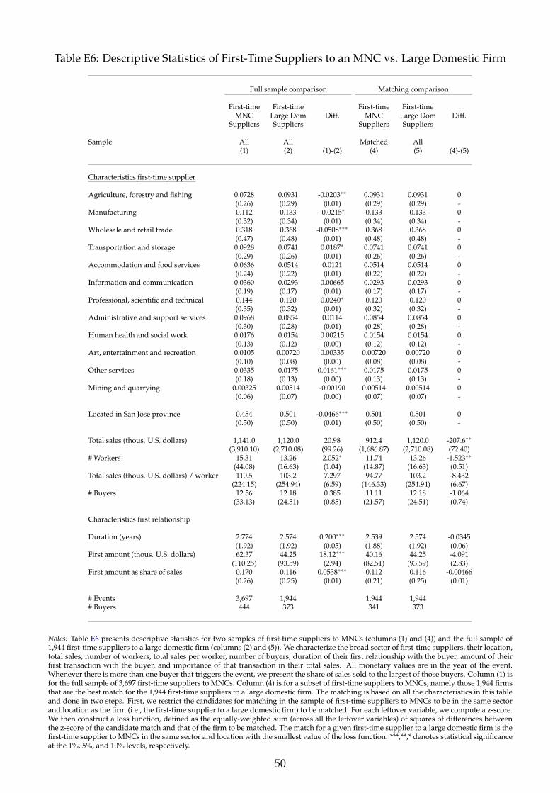
Table E6: Descriptive Statistics of First-Time Suppliers to an MNC vs. Large Domestic Firm

Full sample comparison Matching comparison

First-time First-time First-time First-timeMNC Large Dom Diff. MNC Large Dom Diff.

Suppliers Suppliers Suppliers Suppliers

Sample All All Matched All(1) (2) (1)-(2) (4) (5) (4)-(5)

Characteristics first-time supplier

Agriculture, forestry and fishing 0.0728 0.0931 -0.0203∗∗ 0.0931 0.0931 0(0.26) (0.29) (0.01) (0.29) (0.29) -

Manufacturing 0.112 0.133 -0.0215∗ 0.133 0.133 0(0.32) (0.34) (0.01) (0.34) (0.34) -

Wholesale and retail trade 0.318 0.368 -0.0508∗∗∗ 0.368 0.368 0(0.47) (0.48) (0.01) (0.48) (0.48) -

Transportation and storage 0.0928 0.0741 0.0187∗ 0.0741 0.0741 0(0.29) (0.26) (0.01) (0.26) (0.26) -

Accommodation and food services 0.0636 0.0514 0.0121 0.0514 0.0514 0(0.24) (0.22) (0.01) (0.22) (0.22) -

Information and communication 0.0360 0.0293 0.00665 0.0293 0.0293 0(0.19) (0.17) (0.01) (0.17) (0.17) -

Professional, scientific and technical 0.144 0.120 0.0240∗ 0.120 0.120 0(0.35) (0.32) (0.01) (0.32) (0.32) -

Administrative and support services 0.0968 0.0854 0.0114 0.0854 0.0854 0(0.30) (0.28) (0.01) (0.28) (0.28) -

Human health and social work 0.0176 0.0154 0.00215 0.0154 0.0154 0(0.13) (0.12) (0.00) (0.12) (0.12) -

Art, entertainment and recreation 0.0105 0.00720 0.00335 0.00720 0.00720 0(0.10) (0.08) (0.00) (0.08) (0.08) -

Other services 0.0335 0.0175 0.0161∗∗∗ 0.0175 0.0175 0(0.18) (0.13) (0.00) (0.13) (0.13) -

Mining and quarrying 0.00325 0.00514 -0.00190 0.00514 0.00514 0(0.06) (0.07) (0.00) (0.07) (0.07) -

Located in San Jose province 0.454 0.501 -0.0466∗∗∗ 0.501 0.501 0(0.50) (0.50) (0.01) (0.50) (0.50) -

Total sales (thous. U.S. dollars) 1,141.0 1,120.0 20.98 912.4 1,120.0 -207.6∗∗

(3,910.10) (2,710.08) (99.26) (1,686.87) (2,710.08) (72.40)# Workers 15.31 13.26 2.052∗ 11.74 13.26 -1.523∗∗

(44.08) (16.63) (1.04) (14.87) (16.63) (0.51)Total sales (thous. U.S. dollars) / worker 110.5 103.2 7.297 94.77 103.2 -8.432

(224.15) (254.94) (6.59) (146.33) (254.94) (6.67)# Buyers 12.56 12.18 0.385 11.11 12.18 -1.064

(33.13) (24.51) (0.85) (21.57) (24.51) (0.74)

Characteristics first relationship

Duration (years) 2.774 2.574 0.200∗∗∗ 2.539 2.574 -0.0345(1.92) (1.92) (0.05) (1.88) (1.92) (0.06)

First amount (thous. U.S. dollars) 62.37 44.25 18.12∗∗∗ 40.16 44.25 -4.091(110.25) (93.59) (2.94) (82.51) (93.59) (2.83)

First amount as share of sales 0.170 0.116 0.0538∗∗∗ 0.112 0.116 -0.00466(0.26) (0.25) (0.01) (0.21) (0.25) (0.01)

# Events 3,697 1,944 1,944 1,944# Buyers 444 373 341 373

Notes: Table E6 presents descriptive statistics for two samples of first-time suppliers to MNCs (columns (1) and (4)) and the full sample of1,944 first-time suppliers to a large domestic firm (columns (2) and (5)). We characterize the broad sector of first-time suppliers, their location,total sales, number of workers, total sales per worker, number of buyers, duration of their first relationship with the buyer, amount of theirfirst transaction with the buyer, and importance of that transaction in their total sales. All monetary values are in the year of the event.Whenever there is more than one buyer that triggers the event, we present the share of sales sold to the largest of those buyers. Column (1) isfor the full sample of 3,697 first-time suppliers to MNCs. Column (4) is for a subset of first-time suppliers to MNCs, namely those 1,944 firmsthat are the best match for the 1,944 first-time suppliers to a large domestic firm. The matching is based on all the characteristics in this tableand done in two steps. First, we restrict the candidates for matching in the sample of first-time suppliers to MNCs to be in the same sectorand location as the firm (i.e., the first-time supplier to a large domestic firm) to be matched. For each leftover variable, we compute a z-score.We then construct a loss function, defined as the equally-weighted sum (across all the leftover variables) of squares of differences betweenthe z-score of the candidate match and that of the firm to be matched. The match for a given first-time supplier to a large domestic firm is thefirst-time supplier to MNCs in the same sector and location with the smallest value of the loss function. ***,**,* denotes statistical significanceat the 1%, 5%, and 10% levels, respectively.

50

Table E7: Descriptive Statistics of First-Time Suppliers to an MNC vs. Domestic Exporter

Full sample comparison Matching comparison

First-time First-time First-time First-timeMNC Dom Expor Diff. MNC Dom Expor Diff.

Suppliers Suppliers Suppliers Suppliers

Sample All All Matched All(1) (2) (1)-(2) (4) (5) (4)-(5)

Characteristics first-time supplier

Agriculture, forestry and fishing 0.0728 0.108 -0.0355∗∗∗ 0.108 0.108 0(0.26) (0.31) (0.01) (0.31) (0.31) -

Manufacturing 0.112 0.138 -0.0259∗ 0.138 0.138 0(0.32) (0.34) (0.01) (0.34) (0.34) -

Wholesale and retail trade 0.318 0.351 -0.0330∗ 0.351 0.351 0(0.47) (0.48) (0.01) (0.48) (0.48) -

Transportation and storage 0.0928 0.0670 0.0257∗∗ 0.0670 0.0670 0(0.29) (0.25) (0.01) (0.25) (0.25) -

Accommodation and food services 0.0636 0.0391 0.0245∗∗∗ 0.0391 0.0391 0(0.24) (0.19) (0.01) (0.19) (0.19) -

Information and communication 0.0360 0.0244 0.0115∗ 0.0244 0.0244 0(0.19) (0.15) (0.01) (0.15) (0.15) -

Professional, scientific and technical 0.144 0.142 0.00144 0.142 0.142 0(0.35) (0.35) (0.01) (0.35) (0.35) -

Administrative and support service 0.0968 0.0901 0.00675 0.0901 0.0901 0(0.30) (0.29) (0.01) (0.29) (0.29) -

Human health and social work 0.0176 0.0133 0.00431 0.0133 0.0133 0(0.13) (0.11) (0.00) (0.11) (0.11) -

Art, entertainment and recreation 0.0105 0.00838 0.00217 0.00838 0.00838 0(0.10) (0.09) (0.00) (0.09) (0.09) -

Other services 0.0335 0.0154 0.0182∗∗∗ 0.0154 0.0154 0(0.18) (0.12) (0.01) (0.12) (0.12) -

Mining and quarrying 0.00325 0.00349 -0.000246 0.00349 0.00349 0(0.06) (0.06) (0.00) (0.06) (0.06) -

Located in San Jose province 0.454 0.489 -0.0344∗ 0.489 0.489 0(0.50) (0.50) (0.02) (0.50) (0.50) -

Total sales (thous. U.S. dollars) 1,141.0 1,779.0 -638.0∗∗∗ 1,343.3 1,779.0 -435.7∗∗

(3,910.10) (4,383.61) (125.99) (3,313.84) (4,383.61) (145.22)# Workers 15.31 25.72 -10.40∗∗∗ 21.34 25.72 -4.376

(44.08) (71.70) (1.66) (58.64) (71.70) (2.45)Total sales (thous. U.S. dollars) / worker 110.5 100.3 10.15 95.52 100.3 -4.824

(224.15) (125.90) (6.28) (121.23) (125.90) (4.62)# Buyers 12.56 19.66 -7.094∗∗∗ 16.95 19.66 -2.703

(33.13) (40.88) (1.10) (32.82) (40.88) (1.39)

Characteristics first relationship

Duration (years) 2.774 2.325 0.449∗∗∗ 2.293 2.325 -0.0321(1.92) (1.76) (0.06) (1.72) (1.76) (0.07)

First amount (thous. U.S. dollars) 62.37 39.50 22.87∗∗∗ 38.53 39.50 -0.968(110.25) (95.05) (3.31) (92.06) (95.05) (3.50)

First amount as share of sales 0.170 0.0894 0.0809∗∗∗ 0.0918 0.0894 0.00240(0.26) (0.20) (0.01) (0.20) (0.20) (0.01)

# Events 3,697 1,432 1,432 1,432# Buyers 444 385 323 385

Notes: Table E7 presents descriptive statistics for two samples of first-time suppliers to MNCs (columns (1) and (4)) and the full sample of1,432 first-time suppliers to a domestic exporter (columns (2) and (5)). We characterize the broad sector of first-time suppliers, their location,total sales, number of workers, total sales per worker, number of buyers, duration of their first relationship with the buyer, amount of theirfirst transaction with the buyer, and importance of that transaction in their total sales. All monetary values are in the year of the event.Whenever there is more than one buyer that triggers the event, we present the share of sales sold to the largest of those buyers. Column (1) isfor the full sample of 3,697 first-time suppliers to MNCs. Column (4) is for a subset of first-time suppliers to MNCs, namely those 1,432 firmsthat are the best match for the 1,432 first-time suppliers to a domestic exporter. The matching is based on all the characteristics in this tableand done in two steps. First, we restrict the candidates for matching in the sample of first-time suppliers to MNCs to be in the same sectorand location as the firm (i.e., the first-time supplier to a domestic exporter) to be matched. For each leftover variable, we compute a z-score.We then construct a loss function, defined as the equally-weighted sum (across all the leftover variables) of squares of differences betweenthe z-score of the candidate match and that of the firm to be matched. The match for a given first-time supplier to a domestic exporter is thefirst-time supplier to MNCs in the same sector and location with the smallest value of the loss function. ***,**,* denotes statistical significanceat the 1%, 5%, and 10% levels, respectively.

51

−.2

0.2

.4O

utc

om

e:

To

tal S

ale

s

−4 −3 −2 −1 0 1 2 3 4

Year Since Event

MNCs (matched) Government

(a) Total Sales, Government

−.2

0.2

.4O

utc

om

e:

Nu

mb

er

of

Wo

rke

rs

−4 −3 −2 −1 0 1 2 3 4

Year Since Event

MNCs (matched) Government

(b) Number of Workers, Government

−.2

0.2

.4O

utc

om

e:

To

tal S

ale

s

−4 −3 −2 −1 0 1 2 3 4

Year Since Event

MNCs (matched) Large Domestic Buyers

(c) Total Sales, Large Domestic Firm

−.2

0.2

.4O

utc

om

e:

Nu

mb

er

of

Wo

rke

rs

−4 −3 −2 −1 0 1 2 3 4

Year Since Event

MNCs (matched) Large Domestic Buyers

(d) Number of Workers, Large Domestic Firm

−.2

0.2

.4O

utc

om

e:

To

tal S

ale

s

−4 −3 −2 −1 0 1 2 3 4

Year Since Event

MNCs (matched) Domestic Exporters

(e) Total Sales, Domestic Exporter

−.2

0.2

.4O

utc

om

e:

Nu

mb

er

of

Wo

rke

rs

−4 −3 −2 −1 0 1 2 3 4

Year Since Event

MNCs (matched) Domestic Exporters

(f) Number of Workers, Domestic Exporter

Figure E1: The Effects of Three Placebo Events on Total Sales and Employment: First-TimeSupplying to the Government, a Large Domestic Buyer, or a Domestic Exporter

Notes: Figure E1 compares the effects of the event of starting to supply to an MNC with those from three otherplacebo events, namely starting to supply to (i) the Costa Rican government (panels E1a and E1b); (ii) a largedomestic firm (panels E1c and E1d); and (iii) a domestic exporter (panels E1e and E1f). We show these effectsfor two outcomes variables: log total sales (left-hand side panels) and log number of workers (right-hand sidepanels). The vertical lines reflect the 95% confidence intervals. For comparability, in each figure, we contrast theeffects on the sample of first-time suppliers to the government, large domestic buyer, or domestic exporter tothose for a matched subset from the baseline sample of first-time suppliers to MNCs. For example, to constructthis subset for the government, we start from the sample of first-time suppliers to the government. Then, for eachfirm in that sample, we identify the best match in the baseline sample of first-time suppliers to MNCs (where thematching is based on their similarity in supplier characteristics and the demand shock experienced during theircorresponding event). For more details on this matching procedure, see Section 5.1 and Tables E5 to E7.

52

−.2

0.2

.4O

utc

om

e:

Nu

mb

er

of

Oth

er

Co

rp.

Bu

ye

rs

−4 −3 −2 −1 0 1 2 3 4

Year Since Event

MNCs (matched) Government

(a) Number Other Buyers, Government

−1

−.5

0.5

Ou

tco

me

: A

ve

rag

e C

orp

. S

ale

s t

o O

the

rs

−4 −3 −2 −1 0 1 2 3 4

Year Since Event

MNCs (matched) Government

(b) Average Sales Others, Government

−.2

0.2

.4O

utc

om

e:

Nu

mb

er

of

Oth

er

Co

rp.

Bu

ye

rs

−4 −3 −2 −1 0 1 2 3 4

Year Since Event

MNCs (matched) Large Domestic Buyers

(c) Number Other Buyers, Large Domestic Firm

−1

−.5

0.5

Ou

tco

me

: A

ve

rag

e C

orp

. S

ale

s t

o O

the

rs

−4 −3 −2 −1 0 1 2 3 4

Year Since Event

MNCs (matched) Large Domestic Buyers

(d) Average Sales Others, Large Domestic Firm

−.2

0.2

.4O

utc

om

e:

Nu

mb

er

of

Oth

er

Co

rp.

Bu

ye

rs

−4 −3 −2 −1 0 1 2 3 4

Year Since Event

MNCs (matched) Domestic Exporters

(e) Number Other Buyers, Domestic Exporter

−1

−.5

0.5

Ou

tco

me

: A

ve

rag

e C

orp

. S

ale

s t

o O

the

rs

−4 −3 −2 −1 0 1 2 3 4

Year Since Event

MNCs (matched) Domestic Exporters

(f) Average Sales Others, Domestic Exporter

Figure E2: The Effects of Three Placebo Events on the Number of Other Corporate Buyers andAverage Sales to Other Corporate Buyers: First-Time Supplying to the Government, LargeDomestic Buyer, or Domestic Exporter

Notes: Figure E2 compares the effects of the event of starting to supply to an MNC with those from three otherplacebo events, namely starting to supply to (i) the Costa Rican government (panels E2a and E2b); (ii) a largedomestic firm (panels E2c and E2d); and (iii) a domestic exporter (panels E2e and E2f). We show these effects fortwo outcomes variables: log number of other corporate buyers (left-hand side panels) and log average sales toother corporate buyers (right-hand side panels). The vertical lines reflect the 95% confidence intervals. For com-parability, in each figure, we contrast the effects on the sample of first-time suppliers to the government, largedomestic buyer, or domestic exporter to those for a matched subset from the baseline sample of first-time sup-pliers to MNCs. For example, to construct this subset for the government, we start from the sample of first-timesuppliers to the government. Then, for each firm in that sample, we identify the best match in the baseline sampleof first-time suppliers to MNCs (where the matching is based on their similarity in supplier characteristics andthe demand shock experienced during their corresponding event). For more details on this matching procedure,see Section 5.1 and Tables E5 to E7.

53

Online Appendix E.3 Model-Based Estimation of the Short and Medium-

Run Marginal Cost Elasticity

Online Appendix E.3.1 Total Cost Function Encompasses the Cobb–Douglas and CESCases

In equation (3) of the paper we assume that the supplier produces a total quantity Qi

with a total cost function given by

TC(Qi) = κi

(Qi

φi

)γ+1

(E1)

where γ > −1, φi refers to physical efficiency, and κi is a constant. We show hereafter thatwhen all inputs are flexible, the total cost function in equation (3) encompasses both Cobb–Douglas and general returns to scale CES production functions. Moreover, we also show thatwhenever all inputs are flexible, 1/(γ+ 1) can be interpreted as the returns to scale of the firm.In the remainder of this section, we abstract from the subindex i for simplicity.

Cost function in the Cobb–Douglas case. Define the production function as Q = φLαL KαK

and assume no fixed costs. Let W be the price of L and let R be the price of K. We can thenwrite the total cost function TC(Q) as:

TC(Q) =αL + αk(

ααLL + ααK

K) 1

αL+αK

WαL

αL+αK RαK

αL+αK

(Qφ

) 1αL+αK

= κ(W, R)(

Qφ

) 1αL+αK

= κ(W, R)(

Qφ

) 1ξ

,

where ξ = αL + αK is the returns to scale of the production function, and κ(., .) is a function ofthe input prices. If we assume that firms are input-price takes, then we can take κ(W, R) as aconstant κ. Mapping back to equation (3) we notice that ξ = 1/(γ + 1).

Cost function in the CES case. The general returns CES production function is given by

Q = φ [αLLρ + αKKρ]ξρ , where ξ is the returns to scale of the production function. Assume

again no fixed cost. We can then write the total cost function TC(Q) as:

TC(Q) =

[α

11+ρ

L Wρ

ρ+1 + α1

1+ρ

K Kρ

ρ+1

] 1+ρρ(

Qφ

) 1ξ

= κ′(W, R)(

Qφ

) 1ξ

,

where κ′(W, R) is again a function of input prices. With the same assumption of input-price-taker behaviour, we can take κ′(W, R) to be a constant κ. Mapping back to equation (3) wenotice that ξ = 1/(γ + 1).

Online Appendix E.3.2 Model Derivations

Consider a set of domestic supplier firms indexed by i selling a variety of a good tobuyers indexed by j. We assume that supplier i faces an isoelastic demand from buyer j givenby qij = bij p−σ

i , where qij denotes the units of output that buyer j demands from supplier i,

54

bij ≡(

b∗ij)σ−1

is a demand shifter that depends on the market and buyer j’s characteristics,pi is the price that supplier i charges, and σ > 1 is the elasticity of demand. The supplierproduces a total quantity Qi = ∑j qij with a total cost function given by:

TC(Qi) = κi

(Qi

φ∗i

)γ+1

where γ > −1, φ∗i refers to physical efficiency, and κi is a constant. The firm charges pi =

µi MC(Qi), where µi = σσ−1 is a constant markup and MC(Qi) = ∂TC(Qi)

∂Qiis the marginal

cost. This means that the price is given by pi = µi MC(Qi) = µi (γ + 1) κiQγi(φ∗i)−(γ+1)

=

ci,0Qγi(φ∗i)−(γ+1) , where ci,0 ≡ µi (γ + 1) κi. We can also write total production as:

Qi = ∑j

(b∗ij)σ−1

p−σi =

[ci,0Qγ

i (φ∗i )−(γ+1)

]−σ

∑j

(b∗ij)σ−1

= Q−γσi c−σ

i,0 (φ∗i )σ(γ+1) (B∗i )

σ−1 ,

where B∗i =

(∑j

(b∗ij)σ−1

) 1σ−1

. The previous equation implies:

Qi = c−σ

1+γσ

i,0 (φ∗i )σ(γ+1)1+γσ (B∗i )

σ−11+γσ . (E2)

Denote total revenues as Ri = piQi. We can write Ri as:

Ri = ci,0Qγ+1i (φ∗i )

−(γ+1) = c−(σ−1)

1+γσ

i,0 (φ∗i )(σ−1)(γ+1)

1+γσ (B∗i )(σ−1)(γ+1)

1+γσ .

For future reference note that:

B∗i = ci,1R1+γσ

(σ−1)(γ+1)i (φ∗i )

−1 , (E3)

where ci,1 ≡ c1

γ+1i,0 .

Consider now an event where the supplier i starts selling an amount Ri,M ≡ piqi,M to agiven firm M. Define sales to firms other than M (“sales to others” henceforth) as Ri ≡ piQi,where Qi = ∑j 6=M qij. Note that under this definition, we have the identity Ri ≡ Ri + Ri,M.Our objective is to write Ri as a function of Ri, which are two observable variables in our data.To this end, first note that:

Qi = ∑j 6=M

qij = ∑j 6=M

(b∗ij)σ−1

p−σi = p−σ

i ∑j 6=M

(b∗ij)σ−1

= Q−γσi c−σ

i,0 (φ∗i )σ(γ+1) (B∗i )σ−1 ,

where B∗i =(

∑j 6=M bσ−1ij

) 1σ−1 . The previous equation implies:

Ri =piQi =[ci,0Qγ

i (φ∗i )−(γ+1)

] [Q−γσ

i c−σi,0 (φ∗i )

σ(γ+1) (B∗i )σ−1]

55

=Qγ(1−σ)i c(1−σ)

i,0 (φ∗i )(σ−1)(γ+1) (B∗i )σ−1 .

Replacing Qi from equation (E2), we have:

Ri =

[c−σ

1+γσ

i,0 (φ∗i )σ(γ+1)1+γσ (B∗i )

σ−11+γσ

]γ(1−σ)

c(1−σ)i,0 (φ∗i )

(σ−1)(γ+1) (B∗i )σ−1

= ci,2(

B∗i)σ−1

(φ∗i )(σ−1)(γ+1)

1+γσ (B∗i )− (σ−1)2γ

1+γσ ,

where ci,2 ≡ c1−σ

1+γσ

i,0 . Replacing B∗i from equation (E3) we get:

Ri = ci,2(

B∗i)σ−1

(φ∗i )(σ−1)(γ+1)

1+γσ

[ci,1R

1+γσ(σ−1)(γ+1)i (φ∗i )

−1

]− (σ−1)2γ1+γσ

= ci,3R− (σ−1)γ

γ+1i (φi)

σ−1 ,

where ci,3 ≡ ci,2c− (σ−1)2γ

1+γσ

i,1 = c1−σγ+1i,0 and φi = B∗i φ∗i . Taking log differences of the optimal sales to

others the year before versus τ years after the event, we find:

∆τ ln(Ri) = δ∆τ ln(Ri + Ri,M) + (σ− 1)∆τ ln(φi), (E4)

where δ ≡ − (σ−1)γγ+1 and Ri ≡ Ri + Ri,M. This is equation (4) in the main text (see Section 5.2).

Online Appendix E.3.3 A Brief Discussion on an Extension with Variable Markups

As in the section before, assume that a supplier i sells to buyers indexed by j a quantityqij such that the total production of supplier i is Qi ≡ ∑j qij. Supplier i faces a demand qij =

Dj(bij, pi) from each buyer j, where Dj(., .) is the demand function, bij is demand shifter (thatcould be interpreted as an adjustment of the price for the quality or appeal of the good ofsupplier i, among others) and pi is the price charged by supplier i. We assume

∂logDj∂logbij

> 0.Profit maximization implies pi =

ε1+ε MC(Qi) = µ(Qi)mc(Qi), where ε ≤ 0 is the elas-

ticity of the aggregate demand that supplier i faces with respect to price pi, MC(Qi) is themarginal cost of production, and µ(Qi) is a potentially-variable markup.

Denote the sales to buyer j as Rij = piqij. Then define x = dlog(x) as the percentagechange in variable x. The partial equilibrium comparative statics imply that

Rij = pij + qij = µ(Qi) + MC(Qi) +∂logDj

∂logpi(µ(

Qi) + MC(Qi))+

∂logDj

∂logbijbij

=(1 + ε j

)µ(Qi) +

((1 + ε j

)MC(Qi) +

∂logDj

∂logbijbij

), (E5)

where ε j ≡∂logDj∂logpi

is the demand elasticity. ε j < −1 is empirically supported both in ourcontext (see Online Appendix E.3.4) and in the broader literature (see Head and Mayer, 2014).The argument that follows assumes that ε j < −1, hence that

(1 + ε j

)< 0.

56

We are interested under which conditions an increase in sales to other buyers j is at oddswith an increase in markups alone. Equation (E5) shows that without a fall in marginal costsand/or an increase in the demand shifter that are large enough to compensate for the rise inmarkups, a rise in markups alone would lead to a fall in sales to buyer j. As our data does nottrack prices, quantities, and product characteristics separately, we consider improvements inphysical efficiency and quality to be isomorphic.

Online Appendix E.3.4 Inferring σ from DLW (2012)

Table E8: Inferred σ and Returns to Scale Parameter from the Method of DLW (2012)

Labor Capital µ Returns σ Numberto scale of obs

(1) (2) (3) (4) (5) (6)

All sectors (pooled) 0.84 0.08 1.25 0.92 5.03 82,094(0.00) (0.00) (0.00) (0.00) (0.08)

Agriculture, forestry and fishing 0.68 0.09 1.12 0.77 9.20 5,229(0.01) (0.01) (0.02) (0.01) (1.38)

Manufacturing 0.88 0.08 1.19 0.96 6.21 14,922(0.02) (0.00) (0.03) (0.02) (0.83)

Wholesale and retail trade 0.81 0.08 1.25 0.88 4.98 42,033(0.00) (0.01) (0.01) (0.01) (0.11)

Transportation and storage 1.00 0.04 1.57 1.03 2.74 1,375(0.11) (0.06) (0.18) (0.12) (1.98)

Accommodation and food services 0.77 0.07 1.05 0.84 20.88 9,280(0.04) (0.01) (0.05) (0.03) (8.46)

Information and communication 0.82 0.08 1.21 0.90 5.87 896(0.16) (0.06) (0.25) (0.14) (24.62)

Professional, scientific and technical 0.88 0.09 1.29 0.98 4.44 3,432(0.01) (0.01) (0.02) (0.02) (0.30)

Administrative and support services 0.88 0.05 1.21 0.93 5.80 1,998(0.03) (0.02) (0.04) (0.03) (1.51)

Human health and social work 0.86 0.09 1.36 0.95 3.81 861(0.18) (0.06) (0.29) (0.16) (7.61)

Other services 0.85 0.02 1.26 0.83 4.92 1,275(0.18) (0.08) (0.31) (0.17) (13.84)

Notes: Table E8 shows results from the De Loecker and Warzynski (2012) methodology for the economy-widesample, first pooled across all sectors (see upper panel) and then separately by sector (see lower panel). Column(1) and (2) show the estimated input elasticities for labor and capital (measured as net assets) in a Cobb–Douglasvalue-added production function. Column (3) shows the markup (µ). Column (4) corresponds to the returns toscale parameter, which is calculated as the sum of columns (1) and (2). Column (5) corresponds to the inferredelasticity of demand (σ). Our assumption of CES demand for buyers implies a constant markup over marginalcost given by µ = σ

σ−1 , which allows us to infer σ from our estimated µ. Finally, column (6) reports the numberof observations. Bootstrap standard errors are shown in parenthesis.

We infer the elasticity of demand σ from the markup estimation method of De Loeckerand Warzynski (2012) combined with our model. By assuming a Cobb–Douglas productionfunction specification, we first estimate the firm-level markup (µ). Under the assumption of

57

constant elasticity of demand (σ), we then infer σ from the markup (since the markup is givenby µ = σ

σ−1 ). Using this approach, we estimate an average markup across sectors of 1.248 (25%over marginal cost). This implies σ = 5.03. A value of σ = 5 value is central in the range ofestimates used in the international trade literature (see Head and Mayer, 2014).

Online Appendix E.3.5 Additional Estimates of δ and γ

Table E9: Model-Based Estimates of the Marginal Cost Elasticity

First-time First-time First-time First-timeMNC suppliers Government suppliers Dom. exp. suppliers Large dom. suppliers

δ γ δ γ δ γ δ γ

(1) (2) (3) (4) (5) (6) (7) (8)

Year of event -2.702∗∗∗ 2.034 -2.988∗∗∗ 2.867 -1.691∗∗∗ 0.723∗∗ -3.679∗∗∗ 10.473(0.550) (1.255) (0.919) (3.411) (0.419) (0.308) (0.588) (19.210)

1 year after event -0.654∗∗∗ 0.194∗∗∗ -1.419∗∗∗ 0.544∗ -0.635∗∗ 0.187∗ -0.906∗∗∗ 0.290∗∗

(0.158) (0.056) (0.534) (0.316) (0.296) (0.103) (0.322) (0.133)2 years after event -0.435∗∗∗ 0.121∗∗∗ -1.145∗ 0.397 -0.493∗ 0.140 -0.237 0.062

(0.120) (0.038) (0.602) (0.292) (0.268) (0.086) (0.402) (0.113)3 years after event -0.464∗∗∗ 0.130∗∗∗ -1.768 0.781 -0.900∗∗ 0.287∗ -0.753∗∗ 0.230∗

(0.156) (0.049) (1.493) (1.176) (0.387) (0.159) (0.365) (0.137)4 years after event -0.433∗∗ 0.120∗∗ -1.295 0.473 -1.179∗ 0.414 -0.966 0.315

(0.169) (0.053) (1.474) (0.794) (0.651) (0.323) (0.642) (0.276)

# Observations 116,683 116,683 149,686 149,686 142,161 142,161 130,422 130,422

Notes: Table E9 shows the estimates of δ (the parameter that governs the interdependence between the change intotal sales of firm i and its change in sales to others) and the marginal cost elasticity γ = −δ/(δ + σ− 1). Theirestimation is based on equation (5). For these estimates, we set σ = 5.03, which we infer from the average markupin the economy using the methodology of De Loecker and Warzynski (2012). All columns use the total sales andsales to others constructed from the corporate income tax returns. Columns (1) and (2) show our baseline results,where we leverage our event-study specification for the case of first-time suppliers to MNCs (i.e., firm M is thefirst MNC buyer). These are the same results as those shown in columns (1) and (2) of Table 5. Columns (3) and(4) switch to the event being defined as the first time supplying to the government. Columns (5) and (6) switch tothe event being defined as the first time supplying to a domestic exporter. Columns (7) and (8) switch to the eventbeing defined as the first time supplying to a large domestic firm. These events in columns (3) to (8) correspondto the ones described in Section 5.1. In these cases, we further assume that the firm-level productivity does notchange after these events. This assumption is in line with our evidence in Figure 3 (left-hand side panels). Weobtain standard errors for our estimates of δ using a bootstrap procedure. Since γ is a function of δ, we then applythe delta method to obtain standard errors for our estimates of γ. ***,**,* denotes statistical significance at the 1%,5%, and 10% levels, respectively.

58

Online Appendix E.4 Ruling Out Changes in Tax Evasion Behavior

Table E10: Similar Compliance in Third Party Reporting After Supplying to an MNC

Seller-Diff Buyer-Diff Mis-Seller Seller-Diff Buyer-Diff Mis-Seller(1) (2) (3) (4) (5) (6)

4 years before event 0.002 0.003 0.002 0.012 0.008 -0.002(0.006) (0.008) (0.003) (0.017) (0.013) (0.005)

3 years before event 0.002 0.001 0.001 0.010 0.007 -0.004(0.007) (0.007) (0.002) (0.013) (0.010) (0.004)

2 years before event -0.002 -0.004 -0.002 0.005 -0.003 -0.000(0.004) (0.005) (0.003) (0.009) (0.007) (0.003)

Year of event 0.000 0.001 0.000 -0.003 -0.003 0.002(0.005) (0.005) (0.002) (0.007) (0.006) (0.002)

1 year after event 0.007∗ 0.006 -0.001 -0.002 -0.004 0.005(0.004) (0.007) (0.002) (0.011) (0.010) (0.004)

2 years after event 0.008∗ 0.005 -0.001 -0.006 -0.010 0.006(0.005) (0.006) (0.002) (0.015) (0.015) (0.006)

3 years after event 0.004 0.000 -0.002 -0.015 -0.018 0.006(0.005) (0.006) (0.002) (0.020) (0.018) (0.007)

4 years after event 0.014∗∗ 0.009 -0.003 -0.012 -0.014 0.008(0.006) (0.006) (0.003) (0.024) (0.023) (0.009)

Mean Dep. Var. (level) 0.038 0.048 0.012 0.074 0.061 0.013SD Dep. Var. (level) 0.15 0.15 0.073 0.20 0.17 0.058

Firm FE Yes Yes Yes Yes Yes YesYear-4DSect-Prov FE Yes Yes Yes Yes Yes YesNever Suppliers Yes Yes Yes No No No

Adjusted R2 0.19 0.12 0.15 0.15 0.10 0.045# Observations 109,438 109,438 109,438 23,677 23,677 23,677# Fixed Effects 24,115 24,115 24,115 7,323 7,323 7,323# Firms 17,129 17,129 17,129 3,472 3,472 3,472

Notes: Table E10 shows the results of running specification (1) adapted to three measures of quality in third-partyreporting. For this exercise, we use the raw version of D-151, as opposed to the clean version used in the baselineanalysis (see Online Appendix A.1.2). “Seller-diff” is a weighted average of the percentage difference in valuesreported, across all transactions in a year for which a firm is the seller. The percentage difference is computedas the (maximum value reported-minimum value reported)/(minimum value reported). “Seller-diff” uses asweights the importance of the transaction in that year for the seller. “Buyer-diff” is analogously constructed, thistime keeping only transactions for which a firm is the buyer. “Mis-Seller” is defined as (the total number of buyersthat reported a given firm as a seller and that are not reported back by the seller)/(the total number of buyers ofthe seller that are reported by either side). The event is defined as a first time sale to an MNC. Columns (1) to(3) report event study estimates for the sample including both domestic firms that become first-time suppliers toan MNC after 2010 and domestic firms never observed as supplying to an MNC during our entire firm-to-firmtransaction data. Clustering of standard errors is at the two-digit sector by province level. Columns (4) to (6)focus only on the sample of domestic firms becoming first-time suppliers to an MNC between 2010 and 2015 anduse standard error clustering at event by province level. Robust standard errors in parentheses. ***,**,* denotesstatistical significance at the 1%, 5%, and 10% levels, respectively.

59

Table E11: No Changes After the Event in the Share of New Hires in Year t Who Were EitherNonemployed or Informal Workers (or Newly-Arrived Foreign Workers) in Year (t− 1)

Excludes foreign workers No Yes No Yes(1) (2) (3) (4)

4 years before event 0.007 0.002 0.010 -0.000(0.018) (0.018) (0.025) (0.022)

3 years before event -0.007 -0.014 -0.012 -0.022(0.012) (0.010) (0.018) (0.017)

2 years before event -0.019∗∗ -0.014 -0.017 -0.017(0.008) (0.009) (0.010) (0.011)

Year of event -0.001 0.000 0.004 0.006(0.008) (0.009) (0.010) (0.009)

1 year after event 0.001 -0.003 0.004 0.004(0.008) (0.007) (0.014) (0.017)

2 years after event 0.005 0.000 0.014 0.013(0.009) (0.007) (0.016) (0.019)

3 years after event -0.001 -0.003 0.006 0.009(0.010) (0.010) (0.022) (0.025)

4 years after event 0.019∗ 0.014 0.027 0.028(0.010) (0.009) (0.024) (0.028)

Mean Dep. Var. (level) 0.0026 0.0025 0.0026 0.0025SD Dep. Var. (level) 0.0011 0.0010 0.0010 0.0010

Never Suppliers Yes Yes No NoAdjusted R2 0.093 0.079 0.087 0.071# Observations 116,683 116,683 23,961 23,961# Fixed Effects 25,174 25,174 7,366 7,366# Firms 18035 18035 3482 3482

Notes: Table E11 shows the effects of starting to supply to an MNC on the share of new workers hired by firmi in year t who could not be found in year (t− 1) in the matched employer-employee data (MEED) from CR’sSocial Security Fund (because they were either nonemployed, informal workers, or coming from abroad in year(t− 1)). Columns (1) and (2) use the full sample (with both domestic firms that become first-time suppliers toan MNC between 2010 and 2015 and domestic firms never observed as supplying to an MNC), while columns(3) and (4) use the restricted sample (with only the firms that eventually become first-time suppliers to MNCs).The difference between column (1) vs. (2) and columns (3) vs. (4) is that columns (2) and (4) exclude foreignworkers. Columns (1) and (3) present a conservative analysis as they already include foreign workers as potential“outsiders” to the MEED. To avoid capturing workers coming directly from the university, we restrict the MEEDsample to workers born in 1978 or before (to be at least age 30 in 2008). We also drop workers older than 60 atany point. When we aggregate the data at an annual level, we define a worker’s employer in t as the firm wherethe worker made most of her yearly earnings in t. A “new hire” of firm i in year t is a worker who works at firm iin t but did not work at firm i in (t− 1). Given the restrictions described above, if a worker is not observed in theMEED in year (t− 1), then the worker was either nonemployed that year or had an informal employer who didnot make social security contributions on her behalf (or is a foreign worker who has just entered the Costa Ricanlabor market, in the case of columns (1) and (3)). A firm that formalizes in year t its already incumbent workersshould display a larger share of “new hires” whose employment status in year (t− 1) was either nonemploymentor informality. Note that this is not a sufficient condition. Firms might be legitimately expanding their workforceby hiring workers who were either nonemployed or informal prior (but without any attachment to their newemployer). We use the same firm and four-digit sector × province × calendar year fixed effects as in the baselineexercises and the same clustering (two-digit sector × province in the full sample and province × event year inthe restricted one). ***,**,* denotes statistical significance at the 1%, 5%, and 10% levels, respectively.

60

Online Appendix F Surveys

Online Appendix F.1 Survey Design and Implementation

We targeted with surveys the domestic firms in three groups. First, we targeted a 20%random sample of the 3,813 domestic firms experiencing an event in the economy-wide sam-ple (3,813 firms that experienced a first-time supplying event with an MNC between 2010 to2015),xx that is, 762 domestic firms. Second, we targeted all the winning firms in the “Produc-tive Linkages” Procomer sample (31 firms). Finally, we targeted all other domestic firms thatstarted supplying to MNCs through Procomer (385-31=354 firms). It was essential to includethe first sample, as it is the one generating our baseline results. The second sample is the basisof one of our main robustness checks. Most of the firms in the last sample are experiencedsuppliers and can bring a long-term perspective on their relationships to MNCs. In additionto the domestic firms in these three groups, we also targeted all the MNCs that served as firstMNC buyers to these domestic firms (471, 53, and 163 respectively).xxi

Surveys had two core objectives: inquire on specific threats to identification and shedlight on features of linkages between MNCs and their new suppliers that are unobservable inadministrative data. We designed four surveys: two for domestic firms and two for MNCs.For each type of firm (domestic or MNC), we wrote a short and a long version of the survey.The short version of the survey focuses only on the core topics. The long version requests moredetails on the core topics, in addition to more information useful for context.

The co-authors of this project designed the survey instruments. BCCR, Procomer, andCINDE provided feedback that improved the initial drafts.xxii We first wrote the question-naires in English. Once we refined the order, structure, and wording of questions, a nativeSpanish speaker translated the questionnaires. We only conducted one round of surveys, allof which took place between June and September of 2018.

Long version. Long surveys were conducted in person and lasted 45 minutes to an hour.Procomer or CINDE established the first contact with firms by email. The email contained anofficial letter from BCCR describing the study and guaranteeing a fully-secured treatment ofthe data collected. Once a firm agreed to participate, our team would be granted permission

xxThere are 3,813 domestic firms that became first-time suppliers to 471 MNCs. However, in the main event-studyregression (1) studying the impact on total sales, only 3,697 of these domestic firms are used in the estimation,with the rest being dropped due to the fine set of fixed effects used.

xxiThese three sets of MNCs are overlapping as the same MNC can trigger events of the three types: economy-wide (unmediated), mediated by Procomer after 2009 and in our sample of analysis, or mediated by Procomerin any year and not part of our sample of analysis. Note also that some MNCs trigger events for more than onesupplier; that explains why the number of MNCs triggering events can be smaller than the number of domesticfirms experiencing the events. That said, it can also be that some suppliers sell to more than one MNC in thefirst year in which they sell to at least one MNC (the year of the event); that explains why the number of MNCstriggering events can also be larger than the number of domestic firms experiencing the events.

xxiiAll three entities frequently survey firms in CR.

61

to contact the firm directly in order to set up the survey meeting.xxiii

We decided to apply the long version of the survey to the firms involved in the “Produc-tive Linkages” design, that is to the 31 domestic suppliers experiencing the eligible Procomerevents and the MNC buyers that triggered those events. This choice has two advantages. First,these are firms for which we had more reliable contacts (from either Procomer or CINDE); thisimproved the chance of a positive response to our request. Second, all of these firms had otherdeals (with domestic suppliers/MNCs) that were not mediated by Procomer. Applying thelong version of the survey to these firms allowed us to inquire whether deals mediated byProcomer were different or not from unmediated deals.

The first in-person surveys served as the pilot, allowing the team to test not only thequestionnaire, but also the survey protocols and logistics. For this reason, at least one of theco-authors joined these first meetings. Once this piloting phase ended, a team of two enu-merators split the remaining in-person surveys among themselves. In the summer of 2018,both enumerators were in their final year of undergraduate studies in economics at the mainnational university. Enumerators went unaccompanied to their meetings, to avoid any risk ofanswers being influenced by either a Government official or our team.

The team agreed with BCCR, CINDE, and Procomer to share only the aggregated find-ings of the surveys. Enumerators made sure that firms knew that their specific answers werenot to be shared with these public entities. This measure was meant to create an environ-ment of trust and elicit truthful responses. Also, as almost all questions did not refer to the“Productive Linkages” program but focused on MNC-supplier relationships more broadly,enumerators clarified that surveys were not meant for program evaluation.

Figure F1 is a collage of four photographs taken by the authors during survey visits tofour domestic suppliers to MNCs. All four firms have responded to the in-person long survey.The collage showcases the diversity of the surveyed domestic firms.

Short version. Short surveys were designed to be filled in online through a Google Formand take 15 to 20 minutes. The person filling in the survey would do so in the absence of anyGovernment official or team member. In the invitation email, we included an official phonenumber and email address, in case the firm had any inquiries. We received few inquiries - ofthose, most were concerned whether the survey was legitimate or an imposture.

The invitation to participate in the online survey was sent to the firms that we targetedfrom the economy-wide sample of events (762 domestic firms and 471 MNCs) and to the firmsinvolved in Procomer events that are not part of our sample of analysis (354 domestic firmsand 163 MNCs).xxiv

Depending on the firm, the invitation was sent by Procomer, CINDE, or BCCR. Procomerand CINDE had readily-available email addresses of specific key employees in each firm. As

xxiiiProcomer contacted domestic suppliers and MNCs as part of their “Productive Linkages” database. CINDEcontacted MNCs under the Free Trade Zone regime. Unless a firm agreed to participate in the survey, the emailaddress of their contact was not revealed to our team.

xxivAgain, note that while the sets of domestic firms in these different samples are disjoint, the sets of MNCs trigger-ing the events are not.

62

Procomer and CINDE contacted firms in their portfolio, this also reassured firms on the inten-tion of the survey. Both factors significantly increased the likelihood of an answer.

BCCR contacted firms in the economy-wide restricted sample. Our team had to search forappropriate contacts from scratch. This step was the most challenging in the implementationof the surveys. Whenever firms could be found online with more than a phone number anda physical address, the most direct contact available was either a general email address (e.g.,info@firm.cr) or a contact form on the website. To increase the likelihood of an answer, thetwo enumerators made calls to all firms with a phone number, describing the survey andrequesting a direct email address of the person most qualified to answer the survey. Despitecalls being made from an official BCCR number, many firms distrusted the calls and refusedto share a personal email address.

We made up to six attempts to contact each firm. Depending on the available/preferredmode of contact, these attempts were either callbacks or email reminders. An unexpectedchallenge for the short survey came from the fact that certain corporate anti-virus softwaredirected our email to the spam folder of the recipient, as it contained the link to the survey.Recipients were also advised against clicking on the link, to avoid phishing or malware down-loads. Receiving the email from an official email address was not sufficient reassurance forsome firms. One goal behind our persistent attempts was to bring reassurance on the safety ofparticipating in the survey.

It is important to emphasize that surveys to both MNCs and domestic suppliers requiredspecific knowledge about relationships between MNCs and domestic suppliers. Our idealrespondent was the employee whose job attributes and tenure with the firm allowed him/herto provide the most accurate answers. Questions to MNCs did not require the respondent towitness the first linkage to a specific domestic supplier. However the respondent had to bewell-informed on the local procurement practices of the MNC. For this reason, we aimed tosurvey the supply chain (procurement, operations) manager of each MNC.

For domestic suppliers, part of the questions was retrospective. This required from therespondent to have worked at the firm before and during the first deals with MNCs. Giventhis constraint and the fact that most firms are small family-owned businesses, the ideal re-spondent was the founder of the firm (who is typically the general manager as well). Theretrospective nature of the survey to domestic suppliers is unlikely to have jeopardized an-swer quality for two reasons. First, most questions did not ask for specific details on the firstdeal with an MNC, details which might otherwise be affected by the time lag. Second, surveyanswers show that the first deals with MNCs were transformative for the domestic firm. Thus,it is unlikely for the firm founder to misremember the circumstances of those deals.

We went to great lengths to identify the most suitable respondent inside each firm andmake sure this person actually answered the survey. The supply chain manager of the MNCand the owner of the domestic firm are typically busy and inaccessible. Most firms do not evenpublicize the names of people in these positions, as to avoid their being pursued with unso-licited business proposals. It took considerable effort to ensure that our survey was known to

63

and answered by the right person within each firm.

Figure F1: Four Examples of Domestic Suppliers to MNCs

Notes: Figure F1 is a collage of four photographs taken by the authors during survey visits to four domestic sup-pliers to MNCs. All four firms have responded to the in-person long survey. Firms in the top row supply auto-motive mechanic services (left-hand side firm), and retail and maintenance of precision cutting tools (right-handside firm). These firms have under five full-time employees, their facilities are modest and space-constrained.Their deals with MNC buyers are discontinuous, occurring mostly when MNCs have an emergency. Firms inthe bottom row specialize in tailored precision machining (left-hand side firm), and tailored industrial supplies(right-hand side firm). These firms employ between 10 and 20 full-time employees, the layout of their plant ismore spacious and organized, and they display more capital and standardization in processes. Their relation-ships with MNCs are longer-lasting and involve products or services that relate to the core activity of the MNC.

Online Appendix F.2 Survey Response Rate and Representativeness

In Table F1 we report the number of firm responses to our four surveys: the two versionsof the survey to domestic firms (the long and the short) and the two versions of the survey toMNCs (again, the long and the short).

Response rate for MNCs. These 58 MNCs have triggered a total of 645 (distinct) events outof our economy-wide sample of 3,813 events (or 17%). These 58 MNCs include 51 of the 471

64

Table F1: Number of Firm Responses

Number of responses Long survey Short survey TotalDomestic 15 91 106MNCs 23 35 58Total 38 126 164

Notes: This table summarizes the number of survey responses by survey version (long or short) and target (do-mestic supplier or MNC). Out of a total of 164 completed surveys, 38 were completed in person and 126 online.Out of the same total of 164 completed surveys, domestic suppliers filled in 106 and MNCs filled in 58.

MNCs triggering these 3,813 events (or 11%). For the Procomer sample of analysis, these 58MNCs cover 21 of the 31 events of interest (or 68%) and include 21 of the 53 MNCs triggeringthese 31 events (or 40%). When we focus on Procomer events other than those in the sample ofanalysis, 32 of these 58 MNCs trigger 122 events of a total of 354 (other) Procomer events (or34%). As a percentage of the number of MNCs having (other) deals mediated by Procomer,these 32 MNCs represent 20% (of a total of 163 MNCs).

The same MNC can trigger events in all three samples. The 58 responses from MNCstrigger 788 (788=645+21+122) events or 19% of the 4,198 events targeted (4,198=3,813+31+354)and 11% of the 527 distinct MNCs targeted (the union of 471, 53, and 163 MNCs).

Response rate for domestic firms. Of the 106 domestic firms answering the survey, 34 arepart of the economy-wide sample, 12 are part of the Procomer sample of analysis, and theremaining 60 are part of the Procomer sample of suppliers not kept for analysis.

Out of the 762 targeted domestic firms and their associated economy-wide events, wehave a response rate of 4%.xxv If we refer to the overall sample of 3,813 domestic firms andtheir associated economy-wide events, we have a response rate of 1%. Note, however thatonly 762 of these 3,813 firms were actually contacted. Of the targeted 31 domestic firms andtheir associated winning events in the Procomer sample of analysis, our 12 responses cover39%. When we focus on Procomer suppliers other than those in the sample of analysis, the 60surveyed suppliers represent 17% of the total of 354 targeted suppliers (or events).

Overall, the 106 responses from domestic firms cover 9% of the total of 1,147 domesticfirms (events) targeted (1,147=762+31+354).

Combined response rate. The combined response rate is defined as the percentage of eventson which we have a survey response from either the domestic firm experiencing the event orthe MNC triggering that event.

Of the 3,813 events that create our economy-wide sample, we have information on 650events, or 17%. Of the 31 events in the Procomer sample of analysis, we have responses fromeither the supplier or the MNC buyer for 24 events, that is, 77% of events. Of the 354 eventsmediated by Procomer but not in the sample of analysis, we have responses from either thesupplier or the MNC buyer for 160 events, that is, for 45% of events.

Of the 4,198 the events (4,198=3,813+31+354) of interest, we have information from either

xxvWhen it comes to domestic firms, percentages out of number of domestic firms or events are identical as eachdomestic firm is mapped one-to-one to an event.

65

the supplier or the MNC for 834 (834=650+24+160) events, that is, for 20% of events.

Table F2: Summary of Firm Response Rates

(1) (2) (3) (4)Sample Economy- Procomer Procomer All

Wide Sample Other Samples

Version Online Face-to-face Online

Domestic (% targeted firms) 4% 39% 17% 9%Domestic (% targeted events) 4% 39% 17% 9%

MNCs (% all firms) 11% 40% 20% 11%MNCs (% all events) 17% 68% 34% 19%

Combined (% all events) 17% 77% 45% 20%

Notes: This table summarizes the survey response rates by firm type (domestic supplier or MNC), as a percentageof either the relevant number of firms or events, and with respect to three firms/events samples (firms/eventstargeted and contacted of all the economy-wide sample, all firms/events in the economy-wide sample – targetedor not –, all firms/events in the Procomer sample of analysis, all other firms/events in the Procomer set of deals,not part of the sample of analysis). Note that all MNCs from the economy-wide sample and all firms/events inthe Procomer set of deals were targeted and contacted. The only firms for which only a 20% sample was targetedand contacted were the domestic firms experiencing economy-wide events.

Table F2 summarizes the statistics just discussed. Three patterns stand out. First, com-paring column (1) to columns (2) and (3) one notices the higher response rates achieved forfirms in the Procomer database, relative to the firms in the economy-wide sample whose con-tacts we searched for ourselves online. This is due to the higher quality of the contacts in theProcomer database. Second, we have achieved significantly higher response rates for face-to-face surveys than for online surveys. This is due to a certain distrust of survey invitations sentby email and to be filled in by clicking on a link (that the receiver fears to be a virus). Third,when one allows for an event to be described by either the domestic supplier experiencing theevent or by the MNC triggering it, we reach a higher overall coverage of events.

While the response rate might appear low (particularly for the online surveys to domes-tic firms in the economy-wide sample), one should consider the following factors. Businesssurveys are often challenged with low response rates. Whenever businesses are not mandatedto take part in a survey, they often refuse to disclose proprietary information. The type offirms targeted by our surveys are either MNCs (hence firms with strict confidentiality rules)or domestic firms (of which, many preoccupied about revealing their trade secrets or suspi-cious over being contacted by email). Our survey was also not incentivized. Given the type offirms we targeted, it was unfeasible to provide a financially-meaningful incentive. Finally, itwas essential to the success of our survey for it to be filled in by the appropriate person within

66

each firm. This factor was an important constraint to us, as it was generally difficult to reachthese firms and particularly so, to reach key employees.

Representativeness of domestic firm respondents. In Table F3 we compare the 106 domesticfirms that have participated in our survey to the 4,092 domestic firms of interest who have notparticipated. Recall that most of these 4,092 non-respondents have not been actually contacted,as we have only contacted a 20% random sample of the 3,813 domestic firms experiencingeconomy-wide events. We pool across firms coming from the three samples (economy-wideevents, Procomer events in the sample of analysis, and Procomer events not in the sample),but the same patterns apply to comparisons of surveyed vs. not surveyed firms in the samesample. It is only for brevity that we show the pooled comparison alone.

Table F3: Comparison Between Surveyed and Not Surveyed Domestic Firms in Terms of FirmSize and Firm Performance

Surveyed Not surveyed Difference

Number of Workers 23.28 23.58 -0.304(26.48) (54.75) (6.67)

Total Sales 2.241 1.773 0.467(3.86) (4.57) (0.56)

Value Added Per Worker 13.08 13.28 -0.200(11.11) (62.36) (7.57)

Notes: Table F3 compares the domestic firms that have participated in our survey to the domestic firms that havenot in terms of their number of workers and total sales in 2009. The total sales are in millions of CPI-deflated 2013U.S. dollars. The value added per worker is in thousands of CPI-deflated 2013 U.S. dollars. Standard deviationsin parentheses. ***,**,* denotes statistical significance at the 1%, 5%, and 10% levels, respectively.

From Table F3 we learn that the differences in firm size and firm performance betweensurveyed and non-surveyed domestic firms are not statistically significant. It is reasonable toexpect that the answers of the responding domestic firms are representative for the overallsamples of interest.

Representativeness of MNC respondents. In Table F4 we compare the 58 responding MNCs(who have accepted our survey invitation) to the remaining 469 MNCs who we have invitedto participate in our survey, but who have either declined or have not replied to our request(typically because the email address was incorrect or because it was a generic email address).We pool surveyed vs. not surveyed MNCs across the three samples (economy-wide events,Procomer events in the sample of analysis, and Procomer events not in the sample), but thesame patterns apply to comparisons of surveyed vs. non-surveyed MNCs in the same sample.It is for brevity that we report the pooled comparison alone. Pooling is particularly inconse-quential for MNCs as the same MNC can be part of all three samples (i.e., triggering eventsfor domestic firms in the three samples).

67

Table F4: Comparison Between Surveyed and Not Surveyed MNCs in Terms of Size, Perfor-mance, and Free Trade Zone Status

Surveyed Not surveyed Difference

Number of Workers 620.5 427.8 192.8(939.24) (1051.06) (165.90)

Total Sales 144.0 47.36 96.64***(431.90) (81.31) (25.49)

Value Added Per Worker 69.15 56.13 13.02(152.69) (283.64) (43.53)

Free Trade Zone 0.523 0.332 0.190*(0.51) (0.47) (0.08)

Notes: Table F4 compares the MNCs who have participated in our survey to the MNCs who have not in termsof their number of workers, total sales, value added per worker, and Free Trade Zone status (1 if the MNCis part of the Free Trade Zone regime), all averaged across all years of activity in CR. The total sales are inmillions of CPI-deflated 2013 U.S. dollars. The value added per worker is in thousands of CPI-deflated 2013 U.S.dollars. Standard deviations in parentheses. ***,**,* denotes statistical significance at the 1%, 5%, and 10% levels,respectively.

Table F4 shows that surveyed MNCs have, on average, higher total sales than non-surveyed MNCs and are more likely to be part of Free Trade Zones (FTZs). These differencesreflect the fact that our most reliable contacts of MNCs came from CINDE and Procomer, whowork closely with MNCs in FTZs. MNCs in FTZs tend to be larger and more productive.Given our topics of interest, it is unclear how this affects the representativeness of their an-swers. Finally, by comparing Tables B1 and F13 we notice that the countries of global ultimateownership of the MNCs are similar between those of all the MNCs triggering events economy-wide and the surveyed MNCs.

Online Appendix F.3 Survey Questions and Answers

Two features of our survey structure deserve mentioning. First, for a given type of sur-vey (to domestic suppliers or to MNCs), questions in the long version are a strict superset ofquestions in the short version. The overlapped questions are identical between the two ver-sions (no change in wording, no change in the order of proposed answers). This allows us topool answers from the long and short versions. Second, across the two survey types, some keyquestions are mirrored. For instance, both domestic suppliers and MNC are asked about thepotential help provided by MNCs to first-time suppliers. This allows to learn about the sametopic from both perspectives.

Before analyzing the answers, we had to standardize the responses to open ended ques-tions and perform some minimal quality checks on answers provided. One example of a qual-ity check relates to the compatibility between a given question asked and the answer provided.

68

E.g., one question asks MNCs about what they believe to be the most important benefit to do-mestic firms upon becoming their suppliers. Two MNCs provided answers that refer to themost important benefit to the MNC when having more domestic suppliers and had to be dis-carded. Another quality check makes sure that answer provided in the “Other: ” optionwas not actually already covered by existing options that were not selected.

In what follows, we pool answers across sample sources. We do so because answers didnot differ substantively among domestic firms/MNCs coming from different samples.

Online Appendix F.3.1 Survey Answers from Domestic Firms

Table F5: Summary of Job Titles for Respondents to the Survey to Domestic Firms

Position Frequency Percent

CEO/President/Founder 58 54.7Sales/Marketing/Client Outreach Manager 15 14.2Other Unit Manager 11 10.4Operations/Supply Chain Manager 9 8.5Professional/Analyst 5 4.7Assistant to CEO/President/Founder 4 3.8Senior Partner 4 3.8

Total N=106 100.0

Notes: This table summarizes the job titles (positions) of respondents to the survey to domestic firms. We have grouped job titles under sevencategories. Under “CEO/President/Founder,” one can find job titles such as Owner (“Dueno”), President (“Presidente”), or General Manager(“Gerente General”). Under “Sales/Marketing/Client Outreach Manager,” one can find job titles such as Commercial Director/Manager(“Gerente/Director Comercial”) or (“Gerente Mercadeo y Ventas”). Under “Other Unit Manager,” one can find job titles such as FinanceDirector (“Directora Financiera”), R&D Manager (“Gerente de Investigacion y Desarrollo”), or Accounting Supervisor (“Supervisor de Con-tabilidad”). Under “Operations/Supply Chain Manager,” one can find job titles such as Operations Director (‘Directora de Operaciones‘”) orLogistics Manager (“Jefe de Logistica”). Under “Professional/Analyst,” one can find job titles such as Technical Advisor (“Asesor Tecnico”)or Business and Operations Analyst (“Analista de Negocios y Operaciones”). Under “Assistant to CEO/President/Founder,” one can findjob titles such as Assistant to General Manager (“Asistente de Gerencia/Asistente de Gerencia General”). Under “Senior Partner,” one canfind job titles such as Partner (“Socio”) or Managing Partner (“Socio Director”).

Question 1: “Your position in the firm.” Question type: open-ended. Survey versions:long and short (N=106). Responses are summarized in Table F5.

Question 2: “Did your firm expect multinational buyers to be different from domesticbuyers?” Question type: Dichotomous. Survey version: only long (N=15). 100% of answerswere positive (“Yes, our firm expected the contracts with multinational buyers to be markedlydifferent from those with domestic buyers.”) Please note that we emphasized that the questionreferred to expectations of the firm before the first contract with an MNC.

69

0 20 40 60 80 100

Percentage

Advance payment

Learn on operations

Learn on technology

Learn on foreign dem.

Become official supplier

Learn on management

Longer contract

More reliable payment

Larger amount

Expected Difference Between MNC and Domestic Clients

Big diff Small diff No diff

Figure F2: Question 3: Before the first contract with an MNC, how did your firm expect MNCbuyers to be different from domestic buyers?

Notes: This graph summarizes the answers of 106 domestic firms to the survey question “Before the first contractwith an MNC, how did your firm expect MNC buyers to be different from domestic buyers?” Percentages do notneed to sum up to 100 across options, as each firm had to rate the extent to which each proposed option appliedto the firm. Percentages only need to sum up to 100 for each option.

Question 3: “Before the first contract with a multinational firm, how did your firm ex-pect multinational buyers to be different from domestic buyers? Complete all the options,selecting whether you agree with the proposed difference. ”Our firm expected contracts withmultinationals....” Question type: Likert-type scale. Survey versions: long and short (N=106).

For each proposed difference, the respondent had to choose one of three options of an-swer: “No, this difference was not expected,” “Yes, this was a small expected difference,”“Yes, this was a large expected difference.” We proposed nine potential differences (in or-der):“...would be more reliable in terms of payment,” “... would help us with financing in ad-vance,” “... would order larger amounts,” “... would have longer-term contracts,” “... wouldhelp us improve management practices,” “...would help us improve our technological knowl-edge,” “...would help us improve our logistics and inventories,” “... would help us learn aboutforeign demand, which would help improve our export performance,” “... would allow us tobecome an official supplier not only for the affiliate in CR, but also for affiliates in other coun-tries.” Figure F2 summarizes the answers to Question 3.

Question 4: “Before the first contact with a multinational in CR: Did the firm plan andmake special arrangements to establish a relationship with this type of firm? Please, choosea SINGLE answer.” Question type: Dichotomous. Options (in order): “Yes, our firm plannedand adopted special measures in advance to start supplying to the multinationals” or “No, our

70

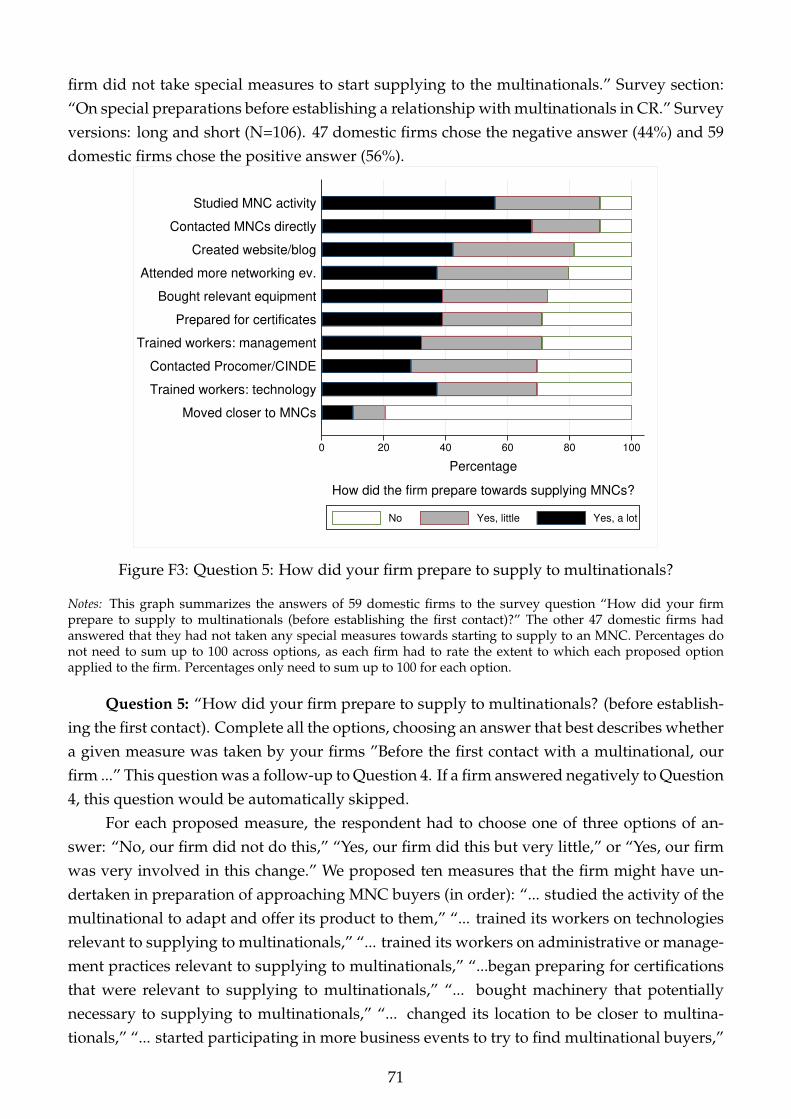
firm did not take special measures to start supplying to the multinationals.” Survey section:“On special preparations before establishing a relationship with multinationals in CR.” Surveyversions: long and short (N=106). 47 domestic firms chose the negative answer (44%) and 59domestic firms chose the positive answer (56%).

0 20 40 60 80 100

Percentage

Moved closer to MNCs

Trained workers: technology

Contacted Procomer/CINDE

Trained workers: management

Prepared for certificates

Bought relevant equipment

Attended more networking ev.

Created website/blog

Contacted MNCs directly

Studied MNC activity

How did the firm prepare towards supplying MNCs?

No Yes, little Yes, a lot

Figure F3: Question 5: How did your firm prepare to supply to multinationals?

Notes: This graph summarizes the answers of 59 domestic firms to the survey question “How did your firmprepare to supply to multinationals (before establishing the first contact)?” The other 47 domestic firms hadanswered that they had not taken any special measures towards starting to supply to an MNC. Percentages donot need to sum up to 100 across options, as each firm had to rate the extent to which each proposed optionapplied to the firm. Percentages only need to sum up to 100 for each option.

Question 5: “How did your firm prepare to supply to multinationals? (before establish-ing the first contact). Complete all the options, choosing an answer that best describes whethera given measure was taken by your firms ”Before the first contact with a multinational, ourfirm ...” This question was a follow-up to Question 4. If a firm answered negatively to Question4, this question would be automatically skipped.

For each proposed measure, the respondent had to choose one of three options of an-swer: “No, our firm did not do this,” “Yes, our firm did this but very little,” or “Yes, our firmwas very involved in this change.” We proposed ten measures that the firm might have un-dertaken in preparation of approaching MNC buyers (in order): “... studied the activity of themultinational to adapt and offer its product to them,” “... trained its workers on technologiesrelevant to supplying to multinationals,” “... trained its workers on administrative or manage-ment practices relevant to supplying to multinationals,” “...began preparing for certificationsthat were relevant to supplying to multinationals,” “... bought machinery that potentiallynecessary to supplying to multinationals,” “... changed its location to be closer to multina-tionals,” “... started participating in more business events to try to find multinational buyers,”

71

“... started contacting multinationals directly, trying to present its products / services,” “...created a website / blog / social networking page to be easier to find by multinationals,” “...approached Procomer / CINDE / MEIC to request assistance in the search for multinationalbuyers.” Figure F3 summarizes the answers to Question 5.

Question 6: “Was there any notable change within your firm just before the first contractwith a multinational that resulted in your firm starting to supply to that multinational? Ifthe answer is YES, provide details about the unexpected event. If the answer is NO, skip tothe next question.” Question type: open-ended. Survey versions: long and short (N=106).100 domestic firms (94%) answered negatively (variations of ”N/A,” ”No,” ”No change”).Six domestic firms (6%) answered positively, offering details on the said change. Here is anexample of one of these positive answers: “Yes, we started advertising our products on a newwebsite and placed ads of the firm in the main search engines.” The described changes do notchallenge the interpretation of our estimates as capturing the treatment effect of becoming asupplier to MNCs.

Question 7: “To your knowledge, did your firm face difficulties in establishing the firstcontracts with multinational buyers? Please choose ONE option only.” Question type: Di-chotomous. Options (in order): “NO, it was relatively easy to start supplying to multinationalbuyers” or “YES, we faced difficulties in trying to start supplying to multinational buyers.”Survey section: “Possible difficulties when trying to establish the first contracts with multi-nationals.” Survey versions: long and short (N=106). 63 domestic firms (59%) provided anegative answer, 43 domestic firms (41%) provided a positive answer.

Question 8: This question was a follow-up to Question 7. If a firm answered negativelyto Question 7, this question would be automatically skipped. Question: “Why was it difficultto get a first contract with a multinational? Consider all the potential answers, indicating howimportant a given explanation was for this difficulty.” Question type: Likert-type scale. Surveyversions: long and short (N=106 surveys, but 43 answers in practice).

For each proposed measure, the respondent had to choose one of four options: “Veryimportant/Crucial,” “Important,” “Perhaps a bit important, not central,” or “Irrelevant.” Weproposed eight potential reasons (in order): Multinationals “were difficult to contact,” “werenot interested in sourcing locally,” “did not know the firm and did not trust the product /service offered,” “expected types of products or services that the firm did not offer,” “expecteda quality of products or services that the firm could not offer at that time,” “required productsor services produced faster than the firm could commit,” “expected lower prices than thosethat this firm could offer,” “required products or services for which the firm had to makelarge investments (for example, buy a machine, expand the scale of production).” Figure F4summarizes the findings from Question 8.

72

0 20 40 60 80 100

Percentage

Required large investment

Not interest. to buy locally

Expected specific inputs

Expected lower prices

Expected higher quality

Expected faster delivery

Difficult to contact

Didn’t know / trust supplier

Why difficult to start supplying to MNCs? MNCs...

Crucial Important Not central Irrelev.

Figure F4: Question 8: Why was it difficult to get a first contract with a multinational?

Notes: This graph summarizes the answers of 43 domestic firms to the survey question “Why was it difficult toget a first contract with a multinational?” The other 63 domestic firms had answered that it was not particularlydifficult to establish a contract with a multinational. Percentages do not need to sum up to 100 across options, aseach firm had to rate the extent to which each proposed option applied to the firm. Percentages only need to sumup to 100 for each option.

Question 9: “What were the changes that the firm experienced when becoming a sup-plier to its first multinational buyers? Select all the answers that are TRUE.” Question type:Multiple-choice. Survey section: “During and immediately after the first contracts with multi-national buyers.” Survey versions: long and short (N=106).

The question allowed for multiple answers among ten options (in order): “The multina-tional firm required specific products or services, so we expanded our portfolio of productsor services that we offered,” “We completely replaced the products or services that we pre-viously offered, with those demanded by multinationals,” “We continued to offer the sameproducts or services, but the quality and / or the price changed,” “We decided to expand ourproductive capacity in order to meet the larger orders from multinationals,” “We hired morehighly qualified workers to help us better serve multinational buyers,” “Our workers had towork harder and longer hours, because the expectations of the multinational were higher thanthey were used to,” “We changed our sourcing strategy (for example, we sourced differentlylocally, imported more),” “We learned from the multinational about management practices ororganization,” “We learned from the multinational about technology relevant for our productsor services.” Figure F5 summarizes the answers to Question 9.

73

0 20 40 60

Percentage

Full replacement ofproduct offer

No change or other

Employees had to work harder

Learning from MNCs on technology

Change in sourcing strategy

Same products, but quality/pricechanged

Hiring of more high−skilledworkers

Expansion of productive capacity

Learning from MNCs on management

Expansion of product scope

Changes for firm upon becoming supplier to first MNC

Figure F5: Question 9: What were the changes that the firm experienced when becoming asupplier to its first MNC buyers? Select all the answers that are TRUE.

Notes: This graph summarizes the answers of 106 domestic firms to the survey question: “What were the changesthat the firm experienced when becoming a supplier to its first multinational buyers? Select all the answers thatare TRUE.” Note that percentages do not need to sum up to 100 across options, as each firm could select alloptions that applied.

Question 10: “Please provide more details about the most important change that thefirm experienced upon becoming a supplier to multinationals.” Question type: Open-ended.Survey section: “During and immediately after the first contracts with multinational buyers.”Survey versions: long and short (N=106). Answers to this question were unguided, hence inorder to be summarized had to be analyzed and grouped by main topic. Table F6 summarizesthe most frequent changes.

Question 11: “How did the first multinational buyers help the firm to undergo thesechanges? Mark all the answers that are TRUE.” Question type: Multiple-choice. Survey sec-tion: “Possible help from the multinational.” Survey versions: long and short (N=106).

The question allowed for multiple answers among nine options (in order): “The multina-tional did not participate directly, did not provide any explicit help, we dealt with the changeson our own,” “The multinational provided a model (”blueprint”) of the desired product orservice or some other relevant documentation,” “Employees of the multinational visited ourfirm and helped us with advice in the adjustment process (for example, the multinational con-ducted audits of the firm and guided it on ways to improve),” “Our employees made visits tothe multinational to observe parts of their production that were relevant to the input we weresupplying to the multinational,” “The multinational had standardized training programs that

74

Table F6: Question 10: What was the most important change experienced upon becoming asupplier to MNCs?

Most Important Change Frequency Percent Cum.

Improved management/organizational practices 24 22.64 22.64Improved product/service quality, 16 15.09 37.74established quality management systemIncreased productive capacity / expansion abroad 13 12.26 50.00No important change 9 8.49 58.49Other 9 8.49 66.98Improved efficiency / delivery times 8 7.55 74.53Improved sourcing / supply chain strategy 8 7.55 82.08Expanded product / service scope 7 6.60 88.68Had to improve firm financing ability 4 3.77 92.45Acquired new machinery / equipment 3 2.83 95.28Improved job security / worker safety 3 2.83 98.11Worked longer hours 2 1.89 100.00

Total N=106 100

Notes: This table summarizes the answers of 106 domestic firms to the survey question: “Please provide moredetails about the most important change that the firm experienced upon becoming a supplier to multinationals.”As this question was open, the team had to organize answers by topic.

they offered to our employees,” “The multinational put us in contact with another firm thatsupplies similar products or services to the multinational in other locations, to advise us onbest practices,” “The multinational has lent us money or paid us in advance so that we canmake the necessary investments,” “The multinational is the one that bought the specific ma-chinery necessary to supply the good / service and they have lent / rented the machinery tous,” “Other: .” Figure F6 summarizes the answers to this question.

75

0 20 40 60

Percentage

MNC paid in advance, helpingsupplier make investments

Other

MNC lent necessary equipmentto supplier

Connected w/ supplier elsewhere,who shared best practices

Training programs foremployees of suppliers

Visits of MNC to supplier: auditsand guidance on improvements

Shared blue print/details of expected product/service

Visits of supplier to MNC to learnabout relevant production processes

No direct/perceived help

What help did first MNC clients provide during adjustment?

Figure F6: Question 11: How did the first MNC buyers help the firm to undergo these changes?

Notes: This graph summarizes the answers of 106 domestic firms to the survey question “How did the firstmultinational buyers help the firm to undergo these changes? Mark all the answers that are TRUE.” Note thatpercentages do not need to sum up to 100 across options.

Question 12: “From the previous answers, please provide more details about the mostimportant assistance provided by the first multinational buyers.” Question type: Open-ended. Survey section: “Possible help from the multinational.” Survey versions: long andshort (N=106).

In the open-ended field, suppliers explained the nature of their interactions with theirfirst MNC buyers and the extent to which these interactions are perceived as help or as in-tegral to their deal. The main takeaway from these answers is that the adjustment periodwas exacting for most local suppliers. While interactions with MNCs were instrumental inunderstanding MNCs’ expectations from both the supplier overall and the product/serviceprovided in particular, these interactions were not always perceived as supportive/helpful.Our interpretation is that during these interactions MNCs placed high demands on their newsuppliers and, while the MNC was constructive in proposing ways to improve, implementingthose suggestions was still in the responsibility of the supplier. For example, the answer ofone domestic form captures the subtle distinction between direct and indirect help:

The most important help received from MNCs came in the form of audits to our plant. Anotherimportant and related support from MNCs was to give us time to address the [quality] complaintsthey made during these audits so that we could develop a business model incorporating their qual-ity standards.

76

Question 13: “If the multinational provided direct/explicit help, how was your firm sup-posed to reward the multinational for this help? Please choose ONE option only.” The questionallowed for a single answer among seven options (in order): “The multinational did not of-fer any (direct/explicit) help in our adjustment to supply it, so this question does not apply,”“The help offered was NOT to be rewarded, it was part of the Corporate Social Responsibilitystrategy of the multinational, there were no specific expectations from the multinational in ex-change of that help,” “The help provided was to be rewarded through lower prices than thosewe could offer before the collaboration with the multinational, for the same product or service(same quality),” “The help provided was to be rewarded through higher-quality products /services, at prices that did not change much,” “The help provided was to be rewarded throughhigher-quality products / services AND ALSO through prices falling,” “The help providedwas to be rewarded through an exclusive contract between our firm and the multinational, wehad to become its exclusive suppliers,” and “Other: .” Survey versions: long and short(N=106). Table F7 summarizes the answers to Question 13.

Table F7: Question 13: If the multinational provided direct/explicit help, how was your firmsupposed to reward the multinational for this help? Please choose ONE option only

Most Important Change Frequency Percent

No direct/explicit help 57 53.77Better quality of product/service, same prices 18 16.98Better quality of product/service, falling prices 12 11.32No need for compensation, part of MNC CSR 11 10.38Lower prices for same product/service quality 4 3.77Other 4 3.77

Total N=106 100

Notes: This table summarizes the answers of 106 domestic firms to the survey question: “If the multinationalprovided direct/explicit help, how was your firm supposed to reward the multinational for this help? Pleasechoose ONE option only”

Question 14: “If your firm has incurred losses from deals with MNC buyers, why doesyour firm have such deals with MNCs, despite this risk of losses? If your firm has never in-curred losses with MNCs, you can skip the question.” Question type: Open-ended. Surveysection: “Possible help from the multinational.” Survey version: long only (N=15). 11 of 15respondents have provided examples of situations when they have incurred losses from dealswith MNCs and their reasons behind tolerating such losses. In general, the answers reflect thestronger bargaining power of MNCs and the longer-term vision of the supplier, who is willingto accept short-term losses with the expectation that the MNC would be satisfied with its ser-vice and continue purchasing its service in the future. The supplier would learn from its initialmistakes and reduce the probability of future losses. Hereafter, we present two examples.

When we started supplying to MNCs, at the very beginning, there was a certain margin of loss.We were expected to be very fast. In the workshop we had to make a lot of efforts. We decided

77

to produce more than what was initially ordered by the MNC, to have a margin in case the MNCordered more. The extra quantities produced and not ordered became losses.

An example from another supplier:

There is uncertainty not in the costs of a given product, but in whether the product will correspondto the expectations [of the MNC buyer]. Given the business of our firm, there is no standardizedproduct. Hence some products might end up costing us more if more iterations are needed. Thefinal product might look very different from what we initially thought. If we make mistakes and donot design the right product from the beginning, this can lead us to a loss. However, we see this asa learning opportunity. Sometimes one has to incur losses to learn.

Question 15: “For a purchase order of the same product, quantity and quality, is therea difference in the price charged to a national buyer with respect to a multinational buyer?Please choose ONE option from the following.” The question allowed for a single answeramong five options (in order): “Almost always a higher price for the multinational buyer,”“More often a higher price for the multinational buyer,” “In most cases, the same price for bothtypes of buyers,” “More frequently, a lower price for the multinational buyer,” and “Almostalways a lower price for the multinational buyer.”

Survey version: only short (N=91.) There was an almost identical question in the longsurvey as well. However, that question was amended to specify that the order was for the samequantity. Suppliers explained during the interviews that for the same product and quality,MNCs are more likely to be offered lower prices as they typically place larger orders. Table F8summarizes the choices made by the 91 domestic firms to Question 15.

Table F8: Question 15: For a purchase order of the same product, quantity and quality, is therea difference in the price charged to a national buyer with respect to a multinational buyer?

Answer Frequency Percent

Usually same price 53 58.24More frequently a lower price for MNC 14 15.38More frequently a higher price for MNC 10 10.99Almost always a higher price for MNC 9 9.89Almost always a lower price for MNC 5 5.49

Total N=91 100

Notes: This table summarizes the answers of 91 domestic firms to the survey question: “For a purchase order ofthe same product, quantity and quality, is there a difference in the price charged to a national buyer with respectto a multinational buyer? Please choose ONE option from the following.”

78

Table F9: Question 16: Has becoming a supplier of MNCs changed your firm’s business withdomestic buyers?

Choices Freq. Percent Details on main reason Freq. Percent

No. No Impact 59 55.66

Yes. Sold More 31 29.25Better quality, same prices 15 48.39Higher visibility 9 29.03Same quality, lower prices 4 12.90Attractive new offer 2 6.45Better quality, even if higher prices 1 3.23

Total N=31 100

Yes. Sold Less 16 15.09Own decision to focus on MNCs 9 56.25Attractive new offer, higher prices 4 25.00New offer not attractive, similar prices 3 18.75

Total N=16 100

Total N=106 100

Notes: This table summarizes the answers of 106 domestic firms to the survey question: “Has becoming a supplierof a multinational changed your firm’s business with domestic buyers? Please choose ONE option only from theoptions below that best describes this impact.”

Question 16: “Has becoming a supplier of a multinational changed your firm’s businesswith domestic buyers? Please choose ONE option only from the options below that best de-scribes this impact.” The question allowed for a single answer among ten options (in order):“No. There was no impact on our domestic business, we continued to sell the same products,at the same prices, without changes in the demand of domestic buyers,” “Yes, in general weDECIDED to sell LESS to domestic buyers, since we decided to focus only on multinationalbuyers,” “Yes, in general we started selling LESS to domestic buyers, because we started pro-ducing goods or services that were not attractive to domestic buyers, despite similar prices,”“Yes, in general we started selling LESS to domestic firms because, despite producing attrac-tive goods or services, these goods or services were too expensive for domestic buyers,” “Yes,in general we started selling MORE to domestic buyers, because we were selling better qualityproducts / services, at the same price as before,” “Yes, in general, we started selling MORE todomestic buyers, because we were selling products / services of the same quality, but at lowerprices than before,” “Yes, in general we started selling MORE to domestic buyers, because we

79

were selling better quality products / services EVEN IF at higher prices than before,” “Yes, ingeneral we started selling MORE to domestic buyers, because we were selling new products orservices than those we offered before,” “Yes, in general we started selling MORE to domesticbuyers, because selling to multinationals made us more visible in the market. However, theproducts and prices had not really changed,” and “Other: .” Survey versions: long andshort (N=106). Section: “Relationships with other types of buyers.”

Table F9 reports the findings from this question. First, we group choices in three broadcategories: “No. No Impact” (option 1), “Yes. Sold Less” (options two to four), and “Yes. SoldMore” (options five to nine). While five firms had originally chosen the “Other: ” option,their answers fell into an already existing option among the previous nine. These broad groupsare reported in decreasing order of frequency. We then provide details on the actual choices offirms falling into either the “Yes. Sold More” or “Yes. Sold Less” categories.

Question 17: “Did becoming a supplier to a first multinational improve the ability ofyour firm to obtain more multinational buyers? Please choose ONE option only.” Questiontype: Dichotomous. Options in order: “NO. Finding each new multinational buyer is as dif-ficult as finding the first multinational buyer” or “YES. Becoming a supplier to a first multi-national improved the capacity of our firm to obtain more multinational buyers.” Survey ver-sions: long and short (N=106). Section: “Relationships with other types of buyers.” 83 do-mestic firms chose the “YES” answer (78%) and 23 domestic firms chose the “NO” answer(22%).

Table F10: Question 18: Why was it easier to find more multinational buyers after having yourfirst (multinational) buyer? Please choose all the options that are TRUE.

Answer Frequency Percentage

Easier to gain MNCs’ trust 71 85.5Learned about MNCs’ needs 60 72.3Improved managerial practices 52 62.7Expanded product/service offer 43 51.8Improved quality without price rise 37 44.6Improved quality with price rise 25 30.1Lowered prices on prior products/services 5 6Other 2 2.4

Notes: This table summarizes the answers of 83 domestic firms to the survey question: “Why was it easier to findmore multinational buyers after having your first (multinational) buyer? Please choose all the options that areTRUE.” Note that the frequency of answers does not need to sum up to 83 or the percentage to 100, as each firmcould select all options that applied.

Question 18: “Why was it easier to find more multinational buyers after having your first(multinational) buyer? Please choose all the options that are TRUE.” Question type: Multiple-

80

choice. Survey section: “About the multinational buyers that followed.” Survey versions:long and short (N=106 surveys, but 83 answers in practice). This question was a follow-up toQuestion 17. If a firm selected the negative answer in Question 17, it would automatically skipthis question. Hence, the following findings pertain to the 83 domestic firms choosing “YES”in Question 17. Table F10 summarizes the answers to Question 18.

Question 19: “How many of the deals of your firm with multinational buyers in CRoccur through Procomer? Please choose ONE option only.” The question allowed for a singleanswer among five options (in order): “(Almost) all deals are mediated through Procomer,”“More than half of the deals are mediated by Procomer, but not all,” “Less than half of the dealsare mediated through Procomer, but there are still many,” “Very few (or almost none) of thesedeals are mediated through Procomer.” Survey version: long only (N=15). Survey section:“On the intermediation of deals with multinationals by Procomer.” Table F11 summarizes theanswers to Question 19.

Table F11: Question 19: How many of the deals of your firm with multinational buyers in CRoccur through Procomer? Please choose ONE option only.

Answer Frequency Percentage

Very few to almost none 12 80.00Less than half, but some 2 13.33(Almost) all 1 6.67

Total N=15 100

Notes: This table summarizes the answers of 15 domestic firms to the survey question: “How many of the dealsof your firm with multinational buyers in CR occur through Procomer? Please choose ONE option only.”

Question 20: “What are the main reasons why your firm wants to make such dealsthrough Procomer? Please, choose (at most) the two most relevant options.” The question al-lowed for at most two answers out of six options (in order): “Procomer deals are not differentfrom the deals we get for ourselves, but allow us to have multiple sources of deals,” “Pro-comer has better access to multinational buyers or the specific type of deals our firm wishes tohave (for example, larger amounts, longer contracts, more high-tech buyers, etc.),” “Procomergives us credibility in front of multinational buyers,” “Procomer prepares us before each spe-cific deal with a multinational buyer, so we feel better prepared to start deals mediated byProcomer,” “Procomer accompanies our deals with multinational buyers, provides us withservices even after the deal was made and is in progress,” and “Other: .” Survey version:long only (N=15). Survey section: “On the intermediation of deals with multinationals byProcomer.” Table F12 summarizes the answers to Question 20.

Question 21: “Please share with us the most negative surprise or the biggest disappoint-ment for your firm after becoming a supplier to MNCs.” Question type: Open-ended. Survey

81

Table F12: Question 20: What are the main reasons why your firm wants to make such dealsthrough Procomer? Please, choose (at most) the two most relevant options.

Answer Frequency Percentage

Procomer has better access to MNCs 9 60.0Deals not different, just another source of deals 8 53.3Procomer offers credibility in front of MNCs 6 40.0Procomer helps prepare the firm before the deals 0 0.0Procomer accompanies the firm during the deals 0 0.0

Other 2 13.3

Notes: This table summarizes the answers of 15 domestic firms to the survey question: “What are the mainreasons why your firm wants to make such deals through Procomer? Please, choose (at most) the two mostrelevant options.”

section: “Questions to wrap up.” Survey version: only long (N=15).The general message is that domestic suppliers often find themselves in asymmetric rela-

tionships with MNCs, where they feel that their efforts to make the relationship successful arenot reciprocated. There is also a significant imbalance of power, size, and financial robustnessbetween MNCs and domestic suppliers to which MNCs do not seem to be sensitive. Hereafter,we include the answers of two different suppliers that are representative of the other answers.

One negative surprise is that MNCs do not seem to understand how impactful some of their mis-takes are for their small suppliers. For instance, MNCs do not seem to be aware of how costly itis for us, as a small firm, to prepare a bid. Therefore they invite us to bid, despite having alreadychosen the winner. Or, sometimes, bills are misplaced, and our payment is made with delay. Evenofficially, MNCs have gone from 15 days of trade credit to up to 120 days. MNCs use the entiretrade credit length agreed upon initially (say 120 days). Once a bill gets to accounting, it will bepaid automatically 120 days after. It is true that the payment is most of the time reliable. But smallsuppliers like us are bearing a lot of the risks and providing financing to MNCs, as opposed to theother way around. This is surprising given how small our bills are compared to the overall turnoverof these MNCs.

We were very hopeful of positive outcomes before the first contracts. However, we had to lowerprices massively to be granted those contracts. MNCs were aggressive in negotiating the reductionof prices. We still have to offer very low rates to maintain these contracts. Also, we started the dealswith MNCs with one month of trade credit. Now, MNCs expect 3.5 months of credit on average.Finally, we feel that MNCs are not very interested in developing local suppliers, that they act as ifthey are entitled to receive high-quality goods or services at meager prices.

Question 22: “Please share with us the most positive surprise or the biggest unexpectedbenefit for your firm after becoming a supplier to MNCs.” Question type: Open-ended. Surveysection: “Questions to wrap up.” Survey version: only long (N=15).

The main takeaway from these answers is that these domestic firms are now enjoying the

82

fruits of their initial hardships experienced upon becoming suppliers to MNCs. The followingis a representative quote from one of the respondents.

The beginnings [of relationships with MNCs] were very tough because we had to lower prices a lot.Once we adapted to the new ways of doing business, we started growing. We started buying newmachines or renovating older machines, having more employees. The hardship at the beginningallowed us to rise afterward. Year after year, the contracts get renewed, so we need to continuelearning and maintaining competitive prices. Whenever the costs of inputs increase, we have toimprove on some other dimension to keep our prices low [better-trained machine operators, fastermachines, etc.]. Also, now the MNCs have become more involved. Sometimes staff from MNCsask: “What is slowing you down? Let us help you with that.”

Online Appendix F.3.2 Survey Answers from Multinational Firms (MNCs)

Question 1: “Country where the headquarters of the multinational is.” Question type:open-ended. Survey versions: long and short (N=58). Responses are summarized in TableF13.

Table F13: Question 1: MNC’s Headquarters Country

HQ country Frequency Percentage

United States 24 41.38Great Britain 4 6.90Costa Rica 3 5.17Germany 3 5.17Netherlands 3 5.17Panama 3 5.17Spain 2 3.45France 2 3.45Japan 2 3.45Venezuela 2 3.45Belgium 1 1.72Canada 1 1.72Switzerland 1 1.72Colombia 1 1.72Guatemala 1 1.72Ireland 1 1.72Cayman Islands 1 1.72Mexico 1 1.72Peru 1 1.72El Salvador 1 1.72

Total N=58 100

Notes: This table summarizes the answers of 58 multinationals to the survey question: “Country where the head-quarters of the multinational is.”

Question 2: “Your position (job title) in the multinational.” Question type: open-ended.Survey versions: long and short (N=58). Responses are summarized in Table F14.

83

Table F14: Summary of Job Titles for Respondents to the Survey to Multinationals

Position (Standardized) Frequency Percentage

Supply Chain/Procurement/Operations Manager 22 37.93General Manager CR Operation / Country Manager 18 31.03Other Unit Manager 14 24.14Supply Chain/Procurement Specialist 4 6.90

Total N=58 100

Notes: This table summarizes the answers of 58 respondents (to the survey to multinationals) to the survey ques-tion: “Your position (job title) in the multinational.” We have grouped job titles under four categories. Under“Supply Chain/Procurement/Operations Manager,” one can find job titles such as Purchasing Manager (“Ger-ente de Compras”), Global Operations Manager (“Gerente Global de Operaciones”), or Purchasing and LogisticsManager (“Gerente de Compras y Logistica”). Under “General Manager CR Operation / Country Manager,” onecan find job titles such as Plant Manager (“Gerente de Planta”), Manager of XX Costa Rica (“Gerente de XX CostaRica”) or Site Supervisor. Under “Other Unit Manager,” one can find job titles such as Manager of Public Rela-tions (“Gerente Asuntos Publicos”), Manager of Government Affairs (“Gerente de Asuntos Gubernamentales”),or Finance Manager (“Gerente Financiero”). Under “Supply Chain/Procurement Specialist,” one can find jobtitles such as Buyer (“Encargado de Compras”) or Import/Export Analyst (“Analista Import / Export”).

Question 3: “To your knowledge, how important were the following factors in the deci-sion of the multinational to locate itself in CR? Complete all the options, choosing how impor-tant you think each criterion was. Note: There is a separate question about the decision to stayand / or expand in CR.” Question type: Likert-type scale. Survey versions: long and short(N=58). Section: “General questions about the multinational’s incentives to invest in CR.”

For each proposed factor, the respondent had to choose one of four options: “Very im-portant/Crucial,” “Important,” “An advantage, but not that important,” or “Not important,does not apply.” We proposed eight potential reasons (in order): “The distance between CRand the HQ country,” “The distance between CR and your target markets,” “The Costa Ricanmarket itself,” “The level of education of the labor force,” “Relatively low wages for the typeof employees needed by the multinational,” “Tax conditions such as the Free Zone regime,”“The availability of suppliers at the prices and / or quality that the multinational needs,” “Thenatural resources (for example, minerals) of CR, necessary for the production of the multina-tional.” Figure F7 summarizes the findings from Question 3.

84

0 20 40 60 80 100

Percentage

Dist. to HQ country

Natural resources

Potential local suppliers

Rel. competitive wages

CR market itself

Dist. to target markets

Education of workforce

Fiscal incentives

Factors affecting MNC decision to come to CR

Critical Important A plus only Irrelev.

Figure F7: Question 3: How Important Were the Following Factors in the Decision of theMultinational to Locate Itself in CR?

Notes: This graph summarizes the answers of 58 multinationals to the survey question “To your knowledge,how important were the following factors in the decision of the multinational to locate itself in CR? Complete allthe options, choosing how important you think each criterion was.” Percentages do not need to sum up to 100across options, as each respondent had to rate the extent to which each criterion had been relevant to the MNC.Percentages only need to sum up to 100 for each criterion.

0 20 40 60 80 100

Percentage

Dist. to HQ country

Natural resources

Potential local suppliers

CR market itself

Rel. competitive wages

Dist. to target markets

Fiscal incentives

Education of workforce

Factors affecting MNC decision to stay and invest more in CR

Critical Important A plus only Irrelev.

Figure F8: Question 4: To your knowledge, how important were the following factors in thedecision of the multinational to STAY or EXPAND in CR?

Notes: This graph summarizes the answers of 58 multinationals to the survey question “To your knowledge, howimportant were the following factors in the decision of the multinational to STAY or EXPAND in CR? Completeall the options and choose how important you think each criterion was.” Percentages do not need to sum up to100 across options, as each respondent had to rate the extent to which each criterion had been relevant to theMNC. Percentages only need to sum up to 100 for each criterion.

85

Question 4: “To your knowledge, how important were the following factors in the de-cision of the multinational to STAY or EXPAND in CR? Complete all the options and choosehow important you think each criterion was.” Question type: Likert-type scale. Survey ver-sions: long and short (N=58). Section: “General questions about the multinational’s incentivesto invest in CR.” The scale and the options were the same as those proposed for Question 3.Figure F8 summarizes the findings from Question 4.

Table F15: Question 5: In general, how important are the following criteria when choosing anew supplier in CR (Costa Rican or not)?

Criterion Critical V. Important Important Only useful Irrelevant

Quality of products/services 74.1 17.2 6.9 0.0 1.7Will or ability to adapt to MNCs 58.6 27.6 10.3 1.7 1.7Price of products/services 43.1 32.8 15.5 6.9 1.7Reliability, traceability etc. 32.8 36.2 19.0 6.9 5.2ISO certificates 22.4 48.3 15.5 5.2 8.6Productive capacity 13.8 29.3 34.5 10.3 12.1Will or ability to invest 10.3 32.8 25.9 13.8 17.2Distance supplier-MNC 6.9 25.9 20.7 25.9 20.7Prior experience exporting 6.9 19.0 15.5 25.9 32.8Foreign language 5.2 20.7 17.2 19 37.9Prior experience w/ MNCs 3.4 36.2 25.9 19 15.5Same HQ country 3.4 1.7 5.2 19.0 70.7Be part of a FTZ 3.4 3.4 13.8 22.4 56.9Will to move closer 1.7 19.0 19.0 36.2 24.1Being foreign-owned 0.0 0.0 1.7 15.5 82.8

Notes: This table summarizes the answers of 58 multinationals to the survey question “In general, how importantare the following criteria when choosing a new supplier in CR (Costa Rican or not)? Complete all the options,selecting the importance that you think each criterion has.” Percentages do not need to sum up to 100 acrosscriteria, as each respondent had to rate the extent to which each criterion is relevant to the MNC. Percentagesonly need to sum up to 100 for each criterion.

Question 5: “In general, how important are the following criteria when choosing a newsupplier in CR (Costa Rican or not)? Complete all the options, selecting the importance thatyou think each criterion has.” Section: “Relations with local suppliers (located in CR). Fromthis moment, our questions will focus on the relationship between the multinational and itslocal suppliers.”

For each proposed factor, the respondent had to choose one of five options: “Of criticalimportance,” “Very important,” “Important,” “Useful, but not a decisive factor,” or “Withoutimportance, irrelevant, does not apply.” We proposed fifteen potential reasons (in order): “Thephysical distance between the supplier and the multinational,” “The willingness of the sup-plier to move closer to the multinational,” “Having previous experience with multinationals,”“Having previous experience exporting,” “Being from the same country as the multinational,”“Being foreign-owned, even if not from the same country as the multinational,” “Being under

86

the Free Trade Zone regime,” “The price of goods or services already on offer,” “The qualityof goods or services already on offer,” “Willingness or ability to adapt and supply the ex-act product or service needed by the multinational,” “Having a manager (or employee) whospeaks the main language of the multinational,” “Reliability / inventory management / inputtraceability / other characteristics of the organization,” “Having standardized quality certifi-cates, relevant to the business (for example, ISO-13485 in the medical device sector),” “Thesize of the supplier, that is, that already has sufficient productive capacity,” “The willingnessor ability to make large investments to supply to the multinational.” Table F15 summarizes theanswers to Question 5.

Question 6: “Does the multinational provide any particular support or guidance to a newsupplier to improve its ability to supply to the multinational?” Question type: Dichotomous.Survey version: both short and long (N=15). Question type: Dichotomous. The two optionsavailable were “NO, the multinational does not provide any explicit support” and “YES, themultinational carries out specific actions to help the new supplier adapt to their relationship.”

40 multinationals answered “YES” (69%) and 18 multinationals answered “NO” (31%).

Table F16: Question 7: Which of the following options describe the way(s) in which the multi-national provides support to the new supplier to adapt to their new relationship?

Support Frequency Percentage

Share blueprint/details of expected product/service 33 82.5Visits of supplier to MNC, learn about relevant production process 33 82.5Visits of MNC to supplier, audits and guidance on improvements 32 80.0Training programs for suppliers’ workers 13 32.5Connect w/ supplier elsewhere, who shares best practices 9 22.5MNC pays in advance, helping supplier make investments 6 15.0MNC lends necessary equipment to supplier 2 5.0Other 5 12.5

Notes: This table summarizes the answers of 40 respondents (to the survey to multinationals) to the surveyquestion: “Which of the following options describe the way(s) in which the multinational provides supportto the new supplier to adapt to their new relationship? Mark all the answers that are TRUE.” Note that the 18multinationals that responded “NO” to Question 6 skipped this question.

Question 7: “Which of the following options describe the way(s) in which the multina-tional provides support to the new supplier to adapt to their new relationship? Mark all theanswers that are TRUE.” Question type: Multiple-choice. Survey section: “More details on thesupport provided by the multinational to suppliers.” Survey versions: long and short (N=40).

We proposed eight potential options (in order): “The multinational provides an instruc-tion manual (”blueprint”) of the desired product or service or other relevant documentation,”“Employees of the multinational visit the supplier and help it with advice in the adjustment

87

process (for example, the multinational performs supplier audits and guides the supplier onways to improve),” “Employees of the supplier are invited to visit the multinational to ob-serve parts of its production that are relevant to the inputs they will supply to the multina-tional,” “The multinational has standardized training programs that the multinational offersto employees of local suppliers,” “The multinational puts the supplier in contact with anothersupplier that sells similar products or services to the multinational in other places, to advisethe new supplier on best practices,” “The multinational lends money or pays the firm in ad-vance so that the firm can make the necessary investments,” “The multinational is the one thatbuys the specific machinery necessary to provide the good / service and lends / rents it to thelocal supplier,” or “Other: .” Table F16 summarizes the answers of 40 multinationals toQuestion 7.

Question 8: “If possible, please provide more details on the most important way in whichthe multinational assists the supplier to adjust to its new relationship with the multinational.For example, the duration of the assistance provided, the frequency of the assistance, the num-ber of trained employees, the size of the loan offered and the conditions, etc.” Question type:Open-ended. Survey section: “More details on the support provided by the multinational tosuppliers.” Survey version: long and short (N=40). This question was a follow-up to Question7, for those having chosen “YES” in Question 6.

Each MNC responding positively to Question 6 provided details on its most importantform of support extended to its new suppliers. The main takeaway is that there is great varietyin the breadth and depth of the support provided by MNCs to their new suppliers. The lighterforms of assistance include sharing of detailed descriptions of the good or service expected(without additional guidance on how to actually produce it) or sharing of an instruction man-ual on the general practices that MNCs expect their suppliers to follow. The following quotepertains to one of the MNCs whose support seemed more substantial.

The most important help that we offer comes in the form of standardized training programs. Giventhat our industry has very high standards of quality, we need to make sure that our suppliers canlive up to the same standards as we do. For that reason, our local experts provide tailored trainingto suppliers, share corporate best practices with them. This leads to a win-win: it benefits us as itturns the supplier into an ally, it benefits the supplier as it is improving its [business and technical]practices. Whether the training is offered only to the manager of the supplier or whether it includesother employees as well depends on the nature of the training, how deep it goes into the processesof the supplier, how large is the gap between where the supplier is and where it needs to get.

Question 9: “How is the supplier expected to compensate the multinational for the sup-port received? Please choose ONE option only.” Survey section: “More details on the supportprovided by the multinational to suppliers.” Survey version: long and short (N=40).

The question allowed for a single answer among seven options (in order): “The supportprovided is NOT intended to be reciprocated. For example, this support is part of the Corpo-rate Social Responsibility strategy of the multinational,” “The support must be correspondedthrough lower prices in the SHORT-TERM than the prices that the firm could offer before thecollaboration with the multinational, for the same product or service,” “The support must be

88

corresponded through a trend of GRADUALLY decreasing prices compared to the prices thatthe firm could offer before the collaboration with the multinational, but for the same prod-uct or service,” “The support must be corresponded through ensuring a higher quality of theproduct / service, BUT with prices that do not change much,” “The support must be corre-sponded through ensuring a greater quality of the product / service AND with prices alsofalling,” “The support must be reciprocated through an exclusivity contract between the firmand the multinational, the firm must become an exclusive supplier,” or “Other: .”

Table F17 summarizes the answers of 40 multinationals to Question 9.

Table F17: Question 9: How is the supplier expected to compensate the multinational for thesupport received? Please choose ONE option only.

Compensation Frequency Percentage

Increasing quality, prices not changing much 15 37.5Increasing quality, falling prices 12 30.0Not to be compensated, part of CSR 8 20.0Other 3 7.5Exclusivity contract b/n MNC and supplier 1 2.5Quickly falling prices, same product/service 1 2.5

Total N=40 100

Notes: This table summarizes the answers of 40 respondents (to the survey to multinationals) to the surveyquestion:“How is the supplier expected to compensate the multinational for the support received? Please chooseONE option only.” Note that the 18 multinationals that responded “NO” to Question 6 skipped this question.

Question 10: “Please, if possible, provide more details about the previous answer.” Thisquestion is a follow-up to the question above. Survey section: “More details on the supportprovided by the multinational to suppliers.” Survey version: long only (N=23).

By and large, MNC staff describe the support provided to the suppliers of the MNC asmeant to establish a win-win collaboration. The following answer from the Supply ChainManager of one MNC is representative for all other 22 answers.

While there is no formal commitment during the period of support, we expect that the supplier iswilling to educate itself, to learn how to improve the quality and service offered. Moreover, we helpthe supplier improve its processes, its management practices. Hence there is the expectation thatcost reductions would be shared between the supplier and us, that the help we provided led to awin-win situation. For instance, we excel in lean manufacturing and invite suppliers to see how wemanage our operation, so that they can apply the same principles to their operation. Suppliers areunder constant control of their quality and service. If we put suppliers under probation and if theirquality/service does not improve within a couple of months, they lose the contract with us.

Questions 11, 12, and 13: We summarize here the answers to three consecutiveand related questions: “From your point of view, what are the three most probable prof-

89

its/benefits/advantages that Costa Rican firms experience when they become suppliers ofMNCs? Provide details to your answers.” All three answers were open-ended. Surveyversion: long only (N=23). In Table F18 we categorized the answers provided by the 23respondents into four categories, which we created based on the common themes emergingacross answers.

Table F18: Questions 11, 12, and 13: Top three most important benefits to becoming a supplierto MNCs, according to MNCs

Most important benefit Second most important benefit Third most important benefit

9 Stability and predictability 11 Learning opportunities 12 Learning opportunities7 Learning opportunities 7 Stability and predictability 5 Scale and global opportunities6 Scale and global opportunities 4 Scale and global opportunities 2 Stability and predictability1 Reputation 1 Reputation 1 Reputation0 None 0 None 3 None

N=23 N=23 N=20

Hereafter, we provide an example of an answer for each of the four categories. Eachanswer comes from a different respondent.

Example for “stability and predictability”:

The first most important gain/benefit /advantage for Costa Rican firms is the contract length. Thetype of business they establish is a win-win relationship, where it is possible for suppliers to projectthemselves into the future and begin to be part of a stable supply chain.

Example for “learning opportunities”:

The third largest gain/benefit/advantage derived from becoming a supplier to MNCs has to dowith the improvements and the strengthening of the management model of the supplier, both con-cerning production and service provision. The modus operandi a supplier learns during the col-laboration with MNCs is helpful in several ways. If the supplier manages to standardize processesand apply the same principles for other clients, the supplier will always win because it is betterprepared. This gain is particularly significant for SMEs.

Example for “scale and global opportunities”:

Once a firm joins our list of approved suppliers for a given commodity, opportunities are globalfor that supplier within the organization. [They] are in the system and visible globally. That sup-plier becomes available to anyone at any site. As long as the pricing is correct and the businessproposition is the right one, then they can supply elsewhere as well.

Example for “reputation”:

The second largest gain goes to the reputation of the supplier. Once one MNC uses a supplier, giventhe high expectations of MNCs, if that initial deal goes well, the news spreads to other MNCs thathave similar requirements.

Questions 14, 15, and 16: We summarize here the answers to three consecutive andrelated questions: “From your point of view, what are the three losses/risks/disadvantages

90

that Costa Rican companies experience when they become suppliers of MNCs? Provide detailsto your answers.” All three answers were open-ended. Survey version: long only (N=23).

In Table F19 we categorized the answers provided by the 23 respondents into six cate-gories, which we created based on the common themes emerging across answers.

Table F19: Questions 14, 15, and 16: Top three most important risks to becoming a supplier toMNCs, according to MNCs

Most important risk Second most important risk Third most important risk

11 Financial or legal risk 7 None 18 None7 Demanding changes 5 Demanding changes 2 Financial or legal risk3 None 4 Financial or legal risk 1 Bad reputation1 Bad reputation 4 Bad reputation 1 Demanding changes1 Specificity 2 Other 1 Other0 Other 1 Specificity 0 Specificity

N=23 N=23 N=23

Hereafter, we provide an example of an answer for the categories “financial or legal risk,”“demanding changes,” “bad reputation,” and “specificity.” Each answer comes from a differ-ent respondent.

Example for “financial or legal risk”:

A first considerable risk comes from the volumes ordered by MNCs. The supplier might need to in-vest a lot to live up to its large orders. However, if the supplier is unable to deliver the expected levelof quality and service, it might lose the contract and get in trouble because of the investment made.It is not the policy of the multinational to sign long-term contracts with a supplier because theycannot commit to continuing a contract with a supplier that does not deliver what it is supposed todeliver time and again.

Example for “demanding changes”:

The most significant disadvantage/risk has to do with the level of pressure that a firm is put underwhen becoming a supplier to an MNC. Supplying to an MNC comes with many requirements, manyspecifications, high standards. MNCs are very demanding. This can be very stressful for a smallCosta Rican firm. Sometimes some misunderstandings come up due to misaligned expectations.

Example for “bad reputation”:

The second most important risk is reputational. MNCs participate at seminars, at fora. They ex-change on their experience with local suppliers. If a given relationship with an MNC goes sour,then this will become quickly known to other MNCs as well. For this reason, every commercial re-lationship matters for the reputation of a supplier, not to gain a reputation of being a bad supplier,from which it is hard to recover.

Example for “specificity”:

91

Given the market in which the MNC is, suppliers of direct inputs might feel too narrowly special-ized.

Questions 17 and 18: We bundle together these two questions. Question 17 asked aboutthe procurement decision process on key inputs, Question 18 about the decision process on sec-ondary inputs. “WHICH AFFILIATE decides on the procurement of KEY (or SECONDARY)INPUTS for the affiliate in CR and HOW? Please choose ONE option only. Note: Key inputsare those inputs that affect the quality and final characteristics of the core product. An exam-ple of a good / service that may not be key (may be secondary) is packaging or spare parts forthe machinery used in production.”

The question allowed for a single answer among six options (in order): “Most decisionsabout key (secondary) inputs are made by the headquarters (or another affiliate other thanthe affiliate in CR), with little to no feedback on Costa Rican suppliers from the Costa Ricanaffiliate,” “Most of the decisions on key (secondary) inputs are made by the headquarters (oranother affiliate other than the affiliate in CR), but with comments on Costa Rican suppliersfrom the Costa Rican affiliate,” “Decisions on key (secondary) inputs are made jointly betweenthe headquarters (or another affiliate other than the affiliate in CR) and the Costa Rican sub-sidiary,” “Most decisions on key (secondary) inputs are made by the Costa Rican affiliate, butwith comments from the headquarters (or another affiliate other than the affiliate in CR),”“Most decisions on key (secondary) inputs are made by the Costa Rican affiliate, with little tono feedback from the headquarters (or any affiliate other than the affiliate in CR),” or “Other:

.” Table F20 summarizes the answers from both Questions 17 and 18.

Table F20: Questions 17 and 18: WHICH AFFILIATE decides on the procurement of KEY(SECONDARY) INPUTS for the affiliate in CR and HOW? Please choose ONE option only.

Core inputs Secondary inputsFrequency Percent Frequency Percent

HQ, little local feedback 7 12.1 0 0.0HQ, with local feedback 12 20.7 3 5.2Joint decision 15 25.9 10 17.2Local, with HQ feedback 8 13.8 14 24.1Local, little HQ feedback 12 20.7 28 48.3Other 4 6.9 3 5.2

Total N=58 100 N=58 100

Notes: This table summarizes the answers of 58 respondents (to the survey to multinationals) to the surveyquestions: “WHICH AFFILIATE decides on the procurement of KEY (SECONDARY) INPUTS for the affiliatein CR and HOW? Please choose ONE option only.”

92

Appendices ReferencesAlberto Abadie and Guido W Imbens. Large Sample Properties of Matching Estimators for Average

Treatment Effects. Econometrica, 74(1):235–267, 2006.

Alberto Abadie and Guido W Imbens. On the Failure of the Bootstrap for Matching Estimators.Econometrica, 76(6):1537–1557, 2008.

Asya Akhlaque, Ong Lopez, Anne Beline Chua, and Antoine Coste. Vietnam - Enhancing EnterpriseCompetitiveness and SME Linkages: Lessons from International and National Experience. WorldBank Working Paper 119861, 2017.

Alonso Alfaro-Urena, Mariany Fuentes, Isabela Manelici, and Jose Vasquez. The Costa Rican Produc-tion Network: Stylized Facts. Research Paper Series, 2018.

Alonso Alfaro-Urena, Isabela Manelici, and Jose Vasquez. The Effects of Multinationals on Workers:Evidence from Costa Rica. Working Paper, 2019.

Pol Antras and Stephen R Yeaple. Multinational Firms and the Structure of International Trade, vol-ume 4, pages 55–130. Elsevier, 2014.

Anne Brockmeyer, Spencer Smith, Marco Hernandez, and Stewart Kettle. Casting a Wider Tax Net:Experimental Evidence from Costa Rica. American Economic Journal: Economic Policy, 11(3):55–87,2019.

Jan De Loecker and Frederic Warzynski. Markups and Firm-Level Export Status. American EconomicReview, 102(6):2437–71, May 2012.

Tatyana Deryugina, Alexander MacKay, and Julian Reif. The Long-Run Dynamics of Electricity De-mand: Evidence from Municipal Aggregation. American Economic Journal: Applied Economics, 12(1):86–114, 2020.

ILO. Women and Men in the Informal Economy: A Statistical Picture. Third Edition. InternationalLabour Office Technical Report, 2018.

S, ebnem Kalemli-Ozcan, Bent Sørensen, Carolina Villegas-Sanchez, Vadym Volosovych, and SevcanYesiltas. How to Construct Nationally Representative Firm Level Data from the ORBIS GlobalDatabase. Note, 2015.

Ricardo Monge-Gonzalez and Juan Antonio Rodriguez-Alvarez. Impact Evaluation of Innovation andLinkage Development Programs in Costa Rica: The Cases of PROPYME and CR Provee. IDB WorkingPaper Series, 461:1–78, 2013.

OECD. Tax Policy Reviews: Kazakhstan 2017. Technical report, OECD, 2017a.

OECD. Tax Policy Reviews: Costa Rica 2017. Technical report, OECD, 2017b.

OECD. Tax Administration 2019. OECD Publishing, Paris, 2019.

Dimitris N Politis and Joseph P Romano. Large Sample Confidence Regions Based on Subsamplesunder Minimal Assumptions. The Annals of Statistics, pages 2031–2050, 1994.

Gabriel Ulyssea. Informality: Causes and Consequences for Development. Annual Review ofEconomics, 12, 2020.

93