1

The Effects of Mandatory Transparency in Financial Market Design:

Evidence from the Corporate Bond Market1

Paul Asquith Thomas R. Covert Parag A. Pathak2

This draft: April 4, 2019

Abstract. In July 2002, FINRA began mandatory dissemination of price and volume information for

corporate bond trades. This paper, using recently released data, measures transparency’s effect on

trading activity and costs for the entire corporate bond market. Even though trading costs decrease

significantly across all types of bonds, trading activity does not increase and, by one measure, decreases.

Transparency affects the high-yield market differently than the investment grade market since high-

yield bonds have the largest decrease in trading activity, 71.1%, and the largest decrease in trading

costs, 22.9%. High-yield bonds also disproportionately contribute to the reduction in estimated trading

costs of $600 million a year.

1 We are grateful to Hank Bessembinder, Edith Hotchkiss, Leonid Kogan, Deborah Lucas, Jun Pan, and Alp Simsek for discussions, and Ola Persson and FINRA for conversations about the data. We also thank Jane Choi, Abhishek Dev, Daniel Green, Joseph Shayani, Josh Weiss, and Ahmad Zia Wahdat for their research assistance. 2 Asquith: MIT Sloan School of Management, Cambridge, MA 02142 and NBER, email: pasquith@mit.edu; Covert: Chicago Booth School of Business, Chicago, IL 60637, email: Thomas.Covert@ChicagoBooth.edu; Pathak: MIT Economics, Cambridge, MA 02142 and NBER, email: ppathak@mit.edu.

2

I. Introduction

Many financial markets have recently become subject to new regulations requiring

transparency. This paper studies how transparency affects trading in the US corporate bond market. In

July 2002, FINRA began requiring the timely public dissemination of post-trade price and volume

information for the $4.4 trillion-a-year U.S. corporate bond market through TRACE (FINRA’s Trade

Reporting and Compliance Engine). Dissemination took place in Phases over two-and-a-half years.

Actively traded, investment grade bonds became transparent before thinly traded, high-yield bonds.

TRACE has become the template for increased transparency in other over-the-counter financial

markets.3 The increase in information due to TRACE was so significant that it has been likened to the

early 20th century introduction of stock market tickers for equities and electronic screens for Treasuries

(Vames 2003).

When market participants have timely information about transaction prices and quantities, it

may lower search costs and alter bargaining between customers and dealers. Several models suggest

that post-trade transparency reduces trading costs and improve market performance. In Duffie,

Garleanu, and Pedersen (2005)’s search-and-matching model, bid-ask spreads decrease when investors

have greater bargaining power. In models with information differences, a reduction in information

asymmetries also reduces transaction costs (e.g., Glosten and Milgrom 1985). FINRA’s (then NASD)

stated rationale for TRACE emphasized that more information would level the playing field between

institutional and retail market participants. TRACE proponents anticipated that everyone, including

dealers, would benefit from increased market participation. For instance, SEC commissioner Arthur

Levitt (1999) remarked, “This participation means more trading, more market liquidity, and perhaps

even new business for bond dealers.”

In this paper, we use previously unreleased data to examine the effects of TRACE on trading

activity and costs over all four Phases of its introduction. The new data includes anonymized dealer

identifiers. These identifiers allow us to directly measure trading costs by measuring the cost of round-

trip trades for all bonds. The data also include transaction information on bond trades that were

collected by TRACE, but not publicly disseminated. The non-disseminated trades allow us to exploit

TRACE’s four distinct Phases to estimate difference-in-differences models of TRACE’s effect. This

provides complete coverage across all segments of the bond market for the first time. In addition, our

research design, which exploits the introduction of TRACE in Phases, isolates the effect of transparency

from other elements of market design since bonds continued to be traded over-the-counter in a dealer

market afterwards.

3 Title VII of the Dodd-Frank Wall Street Reform and Consumer Protection Act (Dodd-Frank) (2010) required that swaps (including credit default swaps, interest rate swaps, collateralized debt obligations, and other derivatives) adopt TRACE-like post-trade transparency beginning in 2011. In addition, FINRA has expanded TRACE to several other asset classes, including Agency-Backed Securities, Asset-Backed Securities, and 144a bonds. TRACE was expanded in March 2010 to include Agency-Backed Securities and in May 2011 to include Asset-Backed Securities. FINRA started publicly disseminating 144A transactions on June 30, 2014. European MiFID II/R regulations mimic TRACE for European corporate bonds and were implemented starting January 3, 2018.

3

Bonds differ substantially between the Phases as does trading activity and trading costs. For

example, bonds in the last Phase (3B) are far more likely to be lower rated high yield bonds than bonds

in the first two Phases (1 and 2), which are all investment grade. In addition, bonds in Phase 3B trade

less frequently than bonds in Phases 1, 2, and 3A. At the same time, Phase 3B bonds have the largest

average trade size and the highest trading-cost per round-trip trade.

These differences in bonds across Phases allow us to show that TRACE has significantly different

effects on the investment-grade and high-yield segments of the bond market. Using a difference-in-

differences methodology, we find that TRACE results in an 11.7% reduction in the number of trades

overall. 4 This result is driven by Phase 3B bonds. TRACE significantly reduces the number of Phase 3B

trades by 71.1% from the mean number of trades prior to dissemination.5 These findings are robust

across variations of our difference-in-differences research design.

TRACE does not significantly change trading volume for any Phase, however. Even though the

number of trades for Phase 3B bonds decrease, TRACE increases the average trade size for Phase 3B

bonds significantly increases by 4.3% or $50,101. Moreover, the reduction in the number of trades in

Phase 3B is driven by trades less than 100,000. These are exactly the small retail trades that proponents

of TRACE predicted would increase the most, yet the data show that they decrease the most.

There is no effect on trading volume even though TRACE reduces round-trip trading costs

significantly in each Phase. A round-trip trade is one where a given quantity of a bond is bought and sold

by the same dealer within a certain amount of time. There is a reduction in round-trip trading costs,

both by trade and by bond traded for each Phase. TRACE reduces round-trip trading costs across all

Phases by 18.5% per round-trip trade and 4.9% per round-trip bond traded. The effects on trading costs

are largest, at 22.9% per round-trip trade and 10.9% per round-trip bond traded, for Phase 3B bonds.

These significant effects are present even though Phase 3B occurs more than two-and-a-half years

following the introduction of transparency in segment of the bond market.

We also investigate differences between dealer and customer trading. We divide round-trip

trades between those with a customer on both ends and a dealer in between (“CDC”), which we refer to

as customer round trips, and those with no customers (“DDD”), which we refer to as dealer round trips.

The customer trading cost per round-trip trade is larger than for dealers at $2,562 for CDCs versus

$1,035 for DDDs. This fact is consistent with dealers having market power or more information than

customers. TRACE has the largest negative effect on customer round-trip trades, and reduces the

dealer cost advantage, but it does not eliminate it. There is a significant reduction in trading cost per

round-trip trade of $454 for CDCs and a $225 for DDDs. On a percentage basis, however, these effects

are similar, showing that TRACE does not level the playing field between customers and dealers.

4 Since there is no systematic data on corporate bond trading prior to TRACE’s introduction, we cannot use our research design to study Phase 1. Following Bessembinder, et. al. (2005), we use data from the National Association of Insurance Commissioners together with our difference-in-differences research design to measure Phase 1 effects on trading activity and costs. Appendix A details these results.

4

Finally, we estimate that the aggregate reduction in trading costs across all Phases is $605

million per year. We also estimate TRACE’s effect on trading revenues per dealer and find that dealer’s

revenue dropped approximately by $695 million a year from transparency. Moreover, the high-yield and

infrequently traded bonds in Phase 3B account for 21.8% of the reduction in trading cost per round-trip

trade and 34.4% of the reduction in dealer revenues, even though they represent only 5.1% of the

trades.

Our results extend the existing literature on TRACE, written before it was fully implemented.

Bessembinder, Maxwell, and Venkataraman (2006), focusing on Phase 1 only, which covered investment

grade and large issue bonds, and using data from the National Association of Insurance Commissioners

(but not TRACE), document a reduction in trade execution costs, estimated using a structural model.

Edwards, Harris, and Piwowar (2007) and Hotchkiss, Goldstein, and Sirri (2007) both using investment-

grade bonds in Phase 2 TRACE data report no effect on trading activity and a decline in transaction costs.

None of these studies consider the last two Phases of TRACE, which cover primarily smaller issue

size bonds and high-yield bonds. Bonds in these segments trade less frequently and were the subject of

the most vocal concerns of TRACE opponents. It was because of these concerns that FINRA phased-in

TRACE over four Phases, and even delayed disseminating certain transactions in the last Phase of TRACE.

Prior work has also focused on model-based estimates of trading costs or reported round-trip measures

of trading costs for small subsamples of bonds. These estimates may not be representative of TRACE’s

overall impact.

The rest of this paper is organized as follows. Section 2 presents additional background on

TRACE and reviews the related literature. Section 3 describes the Academic TRACE database and

presents descriptive statistics. Section 4 describes our research design. Section 5 reports on trading

activity, while Section 6 reports on trading costs. Section 7 investigates trade sizes and trading partner

(either dealer or customers). Section 8 examines dealer revenue and the aggregate effect of TRACE. The

last section states our conclusions and discusses the implications of our findings.

II. TRACE and the Corporate Bond Market II.A History and Implementation of TRACE

The Trade Reporting and Compliance Engine (TRACE) was launched in July 2002, but it has its

origins in the late 1990s when the Securities and Exchange Commission (SEC) reviewed issues related to

price transparency in U.S. debt markets. After this review, the SEC asked the National Association of

Security Dealers (NASD) to take three steps to enhance the transparency and integrity of the corporate

debt market: 1) adopt rules to report all transactions in U.S. corporate bonds to NASD and develop

systems to receive and distribute transaction prices on an immediate basis; 2) create a database of

transactions in corporate bonds to enable NASD and other regulators to take a proactive role in

supervising the corporate debt market; and 3) create a surveillance program to better detect

5

misconduct and foster investor confidence in the corporate debt market. NASD changed its name to the

Financial Industry Regulatory Authority (FINRA) in 2007.6

The SEC and NASD’s stated rationale was to level the playing between institutional and retail

participants in the corporate bond market. Advocates of transparency claimed that almost everyone,

including dealers, would benefit because of increased market participation. As mentioned above, SEC

commissioner Arthur Levitt (1999) remarked, “This participation means more trading, more market

liquidity, and perhaps even new business for bond dealers.”

The anticipated benefits of TRACE and the absence of harm contrasts sharply with the opinions

of many market participants. TRACE opponents argued that “transparency would add little or no value”

to highly liquid and investment grade bonds since these issues often trade based on widely known US

Treasury benchmarks (NASD 2006). Furthermore, the Bond Market Association warned that there

would be negative effects for lower-rated and less frequently traded bonds (Mullen 2004). Dealers may

be less willing to hold inventory because bid-ask spreads subsidize holding costs and TRACE may reduce

these spreads, particularly for less frequently traded securities. Moreover, opponents saw TRACE as

imposing heavy compliance costs, particularly for small firms (Jamieson 2006). Lastly, there was a

concern that dealers who buy large quantities may be particularly disadvantaged since dissemination

would affect the resale price. Not surprisingly, similar arguments for and against transparency

resurfaced in response to the introduction of the Dodd-Frank’s post-trade transparency requirements

for swaps (Economist 2011).

By January 2001, the SEC approved rules requiring NASD members to report all over-the-counter

(OTC) market transactions in eligible fixed income securities to the NASD and mandating that certain

market transactions be disseminated. NASD developed a platform, TRACE, to facilitate this mandatory

reporting. The rules, referred to as the "TRACE Rules," are contained in the new Rule 6200 Series that

replaced the old Rule 6200 Series, which governed the Fixed Income Pricing System (FIPS). FIPS, which

reported transactions information on approximately 50 high-yield bonds, started in April 1994.

On July 1, 2002, FINRA implemented TRACE, requiring dealers to report all bond transactions on

TRACE-eligible securities within 75 minutes. As described in Table 1, FINRA began disseminating price

and volume data for trades in selected investment-grade bonds with an initial issue of $1 billion or

greater (i.e., Phase 1 bonds). FINRA’s dissemination occurred immediately upon reporting for these

bonds. FINRA censored trade size reports at $1,000,000 for high-yield bonds and $5,000,000 for

investment grade bonds, due to the concerns about TRACE’s impact on large trades discussed above

(Vames 2003).7

6 http://www.finra.org/Industry/Compliance/MarketTransparency/TRACE/FAQ/P085430, Last accessed: July 14, 2012. 7 Duffie (2012) states that censoring trade information may “reduce inventory imbalances stemming from large trades with less concern that the size of a trade or their reservation price will be used to the bargaining advantage of their next counterparties.”

6

A “TRACE-eligible security” is any US dollar-denominated debt security that is depository-eligible

and registered by the SEC, or issued pursuant to Section 4(2) of the Securities Act of 1933 and purchased

or sold pursuant to Rule 144a.8 Additionally, the 50 high-yield securities disseminated under FIPS were

transferred to TRACE, which now disseminated their trades.9 We denote these bonds as the FINRA50.

520 securities had their information disseminated by the end of 2002.

At the start of Phase 1, it was not certain when and to what extent TRACE would be expanded.

After all, the FIPS program had existed without expansion for eight years. Initially, a bond transactions

reporting committee comprised of NASD and the Bond Market Association members was established to

study TRACE’s impact. Their mandate was to focus not on the largest, highest quality credit and actively

traded issues, but rather on the rest of the market (Vames 2003). Their recommendation was to expand

TRACE’s coverage. The NASD approved the expansion of TRACE on November 21, 2002 and the SEC

approved it on February 28, 2003.

Phase 2 of TRACE was implemented on March 3, 2003, and it expanded dissemination to include

smaller investment grade issues. The new dissemination requirements included securities with at least

$100 million par value or greater and ratings of A- or higher. In addition, dissemination began on April

14, 2003 for a group of 120 Investment-Grade securities rated BBB. We denote these BBB bonds as the

FINRA120. 10 After Phase 2 was implemented, the number of disseminated bonds increased to

approximately 4,650 bonds.11

Finally, on April 22, 2004, after TRACE had been in effect for some bonds for almost two years,

the NASD approved the expansion of TRACE to almost all bonds. The last Phase came in two parts,

which FINRA designates as Phase 3A and Phase 3B. The distinction between Phase 3A and 3B was in

response to concerns about the adverse effects of immediately disseminating information on large

trades. Phase 3B bonds are eligible for delayed dissemination. Specifically, Rule 6250(b)(2)(A) states

that transactions greater than $1 million on BB bonds that trade an average of less than one time per

day will be disseminated two business days from the time of execution. Rule 6250(b)(2)(B) states that

transactions greater than $1 million on bonds rated B or lower that trade an average of less than one

8 The list of eligible security types is: (1) Investment-grade debt, including Rule 144A/DTCC eligible securities, (2) High-yield and unrated debt of U.S. companies and foreign private companies, (3) Medium-term notes, (4) Convertible debt and other equity-linked corporate debt not listed on a national securities exchange, (5) Capital trust securities, (6) Equipment trust securities, (7) Floating rate notes, (8) Global bonds issued by U.S. companies and foreign private companies, and (9) Risk-linked debt securities (e.g., “catastrophe bonds”). TRACE-eligible securities exclude debt that is not depository-eligible, sovereign debt, development bank debt, mortgage- and asset-backed securities, collateralized mortgage obligations, and money market instruments. 9 Alexander, Edwards, and Ferri (2000) examine the liquidity of the bonds in the FIPS dataset. 10 The FINRA120 sample was selected by FINRA to study the impact of dissemination on market behavior and has been studied by Goldstein, Hotchkiss, and Sirri (2007). 11The FINRA50 subset did not remain constant over our time period. On July 13, 2003, the FINRA50 list was updated, and the list was then updated quarterly for the next 5 quarters. The FINRA50 list was updated on July 13, 2003, October 15, 2003, January 15, 2004, April 14, 2004, and July 14, 2004.

7

time per day will be disseminated four business days from the time of execution.12 TRACE eliminated

delayed dissemination on January 9, 2006.

In Phase 3A, effective on October 1, 2004, 9,558 new bonds started having their trade

information disseminated. In Phase 3B, effective on February 7, 2005, an additional 3,016 bonds started

dissemination, though sometimes with delay. According to the NASD at that point, there was “real-time

dissemination of transaction and price data for 99 percent of corporate bond trades” (NASD 2005).

In an effort parallel to increasing the number of bonds with disseminated trade information,

FINRA began reporting transactions (except for delayed disseminations discussed above) more quickly:

the time-lag between the dealer’s report to FINRA and its public release was reduced from 75 minutes

on July 1, 2002, to 45 minutes on October 1, 2003, to 30 minutes on October 1, 2004, and to 15 minutes

on July 1, 2005. On January 9, 2006, the same day that delayed dissemination was eliminated, the time-

lag for public release was eliminated and trades were disseminated immediately.

II.B Related Literature

There are three early studies of TRACE which focus on Phase 1 or Phase 2. The first,

Bessembinder, Maxwell, and Venkataraman (2006), studies the impact of Phase 1 of TRACE using the

National Association of Insurance Commissioners (NAIC) database, before and after the start of Phase 1.

That database contains insurance company transactions of corporate bonds. Bessembinder et al.

estimate a structural model in which changes in bond prices are regressed on customer buy/sell

dummies and other factors to estimate trade execution costs. They estimate a 4.9-7.9 basis point

reduction in trade execution costs for Phase 1 bonds in a before-and-after comparison. They also

estimate that after Phase 1, transaction costs for bonds not covered in Phase 1 decline by 3.5 basis

points, and that there is a decline in the share of trading activity performed by the 12 largest dealers. In

light of the decline in trade execution costs for non-Phase 1 bonds, they argue that the implementation

of TRACE on the large and high credit quality bonds in Phase 1 had spillover effects on other bonds

whose trades were not disseminated.

Two other studies examine transaction costs for Phase 2 bonds. Edwards, Harris, and Piwowar

(2007) estimate imputed transaction costs using a structural model, similar to the one used in

Bessembinder et al. They find that disseminated bonds have lower estimated transaction costs. Since

this result may be due to bond characteristics rather than the effect of transparency, they also report a

difference-in-differences analysis, which compares the transaction costs of bonds which are newly

disseminated to three distinct control groups of bonds that do not change dissemination status. The

transaction costs of newly disseminated bonds decrease relative to each control group across the entire

12 In addition, dissemination is delayed for the first two days for newly issued BBB rated TRACE-eligible securities for trades that are executed in the first two days after pricing (all trades for the first two days are reported on the third day). Similarly, dissemination is delayed for the first ten days for newly issued BB or lower rated TRACE-eligible securities for trades that are executed in the first ten days after pricing (all trades for the first ten days are reported on the eleventh). Note our sample is restricted to bonds that trade at least 90 days before the start of any Phase and therefore these types of delayed dissemination are not present in our sample.

8

range of trade sizes. Both Bessembinder et al. and Edwards et al. estimate that investors could have

saved a minimum of $1 billion per year if trades were transparent.

Hotchkiss, Goldstein, and Sirri (2007) report on a controlled experiment, commissioned by the

NASD, of 120 BBB bonds, 90 of which are actively traded and 30 of which are relatively inactive. Through

cooperation with the NASD, they construct a matched sample of the 90 actively traded bonds based on

industry, average trades per day, bond age, and time to maturity. When the 90 actively traded bonds

were disseminated on April 14, 2003, the matched bond was not. To increase power, they also compare

the disseminated sample to a larger portfolio of non-disseminated bonds. For the 90 actively traded

bonds, they find declines in transaction costs for all but the group with the smallest trade size. There is

no evidence of a reduction in transaction costs for inactively traded bonds. In subsequent work,

Goldstein and Hotchkiss (2012) study new issues of corporate bonds, and find a secular decline in price

dispersion, measured as the difference between high and low prices charged by the same dealer on the

same day, from July 2002 through February 2007, for newly issued bonds. This fall in price dispersion

does not, however, coincide with the start of any of the TRACE phases.

While these studies provide evidence that TRACE reduces transaction costs for Phase 1 and

Phase 2 bonds, there is little evidence about actual reductions in trading costs and no evidence about

TRACE’s effect on trading activity or trading costs in Phases 3A or 3B. These last two Phases cover

13,940 bonds (or 82.7% of all bonds) and 55.7% of trading activity from July 2002 – December 2006. The

SEC, and others, saw the evidence above as inconclusive, stating that concerns about liquidity were not

rejected.13 Duffie (2012) concludes “the empirical evidence does not generally support prior concerns

by dealers that the introduction of TRACE would reduce market liquidity.” More recently, Dugalic

(2017) studies the behavior of core and peripheral dealers in the period surrounding the introduction of

TRACE. Following our research design, he finds that transparency influences trading between the core

and peripheral dealers.

The absence of any adverse effect on trading activity is surprising considering the negative

reaction to TRACE from many market participants. For instance, Bessembinder and Maxwell (2008)

survey dealers and report that bond dealers almost universally perceive that trading became more

difficult after TRACE. (See also Jamieson 2006 and Decker 2007).14 This may be a consequence of the

earlier studies’ focus on Phase 1 and Phase 2 since our paper finds a reduction in trading activity for

bonds in Phase 3B.

13 The SEC’s Director of Market Regulation Nazareth (2004) stated “the NASD commissioned two studies to address this issue [the impact of TRACE on liquidity]. Neither study provided significant evidence that transparency harms liquidity. However, neither study was extensive enough to address all concerns raised by dealers and other market participants.” The industry group, the Bond Market Association, described these studies as largely inconclusive (Mullen 2004). 14 Bessembinder and Maxwell (2008) are skeptical of these claims given that there was an upward trend in aggregate corporate bond trading from 2002-2007. This increase in aggregate bond trading does not imply TRACE increased trading activity, however, since there was also an upward trend in the amount of corporate debt outstanding due to new issues. When we hold the number of bonds constant by examining bonds newly disseminated in TRACE’s four Phases, there is a downward trend in the number of trades (see Figure 1).

9

A set of studies on municipal bonds is also relevant to the TRACE experiment. On January 31,

2005, the Municipal Securities Rulemaking Board (MSRB) started requiring that information about

trades in municipal bonds be reported within 15 minutes, similar to TRACE. Prior to that dissemination,

Green, Hollifield, and Schurhoff (2007a) find significant price dispersion in new issues of municipal

bonds, which they attribute to the decentralized and opaque market design. Green, Hollified, and

Schurhoff (2007b) analyze broker-dealer and customer trades, and report that dealers exercise

substantial market power. Schultz (2012) compares price dispersion at offering date for municipal

bonds before and after this change and finds that it falls sharply. Brancaccio, Li, and Schurhoff (2018)

show that the MSRB transparency rule reduced trading volume in uninsured bonds, but not in insured

bonds.

Other more recent papers use TRACE data to examine aspects of corporate bond trading but are

not directly related to transparency. Bessembinder et al. (2017) study the time series of dealer margins

and capital commitment between 2006 and 2016. They find that while transaction costs (inferred from

their estimates of a structural model) have been relatively stable, some measures of dealer capital

commitment have fallen. Goldstein and Hotchkiss (2017) show that dealers unwind most corporate

bond trades within a day, especially in infrequently-traded or high-yield bonds. Di Maggio, Kermani, and

Song (2017) use TRACE data to estimate trading relationships between corporate bond dealers. They

find that dealers who frequently transact with each other do so at lower margins, and that central

dealers charge higher markups when transacting with peripheral dealers.

Finally, the theoretical work on the impact of transparency highlights various mechanisms

through which post-trade transparency can impact trading behavior. (See Biais, Glosten, and Spatt

(2005) for a review of the literature on the impact of transparency on financial markets). Madhavan

(1995) demonstrates that dealers may prefer not to disclose trades because they benefit from the

reduction in information. Pagano and Roell (1996) argue that well-informed dealers may be able to

extract rents from less well-informed customers in an opaque market, but that transparency may result

in more uninformed traders entering the market. Bloomfield and O’Hara (1999) show that transparency

can reduce market-makers incentives to supply liquidity, if market makers have more difficulty

unwinding inventory following large trades. On the other hand, Naik, Neuberger, and Viswanathan

(1999) show that transparency can improve dealers’ ability to share risks, which decreases their

inventory costs and therefore customers’ costs of trading.

III. Data and Descriptive Statistics

III.A Academic TRACE data and Phase identification

Beginning in July 2002, TRACE publicly provided price and volume data for disseminated trades

for Phase 1 bonds.15 Simultaneously, FINRA also collected non-disseminated trade data on all trades in

15 During our sample period, FINRA censored reported trading volume at $1 million for high-yield bonds and $5 million for investment-grade bonds. That is, for trades greater than this amount, the actual trading volume was not

10

corporate bonds in the period before public dissemination. In March 2010, FINRA released a “Historical”

TRACE dataset, which includes both disseminated and non-disseminated transaction records, starting

from TRACE’s initiation in July 2002. In February 2017, FINRA appended anonymized dealer identifiers

to the Historical TRACE dataset (now available as the Academic Corporate Bond TRACE dataset).

We use a cleaned version of the Academic Corporate Bond TRACE dataset, “Academic TRACE”,

to examine the period from July 1, 2002 through December 31, 2006. Within this database, we identify

which bonds FINRA began disseminating trade data on at the beginning of the four Phases. Since Phase

3B, the last major Phase of TRACE, concluded in February 2005, our time period covers all four TRACE

Phases.

Cleaning this raw data requires a number of steps to process Academic TRACE into our analysis

dataset. The nature of the reporting process makes cleaning the database an essential task. The raw

FINRA database contains self-reported information by bond dealers who are FINRA members. Dealers

are required to report the bond’s CUSIP, the trade’s execution time and date, the transaction price

($100 = par), and the volume traded (in dollars of par). Since every dealer involved in the trade must,

under FINRA regulations, report a trade ticket, many trades are reported more than once. In addition,

dealers must indicate whether they were the buyer or the seller, the identity of the counterparty to the

trade, whether they were acting as a principal or agent, and whether the counterparty to the trade was

a dealer or a customer. Unlike the Public TRACE database, the Academic TRACE does not censor volume

at $1 million or $5 million. Finally, dealers are required to correct errors in previously reported trades

with flags corresponding to trade cancels, modifies, or reversals.

The cleaning steps and their rationale are described in detail in the Data Appendix and outlined

in Table B1. We began the cleaning process by first dropping all bonds not contained in the Mergent

Fixed Income Securities Database (FISD), and all bonds with an equity-like component (since partial price

information may be available from the stock market). Then we eliminate self-reported errors in the

trade reports. These are reports for trades that do not actually take place and they are later modified,

cancelled, or reversed.

Next, trade reports are eliminated that are reported more than once. This occurs either as part

of agency or interdealer principal transactions. Finally, we correct or eliminate trades based on timing,

price, and volume issues. The appendix and Table B1 enumerate the number of bonds and trade

reports affected by each step.16 After applying the filters described in Table B1, there are 22,582,689

trades, corresponding to 30,814 CUSIPs, remaining in the “Cleaned Academic TRACE Sample”.

reported and TRACE only reported that the trade size exceeded the cap. As of 2018, FINRA continues to censor trades in high-yield bonds over $1 million and investment-grade bonds over $5 million. The actual trade amounts are made public after 6 months. 16 We do not exclude bond trades that occurred on the NYSE’s Automated Bond System. Even though they take place on an exchange with publicly available price and quantity, they constitute a tiny fraction of the market. For instance, Hotchkiss, Goldstein, and Sirri (2007) state that 99.9% of corporate bond trading in 2004 takes place over-the-counter.

11

Phase Identification

FINRA’s criterion for a bond’s dissemination Phase is presented in Table 1. The main criteria are

the bond issue size and credit rating. FINRA does not indicate a bond’s Phase designation in the

Academic TRACE dataset. As a result, we contacted FINRA and obtained their listings of the bonds

included at the start of Phases 2, 3A, and 3B. We obtained the list of bonds that are in the FINRA50 or

FINRA120 directly from the FINRA website.17

Since FINRA did not provide us a list of bonds in Phase 1 we constructed the Phase 1 list by first

requiring a bond to have a publicly disseminated trade before the start of Phase 2.18 Bonds which are in

either the FINRA50 or FINRA120 are excluded from our Phase lists. The Data Appendix and Table B2

further describe the steps involved in matching the Phase lists to the Cleaned Academic TRACE

database.

Table B2 shows that after cleaning, there are 388 Phase 1 bonds, 2,526 Phase 2 bonds, 11,081

Phase 3A bonds, and 2,859 Phase 3B bonds. We designate these 16,854 bonds and 15,952,736 trades as

the “Phase Analysis Sample.” The remaining bonds in the Cleaned Academic TRACE database are not

associated with any Phase because either they did not exist at the beginning of their Phases, they were

not present for the entire 90 days before and after the start of the Phase, they were either issued after

the Phase began or they were called before the start of what would have been their Phase. Finally, 107

bonds are not included in our Phases Analysis Sample because they were at some point a part of

FINRA50 or FINRA120.

III.B Bond Characteristics

Table 2 shows the distribution of issue size, credit rating, coupon rate, and maturity for our

sample of bonds by Phases. As mentioned above, when assigning bonds to Phases, FINRA uses issue

size and rating as criteria. Table 2 shows the mean bond issue size decreases from Phase 1 to Phase 3A,

consistent with the rules set by FINRA outlined in Table 1. Phase 1 bonds have by far the largest issue

size with a mean of $1.463 billion and Phase 3A bonds are the smallest with mean issue sizes of $86

million. Phase 3B bonds have a mean issue size of $184 million.

We also report the quartiles of the issue size distribution as well as the 5th, 10th, 90th, and 95th

percentiles. These quantiles show that there is an overlap in issue size between Phases 2, 3A, and 3B.

For example, the median of Phase 3B bonds equals the 25th percentile of Phase 2 bonds and the 75th

percentile of Phase 3A bonds is close to the 25th percentile of Phase 3B bonds. These overlapping

intervals will later allow us to compare bonds with similar issue sizes across Phases 2, 3A, and 3B.

Data on credit ratings comes from two sources. We first use rating information from S&P

RatingsXpress if it is available. This covers 75.2% of bonds for the four Phases. If ratings are not

available in S&P RatingsXpress, we use ratings from FISD.19,20 FISD includes ratings from S&P, Moody’s,

17 The FINRA50 and FINRA120 samples are defined in the appendix. 18 This approach will not capture bonds that are classified by FINRA as Phase 1, but do not trade before Phase 2. 19 Akins (2018) states that the S&P RatingsXpress database is more complete than FISD’s S&P ratings database.

12

Fitch and Duff and Phelps. To assign a FISD rating, we first use the S&P value if it exists, otherwise, the

Moody’s value, otherwise the Fitch value, and otherwise the Duff and Phelps value. If FISD does not

have a rating from any of the four, we classify the bond as unrated. Using both sources, there are

ratings for 99.3% of bonds, and only 126 bonds are classified as unrated.

Table 2 shows the distribution of credit ratings at the start of each Phase. The average rating at

the beginning of the Phase is similar between Phases 1, 2, and 3A, at A, A+, and A-, respectively. Bonds

in Phase 3B have a significantly lower average credit rating of B. The distribution of credit ratings shows

considerable overlap between the ratings in Phases 1, 2, and 3A and far less overlap in ratings between

Phase 3B and the other Phases. For example, the 10th percentile rating in Phase 3B is a BB+, while the

90th percentile ratings in Phase 1, 2, and 3A are BBB, A-, and BBB-, respectively.

Table 2 also describes bond characteristics not used by FINRA when assigning Phases. For

example, most bonds, about 90% in each Phase, have fixed coupon rates. Consistent with its lower

ratings, Phase 3B bonds have the highest coupon rates. In addition, Phase 1 bonds have the lowest

maturity at issue with a mean of 9.2 years and a median of 6.0 years. Bonds from all three other Phases

have a mean maturity of at least 11.8 years and a median maturity of at least 9.7 years.

FINRA’s definition of the Phases suggests that the major difference between the Phases 1, 2 and

3A is issue size. Phase 3B differs primarily from the other three Phases because of credit rating. If the

market for high-yield bonds behave differently than that for investment-grade bonds, or more generally

bond market trading differs by credit rating, then FINRA’s definition of Phases captures this

segmentation. Any such differences must be accounted for in our later analysis of trading activity and

costs.

III.C Measuring Trading Activity and Trading Costs

Trading Activity

We measure trading activity in several ways. Since most bonds trade infrequently, we use one

day as the minimum unit of time. (In our Phase Analysis Sample, the average number of trades per day

for a bond is 1.03). Figure 1 plots the average daily number of trades per bond averaged by week for the

bonds in Phases 1, 2, 3A, and 3B from July 2002 through December 2006 (note: the graph is on a log

scale).21 The four vertical lines correspond to the starting date for each of the four Phases. For all four

Phases, the average number of trades per bond averaged by week fell by about a half over the entire

period from July 2002 to December 2006. While this decrease in trading may be due to TRACE, we

cannot, at this point, exclude the possibility that there is a pre-existing downward trend independent of

TRACE.

20 FINRA does not rely exclusively on S&P ratings. It also uses ratings from other nationally recognized statistical rating organizations. If a bond is unrated or split rated, FINRA has specific rules determining the bond’s rating for Phase classification. 21 Figure 1 does not include trading days that SIFMA recommends that bond dealers take off or operate for less than a full day. Additionally, Figure 1 does not include the two weeks spanning Christmas and New Year’s Day for each year due to significantly reduced volume.

13

Table 3 reports summary statistics trading activity and trading costs for each Phase in the

window surrounding dissemination. The upper left panel reports the mean number of trades per bond-

day for the period 90 days before and 90 days after the beginning of each Phase.22 Phase 1 bonds trade

most often, averaging over 15.5 trades per day in the 90 days after dissemination. Phase 3B bonds trade

most infrequently, both before and after dissemination, averaging less than 1/3 trade per day. Table 3

also reports the mean trading volume per day. Here, too, trading activity in Phase 1 swamps that in the

other Phases.

Differences in trading volume across Phases may be due to a difference in bond issue sizes. A

larger bond issue may generate more after-market trading simply because there are more bonds to

trade. As shown in Table 2, the mean issue size of Phase 1 bonds is 5.5 times greater than those in

Phase 2 and Phase 2 bonds’ mean issue size is three times that of bonds in Phase 3A. To examine

whether the difference in volume across Phases is driven by differences in issue size, Table 3 also shows

trading volume per day divided by issue size. Normalizing by issue size reduces the skewness in

comparisons across Phases but doesn’t eliminate it. Trading volume per day divided by issue size in

Phase 1 is now five times that of Phase 3B.

Going forward, we will use the number of trades as our primary measure of trading activity.

We focus on the number of trades first because that is where we find the strongest and most robust

effects of transparency on trading activity. We also report on volume and volume divided by issue size

in Table 5.

Trading Costs

We primarily measure trading costs by computing trading cost per round-trip trade and per

round-trip bond traded. A round trip is defined as two trades of the same size in a particular bond where

the buyer in one trade is the seller in the second trade or vice versa.23 For example, if a dealer purchases

a quantity of a particular bond and then later sells the same quantity of the same bond, we define the

two trades as a round trip. The trading cost per round-trip trade is defined as the difference in the total

cost, which is the price times quantity of the trade, between the second and first trade. The trading

cost per round-trip bond traded is defined as the difference in price between the second and first trade.

We report both trading cost per round-trip trade and per round-trip bond traded because trading costs

vary with the number of bonds transacted. Both measures correspond to trading costs associated with

the total round trip; that is, the sum of the trading costs for two consecutive trades.

The definition of a round trip requires setting a time interval between the two trades. The

period over which the two trades take place can be an hour, a day, or longer. What is important for

identifying a round trip is that one party participates in both transactions, once as a buyer and once as a

seller, and that the amount traded of a particular bond is the same. We classify round trips over several

22 Since bonds trade infrequently, we use a 90-day window to capture changes in trading behavior. In Table 4, we also look at 60-, and 180-day windows. 23 Round-trip trading costs are commonly used to measure transaction costs in studies of the over the counter markets, when trade data include dealer identifiers (see, e.g., Goldstein et. al, 2007).

14

time intervals, including 1, 7, and 14 days. Most round-trip trades occur within one day, but we identify

17.8% more round trips by using the 7-day definition. We focus on 7-day round trips, but also report

findings for 1 and 14 days with no substantial differences. For any given interval, when the first trade

can be paired with multiple second trades, we match it to the trade that is closest in execution time.

It should be noted that round-trip trades are a subset of all trades. As a result, the number of

bonds used for analysis of trading costs, shown in Table 3’s sample counts, is lower than the number

used for analysis of trading activity. For example, in Phase 1, there are 364,429 trades in the 90 days

following dissemination. 143,458 (39.4 percent), or 71,729 round trips, of them are 7-day round-trip

trades. We can construct 7-day round-trip trading cost estimates in the 90-day window around

dissemination, where there is at least one round-trip observation before and after dissemination, for

78% of Phase 2, 56% of Phase 3A, and 39% of Phase 3B bonds.

Figure 2 plots 7-day trading cost per round-trip trade averaged by week from July 2002 through

December 2006.24 The figure shows that there is a reduction in trading cost per round-trip trade over

the entire time period for every Phase. The decline in trading cost per round-trip trade seems to begin

at TRACE’s launch and continues through 2006. Trading cost per round-trip trade are highest for Phase

3B bonds and decline the most of any Phase. Although we do not show it, trading cost per round-trip

bond traded also decline over the time period. Trading cost per round-trip bond traded are usually

highest for Phase 3A bonds and lowest for Phase 1 over the entire period.

Table 3 reports the mean 7-day trading cost per round-trip trade over a 7-day interval for the

90-day window around Phase start dates. The day associated with the 7-day interval is the day of the

first trade in the round trip. We do not include round-trip trades for which one trade occurs before the

Phase start date and the other occurs after it. Trading cost per round-trip trade is lower after

dissemination for Phases 2, 3A, and 3B.

Table 3 also shows trading cost per round-trip bond traded. Trading cost per round-trip bond

traded are lowest in Phase 3B, but trading cost per round-trip trade are highest in Phase 3B. The reason

for this difference is that Phase 3B trades are larger than the trades in the other Phases, a fact we

investigate later. As with trading cost per round-trip trade, trading cost per round-trip bond traded are

lower after dissemination for Phases 2, 3A, and 3B.

Since round-trip trading cost measures are only computed for 36.8 percent of all trades for the

90-day windows around each Phase start, we also calculate the daily price standard deviation. This

measures price dispersion for a larger percentage of trades than just round-trip trades. Daily price

standard deviation measured in dollars is defined for bond i on day t as

σit = (∑j (pijt - pit)2)½, (1)

where pijt is the price of bond i for trade j on day t and pit is the average price of bond i on day t.

24 As with Figure 1, Figure 2 does not include trading days on which SIFMA reports that dealers take off or operate for less than a full day. It also does not include the two weeks spanning Christmas and New Year’s Day.

15

Like round-trip trading cost measures, price standard deviation requires that there are at least

two bond trades. Unlike round-trip trading cost measures, these two trades do not have to be of

identical size or have a common buyer/seller. Thus, price standard deviation can be computed on a

larger fraction, 97.1%, of the trades. The number of bonds for which we are able to compute daily price

standard deviation is also higher than the number of bonds for which we are able to compute round-trip

trading costs, but not by as much as the number of trades.

The bottom right panel of Table 3 reports on price standard deviation in the 90-day window

around when a bond changes its dissemination status. There is a reduction in price standard deviation,

measured in dollars, for bonds in all three Phases. The average Phase 2 bond’s price standard deviation

falls from $0.88 to $0.86 per $100 par. The reduction in price standard deviation is greater for Phase 3A

and 3B bonds. The average Phase 3A bond’s price standard deviation falls by $0.05, from $0.86 to $0.81

which is a 6.4% decrease, while the average Phase 3B standard deviation falls from $0.55 by $0.07,

which is a 13.4% decrease.

A key assumption for studying the effect of transparency on our trading cost measures is that

the probability of a round trip is not affected by dissemination. That is, if the probability of a round trip

rises or falls after dissemination, then the measured effects of dissemination are confounded by changes

in the composition of bonds for which we can measure trading cost. If the bonds that would have

traded without dissemination substantially differ from the bonds that do trade with dissemination, then

it may be difficult to attribute changes in round-trip trading costs to dissemination. This appears to not

to be an issue for our sample.25 To further address the role of bond sample composition for our round-

trip trading cost findings, in our analysis, we will construct a matched sample of bonds which holds the

observable characteristics of bonds constant before and after dissemination.

25 The probability that any of the Phase 2, 3A, or 3B bonds has a trade that is part of a round-trip trade in the 90

days before dissemination is 9.13%. To test whether this probability changes after dissemination, we estimate the

effect of dissemination on the probability that a bond has a trade that is part of a round-trip trade. The estimates

come from a difference-in-differences regression similar to those estimated in Table 4, where the dependent

variable is an indicator for whether a bond has a trade that is part of a round-trip trade on a given day. (The next

section introduces our difference-in-differences methodology.) There is a statistically significant 2.2% reduction in

the probability of having a trade that is part of a round-trip trade for treated bonds across all three Phases.

Assuming that the likelihood of trading is independent across days, this 2.2% reduction implies that TRACE causes a

negligible reduction in the probability that a bond’s round-trip trading costs can be measured in the 90-day

window. The estimated probability that a bond is no longer in the round-trip trading cost sample due to

dissemination is less than 0.01%. This is calculated as follows: the probability that in any day among the 90

calendar days before there is a trade that is part of a round trip and that in any day among the 90 calendar days

after dissemination there is a trade that is part of a round trip is equal (1-(1-Pr(at least one trade that is part of a

round trip))^64) * (1-(1-Pr(at least one trade that is part of a round trip))^64), where 64 is the average number of

trading days among 90 calendar days. The 2.2% reduction in the probability of having a trade that is part of a

round-trip of 9.13% yields a 0.01% reduction in the probability that a bond will be in round-trip trading cost sample

due to dissemination.

16

IV. Difference-in-Differences Research Design

The before-and-after comparisons in Table 3 do not establish that dissemination affected

trading activity and trading costs because they are contemporaneous with the market-wide downward

trends that we see in Figures 1 and 2. We, therefore, adjust for potential market trends by comparing

the changes in the sample of newly disseminated bonds (the treated sample) to those who do not

change dissemination status (the control sample) by estimating difference-in-differences models of the

form:

yit = i + Disseminatei + Postt + Disseminatei x Postt + it, (2)

where yit is bond i’s outcome (i.e., measures of trading activity or trading costs) on day t, i is a bond-

specific effect, Disseminatei is an indicator for whether the bond changes dissemination status (i.e., is in

the treated group) and Postt is an indicator for the trade outcomes on days after the dissemination

period. Since there are repeated observations per bond, in all estimates, the standard errors are

clustered by bond. We include bond fixed effects to adjust for the fact that not all bonds may have an

outcome in the 90 days before and in the 90 days after changes in dissemination.26 Further, for trading

costs, we require that there is at least one round-trip trading cost observation both in the 90 days

before and in the 90 days after each Phase date for all treated and control bonds.

In equation (2), any pre-existing difference between bonds that change dissemination status and

those that do not are captured by . Any effects of dissemination that accrue to all bonds – that is,

effects that are not limited to only bonds that change their dissemination status in the Phase – are

absorbed by time effects . The coefficient of interest is , which estimates the direct effect of

transparency on a bond’s trading outcome. The coefficient reflects the change in trading outcomes

for bonds that change dissemination status compared to the change in trading outcomes for bonds that

do not change dissemination status. Estimates of therefore, net out aggregate changes in bond

trading outcomes.

It is possible that changes in dissemination will also affect bonds that do not change

dissemination if the market impounds trading information on newly disseminated bonds into all bond

trading. Indeed, the overall downward trend in the number of trades and trading cost per round-trip

trade in Figures 1 and 2 may be the consequence of TRACE’s introduction in July 2002. However, we

cannot assert that TRACE caused this decrease because we do not observe trading activity before Phase

1. The overall downward trend could instead be due to macroeconomic factors affecting the corporate

bond market. For example, the Federal Reserve raised interest rates 17 times from June 2004 through

26 For many of our trading activity measures (number of trades, volume, volume / issue size), we observe the level of trading activity, or its absence, for every bond on every day. For average trade size and all of the trading cost measures, we only observe a value for a bond in a day if there is enough data to compute it. For example, a bond must trade on a given day to compute the average trade size. Moreover, we must observe a round-trip transaction to measure a round-trip trading cost, and we must observe two transactions on a day to compute price standard deviation.

17

June 2006 (NASD 2006). In our regression equation, the time effects incorporate all these potential

factors, and therefore we cannot interpret the estimates of as a causal effect of dissemination.

Our estimate of isolates the effect of transparency from other elements of market design

since bonds continued to be traded over-the-counter in a dealer market afterwards. That is, does not

confound the effect of transparency with other reforms such as changes in trading protocols from over-

the-counter to exchange trading. However, for to provide unbiased estimates of the causal effect of

transparency there are several important necessary assumptions. First, transparency and its

consequences must not have been fully anticipated by market participants; to the degree that impacts

were foreseen by traders and dealers, the impacts on trading activity and costs would appear before the

actual change in dissemination status. If all trade outcomes responded immediately at Phase 1, our

TRACE results for Phases 2, 3A, and 3B would only measure the incremental impact of later Phases of

TRACE. Bessembinder, Maxwell, and Venkataraman (2006) first emphasized this point when they argued

that TRACE’s initiation affected all bonds, not only those in Phase 1. In this case, our estimates

understate the true impact of TRACE. (In Appendix A, we investigate Phase 1 using a separate data set

from the National Association of Insurance Commissioners. That appendix shows that the NAIC data is

not representative of the entire market.)

It seems unlikely that the effects of TRACE occurred in their entirety at the beginning of Phase 1.

Even though TRACE started collecting information on trade activity for all bonds from July 1, 2002, the

schedule of when transaction data would be disseminated remained uncertain. The timing of the

expansions was not initially known and took place incrementally, depending on both FINRA and SEC

approval. For example, FINRA approved Phase 2 on November 21, 2002, but the SEC did not approve it

until February 28, 2003. Phase 2 was implemented on March 3, 2003. Thus, participants knew in

advance that dissemination would expand, but they did not know its exact timing until shortly before it

occurred.

The second assumption for to be a causal estimate is that there are no other changes

simultaneous with the Phase start date that affects the trading activity for those bonds changing

dissemination status. That is, in equation (2), the interaction between Disseminate and Post is

uncorrelated with other unmeasured factors that affect trade activity that change at the same time as

the change in dissemination status (but are not caused by the change in dissemination status). There

are trends in bond market trading during our time period, but we are unaware of any changes to bond

market trading that coincide with the Phase start dates.

Finally, a third assumption is that we can measure the counterfactual difference in bond trading

with the bonds that do not change dissemination status. That is, we assume that the change over time

in control bonds’ behavior reveals what would have occurred to treated bonds if there had been no

change in their dissemination status. Note this assumption does not mean that control bonds must

have the same characteristics as treated bonds, but rather that the change in their behavior captures

the counterfactual time path. This is important because our treated bonds have different attributes

than our control bonds by definition. FINRA selected bonds for Phases based on characteristics such as

ratings and issue size. For instance, Phase 2 bonds are investment grade and have an original issue size

18

of at least $100 million. Hence, our third assumption will be violated if bond trading activity varies

substantially over time due to different bond characteristics. We examine the sensitivity of our results

to these three assumptions in the next section.

To estimate equation (2), there are two implementation decisions. First, it is necessary to

specify the estimation window. Since bonds trade infrequently, a longer time window may be needed

to observe changes in trading activity. A longer time window, however, may undermine the assumption

that the time path of the control group represents the time path of the treatment group absent a

change in dissemination status. Moreover, if dissemination only has a short-run effect, it will be harder

to detect with a longer time window. For these reasons, we calculate estimates of equation (2) for three

different estimation windows covering 60, 90, and 180 days surrounding the Phase start dates.

The second implementation decision is how to define the control bonds for any Phase for these

regressions. Because of the four distinct TRACE Phases, there are several possibilities for defining

control bonds. Control bonds can be defined as bonds that were already disseminated before the Phase

begins. Alternatively, a control group can be defined as bonds that are disseminated in a later Phase.

At first, the control bonds for Phase 2 are the disseminated bonds in Phase 1, and the non-

disseminated bonds in Phase 3A and Phase 3B. For Phase 3A and Phase 3B, the control bonds are the

disseminated bonds in Phase 1 and Phase 2. Phase 3A bonds are not a control for Phase 3B and vice

versa because Phase 3A and Phase 3B occur just over four months apart, on October 1, 2004 and

February 7, 2005, respectively. If we use a 90 or 180-day window before and after a Phase to capture

the effects of dissemination, the post-dissemination trading of Phase 3A overlaps with the pre-

dissemination trading of Phase 3B. We examine variations on the control group definition, including

dropping Phase 1 bonds as a control for each Phase.

Finally, we conduct our analysis for three samples: the sample described above, truncating the

outliers, and winsorizing the outliers. We truncate and winsorize our bond-day data for the entire

sample period (July 2002 – December 2006) for all our trading activity and trading cost outcomes

separately i.e. a trade that is truncated for one measure does not necessarily get excluded in another

measure.27 The statistical significance of our results and their interpretation does not change across

these three samples. We report the results for the truncated samples because we feel they provide a

more accurate representation of the effects of dissemination. This is particularly true since TRACE is a

self-reported dataset that covers an initiation period. We found several obvious data entry errors,

particularly when TRACE first started, and FINRA did not yet screen the data entries.

27 For trading activity measures, number of trades, volume, volume/issue size and trade size, we truncate and winsorize at the right tail at 99.99 percentile. For example, for our 90-day number of trades measure, truncating for the entire sample period by bond-day eliminates 613 bond-days out of 3,421,687 bond-days across treatment and control groups. For the trading cost measures, trading cost per round-trip trade, trading cost per round-trip bond traded, and daily price standard deviation, we truncate and winsorize our bond-day data at 0.01 and 99.99 percentiles. For dealer revenue outcomes in Table 10, we truncate and winsorize at again 0.01 and 99.99 percentiles, but at the dealer-day level.

19

V. Estimates on Trading Activity

V.A Number of Trades

Table 4 reports estimates of equation (2) for 60, 90, and 180-day windows for bonds in Phases 2,

3A, and 3B, separately. It also reports pooled estimates, based on equation (2), with data stacked across

the three Phases. In the pooled estimates, i, 0 and 1 vary by Phase, but does not.

The estimate of the effect of TRACE on the number of trades per day, pooled across all three

Phases, is negative and significant for all three estimation windows. For example, across all Phases, the

number of trades drops by 0.088 in the 90-day window around dissemination, which is significant at the

1% level. This is a 11.7% reduction from 0.754, the average level before dissemination.

Across Phases, the reduction in number of trades is driven by Phase 3B, where it is largest and

significant for all estimation windows at the 1% level. In the 90-day window, TRACE reduces the average

number of trades for Phase 3B bonds by 0.236. This represents a 71.1% drop from the average level

before dissemination. The results are similar for the 60-day and 180-day windows.

The estimates in Table 4 do not tell us how long it takes for the market to react, if at all, to a

change in dissemination. Changes may be immediate or even prior if market participants anticipate the

effects of dissemination in advance of Phase start dates. On the other hand, changes due to

dissemination may occur with delay because of adjustment costs, e.g., rebalancing inventories, faced by

market participants. Delays may also occur if participants require time to utilize the newly available

data. Moreover, the relative infrequency of bond trading may make it difficult to detect the effects of

dissemination in short estimation periods.

To examine when the effects of dissemination begin, we next estimate an “event-study” version

of the regression model that allows the effects to differ by one-week intervals:

yit = i + 0 Disseminatei + w One-Week Intervalt + w Disseminatei x One-Week Intervalt + it, (3)

where the One-Week Intervalt is an indicator of whether day t is in week w. Equation (3) is estimated

for each Phase separately. 0 captures any pre-existing difference between disseminated and non-

disseminated bonds, while w captures the overall trend in trading outcome in week w.

The estimate of w is the amount by which the average newly disseminated bond deviates in

trading outcomes (either number of trades or trading cost per round-trip trade) from control bonds

during the one-week interval w. If there is a trend in the market that only affects bonds that change

dissemination status, it should be reflected in the relative levels of w. For example, if number of trades

in newly disseminated bonds is trending down in the time period before a change in dissemination, the

w’s will be higher before than after. Since the estimates of w are based on one-week contrasts, they

will be estimated less precisely than models which impose a common effect for the period before and a

separate common effect for the period after as in equation (2).

20

Figure 3 plots values of w for number of trades for each week by Phase. We adopt the

convention that week 0 includes the dissemination date and the six calendar days following it. We

normalize w to be zero in the week before the change in dissemination (i.e., week -1) and we add a

vertical line to the plot for that week.28 The horizontal dotted lines before and after the vertical line at

week -1 represent the average value of w in the 90 days before and after dissemination, respectively.

The patterns in Figure 3 for Phase 2 and 3A are consistent with the results in Table 4, i.e. dissemination

has little effect on the number of trades for these bonds since there is only a small change in the

horizontal line after dissemination in Figure 3.

Phase 3B bonds, however, experience a sharp and significant drop in number of trades from the

period preceding dissemination to the period after it (as shown by the dotted horizontal lines) in Figure

3. The horizontal line after dissemination is substantially below that of the line prior. The plot of week-

by-week estimates shows that the reduction in the number of trades does not appear immediately, but

it occurs approximately five weeks after Phase 3B begins. In addition, for Phase 3B, the level of trading

activity remains lower for the 13 weeks after dissemination begins. This persistent reduction is

consistent with Table 4 which shows a significant reduction in Phase 3B difference-in-differences

estimates for 60, 90, and 180–day windows. The lack of any pre-trend in number of trades for all

Phases provides support for our identification assumption of incomplete anticipation. Moreover,

because the weekly results for trading activity occur only after five weeks, we focus on estimates for the

90-day window.29

V.B. Robustness Checks: Time Trends and Control Groups

An assumption underlying the difference-in-differences methodology is common parallel trends.

That is, we assume that if treated bonds had not changed their dissemination status, their trading

behavior would follow the same trajectory as the control bonds. However, it is possible that trading

outcomes for newly transparent bonds follow different trajectories than control bonds, even in the

absence of transparency. As discussed above in Section IV, one reason for this possibility is that the

control bonds have different characteristics than treated bonds, particularly since FINRA uses size and

credit ratings to determine Phase classifications.

In column (5) of Table 4, we relax the common parallel trends assumption by estimating

specifications that allow the trade outcomes for bonds to evolve over time depending on whether they

are investment-grade or not. Specifically, we estimate models with linear and quadratic time trends by

including Phase- and credit-rating-specific quadratic functions of time in equation (2) as follows:

yit = i + Disseminatei + i t + i t2

+ i High Yieldi t + i High Yieldi t2 + Postt + Disseminatei x Postt + it,

(4)

28 Since the event study includes the period from 90 days before and 90 days after day 0, there is one fewer calendar day in week -13. 29 Although not shown, results in Table 4 column (6)-(8) and Table 5 with a 60 and 180-day window are similar to those from a 90-day window.

21

where High Yieldi is an indicator for bond ratings of BB+ and below. For each Phase, the variable t starts

at zero at the beginning of the time window. For the pooled estimate, we estimate separate Phase-

specific trends.

With these flexible time trends, the large and negative 90-day estimate on number of trades for

Phase 3B remains significant at the 1% level. However, the pooled estimate is no longer significant.

Finally, we address the robustness of the Table 4 results by considering two variations on the

control group. The adequacy of the control group is a substantial concern in any difference-in-

differences research design and may be particularly worrisome in our setting since bonds in each Phase

have different attributes by definition. In particular, high-yield bonds are concentrated in Phase 3B, so if

the high-yield bond market is unrelated to the investment-grade market, there may be no appropriate

control for Phase 3B. However, the necessary assumption is that the time-path of control bonds

represents the time-path that treated bonds would have been on had they not been disseminated, not

that control bonds have the same characteristics as treated bonds.

We first examine the sensitivity of our estimates to the definition of control bonds by

eliminating Phase 1 bonds from the control group. As discussed above, Phase 1 bonds are larger and

more actively traded than bonds in any other Phase. It is, therefore, possible that the change in trading

behavior of Phase 1 bonds does not provide an adequate counterfactual for non-Phase 1 bonds that

change their dissemination status. In column (6) of Table 4, we report estimates for trading activity

where Phase 1 bonds are not used as controls. This means that for Phase 2, the control bonds are from

Phase 3A and 3B. For Phase 3A and 3B, the control bonds are from Phase 2.

For the number of trades, our estimate for Phase 3B is sensitive to using Phase 1 as a control, as

shown by comparing column (6) to column (3). The significant decline for the pooled sample and for

Phase 3B disappears.

Second, we construct a matched sample, restricting the treated sample to bonds for which there

is a suitable control bond with similar pre-treatment characteristics. The pre-treatment bond

characteristics we use to construct the matched sample are issue size, time to maturity at Phase start,

and years since issue at Phase start. To construct the matched sample, we divide the sample (which

includes Phase 1 bonds) by issue size into four quartiles. For the other two characteristics, we construct

two groups: above and below the median time to maturity, and above and below the median years

since issue. This results in 16 potential cells for each Phase. We exclude a cell if there are either fewer

than 5 treated bonds or fewer than 5 control bonds. The match for Phase 3A bonds is not as

comprehensive because of their smaller issue size. Our matched sample covers close to 100.0% of Phase

2 and Phase 3B bonds in our trading activity sample, but only 39.9% of Phase 3A bonds. For round-trip

trading costs, we cover 100% of Phase 2 and 3B bonds in our round-trip trading costs sample, but only

45.3% of Phase 3A bonds.

The estimates for the matched-sample difference-in-differences regression are in column (7) of

Table 4. To control for bond attributes, we add a dummy variable for each cell to equation (2) and

interact the cell dummy with Post and treated. Their inclusion means that our estimates are a weighted

22

average of the within-cell difference-in-differences estimates. For the matched sample, the number of

trade estimates in column (7) for the pooled sample and Phase 3B remain negative and significant.

In summary, bonds in Phase 3B experience a large and economically significant decline in the

number of trades following dissemination. This result is robust to alternative specifications which allow

for more flexible trends and when the sample is matched on size, time to maturity, and years since

issuance. There is also a reduction in the number of trades for the sample pooled across Phases. This

result is sensitive to the assumptions on common trends and the set of control bonds and is primarily

driven by Phase 3B bonds. We do not detect significant changes in trading activity for Phase 2 and 3A

bonds.

V.C. Other Measures of Trading Activity

We next examine several other measures of trading activity: volume, volume divided by issue

size, and average trade size. The first two measures are zero when there is no trade. Average trade size

is only observed when there is a trade.

Table 5 shows that dissemination causes no reduction in trading volume pooled across Phases,

or for Phases 3A and 3B. There is a slight reduction in trading volume for Phase 2 bonds, but this result

is marginally significant. The decrease in the number of trades shown in Table 4 is therefore not

associated with a corresponding large change in volume. That is, as measured by trading volume, we do

not find that dissemination systematically reduced trading activity.

We find some weak evidence that TRACE reduced trading activity as measured by volume/issue

size. For the pooled sample, volume/issue size drops by -0.012, which is a 6.5% reduction from the

mean volume/issue size of 0.186. This effect is driven by Phase 2 bonds only. Bonds in Phase 3A and 3B

do not experience a reduction in volume/issue size.

The last two columns of Table 5 reports on trade size. The number of trades per day for Phase

3B bonds (shown in Table 3) is about one-fifth that number in Phase 2. However, when a Phase 3B

trades, the average trade size is much larger than that in any other Phase. The average trade size for a

Phase 3B bond is 1,178,134, compared to 709,546 for Phase 2 and 541,930 for Phase 3A.

Tables 4 and 5 together show that the significant decrease in the number of trades in Phase 3B

is not associated with a corresponding decline in volume. Therefore, it must be the case that there is an

increase in trade size for Phase 3B. In fact, there is a significant increase in trade size for Phase 3B

bonds of 50,101, which is equivalent to 4.3%.30

In summary, for Phase 3B bonds, we have fewer trades but of larger size, resulting in no

significant effect on volume or volume divided by issue size. These results are noteworthy because of

the aforementioned TRACE provision that Phase 3B bonds are subject to delayed dissemination if their

30 Since trade size is only observed when a bond trades, it is possible that this result confounds changes in trade size with changes in the sample of bonds that trade. We therefore estimate trade size effects for the sample of bonds that trades at least three or at least 10 times in the 90 days before the Phase, and we find similar effects.

23

transaction size is $1 million or greater, they are infrequently traded, and they are high-yield. Thus, it

appears that TRACE induced a change in trading behavior because of the delayed dissemination

provision since Phase 3B bonds are both less frequently traded but when traded are larger trades. We

will investigate this issue further below.

VI. Estimates for Trading Costs

VI.A Trading cost per round-trip

We next study the effect of TRACE on trading costs as we did for trading activity by deploying

the same methodology. Table 6 reports estimates of equation (2) for 60, 90, and 180-day windows for

bonds in Phases 2, 3A, and 3B, separately, and pooled together, where the outcome variable is 7-day

trading cost per round-trip trade.

There is a robust decline in trading cost per round-trip trade due to TRACE. In the 90-day

window, the pooled estimate of the reduction in 7-day round-trip trading cost per round-trip trade is

$241 (18.5%) and is highly significant. When divided by Phase, there is a decline for all three Phases. For

Phase 2, there is a significant 17.7% reduction in trading costs, measured with the 90-day window. For

Phase 3A, the estimate is negative for 60, 90, and 180-day windows, but it is only significant for the 180-

day window. For Phase 3B, the estimate is significantly negative for all the estimation windows. The

percentage reduction is also the largest for Phase 3B compared to the other Phases. For example, in

the 90-day window, the largest drop in trading cost per round-trip trade is $924 for Phase 3B which is

22.9% drop from the mean of $4,030.

The event study plots in Figure 4 show a clear drop in week-by-week estimates at dissemination

for round-trip trading costs for all three Phases. This is similar to the difference-in-differences results in

Table 6 where the estimate is strongest for Phase 3B bonds, and the reaction to TRACE is most

immediate. As with trading activity, the lack of any pre-trend in round-trip trading costs for all Phases

supports for our identification assumption of incomplete anticipation.

Table 6 also reports several specifications paralleling those in Table 4 which allow for differential

time trends and control groups. With trends, the estimates of TRACE on round-trip trading costs remain

significant in the pooled sample, but slightly smaller in magnitude (a reduction of $141 vs. a reduction of

$241). The estimates for Phase 2 and 3B are still significant, but smaller.

Unlike our estimates for trading activity, the estimates on round-trip trading costs are very

similar when we exclude Phase 1 bonds from the control set. The 90-day estimates reported in column

(6) are similar to our base results in column (5) both in magnitude and significance. These estimates are

also quite similar when we use the matched sample of control bonds, shown in column (8).

Therefore, there is strong evidence that TRACE reduced trading cost per round-trip trade, with

most pronounced effects for Phase 3B bonds. The results for Phase 3B appear in all time windows and

are negative and significant in all the alternative specifications. The results for Phase 2 bonds are

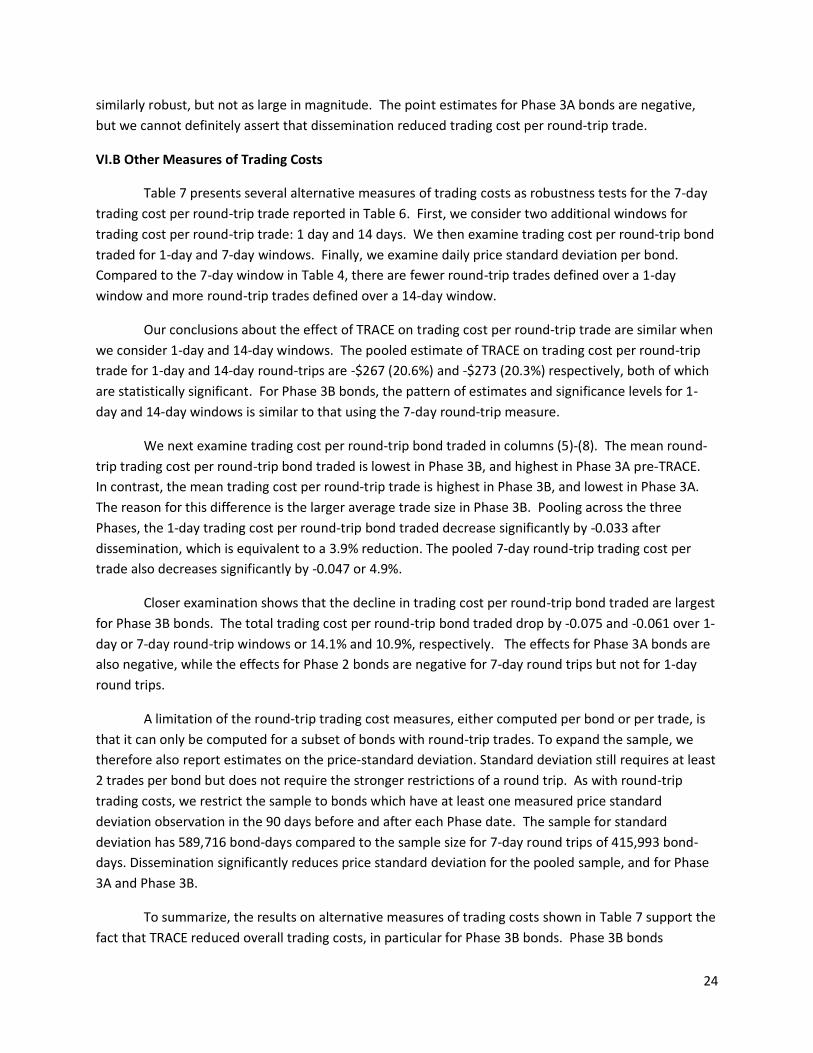
24

similarly robust, but not as large in magnitude. The point estimates for Phase 3A bonds are negative,

but we cannot definitely assert that dissemination reduced trading cost per round-trip trade.

VI.B Other Measures of Trading Costs

Table 7 presents several alternative measures of trading costs as robustness tests for the 7-day

trading cost per round-trip trade reported in Table 6. First, we consider two additional windows for

trading cost per round-trip trade: 1 day and 14 days. We then examine trading cost per round-trip bond

traded for 1-day and 7-day windows. Finally, we examine daily price standard deviation per bond.

Compared to the 7-day window in Table 4, there are fewer round-trip trades defined over a 1-day

window and more round-trip trades defined over a 14-day window.

Our conclusions about the effect of TRACE on trading cost per round-trip trade are similar when

we consider 1-day and 14-day windows. The pooled estimate of TRACE on trading cost per round-trip

trade for 1-day and 14-day round-trips are -$267 (20.6%) and -$273 (20.3%) respectively, both of which

are statistically significant. For Phase 3B bonds, the pattern of estimates and significance levels for 1-

day and 14-day windows is similar to that using the 7-day round-trip measure.

We next examine trading cost per round-trip bond traded in columns (5)-(8). The mean round-

trip trading cost per round-trip bond traded is lowest in Phase 3B, and highest in Phase 3A pre-TRACE.

In contrast, the mean trading cost per round-trip trade is highest in Phase 3B, and lowest in Phase 3A.

The reason for this difference is the larger average trade size in Phase 3B. Pooling across the three

Phases, the 1-day trading cost per round-trip bond traded decrease significantly by -0.033 after

dissemination, which is equivalent to a 3.9% reduction. The pooled 7-day round-trip trading cost per

trade also decreases significantly by -0.047 or 4.9%.

Closer examination shows that the decline in trading cost per round-trip bond traded are largest

for Phase 3B bonds. The total trading cost per round-trip bond traded drop by -0.075 and -0.061 over 1-

day or 7-day round-trip windows or 14.1% and 10.9%, respectively. The effects for Phase 3A bonds are

also negative, while the effects for Phase 2 bonds are negative for 7-day round trips but not for 1-day

round trips.

A limitation of the round-trip trading cost measures, either computed per bond or per trade, is

that it can only be computed for a subset of bonds with round-trip trades. To expand the sample, we

therefore also report estimates on the price-standard deviation. Standard deviation still requires at least

2 trades per bond but does not require the stronger restrictions of a round trip. As with round-trip

trading costs, we restrict the sample to bonds which have at least one measured price standard

deviation observation in the 90 days before and after each Phase date. The sample for standard

deviation has 589,716 bond-days compared to the sample size for 7-day round trips of 415,993 bond-

days. Dissemination significantly reduces price standard deviation for the pooled sample, and for Phase

3A and Phase 3B.

To summarize, the results on alternative measures of trading costs shown in Table 7 support the

fact that TRACE reduced overall trading costs, in particular for Phase 3B bonds. Phase 3B bonds

25

experience a significant and large reduction in round-trip trading cost per bond and per trade. The

percentage decrease in trading costs is between 10.9% and 29.0% depending on the measure.

VII. Additional Results

VII.A Trading Activity and Trading Costs by Trade Size

The difference between trading cost per round-trip trade and trading cost per round-trip bond

traded suggests that trade size must be considered in measuring the effects of dissemination. Moreover,

Table 4 suggested that Phase 3B bonds are more likely to trade in larger quantities because TRACE

regulations allow for some large Phase 3B trades to be disseminated with delay. Finally, a major

motivation for TRACE was to encourage participation by retail investors, who transact in smaller

quantities. For all these reasons, we next consider how trading activity and costs differ by trade size.

Table 8 reports 90-day difference-in-differences estimates on trading activity and costs pooled

and by Phases for three categories of trade sizes: < $100K (small), $100-$1M (medium), and $1M+

(large). We chose these categories because trades under $100K are often associated with retail trades,

and as discussed above, TRACE had dissemination provisions specific to trades greater than $1M+.

Panel A of Table 8 shows that roughly two-thirds of all trades are small. In the 90 days before

dissemination, 67.7% of all trades are small, and in the 90 days after dissemination, 68.9% are. In

contrast, most of the volume is accounted for by large trades, with 89.8% and 89.6% before and after

dissemination, respectively.

Panel B shows the effect of dissemination on the number of trades is significantly negative for

all three trade size categories, when pooled across Phases. The estimates range from -0.066 to -0.012,

or -12.2% to -8.6% for the three size categories. Although not shown in the Table, aggregating this

result across the size categories results in a decrease in the total number of trades of -0.096 which is

similar to the pooled effect on the number of trades reported in Table 4 of -0.088.

When split by Phase in Panel C, TRACE appears to have reduced the number of trades

differentially across Phases. Large trades drop significantly for Phase 2, medium-size trades drop for

Phase 2 and 3A, and small trades drop for Phase 3B. TRACE did not increase the number of trades for

any size and Phase combination.

The largest reduction in trading activity occurs for small trades in Phase 3B. In fact, almost the

entire reduction in the number of trades for Phase 3B is due to fewer small trades. Returning to the

question of the effect of the delayed dissemination provision for Phase 3B trades, we find that there is

not an increase in the number of large Phase 3B trades, even though there is an increase in average

trade size. The reason average trade size in Phase 3B increases is because small trades are taking place

less frequently, raising the average trade size. Thus, traders did not appear to increase their number of

large trades to avoid immediate dissemination.

Finally, these results in Table 9 mean that TRACE did not increase the number of small (retail)

trades as anticipated for any of the Phases, and significantly decreased it for Phase 3B.

26

Turning now to trading costs, the 7-day trading cost per round-trip trade for the three different

size categories are shown in columns (7) through (12). The 7-day trading cost per round-trip trade is

$209 for small trades and $6,276 for large trades. Pooling across Phases, TRACE reduced trading costs

significantly.

When split by Phase, trading costs decrease for each size and Phase combination, but not all are

significant. Trading costs decrease significantly for all size trades in Phase 3B. The largest reduction in 7-

day trading cost per round-trip trade is for medium size trades in Phase 3B, where the reduction is

26.9%.

VII.B Round-Trip Trading Costs by Trading Partner

Our analysis so far has not distinguished trades by customers from those by dealers. Customers

and dealers may trade for different reasons. Customers typically trade bonds for portfolio and life-cycle

reasons. Dealers may trade bonds for portfolio reasons, but also to intermediate between customers,

e.g., make a market. The effects of transparency on customers and dealers may also differ. For

example, the dissemination of transaction information may provide more new information to customers

than to dealers both because dealers typically transact more frequently and because active traders will

see many trade inquiries that are ultimately executed by other dealers. In this section, we will

investigate the effects of dissemination on Customer (C) and Dealer (D) trades separately.

The TRACE database only reports trades where one of the two parties is a dealer. These trades

can be between two dealers or between a customer and a dealer.31 Although not reported in a table,

Dealer-to-Dealer trades represents 28% of all trades and 24% of total volume. Trades in which a

customer sell to a dealer, Customer-to-Dealer, represent 31% of all trades (37% of total volume) and

trades in which a dealer sells to a customer, Dealer-to-Customer, trades are 40% of trades (39% of

volume).

Table 9 reports on round-trip trades, which we use to measure trading costs based on the

counterparties. In particular, a round trip can be one of three types: (1) Customer-Dealer-Customer

(CDC), (2) Dealer-Dealer-Dealer (DDD), and (3) Customer-Dealer-Dealer (CDD) or Dealer-Dealer-

Customer (DDC). The first two types of round-trip trade involve intermediation by a dealer since a

dealer need not hold inventory outside the round-trip time window. The other two categories imply

that a dealer is bearing risk outside the round-trip time window because some securities are held by

that dealer in inventory either before or after the trade.

Panel A of Table 9 shows that CDC trades represent roughly 25% of all round-trip trades, DDD

trades represent about 16% of all round-trip trades, and CDD/DDC trades are 59% of all round-trip

trades. We will use CDC trades as a proxy for customer trading costs and DDD trades as a proxy for

dealer trading costs.

31 FINRA members must report all trades in which they are involved. Trades between two parties, who are not FINRA members, are possible, but not recorded.

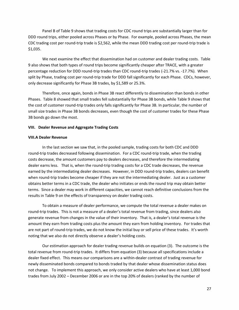
27

Panel B of Table 9 shows that trading costs for CDC round trips are substantially larger than for

DDD round trips, either pooled across Phases or by Phase. For example, pooled across Phases, the mean

CDC trading cost per round-trip trade is $2,562, while the mean DDD trading cost per round-trip trade is

$1,035.

We next examine the effect that dissemination had on customer and dealer trading costs. Table

9 also shows that both types of round trips become significantly cheaper after TRACE, with a greater

percentage reduction for DDD round-trip trades than CDC round-trip trades (-21.7% vs. -17.7%). When

split by Phase, trading cost per round-trip trade for DDD fall significantly for each Phase. CDCs, however,

only decrease significantly for Phase 3B trades, by $1,589 or 25.3%.

Therefore, once again, bonds in Phase 3B react differently to dissemination than bonds in other

Phases. Table 8 showed that small trades fell substantially for Phase 3B bonds, while Table 9 shows that

the cost of customer round-trip trades only falls significantly for Phase 3B. In particular, the number of

small size trades in Phase 3B bonds decreases, even though the cost of customer trades for these Phase

3B bonds go down the most.

VIII. Dealer Revenue and Aggregate Trading Costs

VIII.A Dealer Revenue

In the last section we saw that, in the pooled sample, trading costs for both CDC and DDD

round-trip trades decreased following dissemination. For a CDC round-trip trade, when the trading

costs decrease, the amount customers pay to dealers decreases, and therefore the intermediating

dealer earns less. That is, when the round-trip trading costs for a CDC trade decreases, the revenue

earned by the intermediating dealer decreases. However, in DDD round-trip trades, dealers can benefit

when round-trip trades become cheaper if they are not the intermediating dealer. Just as a customer

obtains better terms in a CDC trade, the dealer who initiates or ends the round trip may obtain better

terms. Since a dealer may work in different capacities, we cannot reach definitive conclusions from the

results in Table 9 on the effects of transparency on dealer trading costs.

To obtain a measure of dealer performance, we compute the total revenue a dealer makes on

round-trip trades. This is not a measure of a dealer’s total revenue from trading, since dealers also

generate revenue from changes in the value of their inventory. That is, a dealer’s total revenue is the

amount they earn from trading costs plus the amount they earn from holding inventory. For trades that

are not part of round-trip trades, we do not know the initial buy or sell price of these trades. It’s worth

noting that we also do not directly observe a dealer’s holding costs.

Our estimation approach for dealer trading revenue builds on equation (3). The outcome is the

total revenue from round-trip trades. It differs from equation (3) because all specifications include a

dealer fixed effect. This means our comparisons are a within-dealer contrast of trading revenue for

newly disseminated bonds compared to bonds traded by that dealer whose dissemination status does

not change. To implement this approach, we only consider active dealers who have at least 1,000 bond

trades from July 2002 – December 2006 or are in the top 20% of dealers (ranked by the number of

28

trades) in a Phase. A dealer that trades at least 1000 times or is in the top 20% for one Phase is included

as a dealer in all other Phases if they trade at least once in the other phases.32

Table 10 shows that, on average, across the three Phases a dealer’s revenue for round-trip

trades is $1,749. As with round-trip trading costs, the round-trip revenue is greatest in Phase 3B at

$3,789. This is partly a consequence of the fact that the average trade size is largest for Phase 3B bonds.

When comparing revenue per round-trip per bond traded, the revenue per bond traded is largest for

Phase 3A.

Dissemination causes a statistically significant reduction in dealer revenue per round-trip trade

pooled across Phases. This effect is driven by a large, statistically significant $1,246 reduction for Phase

3B bonds. This is equivalent to a 32.9% reduction in dealer trading revenue per trade. When measured

by revenue per round-trip bond traded, dealers also have a significant decrease of -0.845, or 12.7%, for

Phase 3B. None of the results for either round-trip per trade or round-trip per bond traded are

significant for Phase 2 or Phase 3A.

The large and significant effect on dealer revenue in Phase 3B with no effects in Phase 2 and 3A

are not surprising, given that dealer revenue on round-trip trades is closely related to round-trip trading

costs.

VIII.B Aggregate Economic Effects of TRACE

How economically large are the effects of TRACE estimated above? We have seen that TRACE

reduces the number of trades, particularly for Phase 3B bonds, but does not have a significant effect on

overall trading volume. TRACE also has a large and significant effect on trading costs and dealer

revenues. We next investigate the aggregate effects of TRACE by focusing on its effects on overall

trading costs and dealer revenues.

We benchmark our estimates against the overall level of transaction costs and revenues in the

corporate bond market. For this exercise, it is necessary to extrapolate our estimates of dissemination

effects along three dimensions. First, our research design does not allow us to construct an estimate of

the effect on bonds in Phase 1 or bonds that are not in any Phase. In particular, our research design

does not allow us to conclude much about the first Phase of TRACE.33 Second, our research design

32 Most members of FINRA are not active corporate bond dealers. There are 2,639 unique hashcodes for dealers from July 2002 – December 2006 in our data. The mean number of trades for a dealer is 7,751 and the median is 74. Using our definition above, we are left with 599 unique dealers that trade 98.6% of all trades and 99.4% of all volume in our data. 33 Using a sample of NAIC bonds, Bessembinder, Maxwell, and Venkataraman (2006) argue TRACE reduced transaction costs [they use the term trade execution costs] for Phase 1 bonds. It is possible to measure bond trading activity for NAIC bonds before Phase 1 of TRACE. In Appendix A, we use data from the NAIC together with our difference-in-differences methodology to examine Phase 1 effects. Unlike our TRACE sample, we are not able to construct a round-trip cost estimate. The Appendix shows two main facts. First, NAIC bond trading has different characteristics than TRACE trading. NAIC bonds are larger and transact less frequently. They also contain very few Phase 3B bonds. Second, using our research design, there is no evidence that TRACE influenced NAIC trading activity or costs for Phase 1 bonds.

29

focuses on the 180 days surrounding dissemination, while our sample period covers 4.5 years from July

2002 through December 2006. Finally, since round-trip trades only represent about 35% of all trading

activity, we need to apply our estimate to the remaining trades that are not part of round-trip trades.

Panel A of Table 11 first uses our estimate of pooled trading cost per round-trip trade as the

basis for extrapolation. If we assume that the mean round trip in the 90 days prior to dissemination

pooled across Phases represents the average trading cost per round-trip trade for the 22.6 million trades

during our time period, the total costs of trading bonds is $14.7 billion. Pooled across Phases, TRACE

reduced the average trading cost per round-trip trade by -$241, which would amount to a $2.7 billion

reduction in trading costs. Since our time period covers 4.5 years, this translates to a reduction in

trading costs of $605 million per year.

We have also seen that TRACE has different effects across Phases. A second estimate of the

reduction in trading costs takes the average trade cost and dissemination estimates by Phase and

applies it to trading activity specific to each Phase. To implement this approach, we still need to ascribe

a value of trading costs and the effect of TRACE to bonds in Phase 1 and bonds that do not have a Phase.

Table 11 reports aggregate estimates broken down by Phase which use values from Phase 2 for Phase 1,

and the pooled estimate for bonds that are not in a Phase. The total reduction in trading costs per year

from this more refined comparison is $538 million per year. Importantly, trading in Phase 3B bonds

contributes to a 21.8% share of this aggregate reduction, even though Phase 3B only accounts for 5.1%

of all trades. This fact further highlights that studies of TRACE without Phase 3B bonds miss a large part

of the aggregate picture.

Table 11 also aggregates the reduction in dealer revenue from round-trip trades, using the

estimate from Table 10. The results for this outcome are shown in Panel B. When the pooled estimate

is applied to all trades, we find a $695 million per year reduction in dealer revenue due to TRACE. When

split by Phase in the same way as in Panel A, the estimated reduction in dealer revenue per year is $460

million. The reason the estimate is smaller by Phase is that when split by Phase, a large decrease in

dealer revenue only appears for Phase 3B. As with trading costs, Phase 3B stands out as contributing an

outsize share of the reduction in dealer revenue of 34.5% compared to the number of trades in Phase 3B

bonds.

Since our estimates show little overall effect on trading volume, the reduction in dealer

revenues is largely a transfer from dealers to customers. That is, customers pay less to transact at the

expense of dealers but experience no overall reduction in trading activity as measured by volume.

It’s worth emphasizing that the interpretation of the effect on trading activity is not

straightforward absent a view on why corporate bonds trade. First, we find a decrease in the number

of trades. This might influence how quickly prices reflect new information. Moreover, trading activity

outcomes are a consequence of the demand and supply for trades: they do not directly speak to

whether trading has become more difficult, say if dealers are less willing to hold inventory because of

the cut in their margins.

30

VIII. Conclusion

The introduction of TRACE, which was implemented in four Phases over a three-and-a-half-year

period, combined with the availability trading records before and after dissemination for three of the

Phases, provides a unique opportunity to study how previously opaque over-the-counter financial

markets respond to transparency. We use a difference-in-differences research design to isolate the

effect of post-trade transparency from underlying market trends, holding fixed all other institutional

aspects of corporate bond trading. Our study is distinguished by the fact that we examine all Phases of

TRACE, including the less frequently-traded bonds in the last two Phases of TRACE, which have small

issue sizes and low-credit quality, respectively. It also directly measures round-trip trading costs for all

bonds across all four Phases.

Our main finding is that TRACE causes trading costs to decline significantly for the entire bond

market and for both dealers and customers. In addition, we find the impact on trading activity and

trading costs are largest and most significant for Phase 3B bonds. After transparency, there is a

significant decline in the number of trades for Phase 3B bonds, and a large significant reduction in

trading costs. These results stand out because at the time of Phase 3B, TRACE’s dissemination

provisions had already been implemented for three previous Phases covering a majority of bonds issued.

Bonds in Phase 3B also play an outsized role in our estimates of the aggregate effect of transparency on

total trading costs. Thus, studies of TRACE and transparency that do not examine this segment of the

market are incomplete.

The results also confirm that transparency has a limited impact on trading activity of investment

grade bonds and the most frequently-traded bonds. There is no significant decrease in trading activity,

either measured by number of trades or trading volume for this segment of the market. On the other

hand, TRACE does not increase overall trading activity, as many proponents anticipated. This is

noteworthy given the significant reduction in trading costs.

These findings have several other implications. The sharp pervasive reduction in trading costs

may be a consequence of the fact that trading information changes the relative bargaining positions of

investors and dealers, allowing investors to benefit at the expense of dealers. Our best estimate is that

TRACE transferred about $600 million a year from dealers to customers. Since transparency has negative

effects for some trading partners, our result may suggest why transparency reforms need to be

mandated rather than voluntarily adopted.

These results are also relevant for current and planned expansions of mandated market

transparency. The implicit assumption underlying the use of TRACE as a template for regulations such

as Dodd-Frank is that transparency affects all segments of a market the same way. Our results show

that transparency effects are not uniform across different segments of the bond market. Many of the

securities markets that are newly subject to transparency are akin to Phase 3B bonds. That is, they are

infrequently traded and may not be widely held across dealers. As a consequence, our results support

the view that not every segment of a security market should be subject to the same degree of mandated

transparency.

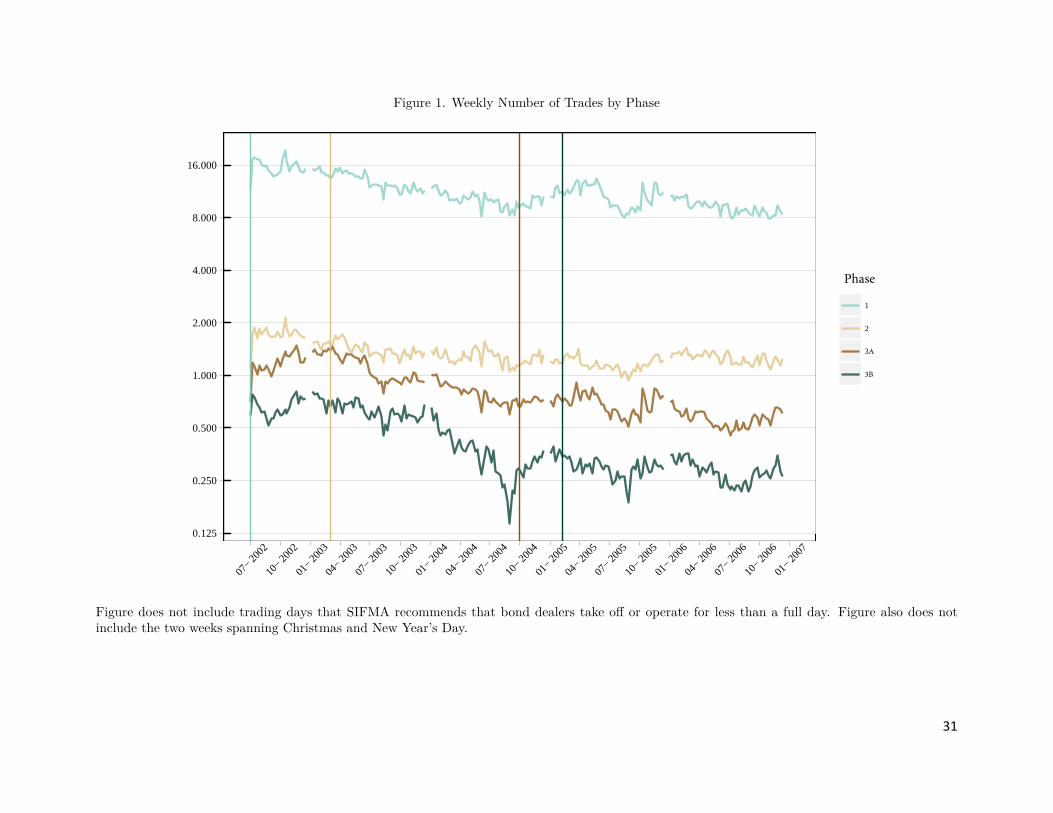
Figure 1. Weekly Number of Trades by Phase

0.125

0.250

0.500

1.000

2.000

4.000

8.000

16.000

07−20

0210

−2002

01−20

0304

−2003

07−20

0310

−2003

01−20

0404

−2004

07−20

0410

−2004

01−20

0504

−2005

07−20

0510

−2005

01−20

0604

−2006

07−20

0610

−2006

01−20

07

1

2

3A

3B

Figure does not include trading days that SIFMA recommends that bond dealers take off or operate for less than a full day. Figure also does notinclude the two weeks spanning Christmas and New Year’s Day.

Phase

31

Figure 2. Weekly 7-Day Trading Cost per Round-trip Trade by Phase

0

2500

5000

7500

07−20

0210

−2002

01−20

0304

−2003

07−20

0310

−2003

01−20

0404

−2004

07−20

0410

−2004

01−20

0504

−2005

07−20

0510

−2005

01−20

0604

−2006

07−20

0610

−2006

01−20

07

1

2

3A

3B

Figure does not include trading days that SIFMA recommends that bond dealers take off or operate for less than a full day. Figure also does notinclude the two weeks spanning Christmas and New Year’s Day.

2

Phase

32

Figure 3. Event Study for Number of Trades

−0.3

0.0

0.3

−10 −5 0 5 10week

Phase 2

−0.50

−0.25

0.00

0.25

0.50

−10 −5 0 5 10week

Phase 3A

−0.8

−0.4

0.0

0.4

0.8

−10 −5 0 5 10week

Phase 3B

Figure plots coefficients on Disseminate x Week variables from event study regressions where the dependentvariable is weekly number of trades. Disseminate is an indicator for a bond that becomes disseminated inthe Phase. The x-axes represent weeks, where, 0 is week of March 3, 2003 for Phase 2, 0 is week of October1, 2004 for Phase 3A, and 0 is week of February 7, 2005 for Phase 3B.

33

Figure 4. Event Study for 7-Day Trading Cost per Round-trip Trade by Phase

−800

−400

0

400

800

−10 −5 0 5 10week

Phase 2

−800

−400

0

400

800

−10 −5 0 5 10week

Phase 3A

−2000

0

2000

−10 −5 0 5 10week

Phase 3B

Figure plots coefficients on Disseminate x Week variables from event study regressions where the dependentvariable is weekly trading cost per round-trip trade. Disseminate is an indicator for a bond that becomesdisseminated in the Phase. The x-axes represent weeks, where, 0 is week of March 3, 2003 for Phase 2, 0 isweek of October 1, 2004 for Phase 3A, and 0 is week of February 7, 2005 for Phase 3B.

34

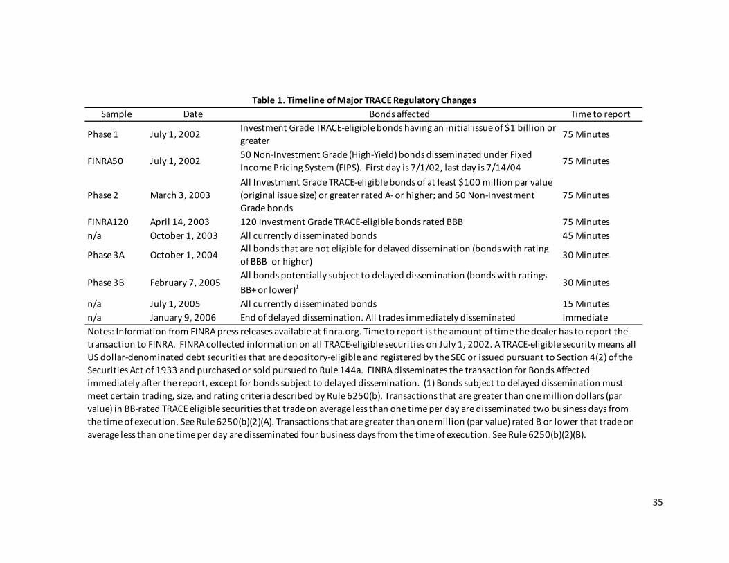
Sample Date Bonds affected Time to report

Phase 1 July 1, 2002Investment Grade TRACE-eligible bonds having an initial issue of $1 billion or greater

75 Minutes

FINRA50 July 1, 200250 Non-Investment Grade (High-Yield) bonds disseminated under Fixed Income Pricing System (FIPS). First day is 7/1/02, last day is 7/14/04

75 Minutes

Phase 2 March 3, 2003All Investment Grade TRACE-eligible bonds of at least $100 million par value (original issue size) or greater rated A- or higher; and 50 Non-Investment Grade bonds

75 Minutes

FINRA120 April 14, 2003 120 Investment Grade TRACE-eligible bonds rated BBB 75 Minutesn/a October 1, 2003 All currently disseminated bonds 45 Minutes

Phase 3A October 1, 2004All bonds that are not eligible for delayed dissemination (bonds with rating of BBB- or higher)

30 Minutes

Phase 3B February 7, 2005All bonds potentially subject to delayed dissemination (bonds with ratings BB+ or lower)1 30 Minutes

n/a July 1, 2005 All currently disseminated bonds 15 Minutesn/a January 9, 2006 End of delayed dissemination. All trades immediately disseminated Immediate

Table 1. Timeline of Major TRACE Regulatory Changes

Notes: Information from FINRA press releases available at finra.org. Time to report is the amount of time the dealer has to report the transaction to FINRA. FINRA collected information on all TRACE-eligible securities on July 1, 2002. A TRACE-eligible security means all US dollar-denominated debt securities that are depository-eligible and registered by the SEC or issued pursuant to Section 4(2) of the Securities Act of 1933 and purchased or sold pursued to Rule 144a. FINRA disseminates the transaction for Bonds Affected immediately after the report, except for bonds subject to delayed dissemination. (1) Bonds subject to delayed dissemination must meet certain trading, size, and rating criteria described by Rule 6250(b). Transactions that are greater than one million dollars (par value) in BB-rated TRACE eligible securities that trade on average less than one time per day are disseminated two business days from the time of execution. See Rule 6250(b)(2)(A). Transactions that are greater than one million (par value) rated B or lower that trade on average less than one time per day are disseminated four business days from the time of execution. See Rule 6250(b)(2)(B).

35

Phase 1 Phase 2 Phase 3A Phase 3B(1) (2) (3) (4)

Number of bonds 388 2,526 11,081 2,859

Size at issue ($M) mean 1,463 264 86 184 p5 750 100 1 2 p10 1,000 100 1 8 p25 1,000 150 3 87 median 1,250 200 12 150 p75 1,750 300 80 238 p90 2,500 500 300 350 p95 3,000 600 425 470

Rating at phase start mean A A+ A- B p5 AAA AAA AAA BBB- p10 AA- AA AA BB+ p25 A+ A+ A BB- median A A+ A- B p75 BBB+ A BBB CCC p90 BBB A- BBB- D p95 BBB- A- BB+ D# with rating information at phase start 388 2,524 11,046 2,770# where rating is from S&P RatingsXpress 366 2,182 7,754 2,283# where rating is from FISD 22 342 3,292 487

Fixed coupon rate mean 6.7 6.9 5.8 9.0 median 6.8 6.9 5.9 8.8 number fixed coupon 346 2,149 10,153 2,638

Maturity at issue (years) mean 9.2 15.0 11.8 12.4 median 6.0 10.0 10.0 9.7

Years since issue (at phase start) mean 1.9 5.5 3.3 5.9 median 1.4 5.1 1.9 5.7

Table 2. Bond Characteristics by Phase

Notes: Bond issue size, coupon, maturity, and issue date characteristics are from FISD. Bond rating are the most recent rating before the Phase starts. Bond rating characteristics are from S&P RatingsXPress database. If ratings are not available in S&P RatingsXpress, we use ratings from FISD. To assign a FISD rating, we first use the S&P value if it exists, otherwise the Moody’s value, otherwise the Fitch value, and otherwise the Duff and Phelps value. Mean ratings are computed by first converting each rating to a number (AAA=1, AA+=2, AA=3, …, and D=22) and then converting the number back to a letter rating.

36

90 days before 90 days after 90 days before 90 days after(1) (2) (3) (4)

Phase 1 (N=388) - 15.527 Phase 1 (N=381) - 1,682Phase 2 (N=2,526) 1.502 1.538 Phase 2 (N=1,967) 1,413 1,053Phase 3A (N=11,081) 0.696 0.691 Phase 3A (N=6,151) 947 822Phase 3B (N=2,859) 0.332 0.315 Phase 3B (N=1,106) 4,030 2,920

Phase 1 (N=388) - 12,440,080 Phase 1 (N=381) - 0.568Phase 2 (N=2,526) 952,667 876,079 Phase 2 (N=1,967) 0.806 0.790Phase 3A (N=11,081) 377,875 354,424 Phase 3A (N=6,151) 1.087 1.007Phase 3B (N=2,859) 387,815 376,500 Phase 3B (N=1,106) 0.561 0.434

Phase 1 (N=388) … 0.902 Phase 1 (N=388) … 0.988Phase 2 (N=2,526) 0.297 0.273 Phase 2 (N=2,042) 0.875 0.861Phase 3A (N=11,081) 0.163 0.164 Phase 3A (N=6,369) 0.862 0.806Phase 3B (N=2,859) 0.187 0.169 Phase 3B (N=1,206) 0.554 0.480

Table 3. Trading Activity and Trading Cost around Phase Start

Notes: Sample for number of trades is restricted to bonds in either the 90 calendar days before or after the Phase start. If a bond does not trade, it contributes to zero trades for that day. The mean reported above is the average daily number of trades in the 90-day window. The sample for average daily volume is constructed like that of trades and the daily volume is averaged over all bond-days in the 90-day window. Average daily volume/issue size is the average of daily volume/issue size calculated in the same manner as average daily volume. For round-trip trading cost measures, we measure the price difference between the two trades in a chain that span at most 7 calendar days (including the day of the first trade). The sample of bonds is restricted to bonds where there is at least one day in the 90 days before the Phase start with at least one chain and at least one chain after. The trading cost per round-trip bond traded is the difference in price per bond between the second and the first trade in the chain (in $100 par). The trading cost per round-trip trade is the difference in price per bond times the number of bonds. The reported average for the round-trip measures is average of bond-day mean over all bond-days in the 90-day window. The sample for daily price standard deviation is constructed as the round-trip measures but with the additional requirement of having at least two trades both before and after the start of the Phase. After computing the within-day price standard deviation for each bond for all days with at least two trades, we average across these days during either the 90 days before or after the Phase start. Price standard deviation is the average daily price standard deviation across these bonds. There is no transaction information for Phase 1 bonds in the 90 days before Phase 1 starts. N refers to the number of bonds in the sample that change dissemination status in the Phase.

Number of trades per bond-day

Volume per day ($)

7-day trading cost per round-trip trade ($)

7-day trading cost per round-trip bondtraded ($)

Price standard deviation ($)Volume/Issue size per day

Trading costTrading activity

37

90-day mean for

disseminated before phase

start

60 days 90 days 180 days

With linear and quadratic trends specific to investment grade for each

Phase

Without Phase 1 bonds

as controls

Sample matched on size, time to

maturity, and years since

issuance

(1) (2) (3) (4) (5) (6) (7)

All three phases 0.754 -0.069*** -0.088*** -0.092*** -0.033 -0.030 -0.094***(0.027) (0.026) (0.028) (0.026) (0.021) (0.033)-9.1% -11.7% -12.2% -4.4% -4.0% -12.5%

Phase 2 1.502 0.094** -0.033 -0.093** 0.005 -0.069* -0.054(0.047) (0.041) (0.041) (0.045) (0.038) (0.059)

6.3% -2.2% -6.2% 0.3% -4.6% -3.6%

Phase 3A 0.696 -0.132*** -0.048 -0.041 -0.029 -0.004 -0.109**(0.044) (0.038) (0.045) (0.037) (0.036) (0.055)-19.0% -6.9% -5.9% -4.2% -0.6% -15.7%

Phase 3B 0.332 -0.238*** -0.236*** -0.169*** -0.194*** -0.001 -0.140***(0.042) (0.062) (0.065) (0.034) (0.022) (0.046)-71.7% -71.1% -50.9% -58.4% -0.3% -42.2%

0.000 0.017 0.269 0.000 0.000 0.000

# of Phase 2 bonds 2,526 2,526 2,526 2,524 2,526 2,524# of Phase 3A bonds 11,081 11,081 11,081 11,044 11,081 4,421# of Phase 3B bonds 2,859 2,859 2,859 2,768 2,859 2,859

# of trades for Phase 2 1,496,633 2,116,395 4,132,239 2,105,872 1,503,471 2,046,291# of trades for Phase 3A 1,022,128 1,530,186 3,174,160 1,525,675 1,189,969 1,390,655# of trades for Phase 3B 506,245 753,767 1,446,740 750,593 372,431 753,767

# of bond-days 2,320,998 3,421,074 6,804,827 3,386,963 3,310,621 2,317,302Notes: This table reports estimates of Disseminate x Post for number of trades. Panel A reports estimates from Phases 2, 3A, and 3B pooled together, while panel B reports estimates for each Phase separately. Robust standard errors clustered by bond and Phase are in parenthesis immediately below the estimates. All models include bond fixed effects. Mean for Disseminated is the 90-day average for newly disseminated bonds immediately before the Phase start. The third entry in each row is the percentage effect as computed by dividing the estimate by the Mean for Disseminated. Phase effects equal reports p-values of tests that the three Phase estimates are equal. The 60-day regressions use trades from 60 calendar days before and after the Phase change. The 90- and 180-day regressions are defined analogously. There are 8,324 Phase 2, 2,235 Phase 3A, and 2,129 Phase 3B control bonds in columns (2)-(4). Standard errors in parentheses. The model with trends in column (5) has linear and quadratic functions of time for investment grade and high-yield bonds specific to each Phase. Column (6) excludes Phase 1 bonds as controls for Phase 2, 3A and 3B. The characteristics used to construct the matched sample in column (7) are issue size at Phase start, time to maturity at Phase start, and years since issue at Phase start. We divide the sample into four issue size quartiles, and two groups for the other two characteristics: above/below the median time to maturity and years since issue. We exclude bonds in cells with 5 or fewer treated bonds or 5 or fewer control bonds. * significant at 10%; ** significant at 5%; *** significant at 1%

A. Pooled

B. By phase

Alternative specifications (90-day window)Table 4. Difference-in-Difference Estimates for Number of Trades

H0: Phase effects equal (p-val)

Alternative time windows

38

Mean Estimate Mean Estimate Mean Estimate(1) (2) (3) (4) (5) (6)

All three phases 462,897 -25,177 0.186 -0.012** 649,910 3,189(20,264) (0.005) (10,702)

-5.4% -6.5% 0.5%

Phase 2 952,667 -66,553** 0.297 -0.039*** 709,546 -9,121(32,934) (0.009) (18,210)

-7.0% -13.1% -1.3%

Phase 3A 377,875 -34,729 0.163 0.007 541,930 -968(34,815) (0.007) (14,768)

-9.2% 4.3% -0.2%

Phase 3B 387,815 55,890 0.187 0.003 1,178,134 50,101**(37,133) (0.008) (25,197)

14.4% 1.6% 4.3%

H0: Phase effects equal (p-val) 0.042 0.000 0.138

# of trades 4,533,784 4,579,932 4,556,139# of bond-days 3,421,206 3,421,431 864,168

Table 5. Estimates for Alternate Measures of Trading Activity (90-day Window)

Notes. This table reports estimates of Disseminate x Post for alternative measures of trading activity following the 90-day estimates in column (3) of Table 4. The Average Trade Size measure requires that there be at least one trade for a bond in the before and the after period to be included in the sample. See Table 4 notes for additional details.* significant at 10%; ** significant at 5%; *** significant at 1%

A. Pooled

B. By phase

Volume ($) Volume/Issue size Average trade size

39

90-day mean for

disseminated before phase

start

60 days 90 days 180 days

With linear and quadratic trends specific to investment grade for each

Phase

Without Phase 1 bonds

as controls

Sample matched on size, time to

maturity, and years since

issuance

(1) (2) (3) (4) (5) (6) (7)

All three phases 1,301 -230*** -241*** -192*** -141*** -244*** -228***(60) (51) (40) (49) (59) (65)

-17.7% -18.5% -14.8% -10.8% -18.8% -17.5%

Phase 2 1,413 -282*** -250*** -60 -205** -241** -230**(104) (87) (72) (86) (96) (106)

-20.0% -17.7% -4.2% -14.5% -17.1% -16.3%

Phase 3A 947 -19 -54 -73** -20 -13 -46(56) (46) (33) (44) (52) (65)

-2.0% -5.7% -7.7% -2.1% -1.4% -4.9%

Phase 3B 4,030 -813*** -924*** -1,224*** -694** -969*** -858***(234) (225) (164) (296) (222) (256)

-20.2% -22.9% -30.4% -17.2% -24.0% -21.3%

0.001 0.000 0.000 0.017 0.000 0.005

# of Phase 2 bonds 1,841 1,966 2,123 1,965 1,967 1,966# of Phase 3A bonds 5,225 6,151 7,623 6,140 6,150 2,787# of Phase 3B bonds 959 1,106 1,281 1,089 1,106 1,106

# of round-trips for Phase 2 295,540 413,813 808,282 411,830 283,895 399,824# of round-trips for Phase 3A 185,810 284,456 608,293 283,513 225,295 245,586# of round-trips for Phase 3B 96,152 145,334 275,367 144,710 71,848 145,340

# of bond-days 279,678 416,004 839,624 414,203 347,644 371,344Notes: This table reports estimates of Disseminate x Post for 7-day trading cost per round-trip trade. There are 8,324 Phase 2, 2,235 Phase 3A, and 2,129 Phase 3B control bonds in columns (2)-(4). See Table 4 notes for details. * significant at 10%; ** significant at 5%; *** significant at 1%

A. Pooled

Table 6. Estimates for 7-Day Trading Cost per Round-trip TradeAlternative specifications (90-day window)

H0: Phase effects equal (p-val)

B. By phase

Alternative time windows

40

Mean Estimate Mean Estimate Mean Estimate Mean Estimate Mean Estimate(1) (2) (3) (4) (5) (6) (7) (8) (9) (10)

All three phases 1,299 -267*** 1,344 -273*** 0.842 -0.033*** 0.964 -0.047*** 0.841 -0.021***(46) (58) (0.006) (0.007) (0.005)

-20.6% -20.3% -3.9% -4.9% -2.5%

Phase 2 1,318 -131 1,448 -387*** 0.666 0.008 0.806 -0.027** 0.875 -0.003(84) (99) (0.010) (0.011) (0.009)

-9.9% -26.7% 1.2% -3.3% -0.3%

Phase 3A 965 -164*** 996 52 0.970 -0.064*** 1.087 -0.065*** 0.862 -0.033***(36) (59) (0.009) (0.010) (0.007)

-17.0% 5.2% -6.6% -6.0% -3.8%

Phase 3B 4,017 -1,166*** 4,070 -1,072*** 0.532 -0.075*** 0.561 -0.061*** 0.554 -0.042***(186) (237) (0.016) (0.018) (0.012)

-29.0% -26.3% -14.1% -10.9% -7.6%

H0: Phase effects equal (p-val) 0.000 0.000 0.000 0.000 0.011

# of round-trips/trades 715,950 891,664 715,978 843,609 4,271,416# of bond-days 365,946 430,484 365,954 415,993 589,716

B. By phase

Notes. This table reports estimates of Disseminate x Post for alternative measures of trading cost following the 90-day estimates in column (3) of Table 6. 1-day and 14-day round-trips are constructed similar to the 7-day round-trips with the restriction that the two trades in the round-trip span at most 1 and 14 calendar day (including the day of the first trade) respectively. Trading cost per round-trip bond traded is the difference in price per bond between the second and the first trade in the round-trip at $100 par. The trading cost per round-trip trade measures the total cost (difference in price per bond times the number of bonds). The daily price standard deviation is the within-day price standard deviation.

Table 7. Estimates for Alternative Measures of Trading Cost (90-day window)

1-day 14-dayTrading cost per round-trip bond tradedTrading cost per round-trip trade

1-day 7-day

A. Pooled

Daily price standard deviation (all trades)

41

(1) (2) (3) (4) (5) (6) (7) (8) (9) (10) (11) (12)

Before After Before After Before After Before After Before After Before After# of trades/round-trips 1,440,045 1,568,370 359,352 368,930 328,473 337,924 274,710 315,429 59,562 63,405 53,780 56,685Share of trades/round-trips 67.7% 68.9% 16.9% 16.2% 15.4% 14.9% 70.8% 72.4% 15.3% 14.6% 13.9% 13.0%

Volume ($M) 31,903 34,302 106,948 107,681 1,221,074 1,226,051 3,092 3,342 12,797 12,934 117,017 119,310Share of volume 2.3% 2.5% 7.9% 7.9% 89.8% 89.6% 2.3% 2.5% 9.6% 9.5% 88.0% 88.0%

Mean Estimate Mean Estimate Mean Estimate Mean Estimate Mean Estimate Mean Estimate

All three phases 0.539 -0.066*** 0.139 -0.012*** 0.204 -0.018*** 209 -8*** 950 -106*** 6,276 -1,031***(0.023) (0.004) (0.005) (2) (24) (322)-12.2% -8.6% -8.8% -3.8% -11.2% -16.4%

Phase 2 1.126 0.020 0.331 -0.019** 0.212 -0.029*** 187 -5 868 -82** 7,056 -1,191**(0.036) (0.008) (0.009) (3) (37) (603)

1.8% -5.7% -13.7% -2.7% -9.4% -16.9%

Phase 3A 0.514 -0.032 0.106 -0.013** 0.223 -0.011 218 -8*** 971 -59* 5,222 -498(0.031) (0.006) (0.009) (3) (35) (412)-6.2% -12.2% -4.9% -3.7% -6.1% -9.5%

Phase 3B 0.131 -0.251*** 0.098 0.001 0.148 -0.011 218 -31*** 1,215 -327*** 8,439 -1,664***(0.056) (0.010) (0.010) (11) (75) (615)

-191.8% 1.0% -7.4% -14.2% -26.9% -19.7%

H0: Phase effects equal (p-val) 0.000 0.274 0.294 0.081 0.005 0.258

# of trades/round-trips 3,008,415 728,282 666,397 590,139 122,967 110,465# of bond-days 3,190,387 2,341,085 309,770 309,770 90,667 74,087

A. Summary statistics

B. Pooled

C. By phase

Notes: This table reports estimates of Disseminate x Post for number of trades and 7-day trading cost per round-trip trade split by trade size. Numbers in Panel A exclude Phase 1. The specifications follow those for the 90-day estimate in column (3) of Tables 4 and 6. * significant at 10%; ** significant at 5%; *** significant at 1%

Table 8. Estimates by Trade SizeNumber of trades Trading cost per round-trip trade

Vol < $100k $100k <= Vol < $1Mil Vol >= $1Mil Vol < $100k $100k <= Vol < $1Mil Vol >= $1Mil

42

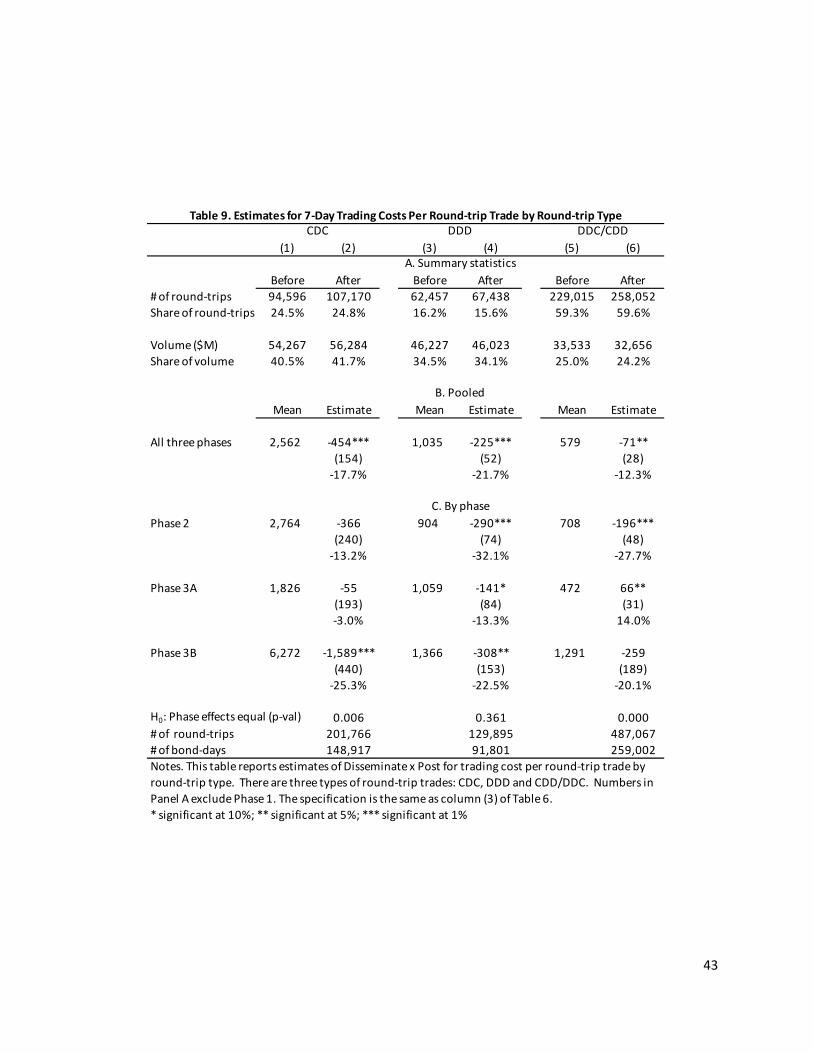
(1) (2) (3) (4) (5) (6)

Before After Before After Before After# of round-trips 94,596 107,170 62,457 67,438 229,015 258,052Share of round-trips 24.5% 24.8% 16.2% 15.6% 59.3% 59.6%

Volume ($M) 54,267 56,284 46,227 46,023 33,533 32,656Share of volume 40.5% 41.7% 34.5% 34.1% 25.0% 24.2%

Mean Estimate Mean Estimate Mean Estimate

All three phases 2,562 -454*** 1,035 -225*** 579 -71**(154) (52) (28)

-17.7% -21.7% -12.3%

Phase 2 2,764 -366 904 -290*** 708 -196***(240) (74) (48)

-13.2% -32.1% -27.7%

Phase 3A 1,826 -55 1,059 -141* 472 66**(193) (84) (31)-3.0% -13.3% 14.0%

Phase 3B 6,272 -1,589*** 1,366 -308** 1,291 -259(440) (153) (189)

-25.3% -22.5% -20.1%

0.006 0.361 0.000# of round-trips 201,766 129,895 487,067# of bond-days 148,917 91,801 259,002

C. By phase

Notes. This table reports estimates of Disseminate x Post for trading cost per round-trip trade by round-trip type. There are three types of round-trip trades: CDC, DDD and CDD/DDC. Numbers in Panel A exclude Phase 1. The specification is the same as column (3) of Table 6. * significant at 10%; ** significant at 5%; *** significant at 1%

Table 9. Estimates for 7-Day Trading Costs Per Round-trip Trade by Round-trip TypeCDC DDD DDC/CDD

A. Summary statistics

B. Pooled

H0: Phase effects equal (p-val)

43

Mean Estimate Mean Estimate(1) (2) (3) (4)

All three phases 1,749 -277*** 7.490 -0.0617(93) (0.0942)

-15.8% -0.8%

Phase 2 1,818 -146 5.442 0.115(145) (0.132)-8.0% 2.1%

Phase 3A 1,171 20 8.902 0.112(107) (0.155)1.7% 1.3%

Phase 3B 3,789 -1,246*** 6.645 -0.845***(289) (0.228)

-32.9% -12.7%

0.000 0.001# of round-trips 839,184 839,196# of dealer-days 152,190 152,187Notes. This table reports estimates of Disseminate x Post for dealer revenues from 7-day round-trips. We only include dealers that have at least 1,000 trades from July 2002 - December 2006 or are in the top 20% of the dealers (ranked by number of trades) trading in that phase. A dealer that meets the above criteria in a phase is also included in other phases conditional on them trading at least once in that phase. There are 590 dealers in Phase 2, 599 in Phase 3A, and 590 in Phase 3B. See Table 4 notes for details.* significant at 10%; ** significant at 5%; *** significant at 1%

Table 10. Daily Dealer Revenue in 7-day Round-tripsRevenue per round-

trip tradeRevenue per round-

trip bond traded

A. Pooled

B. By phase

H0: Phase effects equal (p-

44

Number of trades (Jul 02-Dec 06)

Mean per round-trip (90-day pre-period)

Total cost/revenue (Jul 02-Dec 06)

Reduction per round-trip (90-day pre-

period)

Total reduction in cost/revenue (Jul 02-

Dec 06)

Reduction in cost/revenue per

year(1) (2) (3) (4) (5) (6)

Phase+No phase 22,582,689 1,301 14,690,892,594 241 2,721,214,025 604,714,228

Phase 1 4,130,856 1,413 2,918,256,531 250 516,357,000 114,746,000Phase 2 2,934,629 1,413 2,073,178,112 250 366,828,625 81,517,472Phase 3A 7,742,494 947 3,665,481,341 54 209,047,338 46,454,964Phase 3B 1,144,757 4,030 2,306,807,581 924 528,877,734 117,528,385No Phase 6,629,953 1,301 4,313,034,972 241 798,909,337 177,535,408Total 22,582,689 15,276,758,537 2,420,020,034 537,782,230

Phase+No phase 22,582,689 1,749 19,743,034,532 277 3,127,702,427 695,044,984

Phase 1 4,130,856 1,818 3,754,031,000 146 301,552,488 67,011,664Phase 2 2,934,629 1,818 2,666,926,235 146 214,227,917 47,606,204Phase 3A 7,742,494 1,171 4,531,725,154 -20 -77,424,940 -17,205,542Phase 3B 1,144,757 3,789 2,168,533,063 1,246 713,183,611 158,485,247No Phase 6,629,953 1,749 5,796,271,251 277 918,248,491 204,055,220Total 22,582,689 18,917,486,705 2,069,787,567 459,952,793

Table 11. Aggregate Reduction in Trading Cost and Dealer Revenue

Panel A. Trading cost: cost per round-trip trade

Panel B. Dealer revenue: revenue per round-trip trade

This table estimates the aggregated reduction in trading cost and dealer revenue per year in the corporate bond market because of the transparency. Panel A measures the reduction in trading cost and Panel B measures the reduction in dealer revenue. In both the panels, Phase + No Phase uses the aggregate all phase estimates. For Phase 1, we use the estimates for Phase 2 (the means in table 2 for Phase 1 and 2 are similar) and for No Phase, we use the aggregate estimates. In Panel A, the estimates in column (2) and (4) for trading cost per round-trip trade measures are from Table 6. In Panel B, the estimates in column (2) and (4) for revenue per round-trip trade are from Table 10.

45

46

Appendix A: NAIC analysis and Phase 1

In this Appendix, we briefly review the National Association of Insurance Companies (NAIC)

database and use it to study Phase 1. Although TRACE data did not exist before July 2, 2002, the NAIC

maintains trading records for member insurance companies since 1994. Bessembinder, Maxwell, and

Venkataraman (2006) use NAIC transaction data to estimate trade execution costs in Phase 1 and other

Phases and argue that there are spillovers from Phase 1 to other Phases.

We use our methodology on the NAIC database to examine the effects of Phase 1 of TRACE.

There are two important differences between our approach and Bessembinder, et al. First, we use a

difference-in-differences research design. Second, we directly measure price standard deviation as a

proxy for trading costs, rather than using a structural model of trading to impute trading costs.

We find that TRACE does not have a significant effect on price standard deviation using NAIC

data. Further, our analysis of TRACE above shows significant negative effects on both trading costs and

price standard deviation due to dissemination for Phase 3B bonds. It is therefore a surprise that we do

not find similar results for Phase 1. If there are spillover effects from Phase 1, we would have expected

smaller, rather than larger, results for subsequent Phases.

While using the NAIC database, we discovered a systematic error in how NAIC’s trades are

reported. Many NAIC trades are disaggregated and reported as multiple transactions in the NAIC

database. For example, insurance companies must separately report bonds purchased and sold in the

same calendar year from bonds purchased and held through the end of the year. This means if an

insurance company purchases $1 million par of a bond on January 1, 2001 and sells $500,000 of this

before December 31, 2001 and the remaining $500,000 in the following year, under NAIC reporting

guidelines, this single purchase would be split into two separate purchases of $500,000 each. Total

volume is unaffected by splitting the trade, but the number of trades is overstated and price standard

deviation is understated. A more complete discussion of this misreporting of trades is explained in the

NAIC Data Appendix C.34

Table A1 reports difference-in-differences estimates of trading activity and price standard deviation

(both grouped and ungrouped) for 90 days before and after Phase 1 using the NAIC database. The

estimating equation is the same as in column (4) of Table 4, but we use non-disseminated NAIC bonds

from Phases 2, 3A, and 3B as control bonds. The mean number of trades for Phase 1 bonds in the NAIC is

0.301 (grouped) and 0.368 (ungrouped). This is substantially lower than the mean number of Phase 1

trades in TRACE of 15.527, shown in Table 3, and shows that the NAIC represents a small percentage of

bond trading. Although not reported in the table, the mean number for Phases 2, 3A, and 3B are even

smaller at between 0.021-0.058 per day. We cannot examine trading costs because we do not have

matched trades. Price standard deviation for Phase 1 bonds is 0.560 (grouped) and 0.437 (ungrouped),

which is lower than the mean of 0.988 for Phase 1 TRACE trades shown in Table 3.

34 Previous research on the NAIC database does not mention this problem of disaggregation. We do not know if other research papers treat these multiple transactions as multiple trades.

47

Dissemination of bonds results in a slight increase in trading activity in Phase 1, using NAIC data.

The point estimate is 0.020, with standard error 0.011. These results are unchanged with other

specifications shown in columns (3)-(5), and are also present for the sample of ungrouped trades shown

in Panel B. Dissemination also causes no detectable effect on price standard deviation in Phase 1,

either for grouped or ungrouped trades.35

There are several possible reasons for why NAIC results on price standard deviation from Phase

1 differ from our TRACE results for Phase 2, 3A, and 3B. First, it may be that TRACE has no effect on

Phase 1 bonds because those bonds were already actively traded, with widespread knowledge about

pricing. Second, the insurance segment of the corporate bond market, which NAIC covers, may behave

very differently than the remainder of the market. Finally, it may be difficult to detect changes since the

amount of trading captured by NAIC is so much smaller than the entire corporate bond market covered

by TRACE. According to the Federal Reserve’s Flow of Funds statement, insurance companies own 24.6%

of outstanding corporate bonds in 2002Q3-2006Q4.36 However, insurance company trading, reported

by the NAIC, is not representative of the rest of the corporate bond market.

Table A2 compares the cleaned NAIC and TRACE datasets by Phase and shows that insurance

company trades are very different from the rest of the corporate bond market for our time period and

the universe of bonds.37 First, a high percentage of Phase 1, Phase 2, and Phase 3B TRACE bonds are

contained in NAIC (94.3%, 86.6%, and 72.8% respectively). However, NAIC only contains 42.7% of Phase

3A TRACE bonds. Second, even though coverage is comparable, NAIC volume and number of trades are

a small percentage of total volume and number of trades. Even though, as noted above, insurance

companies may own 25% of outstanding bonds, for Phase 1 the share of NAIC trades is 1.37% of all

trades in the 90-day period following dissemination (using grouped trades). For Phases 2, 3A, and 3B,

NAIC trades represent 2.79%, 1.85%, and 3.16% of grouped trades during the 90-day window around

dissemination.

Table A2 also compares price standard deviation between NAIC and TRACE. The standard

deviation for NAIC trades is typically much smaller than for TRACE. It’s worth noting that the NAIC price

standard deviation is measured using far fewer CUSIPS and bond-days. In Phase 2, for example, we

measure TRACE price standard deviation for 2,099 CUSIPs and 78,386 bond-days, while we only measure

it for 902 CUSIPs and 1,866 bond-days in NAIC using grouped trades. This restricts our ability to draw

strong inferences about price standard deviation using the NAIC sample.

We conclude that the NAIC database represents a small fraction of the trading in the corporate

bond market covered by TRACE. Summing volume across all four Phases in the 90 days after Phase

start, NAIC volume is only 6.9% of total TRACE volume. NAIC trades are also typically larger than those

35 Although not reported, we also looked at the effect of dissemination on NAIC bonds in Phases 2, 3A, and 3B. These results are very sensitive to the sample of control bonds used and we cannot draw any firm conclusions. 36 Campbell and Taksler (2003) estimate that insurance companies hold between one-third and 40% of corporate bonds. 37 In order to examine trading in Phase 1 bonds before the start of Phase 1, we use NAIC data from the period January 1, 2000 until July 1, 2002. We only compare trading activity between the NAIC and TRACE databases during the TRACE period, which starts July 2, 2002.

48

in the TRACE database consistent with buy-and-hold trading strategies of insurance companies. Given

this difference, conclusions drawn about TRACE from the NAIC dataset may not be representative of the

overall corporate bond market.

49

Appendix B: TRACE Data

Our data source for corporate bond trading is the Academic Corporate Bond TRACE data, i.e.

Academic TRACE, purchased from FINRA. Beginning in July 2002, TRACE publicly provided price and

volume for large, highly rated bonds in disseminated trades. FINRA classified these first bonds as Phase

1 bonds and over the course of the next three years, FINRA released trading data for all corporate bonds

in a total of four phases. Throughout, exact volumes were reported for trades less than 1MM for high-

yield bonds and trades less than 5MM for investment grade bonds. Amounts over that were only

reported as greater than 1MM and/or 5MM, respectively.

In March 2010, FINRA released a “Historical” TRACE dataset, which includes both disseminated

and non-disseminated trade reports, starting from TRACE’s initiation in July 2002, and also includes the

exact volume for all trades. That is, it released trade reports for bonds that had not yet been “phased

in” and which were not publicly disseminated at the time of the trade. In February 2017, FINRA

appended anonymized dealer identifiers to this Historical TRACE dataset to form the Academic

Corporate Bond TRACE dataset.

During our time period, July 1, 2002 until December 31, 2006, there are 37,934,432 unique trade

reports on 41,676 different CUSIPs in the Academic TRACE dataset. FINRA requires that all FINRA

registered dealers self-report trade reports. This means that an interdealer trade should be reported

twice, by both the buying dealer and the selling dealer. A trade between a dealer and customer is only

reported once, by the dealer.

There are a number of reporting errors in this self-reported data. This appendix and the

corresponding Tables B1 and B2 describe the steps we take to convert the raw Academic TRACE dataset

to our analysis sample. That is, we list the steps we took to eliminate duplicate trade reports for the

same trade and to correct errors in reporting.

We use the following fields, defined below, in the data set to construct our cleaned sample:

• First Trade Control Number is the unique (within the reporting day) number assigned by

TRACE to a trade report

• CUSIP is a universal security identifier

• Execution Date is the date the trade was reported executed

• Execution Time is the time the trade was reported executed

• Reporting Date is the date the trade was actually reported to TRACE

• Reporting Time is the time the trade was actually reported to TRACE

• Price is the reported bond price and excludes any commission reported by the firm in the

transaction38

38 We received one of the earliest releases of the Academic Corporate Bond database. The version of the data that FINRA originally provided to us includes a field, CMSN_TRD, which purports to indicate whether a commission is assessed on the trade. The subsequent version of the dataset that we use does not include this information. In the TRACE User guide (2008 and 2017 versions), it states that “The reported price for a reported transaction must

50

• Quantity is the reported volume as a number of bonds

• Reporter ID is the anonymized hash code for the dealer who reports the trade

• Give-up Reporter ID is the hash code for the dealer in Give-up trades

• Contraparty ID is the hash code reported for the party on the other side of the trade

• Give-up Contraparty ID is the hash code for the party on the other side of the trade in Give-

up trades

• Reporter Capacity indicates whether the reporter is acting as an agent or principal

• Contraparty Capacity indicates whether the contraparty is acting as an agent or principal

• Buy/Sell Indicator reports whether the reporting party is buying or selling

• Dissemination reports whether a trade was disseminated or not

• Locked-in Flag indicates that the reporting party submits the trade report on its own behalf

as well as on behalf of the contraparty

• Trade Status corresponds to the type of report (trade, cancellation, modify)

• As Of Indicator represents if a trade is reported for a prior business day as in the case of a

reversal or when the execution and reporting date differ

Most of these fields are self-reported. More detailed definitions for some of the variables will appear

below as we discuss their use. There are additional fields associated with each trade report, which we

do not use as part of our analysis.

Eliminate bonds based on characteristics

Before eliminating and correcting trade reports, we match the Academic TRACE dataset to the

universe of corporate bonds in the Mergent FISD database. FISD is our source for bond characteristics

such as issue size, ratings, maturity, etc. which we add to the Academic TRACE dataset. We drop all

TRACE bonds that do not match to FISD by CUSIP. We also drop all bonds with equity-like characteristics

(convertibles, exchangeables, etc.) since their equity component may be included in the bond price. We

next drop all Rule 144a bonds because TRACE did not disseminate trading information on these bonds

during 2002-2006. Finally, FISD does not report a correct issue size in some cases. For example, there

are some bonds in FISD with reported issue size of $0. After hand checking a number of cases with small

issue size, we decided to drop all bonds with reported FISD issue size of less than $100,000. The number

of trades eliminated and their corresponding CUSIPs affected by these steps are shown in the first

section of Table B1. In total, we drop 10,018 CUSIPs which correspond to 4,652,061 trade reports.

Eliminate trade reports because of self-reported errors

be inclusive of a mark-up or markdown, but is exclusive of a commission, since a commission is reported in a separate field. TRACE will, however, incorporate the commission into the disseminated price.” In the TRACE data code book (before 2012 and the Academic Corporate Bond database from 2017), it says: “This field [price] represents the reported bond price and is inclusive of any commission, mark-ups, and/or mark-downs reported by the firm in the trade transaction.” Based on our analysis, we believe that reported price in our dataset does not include commissions.

51

Next, we eliminate trade reports which do not take place as reported since they are later

modified, cancelled, or reversed. These are catalogued in the second section of Table B1. These are

trade reports where FINRA dealers have themselves identified errors. That is, FINRA dealers insert a

second trade report to correct a previous report. When identifying trades reports that are

subsequently modified, cancelled or reversed, we rely on two data fields: Trade Status and First Trade

Control Number.

The field Trade Status can take on values of “T” (new trade report), “X” (trade cancel), “C”

(correction cancel), “R” (new correction), and “Y” (reversal). When a trade is first reported, it has a trade

status of “T.” If a member firm wishes to cancel a trade they reported earlier in the day, it must submit a

new report containing the same CUSIP, Date, Price, Quantity, Reporter ID, and Contraparty ID of the

original trade and mark Trade Status with an “X”, indicating that this trade is cancelling the original

trade. If a member firm wishes to correct a trade reported earlier in the day, it must submit two reports.

One report, containing the details in the original report, must be marked “C” to indicate that the original

report is cancelled as part of a correction. The other report, containing the correct trade information,

must be marked “R” to indicate that it is a newly reported, correct trade. Cancellations that are reported

on a different day than the original report are categorized as reversals and marked “Y”.

The field, First Trade Control Number, facilitates tracking corrections and cancellations. This field

contains a unique number for each new trade report. Any report that is cancelling or correcting an

earlier report will contain the First Trade Control Number of the original report so that it can be linked

back to the proper report. We group together reports with the same First Trade Control Number and

order reports by reporting time within each group to determine which trades have been cancelled or

corrected and thus need to be eliminated. The last report within a group indicates which reports to

eliminate. For example, if the last report is “R” (new correction), then the last report will be kept, and all

earlier reports will be eliminated. If the last report is “X”, then all reports in the group will be eliminated

as this trade has been cancelled. In our dataset, all modification and cancellation reports can be

matched to an original trade report as Table B1 shows. We eliminate 1,250,351 reports due to

modifications and 1,013,223 reports due to cancelations, including both the original trade reports and

the modify/cancel reports.

The last Trade Status is reversals, which are cancellations that are reported on a different day

from the original trade report. Trade reversals are identified by a “Y” in the Trade Status field and also

by the As Of Indicator field by “R”. Since the original trade and its reversal are reported to TRACE on

different days, the First Trade Control Number of reversal trades do not necessarily match the First

Trade Control Number of the original trade. Therefore, to link a reversal to its original trade, we match

the reports using nine identifying characteristics: CUSIP, Execution Date, Execution Time, Price, Quantity,

Reporter ID, Contraparty ID, Buy/Sell indicator, and Reporter Capacity. We called matches with these

criteria a “nine-way” match.

Using these nine characteristics sometimes leads to many-to-many matches; that is, there is

often more than one possible pairing. (In fact, it appears that many reversals are the result of a trade

being entered twice and the second report being reversed). After matching reversal and non-reversal

52

reports using these nine trade characteristics, we eliminate exact matches as follows. If there is only

one exact match, both the reversal and its matched trade are eliminated. If there is more than one

exact match, we eliminate the reversal trade and one of the matching trades. Since, by definition, the

trades occur at the same time, date, price, and volume, the cleaned dataset is unaffected by the choice

of which matching trade reports we eliminate. For example, if there are four reversals and five non-

reversals, we drop the four reversals and drop the first four non-reversals. We drop a total of 841,108

trade reports due to exact matches of reversal reports, most of which are not part of many-to-many

matches.

Unfortunately, unlike all modifications and cancellations, not all reversals have an exact nine-

way match. A large number of the unmatched reversals have an eight-way match to another trade if we

drop the same execution time requirement. Since execution time is self-reported, we assume these

eight-way matches were the original trades that were meant to be reversed, and we eliminate the

reversal and the matched trade from the sample following the steps above. We drop an additional

87,250 reports. Next, we relax the requirement that the price must be exact in an eight-way reversal and

look for matches when prices are rounded to 0.01.39 This relaxation allows us to eliminate 5,694

additional trade reports. Even after eight-way matches, there are 30,724 reports labeled as reversals

that we were unable to match to an original trade. We dropped these reversal reports from the dataset.

Table B1 shows that 3,228,350 trade reports are eliminated from the sample because of self-

reported errors.

Modifying trade reports based on TRACE submission rules

There are multiple conventions or paths by which the transacting parties can be reported to

TRACE. In addition to self-reporting, TRACE also allows another party (such as a clearing firm) to fulfill

the reporting obligation of transacting party. There are three fields that are used when trade reports do

not report the transacting dealers in the trade. They are Reporter Give-up ID, Contraparty Give-up ID,

and Locked-in Flag. In a Give-up trade, a clearing firm can submit a report on behalf of the either of the

transacting dealers. When this is the case, either the Reporter Give-up ID or Contraparty Give-up ID is

populated by the ID of the transacting dealer. To correctly identify the transacting parties in these

trades, we replace the Reporter ID (Contraparty ID) with the Reporter Give-up ID (Contraparty Give-up

ID).

The other case where TRACE allows a variance on its reporting requirements is a locked-in trade

report. In a locked-in trade report, the reporting party submits the trade report on its own behalf as

well as on behalf of the contraparty. That is, there is only one trade report, rather than a separate

report from the buying dealer and selling dealer. When the Locked-in Flag is checked, the reporter ID

and the contraparty ID are the same, but one give-up field is populated. For each trade report where

the Locked-in Flag is marked, we follow the convention in the paragraph above for the give-up fields and

modify the Reporter or Contraparty ID fields in the existing trade report. In addition, we create a new

39 Prices are only rounded in this step to identify reversals. In subsequent steps, we return to the original price.

53

buy or sell trade report corresponding to the missing report. For this missing report, we treat the

contraparty of the locked-in report as the reporting party and use the Contraparty Capacity field of the

locked-in report for the Reporting Capacity field. It is important to create these extra reports for the

matching process described below. Since these newly created reports correspond to the same trade as

an existing report, they will be eliminated following the steps to identify duplicate trade reports. Table

B1 shows that 523,125 extra trade reports are created.

Eliminate trade reports with timing issues

We next drop trade reports from our sample because of issues with their execution date. We

eliminate a small number of trade reports reported to be executed before July 1, 2002, which is the

beginning of TRACE. Then, we drop any trade report that occurs before the traded bond’s offering date

or after its maturity date. Many trades that occur before the offering date correspond to the when-

issued market. Trades that occur after maturity date often occur on bonds that are bankrupt. Finally,

we drop all reports that are reported to have occurred on SIFMA holidays. Even though bond trades

occur on these holidays, we drop these days because trading activity is limited to a subset of dealers.

After these eliminations, we are left with 29,387,759 reports.

Eliminate redundant trade reports

A bond trade may generate multiple trade reports. To identify redundant trade reports, we

define a bond trade as an exchange of bonds between two principals. We define principals as parties

(dealers or customers) that hold a bond for some time period and in so doing assume the risk that the

bond price may change. A significant part of our data cleaning process involves identifying and keeping

bond trades while eliminating extraneous trade reports.

FINRA requires that every dealer in a trade report a separate trade report. (As mentioned above,

customer do not report trade reports.) This means for example, if two dealers trade a bond between

them, both dealers will file a trade report. Dealer A will report they sold a bond to Dealer B, while Dealer

B will report they purchased a bond from Dealer A. Since these two reports only represent one trade, it

is important to identify that fact and consolidate the two trade reports into one.

In some trades, another dealer (or more) may act as an agent. In an agency transaction, a dealer

intermediates between two principals by transferring the bond from one principal to the other while not

assuming any price risk. We will refer to the trade reports that involve agency transactions as an agency

chain. In a common case, Dealer C will purchase a bond from Dealer A and transfer it to Dealer B at the

same price plus a commission. (Commissions are reported in a separate field and are not used to

eliminate redundant reports.) In this case, TRACE requires four trade reports to be generated: Dealer C

reports she bought the bond from Dealer A as an agent and sold the bond to Dealer B as an agent.

Dealer A reports she sold the bond to Dealer C as a principal and Dealer B reports she bought the bond

from Dealer C as a principal. Thus, this one bond trade will generate four trade reports, which must be

identified and culled to one report in order to properly measure trading activity.

54

For all trades, our aim is to keep only one trade report that reflects the transfer of bond

ownership and price risk. We next present some more formal examples of the discussion above. An

agency chain involving three dealers generates four trade reports in the following way:

Reporter Contraparty Buy/Sell Indicator Reporter Capacity Dealer A Dealer C Sell Principal Dealer C Dealer A Buy Agent Dealer C Dealer B Sell Agent Dealer B Dealer C Buy Principal

In this example, Dealer C acts in an agency capacity to intermediate between two principals: Dealer A

and B. Therefore, we consolidate these four trade reports into a single trade record as follows.

Reporter Contraparty Buy/Sell Indicator Dealer A Dealer B Sell

This consolidated record never shows up as a report; we construct it from the four trade reports. We

mark this consolidated trade record as an agency chain with Dealer C as agent and adopt the convention

of preserving the sell-side report.

The most common type of agency chain occurs when a customer is involved as a principal

(either as the final Buyer or initial Seller) as illustrated below:

Reporter Contraparty Buy/Sell Indicator Reporter Capacity Dealer A Customer Buy Agency Dealer A Dealer B Sell Agency Dealer B Dealer A Buy Principal In this example, Dealer A acts in an agency capacity to intermediate between a customer and Dealer B. We consolidate these three trade reports into a single agency trade record as follows.

Reporter Contraparty Buy/Sell Indicator

Dealer B Customer Buy Agency chains can be far more complicated than these examples and involve longer sequences of trade

reports where the reporter capacity is Agency. We discuss this below.

Turning now to principal-to-principal trades, the simplest example of a principal-to-principal trade with

redundant reports is the following:

Reporter Contraparty Buy/Sell Indicator Reporter Capacity Dealer A Dealer B Buy Principal

55

Dealer B Dealer A Sell Principal

We consolidate these trade reports into a single record as follows:

Reporter Contraparty Buy/Sell Indicator Dealer B Dealer A Sell To identify candidate redundant reports, for both agency and principal trade reports, we match

trade reports on the following fields: CUSIP, Execution Date, Execution Time, Price, Quantity, Reporter

ID, Contraparty ID, Buy/Sell Indicator, and Reporter Capacity. Execution Time is used to break ties when

there are many-to-many matches. Every interdealer trade should have two paired reports and every

agency buy trade should be matched with an agency sell trade.

There are many instances in which a trade report cannot be matched with another one, despite

that fact that a match should exist by TRACE convention. In many of these instances, potential matches

differ by one field.

After working with the data, we have identified four common difficulties with matching trade

reports.

1. Trade splitting: We find many instances in which trade reports can be matched if we

sum the volume across multiple reports on either the buy or sell side of the trade. In

these cases, we believe the two dealers see the trading activity differently. For

example, one dealer executes a sale of volume 5,000,000 and reports it as such.

Meanwhile, the other dealer reports five buy transactions of 1,000,000.

2. Reporting capacity mismatches: There are many trades where the Reporter Capacity

code appears to be inconsistent. That is, a dealer reports she is acting as an agent on

one side of a transaction and a principal on the other.

3. Dealer identification: Many unmatched trade reports can be matched if we allow for

multiple dealer IDs. This can occur, for example, if one dealer has merged with another

dealer and now has two dealer IDs.

4. Price corrections: Many unmatched trade reports can be matched using different

rounding or truncations for the per-bond price.

Addressing these difficulties by modifying the four fields: Quantity, Reporter Capacity,

Contraparty ID, and Price, allows us to match many, although not all, of the unmatched reports.

Modifying more fields or even multiple fields would increase our number of matches, but many of those

modifications would also result in false matches. As a result, we try to minimize the number of fields we

change to identify matches and only modify in a trade report one of the four fields we list above. In the

following section, we describe our procedure for eliminating redundant reports in more detail.

Eliminating redundant trade reports

56

First, we match trade reports in agency chains without making any modifications. As shown in

the examples above, one trade generates multiple trade reports which must be consolidated into one.

If there is a sequence of trade reports that can be explained as an agency chain in different ways, we

chose the way that corresponds to the most frequently observed type of agency chain. If there are

multiple possible trade records that can rationalize a group of trade reports, we match trades

chronologically by execution time. We eliminate 1,290,607 trade reports through the exact matching of

agency chains.

After removing these trade reports, we next address trade splitting, wherein the dealers report

one trade in multiple pieces. To deal with trade splitting, we aggregate all of the reports with the same

CUSIP, Execution Date, Price, Reporter ID, and Contraparty ID. With these aggregated trade reports, we

then match any additional agency chains, and we eliminate an additional 57,314 reports.

Next, we address the mismatches of reporting capacity codes. In each trade report, the

reporting party classifies herself as either a principal or an agent. Every trade or agency chain must have

a principal on both ends. Likewise, an intermediate dealer in an agency chain should report both an

agency buy and an agency sell. We find many “broken chains” where the two trade reports from the

same dealer for the same price and quantity on the same day are inconsistent. In one trade report, the

dealer reports she is acting as an agent, and in the matched trade report, she reports she is acting as a

principal. In these cases, we convert one of the reporting capacity codes to fix the broken agency chain.

Table B1 shows that we eliminate 176,744 trade reports as a result of the new matches from modifying

the capacity code. We eliminate an additional 3,736 trade reports when we aggregate volume, as

above.

Then we address misreported dealer IDs. Ideally, matched buy and sell reports will have the

reporter’s ID of the buy report be the contraparty’s ID in the sell report, and vice versa. However, a

given dealer may be associated with more than one ID because of mergers, reorganizations, or because

two dealers are subsidiaries of the same firm. If the reporting dealer populates the Contraparty ID field

with an alternative dealer ID, we do not have an exact match. The example below illustrates this case:

Reporter Contraparty Buy/Sell Indicator Dealer A Dealer B Buy Dealer B Dealer C Sell

Suppose that dealer IDs A and C both represent the same dealer. By substituting A for C in the

sell report, we can identify the match and eliminate one trade report. When we consolidate a match

with a misreported contraparty ID, of the two possible dealer IDs, we always keep the ID that appears

on the in the Reporter ID field. This is because we assume that the reporting side dealer’s information

about its ID is more likely to be accurate than the contraparty. The consolidated record is:

Reporter Contraparty Buy/Sell Indicator Dealer B Dealer A Sell

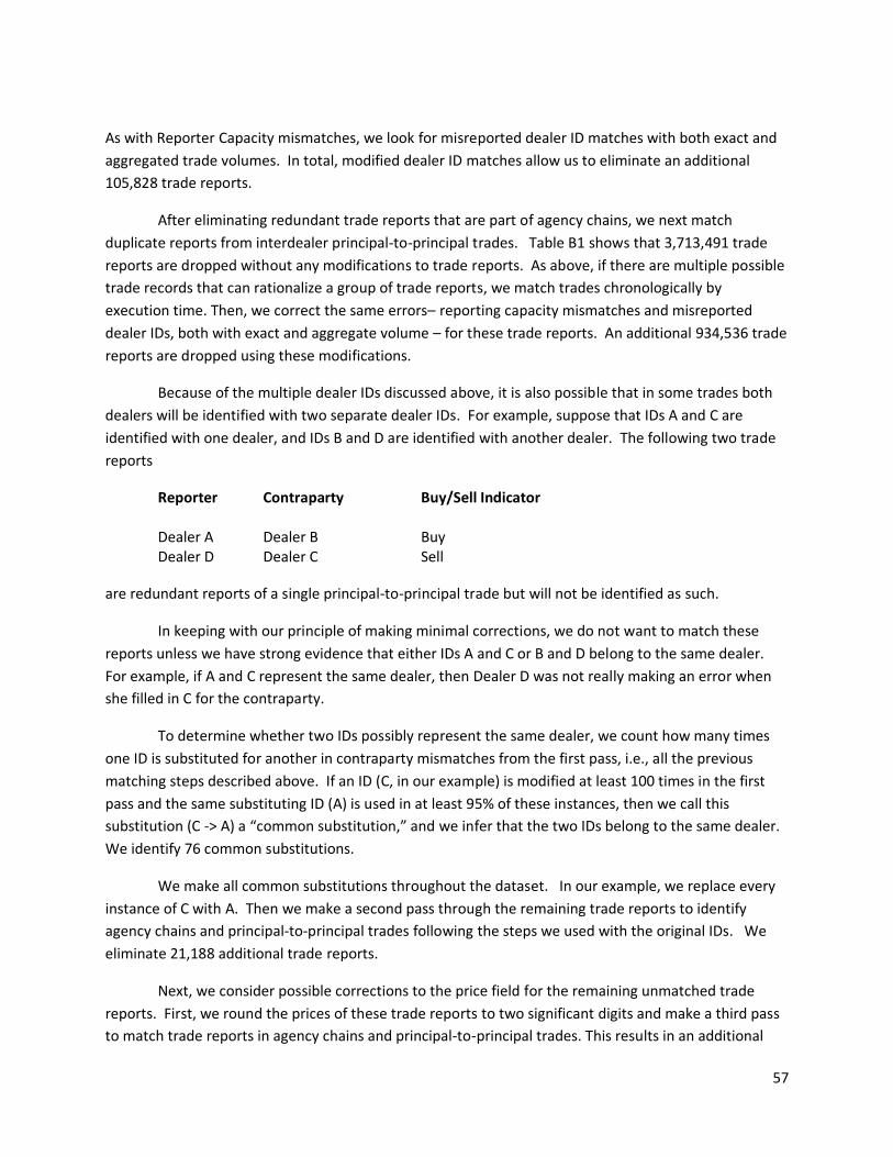
57

As with Reporter Capacity mismatches, we look for misreported dealer ID matches with both exact and

aggregated trade volumes. In total, modified dealer ID matches allow us to eliminate an additional

105,828 trade reports.

After eliminating redundant trade reports that are part of agency chains, we next match

duplicate reports from interdealer principal-to-principal trades. Table B1 shows that 3,713,491 trade

reports are dropped without any modifications to trade reports. As above, if there are multiple possible

trade records that can rationalize a group of trade reports, we match trades chronologically by

execution time. Then, we correct the same errors– reporting capacity mismatches and misreported

dealer IDs, both with exact and aggregate volume – for these trade reports. An additional 934,536 trade

reports are dropped using these modifications.

Because of the multiple dealer IDs discussed above, it is also possible that in some trades both

dealers will be identified with two separate dealer IDs. For example, suppose that IDs A and C are

identified with one dealer, and IDs B and D are identified with another dealer. The following two trade

reports

Reporter Contraparty Buy/Sell Indicator Dealer A Dealer B Buy Dealer D Dealer C Sell

are redundant reports of a single principal-to-principal trade but will not be identified as such.

In keeping with our principle of making minimal corrections, we do not want to match these

reports unless we have strong evidence that either IDs A and C or B and D belong to the same dealer.

For example, if A and C represent the same dealer, then Dealer D was not really making an error when

she filled in C for the contraparty.

To determine whether two IDs possibly represent the same dealer, we count how many times

one ID is substituted for another in contraparty mismatches from the first pass, i.e., all the previous

matching steps described above. If an ID (C, in our example) is modified at least 100 times in the first

pass and the same substituting ID (A) is used in at least 95% of these instances, then we call this

substitution (C -> A) a “common substitution,” and we infer that the two IDs belong to the same dealer.

We identify 76 common substitutions.

We make all common substitutions throughout the dataset. In our example, we replace every

instance of C with A. Then we make a second pass through the remaining trade reports to identify

agency chains and principal-to-principal trades following the steps we used with the original IDs. We

eliminate 21,188 additional trade reports.

Next, we consider possible corrections to the price field for the remaining unmatched trade

reports. First, we round the prices of these trade reports to two significant digits and make a third pass

to match trade reports in agency chains and principal-to-principal trades. This results in an additional

58

460,405 trade reports being eliminated. We make a fourth pass with truncated prices (e.g., we truncate

100.116 to 100.11, as opposed to rounding to 100.12). We eliminate additional 26,269 trade reports.

Modify or eliminate trade reports with price or volume issues

Some trade prices are vastly out of line with other prices for the bond during the same period.

To identify these prices, we first define two reference prices, before and after the trade report. The

reference prices are the median prices, weighted by volume, of the 10 trades immediately before and 10

trades immediately after the trade. If there are fewer than 10 trades in the 30 days before or after, we

use all the trades in the 30 days. A trade price is vastly out of line if the bond price differs by more than

$20 per bond in the same direction from both the before and after reference prices. When a trade is

vastly out of line, we replace it with the volume-weighted median prices for the entire 20 trades or 60-

day window. A total of 6,850 prices were replaced with the reference price.

These modifications do not necessarily correct all the prices that may be erroneous. For

example, the procedure above does not correct the price if there is not another trade report in the 60-

day window. We, therefore, drop trade reports less than the 0.01 percentile and 99.99 percentile of all

trade prices in the sample. Table B1 shows we drop 4,848 trade reports.

Next, we eliminate trades from the dataset when volume information appears erroneous.

Since, as mentioned above, all trades are self-reported, data entry errors are possible even though

TRACE monitors reported trades. We, therefore, drop trade reports less than the 0.01 percentile and

99.99 percentile of all trade volumes in the sample. Table B1 shows we drop 3,283 trade report. We

also eliminate 4,396 trade reports in which the volume of a single trade is higher than 50% of the issue

amount. Then, we eliminate 2,425 trade reports in which the volume was reported as less than $1,000.

Remaining unmatched trade reports

After the steps to assemble the data set, there are still unmatched trade reports. Recall that

every agency chain should generate at least two agency trade reports and every principal-to-principal

should generate two dealer trade reports or a single dealer-customer trade report. This implies that if

we have cleaned our dataset perfectly, there should be no unmatched agency or interdealer principal-

to-principal trade reports. In fact, we are left with 835,426 unmatched agency trade reports, of which

429,578 are sells and 405,848 are buys, and 1,360,771 unmatched interdealer principal-to-principal

trades reports, of which 585,407 are sells and 775,364 are buys. (These numbers are not shown in Table

B1).

In addition, when we examine when these unmatched trade reports occurred, we find that they

occur more frequently at the beginning of the sample period. For example, in August 2002, unmatched

agency trade reports are 47% of all agency trade reports, while by August 2006 (near the end of our

sample), it is 13%. Likewise, in August 2002, unmatched dealer trades are 27% of all trades, while by

August 2006, it is close to 3%.

There are several possible reasons why unmatched reports remain in our data.

59

1. An unmatched report may represent a trade that occurred, but the other dealer failed

to submit her own report.

2. An unmatched report may represent a trade that was modified, cancelled, or reversed,

but we cannot identify it as such. For example, Table B1 shows there are 30,724 trade

reports marked as reversals that were never matched to an earlier trade.

3. There may be two unmatched reports that describe the same trade. However, because

of differences in reporting conventions or mistakes in data entry, the reports do not

match.

If we knew why each an unmatched trade report exists, then we could process it appropriately.

For example, if a trade report were of type 1, we would like to keep it in our sample. If a trade report

were of type 2, we would like to eliminate it from our sample. If there is a group of trade reports of type

3, then one solution would keep all the buy trade reports or keep all the sell trade reports.

Unfortunately, we do not know how to distinguish among different types of unmatched trade reports.

Therefore, to check that our results are robust to the various types of possible errors, we

construct three different final trade sets: 1) keeping all unmatched agency and interdealer principal-to-

principal trades (both buy and sell), 2) dropping all unmatched agency and interdealer principal-to-

principal trades (both buy and sell), and 3) we drop all unmatched buy reports in interdealer principal-

to-principal trades, drop trade reports that are replicates of agency chains and principal-to-principal

trades, and unmatched dealer sells where the difference between execution date and reporting date is

greater than 1 day (more than 50% of these trades where 1 day). Table B1 shows that we have

dropped 2,196,197 unmatched trade reports between the first sample and third sample.

In the paper, we report estimates using the conservative sample, but we have re-run all

estimates in Table 3-11 using the moderate and aggressive samples as well. The results are similar

across these three samples and are available upon request.

Constructing the Cleaned Phases Sample

The entire dataset of cleaned bonds is not necessarily useful when evaluating the effect of

TRACE. Our empirical strategy is based on comparing a bond’s trading behavior when it changes from

non-disseminated to disseminated. If a bond does not have both disseminated and non-disseminated

trades, it will not be useful for many of our statistical tests. Many bonds are disseminated for their

entire trading history. These include bonds that belong to a FINRA Phase that are issued after the

beginning of the Phase date, and bonds that may be issued before a Phase begins but only trade after

the dissemination change date for that Phase. There are also bonds that are always non-disseminated.

These are bonds that may mature before the beginning of their Phase date as well as bonds that belong

to a Phase but never trade after the Phase begins.

Table B2 outlines the steps from Academic Cleaned Sample in Table B1 to the Cleaned Phase

Sample, the sample of bonds which exist and have zero or non-disseminated trading before the start of

a Phase and zero or disseminated trading after the start of a Phase. We begin with a list of all Phase 1,

2, 3A, and 3B bonds. There are 20,713 bonds in this list, of which 20,337 exist in the Cleaned Academic

60

TRACE Sample. They have 18,390,345 trades during our sample period. Thus, about two-thirds of the

bonds in our Cleaned Academic TRACE Sample are in our Phase list and this represents 82.4% of the

trades.

For Phases 2, 3A, and 3B, FINRA provided us with a list of bonds that began being disseminated

at the start of each of the three Phases. This list was provided in a non-electronic format where bonds

were identified with ticker symbols. Unfortunately, many ticker symbols longer than six characters were

truncated. This was a problem for firms with a four-character company ticker symbol which also issued

bonds with three-character security tickers. In particular, many GMAC bonds were truncated. Since

FINRA also provided us with coupon and maturity dates for each bond, we were able to hand-match

many of the truncated ticker symbols, but not all. The list of Phase 1 bonds was not provided by FINRA,

and we generated it ourselves. If a bond has disseminated trades before the start of Phase 2, and is not

part of the Phase 2, 3A, 3B samples or the FINRA50/120 samples, we classify it as a Phase 1 bond.

In addition to the four Phases that correspond to the FINRA dissemination dates, FINRA also

maintained two other lists of bonds, which we call the FINRA50 and the FINRA120.40 The FINRA50

represent 50 Non-Investment Grade (High-Yield) securities disseminated under Fixed Income Pricing

System (FIPS2). This list of 50 bonds changes over time with bonds both entering and exiting. FINRA

lists all of these bonds on their website and there are a total of 149 bonds that were in the FINRA50 at

some point during its existence from July 1, 2002 until July 14, 2004. The FINRA120 list is a special set of

120 investment grade rated Baa/BBB that FINRA delayed Phase 2 dissemination for. Phase 2

dissemination started on March 3, 2003 for Phase 2 bonds but started on April 14, 2003 for the

FINRA120. This special sample was created so that FINRA could conduct a controlled experiment to

study the effects of dissemination in Phase 2, contained in Goldstein, Hotchkiss, and Sirri (2007).

Table B2 explains how we went from FINRA’s list of Phase 2, 3A, and 3B bonds, and our list of

Phase 1 bonds, to our Cleaned Phase Sample. For each Phase list, we only use bonds that exist in our

Cleaned Academic TRACE Sample. Some bonds on the FINRA lists did not trade during our sample

period and thus are not in the Cleaned Academic TRACE Sample. This is shown between lines 1 and 2

under Phases 2, 3A, and 3B.

We next eliminate any bonds that also exist in the FINRA50 or FINRA120 list. Following this, we

eliminate bonds that do not exist (i.e., were not issued or matured) during the period 90 days before

until 90 days after the start of the Phase. Finally, we dropped some bonds with data problems. There

are a few bonds where FINRA report disseminated trades before the start of the Phase, or non-

disseminated trades after start of Phase. After applying these steps for each Phase list, what remains is

our cleaned sample by Phases. There is a total of 16,854 bonds in our Cleaned Phase Sample

representing 15,952,736 trades during our time period.

40 The list is available at http://www.finra.org/Industry/Compliance/MarketTransparency/TRACE/ Announcements/P117685, last accessed March 7, 2019.

61

Appendix C: NAIC Data

The National Association of Insurance Companies (NAIC) dataset we use is from Mergent FISD

available on WRDS. The NAIC requires insurance companies to self-report all securities transactions in

their financial statements. There are 63,859 bonds with 1,933,095 reported transactions in the NAIC file

over the period January 1, 2000 until December 31, 2006. Schedule D of the annual NAIC filings require

insurers to report all bond transactions in one of three categories: bonds added to the portfolio during

the calendar year and held through the end of the year, bonds deleted from the portfolio during the

calendar year that were not added in the same year, and bonds added and deleted in the same calendar

year. For each transaction, the database records the CUSIP, date, par value of the transaction, the actual

value of the transaction, if it was an addition or deletion, and a field for the counterparty involved in the

transaction. Prices are not reported but can be computed from the ratio of the value received in the

transaction to the par value of the bonds in the transaction. Importantly, the names of the insurance

companies involved in the transactions are excluded from the data.

To make the NAIC analysis comparable to the TRACE analysis, we first match our sample of NAIC

bonds with the Academic TRACE sample by CUSIP. The universe of bonds which insurance companies

trade is much larger than that reported by TRACE. 53,030 NAIC bonds representing 1,150,611 reported

transactions are not included in our Academic TRACE sample and are eliminated. Table B1 reports the

number of transactions and CUSIPs eliminated by this step.

Next, we eliminate reported transactions that are not connected to trades. The NAIC database

contains all transactions involving insurance companies’ bond portfolios, not only buy and sell

transactions, but also other transactions such as bond calls and maturities. The type of transaction is

coded in the counterparty field. We eliminate all transactions that change bond portfolio holdings that

are not buys or sells. These include the following codes: CALL, CANCEL, CONVERT, EXCHANGE, ISSUE,

MATURE, PUT, REDEEM, SINKING FUND, TAX-FREE EXCHANGE, TENDER, TRANSFER, PAYDOWN, and

REPLACE.

There are two prevalent entries in the counterparty field comprising almost 15% of the cleaned

database that required additional attention: DIRECT and VARIOUS. DIRECT may indicate a direct

placement, similar to an underwriting, or it may indicate the name of a counterparty in an actual trade.

VARIOUS is simply an ambiguous catch-all, where some records may be actual trades and some are not.

To check whether DIRECT and VARIOUS represent actual trades, we matched these NAIC records to

TRACE using the CUSIP, price, volume, and date of the transaction. For DIRECT, only about 3% of

transactions match into the TRACE dataset, while for VARIOUS only about 1% of transactions match.

Because of the problems identifying which of the DIRECT or VARIOUS transactions are actual trades, we

eliminate them along with the other codes listed above that are not buys and sells. As shown in Table

C1, all such filters eliminate 200,639 reported transactions on 8,588 different bonds.

We eliminate a small number of trades with data issues, i.e. missing prices, negative prices, etc.

We next eliminate trades with timing issues, i.e., trades that are executed before or on the bonds’

offering or after or on the bonds’ maturity date. Finally, a large fraction of NAIC transactions take place

62

on the offering and maturity dates. We believe that this is because insurance companies are large

customers of bond offerings and hold many bonds until maturity. The NAIC rules require its members to

list purchases as a transaction since the bonds are added to their portfolio. Since these transactions are

probably part of the underwriting, we do not include them as trades. If an insurance company holds the

bond until its maturity, that transaction will also be recorded by NAIC but we eliminate it. Finally, we

also exclude transactions listed on bond holidays. These screens shown in Table C1 are similar to those

applied to the TRACE dataset in Table B1.

After the screens and matching, there are 9,997 bonds and 505,753 reported transactions

(which we believe to be buys and sells) in our “clean” NAIC sample. Importantly, the NAIC time period in

Table C1 is thirty months longer than the TRACE time period in Table B1. When we restrict to the time

period July 1, 2002 until December 31, 2006, there are 9,379 bonds and 332,224 transactions, as shown

in the last three columns of Table C1.

As mentioned in Appendix A, we believe that many trades in TRACE are disaggregated by the

NAIC reporting process. When comparing the NAIC and TRACE databases, there are multiple NAIC

transactions that match to a single TRACE trade using CUSIP, date, price and counterparty, but not

volume. However, if we group NAIC transactions by CUSIP, date, price and counterparty into a single

record with a combined volume, many of these grouped NAIC trades match to a corresponding single

trade in TRACE.

There are two reasons that trades are disaggregated in NAIC. The first reason is how NAIC

requires transactions to be reported on Schedule D of the annual NAIC filing. Insurers must separately

report bonds purchased and sold in the same year from bonds purchased and held through the end of

the year. This means if an insurance company purchases $1 million par of a bond on January 1, 2001

and sells $500,000 of this before December 31, 2001 and the remaining $500,000 sometime in the

following year, under NAIC reporting instructions, this single purchase would be split into two separate

purchases of $500,000 each, reported in two different sections of Schedule D. One $500,000 purchase

would be reported in the long-term purchase reporting section, and one $500,000 purchase would be

reported in the short-term holding section.

When the NAIC database is compiled, the above trade would appear as two purchases of the

same bond occurring on the same day at the same price. In TRACE, however, the dealer who sold the

bond would report this as one $1 million trade. If we aggregate the volume of the NAIC trades that

occur in the same bond, on the same day, at the same price, the NAIC transaction would match to the

TRACE trade, as a single trade. It’s worth noting that since the insurance company sold the bond

holdings as two separate pieces of $500,000 each on two separate days, two distinct sales of $500,000

would be reported as two sales in both NAIC and TRACE.

A second reason for why a single trade may be reported as multiple trades is that distinct

subsidiaries of an insurance company may book portions of a trade to their respective division, and each

division makes its own statutory filings to the NAIC. This can occur, for instance, if part of a trade is

63

allocated to the property and casualty group and another portion allocated to the life insurance group.

In the NAIC database, this appears as two trades, while in TRACE, it appears as one trade.

We attempt to correct for these two reporting problems by grouping transactions that we

believe correspond to the same trade. Any records that share the same date, CUSIP, counterparty,

transaction type (buy or sell), and have prices within 1 cent of another are grouped and considered a

single trade. We show this grouping in Table C1. In the cleaned NAIC file, from January 1, 2000 to

December 31, 2006, the number of trades reduces from 505,753 to 412,758.

Table C1 reports the steps we took to process the raw NAIC file into our cleaned NAIC database.

We only use those bonds from the NAIC database that are also in the Cleaned Academic TRACE database

for our analysis.41 Because of the misreporting issue discussed above, Table C1 reports the total number

of transactions from the NAIC database in the column labeled “Ungrouped Trades.” It also reports an

estimate of the true number of trades by grouping transactions with identical CUSIP, date, price, and

counterparty into a single record with volume summed for the grouping. These are labeled “Grouped

Trades” in a separate column in Table C1. From July 1, 2002 to December 31, 2006, the clean NAIC

database contains 9,379 bonds. There are 332,224 ungrouped trades, which correspond to 272,133

grouped trades. This compares to 22,582,689 trades on 30,814 bonds in the Cleaned Academic TRACE

database over the same period.

To assign the bonds in NAIC to a TRACE Phase, we simply match the cleaned Phase list from

TRACE used in Table B2 to the sample of cleaned NAIC bonds. Table A2 reports the number of NAIC

CUSIPs, and both grouped and ungrouped trades in each Phase. Importantly, in Phase 1, we match 366

CUSIPs out of 388 TRACE Phase 1 CUSIPs.

As discussed in Appendix A, grouping trades does not affect our NAIC volume analysis.

However, the price standard deviation increases when we group trades. We, therefore, report the

analysis of NAIC trades both with and without grouping.

41 45,902 bonds in the NAIC database are not in the Cleaned Academic TRACE database. A large fraction of these bonds are SEC Rule 144a bonds. SEC Rule 144A bonds are not covered by TRACE during our sample period.

90-day mean for

disseminated before start of

the phase

Table 4 estimate (90-

days)

With linear and quadratic

trends specific to investment grade for each

Phase

Without Phase 1 bonds as controls (in phases 2, 3A

and 3B)

Sample matched on size, time to

maturity, and years since

issuance

90-day mean for

disseminated before start of

the phase

Table 7 estimate (90-

days)

With linear and quadratic

trends specific to investment grade for each

Phase

Without Phase 1 bonds as controls (in phases 2, 3A

and 3B)

Sample matched on size, time to

maturity, and years since

issuance

(1) (2) (3) (4) (5) (6) (7) (8) (9) (10)

Phase 1 0.301 0.020* 0.018* 0.020* 0.027** 0.560 -0.139 0.035 0.054 0.597(0.011) (0.011) (0.011) (0.012) (0.150) (0.153) (0.158) (0.363)

6.7% 6.0% 6.7% 9.0% -24.8% 6.2% 9.6% 106.5%# of Phase 1 bonds 353 345 353 348 221 221 221 215# of trades for treated Phase 1 10,618 10,585 10,618 10,599 5,450 5,450 5,450 5,385# of bond-days for treated Phase 1 43,709 42,717 43,709 43,089 2,002 2,002 2,002 1,976

Phase 1 0.368 0.024* 0.022 0.024* 0.033** 0.437 -0.085 0.035 0.046 0.391(0.014) (0.014) (0.014) (0.016) (0.111) (0.109) (0.114) (0.257)

5.5% 5.0% 5.5% 7.6% -19.5% 8.0% 10.5% 89.5%# of Phase 1 bonds 353 345 353 348 262 262 262 258# of trades for treated Phase 1 13,028 12,992 13,028 13,006 9,075 9,075 9,075 9,040# of bond-days for treated Phase 1 43,705 42,713 43,705 43,085 2,736 2,736 2,736 2,724Notes: This table reports estimates of Disseminate x Post for number of trades and daily price standard deviation for both grouped and ungrouped trades.. * significant at 10%; ** significant at 5%; *** significant at 1%

Table A1. NAIC Results for Trading Activity and Price Standard DeviationNumber of trades Price standard deviation

A. Grouped

B. Ungrouped

64

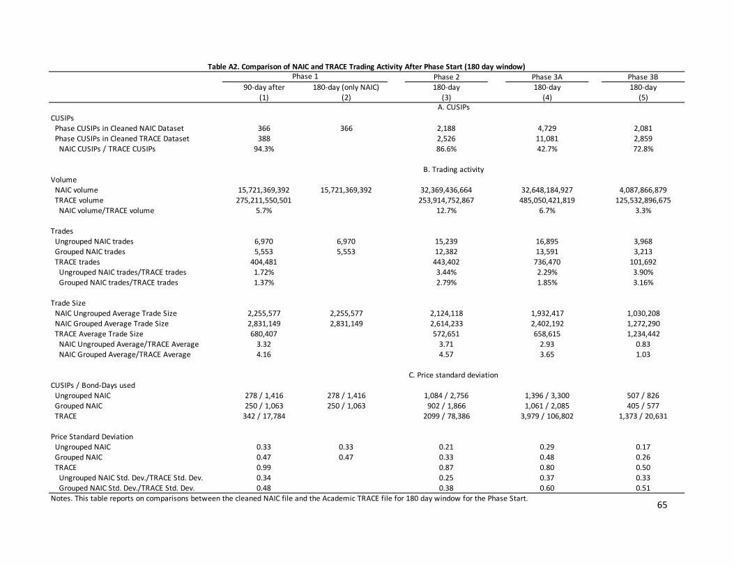
Phase 2 Phase 3A Phase 3B90-day after 180-day (only NAIC) 180-day 180-day 180-day

(1) (2) (3) (4) (5)

CUSIPsPhase CUSIPs in Cleaned NAIC Dataset 366 366 2,188 4,729 2,081Phase CUSIPs in Cleaned TRACE Dataset 388 2,526 11,081 2,859

NAIC CUSIPs / TRACE CUSIPs 94.3% 86.6% 42.7% 72.8%

VolumeNAIC volume 15,721,369,392 15,721,369,392 32,369,436,664 32,648,184,927 4,087,866,879TRACE volume 275,211,550,501 253,914,752,867 485,050,421,819 125,532,896,675

NAIC volume/TRACE volume 5.7% 12.7% 6.7% 3.3%

TradesUngrouped NAIC trades 6,970 6,970 15,239 16,895 3,968Grouped NAIC trades 5,553 5,553 12,382 13,591 3,213TRACE trades 404,481 443,402 736,470 101,692

Ungrouped NAIC trades/TRACE trades 1.72% 3.44% 2.29% 3.90%Grouped NAIC trades/TRACE trades 1.37% 2.79% 1.85% 3.16%

Trade SizeNAIC Ungrouped Average Trade Size 2,255,577 2,255,577 2,124,118 1,932,417 1,030,208NAIC Grouped Average Trade Size 2,831,149 2,831,149 2,614,233 2,402,192 1,272,290TRACE Average Trade Size 680,407 572,651 658,615 1,234,442

NAIC Ungrouped Average/TRACE Average 3.32 3.71 2.93 0.83NAIC Grouped Average/TRACE Average 4.16 4.57 3.65 1.03

CUSIPs / Bond-Days usedUngrouped NAIC 278 / 1,416 278 / 1,416 1,084 / 2,756 1,396 / 3,300 507 / 826Grouped NAIC 250 / 1,063 250 / 1,063 902 / 1,866 1,061 / 2,085 405 / 577TRACE 342 / 17,784 2099 / 78,386 3,979 / 106,802 1,373 / 20,631

Price Standard DeviationUngrouped NAIC 0.33 0.33 0.21 0.29 0.17Grouped NAIC 0.47 0.47 0.33 0.48 0.26TRACE 0.99 0.87 0.80 0.50

Ungrouped NAIC Std. Dev./TRACE Std. Dev. 0.34 0.25 0.37 0.33Grouped NAIC Std. Dev./TRACE Std. Dev. 0.48 0.38 0.60 0.51

Notes. This table reports on comparisons between the cleaned NAIC file and the Academic TRACE file for 180 day window for the Phase Start.

Table A2. Comparison of NAIC and TRACE Trading Activity After Phase Start (180 day window)Phase 1

A. CUSIPs

B. Trading activity

C. Price standard deviation

65

Affected CUSIPsAffected trade

reportsRemaining trade

reports(1) (2) (3)

Source: Academic TRACE File 41,676 37,934,432

Eliminate bonds based on characteristics Bonds unmatched to FISD by CUSIP 2,178 365,504 37,568,928 Convertible bonds 2,154 2,655,202 34,913,726 Exchangeable bonds 129 43,688 34,870,038 Other equity-linked bonds 625 210,005 34,660,033 SEC Rule 144a bonds 4,587 1,287,935 33,372,098 Bonds with missing issue size or issue size < 100,000 345 89,727 33,282,371

Eliminate trades because of self-reported errors Modifies: Trade reports matched to earlier report using sequence number 20,732 1,250,351 32,032,020 Modifies: Trade reports not matched to earlier report 0 0 32,032,020 Cancels: Trade reports matched to earlier report using sequence number 22,353 1,013,223 31,018,797 Cancels: Trade reports not matched to earlier report 0 0 31,018,797 Reversals: Trade reports matched to earlier report using nine-way match 21,278 841,108 30,177,689 Reversals: Trade reports matched to earlier report using eight-way match 8,725 87,250 30,090,439 Reversals: Trade reports matched to earlier report using eight-way match (with price rounding to two decimals)

1,137 5,694 30,084,745

Reversals: Trade reports not matched to earlier report 7,440 30,724 30,054,021

Modifying trade reports based on TRACE submission rules Add in extra trade reports for Locked-in trades 18,446 523,125 30,577,146

Eliminate trade reports with timing issues Trade reports executed earlier than July 1, 2002 956 2,195 30,574,951

Trade reports executed before bond's offering date (i.e., when-issued market) 6,770 291,840 30,283,111 Trade reports executed after bond's maturity date (i.e., bankrupt bonds) 347 93,287 30,189,824 Trade reports that occur on SIFMA holidays 20,775 802,065 29,387,759

Eliminate redundant trade reportsFirst pass: Using Original IDs

Agency chains, exact volume, original buyer-seller IDs 20,486 1,290,607 28,097,152Agency chains, aggregate volume, original buyer-seller IDs 4,131 57,314 28,039,838Agency chains, exact volume, original buyer-seller IDs, misreported agency/principal 13,139 176,744 27,863,094Agency chains, aggregate volume, original buyer-seller IDs, misreported agency/principal

1,008 3,736 27,859,358

Agency chains, exact volume, misreported original contraparty ID 7,725 94,587 27,764,771Agency chains, aggregate volume, misreported original contraparty ID 1,398 11,241 27,753,530

Interdealer principal-to-principal trade, exact volume, original buyer-seller IDs 26,350 3,713,491 24,040,039Interdealer principal-to-principal trade, aggregate volume, original buyer-seller IDs 4,509 56,605 23,983,434Interdealer principal-to-principal trade, exact volume, original buyer-seller IDs, misreported agency trade report

17,430 508,709 23,474,725

Interdealer principal-to-principal trade, aggregate volume, original buyer-seller IDs, misreported agency trade report

1,142 4,867 23,469,858

Interdealer principal-to-principal trade, exact volume, misreported original contraparty ID 17,002 353,622 23,116,236

Interdealer principal-to-principal trade, aggreage volume, misreported original contraparty ID

1,734 10,733 23,105,503

Table B1. Steps from Academic TRACE File to Cleaned Academic TRACE Sample

66

Second pass: Substitute in common dealer ID pairs from misreported original counterparty IDs

Agency chains with all modifications using substitute IDs 965 2,963 23,102,540Interdealer principal-to-principal trade with all modifications using substitute IDs 4,146 18,225 23,084,315

Third pass: rounding pricesAgency chains with all modifications using rounded prices 6,079 246,541 22,837,774Interdealer principal-to-principal trade with all modifications using rounded prices 15,306 213,864 22,623,910

Fourth pass: truncated pricesAgency chains with all modifications using truncated prices 1,360 10,117 22,613,793Interdealer principal-to-principal trade with all modifications using truncated prices 5,108 16,152 22,597,641

Modify or eliminate trade reports with price or volume issues Modify prices in trade reports that are vastly out of line 2,569 6,850 22,597,641Eliminate trade reports with price less than 0.01 percentile and greater than 99.99 percentile 284 4,848 22,592,793Eliminate trade reports with volume less than 0.01 percentile and greater than 99.99 percentile 1,564 3,283 22,589,510Eliminate trade reports with volume/issue amount ≥ 50% 1,868 4,396 22,585,114Eliminate trade reports with volume less than 1000 693 2,425 22,582,689

Cleaned Academic TRACE Sample keeping all unmatched trade reports 30,814 22,582,689Unmatched dealer buy trade reports 24,916 968,799 21,613,890Unmatched dealer sell trade reports 21,904 783,012 20,830,878Unmatched agency trade reports 15,451 444,386 20,386,492

Cleaned Academic TRACE Sample keeping unmatched dealer sell trade reports 30,728 21,613,8902,196,197

Cleaned Academic TRACE Sample dropping all unmatched trade reports 30,676 20,386,492Notes. Filters are applied sequentially. This table reports the steps from the historical TRACE file to the Clean Historical TRACE file. Other equity-linked bonds have "KNOCK", "REVERSE", "EQUITY", "LINKED", and "TBD" in the bond's FISD issue name. A seven-way match is based on CUSIP, execution date, execution time, price, quantity, buy-sell indicator, and dealer-customer indicator. A six-way match drops the execution time requirement. SIFMA holidays correspond to "Recommended Early Close" and "Recommended Full Close" dates listed at http://www.sifma.org/uploadedfiles/research/statistics/statisticsfiles/misc-us-historical-holiday-market-recommendations-sifma.pdf. In the third pass, prices are rouned to two decimal places. In the fourth pass, prices are truncated to two decimal places. We use the rounded price for all subsequent steps after the fourth pass. We define a price of a trade record to be vastly out of line if the magnitude of difference between the price of that trade record and the volume weighted median of 10 records before and 10 records after is greater than 20 per $100 par and sign of difference before and after are opossite. We require that all the 10 trades to be within the 30 days before and 30 days after. If there are fewer than 10 trades in the 30-day window,

67

CUSIPs Trade records(1) (2)

Cleaned Academic TRACE Sample (after Table B1) keeping all unmatched trade reports 30,814 22,582,689Source: FINRA list of Phase 1-3B bonds 20,713 -Bonds on both FINRA Phase list and Cleaned Academic TRACE Sample 20,337 18,390,345

Phase 1 list of Phase 1 bonds* 464 4,910,313 bonds in FINRA50 at start of phase 3 33,172 bonds do not exist as of start of phase 65 745,749 bonds do not exist for the entire period 90 days before until 90 days after start of phase 8 536 Cleaned Phase 1 Sample 388 4,130,856

Phase 2 FINRA's list of Phase 2 bonds 3,203 - Phase 2 bonds in Cleaned Academic TRACE Sample 3,016 3,111,987 bonds in FINRA50 before or at start of phase 0 0 bonds do not exist as of start of phase 265 22,283 bonds do not exist for the entire period 90 days before until 90 days after start of phase 225 155,075 Cleaned Phase 2 Sample 2,526 2,934,629

Phase 3A FINRA's list of Phase 3A bonds 13,364 - Phase 3A bonds in Cleaned Academic TRACE Sample 13,197 8,855,575 bonds in FINRA50 or FINRA120 before or at start of phase 78 651,859 bonds do not exist as of start of phase 969 181,008 bonds do not exist for the entire period 90 days before until 90 days after start of phase 1,069 280,214 Cleaned Phase 3A Sample 11,081 7,742,494

Phase 3B FINRA's list of Phase 3B bonds 3,682 - Phase 3B bonds in Cleaned Academic TRACE Sample 3,660 1,512,470 bonds in FINRA50 or FINRA120 before or at start of phase 26 58,881 bonds do not exist as of start of phase 643 257,195 bonds do not exist during the period 90 days before until 90 days after start of phase 132 51,637 Cleaned Phase 3B Sample 2,859 1,144,757

Total Cleaned Phase 1-3B Sample 16,854 15,952,736

Table B2. Steps from FINRA's Phase Listings to Cleaned Phase Sample

Notes. This table reports the match between the Cleaned Academic TRACE file and FINRA's Phase Listings. Not all bonds in the TRACE Academic Sample are classified in a FINRA Phase. Excluded bonds are those issued after 7/1/02 that are always disseminated and those that mature before 2/7/05 that are never disseminated. We construct the Phase 1 list by including all bonds with disseminated trades before Phase 2 that are not on the FINRA Phase 2, 3A, or 3B lists. The Phase 2, 3A, and 3B lists were obtained directly from FINRA. The FINRA50 and FINRA120 lists are from www.finra.org. Bonds in FINRA's Phase lists that are not in the Cleaned Academic TRACE Sample have either never traded during the sample period or have been eliminated due to cleaning process in Table A1.

68

CUSIPsUngrouped trades

Grouped trades CUSIPs

Ungrouped trades

Grouped trades

Original Source: NAIC Transactions File 63,859 1,933,095 1,490,831 50,968 1,341,769 1,032,125

Match NAIC Bonds with Cleaned Academic TRACE Sample keeping all unmatched trade recordsCUSIP not found in Cleaned Academic TRACE Sample keeping all unmatched trade records

53,030 1,150,611 884,359 40,454 819,448 629,630

Eliminate transactions which are not tradesNon-trade indicated by counterparty field entry (calls, converts, etc.)

8,588 200,639 145,052 8,124 155,205 106,278

Eliminated trades with timing issuesTrades executed on or before bond's offering date 3,813 53,580 29,053 2,000 20,474 11,856Trades executed on or after bond's maturity date 556 1,026 944 556 1,026 944Trades executed on weekend or SIFMA Holiday 5,086 20,131 17,661 3,789 11,963 10,449Post July 2002 trades executed on days with no TRACE trades**

4 8 7 4 8 7

Eliminate trades with price and volume issuesTrades with price less than 0.01 percentile and greater than 99.99 percentile

276 564 376 271 559 371

Trades with volume/issue amount >= 50% 202 472 318 126 294 191Trades with volume less than 1000 176 311 303 158 270 265

Cleaned NAIC Sample 9,997 505,753 412,758 9,379 332,224 272,133Notes: Filters are applied sequentially. The CUSIPs column gives total number of CUSIPs eliminated from the database by adding that row's filter. The trades column gives totalnumber of observations eliminated by adding that row's filter.**On June 11, 2004, the SEC declared a holiday when President Reagan died. Grouping is done if the difference in Price is <= |0.01| and the day, counterparty, insurer type, and buy or sell are equal.

Table C1. Steps from Historical NAIC File to Cleaned Academic SampleJanuary 1, 2000 - December 31, 2006 July 1, 2002 - December 31, 2006

69

70

References

Acharya, V., R. Engle, S. Figlewski, A. Lynch, and M. Subrahmanyam. 2009. “Chapter 11: Centralized

Clearing for Credit Derivatives.” In Restoring Financial Stability: How to Repair a Failed System,

Wiley and NYU Stern, 2009.

Akins, B. 2018. “Financial Reporting Quality and Uncertainty about Credit Risk among the

Ratings Agencies.” The Accounting Review, 93(4): 1-22.

Alexander, G., A. Edwards, and M. Ferri. 2000. “The Determinants of Trading Volume in High-yield

Corporate Bonds.” Journal of Financial Markets, 3, 177-204.

Asquith, P., A. Au, T. Covert, and P. A. Pathak. 2013. “The Market for Borrowing Corporate Bonds.”

Journal of Financial Economics, 107, 155-182.

Bessembinder, H. and W. Maxwell. 2008. “Markets: Transparency and the Corporate Bond Market.”

Journal of Economic Perspectives, 22 (2), 217-234.

Bessembinder, H., W. Maxwell, and K. Venkataraman. 2006. “Market Transparency, Liquidity

Externalities, and Institutional Trading Costs in Corporate Bonds.” Journal of Financial

Economics, 82, 251-288.

Bessembinder, H., S. Jacobsen, W. Maxwell and K. Venkataraman 2018, “Capital Commitment and

Illiquidity in Corporate Bonds.” Journal of Finance, 73: 1615-1661.

Biais, B. and R. Green. 2018. “The Microstructure of the Bond Market in the 20th Century.” Working

paper, Toulouse University.

Biais, B., L. Glosten, and C. Spatt. 2005. “Market Microstructure: A Survey of Microfoundations,

Empirical Results, and Policy Implications.” Journal of Financial Markets, 8(2), 217-264.

Bloomfield, R. and M. O’Hara. 1999. “Market Transparency: Who Wins and Who Loses?” The Review of

Financial Studies 12 (1), 5-35.

Bravo, R. A. 2003. “Corporate-Bond Pricing System May Be Too Open, Critics Say.” Wall Street Journal,

April 15.

Brancaccio, G., D. Li, and N. Schurhoff. 2017. “Learning by Trading: The Case of the U.S. Market for

Municipal Bonds.” Unpublished paper. Princeton University.

Corwin, S. A. and P. Schultz. 2012. “A Simple Way to Estimate Bid-Ask Spreads from Daily High and Low

Prices.” Journal of Finance 67 (2), 719-760.

71

Decker, M. 2007. “FINRA’s TRACE and the U.S. Corporate Bond Market.” Presentation to Securities

Industry and Financial Markets Association. September 11.

Di Maggio, M., A. Kermani, and Z. Song. 2017. “The value of trading relations in turbulent times.” Journal

of Financial Economics, 142 (2), 266-284.

Dow Jones. 2002. “NASD to Increase Bond-Trade Data Available to Public.” Dow Jones Newswires,

November 22.

Duffie, D. 2012. Dark Markets: Asset Pricing and Information Transmission in Over-the-Counter Markets.

Princeton University Press.

Dugalic, A. 2017. “Corporate Bond Market Post-Trade Transparency and Dealer Behavior.” Unpublished

paper. Stanford University.

Economist. 2011. “Derivatives: Unlucky for Some. Proposed Rules on Taming Swaps Markets are Proving

Controversial.” March 3.

Edwards, A., L. Harris, and M. Piwowar. 2007. “Corporate Bond Market Transparency and Transaction

Costs.” Journal of Finance, 62 (3), 1421-1451.

Financial Services Forum, Futures Industry Association, International Swaps and Derivatives Association,

and Securities Industry and Financial Markets Association, 2011. “Comment Letter RE: Phase-In

Schedule for Requirement for Title VII of Dodd-Frank Act.” May 4. Available at:

http://www.sec.gov/comments/s7-16-10/s71610-177.pdf, Last accessed, March 7, 2019.

French, K., M. Baily, J. Campbell, J. Cochrane, D. Diamond, D. Duffie, A. Kashyap, F. Mishkin, R. Rajan, D. Scharfstein, R. Shiller, H. S. Shin, M. Slaughter, J. Stein, and R. Stulz. 2010. The Squam Lake Report: Fixing the Financial System. Princeton University Press.

Gemmill, G. 1996. “Transparency and Liquidity: A Study of Block Trades on the London Stock Exchange

under Different Publication Rules.” Journal of Finance 51 (5), 1765-1790.

Green, R., B. Hollifield, and N. Schürhoff. 2007a. “Financial Intermediation and the Costs of Trading in an

Opaque Market.” Review of Financial Studies 20 (2), 275-314.

Green, R., B. Hollifield, and N. Schürhoff. 2007b. “Dealer Intermediation and Price Behavior in the

Aftermarket for New Bond Issues.” Journal of Financial Economics, 86, 643-682.

72

Grundy, B. and M. McNichols. 1989. “Trade and the Revelation of Information through Prices and Direct

Disclosure.” Review of Financial Studies 2 (4), 495-526.

Goldstein, M., E. Hotchkiss, and E. Sirri. 2007. “Transparency and Liquidity: A Controlled Experiment on

Corporate Bonds.” Review of Financial Studies 20 (2), 235-273.

Goldstein, M. and E. Hotchkiss. 2008. “Dealer Behavior and the Trading of Newly Issued Corporate

Bonds.” Unpublished paper. Boston College.

Goldstein, Michael A. and Hotchkiss, Edith S. 2017. “Providing Liquidity in an Illiquid Market: Dealer

Behavior in U.S. Corporate Bonds.” Unpublished paper. Boston College.

Hendershott, T., D. Li, D. Livdan, and N. Schurhoff. 2017. “Relationship Trading in OTC Markets.”

Unpublished paper. University of California.

Jamieson, D. 2006. “Report card for TRACE a mixed bag.” InvestmentNews, July 24.

Ketchum, G. R. “Speech: Bond Dealers Association Annual Conference.” Chicago, IL, October 11, 2012.

Available at: http://www.finra.org/newsroom/speeches/ketchum/p187314. Last accessed:

March 7, 2019.

Learner, H. 2011. “An Examination of Transparency in European Bond Markets.” CFA Institute, October,

Vol. 2011(5). Available at: https://www.cfainstitute.org/en/advocacy/policy-positions/an-

examination-of-transparency-in-european-bond-markets. Last accessed: March 7, 2019.

Levitt, A. 1999. “Testimony to the U.S. Congress House of Representatives House Subcommittee on

Finance and Hazardous Materials.” March 18. Available at:

http://www.sec.gov/news/testimony/testarchive/1999/tsty0499.htm. Last accessed: March 7,

2019.

Li, D. and N. Schurhoff. 2019. “Dealer Networks.” Journal of Finance, 74: 91-144

Madhavan, A. 1995. “Consolidation, Fragmentation, and the Disclosure of Trading Information.” Review

of Financial Studies 8 (3), 579-603.

Mullen, D. 2004. “Relating to Proposed Amendments to TRACE Rule 6250 and Related TRACE Rules to Disseminate Transaction Information on All TRACE-Eligible Securities and Facilitate Dissemination.” Letter from Bond Market Association to SEC, July 23.

Naik, N., Neuberger, A., and S. Viswanathan. 1999. “Trade Disclosure Regulation in Markets with

Negotiated Trades.” Review of Financial Studies 12 (4), 873-900.

73

NASD. 2005. “NASD’s Fully Implemented `TRACE’ Brings Unprecedented Transparency to Corporate

Bond Market.” February 7. Available at: http://www.finra.org/Newsroom/

NewsReleases/2005/P013274, Last accessed: March 7, 2019.

NASD. 2006. “NASD Response to European Commission; Letter in Response to EU Markets in Financial

Instruments Directive (MiFiD) Call for Evidence on Pre- and post-trade transparency provisions

requested June 12, 2006.” Available at:

http://ec.europa.eu/internal_market/securities/docs/isd/consultation_mifid/nasd_en.pdf, Last

accessed: August 29, 2013.

Nazareth, A. L. 2004. “Testimony before the United States Senate Committee on Banking, Housing, and

Urban Affairs.” Available at: http://www.sec.gov/news/testimony/ts061704aln.htm, Last

accessed: March 7, 2019.

Pagano, M. and A. Roell. 1996. “Transparency and Liquidity: A Comparison of Auction and Dealer

Markets with Informed Trading.” Journal of Finance 51 (2), 579-611.

Schultz, P. 2012. “The Market for New Issues of Municipal Bonds: The Roles of Transparency and Limited

Access to Retail Investors.” Journal of Financial Economics, 106, 492-512.

Securities Industry and Financial Market Association (SIFMA), 2013. “Table 1.1 US Corporate Average

Daily Trading Volume by Type and Rating.” Available at: http://www.sifma.org/

research/statistics.aspx. Last accessed, July 25, 2013.

Shenn, J. and D. Scheer. 2009. “FINRA Seeks to Amass Asset-Backed Bond Data on Trace.” October 1,

Bloomberg.

TRACE Factbook. 2005. National Association of Securities Dealers. Available at:

http://www.finra.org/Industry/Compliance/MarketTransparency/TRACE/FactBook/. Last

accessed: March 7, 2019.

Vames, S. 2003. “NASD Expands Bond-Price Reports – Data on Corporate Issues Becomes More

Transparent.” Wall Street Journal, March 4.