the effects of neighboring, social networks, and .../67531/metadc801962/m2/1/high... · soto,...
TRANSCRIPT

THE EFFECTS OF NEIGHBORING, SOCIAL NETWORKS, AND COLLECTIVE EFFICACY ON CRIME
VICTIMIZATION: AN ALTERNATIVE TO THE SYSTEMIC MODEL
Anthony Jaime Soto, B.S., M.P.A., M.A.
Dissertation Prepared for the Degree of
DOCTOR OF PHILOSOPHY
UNIVERSITY OF NORTH TEXAS
May 2015
APPROVED:
Gabriel Ignatow, Major Professor Philip Yang, Committee Member Adam Trahan, Committee Member George Yancey, Committee Member Daniel Rodeheaver, Chair of the
Department of Sociology Art Goven, Dean of the College of
Arts and Sciences Mark Wardell, Dean of the Toulouse
Graduate School
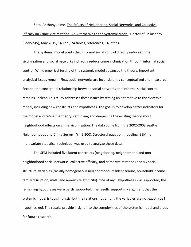
Soto, Anthony Jaime. The Effects of Neighboring, Social Networks, and Collective
Efficacy on Crime Victimization: An Alternative to the Systemic Model. Doctor of Philosophy
(Sociology), May 2015, 140 pp., 24 tables, references, 143 titles.
The systemic model posits that informal social control directly reduces crime
victimization and social networks indirectly reduce crime victimization through informal social
control. While empirical testing of the systemic model advanced the theory, important
analytical issues remain. First, social networks are inconsistently conceptualized and measured.
Second, the conceptual relationship between social networks and informal social control
remains unclear. This study addresses these issues by testing an alternative to the systemic
model, including new constructs and hypotheses. The goal is to develop better indicators for
the model and refine the theory, rethinking and deepening the existing theory about
neighborhood effects on crime victimization. The data come from the 2002-2003 Seattle
Neighborhoods and Crime Survey (N = 2,200). Structural equation modeling (SEM), a
multivariate statistical technique, was used to analyze these data.
The SEM included five latent constructs (neighboring, neighborhood and non-
neighborhood social networks, collective efficacy, and crime victimization) and six social
structural variables (racially homogeneous neighborhood, resident tenure, household income,
family disruption, male, and non-white ethnicity). One of my 9 hypotheses was supported; the
remaining hypotheses were partly supported. The results support my argument that the
systemic model is too simplistic, but the relationships among the variables are not exactly as I
hypothesized. The results provide insight into the complexities of the systemic model and areas
for future research.

ii
Copyright 2015
by
Anthony Jaime Soto

iii
ACKNOWLEDGEMENTS
This dissertation would not have been possible without the support and guidance from
many people. Although it is impossible to acknowledge every one individually, I am indebted to
all of you for making this dream possible. I am particularly grateful to my dissertation
committee. I am thankful to Gabriel Ignatow, PhD for his mentorship throughout my doctoral
program. I am also thankful to Adam Trahan, PhD and George Yancey, PhD for their
contributions to my dissertation. I extend a very special thanks to Philip Yang, PhD for his
consistent kindness and statistical expertise. My deepest gratitude and sincerest appreciation
to my bosses, Timothy Brady, PhD and Michael Henry, JD at the United States Department of
Health and Human Services, Office of Inspector General, Office of Evaluation and Inspections
for their continued and overwhelming support. Thank you James McGrath, JD for being part of
my family and standing by my side. Thank you Albert Guerrero for encouraging me and
supporting my initial decision to pursue a PhD. Thanks to my friends and colleagues in the
graduate program, I would not have been able to get through this program without their
friendship and camaraderie. Our adventures will forever be in my heart. Finally, thanks to my
parents, Mario and Diane, with whom I share this accomplishment.
This dissertation is dedicated to the memory of Mage Jaime, my ultimate cheerleader in
life, and Kevin Yoder, PhD. I am deeply honored to have known both of you.

iv
TABLE OF CONTENTS
ACKNOWLEDGEMENTS……………………………………………………………………………………………………………..iii
LIST OF TABLES……………………………………………………………………………………………………………………..….vii
LIST OF FIGURES………………………………………………………………………………………………………………………..ix
Chapters
1. INTRODUCTION
Introduction……………………………………………………………………………………………………….1
Research Problem……………………………………………………………………………………………….2
Purpose of the Study…………………………………………………………………………………………..2
Significance of Study……………………………………………………………………………………..……4
Dissertation Overview…………………………………………………………………………………………5
2. REVIEW OF THE LITERATURE
Social Disorganization Theory …………………………………………………………………………….7
The Systemic Model of Neighborhood Crime …………………………………………………….9
Social Structural Characteristics………………………………………………………………………..12
Problems with the Empirical Testing of the Systemic Model…………………………….15
Outstanding Issues with the Systemic Model……………………………………………………30
3. CONCEPTUAL FRAMEWORK
Introduction……………………………………………………………………………………………………..33
Defining Neighboring………………………………………………………………………………………..33
My Conceptual Framework……………………………………………………………………………….37
The Current Study…………………………………………………………………………………………….42

v
Research Questions ………………………………………………………………………………………….44
Hypotheses……………………………………………………………………………………………………….44
4. DATA AND METHODS
Introduction……………………………………………………………………………………………………..48
Data Source………………………………………………………………………………………………………48
Variables and Measures……………………………………………………………………………………49
Data Screening………………………………………………………………………………………………….55
Data Analysis Plan…………………………………………………………………………………………….55
5. RESULTS
Introduction……………………………………………………………………………………………………..60
Descriptive Statistics…………………………………………………………………………………………60
Bivariate Correlations……………………………………………………………………………………….67
Confirmatory Factor Analysis……………………………………………………………………………72
Full Measurement Model………………………………………………………………………………….90
Structural Equation Modeling……………………………………………………………………………97
Summary of Hypotheses Tested……………………………………………………………………..106
6. DISCUSSION AND CONCLUSION
Summary of Findings and Discussion………………………………………………………………111
Implications of the Findings……………………………………………………………………………115
Limitations and Recommendations for Future Research………………………………..118
Appendix
CORRELATION MATRICES FOR VARIABLES USED IN ANALYSIS ……………………....121

vi
REFERENCES………………………………………………………………………………………………………………………….126

vii
LIST OF TABLES
Table 1 Social Networks and Informal Social Control Measures Used in Selected Prior Research………………………………………………………………………………………………………………………………….16
Table 2 Descriptive Statistics of the Sample, Seattle Adults, 2002-2003…………………………………..61
Table 3 Descriptive Statistics of the Social Structural Variables………..………………………………………62
Table 4 Percentage Distribution of Social Network Activities……………………………………………………63
Table 5 Percentage Distribution of Neighboring Activities……………………………………………………….64
Table 6 Percentage Distribution of Collective Efficacy Activities………………………………………………66
Table 7 Descriptive Statistics for Crime Victimization Variables.………………………………………………67
Table 8 Correlations Matrix for Social Structural Variables………………………………………………………68
Table 9 Correlation Matrix for Social Network Variables………………………………………………………….69
Table 10 Correlations for Neighboring Variables……………………………………………………………………..70
Table 11 Correlation Matrix for Collective Efficacy Variables…………………………………………………..71
Table 12 Correlation Matrix for Crime Victimization………………………………………………………………..72
Table 13 Parameter Estimates for Social Networks………………………………………………………………….76
Table 14 Goodness-of-Fit Statistics for Social Networks…………………………………………………………..77
Table 15 Parameter Estimates for Neighboring………………………………………………………………………..80
Table 16 Goodness-of-Fit Statistics for Neighboring…………………………………………………………………81
Table 17 Parameter Estimates for Collective Efficacy……………………………………………………………….84
Table 18 Goodness-of-Fit for Collective Efficacy……………………………………………………………………….85
Table 19 Parameter Estimates for Crime Victimization…………………………………………………………….88
Table 20 Goodness-of-Fit Statistics for Crime Victimization……………………………………………………..89
Table 21 Parameters of the Measurement Model, Standardized Path Coefficient, Z Values, Composite Reliability, Average Variance Extracted, Variance Extracted, and Highest Shared Variance…………………………………………………………………………………………………………………………………..92

viii
Table 22 Correlations Among Latent Constructs………………….…………………………………………………..95
Table 23 Parameter Estimates for Generic and Revised SEM………………………………………………….102
Table 24 Goodness-of-Fit Statistics for Generic and Revised SEM………………………………………….105

ix
LIST OF FIGURES
Figure 1 The systemic model of neighborhood crime……………………………………………………………….1
Figure 2 Sampson and Groves’ (1989) casual model……………………………………………………………..…20
Figure 3 Hypothetical model………….………………..………………………………………………………………………44
Figure 4 Generic measurement model for social networks.…………………………………………………….74
Figure 5 Revised measurement model for social networks……………….…………………………………….75
Figure 6 Generic measurement model for neighboring…………………………………………………………..78
Figure 7 Revised measurement model for neighboring……………………………………………………………81
Figure 8 Generic measurement model for collective efficacy………………………………………………….82
Figure 9 Revised measurement model for collective efficacy………………………………………………….83
Figure 10 Generic measurement model for crime victimization………………………………………………86
Figure 11 Revised measurement model for crime victimization………………………………………………88
Figure 12 Measurement model for all constructs with parameter estimates and error terms………………………………………………………………………………………………………………………………………94
Figure 13 My Empirical model………………………………………………………………………………………………….96
Figure 14 Generic structural equation model…………………………………………………………………………100
Figure 15 Revised structural equation mode………………………………………………………………………….101

1
CHAPTER 1
INTRODUCTION
Introduction
Social disorganization theory (Shaw and McKay, 1942) is one of the oldest and most
prominent theories in the ecological explanation of neighborhood crime and delinquency.1
Contemporary development of the theory is most influenced by the systemic model of
neighborhood crime (Bellair and Browning, 2010; Kubrin, Stucky, and Krohn, 2009), with its
emphasis on social networks, family, and friendship and their capacity for generating informal
social control through socialization. The systemic model posits that informal social control
directly reduces crime and social networks indirectly reduce crime through informal social
control (see Figure 1).
Figure 1 The Systemic Model of Neighborhood Crime
1 The creation and maintenance of social order is a long-standing area of inquiry for sociologists. Studies have generally developed an interest in integrating macro-level processes with more micro-level dynamics (see Durkheim, 1883; Tonnies, 1887). In addition, studies on social order share a systemic focus on the concept of control as a mechanism to create and preserve social groups and organize their patterns of interactions (see Durkheim, 1893; Coleman, 1990). These two avenues of inquiry on social order have influenced studies on the social organization of urban settings. The ecological framework provided the foundation for studies seeking to explain the conditions by which neighborhoods develop organizing principles and maintain their collective dimensions. Neighborhoods are connected to a broader social structure, which influences patterns of residence and the integration of these spaces into normative systems.

2
Research Problem
While empirical testing of the systemic model has increased our understanding of the
theory, important analytical issues remain unaddressed. First, social networks are inconsistently
conceptualized and measured. The variation in conceptualization and measurement for social
networks may account for inconsistent findings in the literature. For example, studies may be
measuring the same concept, different dimensions of the same concept, or entirely different
concepts. Second, the conceptual relationship between social networks and informal social
control remains unclear (e.g., how social networks differ from and represent an improvement
over informal social control is still not completely understood). Hence, many studies still
conduct partial tests of the systemic model without testing the relationship between social
networks and informal social control. Resolution of these issues is important for the theoretical
development of the systemic model, because some scholars have questioned the role of social
networks and the significance of the association between social networks and informal social
control (Sampson, 2002; Morenoff et al., 2001). Before developing new theories, we need to
clarify conceptual ambiguity and improve measurement in order to properly test the existing
theory.
Purpose of the Study
The purpose of the study is to test an alternative to the systemic model. My alternative
model addresses the important analytical issues within the systemic model. To address
conceptual confusion, I make distinctions between concepts and clarify their relationships. The
concepts in my model include neighboring, social networks, collective efficacy, and crime

3
victimization. Neighboring refers to supportive social acts and neighborhood attachment, and is
a new addition to the model. Social networks are conceptualized as resident participation in
neighborhood organizations. Collective efficacy refers to social cohesion among neighbors
combined with their willingness to intervene. While collective efficacy is the action component
in my model, neighboring and social networks are the resource and social capital generating
components. By distinguishing between neighboring and social networks my model, I address
the inconsistencies with measurement. For each concept in my model, I develop indicators that
are clearly distinguishable from each other. I am translating my concepts into measures that
directly tap the hypothesized constructs.
Additionally, my alternative model examines the relationship between all the concepts,
testing the theory to see if empirical distinctions exist, based on the data. I hope to provide
clarity to the inconsistent frameworks and measurement approaches in the literature.
To address incomplete testing of the systemic model, my alternative model is a
complete test of the theory, but also I offer a new construct to the model. I will examine the
relationships between all the constructs and test the hypothesized relationships. Therefore, my
goal is not only to develop better indicators for concepts in an alternative model, but also to
test and refine the theory.
This study tests an alternative to the systemic model in a sample of Seattle, Washington
residents. Many studies are based in Chicago, Illinois, which is characterized, at least
historically, by high rates of segregation, disadvantage, and crime. Seattle has not experienced
the extreme levels of poverty or racial segregation as Chicago. Therefore, the study allows me
to test the theory (of the systemic model) with new and different data. By testing the theory in

4
a new context, we can improve our understanding of the theory and its relevance in the 21st
century. The implications of this study are important for improving neighborhood relations and
crime prevention strategies.
Significance of This Study
The concept of social networks has long been used to study correlates of social order
and crime in neighborhoods. Its longevity represents the important theoretical association
between patterns of affiliation and the development of individual and social self-regulatory
abilities. Moreover, patterns of exchange are consistently used as a mechanism to bridge the
macro-level factors of the social structure and micro-level dynamics of social control. Coleman
argued that sociology should “take into account not only system behavior, but also individual
actions as proper phenomena for study and see them as closely intertwined (…) individual
actions generate system behavior as well as system properties that, in turn, affect individual
actions” (1994, p. 34).
There is debate about the relationship between social networks and neighborhood
crime victimization. Some scholars, such as Bursik and Venkatesh, continue to emphasize, in
different ways, the significance of social networks in the organization of certain neighborhoods.
Other scholars, such as Sampson (2012), say that social networks and social exchanges are not
required to explain patterns of crime victimization. These scholars argue that research should
focus on share expectations and informal social control.
Quantitative researchers operationalize informal social control as an individual-level
covariate measuring the residents’ willingness to intervene - or the expectation that neighbors

5
would intervene (referred to as collective efficacy) - in a given set of minor disruptions of public
order. While this formulation is criticized on several theoretical and methodological grounds
(Taylor, 2002), it has become the standard in many empirical studies (Sampson, Morenoff, and
Gannon-Rowley, 2002; Warner, Leukefeld, and Kraman, 2003; Reisig and Cancino, 2004).
Overall, quantitative and qualitative studies have produced mixed results about the relationship
between social networks and informal social control, and their relationship to crime
victimization.
The mixed results are, in large part, due to the lack of more robust measures of both
social networks and informal social control, and confusion over these mechanisms (Carr, 2003).
Thus, one objective of this study is to test and develop theoretically driven measures for social
networks and test collective efficacy measures. My approach refines existing methods for social
network measurement; it moves one step further by integrating the useful elements of existing
theories in the literature. Further, this study clarifies the confusion about the relationship
between social networks and collective efficacy. By refining and testing the systemic model, this
study rethinks and deepens existing theories about neighborhood effects on crime
victimization.
Dissertation Overview
The dissertation is divided into six chapters. Chapter 1 provides an introduction of the
systemic model of neighborhood crime, the purpose of the study, and the significance of the
study. Chapter 2 provides a literature review, providing a conceptual and empirical overview of
topics that are central to the analysis, including social disorganization theory and the systemic

6
model. The focus of the literature review is to identify gaps and situates my study within the
context of the existing literature. Chapter 3 provides a conceptual framework for the study,
including my research questions and hypotheses. Chapter 4 describes the methodology and
data analysis used for this project. Chapter 5 includes the results of my analysis, including
results from my confirmatory factor analysis and structural equation modeling. Chapter 6
provides a discussion and conclusion, addresses the implications of this research, limitations to
the study, and possibilities for future research.

7
CHAPTER 2
REVIEW OF THE LITERATURE
Social Disorganization Theory
Shaw and McKay formulated (1942) the original social disorganization theory of
neighborhood crime.2, 3 They systemically applied the zonal model by Park and Burgess (1925)
to the study of deviant behavior and demonstrated that crime rates can be mapped on top of
the urban concentric circles.4 They found that three neighborhood level factors - low
socioeconomic status, ethnic heterogeneity, and resident mobility - led to the disruption of
community social organization, which in turn, accounted for variations in delinquency and
crime rates. They concluded that neighborhoods characterized by these three factors were also
plagued by a host of other social problems, including tuberculosis and low birth weights. Thus,
neighborhood characteristics and deviance appeared together and were seemingly related.
They also found that delinquency rates were not evenly distributed across the city. Delinquency
rates remained fairly stable among Chicago’s neighborhoods despite dramatic changes in the
ethnic and racial composition within these neighborhoods. This implied that, crime and 2 It is generally understood that W. I. Thomas originated the concept of social disorganization. Thomas and Znaniecki (1927: 1128) explained that social disorganization was a “decrease of the influence of existing social rules of behavior upon individual members of the group.” 3 Park and Burgess (1925) developed a model that illustrated the relationship between ecology and social disorganization. With backgrounds in human ecology, they viewed cities as analogous to the natural ecological communities of plants and animals. Using the imagery from ecological studies of plants, the growth of a city was like ecological competition (just as plants and animals compete for space and existence, there is social ecology where humans compete for desirable space – referred to as ‘biotic order’). This orientation is best reflected in Burgess (1925) concentric zone theory of urban structure. Cities expand in zones from their core and each zone, as it expands, is associated with different environmental characteristics. A second set of social dynamics existed, referred to as ‘moral order,’ and was interdependent with the ‘biotic order.’ Within the moral order, residential life is shaped by cultural and symbolic factors that affect the neighborhoods in which humans are a part of. 4 Shaw and McKay (1969) created a dataset containing the home addresses, ages, gender, and the offenses of adolescents referred the Cook County Juvenile Courts, the Cook County Boys’ Court, and the Cook County Jail from 1900 through 1965. They plotted nearly 90,000 court referrals by hand on maps of the city. The rates of delinquency were computed on the basis of census tracts. Their conclusions were based on visual inspections of these maps and rudimentary statistics.

8
delinquency are linked to social conditions, not solely linked to the ethnic composition of the
residents.
Their approach examined how macro-level structural processes detrimentally impact
neighborhood dynamics and the ability of a neighborhood to regulate itself through the use of
informal social controls.5 Poverty, heterogeneity, and rapid population turnover were thought
to reflect, at the neighborhood-level, the larger processes of urbanization, industrialization, and
social change. Delinquency and crime rates were related to the same ecological processes that
produced socioeconomic structures in urban areas (see Bursik, 1986). Specifically, these three
neighborhood factors were thought to undermine personal ties, voluntary associations, and
local institutions, which in turn were hypothesized to weaken the infrastructure necessary for
socialization and social control. Social control was an instinctive property that grew out of
strong ties between community members, representing the ability of a community to compel
members to conform to social norms and prioritized communal interests. Neighborhoods that
were less prone to develop patterns of self-regulation were labeled as socially disorganized.
However, limitations existed with Shaw and McKay’s (1942) model. Some of the
deficiencies related to theory. For example, Shaw and McKay did not clearly differentiate
among social disorganization, its causes, and its consequences. Other deficiencies related to
measurement. Researchers struggled with how to best define and capture neighborhood and
social disorganization. For some neighborhoods, what looked like disorganization may just have
been social organization of a different kind or type (see Suttles, 1968). For example, Whyte
(1943) discovered, through extensive fieldwork, an intricate pattern of social ties embedded
5 Thomas and Znaniecki (1927) and Wirth (1938) were also equally important influences, who argued that ethnic heterogeneity, along with size and density, weakened social integration within communities.

9
within the social structure of a low-income urban neighborhood. There were organized gangs
and integration of illegal markets within the routines of everyday life. Furthermore, Shaw and
McKay did not develop the notion of social relations or paid little attention to patterns of inter-
personal or institutional affiliations. Many of the neighborhoods studied by Shaw and McKay
were undergoing historic social change that ultimately ended by the 1950s (Bursik and Webb,
1982). Although initially embraced, this theory created substantial confusion and was ultimately
rejected. By the end of the 1970s, social disorganization underwent theoretical and empirical
development.6 For example, theorists defined social disorganization as “the inability of a
neighborhood to achieve the common goals of its residents and maintain effective social
controls” (Kornhauser, 1978, p. 63). Research also began to uncover the factors that mediate
the relationship between neighborhood structural characteristics and crime.
The Systemic Model of Neighborhood Crime
Recent theory has coalesced around the systemic model with its emphasis on family,
friendship, and neighbor networks of affiliation and their capacity for generating (prosocial)
informal [social] control through the process of primary and secondary socialization (see
Kasarda and Janowitz, 1974; Bursik and Grasmick, 1993).7 The thesis is that large and
interconnected networks (familial and associational networks) increase the likelihood that
residents take action for the mutual benefit of the neighborhood. Social networks are the
6 There were at least five efforts to clarify the assumptions of the Shaw and McKay approach (Finestone, 1976; Gold, 1987; Kobrin, 1971; Kornhauser, 1978; Short, 1969). 7 Theorists pay particular attention to how neighbors interact and get along with one another because this, in large part, determines the ability of neighbors to patrol their neighborhood. According to the systemic model, neighborhoods can be classified along a continuum: organized with high levels of informal control, and therefore little crime; disorganized with low levels of informal control, and therefore more crime; and still other neighborhoods are somewhere in the middle.

10
mechanism through which residents get to know each other, establish common values, and
carry out informal social control. Bellair (2000, p. 39) said, “from this [systemic model]
perspective, neighborhood composition stimulates or hinders the development of social
networks.”
The systemic model better specified the macro-micro mechanisms associated with
enforcement of informal social control. Bursik and Grasmick (1993) integrated concepts of
social order (Hunter, 1985),8 social control (Kornahuser, 1978),9 and self-regulation (Janowitz,
1951)10 into the systematic model. For example, the systemic model included the dynamics of
control advanced by more general social exchange theories, such as Coleman’s (1988, 1990)
network closure and its multi-level mechanics (Bursik, 1999).11
Borrowing from Hunter (1985), Bursik and Grasmick (1993) associated different types of
networks to levels of control: the private level was composed of family members and close
friends; the parochial level was composed of acquaintances within the neighborhood; and the
public level linked neighborhoods to outside actors. The control processes at each level were
qualitatively different. For example, the primary level of control, “is grounded in the intimate
informal primary groups…social control is usually achieved through the allocation or threatened
8 Hunter discussed three levels of social control: private, parochial, and public. The parochial level of social control allows scholars to bridge properties of local exchanges with neighborhood-level dynamics. These exchanges included personal networks and institutional affiliations. 9 Social control was based in norms, exchanges, or coercion. These controls could be internal or external. Her perspective emphasized the role of external controls over subcultural explanations of the early social disorganization theory. External controls were schemes offering sanctions and rewards for proscribed deviations from the normative behaviors. Delinquency was viewed as the product of weak patterns of regulations. 10 Janowitz (1951) emphasizes the role of friendship and kinship ties in the creation of an infrastructure through which regulation could be achieved. Social control was a mechanism of self-regulation related to a specific type of social order-based on the notion of social interaction and participation in voluntary associations (Kasarda and Janowitz, 1974). 11 Dense and connected systems of social exchange are more likely to generate closure given their structural ability to transform information and mobilize sanctions.

11
withdrawal of sentiment, social support, and mutual esteem” (Bursik and Grasmick, 1993, p.
16).
Conceptually, informal social control has three dimensions: informal surveillance,
movement governing rules, and direct intervention (Bursik and Grasmick, 1993; Greenberg et
al., 1982; Jacobs, 1961).12 Informal surveillance refers to casual but vigilant observation of
activity occurring on the street and active safeguarding of property. Movement governing rules
refer to avoiding areas within a neighborhood that are particularly unsafe. Direct intervention
includes questioning residents and strangers about unusual activity, admonishing children for
unacceptable behavior, and informing parents about their children’s misbehavior.
According to the systemic model, street crime and delinquency should be relatively low
in well-monitored neighborhoods.13 Previous research has confirmed the systemic model
provides a viable explanation for both criminal offending and crime victimization (Kurbin,
Stucky, and Krohn, 2009; Sampson, Raudenbush, and Earls, 1997; Velez, 2001).14 However, the
systemic model as an explanation should vary depending on how crime is conceptualized and
operationalized. In other words, context matters. For example, it is logical that a particular type
of crime victimization may be affected by informal social control, while social networks may
impact another type of crime victimization. Rhineberger-Dunn and Carlson (2011) found that
the patterns of intervening effects related to personal crime victimization (mugging, fighting or
12 This is in contrast to formal social control that refers to government and police intervention in neighborhoods. 13 Bursik and Grasmick (1993) said that the systemic model might not provide a very useful approach for certain serious crimes, especially white collar and organizational crime. White-collar crime committed by residents that does not have a widespread impact on that neighborhood or community might not be subject to the same regulatory process as depicted by the systemic model. 14 Bursik and Grasmick (1993) argued that the systemic model should be applicable to a wide range of criminological outcomes—including juvenile and adult offending and responses to disorder such as fear of crime (see Taylor, 1997).

12
sexual assault) differ substantially from three types of property crime victimization (burglary,
larceny, and vandalism). Therefore, examining the separate effects of these variables on
different types of crime victimization might develop better, more effective policies and
strategies for reducing and preventing crime victimization in neighborhoods.
Social Structural Characteristics
Although contemporary research includes the three structural characteristics studied by
Shaw and McKay,15 research in the last several decades identified other important
characteristics that influence social networks and informal social control, including family
disruption (reflected in the divorce rate or the number of one-parent households with
children), unemployment, and urbanization. In the contemporary literature, scholars explain
why these structural characteristics remain important variables (Sampson and Groves, 1989;
see Burisk, 1988 and Kubrin and Weitzer, 2003 for detailed reviews). For example, Bursik and
Grasmick (1993) said that structural characteristics determine particular patterns of
associations, which in turn, translate into different types of social order. Bursik (1984, p. 31)
noted, “the correspondence of the systemic model with Shaw and McKay’s social
disorganization model lies in their shared assumption that structural barriers impede
development of the (…) ties that promote the ability to solve common problems.” To
summarize, I discuss four social structural characteristics.
15 Socioeconomic level, mobility, and racial/ethnic heterogeneity were the variables that account for variations in the capacity for neighborhoods to generate effective systems of control, according to Shaw and McKay (also see Burisk, 1988; Sampson and Lauritsen, 1994).

13
Socioeconomic Status
First, socioeconomic status is an ecological correlate of crime and delinquency
(Kornhauser, 1978; Bursik, 1984; Byrne and Sampson, 1986). Shaw and McKay (1942)
emphasized that community social organization mediated the effects of socioeconomic status
on delinquency. By definition, they argued that neighborhoods with low economic status lack
adequate money and resources. Socioeconomic status is related to the resources a
neighborhood has in terms of the number of organizations in the neighborhood and the
number of supervised activities children are able to attend. Therefore, low socioeconomic
status is hypothesized to be associated with low organizational participation and weaker
relational ties within the neighborhood; and therefore, less willingness to intervene.
Race/Ethnic Heterogeneity
Second, Shaw and McKay (1942) argued that racial and ethnic heterogeneity thwarted
the ability of residents to achieve consensus among slum residents. Ethnic heterogeneity is
hypothesized to weaken the mediating effects of social organization on crime rates by reducing
residents’ ability to supervise and control youth peer groups due to cultural differences about
the quantity and quality of this supervision. Ethnic heterogeneity may impede communication
and interaction among residents because of cultural differences, language incompatibility, and
the fact that individuals often prefer members of their own race/ethnicity to members of
different races/ethnicities (Blau and Schwartz, 1984).

14
Resident Mobility/Tenure
Third, in Shaw and McKay’s (1942) original model, resident mobility was hypothesized to
disrupt a neighborhood’s network of social relations (Kornhauser, 1978). Kasarda and Janowitz
(1974) argued that since assimilation of new residents into the social fabric of neighborhoods is
a temporal process, resident mobility operates as a barrier to the development of social
networks (e.g., friendship networks, kinship bonds, and local associational ties). Therefore,
denser social networks form with resident stability; resident stability is associated with lower
crime and crime victimization.
Family Disruption
Fourth, Sampson (1987) argued that marital and family disruption may decrease
informal social controls at the neighborhood level. The thesis was that family disruption directly
affects the amount of supervision parents can offer their own and others’ teenage children
(Cohen and Felson, 1979).
Overall, there is general support for the association between social networks and the
structural characteristics of neighborhoods, as postulated by the systemic model. However, as
described in the next section, these relationships are more complex than described by the
theory. For example, ethnographic studies show the complex nature of macro-micro linkages
involving inquires on social networks (see South and Hayne, 2004; Young, 1999). Furthermore,
empirical tests are limited by the analytical strategies and social network measures employed
by researchers.

15
Problems with Empirical Testing of the Systemic Model
Although theoretical insights have increased our understanding of the mechanisms from
which neighborhoods maintain stability and control, one of the most basic analytical issues that
challenge researchers is the empirical testing of the systemic theory. Specifically, two issues
remain: inconsistent social network measurement and incomplete testing of the systemic
model.
Inconsistent Social Networks Measurement
Social networks have been poorly and inconsistently measured in the literature. A
common limitation with early studies was the indirect measure of social networks. These
studies measured the social ties from which social networks could emerge, such as friendship.
However, it was unclear why measures of friendship were used for social networks. What kinds
of social networks emerge from friendship? Do social networks need to be friendship ties in
order to effect informal social control?
Current studies use direct measures; however, there are a variety of different measures
used across studies. Furthermore, researchers typically do not provide theoretical justification
for their choices in measurement. Examples of measures include social interaction, social ties,
family and/or friendship, and participation in crime fighting neighborhood associations. Table 1
summarizes a selection of previous studies, illustrating inconsistent measures of social
networks. For example, Bellair (1997) measured the frequency by which neighbors get together
with one another in each other’s homes. Warner and Rountree (1997) measured the
prevalence of helping and sharing behaviors among neighbors, which is different from the

16
frequency of interaction. Morenoff et al. (2001) measured neighbor ties as the number of
friends and relatives living in the neighborhood. In Browning, Feinberg, and Dietz’ (2004)
analyses, neighboring was used and measured as a four-item scale reflecting the frequency that
neighbors get together with each other and/or do favors and give advice. Finally, Bellair and
Browning (2010) found that social networks are composed of several distinct dimensions
including familiarity (e.g., knowing people on the same block by their first name), neighboring
(e.g., having dinner with a neighbor), and participation (e.g., participating in a block activity).
Table 1 Social Networks and Informal Social Control Measures Used in Selected Prior Research Study (in chronological order)
Social Network Measures Informal Social Control Measures
Maccoby et al., 1958
Know neighbors by name, like the neighborhood, share similar interests
Willingness to intervene in hypothetical and actual disturbances
Warren, 1969 Interaction on a weekly basis
Perceived consensus
Greenberg et al., 1982 Informal surveillance
Movement governing rules and willingness to intervene in hypothetical and actual disturbances
Sampson and Groves, 1989
Organizational participation, friends in neighborhood
Unsupervised peer groups
Bellair, 1997 Frequency of interaction with neighbors
None
Warner and Rountree, 1997; 1999
Sharing tools, having dinner, and solving problems with neighbors
None
(table continues)

17
Table 1 Social Networks and Informal Social Control Measures Used in Selected Prior Research (continued) Study (in chronological order)
Social Network Measures Informal Social Control Measures
Bellair, 2000
Sharing tools, having dinner, and solving problems with neighbors, watching neighbors’ property, and neighbors’ watching house.
None
Morenoff et al., 2001
Voluntary associations, organizations, kin/friendship ties
Perceived cohesion and trust and likelihood to intervene in hypothetical situations/disturbances (collective efficacy)
Browning et al., 2004
Advice-giving/favor exchange/interaction among neighbors
Collective efficacy
Bellair and Browning, 2010
Familiarity, neighboring (interactions only), organizational participation (such as police sponsored block activity or association), informal surveillance (watch neighbor’s property)
None
Kaylen and Pridemore, 2013
Local friendship network (mean of the number of friends or acquaintances within a 10-15 minute walk from home) and organizational participation (percentage of respondents that reported ‘participating in meetings of clubs or committees the last time they went out in the evening’)
Unsupervised teenage groups (measured as the percentage of respondents agreeing with the statement that ‘teenage groups hanging around on the streets in your neighborhood is a very big problem’)
Although these differences may seem trivial, measurement variations may account for
the disparate research findings. Variations in questionnaire wording may measure different

18
dimensions of the same concept (e.g., social networks) or even measure different concepts
(e.g., informal social control or neighboring).
One reason for the differences in measurement is due to reliance on existing survey
data. A survey that properly measures all concepts in the systemic model would require
extensive and expensive data collection efforts. Unfortunately, most surveys, such as
victimization surveys or general social surveys are not necessarily well suited to measure social
networks (and/or all of the concepts within the systemic model). These surveys often use
different wording on their questionnaires, measure social networks using a single item or
question, and structure the data differently. As a result, empirical tests examining the proper
indicator for social networks are rare. Research largely fails to pay attention to developing
indicators of concepts that are clearly distinguishable from each other. Raudenbush and
Sampson (1999, p. 2) noted, “collective processes such as informal social control have rarely
been translated into measures that directly tap hypothesized constructs.” Today’s
measurement problems include social networks.
There is also an overreliance on behavioral indicators to measure social networks (see
Cantillon, Davidson, and Schweitzer, 2003). Many social network measures are one-dimensional
and only focus on behavior. Although important, these measures do not capture the trust or
reciprocity, which is part of the social network process. The social process that precedes
behavioral intervention should include more subtle social interactions among neighbors such as
support, attachment, and sentiments (see Greenberg and Rohe, 1986; Hunter, 1985) (to be
discussed in detail infra).

19
Incomplete or Partial Testing of the Systemic Model
There is a lack of studies that test the full systemic model. Early research left out one or
more of the theoretical intervening constructs. These early studies relied primarily on census or
crime data, which did not contain indicators for all of these concepts, if any at all. More recent
studies include all the intervening constructs, but fail to examine interaction effects as
predicted by the systemic model (Kubrin and Weitzer, 2003). Social network and informal social
control are usually tested as separate mediating variables. For example, many studies try to
replicate a famous social disorganization study by Sampson and Groves (1989) instead of
testing the full systemic model. Using a sample from Great Britain, they tested the relationship
between community social organization and crime victimization. They measured three
constructs as intervening dimensions of social organization: (1) collective supervision - ability of
a community to supervise and control teenage peer groups, such as gangs (a four point scale
measure of how common it was for groups of teenagers to hang out in the neighborhood and
make nuisances of themselves), (2) informal social networks - local friendship networks
(measured as the number of friends within a 15-minute walk from home), and (3) formal social
networks - local organizational participation in formal and voluntary groups (measured as the
number of respondents that attended neighborhood committees and clubs within the previous
week). They measured three types of crime victimization: personal, property, and total
victimization. They included five neighborhood social characteristics as exogenous sources of
social disorganization. In addition to socioeconomic status, ethnic heterogeneity, and resident
stability, they also added urbanization and family disruption. Their analytical strategy tested
each of the intervening dimensions of social disorganization on crime victimization separately,

20
ignoring possible interactions. They regressed each of the three intervening variables on five
neighborhood social characteristics and then regressed each crime victimization measure on all
eight variables. Among other findings, they stated that all the intervening variables exhibited
theoretically expected effects on crime; however, two neighborhood social characteristics
(family disruption and urbanization) had direct effects on crime victimization. See Figure 2 for
Sampson and Groves’ (1989) path model.
Figure 2 Sampson and Groves’ (1989) Casual Model
Empirical results from the incomplete testing of the systemic model are discussed as the
follows:
Social Networks and Crime Victimization
Incomplete or partial testing of the systemic model provides inconsistent support for
the relationship between social networks and crime victimization. Some studies find a direct
relationship between social network indicators and lower crime victimization (see Bellair, 1997;
Sampson and Groves, 1989; Kaylen and Pridemore, 2013; Simcha-Fagan and Schwartz, 1986;
Velez, 2001; Veysey and Messner, 1999). The social network indicators associated with lower

21
crime victimization include size of local family and friendship networks (Kaylen and Pridemore,
2013; Simcha-Fagan and Schwartz, 1986; Sampson and Groves, 1989) organizational
participation (Simcha-Fagan and Schwartz, 1986; Sampson and Groves, 1989), and frequency of
interactions among neighbors (Bellair, 1997). For example, Sampson and Groves (1989), using
the 1982 British Crime Survey, found that local friendship networks directly reduced
mugging/street crime victimization, total personal victimization, and burglary victimization.16 In
addition, social networks mediated the relationship between resident stability and
mugging/street crime victimization and total victimization (39% and 38%respectively). Social
networks also mediated the relationship between resident stability and burglary victimization
(50%). They also found that organizational participation reduced stranger violence
victimization, total victimization, burglary victimization, and motor-vehicle theft victimization.17
Organizational participation also mediated about 12%of the total effect of socioeconomic
status on stranger violence victimization, total victimization, burglary victimization, and motor-
vehicle theft victimization.
Bellair (1997) used 1977 victimization survey data from cities in New York (Rochester),
Florida (St. Petersburg/Tampa), and Missouri (St. Louis) to explore the role of social networks.
He took a different approach to determine whether social networks matter;18 he constructed
10 alternative measures of social interaction (ranging from simple and cumulative percentage
16 Local friendship networks were measured as the number of friends within a 15-minute walk from home. 17 Organizational participation was measured as the number of respondents that attended neighborhood committees and clubs within the previous week. This measure does not indicate which organizations respondents were involved with and does not indicate whether the organizations were located inside or outside the respondents’ neighborhood. 18 The social network measures were constructed from a survey question that asked how often respondents or members of their household got together with neighbors; response options were daily, several times a week, several times a month, once a month, once a year, and very infrequently.

22
measures to the mean level of social interaction within a neighborhood) and separately
examined their direct and indirect effects on burglary victimization, vehicle theft victimization,
and robbery victimization. He found that a cumulative percentage measure (combining
frequent and infrequent interaction) had the most consistent and strongest effect on burglary
victimization, vehicle theft victimization, and robbery victimization. Both frequent and
infrequent social interactions were important (hence, not the size of the neighbor network).
Social interaction mediated a portion of the effects of socioeconomic status, heterogeneity, and
resident stability on at least one of three types of crimes. Bellair (1997, p. 697) stated
“neighbors may be willing to engage in supervision and guardianship regardless of whether
they consider themselves to be close friends.”
However, other studies found that some neighborhoods with dense social networks and
relatively strong attachments increase crime and victimization (Burisk and Grasmick, 1993;
Patillo, 1998; Horowitz, 1983; Browning, Feinberg, and Dietz, 2004). For example, a reanalysis
of the data used by Sampson, Raudenbush, and Earls (1997) by Browning, Feinberg, and Dietz
(2004) found that neighboring is positively associated with violent victimization and reduces the
regulatory impact of collective efficacy (which is a measure of informal social control). The
social network measures that tend to be positively associated with crime victimization include
items reflecting the prevalence of helping and sharing, whereas the frequency of interaction
with neighbors yields a negative association (Bellair, 1997; Warren, 1969). The relationship
between social networks and informal social control may be dependent on the type of crime
victimization too.

23
Interestingly, a few studies found that social network items measuring friendship or
kinship are unrelated to crime victimization (Morenoff et al., 2001; Elliott et al., 1996). For
example, Elliott et al. (1996) studied neighborhood disadvantage (such as poverty, resident
mobility, unemployment, and single-parent households) and adolescent problem behavior (a
15-item scale with measures of delinquency, drug use, and number of arrests) in Chicago and
Denver. They found that informal networks (measured as the number of family members in the
neighborhood and proportion of friends in the neighborhood) did not mediate the relationship
between neighborhood disadvantage and problem behavior in either city. Informal networks
were not a direct predictor of problem behavior in Chicago, but was a negative predictor in
Denver. Age and gender were significant covariates of problem behavior at both sites, where
family structure (measured as the proportion of single-parent families) status was significant in
Denver only.
Depending on the context, some social networks may undermine the neighborhoods
efforts to fight crime victimization, especially if the data does not distinguish between law-
abiding residents and gang members or drug dealers (Pattillo, 1998). Browning, Feinberg, and
Dietz (2004) proposed a coexistence model that says the density of ties and frequency of
exchange characterizing neighborhoods can results in more extensive integration of residents
who participate in crime into the existing community-based social networks (also see Portes,
1998; Pattillo-McCoy, 1999). The resulting accumulation of social capital for offenders may limit
the effectiveness of social control efforts directed toward them.
Hence, social networks can help or hinder informal social control, depending on the
actors and their interests. Some studies show that social networks do not consistently mediate

24
a substantial portion of the impact on structural characteristics like poverty on crime
victimization (Warner and Rountree, 1997). Warner and Rountree (1997), using census data
and Seattle police reports, found that social ties had a modest direct negative effect on assault
victimization (as social ties increase, assaults decrease). Interestingly, social ties impact on
assault rates were in predominately white neighborhoods only, while they had no effect in
minority or racially mixed neighborhoods. Contrary to the assault model, social ties had a direct
positive effect on burglary victimization, albeit modest (as social ties increase, burglary also
increases). Warner and Rountree believe that this positive effect was due to casual ordering.
Neighborhoods with high crime rates are often subject to increased community intervention,
which also increases rates of victimization, such as burglary. Social ties only mediated the
relationship between resident stability and assault, but only in neighborhoods with average
poverty levels. Socioeconomic status (poverty) and ethnic heterogeneity were not mediated by
social networks (consistent with Sampson and Groves, 1989). Social ties were measured using
three dichotomous questions: had respondent borrowed tools or food from neighbors, had
respondent lunch or dinner with neighbors, and had respondent helped neighbors with
problems.
Informal Social Control and Crime Victimization
Compared with social networks, there is more consistent support for the relationship
between informal social control and crime victimization. Sampson and Groves (1989) found
that that informal social control (unsupervised teenage groups) had direct independent effects
on mugging/street crime victimization, stranger violence victimization, and total victimization.

25
Informal social control (unsupervised teenage groups) also mediated the effects of
socioeconomic status on all three types of victimization. Elliott et al. (1996) also found that
informal social control had a direct negative effect on adolescent problem behavior and
mediated the effects of neighborhood disadvantage on adolescent problem behavior. Informal
control was composed of four subscales-mutual respect, institutional controls, social control,
and neighborhood bonding. It represented a combination of general concepts for authority,
whether police care about the neighborhood, whether residents would respond if they
neighbors in trouble, and residents’ satisfaction with the neighborhood. Informal social control
was the common mediating variable among these three concepts (social integration, informal
networks, and informal social control). Bellair (2000) also found that informal social control
(conceptualized as informal surveillance) significantly reduced robbery/stranger assault
victimization. However, these studies do not examine whether informal social control mediates
the relationship between social networks and crime victimization, as predicted by the systemic
model.
However, some findings contradict the hypothesized relationship between informal
social control and crime. For example, Greenberg et al. (1982) found few significant differences
between low-and high-crime neighborhoods with respect to all three dimensions of informal
social control (i.e., informal surveillance, movement governing rules, and direct intervention).
Wells, Schafer, Varano, and Bynum (2006) found that residents of neighborhoods characterized
by lower levels of informal social control (conceptualized as collective efficacy) are no more
likely to intervene in the face of problems than residents in other neighborhoods. Their
measurement items reflected two related dimensions, social cohesion/trust and shared

26
expectations for social control (some of these items also measure informal surveillance). They
suggested that informal and subtle behaviors might be more effective to communicate
neighborhood norms and the disapproval of violating these norms.
Sampson Raudenbush, and Earls (1997) reconceptualized the intervention dimension of
informal social control (referred to as collective efficacy). In this process, they removed social
networks from the analysis. Their central premise was that social ties/networks are not needed
for informal social control. They argued that a purposive of action was missing from previous
theories (i.e., how are social ties activated and resources mobilized to enhance social control?).
For purposive action to occur, residents must be willing to take action, which depends in large
part on conditions of mutual trust and solidarity among residents. Therefore, they measured
defined collective efficacy as neighborhood cohesiveness and the capacity for informal social
control. Social cohesion includes trust and the extent to which a neighborhood is “close-knit.”
Examples include whether residents in the neighborhood can be trusted, whether residents are
willing to help their neighbors, and whether residents generally get along. The capacity for
informal social control focuses on everyday strategies. Examples include monitoring
spontaneous playgroups among children, sharing information with neighbors about each other
children’s behaviors, and willingness to intervene in preventing acts such as truancy.
Using data from the community survey of the Project on Human Development in
Chicago Neighborhoods collected in 1994-1995 and the 1990 Census, Sampson Raudenbush,
and Earls (1997) found that collective efficacy mediated the impact of negative structural
conditions on violence, such that the greater the degree of collective efficacy, the lower the

27
rates of violence in the neighborhood.19 They also found that collective efficacy was lower in
neighborhoods with high crime victimization and higher in those with lower crime victimization.
They concluded collective efficacy mediates the impact of structural conditions on
neighborhood crime victimization. Other studies support the relationship between collective
efficacy and crime (e.g., Morenoff, Sampson, and Raudenbush, 2001).
While some scholars are rethinking the role of social ties (e.g., potentially removing
social networks), there is reason for caution. First, although collective efficacy includes a
measure for residents’ feelings, it excludes a measure of behaviors or actions that contribute to
neighborhood safety, such as past intervention, the frequency of interventions, or types of
interventions (Perkins and Long, 2002; Browning et al., 2004). Triplett, Sun, and Gainey (2005)
suggested that one’s ability to enact social control is different from one’s willingness to enact
social control. Social networks represent the ability to enact informal social control. In addition,
the theory of collective efficacy is similar to Coleman’s (1988) theory of social capital except
that it omits information networks, which could play a major role in the control of crime (and
other problem behaviors) in the diffusion of relevant information to important actors.20 Lastly,
19 The researchers measured violence in three ways: perceived neighborhood violence within the preceding six months, personal victimization, and use both aforementioned measures against independently recorded incidents of homicide aggregated to the neighborhood cluster level (using the census). 20 Coleman (1988) merged economic rationale choice theory with a sociological normative theory to develop a theory of social capital. Although there are many definitions of the term, social capital is typically conceptualized as resources embodied in the social ties among persons-networks, norms, and trust (Putman, 2000; Coleman, 1988). Social capital emphasizes local civic engagement and interpersonal trust; it includes the transmission of information and resources through local interactions, such as those among neighborhood residents, through socializing with neighbors and supervising local children, participating in local voluntary organizations, and possessing feelings of attachment to and pride in one’s local area (Putnam, 2000). Bursik (1999) postulated that the connection of social disorganization theory to social capital theory is that neighborhoods lacking social capital are less able to realize common values and maintain the social controls that foster safety and efforts to promote social goods. Dense social ties may play a key role in both social capital and disorganization theory. Social capital provided a new explanation for why the relationships between neighbors matter: local social structural conditions

28
very few published studies include both social networks and collective efficacy (see Browning,
Feinberg, and Dietz, 2004). Kurbin, Stucky, and Krohn (2009, p. 99) stated “it is not always clear
how social networks differ from informal social control or how collective efficacy is distinct
from, and truly represents an improvement over, social networks and informal social control.”
Complete Testing of the Systemic Model
Although relatively few studies test the full systemic model, these findings suggest that
the relationships among the concepts in the systemic model are more complex than originally
theorized. Consistent with the systemic model, research supports the hypothesis that informal
social control directly reduces crime victimization, even though different measures are used
across studies. For example, Bellair and Browning (2010) found that informal surveillance
exerted an inverse effect on both property and violent victimization. As informal surveillance
increases, crime victimization decreases. Informal surveillance was measured using the two
following questions: have you watched your neighbors’ property when they are out of town
and do you currently have neighbors watch your home when you are out of town. Collective
efficacy also directly decreases homicide rates (Morenoff, Sampson, and Raudenbush, 2001;
Browning, Feinberg, and Dietz, 2004) and crime victimization (Browning, Feinberg, and Dietz,
2004). Problematic teen groups were directly associated with reduced property victimization
and total victimization (property and violent victimization) in rural Britain (Kaylen and
Pridemore, 2013). Problematic teen groups were measured as the percentage of respondents
agreeing with the statement that ‘teenage groups hanging around on the streets in your
facilitate certain kinds of relationships among peers, and the very nature of these relations has the potential to provide the local community with resources to deter crime.

29
neighborhood is a very big problem.’ Finally, Vessey and Messner (1999) found that
unsupervised peer groups were a predictor of total victimization. Unsupervised peer groups
were the average response, on a four-point scale, to the question of how common it is for
teenage groups to be ‘hanging out on the corner and making a nuisance of themselves’ (same
measure used by Sampson and Groves, 1989).
The relationship between informal social control and social networks is more
complicated and inconsistent. Some studies show that social network measures have an
indirect effect on crime victimization through informal social control and/or facilitate informal
social control, as predicted by theory. For example, Morenoff, Sampson, and Raudenbush
(2001) found that social networks promoted the capacity for residents to achieve collective
efficacy. Veysey and Messner (1999) found that organizational participation had an indirect
relationship with total crime victimization through peer groups. 21
However, in addition to indirect effects on crime victimization, studies show that social
network measures are also direct predictors of crime victimization. Veysey and Messner (1999)
found that local friendship networks and organizational participation had direct effects on total
victimization, albeit modest effects (as friendship networks and organizational participation
increase, total crime victimization decreases). The path from local friendship networks to peer
groups was not significant.
Some studies show that these direct effects positively predict crime victimization. Bellair
and Browning (2010) found that social networks exhibited an indirect, negative effect through
21 Veysey and Messner (1999) used the same 1982 British dataset as Sampson and Groves (1989). However, they analyzed the data using covariance structure modeling instead of weighted least square regression. Although not testing the systemic model specifically, they, among other analyses, tested the relationship between the intervening variables (local friendship networks, organizational participation, and unsupervised peer groups).

30
informal social control. Social networks were measured using three dimensions: familiarity,22
neighboring,23 and organizational participation.24 However, two social network dimensions also
had positive direct effects on crime victimization. Organizational participation exerted a
positive effect on property victimization and, consistent with some prior research, neighboring
was associated with violent victimization.
Inconsistent with the systemic model, empirical tests show a direct relationship
between structural characteristics and crime victimization. For example, Veysey and Messner
(1999) found that two structural characteristics, urbanization and family disruption, had direct
effects of total crime victimization. A study by Morenoff, Sampson, and Raudenbush (2001)
found that concentrated disadvantage influenced homicides in Chicago.
Outstanding Issues with the Systemic Model
Empirical tests of the systemic model have uncovered important analytical issues. We
need more precise definitions, clearer distinctions, and better operationalizations of concepts.
First, research often uses poor indicators. Single indicators are often used to measure social
networks and, to a lesser extent, informal social control (Sampson and Groves, 1989; Veysey
and Messner, 1999). Indirect measures for local friendship networks are sometimes used,
22 Familiarity was measured using three items: (1) Can you easily tell if a person is a stranger or resident in your city block? (2) Do you have any good friends or relatives who are neighbors on your block? (3) Would you say that you know none, some, most, or all the people on your block on a first name basis? 23 Neighboring was measured using three items: (1) Have you borrowed tools or small food items (e.g., milk, sugar) from your neighbors (2) have you had dinner or lunch with a neighbor (3) Have you helped a neighbor with a problem? 24 Organizational participation was measured using three items: (1) Have you participated in an organized block activity or neighborhood association? (2) Have you participated in a block activity sponsored by the Seattle police Department (3) Do you currently belong to a community crime prevention program?

31
measuring the ties from which organization could emerge without addressing why organization
would emerge from these specific ties (Sampson and Groves, 1989).
Second, research sometimes uses imprecise measures. If organizational participation is
a dimension of social networks, indicators for the organizational participation should focus less
on participation in community crime-control groups and more on items reflecting attendance at
local meeting and clubs that are independent of crime-control groups; those items show a
negative effect in prior research (Bellair and Browning, 2010; Sampson and Groves, 1989).
Some organizational participation indicators do not measure the number or type of
organizations in which the respondents were involved, the time spent involved in these
organizations, or even whether the organization was a part of the local community (Sampson
and Groves, 1989; Kaylen and Pridemore, 2013; Veysey and Messner, 1999). Similar to
organizational participation, some measures for crime victimization did not indicate whether
crime actually occurred in the respondents’ neighborhood or elsewhere (Sampson and Groves,
1989; Veysey and Messner, 1999).
Third, inconsistent measures are often used across studies and it is unclear whether the
different measures represent empirically distinct concepts. From the standpoint of developing
scientific knowledge, the relationship between social networks and crime victimization is the
most significant and least understood.
Fourth, it is unclear which dimensions and measures for informal social control are most
important. For example, how is collective efficacy distinct from the traditional dimensions of
informal social control (e.g., informal surveillance or direct intervention)? Does collective
efficacy effect crime victimization differently than informal surveillance? In some studies,

32
unsupervised or problematic teen group was used as a proxy for informal social control. Vesey
and Messner (1999) stated that this proxy does not provide full support for social
disorganization theory or the systemic model, as unsupervised or problematic teen group
affiliations has been a cornerstone for social-learning theory (Akers et al., 1979) and the
relationship between deviant peers and deviance is well established in the literature (Gibbons
and Krohn, 1991, p.147).
In addition, there is a lack of studies that test the relationship between social networks
and informal social control on crime victimization. Theoretically, social networks have different
dimensions and can vary in their capacity for informal social control. Previous studies indicate a
need to further investigate how the forms or dimensions of social networks differently affect
neighborhood crime neighborhood crime victimization.

33
CHAPTER 3
CONCEPTUAL MODEL
Introduction
The re-emergence of social disorganization theory and its reformulated systemic model
remains in an embryonic state. While conceptual and methodological improvements advanced
theory and empirical support, the field is still struggling for a complete and adequate measure
of social networks. I argue that neighboring improves the current measures of social
organization, although it has not been empirically evaluated within the systemic (or social
disorganization) framework. Thus, the main research goal is not only to develop better
indicators for social networks, but also to test an alternative systemic model that includes
neighboring, social networks, and informal social control (i.e., collective efficacy).
Defining Neighboring
Although some scholars narrowly define neighboring as social interaction between
neighbors (e.g., borrowing tools), neighboring is a complex construct for which behavior
represents only one of the indicators (Skjaeveland, Gaerling, and Maeland, 1996; Unger and
Wandersman, 1985). Unger and Wandersman (1985, p. 141) broadly defined neighboring as
“social interaction (supportive social acts), symbolic interaction, and the attachment of
individuals with people living around them and the place in which they live.” As the definition
indicates, neighboring is an emotion-laden construct that includes emotional support, feelings
of being counted on, feelings of membership and belongingness, shared ties, and bonds with
the environment. The emotional and behavioral quality of this concept captures complex and

34
subtle social processes, which lead to social cohesion and supportive neighborhoods (i.e., the
processes that precede intervention).
Unger and Wandersman (1985) conceptualized three distinct aspects of neighboring:
social, cognitive, and affective. The social interaction component is not solely a behavior
indicator, but reflects various types of social support, such as emotional and/or instrumental
support. Cognition refers to environmental symbolism (non-verbal interaction). Affective bonds
refer to the feelings connected to a sense of mutual aid, a sense of community, and an
attachment to place. Thus, neighboring plays an important role in people’s lives and shapes
residents’ perceptions, influence social interaction or social isolation, and affects problem
solving and neighborhood viability, regardless of the frequency or intensity of interaction.
Unger and Wandersman (1985, p. 162) stated, “neighboring is the human glue that binds the
macro physical and social aspects (…) with neighborhood organization and development.”
Measuring Neighboring
There have been various indicators for measuring neighboring (and related concepts
such as sense of community) along a continuum from one dimensional to multidimensional
frameworks (Smith, 1975; Unger and Wandersman, 1982, 1985; Skjaeveland, Gaerling, and
Maeland, 1996; Buckner, 1988). Smith (1975) argued that multidimensional approaches are
more likely to discern the distinctiveness of neighborhoods, to treat the neighboring concepts
in a theoretically satisfying way, and improve assessment of potential interrelationships
between processes of neighboring. Skjaeveland, Gaerling, and Maeland (1996) stated that

35
multidimensional measures allow researchers to examine potential interrelationships between
processes, thereby increasing our knowledge about the dynamics of neighborhood social life.
While evidence seems to favor a multidimensional construct, the exact factor structure of
neighboring has not been confirmed. For example, Unger and Wandersman’s (1982, 1985)
proposed three theoretical dimensions for neighboring have not been directly tested.
Skjaeveland and Garling (1997) argued that although Unger and Wandersman’s cognitive
dimension is an extensively researched topic (see Garling and Evans, 1991), its relevance to
neighboring is not developed.
Other empirical tests have not fully supported the theoretical model as postulated by
Unger and Wandersman. Alternative empirical models exist. Buckner (1988) created a
neighborhood cohesion instrument, which originally was thought to include three separate
dimensions (attraction to neighborhood, neighboring, and psychological sense of community);
however analysis indicated that these three dimensions were really a one-dimensional
construct. His amalgamated concepts mean that researchers “using different indicants have
probably been measuring close to the same construct” (p. 786). Skjaeveland, Garling and
Maeland (1996) created the Multidimensional Measure of Neighboring scale (it was created in
Norway and has not been validated in the United States). This scale contained four dimensions:
First, supportive acts refer to a combination of manifest social acts and latent aspects,
specifically a sense of mutual aid and a sense of community. Overt acts that are regularly
performed, such as number of neighbors visited, or performed under certain conditions, such
as neighbor is someone to talk with during personal crisis, make up this dimension. These
measures were indistinguishable from a sense of mutual aid and a sense of community. The

36
authors hypothesized that manifest acts of neighboring were embedded with a sense of
community, mutual aid, and support, which is why they amalgamated into a single dimension.
As previously discussed, Buckner (1988) faced a similar problem with his hypothesized
autonomous dimensions (attraction to neighborhood, neighboring, and psychological sense of
community): these autonomous dimensions were empirically indistinguishable.
Second, Skjaeveland, Garling and Maeland argue that annoyance is important because it
includes because conflict, which may be critical in determining neighboring relations. One
example of annoyance is the ‘environment spoiling’ hypothesis as described by Ebbesen et al.
(1976). This suggests that neighbors whom dislike each other can spoil the overall environment.
Ebbessen explained that the most likely reasons for liking someone was their personal
characteristics, whereas disliking someone could simply take the form of actions directed
toward the environment, such as loud music or unkept property. That is, disliked people simply
have to spoil the living environment and do not necessarily need to have face-to-face contact to
achieve this status/outcome.
Third, neighborhood attachment or rootedness refers to positive bonds that neighbors
develop with the socio-physical environment. Affective bonds with the physical environment
are interrelated with the social interaction and cognition aspects of neighboring (Altman and
Low, 1992). When people feel attached to their neighborhood, they are more apt to interact
with neighbors. At the same time, positive interactions foster emotional connections among
neighbors.
Fourth, weak social ties may also be labeled as bridging ties, referring to the strength of
weak ties theory (Granovetter, 1973; Greenbaum, 1982). Granovetter’s theory informs us that

37
weak social ties tend to promote social integration because they often occur between people
with different interests, serving the function of bridging the diverse groups comprising a
neighborhood. Hening and Lieberg (1996) were interested in the role of weak ties between
neighbors and found that the number of weak ties were three times greater than strong ties if
compared to the mean value for the total number of contacts. The significance of weak ties
were important to inhabitants who stated those contacts meant a ‘feeling of home,’ ‘practical
as well as social support,’ and ‘security.’ Thus, neighboring can provide people with the means
for bridging weak network ties that have potential for social capital (Carpiano, 2005;
Granovetter, 1983).
Overall, the dimensions of this important construct remain elusive. Rather than
deterring research, previous research illustrates the need for more testing of the theory and
also indicates the diversity of community experience. Neighborhoods are indeed distinctive and
one measure may not capture all the dynamics across various neighborhoods. Given the elusive
state over the exact elements of neighboring, the conceptualization used for this study
attempts to assess its most basic and vital components: supportive social acts and attachment.
My Conceptual Framework
I present an alternative approach that evaluates the neighboring concept within the
systemic model. My approach replaces the notion that residents need friends or relatives to
establish supportive ties. The systematic model is grounded in the idea that friendship and
kinship networks, along with formal and informal associational ties, are critical mechanisms for
generating informal social control. The measures used in research often assume friendship. For

38
example, Kasarda and Janowitz (1974) measure neighboring by the number of friends in the
neighborhood. Silverman stated (1986, p. 314) that the friendship assumption “grows out of,
and contributes to, a theoretical tradition that is interested in whether the city severs primary
bonds.” This tradition is not valuable within the systemic model, because in today’s
communities, friendship and kinship are not necessary for neighbors to develop social
resources and trust. Even neighbors that are relatively strangers can still develop
connectedness and interdependence based on a shared space. When neighbors feel that they
share something simply because they live near each other, they can extend their sense of home
into the neighborhood (Cantillon, Davidson, and Schweitzer, 2003). Consequently, they gain the
benefits of living among those with whom they are communally involved. In addition, they can
possess the psychological security of thinking people that they can trust surround them and
receive benefits of being able to draw upon neighbor ties in times of trouble. Further, they are
able to mobilize when local issues demand group action.
Theoretically, my approach also replaces the idea that residents need strong social ties
for information and resources. Instead of focusing on the strength or even frequency of social
ties among residents, my model focuses on the function of social ties (e.g., supportive social
ties and emotional attachment). Some empirical support exists. Desmond (2012) studied the
structure of poor residents’ social networks in Milwaukee and found although residents
benefited from kin support, they formed disposable ties with strangers that had high levels of
emotional intensity and reciprocity of goods and services. These disposable ties were
characterized by accelerated intimacy, reciprocal or semi-reciprocal exchange, and were usually
short in duration. Desmond (2012) explained that once established, all types of support flowed

39
through these disposable ties. These disposable ties were, in fact, treated like strong social ties.
Although conventional scholars use a strong (e.g., intimate ties between friends or relatives)
versus weak (e.g., ties between strangers or distant relatives) continuum, showing that
reciprocal support is in proportion to the strength of the social tie (Granovetter, 1973), this is
not appropriate for modern contexts. Within the context studied by Desmond, conventionally
“strong” social ties were weak and conventionally “weak” social ties were strong. Although
Desmond studied poor residents, he stated that it would be misguided to only assume poor
people use disposable ties. Middle- and upper- class people might rely on disposable ties too –
for social advancement, services, or a number of other things (Desmond, 2012). The difference
is the degree to which different social classes use disposable ties. I argue that we should think
about social ties in terms of functionality. To be clear, I am not suggesting we dismiss the
conventional binary, but the analytical focus should be on the function of social ties.
Therefore, the first hypothesized neighboring dimension is called supportive social acts,
which is an amalgamation of sense of mutual aid, sense of community, and social acts. The
social support concept is defined as resources provided by individuals to other persons within
the same neighborhood. For example, sense of mutual aid is a belief that help is available if
needed and is an essential aspect of feeling part of a community (Mann, 1954; Unger and
Wandesman, 1985). A sense of community is the feeling of belonging and shared emotional ties
among neighborhood residents (McMillan and Chavis, 1986).
The second hypothesized neighboring dimension is neighborhood attachment (Unger
and Wandersman, 1985; Skjaeveland, Gaerling, and Maeland, 1996; Brown and Werner, 1985).
Attachment may be defined as positive bonds or affection between individuals and the

40
neighborhood (Brown and Perkins, 1992). When residents feel attached to their neighborhood,
they are more likely to interact and support each other. And at the same time, these contacts
enhance the shared emotional connection and sense of attachment.
Social networks are conceptualized as resident participation in formal and voluntary
organizations such as attendance at local meetings and clubs (independent of crime control
groups/organizations). These organizations serve as linkages between individuals and the large
institutions of society and the neighborhood (Unger and Wandersman, 1985), where neighbors
gain information and help. The difference between supportive acts and social networks are the
“content of social interaction as well as the types of pathways or linkages which neighbors
develop,” according to Unger and Wandersman (1985, p. 149). Neighborhood organizations
allow neighbors to solve problems that would be very difficult to do alone. Although social
networks connections may be supportive, they are situational. For example, a neighborhood
organization might gather and interpret information about a hazardous waste problem, which
is not easily or readily understood. Therefore, these organizations provide a variety of sources
of information and aid.
According to social disorganization theory, neighborhood organizations “reflect the
structural embodiment of local community solidarity (Hunter, 1974, p. 191). Kornhauser (1978,
p. 79) argued that when links between community institutions are weak, the capacity to defend
its local interests is weakened and its capacity for informal social control is attenuated (Simcha-
Fagan and Schwartz, 1986; Shaw and McKay, 1969).
Informal social control is the action component in my model, whereas neighboring and
social networks are the resource and social capital generating components. Although we do not

41
know whether collective efficacy or the traditional informal social control measures best
represent the theory, my study includes collective efficacy. Collective efficacy is a more robust
measure because it’s multidimensional, whereas the informal social control construct is often
measured only using one dimension (i.e., informal surveillance).
My interest is in the relationship between social networks, neighboring, and collective
efficacy. In the collective efficacy model, social networks are not important; however, social
networks were conceptualized as social ties based on friendship. Without neighboring and
social networks, as described in my approach, it is unclear how neighbors develop trust and
cohesion to intervene. What are the social processes to get to collective efficacy? Within the
collective efficacy model, the social processes before intervention are missing or are not
addressed (and unimportant too). My expectation is that neighboring and social networks
foster the conditions under which collective efficacy flourishes. Distinguishing between the
resource generating capital of neighboring and social networks from the action component (i.e.,
expectations for engagement in social control) helps clarify the conceptual relationships in my
model.
Improved measures for social networks and neighboring, such as those presented in my
refined model, might show change with collective efficacy and even suggest specific areas that
need to be targeted to ultimately increase collective efficacy within neighborhoods. In other
words, if collective efficacy has no effect on crime victimization, we could look at social
networks and neighboring to see why (e.g., what is missing or lacking in order to foster
collective efficacy). Neighborhoods could be assessed on their dimensions with neighboring and
social networks and specific dimensions could be targeted and then measured with collective

42
efficacy to see if it then effects crime victimization. Without social networks or neighboring
measures, this is not possible (and we would not know where individual social change was
needed in a neighborhood).
However, it is important to note that neighboring and social networks should also
directly impact crime victimization. These constructs not only are necessary for the
development of cohesion and trust, but they themselves contain behavioral and emotional
measures. These two concepts measure the more subtle interactions among residents, which
can reduce crime victimization. It is in such communities where neighboring and social network
behaviors may represent neighborhood empowerment and can also directly reduce crime
victimization (in addition through collective efficacy). My model pays particular attention to
developing indicators for each concept that are clearly distinguishable from each other.
The Current Study
The hypothesized relationships within the systemic model are more complex than what
was originally theorized. Conceptual ambiguity still remains for the mediating concepts (Kubrin
and Weitzer, 2003) and researchers have yet to develop indicators of concepts that are clearly
distinguishable from each other. Conceptual ambiguity means some studies use survey
questions, which may reflect any or all of these concepts. For example, Raudenbush and
Sampson (1999) noted that, “collective processes such as neighborhood social control and
cohesion have rarely been translated into measures that directly tap hypothesized constructs”
(p. 2).
This study formally addresses these concerns in a comprehensive manner. I propose a
model that clarifies existing frameworks and approaches and seeks to bring the past work

43
together in a cohesive manner rather than simply adding dimensions or measures. In this
model, I include social networks and neighboring, but also collective efficacy and crime
victimization. My model is better than previous models because I will pay particular attention
to developing indicators of concepts that are clearly distinguishable from each other. The main
argument of my current study is that neighboring is a more valid, comprehensive, and
applicable construct than the social networks measures used in prior systemic studies. While I
argue that neighboring improves the current measures of social organization, it has not been
empirically evaluated within the framework.
The main research goal of this study is to test an alternative systemic model.
Specifically, I will test whether social networks and neighboring are empirically distinct, and test
which measures reflect each concept. Unlike other models, which usually test social networks
and informal social control separately, my model will assess the relationships among all the
concepts. Figure 3 is my hypothetical model and includes key social structural characteristics
from social disorganization theory.

44
Figure 3 Hypothetical Model
Research Questions
My specific research questions are as follows:
1. Are neighboring and social networks distinct empirical phenomena, and if so, does
neighboring contain sub-dimensions?
2. How do neighboring and social networks affect neighborhood crime victimization?
3. How does collective efficacy influence crime victimization and mediate the relationship
between social networks, neighboring, and neighborhood crime victimization?
Hypotheses
In the contemporary literature, many scholars have explained why social structural variables
are theoretically related to neighborhood social disorganization and crime (see Bursik, 1988;

45
Kubrin, Stucky, and Krohn, 2009; Kubrin and Weitzer, 2003; and Sampson and Groves, 1989).
These explanations are included in each hypothesis.
1. Consistent with the literature (Sampson, 2012; Morenoff, Sampson, and Raudenbush,
2001), I hypothesize that collective efficacy has a direct negative effect on crime
victimization.
2. I hypothesize that social networks have a direct negative effect on crime victimization,
consistent with some studies (Veysey and Messner, 1999). Consistent with the systemic
model, I also hypothesize that social networks have an indirect negative effect on crime
victimization through increasing collective efficacy.
3. Because some neighboring measures have been found to reduce crime victimization (for
example, Bellair, 1997), I hypothesize that neighboring has a direct negative effect on
crime victimization and an indirect negative effect on crime victimization through
increasing collective efficacy.
4. In the literature, ethnic heterogeneity is hypothesized to weaken the mediating effects
of social disorganization on crime victimization by reducing residents’ ability for informal
social control due to cultural differences (see Kaylen and Pridemore, 2013; Samspon and
Groves, 1989; Burisk 1988). Consistent with the literature, I hypothesize that residents
from homogenous neighborhoods are more likely to neighbor, engage in social
networks, and have collective efficacy and therefore are less likely to be crime victims
compared to residents from racial/ethnic heterogeneous neighborhoods.
5. In the literature, resident stability increases denser friendship networks, which is
associated with lower crime victimization (see Kaylen and Pridemore, 2013; Samspon

46
and Groves, 1989; Burisk 1988). Furthermore, resident stability is associated with
greater guardianship, which also leads to lower crime rates. Consistent with the
literature, I hypothesize that resident tenure has an indirect negative effect on crime
victimization through increasing social networks and neighboring, and through
increasing collective efficacy.
6. Theoretically, low socio-economic status is associated with low organizational
participation (e.g., social networks and neighboring), which is indicative of weaker
relational ties and thus less willingness to intervene on behalf of a common good.
However, some studies find that high socio-economic status is associated with crime
(Kaylen and Pridemore, 2013; Samspon and Groves, 1989; Burisk 1988). I hypothesize
that household income has a direct negative effect on crime victimization. I also
hypothesize that household income has an indirect negative effect on crime
victimization through increasing social networks and neighboring, and then through
increasing collective efficacy.
7. Consistent with the literature, which argues that martial and family disruption weakens
informal social control, I hypothesize residents from disrupted families are more likely to
be crime victims compared to intact families, and they are more likely to be crime
victims because these residents engage in social networks less and have less collective
efficacy (see Kaylen and Pridemore, 2013; Samspon and Groves, 1989, Burisk 1988;
Sampson, 1985).
8. Criminological research that shows victimization is generally higher for males than
females – the exception is rape (Davies, 2011; Lauritsen and Heimer, 2008). Therefore, I

47
hypothesize that males are more likely to be crime victims compared to women. In the
neighboring literature, males are consistently found to be less active in terms of
neighboring than females (Campbell and Lee, 1990; Kusenbach, 2006). Therefore, I
hypothesize that men are more likely to become crime victims because they neighbor
less compared to women.
9. Although the literature indicates inconsistent racial differences in neighboring, some
studies demonstrate that blacks are less likely to engage in social neighboring compared
to whites (Nation, Fortney, Wandersman, 2010). If neighborhood based social ties or
neighboring serve as one of the building blocks for collective efficacy within
neighborhoods (Barnes, 2003), we need a better understanding of the role of
race/ethnicity given the persistence of resident segregation (Massey and Denton, 1993).
I hypothesize that non-whites are more likely to be crime victims compared to whites,
and they are more likely to be crime victims because they are less likely to neighbor.

48
CHAPTER 4
DATA AND METHODS
Introduction
The purpose of this chapter is to present the methods and data used in this study. This
chapter has four sections. The first section provides information on the data source and
methods used to obtain my sample. The second section is on measurement and provides
information on how variables were conceptualized and operationalized. The third section
shows the data screening performed. The fourth section is my data analysis plan.
Data Source
The Seattle Neighborhoods and Crime Survey (SNCS) data are used for this study. The
data for SNCS were collected in 2002-2003 and are available as public use files on the
Interuniversity Consortium for Political and Social Research (ICPSR) website, study number
28701. I obtained the data from the ICPSR website at the University of North Texas. The data
files were downloaded into Statistical Package for the Social Sciences (SPSS). The National
Science Foundation and the National Consortium on Violence Research funded the study. The
SNCS data were collected to test multilevel theories of neighborhood social organization and
criminal violence.
According to information in the public use files, data were collected using a telephone
survey of households within all 123-census tracts in Seattle, Washington. The researchers
randomly selected two block groups from each census tract and then randomly selected
approximately nine households per block groups. This resulted in a sample of 2,220 households.
The sampling frame was designed by the principal investigators at the University of Washington

49
in consultation with sampling experts. Social and Behavioral Research Institute (SBRI) at
California State University, San Marcos conducted the telephone interviews. SBRI used a
modified version of the 15-attempt protocol designed by the Centers for Disease Control for
the Behavioral Risk Factor Surveillance System Survey. For households that could not be
reached, calls were re-attempted at a variety of different times of the day and during different
days of the week. The number of attempts did not exceed 15. All interviews were conducted in
late 2002 and early 2003. The telephone interviews lasted an average of 37 minutes.
During the interview, respondents were asked about perceptions of their
neighborhoods and any experiences they may have had as victims of crime. The survey included
questions about crime victimization, social capital and collective efficacy, fear of crime and
altruistic fear of crime, attachment to neighborhoods, views of police and violent crimes of the
street. This study uses the SNCS data for two main reasons. First, this data contains items suited
to measure the identified theoretical constructs. Second, the data is not from Chicago, IL;
therefore it allows me to test theory in a new context with different data. Chicago is where
social disorganization theory originated and many studies use data from Chicago.
Variables and Measures
The data contain measures for my hypothesized constructs and items that potentially
reflect social networks, neighboring, collective efficacy, and crime victimization. These
constructs and measures build on past research and I integrate neighboring as a new construct
to the model.

50
Endogenous Variable – Crime Victimization
Crime victimization is the endogenous construct in this study. Crime victimization was
measured using seven items. These items include: (1) destruction of property or damage to
home, (2) home or other building on property broken into, (3) something stolen from yard or
porch, (4) car stolen or broken into, (5) verbal threats, (6) physical attacks, and (7) something
taken by force (e.g., stick-up or mugging). Respondents reported the number of times each
incident of crime victimization occurred. These seven measures potentially represent two
constructs: property crime victimization and personal crime victimization.
Mediating Variables – Social Networks, Neighboring, and Collective Efficacy
There are several latent constructs that serve as mediating variables. These constructs
cannot be observed nor directly measured; hence a latent variable was constructed for each
construct. First are social networks. Social networks were measured using eight items. The
social network measures reflect what Sampson and Groves (1989) referred to as participation
in formal and voluntary organizations. According to the [social disorganization] theory,
community organizations reflect the structural embodiment of solidarity (Hunter, 1974, p. 191).
Simcha-Fagan and Schwartz (1986) argued that a weakened community organizational base
serves to attenuate local social control functioning for youth (also see Kornhauser, 1978). To
measure social networks, respondents were asked how frequently they participate in eight
organizations: (1) block activity sponsored by the Seattle Police Department; (2) any other
organized block activity; (3) church, synagogue, temple, or mosque [activity]; (4) recreational
groups such as sports, book clubs, or card playing; (5) service or charitable organizations such as

51
the Red Cross or Habitat for Humanity; (6) racial/ethnic organizations such as Urban League,
Organization of Chinese Americans or Sons of Norway; (7) neighborhood associations; and (8)
any other organization not [previously] mentioned. Response choices included often,
sometimes, and never.
The second construct is neighboring. Conceptually, my model abandons the social
disorganization’s tradition that friendship networks (e.g., strong ties through friends or kinship)
are necessary for ongoing socialization and reducing crime victimization. My theoretical model
acknowledges the transformed landscape of American neighborhoods and recognizes that
neighbors do not need to be friends to develop social control or trust. Therefore, in my model, I
am rethinking the nature of everyday social relations that serve as the building blocks for social
integration and cohesion. Theoretically, my neighboring construct consists of supportive acts
and attachment (as explained in Chapter 3). There were 10 items used to measure neighboring;
however, response categories varied among these items. Initially, respondents were asked how
often they: (1) borrowed tools or small food items (e.g. milk, sugar) from neighbors, (2) had
dinner or lunch with a neighbor, (3) helped a neighbor with a problem, (4) asked neighbors
about personal things, such as child rearing or job openings, and (5) said hello to a neighbor or
stopped to chat. Response choices were often, sometimes, and never. Respondents were also
asked if they have neighbors watch their home when they are away and if they could easily tell
if a person is a stranger or resident on their block. Response choices for these two items were
yes or no. In addition, respondents were asked how often they talk informally with people on
their block about nearby crime problems. Response choices were never, rarely, sometimes, and
frequently. Lastly, respondents were asked if they ever had to move, how likely would they

52
miss their neighborhood. Response categories were very likely, likely, unlikely, and very
unlikely.
The third construct is collective efficacy, a measure for informal social control. Earlier
studies measured informal social control using constructs, such as the ability of a community to
supervise and control teenage peer groups - these represent the direct intervention dimension
of informal social control (see Sampson and Groves, 1989; Lowenkamp, Cullen, and Pratt,
2003). However, contemporary studies typically use the collective efficacy construct (Samspon,
Raudenbush, and Earls, 1997). Collective efficacy contains two concepts – social cohesion (the
collectivity part of the concept) and shared expectation of control (the efficacy part of the
concept). In this study, the social cohesion part of the construct was measured using three
variables. Respondents were asked the following questions: (1) people in this neighborhood can
be trusted, (2) adults in this neighborhood know who the local children are, and (3) people
around here are willing to help their neighbors. Response categories for all three variables were
strongly agree, agree, disagree, and strongly disagree. Sampson, Raudenbush, and Earls (1997)
included an additional three variables, which are not available in my dataset. These three
variables for social cohesion were: (1) this is a close-knit neighborhood, (2) people in this
neighborhood generally get along with each other, and (3) people in this neighborhood share
the same values. In this study, the shared expectation of control was measured using four
variables. Respondents were asked (1) the likelihood neighbors would do something if children
were spray-painting graffiti on a local building, and (2) the likelihood neighbors would do
something if a group of neighborhood children were skipping school and hanging out on a
street corner. In addition, respondents were asked (1) the likelihood that people in the

53
neighborhood would scold a child if the child was showing disrespect to an adult and (2) the
likelihood that people in the neighborhood would stop a fight if children were fighting out in
the street. Response categories for all four variables were very likely, likely, unlikely, and very
unlikely. Samspon, Raudenbush, and Earls (1997) included an additional variable for the shared
expectation of control, asking the likelihood that neighbors could be counted on to take action
if the fire station closes to home was threatened with budget cuts. This measure was not
included in my data.
Exogenous Variables – Social Structural Variables
There are six social structural variables: the race/ethnicity heterogeneity of a
neighborhood, resident tenure, household income, family disruption, gender, and
race/ethnicity of the respondent.
Race/Ethnic Heterogeneity. This is measured using a dummy variable where 1 is a
racially homogeneous neighborhood and 0 is a racially heterogeneous neighborhood (which
also serves as the reference group). This variable was created from four variables that asked
respondents the number of neighbors that belong to the following ethnic groups: White, Asian,
African American, and Hispanic. Response categories included nearly all, at least half, some, and
hardly any. There was a multitude of combination responses across the four variables.
Race/ethnic homogeneity included responses where respondents said nearly all neighbors were
white (respondents were first asked number of neighbors that belong to white ethnic group. If
they said nearly all, they were not asked about any other ethnic group). It also included
responses where respondents said that nearly all their neighbors were non-white, but also said

54
“hardly any” to all the other ethnic groups (e.g., nearly all African American and hardly any
whites, Hispanics, or Asians).
Race/Ethnic heterogeneity included responses where respondents said that neighbors
were “at least half” whites in addition to any of the following responses for the other ethnic
groups: at least half, some, or hardly any (e.g., a respondent said at least half white, some
Asians, some blacks, hardly any Hispanics). Ethnic heterogeneity also included responses where
neighbors were nearly all blacks, Hispanics or Asians, but said some for at least one other ethnic
group (e.g., nearly all Hispanic but some white, some black, hardly any Asian).
Resident Tenure. This variable is measured in the number of years respondent has lived
in their home.
Household Income. Annual household income was measured using 15 categories.
Response categories ranged from less than $5,000 a year to $200,000 and over. I combined
three different income variables into one variable. The three income variables were: household
group 1, household group 2, and household group 3. Household group 1 had seven categories
of income under $25,000 (e.g., less than $5,000; $5,000 to under $7,500). Household group 2
had four categories for income between $25,000 to under $75,000 (e.g., $50,000 to under
$65,000; $65,000 to under $75,000). Household group 3 had four categories for income over
$75,000 (e.g., $150,000 to under $200,000).
Family Disruption. This is a dummy variable coded as 1 = yes (family disrupted) and 0 =
no (family not disrupted). I defined disrupted as parent with children in household and no
spouse (i.e., husband or wife). Respondents divorced or separated without children were not
counted as a disrupted family.

55
Gender. Gender was dummy coded as follows: Females were 0, males were 1.
Race/Ethnicity. This variable was measured with a dummy code, non-whites were 1 and
whites were 0.
Data Screening
Prior to analyzing the data, basic screening procedures were used to check the data
(e.g., checked for missing values and outliers, recoded and created new variables). The data
contained missing values for variables of interest. Thirty-seven of the forty variables of interest
were missing at least one response. However, only one variable (household income) was
missing approximately 14% of responses (302 of 2,220). An additional five variables (If kids
skipping school, people would so something; Count on adults to watch kids; If kids disrespectful
adult, people would scold kid; Adults know kids; and Number of verbal threats) were missing
approximately 5% of responses (about 100 of 2,220). The remaining variables were missing less
than 5%, and in the majority of cases, these variables are missing less than 2% of responses. To
resolve these missing responses, I conducted a single imputation in SPSS. This approach reduces
non-response bias. If I would have performed listwise deletion, the valid sample size drops from
2,220 to 1,515, loosing valuable data.
Data Analysis Plan
I propose testing my model using structural equation modeling (SEM). SEM is a
multivariate statistical method of estimating directional and non-directional relationships
between variables in a hypothesized model. SEM is appropriate for measuring a model with

56
latent constructs linked to measurable indicators and assessing the overall fit of a model to a
data set. It measures parameters and errors within a model and allows for modifications of a
model after data analysis (Bohrnstedt and Knoke, 1994). Prior to testing my proposed model,
confirmatory factor analysis (CFA) was conducted for each latent construct in order to confirm
the factor structure, reliability, and validity of each measures used.
Univariate Analysis
Analyses on demographics were obtained to describe the sample. Preliminary statistics
were used to assess the normality of variables. Descriptive statistics were performed to
establish characteristics of the sample, such as frequencies and means. Univariate and bivariate
analyses were conducted in SPSS before the dataset was imported to R software for CFA and
SEM.
Bivariate Analysis
Inter-items correlation matrices were conducted that included all the variables in my
study. Pearson's correlation coefficient is used to measure the strength of a liner relationship
between two variables. Coefficients range from -1 to 1 and provide information on strength and
direction of linear relationships.
Confirmatory Factor Analysis and Structural Equation Modeling
SEM is a two-step process. The first step is measurement modeling, also referred to as
CFA, which provides a construct validity test for the scales (Harrington, 2009; Streiner, 2006).

57
Construct validity is an examination of how theoretical constructs relate to each other. A
construct is an observed latent factor whose usefulness has been empirically supported
(Harrington, 2009). The ultimate goal of factor analysis is to arrive at a parsimonious set of
factors based on common characteristics (Gorsuch, 1983). Although CFA can be a stand-alone
process, I use CFA a preliminary step of SEM (Harrington, 2009). This study uses four latent
variables: social networks, neighboring, collective efficacy, and crime victimization. Therefore,
there are four different measurement models in the study. Each construct is validated by CFA.
After validation of the measurement models using CFA, I use SEM to examine the casual
or structural paths between endogenous and exogenous variables. SEM is a priori (a model is
presented by the researcher at the beginning of analysis) and tests whether a model is
supported by a given data set. Compared to other statistical techniques, such as regression,
SEM is more rigorous and flexible (e.g., SEM it goes beyond simple bivariate prediction and
conducts hypotheses testing at a higher level of abstraction). SEM simultaneously considers
questions of measurement and prediction. I test my model with and without alternate
pathways, based on the analysis. For SEM, the maximum-likelihood method of estimation is
used. Although multivariate normality is assumed (Weston and Gore, 2006), maximum-
likelihood is robust to moderate violations of the normality assumption and can be used if the
data is moderately non-normal (Anderson and Gerbing, 1988).

58
Criteria for Statistical Analyses in Confirmatory Factor Analysis and Structural Equation
Modeling
Level of Significance. Statistically significance levels are used for hypothesis testing in
this study. The customary significant level of 0.05 or 5% (p<0.05) was chosen. This means, “we
are about 95% confident that we made the right decision” (Spiegel and Stephens, 2008, p.246).
Factor Loadings. Factor loadings are “standardized estimates of the regression slopes for
predicting the indicators from the latent factor” (Brown, 2006, p. 15). Items with lower loading
should be removed for further analysis-typically the minimal acceptance level of 0.3
(Harrington, 2009; Tabachnick and Fidell, 2007).
Goodness-Of-Fit Statistics. I also evaluate my models based on results of goodness-of-fit
testing, residual matrices, and modification indices (Schermelleh-Engel, Moosbrugger, and
Müller, 2003). According to Weston and Gore (2006) and Worthington and Whittaker (2006),
the best practice to determine model fit includes incremental, absolute, and predictive fit
indices. Incremental fit index is a comparison of the model to a null model that specifies no
relationships among variables. An absolute fit index indicates how well the model fits the data.
The predictive fit index indicates how replicable the model will be with different data. These
three indices help determine whether the associates among the measured and latent variables
in the predicted model fit the data.
The incremental fit indices used included the Comparative Fit Index (CFI). The absolute
fit indices used are the robust chi-square (χ2) goodness-of-fit (accounts for non-normality in the
data), the Standardized Root Mean Square Residual (SRMR), and the Root Mean Square Error of
Approximation with 90% Confidence Interval (RMSEA). Results from the chi-square test are

59
used to evaluate differences in degree of fit between my initial model and my revised or
alternative models.
Reliability and Validity of Measures. Before testing the structural model, I demonstrated
that the measurement model has a satisfactory level of reliability and validity. To assess the
reliability of the measures, I examined the individual composite reliabilities as suggested by
Fornell and Larker (1981). For example, construct reliability estimates above .70 suggest good
reliability and estimates between .6 and .7 are acceptable coefficients (as long as the other
indicators of a model’s construct validity are good). High construct reliability means internal
consistently exists (i.e., all the measures represent the same latent construct). In addition,
average variance explained (AVE) values were calculated for each construct (Fornell and Larker,
1981). An AVE of .5 or lower suggests that the variance due to measurement error is larger than
the variance captured by the construct.
Discriminant validity is also examined according to the procedures of Fornell and Larker
(1981). Discriminant validity is the extent to which a construct is distinct from other constructs.
There are several common ways to test discriminant validity. The presence of cross loading
indicates a discriminant validity problem. Another way to measure discriminant validity is
through highest shared variance (HSV). HSV should be lower than the AVE of each construct,
which indicates adequate discriminant validity in the model based on the criteria set forth by
Fornell and Larker (1981).

60
CHAPTER 5
RESULTS
Introduction
This chapter presents the results of descriptive statistics, preliminary analyses, and
primary analyses. Descriptive statistics includes percentages, means and standard deviations
(SD) for the variables used in my model. Preliminary analyses include correlations matrixes for
the exogenous variables. Primary analyses include results from my CFAs, SEMs, and hypothesis
testing.
Descriptive Statistics
A demographic profile of the 2,220 respondents is presented in Table 2. The
respondents ranged in age from 18 to 102 (mean age = 49 years). About half (49%) reported
that they are Christian (either Catholic or Protestant) and married or living as married (53.7%).
The respondents were well educated, 67% earned at least a bachelor’s degree. Most of the
respondents were employed (67%). The majority (66%) lived in a single unit dwelling (compared
to an apartment or condo).

61
Table 2 Descriptive Statistics of the Sample, Seattle Adults, 2002-2003 N % Age (years)* 49.5 (16.2)
18-29 239 10.8 30-39 455 20.4 40-49 485 22.1 50-59 482 21.8 60-69 251 11.4
70 and over 308 13.6 Religious affiliation
Christian 1,084 48.8 Non-Christian and Other 409 18.4
None 727 32.7 Marital status
Married or Living as Married 1,193 53.7 Divorced, Separated, or Widowed 470 22.0
Never Married 557 25.0 Level of education
High school or less 255 11.5 Some college 453 20.4
College graduate 811 36.5 Graduate degree 701 31.6
Employed 1495 67.3 Housing
Single unit 1472 66.3 Apartment or condo 748 33.7
* Mean (SD)
In this study, racial/ethnic homogeneity of neighborhood, resident tenure, annual
household income, family disruption, gender, and race/ethnicity of the respondent are the
exogenous variables. Table 3 shows the descriptive statistics for these social structural
variables. Respondents were predominately Caucasian (79%) and about half were male (48%).
Fifty-one% of respondents said that they lived in racially homogeneous neighborhoods. On
average, respondents lived at their current address for 12 years (ranging from under 1 year to
87 years). The median household annual income was between $50,000 to under $65,000 (range

62
was from less than $5,000 a year to $200,000 and over). Only 5% were a part of disrupted
families (i.e., single parents).
Table 3 Descriptive Statistics of the Social Structural Variables N % Ethnicity
White 1760 79.3 Non-White 460 20.7
Gender Male 1075 48.4
Female 1145 51.6
Resident tenure (years)* 11.89 (12.57) Annual household income
Less than $5,000 32 1.4 $5,000 to under $7,500 35 1.6
$7,500 to under $10,000 32 1.4 $10,000 to under $12,500 40 1.8 $12,500 to under $15,000 58 2.6 $15,000 to under $20,000 78 3.5 $20,000 to under $25,000 93 4.2 $25,000 to under $35,000 275 12.4 $35,000 to under $50,000 345 15.5 $50,000 to under $65,000 288 13.0 $65,000 to under $75,000 182 8.2
$75,000 to under $100,000 352 15.9 $100,000 to under $150,000 251 11.3 $150,000 to under $200,000 91 4.1
$200,000 and over 68 3.1 Family disrupted (e.g., single parents) 116 5.2
Racial homogeneous neighborhood 1151 51.8 *Mean (standard deviation)
In this study, social networks, neighboring, and collective efficacy were the mediating
variables. Crime victimization was the endogenous variable. In total, 32 indicators measured
these four constructs. Table 4 shows the percentage distribution of eight social network
indicators. Most respondents participate (either often or sometimes) in racial/ethnic

63
organizations (97%) and service or charitable organization (89%). However, 71% of respondents
reported never participating in block activity sponsored by the Seattle Police Department and
65% said they never participate in neighborhood associations. Just under half reported
participating (either often or sometimes) in recreational social networks (44% of respondents),
other organized block activities (44%), and religious social networks (40% of respondents).
Finally, 68% of respondent do not participant in any other type of social network activities.
Table 4 Percentage Distribution of Social Network Activities Social Network Variables Percent
Often Sometimes Never Block activity sponsored by the Seattle Police 7.8 21.4 70.9 Any other organized block activity 7.9 36.4 55.8 Neighborhood associations 8.3 26.8 64.9 In church, synagogue, temple, or mosque 22.1 17.9 60.0 In recreational groups such as sports, book clubs 19.1 25.0 55.9 In service or charitable organizations 60.7 28.2 11.1 In racial/ethnic organizations 87.8 9.0 3.2 Any other organization not [previously] mentioned 18.2 14.2 67.5
Table 5 shows the percentage distribution of 10 neighboring indicators. Most
respondents talked often with a neighbor or said hello to a neighbor (77%); however, about half
(52%) reported never asking neighbors about personal things, such as child rearing or job
openings. Just about half of respondents (43%) said that they sometimes borrow tools or small
food items from neighbors and have lunch or dinner with neighbors (48%). More than half of
respondents (62%) said that they helped a neighbor with a problem. Although only 36% of
respondents know all or most of their neighbors on a first name basis, 65% said they could
easily tell if a stranger is on their block. Thirty-six percent reported talking to neighbors about

64
crime; however, 75% of respondents have their neighbors watch their home while. Lastly, 84%
would likely or very likely miss their home, if they ever had to move.
Table 5 Percentage Distribution of Neighboring Activities Neighboring Variables Percent
Said hello or talked with a neighbor Often 76.9
Sometimes 21.7 Never 1.4
Borrowed tools or small food items from neighbors Often 13.3
Sometimes 43.7 Never 43.0
Had dinner or lunch with a neighbor Often 11.5
Sometimes 47.7 Never 40.8
Helped a neighbor with a problem Often 21.5
Sometimes 61.9 Never 16.5
Asked neighbors about personal things Often 12.7
Sometimes 35.3 Never 52.0
Number of people on block known on a first name basis All of them 8.2
Most of them 27.8 Some of them 58.1 None of them 5.8
Talk informally with people on their block about nearby crime problems Frequently 6.1 Sometimes 30.1
Rarely 37.6 Never 26.2
If ever had to move, how likely would miss this neighborhood Very Likely 49.7
Likely 34.5 Unlikely 11.1
Very Unlikely 4.6 (table continues)

65
Table 5 Percentage Distribution of Neighboring Activities (continued) Neighboring Variables Percent
Respondent has neighbors watch their home when away Yes 74.5
Respondent can easily tell if a person is a stranger on their block
Yes 65.2
Table 6 shows the percentage distribution of seven collective efficacy indicators. The
majority of respondents reported a sense of social cohesion in their neighborhood. For
example, 91% trust people in their neighborhood and 93% said that people are willing to help
their neighbors. In addition, most respondents share an expectation of intervention (in their
neighborhood) for the majority of indicators. For example, 90% of respondents said that
neighbors would very likely or likely do something if children were spray-painting graffiti on a
local building. In addition, 82% said that neighbors would very likely or likely stop children from
fighting. About half of respondents (54%) said that neighbors would very likely or likely so
something if children were skipping school and hanging out on a street corner, and 50% said
that they would very likely or likely scold a child if s/he was showing disrespect to an adult.

66
Table 6 Percentage Distribution of Collective Efficacy Activities Collective Efficacy Variables Percent Social Cohesion Strongly
Agree Agree Disagree Strongly
Disagree People in this neighborhood can be trusted 29.2 61.7 7.6 1.5
Adults in this neighborhood know who the local children are
21.4 46.6 27.6 4.4
People around here are willing to help their neighbors
28.8 63.7 6.9 .6
Shared Expectation (would do something if….)
Very Likely
Likely Unlikely Very Unlikely
Children were spray-painting graffiti on a local building
54.6 35.2 8.2 2.0
A group of neighborhood children were skipping school
20.3 33.2 37.0 9.5
A group of neighborhood children were fighting
36.6 45.0 15.7 2.8
A child was disrespecting adults 11.9 37.7 40.6 9.7
Table 7 shows the descriptive statistics for the seven crime victimization indicators. The
most frequent type of property crime victimization is car broken into or stolen (67%). Forty-six
percent of respondents were victims of burglary. The least frequent types of property
victimizations were stolen property from yard or porch (34%) and property damage, such as
windows broken (35%). The most frequent type of personal crime victimization is verbal threat
(52%). The least likely type of personal crime victimization is muggings (13%).

67
Table 7 Descriptive Statistics for Crime Victimization Variables Crime Victimization Variables Minimum Maximum Mean Standard
Deviation Percent (reported being a victim of the crime)
Property Crime Victimization Destruction of property or damage 0 30 .73 1.71 34.8
Home or other building on property broken into (i.e., burglary)
0 20 .96 1.70 45.9
Something stolen from property 0 40 .90 2.35 33.8 Car stolen or broken into 0 20 1.69 2.20 67.1
Personal Crime Victimization Verbal threats 0 200 4.42 12.35 52.3
Physical attacks 0 97 1.29 5.86 29.5 Something taken by force (e.g.,
stick-up or mugging) 0 50 .23 1.28 12.5
Bivariate Correlations
The Pearson’s correlation matrix for the social structural variables is presented in Table
8. The coefficients range from 0.003 to .156, which indicates a very weak relationship. Because
no coefficients exceeded .70, there are no problems with multicollinearity. Although most of
the relationships were statistically significant, some were not. Among the statistically significant
relationships, the strongest positive relationship was between income and race/ethnic
homogeneity (r = .156, p-value= .01), indicating that respondents living in racially homogeneous
neighborhoods have slightly higher household incomes compared to those in racially
heterogeneous neighborhoods. The strongest negative relationship, albeit weak, was between
income and race/ethnicity (r= -.156, p-value= .01). This indicates that non-white respondents
are a little more likely to have a lower household income compared to whites.

68
The Pearson’s correlation coefficients for the mediating and endogenous variables are
presented separately in Tables 9 through 11. The correlation coefficients for the social network
variables are in Table 9 and range from .064 to .399, indicating weak to moderate relationships.
All relationships were statistically significant. The weakest relationship (r= .064, p-value= .01) is
between participation in block activity sponsored by the Seattle Police Department and
participation in recreational sports, book club, or card playing. The relationship between
participation in block activity sponsored by the Seattle Police Department and participation in
any other organized block activity was moderate (r= .399, p-value= .01). None of the correlation
coefficients exceeded .70; therefore, there is no problem with multicollinearity.
Table 8 Correlations Matrix for Social Structural Variables Variables Race/Ethnic
Homogeneity Resident Tenure
Income Family Disrupted
Male
Resident Tenure .114**
Income .156** -.061** Family Disrupted .003 .051** -.106**
Male -.006
-.024 .091** -.098**
Non-White -.132** -.105** -.156** .035 .021 *p-value = .05; **p-value=.01

69
Table 10 presents the correlation coefficients for the neighboring variables. The
coefficients ranged from .072 to .453, which indicates weak to moderate relationships. All
relationships were statistically significant. For example, neighbors that borrow tools or small
food items are more likely to have lunch or dinner with a neighbor (r= .450, p-value = .01). Nine
relationships shared correlations that exceeded .350. The only variable that had multiple weak
relationships (<.3) with other variables is likelihood of missing neighborhood if respondent had
to move. For example, respondents’ likely missing their neighborhood are a little more likely to
talk crime with neighbors (r= .072, p-value = .01). No interitem correlation exceeded r=.70,
therefore no problems with multicollinearity.
Table 9 Correlation Matrix for Social Network Variables Variables Block
party Other block party
Church org
Rec- Recreational orgs
Service orgs
Race/ ethnic orgs
Neighborhood associations
Other block party
.399**
Church orgs .121** .112** Recreational .094** .185** .131** Service orgs .107** .144** .208** .212** Race /ethnic orgs .064** .121** .147** .108** .182**
Neighborhood associations
.316** .411** .150** .150** .186** .119**
Other orgs .124** .142** .135** .187** .234** .163** .230**
*p-value = .05; **p-value=.01

70
Table 11 presents the correlation coefficients for the collective efficacy variables. The
coefficients ranged from .230 to .533, which indicates weak to moderate relationships. For
example, respondents that trust people in the neighborhood are more likely to help their
neighbors (r= .533, p-value = .01). Respondents who are more likely to intervene in one
situation are moderately more likely to intervene in other situations. For example, respondents
who would do something about neighborhood children skipping school and hanging out on a
street corner are more likely to do something if children are spray-painting graffiti on a local
building (r = .450, p-value = .01). All relationships were statistically significant. No interitem
correlation exceeded r=.70, therefore no problems with multicollinearity.
Table 10 Correlations for Neighboring Variables Variables First
name Borrow tools
Lunch or dinner
Help with problem
Asked personal question
Said hello
Stranger on block
Talk crime
Likely miss
Borrow tools .352** Lunch or dinner
.348** .450**
Help with problem
.374** .419** .441**
Asked personal questions
.300** .453** .405** .383**
Said hello .337** .330** .311** .345** .259** Stranger on block
.438** .208** .192** .227** .178** .282**
Talk crime .284** .244** .260** .312** .282** .245** .205** Likely miss neighborhood
.249** .220** .216** .196** .210** .270** .189** .072**
Neighbor watch my home
.368** .300** .260** .321** .242** .331** .307** .258** .163**
*p-value = .05; **p-value=.01

71
Table 12 presents the correlation coefficients for the crime victimization variables. The
coefficients ranged from .074 to .485, which indicates weak to moderate relationships.
However, the majority of these variables have a weak relationship (r <= .3). Among the
moderate relationships, respondents that had their home broken into are more likely to have
had damage to their home or property (r = .390, p-value= .01). Respondents that were verbally
threatened were more likely to have been physically attacked or beaten up (r= .485 p-value =
.01). All relationships were statistically significant. No interitem correlation exceeded r=.70,
therefore no problems with multicollinearity.
Table 11 Correlation Matrix for Collective Efficacy Variables Variables Intervene if
skipping school
Intervene if spraying graffiti
Intervene if disrespect adult
Intervene if kids fighting
People trustworthy
People help neighbors
Intervene if spraying graffiti
.450**
Intervene if disrespect adult
.464** .331**
Intervene if kids fighting
.464** .389** .371**
People trustworthy
.297** .312** .230** .290**
People help neighbors
.343** .352** .279** .311** .533**
Adults know kids
.400** .317** .336** .341** .427** .476**
*p-value = .05; **p-value=.01

72
For a description of correlations between variables across the different factors, see Appendix A.
Confirmatory Factor Analysis
Prior to testing the hypothesized conceptual model, CFAs were conducted for each
latent construct. In this study, I used a three-step process for each latent variable as suggested
by Wan (2002). First, I created generic models based on theory. I run the CFA based on this
generic model. When examining the results, I checked the statistically significant levels (p-
values). Byrne (2010) suggests that insignificant parameters be accepted as unimportant for the
model and therefore removed. The factor loadings were also checked (factor loadings specify
correlation between indicators and latent factors; therefore, they were used for validation of
Table 12 Correlation Matrix for Crime Victimization Variables Property
damaged or destroyed (e.g., windows)
Property stolen (e.g., bicycle)
Car stolen or broken into
Home broken into
Verbally threatened
Physically attacked
Property stolen (e.g., bicycle)
.206**
Car stolen or broken into
.152** .272**
Home broken into .390** .307** .192**
Verbally threatened
.113** .177** .115** .132**
Physically attacked .093** .074** .072** .069** .485**
Something stolen by force (e.g., mugging)
.119** .061** .055** .101** .094** .231**
*p-value = .05; **p-value=.01

73
the measurement model). Items with factor loadings lower than .30 should be removed from
the model.
Second, I assessed the overall fit of the model. I evaluated each model for how well it fit
my data. When evaluating a measurement model, it is necessary to not only consider significant
factor loadings but also goodness-of-fit statistics. According to Harrington (2009), if the
goodness-of-fit statistics are not satisfactory, the poor areas should be identified. One way to
identity poor areas is by the modification indices. Therefore, in the third step, modification
indices were used to improve the model fit, as appropriate. The modification index “reflects an
approximation of how much the overall model X2 would decrease if the fixed or constrained
parameter was freely estimated” (Brown, 2006, p. 119). If necessary, measurement error terms
can be correlated, as this can provide the largest improvement in the model fit (Garson, 2009).
This process was applied until a satisfactory model fit was obtained, based on the goodness-of-
fit.
Social Networks
In this study, the first latent construct of the mediating variables is social networks. A
CFA was conducted to validate the measurement of the social network latent component. As
previously described, the three-stage approach was followed for the validation of social
networks. Figure 4 shows the generic measurement model for social networks.
Parameter estimates of the generic measurement model showed that all the
relationships were statistically significant. Factor loadings were checked to determine the

74
correlations between the latent construct of social networks and its indicators. There were
correlations under .30 for two measures (church and racial organizations).
The following step was an assessment of overall fit. The evaluation of social network
measurement model showed the model fit was not ideal (see Table 14). The social network
measurement model was modified in an attempt to improve the model fit.
Figure 4 Generic Measurement Model for Social Networks
Figure 5 shows the revised measurement model for social networks, which includes two
separate constructs, neighborhood social networks and non-neighborhood social networks. The
item loadings improved. No correlations were below .30.

75
Figure 5 Revised Measurement Model for Social Networks
Table 13 shows the parameter estimates for generic and revised measurement models
of social networks. The goodness-of-fit statistics for the generic and revised measurement
models are shown in Table 14. The criteria for the goodness-of-fit statistics were selected, in
part, based on the suggestions of Garson (2009). Goodness-of-fit measures the suitability of the
criteria, such as chi-square, adjusted goodness of fit index, and the root mean square error of
approximation.
As seen in Table 14, the goodness-of-fit statistics significant improved in the revised
model. There is a considerable decrease in the chi-square value. The difference between the

76
generic and revised models is 237.596, which shows an important improvement in the revised
model of social networks. All other goodness-of-fit statistics are within the acceptable range.
Table 13 Parameter Estimates for Social Networks
Generic Model
Revised Model
Indicator Std. Path
Std. Error
Z-value
P-value
Indicator Std. Path
Std. Error
Z-value
P-value
Block party
.505
.015
20.46
0.00
Neighborhood Social Networks Block party
.545
.016
21.85
0.00 Other block party
.620
.016
25.18
0.00
Other block party
.687
.017
26.46
0.00
Neighborhood associations
.615
.016
24.95
0.00
Neighborhood associations
.612
.016
24.17
0.00 Church orgs
.277
.021
10.92
0.00
Non-Neighborhood Social Networks Church orgs
.365
.023
13.05
0.00 Recreational .312 .020 12.34 0.00 Recreational .402 .022 14.34 0.00 Service orgs .344 .017 13.66 0.00 Service orgs .511 .020 17.92 0.00 Race/ethnic orgs
.245
.011
9.62
0.00
Race /ethnic orgs
.341
.012
12.19
0.00
Other orgs .353 .020 14.04 0.00 Other orgs .457 .022 16.22 0.00 Neighborhood
Social Networks <--> Non-Neighborhood Social Networks
.530
.032
16.68
0.00
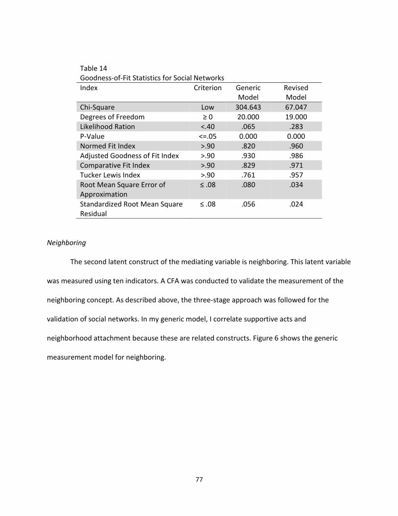
77
Table 14 Goodness-of-Fit Statistics for Social Networks Index Criterion Generic
Model Revised Model
Chi-Square Low 304.643 67.047 Degrees of Freedom ≥ 0 20.000 19.000 Likelihood Ration <.40 .065 .283 P-Value <=.05 0.000 0.000 Normed Fit Index >.90 .820 .960 Adjusted Goodness of Fit Index >.90 .930 .986 Comparative Fit Index >.90 .829 .971 Tucker Lewis Index >.90 .761 .957 Root Mean Square Error of Approximation
≤ .08 .080 .034
Standardized Root Mean Square Residual
≤ .08 .056 .024
Neighboring
The second latent construct of the mediating variable is neighboring. This latent variable
was measured using ten indicators. A CFA was conducted to validate the measurement of the
neighboring concept. As described above, the three-stage approach was followed for the
validation of social networks. In my generic model, I correlate supportive acts and
neighborhood attachment because these are related constructs. Figure 6 shows the generic
measurement model for neighboring.

78
Figure 6 Generic Measurement Model for Neighboring
Parameter estimates of the generic measurement model showed that all the
relationships were statistically significant. Factor loadings were checked to determine the
correlations between the latent construct of neighboring and its indicators. Factor loadings
ranged from .380 to .686.
The following step was an assessment of overall fit. Although the fit statistics were
within an acceptable range (see Table 16), there are concerns with discriminant validity for the
two neighboring constructs (supportive acts and neighborhood attachment).25 To assess
discriminant validity, I “compare the variance-extracted percentages for any two constructs
with the square of the correlation estimate between these two constructs. The variance-
extracted estimates should be greater than the squared correlation estimate. The logic is based 25 Construct reliability and validity are discussed in the next section. However, I am discussing discriminant validity for these two neighboring constructs in this section, because it is my rationale for change neighboring from two factors to one factor.

79
on the idea that the latent construct should explain its measures better than it explains another
construct” (Hair, Black, Babin, and Anderson, 2009; 802). For these two neighboring constructs,
the squared correlation estimate (.60) is greater than the Variance Extracted (VE) estimates
(supportive acts= .375 and attachment= .305). This means that these two constructs are not
unique, i.e., each construct captures phenomena that the other construct also measures.
Moving forward without addressing the discriminant validity concern can pose problems with
my full measurement model.
The next step is to compare the results (i.e., parameter estimates and fit statistics) from
a one and two factors neighboring construct. I dropped one indicator due to a low factor
loading (factor loading for miss neighborhood if you moved was .380). I put the remaining nine
items into one factor. The parameter estimates and fit statistics are acceptable. However,
modification indices suggest that I correlate the error terms for first name and stranger on
block. Therefore, I reran the CFA.
Table 15 shows the parameter estimates for the generic and revised measurement
models for neighboring. Figure 7 shows the revised model for the one factor neighboring
construct, which includes nine indicators. Although theoretically both supportive acts and
attachment are represented in the one factor neighboring construct, they are empirically
indistinguishable in this data. Reliability and validity for the one factor neighboring construct is
discussed on the next section.

80
Table 15 Parameter estimates for Neighboring
Generic Model
Revised Model
Indicator Std. Path
Std. Error
Z-value
p-value
Indicator Std. Path
Std. Error
Z-value p-value
Supportive Acts Asked personal question
.611
.015
28.44
0.00
Asked personal question
.588
.015
27.47
0.00
Borrow tools .668 .015 31.72 0.00 Borrow tools .652 .015 31.16 0.00 Lunch or dinner .652 .014 30.88 0.00 Lunch or
dinner .634 .014 30.06 0.00
Help with problem
.662 .013 31.37 0.00 Help with problem
.660 .013 31.62 0.00
Talk crime .442 .020 19.57 0.00 Talk crime .451 .020 20.19 0.00 Neighborhood attachment Said hello
.572
.010
25.56
0.00
Said hello
.532
.010
24.36
0.00
Stranger on block
.525
.011
23.14
0.00
Stranger on block
.378 .011 16.47 0.00
First name .686 .016 31.54 0.00 First name .577 .015 26.79 0.00 Neighbor watch my home
.555 .010 24.69 0.00 Neighbor watch my home
.503 .010 22.85 0.00
Likely miss neighborhood
.380 .020 16.24 0.00 First name <--> Stranger on block
.292 .006 11.94 0.00

81
Table 16 Goodness-of-Fit Statistics for Neighboring Index Criterion Generic Model Revised
Model Chi-Square Low 238.13 231.59 Degrees of Freedom ≥ 0 34.00 26.00 Likelihood Ration <.40 .076 .112 P-Value <=.05 0.000 0.000 Normed Fit Index >.90 .950 .948 Adjusted Goodness of Fit Index >.90 .966 .956 Comparative Fit Index >.90 .957 .954 Tucker Lewis Index >.90 .943 .936 Root Mean Square Error of Approximation
≤ .08 .052 .060
Standardized Root Mean Square Residual
≤ .08 .034 .038
Figure 7 Revised Measurement Model for Neighboring

82
Collective Efficacy
The third latent construct of the mediating variable is collective efficacy. Seven
indicators measured this latent variable. I conducted a CFA to validate the measurement of the
collective efficacy concept. As described above, I followed the three-stage approach for the
validation of collective efficacy. Figure 8 shows the generic measurement model for collective
efficacy.
Parameter estimates of the measurement model showed that all the relationships were
statistically significant. Factor loadings were checked to determine the correlations between
the latent construct of neighboring and its indicators. All of the indicators were above the .40
loading.
Figure 8 Generic Measurement Model for Collective Efficacy

83
The following step was an assessment of overall fit. The majority of the fit statistics were
within an acceptable range; however, the modification indices suggest that I correlate the error
terms between two variables. Figure 9 shows the revised model for the collective efficacy
construct, which includes seven indicators. One pair of error terms (People Trust and People
Help) was correlated. All of the items loaded between .49 and .71 and all regression coefficients
were statistically significant.
Figure 9 Revised Measurement Model for Collective Efficacy
Table 17 shows the parameter estimates for generic and revised measurement models
of neighboring. The goodness-of-fit statistics for the generic and revised measurement models

84
are shown in Table 18. There is a considerable decrease in the chi-square value. The difference
between the generic and revised models is 237.44, which shows an important improvement in
the revised model for collective efficacy. All other goodness-of-fit statistics are within the
acceptable range.
Table 17 Parameter Estimates for Collective Efficacy
Generic Model
Revised Model
Indicator Std. Path
Std. Error
Z-value
p-value Indicator Std. Path
Std. Error
Z-value p-value
Intervene if skipping school
.670 .019 32.12 0.00 Intervene if skipping school
.712 .019 34.24 0.00
Intervene if disrespect adult
.551 .018 25.34 0.00 Intervene if disrespect adult
.580 .018 26.70 0.00
Intervene if kids fighting
.594 .017 27.73 0.00 Intervene if kids fighting
.618 .017 28.81 0.00
Intervene if spraying graffiti
.590 .016 27.51 0.00 Intervene if spraying graffiti
.603 .016 27.95 0.00
People trustworthy
.574 .014 26.59 0.00 People trustworthy
.491 .014 21.84 0.00
People help neighbors
.630 .012 29.80 0.00 People help neighbors
.557 .013 25.331 0.00
Adults know kids
.636 .017 30.15 0.00 Adults know kids
.608 .017 28.23 0.00
People trustworthy <--> People help neighbors
.359 .007 13.91 0.00

85
Table 18 Goodness-of-Fit for Collective Efficacy Index Criterion Generic Model Revised Model Chi-Square Low 467.223 229.783 Degrees of Freedom ≥ 0 14 13 P-Value <=.05 0.00 0.00 Likelihood Ration <.40 .0299 .056 Normed Fit Index >.90 .884 .943 Adjusted Goodness of Fit Index >.90 .867 .937 Comparative Fit Index >.90 .887 .946 Tucker Lewis Index >.90 .830 .913 Root Mean Square Error of Approximation
≤ .08 .121 .087
Standardized Root Mean Square Residual
≤ .08 .059 .045
Crime Victimization
The fourth latent construct of the endogenous variable is crime victimization. This latent
variable was measured using seven indicators. I conducted a CFA to validate the crime
victimization construct. As previously described, I followed a three-stage approach to validate
this construct. Figure 10 shows the generic measurement model for crime victimization.

86
Figure 10 Generic Measurement Model for Crime Victimization
Parameter estimates of the generic measurement model show that all the relationships
are statistically significant. Factor loadings for four of the seven indicators were below .40,
approaching the critical value. However, only one factor loading was below .30, the minimum
accepted value. The indicators with factor loads below .40 are: (1) something taken by force
(.223), (2) physical attack (.306), (3) stolen car (.361), and (4) verbal threat (.369).
The following step was an assessment of overall fit. Overall, the evaluation of the crime
victimization construct showed that the model fit was not satisfactory (see Table 19). For
example, the chi-square seems high at 694.78. In order to obtain a better fit, the modification
indices suggest that I correlate the error terms between two sets of variables (damage to
property and home broken into, and verbal threat and physical threat).
Although the generic measurement model for crime victimization needs modification,
modifying the generic model based on low factor loadings and goodness-of-fit statistics does
not produce a single best-revised model. I revised the model over 9 times (analysis not shown

87
here) to try to find a better fitting model. For example, in reference to the generic model
above, when I drop something stolen by force and correlate the two sets of variables, the
goodness-of-fit statistics improve. However, multiple indicators now have factor loadings below
.30.
To revise the model, I have three basic choices. First, I keep the one-factor model for
crime victimization. This model would keep all seven indicators. However, one indicator will
have a factor loading below .30. Second, I could have a two-factor model for crime victimization
(personal and property crime victimization). However, a two-factor model is not a huge
improvement over a one-factor model. For example, additional indicators would be removed
due to low factor loadings (below. 30). Third, I could have a one-factor model for property
crime victimization or personal crime victimization. Based on theoretical interests and empirical
considerations, I decide to pick my first choice and keep a one-factor model for crime
victimization.
Figure 11 shows the revised for crime victimization. Based on modification indices, I
correlated the error terms for three sets of indicators. Note that three indicators have factor
loadings below .30. All regression coefficients were significant at the .05 level. Table 19 shows
the parameter estimates for the generic and revised model for crime victimization.

88
Figure 11 Revised Measurement Model for Crime Victimization
Table 19 Parameter Estimates for Crime Victimization
Generic Model
Revised Model
Indicator Std. Path
Std. Error
Z-value
p-value
Indicator Std. Path
Std. Error
Z-value
p-value
Property damaged
.503 .046 18.90 0.00 Property damaged
.358 .052 11.76 0.00
Property stolen (e.g., bicycle)
.485
.063
18.26
0.00
Property stolen (e.g., bicycle)
.614
.077
18.87
0.00 Car stolen or broken into
.361
.059
13.58
0.00
Car stolen or broken into
.422
.063
14.75
0.00
Home broken into
.577
.046
21.41
0.00
Home broken into
.489
.052
16.10
0.00
(table continues)

89
Table 19 Parameter Estimates for Crime Victimization (continued)
Generic Model
Revised Model
Indicator Std. Path
Std. Error
Z-value
p-value
Indicator Std. Path
Std. Error
Z-value
p-value
Verbally threatened
.369
.329
13.88
0.00
Verbally threatened
.290
.348
10.29
0.00
Physically attacked
.306
.156
11.45
0.00
Physically attacked
.151
.166
5.29
0.00
Something stolen by force (e.g., mugging)
.223
.034
8.29
0.00
Something stolen by force (e.g., mugging)
.161
.036
5.71
0.00 Physically
attacked <--> Verbally threatened
.459
1.64
19.05
0.00 Home broken
into <--> Property damaged
.264
0.07
8.91
0.00 Physically
attacked <--> Something stolen by force
.190
0.14
9.73
0.00
As seen in Table 20, the goodness-of-fit statistics signified improved. There is a
considerable decrease in chi-square value. The chi-square difference between the generic and
final models is 666.618, which is an improvement in the final model. The goodness-of-fit
statistics are improved and within acceptable range.
Table 20 Goodness-of-Fit Statistics for Crime Victimization Index Criterion Generic Model Revised Model Chi-Square Low 694.78 28.162 Degrees of Freedom ≥ 0 14.0 11 P-Value <=.05 0.00 0.00 Likelihood Ration <.40 .020 .390 (table continues)

90
Table 20 Goodness-of-Fit Statistics for Crime Victimization (continued) Index Criterion Generic Model Revised Model
Normed Fit Index >.90 .585 .983 Adjusted Goodness of Fit Index >.90 .839 .991 Comparative Fit Index >.90 .588 .990 Tucker Lewis Index >.90 .383 .980 Root Mean Square Error of Approximation
≤ .08 .148 .027
Standardized Root Mean Square Residual
≤ .08 .090 .020
Full Measurement Model
After conducting the CFAs on the individual constructs, I put all of the constructs into
one model to confirm the statistical fit with the data. The measurement model showed
adequate fit (χ² (419) = 1665. 835, RMSEA = .037, NNFI = .899, CFI = .909, SRMR = .039).
I examined reliability and validity for each construct in the full measurement model (see
Table 21). To assess the reliabilities of the measures used in my analysis, I examined the
individual composite reliabilities suggested by Fornell and Larker (1981). Composite reliabilities
were adequate for all of the constructs, ranging from .886 to .995. Therefore, there is good
construct reliability for all constructs. Additionally, I examined AVE for each construct, as
suggested by Fornell and Larker. All constructs have AVEs above the recommended critical
value of .500, ranging from .570 to .958. This means that the variance due to measurement
error is smaller than the variance captured by each construct. Note that crime victimization has
an AVE of .570, just above the recommended critical value.
The VE indicates some concern for two of the five constructs: non-neighborhood social
networks (VE=.17) and crime victimization (VE=.15). These values mean that non-neighborhood

91
social networks and crime victimization have more variability and error compared to the other
constructs in the full model. For non-neighborhood social networks, the variability is due to the
large spread in responses among all four indicators. For crime victimization, the variability is
also due to the large spread in responses. In particular, there is large spread in responses for
two indicators (physically attacked and verbally threatened). The implication of a low VE means
that I am not completing measuring the non-neighborhood social networks concept or the
crime victimization concept. I am not claiming that either construct is measure most or all types
of social networks or crime victimization.
I also examined discriminant validity as suggested by Fornell and Larker (1981). To
assess discriminant validity, I compare HSV to VE values. For three of the five constructs (non-
neighborhood social constructs, collective efficacy, and crime victimization), HSV is smaller than
the VE, which indicates adequate discriminant validity for these constructs. However, HSV is
greater than VE for neighboring and neighborhood social networks, which indicates a lack of
discriminant validity. That is, these two constructs are more closely related compared to all the
other constructs in the model (e.g., they are separate but related constructs). Said differently,
neighboring and neighborhood social networks have more shared variance than distinct
variance in relation to the other constructs. This issue (lack of discriminant validity) is not
unexpected based on theory (as discussed in Chapter 2).
In analysis not presented here, I put all neighboring and neighborhood social network
indicators into a factor analysis and results show that they are separate constructs. The
correlations between these two latent constructs are strong (.643) but not too strong to worry
about multicollinearity. The path coefficients are small (under .50). The goodness-of-fit

92
statistics are acceptable for both constructs. I accept some lack of discriminant validity for these
two construct neighboring and neighborhood social networks based on theory. To address this
issue, I correlate neighboring and neighborhood social networks. See Figure 12. Correlations
among latent constructs are presented in Table 22.
Table 21 Parameters of the measurement model, standardized path coefficient, z values, composite reliability, average variance extracted, variance extracted, and highest shared variance
Neighborhood Social Networks
Non-Neighborhood
Social Networks Neighboring Collective Efficacy
Crime Victimization
Path z Path z Path z Path z Path z Block Party .538 23.00 - - - - - - - - Other block party .733 31.45 - -
- -
- -
- -
Neighborhood associations .572 24.58 - -
- -
- -
- -
Church orgs - - .347 12.67 - - - - - - Recreational orgs - -
.429 15.59 - -
- -
- -
Service orgs .505 18.17 Race/ethnic orgs - -
.334 12.13 - -
- -
- -
Other orgs - - .457 16.58 - - - - - - Asked a personal question - -
- -
.570 26.83 - -
- -
Borrow tools - - - - .624 30.0 - - - - Lunch or dinner - - - - .623 29.98 - - - - Help with problem - -
- -
.647 31.44 - -
- -
Talk crime - - - - .459 20.90 - - - - Said hello - - - - .540 25.24 - - - - Stranger on block - -
- -
.416 18.60 - -
- -
First name - - - - .618 29.59 - - - - (table continues)

93
Table 21 Parameters of the measurement model, standardized path coefficient, z values, composite reliability, average variance extracted, variance extracted, and highest shared variance (continued)
Neighborhood Social Networks
Non-Neighborhood
Social Networks Neighboring Collective Efficacy
Crime Victimization
Path z Path z Path z Path z Path z Neighbor watch my home - -
- -
.515 23.83
- -
Intervene if skipping school - -
- -
- -
.686 33.18 - -
Intervene if disrespect adult - -
- -
- -
.571 26.48 - -
Intervene if kids fighting - -
- -
- -
.602 28.33 - -
Intervene if spraying graffiti - - - -
- -
.587 27.34
- -
People trustworthy - - - -
- -
.510 22.99
- -
People help neighbors - - - -
- -
.596 27.75
- -
Adults know kids - -
- - - -
.638 30.26
- -
Property stolen (e.g., bicycle) - -
- -
- -
- - .595 19.40
Car stolen .427 15.14 Property damaged - -
- -
- -
- - .369 12.31
Home broken into - -
- -
- -
- - .496 16.76
Verbally threatened - -
- - - -
- - .295 10.55
Physically attached - -
- - - -
- - .160 5.63
Something taken by force - -
- - - -
- - .170 6.08
Composite Reliability .985 .977 .995 .993 .886 AVE .958 .958 .898 .956 .570 HSV .313 .381 .176 .358 .150 Measurement Model χ² (419) = 1665. 835; RMSEA = .037; NNFI = .899; CFI = .909; SRMR = .039. AVE = average variance explained; VE = variance extracted; HSV = highest shared variance.

94
Figure 12 Measurement Model For All Constructs with Parameter Estimates and Error Terms

95
Based on the results from the measurement models, my empirical model to be tested
using structural equation modeling is presented in Figure 13. This figure includes social
structural variables and arrows denote the hypothesized relationships as specified on pages 44-
47 in Chapter 3.
Table 22 Correlations Between Latent Constructs Variables Neighborhood
Social Networks
Non-Neighborhood Social Networks
Neighboring Collective Efficacy
Crime Victimization
Neighborhood Social Networks
1.00
Non-Neighborhood Social Networks
.515
1.00
Neighboring .643 .460 1.00
Collective Efficacy .422 .247 .543 1.00
Crime Victimization
.123 .182 .202 -0.033 1.00

96
Figure 13 My Empirical Model

97
Structural Equation Modeling
Based on the results from the CFAs, I developed a generic model that included the five
latent constructs (neighborhood social networks, non-neighborhood social networks,
neighboring, collective efficacy, and crime victimization) and six exogenous measures (racially
homogeneous neighborhood, resident tenure, annual household income, family disrupted,
male, and non-white race). The generic structural equation model is presented in Figure 14.
As in the CFA, the three-stage method was used for the SEM analysis. First, the generic
structural equation model was developed. The statistical significant levels based on the critical
ratios and factor loadings were checked. According to the parameter estimates in Table 22,
seven hypothesized pathways between were insignificant. Two of the seven insignificant
pathways were between latent variables. These insignificant paths were non-neighborhood
social networks and collective efficacy (r=.06, p-value=.075) and neighborhood social networks
and crime victimization (r=-.045, p-value=.431). The remaining insignificant pathways were
between social structural variables and latent variables. These include: (1) family disrupted and
collective efficacy (r=.028, p-value=.171); (2) family disrupted and neighborhood social
networks (r=.005, p-value =.833); (3) family disrupted and non-neighborhood social networks
was insignificant (r=.016, p-value=.594); (4) racially homogeneous neighborhood and
neighborhood social networks (r=.021, p-value=.417); and (5) non-white ethnicity and crime
victimization (r=-.039, p-value=.171). These regression paths were eliminated from the model.
Based on the results from the modification indices, I also correlated neighboring and non-
neighborhood social networks. The SEM analysis was run again. The revised model is presented
in Figure 15. All of the pathways were statistically significant. Therefore, all of the items of the

98
measurement models and regression paths remained in the structural equation model. An
assessment of overall fit followed. Table 22 shows the parameter estimates for the generic and
revised structural equation model of the study.
The goodness-of-fit statistics are fair to the data (see Table 23). The chi-square was
reduced by 173.57. The likelihood ratio (.227), adjusted goodness of fit index (.922), root mean
square error of approximation (.039), and standardized root mean square residual (.041) were
within acceptable range. Some of the statistics are not within acceptable ranges. For example,
the normed fit index value (0.832), comparative fit index (.865) and the Tucker Lewis Index
(.852) are just below the critical value of .90. Figure 14 shows the revised structural equation
model. All critical ratios were significant at the .05 level for the revised model.
The revised structural equation model results show that neighboring has the highest
regression weight on collective efficacy (.435), followed by income on neighboring (.272),
collective efficacy on crime victimization (-.236) and neighboring on crime victimization (.257).
Hypotheses testing based on the results of the SEM is discussed in the following section.
Additional analyses (not shown here) were conducted to improve the model fit of the
revised SEM (figure 15). However, these analyses (i.e., reducing the items per construct,
removing latent constructs) were unsuccessful. The goodness-of-fit statistics only slightly
improved (statistics were still under .90). One reason why the model statistics, in particular the
Tucker Lewis Index and the comparative fit index, are not meeting the critical values of .90 may
be due to the dichotomous variables in my model (Kenny, 2014.). These model statistics
depend on the average size of the correlations in the data and dichotomous variables have zero
correlations with each other. In these events, the root mean square error of approximation for

99
the null model should be no smaller than 0.158, otherwise, an incremental measure of fit may
not be that informative (Kenny, 2014).
With the current fit statistics for my revised structural equation model, it is not
necessary to artificially drop significant constructs. As is, the current revised structural equation
model (figure 15) lends support for my thesis, although I cannot be completely confident.
Additional testing is necessary, ideally with data meant to test my revised structural equation
model.

100
Figure 14 Generic Structural Equation Model

101
Figure 15 Revised Structural Equation Model

102
Table 23 Parameter Estimates for Generic and Revised SEM
Generic Model Revised Model Indicator Std.
Path Std. Error
Z-value P-value
Indicator Std. Path
Std. Error
Z-value P-value
Neighboring<-- Racial Homogeneity Neighborhood
0.071 0.049 3.084 0.002 Neighboring<-- Racial Homogeneity Neighborhood
0.061 0.044 2.962 0.003
Neighboring<--Resident Tenure
0.165 0.002 7.252 0.000 Neighboring<--Resident Tenure
0.166 0.002 7.309 0.000
Neighboring<-- Income
0.271 0.008 11.524 0.000 Neighboring<-- Income
0.268 0.008 11.45 0.000
Neighboring<-- Non-White
-0.07 0.055 -3.359 0.001 Neighboring<-- Non-White
-0.092 0.054 -4.541 0.000
Neighboring<-- Male
-0.089 0.044 -4.329 0.000 Neighboring<-- Male
-0.078 0.043 -3.935 0.000
Collective Efficacy <--Racial Homogeneity Neighborhood
0.241 0.054 11.134 0.000
Collective Efficacy <--Racial Homogeneity Neighborhood
0.236 0.054
11.052
0.000
Collective Efficacy <--Neighborhood Social Networks
0.108 0.05 2.573 0.010
Collective Efficacy <--Neighborhood Social Networks
0.134 0.045 3.570 0.000
Collective Efficacy <--Non-Neighborhood Social Networks
0.06 0.041 1.781 0.075
Collective Efficacy <--Neighboring
0.438 0.044 11.619 0.000 Collective Efficacy <--Neighboring
0.435
0.044 11.505 0.000
(table continues)

103
Table 23 Parameter Estimates for Generic and Revised SEM (continued)
Generic Model Revised Model Indicator Std.
Path Std. Error
Z-value
P-value
Indicator Std. Path
Std. Error
Z-value
P-value
Collective Efficacy <--Family Disrupted
0.028 0.116 1.37 0.171
Neighborhood Social Networks <--Racial Homogeneity Neighborhood
0.021 0.054 0.812 0.417
Neighborhood Social Networks <--Resident Tenure
0.222 0.002 8.417 0.000
Neighborhood Social Networks <--Resident Tenure
0.219 0.002 8.478 0.000
Neighborhood Social Networks <--Income
0.185 0.009 7.003 0.000 Neighborhood Social Networks <--Income
0.184 0.009 7.154 0.000
Neighborhood Social Networks <--Family Disrupted
0.005 0.111 0.211 0.833
Non-neighborhood Social Networks <--Racial Homogeneity Neighborhood
-0.081 0.061 -2.729 0.006
Non-neighborhood Social Networks <--Racial Homogeneity Neighborhood
-0.083 0.058 -2.929 0.003
(table continues)

104
Table 23 Parameter Estimates for Generic and Revised SEM (continued)
Generic Model Revised Model Indicator Std.
Path Std. Error
Z-value P-value
Indicator Std. Path
Std. Error
Z-value
P-value
Non-neighborhood Social Networks <--Resident Tenure
0.177 0.002 5.959 0.000
Non-neighborhood Social Networks <--Resident Tenure
0.167 0.002 5.623 0.000
Non-neighborhood Social Networks <--Income
0.143 0.01 4.783 0.000
Non-neighborhood Social Networks <--Income
0.144
0.01 4.846 0.000
Non-neighborhood Social Networks <--Family Disrupted
0.016
0.134
0.532
0.594
Crime Victimization<--Neighborhood Social Networks
-0.045 0.059 -0.787 0.431
Crime Victimization<--Non-neighborhood Social Networks
0.146 0.048 3.125 0.002
Crime Victimization<--Non-neighborhood Social Networks
0.108 0.048 2.333 0.020
Crime Victimization<--Collective Efficacy
-0.238 0.035 -5.714 0.000 Crime Victimization<--Collective Efficacy
-0.236 0.035 -5.674 0.000
Crime Victimization<--Neighboring
0.299 0.056 5.272 0.000 Crime Victimization<--Neighboring
0.257 0.049 5.181 0.000
(table continues)

105
Table 24 Goodness-of-Fit Statistics for Generic and Revised SEM Index Criterion Generic Model Revised Model Chi-Square Low 2780.784 2607.214
Degrees of Freedom ≥ 0 587 593 P-value <=.05 0.000 0.000 Likelihood Ration <.40 .211 .227 Normed Fit Index >.90 0.821 0.832 Adjusted Goodness of Fit Index >.90 0.917 .922 Comparative Fit Index >.90 0.853 0.865 Tucker Lewis Index >.90 0.837 0.852 Root Mean Square Error of Approximation
≤ .08 0.041 0.039
Standardized Root Mean Square Residual
≤ .08 0.049 0.041
Table 23 Parameter Estimates for Generic and Revised SEM (continued)
Generic Model Revised Model Indicator Std.
Path Std. Error
Z-value
P-value
Indicator Std. Path
Std. Error
Z-value
P-value
Crime Victimization<--Income
0.106 0.011 3.513 0.000 Crime Victimization<--Income
0.119 0.011 4.008 0.000
Crime Victimization<-- Non-White
-0.039 0.075
-1.368 0.171
Crime Victimization<--Male
0.104 0.061 3.641 0.000 Crime Victimization<--Male
0.099
0.06 3.500 0.000
Crime Victimization<--Family Disrupted
0.093 0.136 3.278 0.001 Crime Victimization<--Family Disrupted
0.090
0.134 3.203 0.001

106
Summary of Hypotheses Tested
The following hypotheses were proposed in Chapter 3:
H1: Collective efficacy has a direct negative effect on crime victimization.
This hypothesis was supported. I found that collective efficacy has a direct negative
effect on crime victimization (β = -.236, p ≤ 0.00).
H2: Social networks have a direct negative effect on crime victimization. Social networks also
have an indirect negative effect on crime victimization through increasing collective efficacy.
These hypotheses were partly supported. Non-neighborhood social networks have a
weak direct positive effect on crime victimization (β = .108, p ≤ 0.00). Examples of non-
neighborhood social networks include participation in church activities and recreational
organizations activities, such as sports, book club, or card playing. Neighborhood social
networks did not have a statistically significant direct relationship with crime victimization.
However, neighborhood social networks have an indirect effect on crime victimization through
increasing collective efficacy (β = .134, p ≤ 0.00). This is consistent with my hypothesis. Non-
neighborhood social networks did not have a statistically significant indirect effect on crime
victimization.
H3: Neighboring has a direct negative effect on crime victimization and an indirect negative
effect on crime victimization through increasing collective efficacy.

107
These hypotheses were partly supported. Neighboring had a weak direct positive effect
on crime victimization (β = .257, p ≤ 0.00). However, neighboring also had an indirect negative
effect on crime victimization through increasing collective efficacy (β = .435, p ≤ 0.00), as
hypothesized. The total indirect effect for neighboring and crime victimization is -0.102, which
is smaller than the direct effect of .257, which indicates an overall very weak positive effect
between neighboring and crime victimization.
H4: Residents from homogenous neighborhoods are more likely to neighbor, engage in social
networks, and have collective efficacy and therefore are less likely to be crime victims
compared to residents from racial/ethnic heterogeneous neighborhoods.
These hypotheses were partly supported. As hypothesized, residents in racial/ethnic
homogeneous neighborhoods were more likely to neighbor compared to those in racial/ethnic
heterogeneous neighborhoods (β = .061, p ≤ 0.00). Residents in racial/ethnic homogeneous
neighborhoods were also more likely to increase collective efficacy (β = .236, p ≤ 0.00). On the
other hand, residents from racial/ethnic homogeneous neighborhoods were less likely to
engage in non-neighborhood social networks (β = -.083, p ≤ 0.00) compared to those in
racial/ethnic heterogeneous neighborhoods and there was no statistically significant
relationship between residents in racial/ethnic homogeneous neighborhoods and
neighborhood social networks.
H5: Resident tenure has an indirect negative effect on crime victimization through increasing
social networks and neighboring, and through increasing collective efficacy.

108
These hypotheses were partly supported. First, resident tenure had an indirect negative
effect on crime victimization through increasing neighborhood social networks (β = .219, p ≤
0.00) and then increasing collective efficacy (β = .134, p ≤ 0.00), as discussed in hypothesis 2.
Resident tenure also had an indirect negative effect on crime victimization through increasing
neighboring (β = .166, p ≤ 0.00) and then through increasing collective efficacy (β = .435, p ≤
0.00). However, resident tenure did not have an indirect negative effect on crime victimization
through increasing non-neighborhood social networks and then through increasing collective
efficacy. Although resident tenure increased non-neighborhood social networks (β = .167, p ≤
0.00), non-neighborhood social networks did not have a statistically significant relationship with
collective efficacy.
H6: Household income has a direct negative effect on crime victimization. Household income
also has an indirect negative effect on crime victimization through increasing social networks
and neighboring, and then through increasing collective efficacy.
These hypotheses were partly supported. Inconsistent with my hypothesis, household
income had a weak direct positive effect on crime victimization (β = .119, p ≤ 0.00). Consistent
with my hypotheses, household income had an indirect negative effect on crime victimization
through increasing neighborhood social networks (β = .184, p ≤ 0.00), and then through
increasing collective efficacy (β = .134, p ≤ 0.00). Household income also had an indirect
negative effect on crime victimization through increasing neighboring (β = .268, p ≤ 0.00), and
then through increasing collective efficacy (β = .435, p ≤ 0.00). However, household income did
not have an indirect negative effect on crime victimization through increasing non-

109
neighborhood social networks and then through increasing collective efficacy. Although
household income increased non-neighborhood social networks (β = .144, p ≤ 0.00), non-
neighborhood social networks did not have a statistically significant relationship with collective
efficacy.
H7: Residents from disrupted families are more likely to be crime victims compare to intact
families, and they are more likely to be crime victims because these residents engage in social
networks less and have less collective efficacy.
These hypotheses were partly supported. Residents from disrupted families are more
likely to be crime victims compared to those from intact families (β = .090, p ≤ 0.00). There
were no statistically significant relationships between family disruption and neighborhood
social networks, non-neighborhood social networks, or collective efficacy.
H8: Males are more likely to be crime victims compared to females. I hypothesize that men are
more likely to become crime victims because they neighbor less compared to women.
These hypotheses were partly supported. Males were more likely to be crime victims
compared to females (β = .099, p ≤ 0.00). This was a weak relationship. Men neighbor less
compared to women (β = -.078, p ≤ 0.00); however, neighboring has a dual nature with crime
victimization (neighboring directly increases crime and indirectly decreases crime through
collective efficacy).

110
H9: Non-whites are more likely to be crime victims compared to whites, and they are more
likely to be crime victims because they are less likely to neighbor.
These hypotheses were partly supported. There was no statistically significant direct
relationship between non-whites and crime victimization. Non-whites were less likely to
neighbor compared to whites (β = -.092, p ≤ 0.00); however, neighboring has a dual nature with
crime victimization (neighboring directly increases crime and indirectly decreases crime through
collective efficacy).

111
Chapter 6
DISCUSSION AND CONCLUSION
This chapter summarizes and discusses the findings in this study. This chapter also
presents the implications of the findings. Finally, this chapter identifies the limitations of this
study and presents recommendations for future research.
Summary of Findings and Discussion
There is a long-standing debate about the sources of neighborhood influence on crime
victimization. To address this debate, the systemic model, which is grounded in social
disorganization theory, argues that social ties are a prerequisite for effective informal social
control, which in turn reduces crime victimization. However, many studies do not test the full
systemic model (e.g., due to problems with conceptualization and measurement). Furthermore,
I argue that the systemic model is an oversimplification of the relationship between
neighborhoods and crime victimization.
I developed an alternative to the systemic model as a way to address these major
outstanding analytical issues. Although my alternative model is similar to the [full] systemic
model, it incorporates neighboring, which clarifies conceptual and measurement confusion in
the literature. In my alternative model, I make a conceptual distinction between neighboring
and social networks, and develop measures of each concept that are clearly distinguishable
from each other. Neighboring represents social support and attachment whereas social
networks represent organizational participation, which reflect linkages or pathways between a
community and its institutions. While neighboring and social networks generate social capital,

112
collective efficacy is the action component in my model. Unlike the systemic model, my
alternative model does not assume that friendship is required for neighboring and social
networks. The purpose of this study is to develop and test my alternative model. I test new
hypotheses not originally included in the systemic model. Although different from the systemic
model, my results have implications for clarifying social disorganization theory.
My Alternative Model
Overall, I found partial support for my hypothesized [alternative] model (see figure 3).
The results supports my argument that the systemic model is too simplistic, but the
relationships among the variables are not exactly as I hypothesized. Three hypothesized effects
among the latent variables were in the expected direction. Collective efficacy directly reduces
crime victimization. Neighborhood social networks and neighboring both have an indirect
negative effect on crime victimization through collective efficacy.
The remaining relationships were not expected. Neighborhood social networks did not
have a statistically significant direct relationship with crime victimization as hypothesized.
Additionally, I found that both non-neighborhood social networks and neighboring directly
increase crime victimization, contrary to what I hypothesized. Interestingly, I also found that
neighborhood social networks and neighboring positively effect collective efficacy, which in
turn reduces crime victimization.
Among the hypothesized effects between the social structural variables and the latent
variables, the majority of my hypotheses were supported. Disrupted families and males both
have a direct positive effect on crime victimization, consistent with my hypotheses. Non-whites

113
are less likely to neighbor compared to whites, which is also consistent with my hypothesis.
Finally, racial/ethnic homogeneous neighborhoods were associated with higher collective
efficacy, neighboring, and one type of social networks (non-neighborhood social networks)
compared to racial/ethnic heterogeneous neighborhoods. However, there were no statistically
significant relationships between racial/ethnic homogeneous neighborhoods and neighborhood
social networks or between non-whites and crime victimization, as hypothesized. Higher
household income has a direct positive effect on crime victimization, which is opposite than
predicted.
Another major contribution of this study is clarifying measurement inconsistencies. I
found that neighboring and social networks are empirically distinct concepts, as theorized.
However neighboring does not contain sub-dimensions as hypothesized. Theoretically,
neighboring measures supportive acts and neighborhood attachment. Furthermore, I did not
expect two separate social network constructs (neighborhood and non-neighborhood social
networks). My findings should help researchers when deciding which indicators to use in future
research; however, more testing is needed.
Social Disorganization Theory
The results from this study show modest support for the systemic model. In this study,
the only relationship consistent with the systemic model was between collective efficacy and
crime victimization. However, my other findings provide an important advancement for the
systemic model. As I argued, my results show the systemic model is too simplistic. My findings
show that non-neighborhood social networks and neighboring had direct effects on crime

114
victimization. Both neighboring and non-neighborhood social networks increase crime
victimization. Neighboring also positively effects collective efficacy, which in turn reduces crime
victimization. Although inconsistent with social disorganization theory, some previous research
shows a dual nature for neighboring (neighboring is often measured as social networks) -
neighboring both increases collective efficacy and increases crime victimization (see Browning,
Feinberg, and Dietz, 2004; Bellair and Browning, 2010).
There are several interpretations for why neighboring (however operationalized) has a
dual nature. One interpretation is that while neighboring promotes cohesion and orientations
for collective efficacy, neighboring also generates social capital for offenders who may embed
themselves in local networks or communities, referred to as the negotiated coexistence model
by Browning, Feinberg, and Dietz (2004). Another interpretation is that weak neighboring
exerts minimal regulatory effects on crime victimization. Specifically, weak social contact may
facilitate trust and share values without also fostering mutual obligations for collective action.
Inconsistent with the systemic model, I also found that disrupted families did not have
an indirect relationship with crime victimization. Instead, there is only a direct relationship
between family disrupted and with crime victimization. Among the relationships that supported
the theory, resident tenure and (higher) household income were both associated with higher
rates of neighboring, neighborhood social networks, and non-neighborhood social networks.
Furthermore, racial/ethnic homogeneous neighborhoods were associated with higher collective
efficacy compared to racial/ethnic heterogeneous neighborhoods. The theory posits that
collective efficacy should be higher in racial/ethnic homogeneous neighborhoods.

115
Furthermore, my findings indicate that social networks contain two separate empirical
dimensions – neighborhood social networks and non-neighborhood social networks – not one
dimension as previously predicted. These two social network constructs impact crime
victimization differently. Neighboring and social networks are also distinct empirical
phenomena, albeit they are related. These findings help to clarify the relationships between
neighboring, social networks, and collective efficacy on crime victimization.
Implications of the Findings
The findings from this study have important implications for advancing research on the
theory of the systemic model. As theorized, this study shows that the systemic model is more
complex than previously predicted and it offers insight into the complex relationships among
neighboring, neighborhood and non-neighborhood social networks, collective efficacy, and
crime victimization. For example, neighboring and social networks are not only different
constructs, but they effect crime victimization in very different ways. As previously discussed,
neighboring directly and indirectly effects crime victimization; it also has a dual nature with
crime victimization. Non-neighborhood social networks directly increase crime victimization,
whereas neighborhood social networks indirectly decrease crime victimization.
Of interest here are the relationships between neighboring and both types of social
networks on crime victimization. It is unclear why they effect crime victimization differently as
they are closely related constructs. Perhaps these relationships are task dependent. For
example, Wickes, Hipp, Sargeant, and Homel (2013) found collective efficacy for violence, child
centered control and political/civic matters were distinct constructs. Additionally, these authors

116
also found that neighborhood level cohesion only increases collective efficacy regarding
controlling children, and at the same time, social ties were positively related to cohesion as well
as all types of collective efficacy. Wickes, Hipp, Sargeant, and Homel (2013) point out that an
overlooked component of the theory is the task specific nature of collective efficacy - which
serves a more useful purpose than simply refining measurement. Their research may have
implications for my model, as the extent to which the task specific nature of not just collective
efficacy, but also neighboring and social networks is unknown. Future scholarship should
consider the task at hand and the degree to which the task requires collective action versus
individual action.
This study also includes social structural characteristics that are often missing from the
literature. I added two variables to my model that have implications for social disorganization
theory. First, I included gender. Gender is not traditionally included in social disorganization
research. However, research shows that crime victimization is generally higher for males than
females (Lauritsen and Heimer, 2008). For example, there are gender gaps between men and
women in robbery victimization, aggravated assault victimization, and simple assault
victimization. Furthermore, males are consistently found to be less active in neighboring than
women (Campbell and Lee, 1990; Kusenbach, 2006). This study found that males had a direct
positive relationship with crime victimization and were also less likely to neighbor compared
with females. To help clarify the relationship between gender and neighboring and given the
strong relationship between gender and crime victimization, I argue that gender should be
included as a variable in future research.

117
Second, I included race/ethnicity in my in model. Although previous research indicates
inconsistent racial difference in neighboring, some studies demonstrate that blacks are less
likely to engage in social neighboring compared to non-blacks (Nation, Fortney, and
Wandersman, 2010; Ignatow, Poulin, Hunter, and Comeau, 2013). My study found that whites
were less likely to neighbor compared with non-whites. To help clarify the relationship between
race/ethnicity and neighboring, I argue that race/ethnicity should be included in future
research.
Additional research will not only help the theory, but also policies and programs
targeted at neighborhood crime prevention, which is a perennial goal of government and other
community interventions (Chaskin, Brown, Venkatesh, and Vidal, 2001). If it is the efficacious
nature of a neighborhood rather than its support or social networks that constitute the social
mechanism for explaining between-neighborhood variations in crime victimization, then
policies that encourage neighboring, social ties, and organizational participation seem
misguided. On the other hand, there may be specific issues that require targeted interventions
or neighbor involvement, so identifying the factors or behaviors associated with increased
community regulation must be the next goal of researchers. Until we know more,
neighborhood interventions and revitalization efforts should focus directly on supporting
cohesion and attachment among residents, thereby generating collective efficacy and reducing
crime victimization. The influences for collective efficacy can differ by neighborhood context.
In summary, my findings provide insight into the complex relationships among
neighboring, neighborhood and non-neighborhood social networks, collective efficacy, and
crime victimization. Even with this insight, there is still a lack of theoretical clarity among these

118
variables. Although theories of neighborhood social disorganization have not fully explained
these relationships, my research points the direction for future research.
Limitations and Directions for Future Research
Several limitations exist with my study. First, my alternative model may have a temporal
order problem. Consistent with social disorganization theory, my model assumes crime
victimization is the outcome of neighboring, social networks, and/or collective efficacy.
However, it is possible that crime victimization happens first; that neighboring, social networks
and/or collective efficacy is the result of crime victimization. Second, my alternative model is
limited to a stereotypical concept of crime victimization (e.g., street crime victimization) within
neighborhoods. My alternative model does not address many other important types of crime
victimization, such corporate crime or white-collar crime. This limitation is common in all social
disorganization research. Third, conceptualization and operationalization of all concepts is
limited to the data available in the dataset. Not all variables were measured exactly as they
were in other studies (e.g., I measured household income rather than socio-economic status).
The findings and limitations of this study point to directions for future research. The
findings suggest that we need a theoretical elaboration of the processes between neighboring,
neighborhood and non-neighborhood social networks, collective efficacy, and crime
victimization. Future research would greatly benefit from a more detailed and subtle
understanding of the joint influence of social networks and neighboring on the control and
facilitation of crime victimization. Qualitative studies may play a key part in advancing our
understanding of the joint influence of social networks and neighboring; most studies are

119
quantitative. For example, Desmond’s (2012) qualitative work could serve as an analytical tool
for future research. As argued in this study, the binary between weak and strong social contact
(e.g., neighboring or social networks) may not be very useful in examining neighborhoods in
21st century America. In his qualitative study, Desmond shows that the function, not the
strength, of the social network is more important. Unfortunately, my data did not allow me to
test this hypothesis. However, future research could test whether Desmond’s conceptualization
of social networks sheds light into the dual nature of neighboring and social networks on crime
victimization.
As discussed in the previous section, future research should consider whether
neighboring, social networks, and collective efficacy are a task specific processes. In addition,
results from this study need to be tested with better data, data that is meant to specifically test
the relationships between the concepts in my empirical model, including the social structural
variables included in my study. This would also advance our understanding of the findings in
this study.
Continued efforts to collect data at the neighborhood and block level will allow future
research to test the negotiated coexistence model by Browning, Feinberg, and Dietz (2004).
Another possibility for future research is to specify the relationship between neighboring,
neighborhood social networks and collective efficacy for specific types of crime victimization.
Additional testing of measurement models for social networks and neighboring are welcomed,
even though the findings of my measurement models are promising. Lastly, future research
should test the systemic theory in different neighborhood contexts (e.g., neighborhoods in the
urban core, neighborhoods with gentrification, neighborhoods in the inner ring suburbs,

120
neighborhoods in new urban areas within cities, pedestrian neighborhoods, ethnic
neighborhoods, etc.).

121
APPENDIX
CORRELATION MATRICES FOR VARIABLES USED IN ANALYSIS

122
Table A.1 Correlation Matrix of Social Network (SN), Neighboring (Nghr), Collective Efficacy (CE) and Crime Victimization (CV) by Social Structural Variables, Seattle Adults, 2002-2003 Variables Race/Ethnic
Homogeneous Resident Tenure
Income Family Disrupted
Male Non-White
SN–block party .093** .179** .098** .023 -.028 -.081** SN–other block party .025 .097** .122** .021 -.024 -.071** SN–church .009 .189** -.015 .027 -.029 .064** SN–recreational orgs .005 -.025 .134** .004 -.030 .017 SN–service orgs -.046* .065** .056** -.027 .022 .019 SN–race/ethnic orgs -.032 .064** -.020 .015 -.045* .132** SN–neighborhood associations .042 .140** .083** -.020 -.011 -.071** SN–other orgs .001 .053* .070** .018 -.050* -.046* Nghr–first name .124** .252** .202** .035 -.065* -.113** Nghr–borrow tools .096** -.023 .179** -.005 -.041 -.104** Nghr–lunch or dinner .073** .056 .105** .009 -.058** -.100** Nghr–help with problem .048* .165** .108** .011 -.004 -.096** Nghr–asked personal questions .076** -.078** .152** .028 -.059** -.091** Nghr–said hello .102** .065** .165** .011 -.052* -.090** Nghr–stranger on block .096** .159** .138** .027 -.020 -.037 Nghr–talk crime -.001 .078** .066** .021 -.045* -.057** Nghr–likely miss neighborhood .159** .048* .116** ,014 -.091** -.044** Nghr–neighbor watch my home .120** .188** .249** .035 -.088** -.136** CE–intervene if skipping school .193** .167** .145** .046* -.051* -.061** CE–intervene if spraying graffiti .211** .109** .233** .019 -.019 -.082** CE–intervene if disrespect adult .145** .123** .055** -.003 .011 -.041 CE–intervene if kids fighting .145** .064** .166** .011 -.029 -.044** CE–cohesion, people trustworthy .244** .149** .191** .027 -.038 -.125 CE–cohesion, people help neighbors .204** .108** .174** .017 -.034 -.131** CE–cohesion, adults know kids .187** .145** .126** .041 -.003 -.067** CV–property, damage to home -.024 .053* .049* .050* .017 -.001 CV–property, stolen property -.023 -.026 .067** .021 .011 -.020 CV–property, car stolen or broken into -.045* .065** .032 .021 .037 -.042* CV–property, broken into home .013 -.028 .184** .048* .048* -.084** CV–person, verbally threatened -.043* -.092** -.018 .049* .113* .021 CV–person, physically attacked -.001 -.072** -.011 .028 .093** .076** CV–person, something stolen by force (e.g., mugging)
.001 -.026 -.013 -.018 .052* -.002
*p-value = .05; **p-value=.01

123
Table A.2 Correlation Matrix of Neighboring (Nghr), Collective Efficacy (CE), and Crime Victimization (CV) by Social Networks (SN), Seattle Adults, 2002-2003 Variables SN–
block party
SN–other block party
SN–church
SN–recreational group
SN–service orgs
SN–race/ethnic orgs
SN–neighborhood associations
SN–other orgs
Nghr–first name .287** .364** .148** .157** .135** .103** .261** .164** Nghr–borrow tools .155** .294** .035 .158** .095** .047* .148** .068** Nghr–lunch or dinner .159** .347** .098** .186** .113** .066** .249** .129** Nghr–help with problem
.182** .280** .087** .134** .165** .080** .220** .158**
Nghr–asked personal questions
.166** .273** .030 .198** .122** .062** .167** .134**
Nghr–said hello .147** .250** .079** .167** .125** .085** .168** .115** Nghr–stranger on block
.172** .210** .099** .096** .069** .083** .132** .104**
Nghr–talk crime .208** .259** .067** .113** .124** .057** .232** .142** Nghr–likely miss neighborhood
.124** .209** .060** .134** .084** .031 .128** .094**
Nghr–neighbor watch my home
.219** .203** .072** .127** .067** .047* .170** .108**
CE–intervene if skipping school
.181** .198** .104** .070** .047* .045* .149** .088**
CE–intervene if spraying graffiti
.128** .140** .041 .058** .031 .014 .123** .064**
CE–intervene if disrespect adult
.147** .177** .094** .077** .062* .053* .166** .069**
CE–intervene if kids fighting
.158** .158** .053* .078** .074** .015 .101** .037
CE–cohesion, people trustworthy
.127** .159** .052* .061** .051* .027 .089** .079**
CE–cohesion, people help neighbors
.177** .242* .093** .088** .066** .018 .133** .065**
CE–cohesion, adults know kids
.205** .215** .099** .084** .095** .042* .127** .084**
CV–property, damage to home
.005 .028 -.019 .008 .091** .057** .014 .022
CV–property, stolen property
.002 .038 .007 .049* .056** .045* .037 .037
CV–property, car stolen or broken into
.046* .066** .004 .032 .068* .051* .094** .061**
CV–property, broken into home
.047* .054* -.077** .070** .018 .033 .026 .034
CV–person, verbally threatened
-.001 .021 -.061** .035 .033 .052* -.023 .058**
CV–person, physically attacked
-.032 .027 -.008 .031 .010 .091** -.003 .067**
CV–person, something stolen by force (e.g., mugging)
-.021 .052* -.028 .039 .048* .038 .025 .063**
*p-value = .05; **p-value=.01

124
Table A.3 Correlation Matrix of Collective Efficacy (CE) and Crime Victimization (CV) by Neighboring (Nghr), Seattle Adults, 2002-2003 Variables Nghr–
first name
Nghr–borrow tools
Nghr–lunch or dinner
Nghr–help with problem
Nghr–asked personal questions
Nghr–said hello
Nghr–stranger on block
Nghr–talk crime
Nghr–likely miss
Nghr–neighbor watch my home
CE–intervene if skipping school
.272** .147** .173** .175** .113** .188** .260** .090** .218** .212**
CE–intervene if spraying graffiti
.213** .132** .152** .146** .094** .216** .198** .100** .203** .180**
CE–intervene if disrespect adult
.193** .165** .184** .182** .133** .148** .224** .090** .128** .147**
CE–intervene if kids fighting
.195** .173** .128** .158** .118** .208** .242** .072** .188** .191**
CE–cohesion, people trustworthy
.289** .183** .143** .168** .151** .206** .206** .043* .278** .192**
CE–cohesion, people help neighbors
.345** .275** .233** .279** .243** .289** .261** .149** .282** .277**
CE–cohesion, adults know kids
.349** .230** .214** .236** .230** .246** .355** .144** .236** .256**
CV–property, damage to home
.012 .037 .016 .059** .032 .008 -.030 .067** -.058** .015
CV–property, stolen property
.037 .058** .045* .097** .089** .052* .032 .090** .001 .058**
CV–property, car stolen or broken into
.038 .036 .057** .109** .048* .021 -.033 .106** -.019 .031
CV–property, broken into home
.071** .094** .068** .075** .094** .042* .007 .108** -.022 .063**
CV–person, verbally threatened
-.011 .030 .024 .062** .059** .020 -.004 .067* -.089** .010
CV–person, physically attacked
.014 .011 .015 .060** .036 .004 -.008 .044* -.052* -.010
CV–person, something stolen by force (e.g., mugging)
.046* .041 .041 .032 .041 .011 .017 .020 .000 -.002
*p-value = .05; **p-value=.01

125
Table A.4 Correlation Matrix of Crime Victimization (CV) by Collective Efficacy (CE), Seattle Adults, 2002-2003 Variables CE–intervene
if skipping school
CE–intervene if spraying graffiti
CE–intervene if disrespect adult
CE–intervene if kids fighting
CE–cohesion, people trustworthy
CE–cohesion, people help neighbors
CV–property, damage to home
-.051* .024 -.078** -.080** -.058** -.015
CV–property, stolen property
-.016 .027 -.001 .001 -.023 .005
CV–property, car stolen or broken into
-.009 .005 -.019 -.030 -.022 -.028
CV–property, broken into home
.001 .036 -.018 .019 .007 -.008
CV–person, verbally threatened
-.010 -.015 -.027 -.063** -.085** .001
CV–person, physically attacked
-.036 -.016 -.017 -.026 -.052* .039
CV–person, something stolen by force (e.g., mugging)
-.008 -.012 .007 -.001 .003 .014
*p-value = .05; **p-value=.01

126
REFERENCES
Altman, I. and Low, S. M. (1992). Place attachment: Human behavior and environment. In I.
Altman and S.M. Low (Eds.), Advances in Theory and Research. New York, NY: Plenum
Press.
Anderson, J. C., and Gerbing, D. W. (1988). Structural equation modeling in practice: A
review and recommended two-step approach. Psychological Bulletin, 103(3),
411.
Barnes, S. L. (2003). Determinants of individual neighborhood ties and social resources in poor
urban neighborhoods. Sociological Spectrum, 23, 463-497.
Bellair, P. E. (1997). Social interaction and community crime: Examining the importance of
neighbor networks. Criminology, 35, 677-704.
Bellair, P. E. and C. R. Browning. (2010). Contemporary disorganization research: An assessment
and further test of the systemic model of neighborhood crime. Journal of Research in
Crime and Delinquency, 47(4), 496-521.
Bentler, P. M. (1990). Latent variable structural models for separating specific from general
effects. In L. Sechrest, E. Perrin, and J. Bunker (Eds.), Research Methodology:
Strengthening Causal Interpretations of Nonexperimental Data. Newbury Park, CA: Sage.
Bohrnstedt, G. W., and Knoke, D. (1994). Statistics for Social Data Analysis. Itasca, IL:
Peacock Publisher.
Blau, P. M. and J. E. Schwartz. (1984). Crosscutting Social Circles: Testing a Macrostructural
Theory of Intergroup Relations. Orland, FL: Academic.
127
Brooks-Gunn, J., Duncan, G., and L. Aber. (1997). Neighborhood Poverty: Policy Implications in
Studying Neighborhoods (Vol. 2). New York, NY: Russell Sage Foundation.
Brown, T. A. (2006). Confirmatory Factor Analysis for Applied Research. New York, NY: The
Guilford Press.
Browning, C. R., Feinberg, S. L., and R. D. Dietz. (2004). The paradox of social organization:
Networks, collective efficacy, and violent crime in urban neighborhoods. Social Forces,
83(2), 503-534.
Buckner, J. C. (1988). The development of an instrument to measure neighborhood cohesion.
American Journal of Community Psychology, 16, 771-791.
Bursik, R. J. (1986). Delinquency rates as sources of ecological change. In A.J.R. and M.T. (Eds.),
The Social Ecology of Crime. Chicago, IL: University of Chicago Press.
Burisk, R. J. (1988). Social disorganization and theories of crime and delinquency: problems and
prospects. Criminology, 26(4), 519-551.
Bursik, R.J. (1999). The informal control of crime through neighborhood networks. Sociological
Focus, 32, 85-97.
Bursik, R. J. and H. G. Grasmick. (1993). Neighborhoods and Crime: The Dimensions of Effective
Community Control. Toronto: Lexington Books.
Bursik, R. J. and J. Webb. (1982). Community change and patterns of delinquency. American
Journal of Sociology, 88, 24-42.
Campbell, K. E. and Lee, B. A. (1990). Gender differences in urban neighboring. Social Quarterly,
31, 495-512.

128
Cant, R. (1992). Friendship, Neighboring, and the isolated family: the case of families with
disabled children. International Journal of Sociology of the Family, 22(2), 31–50.
Cantillon, D., Davidson, W.S. and J.H. Schweitzer. (2003). Measuring community social
organization: Sense of community as a mediator in social disorganization theory. Journal
of Criminal Justice, 31, 321-339.
Carpiano R. M. (2005). Towards a neighborhood resource based theory of social capital for
health: Can Bourdieu and sociology help? Social Science and Medicine, 62, 165–75.
Carr, P. J. (2003). The new parochialism: the implications of the Beltway case for arguments
concerning informal social control. American Journal of Sociology, 108, 1249-1291.
Chaisson, R. L. (1998). The forgotten many: A study of poor urban whites. Journal of Sociology &
Social Welfare, 25, 42-68.
Chambliss, W. J. (1999). Power, Politics, and Crime. Boulder, CO: Westview Press.
Coleman, J. C. (1988). Social capital in the creation of human capital. American Journal of
Sociology, 94, 95-120.
Cohen, L. and M. Felson. (1979). Social change and crime rate trends: A routine activities
approach. American Sociological Review, 44, 588-607.
Coleman, J.C. (1990). Foundations of Social Theory. Cambridge, MA: Harvard University Press.
Davies, P. (2011). Gender, Crime and Victimization. Thousand Oaks, CA: Sage Publications.
Durkheim, E. (1938). The Rules of Sociological Method. Chicago, IL: University of Chicago
Press.
Ebbesen, E. B., Kjos, G. L. and Konecni, V. J. (1976). Spatial ecology: Its effects on the choice of
friends and enemies. Journal of Experimental Social Psychology, 12, 505-518.

129
Elliot, D. S., Wilson, W. J., Huizinga, D., Sampson, R. J., Elliott, A. and B. Rankin. (1996). The
effects of neighborhood disadvantage on adolescent development. Journal of Research
in Crime and Delinquency, 33, 389-426.
Finestone, H. (1976). Victims of Change: Juvenile Delinquents in American Society. Westport, CT:
Greenwood Press.
Fisher, C. S. (1975). The study of urban community and personality. In A. Inkeles, J. Coleman,
and N. Smelsner (Eds.), Annual Review of Sociology (Vol. 1). Palo Alto, CA: Annual
Review.
Fornell, C., and Larcker, D. F. (1981). Evaluating structural equation models with unobservable
variables and measurement error. Journal of Marketing Research, 18(1), 39−50.
Forrest, R. and Kearns, A. (2001). Social cohesion, social capital and the neighbourhood. Human
Relations, 34, 780-818.
Gold, M. (1987). Social ecology. In Quay, H.C. (Ed.), Handbook of Juvenile Delinquency (pp.62-
105). New York, NY: Wiley.
Gorsuch, R.L. (1983). Factor Analysis (2nd edition). Hillsdale, NJ: Lawrence Erlbaum.
Goudriann, H., Wittebrood, K., and P. Nieuwbeerta. (2006). Neighbourhood characteristics and
reporting crime. British Journal of Criminology, 46, 719-742.
Granovetter, M. S. (1973). The strength of weak ties. American Journal of Sociology, 78, 1360-
1380.
Greenbaum, S. D. (1982). Bridging ties at the neighborhood level. Social Networks, 4, 367-384.
Greenberg, S. W., William, M. R. and J. R. Williams. (1982). Informal Citizen Action and Crime
Prevention at the Neighborhood Level. Washington, DC: National Institute of Justice.
130
Greider, T. and Krannich, R. S. (1985). Neighboring patterns, social support, and rapid growth: A
comparison analysis from three western communities. Sociological Perspectives, 28, 51–
70.
Guest, A. M. and Wierzbicki, S. K. (1999). Social ties at the neighborhood level: Two decades of
GSS evidence. Urban Affairs Review, 35, 92–111.
Hackler, J. C., Ho, K. and C. Urquhart-Ross. (1974). The willingness to intervene: differing
community characteristics. Social Problems, 21.
Harrington, D. (2009). Confirmatory Factor Analysis. New York, NY: Oxford University Press.
Hening, C. and M. Lieberg. (1996). Strong or weak ties? Neighbourhood networks in a new
perspective. Scandinavian Housing and Planning Research, 13(1), 3-26.
Hipp, J. R. (2007). Income inequality, race, and place: Does the distribution of race and class
within neighborhoods affect crime rates? Criminology, 45, 665–97.
Hull, J. G., Lehn, D. A., and J. C. Tedlie. (1991). A general approach to testing multifaceted
personality constructs. Journal of Personality and Social Psychology, 61(6), 932-945.
Hunter, A. (1985). Private, parochial and public social orders: the problem of crime and
incivility in urban communities. In P. Kasinitz (Ed.), Metropolis (pp.204-225). New York,
NY: New York University Press.
Ignatow, G., Poulin, M., Hunter, C. and J. Comeau. (2013). Race and reciprocity: Inter-household
exchanges in a multiracial neighborhood. Sociological Forum, 28 (1), 51-69.
Janowitz, M. (1951). The Community Press in an Urban Setting. Chicago, IL: University of
Chicago Press.
Kapsis, R. E. (1978). Residential succession and delinquency. Criminology, 15, 459-86.

131
Kasarda, J. and M. Janowitz. (1974). Community attachment in mass society. American
Sociological Review, 39, 328-39.
Kaylen, M. T. and W. A. Pridemore. (2013). Social disorganization and crime in rural
communities. British Journal of Criminology, 53, 905-923.
Keller, S. (1968). The Urban Neighborhood: A Sociological Perspective. New York, NY: Random
House.
Kelloway, E. K. (1998). Using LISERAL for Structural Equation Modeling. Thousand Oaks, CA:
Sage Publications.
Keny, D. (2014, October 6). Measuring Model Fit. Retrieved from
http://davidakenny.net/cm/fit.htm
Korbin, S. (1971). The formal logical properties of the Shaw-McKay delinquency theory. In Voss,
H.L. and Peterson, D.M. (Eds.), Ecology, Crime, and Delinquency (pp.101-131). New York,
NY: Appleton-Century-Crofts.
Kornhauser, Ruth R. (1978). Social Sources of Delinquency. Chicago, IL: University of Chicago
Press.
Kubrin, C. E., Stucky, T. D. and M. D. Krohn. (2009). Researching Theories of Crime and Deviance.
New York, NY: Oxford University Press.
Kubrin, C. E. and R. Weitzer. (2003). New directions in social disorganization theory. Journal of
Research in Crime and Delinquency, 40, 374-402.
Kusenbach, M. (2006). Patterns of neighboring: Practicing community in the parochial realm.
Symbolic Interaction, 29(3), 279-306.

132
Lauritsen, J. L. and K. Heimer. (2008). The gender gap in violent victimization, 1973-2004.
Journal of Quantitative Criminology, 24, 125-147.
Lee, B. A., Campbell, K. E. and Miller, O. (1991). Racial differences in urban neighboring.
Sociological Forum, 6, 525–550.
Logan, J. R. and Spitze, G. D. (1994). Family neighbors. American Journal of Sociology, 100, 453–
76.
Lowenkamp, C. T., Cullen, F. T., and T. C. Pratt. (2003). Replication Sampon and Grover’s test of
social disorganization theory: Revisiting a criminological classic. Journal of Research in
Crime and Delinquency, 40(4), 351-373.
Lynch, J. P., Sabol, W. J., Planty, M. and M. Shelly. (2002). Crime, Coercion and Community: The
Effects of Arrest and Incarceration Policies on Informal Social Control in Neighborhoods
(Final Report). Washington DC: National Institute of Justice.
Massey, D. S. and Denton, N. A. (1993). American Apartheid: Segregation and the Making of the
Underclass. Cambridge, MA: Harvard University Press.
Maccoby, E.E., Johnson, J. P. and R. M. Church. (1958). Community integration and the social
control of juvenile delinquency. Journal of Social Issues, 14, 38-51.
Mackenzie, S. B. (2001). Opportunities for improving consumer research through latent variable
structural equation modeling. Journal of Consumer Research, 28, 159-166.
Mann, P. H. (1954). The concept of neighborliness. American Journal of Sociology, 60, 163-168.
Markowitz, F., Bellair, P. E., Liska, A. E. and J. Liu. (2001). Extending social disorganization
theory: Modeling the relationship between cohesion, disorder, and fear. Criminology,
39, 293-320.

133
Mayo, J. M. (1979). Effects of Street Forums on Suburban Neighboring Behavior. Environment
and Behavior, 11, 375–397.
McGahan, P. (1972). The neighbor role and neighboring in a highly urban area. The Sociological
Quarterly, 13(3), 397-408.
Morenoff J. D., Sampson, R. J., and S. W. Raudenbush. (2001). Neighborhood inequality,
collective efficacy, and the spatial dynamics of homicide. Criminology, 39(3), 517–60.
Nation, M., Fortney, T., and Wandersman, A. (2010). Race, place, and neighboring: Social ties
among neighbors in urban, suburban, and rural contexts. Environment and Behavior,
43(5), 581-596.
Oh, J-H. (2003). Assessing the social bonds of elderly neighbors: The roles of length of
residence, crime victimization, and perceived disorder. Sociological Inquiry, 73, 490–
510.
Paternoster, R. and R. Bachman (Eds.). (2001). Explaining Criminals and Crime. Los Angeles, CA:
Roxbury Publishing.
Pattillo, M. E. (1998). Sweet mothers and gangbangers: Managing crime in a black middle-class
neighborhood. Social Forces, 76, 747-774.
Pattillo-McCoy, M. (1999). Black Picket Fences. Chicago, IL: University of Chicago Press.
Park. R. E. (1925). The City: Suggestions for Investigation of Human Behavior in the Urban
Environment. Chicago, IL: University of Chicago Press.
Park, R. E. and E. W. Burgess. (1924). Introduction to the Science of Sociology. Second edition.
Chicago, IL: University of Chicago Press.

134
Peterson, R. D. (2011). The central place of race in crime and justice-the American society of
criminology’s 2011 Sutherland address. Criminology, 50(2), 303-328.
Portes, A. (1998). Social Capital: Its Origins and Applications in Modern Sociology. Annual
Review of Sociology, 24, 1-24.
Prezza, M., Amici, M., Roberti, T. and Tedeschi, G. (2001). Sense of community referred to the
whole town: Its relations with neighbouring, loneliness, life satisfaction, and area of
residence. Journal of Community Psychology, 29(1), 29-52.
Putnam, R. D. (2000). Bowling alone: The Collapse and Revival of American Community. New
York, NY: Simon and Schuster.
Rankin B. and Quane, J. (2000). Neighborhood poverty and social isolation of inner city African
American families. Social Forces, 79 (1), 139-164.
Reisig, M. D. and J. M. Cancino. (2004). Incivilities in nonmetropolitan communities: the effects
of structural constraints, social conditions, and crime. Journal of Criminal Justice, 32, 15-
29.
Reiss, A.J. (1986). Why are communities important in understanding crime? In A.J. Reiss and M.
Tonry (Eds), Crime and Communities. Chicago, IL: University of Chicago Press.
Renauer, B. C. (2007). Is neighborhood policing related to informal social control? Policing,
30(1), 61-81.
Reutebuch, T. (2002). Assets and Neighboring: An Exploration into Household Assets and Efforts
to Be a Good Neighbor. Journal of Sociology and Social Welfare, 29(4), 117–30.
Rountree, P. W. and B. D. Warner. (1999). Social ties and crime: is the relationship gendered?
Criminology, 37(4), 789-814.

135
Sampson, R. J. (2012). Great American City: Chicago and the Enduring Neighborhood Effect.
Chicago, IL: University of Chicago Press.
Sampson, R. J. (1985). Neighborhood and crime: The structural determinants of personal
victimization. Journal of Research in Crime and Delinquency, 22, 7–40.
Sampson, R. J. and W. B. Groves. (1989). Community Structure and Crime: Testing Social-
Disorganization Theory. American Journal of Sociology, 94, 774-802.
Sampson, R. and J. Lauritsen. (1994). Violent victimization and offending: Individual-,
situational-, and community-level risk factors. In A. Reiss and J. Roth (Eds.),
Understanding and Preventing Violence (Vol. 3, pp.1-114). Washington, DC: National
Academy Press.
Sampson, R. J., Morenhoff, J. D., and F. Earls. (1999). Beyond social capital: spatial dynamics of
collective efficacy for children. American Sociological Review, 64, 633-660.
Sampson, R. J., Morenoff, J. D., and T. Gannon-Rowley. (2002). Assessing “neighborhood
effect”: Social processes and new directions in research. Annual Review of Sociology, 28,
443-78.
Schermelleh-Engel, K., Moosbrugger, H., and Müller, H. (2003). Evaluating the fit of
structural equation models: Tests of significance and descriptive goodness-of-fit
measures. Methods of Psychological Research Online, 8(2), 23-74.
Shaw, C. R. and H. D. McKay. (1942). Juvenile Delinquency and Urban Areas. Chicago, IL:
University of Chicago Press.
Shaw, C. R. and H. D. McKay. (1969). Juvenile Delinquency and Urban Areas. Second Edition.
Chicago, IL: University of Chicago Press.

136
Short, J. F. (1969). Introduction to the revised edition. In Shaw, C.R., and Mac-Kay, H.D. (Eds.),
Juvenile Delinquency in Urban Areas (second edition, pp. xxv-liv). Chicago, IL: Chicago
University Press.
Shuval, J .T. (1956). Class and ethnic correlates of casual neighboring. American Sociological
Review, 21, 453–58.
Silver, E. and L. L. Miller. (2004). Sources of Informal Social Control in Chicago Neighborhoods.
Criminology, 42, 551-83.
Silverman, C. J. (1986). Neighboring and urbanism: Commonality versus friendship. Urban
Affairs Quarterly, 22, 312–28.
Simcha-Fagan, O. and J. E. Schwartz. (1986). Neighborhood and Delinquency: An Assessment of
Contextual Effects. Criminology, 24, 667-704.
Skjaeveland, O., Gaerling, T., and Maeland, J. G. (1996). A multidimensional measure of
neighboring. American Journal of Community Psychology, 24, 413-435.
Small, M. L. and K. Newman. (2001). Urban poverty after The Truly Disadvantaged: The
rediscovery of the family, the neighborhood, and culture. Annual Review of Sociology,
27, 23-45.
Smith, R. A. (1975). Measuring neighbourhood cohesion: a review and some suggestions.
Human Ecology, 3, 139-160.
Sorensen, A. G. (1998). Theoretical mechanism and the empirical study of social processes. In P.
Hedstrom and R. Swedberg (Eds.), Social Mechanism: An Analytical Approach to Social
Theory. Cambridge: Cambridge University Press
South, S.J. and D. L. Hayne. (2004). Friendship networks of mobile adolescents. Social

137
Forces, 83, 315-350.
Spiegel, M. R., and Stephens, L. J. (2008). Schaum's Outline of Theory and Problems of Statistics
(4th ed.). New York, NY: McGraw-Hill.
Streiner, D. L. (2006). Building a better model: An introduction to structural equation modelling.
Canadian Journal of Psychiatry, 51(5), 317-324.
Tabachnick, B. G., and Fidell, L. S. (2007). Using Multivariate Statistics (5th ed.). Boston, MA:
Pearson Education Inc.
Taylor, R.B. (1997). Social order and disorder of street blocks and neighborhoods: Ecology,
microecology, and the systemic model of social disorganization. Journal of Research in
Crime and Delinquency, 34(1), 113-155.
Taylor, R.B. (2002). Fear of crime, social ties, and collective efficacy: maybe masquerading
measurement, maybe déjà vu all over again. Justice Quarterly, 19, 773-792.
Tigges, L. M., Browne, I., and Green, G. P. (1998). Social isolation of the urban poor: Race, class,
and neighborhood effects on social resources. Sociological Quarterly, 39, 53-77.
Thomas, W. I. and F. Znaniecki. (1927). The Polish Peasant in Europe and America. New York,
NY: Alfred A. Knopf.
Triplett, R. A., Gainey, R. R., and Sun, I. Y. (2003). Institutional strength, social control and
neighborhood crime rates. Theoretical Criminology, 7(4), 439-467.
Triplett, R. A., Sun, I. Y., and R. R. Gainey. (2005). Social disorganization and the ability and
willingness to enact control: A preliminary test. Western Criminological Review, 6(1), 89-
103.

138
Ulmer, J. T., Harris, C. T., and D. Steffensmeier. (2012). Racial and ethnic disparities in structural
disadvantage and crime: White, Black, and Hispanic comparisons. Social Science
Quarterly, 93(3), 799-819.
Unger, D. G., and Wandersman, A. (1985). The importance of neighbors: The social, cognitive,
and affective components of neighboring. American Journal of Community Psychology,
13, 139-170.
Unger, D. G. and Wandersman, A. (1982). Neighboring in an Urban Environment. American
Journal of Community Psychology, 10, 493–509.
Velez, M. B. (2001). The role of public social control in urban neighborhoods: A multilevel
analysis of victimization risk. Criminology, 39, 837-866.
Völker B., Flap, H. and Lindenberg, S. (2007). When are neighbourhoods communities?
Community in Dutch neighbourhoods. European Sociological Review, 23, 99–114.
Veysey, B. and S. Messner. (1999). Further testing of social disorganization theory: an
elaboration of Sampson and Groves’ ‘Community structure and crime’. Journal of
Research in Crime and Delinquency, 36, 156-174.
Warner, B. D., Leukefeld, C.G. and P. Kraman. (2003). Informal Social Control of Crime in High
Drug Use Neighborhoods (Final Report). Washington DC: National Institute of
Justice.
Warner, B. D. and P. Rountree. (1999). Social ties and crime: is the relationship gendered?
Criminology, 99(37), 789-813.
Warner, B. D. and P. Rountree. (1997). Local Social Ties in a Community and Crime Model:
Questioning the Systemic Nature of Informal Control. Social Problems, 44, 520-36.

139
Warren, D. I. (1981). Helping Networks: How People Cope with Problems in the Urban
Community. Notre Dame, IN: University of Notre Dame Press.
Warren, D. I. (1969). Neighborhood structure and riot behavior in Detroit: Some exploratory
findings. Social Problems, 16, 464-84.
Wellman, B. (1979). The community question: The intimate networks of East Yorkers. American
Journal of Sociology, 84(5), 1201-1231.
Wells, W., Schafer, J. A., Varano, S. P. and T. S. Bynum. (2006). Neighborhood residents’
production of order: the effects of collective efficacy on responses to neighborhood
problems. Crime & Delinquency, 52, 523-550.
Weston, R., and Gore, P. A. (2006). A brief guide to structural equation modeling. The
Counseling Psychologist, 34(5), 719-751.
Whyte, W. F. (1943). Street Corner Society: The Social Structure of an Italian Slum. Chicago, IL:
University of Chicago Press.
Wilson, W. J. (1996). When Work Disappears. Chicago, IL: University of Chicago Press.
Wilson, W. J. (1987). The Truly Disadvantaged: The Inner City, the Underclass, and Public Policy.
Chicago, IL: University of Chicago Press.
Wickes, R., Hipp, J.R., Sargeant, E. and R. Homel. (2013). Collective efficacy as a task specific
process: examining the relationship between social ties, neighborhood cohesion, and
the capacity to respond to violence, delinquency and civic problems. American Journal
of Community Psychology, 52, 115-127.
Wirth, L. (1938). Urbanism as a way of life. American Journal of Sociology, 44, 3-24.

140
Wright, K. A., Pratt, T. C., Lowenkamp, C. T., and E. J. Latessa. (2013). The systemic model of
crime and institutional efficacy: An analysis of the social context of offender
reintegration. International Journal of Offender Therapy and Comparative Criminology,
57(1), 92-111.
Worthington, R. L., and Whittaker, T. A. (2006). Scale development research: A content
analysis and recommendations for best practices. The Counseling Psychologist,
34(6), 806-838.
Young, A. A. (1999). The (non) accumulation of capital: explicating the relationship of
structure and agency in the lives of poor black men. Sociological Theory, 17, 201-227.
Zito, J. M. (1974). Anonymity and neighboring in an urban, high-rise complex. Urban Life and
Culture, 3, 243–63.