The Pennsylvania State University

The Graduate School

Hotel, Restaurant and Institutional Management

THE EFFECTS OF SFAS 133 ON THE CORPORATE USE OF DERIVATIVES,

VOLATILITY, AND EARNINGS MANAGEMENT

A Thesis in

Hotel, Restaurant and Institutional Management

by

Amrik Singh

Submitted in Partial Fulfillment of the Requirements

for the Degree of

Doctor of Philosophy

December 2004

The thesis of Amrik Singh was reviewed and approved* by the following:

Arun Upneja Associate Professor of Hospitality Management Thesis Adviser Chair of Committee William P. Andrew Associate Professor of Hospitality Finance Anne L. Beatty Professor of Accounting Anna S. Mattila Associate Professor of Hospitality Management Professor-In-Charge of Graduate Programs in Hospitality Management * Signatures are on file in the Graduate School.

iii

ABSTRACT

The implementation of Statement of Financial Accounting Standard (SFAS)133 had raised concerns about the potential impact the standard could have on firm hedging activities. Chief among these concerns has been an increase in earnings volatility and a reduction in the use of derivatives. Therefore, the purpose of this study was to investigate the effects of SFAS 133 on the use of derivatives, cash flow volatility, earnings volatility, and income smoothing one-year before and after the implementation of the standard. Data from 2000-2001 for a sample of 305 non-financial, non-regulated Fortune 500 was used to determine if the implementation of SFAS 133 had any significant effect on firm hedging activities, volatility of earnings and cash flows, and income smoothing. Using dummy variables and interaction terms to proxy for SFAS 133, the differences in the coefficients after implementation of SFAS 133 are compared to the coefficients in the period before implementation for derivative users and a control group of non-users and also within groups of derivative users. The results of this study showed no significant differences in earnings volatility, cash flow volatility, and income smoothing between derivative users and non-users before and after the implementation of SFAS 133. Results also show no significant decline in the use of derivatives after the implementation of SFAS 133. The empirical evidence does support the claims of critics and managerial concerns about the impact of the standard on volatility and hedging. Within groups of derivative users, there is some evidence that firms reporting a transition adjustment or termination of derivatives, may have smoothed income to reduce volatility. Finally, there is evidence that hedging is a positive determinant of smoothing, but smoothing is not a determinant of hedging.

Keywords: derivatives, hedging, SFAS 133, volatility, earnings management

iv

TABLE OF CONTENTS

LIST OF TABLES...................................................................................................... vi ACKNOWLEDGEMENTS......................................................................................viii Chapter 1. INTRODUCTION........................................................................................ 1 Purpose of Study...................................................................................................... 1 Overview of Derivatives and Earnings Management.............................................. 1 Motivation of Study and Statement of Problem...................................................... 4 Importance and Contribution of Study .................................................................... 9 Organization of Study.............................................................................................. 11 Chapter 2. REVIEW OF LITERATURE....................................................................... 14 Introduction ............................................................................................................. 14 Incentives to Hedge ................................................................................................. 15 Underinvestment costs theory ............................................................................ 15 Financial distress costs and bankruptcy ............................................................. 16 Tax incentive theory........................................................................................... 16 Managerial risk aversion .................................................................................... 17 Information asymmetry theory........................................................................... 18 Economic Consequences and Incentives to Manage Earnings................................ 19 Relation between Derivatives and Earnings Management ...................................... 26 Institutional Background on Accounting Regulations and Disclosure.................... 28 Chapter 3. METHODOLOGY....................................................................................... 30 Introduction ............................................................................................................. 30 Formulation of Hypotheses ..................................................................................... 30 Measurement of Derivatives.................................................................................... 37 Measurement of Income Smoothing (Accruals)...................................................... 38 Measures of Volatility ............................................................................................. 39 Measurement of Control Variables: All Equations ................................................. 39 Research Design ...................................................................................................... 43 Sample Selection and Sources of Data.................................................................... 48 Chapter 4. RESULTS AND FINDINGS ....................................................................... 50 Introduction ............................................................................................................. 50 Descriptive Statistics ............................................................................................... 50 Univariate Analysis ................................................................................................. 53 Multivariate Analysis .............................................................................................. 55 Tests of Robustness of Results ................................................................................ 63 Chapter 5. SUMMARY AND CONCLUSIONS........................................................... 105

v

References...................................................................................................................... 110 Appendix A: Summary of SFAS 133 Requirements ..................................................... 117 Appendix B: Maytag Corporation Annual 10-K Report, 2002: Selected Derivative Disclosures .................................................................................... 119 Appendix C: Definition of Variables............................................................................. 121 Appendix D: Notional and Fair Value Disclosures of 30 Excluded Firms.................... 123 Appendix E: Selective Disclosures of Non-Qualifying Derivatives of Fortune 500 Firms.......................................................................................................... 124

vi

LIST OF TABLES

Table 1: Net Impact of SFAS 133 on Fortune 1000 Firms............................................ 13 Table 2 Panel A: Sample Selection................................................................................ 72 Table 2 Panel B: Sample Composition .......................................................................... 72 Table 3 Panel A: Descriptive Statistics on 261 Derivative Users.................................. 73 Table 3 Panel B: Descriptive Statistics on 261 Derivative Users (2000-2001)................................................................................................................... 74 Table 3 Panel C: Descriptive Statistics on 305 Sample Firms (2000-2001).................................................................................................................... 74 Table 4: Tests of Differences between Derivative Users and Non-Users (2000-2001).................................................................................................................... 75 Table 5: Correlations between Dependent variables and Independent Variables (2000-2001).................................................................................................................... 76 Table 6: Determinants of the Incentives to use Derivatives between Users and Non-Users (1999-2001) .......................................................................................... 77 Table 7 Panel A: Effects of SFAS 133 on Cash Flow Volatility (2000-2001).............. 78 Table 7 Panel B: Effects of SFAS 133 on Earnings Volatility (2000-2001) ................. 79 Table 7 Panel C: Effects of SFAS 133 on Income Smoothing (2000-2001) ................. 80 Table 7 Panel D: Effects of SFAS 133 on Cash Flow Volatility (1999-2001).............. 81 Table 7 Panel E: Effects of SFAS 133 on Earnings Volatility (1999-2001) ................. 82 Table 7 Panel F: Effects of SFAS 133 on Income Smoothing (1999-2001) ................. 83 Table 8: Estimation of Effects of SFAS 133 on Derivatives (2000-2001) .................... 84 Table 9 Panel A: Effects of Hedge Accounting Treatment on Derivatives (2000-2001).................................................................................................................... 85 Table 9 Panel B: Effects of Transition Adjustment on Derivatives (2000-2001).......... 86 Table 9 Panel C: Effects of Termination on Derivatives (2000-2001).......................... 87 Table 9 Panel D: Effects of Hedge Accounting Treatment on Derivatives (1999-2001).................................................................................................................... 88 Table 9 Panel E: Effects of Transition Adjustment on Derivatives (1999-2001).......... 89 Table 9 Panel F: Effects of Termination on Derivatives (1999-2001) .......................... 90 Table 10 Panel A: Fixed Effects Model of SFAS 133 on Cash Flow Volatility (1999-2001).................................................................................................................... 91 Table 10 Panel B: Fixed Effects Model of SFAS 133 on Earnings Volatility (1999-2001).................................................................................................................... 92 Table 10 Panel C: Fixed Effects Model of SFAS 133 on Income Smoothing (1999-2001).................................................................................................................... 93 Table 10 Panel D: Fixed Effects Model of SFAS 133 on Hedge Accounting Treatment (1999-2001) .................................................................................................. 94 Table 10 Panel E: Fixed Effects Model of SFAS 133 on Transition Adjustment (1999-2001)................................................................................................ 95 Table 10 Panel E: Fixed Effects Model of SFAS 133 on Termination Adjustment (1999-2001)................................................................................................ 96 Table 11 Panel A: 2SLS Estimation of Hedging and Smoothing (2000-2001)............. 97 Table 11 Panel B: 2SLS Estimation of Hedging and Smoothing (1999-2001) ............. 99

vii

Table 12: Mean Volatility and Smoothing by Extent of Hedging (2000-2001) ............ 101 Table 13 Panel A: Effects of Hedge Accounting Treatment on Derivatives by Quintiles (2000-2001)............................................................................................... 102 Table 13 Panel B: Effects of Transition Adjustment on Derivatives by Quintiles (2000-2001).................................................................................................... 103 Table 13 Panel C: Effects of Hedge Termination on Derivatives by Quintiles (2000-2001).................................................................................................... 104

viii

ACKNOWLEDGEMENTS

I would like to thank God and the Lord Jesus Christ for giving me the knowledge

and ability to succeed. I dedicate this thesis to my late Mom and Dad, and to my sister

Manjit, for their love, financial support, and the enormous sacrifices they made, to see me

succeed. Without them, this thesis would not have been possible.

1

Chapter 1

Introduction

Purpose of Study

The main purpose of this study is to empirically investigate the effects of

Statement of Financial Accounting Standard (SFAS) 133 on the corporate use of

derivatives, volatility, and earnings management in a sample of Fortune 500 firms that

face interest rate, exchange rate, and commodity risk. More specifically, this study

investigates whether there has been a significant change in the use of derivatives,

volatility of cash flows and earnings, and earnings management one year before and after

implementation of SFAS 133 while controlling for other incentives to use derivatives and

to smooth earnings.

Overview of Derivatives and Earnings Management

Market imperfections can create an environment in which firms face economic

exposure to risk from fluctuations in financial prices. These financial price risks include

changes in interest rates, foreign exchange rates, commodity prices, and equity prices

among other price risks. Exposure to these risks is costly because it induces volatility in

cash flows and earnings leading to underinvestment costs (Froot et al. 1993), bankruptcy

and financial distress, managerial risk aversion (Smith and Stulz 1985), and information

asymmetry (DeMarzo and Duffie 1995). If volatility is costly to a firm, then firms have

2

incentives to reduce their exposures to risks by reducing the volatilities of their cash

flows and earnings.

Firms generally use financial instruments called derivatives to reduce the

volatility of their cash flows and earnings. A derivative is defined as a financial contract

whose value is derived from the price of some underlying asset or liability. When there

is a change in the price of the underlying asset or liability, the value of the derivative

contract will also change. Hedging involves taking a derivative position that results in a

gain (loss) in the contract and a loss (gain) in the asset or liability. By trading off

potential gains against potential losses, hedging will reduce the variance of a firm's cash

flows. For example, a gold mining firm may hedge its exposure to unfavorable

fluctuations in gold prices by entering into a futures contract to hedge the value of its

gold inventory. By hedging its exposure to gold price risk, the firm will reduce the

probability that its expected future cash flows will vary with gold prices. For example, if

gold spot prices decrease (increase), the value of the firm's gold inventory will decrease

(increase), but it will make an offsetting gain (loss) on the futures contract. Without

hedging, fluctuations in gold prices will increase the variability in the firm's expected

future cash flows and earnings and lower the future market value of the firm (Allayannis

and Weston 2001, 2003). By using a derivative financial instrument, the firm would

effectively reduce its risk of exposure to changes in the value of its assets. Because

earnings are the sum of cash flows and accounting accruals, reducing the variability of

cash flows (assuming no change in accruals) will reduce the volatility of earnings (Barton

2001). This suggests that managers can reduce earnings volatility by managing the

3

volatilities of cash flows and accruals. Hence, derivatives provide a flexible and effective

means to reduce the volatility of cash flows and earnings (Stulz 2003).

Firms also have incentives to reduce the variability in earnings through "earnings

management" devices called accruals. Watts and Zimmerman (1990) describe earnings

management as value maximizing or opportunistic discretion exercised by managers over

accounting numbers with or without restriction. An alternative definition is provided by

Healy and Wahlen (1999, p. 368), who define it as a situation in which “managers use

judgment in financial reporting and in structuring transactions to alter financial reports to

either mislead some stakeholders about the underlying economic performance of the

company or to influence contractual outcomes that depend on reported accounting

numbers.1

Earnings management arises because managers have flexibility in choosing from

a set of accounting policies (within the context of financial reporting) to respond to

changing business circumstances. For example, by using discretionary accounting

accruals, managers may time transactions so that large, one-time gains, losses or key

transactions are recognized in the same period, thereby creating the impression of

smooth, stable, and growing earnings over time. Discretionary accounting accruals such

as provision for bad debts, which are adjustments to operating cash flows in computing

earnings, involve the use of estimates and require subjective judgment, which makes

accruals difficult to verify before they are realized. While hedging affects both cash

flows and earnings volatility, the use of accounting accruals only affect earnings

1 A third definition is provided by Schipper (1989) as the "purposeful intervention in the external financial reporting process with the intent of obtaining some private gain" (p.92).

4

volatility. Managers have incentives to manage earnings through discretionary accruals

because the value of the firm and wealth of its managers is closely tied to reported

earnings (Healy 1985; Sweeney 1994; Jones 1991). This flexibility to choose from a set

of accounting policies also opens up the possibility of opportunistic behavior as managers

seek to mislead investors in the face of contractual, capital market, and regulatory

motivations (Healy and Wahlen 1999). Consequently, earnings management erodes the

quality of earnings and reduces the reliability of financial statements. Several highly

publicized examples of alleged accounting irregularities and cases of fraud at Lucent,

Cendant, and MicroStrategy lend support to the widespread concern about earnings

management.

Motivations for Study and Statement of Problem

The dramatic growth in the use of derivatives over the last decade coupled with

the recent spate of widely publicized losses has triggered debates about the risks and the

proper regulation of these financial instruments. Companies that have suffered

substantial losses in the derivative markets include, among others, Proctor & Gamble, Air

Products & Chemicals, Gibson Greetings, and Long-Term Capital Management. The

outcome of these events had given derivatives a bad reputation and had raised concerns

about the usage of derivatives and the adequacy of financial reporting for these

instruments.

Developing accounting and disclosure standards for derivatives has been a major

challenge for the accounting profession because accounting rules have not kept pace with

the financial innovations in derivatives. Although a few previous accounting standards

5

had provided rules on accounting for derivatives, the guidance had been largely

inconsistent and incomplete because few financial instruments were specifically covered

by the existing standards. In the absence of specific accounting reporting requirements,

firms had also failed to voluntarily disclose hedging activities in their financial statements

in a consistent manner (FASB 2001). As a result, the considerable discretion allowed in

accounting for derivatives and the lack of comprehensive accounting standards have

made it difficult for users of financial statements to determine what firms have or have

not done with derivatives.

In 1997, the SEC mandated specific disclosures about market-risk sensitive

financial instruments, including derivatives. Despite this improvement in the required

disclosures, there was still much ambiguity, a lack of transparency, and inconsistency in

existing accounting standards for derivatives. A new comprehensive accounting standard

was needed to guide the use of derivatives, and subsequently, in 1998, the FASB adopted

Statement No. 133, Accounting for Derivative Instruments and Hedging Activities, to

provide firms with a comprehensive set of rules for all derivatives and hedging activities.

The response to the Exposure Draft preceding the issuance of SFAS 133 was extremely

negative because the new rules were largely complex and controversial. Hundreds of

comment letters were received with almost half of the respondents concerned with

balance sheet volatility and almost two-thirds concerned with earnings volatility (Barnes

2001). Statement 133 established new accounting and reporting standards for the use of

financial instruments in hedging activities.2 Under SFAS 133, firms are required to

2 See Appendix A for a summary of SFAS 133 Accounting for Derivatives

6

mark-to-market all derivatives as assets or liabilities and to report them at fair value, thus

providing a balance sheet representation of the firm's assets and liabilities at their

underlying economic value. However, controversy and complexity surrounding the new

standard led the FASB to amend (through Statements 137 and138) and delay the

standard's implementation to after June 15, 2000 for fiscal-year firms (January 2001 for

calendar-year firms).

The perceived increase in reported earnings volatility has been the most

significant issue raised by Statement 133. This volatility would arise from the

requirement to record at fair value all hedging derivatives in each interim period and

would make firms appear to be more risky. If gains and losses from adjusting derivatives

to fair value are included in earnings, the volatility of earnings will increase. If

derivatives are used for speculation, all gains and losses, regardless of whether they are

realized or unrealized, must be included in earnings. For derivatives that meet the criteria

for hedge accounting, firms are required to separate the results of using derivatives into

"effective" and "ineffective" parts. For example, for a fair value hedge that is not perfect

(gains and losses do not completely offset), the ineffective portion of a hedge must be

recognized in current earnings. If firms use derivatives to reduce risk (assuming a hedge

of cash flow), then hedge ineffectiveness from the use of derivatives will cause an

increase in reported earnings volatility. The larger the magnitude of the ineffective

portion of a hedge recognized in earnings, the greater would be the volatility of earnings3.

3 This earnings volatility arises simply from a change in accounting and is not the result of an increase in the derivative's inherent economic risk. Consequently, it will neither impact the underlying risk position of the firm nor should it have any impact on cash flows.

7

The effect of adopting SFAS 133 could also lead managers to alter their real operating

decisions if they perceive that investors and shareholders are unable to "look through" the

reported earnings. Managers of firms that are using derivatives to hedge will be

concerned about the earnings volatility that would arise from hedge ineffectiveness if

their compensation were dependent on reported earnings. The recent case of accounting

irregularities at Freddie Mac highlights management concerns about earnings volatility

induced by SFAS 133. Senior management at Freddie Mac was concerned that SFAS

133 would make investors and lenders perceive the firm as a risky firm, and

consequently, managers engaged in various earnings management practices to mitigate

the effects of the standard.

If firms have incentives to reduce the reported earnings volatility, the adoption of

SFAS 133 could lead to a reduction in the use of derivatives, and consequently, increase

earnings management (smooth earnings) through discretionary accruals. A recent survey

of 175 firms by the Association for Financial Professionals (2002) found some reduction

in levels of firms' hedging activities as a result of adopting SFAS 133. The survey noted

that some firms decided to forgo hedge accounting treatment on significant portions of

their derivative positions either because they did not qualify or because the costs and

efforts of complying with the new standard outweighed the benefits. Firms will incur

significant fixed costs in setting up a risk management program in the form of computer

and information systems, managerial expertise, training, and monitoring costs. The use

of derivatives also involves transaction costs, which may arise when the forward price

does not equal the expected spot price. Firms must be willing to pay a premium or offer

a discount to shed their exposures. The difference in bid-ask spread on the spot market

8

versus the forward market represents a transaction cost due to hedging. For some

derivatives, there are also commissions to be paid to brokers, and the lack of liquidity for

some maturities and commodities in the exchanges could also make it more costly for

firms to trade in derivatives. Firms will therefore tradeoff the costs and benefits of

hedging.

The decision to reduce the use of derivatives or forgo hedge accounting treatment

could potentially increase the volatility of cash flows and earnings because a greater

portion of a firm’s exposure would be unhedged. Thus, an economic consequence of the

standard may well be that the accounting rules will drive the real operating decisions of

managers instead of the economic reality. Whether the implementation of SFAS 133 has

significantly reduced the use of derivatives, increased the volatility of cash flows and

earnings, and increased earnings management is still an unresolved question.

Although Barton (2001) and Pincus and Rajgopal (2002) examined the relation

between the use of derivativess and earnings management prior to SFAS 133, no

empirical study to-date has investigated the effects of SFAS 133 on derivatives, volatility,

and earnings management in the period before and after implementation of the Statement.

Therefore, the purpose of this study is to investigate the effects of SFAS 133 on the

corporate use of derivatives, volatility of cash flows and earnings, and earnings

management for a period of one year before and after the implementation of Statement

133, while controlling for other incentives to use derivatives and to manage earnings.

Using dummy variables within a multiple regression framework, this study compares the

change in the independent variables after implementation of SFAS 133 relative to the

variables before implementation for a broad sample of Fortune 500 firms.

9

Importance and Contributions of Study

Regulators are concerned about the impact that the new rules might have on the

hedging activities of firms. This study will provide relevant information to regulators

such as the SEC for a number of reasons. Earnings management and the use of

derivatives has been the focus of SEC attention. Earnings management can potentially

lead to misleading financial statements as illustrated by the recent cases of fraudulent

reporting, the significant derivative losses incurred by several firms, and the accounting

scandals that have eroded public confidence in the quality and accuracy of external

financial reporting. Through several staff accounting bulletins, the SEC has attempted to

prevent earnings management. The SEC also has a key role in enforcing SFAS 133

because it touches on the SEC's own agenda, which is transparency of financial

statements and potential manipulation of earnings. In addition, it is the role of the SEC to

control insider trading, to promote prompt disclosures, to reduce information asymmetry,

and to improve the efficient operation of the securities markets. Through various

speeches by SEC officials, the agency has indicated that it will review filings to ensure

that firms are strictly and fully compliant with all the disclosure requirements of SFAS

133 (Bayless 2001). For example, an SEC review of 441 filings of the Fortune 500 firms

in early 2001 found that 125 firms (28%) had a net impact (absolute value) greater than

$10 million from the adoption of SFAS 133 (see Table 1). An estimated 32 firms out of a

total of 881 firms comprising the Fortune 1000 were found to have an impact (gain or

loss) greater than $100 million (Turner 2001). The SEC had also noted that some firms

failed to provide quantitative disclosures about hedge ineffectiveness, and in these cases,

the SEC had requested disclosure even if the impact was immaterial (SEC 2000).

10

Some early adopters were also forced to restate their statements for failing to fully

comply with the standard (Turner 2001). Given that financial reporting is used to

communicate management information to investors, analysts, and creditors among others,

these actions by the SEC indicate that the results of this study would be relevant and

informative to the SEC. This study would also be informative to the FASB, which sets

the accounting standards that are designed to create and maintain a financial reporting

environment that protects and informs investors. Statement 133 (as amended by SFAS

137, 138) has been one of the most controversial, costly, and complex standards

implemented by the Board. This study will be useful to the FASB in assessing firm

behavior and changes in firm responses to the standard. More specifically, the standard

should enable the FASB to observe changes in the use of derivatives, evaluate the impact

of the standard on the volatility of cash flows and earnings, and determine whether firms

have resorted to an increasing use of discretionary accounting choices to manage

earnings. This study should also help regulators determine if SFAS 133 is being

implemented as intended with full disclosures on derivatives and hedging activities so

that financial statement users will have relevant information to understand firm hedging

strategies.

This study is timely and is the first study to-date to use SFAS 133 derivative

information and provide empirical evidence regarding the effects of the standard. Healy

and Wahlen (1999) argue that additional evidence is needed to determine the accounting

standards that are used to manage earnings. By using control periods from before and

after SFAS 133, I identify unexpected changes that are associated with changes in the

standard. In addition, I consider the manner in which firms affected by the standard

11

might consider alternative responses to offset the financial statement effects of the rule

change. Thus, my study offers the advantage of directly examining the link between

accounting changes and firm responses. According to Barton (2001), it is still unclear

whether managers use derivatives to reduce cash flow volatility or earnings volatility.

Furthermore, no research has directly tested the relation between derivatives, earnings,

and cash flow volatility (Barnes 2001). Therefore, my study provides new evidence on

the relation between a firm's use of derivatives and measures of volatility.

My study will contribute to the related literature on the use of derivatives,

earnings management and the economic consequences of accounting standards. It will

also complement and extend the findings of Barton (2001) and Pincus and Rajgopal

(2002) in documenting the relation between derivatives and earnings management.

Organization of the Study

Chapter two will review the literature relevant to the theory on the incentives to

use derivatives and to manage earnings in order to reduce earnings volatility. Various

incentives have been proposed, and the literature will provide a foundation for including

these incentives as controls in testing the empirical model. Additionally, the chapter

discusses the institutional background of the accounting regulations relevant to the use of

derivatives and earnings management. Chapter three will integrate the relevant theories

presented in chapter two into the empirical models that provide a basis for testing the

hypotheses related to the purpose of this study. This chapter will also present a

discussion of the measurement of variables, research design, and sources of data for this

12

study. The results and findings are discussed in chapter four, and chapter five concludes

with a summary and recommendations for future research.

13

Table 1: Net Impact from SFAS 133 on Fortune 1000 Firms* Net Impact (Absolute

Value) Fortune 500 firms Fortune 501-1000

firms Total

$0 - $10 million 316 415 731 $10 - $50 million 76 18 94 $50 - $100 million 19 5 24 $100 - $500 million 19 2 21 $500 million - $1 billion 3 - 3 $1 billion and up 8 - 8

Total 441 440 881 * No reasons provided by source why 119 firms were omitted from analysis. Net impact represents either a gain or a loss Source: Turner, 2001

14

Chapter 2

Review of Literature

Introduction

Several theories have been proposed in the corporate finance and accounting

literature to provide the reasons for hedging or to explain the role of accounting choice.

Most of these theories are based on market imperfections in the Modigliani and Miller

(1958) irrelevance theorems. The Modigliani and Miller (1958) irrelevance propositions

suggest that hedging and accounting choices are irrelevant in the absence of market

imperfections because shareholders possess the tools and information necessary to

efficiently create their own risk-return profiles. However, in an imperfect market,

exposure to various economic risks can be costly for a corporation implying that

managers have incentives to reduce these risks. These theories suggest that managers

employ hedging and accounting policy choices to maximize their own utility and/or value

of the firm in ways that shareholders cannot on their own. These market imperfections

also explain the incentives that motivate managers to act in ways that are either consistent

or inconsistent with the firm and its owners. In this chapter, the various incentives for

hedging and earnings management are discussed and the empirical evidence is reviewed

and summarized in each section.

15

Incentives to Hedge

The corporate finance theory on hedging addresses situations where firms have

incentives to hedge in order to reduce risk. These incentives can be broadly classified

into five categories based on the incentives to hedge in the presence of market

imperfections. The theory of risk management proposes that managers have incentives to

hedge to reduce underinvestment costs (Myers 1977; Froot et al. 1993), reduce taxes,

reduce costs of financial distress (Smith and Stulz 1985), avoid managerial risk (Stulz

1984; Smith and Stulz 1985), and reduce information asymmetry (DeMarzo and Duffie

1991; Breeden and Viswanathan 1998). These characteristics are relevant to this study as

proxies to control for the incentives to hedge in assessing the effects of SFAS 133 on the

use of derivatives.

Underinvestment costs theory. Myers (1977) characterizes a firm's investment

opportunities as options and demonstrates how a positive net present value project can

reduce shareholder's wealth if the gains accrue primarily to debt-holders. Consequently,

shareholders have incentives to forgo positive NPV projects to avoid a wealth transfer.

Without hedging, firms are more likely to pursue suboptimal investment projects. In

general, research shows that firms with greater growth opportunities use more derivatives

to mitigate potential underinvestment problems (Nance et al. 1993; Geczy et al. 1997;

Guay 1999). However, other researchers such as Mian (1996) and Allaynnis and Ofek

(2001) report a negative relation between a firm's investment opportunities and its use of

derivatives while Berkman and Bradbury (1996) show little or no support for the

underinvestment hypothesis.

16

Financial distress costs and bankruptcy. In an imperfect market, if the firm

defaults on its obligations, the firm will incur direct and indirect costs of financial distress

and bankruptcy. If financial distress is costly, then firms have incentives to reduce its

probability (Smith and Stulz 1985). Smith and Stulz (1985) argue that hedging is one

method by which a firm can reduce the volatility of its earnings. By reducing cash flow

volatility, hedging decreases the probability and, thus, the expected costs of bankruptcy

and financial distress by ensuring that claimholders are paid. Hedging can also increase

debt capacity, which allows firms to capture a greater tax shield benefit by reducing the

volatility of income (Leland 1998; Ross 1997). Empirical findings on the relationship

between hedging and the cost of financial distress support the hypothesis that greater

expected financial distress costs leads to greater hedging. Firms with higher debt or

leverage ratios use derivatives to reduce the expected costs of financial distress and costly

external financing (Guay 1999; Berkman and Bradbury 1996; Geczy et al. 1997; Gay and

Nam, 1998).

Tax incentive theory. Smith and Schulz (1985) show that volatility is costly for

firms with convex tax functions. They argue that hedging can reduce the expected tax

liability for a firm facing a progressive tax structure over the range of possible income

outcomes. Firms with more of their incomes in the progressive region of the tax schedule

will thus have greater tax-based incentives to hedge. Tax preference items such as tax-

loss carry-forwards also introduce convexities in the corporate tax schedule and make a

firm's marginal tax rate more variable. If firms do not hedge their cash flows or if

income falls below some level, the utilization of these tax preference items may be lost,

17

which reduces their present value. While Nance et al. (1993) provide evidence of a

positive relationship between measures of the tax convexity and derivative use; Geczy et

al., (1997) and Mian (1996) fail to support the tax hypothesis. Graham and Smith (1999)

document that existing NOLs provide a tax disincentive to hedge for companies with

expected losses but provide an incentive to hedge for companies that expect to be

profitable.

Managerial risk aversion. According to Stulz (1984), corporate hedging stems

from managerial risk aversion. Managers have a substantial amount of capital and wealth

invested in the firm and would therefore be concerned about bearing an excessive amount

of risk. Managers will often prefer to hedge because of their own risk aversion. Smith

and Stulz (1985) demonstrate that when a risk-averse manager owns a large number of

the firm's shares or options, the manager’s expected utility of wealth will be significantly

affected by the variance of the firm's expected profits. If managerial compensation

depends on the stock price, volatility in the stock price will affect their compensation

plan. Hedging can reduce the volatility of managerial compensation by reducing firm

risk. Schrand and Unal (1998) find evidence that hedging decreases with managerial

option ownership, and Tufano (1996) shows that hedging increases with managerial

shareholdings, findings that are consistent with the hypothesis outlined above. However,

other studies (Geczy et al. 1997; Haushalter 2000; Graham and Rogers 2002) find no

evidence that managerial risk aversion or shareholdings affect corporate hedging.

18

Information asymmetry theory. Informational asymmetries can exist between

managers and shareholders when managers have more information about the firm's

activities than shareholders (DeMarzo and Duffie 1991; Breeden and Viswanathan 1998).

Demarzo and Duffie (1995) show that hedging can improve the informational content of

a firm' earnings as a signal of management ability and project quality by reducing the

amount of noise or uncertainty about the firm's activities. In addition, Breeden and

Viswanathan (1998) argue that high quality managers have incentives to hedge away

uncertainty about their performance so that the market can more precisely infer their

ability. If firms owned primarily by institutions face less information asymmetry of the

type assumed above, theory implies that high institutional ownership firms should hedge

less. Geczy et al. (1997) and Graham and Rogers (2002) find that firms with high

institutional ownership are more likely to hedge with derivatives, findings that are

inconsistent with DeMarzo and Duffie's information asymmetry explanation for hedging.

In contrast, DaDalt et al. (2001) find evidence that both the use of derivatives and the

extent of derivative usage is associated with lower asymmetric information, which

supports the information asymmetry theory that hedging reduces uncertainty about the

firm’s earnings.

In summary, it appears that while some of the empirical findings are consistent

with theory, other studies have yielded inconsistent and mixed results. First, the use of

survey data in earlier studies (Bodnar et al. 1995; Nance et al. 1993) introduces a

response bias, and the binary dependent variable used in the studies does not represent

the extent to which firms’ hedge. Second, studies that examined data from the early

1990s may suffer from measurement error because of inadequate reporting requirements

19

on corporate hedging activities. The absence of a comprehensive framework for

recognition and disclosure of derivative instruments further exacerbated the problem.

Consequently, the adoption of SFAS 133 should provide more relevant, reliable, and

accurate disclosure data on derivatives and reduce the measurement error evident in prior

research. Third, a failure to control for the underlying risk exposures faced by many

firms may also preclude researchers from documenting an empirical relationship (Guay

1998). For example, Wong (2000) attributed his weak findings primarily to his failure to

control the underlying risk exposures in his sample.

Finally, firms can manage risks in alternative ways through operational and

financial strategies instead of relying solely on derivatives. The use of alternative forms

of risk management is a conscious choice made by firms and may be part of the firm's

overall risk management strategy, which introduces an endogeneity bias in previous

research.

Economic Consequences and Incentives to Manage Earnings

This study is related to economic consequence studies, which investigate the

effects of mandated accounting changes. Efficient market theory implies that accounting

policy changes will not matter because future cash flows and the market value of the firm

will not be affected by policies which lack any cash flow effects. This implies that if

firms fully disclose their accounting policies, then investors will see through the changes

and not be fooled by the volatility in reported earnings caused by a book change in

accounting policy. In contrast, the concept of economic consequences proposes that

accounting policies and changes in policies matter to management despite the absence of

20

any cash flow effects. According to the economic consequences argument, accounting

policies matter to managers. If management compensation is dependent on earnings, then

managers will object to accounting policies that reduce the ability of earnings to reflect

their performance (Scott 2003). Thus, investors will be concerned if managers make real

operating changes in response to changes in accounting standards. If managers make real

changes in response to SFAS 133, such an observation will bolster the economic

consequences argument.

Event study methodology has been commonly used to study the economic

consequences of accounting standards by assessing the impact on stock prices. In a study

of the impact of SFAS 19 on oil and gas firms, Lev (1979) provides evidence of a stock

market reaction to a mandated accounting policy change that lacked any cash flow

effects. Lev found significant negative market reaction to the shares of firms that had

been using full-cost accounting but would be required to switch to successful efforts

accounting under SFAS 19. Lys (1984) also confirmed a negative stock price reaction to

the anticipated increase in earnings volatility from SFAS 19. His results indicated a bond

covenant effect and suggested that the proposed elimination of full cost accounting would

increase default risk. Other studies have examined the effect of accounting standards by

focusing on financial statement variables to draw inferences about managerial responses

to accounting changes. For example, Imhoff and Thomas (1988) assessed the effect of

lease capitalization required by SFAS 13 and concluded that capital leases, as a source of

financing, declined sharply after the standard. Most firms chose not to renegotiate or

defaulted on their lease contracts besides engaging in other actions to mitigate the effects

of the standard on their operations. These economic consequence studies show that

21

changes in accounting policies have the potential to influence the real operating decisions

of managers.

Watts and Zimmerman (1986) proposed a positive accounting theory (PAT) to

explain factors that influenced the accounting choices of managers, and to gauge their

reactions to new accounting standards. They proposed that accounting choice of

managers in imperfect markets are driven by agency costs associated with debt and

management compensation contracts and contracting costs in the political process. More

specifically, the theory proposed three hypotheses concerning accounting choice: the

bonus plan hypothesis, the debt covenant hypothesis, and the political cost hypothesis.

The bonus plan hypothesis proposed that managers of firms with bonus plans are more

likely to choose accounting policies that increase current reported earnings in order to

increase their compensation (Healy 1985). According to the debt covenant hypothesis,

the closer the firm is to violating debt covenants, the more likely the manager will choose

income increasing accounting policies to avoid the violation of debt agreements

(Sweeney 1994). Finally, the greater the political costs faced by the firm, the more likely

it is that the manager will choose accounting policies that decrease reported earnings

(Jones 1991).

Empirical research on PAT in the late 1980s and 1990s has focused more on

detecting earnings management to understand the reason and the manner in which

managers manage their earnings and the consequences of their behavior. Researchers

have employed three common research designs to investigate the incidence of earnings

management. These designs are based on total or aggregate accruals, specific accruals,

and the distribution of earnings around specific benchmarks. The aggregate accrual

22

models proposed by Jones (1991) and the modified Jones model (Dechow et al. 1995)

are, by far, the most widely used models for detecting earnings management.

Researchers decompose total accruals into non-discretionary (normal) accruals and

discretionary (abnormal or unexpected) accruals and then examine the behavior of these

accruals to provide evidence of earnings management (Jones 1991; Dechow et al. 1995;

DeFond and Jiambalvo 1994; Kasznik 1999). A number of studies have also focused on

the behavior of specific accruals in a specific industry such as loan loss provisions

(McNichols and Wilson 1998) and casualty insurance claim loss reserves (Petroni 1992).

Instead of examining accruals, other researchers have investigated the frequency

distribution of reported earnings at certain intervals or specified benchmarks to draw

inferences about earnings management (Burgstahler and Dichev 1997; Degeorge et al.

1999).

There are a number of related studies that provide evidence that managers have

incentives to engage in earnings management. Because earnings are the sum of accruals

and cash flows, a reduction in the volatility of cash flows will lead to a reduction in the

volatility of earnings (Barton 2001). Therefore, managers are more likely to manage

accruals to offset the volatility in cash flows, so the time-series variation in reported

earnings is reduced (Ronen and Sadan 1981; Hunt et al. 1996; Zarowin, 2002). Lambert

(1984) demonstrates that agency costs of management compensation contracts can induce

risk-averse managers to smooth reported earnings. Barnea et al. (1975) and Hand (1989)

suggest that smoothing is a vehicle for management to convey information about future

earnings expectations. Managers may also perceive that investors will prefer to pay more

for a firm with smoother earnings (Ronen and Sadan 1981). Dye (1988) argues that

23

managers manipulate earnings to influence investors’ perceptions. Trueman and Titman

(1988) propose that income smoothing is beneficial to firms because it dampens the

volatility of reported earnings and reduces the firm’s cost of capital. On the other hand,

higher volatility in income will increase financial distress costs if claimholders perceive a

higher risk of default (Smith and Stulz 1985). Badrinath et al. (1989) also argue that

institutional investors prefer to invest in firms with smoother earnings and avoid those

firms with high earnings volatility because they are perceived as risky firms. Therefore,

managers also have incentives to smooth earnings because earnings volatility will

increase perceived risk and will affect the cost of capital needed to fund new investment

opportunities (Beaver et al. 1970). Minton and Schrand (1999) provide the link to cash

flow volatility and investment by showing that firms with high earnings and high cash

flow volatility have higher costs of external financing. These firms are more likely to

smooth earnings to reduce the possibility of default. Finally, Barnes (2001) provides

evidence that accounting earnings volatility will lead to lower market values, implying

that firms have opportunities to increase shareholder value by smoothing earnings.

Other researchers have examined motivations to smooth earnings, to influence

market valuation, and to avoid debt covenant violations or declines in earnings. Studies

by Teoh et al. (1998a, 1998b, 1998c) and Sloan (1996) suggest that the market is fooled

by earnings management practices. In contrast, Subramanyam (1996) finds evidence that

the stock market responded positively to discretionary accruals consistent with managers

using income smoothing to reveal inside information about future earnings. In a related

study, Zarowin (2002) shows that greater discretionary smoothing is associated with

more informative stock prices. Myers and Skinner (1997) document that managers have

24

incentives to maintain increases in quarterly earnings per share (EPS), and in doing so,

reduce earnings volatility and increase their firms’ stock market valuation. Similarly,

Barth et al. (1999) also find that firms with patterns of increasing earnings enjoy higher

price earning multiples and are valued more highly than other control firms. Finally,

managers manage reported earnings to avoid debt covenant violations (DeFond and

Jiambalvo 1994; Sweeney 1994), to avoid legal action and loss of reputation (Kasznik

1999), and to avoid negative earnings surprises (Burgstahler and Dichev 1999; Degeorge

et al. 1999).

Thus far, it has been difficult for researchers to detect earnings management with

convincing evidence. Most studies estimate discretionary accruals with a degree of error

because the discretionary accrual component of total accruals that result from managerial

discretion is largely unobservable and difficult to distinguish from non-discretionary

accruals that result from changes in the firm’s operating performance. Simulation tests

by Dechow et al. (1995) show that despite being well-specified, aggregate accrual models

of detecting earnings management generate low power. In addition, the models can be

misspecified by the omission of relevant variables. For example, if measurement error in

the discretionary accrual estimate is correlated with the partitioning variable (used to split

the sample), then findings in aggregate accrual studies of earnings management will be

biased (McNichols and Wilson 1988). Dechow et al. (1995), Kasznik (1999), and

McNichols (2000) show that discretionary accruals estimates are correlated with earnings

performance and growth.4 Collins and Hribar (2000) show that the balance sheet

4 For a further discussion of research design issues in earnings management studies, see McNichols (2000)

25

approach used in many earnings management studies have measured accruals and cash

flows with error. Because of the problem of measurement error and difficulties identified

in previous studies, this study will use more recent approaches to measure income

smoothing. More specifically, smoothing ratios will be used to capture the concept of

income smoothing by expressing the relation between variations in income relative to

variation in cash flows (Myers and Skinner 1999; Zarowin 2002; Leuz et al. 2001; Barton

2001; Pincus and Rajgopal 2002; Bowen et al. 2002).

The economic consequence studies that employ the event study methodology to

study security price effects have also been shown to face a number of problems.

Accounting regulation changes generally have long event windows that make it difficult

to control variables for confounding effects and also to identify event periods that are

clearly unanticipated. As a result, the event period uncertainties cause these studies to

have low power. Furthermore, calendar event clustering will produce biased results due

to cross-correlations of residuals. Using an event study also implies that firm behavior

can be determined solely by its stock price effect, thus ruling out alternative explanations

for the findings. Instead of an event study approach and given that an investigation of the

security price effects of SFAS 133 is beyond the scope of this study, I will employ a

multiple regression approach to assess the effects of accounting standards, in particular

SFAS 133. The methodology employed here uses control periods and control firms from

before and after the standard to minimize the effects of other contemporaneous changes

as well as to identify unexpected changes associated with the changes in accounting

standards.

26

Relation between Derivatives and Earnings Management

More recently, research has suggested that the choice to use derivatives and

discretionary accruals is either a joint decision or a sequential decision. This line of

research is central to the purpose of this study and will serve to complement and extend

the two main studies in this area by Barton (2001) and Pincus and Rajgopal (2002).

Barton (2001) investigated the effects of derivatives use on earnings management for a

sample of 304 Fortune 500 firms facing interest rate and foreign currency risk. Barton

finds that the magnitude of derivatives notional amounts is negatively related with the

magnitude of discretionary accruals. He concludes that derivatives and discretionary

accruals are the result of a joint decision, and they are used as partial substitutes to affect

earnings volatility, to reduce agency costs, to reduce income taxes, to reduce information

asymmetry, and to increase managerial wealth. In supplemental tests, he also provides

evidence that shows derivative users having significantly lower volatile cash flows and

total accruals as compared to non-users. Furthermore, he reports that non-derivative

users are marginally more likely to violate GAAP by aggressively managing accruals

than users. However, he is unable to rule out that the decision to use derivatives and

manage accruals is sequentially determined.

Barton’s (2001) results of a simultaneous process are different from Pincus and

Rajgopal (2002) who provide evidence of a sequential process. Using a sample of oil and

gas firms and a simultaneous regression model similar to Barton’s, they investigate

whether firms use discretionary accruals and derivatives as substitutes to manage

earnings volatility. Pincus and Rajgopal (2002) conclude that managers of oil and gas

producing firms first determine the extent to which they will use derivatives to hedge oil

27

price risk and then manage earnings volatility by trading off discretionary accruals and

hedging to smooth income. While their results show no evidence that the extent of

smoothing is a significant determinant of the extent of hedging, they find the extent of

hedging is a significant determinant of the extent of smoothing. Pincus and Rajgopal

(2002) suggest measurement error in Barton’s measure or low power in their tests as

possible reasons for the conflicting findings and call for further research in this area.

In summary, it appears the extant research has made only modest progress and has

yet to provide convincing evidence of the widespread existence of earnings management

(Fields et al., 2001). This is because researchers have faced tests of low power and

econometric problems of measurement error, omitted variable, and self-selection bias.

Although some evidence has been documented on the incentives to manage earnings,

Healy and Wahlen (1999) argue that additional evidence is needed to determine the

accounting standards that are used to manage earnings. Given the most recent accounting

scandals and legislative actions to curb earnings management, earnings management will

continue to be an important area of research interest, implying that further research is

warranted to make any progress. With the mandatory adoption of SFAS 133, research

has yet to be presented on the impact of SFAS 133 on the hedging and earnings

management activities of firms. Therefore, my study will complement and extend prior

research in this area and present new evidence on the impact of SFAS 133 on the use of

derivatives, volatility of cash flows and earnings, and income smoothing.

28

Institutional Background on Accounting Regulations and Disclosures

The accounting guidelines and disclosures are relevant to the purpose of this study

because these guidelines influence the derivative information that managers choose to

disclose in financial statements. Furthermore, disclosures on the use of derivatives will

be necessary to measure the extent of derivative use and the changes in the use of

derivatives subsequent to SFAS 133. This information will be gathered from a firm’s

annual financial statements and footnotes in the 10-K filing with the SEC.

The accounting guidance for derivative instruments and hedging activities under

existing guidelines had been largely incomplete prior to the issuance of Statement 133.

There was still much inconsistency in financial reporting and lack of transparency since

not all derivatives were recognized in financial statements. The existence of multiple

standards also meant that derivatives were measured and reported at amounts that

differed considerably. Firms also had difficulty in applying standards because of a lack

of a single comprehensive standard. Furthermore, the inadequate disclosures and

information on hedging strategies made it difficult to determine the effects of derivatives

in financial statements. Consequently, concerns about the inadequacy and inconsistency

of financial reporting and publicity surrounding large derivative losses, finally, led the

FASB to develop a comprehensive set of guidelines for derivatives.

The adoption of Statement 133 will enable investors and financial statement users

to assess the magnitude of the effect of a firm's hedging activities on its profitability and

volatility. In addition, investors and financial statement users will benefit from improved

disclosures of a firm’s use of derivatives, providing them with relevant information to

evaluate the amounts, the timing, and the uncertainty of future returns on their

29

investments. The SEC and the FASB are hoping to reduce information asymmetry in

capital markets, to help investors make good investment decisions, and to improve the

proper operations of the securities markets by requiring firms to report derivatives at their

fair values and supplemented by full disclosures. The reporting of fair values under

SFAS 133, therefore, represents an important step in moving financial statements toward

a measurement perspective. A summary of the reporting and disclosure requirements of

SFAS 133 is included in Appendix A while an example of derivatives disclosure by

Maytag Corporation is included in Appendix B.

30

Chapter 3

Methodology

Introduction

The main purpose of this study is to investigate the effects of SFAS 133 on the

corporate use of derivatives, on volatility of earnings and cash flows, and on earnings

management. This study focuses on a sample of Fortune 500 firms that face interest rate,

exchange rate, and commodity risk, while controlling for other incentives to hedge and to

manage (smooth) earnings. A pooled cross-sectional panel design is used to investigate

the effects one-year before and after implementation of SFAS 133. My sample includes a

control group of non-derivative users that I use to compare differences between

derivative users and non-users. This chapter provides a discussion of the proposed

hypotheses, research design and statistical tests for the hypotheses. In addition, the

sample selection procedures and sources of data are described.

Formulation of Hypotheses

The adoption of SFAS 133 has raised concerns about the effects of the standard

on firm hedging activities and the perceived increase in reported earnings volatility.

Opponents to SFAS 133 argue that the high cost of implementation and ongoing

monitoring as well as the complexity of complying with the standard will outweigh the

benefits of using derivatives and, consequently, affect their decision to use derivatives.

Statement 133 could either affect the decision to use derivatives or reduce the extent of

31

using derivatives. Some of my sample firms stopped using derivatives after the

implementation of the standard while other sample firms reduced the extent of using

derivatives. Bodnar et al (1998) find that an estimated 25% of respondents in their study

indicate that SFAS 133 would reduce their use of derivatives. A more recent survey by

the Association of Financial Professionals (2002) suggested that some respondents

reduced their use of derivatives because of the excessive burden imposed by the standard.

If managers find derivatives to be costly tools for managing earnings volatility, then

Statement 133 will affect not only the decision to use derivatives but also the extent of

hedging. Therefore, to determine whether the implementation of SFAS 133 has affected

the decision to use of derivatives, I propose the following hypothesis (in alternative

form):

Hypothesis 1: Derivative users are less likely to use derivatives in the period

after implementation of SFAS 133

The effect of SFAS 133 on the extent of using derivatives is investigated in the

following section where I focus on differences between derivative users. Even if firms

do not reduce their use of derivatives, the implementation of SFAS 133 will still increase

earnings volatility because of hedge ineffectiveness. However, there would be no change

in earnings volatility if accruals are used to smooth earnings. The perceived increase in

reported earnings volatility has been the most significant issue raised by opponents of

SFAS 133. Opponents argue that SFAS 133 will increase the volatility of equity and

reported earnings if gains and losses from derivatives are included in earnings. This

32

increase in earnings volatility would arise from the requirement to carry derivatives at

their fair value because changes in fair values would be adjusted at each balance sheet

date and recognized in earnings when they occur. According to Smith and Stulz (1985),

higher volatility in income will increase financial distress costs if claimholders perceive a

higher risk of default. Barnes (2001) provides evidence that earnings volatility will result

in lower market values, implying that firms have incentives to reduce volatility. If

earnings volatility is more costly than cash flow volatility, then managers have incentives

to reduce volatility by smoothing earnings with accruals rather than derivatives.

Managers could also change their real operating decisions if they perceive that investors

and shareholders are unable to “see through” the reported earnings volatility.

Consequently, critics argue that in these circumstances, volatility will force managers to

focus less on employing effective hedging strategies and more on smoothing earnings

through accruals and other less efficient risk management tools. As a result, SFAS 133

could end up driving the risk management decisions of managers instead of the economic

reality. The example of Freddie Mac is a case in point: senior management at Freddie

Mac was principally concerned with achieving a steady pattern of nonvolatile growth in

earnings, so the firm devoted considerable resources in implementing derivative

strategies to wipe out a gain of $1.4 billion. These actions were designed primarily to

mitigate the impact of SFAS 133.

On the other hand, standard setters argue that SFAS 133 will improve the

accuracy and quality of financial reporting and will create more transparency,

consistency, comparability, and understanding of firm hedging strategies associated with

derivatives. Standard setters hope that financial statement users will be able to assess

33

whether a firm is hedging or speculating and to determine its effects on the firm’s

profitability and volatility. By making derivatives more visible in the financial

statements, standard setters argue that reporting derivatives at their fair value will provide

a true reflection of the firm’s assets and liabilities at their underlying economic value. If

firms are indeed hedging, efficient market theory implies that there should be no direct

economic implications because sufficiently detailed disclosures by firms will allow

investors to conclude that the increased earnings volatility has no adverse impact on cash

flow volatility. Consequently, investors will deduce that the earnings volatility is simply

a change in accounting and not an increase in the derivative’s inherent economic risk.

Therefore, neither the underlying risk position of the firm nor its cash flows should be

affected by the implementation of the new standard. Under this scenario, managerial

concerns about reported earnings volatility would have no relevance. Therefore, to

determine if SFAS 133 had any effect on income smoothing and volatility of cash flows

and earnings, I propose the following hypothesis (in alternative form):

Hypothesis 2: Derivative users have higher smoothing and have higher volatility

of cash flows and earnings than non-users before and after implementation of SFAS 133

The impact of SFAS 133 on firms is likely to differ across derivative users

depending on the extent to which they use derivatives and whether they qualify for hedge

accounting treatment. Derivatives that fail to meet or qualify for hedge accounting

treatment are treated as speculative derivatives with their gains and losses recognized in

current earnings. Firms will not qualify for hedge accounting if they hold speculative or

34

trading derivatives, if the hedge is not highly effective, or if the hedged item, instrument

or financial risk does not qualify under SFAS 133. Earnings volatility for firms holding

these derivatives will increase because the gains and losses on these derivatives are

immediately recognized in earnings in the same period. As a result, firms that do not

qualify for hedge accounting will have greater incentives and will be more likely to

smooth earnings to reduce the reported earnings volatility induced by SFAS 133.

Alternatively, some firms may forgo hedge accounting treatment on derivatives because

the cost and effort in complying with the standard outweighs the benefits of applying

hedge accounting. Therefore, to investigate differences among derivative users in the

extent of hedging, I propose the following hypothesis (in alternative form):

Hypothesis 3: Derivative users that do not qualify for hedge accounting treatment

have higher levels of hedging with respect to smoothing and to volatility of cash flows

and earnings than other derivative users before and after implementation of SFAS 133

One implication of the new standard is that investors will find it difficult to

distinguish between firms that are indeed hedging and those that are speculating. If firms

are using derivatives for legitimate hedging purposes but fail to qualify or choose to forgo

hedge accounting treatment, then investors will be unable to distinguish them from firms

that are indeed speculating. If investors cannot distinguish between hedging firms and

speculating firms, then managerial concerns about earnings volatility would be relevant.

Barnes (2001) shows that, under this scenario, low quality firms will have incentives to

use derivatives for speculation if the gain in share price from being pooled together with

35

high quality firms exceeds the increase in risk from speculation. Thus in order to

distinguish themselves from firms that are indeed speculating, managers have to make

voluntary, non-mandated disclosures of all relevant information in financial statements

about the risk exposures faced by the firm and the manner in which the firm is hedging

against those specific risk exposures (even though it may choose to forgo hedge

accounting or fail to qualify for hedge accounting).

Many firms had reported an initial impact of SFAS 133 upon its implementation.

The initial application of SFAS 133 was treated as a transition adjustment which is equal

to the difference between the previous carrying amounts of derivative and the derivative

fair values upon adoption of the standard. The transition adjustment was made because

existing derivative positions did not meet the requirements of SFAS 133. Firms reported

the transition adjustment as the cumulative effect of a change in accounting principle in

earnings with an adjustment to equity in Other Comprehensive Income or to earnings,

depending on whether the existing hedges were cash flow or fair value hedges. In some

cases, these restating firms recorded the adjustment in both equity and in earnings; while

in other cases, no material impact was reported. It is more likely that SFAS 133 had a

greater effect on volatility and smoothing of restating firms than on non-restating firms.

If a firm is extensively involved in hedging activities and if a number of these activities

fail to meet the requirements of the standard, then volatility is likely to be higher for

firms that reported a transition adjustment in the period after implementation compared to

the period before. Thus, these restating firms will have greater incentives to manage

earnings to reduce volatility compared to other derivative users. Therefore, to investigate

the effect of SFAS 133 on restating firms, the following hypothesis is proposed:

36

Hypothesis 4: Derivative users that report a transition adjustment have higher

levels of hedging with respect to smoothing and to volatility of cash flows and earnings

than other derivative users before and after implementation of SFAS 133

Bodnar et al. (1998) found that a quarter of the respondents in their study

indicated that SFAS 133 would reduce their use of derivatives and change the type of

hedging instruments used. For example, in accounting for hedging relationships that

involve options, SFAS 133 permits only an option’s intrinsic value to be used in

assessing hedge ineffectiveness. The change in time value of an option will generally be

reported in earnings with no offsetting fair value adjustment. Consequently, reported

earnings volatility will increase, making the use of options less desirable. The use of

interest rate swaps could also increase earnings volatility if the swap fails to qualify for

the shortcut treatment because one or more matching conditions of the swap is violated.

Firms that are concerned about earnings volatility could reduce the use of swaps if they

fail to qualify for the shortcut treatment. Alternatively, firms may terminate existing

swaps if they fail to meet the criteria for the shortcut treatment. Holding all else constant,

terminating swaps without entering into new contracts to replace the swaps will increase

cash flow volatility and earnings volatility from the unhedged exposure. To determine

whether the termination of derivatives in response to SFAS 133 had any effect on the use

of derivatives, the following hypothesis is proposed (in alternative form):

37

Hypothesis 5: Derivative users that terminated derivatives have higher levels of

hedging with respect to smoothing and to volatility of cash flows and earnings than other

derivative users before and after implementation of SFAS 133.

This study investigates whether there is any real impact of SFAS 133 on the use

of derivatives, cash flow volatility, earnings volatility, and income smoothing, while

controlling for other incentives to hedge and to smooth earnings. The results of this study

will determine: (1) whether the increase in volatility of earnings and cash flows is the

result of an accounting change, (2) whether SFAS 133 reduced the use of derivatives (a

real change) per se, and (3) whether there is an increase in earnings management (income

smoothing) in response to the increase in volatility. The implication of SFAS 133 may

well be that managers will end up making real operating changes in firms if they perceive

that investors are unable to "see through" the reported earnings volatility. If management

compensation is dependent on earnings, then a steadily increasing stream of earnings may

be disrupted by the additional volatility induced by SFAS 133, forcing managers to

reduce the use of derivatives or to adopt other means to avoid/reduce the volatility in

earnings.

Measurement of Derivatives

Derivatives are measured using total notional values. Prior research has used total

or aggregate notional values as the measure of derivatives (Allayannis and Ofek 2001;

Guay 1999; Barton 2001). More specifically, derivatives are defined as the aggregate

total notional value of all reported derivative contracts held for non-trading purposes

38

outstanding at the end of the fiscal year for each firm and scaled by the market value of

assets at the end of the fiscal year.

Measurement of Income Smoothing (Accruals)

Earnings management via accruals is measured using an income-smoothing ratio.

This ratio is measured as the standard deviation of quarterly operating cash flows divided

by standard deviation of quarterly earnings (Hunt et al. 1997; Pincus and Rajgopal 2002;

Zarowin 2002; Leuz et al. 2001; Bowen et al. 2002). A ratio in excess of one indicates

more variation in operating cash flows relative to variation in earnings, which suggests

income smoothing by accruals to offset variation in cash flows. Because this ratio does

not distinguish between managed and non-managed accruals and therefore may fail to

independently capture discretionary smoothing, an alternative measure of smoothing will

be computed. This ratio is measured as the standard deviation of quarterly earnings

before discretionary accruals are divided by the standard deviation of quarterly earnings

(Barton 2001; Pincus and Rajgopal 2002; Zarowin 2002). Earnings before discretionary

accruals are defined as operating cash flows plus non-discretionary accruals, scaled by

total assets of the previous quarter. A smoothing ratio in excess of one indicates more

variability in earnings before discretionary accruals than in earnings after discretionary

accruals, consistent with income smoothing. This measure assumes that managers use

discretionary accruals to smooth pre-managed earnings into reported income. The cross-

section version of the Jones (1991) model is used to estimate non-discretionary accruals

for each firm by 2-digit SIC code for each year.

39

Measures of Volatility

Measures of volatility are computed to assess the effects of SFAS 133 on the

volatility of earnings and cash flows. Following prior research (Barton 2001; Minton and

Schrand 1999; Barnes 2001), volatility is measured by the coefficient of variation of

earnings and cash flows over four quarters before and after adoption of SFAS 133. The

coefficient of variation in earnings (cash flows) is defined as the standard deviation of

quarterly earnings (cash flows) divided by the absolute value of the mean. Inclusion of

the coefficient of variation for cash flow volatility in the empirical models serves not only

as a variable of interest but also as a control measure to isolate the impact of earnings

volatility from accruals and as a short-term measure of firm risk (Barnes 2001).

Measurement of Control Variables: All Equations

This study includes several proxy variables to control for the effects of factors

that prior research has shown to affect the decision to hedge and incentives to smooth

earnings.

Leverage: Firms with high debt or financial covenants have an incentive to use

derivatives to reduce the expected costs of financial distress (Geczy et al. 1997; Guay

1999). Prior research has suggested that managers choose accounting methods to reduce

the likelihood of debt covenant violations (Holthausen and Leftwich 1983; Watts and

Zimmerman 1986). Firms with outstanding bank debt are used in this study to proxy for

financial distress and proximity to debt covenant violation. Bank debt is measured using

40

a dummy variable that equals to one for firms with outstanding bank debt during the

fiscal year, and to zero otherwise.

Underinvestment costs: Firms with higher growth opportunities are expected to

make a greater use of hedging to mitigate the underinvestment problem. It may also be

the case that firms with high growth opportunities are more likely to manipulate earnings

because they are more likely to experience larger accruals (McNichols 2000). Consistent

with previous research, the book-to-market ratio will be used to proxy for a firm’s

underinvestment problem. This ratio is measured as the book value of equity divided by

the market value of equity.

Information asymmetry: Hedging can reduce the information asymmetry in

earnings and increase its usefulness by providing information about the firm’s earnings

capacity. Prior research has suggested that firms with smooth and stable cash flows or

with less volatile earnings, are more likely to be followed by analysts (Minton and

Schrand 1999; Barton 2001). Therefore, the greater the number of analysts following the

firm, the lower will be the information asymmetry and the incentive to hedge. However,

firms with larger analyst following may also have a greater incentive to hedge to

minimize earnings surprises (Geczy et al. 1997). The logarithm of the number of analysts

following the firm in each year is used to proxy for information asymmetry in this study.

Income taxes: Managers have incentives hedge to lower the volatility of taxable

income so as to reduce expected taxes (Smith and Stulz 1985). Previous research on

41

accounting choice has presented evidence that firms make accounting choices in order to

reduce their tax burden (Gunther 1994; Dhaliwal et al. 1994). Graham and Smith (1999)

provide evidence that existing NOLs provide a tax incentive to hedge for firms that

expect to be profitable. Following Pincus and Rajgopal (2002), a dummy variable is used

to proxy for the tax incentive to hedge and to manage earnings. The dummy variable is

equal to one in the fiscal year when the firm is profitable and has NOL carryforwards,

and is zero otherwise.

Managerial risk aversion: If managers own a large portion of the firm’s wealth

in the form of stock options, then they have incentives to alter earnings and cash flow

volatility (Smith and Stulz 1985). Managers have incentives to either increase or

decrease the volatility of earnings depending on the sensitivity of their options to stock

volatility or level of stock prices (Barton 2001). There is evidence showing that firms

that report continuous growth in earnings are priced at a premium to other firms and more

likely to engage in earnings management to sustain their growth and increase

management compensation (Myers and Skinner 1999; Barth et al. 1999; Barton 2001). I

measure managerial risk aversion as the logarithm of the total number of CEO stock

options outstanding at the end of the fiscal year.

Firm size: Economies of scale are an increasing function of firm size, and the

significant costs and expertise required for a hedging program suggest that larger firms

are more likely to hedge than smaller firms (Guay 1999; Allayannis and Ofek 2001;

Graham and Rogers 2002). Firm size has also been a significant variable explaining firm

42

accounting choices (Holthausen and Leftwich 1983; Watts and Zimmerman 1986). Firm

size is measured as the logarithm of the firm’s book value of assets.

Diversification: Firms can also hedge in alternative ways without the use of

derivatives. For example, firms can hedge naturally through diversification and can

consequently, reduce the volatility of their earnings and cash flows (Smith and Stulz

1985). As an additional control variable, I measure total product diversification using the

entropy index which was proposed by Palepu (1985) and was used in previous research

(Barton 2001; Guay and Kothari 2001). The entropy index is defined as Σ Pi ln(1/Pi)

where Pi is the total net sales of product i scaled by the total net sales of the firm.5 Thus

the index ranges from zero for an undiversified firm to a value of over two for a

diversified firm.

Exposure Coefficients: If a firm faces exposures to interest rates, exchange

rates, and commodity price risk, then the failure to control for underlying risk exposures

could lead to difficulties in documenting an empirical relationship (Guay 1999). Petersen

and Thiagarajan (2000) also argue for the need to control for a firm's underlying risk

exposure. Therefore, I control the risk exposures by computing three exposure

coefficients (interest rate, exchange rate, and commodity prices) for each firm over a

five-year period from 1997 to 2001 and including them as additional explanatory

variables in my regressions. I regress changes in a firm's quarterly cash flows on

5 First compute weights Pi (product i net sales/total net sales). Second take the log of (1/Pi) and multiply by the weights. Finally sum the numbers to obtain a total entropy measure.

43

changes in the 6-month LIBOR rate, on the Federal Reserve Board's Nominal Dollar

Index, and on the Producer Price Index for All Commodities.6 More specifically, the

multiple regression model for each firm takes the following form:

∆CFt/TAt-1 = α + β1∆Libort/Libort-1 + β2∆FXt/FXt-1 + β2∆PPIt/PPIt-1 + Qtrt + ε (1)

where ∆CF/TA is the quarterly change in income before depreciation scaled by

total assets of the previous quarter, β is the beta or exposure coefficient, Libor is the 6-

month London Interbank Offer Rate (Libor), FX is the Federal Reserve's Nominal Dollar

Index, PPI is the Producer Price Index for All Commodities, Qtr is a seasonal dummy

variable that is equal to one if quarter t and zero otherwise, and t, t-1 refers to the current

and previous quarter.

Industry dummy: This study includes a dummy variable to proxy for industry

membership by a 2-digit SIC code year in order to control for the influence of industry

effects since firms in some industries may use derivatives to a greater extent than firms in

other industries.

Research Design

To test the first hypothesis, I compare the characteristics of a sample of derivative

users to a control sample of non-derivative users. If firms reduce their use of derivatives,

6 See Graham and Rogers 2002; Faulkender 2002; Hentschel and Kothari 2001; Guay and Kothari 2001 for similar procedures

44

then I expect that derivative users should exhibit more evidence of a decline in the

decision to use derivatives in the period after implementation compared to control firms.

To implement the research design I use a probit model to regress derivative use on the

incentive to smooth earnings, volatility, and control variables that proxy for the incentive

to use derivatives. These control variables will proxy for underinvestment costs,

financial distress, tax incentives, managerial risk aversion, and information asymmetry

based on prior research on theoretical risk management. In addition, a dummy variable is

included to proxy for the period after implementation of SFAS 133. More specifically,

the probit regression will take the following form:

Userit = b0 + b1EVol + b2CFVol + b3Smoothit + b4Aftert + b5BDebtit + b6B/M Ratioit + b7Analyst.it + b8Taxit + b9Optionsit + b10Sizeit + + b11Diversit + b12Libor + b13FX + b14PPI + b15Industryit + εit (2)

A definition of the variables used in this study is provided in Appendix C.

Because of the two year delay in implementing SFAS 133 which gave firms additional

time to prepare for its adoption, it is possible that firms may have made the transition to

the standard two years prior to its implementation instead of the year before. To test for

this possibility of a change in firm behavior in the use of derivatives, I will run a second

probit regression in which I will compare firm response in the period-after relative to the

period two years prior to the implementation.

To test the second hypothesis, three separate multivariate regression models will

be used to determine the effects of SFAS 133 on the volatility of cash flows, volatility of

earnings, and income smoothing. I compare the coefficients of the independent variables

45

after implementation relative to the coefficients before implementation for derivative

users and non-users. In addition, I include two dummy variables and interact them with

the volatility and smoothing variables. One dummy variable is used to classify firms into

derivative users and non-users, and the second dummy variable is used to proxy for the

period after implementation of SFAS 133. The regression models use control periods

from before and after the new standard to identify unexpected changes that are associated

with the rule changes. In addition, a control sample of non-derivative users provides an

additional level of control to minimize the effects of other contemporaneous changes that

may affect the sample firms. More specifically, the multiple regressions models are

defined in the following form:

CFVolit = b0 + b1Evolit + b2Smoothit + b3Aftert + b4Userit + b5BDebtit +

b6B/M Ratioit + b7Analystit + b8Taxit + b9Optionsit + b10Sizeit + b11Diversit + b12Libor + b13FX + b14PPI + b15Industryit + b16After*Userit + b17EVol*After*Userit + b18Smooth*After*Userit + εit (3)

EVolit = b0 + b1CFVolit + b2Smoothit + b3Aftert + b4Userit + b5BDebtit + b6B/M Ratioit + b7Analystit + b8Taxit + b9Optionsit + b10Sizeit + b11Diversit + b12Libor + b13FX + b14PPI + b15Industryit + b16After*Userit +

b17CFVol*After*Userit + b18Smooth*After*Userit + εit (4)

Smoothit = b0 + b1EVolit + b2CFVolit + b3Afteit + b4Userit + b5BDebtit + b6B/M Ratioit + b7Analystit + b8Taxit + b9Optionsit + b10Sizeit +

b11Diversit + b12Libor + b13FX + b14PPI + b15Industryit + b16After*Userit + b17EVol*After*Userit + b18CFVol*After*Userit + εit (5)

Managers have incentives to reduce earnings volatility by managing the

volatilities of cash flows (through derivatives) and accruals. According to Barton (2001),

both derivatives and accruals are costly and imperfect tools to manage volatility,

suggesting that managers will substitute between them to reduce volatility. If earnings

46

volatility (cash flow volatility) is more costly than cash flow volatility (earnings

volatility), then managers will have stronger incentives to reduce earnings volatility by

using accruals (derivatives) rather than derivatives (accruals) to smooth earnings. I

expect derivative users to have higher volatilities in cash flows and earnings than non-

users in the period after implementation relative to the period before implementation. In

addition, derivative users will have greater incentives to smooth earnings with accruals to

manage volatility induced by hedge ineffectiveness.

To test the third hypothesis, the notional value of derivatives is regressed on

volatility of cash flows, earnings, and accruals, while controlling for other incentives to

hedge and to manage earnings. Again, two dummy variables are included in the model to

proxy for the period after SFAS 133 and to designate firms that do not qualify for hedge

accounting. These dummy variables are used to compare the differences in the

coefficients of the independent variables after implementation of SFAS 133 relative to

the coefficients before SFAS 133 for both firm types. More specifically, this regression

takes the following form:

Derivit = γ0 + γ1CFVolit + γ2EVolit + γ3Smoothit + γ4Aftert + γ5DNQit +

γ6BDebtit + γ7B/M Ratioit + γ8Analystit + γ9Taxit + γ10Optionsit + γ11Sizeit + γ12Diversit + γ13Libor + γ14FX + γ15PPI + γ16Industryit +

γ17CFVol*Afterit + γ18EVol*Afterit + γ19Smooth*Afterit + γ20CFVol*DNQ*Afterit + γ21EVol*DNQ*Afterit + γ22Smooth*DNQ*Afterit + νit (6)

Prior research has failed to document the relation between derivatives and

earnings and cash flow volatility and/or failed to determine whether firms use derivatives

in to response an increase in earnings volatility. I expect firms that do not qualify for

47

hedge accounting treatment (hold some speculative derivatives) to have higher volatility

in cash flows and earnings than firms that qualify for hedge accounting. In addition, I

expect these firms to have greater incentives to smooth earnings than other firms to offset

the volatility induced by speculation. Because derivative use is only observed for firms

that choose to use derivatives (left-censored), I use Heckman’s (1979) selection model to

control for sample selection bias. In the first stage, a binomial probit model is used to

predict the probability of the decision to use derivatives and to generate the Inverse Mills

Ratio (IMR). In the second-stage, using a truncated regression on the observed derivative

users, derivatives are regressed on the independent variables and the IMR, which proxies

for the sample selection bias. To test the sensitivity of my results, I rerun the model to

compare the period two years prior to implementation with the period after.

The testing of Hypothesis 4 is the same as Hypothesis 3; however, a dummy

variable is used to designate firms that disclosed a transition adjustment to SFAS 133. A

dummy variable that equals one is used for firms that disclosed a transition adjustment,

which is otherwise zero. I expect transition adjustment firms to have higher smoothing

and volatility compared to other derivative users. These firms also have greater

incentives to smooth earnings and to reduce volatility than other derivative users in the

period after implementation. Finally, Hypothesis 5 will be tested to determine if the

termination of derivatives in response to SFAS 133 had any impact on the explanatory

variables. Using the same basic model as in previous tests, I include a dummy variable to

proxy for firms that terminated derivatives and I interact the dummy variable with the

smoothing and volatility variables. I expect firms that terminated derivatives to have

48

higher volatility of cash flows and earnings and greater incentives to smooth earnings in

the period after implementation.

Sample Selection and Sources of Data

The sample for this study was chosen from a list of all Fortune 500 firms in the

April 2003 issue of Fortune magazine. From an initial list of 500 firms, financial firms,

utilities, and telecommunication firms were excluded from the sample because of the

special regulatory environment and accounting regulations faced by these firms. I

eliminated firms that were non-publicly traded, subsidiaries, private firms, partnerships,

cooperatives, acquired firms, and also those under Chapter 11 bankruptcy within the

sample period from 1999 to 2001.

Annual and quarterly financial statement data was obtained from Standard &

Poors' Compustat database for the period from 1999 to 2001: two years prior and one

year after the official implementation date of SFAS 133 in June 2000. I obtained data on

bank debt by reading the debt disclosures of sample firms from their annual 10-K reports

filed with the SEC from 1999-2001. Information on ownership and executive

compensation data was gathered from Compustat's Execucomp database, and data on the

number of analysts monitoring the firm was obtained from the Institutional Brokers

Estimate System (IBES) database in Compustat. For obtaining executive compensation

data missing from the Execucomp database, I read proxy reports filed with the SEC in the

Edgar database. After eliminating firms with missing financial data, I was left with a

final sample of 305 firms. A summary of the sample composition is presented in Table

2.

49

I gathered derivative data by reading the market risk and derivative disclosures in

the 1999-2001 annual 10-K filings included in the SEC's Edgar database, Lexis-Nexis

Academic Universe database, and company websites (in cases when such reports were

unavailable in the databases). While firms are not required to disclose notional values,

there were a sufficient number of firms that disclosed notional values. Because of data

limitations, I report aggregated notional values of interest rate, foreign currency,

commodity, and other derivatives. There also appears to be much inconsistency in the

disclosures because many firms stopped disclosing notional or fair values in 2001, and

other firms that had no prior disclosures, subsequently, began to disclose such

information following the adoption of the standard. Of the 305 firms, there were 30

derivative users that had no disclosures of notional/fair values in consecutive years from

2000-2001 before and after adoption of the standard (Appendix D). Therefore, where

applicable, I exclude these firms in models where notional values appear as the dependent

variable in my regressions. Finally, I used product and geographic segment data from

Compustat Segments File to compute a measure of diversification and the ratio of foreign

sales to total sales, and data on interest rates, foreign currency index, and commodity

index, was obtained from Global Insight/DRI databases in Compustat.

50

Chapter 4

Results and Findings

Introduction

This chapter presents the results and findings of my analyses using a multivariate

regression model approach to test the hypotheses formulated in chapter three. I first

provide and discuss the descriptive statistics, which is followed by a univariate analysis

(both parametric and non-parametric tests of differences) and then focus on the multiple

regressions to determine whether the implementation of SFAS 133 had any effect on the

volatility of cash flows, earnings, income smoothing, and the use of derivatives. I also

test the sensitivity and robustness of my results using alternative variables and

specifications.

Descriptive Statistics

Table 3, Panel A provides general descriptive data for the sample firms. Of the

305 firms, 86% or 261 firms were found to be derivative users, having used derivatives in

the period 1999-2001; this is an indication that larger Fortune 500 firms are more likely

to use derivatives (Barton 2001). It is notable that 97% of derivative users adopted the

standard after its official implementation date in 2001, reflecting the initial concern and

controversy over its potential impact. Interest rate (88%) and foreign currency risks

(74%) are the two most common types of risks hedged by sample firms followed by

commodity risk and equity risk. At least 75% of derivative users hedge two or more

51

types of risks, particularly interest rate and foreign currency risk. Forwards (77%) and

swaps (89%) are the dominant derivative instruments used by derivative users. Over

three-fourths of derivative users use two or more instruments to hedge these risks. One-

fifth of users were determined to have discontinued or terminated the use of derivatives,

interest rate swaps in particular, prior to the implementation date or in the year of

implementation. Many derivative users disclosed the rebalancing of their debt portfolio

and the failure to meet hedge accounting criteria, as reasons for the termination. An

estimated 4% (9 firms) of firms that were using derivatives prior to implementation

discontinued or terminated their use upon adoption of SFAS 133 and did not use them in

the following two years. In meeting the requirements of SFAS 133, 51% of users

indicated their derivatives qualified for hedge accounting. More importantly, 47% of

users held some derivatives that did not qualify for hedge accounting in addition to their

qualifying derivatives. Six firms disclosed that all of their derivatives were designated as

non-hedges (speculative under SFAS 133). Most of these non-qualifying derivatives

were forward contracts that firms used to hedge the risk of their receivables and payables

denominated in foreign currencies. In a number of cases, sample firms noted that their

intention in holding these non-qualifying derivatives were for purposes other than trading

or speculation. Only 14 users (5%) disclosed that they held derivatives for trading, and

of these, only one firm disclosed that it held derivatives for speculation. It is notable that

SFAS 133 does not make a distinction between derivatives held for trading, speculation,

or purposes other than hedging. If a derivative is not designated as a hedge, then it is

treated as a speculative derivative, which essentially means that almost half of derivative

52

users are partially speculating regardless of their intention for holding these derivatives.

Appendix D provides a sampling of these disclosures made by my sample firms.

More than half (56%) of derivative users reported an initial impact of SFAS 133,

which was reported as a transition adjustment. The transition adjustment was generally

reported as a cumulative effect type change in accounting principle with an adjustment to

earnings (fair value hedges) or to equity (AOCI for cash flow hedges) or both. A larger

number of firms reported a transition adjustment to equity as opposed to earnings, which

is an indication that firms are either hedging their cash flows against exposures to risk or

seeking to avoid running it through earnings. The results in Table 3, Panel C show the

overall mean (median) adjustment to earnings (after-tax) was a loss of $25.6 million

($3.3 million). On the other hand, the overall mean (median) adjustment to equity (after-

tax) was a loss of $42.3 million ($7.4 million). Notional values of derivatives are

summarized annually in Panel B (excluding 30 users without consecutive observations).

The mean (median) notional amounts hedged by derivative users have increased slightly

from $1.1 billion ($412 million) to $1.3 billion ($575 million). In untabulated results, the

absolute net fair value of derivatives has also increased over the same period from a mean

of $70 million to $95 million; however, volatility in these fair values across firms is high.

Table 3, Panel C provides additional descriptive statistics on the relevant variables

in the empirical models. The results show an increase in mean earnings volatility and

cash flow volatility between 2000 and 2001. However, median earnings and cash flow

volatility is relatively unchanged. There is a large difference between the mean and

median values due to outliers, which skews the distribution to the right. The mean and

median income-smoothing ratio (standard deviation of quarterly cash flows /quarterly

53

income before extraordinary items) is greater than one, suggesting that sample firms are

smoothing earnings to reduce earning volatility.7

Additional descriptive statistics show the average sample firm is large, holds

mean (median) assets of $14.4 billion ($6.9 billion), generates $13.9 billion ($6.9 billion)

in net sales, and earns $640 million ($226 million) in income before extraordinary items.

Firms, in general, have high growth opportunities as reflected in the lower mean and

median book-to-market ratio. An estimated 83 firms (27%) are profitable with tax loss

carry forwards and 221 firms (70%) have outstanding bank debt. The average CEO held

about 2.6 million in outstanding stock options while an average of 20 analysts monitored

the sample firms. Finally, the diversification measure shows a mean entropy index of

0.56, reflecting some diversification among sample firms.

Univariate Analysis

Table 4 presents a univariate comparison of differences between derivative users

and non-users on the independent and dependent variables. Both parametric (Pearson)

and non-parametric (Wilcoxon) tests of differences are used to compare the differences.8

The non-parametric results of the tests of differences are more informative and are likely

to declare a difference especially when the data is skewed or when outliers are present in

the data. Based on the non-parametric tests, derivative users appear to have slightly

lower earning volatility and lower cash flow volatility than non-users. Unlike Barton

7 Dropping 10% of the highest and lowest observations results in an increase in the trimmed mean value from 1.31 for 2000 to 1.62 for 2001 8 The results are similar without winsorization.

54

(2001), I find significant differences in earnings volatility, but no difference in cash flow

volatility and income smoothing between users and non-users. Derivative users are more

likely to hedge if they have outstanding bank debt and net operating loss carry-forwards.

User firms are also larger than non-users and thus subject to external monitoring by a

larger number of analysts, which may constrain their ability to smooth earnings or

increase the pressure on firms to report predictable earnings. Finally, user firms are

significantly more diversified than non-user firms

Table 5 shows the correlations between the dependent and independent variables.

A number of the independent variables are significantly correlated with the dependent

variables (earnings volatility, cash flow volatility and income smoothing). The

significant positive correlation (Spearman) between cash flow volatility and income

smoothing suggests that an increase in volatility will increase smoothing as firms use

accruals to smooth cash flows into earnings. Earnings volatility, as measured by the

coefficient of variation, is significantly and positively correlated with income smoothing,

suggesting that managers are likely to make greater use of smoothing to manage

volatility. Hedging is also positively and significantly related to bank debt, implying that

firms with bank debt are more likely to hedge to avoid covenant violations. The negative

relation between the book-to-market ratio and hedging suggests that firms with high

growth opportunities are more likely to face underinvestment problems. My results also

show firm size to be significantly and highly correlated with a number of variables,

particularly, the book-to-market ratio, number of analysts, CEO outstanding options, and

diversification. Because my sample comprises a small number of non-derivative users, I

am unable to match firms by size and industry-a limitation of my study. Nevertheless, to

55

address concerns with potential multicollinearity, I test my results using Variance

Inflation Factors (VIF) and find that multicollinearity is not driving my results. None of

the VIF values exceed a value of 10 in all of my regressions, and essentially mitigates

any concerns about multicollinearity. To reduce the influence of outliers, all variables

except the dummy variables, analyst, options, and firm size are winsorized at the 1% and

99% levels. To control for possible heteroskedasticity, I also report White (1980)

heteroskedasticity robust t-statistics.

Multivariate Analysis

Table 6 presents the probit regression results of Hypothesis 1 in which I regress

derivative use on the volatility, smoothing, and explanatory variables that proxy for the

incentives to hedge. Model 1 is a probit regression over a two-year interval, one year

before and one year after the implementation of SFAS 133, and Model 2 extends the

analysis over a three-year period (two years before and one year after). The probit

models explain about 31% of the variation in the dependent variables and correctly

classify 84% of the observations.

The results for both models support the risk-management theories and indicate

that the decision to use derivatives is significantly related to several of the proxies for the

incentives to hedge. I find no significant differences in earnings volatility and cash flow

volatility between users and non-users in their decision to use derivatives. I do not find

any conclusive evidence that derivative users are less likely to use derivatives in the

period after implementation of SFAS 133. The coefficient on the period after

implementation is insignificant in Model 1 and marginally significant in Model 2. Thus,

56

Statement 133 does not influence or affect the decision to use derivatives at the 5%

significance level. With regards to the control variables, derivative users are also more

likely to have bank debt than non-users and, therefore, more likely to manage earnings to

avoid covenant violations. It should also be noted that my sample includes firms that

hedge exposures even though they have no bank debt. (In many cases, these firms were

hedging public debt). Firms with higher growth opportunities (low book-to-market

ratios) are more likely to hedge, supporting the underinvestment cost theory. In addition,

consistent with the information asymmetry explanation for hedging, firms with higher

analyst following are less likely to hedge. My results also support Smith and Stulz’s

(1985) tax explanation for hedging. I find a significantly positive relation between the

use of derivatives and taxes, which supports the argument made by Graham and Smith

(1999) that firms with existing net operating loss carryforwards have an incentive to

hedge if they expect to be profitable. Managers with large option holdings are also more

likely to hedge their interest in the firm, supporting the managerial risk aversion theory.

Firm size, as proxied by the book value of assets, is significant and positively related to

the use of derivatives, suggesting that scale economies in implementing a hedging

program is more likely to induce larger firms to use derivatives. These results are also

consistent with findings from prior derivative research (Pincus and Rajgopal 2002;

Barton 2001; Guay 1999; Geczy et al. 1997). Finally, there is some evidence that firms

exposed to interest and commodity risk are more likely to use derivatives to hedge their

risk.

The results of the second hypothesis are presented in Table 7 Panels A-C. In all

the models, I regress the earnings volatility, cash flow volatility, and income smoothing

57

variables on a set of explanatory variables that proxy for the incentives to hedge and a set

of indicator variables that proxy for derivative users and the period after implementation

of SFAS 133. I then compare the coefficients of the interaction terms to determine if

there are any significant differences in the dependent variables with respect to the

explanatory variables. For comparative purposes, I run two sets of regressions, one with

and the other without the interaction variables.

In general, I find no conclusive evidence to support the effect of SFAS 133 on

earnings volatility, cash flow volatility, and income smoothing for my sample firms.

Proponents of SFAS 133 have argued that the standard should have no effect on cash

flow volatility because the standard only changes the method of accounting and therefore,

does not affect the underlying cash flows. However, the results in Panel A appear to

suggest that cash flow volatility is higher for derivative users in the period after

implementation compared to non-users in the period before. I perform a Chow test for

joint significant of the interactions terms but fail to find any significant differences,

suggesting that the best model allows for an intercept difference only (F 5, 523 = 0.97; p

value = 0.438). The statistically positive coefficient on income smoothing in Model 1

suggests that firms engage in a higher level of smoothing to reduce variation in cash

flows. Holding all else constant, if income is smoothed by variation in accruals offsetting

variation in cash flows, then a higher smoothing ratio implies higher variation in cash

flows relative to net income and, therefore, a higher level of income smoothing. The

positive relation between smoothing and cash flow volatility also suggests the possibility

of a mechanical correlation between income smoothing and cash flow volatility because

the numerator in the smoothing ratio (standard deviation of cash flows) is similar to the

58

numerator in the coefficient of variation for cash flow volatility. Therefore, in my

sensitivity analysis, I include the correlation between the changes in cash flows and

changes in accruals as an additional proxy for income smoothing (Zarowin 2002; Myers

and Skinner 1999).

In the second set of regressions in Panel B of Table 7, I find no conclusive

support for the hypothesis that SFAS 133 has any effect on earnings volatility. There is a

lack of significance on all interaction variables at the 5% significance level. Although

earnings volatility has increased in the period after implementation, the evidence is weak

to suggest that the difference in earnings volatility is lower for users in the period after

implementation compared to non-users in the period before. A Chow test for joint

significance of the dummy variables and interaction terms also fails to detect any

structural change in the coefficients before and after implementation of the standard.

With regards to the control variables, firms that have bank debt are more likely to

smooth earnings to reduce earnings volatility and avoid covenant violations. The

significant negative coefficient on the tax variable supports the tax explanation of Smith

and Stulz (1985) and Graham and Smith (1999) that firms have a greater tax induced

incentive to hedge to reduce earnings volatility and lower expected taxes. Overall, my

results in Panel B suggest no significant differences between derivative users and non-

users that would indicate a negative impact of SFAS 133.

The results of my third set of regressions are presented in Table 7 Panel C.

Again, I find weak evidence of significant differences in income smoothing between

users and non-users. However, a Chow test of the dummy variables and interaction terms

suggests that the variables are jointly significant (5, 510=5.50; p-value=0.000),

59

suggesting that derivative users and non-users do have different slopes even though the

individual coefficients on the interaction terms may be insignificant. The coefficient on

cash flow volatility is positive and statistically significant; this suggests that an increase

in cash flow volatility (possibly from termination of derivatives, less hedging or

speculation) will cause an increase in smoothing, which implies a higher variation in cash

flows relative to net income. The difference in smoothing relative to cash flow volatility

is higher for users in the period after implementation compared to non-users in the period

before, implying that firms may be using accruals as either complementary tools or

substitutes in affecting volatility. I also find that the book-to-market ratio as a proxy for

growth opportunities provides an incentive to smooth earnings. Beaver et al. (1970)

argue that managers have incentives to smooth earnings because higher earnings

volatility will increase perceived risk and affect the cost of capital needed to fund new

growth opportunities. Exchange rate exposure is marginally significant and negatively

related to income smoothing, implying that smoothing reduces exposure.

In my sensitivity analysis, I rerun the regressions by extending the analysis over

three years, two years before and one year after implementation of SFAS 133. The

results of this sensitivity analysis are presented in Table 7 Panels D-F. Again, my results

are qualitatively similar, as I find no conclusive evidence of any significant differences

between users and non-users to support Hypothesis 2. In Panel E, additionally I find

diversification to be significant, implying the beneficial effect of reducing earnings

volatility. Because pooled OLS may suffer from omitted variable bias, I will employ a

fixed-effects model as an alternative specification to test the robustness of my results.

60

In the second part of my multivariate analysis, I focus on investigating differences

among a sub-sample of derivative users to test Hypotheses 3-5. I regress the notional

amount of derivatives on a set of explanatory variables, (including interaction variables)

to determine if there are any significant differences induced by the implementation of

SFAS 133. Because derivative use is only observed for firms that use derivatives, my

results could be biased by sample selection. Therefore, I use Heckman's (1979) two-step

estimation model to correct for sample selection bias. In the first step, I run a binomial

probit model (selection equation) on the entire sample of firms to predict the probability

of using derivatives and to generate the Inverse Mills ratio (IMR), which proxies for the

estimated expected error. In the second step, using only a sub-sample of derivative users

that disclose notional values, I regress notional values on the explanatory variables and

the IMR as an additional explanatory variable to remove the error. I use the t statistic to

test the IMR coefficient for the existence of sample selection bias (Ho: p=0). If there is

no evidence of sample selection bias, then pooled OLS regression is used to test my

hypotheses. Wooldridge (2000) notes that in order to distinguish sample selection bias

with convincing results, there must be an exclusion criterion in which a variable that

affects selection but yields no effect on the dependent variable (in equation of interest) is

included in the first stage probit model, but excluded in the second stage regression. I use

the tax variable as my exclusion criterion based on the tax explanation theory that firms

have greater incentives to hedge if they have tax loss carry-forwards and expect to be

profitable; however, the incentive to hedge should have no effect on the extent of

hedging. The results in Table 8 (t-value on Mills ratio) show no sample selection

61

problem in my sample (including all interactions and various specifications of the

models), and therefore, I use pooled OLS to test the rest of my hypotheses.

The results of my pooled regressions for testing Hypotheses 3-5 are presented in

Table 9, Panels A-C. For comparative purposes, I run two sets of regressions, with and

without interaction variables. In Panel A, I test for differences between firms that qualify

for hedge accounting treatment and for those that do not qualify (hold speculative

derivatives). In the year prior to the implementation of SFAS 133, I find no significant

differences in the association between hedging and cash flow volatility and income

smoothing. On the other hand, the association between hedging and earnings volatility is

positively significant. If firms are concerned about earnings volatility, then one should

observe no association between hedging and earnings volatility in the period before

implementation. My results for the third hypothesis show no significant differences

between firms that qualify and those that do not qualify for hedge accounting treatment

before and after implementation of SFAS 133. However, the difference in hedging with

respect to earnings volatility is significantly negative and lower in the period after

implementation compared to the period before. The finding suggests the possibility that

firms may be using other risk management tools to manage earnings volatility. A Chow

test for joint significance of the dummy variables and interactions is significant across

time but not across groups, which suggests that the slopes differ across time even though

each term may be individually insignificant. The coefficients on the control variables

yield similar findings as before. Bank debt is a significant determinant of derivative use

and the extent of hedging use depends on the amount of bank debt. Managers with large

option holdings are more likely to hedge their interest in the firm, a finding that supports

62

the managerial risk aversion theory. Unlike the probit model results, I find firm size is

marginally and negatively related to hedging within groups of derivative users. Since

Warner (1977) documents an inverse relation between firm size and bankruptcy costs, the

benefits of hedging firm risk should be greater for low derivative users than larger

derivative users (Smith and Stulz 1985). I also find the exchange rate exposure to be

marginally and negatively related to hedging, implying that hedging will reduce exposure

(decline in the size of the beta coefficient). The results of my fourth hypothesis are

presented in Table 9, Panel B. I test whether derivative users that reported a transition

adjustment to SFAS 133 are any different from those firms that did not report the

adjustment in the use of derivatives before and after implementation of the standard. I

find some evidence of the impact of the transition adjustment on derivative users. The

difference in hedging with respect to smoothing is higher for firms that reported a

transition adjustment in the period after implementation as compared to other derivative

users firms in the period before. I find transition adjustment firms to be large derivative

users, and subsequently, my evidence suggests that these firms may be smoothing

earnings to reduce volatility induced by the transition to SFAS 133. Finally, I examine

whether firms that terminated or discontinued the use of derivatives in response to SFAS

133 were any different from other derivative users. The results of Hypothesis 5 are

presented in Table 9, Panel C. Again, the results show no significant differences between

firms that terminated derivatives and those that did not terminate derivatives. Extending

my analysis over a three-year period produces qualitatively similar results as shown in

Table 9, Panels D-F.

63

Tests of Robustness of Results

In this section, I test the robustness of my results using alternative variables and

specifications and discuss the findings.

Alternative Variables: Because the smoothing ratio may fail to distinguish

between managed and non-managed accruals and therefore may fail to capture

discretionary smoothing, I use an alternative measure, the standard deviation of earnings

before discretionary accruals divided by standard deviation of quarterly earnings (Barton

2001; Pincus and Rajgopal 2002; Zarowin 2002)9. I rule out measurement error when I

use this ratio because the correlation between notional values of derivatives and non-

discretionary accruals is insignificant (Spearman correlation = 0.067). The results of my

analysis are qualitatively similar and do not change the inferences drawn from my earlier

findings. An alternative explanation for my results suggests a mechanical correlation

between my measure of income smoothing and volatility. To test for this correlation, I

specify a third measure for income smoothing that has been used in previous research

(Myers and Skinner 1999; Zarowin 2002). More specifically, I measure income

smoothing as the percentile ranking of the correlation between changes in accruals and

changes in cash flows.10 The results of using the ranking measure are qualitatively

similar to my main findings. I rule out this mechanical correlation since I find income

9 The Spearman correlation between the two smoothing measures is 0.871. 10 I rank each firm's correlation between changes in accruals and changes in cash flows by 2-digit industry and year and then convert these rankings into a percentile ranking of the correlation measure (rank-1)/(number of firms in industry-year-1). The percentile ranges from 0 (for lowest ranking firm) to 1 (for highest-ranking firm). Consequently, firms with a lower (higher) ranking engage in less (more) income smoothing. See (Zarowin 2002; Lundholm and Myers 2002). The Spearman correlation between percentile rankings and income smoothing ratio is positively significant (0.24) and the correlation between the percentile ranking and correlation of changes in accruals and cash flows is –0.91.

64

smoothing to be significantly and positively associated with cash flow volatility. I also

deflate CEO stock options by the total value of CEO compensation and rerun the

analysis, producing qualitatively similar results.11 In addition, I specify bank debt as

equal to one if a firm holds bank debt and zero otherwise. I find that bank debt is

significant and negative only in the regressions in which earnings volatility and cash flow

volatility are the dependent variables. Again, my results show that firms with

outstanding bank debt have incentives to smooth earnings, to reduce earnings, and to

reduce cash flow volatility. Finally, I use the market value of assets as an alternative

deflator to the book value of assets as well as a proxy for firm size. Although my main

results are qualitatively similar, I find that both firm size and the book-to-market ratio are

highly significant in regressions where hedging is the dependent variable; however, the

book-to-market ratio has the wrong sign contrary to expectations.

Alternative Specification: The use of pooled OLS will produce biased and

inconsistent estimators if unobserved factors are correlated with the explanatory

variables, resulting in omitted variable bias. To control for this possibility, I use a firm

fixed-effects model as an alternative specification for my tests to control for unobserved

factors affecting the use of derivatives. Unlike a pooled OLS regression, a fixed effects

model explicitly considers how changes in the explanatory variables over time affect the

change in the dependent variable over the same time period between and within firms,

while controlling for any unobserved effects. In all my models, bank debt, derivative

11 The total value of CEO compensation is the sum of salary, bonus, other annual, total value of restricted stock granted, total value of stock options granted, long-term incentive payout, and all other total. Figures are obtained from Compustat Execucomp database.

65

user, and the exposure coefficients are dropped from the equation because of a lack of

variation when I examine year-year changes within firms. Therefore, I include an

additional proxy, the ratio of foreign sales to total sales, to control for exchange rate

exposure. In testing the robustness of my results, I specify three models: with and

without the control variables over the 2000-2001 period and with control variables over

the 1999-2001 period. The findings of my analyses for Hypotheses 2-5 are presented in

Table 10, Panels A-F.

The results in Table 10, Panel A show cash flow volatility to be higher for

derivative users compared to non-users in the period after implementation for Models 1

and 2. However, the coefficient, although positive, is insignificant in Model 3. If firms

terminate derivatives or speculate, then cash flow volatility should increase from the

increase in unhedged exposure. In Panels B and C, I find no significant differences in

earnings volatility and income smoothing between derivative users and non-users. None

of the interaction terms are highly significant despite weaker but qualitatively similar

results to my earlier pooled OLS findings. Taken together, my results for Hypothesis 2

provide no conclusive evidence to support finding any significant differences in cash

flow volatility, earnings volatility, and income smoothing between derivative users and

non-users.

In my sub-sample analysis of derivative users in Table 10, Panel D, I find no

conclusive evidence of any significant differences in the use of derivatives between firms

that do not qualify (hold speculative derivatives) and those that do not hold such

derivatives before and after the implementation of the standard. Therefore, my results do

not support Hypothesis 3. On the other hand, I find weak evidence to support Hypothesis

66

4. In Model 3, the difference in derivatives with respect to smoothing is higher for firms

that reported a transition adjustment in the period after implementation compared to other

users in the period before. Finally, Table 10, Panel F shows significant differences in

hedging between firms that terminated derivatives and non-terminating firms. Contrary

to my expectations, the difference in derivatives with respect to earnings volatility is

negative and statistically significant for firms that terminated derivatives in the period

after implementation compared to non-terminating firms in the period before. The

negative association between hedging and earnings volatility suggests that the

termination of derivatives will reduce hedging activities and increase earnings volatility

from the additional unhedged exposure. I find that many sample firms terminated

derivatives- especially interest rate swaps primarily because these derivatives failed to

meet the hedge accounting requirements of SFAS 133 (that is, these firms were probably

speculating). I also find the coefficient on derivatives relative to smoothing is positive

and statistically significant in Model 2 and marginally significant in Model 3, indicating

that in the period after implementation of SFAS 133 the difference in hedging with

respect to smoothing is higher for firms that terminated derivatives compared to non-

terminating firms. If sample firms terminated derivatives in response to SFAS 133, then

these firms are more likely to smooth earnings to reduce volatility.12 These results

provide some support for Hypothesis 5.

Thus far, I have assumed that all independent variables are exogenous. However,

the choice to use derivatives is an endogenous decision. If the independent variable

12 Untabulated descriptive statistics show the terminating firms have higher mean smoothing, lower derivative use, higher cash flow volatility, and lower earnings volatility compared to non-terminating firms.

67

(hedging) is endogenous, it will be correlated with the unobservables in the model errors,

potentially biasing my estimates and precluding findings of any significant differences.

Furthermore, firms can manage the risk in alternative ways through operational and

financial strategies for example, by changing or restructuring their assets to match their

liabilities (so the firm is naturally hedged) or by using substitutes/complements for

hedging. I find that sample firms such as Pepsico, McDonalds, Arrow Electronics, and

First Data Corp. disclosed the use of natural hedges in their annual 10-K reports. If there

are alternative ways that firms can hedge without using derivatives as part a of an overall

risk management strategy, then an endogeneity bias could be driving my results (Beatty

1998). Therefore, I test for endogeneity bias by using a simultaneous equation model

similar to Pincus and Rajgopal (2002) and Barton (2001). More specifically, I test

whether smoothing and derivatives are jointly determined and are used as substitutes to

manage volatility. I regress notional values and income smoothing on the control

variables used in the study. In particular, I include additional control variables (excluded

instruments) to overidentify the system of simultaneous equations.13 I use Sargan's

(1958) test of overidentifying restrictions to test the joint null hypothesis that the

excluded instruments in each structural equation are valid instruments i.e., they are

uncorrelated with the error terms and were correctly excluded from each equation. I also

use the Hausman (1978) test to test the null hypothesis that the OLS estimates would

yield consistent estimates and, consequently, not require the use of instrumental

variables. My simultaneous equations take the following form:

13 These variables have been used in prior research by Pincus and Rajgopal 2002; Barton 2001; Graham and Rogers 2002; Allayannis and Ofek 2001.

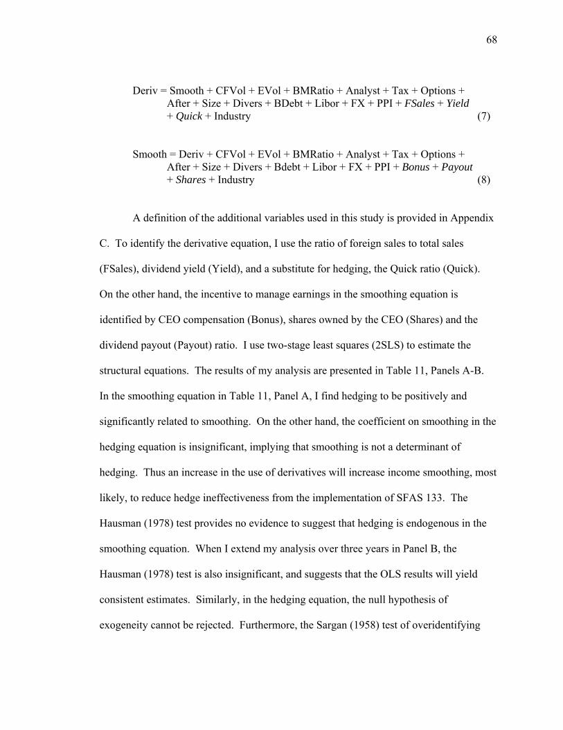
68

Deriv = Smooth + CFVol + EVol + BMRatio + Analyst + Tax + Options + After + Size + Divers + BDebt + Libor + FX + PPI + FSales + Yield + Quick + Industry (7) Smooth = Deriv + CFVol + EVol + BMRatio + Analyst + Tax + Options + After + Size + Divers + Bdebt + Libor + FX + PPI + Bonus + Payout + Shares + Industry (8)

A definition of the additional variables used in this study is provided in Appendix

C. To identify the derivative equation, I use the ratio of foreign sales to total sales

(FSales), dividend yield (Yield), and a substitute for hedging, the Quick ratio (Quick).

On the other hand, the incentive to manage earnings in the smoothing equation is

identified by CEO compensation (Bonus), shares owned by the CEO (Shares) and the

dividend payout (Payout) ratio. I use two-stage least squares (2SLS) to estimate the

structural equations. The results of my analysis are presented in Table 11, Panels A-B.

In the smoothing equation in Table 11, Panel A, I find hedging to be positively and

significantly related to smoothing. On the other hand, the coefficient on smoothing in the

hedging equation is insignificant, implying that smoothing is not a determinant of

hedging. Thus an increase in the use of derivatives will increase income smoothing, most

likely, to reduce hedge ineffectiveness from the implementation of SFAS 133. The

Hausman (1978) test provides no evidence to suggest that hedging is endogenous in the

smoothing equation. When I extend my analysis over three years in Panel B, the

Hausman (1978) test is also insignificant, and suggests that the OLS results will yield

consistent estimates. Similarly, in the hedging equation, the null hypothesis of

exogeneity cannot be rejected. Furthermore, the Sargan (1958) test of overidentifying

69

restrictions provides evidence of the validity of the excluded instruments in the structural

equations.

My results differ from Barton (2001) who finds that hedging and smoothing are

used as substitutes to reduce volatility. On the other hand, my results are similar to the

findings of Pincus and Rajgopal (2002) that hedging is a determinant of smoothing and

not vice versa. However, instead of a negative relation, I find a positive relation between

derivatives and smoothing. If managers use derivatives to hedge or speculate, then they

are likely to engage in a higher level of smoothing to reduce hedge ineffectiveness. In

Panel A, I find the difference in smoothing to be statistically significant and higher in the

period after implementation compared to the period before, consistent with my pooled

OLS results. Turning to the other control variables, dividend payout is significantly

related to smoothing, suggesting that smoothing increases with higher dividend payout

rates. Similarly, the positive foreign sales ratio in the hedging equation is consistent with

previous research. Other coefficients on bank debt, foreign exchange exposure, book-to-

market ratio and firm size are also consistent with the pooled OLS results. Finally, when

I test the sensitivity of my results over the three-year period; my findings in Table 11,

Panel B are qualitatively similar and do not change the tenor of my findings.

As a further test of sensitivity, I break my sample into quintiles by their level of

derivative use to assess whether volatility and smoothing varies with the extent of

hedging. I then rerun the regressions for testing Hypotheses 3-5 to determine whether

Statement 133 has any effect on extreme derivative users (top and bottom 20% of

derivative users). The initial results (means) in Table 12 provide descriptive statistics on

the volatility and smoothing variables relative to derivative non-users. The level of

70

smoothing appears to be inversely related to the level of derivative use; however, large

derivative users (top 20%) appear to engage in the greatest amount of smoothing

compared to other users and non-users. Cash flow volatility shows no systematic pattern

with the level of hedging, but does show that non-users have the highest volatility while

the top 20% has the lowest volatility. If the top 20% of users have the lowest cash flow

volatility and engage in the most smoothing, then one would expect these firms to have

the lowest earnings volatility as well. However, the results show these firms to have high

earnings volatility that is exceeded only by the low derivative users. One possible

explanation is that the standard induces the increase in earnings volatility as the firms

increase the amount of derivatives they use, or these firms may be the ones most affected

by the standard14. To provide further evidence on this issue, I rerun my regressions using

only the top and bottom 20% of derivative users. The results of these regressions are

presented in Table 13, Panels A-C. The results in Panel A show no significant

differences (at 5% level) in hedging relative to volatility and smoothing between firms

that qualify and those that do not qualify for hedge accounting in the bottom and top 20%

of users. In Panel B, among large users, I find the difference in hedging relative to

smoothing to be statistically significant and higher for users that report a transition

adjustment compared to other users in the period after implementation. These results

suggest that large derivative users reported higher transition amounts and were therefore

more likely to have engaged in smoothing to reduce volatility. Finally, in Panel C,

14 I also compute the mean volatility and smoothing before and after by using deciles. I find the top 20% have the highest earnings volatility in the year prior and lowest earnings volatility in the year after. Similarly, mean smoothing is among the lowest in the year before and highest in the year after for this group.

71

although I find no significant differences among low derivative users, my results for large

derivative users suggests otherwise. The difference in hedging relative to cash flow

volatility (smoothing) is significantly lower (higher) for large users that terminated

derivatives compared to other large non-terminating firms. If firms terminate derivatives,

then cash flow volatility and earnings volatility will increase from the unhedged

exposure. Since these firms are more likely to increase their derivative usage, they will

also engage in a greater level of smoothing to reduce earnings volatility. These findings

suggest that firms that are most concerned and affected by SFAS 133 may be the extreme

derivative users that report high transition amounts and are more likely to terminate

derivatives that do not meet the requirements of the standard.

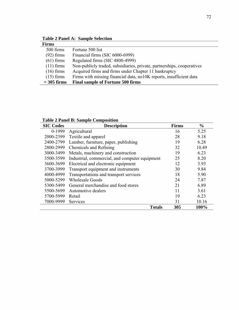
72

Table 2 Panel A: Sample Selection Firms

500 firms Fortune 500 list (92) firms Financial firms (SIC 6000-6999) (61) firms Regulated firms (SIC 4800-4999) (11) firms Non-publicly traded, subsidiaries, private, partnerships, cooperatives (16) firms Acquired firms and firms under Chapter 11 bankruptcy (15) firms Firms with missing financial data, no10K reports, insufficient data

= 305 firms Final sample of Fortune 500 firms Table 2 Panel B: Sample Composition SIC Codes Description Firms %

0-1999 Agricultural 16 5.25 2000-2399 Textile and apparel 28 9.18 2400-2799 Lumber, furniture, paper, publishing 19 6.28 2800-2999 Chemicals and Refining 32 10.49 3000-3499 Metals, machinery and construction 19 6.23 3500-3599 Industrial, commercial, and computer equipment 25 8.20 3600-3699 Electrical and electronic equipment 12 3.93 3700-3999 Transport equipment and instruments 30 9.84 4000-4999 Transportations and transport services 18 5.90 5000-5299 Wholesale Goods 24 7.87 5300-5499 General merchandise and food stores 21 6.89 5500-5699 Automotive dealers 11 3.61 5700-5999 Retail 19 6.23 7000-9999 Services 31 10.16

Totals 305 100%

73

Table 3: Panel A Descriptive Statistics on 261 Derivative Users Derivative Use: Frequency Percent Non-users 44 14.4 Users 261 85.6 Adoption of SFAS 133 for Derivative Users: Early Adoption 8 3.1 Adoption after official date 253 96.9 Type of Risk Hedged: Interest Rate 228 87.7 Foreign Currency 193 73.9 Commodity 99 37.9 Other 37 14.2 Number of Hedged Risks: One risk 67 23.5 Two risks 113 43.4 Three risks 75 28.9 All four risks 11 4.2 Type of Instrument: Forward 201 77.0 Future 46 17.6 Option 136 52.1 Swap 233 89.2 Number of Instruments Used: 1 instrument used 56 21.4 2 instruments 85 32.6 3 instruments 90 34.5 All 4 instruments 30 11.5 Termination of Derivative: Terminated Derivatives 55 21.1 No Termination 206 78.9 Derivative Use After Adoption of SFAS 133: Stopped derivative use 9 3.5 Continued derivative use 251 96.5 Hedge Accounting Treatment: Did not qualify 6 2.3 Qualify for hedge accounting 133 50.9 Partially qualify 122 46.7 Trading Derivatives: Hold Trading Derivatives 14 5.4 No Trading Derivatives 247 94.6 Transition Adjustment: Reported Transition Adjustment 147 56.3 No Transition Adjustment 114 43.7

74

Table 3: Panel B: Descriptive Statistics on 261 Derivative Users (2000-2001) Impact of SFAS 133 Transition Adjustment on Earnings (261 users)

Gain/Loss N Q1 Median Mean Q3 SD Gain 29 1.0 3.0 8.8 8 12.8 Loss 46 -12.0 -3.3 -25.6 -2.0 72.6 Overall 75 -5.0 -1.4 -12.3 2.0 59.6 Impact of SFAS 133 Transition Adjustment on Equity (AOCI) (261 users) Gain 60 3.0 11.0 26.7 44.3 37.7 Loss 72 -16.4 -7.4 -42.3 -3.8 126.9 Overall 132 -9.0 -1 -10.9 7.5 102.7 Notional Values* Year N Q1 Median Mean Q3 SD 2000 189 125 412 1,153 1,147 2,304 2001 188 150.0 575 1,269 1,504 1,921 Overall 377 150 477 1,211 1,353 2,120 * Excludes 30 derivative users without consecutive year observations on FV or NV Table 3 Panel C: Descriptive Statistics of 305 Sample Firms (2000-2001) Variable N Q1 Median Mean Q3 Std. Dev Net Sales 610 4,097 6,893 13,942 14,437 23,941 Income before Ext Items 610 70 226 640 646 1,902 Dependent Variables: User 610 1 1 0.86 1 0.35 Earnings Volatility (2000) 284 .49 0.56 0.97 0.65 3.69 Earnings Volatility (2001) 288 .47 0.56 1.60 0.74 6.70 Cash Flow Volatility (2000) 304 .46 0.80 2.17 1.58 6.79 Cash Flow Volatility (2001) 305 .42 0.79 2.32 1.49 7.92 Smoothing Ratio (2000) 284 .59 1.08 1.64 2.04 1.70 Smoothing Ratio (2001) 288 .64 1.33 2.07 2.66 2.22 Independent Variables: B/M Ratio 610 .85 .362 .469 .612 .546 After 610 0 .5 .5 1 .5 Firm Size ($mil) – Assets 610 3167 6945 14,420 14,298 36,612 Tax 610 0 0 0.27 1 0.44 Bank Debt 610 0 1 0.70 1 0.46 Options (000) 598 613 1,208 2,592 2,463 5,992 Analyst (Number) 610 13 19 20 26 10.4 Diversification 610 0 0.530 0.557 0.959 0.523 Libor 298 -.0049 .0048 .0049 .0209 .0606 FX 298 -.0404 .0001 .0227 .0646 .1825 PPI 297 -.1366 -.0155 .0127 .0726 .4262

75

Table 4: Tests of Differences between Derivative Users and Non-Users (2000-2001) Mean Medians test of differences Wilcoxon rank-sum test

Variable User Non-User User Non-User Predict t stat p-value z-stat p-value Evol 0.96 0.97 0.56 0.59 U>NU 0.01 0.497 2.44 0.007 CFVol 1.96 2.30 0.78 0.91 NU>U 0.46 0.322 0.86 0.194 Smooth 1.90 1.64 1.17 1.09 U>NU -1.09 0.138 0.30 0.381 Bdebt 0.72 0.52 1 1 U>NU -3.46 0.000 -3.71 0.000 BMRatio 0.46 0.57 0.37 0.35 NU>U 1.72 0.044 0.79 0.215 Analyst 2.88 2.72 2.94 2.94 U>NU -2.11 0.019 -1.61 0.054 Tax 0.29 0.11 0 0 U>NU -4.50 0.000 -3.49 0.000 Options 7.18 6.86 7.11 7.10 U-N=0 -2.43 0.015 -1.40 0.162 Size 8.94 8.24 8.90 8.45 U>NU -5.75 0.000 -5.06 0.000 Divers .585 .388 .572 .162 U>NU -3.294 0.000 -3.356 0.000 Notes: All variables except indicator variables, options, analyst and firm size have been winsorized at the 1% and 99% levels. P-values in bold reflect significance at the .01 and .05 levels respectively depending on two-tailed or one-tailed prediction. Definition of variables is provided in Appendix C. Test of differences not computed on exposure coefficients

76

Table 5: Correlations between Dependent Variables and Independent Variables (2000-2001) After BMRatio User NV Evol Cfvol Smooth BDebt Size Tax Options Divers AnalystAfter 1 .000 .000 .087 .045 -.004 .082* .000 .031 -.015 .067 .010 -.045BMRatio -.047 1 -.032 -.187** .130** .214** .379** .048 -.111** -.019 -.289** .020 -.409**User .000 -.090* 1 . -.102* -.035 .013 .150** .205** .141** .058 .136** .066NV .028 -.106* . 1 -.062 -.010 -.009 .188** -.026 -.030 .042 .032 -.072Evol .082 .101* -.000 .026 1 .213** .115** -.005 -.031 -.088* -.028 -.077 -.106*Cfvol -.001 .144** -.023 -.009 .019 1 .693** -.016 -.226** -.024 -.118** -.064 -.262**Smooth .107* .311** .046 .056 .089* .289** 1 -.002 -.207** .037 -.186** -.055 -.294**BDebt .000 .028 .150** .129** -.079 -.001 .015 1 .056 .056 .017 -.021 .005Size .037 -.097* .227** -.073 .008 -.064 -.133** .073 1 -.042 .402** .245** .533**Tax -.015 -.057 .141** -.096 -.092* .008 .036 .056 -.045 1 -.108** -.024 -.012Options .056 -.217** .099* .109* .022 .044 -.098* .027 .409** -.089* 1 .009 .404**Divers .011 -.065 .132** -.014 -.039 -.057 -.047 -.019 .277** -.025 .029 1Analyst -.036 -.374** .094* -.023 -.036 -.081* -.241** -.028 .520** -.004 .420** -.003 1Notes: All variables except indicator variables, options, analyst and firm size have been winsorized at the 1% and 99% levels. Values below the diagonal reflect Pearson's correlation and values above the diagonal reflect Spearman rank correlation. **, * denote 1% and 5% significant levels respectively based on two-tailed tests. Correlations of exposure coefficients omitted

77

Table 6 Determinants of Incentives for Derivatives between Users and Non-Users, 1999-2001

Independent Variables Sign Model 1 (00-01): Coeff. (z-stat)

Model 2 (99-01): Coeff. (z-stat)

Intercept +/- -4.709 (-5.17)***

-4.579 (-6.19)***

Evol + 0.014 (0.32)

0.021 (0.56)

CFVol + 0.007 (0.54)

0.008 (0.71)

Smooth - 0.194 (2.64)***

0.202 (3.46)***

After + -0.179 (-1.01)

-0.213 (-1.41)*

BDebt + 0.665 (3.52)***

0.660 (4.36)***

B/M Ratio - -0.658 (-3.38)***

-0.557 (-3.20)***

Analyst +/- -0.339 (-2.05)**

-0.246 (-1.72)*

Tax +/- 0.678 (2.81)***

0.707 (3.59)***

Options +/- 0.227 (3.06)***

0.204 (3.27)***

Size +/- 0.486 (4.17)***

0.451 (4.67)***

Divers +/- -0.072 (-0.34)

-0.027 (-0.16)

Libor +/- 3.730 (1.75)*

3.697 (2.13)**

FX +/- 0.699 (1.28)

0.729 (1.62)

PPI +/- 1.096 (3.34)***

1.017 (3.72)***

Observations 409 610 LR Chi-sq 125 175

P-value 0.0000 0.0000 Pseudo R-Square 0.336 0.329

% Correctly Predicted 83.6% 84.6% Notes: All variables except dummy variables and firm size are winsorized at the 1% 99% levels. ***, **, * denote the 1%, 5% and 10% significance levels respectively based on one-tailed tests, two-tailed otherwise. Coefficients on industry dummies are not reported. T-statistics are based on White heteroskedasticity robust standard-errors

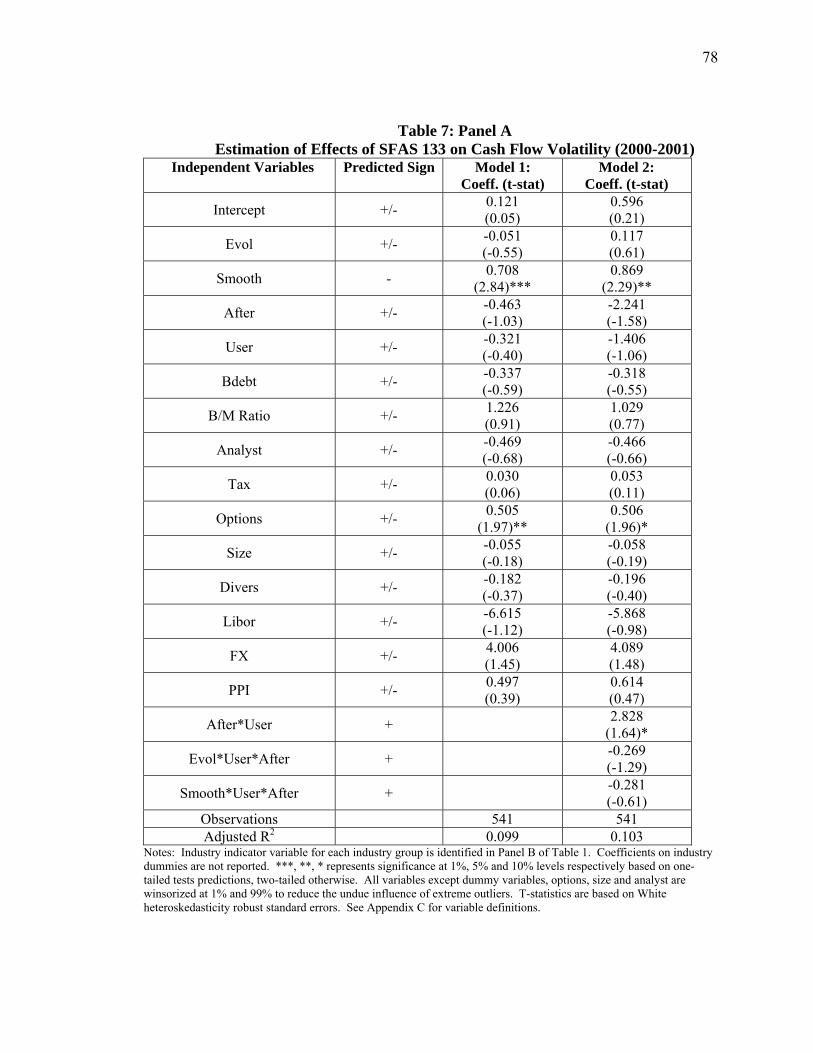
78

Table 7: Panel A Estimation of Effects of SFAS 133 on Cash Flow Volatility (2000-2001)

Independent Variables Predicted Sign Model 1: Coeff. (t-stat)

Model 2: Coeff. (t-stat)

Intercept +/- 0.121 (0.05)

0.596 (0.21)

Evol +/- -0.051 (-0.55)

0.117 (0.61)

Smooth - 0.708 (2.84)***

0.869 (2.29)**

After +/- -0.463 (-1.03)

-2.241 (-1.58)

User +/- -0.321 (-0.40)

-1.406 (-1.06)

Bdebt +/- -0.337 (-0.59)

-0.318 (-0.55)

B/M Ratio +/- 1.226 (0.91)

1.029 (0.77)

Analyst +/- -0.469 (-0.68)

-0.466 (-0.66)

Tax +/- 0.030 (0.06)

0.053 (0.11)

Options +/- 0.505 (1.97)**

0.506 (1.96)*

Size +/- -0.055 (-0.18)

-0.058 (-0.19)

Divers +/- -0.182 (-0.37)

-0.196 (-0.40)

Libor +/- -6.615 (-1.12)

-5.868 (-0.98)

FX +/- 4.006 (1.45)

4.089 (1.48)

PPI +/- 0.497 (0.39)

0.614 (0.47)

After*User + 2.828 (1.64)*

Evol*User*After + -0.269 (-1.29)

Smooth*User*After + -0.281 (-0.61)

Observations 541 541 Adjusted R2 0.099 0.103

Notes: Industry indicator variable for each industry group is identified in Panel B of Table 1. Coefficients on industry dummies are not reported. ***, **, * represents significance at 1%, 5% and 10% levels respectively based on one-tailed tests predictions, two-tailed otherwise. All variables except dummy variables, options, size and analyst are winsorized at 1% and 99% to reduce the undue influence of extreme outliers. T-statistics are based on White heteroskedasticity robust standard errors. See Appendix C for variable definitions.

79

Table 7: Panel B Estimation of Effects of SFAS 133 on Earnings Volatility (2000-2001)

Independent Variables Predicted Sign Model 1: Coeff. (t-stat)

Model 2: Coeff. (t-stat)

Intercept +/- 0.345 (0.31)

0.308 (0.32)

CFVol +/- -0.008 (-0.56)

0.005 (0.28)

Smooth - 0.050 (0.99)

0.077 (1.17)

After + 0.321 (1.93)**

0.557 (1.37)*

User + 0.172 (0.53)

0.325 (1.16)

Bdebt +/- -0.562 (-1.95)*

-0.564 (-1.96)**

B/M Ratio +/- 0.549 (1.26)

0.514 (1.16)

Analyst +/- -0.073 (-0.38)

-0.093 (-0.47)

Tax +/- -0.426 (-2.76)***

-0.435 (-2.74)***

Options +/- 0.033 (0.43)

0.029 (0.38)

Size +/- 0.120 (1.20)

0.119 (1.18)

Divers +/- -0.352 (-1.48)

-0.370 (-1.52)

Libor +/- 1.472 (0.63)

1.454 (0.62)

FX +/- -0.227 (-0.30)

-0.217 (-0.29)

PPI +/- 0.027 (0.06)

0.005 (0.01)

After*User + -0.095 (-0.22)

CFVol*User*After + -0.070 (-1.43)*

Smooth*User*After + -0.037 (-0.40)

Observations 541 541 Adjusted R2 0.013 0.011

Notes: Industry indicator variable for each industry group is identified in Panel B of Table 1. Coefficients on industry dummies are not reported. ***, **, * represents significance at 1%, 5% and 10% levels respectively based on one-tailed tests predictions, two-tailed otherwise. All variables except dummy variables, options, size and analyst are winsorized at 1% and 99% to reduce the undue influence of extreme outliers. T-statistics are based on White heteroskedasticity robust standard errors. See Appendix C for variable definitions.

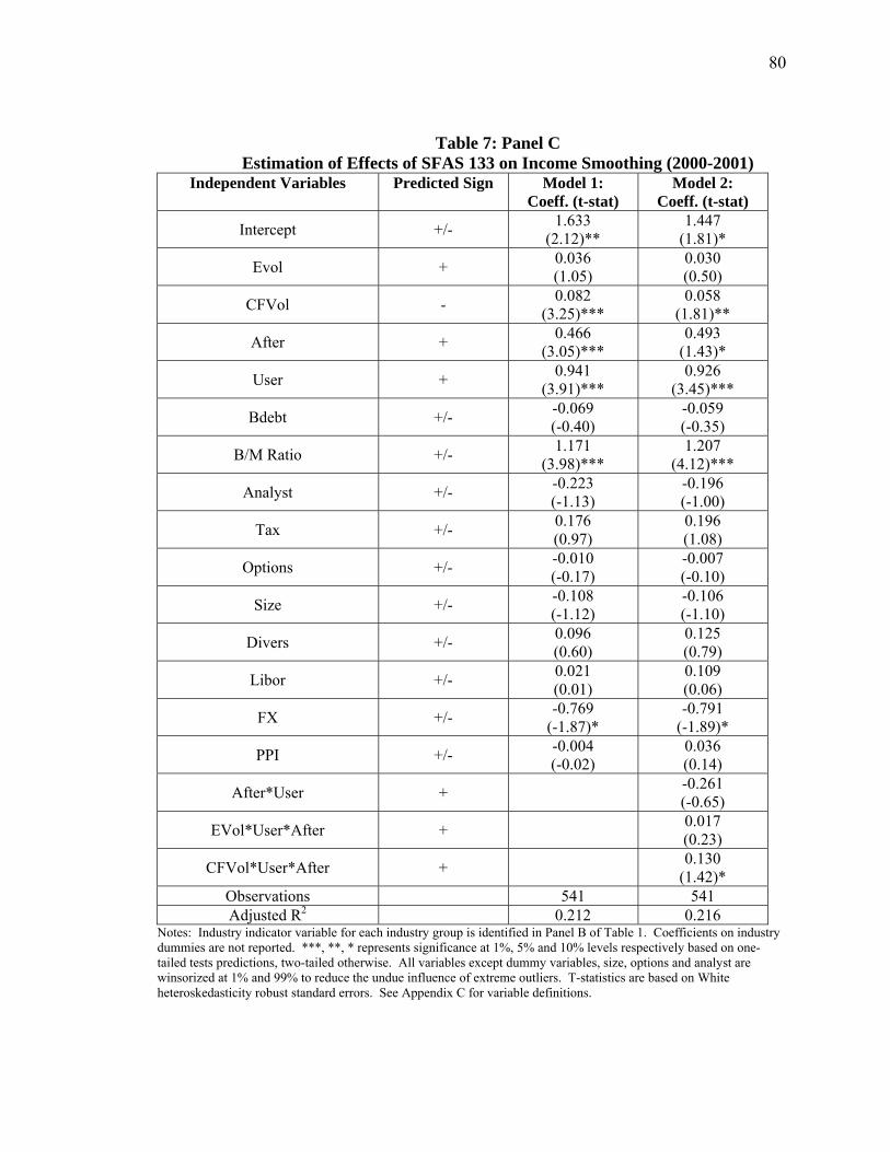
80

Table 7: Panel C Estimation of Effects of SFAS 133 on Income Smoothing (2000-2001)

Independent Variables Predicted Sign Model 1: Coeff. (t-stat)

Model 2: Coeff. (t-stat)

Intercept +/- 1.633 (2.12)**

1.447 (1.81)*

Evol + 0.036 (1.05)

0.030 (0.50)

CFVol - 0.082 (3.25)***

0.058 (1.81)**

After + 0.466 (3.05)***

0.493 (1.43)*

User + 0.941 (3.91)***

0.926 (3.45)***

Bdebt +/- -0.069 (-0.40)

-0.059 (-0.35)

B/M Ratio +/- 1.171 (3.98)***

1.207 (4.12)***

Analyst +/- -0.223 (-1.13)

-0.196 (-1.00)

Tax +/- 0.176 (0.97)

0.196 (1.08)

Options +/- -0.010 (-0.17)

-0.007 (-0.10)

Size +/- -0.108 (-1.12)

-0.106 (-1.10)

Divers +/- 0.096 (0.60)

0.125 (0.79)

Libor +/- 0.021 (0.01)

0.109 (0.06)

FX +/- -0.769 (-1.87)*

-0.791 (-1.89)*

PPI +/- -0.004 (-0.02)

0.036 (0.14)

After*User + -0.261 (-0.65)

EVol*User*After + 0.017 (0.23)

CFVol*User*After + 0.130 (1.42)*

Observations 541 541 Adjusted R2 0.212 0.216

Notes: Industry indicator variable for each industry group is identified in Panel B of Table 1. Coefficients on industry dummies are not reported. ***, **, * represents significance at 1%, 5% and 10% levels respectively based on one-tailed tests predictions, two-tailed otherwise. All variables except dummy variables, size, options and analyst are winsorized at 1% and 99% to reduce the undue influence of extreme outliers. T-statistics are based on White heteroskedasticity robust standard errors. See Appendix C for variable definitions.

81

Table 7 Panel D Estimation of Effects of SFAS 133 on Cash Flow Volatility (1999-2001)

Independent Variables Predicted Sign Model 1: Coeff. (t-stat)

Model 2: Coeff. (t-stat)

Intercept +/- 1.117 (0.53)

1.249 (0.58)

Evol +/- -0.041 (-0.66)

0.025 (0.28)

Smooth - 0.671 (3.66)***

0.741 (3.29)***

After +/- -0.398 (-1.03)

-1.306 (-1.50)

User +/- -0.066 (-0.11)

-0.463 (-0.59)

Bdebt +/- 0.047 (0.12)

0.051 (0.13)

B/M Ratio +/- 0.562 (0.53)

0.483 (0.46)

Analyst +/- -0.376 (-0.70)

-0.369 (-0.68)

Tax +/- 0.422 (0.95)

0.424 (0.96)

Options +/- 0.406 (1.82)*

0.403 (1.82)*

Size +/- -0.090 (-0.43)

-0.094 (-0.45)

Divers +/- -0.409 (-0.97)

-0.402 (-0.95)

Libor +/- -6.238 (-1.45)

-5.986 (-1.37)

FX +/- 2.473 (1.27)

2.504 (1.27)

PPI +/- 0.391 (0.43)

0.434 (0.47)

After*User + 1.549 (1.39)*

Evol*User*After + -0.151 (-1.28)

Smooth*User*After + -0.172 (-0.48)

Observations 806 806 Adjusted R2 0.087 0.086

Notes: Industry indicator variable for each industry group is identified in Panel B of Table 1. Coefficients on industry dummies are not reported. ***, **, * represents significance at 1%, 5% and 10% levels respectively based on one-tailed tests predictions, two-tailed otherwise. All variables except dummy variables, size, options and analyst are winsorized at 1% and 99% to reduce the undue influence of extreme outliers. T-statistics are based on White heteroskedasticity robust standard errors. See Appendix C for variable definitions.

82

Table 7 Panel E Estimation of Effects of SFAS 133 on Earnings Volatility (1999-2001)

Independent Variables Predicted Sign Model 1: Coeff. (t-stat)

Model 2: Coeff. (t-stat)

Intercept +/- 0.991 (1.11)

0.945 (1.19)

CFVol +/- -0.006 (-0.68)

0.002 (0.19)

Smooth - 0.044 (1.03)

0.049 (0.96)

After + 0.233 (1.44)*

0.510 (1.24)

User + 0.226 (0.97)

0.344 (1.72)**

Bdebt +/- -0.423 (-1.98)**

-0.428 (-1.98)**

B/M Ratio +/- 0.395 (1.18)

0.381 (1.13)

Analyst +/- -0.118 (-0.55)

-0.131 (-0.61)

Tax +/- -0.268 (-1.88)*

-0.277 (-1.91)*

Options +/- -0.019 (-0.24)

-0.020 (-0.26)

Size +/- 0.140 (1.79)*

0.141 (1.78)*

Divers +/- -0.437 (-2.17)**

-0.444 (-2.18)**

Libor +/- 2.520 (1.33)

2.479 (1.30)

FX +/- -0.350 (-0.58)

-0.332 (-0.55)

PPI +/- 0.013 (0.04)

-0.003 (-0.01)

After*User + -0.210 (-0.45)

CFVol*User*After + -0.064 (-1.60)*

Smooth*User*After + -0.004 (-0.05)

Observations 806 806 Adjusted R2 0.017 0.016

Notes: Industry indicator variable for each industry group is identified in Panel B of Table 1. Coefficients on industry dummies are not reported. ***, **, * represents significance at 1%, 5% and 10% levels respectively based on one-tailed tests predictions, two-tailed otherwise. All variables except dummy variables, size, options and analyst are winsorized at 1% and 99% to reduce the undue influence of extreme outliers. T-statistics are based on White heteroskedasticity robust standard errors. See Appendix C for variable definitions.

83

Table 7 Panel F Estimation of Effects of SFAS 133 on Income Smoothing (1999-2001)

Independent Variables Predicted Sign Model 1: Coeff. (t-stat)

Model 2: Coeff. (t-stat)

Intercept +/- 1.332 (2.17)**

1.225 (1.95)*

Evol + 0.032 (1.05)

0.030 (0.68)

CFVol - 0.076 (3.85)***

0.060 (2.79)***

After + 0.362 (2.63)***

0.383 (1.23)

User + 0.864 (4.66)***

0.857 (4.42)***

Bdebt +/- -0.121 (-0.90)

-0.109 (-0.82)

B/M Ratio +/- 1.327 (5.21)***

1.342 (5.28)***

Analyst +/- -0.220 (-1.30)

-0.199 (-1.19)

Tax +/- 0.050 (0.36)

0.069 (0.49)

Options +/- 0.042 (0.72)

0.044 (0.76)

Size +/- -0.073 (-0.94)

-0.072 (-0.93)

Divers +/- 0.009 (0.07)

0.023 (0.17)

Libor +/- -0.014 (-0.01)

0.051 (0.04)

FX +/- -0.500 (-1.54)

-0.535 (-1.62)

PPI +/- 0.085 (0.41)

0.112 (0.53)

After*User + -0.238 (-0.65)

EVol*User*After + 0.010 (0.18)

CFVol*User*After + 0.123 (1.48)*

Observations 806 806 Adjusted R2 0.212 0.216

Notes: Industry indicator variable for each industry group is identified in Panel B of Table 1. Coefficients on industry dummies are not reported. ***, **, * represents significance at 1%, 5% and 10% levels respectively based on one-tailed tests predictions, two-tailed otherwise. All variables except dummy variables, size, options and analyst are winsorized at 1% and 99% to reduce the undue influence of extreme outliers. T-statistics are based on White heteroskedasticity robust standard errors. See Appendix C for variable definitions.

84

Table 8 Estimation of Effects of SFAS 133 on Derivatives (2000-2001)

Independent Variables Predicted Sign User (Probit) Coeff. (z-stat)

NV (Heckman) Coeff. (z-stat)

Intercept +/- -0.561 (-0.88)

0.033 (0.26)

EVol + 0.023 (0.85)

0.002 (0.40)

CFVol +/- -0.001 (-0.12)

0.001 (0.54)

Smooth + 0.117 (3.28)***

0.012 (1.82)**

After +/- -0.165 (-1.21)

-0.039 (-1.64)*

DNQ +/- 0.465 (2.58)***

0.077 (2.39)**

BDebt +/- 0.534 (3.94)***

0.079 (2.50)**

B/M Ratio +/- -0.203 (-1.19)

-0.022 (-0.73)

Analyst +/- -0.094 (-0.73)

-0.031 (-1.49)

Tax +/- 0.454 (3.29)***

Options +/- 0.163 (2.66)***

0.039 (3.52)***

Size +/- -0.069 (-0.89)

-0.030 (-2.27)**

Divers +/- 0.004 (0.03)

-0.013 (-0.67)

Libor +/- -8.708 (-3.61)***

-0.189 (-0.48)

FX +/- -0.099 (-0.27)

-0.110 (-2.08)**

PPI +/- -1.010 (-3.48)***

-0.073 (-1.50)

Mills +/- 0.101 (1.34)

Observations 541 541 Pseudo R2 0.134

Notes: Industry indicator variable for each industry group is identified in Panel B of Table 1. Coefficients on industry dummies are not reported. ***, **, * represents significance at 1%, 5% and 10% levels respectively based on one-tailed tests predictions, two-tailed otherwise. All variables except dummy variables, size, options and analyst are winsorized at 1% and 99% to reduce the undue influence of extreme outliers. Dependent variable for probit model equals 1 for derivative user; 0 otherwise. See Appendix A for variable definitions.

85

Table 9 Panel A Effects of Hedge Accounting Treatment on Derivatives (2000-2001)

Independent Variables Predicted Sign Model 1: Coeff. (t-stat)

Model 2: Coeff. (t-stat)

Intercept +/- 0.104 (1.09)

0.084 (0.86)

EVol + 0.002 (0.37)

0.011 (3.32)***

CFVol + 0.000 (0.07)

-0.000 (-0.10)

Smooth - 0.009 (1.90)*

0.008 (0.82)

After +/- -0.025 (-1.27)

-0.010 (-0.39)

DNQ +/- 0.057 (2.31)**

0.044 (1.54)

BDebt + 0.053 (2.55)**

0.053 (2.50)**

B/M Ratio +/- -0.021 (-0.83)

-0.029 (-1.22)

Analyst +/- -0.016 (-1.03)

-0.015 (-0.96)

Tax +/- -0.015 (-0.96)

-0.014 (-0.92)

Options +/- 0.029 (2.79)***

0.030 (2.79)***

Size +/- -0.026 (-1.79)*

-0.025 (-1.68)*

Divers +/- -0.010 (-0.57)

-0.009 (-0.48)

Libor +/- 0.106 (0.36)

0.130 (0.45)

FX +/- -0.106 (-1.85)*

-0.100 (-1.68)*

PPI +/- -0.028 (-1.02)

-0.024 (-0.90)

CFVol*After +/- -0.003 (-0.53)

CFVol*DNQ*After + 0.007 (0.82)

EVol*After +/- -0.018 (-3.65)***

EVol*DNQ*After + 0.004 (0.70)

Smooth*After +/- 0.004 (0.34)

Smooth*DNQ*After + -0.001 (-0.07)

Observations 339 339 Adjusted R2 0.124 0.119

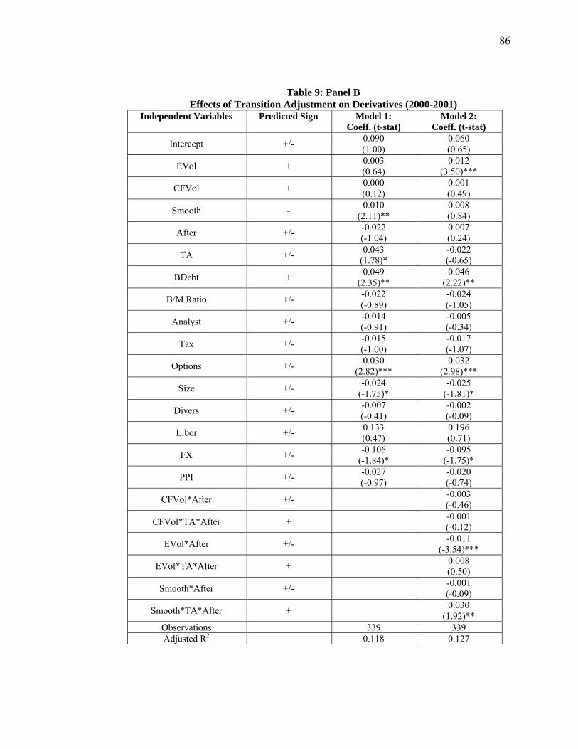
86

Table 9: Panel B Effects of Transition Adjustment on Derivatives (2000-2001)

Independent Variables Predicted Sign Model 1: Coeff. (t-stat)

Model 2: Coeff. (t-stat)

Intercept +/- 0.090 (1.00)

0.060 (0.65)

EVol + 0.003 (0.64)

0.012 (3.50)***

CFVol + 0.000 (0.12)

0.001 (0.49)

Smooth - 0.010 (2.11)**

0.008 (0.84)

After +/- -0.022 (-1.04)

0.007 (0.24)

TA +/- 0.043 (1.78)*

-0.022 (-0.65)

BDebt + 0.049 (2.35)**

0.046 (2.22)**

B/M Ratio +/- -0.022 (-0.89)

-0.024 (-1.05)

Analyst +/- -0.014 (-0.91)

-0.005 (-0.34)

Tax +/- -0.015 (-1.00)

-0.017 (-1.07)

Options +/- 0.030 (2.82)***

0.032 (2.98)***

Size +/- -0.024 (-1.75)*

-0.025 (-1.81)*

Divers +/- -0.007 (-0.41)

-0.002 (-0.09)

Libor +/- 0.133 (0.47)

0.196 (0.71)

FX +/- -0.106 (-1.84)*

-0.095 (-1.75)*

PPI +/- -0.027 (-0.97)

-0.020 (-0.74)

CFVol*After +/- -0.003 (-0.46)

CFVol*TA*After + -0.001 (-0.12)

EVol*After +/- -0.011 (-3.54)***

EVol*TA*After + 0.008 (0.50)

Smooth*After +/- -0.001 (-0.09)

Smooth*TA*After + 0.030 (1.92)**

Observations 339 339 Adjusted R2 0.118 0.127

87

Table 9: Panel C Effects of Hedge Termination on Derivatives (2000-2001)

Independent Variables Predicted Sign Model 1: Coeff. (t-stat)

Model 2: Coeff. (t-stat)

Intercept +/- 0.071 (0.79)

0.042 (0.44)

EVol + 0.002 (0.50)

0.011 (3.43)***

CFVol + 0.000 (0.13)

0.000 (0.20)

Smooth - 0.010 (1.93)*

0.008 (0.90)

After +/- 0.001 (0.07)

0.007 (0.27)

Term +/- -0.000 (-0.00)

0.029 (0.61)

Bdebt + 0.052 (2.50)**

0.051 (2.43)***

B/M Ratio +/- -0.022 (-0.88)

-0.031 (-1.31)

Analyst +/- -0.018 (-1.14)

-0.018 (-1.12)

Tax +/- -0.014 (-0.88)

-0.011 (-0.74)

Options +/- 0.031 (2.83)***

0.032 (2.89)***

Size +/- -0.021 (-1.52)

-0.021 (-1.44)

Divers +/- -0.008 (-0.44)

-0.006 (-0.29)

Libor +/- 0.153 (0.54)

0.172 (0.62)

FX +/- -0.110 (-1.90)*

-0.111 (-1.88)*

PPI +/- -0.023 (-0.85)

-0.026 (-0.99)

CFVol*After +/- 0.003 (0.54)

CFVol*Term*After + -0.011 (-1.13)

EVol*After +/- -0.016 (-3.09)***

EVol*Term*After + -0.007 (-0.10)

Smooth*After +/- 0.003 (0.28)

Smooth*Term*After + -0.004 (-0.23)

Observations 339 339 Adjusted R2 0.109 0.107

88

Table 9 Panel D Effects of Hedge Accounting Treatment on Derivatives (1999-2001)

Independent Variables Predicted Sign Model 1: Coeff. (t-stat)

Model 2: Coeff. (t-stat)

Intercept +/- 0.056 (0.72)

0.040 (0.51)

EVol + 0.002 (0.79)

0.006 (2.06)**

CFVol + -0.000 (-0.38)

-0.000 (-0.59)

Smooth - 0.009 (2.59)***

0.008 (1.54)*

After +/- -0.015 (-0.89)

-0.008 (-0.34)

DNQ +/- 0.053 (2.25)**

0.042 (1.48)

BDebt + 0.049 (2.84)***

0.048 (2.79)***

B/M Ratio +/- -0.020 (-1.07)

-0.022 (-1.20)

Analyst +/- -0.010 (-0.79)

-0.010 (-0.75)

Tax +/- -0.008 (-0.67)

-0.008 (-0.68)

Options +/- 0.019 (1.79)*

0.019 (1.84)*

Size +/- -0.015 (-1.25)

-0.014 (-1.18)

Divers +/- -0.005 (-0.29)

-0.004 (-0.26)

Libor +/- 0.045 (0.21)

0.052 (0.24)

FX +/- -0.087 (-2.08)**

-0.085 (-1.97)**

PPI +/- -0.027 (-1.33)

-0.026 (-1.26)

CFVol*After +/- -0.002 (-0.40)

CFVol*DNQ*After + 0.005 (0.74)

EVol*After +/- -0.012 (-2.75)***

EVol*DNQ*After + 0.003 (0.56)

Smooth*After +/- 0.003 (0.47)

Smooth*DNQ*After + 0.000 (0.04)

Observations 503 503 Adjusted R2 0.113 0.108

89

Table 9: Panel E Effects of Transition Adjustment on Derivatives (1999-2001)

Independent Variables Predicted Sign Model 1: Coeff. (t-stat)

Model 2: Coeff. (t-stat)

Intercept +/- 0.047 (0.63)

0.023 (0.30)

EVol + 0.003 (1.03)

0.006 (2.08)**

CFVol + -0.000 (-0.29)

-0.000 (-0.11)

Smooth - 0.010 (2.76)***

0.008 (1.60)*

After +/- -0.011 (-0.62)

0.009 (0.37)

TA +/- 0.039 (1.70)*

-0.024 (-0.71)

BDebt + 0.046 (2.68)***

0.043 (2.52)**

B/M Ratio +/- -0.021 (-1.12)

-0.018 (-1.05)

Analyst +/- -0.009 (-0.69)

-0.004 (-0.27)

Tax +/- -0.009 (-0.72)

-0.010 (-0.83)

Options +/- 0.019 (1.80)*

0.020 (1.93)*

Size +/- -0.014 (-1.20)

-0.014 (-1.22)

Divers +/- -0.003 (-0.16)

0.000 (0.02)

Libor +/- 0.062 (0.29)

0.096 (0.45)

FX +/- -0.087 (-2.07)**

-0.082 (-2.02)**

PPI +/- -0.027 (-1.30)

-0.022 (-1.09)

CFVol*After +/- -0.001 (-0.12)

CFVol*TA*After + -0.001 (-0.11)

EVol*After +/- -0.011 (-2.64)***

EVol*TA*After + 0.007 (0.50)

Smooth*After +/- -0.001 (-0.18)

Smooth*TA*After + 0.029 (1.87)**

Observations 503 503 Adjusted R2 0.109 0.113

90

Table 9: Panel F Effects of Hedge Termination on Derivatives (1999-2001)

Independent Variables Predicted Sign Model 1: Coeff. (t-stat)

Model 2: Coeff. (t-stat)

Intercept +/- 0.035 (0.47)

0.014 (0.18)

EVol + 0.002 (0.84)

0.006 (2.06)**

CFVol + -0.000 (-0.30)

-0.000 (-0.39)

Smooth - 0.009 (2.60)***

0.008 (1.61)*

After +/- 0.011 (0.79)

0.010 (0.49)

Term +/- -0.008 (-0.30)

0.012 (0.30)

Bdebt + 0.048 (2.80)***

0.047 (2.73)***

B/M Ratio +/- -0.020 (-1.07)

-0.022 (-1.22)

Analyst +/- -0.011 (-0.85)

-0.010 (-0.80)

Tax +/- -0.008 (-0.64)

-0.007 (-0.61)

Options +/- 0.019 (1.80)*

0.020 (1.89)*

Size +/- -0.012 (-1.02)

-0.011 (-0.97)

Divers +/- -0.003 (-0.21)

-0.002 (-0.15)

Libor +/- 0.074 (0.34)

0.077 (0.36)

FX +/- -0.089 (-2.09)**

-0.090 (-2.09)**

PPI +/- -0.024 (-0.21)

-0.026 (-1.27)

CFVol*After +/- 0.004 (0.80)

CFVol*Term*After + -0.008 (-0.92)

EVol*After +/- -0.010 (-2.32)**

EVol*Term*After + -0.007 (-0.12)

Smooth*After +/- 0.003 (0.49)

Smooth*Term*After + -0.004 (-0.23)

Observations 503 503 Adjusted R2 0.104 0.099

91

Table 10 Panel A: Fixed Effects Model of SFAS 133 on Cash Flow Volatility (1999-2001)

Independent Variables

Predicted Sign Model 1 (2000-2001): Coeff. (t-stat)

Model 2 (2000-2001): Coeff. (t-stat)

Model 3 (1999-2001): Coeff. (t-stat)

Intercept +/- 0.587 (1.04)

-24.926 (-1.22)

0.819 (0.07)

EVol + -0.006 (-0.02)

-0.045 (-0.18)

-0.044 (-0.27)

Smooth - 0.941 (3.43)***

0.951 (3.19)***

0.533 (2.86)***

After +/- -2.326 (-2.01)**

-2.485 (-1.97)**

-1.405 (-1.38)

User +/- Dropped Dropped -0.637 (-0.10)

BDebt Dropped Dropped

BMRatio +/- 2.256 (1.19)

1.627 (1.37)

Analyst +/- 2.519 (1.53)

0.111 (0.11)

Tax +/- 1.620 (1.10)

0.556 (0.58)

Options +/- 0.325 (0.46)

0.556 (1.30)

Size +/- 2.212 (0.96)

0.037 (0.03)

Fsales +/- -22.119 (-1.93)*

-19.149 (-4.06)***

Divers +/- 0.381 (0.09)

-0.271 (-0.13)

After*User + 2.796 (2.00)**

2.814 (1.89)**

1.410 (1.17)

EVol*After*User + -0.076 (-0.24)

0.035 (0.11)

-0.047 (-0.20)

Smooth*After*User + -0.273 (-0.98)

-0.265 (-0.89)

0.013 (0.06)

Observations 572 546 812 Overall R2 0.083 0.031 0.022

***,**,* represents significance at 1%, 5%, and 10% based on one-tailed predictions, two-tailed otherwise.

92

Table 10 Panel B: Fixed Effects Model of SFAS 133 on Earnings Volatility (1999-2001) Independent Variables Predicted

Sign Model 1 (2000-2001): Coeff. (t-stat)

Model 2 (2000-2001): Coeff. (t-stat)

Model 3 (1999-2001): Coeff. (t-stat)

Intercept +/- 0.770 (3.87)***

11.691 (1.61)

7.206 (1.79)*

CFVol + 0.009 (0.33)

0.018 (0.66)

-0.005 (-0.28)

Smooth - 0.021 (0.20)

-0.031 (-0.28)

0.029 (0.45)

After + 0.533 (1.25)

0.860 (1.91)**

0.682 (1.91)**

User + Dropped Dropped 0.218 (0.10)

Bdebt Dropped Dropped

BMRatio +/- 1.597 (2.39)**

0.749 (1.80)*

Analyst +/- 0.943 (1.57)

0.050 (0.13)

Tax +/- -1.462 (-2.84)***

-0.640 (-1.93)*

Options +/- -0.326 (-1.28)

-0.245 (-1.64)

Size +/- -1.486 (-1.82)*

-0.662 (-1.57)

Fsales +/- 2.049 (0.50)

1.651 (0.98)

Divers +/- 1.701 (1.11)

0.526 (0.74)

After*User + -0.207 (-0.41)

-0.415 (-0.80)

-0.445 (-1.08)

CFVol*After*User + -0.081 (-1.01)

-0.116 (-1.34)*

-0.021 (-0.34)

Smooth*After*User + 0.018 (0.16)

0.085 (0.74)

0.018 (0.22)

Observations 572 546 812 Overall R2 0.010 0.003 0.003

***,**,* represents significance at 1%, 5%, and 10% based on one-tailed predictions, two-tailed otherwise.

93

Table 10 Panel C: Fixed Effects Model of SFAS 133 on Income Smoothing (1999-2001) Independent Variables Predicted

Sign Model 1 (2000-2001): Coeff. (t-stat)

Model 2 (2000-2001): Coeff. (t-stat)

Model 3 (1999-2001): Coeff. (t-stat)

Intercept +/- 1.491 (13.45)***

9.355 (1.68)*

5.274 (1.65)*

EVol + 0.049 (0.70)

0.035 (0.50)

0.034 (0.76)

CFVol + 0.050 (2.54)***

0.047 (2.35)***

0.034 (2.46)***

After + 0.292 (0.88)

0.494 (1.43)*

0.411 (1.45)*

User + Dropped Dropped 0.131 (0.08)

Bdebt Dropped Dropped

BMRatio +/- 1.024 (1.99)**

1.169 (3.59)***

Analyst +/- -0.219 (-0.48)

-0.355 (-1.19)

Tax +/- 0.245 (0.61)

0.169 (0.63)

Options +/- 0.153 (0.79)

0.129 (1.08)

Size +/- -1.041 (-1.66)*

-0.539 (-1.61)

FSales +/- 0.131 (0.04)

1.988 (1.49)

Divers +/- 0.463 (0.39)

0.068 (0.12)

After*User + 0.112 (0.30)

-0.039 (-0.10)

-0.085 (-0.27)

EVol*After*User + -0.050 (-0.56)

-0.037 (-0.41)

-0.023 (-0.35)

CFVol*After*User + 0.059 (1.03)

0.059 (0.99)

0.058 (1.25)

Observations 572 546 812 Overall R2 0.104 0.114 0.111

***,**,* represents significance at 1%, 5%, and 10% based on one-tailed predictions, two-tailed otherwise.

94

Table 10 Panel D : Fixed Effects Model of SFAS 133 on Hedge Acct. Treatment (1999-2001) Independent Variables Predicted

Sign Model 1 (2000-2001): Coeff. (t-stat)

Model 2 (2000-2001): Coeff. (t-stat)

Model 3 (1999-2001): Coeff. (t-stat)

Intercept +/- 0.132 (13.69)***

0.753 (2.47)**

0.301 (1.60)

EVol + -0.009 (-2.47)***

-0.008 (-1.99)**

-0.006 (-2.23)**

CFVol + -0.000 (-0.22)

0.000 (0.02)

0.000 (0.23)

Smooth - 0.000 (0.08)

0.001 (0.23)

-0.006 (-1.67)**

After +/- -0.010 (-0.68)

-0.007 (-0.40)

0.001 (0.05)

Qualify +/- 0.015 (0.69)

0.028 (1.22)

0.001 (0.04)

BDebt +/- Dropped Dropped

BMRatio +/- -0.021 (-0.72)

-0.021 (-1.02)

Analyst +/- 0.022 (0.83)

-0.001 (-0.07)

Tax +/- 0.004 (0.19)

-0.010 (-0.59)

Options +/- 0.000 (0.03)

-0.014 (-1.57)

Size +/- -0.087 (-2.66)***

-0.009 (-0.41)

FSales +/- 0.209 (1.04)

0.132 (1.41)

Divers +/- 0.062 (0.88)

-0.008 (-0.20)

EVol*After +/- 0.010 (1.07)

0.010 (1.03)

0.003 (0.35)

EVol*DNQ*After + -0.001 (-0.14)

-0.004 (-0.41)

0.003 (0.30)

CFVol*After +/- -0.002 (-0.51)

-0.004 (-0.70)

-0.005 (-1.22)

CFVol*DNQ*After + 0.002 (0.40)

0.004 (0.83)

0.005 (1.02)

Smooth*After +/- 0.006 (1.04)

0.005 (0.86)

0.010 (2.17)**

Smooth*DNQ*After + -0.008 (-1.12)

-0.011 (-1.53)*

-0.003 (-0.50)

Observations 357 339 502 Overall R2 0.002 0.023 0.019

***,**,* represents significance at 1%, 5%, and 10% based on one-tailed predictions, two-tailed otherwise.

95

Table 10 Panel E: Fixed Effects Model of SFAS 133 on Transition Adj. (1999-2001) Independent Variables

Predicted Sign

Model 1 (2000-2001): Coeff. (t-stat)

Model 2 (2000-2001): Coeff. (t-stat)

Model 3 (1999-2001): Coeff. (t-stat)

Intercept +/- 0.128 (13.13)***

0.769 (2.54)**

0.286 (1.52)

EVol + -0.008 (-2.12)**

-0.007 (-1.74)**

-0.006 (-2.20)**

CFVol + -0.000 (-0.46)

-0.000 (-0.32)

0.000 (0.39)

Smooth - 0.002 (0.49)

0.003 (0.51)

-0.005 (-1.54)*

After +/- 0.019 (1.20)

0.028 (1.57)

0.022 (1.35)

TA +/- -0.045 (-1.99)**

-0.045 (-1.85)*

-0.044 (-1.96)*

Bdebt +/- Dropped Dropped

BMRatio +/- -0.003 (-0.12)

-0.014 (-0.72)

Analyst +/- 0.012 (0.48)

-0.001 (-0.09)

Tax +/- 0.009 (0.39)

-0.011 (-0.63)

Options +/- -0.000 (-0.04)

-0.015 (-1.75)*

Size +/- -0.087 (-2.68)***

-0.007 (-0.32)

FSales +/- 0.216 (1.09)

0.133 (1.44)

Divers +/- 0.080 (1.16)

-0.002 (-0.04)

EVol*After +/- 0.008 (1.36)

0.005 (0.89)

0.005 (1.07)

EVol*TA*After + 0.001 (0.09)

0.006 (0.50)

-0.006 (-0.53)

CFVol*After +/- -0.000 (-0.12)

0.000 (0.11)

-0.005 (-0.99)

CFVol*TA*After + 0.000 (0.03)

-0.002 (-0.33)

0.004 (0.65)

Smooth*After +/- -0.002 (-0.39)

-0.004 (-0.69)

0.006 (1.18)

Smooth*TA*After + 0.011 (1.39)*

0.011 (1.27)

0.015 (1.87)**

Observations 357 339 502 Overall R2 0.000 0.020 0.019

***,**,* represents significance at 1%, 5%, and 10% based on one-tailed predictions, two-tailed otherwise.

96

Table 10 Panel F: Fixed Effects Model of SFAS 133 on Termination (1999-2001) Independent Variables Predicted

Sign Model 1 (2000-2001): Coeff. (t-stat)

Model 2 (2000-2001): Coeff. (t-stat)

Model 3 (1999-2001): Coeff. (t-stat)

Intercept +/- 0.139 (14.72)***

1.033 (3.55)***

0.428 (2.39)**

EVol + -0.008 (-2.19)**

-0.006 (-1.66)**

-0.005 (-2.05)**

CFVol + -0.000 (-0.43)

0.000 (0.06)

0.000 (0.35)

Smooth - -0.004 (-0.97)

-0.005 (-1.02)

-0.008 (-2.33)**

After +/- 0.005 (0.47)

0.019 (1.59)

0.019 (1.54)

Term +/- 0.015 (0.57)

0.025 (0.91)

0.033 (1.37)

BDebt +/- Dropped Dropped

BMRatio +/- -0.021 (-0.78)

-0.017 (-0.85)

Analyst +/- 0.009 (0.37)

-0.007 (-0.39)

Tax +/- 0.009 (0.42)

-0.008 (-0.48)

Options +/- -0.009 (-0.62)

0.014 (-1.66)*

Size +/- -0.105 (-3.40)***

-0.022 (-1.03)

FSales +/- 0.171 (0.92)

0.129 (1.46)

Divers +/- 0.066 (1.03)

-0.012 (0.34)

EVol*After +/- 0.008 (1.56)

0.005 (1.05)

0.005 (1.15)

EVol*Term*After + -0.131 (-3.36)***

-0.157 (-3.73)***

-0.183 (-5.07)***

CFVol*After +/- -0.001 (-0.15)

0.000 (0.10)

-0.001 (-0.32)

CFVol*Term*After + -0.002 (-0.31)

-0.007 (-1.11)

-0.005 (-0.97)

Smooth*After +/- 0.004 (0.98)

0.002 (0.45)

0.008 (1.99)**

Smooth*Term*After + 0.010 (1.24)

0.016 (1.85)**

0.012 (1.49)*

Observations 357 339 509 Overall R2 0.000 0.013 0.012

***,**,* represents significance at 1%, 5%, and 10% based on one-tailed predictions, two-tailed otherwise.

97

Table 11: Panel A 2SLS Estimation of Hedging and Smoothing (2000-2001)

Independent Variables

Predicted Sign Smooth (t-stat)

Predicted Sign

Deriv (t-stat)

Intercept +/- 2.395 (1.39) +/- -0.038

(-0.25)

Deriv - 5.927 (1.43)*

Smooth - - -0.011 (-0.39)

EVol + -0.019 (-0.19) + 0.010

(1.37)*

CFVol + 0.076 (2.55)*** + 0.002

(0.49)

After + 0.464 (1.76)** + 0.028

(1.02)

Bdebt +/- -0.049 (-0.12) + 0.048

(1.71)*

B/M Ratio +/- 1.188 (2.98)*** +/- 0.010

(0.22)

Analyst +/- -0.118 (-0.42) +/- 0.006

(0.24)

Tax +/- 0.213 (0.70) +/- -0.005

(-0.20)

Options +/- -0.161 (-0.67) +/- 0.050

(3.56)***

Size +/- 0.010 (0.04) +/- -0.047

(-2.56)**

Divers +/- -0.231 (-0.80) +/- -0.005

(-0.20)

Libor +/- 0.345 (0.08) +/- 0.467

(1.25)

FX +/- 0.022 (0.02) +/- -0.137

(-2.06)**

PPI +/- 0.807 (1.43) +/- 0.005

(0.07)

Bonus +/- -1.166 (-1.35)

Payout +/- 0.423 (2.61)***

Shares +/- 2.012 (1.39)

98

Table 11: Panel A (Continued) 2SLS Estimation of Hedging and Smoothing (2000-2001)

FSales +/- 0.185 (2.19)**

Yield +/- 1.553 (1.54)

Quick +/- -0.004 (-0.14)

Observations 259 259 Adjusted R2 0.136 0.074

Hausman Test p-value 0.204 0.487 Sargan Test p-value 0.077 0.893

Notes: Industry indicator variable for each industry group is identified in Panel B of Table 1. Coefficients on industry dummies are not reported. ***, **, * represents significance at 1%, 5% and 10% levels respectively based on one-tailed tests predictions, two-tailed otherwise.

99

Table 11: Panel B 2SLS Estimation of Hedging and Smoothing (1999-2001)

Independent Variables

Predicted Sign Smooth (t-stat)

Predicted Sign

Deriv (t-stat)

Intercept +/- 2.525 (1.90)* +/- -0.050

(-0.43)

Deriv - 4.251 (1.31)*

Smooth - - -0.001 (-0.04)

EVol + -0.019 (-0.36) + 0.007

(1.63)*

CFVol + 0.054 (2.66)*** + 0.000

(0.11)

After + 0.354 (1.58)* + 0.031

(1.46)*

Bdebt +/- -0.119 (-0.39) + 0.044

(2.11)**

B/M Ratio +/- 1.131 (3.75)*** +/- 0.015

(0.41)

Analyst +/- -0.392 (-1.84)* +/- 0.012

(0.58)

Tax +/- 0.018 (0.08) +/- 0.004

(0.22)

Options +/- -0.076 (-0.45) +/- 0.042

(4.03)***

Size +/- 0.069 (0.38) +/- -0.041

(-3.00)***

Divers +/- -0.408 (-1.87)* +/- 0.007

(0.37)

Libor +/- 1.347 (0.40) +/- 0.156

(0.54)

FX +/- -0.204 (-0.33) +/- -0.109

(-2.25)**

PPI +/- 0.707 (1.68)* +/- -0.022

(-0.57)

Bonus +/- -0.990 (-1.55)

Payout +/- 0.449 (3.54)***

Shares +/- -0.364 (-0.17)

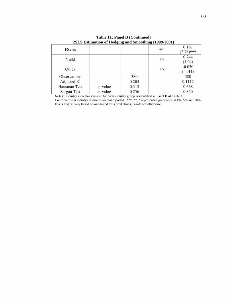
100

Table 11: Panel B (Continued) 2SLS Estimation of Hedging and Smoothing (1999-2001)

FSales +/- 0.167 (2.78)***

Yield +/- 0.744 (1.04)

Quick +/- -0.030 (-1.44)

Observations 380 380 Adjusted R2 0.204 0.1112

Hausman Test p-value 0.313 0.668 Sargan Test p-value 0.236 0.820

Notes: Industry indicator variable for each industry group is identified in Panel B of Table 1. Coefficients on industry dummies are not reported. ***, **, * represents significance at 1%, 5% and 10% levels respectively based on one-tailed tests predictions, two-tailed otherwise.

101

Table 12 Mean Volatility and Smoothing by Extent of Hedging (2000-2001)

Quintile Earnings Vol. Cash Flow Vol. Smoothing Non-User 1.089 2.819 1.659

1 2.175 2.339 2.209 2 1.133 2.266 2.097 3 0.899 2.633 1.783 4 0.883 2.707 1.883 5 1.910 1.727 2.343

Notes: Quintile 1 refers to the bottom 20% and quintile 5 refers to the top 20% in extent of derivative use measured using notional values. Includes all outliers.

102

Table 13: Panel A Effects of Hedge Accounting Treatment on Derivatives by Quintiles (2000-2001)

Independent Variables Predicted Sign Bottom 20% Coeff. (t-stat)

Top 20% Coeff. (t-stat)

Intercept +/- 0.034 (1.89)

1.279 (2.46)**

EVol + 0.000 (0.37)

-0.001 (-0.14)

CFVol + 0.001 (2.05)**

-0.032 (-1.47)*

Smooth - -0.000 (-0.38)

0.061 (1.67)*

After +/- 0.004 (0.84)

0.081 (0.46)

DNQ +/- -0.001 (-0.16)

-0.224 (-1.20)

Bdebt + 0.004 (1.07)

-0.117 (-1.95)*

B/M Ratio +/- -0.007 (-1.76)*

-0.078 (-0.92)

Analyst +/- -0.004 (-1.21)

0.047 (0.61)

Tax +/- -0.008 (-3.18)***

-0.137 (-1.80)*

Options +/- -0.002 (-1.44)

0.034 (1.06)

Size +/- 0.001 (0.62)

-0.130 (-2.56)**

Divers +/- 0.002 (0.68)

0.007 (0.11)

Libor +/- 0.002 (0.11)

1.534 (1.70)*

FX +/- -0.010 (-1.01)

-0.047 (-0.53)

PPI +/- 0.002 (0.52)

0.044 (0.46)

CFVol*After +/- -0.001 (-1.25)

0.071 (0.93)

CFVol*Term*After + 0.001 (0.37)

-0.036 (-0.47)

EVol*After +/- 0.000 (0.07)

-0.158 (-0.84)

EVol*Term*After + -0.002 (-0.39)

0.269 (1.37)*

Smooth*After +/- -0.000 (-0.06)

-0.047 (-1.16)

Smooth*Term*After + 0.001 (0.57)

-0.023 (-0.60)

Observations 60 65 Adjusted R2 0.065 0.063

103

Table 13: Panel B Effects of Transition Adjustment on Derivatives by Quintiles (2000-2001)

Independent Variables Predicted Sign Bottom 20% Coeff. (t-stat)

Top 20% Coeff. (t-stat)

Intercept +/- 0.043 (2.58)**

1.171 (2.17)**

EVol + 0.000 (0.50)

0.001 (0.12)

CFVol + 0.001 (2.47)***

-0.029 (-1.17)

Smooth - -0.001 (-0.67)

0.059 (1.44)*

After +/- 0.001 (0.13)

-0.002 (-0.01)

TA +/- 0.010 (1.12)

-0.213 (-1.17)

Bdebt + 0.003 (0.96)

-0.079 (-1.26)

B/M Ratio +/- -0.007 (-1.77)*

-0.091 (-0.94)

Analyst +/- -0.006 (-1.64)

0.087 (1.10)

Tax +/- -0.007 (-2.67)***

-0.085 (-1.32)

Options +/- -0.003 (-2.06)**

0.020 (0.57)

Size +/- 0.001 (0.72)

-0.125 (-2.72)***

Divers +/- 0.001 (0.64)

0.017 (0.24)

Libor +/- -0.017 (-0.63)

1.744 (1.90)*

FX +/- -0.006 (-0.68)

-0.053 (-0.70)

PPI +/- -0.002 (-0.42)

0.027 (0.38)

CFVol*After +/- -0.001 (-1.93)*

0.079 (0.43)

CFVol*Term*After + 0.010 (1.81)**

-0.059 (-0.31)

EVol*After +/- 0.000 (0.32)

-0.005 (-0.02)

EVol*Term*After + -0.012 (-1.14)

0.075 (0.22)

Smooth*After +/- 0.000 (0.48)

-0.084 (-1.60)*

Smooth*Term*After + -0.004 (-1.20)

0.103 (2.10)**

Observations 60 65 Adjusted R2 0.156 0.118

104

Table 13: Panel C Effects of Hedge Termination on Derivatives by Quintiles (2000-2001)

Independent Variables Predicted Sign Bottom 20% Coeff. (t-stat)

Top 20% Coeff. (t-stat)

Intercept +/- 0.037 (2.37)**

1.356 (2.89)***

EVol + 0.000 (0.04)

-0.004 (-0.99)

CFVol + 0.001 (1.91)**

-0.025 (-1.15)

Smooth - -0.000 (-0.36)

0.049 (1.30)*

After +/- 0.002 (0.48)

-0.116 (-1.17)

Term +/- -0.004 (-0.85)

-0.087 (0.75)

Bdebt + 0.004 (1.13)

-0.117 (-1.82)*

B/M Ratio +/- -0.007 (-1.86)*

-0.039 (-0.47)

Analyst +/- -0.006 (-1.31)

0.009 (0.15)

Tax +/- -0.008 (-2.93)***

-0.114 (-1.95)*

Options +/- -0.003 (-1.50)

0.023 (0.74)

Size +/- 0.002 (0.87)

-0.114 (-2.45)**

Divers +/- 0.001 (0.60)

-0.027 (-0.47)

Libor +/- 0.008 (0.33)

1.402 (1.69)*

FX +/- -0.010 (-0.96)

-0.016 (-0.15)

PPI +/- 0.003 (0.64)

-0.004 (-0.05)

CFVol*After +/- -0.001 (-1.12)

0.026 (0.97)

CFVol*Term*After + -0.001 (-0.46)

-0.214 (-4.65)***

EVol*After +/- 0.000 (0.24)

0.068 (1.06)

EVol*Term*After + 0022 (1.26)

-0.044 (-0.57)

Smooth*After +/- -0.000 (-0.01)

-0.058 (-1.36)

Smooth*Term*After + -0.001 (-0.37)

0.329 (8.11)***

Observations 60 65 Adjusted R2 0.086 0.189

105

Chapter 5

Summary and Conclusions

The purpose of this study was to investigate the effects of SFAS 133 on the use of

derivatives, cash flow volatility, earnings volatility, and income smoothing one year

before and after the implementation of the standard. I use data from the 2000-2001

period for a sample of 305 nonfinancial, nonregulated Fortune 500 firms and run a series

of probit and pooled cross-sectional regressions with dummy variables to determine if the

implementation of SFAS 133 had any significant effect on firm hedging activities,

volatility of earnings and cash flows, and income smoothing. I define and measure three

dependent variables, particularly the notional values of derivatives, as a proxy for

hedging, for the coefficient of variation as a measure of volatility, and for an income

smoothing ratio as a measure of earnings management. I regress these dependent

variables on a set of explanatory variables that proxy for the incentives to hedge,

including financial distress, underinvestment, managerial risk aversion, information

asymmetry, and taxes. I include dummy variables to proxy for SFAS 133 and interact

these variables with the volatility and smoothing variables. I then compare the difference

in the coefficients on the interaction terms after SFAS 133, relative to the coefficients

before SFAS 133 for derivative users and a control group of non-users and within groups

of derivative users. I also test the sensitivity of my results by extending the analysis over

a longer interval, two-years prior to and one-year after implementation of SFAS 133. In

addition, I specify a fixed-effects model and a simultaneous equation model as alternative

specifications to test the robustness of my results. Finally, I test the sensitivity of my

106

results by assessing the variation in volatility and smoothing by the level of hedging

among low (bottom 20%) and high (top 20%) derivative users.

The implementation of SFAS 133 had raised concerns about the potential impact

the standard could have on firm hedging activities. Chief among these concerns has been

an increase in earnings volatility and a reduction in the use of derivatives. On the other

hand, efficient market theory implies that there should be no direct economic

implications because the increase in earnings volatility which is induced by the standard

is simply a change in the method of accounting for derivatives and is therefore not a

change in the derivative's inherent economic risk. Consequently, cash flow volatility

should be unaffected. Overall, the results of this study show no significant differences in

earnings volatility, cash flow volatility, and income smoothing between derivative users

and non-users before and after the implementation of SFAS 133. I also find no evidence

of any significant decline in the use of derivatives after the implementation of SFAS 133.

Even though a number of sample firms terminated or discontinued the use of derivatives,

overall derivative use, as measured by notional value, has increased after the

implementation of the standard. Thus, the empirical evidence does not support the claims

of critics nor managers who were concerned that SFAS 133 would prevent firms in their

decision to use derivatives or reduce the amount of derivatives used.

In assessing the impact of SFAS 133 within groups of derivative users, I find no

evidence of any significant differences in the association between earnings volatility,

cash flow volatility, and income smoothing between firms that qualify for hedge

accounting treatment and firms that hold speculative derivatives before and after the

implementation of the standard. On the other hand, I find some evidence of the effect of

107

the transition adjustment on derivative users. Firms that report a transition adjustment

appear to have smoothed earnings to manage volatility. I also find significant differences

in the association between hedging and smoothing between firms that terminated

derivatives and other derivative users. The lower association between hedging and

earnings volatility and higher association between hedging and smoothing suggests that

firms that terminated derivatives also engaged in a higher level of income smoothing to

mitigate the volatility induced by the termination. This result from the fixed effects

model leads me to the conclusion that SFAS 133 may be driving the earnings

management decisions of managers, particularly among the largest derivative users. I

find there is a lower association between hedging and cash flow volatility and a higher

association between hedging and smoothing among the largest derivative users. These

extreme derivative users have the lowest earnings volatility and the highest level of

smoothing in the period after implementation compared to other users and to the year

before.

If earnings volatility is costly to firms, then my results provide some support for

the critics' assertions that managers may end up focusing more on minimizing earnings

volatility through earnings management or other tools and employing less effective

hedging strategies. The relative increase in the association between hedging and

smoothing in the period after implementation provides evidence that managers will

engage in a higher level of smoothing to manage volatility. Furthermore, my results also

suggest that firms with the largest derivative users may be the ones most concerned and

affected by the standard.

108

There is also evidence consistent with prior research (Pincus and Rajgopal 2002)

that the extent of hedging is a marginally significant determinant of the extent of

smoothing, while the extent of smoothing is an insignificant determinant of the extent of

hedging. This is in contrast to Barton's (2001) finding of a simultaneous relation between

hedging and smoothing. My results differ from prior research because it documents a

positive relation between hedging and smoothing, implying that derivatives and

smoothing are used in a complementary manner. If managers use derivatives to hedge or

speculate, then they are likely to engage in a higher level of smoothing to reduce hedge

ineffectiveness.

I find that the control variables that proxy for the incentives to hedge also support

the risk management theories in the decision to hedge. Consistent with prior research, the

factors that affect the decision to hedge are different from the factors that determine the

extent of hedging. However, with the exception of bank debt, these incentive control

variables, in general, do not provide consistent and conclusive evidence on the extent of

hedging. Bank debt is also negatively related to earnings volatility and cash flow

volatility, consistent with firms having incentives to smooth earnings to avoid covenant

violations.

Although I examine a large sample of Fortune 500 firms that are more likely to

use derivatives and be affected by the implementation of SFAS 133, my study is not

without its limitations. I do not rule out an endogeneity bias even though my results

show no endogeneity bias. Many sample firms had incomplete information, which

reduced the number of observations available for testing each empirical model.

Consequently, low power in my tests may preclude me from finding any significant

109

differences. Furthermore, my sample is limited to a small number of non-derivative

users, and prevents me from matching non-users with derivative users on the basis of

asset size and industry. My study is also biased toward large Fortune 500 firms, and

additionally, I cannot rule out measurement errors in my measures of exposure, notional

values, and the smoothing ratios.

The long-term effect of the standard is still an interesting issue and therefore,

should continue to be addressed in future research. This study may be improved by

increasing the sample size and observations by including more non-derivative users. This

study can also be extended by testing the effects of SFAS on volatility and smoothing

over a longer period after the implementation of the standard. Although there is still

much inconsistency in the disclosures of notional values and fair values by sample firms,

nevertheless, the use of notional values has been validated by prior research. Researchers

should consider testing these variables and selecting firms that provide full disclosures on

both notional and fair values. My weak findings or failure to document an empirical

relationship in many cases could also be attributed to my use of aggregated notional

values. Future research in this area should consider disaggregating notional values by

the risk hedged and the type of instrument used to further determine the impact of

Statement 133, if any, on volatility and income smoothing. Furthermore, this line of

research should also focus on specific industries such as service industries, where

evidence on hedging is lacking. Despite its limitations, my study is the first to provide

empirical evidence on the effects of SFAS 133 on the use of derivatives, volatility and

smoothing. It lays the groundwork for further research into one of the most controversial

accounting standards implemented by regulators.

110

References Allayannis, G., and E. Ofek. 2001. Exchange rate exposure, hedging and the use of foreign currency derivatives. Journal of International Money and Finance 20 (2): 273-296. Allayannis, G. and J. Weston. 2001. The use of foreign currency derivatives and firm market value. Review of Financial Studies 14 (1): 243-276 _______. 2003. Earnings volatility, cash volatility, and firm value. Working paper, Darden School of Business, University of Virginia. Association for Financial Professionals. 2002. The impact of FAS 133 on the risk management practices of end users of derivatives. (September), Bethesda, MD: AFP. Badrinath, S., G. Gay, and J. Kale. 1989. Patterns of institutional investment, prudence and the managerial ‘safety-net’ hypothesis. Journal of Risk and Insurance 56 (4): 605-629. Barnea, A., J. Ronen, and S. Sadan. 1976. Classicatory smoothing of income with extraordinary items. The Accounting Review 51 (1): 110-122. Barnes, R. 2001. Earnings volatility and market valuation: An empirical investigation. Working paper, London Business School, London, England. Barth, M., J. Elliott, and M. Finn. 1999. Market rewards associated with pattern of increasing earnings. Journal of Accounting Research 37 (2): 387-413. Barton, J. 2001. Does the use of financial derivatives affect earnings management decisions? The Accounting Review 76 (1): 1-26. Bartov, E., F. Gul, and J. Tsui. 2000. Discretionary-accrual models and audit qualifications. Journal of Accounting and Economics 30 (3): 421-452. Bayless, R. 2001. Financial reporting issues in 2001. Speech delivered at The Practising Law Institute, Washington, D.C., March 2. Beatty, A. 1998. Assessing the use of derivatives as part of a risk-management strategy. Journal of Accounting and Economics 26: 353-357 Beaver, W., P. Kettler, and M. Scholes. 1970. The association between market determined and accounting determined risk measures. The Accounting Review 45 (4): 650-682.

111

Berkman, H., and M. Bradbury. 1996. Empirical evidence on the corporate use of derivatives. Financial Management 25 (2): 5-13. Bodnar, G., G. Hayt, R. Marston, and C. Smithson. 1998. 1998 Wharton survey of financial risk management by US non-financial firms. Financial Management 27 (4): 70-91. Bowen, R., S. Rajgopal, and M. Venkatachalam. 2002. Accounting choice, corporate governance and firm performance. Working paper, University of Washington, Seattle, WA. Breeden, D., and S. Viswanathan. 1998. Why do firms hedge? An asymmetric information model. Working paper, Duke University, Durham, NC. Burgstahler, D., and I. Dichev. 1997. Earnings management to avoid earnings decreases and losses. Journal of Accounting and Economics 24 (1): 99-126. Collins, D. W., and P. Hribar. 2000. Errors in estimating accruals: Implications for empirical research. Working paper, University of Iowa, Iowa City, IA. DaDalt, P., G. Gay, and J. Nam. 2001. Asymmetric information and corporate derivative use. Working paper, Georgia State University, Atlanta, GA. Dechow, P., R. Sloan, and A. Sweeney. 1995. Detecting earnings management. The Accounting Review 70 (2): 193-225. DeFond, M., and J. Jiambalvo. 1994. Debt covenant violation and manipulation of accruals. Journal of Accounting and Economics 17 (1-2): 145-176. Degeorge, F., J. Patel, and R. Zeckhahser. 1999. Earnings management to exceed thresholds. Journal of Business 72 (1): 1-33. DeMarzo, P., and D. Duffie. 1995. Corporate incentives for hedging and hedge accounting. Review of Financial Studies 8 (3): 743-771. _______. 1991. Corporate financial hedging with proprietary information. Journal of Economic Theory 53 (April): 261-286. Dhaliwal, D. S., M. Frankel, and R. Trezevant. 1994. The taxable and book income motivation for a LIFO layer liquidation. Journal of Accounting Research 32 (2): 278-289. Dye, R. 1988. Earnings management in an overlapping generations model. Journal of Accounting Research 26 (2): 195-235.

112

Faulkender, M. 2002. Fixed versus floating: Corporate debt and interest rate risk management. Working paper, Northwestern University, Chicago, IL. Fields, T., T. Lys, and L. Vincent. 2001. Empirical research on accounting choice. Journal of Accounting and Economics 31 (1): 255-307. Financial Accounting Standards Board. 2001. Accounting for derivative instruments and hedging activities. Statement of Financial Accounting Standards Nos. 133, 137 and 138. Stamford, CT: FASB. Froot, K., D. Scharfstein, and J. Stein. 1983. Risk management: Coordinating corporate investment and financing policies. Journal of Finance 48 (5): 1629-1658. Gay, G., and J. Nam. 1998. The underinvestment problem and corporate derivative use. Financial Management 27 (4): 53-69. Geczy, C., B. Minton, and C. Schrand. 1997. Why firms use currency derivatives. Journal of Finance 52 (4): 1323-1354. Graham, J., and C. Smith. 1999. Tax incentives to hedge. Journal of Finance 54 (6): 2241-2262 Graham, J., and D. Rogers. 2002. Do firms hedge in response to tax incentives? Journal of Finance 57 (2): 815-839. Guay, W. 1999. The impact of derivatives on firm risk: An empirical examination of new derivative users. Journal of Accounting and Economics 26 (1-3): 319-351. Guay, W. and S. P. Kothari. 2001. How much do firms hedge with derivatives. Working paper, University of Pennsylvania, Philadelphia, PA. Guenther, D. 1994. Earnings management in response to corporate tax rate changes: Evidence from the 1986 Tax Reform Act. The Accounting Review 69 (1): 230- 243. Hand, J. 1989. Did firms undertake debt-equity swaps for an accounting paper profit or true financial gain? The Accounting Review 64 (4): 587-623. Haushalter, D. 2000. Financing policy, basis risk, and corporate hedging: Evidence from oil and gas producers. Journal of Finance 55 (1): 107-152. Hausman, J. 1978. Specification tests in econometrics. Econometrica 46 (6): 1251-1271. Healy, P., and J. Wahlen. 1999. A review of the earnings management literature and its implication for standard setting. Accounting Horizons 13 (4): 365-383

113

Healy, P. 1985. The effect of bonus schemes on accounting decisions. Journal of Accounting and Economics 7 (1-3): 85-107 Heckman, J. J. 1979. Sample selection bias as a specification error. Econometrica 47 (1): 153-162. Hentschel, L. and S. P. Kothari. 2001. Are corporations reducing or taking risks with derivatives? Journal of Financial and Quantitative Analysis 36 (1): 93-118 Holthausen, R., and R. Leftwich. 1983. The economic consequences of accounting choice: Implications of costly contracting and monitoring. Journal of Accounting and Economics 5 (2): 77-117. Howton, S. and S. Perfect. 1998. Currency and interest-rate derivative use in US firms. Financial Managemen 27 (4): 111-121. Hunt, A., S. Moyer, and T. Shevlin. 1997. Earnings volatility, earnings management, and equity value. Working paper, University of Washington, Seattle, WA. _______. 1996. Managing interacting accounting measures to meet multiple objectives: A study of LIFO firms. Journal of Accounting and Economics 21 (3): 339-374. Imhoff, G., and J. Thomas. 1988. Economic consequences of accounting standards: The lease disclosure rule change. Journal of Accounting and Economics 10 (4): 277- 310. Jones, J. 1991. Earnings management during import relief investigations. Journal of Accounting Research 29 (2): 193-228 Kasznik, R. 1999. On the association between voluntary disclosure and earnings management. Journal of Accounting Research 37 (1): 57-81. Lambert, R. 1984. Income smoothing as a rational equilibrium behavior. The Accounting Review 59 (4): 604-618. Leland, H. 1998. Agency costs, risk management and capital structure. Journal of Finance 53 (4): 1213-1243. Leuz, C., D. Nanda, and P. Wysocki. 2001. Investor protection and earnings management: An international comparison. Working paper, University of Pennsylvania, Philadelphia, PA. Lev, B. 1979. The impact of accounting regulations on the stock market. The case of oil and gas companies. The Accounting Review 54 (3): 485-503

114

Lundholm, R and L. Myers. 2002. Bringing the future forward: The effect of disclosure on the returns-earnings relation. Journal of Accounting Research, 40 (3): 809- 839. Lys, T. 1984. Mandated accounting changes and debt covenants: The case of oil and gas accounting. Journal of Accounting and Economics 6 (1): 39-65. McNichols, M. 2000. Research design issues in earnings management studies. Journal of Accounting and Public Policy 19 (4/5): 313-345. McNichols, M., and G. P. Wilson. 1988. Evidence of earnings management from the provision for bad debts. Journal of Accounting Research 26 (Supplement): 1-31. Mian, S. 1996. Evidence on corporate hedging policy. Journal of Financial and Quantitative Analysis 31 (3): 419-439. Minton, B. A., and C. Schrand. 1999. The impact of cash flow volatility on discretionary investment and the costs of debt and equity financing. Journal of Financial Economics 54 (3): 432-460. Modigliani, F., and M. H. Miller. 1958. The cost of capital, corporation finance and the theory of investment. American Economic Review 48 (3): 261-297. Myers, L., and D. Skinner. 1999. Earnings momentum and earnings management. Working paper, University of Michigan, Ann Arbor, MI. Myers, S. 1977. Determinants of corporate borrowing. Journal of Financial Economics 5 (2): 147-175. Nance, D., C. Smith, and C. Smithson. 1993. On the determinants of corporate hedging. Journal of Finance 48 (1): 267-284. Palepu, K. 1985. Diversification strategy, profit performance and the entropy measure. Strategic Management 6 (3): 239-255 Petersen, M. and S. Thiagarajan. 2000. Risk management and hedging: With and without derivatives. Financial Management 29: 5-30 Petroni, R. 1992. Optimistic reporting in the property casualty insurance industry. Journal of Accounting and Economics 15 (4): 485-508 Pincus, M., and S. Rajgopal. 2002. The interaction between accrual management and hedging: Evidence from oil and gas firms. The Accounting Review 77 (1): 127- 160.

115

Ronen, J., and S. Sadan. 1981. Smoothing income numbers: Objectives and implications. Reading, MA: Addison-Wesley Ross, M. P. 1997. Corporate hedging: What, why and how? Working paper, University of California, Berkeley, CA. Sargan, J. D. 1958. The estimation of economic relationships using instrumental variables. Econometrica 26: 393-415 Schipper, K. 1989. Commentary on earnings management. Accounting Horizons 3 (4): 91-102. Schrand, C., and H. Unal. 1998. Hedging and coordinated risk management: Evidence from thrift conversions. Journal of Finance 53 (3): 979-1013. Scott, W. 2003. Financial accounting theory. 3rd edition. Toronto, Canada: Prentice Hall. Sloan, R. 1996. Do stock prices fully reflect information in accruals and cash flows about future earnings? The Accounting Review 71 (3): 289-315. Smith, C., and R. Stulz. 1985. The determinants of firms' hedging policies. Journal of Financial and Quantitative Analysis 20 (4): 391-405. Stulz, R. 2003. Risk management and derivatives. Mason, Ohio: South-Western Publishing. _______. 1984. Optimal hedging policies. Journal of Financial and Quantitative Analysis 19 (2): 127-140 Subramanyam, K. R. 1996. The pricing of discretionary accruals. Journal of Accounting and Economics 22 (1-3): 249-281. Sweeney, A. P. 1994. Debt-covenant violations and managers’ accounting responses. Journal of Accounting and Economics 17 (3): 281-308. Teoh, S. H., I. Welch, and T. J. Wong. 1998a. Earnings management and the long-run market performance of initial public offerings. Journal of Finance 53 (6): 1935- 1974. _______. 1998b. Earnings management and the underperformance of seasoned equity offerings. Journal of Financial Economics 50 (1): 63-99. Teoh, S. H., I. Welch, and G. Rao. 1998c. Incentives and opportunities for earnings management in initial public offerings. Review of Financial Studies 3 (1-2): 175-208.

116

Trueman, B., and S. Titman. 1988. An explanation for accounting smoothing. Journal of Accounting Research 26 (Supplement): 127-139. Tufano, P. 1996. Who manages risk? An empirical examination of risk-management practices in the gold mining industry. Journal of Finance 51 (4): 1097-1137. Turner, L. 2001. The state of financial reporting today: An unfinished chapter III. Remarks delivered at the Glasser LegalWorks Third Annual SEC Disclosure & Accounting Conference, SanFrancisco, CA, June 21. Warner, J. 1977. Bankruptcy costs: Some evidence. Journal of Finance, 32 (1): 337- 348. Watts, R. L., and Zimmerman, J. L. (1990). Positive accounting theory: A ten year perspective. The Accounting Review 65 (1): 131-156. _______. 1986. Positive accounting theory. Englewood Cliffs, NJ: Prentice Hall. White, H. 1980. A heteroskedasticity consistent covariance matrix estimator and a direct test for heteroskedasticity. Econometrica 48 (4): 817-838 Wong, M. H. 2000. The association between SFAS No. 119 derivative disclosures and the foreign exchange risk exposure of manufacturing firms. Journal of Accounting Research 38 (2): 387-417 Wooldridge, J. 2000. Introductory Econometrics: A Modern Approach. Mason, Ohio: South-Western College Publishing. Zarowin, P. 2002. Does income smoothing make stock prices more informative? Working paper. New York University, New York, NY.

117

Appendix A Summary of SFAS 133 Requirements Designation and Recognition of Derivatives that Qualify for Hedge Accounting Treatment

1. Fair value hedge. A hedge of a recognized asset or liability or an unrecognized firm commitment. a. Gains and losses on the instrument and the offsetting losses and gains on

the hedged item are recognized in earnings in the same period

2. Cash flow hedge. A hedge of a recognized asset or liability or a forecasted transaction b. The effective portion of the gains and losses are recorded as a component

of Other Comprehensive Income (outside earnings) in Stockholder’s Equity and reclassified into earnings in the period when the transaction affects earnings

c. The ineffective portion of the gain or loss on the instrument is recognized in earnings.

3. Foreign currency hedge. A hedge of: a. An unrecognized firm commitment or a recognized asset or liability (fair

value hedge) b. An available-for-sale security (fair value hedge) c. A forecasted transaction, an unrecognized firm commitment, or the

forecasted functional currency cash flows of a recognized asset or liability (cash flow hedge)

d. A net investment in a foreign operation 1. For a fair value hedge, the gains and losses are recognized in

earnings in the same period. 2. For a cash flow hedge, the effective portion is recognized in

Other Comprehensive Income (outside earnings) in Stockholder’s Equity and reclassified into earnings in the period when the transaction affects earnings.

3. For a net investment in a foreign operation, the gain or loss will be recorded as part of the Cumulative Translation Adjustment (CTA) in Stockholder’s Equity.

Derivatives that do not qualify for Hedge Accounting Treatment

1. Trading and Speculative Derivatives

2. Hedges where the hedged item, instrument, financial risk do not qualify, or the hedge is not highly effective:

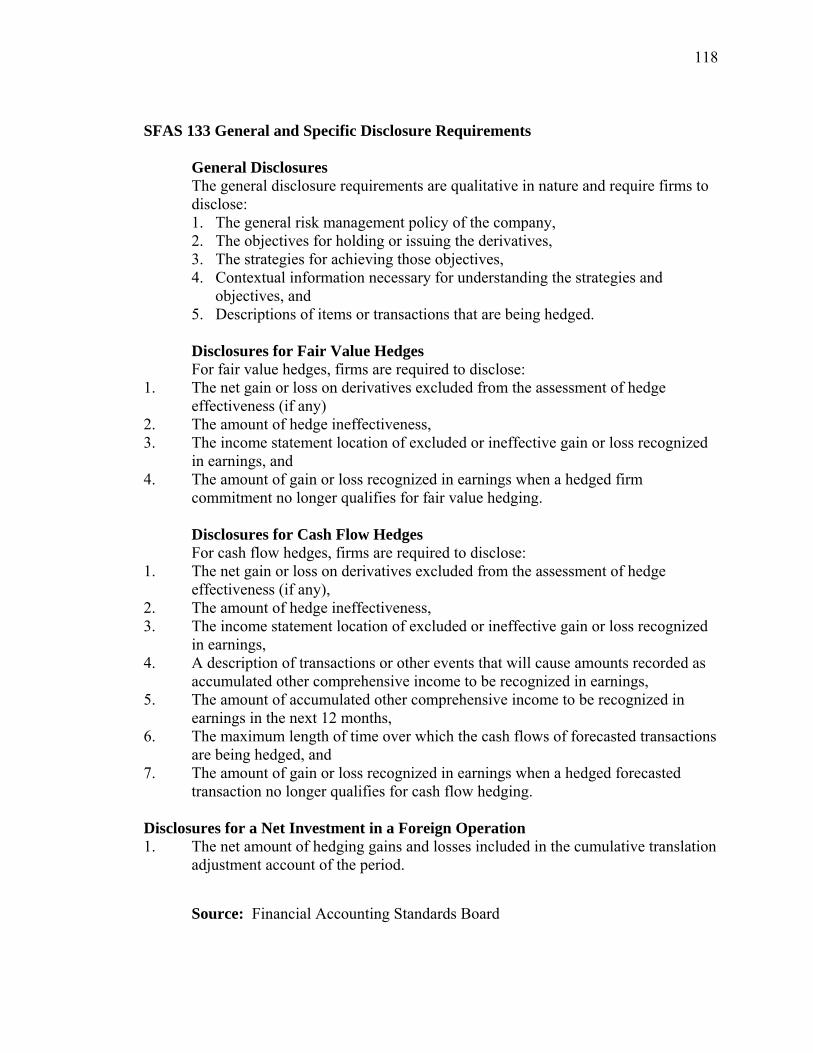
118

SFAS 133 General and Specific Disclosure Requirements General Disclosures The general disclosure requirements are qualitative in nature and require firms to

disclose: 1. The general risk management policy of the company, 2. The objectives for holding or issuing the derivatives, 3. The strategies for achieving those objectives, 4. Contextual information necessary for understanding the strategies and

objectives, and 5. Descriptions of items or transactions that are being hedged. Disclosures for Fair Value Hedges For fair value hedges, firms are required to disclose:

1. The net gain or loss on derivatives excluded from the assessment of hedge effectiveness (if any)

2. The amount of hedge ineffectiveness, 3. The income statement location of excluded or ineffective gain or loss recognized

in earnings, and 4. The amount of gain or loss recognized in earnings when a hedged firm

commitment no longer qualifies for fair value hedging. Disclosures for Cash Flow Hedges For cash flow hedges, firms are required to disclose:

1. The net gain or loss on derivatives excluded from the assessment of hedge effectiveness (if any),

2. The amount of hedge ineffectiveness, 3. The income statement location of excluded or ineffective gain or loss recognized

in earnings, 4. A description of transactions or other events that will cause amounts recorded as

accumulated other comprehensive income to be recognized in earnings, 5. The amount of accumulated other comprehensive income to be recognized in

earnings in the next 12 months, 6. The maximum length of time over which the cash flows of forecasted transactions

are being hedged, and 7. The amount of gain or loss recognized in earnings when a hedged forecasted

transaction no longer qualifies for cash flow hedging. Disclosures for a Net Investment in a Foreign Operation 1. The net amount of hedging gains and losses included in the cumulative translation

adjustment account of the period.

Source: Financial Accounting Standards Board

119

Appendix B

Maytag Corporation Annual 10-K Report, 2002: Selected Derivative Disclosures Market Risks Maytag is exposed to foreign currency exchange risk related to its transactions, assets and

liabilities denominated in foreign currencies. Foreign currency forward and option contracts are entered into to manage certain foreign exchange exposures. Maytag also is exposed to commodity price risk related to its purchase of selected commodities used in the manufacturing of its products. Commodity swap agreements are entered into reducing the effect of changing raw material prices for selected commodities.

Maytag also is exposed to interest rate risk in the portfolio of its debt. Maytag uses interest rate swap contracts to adjust the proportion of total debt that is subject to variable and fixed interest rates. The swaps involve the exchange of fixed and variable rate payments without exchanging the notional principal amount.

Non-Exchange Traded Contracts Accounted for at Fair Value The Company has a trading program of interest rate swaps that it marks to market each period.

The swap transactions involve the exchange of Canadian variable interest and fixed interest rate instruments. As of December 31, the Company had five swap transactions outstanding that mature on June 10, 2003 with a total notional amount of $53.8 million and $61 million as of December 31, 2002 and December 31, 2001, respectively. The fair value of the swap positions of $4.7 million at December 31, 2002 and $14.9 million at December 31, 2001 is reflected in Other noncurrent liabilities in the Consolidated Balance Sheets.

Notes to Consolidated Financial Statements Summary of Significant Accounting Policies Financial Instruments: The Company uses foreign exchange forward contracts to manage the

currency exchange risk related to sales denominated in foreign currencies. The Company uses commodity swap agreements to manage the risk related to changes in the

underlying material prices of component parts used in the manufacture of home and commercial appliances.

The Company has a trading program of interest rate swap contracts outstanding that are marked to

market each period. The Company uses interest rate swap contracts to adjust the proportion of total debt that is subject

to variable and fixed interest rates. The interest rate swap contracts are designated as fair value hedges. Financial Instruments The Company uses foreign currency exchange forward contracts to manage the currency exchange

risk related to sales denominated in foreign currencies. The counterparties to the contracts are high credit quality international financial institutions. Forward contracts used by the Company include contracts for the exchange of Canadian and Australian dollars to U.S. dollars to hedge the sale of appliances manufactured in the United States and sold to customers in Canada and Australia. The fair values of the contracts as of December 31, 2002 and 2001, which were reflected in Other current assets of the Consolidated Balance Sheets, were $0.1 million and $0.8 million, respectively. For 2002, 2001 and 2000, the gains and losses from these contracts were not significant. As of December 31, 2002 and 2001, the Company had open

120

foreign currency forward contracts, all with maturities of less than twelve months, in the amount of U.S. $32.9 million and U.S. $50.4 million, respectively.

The Company uses commodity swap agreements to manage the risk related to changes in the

underlying material prices of component parts used in the manufacture of home and commercial appliances. The fair value of the contracts as of December 31, 2002, and 2001, which were reflected in Other current assets of the Consolidated Balance Sheets, were $0.5 million and $0.6 million, respectively. For 2002, 2001 and 2000, $0.5 million of gains, $0.9 million of losses, and $5.7 million of gains were recognized from these contracts, respectively. As of December 31, 2002 and 2001, the Company had open commodity swap contracts in the amount of U.S. $6 million and U.S. $10.5 million, respectively. Open contracts as of December 31, 2002 have maturities ranging from one month to two years.

The Company has a trading program of interest rate swaps that it marks to market each period.

The swap transactions involve the exchange of Canadian variable interest and fixed interest rate instruments. As of December 31, 2002, the Company had five swap transactions outstanding that mature on June 10, 2003 with a total notional amount of $53.8 million and $61 million as of December 31, 2002 and December 31, 2001, respectively. The fair value of the swap positions of $4.7 million at December 31, 2002 and $14.9 million at December 31, 2001 is reflected in Other noncurrent liabilities in the Consolidated Balance Sheets.

The Company uses interest rate swap contracts to adjust the proportion of total debt that is subject

to variable and fixed interest rates. To manage associated cost of this debt, the Company enters into interest rate swaps, in which the Company agrees to exchange, at specified intervals, the difference between interest amounts calculated by reference to an agreed upon notional principal amount. These swap contracts are used to hedge the fair value of certain medium term notes. The contracts are a perfect hedge as their terms, interest rates and payment dates exactly match the underlying debt. At December 31, 2002 and 2001, the Company had outstanding interest rate swap agreements with notional amounts totaling $250 million. Under these agreements, the Company receives weighted average fixed interest rates of 7.32 percent and pays floating interest rates based on LIBOR rates plus an agreed upon spread, or a weighted average interest rate of 5.63 percent, as of December 31, 2002. Maytag had interest rate swaps designated as fair value hedges of underlying fixed rate debt obligations with a fair market value as of December 31, 2002 and December 31, 2001 of $9.3 million and $10.9 million, respectively.

The fair values of interest rate swaps, foreign currency contracts, commodity swaps, forward stock

purchase contracts and put option contracts were estimated based on amounts the Company would pay to terminate the contracts at the reporting date.

The carrying amounts and fair values of the Company’s financial instruments, consisted of the

following:

(in thousands) Dec 31, 2002 Dec 31, 2001 Carrying Value Fair Value Carrying Value Fair Value

Interest rate swaps - trading (4,703) (4,703) (14,876) (14,876) Interest rate swaps – non-trading 9,257 9,257 10,949 10,949 Foreign currency contracts 90 90 831 831 Commodity swap contracts 531

Source: Maytag Annual 10-K Report

121

Appendix C Definition of Variables*

Construct Proxy Variable Total Notional Value of Derivatives

Aggregate total notional value of derivatives outstanding for each firm at year-end/Book value of assets at end of year. Annual 10-K report Deriv

Earnings Volatility

Coefficient of Variation measured as firm i’s standard deviation of quarterly earnings firm before extraordinary items/Absolute value of mean quarterly earnings before extraordinary items. (σ #76/|µ #76|)

EVol

Cash Flow Volatility

Coefficient of Variation measured as firm i’s standard deviation of quarterly operating cash flows/Absolute value of mean quarterly cash flows. (σ #108/|µ #108|)

CFVol

Smoothing Ratio

Ratio measured as the standard deviation of firm i’s quarterly cash flows/standard deviation of firm i’s quarterly income before extraordinary items and scaled by total assets at end of previous quarter. (#108/#8)/#44

Smooth

Smoothing Ratio

Ratio measured as the standard deviation of firm i’s quarterly income before discretionary accruals and extraordinary items in quarter t/standard deviation of firm i’s quarterly income before extraordinary items and scaled by total assets at end of previous quarter. Income before Discretionary Accruals = Cash Flow from Operations + Non-Discretionary Accruals. ((#108 + Non-Discretionary Accruals)/(#76))/#44

Smooth1

Bank Debt Equals 1 if has outstanding bank debt in yeat t; 0 otherwise BDebt Growth Opportunities

Book value of equity/Market value of equity of firm i at fiscal t year-end. (#60)/(#199 * #25)

B/M Ratio

Info. Asymmetry Number of analysts following firm i in year t. I/B/E/S Database Analyst

Income Taxes Dummy variable that equals 1 if firm i is profitable (Income before Extraordinary items>0) in year t and have NOL carry-forward at fiscal t year-end; otherwise 0. Compustat #18 and #52

Tax

Managerial Ownership

Logarithm of the total number of CEO stock options outstanding at end of fiscal year, Compustat Execucomp Options

Firm Size Log of book value of assets of firm i in year t (#6) Size Inverse Mills Ratio

Ratio between the standard normal PDF and the standard normal CDF. Computed for each firm using the binomial Probit model Mills

Industry Effect Dummy variable that equals 1 indicating membership in each 2-digit SIC group; otherwise 0 Industry

SFAS 133 1= After implementation of SFAS 133; 0 otherwise After Derivative User 1= Derivative user; 0 otherwise User Hedge Accounting Treatment

1= Firms do not qualify for hedge accounting; 0 otherwise DNQ

Transition Adjustment 1= Firm disclosing transition adjustment; 0 otherwise TA

Derivative Termination 1= Firm terminating derivatives in year t; 0 otherwise Term

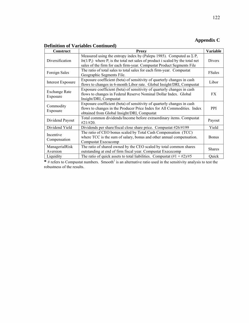
122

Appendix C Definition of Variables Continued)

Construct Proxy Variable

Diversification Measured using the entropy index by (Palepu 1985). Computed as Σ Pi ln(1/Pi) where Pi is the total net sales of product i scaled by the total net sales of the firm for each firm-year. Compustat Product Segments File

Divers

Foreign Sales The ratio of total sales to total sales for each firm-year. Compustat Geographic Segments File. FSales

Interest Exposure Exposure coefficient (beta) of sensitivity of quarterly changes in cash flows to changes in 6-month Libor rate. Global Insight/DRI, Compustat Libor

Exchange Rate Exposure

Exposure coefficient (beta) of sensitivity of quarterly changes in cash flows to changes in Federal Reserve Nominal Dollar Index. Global Insight/DRI, Compustat

FX

Commodity Exposure

Exposure coefficient (beta) of sensitivity of quarterly changes in cash flows to changes in the Producer Price Index for All Commodities. Index obtained from Global Insight/DRI, Compustat

PPI

Dividend Payout Total common dividends/Income before extraordinary items. Compustat #21/#20. Payout

Dividend Yield Dividends per share/fiscal close share price. Compustat #26/#199 Yield

Incentive Compensation

The ratio of CEO bonus scaled by Total Cash Compensation (TCC) where TCC is the sum of salary, bonus and other annual compensation. Compustat Execucomp

Bonus

ManagerialRisk Aversion

The ratio of shared owned by the CEO scaled by total common shares outstanding at end of firm fiscal year. Compustat Exececomp Shares

Liquidity The ratio of quick assets to total liabilities. Compustat (#1 + #2)/#5 Quick * # refers to Compustat numbers. Smooth1 is an alternative ratio used in the sensitivity analysis to test the robustness of the results.

123

Appendix D Notional & Fair Value Disclosures of 30 Excluded Firms X – indicates that firm has no disclosure of notional or fair value in period

before/after adoption of SFAS 133 in June 2000. NV = Notional Value; FV = Fair Value

TIC CoName NV before SFAS 133

NV after SFAS 133

FV before SFAS 133

FV after SFAS 133

A Agilent Tech. Inc X X X X ADM Archer-Daniels X X X X AVT Avnet Inc. X X X X NOC Northrop Grumman X X X X PH Parker-Hannifin X X X X NWAC Northwest Airlines X X X X SBUX Starbucks X X X X SGR Shaw Group X X X X BA Boeing Co. X X X JNJ Johnson & Johnson X X X MSFT Microsoft Corp. X X X EMN Eastman Chemical X X X SSOC Smurfit-Stone X X X HD Home Depot X X X ASH Ashland Inc. X X AZO Autozone Inc. X X DRI Darden Restaurants X X HCA HCA Inc. X X IB Interstate Bakeries X X IPG Interpublic Group X X LMT Lockheed Martin X X MHK Mohawk Industries X X PAS PepsiAmericas X X AMAT Applied Materials X X F Ford Motor Co. X X UCL Unocal Corp. X X UIS Unisys Corp. X X MMM 3M Co. X X XOM Exxon Mobil X X VFC VF Corp. X X Totals 21 19 25 17

Source: SEC 10-K filings

124

Appendix E Selective Disclosures of Non-Qualifying Derivatives of Fortune 500 Firms " In some situations, the corporation has chosen not to designate certain immaterial derivatives

used for hedging economic exposure as hedges for accounting purposes due to the excessive administrative effort that would be required to account for these items as hedging transactions" (Exxon-Mobil 2001 Form 10-K: Notes to Consolidated Financial Statements, p. 38 )

"Valero uses derivative commodity instruments (swaps, futures, and options) to manage its

exposure to: price volatility on a portion of its refined product inventories and on certain forecasted feedstock and refined product purchases that are not designated as either fair values or cash flow hedges. In addition, Valero uses derivative commodity instruments for trading purposes based on its fundamental and technical analysis of market conditions." (Valero Energy Corporation 2002 Form 10-K: Notes to Consolidated Financial Statements, No. 17, p. 88)

"Our foreign currency risk management objective is to protect our earnings and cash flows from

the adverse impact of exchange rate changes. Foreign exchange risk is managed by using foreign currency forwards, options, and swap contracts, to hedge inter-company loans, trade receivables and payables. We have elected not to designate our foreign currency contracts as hedging instruments, and they are therefore marked to market with changes in their value recorded in the income statement in each period." (Tech Data Corporation 2002 Form 10-K: Item 7a, p.24)

"As a policy, the company does not engage in speculative or leveraged transactions, nor does the

company hold or issue financial instruments for trading purposes. The company enters into certain derivative contracts in accordance with its risk management strategy that do not meet the criteria for hedge accounting. Although these derivatives do not qualify as hedges, they have the economic impact of largely mitigating foreign currency, commodity price or interest rate exposures. These derivative instruments are accounted for on a full mark to market basis through current earnings even though they were not acquired for trading purposes." (Heinz H. J. Co Inc. 2002 10-K: Notes to Consolidated Financial Statements, p. 37,54)

"The company uses forward contracts and cross-currency swap agreements to hedge earnings from

the effects of fluctuations in currency exchange rates relating to certain of the company's inter-company and third-party receivables and payables denominated in a foreign currency. These derivative instruments are not formally designated as hedges, and the change in the fair value of these instruments, which substantially offsets the changes in the book value of the hedged items, is recorded directly to earnings. (paragraph omitted). In conjunction with the company's rebalancing of its debt portfolio and in anticipation of the adoption of SFAS 133, certain of such contracts (cross currency swaps and equity puts and calls)were terminated in 2000 and a gain was recognized in other income." (Baxter International 2000 & 2001 10-K: Notes to Consolidated Financial Statements, p. 41, 51)

"Due to the complex nature of risks we attempt to hedge, our commodity financial instruments

have generally not qualified as effective hedges under SFAS 133. Even though these financial instruments may not qualify for hedge accounting treatment under SFAS 133, we view such contracts as hedges since this was the intent when we entered into such positions. Upon entering into such positions, our expectation is that the economic performance of these instruments will mitigate (or offset) commodity risk being addressed." (Enterprise products Partner 2002 Form 10-K: Item 7a, p. 56)

Vita Amrik Singh

EDUCATION

Ph.D, Hotel Restaurant & Institutional Mgt., The Pennsylvania State University, 2004 M.S., Hotel Administration, University of Nevada, Las Vegas,1994 B.S., Recreation & Leisure, University of Utah, Salt Lake City, Utah, 1990

EXPERIENCE

Instructor, School of Hotel Restaurant and Recreation Management, The Pennsylvania State University, University Park, Pennsylvania, 2001-2004

Clinical Instructor and Coordinator of Hospitality Program, Department of Parks, Recreation and Tourism, University of Utah, Salt Lake City, Utah, 1995-1999.

Assistant Banquet Service Manager, The Regent Singapore, Four Seasons Hotels & Resorts, Singapore 1994-1995

HONORS AND AWARDS

Grace L. Henderson Scholarship Award for Outstanding Graduate Student, College of Health & Human Development, The Pennsylvania State University, 2002

Outstanding Graduate Research Award for Best Thesis, College of Hotel Administration, University of Nevada, Las Vegas, 1995

Best Paper Award, Council on Hotel, Restaurant and Institutional Education (CHRIE) Annual Conference, Palm Springs, 1994.

Bob Brown Memorial Scholarship Award for Outstanding Graduate Student, College of Hotel Administration, University of Nevada, Las Vegas, 1994

Outstanding Undergraduate Student, Department of Recreation and Leisure, University of Utah, 1990.

Undergraduate Merit Scholarship, Department of Recreation and Leisure, University of Utah, 1989.

MEMBERSHIPS

Member of International Council on Hotel, Restaurant & Institutional Education (I-CHRIE) Member of American Accounting Association