THE EFFECTS OF TEST DRIVEN DEVELOPMENT ON SOFTWARE PRODUCTIVITY AND SOFTWARE QUALITY

A THESIS SUBMITTED TO THE GRADUATE SCHOOL OF NATURAL AND APPLIED SCIENCES

OF MIDDLE EAST TECHNICAL UNIVERSITY

BY

CUMHUR ÜNLÜ

IN PARTIAL FULFILLMENT OF THE REQUIREMENTS FOR

THE DEGREE OF MASTER OF SCIENCE IN

ELECTRICAL AND ELECTRONICS ENGINEERING

SEPTEMBER 2008

Approval of the thesis:

THE EFFECTS OF TEST DRIVEN DEVELOPMENT ON

SOFTWARE PRODUCTIVITY AND SOFTWARE QUALITY

submitted by CUMHUR ÜNLÜ in partial fulfillment of the requirement for the degree of Master of Science in Electrical and Electronics Engineering Department, Middle East Technical University by, Prof. Dr. Canan Özgen Dean, Graduate School of Natural and Applied Sciences Prof. Dr. Đsmet Erkmen Head of Department, Electrical and Electronics Engineering Prof. Dr. Semih Bilgen Supervisor, Electrical and Electronics Engineering Examining Committee Members: Prof. Dr. Uğur Halıcı Electrical and Electronics Engineering Dept., METU Prof. Dr. Semih Bilgen Electrical and Electronics Engineering Dept., METU Asst. Prof. Dr. Cüneyt Bazlamaccı Electrical and Electronics Engineering Dept., METU Asst. Prof. Dr. Đlkay Ulusoy Electrical and Electronics Engineering Dept., METU Hakan Öztarak (M.Sc.) Test Engineering Department, ASELSAN A.Ş.

Date:

iii

LAGIARISM

LAGIARISM

I hereby declare that all information in this document has been obtained and presented in accordance with academic rules and ethical conduct. I also declare that, as required by these rules and conduct, I have fully cited and referenced all material and results that are not original to this work.

Name, Last name: CUMHUR ÜNLÜ

Signature :

iv

ABSTRACT

THE EFFECTS OF TEST DRIVEN DEVELOPMENT ON

SOFTWARE PRODUCTIVITY AND SOFTWARE QUALITY

ÜNLÜ, Cumhur

M. Sc., Department of Electrical and Electronics Engineering

Supervisor: Prof. Dr. Semih BĐLGEN

September 2008, 84 pages

In the 1990s, software projects became larger in size and more complicated in

structure. The traditional development processes were not able to answer the

needs of these growing projects. Comprehensive documentation in traditional

methodologies made processes slow and discouraged the developers. Testing,

after all code is written, was time consuming, too costly and made error

correction and debugging much harder. Fixing the code at the end of the project

also affects the internal quality of the software. Agile software development

processes evolved to bring quick solutions to these existing problems of the

projects. Test Driven Development (TDD) is a technique, used in many agile

methodologies, that suggests minimizing documentation, writing automated tests

before implementing the code and frequently run tests to get immediate feedback.

The aim is to increase software productivity by shortening error correction

duration and increase software quality by providing rapid feedback to the

developer. In this thesis work, a software project is developed with TDD and

compared with a control project developed using traditional development

techniques in terms of software productivity and software quality. In addition,

v

TDD project is compared with an early work in terms of product quality. The

benefits and the challenges of TDD are also investigated during the whole

process.

Keywords: Agile Software Development, Test Driven Development, Software

Productivity, Software Quality.

vi

ÖZ

SINAMAYA DAYALI GELĐŞTĐRMENĐN YAZILIM ÜRETKENLĐĞĐ

VE YAZILIM NĐTELĐĞĐNE ETKĐLERĐ

ÜNLÜ, Cumhur

Yüksek Lisans, Elektrik ve Elektronik Mühendisliği Bölümü

Tez Yöneticisi: Prof. Dr. Semih BĐLGEN

Eylül 2008, 84 Sayfa

1990’larda, yazılım projeleri boyutça daha büyük ve yapıca daha karmaşık bir

hale geldi. Geleneksel geliştirme süreçleri bu büyüyen projelerin ihtiyaçlarına

cevap veremedi. Geleneksel metotlarda yapılan kapsamlı dokümantasyon,

süreçleri yavaşlatıyor ve yazılım geliştiricileri isteksizleştiriyordu. Kod

yazımından sonra testlerin yapılması fazla zaman alıyordu, çok masraflıydı ve

hata düzeltme ile hata ayıklamayı zorlaştırıyordu. Kodun projenin sonunda

düzeltilmesi de yazılımın içsel niteliğini etkiliyordu. Çevik yazılım geliştirme

süreçleri bilinen bu problemlere hızlı çözümler getirebilmek için geliştirildi.

Sınamaya Dayalı Geliştirme (SDG) birçok çevik metotta kullanılan,

dokümantasyonun azaltılmasını, kod yazılmadan önce otomatik testlerin

yazılmasını ve hızlı geri besleme alınması için testlerin sıkça koşturulmasını

öneren bir tekniktir. Amaç, hata düzeltme zamanını kısaltarak yazılım

üretkenliğini ve yazılım geliştiriciye hızlı geri beslemeler sağlayarak yazılım

niteliğini arttırmaktır. Bu tezde, SDG tekniği ile bir proje geliştirildi ve geleneksel

geliştirme tekniği ile geliştirilen bir kontrol projesi ile yazılım üretkenliği ve

yazılım niteliği açısında karşılaştırıldı. Buna ek olarak, SDG projesi, daha önce

vii

geliştirilmiş olan bir projeyle ürün niteliği açısından karşılaştırıldı. SDG

uygulanmasının yararları ve zorlukları da çalışma boyunca incelendi.

Anahtar Kelimeler: Sınamaya Dayalı Geliştirme, Çevik Yazılım Geliştirme,

Yazılım Üretkenliği, Yazılım Niteliği

viii

To My Parents and To My Brother

ix

ACKNOWLEDGMENTS

I would like to express my sincere gratitude to my supervisor Prof. Dr. Semih

Bilgen for his understanding, patience and supervision throughout this thesis. This

thesis would not have been completed without his realistic, encouraging and

constructive guidance.

I would like to express my appreciation to ASELSAN Inc. for providing tools and

other facilities throughout this study.

I would like to thank to all my friends and colleagues for their understanding and

continuous support during my thesis. Special thanks to Oğuz Kurt for his valuable

comments, suggestions and encouragement.

Finally, I would like to thank my family - my brother, my mom and my dad - for

their love, trust, understanding and every kind of support not only throughout my

thesis but also throughout my life.

x

TABLE OF CONTENTS

ABSTRACT ...........................................................................................................iv

ÖZ…………...........................................................................................................vi

ACKNOWLEDGMENTS......................................................................................ix

TABLE OF CONTENTS ........................................................................................x

LIST OF TABLES ............................................................................................... xii

LIST OF FIGURES............................................................................................. xiii

LIST OF ABBREVIATIONS ..............................................................................xiv

CHAPTER

1. INTRODUCTION..........................................................................................1

2. TEST DRIVEN DEVELOPMENT................................................................4

2.1 AGILE SOFTWARE DEVELOPMENT................................................ 4

2.2 INTRODUCTION TO TDD ................................................................... 6

2.3 BENEFITS OF TDD............................................................................... 8

2.4 CHALLENGES OF TDD ....................................................................... 9

2.5 SOFTWARE METRICS ....................................................................... 10

2.5.1 SOFTWARE PRODUCTIVITY METRICS................................. 12

2.5.1.1 LINES OF CODE (LOC) .............................................................. 12

2.5.1.2 FUNCTION POINTS (FP)............................................................ 13

2.5.1.3 DOCUMENTATION PAGES ...................................................... 18

2.5.2 SOFTWARE QUALITY METRICS ............................................ 19

2.6 THE EFFECTS OF TDD ON SOFTWARE METRICS....................... 23

3. ASSESSMENT OF THE EFFECTS OF TDD.............................................28

3.1 EXPERIMENTAL DESIGN................................................................. 28

3.2 EXPERIMENT RESULTS ................................................................... 30

3.2.1 PROJECT A – RESULTS OF THE TDD PROJECT................... 30

3.2.2 PROJECT B – RESULTS OF THE TEST-LAST PROJECT ...... 36

3.2.3 PROJECT C – EARLY WORK.................................................... 42

4. DISCUSSION AND CONCLUSION..........................................................45

4.1 RESULTS COMPARISON AND DISCUSSION ................................ 45

xi

4.2 CONCLUSION ..................................................................................... 51

REFERENCES...................................................................................................... 53

APPENDICES

A.SOFTWARE METRICS ................................................................................... 59

B.SOFTWARE SIZE MEASUREMENT METHODS [30]................................. 62

C.OVERALL REPRESENTATION OF PROCESS METRICS EVALUATED

FOR PROJECT B............................................................................................... 63

D.LRF SIMULATOR – PROJECT B................................................................... 65

E.FUNCTION POINTS CALCULATION DETAILS FOR PROJECT B .......... 69

F.OVERALL REPRESENTATION OF PROCESS METRICS EVALUATED

FOR PROJECT A .............................................................................................. 74

G.STREELETS SIMULATOR – PROJECT A .................................................... 76

H. FUNCTION POINTS CALCULATION DETAILS FOR PROJECT A ......... 79

xii

LIST OF TABLES

Table 2.1 Internal Quality Metrics with Warnings [12]………………..…….. 26

Table 2.2 Related Works……………………………………………………... 26

Table 3.1 Overall Quality Metrics of Project A ……………...………...……. 35

Table 3.2 Minimum and Maximum Values for the Product Metrics Evaluated

for Project A …………………………...…...………………….….. 35

Table 3.3 Overall Quality Metrics of Project B ……………...………...……. 41

Table 3.4 Minimum and Maximum Values for the Product Metrics Evaluated

for Project B ………………………………….…...………...…….. 41

Table 3.5 Overall Quality Metrics of Project C ……………...………...……. 43

Table 3.6 Minimum and Maximum Values for the Product Metrics Evaluated

for Project C ………………………………….…...………...…….. 44

Table 4.1 Effort Percentages of Projects A and B…………………………… 48

Table 4.2 Overall Quality Metrics of Projects A, B and C…………………... 49

Table A.1 Software Product Metrics [18]…………………………………….. 59

Table A.2 Software Process Metrics [26]…………………………………….. 61

Table B Software Size Measurement Methods [30]......……………………. 62

Table C Project B Process Metrics....………………………………………. 63

Table E FP Tables of all Versions for Project B……………………………. 69

Table F Project A Process Metrics.......……………………………………...74

Table H FP Tables of all Versions for Project A……………………………. 79

xiii

LIST OF FIGURES

Figure 2.1 TDD Cycle [4]…..…………………………...……………………7

Figure 2.2 IFPUG Function Point Analysis Attributes [22]…………………15

Figure 2.3 Flow Chart Example of a Function [24]…......…………………..20

Figure 2.4 Defect Density Measurement Process[39]……………………….25

Figure 3.1 LOCs versus Staff-Hours for Project A……………………….....31

Figure 3.2 Function Points versus Staff-Hours for Project A.….…………...32

Figure 3.3 Defects Found versus Staff-Hours for Project A...…...………….32

Figure 3.4 Defects Found versus Line of Codes for Project A.……………..33

Figure 3.5 Effort Percentage Graph for Project A...……………...……….…34

Figure 3.6 Waterfall Method…...………………………………...……….…36

Figure 3.7 LOCs versus Staff-Hours for Project B……………………….....37

Figure 3.8 Function Points versus Staff-Hours for Project B..….…………...38

Figure 3.9 Defects Found versus Staff-Hours for Project B………………...39

Figure 3.10 Defects Found versus Line of Codes for Project B. ……………..39

Figure 3.11 Effort Percentage Graph for Project A...……………...……….…40

Figure 4.1 LOCs versus Staff-Hours for Project A and B…..…………….…45

Figure 4.2 Function Points versus Staff-Hours for Project A and B.………..46

Figure 4.3 Defects Found versus Staff-Hours for Project A and B………….47

Figure 4.4 Defects Found versus Line of Codes for Project A and B……….47

Figure D GUI of the LRF…………………………………………………..65

Figure G GUI of the STRELETS…………………………………………..76

xiv

LIST OF ABBREVIATIONS

AFP Adjusted Function Points

ARCHI-DIM Architecturel Dimensions Based FSM

ASD Adaptive Software Development

AUP Agile Unified Process

BFC Base Functional Component

CBO Coupling Between Objects

CC Cyclomatic Complexity

CMMI Capability Maturity Model Integration

COSMIC Common Software Measurement International Consortium

DIT Depth of Inheritance Tree

DSDM Dynamic Systems Development Method

EI External Input

EIF External Interface File

EO External Output

EQ External Inquiry

FDD Feature Driven Development

FFP Full Function Points

FP Function Points

FPA Function Point Analysis

FPC Function Point Count

FSM Functional Size Measurement

FUR Functional User Requirements

GUI Graphical User Interface

IBM International Business Machines Corporation

IF Information Flow

IFPUG International Function Point Users Group

xv

ILF Internal Logical File

ISO International Standards Organization

LCOM Lack of Cohesion Of Methods

LOC Lines Of Code

METU Middle East Technical University

MSN Microsoft Network

NESMA The Netherlands Software Metrics Users Association

NOC Number Of Children

OO Object Oriented

RFC Response For a Class

SDG Sınamaya Dayalı Geliştirme

TDD Test Driven Development

UFP Unadjusted Function Points

VAF Value Adjustment Factor

WMC Weighted Methods per Class

XP Extreme Programming

1

CHAPTER 1

INTRODUCTION

In the 1990s, people started to figure out the weaknesses of the traditional

software development processes [27]. The requirements need to be fixed during

the process, but it is too costly to make changes after a certain point in traditional

methodologies. Furthermore, these methods resist altering requirements, because

changes lead to delays and delays break down the predicted schedule. Moreover,

the aim in a project is that the outcome will not depend on the individuals but in

reality, the project failures or successes heavily depend on the individuals

involved. Consequently, new methodologies, having common values such as

responding to change, interactions between individuals, working software and

customer collaboration, were developed and they are all grouped as Agile

Methodologies.

In many agile software development processes, Test Driven Development (TDD)

technique is used. TDD is a style of development and can be summarized in five

steps: Quickly add a test; run all tests and see the new one fail; write the

necessary code; run all tests and see the new one pass; refactor code [2, 3].

Minute by minute testing in TDD provides instant feedback to the developer [6].

The features are divided into manageable tasks as a result of the iterative

development [5]. Moreover, low level designs are made in each iteration, in the

writing tests phase. Easy regression tests, achieved by automated tests, can be

considered as another benefit of TDD.

2

On the other hand, there are some challenges of TDD. In the software

development projects including database, network, embedded software and

graphical user interface, it is mentioned that applying TDD may be not possible or

useless [7, 8, 9]. In addition, lack of familiarity of the developers to TDD and

insufficient tool support for the automation of tests can lead to serious delays in

the project timeline.

In the literature, there is a debate about the effects of TDD on the software

development process. There are some studies in industry and academy indicating

that TDD leads to an increase in developer’s productivity [5, 10] and software

quality [4, 39]. There are also opposing ideas and studies [1, 4, 12]. These studies

claim that TDD has no significant effect on software quality and that it also

decreases the developers’ productivity.

In this thesis study, we perform a case study to assess how TDD affects software

productivity and software quality. To evaluate the effects of TDD, two software

projects developed at Aselsan A.Ş., are considered. One of them is the control

project and is developed using traditional Test-Last development technique; the

second one is a similar project and is implemented using TDD. Software product

metrics that are indicators of quality, and process metrics that measure

productivity [13] are calculated for both projects and the evaluation results are

compared to determine the differences between them in terms of productivity and

quality.

The projects include graphical user interface and network applications. Besides

assessing the effects of TDD, challenges of using TDD in a network and GUI

application are also examined in the scope of this thesis.

In addition to comparison of the above mentioned projects, the TDD project is

compared with an early work performed at Aselsan A.Ş in terms of product

quality. This early work was developed using Test-Last development technique. It

3

should be noted that the aim of the study is to present a case-based contribution to

the arguments on the merits of TDD, rather than establishing a definitive

conclusion, which would be much above and beyond the scope of this thesis.

The outline of the thesis is organized as follows: Chapter 2 provides background

information about test driven development, a literature survey about software

productivity and quality metrics and results available in the literature related with

the subject of this thesis. Chapter 3 presents the overview and the results of the

TDD project, Test-Last project and the early work. Finally in Chapter 4 the

obtained results are compared and discussed; the overall development process is

summarized and the study is concluded.

4

CHAPTER 2

TEST DRIVEN DEVELOPMENT

In this chapter, first, an overview of the literature on the subject of agile software

development and test driven development (TDD) is given. Then, some TDD

related studies are examined and possible benefits and some challenges of TDD

are reviewed. In this context, the importance of software metrics is noted, and the

possible measurements to assess the effects of TDD are also reviewed.

2.1 AGILE SOFTWARE DEVELOPMENT

During the 1990s a number of different people, who later formed the Agile

Alliance [28], discovered that the challenges of modern software development

can not be tackled by traditional processes [27]. Different methodologies, having

common values and principles, have been established and gathered under the

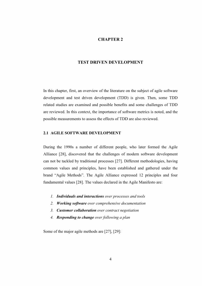
brand “Agile Methods”. The Agile Alliance expressed 12 principles and four

fundamental values [28]. The values declared in the Agile Manifesto are:

1. Individuals and interactions over processes and tools

2. Working software over comprehensive documentation

3. Customer collaboration over contract negotiation

4. Responding to change over following a plan

Some of the major agile methods are [27], [29]:

5

1. Extreme Programming: Extreme Programming (XP), the most popular

agile software development methodology, was developed by Kent Beck.

The five values of XP are: Communication, Simplicity, Feedback,

Courage and Respect. These values denotes communicating with customer

and within the team, keeping the design simple and clean, getting instant

feedback by starting testing on day one, courageously responding to

changing requirements and technology and responding fellow

programmers and their work [35].

2. Scrum: Scrum is a lightweight methodology initially created by Ken

Schwaber and Jeff Sutherland. Scrum method provides a project

management framework including daily meetings for coordination and

integration that do not last for more than 15 minutes and iterative

development in 30 day periods (called a sprint cycle).

3. Crystal Methods: The crystal family of methodologies was developed by

Alistair Cockburn who is a methodology archeologist. This is called

crystal family because methodology differs according to the size of the

team and the criticality of the project. The method focuses on people,

interaction, collaboration, cooperation, skills, talents and communication

as first order effects.

4. Feature Driven Development (FDD): FDD, developed by Jeff De Luca

and Peter Coad, is composed of five sub-processes each defined with entry

and exit criteria. These steps focuses on developing object models and

sequence diagrams, building a feature list, planning by feature, iteratively

designing by feature and building by feature respectively.

Besides the above methods, there are other agile methods such as Dynamic

Systems Development Method (DSDM), Lean Development, Adaptive Software

Development (ASD), Agile Modeling, Agile Unified Process (AUP).

6

2.2 INTRODUCTION TO TDD

Test Driven Development [2] is an approach, adopted in many agile software

development techniques that involves writing automated tests before the

implementation of the code and then coding in the guidance of the written tests.

The developer executes these automated tests repeatedly so that he gets

immediate feedback from failed or successful tests to judge progress.

TDD can be described mainly in five steps [2], [3]:

1. Quickly add a test: When a new functionality is to be implemented, the

code that will test that the functionality works is written before

implementing the functionality itself.

2. Run all tests and see the new one fail: Since the implementation of the

new feature hasn’t been done yet, the new test has to fail. This shows that

the new test does not mistakenly pass without requiring any new code.

3. Write some code: In this step, the developer writes the simplest code that

is only enough to pass the test. No more functionality should be

implemented. The perfection of the code is not much important in this

step.

4. Run all tests and see the new one pass: This validates that the newly

added code satisfies the requirements of the new feature.

5. Refactor: Now, the perfection of the code can be considered. Refactoring

means improving the quality of the working code without changing its

external behavior. It can be done whenever we think that the code is poor

but it must be done in case of duplications and ambiguity in code.

7

This cycle is repeated until the last feature is added to the software; that is, until

the last requirement is satisfied. The step sizes can be smaller or larger. The

developer can add a large feature in one cycle or split it into smaller testable

steps. Running all tests in every cycle may be time consuming in some cases so

instead of this, only newly added tests may be run in each cycle. The overall test

execution can be done periodically throughout the day, as shown in Figure 2.1

[4].

Figure 2.1 – TDD Cycle [4]

8

2.3 BENEFITS OF TDD

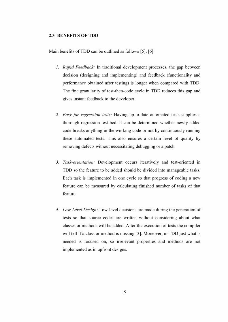
Main benefits of TDD can be outlined as follows [5], [6]:

1. Rapid Feedback: In traditional development processes, the gap between

decision (designing and implementing) and feedback (functionality and

performance obtained after testing) is longer when compared with TDD.

The fine granularity of test-then-code cycle in TDD reduces this gap and

gives instant feedback to the developer.

2. Easy for regression tests: Having up-to-date automated tests supplies a

thorough regression test bed. It can be determined whether newly added

code breaks anything in the working code or not by continuously running

these automated tests. This also ensures a certain level of quality by

removing defects without necessitating debugging or a patch.

3. Task-orientation: Development occurs iteratively and test-oriented in

TDD so the feature to be added should be divided into manageable tasks.

Each task is implemented in one cycle so that progress of coding a new

feature can be measured by calculating finished number of tasks of that

feature.

4. Low-Level Design: Low-level decisions are made during the generation of

tests so that source codes are written without considering about what

classes or methods will be added. After the execution of tests the compiler

will tell if a class or method is missing [3]. Moreover, in TDD just what is

needed is focused on, so irrelevant properties and methods are not

implemented as in upfront designs.

9

2.4 CHALLENGES OF TDD

Some important challenges of TDD have been categorized as follows:

1. Database Projects: Applying Test Driven Development (TDD) to a

project including network environment or database [7] is very difficult

because the database and network environment may have not been

developed before the beginning of the project. Thus, automated tests can

not be processed till these environments are implemented. Preparation of

mock objects for this purpose can also take too much time and effort.

2. Developer’s familiarity: Since the developers are accustomed to use

traditional Test-Last development techniques, getting familiar with writing

tests first can be difficult for them.

3. Overall Test Duration: In main TDD cycle, all tests are repeatedly

executed in case of a new test addition. If the overall test execution takes,

for example an hour, the overall duration of the project significantly

increases, proportionally the cost of the project increases and also the

motivation of the developers decreases.

4. Insufficient Tool Support: As mentioned above overall test duration is a

critical aspect for TDD. Hence, tool support for the automation of the unit

tests becomes very important because utilization of a software tool to

write automated unit tests significantly reduces the overall duration.

5. Embedded Systems: In the lowest level embedded systems [8], the

resources for running test frameworks are limited such that these systems

have no operating system and also there is no use of object oriented

languages (C#, C++ or Java) in them. Moreover, direct interaction of

software and hardware makes practicing TDD in embedded systems much

10

more difficult. Hardware functions must also be automated to be able to

run unit tests in an automated fashion.

6. GUI Applications: Automating the tests for the Graphical User Interface

(GUI) aspects of the system is very hard [9]. For example, writing

automated unit tests for the code that implements a mouse action or gives

a visual output is useless. Manual testing of complex GUI applications in

TDD fashion (periodically run manual GUI tests with other automated

unit tests) is also possible but time consuming; that is, expensive.

2.5 SOFTWARE METRICS

Recent development of software in organizations brings the necessity of

improvement in the management of software development projects. To be able to

improve something, first you have to know what the current situation is and to

know that, you have to measure. As Lord Kelvin mentioned

(http://www.qualitydigest.com/sept97/html/qmanage.html): “When you can

measure what you are speaking about, and express it in numbers, you know

something about it; but when you cannot measure it, when you cannot express it

in numbers, your knowledge is of a meager and unsatisfactory kind; it may be the

beginning of knowledge, but you have scarcely in your thoughts advanced to the

state of Science”. In literature, measurements of the properties such as,

productivity, quality and reliability, of a software system are called software

metrics. These metrics allow the organizations to quantify their schedule, work

effort, product size, project status and quality performance [13]. Utilization of the

recorded metrics in past projects also improves the future work estimates.

One set of software metrics are objectively measurable, code or any other kind of

product metrics. These metrics are obtained by measuring any means of product

at a particular point in time [23]. A second set of metrics, called process metrics,

11

are related to concepts such as maintainability, comprehensibility and reliability

and also involve people and the environment. Different from product metrics,

process metrics measure the change during the whole process.

Product metrics are calculated by measuring the product at a specific time during

the whole development cycle. This product can be the whole code, functions in

the code, interactions between functions, classes or methods in classes. Many

product metrics have been proposed in the literature (a comprehensive list of

product metrics can be found in Appendix A). These metrics mainly measure the

size of the project, functions and how functions interact, classes and how classes

interact, methods and how methods interact and inheritance. Some of the product

metrics used for measuring productivity and quality are examined in the

following sub-sections in a more detailed way.

According to the Merriam-Webster online dictionary, a process is a series of

actions or operations conducting to an end. Thus, the meaning of the process in

business can be stated as “a structured set of activities that leads to the production

of a product or a service for a particular customer or customers”. The act of

defining, planning, visualizing, measuring, controlling, reporting and improving

these business processes called process management. Process management has

become the main part of software quality management since 1970’s [26].

Product metrics are measured at specific points of time and do not give

information about the movement between these points. The whole process can not

be understood from instantaneous calculations. The process has a time rate of

change and the evaluation of this change can be made by using software process

metrics [23].

Many process metrics have been defined and discussed in the literature. Some

CMMI-based metrics are given in Table A.2 in Appendix A.

12

Besides product and process metrics classification, software metrics can also be

classified according to what property they measure. In this study, two

development projects are compared in terms of productivity and quality. Hence,

in the next sub-section, software productivity and quality metrics will be

discussed.

2.5.1 SOFTWARE PRODUCTIVITY METRICS

Productivity is measured as the ratio of units of output produced divided by units

of input to the production process. Here, units of output denote the work done;

units of input denote the effort spent to do that work. For software, work done can

be expressed in terms of the source code produced (Lines of Code), function

points and documentation pages. Effort spent is measured as the overall time

spent on that project by the project team and it is calculated in staff-hours [14].

2.5.1.1 LINES OF CODE (LOC)

LOC is the metric used to measure the size of the source code and is measured by

counting the code lines. The source code lines can be calculated in two ways [20]:

1. Physical LOC: Physical LOC is measured by counting all lines in the code

regardless of that the line consists of an instruction or not. The physical

LOC metric can be automatically counted by the compilers or code

generator tools and this metric can be used in a large number of software

estimating tools. On the other hand, physical LOC metric does not exclude

comments, blank lines and dead code which may be misleading for effort

calculation. Also, there is no direct mathematical conversion of this metric

to logical LOC or function points metric.

2. Logical LOC: Logical LOC is measured by counting the number of

software instructions in each line. Explicitly, if a line includes two

13

instructions, that line is counted as two; if there is one instruction in two

lines, that lines are counted as one. Logical LOC is also used in a number

of software estimating tools, but calculation of it is not as easy as physical

LOC. Since it is the count of instructions, it is not extensively automated

for counting. Different from physical LOC, logical LOC does not include

comments, blanks or dead code. Moreover, it can be converted into

function point metrics.

In general, LOC metric is easy to calculate; more widely used in effort calculation

and has tool support. Nevertheless, since it is measurement of size by only

measuring the code lines, LOC metric is not appropriate for some visual

languages and poor choice for full life-cycle studies. Furthermore, LOC metric is

a programming language dependent metric [14], so can not be used in the

comparison of software systems using different languages. Thus, if a software

program is implemented using two languages such as C# and Java, LOC of each

language shall be counted separately.

2.5.1.2 FUNCTION POINTS (FP)

As an alternative to measuring simply the lines of code, Allan J. Albrecht

originally suggested measuring the “function” that the software is performing

[15]. The amount of the performed function is evaluated in terms of absorbed and

produced data and it is quantified as function points.

In recent studies performed in METU on functional software measurement and

effort estimation [30, 31], Gencel states that, after the development of Albrecht’s

original method, various new functional size measurement methods have been

suggested and widely used. The methods found in the literature are given in

Appendix B.

14

A need for the standardization of these methods was evolved to prevent the

inconsistencies between them [30]. Thus, the common principles of these

methods are established and published by the International Standards

Organization (ISO). Four of the methods given in Appendix B; namely COSMIC

Full Function Points, IFPUG Function Point Analysis, Mark II Function Point

Analysis and NESMA Function Point Analysis, have been approved by this

organization till now.

IFPUG Function Point Analysis is a relatively simple model of Function Point

Analysis method based on weighting four types of functions, Input, Output,

Inquiry and File, with an adjustment factor [15]. With the improvements in years

[45], the “File” attribute has been divided into two as “the internal logical file”

and “the external interface file”. These five function types are named as External

Input, External Output, External Inquiry, Internal Logical File and External

Interface File and they are classified into two; data function and transactional

function types [44].

Data function types are:

1. Internal Logical File (ILF): ILF is the data or control information

internally stored and used in the boundary of the software application.

2. External Interface File (EIF): EIF is the data or control information stored

in another application but used by the application through an interface.

EIF must be an ILF of another application.

Transactional function types are:

1. External Input (EI): EI is the data or control information that comes from

outside the software system.

15

2. External Output (EO): EO is the data or control information that is sent

outside the software system.

3. External Inquiry (EQ): EQ is an input-output combination that results in

data retrieval. Input data is formatted and sent outside the application

without added value. No ILF is maintained during EQ processing.

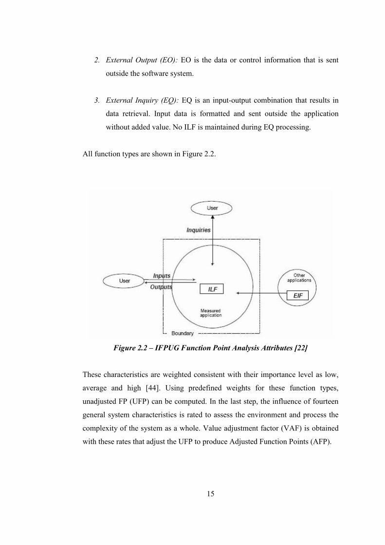
All function types are shown in Figure 2.2.

Figure 2.2 – IFPUG Function Point Analysis Attributes [22]

These characteristics are weighted consistent with their importance level as low,

average and high [44]. Using predefined weights for these function types,

unadjusted FP (UFP) can be computed. In the last step, the influence of fourteen

general system characteristics is rated to assess the environment and process the

complexity of the system as a whole. Value adjustment factor (VAF) is obtained

with these rates that adjust the UFP to produce Adjusted Function Points (AFP).

16

Mark II Function Point Analysis (Mk II FPA) was proposed in 1988 by Charles

Symons [40]. It is based on the assumption that the system size is determined by

three components: Information processing size, technical complexity factor and

environmental factors. Allan Albrecht’s “Function Point Analysis” method is

based on the first two of these components and the purpose of the proposed new

approach is to overcome the weakness of regular FPA. The system is divided into

logical transactions in Mark II FPA method [41]. Each logical transaction is

composed of Input Data Element Types, Data Entity Types Referenced and

Output Data Element Types and FP is calculated by counting these types. This

method can be used mainly to improve estimation of development of

computerized business information systems [40].

Nesma Function Point Analysis method is based on the principles of the IFPUG

FPA [46]. The types of user functions used in NESMA FPA are same as the types

in IFPUG: External Input, External Output, External Inquiry, Internal Logical File

and External Interface File as in the IFPUG FPA. Different from the detailed

function point count (FPC) in IFPUG, NESMA FPA additionally provides

estimated function point count and the indicative function point count. The only

difference in estimated FPC from the detailed FPC, is that the function

complexities are evaluated by default. In the indicative FPC, function point is

evaluated by using only ILFs and EIFs.

COSMIC Full Function Points (FFP) method presented by Alain Abran[41] was

designed to measure functional size of real-time software in addition to the

business application software. It provides higher level model of abstraction, richer

functional size model and simpler measurement function than the previous

methods. This measurement is based on the Functional User Requirements (FUR)

of the system, which is a sub-set of user requirements including data transfer and

data transformation; excluding quality and technical requirements [42]. COSMIC

FFP is calculated by counting data movements; Entry, Exit, Read, and Write.

17

Besides the approved methods mentioned above, Ç. Gencel, in her PhD study in

METU Informatics Institute [30], has proposed a new functional size

measurement (FSM) method based on the findings of the literature reviews and

the results of the case studies, called architectural dimensions based FSM

(ARCHI-DIM) [30]. Development projects, enhancement projects and also

applications can be measured by this method. The purpose and the boundaries of

measurement are identified and so the FURs are chosen according to the

measurement type, purpose and the boundaries of the measurement. After

identifying these elementary processes, base functional components (BFCs)

within the FURs, data groups, data element types, constituent parts of BFCs and

BFC types of the Constituent Parts of BFCs are identified and measured to

construct the Archi-Dim model and calculate Archi-Dim functional size of the

project.

Archi-Dim uses vectors of measures instead of counting data elements and

combining these counts. Functionality is evaluated by considering four types;

Interface, Control Process, Algorithmic Process and Permanent Data

Access/Storage. This functionality types provides measuring components of

different application domains. One of the main contribution of Archi-Dim is that

the effort for each functionality specified above can be measured independently.

Measuring functionality separately allows user to represent the application

domain of the software as data strong, control strong, etc. [30].

In general, FP is a language independent metric; that is, FP value of a software

system is computed regardless of the programming language used in that system

[20]. Moreover, besides coding, FP measures documentation activities, defects

found in requirements, design or analysis stages. Thus, FP is a better choice than

LOC for full life-cycle analysis. As LOC metric, FP has also tool support for

software cost estimating. Since FP includes measurement of interactions of the

system and files, it can be considered as a good choice for software reuse

analysis.

18

It has also been argued in the literature that, in contrast to its advantages, FP has

some weaknesses as well [20]: Function point calculation is a subjective

calculation method and to be precise enough, counting requires function point

specialists. It is not as easy as LOC calculation and automation is not possible in

most of the cases, so FP can be time-consuming and expensive. Lastly, it has been

claimed [20] that FP calculation is not suitable for small projects; projects below

15 function points in size.

2.5.1.3 DOCUMENTATION PAGES

Document pages metric is the measurement of all documents that actively support

the development or the usage of the product. Documents may be composed of

hard copies, screen shots, texts and graphics used to carry information to people.

In a software development project, typically measured documents are

requirements specifications, architectural and design documents, test description

and test plan documents, data definitions, user manuals, reference manuals,

tutorials, training guides and installation and maintenance manuals. The

documents that are not preserved but require a significant amount of effort to

produce should also be evaluated. Proposals, schedules, budgets, project plans

and reports are the examples of this kind of documents. There are three main

aspects while counting documentation [14]:

1. Document Page Count: Total number of nonblank pages contained in a

hard copy documentation or document screens in computer file

documentation can be considered as document page count. It is an integer

value and partially filled pages are counted as full pages.

2. Document Page Size: Edge-to-edge dimensions of hard copy documents

shall be measured and specified in some units. Similarly, for electronically

19

displayed documents, screen width and screen height shall be measured.

Average number of characters per line is measured as screen width; the

number of lines per screen is measured as screen height.

3. Document Token Count: Three kinds of token shall be counted: words,

ideograms, and graphics. Contractions, such as “can’t”, “won’t”,

numerical values, such as 35, 32.45, acronyms, roman numerals and

abbreviations are counted as a single word. Punctuation marks are

ignored. Ideograms are the symbols representing ideas such as equations.

Graphs, tables, figures, charts and pictures are considered as all graphics

and counted in the graphic token count.

Documentation pages metric clearly measures and illustrates the documentation

effort of the software development project and also can be used to estimate the

functionality size of the project by looking at requirement specifications and

design specifications documents. However, this metric is still very weak in the

implementation effort calculation. Values for the coding part obtained using this

metric are only the estimations from documentation. Thus, documentation pages

metric is generally used as an associative metric to LOC metric or FP metric.

Furthermore, as agile methods, in general, emphasize “people over

documentation”, TDD does not generally aim to increase the amount of

documentation produced in a software project.

2.5.2 SOFTWARE QUALITY METRICS

Software quality is the evaluation of a software system in accordance with a

desired and clearly defined set of attributes. Software quality metrics are the

numerical interpretation of these quality attributes. The judgment of whether the

quality requirements of a project are being met can be made by the use of

software quality metrics. Furthermore, utilization of numerical values in the

20

assessment and control of software quality reduces subjectivity by making the

software quality attributes more noticeable [16].

In this section, seven most commonly used quality metrics will be described.

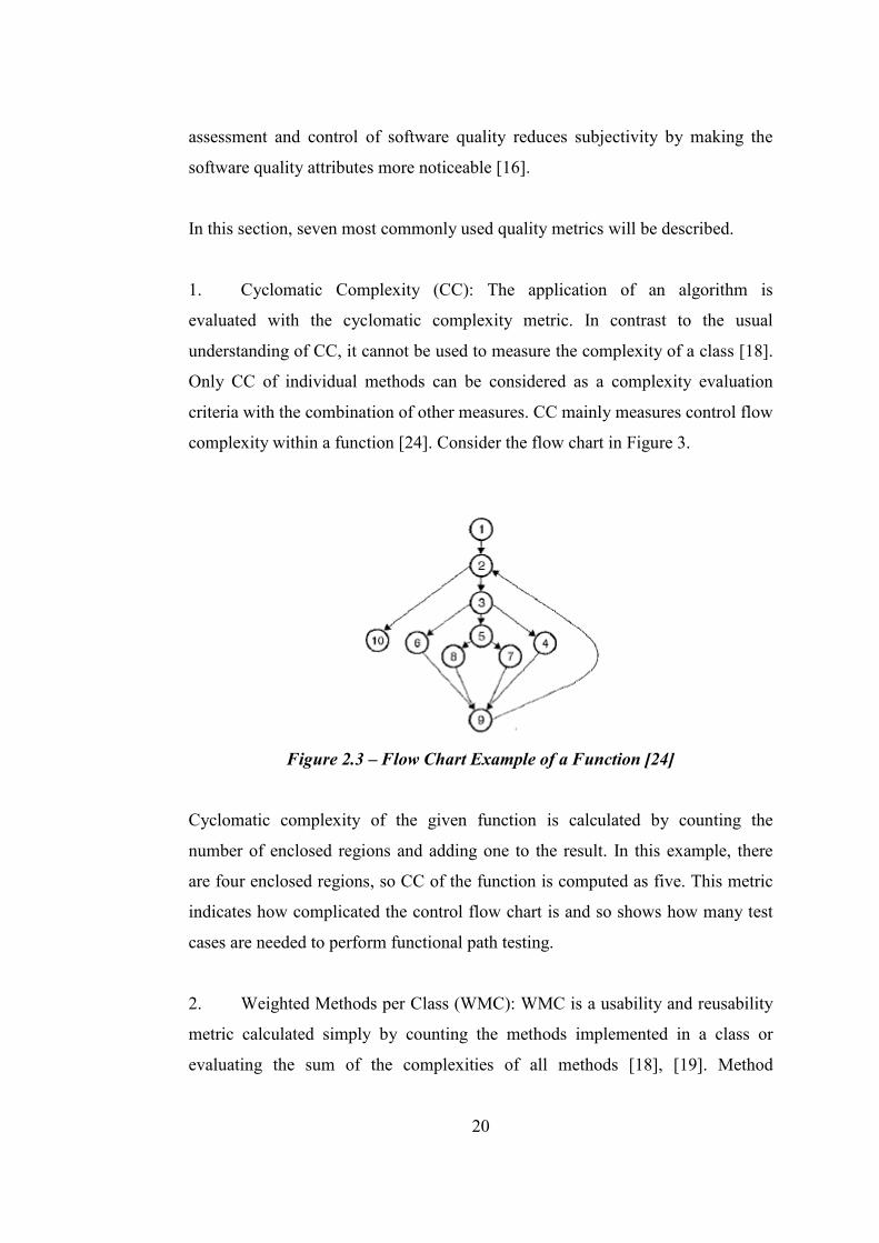
1. Cyclomatic Complexity (CC): The application of an algorithm is

evaluated with the cyclomatic complexity metric. In contrast to the usual

understanding of CC, it cannot be used to measure the complexity of a class [18].

Only CC of individual methods can be considered as a complexity evaluation

criteria with the combination of other measures. CC mainly measures control flow

complexity within a function [24]. Consider the flow chart in Figure 3.

Figure 2.3 – Flow Chart Example of a Function [24]

Cyclomatic complexity of the given function is calculated by counting the

number of enclosed regions and adding one to the result. In this example, there

are four enclosed regions, so CC of the function is computed as five. This metric

indicates how complicated the control flow chart is and so shows how many test

cases are needed to perform functional path testing.

2. Weighted Methods per Class (WMC): WMC is a usability and reusability

metric calculated simply by counting the methods implemented in a class or

evaluating the sum of the complexities of all methods [18], [19]. Method

21

complexity can be measured by CC, as mentioned in the Cyclomatic Complexity

sub-section. Both number of methods and sum of complexities are used for

estimating how much time and effort is required to develop and maintain the

class. Increasing WMC value of a class has a negative effect on inheriting classes

and also increases the effort and time needed for testing and maintenance.

Moreover, classes with high number of methods have low cohesion which limits

the possibility of reuse.

3. Response for a Class (RFC): Response for a class is used for measuring

complexity in terms of the amount of communication between the methods of the

class with methods in the same class or other classes [19]. If the RFC value is

high; that is, if the number of methods that can be invoked from a class through

messages is high, debugging becomes much harder and the class turns into a less

understandable one. Hence, usability and the testability of the class become more

complicated.

4. Lack of Cohesion of Methods (LCOM): LCOM measures the cohesion of

a class by evaluating inter-relatedness of the methods [18], [19]. There are two

different ways of measuring cohesion.

� For each data field, calculate the percentage of the methods use that data

field to all methods in a class. Greater percentages mean greater cohesion

of data and methods in the class.

� Subtract the number of non-similar method pairs from the number of

similar method pairs. The larger number of similar methods shows the

more cohesiveness of the class.

Lack of cohesion increases complexity and is evidence for the necessity of

dividing that class into two or more subclasses with increased cohesion.

5. Coupling between Objects (CBO): CBO is the count of the number of

coupled classes to a class [19]. Smaller CBO values indicate that the class is more

independent and it is easier to reuse the class in another application. Thus, CBO

22

values should be kept at minimum to improve modularity and provide

encapsulation. Increase in the number of couples, increases the understandability

of the class and also sensitivity of the class to changes. Therefore, debugging and

maintenance become more difficult.

6. Depth of Inheritance Tree (DIT): The maximum length from the class

node to the root of the tree is calculated as the depth of a class within the

inheritance hierarchy [18]. With increasing DIT value, understandability of a

class decreases and also tests become more complex because deeper trees have

greater design complexity and they are composed of more methods and classes.

Contrarily, the potential for reuse of inherited methods increases. In general, this

metric relates to reusability, understandability and testability.

7. Number of Children (NOC): The number of children is the number of

immediate subclasses inferior to another class in the hierarchy [18]. NOC metric

primarily measures usability. The Greater the NOC value, the greater the reuse.

On the contrary, increasing number of children, makes testing of that class more

complex, thus testing time of the class increases. Hence, NOC can also be

considered as an evaluation criteria for the design of the class.

In a recent study performed in METU, the effect of design patterns on object-

oriented metrics and software error-pronenses was investigated [32]. Here, B.

Aydınoz stated that the WMC, DIT, NOC, RFC and CBO indicates the

complexities of the software classes and are important for software fault

tolerance, whereas LCOM is a class cohesion metric which has a weak relation

with fault-pronenses. In an empirical experiment conducted on eight medium

sized school projects, the results show that these five metrics (WMC, DIT, NOC,

RFC and CBO) are useful quality indicators for predicting error prone classes

[34].

23

Since WMC shows the number of methods and the complexity of methods,

increase in the WMC value makes the class hard to maintain and also hard to

repair [32]. This shows that the class should be divided into two or more classes.

It is also mentioned that the RFC is a good indicator for OO faults because it

additionally counts the associations between objects and methods. While the

higher DIT value makes the classes more error prone, the higher NOC value

makes the classes less error prone [11]. This is explained by the greater attention

given to the classes with high NOC during implementation [32]. Moreover,

classes with high export coupling values are not more likely to be error prone [11,

32]. On the other hand high import coupling values are directly related with error

proneness, so CBO metric should be considered while measuring quality in terms

of error-proneness.

2.6 THE EFFECTS OF TDD ON SOFTWARE METRICS

The general belief about TDD is that TDD leads to an increase in developer’s

productivity and improves the internal quality of the software; but there are also

counter ideas and studies.

Developer productivity in a software project is defined as code developed per unit

time. There are a few comparison studies looking at whether TDD increases

productivity or not. Two of them that have come from academia stated that Test-

First development significantly increased the productivity of the developers. In

one of them [10], it was observed that the Test-First team (the team using TDD)

spent 57% less effort per feature than the Test-Last team. In another study [5], the

conclusion was that TDD led to 21% - 28% increase in productivity.

On the contrary, the results coming from industry do not, in general, support the

results from academia. In the research conducted by a group of experienced

programmers [1], developer productivity was evaluated by comparing the efforts

24

of the groups with the estimated effort provided by a group of industry experts.

As compared to the estimated time, both projects took longer time, but when

compared to each other there was no significant difference between them. The

other study compared two case studies performed at Microsoft using TDD with

the early comparable works at Microsoft using non-TDD [4]. In project A, which

was carried out in Windows division, it was seen that TDD led to an increase in

the order of 25-35% in development time. The development time increase in

Project B, performed in MSN division, was 15%.

There are also contradicting results for internal quality measurements coming

from both academia and industry.

In the industrial experiment [1], software quality was investigated by calculating

the frequency of unplanned test failures. The frequency of unplanned test failures

was evaluated both in developer/unit test level and customer/acceptance test level.

As in developer productivity comparison mentioned above, there was no

significant difference between test-first and test-last groups.

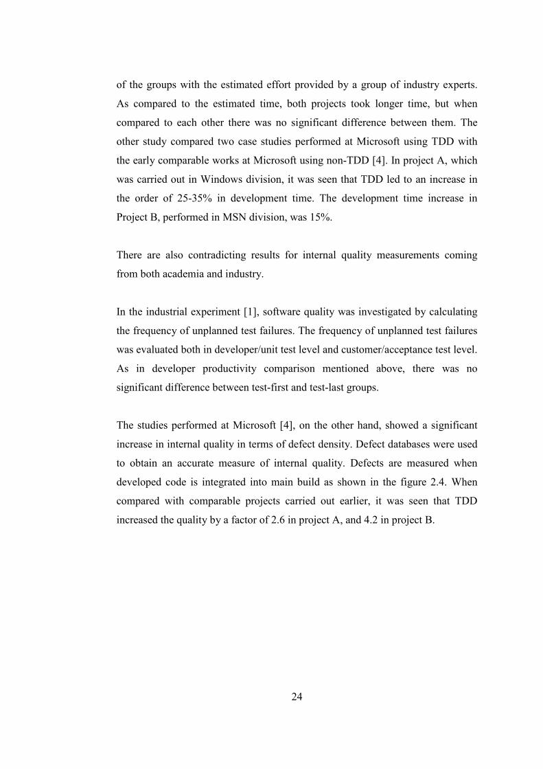
The studies performed at Microsoft [4], on the other hand, showed a significant

increase in internal quality in terms of defect density. Defect databases were used

to obtain an accurate measure of internal quality. Defects are measured when

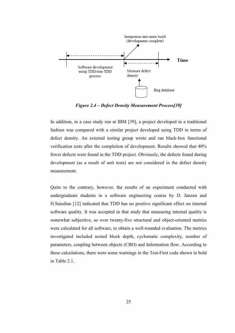
developed code is integrated into main build as shown in the figure 2.4. When

compared with comparable projects carried out earlier, it was seen that TDD

increased the quality by a factor of 2.6 in project A, and 4.2 in project B.

25

Figure 2.4 – Defect Density Measurement Process[39]

In addition, in a case study run at IBM [39], a project developed in a traditional

fashion was compared with a similar project developed using TDD in terms of

defect density. An external testing group wrote and ran black-box functional

verification tests after the completion of development. Results showed that 40%

fewer defects were found in the TDD project. Obviously, the defects found during

development (as a result of unit tests) are not considered in the defect density

measurement.

Quite to the contrary, however, the results of an experiment conducted with

undergraduate students in a software engineering course by D. Janzen and

H.Saiedian [12] indicated that TDD has no positive significant effect on internal

software quality. It was accepted in that study that measuring internal quality is

somewhat subjective, so over twenty-five structural and object-oriented metrics

were calculated for all software, to obtain a well-rounded evaluation. The metrics

investigated included nested block depth, cyclomatic complexity, number of

parameters, coupling between objects (CBO) and Information flow. According to

these calculations, there were some warnings in the Test-First code shown in bold

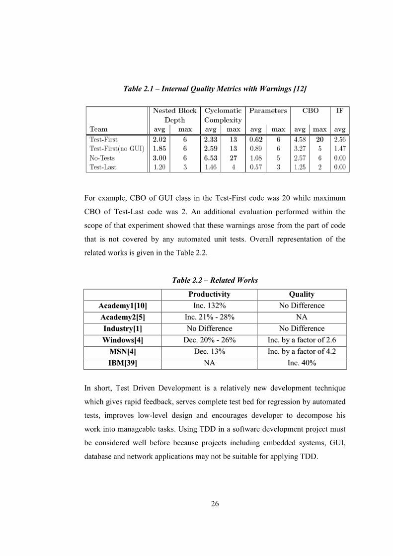
in Table 2.1.

26

Table 2.1 – Internal Quality Metrics with Warnings [12]

For example, CBO of GUI class in the Test-First code was 20 while maximum

CBO of Test-Last code was 2. An additional evaluation performed within the

scope of that experiment showed that these warnings arose from the part of code

that is not covered by any automated unit tests. Overall representation of the

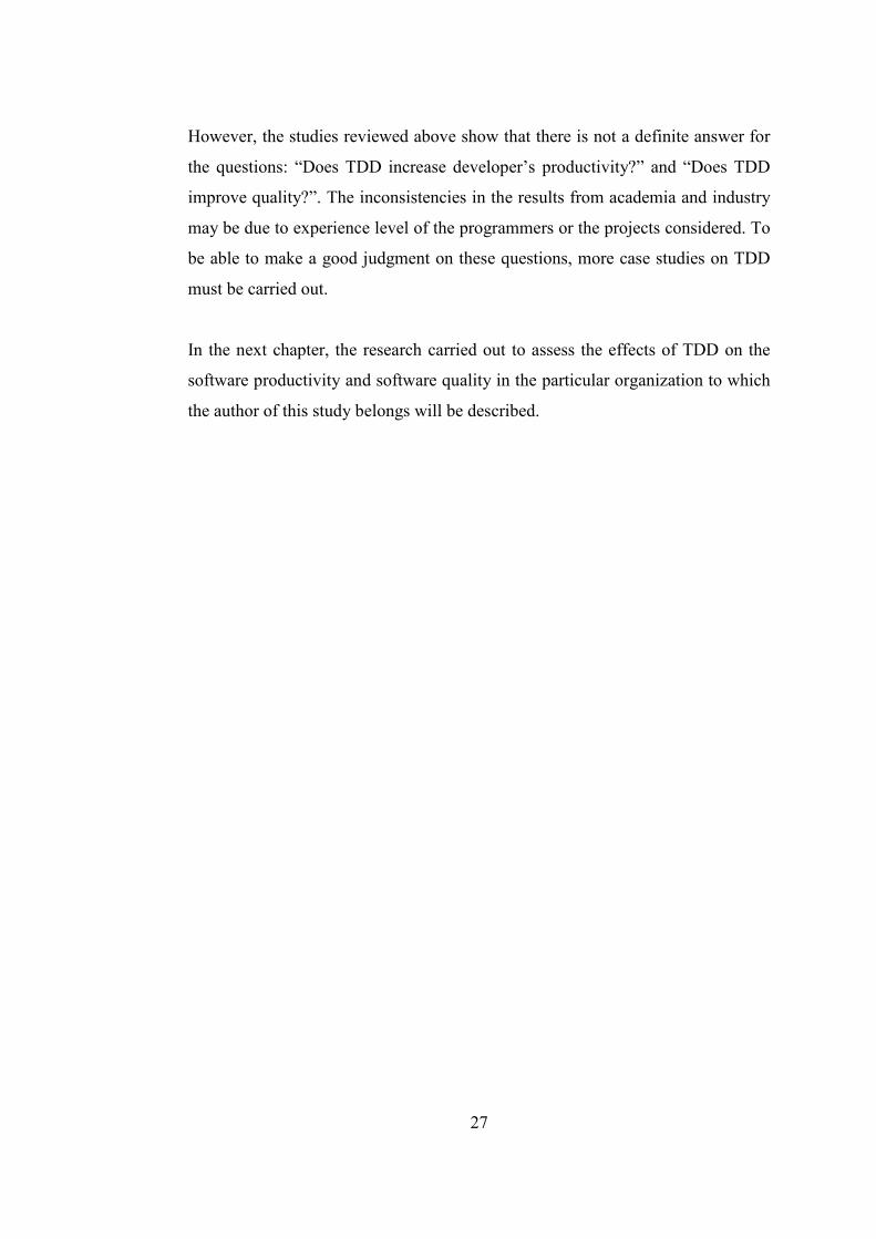
related works is given in the Table 2.2.

Table 2.2 – Related Works

Productivity Quality

AAccaaddeemmyy11[[1100]] IInncc.. 113322%% NNoo DDiiffffeerreennccee

AAccaaddeemmyy22[[55]] IInncc.. 2211%% -- 2288%% NNAA

IInndduussttrryy[[11]] NNoo DDiiffffeerreennccee NNoo DDiiffffeerreennccee

WWiinnddoowwss[[44]] DDeecc.. 2200%% -- 2266%% IInncc.. bbyy aa ffaaccttoorr ooff 22..66

MMSSNN[[44]] DDeecc.. 1133%% IInncc.. bbyy aa ffaaccttoorr ooff 44..22

IIBBMM[[3399]] NNAA IInncc.. 4400%%

In short, Test Driven Development is a relatively new development technique

which gives rapid feedback, serves complete test bed for regression by automated

tests, improves low-level design and encourages developer to decompose his

work into manageable tasks. Using TDD in a software development project must

be considered well before because projects including embedded systems, GUI,

database and network applications may not be suitable for applying TDD.

27

However, the studies reviewed above show that there is not a definite answer for

the questions: “Does TDD increase developer’s productivity?” and “Does TDD

improve quality?”. The inconsistencies in the results from academia and industry

may be due to experience level of the programmers or the projects considered. To

be able to make a good judgment on these questions, more case studies on TDD

must be carried out.

In the next chapter, the research carried out to assess the effects of TDD on the

software productivity and software quality in the particular organization to which

the author of this study belongs will be described.

28

CHAPTER 3

ASSESSMENT OF THE EFFECTS OF TDD

3.1 EXPERIMENTAL DESIGN

For the assessment of the effects of TDD on software development productivity

and software quality, two similar software development projects were

implemented in object-oriented manner by using two different development

techniques; project A with Test Driven Development, project B with Test-Last

development technique.

Project A is the development of a simulator program that will behave as the

STRELETS unit and simulate all communication with the interfaces of this unit.

STRELETS unit communicate with its interfaces using Serial Input/Output (SIO)

and TCP/IP protocols. This simulator program was developed by using C# in the

.NET 2003 platform.

Project B is also a simulator program that will behave as the LRF unit and

simulate all communication with the interfaces of this unit. Moreover, this

program was developed by using C# in the .NET 2003 platform to be able to

make comparison between TDD and Test-Last development independent of the

programming language and the development platform. As in STRELETS

simulator in project A, LRF simulator communicate using Serial Input/Output

(SIO) and TCP/IP protocols.

29

LOC produced per staff-hours is measured during the development processes in

both projects and used for the evaluation of productivity. LOC metric is used for

size measurement together with FP calculation because our aim is evaluating not

only the size of code but also the interactions in the code.

Since TDD emphasizes working code over comprehensive documentation,

documentation pages metric is not measured in this research. Instead of this

metric, effort distribution percentage metrics for both processes are measured.

These metrics show the proportion of the effort spent (in staff-hours) for

documentation, testing and coding.

Defects found during implementation are also measured to assess the effects of

TDD to the internal quality by means of defect density. Both defects found per

unit time and defects found per KLOC are evaluated to be able to assess the rate

change of defects with time and size. Moreover, some quality product metrics

such as cyclomatic complexity, weighted methods per class, response for a class,

lack of cohesion of methods, coupling between objects, depth of inheritance tree

and number of children, are measured at the end of both projects for assessment

of overall software quality. It is mentioned that the non-Object-Oriented metrics

are ineffective for the assessment of OO software design because they have

mathematical properties for the traditional function based software design and fail

to display predictable behaviour of OO software [33]. Thus, WMC, DIT, NOC,

RFC, CBO and LCOM metrics are chosen in this study because they are

specifically for object-oriented systems [33] and also they are suitable and enough

for the evaluation of coupling, cohesion and inheritance [18]. CC metric is used

to measure the control flow complexity [24].

Besides the comparison of project A and project B, the TDD project is also

compared with an early work, project C, performed at ASELSAN A.Ş. Project C

is developed by using Test-Last development technique. Since project A and the

early work are not similar in size, a productivity comparison would not be

30

meaningful. Furthermore, defect density measurement for the project C is not

available so these projects are compared only in terms of product quality by using

the above mentioned software product quality metrics.

In short, the product metrics, Cyclomatic Complexity, Weighted Methods per

Class, Response For a Class, Lack of Cohesion Of Methods, Coupling Between

Objects, Depth of Inheritance and Number Of Children have been evaluated for

projects A, B and C, and the process metrics, LOCs / Staff-Hours, FP / Staff-

Hours, Defects Found / Staff-Hours, Defects Found / LOCs and Effort Percentage

have been evaluated for projects A and B.

3.2 EXPERIMENT RESULTS

3.2.1 PROJECT A – RESULTS OF THE TDD PROJECT

STRELETS simulator program was developed by using TDD at ASELSAN A.Ş.

Within the scope of this thesis, it is used for assessing the effects of TDD on

software metrics. Further information about the STRELETS simulator program

can be found in the Appendix G.

Automated unit tests are done with the NUnit 2.4.8 [36] program in the project.

The increments in the project are planned and the workload is equally distributed

between these iterations. In an iteration, first, new tests are added to the project by

using NUnit framework. These tests are run and they are all failed. The necessary

code is implemented till all the newly added tests are passed. After all code is

implemented for that iteration, automated functional tests are added and also

previously added functional tests are updated. Then all tests in the code base are

run to see whether the previously implemented code is affected from the newly

added code. This part is the integration of the new increment to the main build.

The project was completed in eight iterations and the products obtained each

31

iteration were given a new version number. Process metrics graphs were prepared

by using these versions. Overall representation of the evaluated process metrics

for each version can be found in the Appendix F.

As mentioned in the “Challenges of TDD” section automated GUI testing is a

very hard process. In this project, user interface testing is done by checking GUI

parameters whereas possible. When it is not possible, half-automated tests

(requiring tester to declare pass/fail) are added to the GUI test steps which extend

the overall test duration.

The LOCs versus staff hours graph is shown in Figure 3.1. In the second

increment, the serial communication class is implemented. The methods

necessary to open a serial communication make the sharp increase in this

iteration. Besides second iteration, the LOC changes are very close to each other.

LOCs vs. Staff Hours

0; 017; 422

37; 1720

98; 3686127; 4485114; 4214

78; 3015

64; 257251; 2212

0500

100015002000250030003500400045005000

0 20 40 60 80 100 120 140

Staff-Hours

LOCs

Figure 3.1 – LOCs versus Staff-Hours for Project A

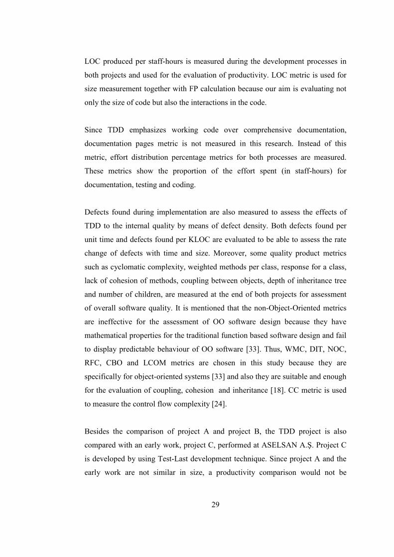
Second process metric evaluated is the function points per staff hours. The equal

distribution of workload between iterations can easily be seen in Figure 3.2. Here

function points are calculated according to the IFPUG FPA and the calculation

details are given in the Appendix H.

32

Function Points vs. Staff Hours

0; 017; 8

37; 1651; 24

64; 3478; 42

98; 53114; 59

127; 70

0

10

20

30

40

50

60

70

80

0 20 40 60 80 100 120 140

Staff-Hours

FPs

Figure 3.2 – Function Points versus Staff-Hours for Project A

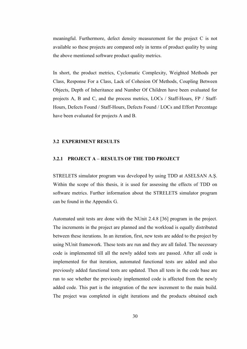
In the project, the process quality is measured by means of defects density. As

seen, defects are equally distributed all over the project.

Defects Found vs. Staff Hours

0; 0

114; 26127; 29

98; 24

78; 1864; 15

51; 12

37; 9

17; 50

5

10

15

20

25

30

35

0 20 40 60 80 100 120 140

Staff-Hours

# of Defects

Figure 3.3 –Defects Found versus Staff-Hours for Project A

The slope of the defects density versus LOCs graph is higher in the first and sixth

iterations. The defects in the first increment are originated from the disconnect

33

method in the Ethernet client class. The complex algorithms in the Combat Mode

class cause the increase in the sixth iteration.

Defects Found vs. LOCs

0; 0

4485; 294214; 26

3686; 24

3015; 182572; 15

2212; 12

422; 5

1720; 9

0

5

10

15

20

25

30

35

0 1000 2000 3000 4000 5000

LOCs

# of Defects

Figure 3.4 –Defects Found versus Line of Codes for Project A

29 total defects were found in the project A. These errors are including both

defects found in automated unit tests and in automated functional tests.

Separately, 12 defects were found by functional tests, where 17 defects were

found by unit tests.

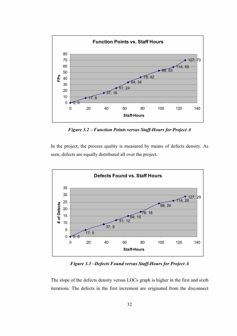
The effort percentage metric was measured to be able to see whether TDD

decreases the time spent for documentation. The effects of TDD on testing time

are also examined by this metric. In the projects, performed effort is divided into

three as documentation, coding and testing. Here, documentation covers the time

spent for SRS, software product specification, software version specification, test

reports and also metric documentation. Instead of software description document

(STD), automated unit tests are written. The effort distribution can be seen in

Figure 3.5.

34

Effort Percentage Graph

12%

65%

23%

Documentation

Coding

Testing

Figure 3.5 –Effort Percentage Graph for Project A

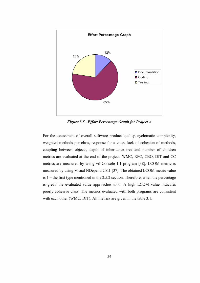
For the assessment of overall software product quality, cyclomatic complexity,

weighted methods per class, response for a class, lack of cohesion of methods,

coupling between objects, depth of inheritance tree and number of children

metrics are evaluated at the end of the project. WMC, RFC, CBO, DIT and CC

metrics are measured by using vil-Console 1.1 program [38]; LCOM metric is

measured by using Visual NDepend 2.8.1 [37]. The obtained LCOM metric value

is 1 – the first type mentioned in the 2.5.2 section. Therefore, when the percentage

is great, the evaluated value approaches to 0. A high LCOM value indicates

poorly cohesive class. The metrics evaluated with both programs are consistent

with each other (WMC, DIT). All metrics are given in the table 3.1.

35

Table 3.1 – Overall Quality Metrics of Project A

Class Name

Weighted Methods per Class

Response for Class

Lack of Cohesion of Methods

Coupling Between Objects

Depth in Tree

CombatMode 56 16 0.72 3 1

Communication 22 29 0.76 4 1

DataStorage 19 24 0.57 0 1

EthernetClient 22 29 0.83 1 2

MainGUI 47 84 0.93 2 7

Management 9 26 0.54 7 1

MessageOperations 9 11 NA 0 1

Missile 7 5 0 1 1

Seeker Head 3 4 0.33 0 1

SerialChannel 85 62 0.79 9 1

StandByMode 25 12 0.53 2 1

ULM 7 9 0.47 1 1

AVERAGE 25.92 28.27 0.59 2.73 1.73

Besides the given metrics in the table, NOC metric is measured at the end of the

project but NOC metric value for each class is 0. Thus, its value is not mentioned

in the above table. Method based evaluation is done for the CC metric and the

average of all methods has been calculated as 3,2. The maximum and minimum

values are also evaluated for each metric and displayed in Table 3.2.

Table 3.2 – Minimum and Maximum Values for the Product Metrics Evaluated

for Project A

WMC RFC LCOM CBO DIT CC

Minimum 3 4 0 0 1 1

Maximum 85 84 0,93 9 7 33

36

Requirement Phase

Design Phase

Coding

Testing

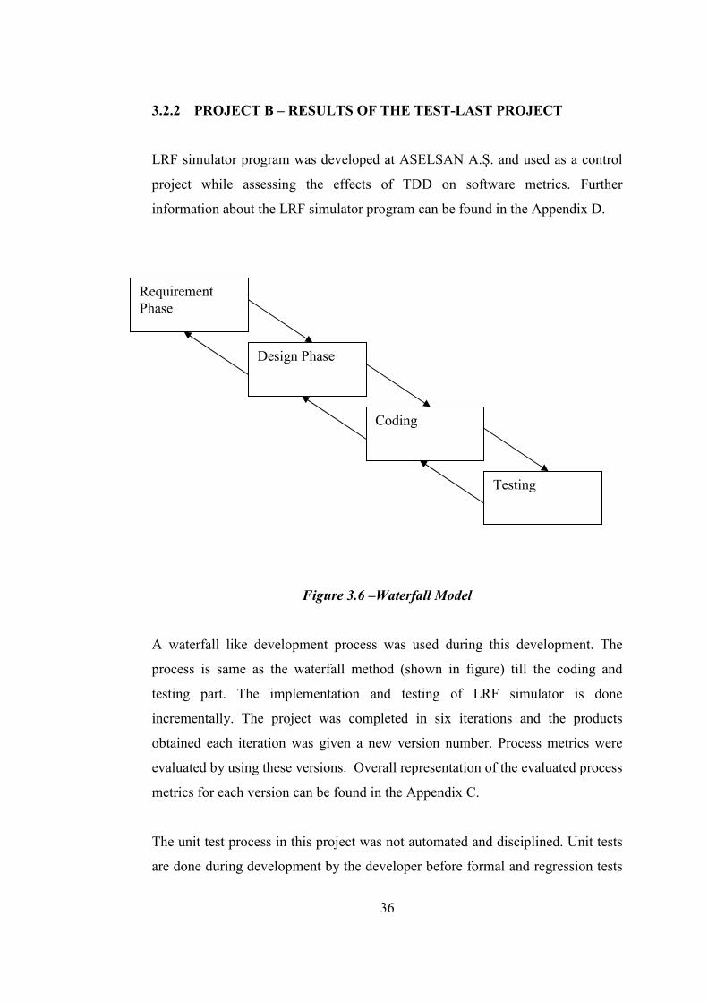
3.2.2 PROJECT B – RESULTS OF THE TEST-LAST PROJECT

LRF simulator program was developed at ASELSAN A.Ş. and used as a control

project while assessing the effects of TDD on software metrics. Further

information about the LRF simulator program can be found in the Appendix D.

Figure 3.6 –Waterfall Model

A waterfall like development process was used during this development. The

process is same as the waterfall method (shown in figure) till the coding and

testing part. The implementation and testing of LRF simulator is done

incrementally. The project was completed in six iterations and the products

obtained each iteration was given a new version number. Process metrics were

evaluated by using these versions. Overall representation of the evaluated process

metrics for each version can be found in the Appendix C.

The unit test process in this project was not automated and disciplined. Unit tests

are done during development by the developer before formal and regression tests

37

(tests that are held after each iteration). Small applications implemented or debug

prints were used for testing the methods and classes.

The iterations in the project were not planned so the work load was not separated

equally between them. In the first and the second iterations, the communication

base and the main GUI elements are implemented. Formal tests that are done with

a STD document were not held after these iterations; the defects were found by

the manual testing of the developer. The main functionality of the project was

implemented in the third and the fifth iterations and the tests were done with the

participation of customer after these steps. In the fourth and the sixth iterations,

the errors found in their previous increments, were corrected. Some missing new

functionality was also added in these iterations. Regression tests for the newly

added parts and the corrected parts were performed after these iterations.

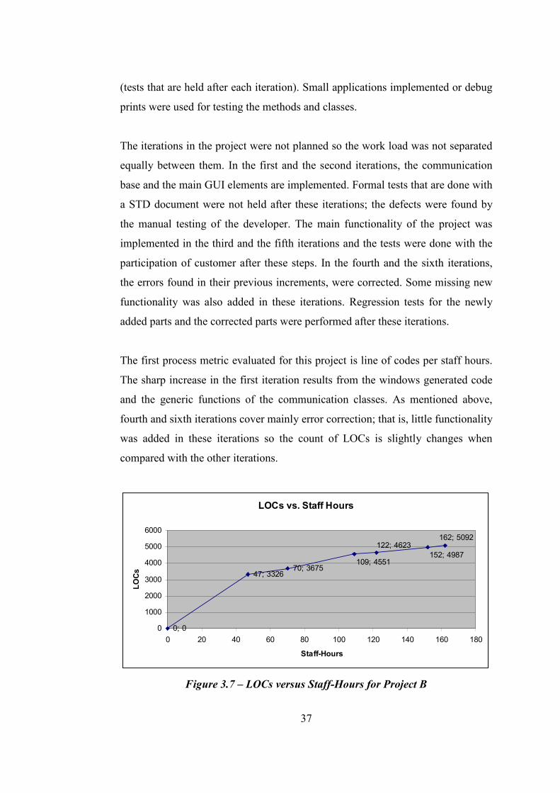
The first process metric evaluated for this project is line of codes per staff hours.

The sharp increase in the first iteration results from the windows generated code

and the generic functions of the communication classes. As mentioned above,

fourth and sixth iterations cover mainly error correction; that is, little functionality

was added in these iterations so the count of LOCs is slightly changes when

compared with the other iterations.

LOCs vs. Staff Hours

0; 0

47; 332670; 3675

162; 5092

152; 4987122; 4623

109; 4551

0

1000

2000

3000

4000

5000

6000

0 20 40 60 80 100 120 140 160 180

Staff-Hours

LOCs

Figure 3.7 – LOCs versus Staff-Hours for Project B

38

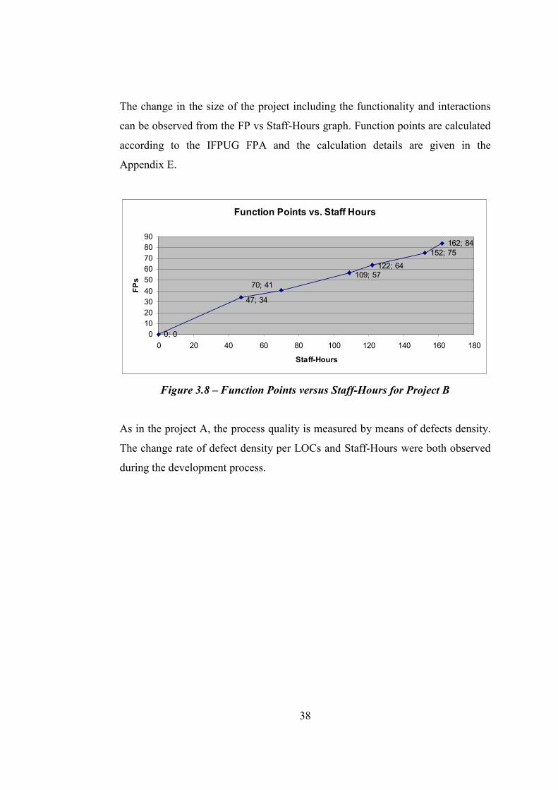
The change in the size of the project including the functionality and interactions

can be observed from the FP vs Staff-Hours graph. Function points are calculated

according to the IFPUG FPA and the calculation details are given in the

Appendix E.

Function Points vs. Staff Hours

0; 0

152; 75162; 84

47; 34

70; 41109; 57

122; 64

0

10

20

30

40

50

60

70

80

90

0 20 40 60 80 100 120 140 160 180

Staff-Hours

FPs

Figure 3.8 – Function Points versus Staff-Hours for Project B

As in the project A, the process quality is measured by means of defects density.

The change rate of defect density per LOCs and Staff-Hours were both observed

during the development process.

39

Defects Found vs. Staff Hours

0; 0

162; 22152; 21

122; 15

109; 13

70; 447; 2

0

5

10

15

20

25

0 20 40 60 80 100 120 140 160 180

Staff-Hours

# of Defects

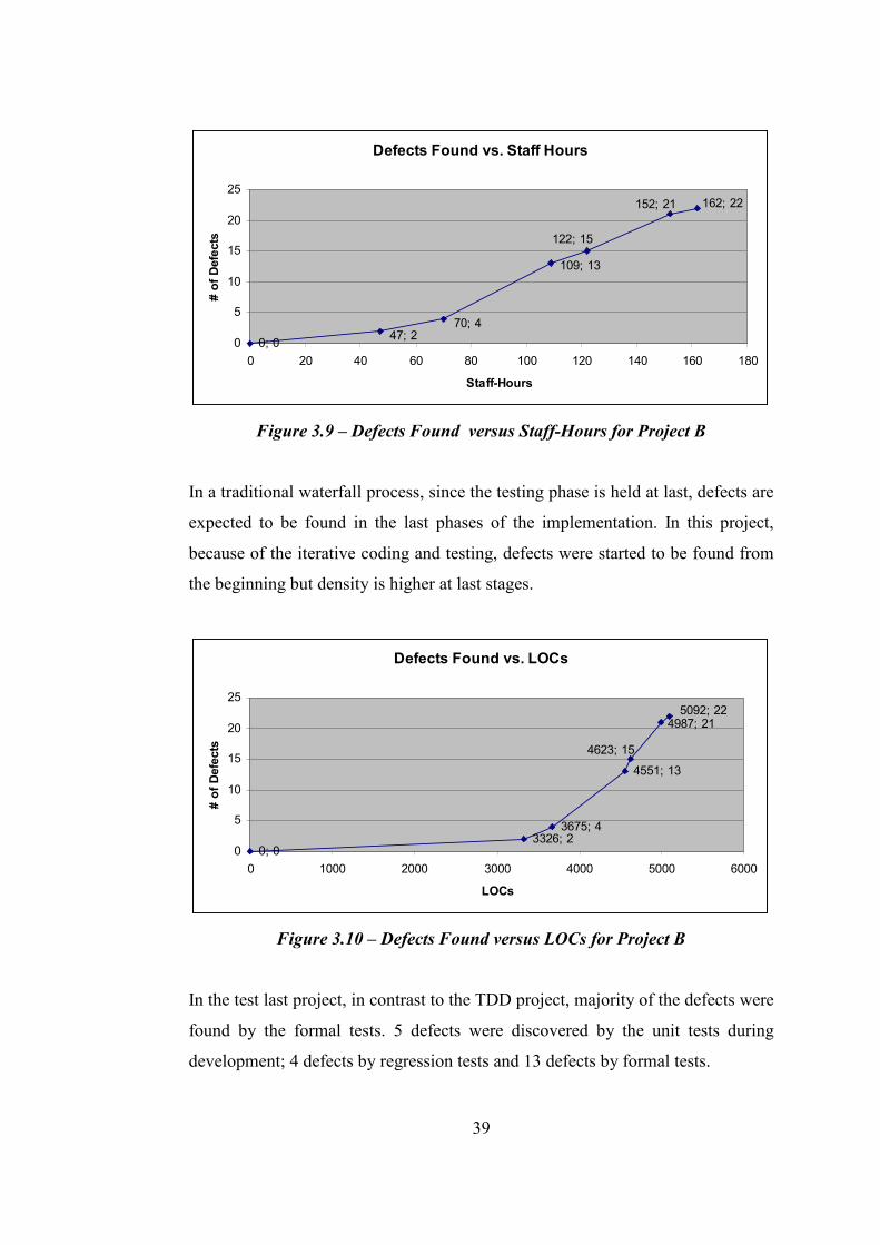
Figure 3.9 – Defects Found versus Staff-Hours for Project B

In a traditional waterfall process, since the testing phase is held at last, defects are

expected to be found in the last phases of the implementation. In this project,

because of the iterative coding and testing, defects were started to be found from

the beginning but density is higher at last stages.

Defects Found vs. LOCs

0; 03326; 2

3675; 4

4551; 13

4623; 15

4987; 215092; 22

0

5

10

15

20

25

0 1000 2000 3000 4000 5000 6000

LOCs

# of Defects

Figure 3.10 – Defects Found versus LOCs for Project B

In the test last project, in contrast to the TDD project, majority of the defects were

found by the formal tests. 5 defects were discovered by the unit tests during

development; 4 defects by regression tests and 13 defects by formal tests.

40

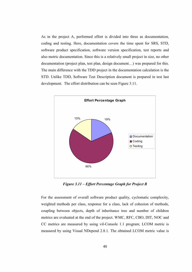
As in the project A, performed effort is divided into three as documentation,

coding and testing. Here, documentation covers the time spent for SRS, STD,

software product specification, software version specification, test reports and

also metric documentation. Since this is a relatively small project in size, no other

documentation (project plan, test plan, design document…) was prepared for this.

The main difference with the TDD project in the documentation calculation is the

STD. Unlike TDD, Software Test Description document is prepared in test last

development. The effort distribution can be seen Figure 3.11.

Effort Percentage Graph

19%

66%

15%

Documentation

Coding

Testing

Figure 3.11 – Effort Percentage Graph for Project B

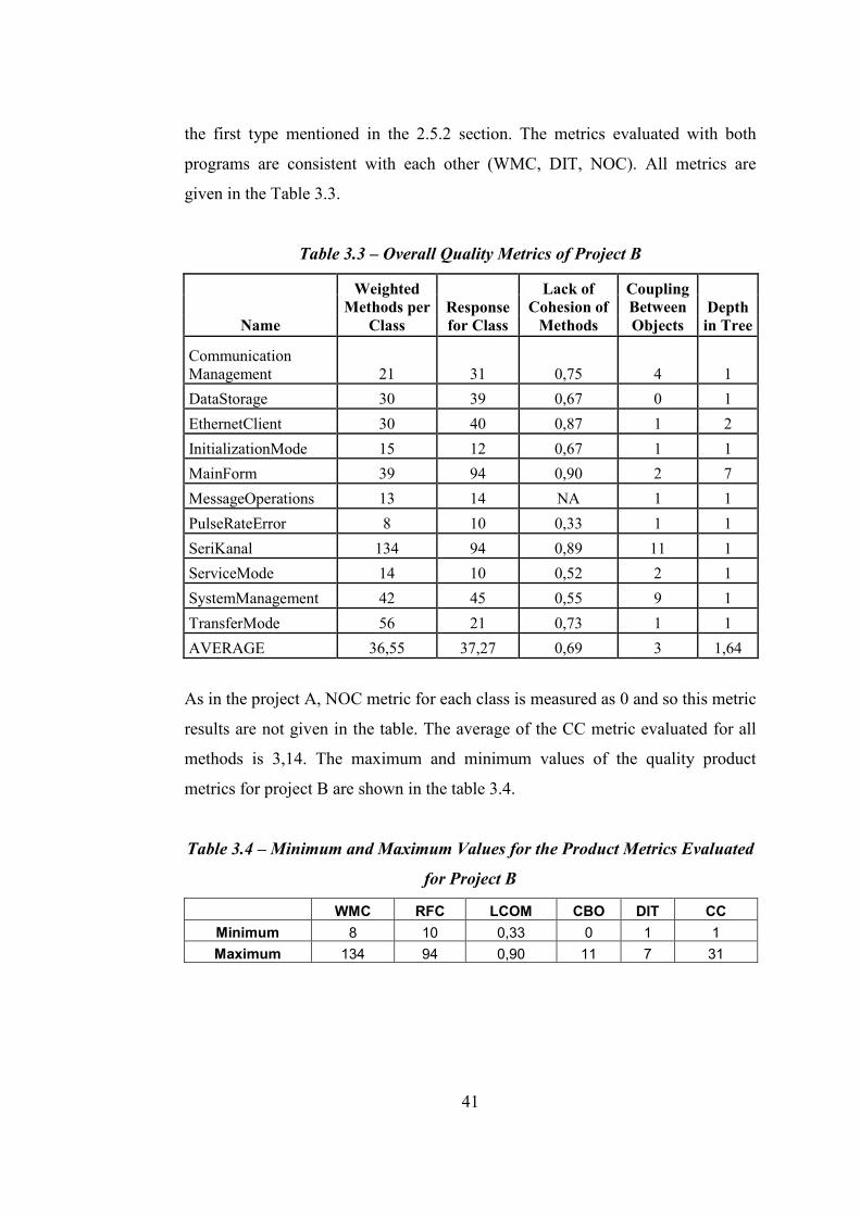
For the assessment of overall software product quality, cyclomatic complexity,

weighted methods per class, response for a class, lack of cohesion of methods,

coupling between objects, depth of inheritance tree and number of children

metrics are evaluated at the end of the project. WMC, RFC, CBO, DIT, NOC and

CC metrics are measured by using vil-Console 1.1 program; LCOM metric is

measured by using Visual NDepend 2.8.1. The obtained LCOM metric value is

41

the first type mentioned in the 2.5.2 section. The metrics evaluated with both

programs are consistent with each other (WMC, DIT, NOC). All metrics are

given in the Table 3.3.

Table 3.3 – Overall Quality Metrics of Project B

Name

Weighted Methods per

Class Response for Class

Lack of Cohesion of Methods

Coupling Between Objects

Depth in Tree

Communication Management 21 31 0,75 4 1

DataStorage 30 39 0,67 0 1

EthernetClient 30 40 0,87 1 2

InitializationMode 15 12 0,67 1 1

MainForm 39 94 0,90 2 7

MessageOperations 13 14 NA 1 1

PulseRateError 8 10 0,33 1 1

SeriKanal 134 94 0,89 11 1

ServiceMode 14 10 0,52 2 1

SystemManagement 42 45 0,55 9 1

TransferMode 56 21 0,73 1 1

AVERAGE 36,55 37,27 0,69 3 1,64

As in the project A, NOC metric for each class is measured as 0 and so this metric

results are not given in the table. The average of the CC metric evaluated for all

methods is 3,14. The maximum and minimum values of the quality product

metrics for project B are shown in the table 3.4.

Table 3.4 – Minimum and Maximum Values for the Product Metrics Evaluated

for Project B

WMC RFC LCOM CBO DIT CC

Minimum 8 10 0,33 0 1 1

Maximum 134 94 0,90 11 7 31

42

3.2.3 PROJECT C – EARLY WORK

Project C, namely SKN software, is developed using C# in Microsoft Visual

Studio .NET platform and working compatible with Microsoft Windows XP. The

project includes GUI classes and developed using waterfall development process.

Since SKN is a GUI application like the project A and also it is similar to TDD

project in terms of operating system and software language, a Test last – TDD

comparison between project A and C is performed within the scope of this thesis.

The final product of the project C is evaluated with object-oriented software

quality product metrics by using a free tool Visual NDepend 2.8.1.

SKN software is developed consistent with 249 software requirements. The

project is composed of 48 KLOCs so comparison of productivity becomes

meaningless. Besides GUI classes, SKN has two communication interfaces via

serial channel and also SKN projects includes database applications. SKN

software is composed of 80 classes and 46 of these classes are form classes. The

product metrics of all form classes are evaluated separately but Table 3.5, only

their averages are displayed.

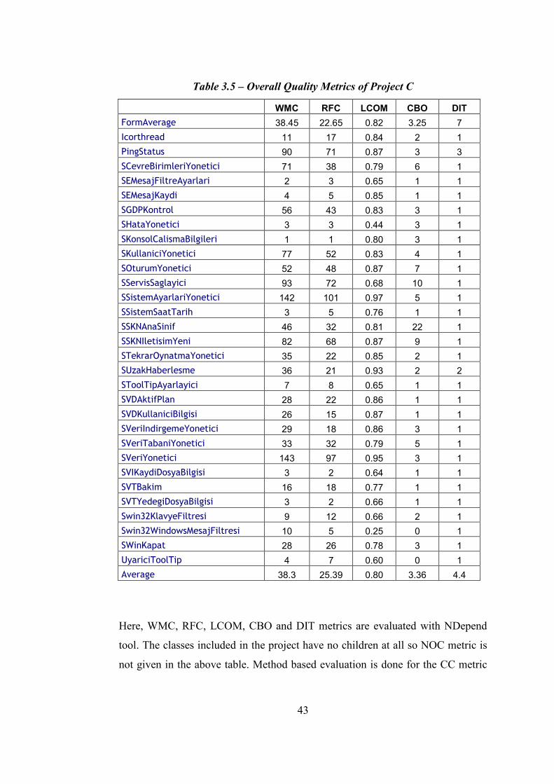
43

Table 3.5 – Overall Quality Metrics of Project C

WMC RFC LCOM CBO DIT

FormAverage 38.45 22.65 0.82 3.25 7

Icorthread 11 17 0.84 2 1

PingStatus 90 71 0.87 3 3

SCevreBirimleriYonetici 71 38 0.79 6 1

SEMesajFiltreAyarlari 2 3 0.65 1 1

SEMesajKaydi 4 5 0.85 1 1

SGDPKontrol 56 43 0.83 3 1

SHataYonetici 3 3 0.44 3 1

SKonsolCalismaBilgileri 1 1 0.80 3 1

SKullaniciYonetici 77 52 0.83 4 1

SOturumYonetici 52 48 0.87 7 1

SServisSaglayici 93 72 0.68 10 1

SSistemAyarlariYonetici 142 101 0.97 5 1

SSistemSaatTarih 3 5 0.76 1 1

SSKNAnaSinif 46 32 0.81 22 1

SSKNIletisimYeni 82 68 0.87 9 1

STekrarOynatmaYonetici 35 22 0.85 2 1

SUzakHaberlesme 36 21 0.93 2 2

SToolTipAyarlayici 7 8 0.65 1 1

SVDAktifPlan 28 22 0.86 1 1

SVDKullaniciBilgisi 26 15 0.87 1 1

SVeriIndirgemeYonetici 29 18 0.86 3 1

SVeriTabaniYonetici 33 32 0.79 5 1

SVeriYonetici 143 97 0.95 3 1

SVIKaydiDosyaBilgisi 3 2 0.64 1 1

SVTBakim 16 18 0.77 1 1

SVTYedegiDosyaBilgisi 3 2 0.66 1 1

Swin32KlavyeFiltresi 9 12 0.66 2 1

Swin32WindowsMesajFiltresi 10 5 0.25 0 1

SWinKapat 28 26 0.78 3 1

UyariciToolTip 4 7 0.60 0 1

Average 38.3 25.39 0.80 3.36 4.4

Here, WMC, RFC, LCOM, CBO and DIT metrics are evaluated with NDepend

tool. The classes included in the project have no children at all so NOC metric is

not given in the above table. Method based evaluation is done for the CC metric

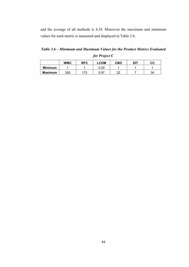
44

and the average of all methods is 4,18. Moreover the maximum and minimum

values for each metric is measured and displayed in Table 3.6.

Table 3.6 – Minimum and Maximum Values for the Product Metrics Evaluated

for Project C

WMC RFC LCOM CBO DIT CC

Minimum 1 1 0.25 1 1 1

Maximum 326 172 0.97 22 7 34

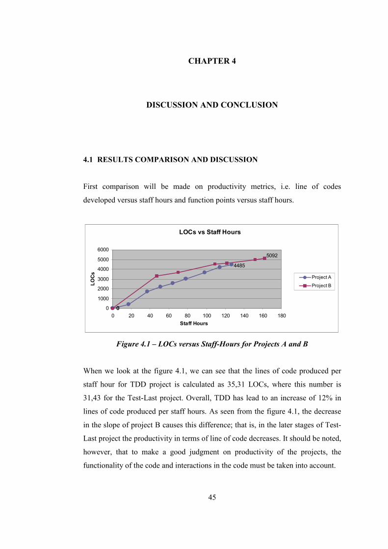
45

CHAPTER 4

DISCUSSION AND CONCLUSION

4.1 RESULTS COMPARISON AND DISCUSSION

First comparison will be made on productivity metrics, i.e. line of codes

developed versus staff hours and function points versus staff hours.

LOCs vs Staff Hours

00

4485

5092

0

1000

2000

3000

4000

5000

6000

0 20 40 60 80 100 120 140 160 180

Staff Hours

LOCs

Project A

Project B

Figure 4.1 – LOCs versus Staff-Hours for Projects A and B

When we look at the figure 4.1, we can see that the lines of code produced per

staff hour for TDD project is calculated as 35,31 LOCs, where this number is

31,43 for the Test-Last project. Overall, TDD has lead to an increase of 12% in

lines of code produced per staff hours. As seen from the figure 4.1, the decrease

in the slope of project B causes this difference; that is, in the later stages of Test-

Last project the productivity in terms of line of code decreases. It should be noted,

however, that to make a good judgment on productivity of the projects, the

functionality of the code and interactions in the code must be taken into account.

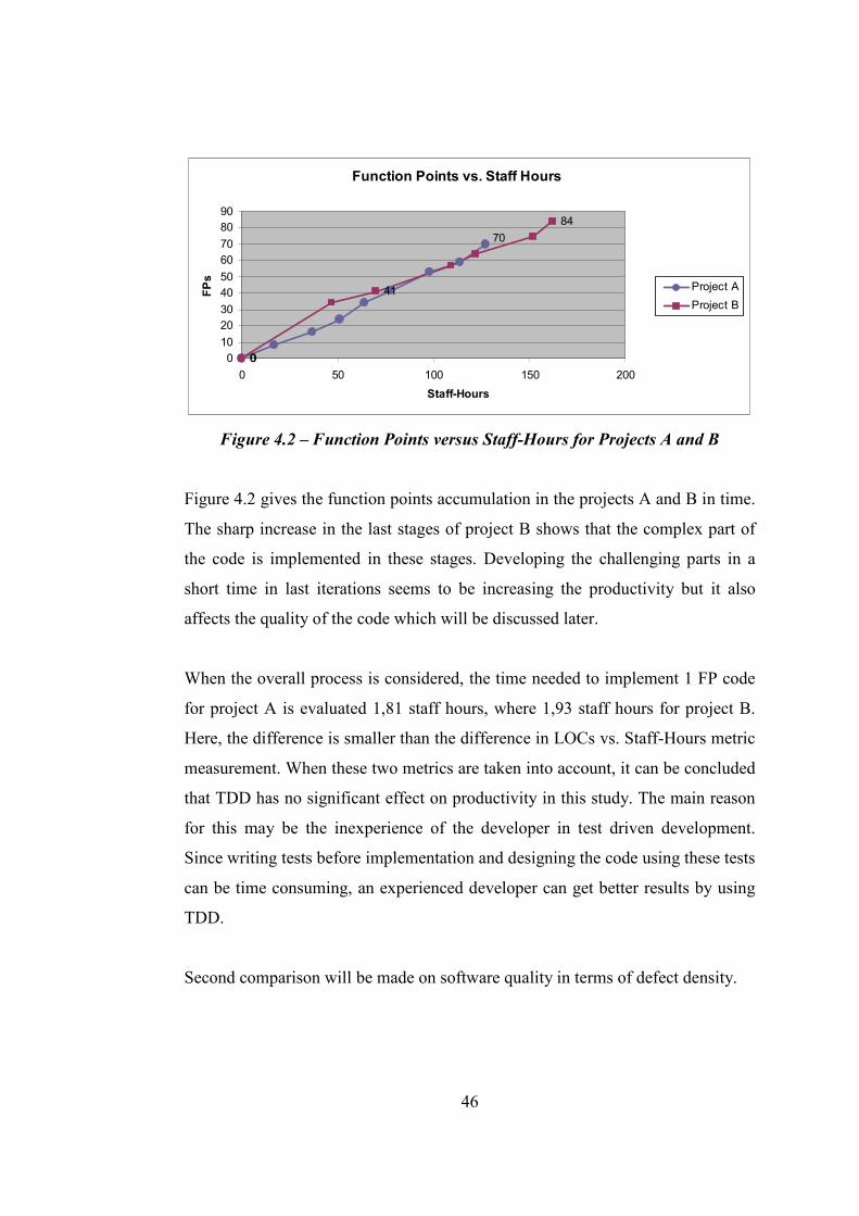
46

Function Points vs. Staff Hours

00

41

84

70

0

10

20

30

40

50

60

70

80

90

0 50 100 150 200

Staff-Hours

FPs

Project A

Project B

Figure 4.2 – Function Points versus Staff-Hours for Projects A and B

Figure 4.2 gives the function points accumulation in the projects A and B in time.

The sharp increase in the last stages of project B shows that the complex part of

the code is implemented in these stages. Developing the challenging parts in a

short time in last iterations seems to be increasing the productivity but it also

affects the quality of the code which will be discussed later.

When the overall process is considered, the time needed to implement 1 FP code

for project A is evaluated 1,81 staff hours, where 1,93 staff hours for project B.

Here, the difference is smaller than the difference in LOCs vs. Staff-Hours metric

measurement. When these two metrics are taken into account, it can be concluded

that TDD has no significant effect on productivity in this study. The main reason

for this may be the inexperience of the developer in test driven development.

Since writing tests before implementation and designing the code using these tests

can be time consuming, an experienced developer can get better results by using

TDD.

Second comparison will be made on software quality in terms of defect density.

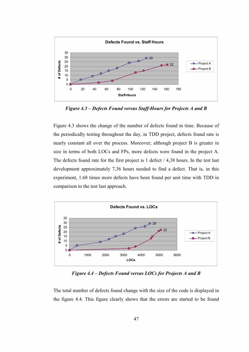
47

Defects Found vs. Staff Hours

29

22

0

510

1520

2530

35

0 20 40 60 80 100 120 140 160 180

Staff-Hours

# of Defects Project A

Project B

Figure 4.3 – Defects Found versus Staff-Hours for Projects A and B

Figure 4.3 shows the change of the number of defects found in time. Because of

the periodically testing throughout the day, in TDD project, defects found rate is

nearly constant all over the process. Moreover; although project B is greater in

size in terms of both LOCs and FPs, more defects were found in the project A.

The defects found rate for the first project is 1 defect / 4,38 hours. In the test last

development approximately 7,36 hours needed to find a defect. That is, in this

experiment, 1.68 times more defects have been found per unit time with TDD in

comparison to the test last approach.

Defects Found vs. LOCs

29

22

0

5

10

1520

25

30

35

0 1000 2000 3000 4000 5000 6000

LOCs

# of Defects

Project A

Project B

Figure 4.4 – Defects Found versus LOCs for Projects A and B

The total number of defects found change with the size of the code is displayed in

the figure 4.4. This figure clearly shows that the errors are started to be found

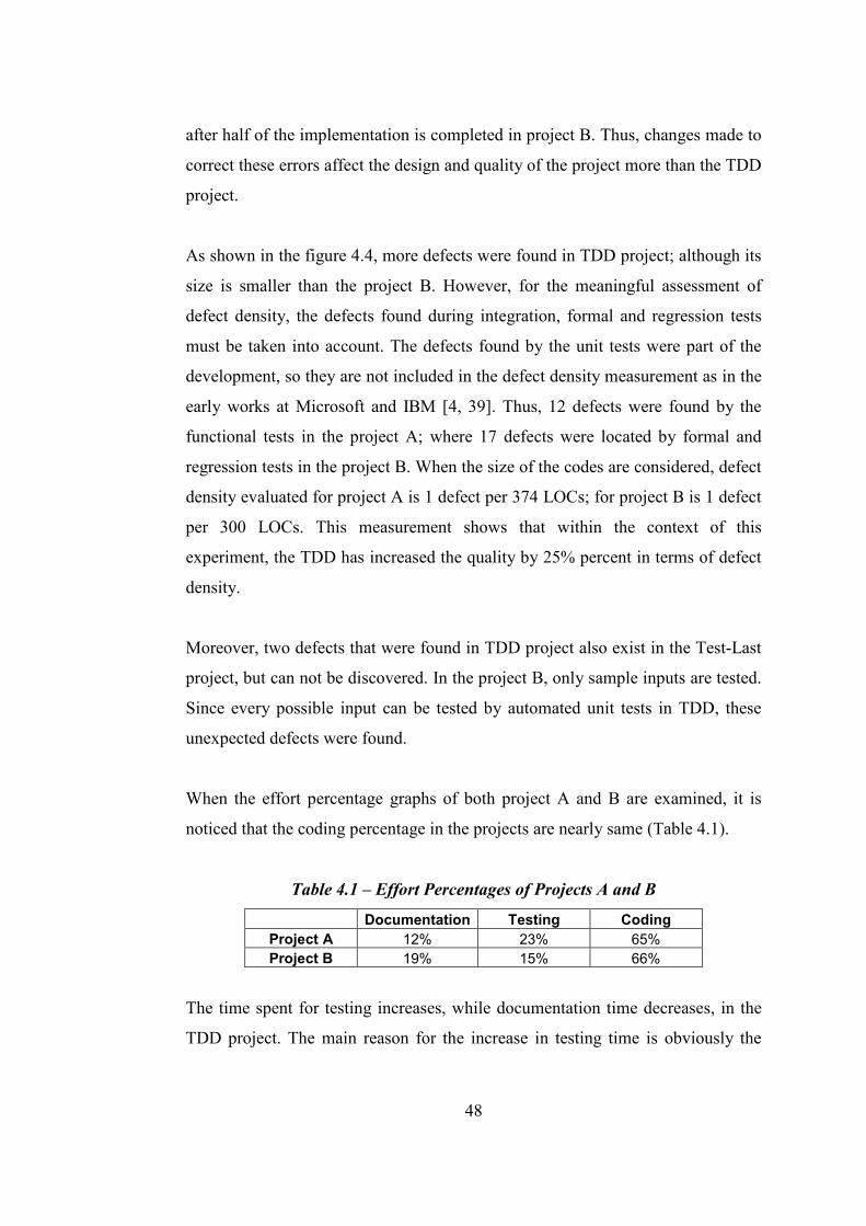
48

after half of the implementation is completed in project B. Thus, changes made to

correct these errors affect the design and quality of the project more than the TDD

project.

As shown in the figure 4.4, more defects were found in TDD project; although its

size is smaller than the project B. However, for the meaningful assessment of

defect density, the defects found during integration, formal and regression tests

must be taken into account. The defects found by the unit tests were part of the

development, so they are not included in the defect density measurement as in the

early works at Microsoft and IBM [4, 39]. Thus, 12 defects were found by the

functional tests in the project A; where 17 defects were located by formal and

regression tests in the project B. When the size of the codes are considered, defect

density evaluated for project A is 1 defect per 374 LOCs; for project B is 1 defect

per 300 LOCs. This measurement shows that within the context of this

experiment, the TDD has increased the quality by 25% percent in terms of defect

density.

Moreover, two defects that were found in TDD project also exist in the Test-Last

project, but can not be discovered. In the project B, only sample inputs are tested.

Since every possible input can be tested by automated unit tests in TDD, these

unexpected defects were found.

When the effort percentage graphs of both project A and B are examined, it is

noticed that the coding percentage in the projects are nearly same (Table 4.1).

Table 4.1 – Effort Percentages of Projects A and B

Documentation Testing Coding

Project A 12% 23% 65% Project B 19% 15% 66%

The time spent for testing increases, while documentation time decreases, in the

TDD project. The main reason for the increase in testing time is obviously the

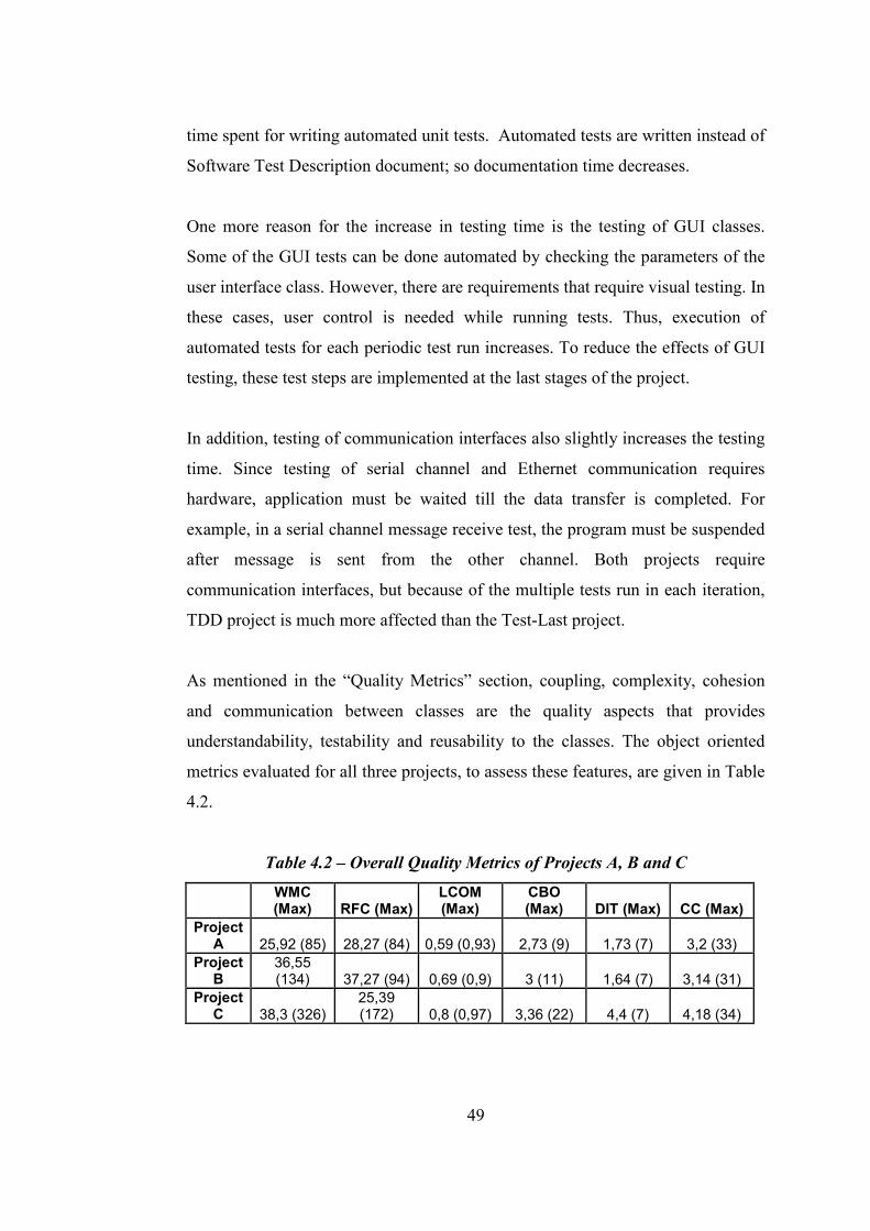
49

time spent for writing automated unit tests. Automated tests are written instead of

Software Test Description document; so documentation time decreases.

One more reason for the increase in testing time is the testing of GUI classes.

Some of the GUI tests can be done automated by checking the parameters of the

user interface class. However, there are requirements that require visual testing. In

these cases, user control is needed while running tests. Thus, execution of

automated tests for each periodic test run increases. To reduce the effects of GUI

testing, these test steps are implemented at the last stages of the project.

In addition, testing of communication interfaces also slightly increases the testing

time. Since testing of serial channel and Ethernet communication requires

hardware, application must be waited till the data transfer is completed. For

example, in a serial channel message receive test, the program must be suspended

after message is sent from the other channel. Both projects require

communication interfaces, but because of the multiple tests run in each iteration,

TDD project is much more affected than the Test-Last project.

As mentioned in the “Quality Metrics” section, coupling, complexity, cohesion

and communication between classes are the quality aspects that provides

understandability, testability and reusability to the classes. The object oriented

metrics evaluated for all three projects, to assess these features, are given in Table

4.2.

Table 4.2 – Overall Quality Metrics of Projects A, B and C

WMC (Max) RFC (Max)

LCOM (Max)

CBO (Max) DIT (Max) CC (Max)

Project A 25,92 (85) 28,27 (84) 0,59 (0,93) 2,73 (9) 1,73 (7) 3,2 (33)

Project B

36,55 (134) 37,27 (94) 0,69 (0,9) 3 (11) 1,64 (7) 3,14 (31)

Project C 38,3 (326)

25,39 (172) 0,8 (0,97) 3,36 (22) 4,4 (7) 4,18 (34)

50

Weighted methods per class metric is lower in TDD project than the other

projects. This makes projects B and C hard to test, less understandable and less

reusable. FormSKNAna class in project C has a very high WMC value and also

RFC and LCOM values which show that the class is not understandable and must

be divided. Moreover, when project A and B’s metrics are examined, it is

observed that the maximum WMC valued classes are the classes with similar

responsibilities. Both of the classes were implemented to provide serial channel

connection and message transfer using serial channel. In TDD project, the

irrelevant parts, which were not noticed during test last development, were not

implemented. As a result, the code size decreases and the quality increases in

TDD; but functionality is still the same.

RFC metric measures the communication density between the methods of the

classes. As in the WMC metric result, RFC value of project A is lower than the

test last project; but, a little higher than the early work average. This makes

testing and debugging harder for project B.

For LCOM metric, the values greater than 0,8 point lack of cohesion [37].

Although MainGUI class of project A has a LCOM value of 0,93, TDD project’s

classes are more cohesive than the others. In project B, poorly cohesive classes

are GUI class and communication classes. The connection of communication

classes with lower layers may lead to increase in cohesion, but the similar classes

in project A have lower LCOM values. Exclusion of irrelevant parts from the

code increases cohesiveness of the classes. In project C, half of the classes are not

cohesive enough and need to be splited to increase cohesion.

There is no significant difference between CBO values of the projects. TDD

project has low coupling than the others on the average.

Larger DIT values make classes less understandable; on the contrary larger DIT

values indicate potential for reuse of inherited methods. When DIT values of

51

project A and B are examined, no effect of TDD on depth of inheritance can be

seen. DIT value in project is great because 46 of 80 classes included in project C

are form classes which has a DIT value of 7.

Control flow complexity is evaluated with cyclomatic complexity metric.

Average CC of methods of projects A and B are nearly same. Project C has a

greater average complexity which can be caused from the larger size of the

project.

4.2 CONCLUSION

In this study, a software project was developed using test driven development

technique and compared in terms of software productivity and software quality

with two software projects developed using the traditional Test-Last technique.

Both process and the final product comparisons are made by measuring relevant

software metrics. Furthermore, throughout the development process, benefits and

challenges of TDD are also examined.

There were contradicting results in the literature about the effects of TDD to

developers’ productivity. In our study, productivity is measured by calculating the

change of size with the time. Obtained results given in the previous section show

that, in the context of the experiment performed, the effect of TDD on

productivity was insignificant. It should, however, be mentioned that the

unfamiliarity of the developer with TDD may have caused this outcome.

Quality assessment of the projects is achieved by measuring seven product quality

metrics and also by examining the change of the total number of defects found

with both size and time. The defects found during unit tests are considered as the

part of development so they are excluded in defect density calculation. By

observing the results, it can be concluded that the quality is improved in TDD

52

project in terms of class complexity and defect density. It is observed that more

cohesive and less complex classes are obtained by using TDD technique. Since

defects are found at the later stages of the project, the architecture of the code is

much more corrupted in the Test-Last approach. In fact, the higher defect density

values measured in the Test-Last project may, in turn, be a result of complexity

and lack of cohesive classes.

On the other hand, again, in the context of this experiment, the test driven

technique has had a little positive effect on coupling. The developed projects

consist of few classes and so, small coupling values are observed. Coupling

comparison in larger projects may give more meaningful results. Similarly, effect

of TDD on inheritance could not be observed in this study. There was no need for

inheritance usage in the developed projects and depth of inheritance values are

constituted by the form classes.

As mentioned in Chapter 2, there seems to be a consensus in the literature on the

fact that using test driven development in projects involving network

communication and GUI has some challenges. Both challenges lead to an increase

in testing time. The results of this increase were not serious in this study; mainly

high testing duration was caused by the automated unit tests. However, network

testing and GUI testing may lead to devastating delays in projects including more

complicated networks and too many GUI classes.

Further work in this area may consist of studies on projects in different domains,

and projects with a wide range of sizes. A limitation of the current experiment

was that only three projects were compared. If the aim of establishing a definitive

assessment of TDD on productivity and product quality is adopted, much more

extensive studies in terms of software types, including a diversity of domains,

software sizes and also organization sizes and characteristics such as development

maturity, as assessed by techniques such as CMMI, must be considered.

53

REFERENCES

[1] A. Geras, M. Smith and J. Miller, A Prototype Empirical Evaluation of

Test Driven Development, Proceedings of the 10th International Symposium on

Software Metrics (METRICS’04), 2004, pp. 405 – 416.

[2] K. Beck, Test Driven Development by Example, Addison-Wesley, 2003.

[3] D. Astels, Test Driven Development A Practical Guide, Prentice Hall,

2003, pp. 5 -15.

[4] T. Bhat and N. Nagappan, Evaluating the Efficacy of Test-Driven

Development: Industrial Case Studies, Proceedings of the 2006 ACM/IEEE

international symposium on International symposium on empirical software

engineering, Rio de Janeiro, Brazil, 2006, pp. 356 – 363.

[5] H. Erdogmus, M. Morisio and M. Torchiano, On the Effectiveness of the

Test-First Approach to Programming, IEEE Transactions in Software Engineering

31(3), 2005, pp. 226 – 237.

[6] E. M. Maximilien and L. Williams, Assessing Test-Driven Development

at IBM, Proceedings of the 25th International Conference on Software

Engineering (ICSE’03), 2003, pp. 564 – 569.

[7] H. Ryu, B. Sohn and J. Park, Mock Objects Framework for TDD in the

Network Environment, Proceedings of the Fourth Annual ACIS International

Conference on Computer and Information Science (ICIS’05), 2005, pp. 430 –

434.

54

[8] M. J. Karlesky, W. I. Bereza and C. B. Erickson, Effective Test Driven

Development for Embedded Software, IEEE 2006 Electro/Information

Technology Conference Michigan State University, May 2006, pp. 382 – 387.

[9] M. Alles, D. Crosby, C. Erickson, B. Harleton, M. Marsiglia, G. Pattison,

and C. Stienstra, Presenter First: Organizing Complex GUI Applications for Test-

Driven Development, Proceedings of AGILE 2006 Conference(AGILE’06),

2006, p. 10.

[10] D. S. Janzen, Software architecture improvement through test-driven

development, Companion to the 20th annual ACM SIGPLAN conference on

Object-oriented programming, systems, languages, and applications San Diego,

CA, USA, October 16-20, 2005, pp. 240 – 241.

[11] L. C. Briand, J. Daly, V. Porter and J. Wüst, A Comprehensive Empirical

Validation of Design Measures for Object-Oriented Systems, Proceedings of the

Fifth International Symposium on Software Metrics, November 1998, p. 246.

[12] D. Janzen and H. Saiedian, On the influence of test-driven development on

software design, Proceedings of the 19th Conference on Software Engineering

Education & Training, 2006, pp. 141 – 148.

[13] K. E. Wiegers, A Software Metrics Primer, Software Development

magazine, July 1999, pages 12, 13 and 16.

[14] IEEE Standart for Software Productivity Metrics, IEEE Std 1045-1992.

[15] A. J. Albrecht, Measuring Application Development Productivity, IBM

Applications Development Symposium, Monterey, CA, 1979, pp. 83 – 92.

55

[16] IEEE Standart for Software Quality Metrics, IEEE Std 1061-1998

(R2004).

[17] Y. K. Malaiya and J. Denton, Module Size Distribution and Defect

Density, Proceedings of the 11th International Symposium on Software

Reliability Engineering, 2000, p. 62.

[18] Software Assurance Technology Center (SATC), Software Quality

Metrics, June 1995.

[19] J. Lindroos, Code and Design Metrics for Object-Oriented Systems,

Seminar on Quality Models for Software Engineering, University of Helsinki,

December 2004.

[20] C. Jones, Strengths and Weakness of Software Metrics, Chief Scientist

Emeritus, Software Productivity Research LLC, March 22, 2006.

[21] D. Pace, G. Calavaro and G. Cantone, Function Point and UML: State of

the Art and Evaluation Model, Proceedings of SMEF04, Roma, June, 2004.

[22] D. St-Pierre, M. Maya, A. Abran, J-M. Desharnais and P. Bourque, “Full

Function Points: Counting Practices Manual”, Technical Report 1997-04,

Software Engineering Management Research Laboratory and Software

Engineering Laboratory in Applied Metrics (SELAM), 1997.

[23] B. Henderson-Sellers, OO Software Process Improvement with Metrics,

Proceedings of the Software Metrics Symposium, 1999, pp. 2 – 8.

[24] W. Li, Software Product Metrics, IEEE Potentials, Volume 18, Issue 5,

Dec. 1999 – Jan. 2000, pp. 24 – 27.

56

[25] H. Smith and P. Fingar, Business Process Management: The Third Wave,

March/April, 2001.

[26] R. Xu, Y. Xue, P. Nie, Y. Zhang and D. Li, Research on CMMI-based

Software Process Metrics, Proceedings of the First International Multi-

Symposiums on Computer and Computational Sciences (IMSCCS'06), 2006, pp.

391 – 397.

[27] S. Hayes and M. Andrews, An Introduction to Agile Methods, Retrieved

June 18th, 2007 from

http://www.wrytradesman.com/articles/IntroToAgileMethods.pdf, 2000.

[28] K. Beck, M. Beedle, A. van Bennekum, A. Cockburn, W. Cunningham,

M. Fowler, J. Grenning, J. Highsmith, A. Hunt, R. Jeffries, J. Kern, B. Marick, R.

C. Martin, S. Mellor, K. Schwaber, J. Sutherland, and D. Thomas, Manifesto for

Agile Software Development, 2007 retrieved from http://AgileManifesto.org.

[29] L. Williams, A Survey of Agile Development Methodologies, Retrieved

June 17th, 2007 from http://agile.csc.ncsu.edu/SEMaterials/AgileMethods.pdf,

2004.

[30] C. Gencel, An Architectural Dimensions Based Software Functional Size

Measurement Method, A Thesis Submitted to the Graduate School of Informatics

of the Middle East Technical University, July 2005.

[31] C. Gencel, O. Demirors and E. Yuceer, Utilizing Functional Size

Measurement Methods for Real Time Software Systems, Program of Metrics,

September 2005.

57

[32] B. Aydınoz, The Effect of Design Patterns on Object-Oriented Metrics and

Software Error-Pronenses, A Thesis Submitted to the Graduate School of Natural

and Applied Sciences of the Middle East Technical University, September 2006.

[33] S. Chidamber and C. Kemerer, A Metrics Suite for Object-Oriented

Design, IEEE Transactions on Software Engineering, Vol. 20, No. 6, June 1994,

pp. 476 – 493.

[34] V. R. Basili, L. C. Briand and W. L. Melo, A Validation of Object-

Oriented Design Metrics as Quality Indicators, IEEE Transactions on Software

Engineering, Vol. 20, No. 10, October 1996, pp. 751 – 761.

[35] Extreme Programming, 2008 retrieved from

http://www.extremeprogramming.org/.

[36] NUnit, 2008 retrieved from http://www.nunit.org.

[37] NDepend, 2008 retrieved from http://www.ndepend.com/.

[38] Vil - Console, 2008 retrieved from http://www.1bot.com/.

[39] L. Williams, E. M. Maximilien and M. Vouk, Test-Driven Development

as a Defect-Reduction Practice, Proceedings of IEEE International Symposium on

Software Reliability Engineering, Denver, 2003, pp. 34 – 45.

[40] C. R. Symons, Function Point Analysis: Difficulties and Improvements,

IEEE Transactions on Software Engineering, Vol. 14 No. 1, January 1988, pp. 2 –

11.

[41] United Kingdom Software Metrics Association (UKSMA), MK II

Function Point Analysis Counting Practices Manual Version 1.3.1., 1998.

58

[42] A. Abran, COSMIC FFP 2.0: An Implementation of COSMIC Functional

Size Measurement Concepts, FESMA’99, Amsterdam, 7 October 1999.

[43] The Common Software Measurement International Consortium

(COSMIC), FFP, version 3.0, Measurement Manual, September 2007.

[44] The International Function Point Users Group, Function Point Counting

Practices Manual - Release. 4.1, 1999.

[45] A. J. Albrecht and J. E. Gaffney, Software Function, Source Lines of

Code, and Development Effort Prediction: A Software Science Validation, IEEE

Transactions on Software Engineering, Vol. SE-9, No. 6, November 1983, pp.

639 – 648.

[46] The Netherlands Software Metric Association, 2008 retrieved from

http://www.nesma.nl/.

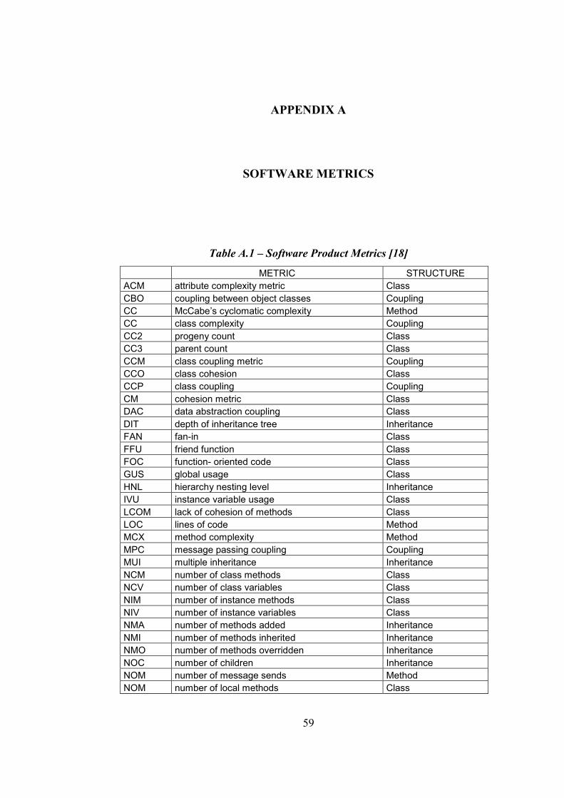
59

APPENDIX A

SOFTWARE METRICS

Table A.1 – Software Product Metrics [18]

METRIC STRUCTURE ACM attribute complexity metric Class CBO coupling between object classes Coupling CC McCabe’s cyclomatic complexity Method CC class complexity Coupling CC2 progeny count Class CC3 parent count Class CCM class coupling metric Coupling CCO class cohesion Class CCP class coupling Coupling CM cohesion metric Class DAC data abstraction coupling Class DIT depth of inheritance tree Inheritance FAN fan-in Class FFU friend function Class FOC function- oriented code Class GUS global usage Class HNL hierarchy nesting level Inheritance IVU instance variable usage Class LCOM lack of cohesion of methods Class LOC lines of code Method MCX method complexity Method MPC message passing coupling Coupling MUI multiple inheritance Inheritance NCM number of class methods Class NCV number of class variables Class NIM number of instance methods Class NIV number of instance variables Class NMA number of methods added Inheritance NMI number of methods inherited Inheritance NMO number of methods overridden Inheritance NOC number of children Inheritance NOM number of message sends Method NOM number of local methods Class

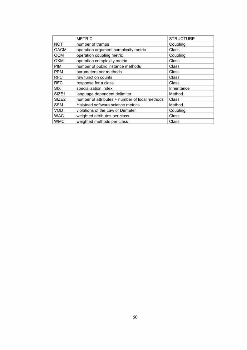
60

METRIC STRUCTURE NOT number of tramps Coupling OACM operation argument complexity metric Class OCM operation coupling metric Coupling OXM operation complexity metric Class PIM number of public instance methods Class PPM parameters per methods Class RFC raw function counts Class RFC response for a class Class SIX specialization index Inheritance SIZE1 language dependent delimiter Method SIZE2 number of attributes + number of local methods Class SSM Halstead software science metrics Method VOD violations of the Law of Demeter Coupling WAC weighted attributes per class Class WMC weighted methods per class Class

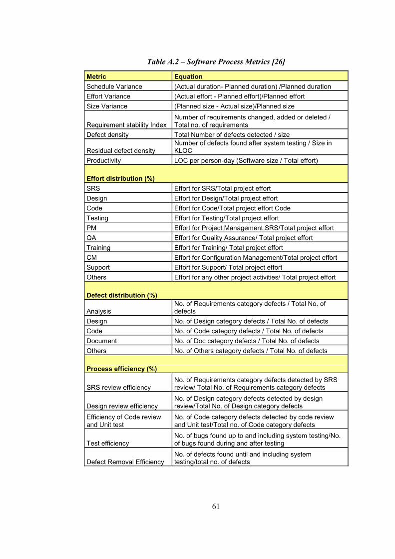
61

Table A.2 – Software Process Metrics [26]

Metric Equation

Schedule Variance (Actual duration- Planned duration) /Planned duration

Effort Variance (Actual effort - Planned effort)/Planned effort

Size Variance (Planned size - Actual size)/Planned size

Requirement stability Index Number of requirements changed, added or deleted / Total no. of requirements

Defect density Total Number of defects detected / size

Residual defect density Number of defects found after system testing / Size in KLOC

Productivity LOC per person-day (Software size / Total effort)

Effort distribution (%)

SRS Effort for SRS/Total project effort

Design Effort for Design/Total project effort

Code Effort for Code/Total project effort Code

Testing Effort for Testing/Total project effort

PM Effort for Project Management SRS/Total project effort

QA Effort for Quality Assurance/ Total project effort

Training Effort for Training/ Total project effort

CM Effort for Configuration Management/Total project effort

Support Effort for Support/ Total project effort

Others Effort for any other project activities/ Total project effort

Defect distribution (%)

Analysis No. of Requirements category defects / Total No. of defects

Design No. of Design category defects / Total No. of defects

Code No. of Code category defects / Total No. of defects

Document No. of Doc category defects / Total No. of defects

Others No. of Others category defects / Total No. of defects

Process efficiency (%)

SRS review efficiency No. of Requirements category defects detected by SRS review/ Total No. of Requirements category defects

Design review efficiency No. of Design category defects detected by design review/Total No. of Design category defects

Efficiency of Code review and Unit test

No. of Code category defects detected by code review and Unit test/Total no. of Code category defects

Test efficiency No. of bugs found up to and including system testing/No. of bugs found during and after testing

Defect Removal Efficiency No. of defects found until and including system testing/total no. of defects

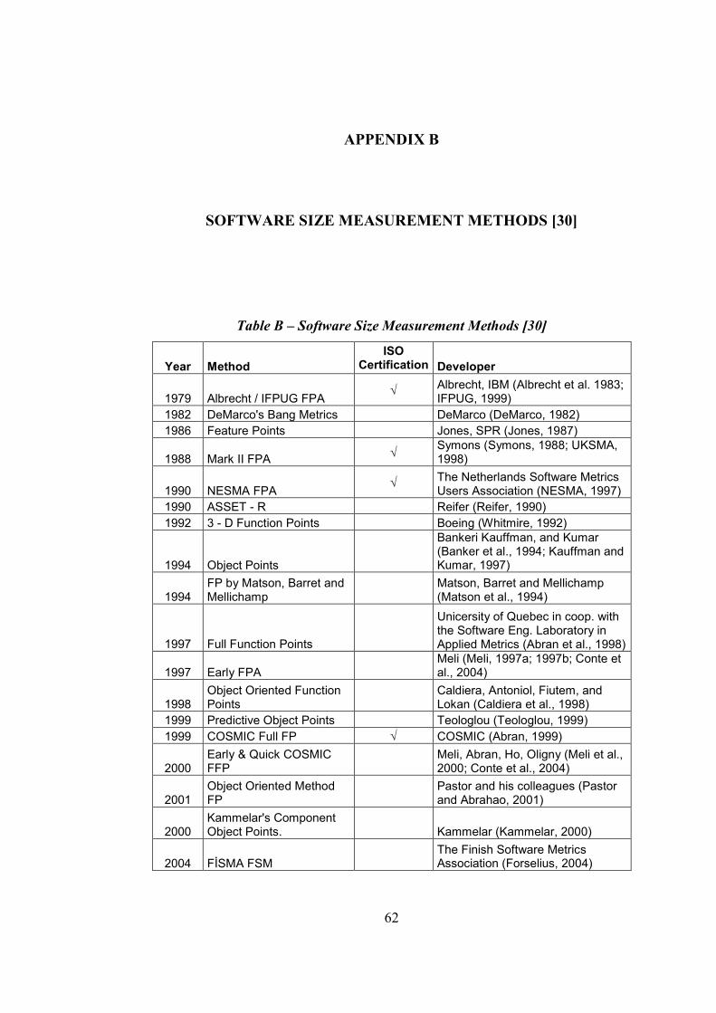
62

APPENDIX B

SOFTWARE SIZE MEASUREMENT METHODS [30]

Table B – Software Size Measurement Methods [30]

Year Method

ISO Certification Developer

1979 Albrecht / IFPUG FPA √

Albrecht, IBM (Albrecht et al. 1983; IFPUG, 1999)

1982 DeMarco's Bang Metrics DeMarco (DeMarco, 1982) 1986 Feature Points Jones, SPR (Jones, 1987)

1988 Mark II FPA √ Symons (Symons, 1988; UKSMA, 1998)

1990 NESMA FPA √

The Netherlands Software Metrics Users Association (NESMA, 1997)

1990 ASSET - R Reifer (Reifer, 1990)

1992 3 - D Function Points Boeing (Whitmire, 1992)

1994 Object Points

Bankeri Kauffman, and Kumar (Banker et al., 1994; Kauffman and Kumar, 1997)

1994 FP by Matson, Barret and Mellichamp

Matson, Barret and Mellichamp (Matson et al., 1994)

1997 Full Function Points

Unicersity of Quebec in coop. with the Software Eng. Laboratory in Applied Metrics (Abran et al., 1998)

1997 Early FPA

Meli (Meli, 1997a; 1997b; Conte et al., 2004)

1998 Object Oriented Function Points

Caldiera, Antoniol, Fiutem, and Lokan (Caldiera et al., 1998)

1999 Predictive Object Points Teologlou (Teologlou, 1999)

1999 COSMIC Full FP √ COSMIC (Abran, 1999)

2000 Early & Quick COSMIC FFP

Meli, Abran, Ho, Oligny (Meli et al., 2000; Conte et al., 2004)

2001 Object Oriented Method FP

Pastor and his colleagues (Pastor and Abrahao, 2001)

2000 Kammelar's Component Object Points.

Kammelar (Kammelar, 2000)

2004 FĐSMA FSM The Finish Software Metrics

Association (Forselius, 2004)

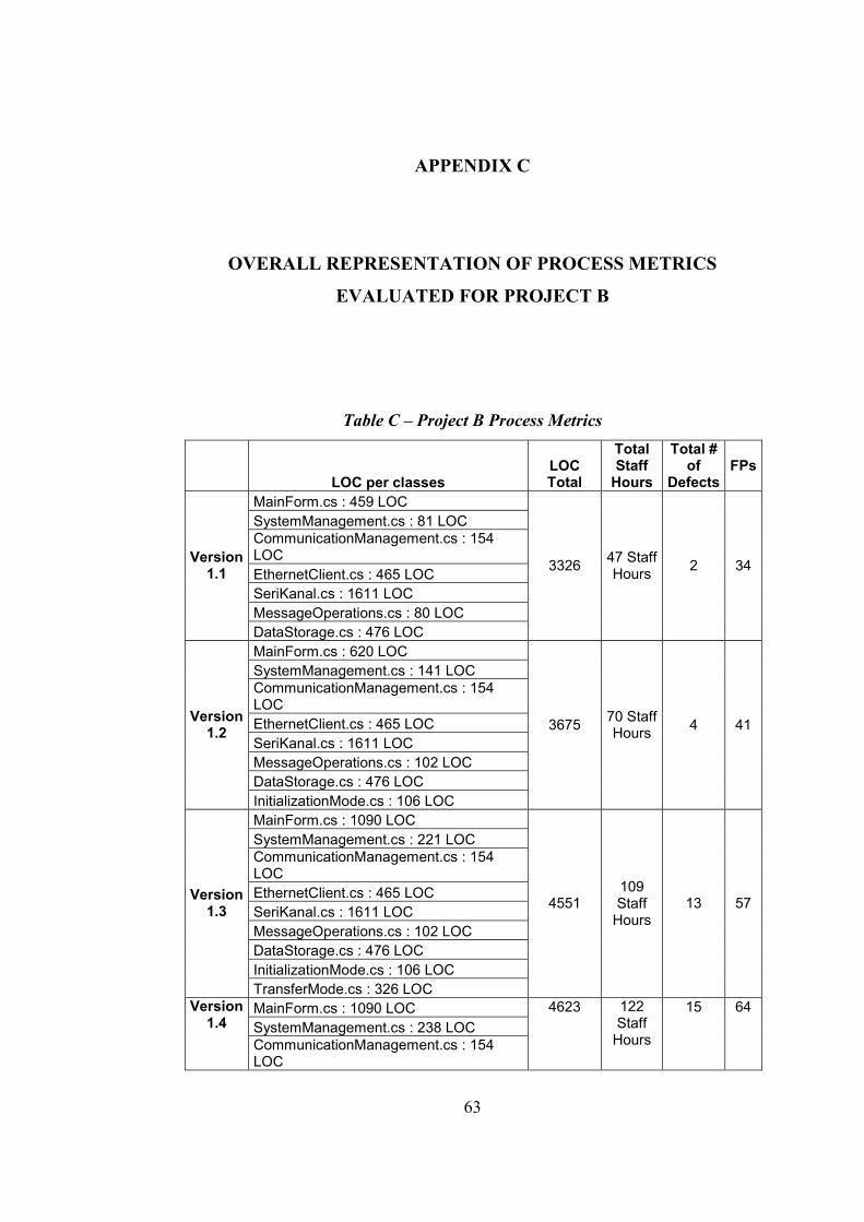
63

APPENDIX C

OVERALL REPRESENTATION OF PROCESS METRICS

EVALUATED FOR PROJECT B

Table C – Project B Process Metrics

LOC per classes LOC Total

Total Staff Hours

Total # of

Defects

FPs

MainForm.cs : 459 LOC SystemManagement.cs : 81 LOC CommunicationManagement.cs : 154 LOC EthernetClient.cs : 465 LOC SeriKanal.cs : 1611 LOC MessageOperations.cs : 80 LOC

Version 1.1

DataStorage.cs : 476 LOC

3326 47 Staff Hours

2 34

MainForm.cs : 620 LOC SystemManagement.cs : 141 LOC CommunicationManagement.cs : 154 LOC EthernetClient.cs : 465 LOC SeriKanal.cs : 1611 LOC MessageOperations.cs : 102 LOC DataStorage.cs : 476 LOC

Version 1.2

InitializationMode.cs : 106 LOC

3675 70 Staff Hours

4 41

MainForm.cs : 1090 LOC SystemManagement.cs : 221 LOC CommunicationManagement.cs : 154 LOC EthernetClient.cs : 465 LOC SeriKanal.cs : 1611 LOC MessageOperations.cs : 102 LOC DataStorage.cs : 476 LOC InitializationMode.cs : 106 LOC

Version 1.3

TransferMode.cs : 326 LOC

4551 109 Staff Hours

13 57

MainForm.cs : 1090 LOC SystemManagement.cs : 238 LOC

Version 1.4

CommunicationManagement.cs : 154 LOC

4623 122 Staff Hours

15 64

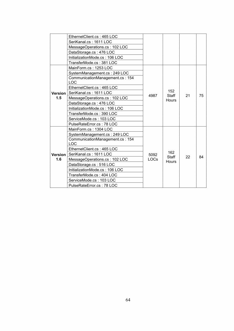
64

EthernetClient.cs : 465 LOC SeriKanal.cs : 1611 LOC MessageOperations.cs : 102 LOC DataStorage.cs : 476 LOC InitializationMode.cs : 106 LOC TransferMode.cs : 381 LOC MainForm.cs : 1253 LOC SystemManagement.cs : 249 LOC CommunicationManagement.cs : 154 LOC EthernetClient.cs : 465 LOC SeriKanal.cs : 1611 LOC MessageOperations.cs : 102 LOC DataStorage.cs : 476 LOC InitializationMode.cs : 106 LOC TransferMode.cs : 390 LOC ServiceMode.cs : 103 LOC

Version 1.5

PulseRateError.cs : 78 LOC

4987 152 Staff Hours

21 75

MainForm.cs : 1304 LOC SystemManagement.cs : 249 LOC CommunicationManagement.cs : 154 LOC EthernetClient.cs : 465 LOC SeriKanal.cs : 1611 LOC MessageOperations.cs : 102 LOC DataStorage.cs : 516 LOC InitializationMode.cs : 106 LOC TransferMode.cs : 404 LOC ServiceMode.cs : 103 LOC

Version 1.6

PulseRateError.cs : 78 LOC

5092 LOCs

162 Staff Hours

22 84

65

APPENDIX D

LRF SIMULATOR – PROJECT B

LRF Simulator software is developed consistent with 53 software requirements. It

can read all the messages coming to real LRF unit and can answer these messages

appropriately. The user can also create error conditions by using the graphical

user interface of the simulator program. All messaging and the operations done

can be observed from the user interface. The screenshot of the GUI of the LRF is

given below.

Figure D – GUI of the LRF

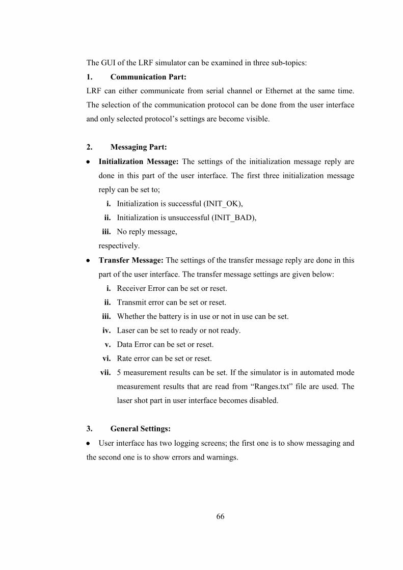
66

The GUI of the LRF simulator can be examined in three sub-topics:

1. Communication Part:

LRF can either communicate from serial channel or Ethernet at the same time.

The selection of the communication protocol can be done from the user interface

and only selected protocol’s settings are become visible.

2. Messaging Part:

•••• Initialization Message: The settings of the initialization message reply are

done in this part of the user interface. The first three initialization message

reply can be set to;

i. Initialization is successful (INIT_OK),

ii. Initialization is unsuccessful (INIT_BAD),

iii. No reply message,

respectively.

•••• Transfer Message: The settings of the transfer message reply are done in this

part of the user interface. The transfer message settings are given below:

i. Receiver Error can be set or reset.

ii. Transmit error can be set or reset.

iii. Whether the battery is in use or not in use can be set.

iv. Laser can be set to ready or not ready.

v. Data Error can be set or reset.

vi. Rate error can be set or reset.

vii. 5 measurement results can be set. If the simulator is in automated mode

measurement results that are read from “Ranges.txt” file are used. The

laser shot part in user interface becomes disabled.

3. General Settings:

•••• User interface has two logging screens; the first one is to show messaging and

the second one is to show errors and warnings.

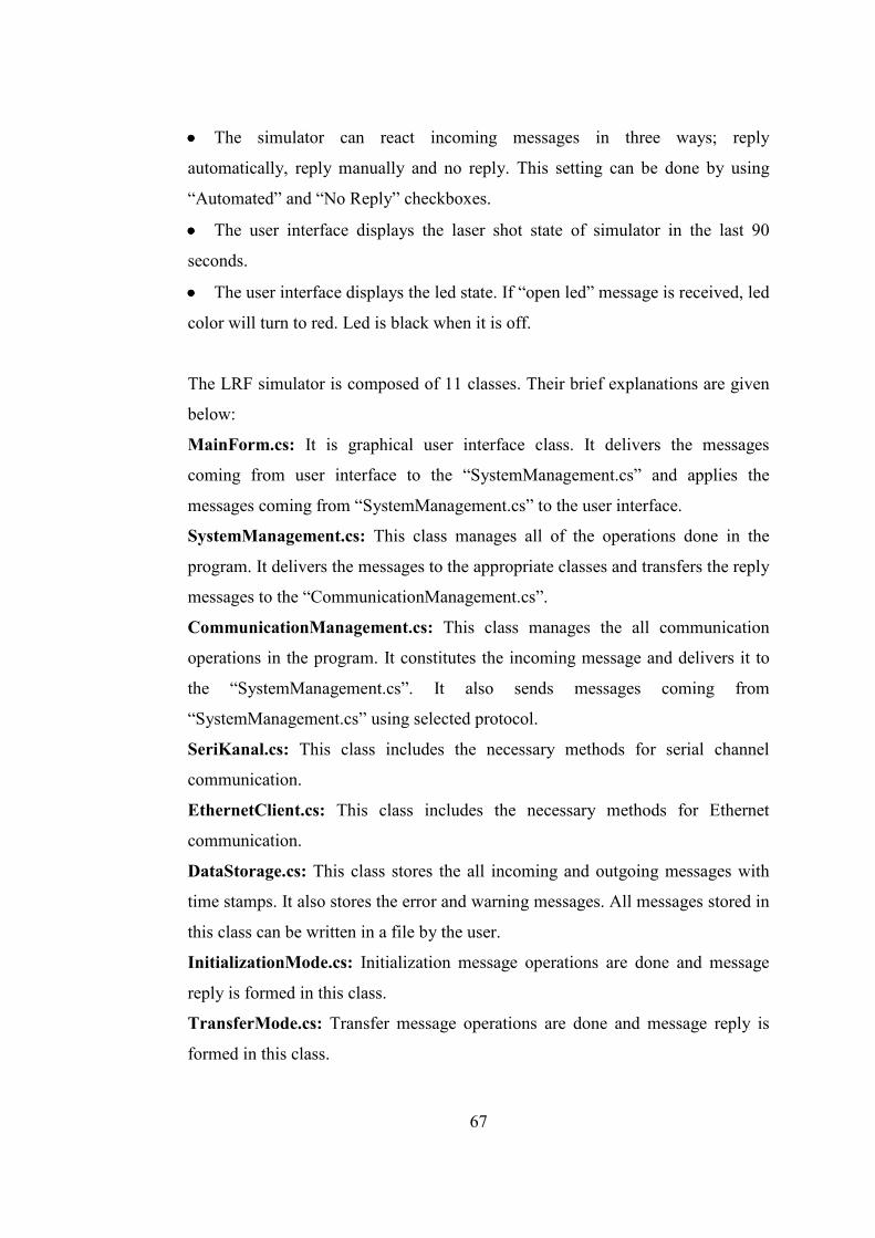
67

•••• The simulator can react incoming messages in three ways; reply

automatically, reply manually and no reply. This setting can be done by using

“Automated” and “No Reply” checkboxes.

•••• The user interface displays the laser shot state of simulator in the last 90

seconds.

•••• The user interface displays the led state. If “open led” message is received, led

color will turn to red. Led is black when it is off.

The LRF simulator is composed of 11 classes. Their brief explanations are given

below:

MainForm.cs: It is graphical user interface class. It delivers the messages

coming from user interface to the “SystemManagement.cs” and applies the

messages coming from “SystemManagement.cs” to the user interface.

SystemManagement.cs: This class manages all of the operations done in the

program. It delivers the messages to the appropriate classes and transfers the reply

messages to the “CommunicationManagement.cs”.

CommunicationManagement.cs: This class manages the all communication

operations in the program. It constitutes the incoming message and delivers it to

the “SystemManagement.cs”. It also sends messages coming from

“SystemManagement.cs” using selected protocol.

SeriKanal.cs: This class includes the necessary methods for serial channel

communication.

EthernetClient.cs: This class includes the necessary methods for Ethernet

communication.

DataStorage.cs: This class stores the all incoming and outgoing messages with

time stamps. It also stores the error and warning messages. All messages stored in

this class can be written in a file by the user.

InitializationMode.cs: Initialization message operations are done and message

reply is formed in this class.

TransferMode.cs: Transfer message operations are done and message reply is

formed in this class.

68

ServiceMode.cs: Service message operations are done and message reply is

formed in this class.

MessageOperations.cs: It is static class. The other classes use the methods of

this class for algorithmic operations.

PulseRateError.cs: This class keeps the history of laser shots done for 90

seconds. It gives the necessary information to the GUI class to display laser shot

state for the past 90 seconds.

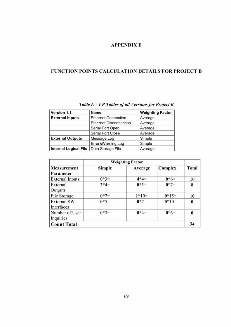
69

APPENDIX E

FUNCTION POINTS CALCULATION DETAILS FOR PROJECT B

Table E – FP Tables of all Versions for Project B

Version 1.1 Name Weighting Factor

External Inputs Ethernet Connection Average Ethernet Disconnection Average Serial Port Open Average Serial Port Close Average External Outputs Message Log Simple Error&Warning Log Simple Internal Logical File Data Storage File Average

Weighting Factor Measurement Parameter

Simple Average Complex Total

External Inputs 0*3= 4*4= 0*6= 16 External Outputs

2*4= 0*5= 0*7= 8

File Storage 0*7= 1*10= 0*15= 10 External SW Interfaces

0*5= 0*7= 0*10= 0

Number of User Inquiries

0*3= 0*4= 0*6= 0

Count Total 34

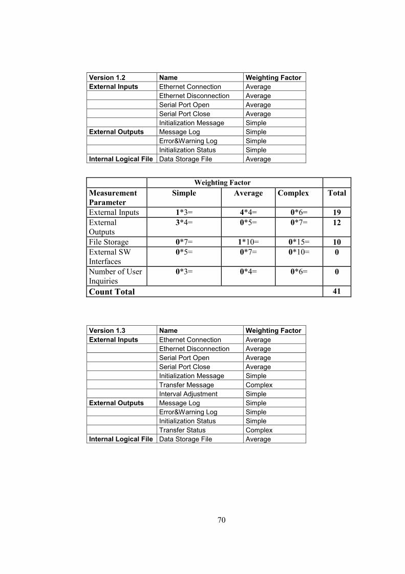
70

Version 1.2 Name Weighting Factor

External Inputs Ethernet Connection Average Ethernet Disconnection Average Serial Port Open Average Serial Port Close Average Initialization Message Simple External Outputs Message Log Simple Error&Warning Log Simple Initialization Status Simple Internal Logical File Data Storage File Average

Weighting Factor Measurement Parameter

Simple Average Complex Total

External Inputs 1*3= 4*4= 0*6= 19 External Outputs

3*4= 0*5= 0*7= 12

File Storage 0*7= 1*10= 0*15= 10 External SW Interfaces

0*5= 0*7= 0*10= 0

Number of User Inquiries

0*3= 0*4= 0*6= 0

Count Total 41

Version 1.3 Name Weighting Factor

External Inputs Ethernet Connection Average Ethernet Disconnection Average Serial Port Open Average Serial Port Close Average Initialization Message Simple Transfer Message Complex Interval Adjustment Simple External Outputs Message Log Simple Error&Warning Log Simple Initialization Status Simple Transfer Status Complex Internal Logical File Data Storage File Average

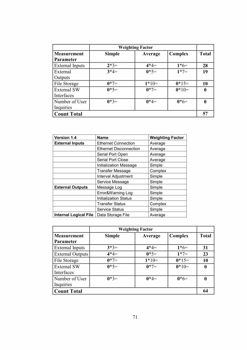
71

Weighting Factor Measurement Parameter

Simple Average Complex Total

External Inputs 2*3= 4*4= 1*6= 28 External Outputs

3*4= 0*5= 1*7= 19

File Storage 0*7= 1*10= 0*15= 10 External SW Interfaces

0*5= 0*7= 0*10= 0

Number of User Inquiries

0*3= 0*4= 0*6= 0

Count Total 57

Version 1.4 Name Weighting Factor

External Inputs Ethernet Connection Average Ethernet Disconnection Average Serial Port Open Average Serial Port Close Average Initialization Message Simple Transfer Message Complex Interval Adjustment Simple Service Message Simple External Outputs Message Log Simple Error&Warning Log Simple Initialization Status Simple Transfer Status Complex Service Status Simple Internal Logical File Data Storage File Average

Weighting Factor Measurement Parameter

Simple Average Complex Total

External Inputs 3*3= 4*4= 1*6= 31 External Outputs 4*4= 0*5= 1*7= 23 File Storage 0*7= 1*10= 0*15= 10 External SW Interfaces

0*5= 0*7= 0*10= 0

Number of User Inquiries

0*3= 0*4= 0*6= 0

Count Total 64

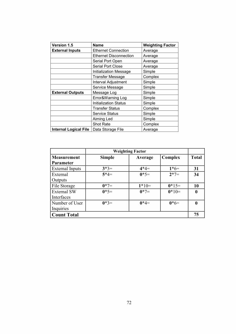
72

Version 1.5 Name Weighting Factor

External Inputs Ethernet Connection Average Ethernet Disconnection Average Serial Port Open Average Serial Port Close Average Initialization Message Simple Transfer Message Complex Interval Adjustment Simple Service Message Simple External Outputs Message Log Simple Error&Warning Log Simple Initialization Status Simple Transfer Status Complex Service Status Simple Aiming Led Simple Shot Rate Complex Internal Logical File Data Storage File Average

Weighting Factor Measurement Parameter

Simple Average Complex Total

External Inputs 3*3= 4*4= 1*6= 31 External Outputs

5*4= 0*5= 2*7= 34

File Storage 0*7= 1*10= 0*15= 10 External SW Interfaces

0*5= 0*7= 0*10= 0

Number of User Inquiries

0*3= 0*4= 0*6= 0

Count Total 75

73

Version 1.6 Name Weighting Factor

External Inputs Ethernet Connection Average Ethernet Disconnection Average Serial Port Open Average Serial Port Close Average Initialization Message Simple Transfer Message Complex Interval Adjustment Simple Service Message Simple Write To File Average External Outputs Message Log Simple Error&Warning Log Simple Initialization Status Simple Transfer Status Complex Service Status Simple Aiming Led Simple Shot Rate Complex Output File Average Internal Logical File Data Storage File Average

Weighting Factor Measurement Parameter

Simple Average Complex Total

External Inputs 3*3= 5*4= 1*6= 35 External Outputs

5*4= 1*5= 2*7= 39

File Storage 0*7= 1*10= 0*15= 10 External SW Interfaces

0*5= 0*7= 0*10= 0

Number of User Inquiries

0*3= 0*4= 0*6= 0

Count Total 84

74

APPENDIX F

OVERALL REPRESENTATION OF PROCESS METRICS

EVALUATED FOR PROJECT A

Table F – Project A Process Metrics

LOC per classes LOC Total

Total Staff Hours

Total # of

Defects FPs

MainGUI.cs : 86 Management.cs : 24 Communication.cs : 28

Version 1.1

EthernetClient.cs : 284

422 17 5 8

MainGUI.cs : 86 Management.cs : 24 Communication.cs : 28 EthernetClient.cs : 284

Version 1.2

SerialChannel.cs : 1298

1720 37 9 16

MainGUI.cs : 449 Management.cs : 29 Communication.cs : 152 EthernetClient.cs : 282

Version 1.3

SerialChannel.cs : 1300

2212 51 12 24

MainGUI.cs : 449 Management.cs : 29 Communication.cs : 152 EthernetClient.cs : 282 SerialChannel.cs : 1300 MessageOperations.cs : 59

Version 1.4

DataStorage.cs : 301

2572 64 15 34

MainGUI.cs : 744 Management.cs : 74 Communication.cs : 152 EthernetClient.cs : 282 SerialChannel.cs : 1300 MessageOperations.cs : 70 DataStorage.cs : 301

Version 1.5

StandByMode.cs : 92

3015 78 18 42

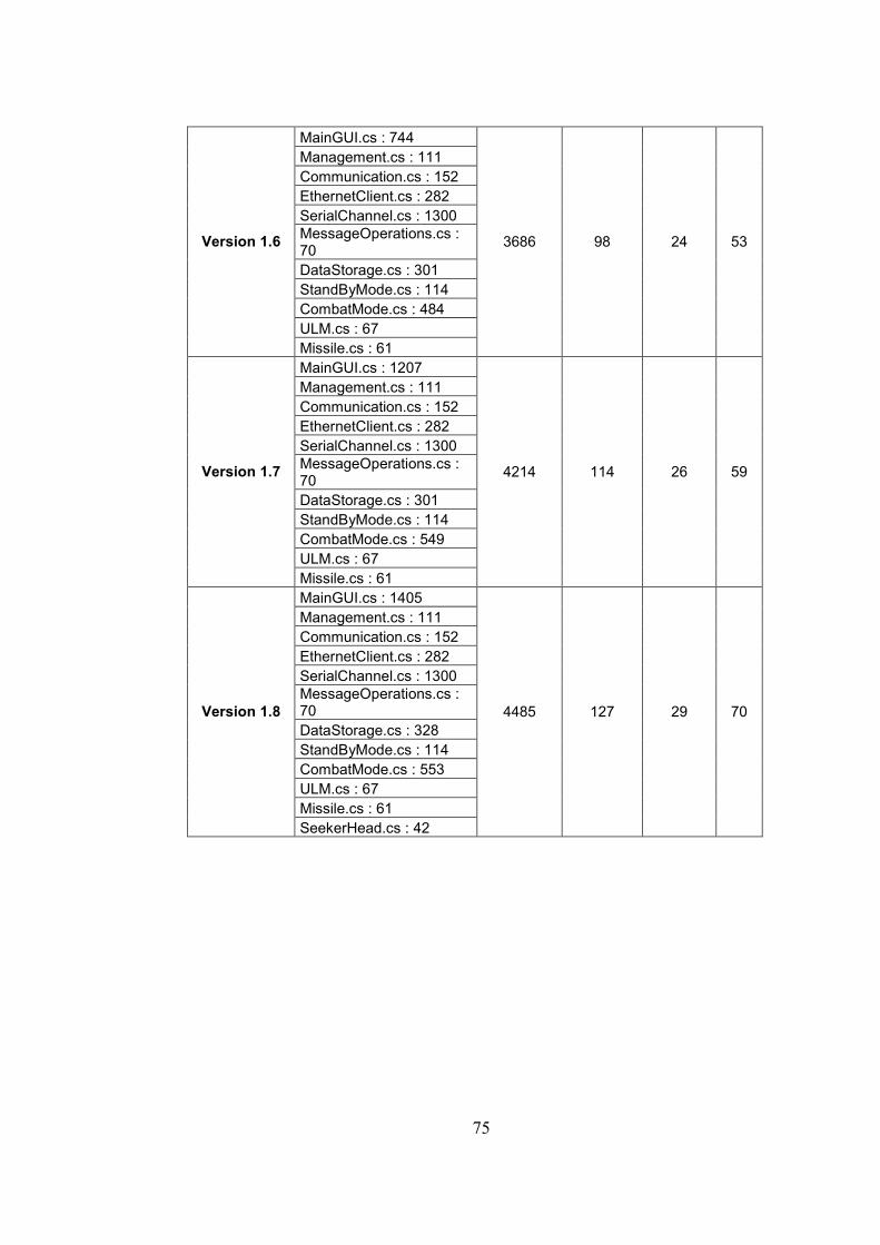
75

MainGUI.cs : 744 Management.cs : 111 Communication.cs : 152 EthernetClient.cs : 282 SerialChannel.cs : 1300 MessageOperations.cs : 70 DataStorage.cs : 301 StandByMode.cs : 114 CombatMode.cs : 484 ULM.cs : 67

Version 1.6

Missile.cs : 61

3686 98 24 53

MainGUI.cs : 1207 Management.cs : 111 Communication.cs : 152 EthernetClient.cs : 282 SerialChannel.cs : 1300 MessageOperations.cs : 70 DataStorage.cs : 301 StandByMode.cs : 114 CombatMode.cs : 549 ULM.cs : 67

Version 1.7

Missile.cs : 61

4214 114 26 59

MainGUI.cs : 1405 Management.cs : 111 Communication.cs : 152 EthernetClient.cs : 282 SerialChannel.cs : 1300 MessageOperations.cs : 70 DataStorage.cs : 328 StandByMode.cs : 114 CombatMode.cs : 553 ULM.cs : 67 Missile.cs : 61

Version 1.8

SeekerHead.cs : 42

4485 127 29 70

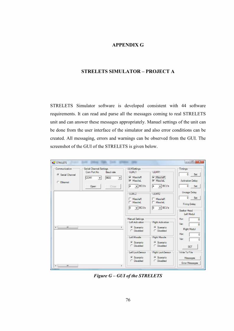
76

APPENDIX G

STRELETS SIMULATOR – PROJECT A

STRELETS Simulator software is developed consistent with 44 software

requirements. It can read and parse all the messages coming to real STRELETS

unit and can answer these messages appropriately. Manuel settings of the unit can

be done from the user interface of the simulator and also error conditions can be

created. All messaging, errors and warnings can be observed from the GUI. The

screenshot of the GUI of the STRELETS is given below.

Figure G – GUI of the STRELETS

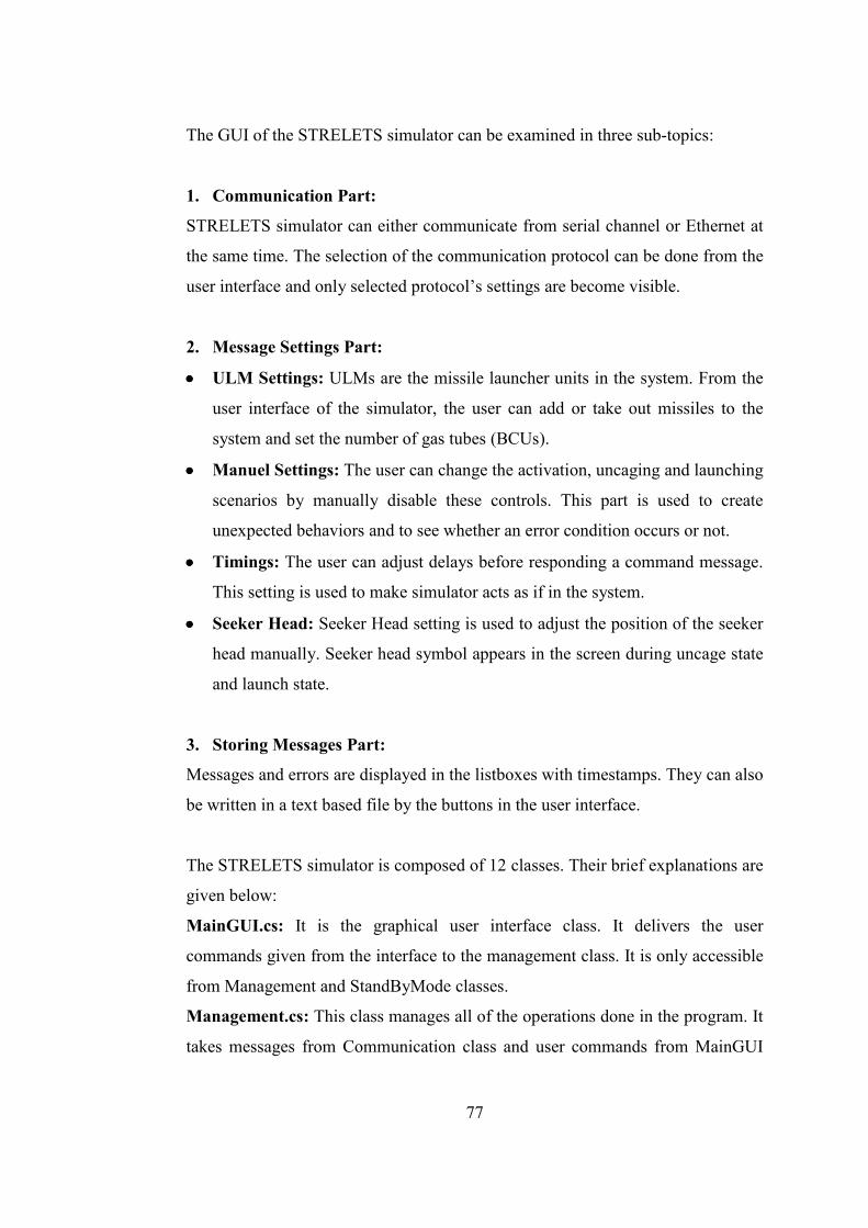
77

The GUI of the STRELETS simulator can be examined in three sub-topics:

1. Communication Part:

STRELETS simulator can either communicate from serial channel or Ethernet at

the same time. The selection of the communication protocol can be done from the

user interface and only selected protocol’s settings are become visible.

2. Message Settings Part:

•••• ULM Settings: ULMs are the missile launcher units in the system. From the

user interface of the simulator, the user can add or take out missiles to the

system and set the number of gas tubes (BCUs).

•••• Manuel Settings: The user can change the activation, uncaging and launching

scenarios by manually disable these controls. This part is used to create

unexpected behaviors and to see whether an error condition occurs or not.

•••• Timings: The user can adjust delays before responding a command message.

This setting is used to make simulator acts as if in the system.

•••• Seeker Head: Seeker Head setting is used to adjust the position of the seeker

head manually. Seeker head symbol appears in the screen during uncage state

and launch state.

3. Storing Messages Part:

Messages and errors are displayed in the listboxes with timestamps. They can also

be written in a text based file by the buttons in the user interface.

The STRELETS simulator is composed of 12 classes. Their brief explanations are

given below:

MainGUI.cs: It is the graphical user interface class. It delivers the user

commands given from the interface to the management class. It is only accessible

from Management and StandByMode classes.

Management.cs: This class manages all of the operations done in the program. It

takes messages from Communication class and user commands from MainGUI

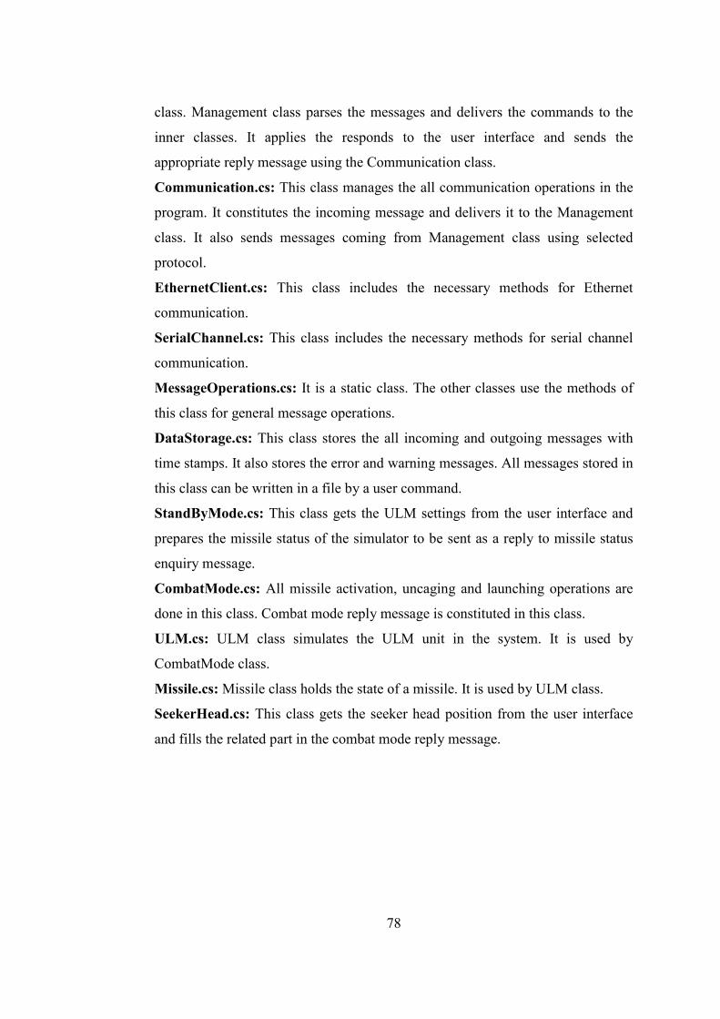
78

class. Management class parses the messages and delivers the commands to the

inner classes. It applies the responds to the user interface and sends the

appropriate reply message using the Communication class.

Communication.cs: This class manages the all communication operations in the

program. It constitutes the incoming message and delivers it to the Management

class. It also sends messages coming from Management class using selected

protocol.

EthernetClient.cs: This class includes the necessary methods for Ethernet

communication.

SerialChannel.cs: This class includes the necessary methods for serial channel

communication.

MessageOperations.cs: It is a static class. The other classes use the methods of

this class for general message operations.

DataStorage.cs: This class stores the all incoming and outgoing messages with

time stamps. It also stores the error and warning messages. All messages stored in

this class can be written in a file by a user command.

StandByMode.cs: This class gets the ULM settings from the user interface and

prepares the missile status of the simulator to be sent as a reply to missile status

enquiry message.

CombatMode.cs: All missile activation, uncaging and launching operations are

done in this class. Combat mode reply message is constituted in this class.

ULM.cs: ULM class simulates the ULM unit in the system. It is used by

CombatMode class.

Missile.cs: Missile class holds the state of a missile. It is used by ULM class.

SeekerHead.cs: This class gets the seeker head position from the user interface

and fills the related part in the combat mode reply message.

79

APPENDIX H

FUNCTION POINTS CALCULATION DETAILS FOR PROJECT A

Table H – FP Tables of all Versions for Project A

Version 1.1 Name Weighting Factor

External Inputs Ethernet Connection Average Ethernet Disconnection Average

Weighting Factor

Measurement Parameter

Simple Average Complex Total

External Inputs 0*3= 2*4= 0*6= 8

External Outputs 0*4= 0*5= 0*7= 0

File Storage 0*7= 0*10= 0*15= 0

External SW Interfaces

0*5= 0*7= 0*10= 0

Number of User Inquiries

0*3= 0*4= 0*6= 0

Count Total 8

Version 1.2 Name Weighting Factor

External Inputs Ethernet Connection Average Ethernet Disconnection Average Serial Port Open Average Serial Port Close Average

80

Weighting Factor

Measurement Parameter

Simple Average Complex Total

External Inputs 0*3= 4*4= 0*6= 16 External Outputs 0*4= 0*5= 0*7= 0 File Storage 0*7= 0*10= 0*15= 0 External SW Interfaces

0*5= 0*7= 0*10= 0

Number of User Inquiries

0*3= 0*4= 0*6= 0

Count Total 16

Version 1.3 Name Weighting Factor

External Inputs Ethernet Connection Average Ethernet Disconnection Average Serial Port Open Average Serial Port Close Average External Outputs Message Log Simple Error&Warning Log Simple

Weighting Factor

Measurement Parameter

Simple Average Complex Total

External Inputs 0*3= 4*4= 0*6= 16 External Outputs 2*4= 0*5= 0*7= 8 File Storage 0*7= 0*10= 0*15= 0 External SW Interfaces

0*5= 0*7= 0*10= 0

Number of User Inquiries

0*3= 0*4= 0*6= 0

Count Total 24

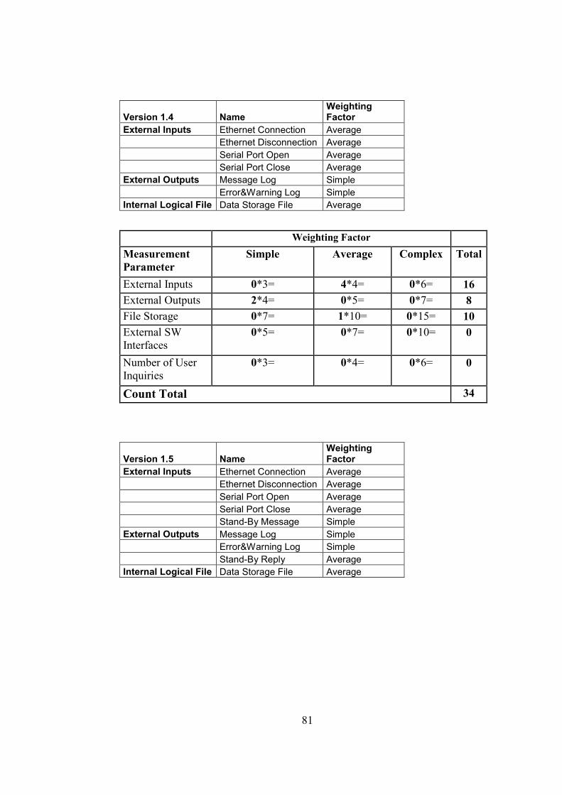
81

Version 1.4 Name Weighting Factor

External Inputs Ethernet Connection Average Ethernet Disconnection Average Serial Port Open Average Serial Port Close Average External Outputs Message Log Simple Error&Warning Log Simple Internal Logical File Data Storage File Average

Weighting Factor

Measurement Parameter

Simple Average Complex Total

External Inputs 0*3= 4*4= 0*6= 16

External Outputs 2*4= 0*5= 0*7= 8

File Storage 0*7= 1*10= 0*15= 10

External SW Interfaces

0*5= 0*7= 0*10= 0

Number of User Inquiries

0*3= 0*4= 0*6= 0

Count Total 34

Version 1.5 Name Weighting Factor

External Inputs Ethernet Connection Average Ethernet Disconnection Average Serial Port Open Average Serial Port Close Average Stand-By Message Simple External Outputs Message Log Simple Error&Warning Log Simple Stand-By Reply Average Internal Logical File Data Storage File Average

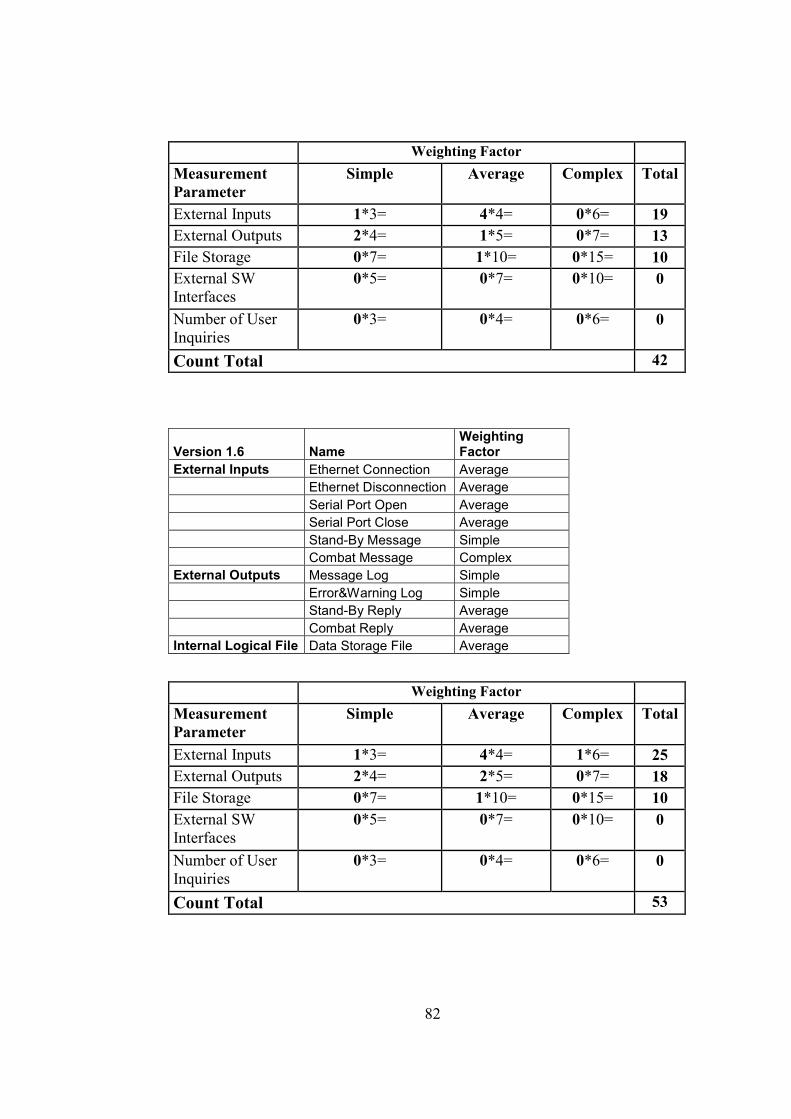
82

Weighting Factor

Measurement Parameter

Simple Average Complex Total

External Inputs 1*3= 4*4= 0*6= 19 External Outputs 2*4= 1*5= 0*7= 13 File Storage 0*7= 1*10= 0*15= 10 External SW Interfaces

0*5= 0*7= 0*10= 0

Number of User Inquiries

0*3= 0*4= 0*6= 0

Count Total 42

Version 1.6 Name Weighting Factor

External Inputs Ethernet Connection Average Ethernet Disconnection Average Serial Port Open Average Serial Port Close Average Stand-By Message Simple Combat Message Complex External Outputs Message Log Simple Error&Warning Log Simple Stand-By Reply Average Combat Reply Average Internal Logical File Data Storage File Average

Weighting Factor

Measurement Parameter

Simple Average Complex Total

External Inputs 1*3= 4*4= 1*6= 25 External Outputs 2*4= 2*5= 0*7= 18 File Storage 0*7= 1*10= 0*15= 10 External SW Interfaces

0*5= 0*7= 0*10= 0

Number of User Inquiries

0*3= 0*4= 0*6= 0

Count Total 53

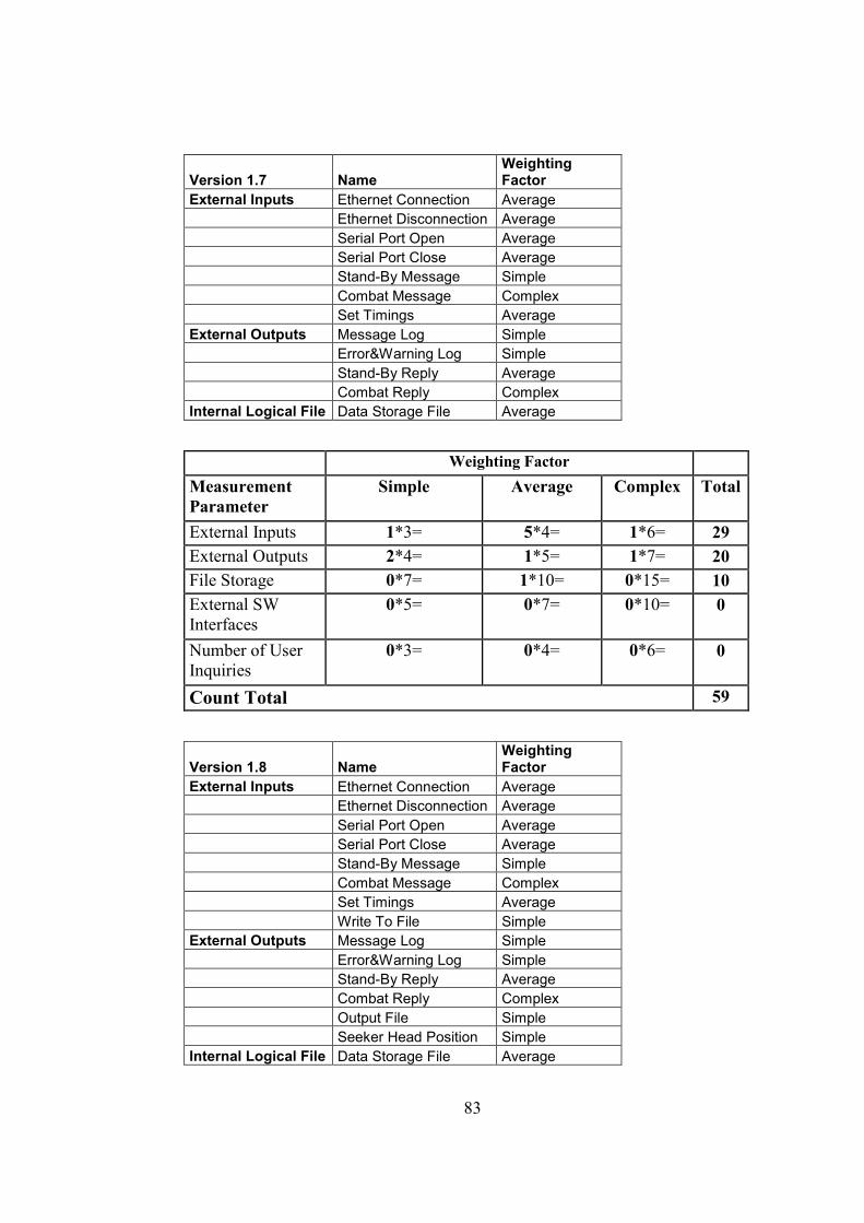
83

Version 1.7 Name Weighting Factor

External Inputs Ethernet Connection Average Ethernet Disconnection Average Serial Port Open Average Serial Port Close Average Stand-By Message Simple Combat Message Complex Set Timings Average External Outputs Message Log Simple Error&Warning Log Simple Stand-By Reply Average Combat Reply Complex Internal Logical File Data Storage File Average

Weighting Factor

Measurement Parameter

Simple Average Complex Total

External Inputs 1*3= 5*4= 1*6= 29 External Outputs 2*4= 1*5= 1*7= 20 File Storage 0*7= 1*10= 0*15= 10

External SW Interfaces

0*5= 0*7= 0*10= 0

Number of User Inquiries

0*3= 0*4= 0*6= 0

Count Total 59

Version 1.8 Name Weighting Factor

External Inputs Ethernet Connection Average Ethernet Disconnection Average Serial Port Open Average Serial Port Close Average Stand-By Message Simple Combat Message Complex Set Timings Average Write To File Simple External Outputs Message Log Simple Error&Warning Log Simple Stand-By Reply Average Combat Reply Complex Output File Simple Seeker Head Position Simple Internal Logical File Data Storage File Average

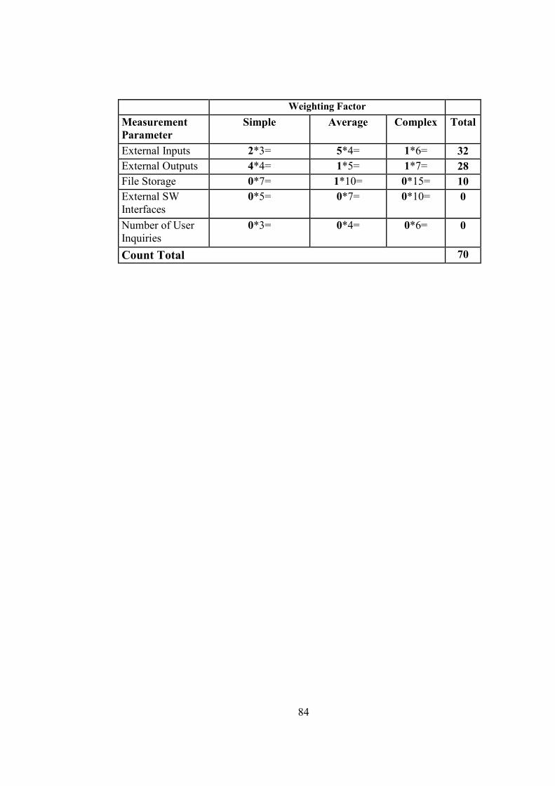
84

Weighting Factor

Measurement Parameter

Simple Average Complex Total

External Inputs 2*3= 5*4= 1*6= 32 External Outputs 4*4= 1*5= 1*7= 28 File Storage 0*7= 1*10= 0*15= 10 External SW Interfaces

0*5= 0*7= 0*10= 0

Number of User Inquiries

0*3= 0*4= 0*6= 0

Count Total 70