the effects of the saving and banking glut on the u.s. …gep575/sbg5.pdf · fed governor ben...

THE EFFECTS OF THE SAVING AND BANKING GLUTON THE U.S. ECONOMY

ALEJANDRO JUSTINIANO, GIORGIO E. PRIMICERI, AND ANDREA TAMBALOTTI

Abstract. We use a quantitative equilibrium model with houses, collateralized debt and

foreign borrowing to study the impact of global imbalances on the U.S. economy in the

2000s. Our results suggest that the dynamics of foreign capital flows account for between

one fourth and one third of the increase in U.S. house prices and household debt that

preceded the financial crisis. The key to these findings is that the model generates the

sustained low level of interest rates observed over that period.

1. Introduction

Before the financial crisis of 2007-08, most observers saw the growing international im-

balances in the trade of goods and assets as the main source of vulnerability for the U.S.

and the world economy (e.g. Roubini and Setser, 2005, Obstfeld and Rogoff, 2007, Krug-

man, 2007). As shown in figure 1.1, the U.S. trade deficit had been growing since the

mid 1990s, reaching 6 percent of GDP at its peak in 2006, mostly financed by emerging

Asia (especially China) and the oil-exporting countries. In a very influential speech, then

Fed Governor Ben Bernanke (2005) attributed these imbalances to a “Global Saving Glut”

(SG), which he described as an excess of saving in developing countries primarily directed

towards riskless assets in the United States. Given these lopsided patterns of international

exchange, many feared that a sudden loss of appetite for U.S. assets by international in-

vestors might precipitate an abrupt adjustment of its current account deficit, with serious

repercussions for the world economy.

Although a catastrophic financial crisis did eventually occur, its epicenter was the Amer-

ican housing market, rather than the international market for assets and goods. As a conse-

quence, most of the early literature on the causes and consequences of the crisis focused on

Date: August 2013. First Draft: June 2013.We would like to thank our discussants Klaus Adam, Federico Signoretti, and Martin Uribe for their usefulsuggestions, and Efrem Castelnuovo, Gianluca Benigno, Andrea Ferrero, Andrea Raffo and participants inseveral conferences and seminars for comments. Aaron Kirkman and Todd Messer provided outstandingresearch assistance. The views expressed in this paper are those of the authors and are not necessarilyreflective of views at the Federal Reserve Banks of Chicago, New York or the Federal Reserve System.

1

THE EFFECTS OF THE SAVING AND BANKING GLUT ON THE U.S. ECONOMY 2

1990 1992 1994 1996 1998 2000 2002 2004 2006 2008 2010 2012

40

60

80

100

120

140

160

180

7

6

5

4

3

2

1

0

HousePrices

Trad

eBa

lanceto

GDPRa

tio

Trade Balance to GDP RatioFHFA (2000:Q1=100)CoreLogic (2000:Q1=100)

Figure 1.1. U.S. trade balance-to-GDP ratio (left axis) and real houseprices (right axis). The two measures of house prices are the FHFA (formerlyOFHEO) all transactions house price index and the CoreLogic repeated-salesindex.

the features of U.S. financial markets—regulation, risk-management, securitization, fund-

ing models—that contributed to the credit and housing boom of the first half of the 2000s,

whose reversal was the proximate cause of the crisis.1

A more recent strand of literature, however, has brought back into focus the connection

between the global imbalances that preceded the crisis and the credit and housing boom

that precipitated it.2 On the empirical side, this literature points to the depressing effect

of capital inflows on U.S. interest rates and spreads, whose low levels contributed to the

boom in mortgage debt and house prices before the crisis (Bernanke et al., 2011, Bertaut

et al., 2011, Warnock and Warnock, 2009). Bertaut et al. (2011), for instance, estimate

that the purchases of Treasury and Agency debt by the SG countries over the period 2003

to 2007, amounting to roughly one trillion dollars, lowered long-term interest rates in the

U.S. by between 110 and 140 basis points.

1See Brunnermeir (2009) for an early overview. Demyanyk and van Hemert (2011), Ashcraft and Schuer-mann (2008), Adrian and Shin (2010), Pozsar et al. (2010), Gorton (2009), and Mian and Sufi (2009),among many others, provide more detailed accounts of the events of the crisis and of some of the importantmechanisms at play, with a special focus on subprime mortgages and their securitization. In fact, in thisearly phase, this sequence of events was most often described as the “subprime crisis.”2Obstfeld and Rogoff (2009) is one of the first papers forcefully arguing that global imbalances and thefinancial crisis are intimately related.


Moreover, careful detective work by Bertaut et al. (2011) in tracking the flows of capital

to and from the United States has uncovered another channel through which international

capital flows might have contributed to easier financial conditions in the U.S. before the

crisis. Indeed these authors document that after 2003, European banks played an increasing

role in the market for safe U.S. assets, especially the AAA tranches of private label asset-

backed securities (ABS) that turned out to be far from riskless in the crisis. Since Europe’s

current account vis-a-vis the U.S. was roughly balanced, these gross positions of European

banks in ABS were funded by direct borrowing in the dollar wholesale credit market. As

a result, these financial institutions became an integral part of the financial intermediation

sector in the U.S., in direct competition with domestic financial institutions, as also pointed

out by Acharya and Schnabl (2009).

Shin (2012) refers to these gross flows from international banks into mortgage products,

even in the absence of corresponding net imbalances, as the “Global Banking Glut” (BG),

in juxtaposition to the Global Saving Glut associated with the U.S. current account deficit.

According to his analysis, the flow of funds associated with the BG played an important

role in easing financial conditions in the United States during the boom, comparable in

magnitude to that of the purchases of Government debt by the SG countries.

In Shin’s (2012) model of global banking, spreads are negatively related to the total

amount of funds intermediated by the financial system . When risk recedes, banks expand

their balance sheet and spreads fall. This motivates Shin’s claim that higher total inter-

mediation generated by European banks lowered the spreads between safe funding rates

and the returns on ABS, and therefore ultimately on mortgages. Consistent with this view,

Bertaut at al. (2011) estimate that the increase in the demand for ABS and similar instru-

ments by European banks over the period 2003-2007 contributed to a decline in their yield

of between 60 and 160 basis points, depending on the instruments and the methodology.3

When the boom turned to bust, and the market for private-label ABS in which European

banks were most active disappeared, the mechanism worked in reverse, contributing to the

propagation of the U.S. financial crises around the world (Obstfeld, 2012, Acharya and

Schnabl, 2009).

3These estimates represent an upper bound on the effect of the BG on U.S. rates, since they do not accountfor the endogenous response in the supply of ABS and similar assets. The production of these assets rosedramatically during this period, in part to satisfy the increase in demand by U.S. and foreign investors.


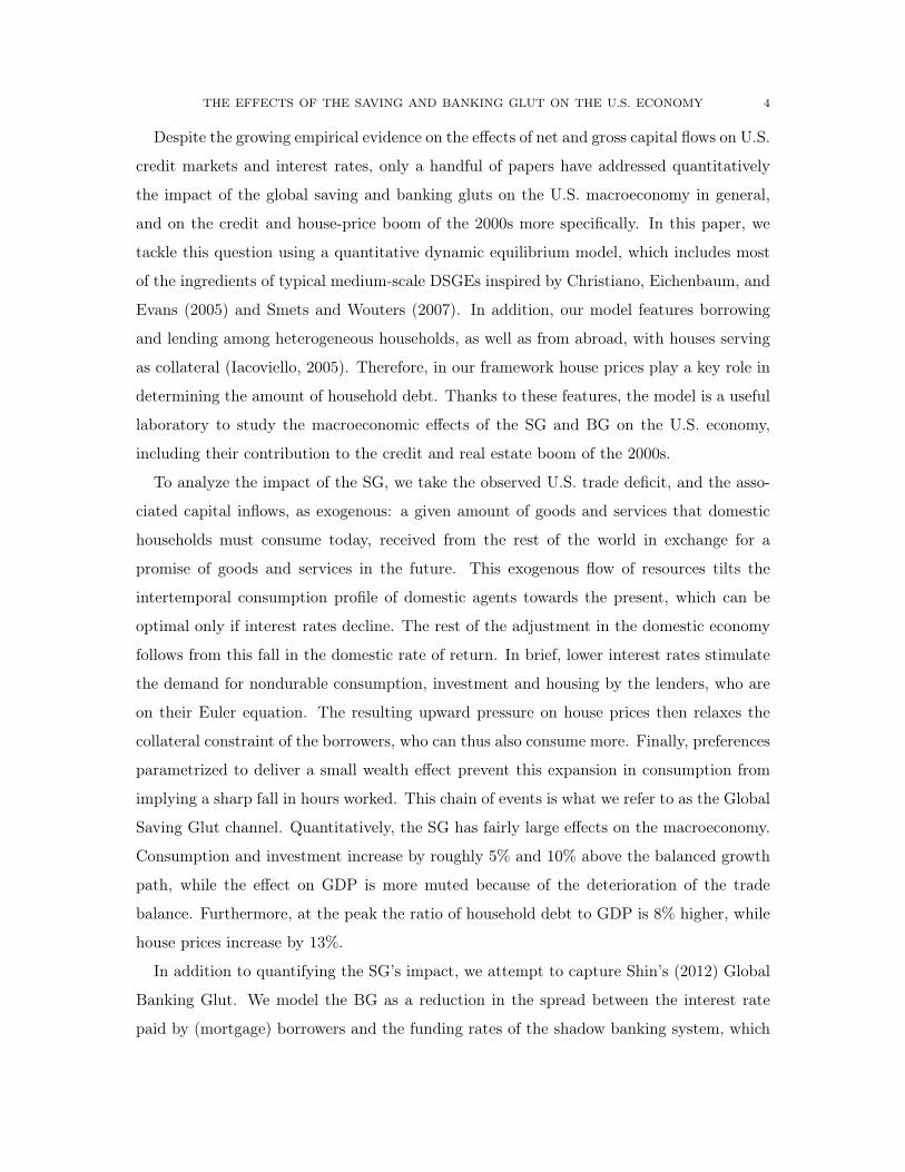
Despite the growing empirical evidence on the effects of net and gross capital flows on U.S.

credit markets and interest rates, only a handful of papers have addressed quantitatively

the impact of the global saving and banking gluts on the U.S. macroeconomy in general,

and on the credit and house-price boom of the 2000s more specifically. In this paper, we

tackle this question using a quantitative dynamic equilibrium model, which includes most

of the ingredients of typical medium-scale DSGEs inspired by Christiano, Eichenbaum, and

Evans (2005) and Smets and Wouters (2007). In addition, our model features borrowing

and lending among heterogeneous households, as well as from abroad, with houses serving

as collateral (Iacoviello, 2005). Therefore, in our framework house prices play a key role in

determining the amount of household debt. Thanks to these features, the model is a useful

laboratory to study the macroeconomic effects of the SG and BG on the U.S. economy,

including their contribution to the credit and real estate boom of the 2000s.

To analyze the impact of the SG, we take the observed U.S. trade deficit, and the asso-

ciated capital inflows, as exogenous: a given amount of goods and services that domestic

households must consume today, received from the rest of the world in exchange for a

promise of goods and services in the future. This exogenous flow of resources tilts the

intertemporal consumption profile of domestic agents towards the present, which can be

optimal only if interest rates decline. The rest of the adjustment in the domestic economy

follows from this fall in the domestic rate of return. In brief, lower interest rates stimulate

the demand for nondurable consumption, investment and housing by the lenders, who are

on their Euler equation. The resulting upward pressure on house prices then relaxes the

collateral constraint of the borrowers, who can thus also consume more. Finally, preferences

parametrized to deliver a small wealth effect prevent this expansion in consumption from

implying a sharp fall in hours worked. This chain of events is what we refer to as the Global

Saving Glut channel. Quantitatively, the SG has fairly large effects on the macroeconomy.

Consumption and investment increase by roughly 5% and 10% above the balanced growth

path, while the effect on GDP is more muted because of the deterioration of the trade

balance. Furthermore, at the peak the ratio of household debt to GDP is 8% higher, while

house prices increase by 13%.

In addition to quantifying the SG’s impact, we attempt to capture Shin’s (2012) Global

Banking Glut. We model the BG as a reduction in the spread between the interest rate

paid by (mortgage) borrowers and the funding rates of the shadow banking system, which


are tied in turn to the interest rate earned by savers. In our model, this spread between

borrowing and lending rates reflects the market power of financial intermediaries, which

channel funds to the impatient households from both the domestic patient ones and the

rest of the world. More competition in this market therefore implies lower spreads. This

is the channel through which the entry of European players in the intermediation market,

which is at the heart of the Global Banking Glut hypothesis, affects credit conditions in

the model.

This simple modeling approach captures the first order effect on macroeconomic outcomes

of the entry of European banks in the American intermediation market. A reduction in

spreads is also an outcome of the more sophisticated and realistic model of intermediation

proposed by Shin (2012) to formalize the effects of the Global Banking Glut. Of course,

that model has many more implications than ours regarding the behavior of intermediaries,

but it is silent on their macroeconomic consequences.

In our simulations, the reduction in spreads due to the BG reduces the interest rate and

makes houses more valuable for the borrowers, relative to nondurable goods. This shift in

demand towards houses increases their price and relaxes the collateral constraint, allowing

the borrowers to obtain more credit. In this case without capital inflows, the increase in

credit is financed by additional lending from the domestic savers. Hence, the response

of savers to the BG tends to be opposite to that of the borrowers, leading to fairly muted

effects on aggregate variables. This is in contrast with the SG case, where the fall in interest

rates stimulates demand by both types of households. Overall, our experiments attribute

to the combined effect of the BG and SG between one fourth and one third of the increase

in house prices and household debt during the years leading up to the financial crisis.

1.1. Related literature. Among the first papers to formally address the saving glut hy-

pothesis were Caballero, Farhi, and Gourinchas (2008), and Mendoza, Quadrini, and Rios-

Rull (2009). These influential contributions share a focus on the differences in financial

market development across countries that made riskless U.S. assets a particularly appeal-

ing store of value for the excess saving in the rest of the world. In their detailed quantitative

exercise, Mendoza, Quadrini, and Rios-Rull (2009) also trace the dynamic implications of

global financial liberalization on international imbalances and portfolios. However, they

concentrate much less then we do on the broader macroeconomic implications in the United

States.


Our work is more closely related to a recent literature connecting current account deficits

and foreign capital flows into the U.S. to the housing and credit booms that preceded the

financial crisis. This literature is far from unanimous on the importance of this international

channel for macroeconomic developments in the United States. At one extreme of this

spectrum, Favilukis et al. (2012 and 2013) find virtually no effect of the foreign purchases

of Government bonds on house prices and domestic credit. In their rich model, the reduction

in the risk-free rate associated with the flow of international resources into the U.S. economy

is offset by an increase in the risk premium on housing, due to the portfolio reallocation

forced on domestic agents by the foreign purchases of safe assets.4 In our model, on the

contrary, there is no risk, and hence no meaningful portfolio choice, since agents have

perfect foresight. As a consequence, our results highlight the intertemporal substitution

mechanisms associated with the fall in interest rates triggered by the trade deficit. On

the one hand, this stricter macroeconomic focus comes at the cost of ignoring a potentially

important portfolio channel and might bias our quantitative conclusions. On the other hand,

the irrelevance of portfolio choice in our model allows us to take a more comprehensive view

of the saving glut, without having to worry about the composition of the capital inflows.

Moreover, it enables us to calibrate the foreign impulse to the total trade deficit, rather

than just to the fraction corresponding to the purchases of Treasuries, as Favilukis et al.

(2012) do.

Our results are more in line with those of Adam, Kuang, and Marcet (2011), Garriga,

Manuelli, and Peralta-Alva (2012), and Kiyotaki, Michaelides, and Nikolov (2011), who all

find large effects of a decline in the world interest rate on house prices in small open economy

models calibrated on the U.S. experience of the 2000s, despite important differences in their

modeling approaches. In Adam et al. (2011), the large reaction of house prices is due to

the presence of agents with subjective beliefs about these prices. In Garriga et al. (2012),

the quantitative results hinge on combining lower real interest rates and looser financial

conditions, while we abstract from the latter. Furthermore, unlike these papers, we model

the domestic country as large, and populated by both borrowers and savers, which makes

interest rates endogenous and creates interesting dynamics from the interplay of the two

classes of agents. In this respect, we are closer to Kiyotaki et al. (2011), who focus on

4Caballero and Krishnamurty (2009) also highlight the increase in risk borne by domestic agents followingthe absorption of safe assets by foreigners.


the redistributive effects of changes in the world interest rate across net buyers and net

sellers of houses. Finally, Ferrero (2012) also addresses the correlation between current

account deficits and house prices within a two-country model, but with one representative

international saver lending to one representative borrower in the U.S.

The analysis of the BG is a distinctive feature of our paper, relative to these other

contributions. In this respect, we also make contact with the small-open economy business

cycle literature that has emphasized the role of risk premia and spreads as an important

source of business cycle fluctuations (e.g. Neumeyer and Perri 2005, Garcıa-Cicco, Pancrazi,

and Uribe, 2010).

The rest of the paper proceeds as follows. Section 2 describes the model, whose calibration

is presented in section 3. Section 4 presents the model’s dynamics in response to three

impulses: an increase in the trade deficit that captures the saving glut; a fall in the spread

between borrowing and lending rates, which captures the banking glut; and a combination

of the two. Section 5 concludes.

2. Model

This section presents the quantitative general equilibrium model we use to analyze the

impact of the SG and BG on the U.S. economy, including their effect on the recent boom in

the debt of U.S. households and in real estate prices. The model builds on Iacoviello (2005)

and Campbell and Hercowitz (2009). The key assumption is that domestic households

have heterogeneous desires to save, which generate borrowing and lending among them, as

well as from abroad. Debt, which we often call “mortgages”, is collateralized by houses, to

capture the fact that mortgages represent by far the most important component of U.S.

households’ liabilities.

The economy is populated by four main classes of domestic agents—households, house

producers, goods producers and a government. Households can borrow from each other

through a financial intermediation sector composed of monopolistic investment banks and

competitive commercial banks, which also collect funds from abroad.

2.1. Households. There are two types of households, which differ by the rate at which

they discount the future. Patient households are denoted by l, since in equilibrium they

are the ones saving and lending. They represent a share 1 − ψ of the population, and we


interchangeably refer to them as the lenders or savers. Their discount factor is βl > βb,

where βb is the discount factor of the impatient borrowers. At time 0, representative

household j = b, l maximizes the utility function

E0

∞�

t=0

βtj

�C

�j,tH

1−�j,t − ϕXj,tL

1+ηj,t

�1−σ− 1

1− σ,

where

Xj,t =�C

�j,tH

1−�j,t

�µX

1−µj,t−1.

In these expressions, Cj,t denotes consumption of nondurable goods, Hj,t is the stock of

houses, and Lj,t is hours worked. This specification of the utility function is similar to the

one proposed by Jaimovich and Rebelo (2009). When µ = 1, it belongs to the class of

utility functions recommended by King, Plosser, and Rebelo (1988). When µ = 0, these

preferences resemble those of Greenwood, Hercowitz, and Huffman (1988), with no wealth

effect on labor supply. The difference from Jaimovich and Rebelo (2009) is that households

in this model derive utility from a Cobb-Douglas aggregator of non-durable consumption

goods and housing services (assumed to be proportional to the stock of housing). The

parameter � denotes the share of nondurable consumption in this composite good.

The utility maximization problem is subject to the nominal flow budget constraint

PtCj,t + Pht Ξj,t + PtIj,t +Rj,t−1Dj,t−1 ≤ Wj,tLj,t +R

ktKj,t +Πj,t − PtTj,t +Dj,t.

In this expression, Pt and Pht are the prices of the consumption good and of houses, while

Rkt and Wj,t are the nominal rental rates of capital and labor. The wage is indexed by j

because the labor input of the borrowers is not a perfect substitute for that of the savers.

Dj,t is the amount of one period nominal debt (or deposits, when negative) accumulated

by the end of period t, and carried into period t+ 1, with gross nominal interest rate Rj,t.

The interest rate depends on j because the return paid by borrowers and that earned by

lenders differ due to the presence of a spread in the financial intermediation sector. Πj,t

is the share of profits of the intermediate firms and of investment banks accruing to each

household of type j, and Tj,t are lump-sum taxes and transfers from the government.

The stocks of houses and capital evolve according to the accumulation equations

Hj,t+1 = (1− δh)Hj,t + Ξj,t


(2.1) Kj,t+1 = (1− δk)Kj,t +

�1− Sk

�Ij,t

Ij,t−1

��Ij,t,

where Ξj,t represents new houses, Ij,t is investment in productive capital, and δh and δk

are the rates of depreciation of the two stocks. The function Sk captures the presence of

adjustment costs in investment, as in Christiano, Eichenbaum, and Evans (2005), and is

parametrized as follows

(2.2) Sk (x) = ζk1

2(x− e

γ)2 ,

so that, in steady state, Sk = S�k = 0 and S

��k = ζk > 0, where e

γ is the economy’s growth

rate along the balanced growth path, further described below. Finally, we assume that

the total supply of new houses (Ξt) grows at the constant rate of technological progress,

which corresponds to imposing infinite costs for adjusting the production of new houses. In

section 4.3, we also consider a more complex specification in which new houses are produced

combining land and residential investment.

2.1.1. The borrowing limit. Households’ ability to borrow is limited by a collateral con-

straint, similar to Kiyotaki and Moore (1997). We model this constraint to mimic the asym-

metry of mortgage contracts, as in Justiniano, Primiceri, and Tambalotti (2012). When

real estate prices increase, households can refinance their loans and therefore borrow more

against the higher value of the entire housing stock. When prices fall, however, the lower

collateral value leads to less lending against new houses, but lenders cannot require faster

repayment of the debt already outstanding.

More formally, we write the collateral constraint as

Dj,t ≤ D̄j,t =

θPht Hj,t+1 if P h

t ≥ Pht−1

(1− δh) D̄j,t−1 + θPht Ξj,t if P h

t < Pht−1.

If collateral values increase (i.e. Pht rises), households can borrow up to a fraction θ of

the current value of their entire housing stock. This is the standard formulation of the

collateral constraint, which implicitly assumes that all outstanding mortgages will be refi-

nanced to take advantage of the new, more favorable conditions. On the contrary, if P ht

falls, households need not repay the outstanding balance on their mortgage, over and above


the repayment associated with the depreciation of the housing stock (δh).5 Therefore, the

new less favorable credit conditions only apply to the flow of new mortgages, collateralized

by the most recent house purchases.

This asymmetry of the borrowing limit makes debt in the model very similar to an

adjustable-rate mortgage, in which the interest rate changes every quarter, but the principal

can only be adjusted by the borrower, either through a cash-out refinancing, or through

pre-payment. Therefore, this modeling device captures an important feature of long-term

mortgages over real estate cycles, namely the downward stickiness of the principal. During

booms, homeowners take advantage of rising property values through refinancing, which

reduces the effective duration of outstanding mortgages. During busts, on the contrary,

existing homeowners cannot be forced to pay down their outstanding debt (over and above

the contractual amortization), even if the value of the collateral falls.

Given their low desire to save, impatient households borrow from the patient in equi-

librium. In fact, local to the steady state, they borrow up to the collateral constraint.

Therefore, they choose not to hold any capital: absent the constraint, they would borrow

even more, so it is clearly not optimal for them to hold any asset other than houses. For

simplicity, we impose that borrowers do not accumulate capital also when the collateral con-

straint does not bind away from the steady state, even if it might occasionally be optimal

for them to do so.

2.2. Goods producers. There is a continuum of intermediate firms indexed by i ∈ [0, 1],

each producing a good Yt (i), and a competitive final good sector producing output Yt

according to

Yt =

�ˆ 1

0Yt(i)

11+λdi

�1+λ

.

Intermediate firms, which are owned by the lenders, operate the constant-return-to scale

production function

(2.3) Yt (i) = A1−αt K

αt (i)

�(ψLb,t (i))

ν ((1− ψ)Ll,t (i))1−ν

�1−α−AtF .

5This formulation assumes that the amortization rate of the mortgage coincides with the depreciation rateof the housing stock. In Justiniano, Primiceri, and Tambalotti (2012) we also experiment with higheramortization rates, so that households build equity in their house over time, as in Campbell and Hercowitz(2009).


They rent labor (of the two types) and capital on competitive markets paying Wb,t, Wl,t

and Rkt respectively. F represents a fixed cost of production, and is chosen to ensure that

steady state profits are zero. The labor augmenting technology factor At grows at rate γ.

The intermediate firms operate in monopolistically competitive markets and set their

price Pt (i) subject to a nominal friction as in Calvo (1983). A random set of firms of

measure 1 − ξp optimally reset their price every period, subject to the demand for their

product, while the remaining ξp fraction of prices do not change. In section 4.1, we describe

how the presence of sticky prices amplifies the expansionary effect of the SG on labor

demand and the equilibrium level of production.

2.3. Fiscal and monetary policy. The government collects taxes, pays transfers, con-

sumes a fraction of final output, and sets the nominal interest rate.

We assume that government spending is a constant fraction g of final output, and that

the government balances it’s budget, i.e.

Gt = gYt = ψTb,t + (1− ψ)Tl,t.

In addition, we assume that total taxes levied on borrowers represent a constant share χ of

the financing needs of the government, i.e.

ψTb,t = χGt.

If χ = 0, the entire tax burden is on the savers, while if χ = ψ borrowers and savers pay

the same amount per-capita. Therefore, we can interpret the parameter χ as capturing the

extent of government redistribution. Given the presence of borrowing-constrained agents

and the redistributive nature of the tax rule, Ricardian equivalence does not hold in our

model. Therefore, the balanced budget assumption is not entirely innocuous, but just a

simplification that allows us to abstract from the details of how the government finances

its expenditures, as is the assumption of lump-sum taxes.

Monetary policy sets the short-term nominal interest rate on deposits based on the

feedback rule

Rl,t

Rl= max

1

Rl;

�Rl,t−1

Rl

�ρR��

(πt · πt−1 · πt−2 · πt−3)1/4

π

�τπ �Yt

Y∗t

�τy�1−ρR

,


where πt is the gross rate of inflation, π is the Central Bank’s inflation target, and Y∗t is

the trend level of output that grows at the constant rate of technological progress. The

parameters ρR, τπ and τy capture the degree of inertia, and the strength of the interest rate

reaction to the deviations of annual inflation from the target and of output from trend.

2.4. Financial intermediaries. The financial intermediation sector transfers resources to

the borrowers from savers at home and in the rest of the world. The sector consists of in-

vestment banks, which do the lending, and retail banks, which collect deposits. Investment

banks fund the purchase of mortgages by issuing securities, say asset-backed commercial

paper, on a non-competitive wholesale credit market. Retail banks (or money market mu-

tual funds) buy these securities using the deposits that they collect. In the process, the

investment banks earn a profit in the form of a spread between the mortgage rate and their

funding rate, which is equal to the retail deposit rate paid to savers.

We assume that this spread derives from market power exercised by investment banks

in the wholesale funding market, for instance by creating differentiated credit products

that they sell to commercial banks and money market mutual funds. The existence of

this market power can be microfounded through a monopolistic competition structure as

in Gerali at al.’s (2010) DSGE model of banking. Alternatively, we could assume that the

spread earned by investment banks derives from the costs of intermediation that each of

them sustains, as in Curdia and Woodford (2009) for instance.

In either case, what is relevant for our analysis is only that the spread falls when Euro-

pean banks enter the wholesale credit market, as suggested by Shin’s (2012) global banking

glut hypothesis. Under monopolistic competition, this compression in the markup follows

naturally when new competitors enter the market. With intermediation costs, instead,

spreads fall if entry reduces each bank’s market footprint, and hence its volume of interme-

diation, under the conventional assumption that the cost is convex in the amount of funds

intermediated.6

6For our purposes, this intermediation structure is equivalent to one with a third layer of intermediation,in which individual mortgages are securitized and sold to investment banks and other participants in theshadow banking system, rather than purchased directly by them. This more complex structure wouldbe equivalent to the one presented here because the margin that is relevant for the global banking gluthypothesis that we are trying to capture is the one between wholesale funding and mortgage products,rather than the one between mortgages and mortgage-backed securities.


2.4.1. Investment banks. Investment banks purchase mortgages with funds they raise in the

wholesale credit market, by issuing a continuum of differentiated credit instruments indexed

by n ∈ [0, Nt] . Each of these instruments carries a net interest rate rt (n), while mortgages

accrue net interest of rb,t. Therefore, the profit earned from funding Db,t (n) dollars worth

of mortgages by selling Lt (n) dollars of instrument n is

Πt (n) = rb,tDb,t (n)− rt (n)Lt (n) ,

where one dollar in wholesale funding turns into one dollar in mortgages, so that Db,t (n) =

Lt (n) .

2.4.2. Retail banks. Retail banks collect a total amount of deposits

Dt = − (1− ψ)Dl,t +Df,t,

where − (1− ψ)Dl,t come from the lenders and Df,t come from the RoW.7 The net interest

rate paid on these deposits is rl,t, and they are invested in the securities issued by investment

banks, generating total profits for the retail banking sector in the amountˆ Nt

0rt (n)Lt (n) dn− rl,tDt.

We assume that retail banks have a taste for a diversified portfolio, which implies a

downward sloping demand function for each instrument issued by the investment banks,

with elasticity ε (Nt). For instance, under the translog specification proposed by Feenstra

(2003), this elasticity would be ε (Nt) = − (1 + εNt) (e.g. Bilbiie, Ghironi, and Melitz,

2012). As the number of instruments available on the market increases, they become closer

substitutes, and the elasticity of demand increases.

2.4.3. Equilibrium, spread and market clearing. The taste for portfolio diversification of

retail banks generates monopoly power in the wholesale credit market, which investment

banks exploit by selling their securities at a discount with respect to the interest rate

charged to borrowers. As a result, in the symmetric equilibrium in which all securities pay

the same interest rate, we have

rb,t = µ (Nt) rl,t,(2.4)

7Recall that Dl,t denotes debt if positive and deposits if negative. Similarly, a positive Df,tcorresponds toforeign holdings of U.S. debt.


where the spread in the borrowing over the lending rate µ (Nt) depends on the size of

the market Nt. Under the translog specification, this function is µt (Nt) = 1 + (εNt)−1.

Alternatively, if the portfolio purchased by retail banks were a CES aggregate of a discrete

set of Nt instruments, we would obtain µt (Nt) = [ε (Nt − 1) +Nt] / [ε (Nt − 1)], as in

Jaimovich and Floetotto (2008). Intuitively, both of these parametrizations imply that

markups fall as the number of competitors increases. However, in our calibration we do

not exploit any specific mapping between Nt and µt, and instead we calibrate directly the

decline in spreads due to the entry of European players.

In the symmetric equilibrium, in which one dollar of deposits turns into one dollar of

wholesale lending and one dollar of loans, with no deadweight loss from interest rate dis-

persion, market clearing implies

− (1− ψ)Dl,t +Df,t =

ˆ Nt

0Lt (n) dn

ψDb,t =

ˆ Nt

0Lt (n) dn,

so that

(2.5) ψDb,t + (1− ψ)Dl,t = Df,t.

Moreover, the aggregate profits of the intermediation sector, which are rebated to house-

holds in period t+ 1, amount to

rl,t (µ (Nt)− 1)Dt.

2.5. The resource constraint and the current account. The economy’s resource con-

straint is

(2.6) Yt + (∆Df,t − rl,t−1Df,t−1) = ψCb,t + (1− ψ)Cl,t + ΞtPht /Pt + ψIl,t +Gt,

where Il,t is the amount of per-capita investment undertaken by the lenders, who are the

only households accumulating capital. This expression derives from aggregating the budget

constraints of borrowers and lenders with that of the government, using the zero profit

conditions of the competitive firms and of retail banks, the definition of profits for the

intermediate firms and the investment banks, and the debt market clearing condition (2.5).


Equation (2.6) clarifies the role of foreign debt in our economy. The RoW holds a stock

of domestic deposits equal to Df,t, on which it earns a return rl,t. Deposits are the only

asset traded internationally, so that Df,t also represents the net foreign debt position of

the U.S. The change in this position, ∆Df,t, corresponds to the current account deficit.

This accumulation of deposits, net of the interest paid on the outstanding debt, ∆Df,t −

rl,t−1Df,t−1, is the counterpart to the trade deficit in the financial account. Therefore, it

represents an addition to the resources produced domestically, Yt, which is available for

consumption (and investment) at home.8

From the perspective of the U.S. economy, the willingness of the RoW to invest its excess

savings in U.S. assets results in a flow of real resources today, to be returned with interest in

the future. This flow of resources is the exogenous force that tilts the consumption profile

of domestic agents towards the present, ”forcing” them to consume more today than what

their domestic production would allow.

As for the RoW, we do not model the source of their desire to lend to the U.S., but simply

take as given their excess of saving with respect to investment. However, this does not imply

that their desired current account surplus is insensitive to interest rates. The assumption

is instead that there exists a sequence of shocks to desired saving and/or investment in

the RoW, which generates the observed current account deficit at the prevailing interest

rate. This view that U.S. current account deficits are driven exclusively by developments

abroad is perhaps extreme, but it captures well the spirit of Bernanke’s (2005) saving glut

hypothesis. As such, however, it is most compelling for the period of growing international

imbalances leading up to the financial crisis, but less so as a description of the retrenchment

in the U.S. trade deficit that accompanied the Great Recession. This is why our quantitative

experiments stop in 2006Q3, when the current account deficit reached its peak.

8In the data, changes in the net foreign asset position can differ from the current account due to valuationeffects, which have been sizable and favorable to the U.S. in the last twenty years (e.g. Gourinchas and Rey,2013). Capturing these effects would require a much more sophisticated model of international financialflows than the one adopted here, which should include a distinction between net and gross asset flows, anda rich menu of assets with different rates of return and realistic movements in their prices. Developing sucha model is well beyond the scope of this paper.


Households βl

0.998βs

0.99ϕ

1η

1σ

1µ

0.0005ψ

0.61�

0.899θ

0.85

Production γ

0.005ν

0.525α

0.3λ

0.2ξp

0.65δh

0.003δk

0.025ζk

2

OtherParam.

π

1.005ρR

0.8τπ

2.5τy

0.125χ

0.45g

0.175Df,0/ (4Y0)

0.154(Rb −Rl)

0.015

Table 1. Parameter values.

3. Calibration

We parametrize the model so that its steady state matches some key statistics for the

period of relative stability of the 1990s. Choosing a later period would be problematic, be-

cause the large swings in debt, house prices and the trade balance observed in the 2000s are

likely to represent large deviations from such a steady state. The calibration is summarized

in table 1 and is based on U.S. aggregate and micro data.

Time is in quarters. We set the Central Bank’s inflation target (π) equal to the average

gross rate of inflation (1.005, or 2% per year), and the growth rate of productivity in

steady state (γ) to match average GDP growth (0.5%) during the 1990s. In steady state,

Rl =eγπβl

. Therefore, we choose a value of 0.998 for the lenders’ discount factor (βl), to

obtain an annualized steady state nominal interest rate of 4.8%, close to the average Federal

Funds Rate. For the borrowers’ discount factor (βb) we pick a value of 0.99, so that the

relative impatience of the two groups is similar to that in Campbell and Hercowitz (2009)

and Krusell and Smith (1998). The labor disutility parameter (ϕ) only affects the scale

of the economy, so we normalize it to 1. We also pick a Frisch elasticity of labor supply

(1/η) equal to 1. This value is a compromise between linear utility, which is typical in

the Real Business Cycle literature (Hansen, 1985), and the low elasticities of labor supply

usually estimated by labor economists and more common in the empirical DSGE literature.

We choose the standard value of 1 for the risk aversion parameter (σ) and 0.0005 for the

parameter µ, so as to minimize the strength of the wealth effect on labor supply, while still

being consistent with balanced growth.

We parametrize the degree of heterogeneity between borrowers and lenders using the

Survey of Consumer Finances (SCF), which is a triennial cross-sectional survey of the

assets and liabilities of U.S. households. We identify the borrowers as the households


that appear to be liquidity constrained, namely those with liquid assets worth less than

two months of their total income. Following Kaplan and Violante (2012), we define liquid

assets as the sum of money market, checking, savings and call accounts, directly held mutual

funds, stocks, bonds, and T-Bills, net of credit card debt. We apply this procedure to the

1992, 1995 and 1998 SCF, and obtain an average share of borrowers equal to 61%, which

directly pins down the parameter ψ. Given this split between borrowers and savers, we set

the production parameter ν equal to 0.525 to roughly match their relative labor income

(0.64) in the SCF. In addition, we choose the parameter controlling the progressivity of the

tax/transfer system to match the ratio of hours worked by borrowers and lenders (1.08).

This requires setting χ = 0.45, which implies a moderate level of overall redistribution.

The share of nondurable consumption in the Cobb-Douglas aggregator of the utility

function (�), the depreciation of houses (δh) and the initial loan-to-value ratio (θ) are chosen

jointly to match three targets. The first target is the real estate-to-GDP ratio, which we

estimate from Flow of Funds (FF) and NIPA data as the average ratio between the market

value of real estate owned by households and nonprofit organizations and GDP (1.2). The

second target is the debt-to-real estate ratio, for which we use FF data on the average ratio

between home mortgages and the market value of real estate (0.36). The third target is

the ratio of residential investment to GDP (4%). Hitting these targets requires choosing

δh = 0.003, which is consistent with the low end of the interval for the depreciation of houses

in the Fixed Asset Tables, and θ = 0.85, which is in line with the cumulative loan-to-value

ratio of first time home buyers estimated by Duca et al. (2011) for the 1990s.

On the production side, we follow standard practice and pick an elasticity of the produc-

tion function (α) of 0.3, and a depreciation of productive capital (δk) of 0.025. The average

net markup of intermediate firms (λ) is 20%, which is in the middle of the range of values

used in the literature and the Calvo parameter (ξp) is 0.65, consistent with the evidence in

Nakamura and Steinsson (2008). For the second derivative of the investment adjustment

cost function (ζk) we pick a value of 2, in line with the estimates of Eberly, Rebelo, and

Vincent (2012).

We fix the steady state ratio of G to Y equal to 0.175. For the monetary policy rule we

choose a considerable amount of interest rate inertia (ρR = 0.8), a moderate reaction to

the output gap (τy = 0.125), and a relatively strong reaction to inflation (τπ = 2.5), in line

with the typical empirical estimates of the Taylor rule in the post-1984 period.


We set the initial stock of foreign lending relative to annual GDP (D0,f/ (4Y0)) equal to

15%, based on Gourinchas and Rey’s (2013) estimate of the U.S. net foreign asset position

in 1998.9 Finally, we choose the annualized steady state interest rate spread between

borrowing and lending rates (4 (Rb −Rl)) by looking at the average spreads over the 1990s

between the 30-year conventional mortgage rate and the 5-, 7- and 10-year constant maturity

Treasury rates, which were 1.79%, 1.57% and 1.45% respectively. We choose 1.5% as a round

compromise among these three numbers, since the fluctuations over time in the effective

duration of conventional mortgages make it difficult to choose Treasuries of a particular

maturity as the most appropriate benchmark.

As described in detail in the next section, we study the impact of the SG and BG

by analyzing the response of the model’s endogenous variables to changes in the forcing

process Df,t/ (4Yt) and 4 (Rb,t −Rl,t). We compute these responses by solving the system of

nonlinear difference equations given by the first order conditions of the agents’ optimization

problems and the market clearing conditions. The algorithm used to solve this nonlinear

forward-looking model is based on Julliard, Laxton, McAdam, and Pioro (1998), but has

been modified to account for the asymmetry of the borrowing constraint, and for the fact

that this constraint always binds in steady state, but it is occasionally slack during the

transitions.

4. Results

This section presents estimates of the effects of the BG and SG on the U.S. economy,

based on the quantitative model described in sections 2 and 3. Although its open economy

dimension is extremely stylized, this model is a useful laboratory to analyze how these in-

ternational forces affected the U.S. economy, including the extent to which they contributed

to the boom in house prices and household debt leading up to the financial crisis. In the

rest of the section, we start by describing the impact of the SG and BG in isolation, and

then consider their interaction.

9This ratio increases over the course of the model’s simulations, due to the accumulation of current accountdeficits, as shown in figure 4.3.


1.00

0.00

1.00

2.00

3.00

4.00

5.00

1999

2001

2003

2005

2007

2009

2011

10 Year Nominal Treasury minus 10 Year Expected Inflation (SPF)

10 Year TIPS

Figure 4.1. 10-year Treasury constant maturity rate minus expected infla-tion (measured as the median CPI-inflation forecast over the next 10 yearsfrom the Survey of Professional Forecasters); and continuously compounded10-year zero-coupon yield on Treasury Inflation-Protected Securities (TIPS).

4.1. Saving glut. Bernanke (2005) coined the phrase Global Saving Glut to suggest that

the large current account deficits run by the Unites States since the 1990s were driven pri-

marily by a high level of desired saving in some developing economies, such as Emerging-

Asia and the oil exporting countries. A key motivation behind this “somewhat unconven-

tional explanation of the high and rising U.S. current account deficit” (Bernanke, 2005) was

Greenspan’s (2005) so-called “conundrum,” namely the puzzling fact that bond yields were

falling in the mid 2000s, even in the face of a monetary policy tightening. This decline is

illustrated in figure 4.1, which presents two measures of ex-ante real bond yields: the differ-

ence between the nominal yield on 10-year Treasury Notes and expected inflation from the

Survey of Professional Forecasters, and the yield of 10-year Treasury Inflation-Protected

Securities (TIPS). In light of this puzzle, Bernanke’s (2005) key observation was that an

increase in desired saving around the world could be consistent with both low interest rates

globally, and with a current account deficit in the U.S., as an endogenous reaction to those

low rates. Explanations of global imbalances based on domestic developments, on the con-

trary, such as a fall in desired saving by U.S. households, would be harder to square with

these observations on both prices and quantities.

One of the stylized facts associated with the saving glut is that the capital inflows gener-

ated by the surplus countries were directed mostly towards safe assets, such as Treasuries

and Agency debt, and to a lesser extent towards equity (Bernanke et al., 2011). In our


model, however, this portfolio composition of the flows is irrelevant. The macroeconomic

effects of net capital flows depend instead only on the size of the associated trade imbalance.

To see more clearly why the portfolio composition of these flows can be ignored, suppose

that a foreign agent wishes to purchase U.S. bonds in exchange for a certain amount of

goods, thereby contributing to the trade deficit. Domestic lenders—the holders of these

bonds in our economy—require a reduction in interest rates to deviate from their original

consumption/saving plan, as implied by their undistorted Euler equation. Since under

perfect foresight all returns are known with certainty, no-arbitrage transmits this decline

in rates of return equally across all assets in the economy, making the domestic lender

indifferent between selling Treasuries, mortgages/MBS or shares of the capital stock to the

foreign agent. Therefore, in the experiments that follow, treat the trade deficit as the forcing

variable, and ignore the composition of flows, focusing instead on how the (net) amount

of goods shipped from abroad affects the intertemporal consumption profile of domestic

agents, and hence interest rates.

This exclusive focus on goods (as opposed to assets) may seem surprising in an economy

with collateral-constrained agents. However, the presence of the savers, who can trade all

assets and do not face a constraint, makes the previous simple intuition valid also in our

setup. In our model, international trade is ultimately an intertemporal reshuffling of con-

sumption profiles, with effects on the interest rate dictated by the savers’ Euler equation.

The presence of borrowers, however, matters both quantitatively and qualitatively. Quan-

titatively, the movement in interest rates engendered by trade is different than in a model

without constrained agents, since borrowers can consume more only to the extent that their

collateral gains value. Qualitatively, the transmission mechanism of trade deficit shocks to

the domestic economy is enriched by the presence of heterogeneity among households, which

also allows us to trace the implications of these shocks for debt and house prices.

The irrelevance of the portfolio composition of the foreign capital flows in our model, at

least under the assumption of perfect foresight, is of course not a claim that this composition

does not matter in practice. In this respect, our experiments only quantify the “first-order”

effects of changes in trade flows on interest rates, and hence on the rest of the economy,

ignoring the “higher-order” considerations stemming from the presence of time-varying risk,

and the associated portfolio choices.


Our calculations, therefore, can be thought of as a general equilibrium version of the

empirical exercises of McCarthy and Peach (2004) and Himmelberg, Mayer, and Sinai

(2005), who used present value models of house prices to measure the impact of low interest

rates (and other fundamentals) on real estate values in the mid 2000s. A recent and growing

literature in international finance includes a role for portfolio choice in shaping the impact

of international capital flows on macroeconomic outcomes (e.g. Mendoza, Quadrini, and

Rios-Rull, 2009, Caballero and Krishnamurty, 2009, Tille and van Wincoop, 2010, Devereux

and Sutherland, 2011, Caballero and Farhi, 2013). Extending our model along these lines

is an exciting avenue for future research.

Given that the effects of the SG in our economy depend on the size of the trade deficit,

rather than from the composition of capital inflows, we feed into the model a sequence for net

foreign debt over GDP {Df,t/Yt}2012:Q4t=1998:Q1 that is consistent with the observed evolution of

the trade balance. As shown in figure 4.2, the U.S. trade deficit deteriorated significantly—

from approximately 1.5 to 6 percent of GDP between 1998:Q1 and 2006:Q3. We calculate

the implied path of capital inflows (i.e. the sequence of ∆Dft ) consistent with a linear

approximation to the data over the period of rising deficits (dashed line in figure 4.2), given

the interest payments on foreign debt implied by the model (Rt−1Dft−1), and the initial level

of debt (Dft ) observed in 1998. The solid lines in figure 4.3a and 4.3b plot the resulting

time series of the U.S. net foreign debt position as a fraction of GDP (i.e. Dft / (4Yt)), which

we treat as the exogenous driver of the SG, and the associated trade balance.

As mentioned in section 2.5, the quantitative experiments illustrated below only cover the

period of expanding imbalances leading up to the financial crisis, since the global saving glut

hypothesis provides a much more compelling account of this period than of the retrenchment

that followed.10

Since agents in the model are forward looking, we also need to specify their expectations

regarding the future evolution of capital flows. One possibility would be to assume that

they perfectly anticipated the realized path of capital flows as of 1998, following an initial

surprise, but this seems implausible. Instead, we assume that they were a bit surprised

at every step along the way by the deterioration of the trade balance. After each of these

10In a previous version of the paper we continued the experiments for both the saving and the bankingglut through 2012. The results for the period of current account reversal following the crisis are roughlysymmetric to those illustrated below, with some differences due to the asymmetry of the collateral constraintemphasized in section 2.1.1.


1990 1992 1994 1996 1998 2000 2002 2004 2006 20080

2

4

6

8

1990 1992 1994 1996 1998 2000 2002 2004 2006 2008!2

0

2

4

6

Data

Model

Figure 4.2. U.S. trade deficit-to-GDP ratio (solid, left axis) and linearapproximation fed through the model (dashed, right axis)

1998 2000 2002 2004 2006

16

18

20

22

24

26

28

30

32

34

36

a) Foreign debt!to!GDP ratio

RealizedExpected in 2000:q1Expected in 2003:q1

1998 2000 2002 2004 2006

0

0.5

1

1.5

2

2.5

3

3.5

4

4.5

b) Trade deficit!to!GDP ratio

Figure 4.3. Realized paths in the simulation, and agents’ expected pathsin 2000:Q1 and 2003:Q1

surprises, they revise their expectations of the eventual size of the foreign debt-to-GDP

ratio, as shown in figure 4.3a. At each point in time, these expectations on the evolution

of the net foreign asset position are consistent with a gradual improvement in the trade

and current account deficits (figure 4.3b), as captured by an AR(1) process for ∆Dft with

persistence equal to 0.95. The pace of this improvement is roughly consistent with 1 to


4-quarter ahead expectations for real net exports from the Blue Chip survey, as well as

with the speed of current account rebalancing implied by the model of Ferrero, Gertler,

and Svensson (2010).

To illustrate the expected paths and the realized surprises in our simulation, the dashed

line in figure 4.3a represents the projected path of foreign-lending-to-GDP in 2000:Q1.

However, in the following quarter, capital inflows are higher than originally anticipated, as

shown in figure 4.3a. In 2003:Q1, agents again forecast a gradual tapering of capital inflows,

associated with a protracted improvement of the trade balance. However, as before, inflows

and the trade deficit are unexpectedly higher the next quarter. Similar surprises happen

every quarter of the simulation until 2006:Q3, but we omit the expected paths to avoid

cluttering the figure.11

Figures 4.4 and 4.5 summarize the effects of the SG experiment in the calibrated model.

The desire of foreign agents to purchase more U.S. assets decreases real interest rates to

induce the domestic lenders—the owner of these assets—to reduce saving and increase

consumption (figure 4.4a). In our calibration, the SG reduces nominal interest rates by

approximately 150 basis points (figure 4.4b), which is broadly consistent with some recent

empirical studies on the effect of the SG on asset returns (Bertaut at al., 2011 and Warnock

and Warnock, 2009). Lower interest rates also stimulate the demand for nonresidential

investment (figure 4.4c) and real estate by the domestic lenders, by making these durable

goods relatively more desirable than nondurable consumption.

The resulting upward pressure on house prices relaxes the collateral constraint on the

borrowers. This reduces their urge to consume in the present, as measured by the multiplier

on the borrowing constraint, and makes them more willing to hold durable goods. From

their Euler equation, �1− ξt

Rb,t

�= Et

βbΛb,t+1

Λb,t,

the fall in the multiplier ξt associated with the relaxation of the borrowing constraint

increases the marginal valuation of future consumption vis-a-vis current consumption (the

11If agents anticipate correctly the entire extent of the deterioration in the foreign debt position followingan initial surprise in 1998, as under standard perfect foresight simulations, their response is almost entirelyfront-loaded, and implausibly large. The sequence of surprises that they experience under our simulations,aside from being more realistic, also contributes to smoothing their reaction, thus delivering a more plausibledynamic profile of the endogenous variables. In this respect, this assumption on expectations is related tothe learning mechanisms explored by Adam, Kuang, and Marcet (2011) and Boz and Mendoza (2010), alsoin an open economy context.


1998 2000 2002 2004 2006

2.4

2.5

2.6

2.7

2.8

a) Real interest rate (lending)

1998 2000 2002 2004 2006

3.5

4

4.5

b) Nominal interest rate (lending)

1998 2000 2002 2004 2006

100

105

110

c) Nonresidential Inv.

1998 2000 2002 2004 2006

100

101

102

103

104

105

d) Consumption

1998 2000 2002 2004 2006100

105

110

e) House price

1998 2000 2002 2004 2006

0.44

0.46

0.48

0.5

f) Debt!to!GDP ratio

1998 2000 2002 2004 200699.5

100

100.5

101

101.5

102

g) GDP

1998 2000 2002 2004 200699.5

100

100.5

h) Labor

Figure 4.4. Saving glut experiment: aggregate variables

right-hand side of the expression), for any given level of the interest rate. Therefore, the

borrowers’ demand for houses increases more than that for nondurable consumption, and

more than that of the lenders. In equilibrium, house prices rise substantially because both

agents increase demand, and supply is fixed (figure 4.4e). Moreover, houses are sold by the

lenders to the borrowers, since their demand increases more in relative terms (figures 4.5a

and 4.5b). Finally, with higher house prices, debt increases as well (figure 4.4f).


1998 2000 2002 2004 2006

100

102

104

106

108

a) Housing (borrower)

1998 2000 2002 2004 2006

95

96

97

98

99

100

b) Housing (saver)

1998 2000 2002 2004 2006

100

101

102

103

104

105

c) Consumption (borrower)

1998 2000 2002 2004 2006

100

102

104

106

d) Consumption (saver)

1998 2000 2002 2004 200699.5

100

100.5

101

e) Labor (borrower)

1998 2000 2002 2004 2006

99.5

100

100.5f) Labor (saver)

1998 2000 2002 2004 2006

99.5

100

100.5

101

g) Real wage (borrower)

1998 2000 2002 2004 200699.5

100

100.5

101

101.5

102

h) Real wage (saver)

Figure 4.5. Saving glut experiment: borrowers and lenders

To illustrate the behavior of the housing market more clearly, consider the borrowers’

first order condition with respect to the housing stock

(4.1) Pht (1− ξtθ) = Et

�βbΛb,t+1

Λb,t

�MRS

h,cb,t+1 + (1− δh)P

ht+1

��,

where MRSh,c denotes the marginal rate of substitution between housing and consumption.

Substituting for the the discount factor in equation (4.1), and recalling that there is no


uncertainty about future realizations of returns under perfect foresight, we obtain

(4.2) Pht =

1

1− ξtθ

1− ξt

Rb,t

�MRS

h,cb,t+1 + (1− δh)P

ht+1

�.

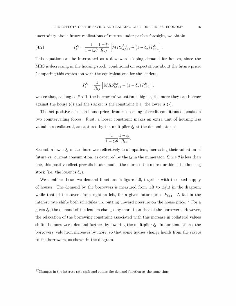
This equation can be interpreted as a downward sloping demand for houses, since the

MRS is decreasing in the housing stock, conditional on expectations about the future price.

Comparing this expression with the equivalent one for the lenders

Pht =

1

Rl,t

�MRS

h,cl,t+1 + (1− δh)P

ht+1

�,

we see that, as long as θ < 1, the borrowers’ valuation is higher, the more they can borrow

against the house (θ) and the slacker is the constraint (i.e. the lower is ξt).

The net positive effect on house prices from a loosening of credit conditions depends on

two countervailing forces. First, a looser constraint makes an extra unit of housing less

valuable as collateral, as captured by the multiplier ξt at the denominator of

1

1− ξtθ

1− ξt

Rb,t.

Second, a lower ξt makes borrowers effectively less impatient, increasing their valuation of

future vs. current consumption, as captured by the ξt in the numerator. Since θ is less than

one, this positive effect prevails in our model, the more so the more durable is the housing

stock (i.e. the lower is δh).

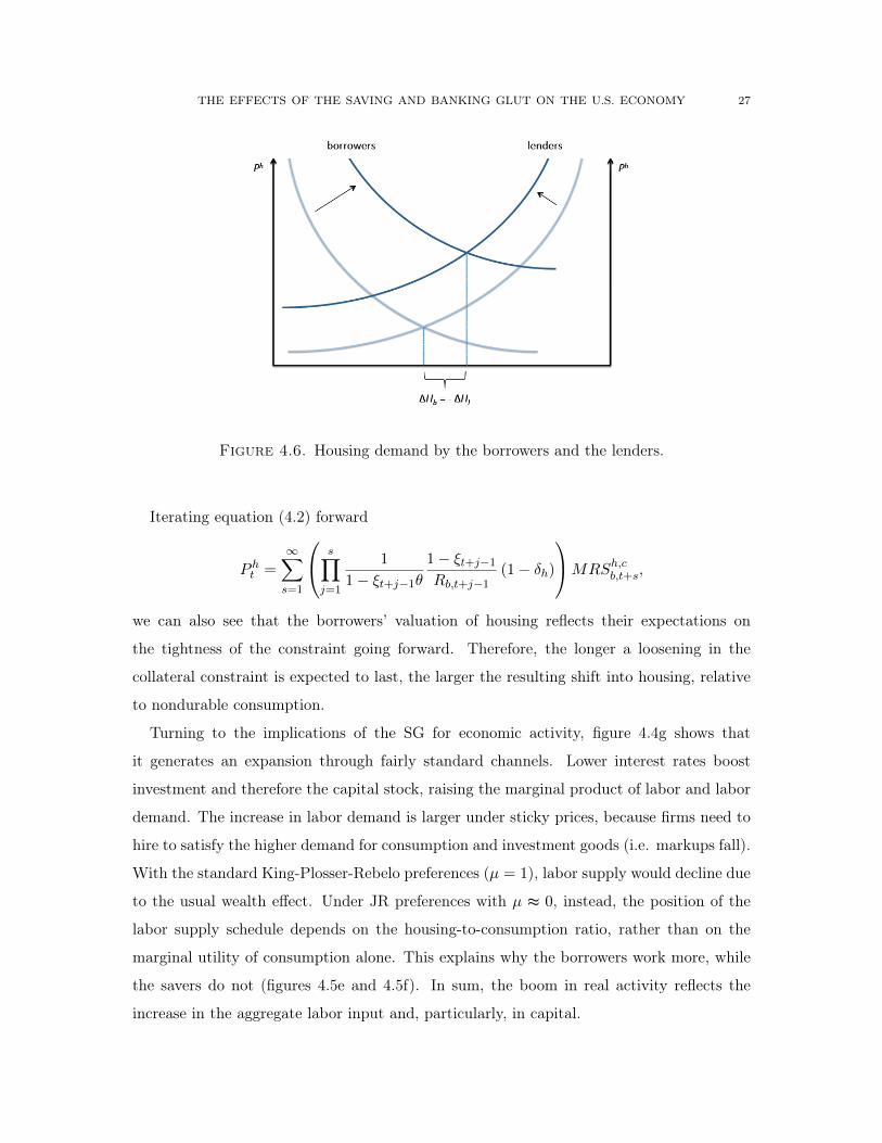
We combine these two demand functions in figure 4.6, together with the fixed supply

of houses. The demand by the borrowers is measured from left to right in the diagram,

while that of the savers from right to left, for a given future price Pht+1. A fall in the

interest rate shifts both schedules up, putting upward pressure on the house price.12 For a

given ξt, the demand of the lenders changes by more than that of the borrowers. However,

the relaxation of the borrowing constraint associated with this increase in collateral values

shifts the borrowers’ demand further, by lowering the multiplier ξt. In our simulations, the

borrowers’ valuation increases by more, so that some houses change hands from the savers

to the borrowers, as shown in the diagram.

12Changes in the interest rate shift and rotate the demand function at the same time.


Figure 4.6. Housing demand by the borrowers and the lenders.

Iterating equation (4.2) forward

Pht =

∞�

s=1

s�

j=1

1

1− ξt+j−1θ

1− ξt+j−1

Rb,t+j−1(1− δh)

MRSh,cb,t+s,

we can also see that the borrowers’ valuation of housing reflects their expectations on

the tightness of the constraint going forward. Therefore, the longer a loosening in the

collateral constraint is expected to last, the larger the resulting shift into housing, relative

to nondurable consumption.

Turning to the implications of the SG for economic activity, figure 4.4g shows that

it generates an expansion through fairly standard channels. Lower interest rates boost

investment and therefore the capital stock, raising the marginal product of labor and labor

demand. The increase in labor demand is larger under sticky prices, because firms need to

hire to satisfy the higher demand for consumption and investment goods (i.e. markups fall).

With the standard King-Plosser-Rebelo preferences (µ = 1), labor supply would decline due

to the usual wealth effect. Under JR preferences with µ ≈ 0, instead, the position of the

labor supply schedule depends on the housing-to-consumption ratio, rather than on the

marginal utility of consumption alone. This explains why the borrowers work more, while

the savers do not (figures 4.5e and 4.5f). In sum, the boom in real activity reflects the

increase in the aggregate labor input and, particularly, in capital.


4.2. Banking glut. In contrast to the saving glut, the banking glut refers to large gross

inflows of foreign capital from advanced economies, mostly Europe, which were matched by

similar outflows, resulting in small net flows and minor changes in the U.S. trade balance

(Shin, 2012). Compared to the portfolio allocation of the SG countries, which was concen-

trated in Treasury and agency debt, the composition of the European gross capital inflows

was more widely spread across asset classes, with a particular concentration in private-label

ABS, corporate bonds and (to a lesser extent) equity (Bernanke et al. 2011). According to

the empirical literature, the higher demand for ABS and corporate bonds from European

investors put downward pressure on the spreads of these securities relative to Treasuries,

despite significant increases in their origination (Bertaut et al. 2011).

Consistent with this description, our model captures the BG as a gross inflow of capital

into the mortgage market, which is not associated with movements in the trade balance.

More specifically, we model the demand by European investment banks for structured

mortgage products, and their associated issuance of credit instruments on the domestic

wholesale credit market, as an increase in the competitive pressure in this market. This

increase in the number of players and in the credit products they issue compresses the

spread between borrowing and lending rates, as shown in equation (2.4) when Nt increases.

Direct evidence on the quantitative implications for spreads of this increased participation

by European banks in the U.S. wholesale credit market is difficult to obtain, since spreads

between mortgage products and funding rates move for many different reasons. Therefore,

our calibration is based on the fact that the spread between mortgage rates and Treasuries

of comparable maturities declined by between 50 and 150 basis points between 2003 and

2007, at the time of the surge of European funds into the market for ABS. Moreover, this

spread compression was more pronounced in mortgage products directly connected with

the subprime boom, which featured prominently in the portfolios of European banks.13

Taking this evidence as a rough guideline, our simulation assumes that in every quarter

between 2003:Q1 and 2006:Q3, agents in the model are surprised with an unanticipated de-

cline in the spread, which they expect to be permanent. Given the ambiguity surrounding

the appropriate choice of a spread measure, our BG experiment assumes a gradual decline13See, for instance, figures 16 and 17 in Bertaut at al. (2011). The portfolio balance model estimated bythese authors suggests that the European purchases of ABS during this period lowered ABS yields by 60basis points. Including the purchases of non-ABS corporate debt, the negative effect on yields reaches 160basis points. However, these estimates do not account for the impact of the increase in supply of theseinstruments, which presumably contributed to reduce these effects on rates.


in the steady state spread by a total of 75 basis points. This number approximately cor-

responds to the decline in the spread between the 30-year mortgage rate and the 10-year

Treasury yield reported by Bertaut et al. (2011) and Bernanke et al. (2011). We also exper-

imented with smaller (50 basis points) and larger declines (1 percent), and found roughly

proportional changes in the model’s dynamics.

Our findings on the implications of the banking glut for the U.S. economy are summarized

in figures 4.7 and 4.8. Faced with a lower nominal (and real) interest rate, the borrowers

reallocate their demand from nondurable consumption towards houses. This shift in demand

puts upward pressure on house prices, which rise by 4% during the first five years. Higher

collateral values allow them to borrow more, and ultimately to increase also the consumption

of nondurable goods. Moreover, the relaxation of the borrowing constraint entails an even

larger decline in the effective interest rate faced by borrowers ( Rt/(1 − ξt)), due to the

current and future expected fall in the multiplier. As a result, the borrowers’ demand for

housing increases substantially more than that for nondurable goods.

Absent any net injections of foreign capital, additional lending from the domestic savers

to satisfy the increased borrowing by the impatient households requires an increase in the

interest rate, which leads them to postpone consumption and investment. This reduction

in the savers’ demand almost exactly counteracts the expansion from the borrowers, re-

sulting in a negligible overall increase in consumption and output. These offsetting effects

of the responses of borrowers and savers on aggregate activity are also a feature of the

closed-economy experiments in Justiniano, Primiceri, and Tambalotti (2012). As in those

experiments, we also find a sizable re-allocation of houses from the borrowers to the savers.

Our simulation of the BG is subject to at least two caveats. First, empirical evidence

suggests that capital inflows from the SG economies also contributed to the reduction in

spreads of mortgage over Treasury yields, perhaps by substantial amounts (Bertaut et al.,

2011, Warnock and Warnock, 2009). Since our model is not well equipped to capture this

effect of the SG, we might be overestimating the impact of the BG relative to the SG.

Second, foreign inflows were not the only factor behind the observed reduction in mortgage

spreads, which is why we view the magnitude of our simulations as only suggestive of the

potential effects of a compression in spreads that might be attributed to the BG channel.

4.3. Saving and banking gluts: a quantitative perspective. This subsection presents

the results of a joint simulation of the SG and the BG. From 1998:Q1 through 2002:Q4,


1998 2000 2002 2004 2006

3.8

3.9

4

4.1

4.2

4.3

a) Real interest rate (borrowing)

1998 2000 2002 2004 2006

6

6.1

6.2

6.3

b) Nominal interest rate (borrowing)

1998 2000 2002 2004 200698.5

99

99.5

100


1998 2000 2002 2004 200699.5

100

100.5

d) Consumption

1998 2000 2002 2004 2006

100

101

102

103

104

e) House price

1998 2000 2002 2004 2006

0.44

0.46

0.48

0.5


1998 2000 2002 2004 2006

99.6

99.8

100

100.2

100.4

100.6

g) GDP

1998 2000 2002 2004 2006

99.6

99.8

100

100.2

100.4

100.6

h) Labor

Figure 4.7. Banking glut: aggregate variables

only the SG is active and the transition paths are identical to those described in section 4.1.

After 2003:Q1, the BG is also active. Given the focus of the previous subsections on the

qualitative mechanisms at play in the model, here we concentrate on the overall quantitative

impact of these international forces, with particular attention to their contribution to the

housing and credit boom.

In our combined experiment, real house prices increase by 17% between 1998 and 2007

(figure 4.9e). Therefore, our results attribute between one-third and one-fourth of the


1998 2000 2002 2004 2006

100

105

110

a) Housing (borrower)

1998 2000 2002 2004 2006

92

94

96

98

100

b) Housing (saver)

1998 2000 2002 2004 200699.5

100

100.5

101

101.5

c) Consumption (borrower)

1998 2000 2002 2004 200698.5

99

99.5

100

100.5

d) Consumption (saver)

1998 2000 2002 2004 200699.5

100

100.5

101

e) Labor (borrower)

1998 2000 2002 2004 2006

99.4

99.6

99.8

100

100.2

100.4

f) Labor (saver)

1998 2000 2002 2004 2006

99.5

100

100.5

g) Real wage (borrower)

1998 2000 2002 2004 200699.5

100

100.5

101

h) Real wage (saver)

Figure 4.8. Banking glut: borrowers and lenders

recent house-price boom to the imbalances vis-a-vis the rest of the world. We regard the

contribution of these international forces as realistic, considering that the literature has

identified a host of domestic factors as important sources of the U.S. housing boom and

bust and of the associated financial crisis, such as changes in the availability of credit on

both the intensive and extensive margin (Mian and Sufi, 2009, Favilukis et al., 2012, Boz

and Mendoza, 2010), loose monetary policy (Taylor, 2008, Ferrero, 2012), or deviations of

house prices from fundamentals (Shiller, 2007).


1998 2000 2002 2004 2006

2.5

2.6

2.7

2.8

a) Real interest rate (lending)

1998 2000 2002 2004 20063.5

4

4.5

b) Nominal interest rate (lending)

1998 2000 2002 2004 2006

100

102

104

106

108

110


1998 2000 2002 2004 2006

100

101

102

103

104

105

d) Consumption

1998 2000 2002 2004 2006100

105

110

115

e) House price

1998 2000 2002 2004 2006

0.45

0.5

0.55


1998 2000 2002 2004 200699.5

100

100.5

101

101.5

102

g) GDP

1998 2000 2002 2004 200699.5

100

100.5

h) Labor

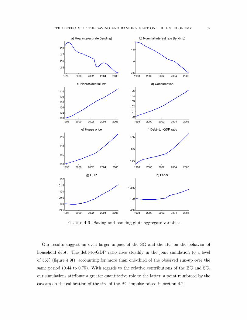
Figure 4.9. Saving and banking glut: aggregate variables

Our results suggest an even larger impact of the SG and the BG on the behavior of

household debt. The debt-to-GDP ratio rises steadily in the joint simulation to a level

of 56% (figure 4.9f), accounting for more than one-third of the observed run-up over the

same period (0.44 to 0.75). With regards to the relative contributions of the BG and SG,

our simulations attribute a greater quantitative role to the latter, a point reinforced by the

caveats on the calibration of the size of the BG impulse raised in section 4.2.


The remaining panels in figure 4.9 plot the behavior of the real interest rate, GDP,

investment and aggregate consumption in the joint experiment. As for most variables in

the model, their transition paths are roughly equal to the sum of the responses in the

two experiments taken in isolation.14The effects on activity are mostly shaped by the SG,

due to the nearly offsetting responses of borrowers and savers to the BG. Investment and

consumption rise considerably above trend, but the expansionary effects on GDP are more

muted, due to the drag coming from the trade deficit.

Overall, the quantitative experiments illustrated above suggest that the sustained current

account deficits run by the United States in the last fifteen years, and to a lesser extent

the gross capital flows into mortgage-backed securities mediated by European banks, had a

sizable impact on the equilibrium of the domestic economy. These flows of goods and assets

reduced interest rates and spreads, and lifted nondurable consumption and house values.

As a result, households’ ability to borrow increased, accounting for more than one third of

the observed surge in debt.

An important qualification to this conclusion is that, given the complexity of the current

model, we took an extremely stylized view of international trade, as an exogenous flow

of imports into the United States from the RoW, with no exports going in the opposite

direction. This simplification is consistent with the two main tenets of the SG hypothesis put

forth by Bernanke (2005). First, that international imbalances are best understood through

the lens of the balance between desired saving and investment—the current account—rather

than through that of the balance between exports and imports—the trade deficit. Second,

that the main source of these imbalances since the late nineties were developments in the

RoW, rather than in the U.S., and in particular the surge in desired saving in emerging

Asia and the Middle East, looking for safe harbor in the United States.

4.3.1. Robustness: supply of new houses. Our baseline model assumes that the supply of

houses expands at the rate of technological progress. This simplifying assumption is not

crucial for our result that the dynamics of foreign capital flows account for between one

fourth and one third of the increase in U.S. house prices and household debt. To illustrate

14The most notable exception is the behavior of household debt, which increases less in the combinedexperiment. The reason is the “zero lower bound” on the multiplier ξt. In the SG experiment, the collateralconstraint does not bind while the trade deficit rises (from 1998:Q1 to 2006:Q3). Since the multiplieris already equal to zero, the reduction in the spread that starts in 2003:Q1 does not have an additionalexpansionary effect on borrowing, because the borrowers are already unconstrained.


this point, we experimented with a more complex version of the model, in which houses

are produced combining a fixed factor (land) and residential investment, as in Davis and

Heathcote (2005). The production of residential investment is subject to adjustment costs

similar to those in equation (2.1), parameterized to approximately match the relative in-

crease in the price and quantity of residential investment observed between 1998 and 2006.

In this version of the model, house prices increase almost as much as in our simpler base-

line specification (close to 14%). Meanwhile, the ratio of residential investment to GDP

experiences a similar increase (roughly 17%) from its steady state level.

5. Concluding Remarks

The United States has been running large trade and current account deficits for more

than twenty years. These deficits grew steadily during the 1990s and 2000s, and fell only

partially following the Great Recession. We studied the quantitative effects of this massive

transfer of resources from the Rest of the World to the U.S. economy, with a particular focus

on its impact on the credit and real estate boom that precipitated the Great Recession.

We did so with help from a dynamic, general equilibrium model that features most of the

now standard ingredients in the DSGE literature. The model also includes borrowing and

lending among heterogeneous households, a non-competitive financial intermediation sector

that charges a spread on borrowing rates, and a stylized foreign sector that lends resources

to the domestic economy in exchange for a promise of more resources in the future. With

these ingredients, we can capture two channels through which global imbalances affected

the U.S. economy. The first channel is the global saving glut popularized by Bernanke

(2005), which we represent as an influx of real resources in the U.S. economy calibrated to

the observed sequence of trade deficits.

The second channel is Shin’s (2012) global banking glut, which refers to the effect of

the gross capital flows intermediated by global (mostly European) banks into the U.S.

mortgage market. The evidence recently collected by Bertaut et al. (2011) suggests that

these gross purchases of mortgage instruments had a significant impact on interest rates

and spreads in the mortgage market, even though they were largely financed on domestic

credit markets, giving rise to virtually no current account imbalance. We capture this

second channel through a compression in the spread charged by financial intermediaries,


associated with the increased competition in the wholesale funding market triggered by the

entry of European banks.

The main finding is that the saving and banking glut together were an important con-

tributor to some of the key macroeconomic developments in the U.S. during the 2000s, and

in particular in the period preceding the financial crisis. In the calibrated model, these

two forces contribute to a large boom in consumption and investment, and account for

between one fourth and one third of the observed run-up in real house prices, and more

than a third in that of household debt. Between the two channels, the saving glut has much

larger effects, since it generates a fall in interest rates for both borrowers and savers that

stimulates their demands, especially of durable goods such as houses. The compression in

spreads with which we capture the banking glut, instead, elicits opposite responses between

borrowers and lenders, leading to smaller effects on aggregate variables.

Our modeling strategy misses at least two potentially important dimensions of the con-

nection between global imbalances and domestic macroeconomic developments. First, the

portfolio composition of the financial flows that mirror the observed trade deficit is irrele-

vant in our model. This is because agents have perfect foresight, and therefore perceive no

risk in the returns of the assets they hold, making them indifferent about the composition

of their portfolio. The main advantage of this strategy is that it focuses on the overall

macroeconomic effect of trade, without having to worry about the underlying financial

flows, which can be difficult to track. The clear disadvantage is that we cannot address the

important issues raised by the strong preference of the saving glut countries, and of China

in particular, for safe U.S. dollar assets. These issues are the focus of Caballero, Farhi,

and Gourinchas (2008) and Mendoza, Quadrini, and Rios-Rull (2009), and of a growing

literature that followed them.

Second, there are no exports and imports explicitly in the model, just resources made

available from the rest of the world for consumption in the U.S., and no structure on

the reason why foreign agents are willing to lend those resources today. Therefore, we

have nothing to say about what happens in the rest of the world, nor about the many

channels through which imports, exports and the exchange rate affect domestic allocations.

Nevertheless, the model provides useful insights on some of the basic mechanisms through

which international imbalances affect a large economy, as well as a reasonable quantification

of their aggregate effects.


References

Acharya, Viral, and Philipp Schnabl. 2009. “Do Global Banks Spread Global Imbalances? The Case of

Asset-Backed Commercial Paper during the Financial Crisis of 2007–2009.” IMF Economic Review, 58(1):

37–73.

Adam, Klaus, Pei Kuang, and Albert Marcet. 2011. “House Price Booms and the Current Account.” NBER

Working Paper no. 17224.

Adrian, Tobias, and Hyun Song Shin. 2010. “The Change in Nature of Financial Intermediation and the

Financial Crisis of 2007-09.” Annual Review of Economics, 2, 603-618.

Ashcraft, Adam B., and Til Schuermann. 2008. “Understanding the securitization of subprime mortgage

credit.” Federal Reserve Bank of New York Staff Reports, 318.

Bernanke, Ben S. 2005. "The Global Saving Glut and the US Current Account Deficit." Sandridge Lecture,

Virginia Association of Economists, April 14, 2005.

Bernanke, Ben S., Carol Bertaut, Laurie Pounder DeMarco, and Steven B. Kamin. 2011. “International

Capital Flows and the Returns to Safe Assets in the United States, 2003–2007." Banque de France Financial

Stability Review, 15: 13–26.

Bertaut, Carol C., Laurie Pounder DeMarco, Steven Kamin, and Ralph W. Tryon. 2011. "ABS Inflows to

the United States and the Global Financial Crisis." International Finance Discussion Papers 1028, Board

of Governors of the Federal Reserve System.

Bertaut, Carol, and Laurie Pounder DeMarco. 2009. “The Financial Crisis and U.S. Cross Border Financial

Flows.” Federal Reserve Bulletin, November 2009: A147–A167.

Bilbiie, Florin O., Fabio Ghironi, and Marc J. Melitz. 2012. “Endogenous Entry, Product Variety, and

Business Cycles.” Journal of Political Economy, 120(2), 304–345.

Boz, Emine, and Enrique G. Mendoza. 2010. “Financial Innovation, the Discovery of Risk, and the U.S.

Credit Crisis.” NBER Working Paper no. 16020.

Brunnermeier, Markus K. 2009. “Deciphering the Liquidity and Credit Crunch 2007-08.” Journal of Eco-

nomic Perspectives, 23(1), 77–100.

Caballero, Ricardo J., and Emmanuel Farhi. 2013. “A Model of the Safe Asset Mechanism (SAM): Safety

Traps and Economic Policy.” NBER Working Paper no. 18737.

Caballero, Ricardo J., Emmanuel Farhi, and Pierre-Olivier Gourinchas. 2008. “An Equilibrium Model of

Global Imbalances and Low Interest Rates.” American Economic Review, 98(1), 358–393.

Caballero, Ricardo, and Arvind Krishnamurthy. 2009. “Global Imbalances and Financial Fragility.” Amer-

ican Economic Review, 99(2), 584-88.

Calvo, Guillermo A. 1983. “Staggered prices in a utility-maximizing framework.” Journal of Monetary

Economics, 12(3): 383–398.

Campbell, Jeffrey R., and Zvi Hercowitz. 2009. “Welfare implications of the transition to high household

debt.” Journal of Monetary Economics, 56(1), 1–16.


Christiano, Lawrence J., Martin Eichenbaum, and Charles L. Evans. 2005. “Nominal rigidities and the

dynamic effects of a shock to monetary policy.” Journal of Political Economy, 113(1), 1–45.

Cúrdia, Vasco, and Michael Woodford. 2010. “Credit spreads and monetary policy.” Journal of Money,

Credit and Banking, 42(1), 3–35.

Davis, Morris A., and Jonathan Heathcote. 2005. "Housing and the business cycle." International Economic

Review, 46(3), 751–784.

Demyanyk, Yuliya, and Van Hemert, Otto. 2011. “Understanding the Subprime Mortgage Crisis.” Review

of Financial Studies, 24(6), 1848–1880.

Devereux, Michael B., and Alan Sutherland. 2011. "Country Portfolios In Open Economy Macro-Models."

Journal of the European Economic Association, 9(2), 337–369.

Duca, John V., John Muellbauer, and Anthony Murphy. 2011. “House Prices and Credit Constraints:

Making Sense of the US Experience.” The Economic Journal, 121(552), 533–551.

Eberly, Janice, Sergio Rebelo, and Nicolas Vincent. 2012. "What explains the lagged investment effect?"

Journal of Monetary Economics, 59(4), 370–380.

Favilukis, Jack, David Kohn, Sydney C. Ludvigson, and Stijn Van Nieuwerburgh. 2013. “International

Capital Flows and House Prices: Theory and Evidence.” Housing and the Financial Crisis, University of

Chicago Press.

Favilukis, Jack, David Kohn, Sydney C. Ludvigson, and Stijn Van Nieuwerburgh. 2012. “Foreign Ownership

of U.S. Safe Assets: Good or Bad?” NYU Working Paper no. FIN-11-057.

Feenstra, Robert C. 2003. “A homothetic utility function for monopolistic competition models, without

constant price elasticity.” Economics Letters, 78(1), 79–86.

Ferrero, Andrea. 2012. "House Price Booms, Current Account Deficits, and Low Interest Rates." Federal

Reserve Bank of New York Staff Reports, 541.

Ferrero, Andrea, Mark Gertler, and Lars EO Svensson. 2010. “Current account dynamics and monetary

policy.” International Dimensions of Monetary Policy, Jordi Gali and Mark Gertler, editors. University of

Chicago Press.

Garcia-Cicco, Javier, Roberto Pancrazi, and Martin Uribe. 2010. “Real Business Cycle in Emerging Coun-

tries? ”American Economic Review, 100(5), 2510–2531.

Garriga, Carlos, Rodolfo E. Manuelli, and Adrian Peralta-Alva. 2012. “A Model of Price Swings in the

Housing Market.” Federal Reserve Bank of St. Louis Working Paper no. 2012-022A.

Gerali, Andrea, Stefano Neri, Luca Sessa, and Federico M. Signoretti. 2010. “Credit and Banking in a

DSGE Model of the Euro Area.” Journal of Money, Credit and Banking, 42(1), 107–141.

Gorton, Gary. 2009. “The Panic of 2007.” Maintaining Stability in a Changing Financial System, Proceed-

ings of the 2008 Jackson Hole Conference, Federal Reserve Bank of Kansas City.

Gourinchas, Pierre-Olivier, and Hélène Rey. 2013. “External Adjustment, Global Imbalances, Valuation

Effects.” Handbook of International Economics, vol. IV, ed. Gita Gopinath, Elhanan Helpman and Kenneth

Rogoff.


Greenspan, Alan. 2005. “Testimony Before the Committee on Banking, Housing, and Urban Affairs,” U.S.

Senate, February 16.

Greenwood, Jeremy, Zvi Hercowitz, and Gregory W. Huffman. 1998. “Investment, capacity utilization, and

the real business cycle.” The American Economic Review, 78(3), 402–417.

Hansen, Gary D. 1985. “Indivisible labor and the business cycle.” Journal of Monetary Economics, 16(3),

309–327.

Himmelberg, Charles, Christopher Mayer and Todd Sinai. 2005. “Assessing High House Prices: Bubbles,

Fundamentals and Misperceptions.” Journal of Economic Perspectives, 19(4), 67–92.

Iacoviello, Matteo. 2005. “House prices, borrowing constraints, and monetary policy in the business cycle.”

The American Economic Review, 95(3), 739–764.

Jaimovich, Nir, and Max Floetotto. 2008. “Firm dynamics, markup variations, and the business cycle.”

Journal of Monetary Economics, 55(7), 1238–1252.

Jaimovich, Nir, and Sergio Rebelo. 2009. “Can News about the Future Drive the Business Cycle?” American

Economic Review, 99(4), 1097–1118.

Julliard, Michel, Douglas Laxton, Peter McAdam, and Hope Pioro. 1998. “An algorithm competition:

First-order iterations versus Newton-based techniques.” Journal of Economic Dynamics and Control, 22:

1291–1318.

Justiniano, Alejandro, Giorgio Primiceri, and Andrea Tambalotti. 2011. “Investment Shocks and the Rel-

ative Price of Investment.” Review of Economic Dynamics, 14(1), 102–121.

Justiniano, Alejandro, Giorgio Primiceri, and Andrea Tambalotti. 2012. “Household Leveraging and

Deleveraging.” NBER Working Paper no. 18941.

Kaplan, Greg, and Giovanni L. Violante. 2011. “A model of the consumption response to fiscal stimulus

payments.” NBER Working Paper no. 17338.

King, Robert G., Charles I. Plosser, and Sergio T. Rebelo. 1988. "Production, growth and business cycles:

I. The basic neoclassical model." Journal of monetary Economics, 21(2), 195–232.

Kiyotaki, Nobuhiro, Alexander Michaelides, and Kalin Nikolov. 2011. “Winners and Losers in Housing

Markets.” Journal of Money, Credit and Banking, 43(2-3), 255–296.

Kiyotaki, Nobuhiro, and John Moore. 1997. "Credit chains." Journal of Political Economy, 105(21), 211–

248.

Krugman, Paul. 2007. “Will There be a Dollar Crisis?” Economic Policy, 22(51), 435–467.

Krusell, Per, and Anthony A. Smith, Jr. 1998. "Income and wealth heterogeneity in the macroeconomy."

Journal of Political Economy, 106(5), 867–896.

McCarthy, Jonathan, and Richard W. Peach. 2004. “Are Home Prices the Next ’Bubble’?” FRBNY

Economic Policy Review, 10(3).

Mian, Atif, and Amir Sufi. 2009. “The Consequences of Mortgage Credit Expansion: Evidence from the

U.S. Mortgage Default Crisis.” Quarterly Journal of Economics, 124(4), 1449–1496.


Mendoza, Enrique G., Vincenzo Quadrini, and José-Victor Ríos-Rull. 2009. "On the welfare implications of

financial globalization without financial development." NBER International Seminar on Macroeconomics

2007, University of Chicago Press, 283–312.

Nakamura, Emi, and Jón Steinsson. "Five facts about prices: A reevaluation of menu cost models." The

Quarterly Journal of Economics, 123(4), 1415–1464.

Neumeyer, Pablo A., and Fabrizio Perri. 2005. “Business cycles in emerging economies: the role of interest

rates.” Journal of Monetary Economics, 52 (2), 345-380.

Obstfeld, Maurice, and Kenneth Rogoff. 2007. “The unsustainable US current account position revisited.”

G7 current account imbalances: Sustainability and adjustment. University of Chicago Press, 339–376.

Obstfeld, Maurice, and Kenneth Rogoff. 2009. “Global Imbalances and the Financial Crisis: Products or

Common Causes.” CEPR Working Paper DP7606.

Obstfeld, Maurice. 2012. “Financial Flows, Financial Crises, and Global Imbalances.” Journal of Interna-

tional Money and Finance, 31(3), 469–480.

Pozsar, Zoltan, Tobias Adrian, Adam Ashcraft, and Hayley Boesky. 2010. “Shadow Banking.” Federal

Reserve Bank of New York Staff Reports, 458.

Roubini, Nouriel, and Brad Setser. 2005. “Will the Bretton Woods 2 Regime Unravel Soon? The Risk of

a Hard Landing in 2005–-2006.” Manuscript, New York University and Oxford University.

Shiller, Robert J. 2007. “Understanding recent trends in house prices and homeownership.” Proceedings,

Federal Reserve Bank of Kansas City : 89–123.

Shin, Hyun Song. 2012. “Global Banking Glut and Loan Risk Premium.” IMF Economic Review, 60(2),

155–192.

Smets, Frank, and Rafael Wouters. 2007. “Shocks and Frictions in US Business Cycles: A Bayesian DSGE

Approach.” American Economic Review, 97(3), 586–606.

Taylor, John B. 2008. “The financial crisis and the policy responses: An empirical analysis of what went

wrong.” A Festschrift in Honour of David Dodge’s Contributions to Canadian Public Policy, Bank of

Canada, 1-18.

Tille, Cédric, and Eric van Wincoop. 2010. "International capital flows." Journal of International Eco-

nomics, 80(2), 157–175.

Warnock, Frank, and Veronica Warnock. 2009. “International Capital Flows and U.S. Interest Rates.”

Journal of International Money and Finance, 28, 903–919.


Federal Reserve Bank of Chicago

E-mail address: [email protected]

Northwestern University, CEPR, and NBER


Federal Reserve Bank of New York


the effects of the saving and banking glut on the u.s. …gep575/sbg5.pdf · fed governor ben...

Documents