the effects of vegetation on stream bank erosion€¦ · dissertation submitted to the faculty ......
TRANSCRIPT
The Effects of Vegetation on Stream Bank Erosion
Theresa M. Wynn
Dissertation submitted to the faculty of the Virginia Polytechnic Institute and State University in partial fulfillment of the requirements for the degree of
Doctor of Philosophy
In
Biological Systems Engineering
Saied Mostaghimi James Burger
Theo Dillaha, III Panayiotis Diplas Conrad Heatwole
May 14, 2004 Blacksburg, Virginia
Keywords: stream bank erosion, riparian buffer, freeze-thaw cycling, desiccation cracking, submerged jet test device, root length density, subaerial processes, erodibility, critical shear stress
Copyright 2004, Theresa M. Wynn
The Effects of Vegetation on Stream Bank Erosion
Theresa M. Wynn
Abstract
Riparian buffers are promoted for water quality improvement, habitat restoration, and
stream bank stabilization. While considerable research has been conducted on the effects of
riparian buffers on water quality and aquatic habitat, little is known about the influence of
riparian vegetation on stream bank erosion.
The overall goal of this research was to evaluate the effects of woody and herbaceous
riparian buffers on stream bank erosion. This goal was addressed by measuring the erodibility
and critical shear stress of rooted bank soils in situ using a submerged jet test device.
Additionally, several soil, vegetation, and stream chemistry factors that could potentially impact
the fluvial entrainment of soils were measured. A total of 25 field sites in the Blacksburg,
Virginia area were tested. Each field site consisted of a 2nd-4th order stream with a relatively
homogeneous vegetated riparian buffer over a 30 m reach. Riparian vegetation ranged from
short turfgrass to mature riparian forest. Multiple linear regression analysis was conducted to
determine those factors that most influence stream bank erodibility and the relative impact of
riparian vegetation.
Results of this research indicated woody riparian vegetation reduced the susceptibility of
stream bank soils to erosion by fluvial entrainment. Riparian forests had a greater density of
larger diameter roots, particularly at the bank toe where the hydraulic stresses are the greatest.
These larger roots (diameters > 0.5 mm) provided more resistance to erosion than the very fine
roots of herbaceous plants. Due to limitations in the root sampling methodology, these results
are primarily applicable to steep banks with little herbaceous vegetation on the bank face, such as
those found on the outside of meander bends.
In addition to reinforcing the stream banks, riparian vegetation also affected soil moisture
and altered the local microclimate. While summer soil desiccation was reduced under deciduous
iii
riparian forests, as compared to herbaceous vegetation, winter freeze-thaw cycling was greater.
As a result, in silty soils that were susceptible to freeze-thaw cycling, the beneficial effects of
root reinforcement by woody vegetation were offset by increased freeze-thaw cycling. Using the
study results in an example application, it was shown that converting a predominately
herbaceous riparian buffer to a forested buffer could reduce soil erodibility by as much as 39% in
soils with low silt contents. Conversely, for a stream composed primarily of silt soils that are
prone to freeze-thaw cycling, afforestation could lead to localized increases in soil erodibility of
as much as 38%. It should be emphasized that the riparian forests in this study were deciduous;
similar results would not be expected under coniferous forests that maintain a dense canopy
throughout the year. Additionally, because dense herbaceous vegetation would likely not
develop in the outside of meander bends where hydraulic shear stresses are greatest, the
reductions in soil erodibility afforded by the herbaceous vegetation would be limited to areas of
low shear stress, such as on gently sloping banks along the inside of meander bends.
As the first testing of this type, this study provided quantitative information on the effects
of vegetation on subaerial processes and stream bank erosion. It also represents the first
measurements of the soil erosion parameters, soil erodibility and critical shear stress, for
vegetated stream banks. These parameters are crucial for modeling the effects of riparian
vegetation for stream restoration design and for water quality simulation modeling.
Grant Information
Funds for this research were provided by Grant No. U-915555-01-0 under the Science to
Achieve Results (STAR) program of the US Environmental Protection Agency, Office of
Research and Development, National Center for Environmental Research; the American
Association of University Women Selected Professions Fellowship; the P.E.O. Scholars Award;
the Virginia Tech General Electric Fund Scholars Program; the Soil and Water Conservation
Society Kenneth E. Grant Research Scholarship;, the American Water Resources Association
Richard A. Herbert Memorial Education Scholarship; the Gene and Ina Mae James Graduate
Scholarship; the Waste Policy Institute Graduate Fellowship; and the Virginia Water Resources
Center William R. Walker Graduate Research Fellowship.

iv
Dedication I wish to dedicate this work to my guys, Benjamin and Jeffrey Wynn, and to remember
those who passed during its development, including Ruth and Paul Schatzle, Johanna Gidley,
Sherry Schatzle, Olga and John Sloboda, and Bernard Gidley.
“The difficulty lies not in the new ideas, but in escaping from the old ones.” - John Maynard Keynes

v
Acknowledgements
I would like to thank my major professor, Saied Mostaghimi, for all his support and
guidance throughout my dissertation program. I would also like to thank Jim Burger, Theo
Dillaha, Panos Diplas, and Conrad Heatwole for their support and input. I am incredibly grateful
to all those who assisted with the extensive field and laboratory work for the “Epic Project,”
including Charles Karpa, Jan Carr, Jeff Wynn, and Julie Jordan, as well as Joe Deal, Adam
Faulkner, Adrian Harpold, Nyeema Harris, Marc Henderson, Leigh-Anne Henry, Leslie
Johnson, Candice Piercy, Sheila Ranganath, and Meghan Siewers. Thank you for suffering
through bad weather, equipment breakdowns, picking roots, and mud pies with me. Lastly, none
of this research would have happened without the generosity and cooperation of numerous
private landowners. Many thanks go to Bob Adams, the Blacksburg Country Club, Paul
Bowyer, Carl Cirillo, Mark Cook, Tammy Decatur, Earl Frith, Joyce Graham, Chuck and Margie
Harris, Mark and Linda McCann, Frank Quinn, Bob Ross, the Town of Blacksburg, Allen
Sisson, and Jim Washington for allowing this research to be conducted on their property. I am
particularly grateful to Earl Frith for loaning me his ATV, without which I would have had
several long, cold, muddy hikes during the winter of 2003.
I would also like to acknowledge the love and support of may family. I want to thank my
guys, Benjamin and Jeffrey Wynn, for enduring the mud, the poison ivy, and the days I couldn’t
play with you. I would also like to thank my parents, Susan and Larry Gidley, for the many
hours of long distance listening and babysitting a sick grandchild. Thank you for your years of
support in its multiple forms. Many thanks also go to Carol and Walter Wynn, for their
encouragement and for filling in when I had to be gone. My family is a blessing beyond
measure.
vi
Table of Contents List of Tables .............................................................................................................................. viii List of Figures ..................................................................................................................................x List of Abbreviations and Symbols.............................................................................................. xiii Chapter 1. Introduction ...................................................................................................................1
1.1. Introduction.......................................................................................................................1 1.2. Goals and Objectives ........................................................................................................3 1.3. Study Design.....................................................................................................................3
Chapter 2. Review of Stream Bank Retreat ....................................................................................6
2.1. Subaerial Processes...........................................................................................................6 2.1.1. Soil Desiccation .......................................................................................................7 2.1.2. Soil Freeze-Thaw Cycling .......................................................................................7 2.1.3. The Significance of Subaerial Processes ...............................................................11
2.2. Fluvial Entrainment ........................................................................................................12 2.2.1. The Effects of Soil Properties on Fluvial Entrainment..........................................13 2.2.2. The Effects of Subaerial Processes on Fluvial Entrainment..................................16 2.2.3. Modeling Fluvial Entrainment...............................................................................18
2.3. Mass Wasting..................................................................................................................29 2.4. Process Dominance.........................................................................................................30 2.5. Basal Endpoint Control...................................................................................................31 2.6. Effects of Vegetation on Stream Bank Stability .............................................................32
2.6.1. Subaerial Processes................................................................................................32 2.6.2. Fluvial Entrainment ...............................................................................................34
2.6.2.1. Effects of Root Density on Soil Erodibility..................................................35 2.6.2.2. Effects of Roots on Soil Properties...............................................................37 2.6.2.3. Root Density in Stream Banks......................................................................39
2.6.3. Mass Wasting.........................................................................................................41 2.6.4. Benefits of Herbaceous vs. Woody Vegetation .....................................................42
2.7. Summary .........................................................................................................................43 Chapter 3. Variation in Root Density Along Stream Banks .........................................................45
3.1. Methods...........................................................................................................................45 3.2. Results and Discussion ...................................................................................................48
3.2.1. Aboveground Vegetation and Soils .......................................................................48 3.2.2. Root Length Density ..............................................................................................50 3.2.3. Root Volume Ratio ................................................................................................56 3.2.4. Regression Analysis...............................................................................................59 3.2.5. Implications for Stream Bank Stability..................................................................61
3.3. Summary and Conclusions .............................................................................................63 Chapter 4. Riparian Vegetation Effects on Freeze-Thaw Cycling and Desiccation of Stream
Bank Soils...................................................................................................................66 4.1. Methods...........................................................................................................................66
4.1.1. Paired Reach Evaluations ......................................................................................66 4.1.2. Freeze-Thaw Cycling Analysis..............................................................................71
vii
4.1.3. Vertical Variations in Subaerial Processes ............................................................73 4.2. Results and Discussion ...................................................................................................73
4.2.1. Paired Reach Evaluations ......................................................................................74 4.2.1.1. Summer Soil Temperature ............................................................................74 4.2.1.2. Summer Soil Water Potential........................................................................82 4.2.1.3. Winter Soil Temperature and Freeze-Thaw Cycling ....................................86 4.2.1.4. Winter Soil Water Potential ..........................................................................92
4.2.2. Regression Analysis of Freeze-Thaw Cycling.......................................................93 4.2.3. Vertical Variations in Subaerial Processes ............................................................98
4.3. Summary and Conclusions .............................................................................................99 Chapter 5. Effects of Vegetation on Stream Bank Erodibility and Critical Shear Stress ...........102
5.1. Methods.........................................................................................................................102 5.1.1. Jet Testing ............................................................................................................102 5.1.2. Soil and Water Characteristics.............................................................................106 5.1.3. Data Analysis .......................................................................................................111
5.2. Results...........................................................................................................................113 5.2.1. Regression Analysis of Overall Data Set.............................................................123 5.2.2. Regression Analysis of Group 1 Data..................................................................129 5.2.3. Regression Analysis of Group 2 Data..................................................................137 5.2.4. Regression Analysis of Group 3 Data..................................................................139
5.3. Discussion.....................................................................................................................144 5.3.1. Bulk Density ........................................................................................................144 5.3.2. Moisture Content and Aggregate Stability ..........................................................145 5.3.3. Soil Chemistry .....................................................................................................146 5.3.4. Soil Freezing ........................................................................................................147 5.3.5. Root Density ........................................................................................................148 5.3.6. Example Application of Study Results ................................................................149 5.3.7. Evaluation of the Jet Test Device ........................................................................152
5.4. Summary and Conclusions ...........................................................................................155 Chapter 6. Overall Summary and Conclusions...........................................................................160
6.1. Summary .......................................................................................................................160 6.2. Conclusions...................................................................................................................165 6.3. Research Contributions.................................................................................................167
References Cited ..........................................................................................................................168 Appendix A. Field Research Site Information ..........................................................................182 Appendix B. Aboveground Vegetation .....................................................................................197 Appendix C. Soils Data from Composite Cores........................................................................202 Appendix D. Root Length Density and Root Volume Ratio.....................................................205 Appendix E. Pictures of Paired Sites ........................................................................................216 Appendix F. Freeze-Thaw Regression Analysis Data ..............................................................223 Appendix G. Submerged Jet Test Device..................................................................................226 Appendix H. Data Used in the Soil Erodibility and Critical Shear Stress Analysis..................230 Vita ..............................................................................................................................255

viii
List of Tables
Table 3.1. Aboveground vegetation quantities for forested and herbaceous riparian buffers, southwest, Virginia......................................................................................49
Table 3.2. Median root length density (RLD) by root diameter and depth for forested and herbaceous riparian buffers in southwest Virginia.............................................55
Table 3.3. Median root volume ratio (RVR, %) by root diameter and depth for forested and herbaceous riparian buffers in southwest Virginia.............................................58
Table 3.4. Root length density regression equations for Appalachian headwater stream banks with forested and herbaceous riparian buffers................................................60
Table 3.5. Root volume ratio regression equations for Appalachian headwater stream banks with forested and herbaceous riparian buffers................................................62
Table 4.1. Characteristics of paired field sites. ..........................................................................67 Table 4.2. Average daily soil temperature and water potential conditions for summer
and winter at paired sites, southwest, Virginia. ........................................................79 Table 4.3. Freeze-thaw cycling regression equations using normalized independent
variables for Appalachian headwater streams in southwest Virginia .......................95 Table 4.4. Difference between upper and lower bank summer mean daily soil water
potential in Appalachian headwater streams in southwest Virginia .........................98 Table 5.1. Soil tests conducted and methodology used. ..........................................................107 Table 5.2. Activities of various minerals. ................................................................................110 Table 5.3. Mean, median and range of soil properties from individual jet test runs along
headwater streams in southwest Virginia. ..............................................................121 Table 5.4. Mean, median and range of root length density and root volume ratio from
individual jet test runs along headwater streams in southwest Virginia. ................121 Table 5.5. Mean, median and range of water physical and chemical characteristics for
individual jet test runs in headwater streams in southwest Virginia.......................122 Table 5.6. Mean, median and range of soil chemistry and texture for upper and lower
banks from composite samples along headwater streams in southwest Virginia. ..................................................................................................................122
Table 5.7. Single explanatory variables for soil erodibility, Kd with all data .........................124 Table 5.8. Single explanatory variables for soil critical shear stress, �c with all data ...........125 Table 5.9. Statistically significant differences in median soil properties between the
soil groups for stream bank soils along headwater streams in southwest Virginia ...................................................................................................................131
Table 5.10. Single explanatory variables for soil erodibility, Kd with Group 1 soils ...............132 Table 5.11. Single explanatory variables for soil critical shear stress, �c with Group 1
soils .........................................................................................................................136 Table 5.12. Single explanatory variables for soil erodibility, Kd with Group 3 soils ...............141 Table 5.13. Single explanatory variables for soil critical shear stress, �c with Group 3
soils .........................................................................................................................143 Table A1. General research site information. ..........................................................................183 Table B1. Aboveground vegetation density. ...........................................................................198 Table B2. Aboveground vegetation.........................................................................................199 Table C1. Composite core soils data. ......................................................................................203
ix
Table D1. Root length density. ................................................................................................206 Table D2. Root volume ratio. ..................................................................................................211 Table F1. Freeze-thaw regression data....................................................................................224 Table F2. Freeze-thaw regression equations with field data...................................................225 Table H1. Individual jet test data with soil physical data. .......................................................231 Table H2. Stream chemistry data for individual jet tests.........................................................236 Table H3. Root density for individual jet tests. .......................................................................240 Table H4. Average jet test soil physical data...........................................................................245 Table H5. Average jet test soil and stream water chemical data. ............................................247 Table H6. Data transformations for jet test analysis................................................................249 Table H7. Pearson’s correlation coefficients and p-values for entire averaged jet test
data set ....................................................................................................................250 Table H8. Pearson’s correlation coefficients and p-values for Group 1 soils .........................251 Table H9. Pearson’s correlation coefficients and p-values for Group 2 soils .........................252 Table H10. Pearson’s correlation coefficients and p-values for Group 3 soils .........................253 Table H11. Definition of parameter variable names for Tables H7-H10. .................................254
x
List of Figures
Figure 1.1 Location of research field sites, southwestern Virginia, USA....................................5 Figure 2.1 Soil cracking due to desiccation at site ST3 ...............................................................9 Figure 2.2. Shields diagram.........................................................................................................19 Figure 2.3. Critical shear stress versus sodium adsorption ratio for different salt
concentrations (N) and dielectric dispersion values .................................................23 Figure 2.4. The rate of change of erosion rate versus the critical shear stress for
undisturbed cohesive soils using distilled water as the eroding fluid.......................24 Figure 2.5. Schematic of submerged jet testing device...............................................................27 Figure 2.6. Plot of H* versus T* with best fit regression line for site ST2, test 1, upper
bank...........................................................................................................................30 Figure 2.7. Bank failure schematic..............................................................................................31 Figure 3.1. Root length density with depth and diameter class for herbaceous and
forested stream banks in southwest Virginia ............................................................51 Figure 3.2. Changes in root length density from bank face for herbaceous and woody
vegetation on both vegetated and cut stream banks in southwest Virginia. .............53 Figure 3.3. Median root length density with depth for forested and herbaceous riparian
buffers, southwest Virginia.......................................................................................54 Figure 3.4. Median root volume ratio with depth for forested and herbaceous riparian
buffers in southwest Virginia....................................................................................57 Figure 4.1. Soil temperature and water potential sensor placement in stream banks..................68 Figure 4.2. Installation of site SC6..............................................................................................69 Figure 4.3. Monthly air temperature and precipitation for Blacksburg, Virginia for May
2002 through April 2003...........................................................................................74 Figure 4.4 Soil desiccation cracking at site ST3. .......................................................................75 Figure 4.5. Stream bank degradation at site TC7 resulting from severe soil desiccation ...........75 Figure 4.6. Needle ice in the stream bank toe at site SC7...........................................................76 Figure 4.7. Loose soil at site TC4 resulting from freeze-thaw cycling. ......................................77 Figure 4.8. Accumulation of upper bank soil at mid-bank as a result of freeze-thaw
cycling at site ST3.....................................................................................................77 Figure 4.9. Erosional notch observed at site ST3........................................................................78 Figure 4.10. Range in summer upper bank soil temperature as a function of vegetation
type for Appalachian headwater streams in southwest Virginia...............................80 Figure 4.11. Range in summer lower bank soil temperature as a function of vegetation
type for Appalachian headwater streams in southwest Virginia...............................81 Figure 4.12. Effect of solar radiation on stream bank soil temperature for an Appalachian
headwater stream in southwest Virginia. ..................................................................82 Figure 4.13. Effect of growing season length on upper bank summer soil temperatures,
East Fork of the Little River, near Pilot, Virginia.....................................................83 Figure 4.14. Summer stream bank soil water potential along Sinking Creek near
Newport, Virginia for Herbaceous (H) and Forest (F) sites. ....................................84 Figure 4.15. Range in winter upper bank soil temperature as a function of vegetation type
for Appalachian headwater streams in southwest Virginia.......................................87
xi
Figure 4.16. Range in winter lower bank soil temperature as a function of vegetation type for Appalachian headwater streams in southwest Virginia.......................................88
Figure 4.17. Loose soil on bank face of SC7 due to freeze-thaw cycling. ...................................90 Figure 4.18. Effect of dense groundcover on soil temperatures for a headwater stream in
southwest Virginia ....................................................................................................91 Figure 4.19. Dense winter cover on stream bank at site SC6. ......................................................94 Figure 5.1. Multiangle submerged jet testing device ................................................................103 Figure 5.2. Jet test setup at heavily wooded site, TC4. .............................................................105 Figure 5.3. Prepared bank surface prior to jet testing. ..............................................................106 Figure 5.4. Bentonite seal around tank edge following test run................................................107 Figure 5.5. The effect of test duration on the soil erodibility coefficient..................................115 Figure 5.6. The effect of test duration on the soil critical shear stress......................................116 Figure 5.7. Typical scour plots from jet testing. .......................................................................117 Figure 5.8. Eroded aggregates at bottom of jet test tank...........................................................118 Figure 5.9. Relationship between average stream bank soil erodibility and critical shear
stress........................................................................................................................119 Figure 5.10. Classification of stream bank materials following Hanson and Simon
(2001)......................................................................................................................120 Figure 5.11. The effects of big root volume (2 mm < diameter < 20 mm) and bulk
density on soil erodibility for headwater stream banks in southwestern Virginia. ..................................................................................................................128
Figure 5.12. Relationship between soil erodibility and the number of freeze-thaw cycles for Group 1 soils .....................................................................................................134
Figure 5.13. The effects of big root volume (2 mm < diameter < 20 mm) and bulk density on soil erodibility of Group 3 soils.............................................................142
Figure 5.14. Soil core holes exposed at site ST3 during February 2003 flood...........................153 Figure 5.15. Exposed roots at site SR1. ......................................................................................155 Figure A1. Site EL1 on the East Fork of the Little River. ........................................................184 Figure A2. Site EL2 on the East Fork of the Little River. ........................................................184 Figure A3. Site EL3 on the East Fork of the Little River. .......................................................185 Figure A4. Site EL4 on the East Fork of the Little River. ........................................................185 Figure A5. Site NR1 on the North Fork of the Roanoke River.................................................186 Figure A6. Site NR2 on the North Fork of the Roanoke River.................................................186 Figure A7. Site SC1 on Sinking Creek. ....................................................................................187 Figure A8. Site SC2 on Sinking Creek. ....................................................................................187 Figure A9. Site SC3 on Sinking Creek. ....................................................................................188 Figure A10. ......................................................................................... Site SC4 on Sinking Creek. 188 Figure A11. Site SC5 on Sinking Creek. ....................................................................................189 Figure A12. Site SC6 on Sinking Creek. ....................................................................................189 Figure A13. Site SC7 on Sinking Creek. ....................................................................................190 Figure A14. Site SR1 on the South Fork of the Roanoke River. ................................................190 Figure A15. Site SR3 on the South Fork of the Roanoke River. ................................................191 Figure A16. Site SR4 on the South Fork of the Roanoke River. ................................................191 Figure A17. Site ST1 on Stroubles Creek...................................................................................192 Figure A18. Site ST2 on Stroubles Creek...................................................................................192 Figure A19. Site ST3 on Stroubles Creek...................................................................................193
xii
Figure A20. Site ST4 on Stroubles Creek...................................................................................193 Figure A21. Site TC1 on Toms Creek. .......................................................................................194 Figure A22. Site TC2 on Toms Creek. .......................................................................................194 Figure A23. Site TC4 on Toms Creek. .......................................................................................195 Figure A24. Site TC6 on Toms Creek. .......................................................................................195 Figure A25. Site TC7 on Toms Creek. .......................................................................................196 Figure E1. Site EL4 in summer. ...............................................................................................217 Figure E2. Bank face at EL3 in winter. ....................................................................................217 Figure E3. Site EL4 in summer. ...............................................................................................218 Figure E4. Site EL4 in winter looking downstream. ................................................................218 Figure E5. Site SC6 in summer. ...............................................................................................219 Figure E6. Site SC6 in winter looking upstream. Site on left..................................................219 Figure E7. Site TC1 looking upstream. ....................................................................................220 Figure E8. Riparian buffer at site TC1 .....................................................................................220 Figure E9. Datalogger enclosure at site TC1 following storm event on 2/22/03. ....................221 Figure E10. Site TC2 (on right) looking downstream in winter. ................................................221 Figure E11. Site TC2 in summer. ...............................................................................................222 Figure G1. Multiangle submerged jet testing device ................................................................227 Figure G2. Placing submergence tank.......................................................................................228 Figure G3. Jet test setup at site EL1..........................................................................................228 Figure G4. Filling tank with water prior to start of jet test .......................................................229 Figure G5. Taking point gage reading on bank.........................................................................229
xiii
List of Abbreviations and Symbols
∆T.............................................................................................................. freezing point depression γ ......................................................................................................................... unit weight of water ρ ............................................................................................................................... Spearman’s rho σ ................................................................................................standard deviation of soil grain size σNT.............................................................................................standard deviation of soil grain size τ.......................................................................................................Kendalls correlation coefficient τc................................................................................................................... soil critical shear stress τc,NT ................................................................ normalized and transformed soil critical shear stress τf .............................................................................................................. applied fluvial shear stress τo ....................................................................................................... maximum applied shear stress µS....................................................................................................................................microsemin %clay....................................................................................................................... soil clay content %sand......................................................................................................................soil sand content a............................................................................................................................... fitted coefficient ADF..............................................................................................................average duration frozen ADFNT ........................................................... normalized and transformed average duration frozen AS ........................................................................................................................ aggregate stability ASNT....................................................................... normalized and transformed aggregate stability ASAE ..........................................................................American Society of Agricultural Engineers ASCE ..................................................................................... American Society of Civil Engineers ASTM ......................................................................... American Society for Testing and Materials b................................................................................................................................. fitted exponent BD........................................................................................................................... soil bulk density BDNT .........................................................................normalized and transformed soil bulk density BMP ......................................................................................................... best management practice BRLD............................................................................................................ big root length density BRVR...............................................................................................................big root volume ratio BRVRNT .............................................................normalized and transformed big root volume ratio BSA........................................................................................................................... basal stem area BSAN...................................................................................................... normalized basal stem area C................................................................................................................ jet test nozzle coefficient Cd......................................................................................................................jet diffusion constant Ca ..........................................................................................................................................calcium CL ......................................................................................................................................clay loam do ...................................................................................................................jet test nozzle diameter D................................................................................................................................... root diameter D50 ....................................................................................................................median soil diameter D50,NT..................................................................normalized and transformed median soil diameter Dr...............................................................................................................................dispersion ratio DegreesN .......................................................................................... normalized degrees from north DepthN........................................................................... normalized average baseflow stream depth E ......................................................................................................................................erosion rate
xiv
Ei .......................................................................................................................... initial erosion rate EC ..................................................................................................................electrical conductivity ElevN ......................................................................................................... normalized site elevation ELx............................................................................................. East Fork of the Little River Site x FRLD ........................................................................................................... fine root length density FRLD NT ......................................................... normalized and transformed fine root length density FTC ....................................................................................................................freeze-thaw cycling FTCNT...................................................................normalized and transformed freeze-thaw cycling FTCs.....................................................................................................................freeze-thaw cycles Grass .....................................................................................................................grass dry biomass GrassN ................................................................................................normalized grass dry biomass h........................................................................................................................ jet test pressure head He ..............................................................................................................jet maximum scour depth Hi ................................................................................................ jet initial height above soil surface Hp ......................................................................................................................... jet test core length hr ................................................................................................................................................ hour Kd ............................................................................................................. soil erodibility coefficient Kd,NT ...........................................................normalized and transformed soil erodibility coefficient Kf................................................................................. freezing point depression constant for water KIF ........................................................................................................... potassium intensity factor KIF NT......................................................... normalized and transformed potassium intensity factor LS.................................................................................................................................... loamy sand m...................................................................................................................... soil solution molality M..........................................................................................................................................molarity MC .................................................................................................soil antecedent moisture content MCNT................................................normalized and transformed soil antecedent moisture content MDF............................................................................................................. median duration frozen NRx.................................................................................... North Fork of the Roanoke River Site x NRCS ................................................................................Natural Resources Conservation Service O.......................................................................................................... clay alumina octahedra sheet OC.......................................................................................................... soil organic carbon content OCNT ........................................................normalized and transformed soil organic carbon content PCA................................................................................................... principle components analysis PI ...............................................................................................................................plasticity index PSA .................................................................................................................. particle size analysis PW....................................................................................................... pore water salt concentration R................................................................................................................. channel hydraulic radius RAR ............................................................................................................................ root area ratio RDAM..................................... relative difference between average and median freezing durations RDAMNT ... normalized and transformed rel. diff. between average and median freezing durations RLD..................................................................................................................... root length density RVR .......................................................................................................................root volume ratio Sand.........................................................................................................................soil sand content SandNT ...................................................................... normalized and transformed soil sand content S ......................................................................................................channel energy grade line slope Sv .......................................................................................................................... soil shear strength
xv
SAP .....................................................................................................................subaerial processes SAR............................................................................................................. sodium adsorption ratio S:C..........................................................................................................................soil silt:clay ratio S:CNT ........................................................................normalized and transformed soil silt:clay ratio S+C .............................................................................................. sum of soil silt and clay fractions S+CN ......................................................................... normalized sum of soil silt and clay fractions SCx................................................................................................................... Sinking Creek Site x SCV...................................................................................................................shrub crown volume SG ...................................................................................................................... soil specific gravity SGNT.....................................................................normalized and transformed soil specific gravity SiL......................................................................................................................................silty loam SiltN ...................................................................................................... normalized soils silt content SL.................................................................................................................................... sandy loam SRx..................................................................................... South Fork of the Roanoke River Site x ST.............................................................................................................................soil temperature STx.................................................................................................................Stroubles Creek Site x SWEC ............................................................. ratio of soil to water specific electrical conductivity SWP ....................................................................................................................soil water potential SWpH.................................................................................................... ratio of soil pH to water pH SWpH NT ................................................. normalized and transformed ratio of soil pH to water pH t .................................................................................................................................... time of scour T .............................................................................................................. clay silica tetrahedra sheet TCx ......................................................................................................................Toms Creek Site x TD ................................................................................................................................... tree density TDF................................................................................................................... total duration frozen TGC...................................................................................................total groundcover dry biomass TMDL ...................................................................................................... total maximum daily load TS........................................................................................................... soil total salt concentration TS NT......................................................... normalized and transformed soil total salt concentration Uo .........................................................................................................................jet velocity in core VFRLD ................................................................................................ very fine root length density VIF .............................................................................................................. variance inflation factor WDC .............................................................................................................wetting-drying cycling WDCs..............................................................................................................wetting-drying cycles WGC .............................................................................................woody groundcover dry biomass WGCN ........................................................................ normalized woody groundcover dry biomass WidthN...........................................................................normalized average stream baseflow width WT ............................................................................................................stream water temperature WT NT ..........................................................normalized and transformed stream water temperature x.................................................................................................................. depth down stream bank y...................................................................................................total root length density at depth x

1
Chapter 1. Introduction
1.1. Introduction
Sediment is a primary cause of water quality impairment, causing roughly $16 billion in
damage annually in North America (USEPA, 2002; ARS, 2003). While considerable effort has
been directed toward developing best management practices (BMPs) to reduce erosion from
agricultural and urban lands, another major source of sediment, stream channel erosion, has
largely been ignored. Studies have shown that sediment from stream banks can account for as
much as 90% of watershed sediment yields (Kirkby, 1967; Grissinger et al., 1981a; Roseboom
and Russell, 1985; Trimble, 1997a; Lawler et al., 1999; Prosser et al., 2000). In addition to water
quality impairment, stream bank erosion impacts floodplain residents, riparian ecosystems,
bridges, and other stream-side structures (ASCE, 1998a). Bank erosion rates of 1.5 - 1100
m/year have been documented (Simon et al., 2000). In 1981, the U.S. Army Corps of Engineers
estimated that 575,000 stream bank miles were actively eroding, requiring an average annual
treatment cost of $1.1 billion (USACE, 1981).
Riparian buffers are a recognized BMP for water quality improvement and stream
restoration (Dillaha et al., 1989; Lowrance et al., 1995; Correll, 1996; Daniels and Gilliam,
1996). A riparian buffer is commonly defined as a band of vegetation adjacent to a body of
water that forms the transition between aquatic and upland environments (Palone and Todd,
1997). In the eastern U.S., riparian vegetation ranges from grasses and forbs to shrubs and
mature forests. Research has shown that grass and forested riparian buffers are effective at
removing contaminants from overland flow and shallow groundwater (Lowrance et al., 1995).
Forested buffers are also critical for maintaining aquatic ecosystems in eastern streams (Palone
and Todd, 1997).
In addition to water quality and habitat benefits, riparian vegetation has a significant
impact on stream stability and morphology (Mosley, 1981; Hey and Thorne, 1986; Gregory and
Gurnell, 1988; Thorne and Osman, 1988; USACE, 1994; Abernethy and Rutherfurd, 2000). As
such, it has become an integral part of stream restoration designs (Henderson, 1986; Shields, Jr.
et al., 1995; Jennings et al., 1999). While the importance of vegetation in stream bank stability is
widely acknowledged, the impacts are complex, poorly understood, and have yet to be quantified
2
(Mosley, 1981; Murgatroyd and Ternan, 1983; Hickin, 1984; Heede and Rinne, 1990; ASCE,
1998a; Abernethy and Rutherfurd, 2000; Thorne et al., 1997). Current stream restoration designs
are based on empirical methods and standardized practices (Gregory and Gurnell, 1988;
O'Laughlin, 1995; FISRWG, 1998; Jennings et al., 1999; VeriTech, Inc., 1999; Hession, 2001).
A better understanding of the effects of vegetation on the processes involved in stream bank
retreat is necessary for improved stream restoration design and riparian management (Abernethy
and Rutherfurd, 1998). As Bohn (1989) stated “…by understanding the processes which weaken
stream banks, land managers can develop streamside management strategies which reduce
stream bank vulnerability and favor functional stability.”
Stream restoration designs also need to be assessed for their long-term success,
particularly in the face of future landuse changes (Horwitz et al., 2000). Existing models of
stream morphology provide little assistance in the assessment of stream restoration projects
because they do not consider the effects of vegetation (ASCE, 1998b). Additionally, as states are
required to develop management plans with Total Maximum Daily Loads (TMDLs) for listed
impaired waters, there will be a need to quantify all significant sources of sediment within
watersheds and to determine the effect of proposed controls.
Vegetation type also plays a key role in channel morphology (Hey and Thorne, 1986;
Hession, 2001). Several researchers have noted that streams were 2 - 2.5 times wider with
forested riparian buffers than with grass buffers (Zimmerman et al., 1967; Clifton, 1989;
Sweeney, 1992; Davies-Colley, 1997; Trimble, 1997b; Hession et al., 2000). This information
has prompted some researchers to predict that watershed afforestation may lead to increased
sediment yields (Murgatroyd and Ternan, 1983; Smith, 1992; Davies-Colley, 1997; Trimble,
1997b; Davies-Colley, 2000; Lyons et al., 2000) and that stream sediment yields could be
reduced by converting riparian forests to grass (Trimble, 1997b). Alternatively, others have
shown that forested streams are narrower than streams with herbaceous buffers (Gregory and
Gurnell, 1988; Rosgen, 1996). A study in British Columbia determined major bank erosion was
30 times more prevalent on nonforested versus forested meander bends (Beeson and Doyle,
1995). In a study following the 1993 Kansas floods, Geyer et al. (2000) showed that areas with
herbaceous buffers experienced an average of 24 m of bank erosion while areas with forested
buffers experienced soil deposition. Hession (2001) hypothesized these conflicting findings on
the effects of vegetation on channel form are the result of site-specific differences in watershed
3
characteristics, such as vegetation density and type, soils, flow regimes, slopes, geology, stream
size, and disturbance history. Ultimately, further studies are necessary to evaluate the impact of
vegetation type on stream morphology for effective stream and river management (Mosley,
1981; Gregory and Gurnell, 1988; Heede and Rinne, 1990; Thorne, 1990; Abernethy and
Rutherfurd, 1998; ASCE, 1998a; Horwitz et al., 2000; Lyons et al., 2000; Hession, 2001; Simon
and Collison, 2001).
1.2. Goals and Objectives
The overall goal of this research is to compare the effects of woody and herbaceous
vegetation on stream bank erosion. This research is intended to evaluate the effects of vegetation
on the susceptibility of stream bank material to fluvial entrainment. The results of this research
will provide quantitative information for the design of stream restoration projects, will assist with
the development of sediment TMDLs, and will provide guidance to watershed managers in the
selection of riparian vegetation. Specific objectives include the following:
1. Quantify root-length density with depth in stream banks as a function of riparian buffer vegetation type and density;
2. Determine the effect of vegetation type on freeze-thaw and desiccation activity in stream bank soils; and
3. Use in situ erodibility measurements to evaluate the relative effects of vegetation type and root-length density on the erodibility of stream banks.
1.3. Study Design
A stable stream is one where the flow regime and sediment supply are in a state of quasi-
equilibrium over a period of decades or centuries (Schumm and Lichty, 1965). These systems
are often referred to as “graded” or “in regime” (Mackin, 1948; Leopold and Maddock, 1953;
Wolman, 1955; Leopold et al., 1964; Ackers, 1992; ASCE, 1998a). While stream bank erosion
may occur in stable streams, particularly on the outside of meander bends, this erosion is
balanced by deposition on the opposite bank, such that graded streams maintain their channel
form over long periods of time. Several models are used to predict the geometry of stable
streams for engineering design. Examples include empirical (regime and power law), extremal
hypothesis, or mechanistic (tractive force) methods (ASCE, 1998a). Recent research and
modeling efforts in the design of stable stream channels have utilized the mechanistic tractive
4
force method to evaluate stream stability (Osman and Thorne, 1988; Simon et al., 1999;
Langendoen, 2000). This research assumes this mechanistic tractive force model to address the
role of vegetation in stream bank stability by assessing the impact of riparian vegetation on two
processes involved in stream bank retreat, subaerial processes and bank erosion (fluvial
entrainment).
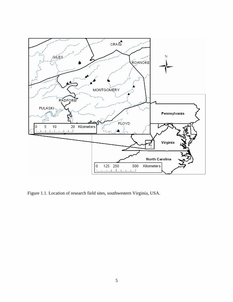
Twenty-five field sites were established along streams near the Town of Blacksburg in
southwest Virginia (37o15’ N, 80o25’ W; Figure 1.1). Each field site consists of a 2nd-4th order
stream with a relatively homogeneous vegetated riparian buffer over a stream reach of 30 meters.
The study focused on a 10 m wide buffer area, as measured from the edge of the baseflow water
level. Average baseflow depths were 20 - 50 cm, while bank exposure ranged from 65 cm to 225
cm and bank angles were 30o-90o. Baseflow channel widths varied from 3 m to 24 m, with
drainage areas of 9 - 322 km2. Bed materials ranged from sand to boulders. The riparian
vegetation varied from short turfgrass to mature forests, representing the full range of possible
vegetation types.
This area lies in the Appalachian Mountains in southwestern Virginia and the climate is
typical of temperate mountain regions. Elevations range from 350 m to 900 m NGVD29 and
average annual rainfall is about 1100 mm. Rainfall has a relatively even distribution throughout
the year, although slightly more precipitation occurs in spring and droughts are common in late
July and August. Individual site information is detailed in Appendix A with photographs of each
site.
To address the research objectives, three separate studies were undertaken. The first
study measured root density and distribution in riparian stream banks as a function of riparian
vegetation type and density, while the second study evaluated the effects of riparian vegetation
on stream bank soil temperature (ST) and moisture regimes. The third and final study quantified
stream bank soil erodibility and critical shear stress in situ. The effects of aboveground
vegetation density, root density, soil freeze-thaw cycling, and soil chemical and physical
properties on stream bank erosion were evaluated. The methodology, results, and discussion for
each of the studies is presented in separate chapters.
5
Figure 1.1. Location of research field sites, southwestern Virginia, USA.
6
Chapter 2. Review of Stream Bank Retreat
Changes in watershed landuse, river regulation, or channel engineering may change
stream flow and/or sediment regimes and these may trigger instabilities in stream form. Stream
bank erosion occurs by a combination of three processes: subaerial processes, fluvial
entrainment, and mass wasting (Lawler, 1992; Lawler, 1995). Each of these processes is
discussed in the following chapter. Also considered are the effects of vegetation on these three
processes and methods to model stream bank erosion.
To provide clarity for the following discussions, the author adopted the terminology
proposed by Lawler et al. (1997). Specifically, the terms “erosion” and "fluvial entrainment" are
used to describe the detachment, entrainment, and removal of individual soil particles or
aggregates from the stream bank face by the hydraulic forces occurring during flood events. The
phrases “bank failure” or "mass wasting" denote the physical collapse of all or part of the stream
banks as a result of geotechnical instabilities. Bank erosion and bank failure commonly work in
concert to produce “bank retreat” or the net recession of the stream bank. Two additional terms,
soil “erodibility” and “critical shear stress” describe, respectively, the ease with which soil is
removed from the bank face and the hydraulic shear stress at which significant erosion is
initiated. As will be discussed in the following sections, these parameters are used in the excess
stress equation and are primarily dependent on soil properties (Hanson and Simon, 2001).
2.1. Subaerial Processes
Subaerial processes (SAP) are climate-related phenomena that serve to reduce soil
strength (e.g. frost heave, soil desiccation; Thorne, 1982). Controlled mainly by climatic
conditions, SAP are largely independent of flow. They dominate stream bank retreat in the
upper reaches of river systems, delivering soil directly to the stream channel and making the
banks more vulnerable to flow erosion by reducing the packing density of soils and destroying
imbrication (Thorne and Tovey, 1981; Abernethy and Rutherfurd, 1998). Measured average
erosion rates due exclusively to SAP range from 13 mm/yr (Prosser et al., 2000) to 40 mm/yr
with peaks as high as 181 mm/yr (Couper and Madock, 2001). Subaerial processes are
7
sometimes described as “preparatory processes” as they increase soil erodibility (Wolman, 1959;
Lawler, 1993).
2.1.1. Soil Desiccation
Contrasting views exist regarding the effects of desiccation on soil erodibility. Several
researchers have shown that drier soils are more resistant to fluvial entrainment (Wolman, 1959;
Knighton, 1973; Hooke, 1979). Soil desiccation has been shown to increase soil strength:
Nearing et al. (1988) stated soil suction increases soil stability by increasing the effective stress
in soils. Soil drying can also cause soil cementation due to the precipitation of calcium
carbonates, silica, gypsum, or iron oxides (Lehrsch, 1998).
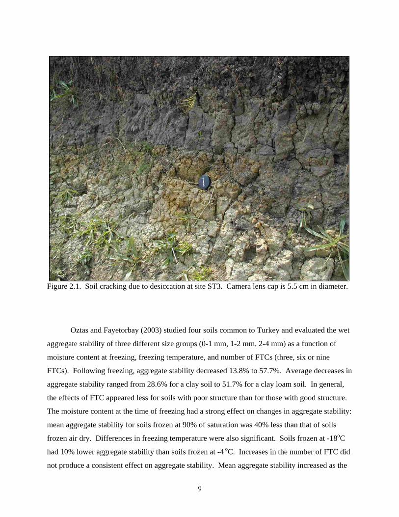
Alternatively, soil desiccation can decrease soil strength. Stream bank desiccation
creates peds and crumbs, which have little resistance to erosion, and can create conditions for
soil slaking (Figure 2.1; Thorne, 1982; Robinson et al., 2000). Slaking is the bursting of soil
aggregates in response to a buildup of pore air pressure when soils are rapidly wetted. Soil
desiccation can also cause vertical tension cracks which reduce the structural strength of the
stream bank (Thorne, 1982). Cracks as wide as 125 mm and as deep as 200 mm have been
reported (Greenway, 1987; Coppin and Richards, 1990). These cracks increase soil permeability
and may create higher pore water pressures which reduce bank stability (Greenway, 1987;
Davidson et al., 1991). Knighton (1973) noted that cycles of wetting and drying influence bank
erodibility more than the actual bank material composition. Shiel et al. (1988) showed that
repeated cycles of wetting and drying decreased aggregate size in clay soils. This reduction in
aggregate size makes the soil more susceptible to entrainment during storm events. In arid
climates with high clay content soils, soil desiccation alone can dominate bank retreat (Greene,
1999; Prosser et al., 2000).
2.1.2. Soil Freeze-Thaw Cycling
Multiple cycles of freezing and thawing (5-10) decrease aggregate stability and soil shear
strength, break soil peds apart, and make soil more susceptible to erosion (Mostaghimi et al.,
1988; Thorne, 1990; Eigenbrod, 2003). The freezing process causes a migration of soil water
toward the freezing front and can lead to the formation of large ice crystals which decrease soil
density (Branson et al., 1996). This effect is particularly pronounced in fine grained soils: the
pore sizes in silty soils are small enough to create a gradient in soil suction, but large enough to
8
allow relatively rapid water movement toward the freezing front (Gatto and Ferrick, 2002). Soils
with a silt-clay content greater than 20% are considered “frost-susceptible” (Matsuoka, 1996).
Frost susceptibility is also a function of vegetative cover, initial soil temperature, air temperature
regime, solar exposure, soil temperature gradient, rate of heat loss, mobility of soil water, depth
to the water table, overburden stress and soil density (Jumikis, 1962; Chamberlain, 1981). In
south-central Idaho, as many as 30-40 freeze-thaw cycles (FTCs) can occur in one winter.
Freezing periods on the order of hours to weeks can occur (Hershfield, 1974).
The effects of frost on soil aggregate stability was investigated by Mostaghimi et al.
(1988) using a rainfall simulator. Samples of loam, silt loam, and clay loam soils were frozen at
six different moisture contents, ranging from near saturation to a soil water suction of 15 atm.
Both slow and quick freezing rates were used to create zero, one, three, or six freeze-thaw cycles
(FTCs). The samples were subsequently exposed to a simulated brief, intense rainfall event (6.4
cm/hr for 10.5 minutes). Aggregate stability for the unfrozen controls, the frozen controls, and
the frozen and impacted samples was measured using wet sieving. Results of the study showed
that the effects of raindrop impact on soil aggregate stability was greater that the effects of FTC.
The moisture content at the time of freezing affected aggregate stability: each soil had an
optimum moisture level at which the effects of FTC was minimized. While aggregate stability
decreased with increasing FTC for the loam and the clay loam, it increased for the silt loam after
one to three FTCs. Following six FTCs, silt loam aggregate stability ultimately decreased.
Asare et al. (1997) evaluated the effects of freeze-thaw cycling on the strength of
remolded samples of silt loam, clay loam, and loamy sand soils. They exposed the samples to
one, three, and six FTCs and determined that soil shear strength, as measured by a cone
penetrometer, decreased with increasing FTC.
Lehrsch (1998) showed that low numbers of FTCs may act to increase aggregate stability.
In a laboratory study of four U.S. soils, Lehrsch determined the wet aggregate stability of each
soil at two depths (0-15 mm and 15-30 mm) following one to four FTCs at field capacity.
Results of the study indicated wet aggregate stability increased following two to three FTCs.
This effect was less pronounced for the 15-30 mm layer. The author concluded occasional
freezing of moist soil may improve soil structure.
9
Figure 2.1. Soil cracking due to desiccation at site ST3. Camera lens cap is 5.5 cm in diameter.
Oztas and Fayetorbay (2003) studied four soils common to Turkey and evaluated the wet
aggregate stability of three different size groups (0-1 mm, 1-2 mm, 2-4 mm) as a function of
moisture content at freezing, freezing temperature, and number of FTCs (three, six or nine
FTCs). Following freezing, aggregate stability decreased 13.8% to 57.7%. Average decreases in
aggregate stability ranged from 28.6% for a clay soil to 51.7% for a clay loam soil. In general,
the effects of FTC appeared less for soils with poor structure than for those with good structure.
The moisture content at the time of freezing had a strong effect on changes in aggregate stability:
mean aggregate stability for soils frozen at 90% of saturation was 40% less than that of soils
frozen air dry. Differences in freezing temperature were also significant. Soils frozen at -18oC
had 10% lower aggregate stability than soils frozen at -4 oC. Increases in the number of FTC did
not produce a consistent effect on aggregate stability. Mean aggregate stability increased as the
10
number of FTCs increased from three to six, but decreased with greater than six FTCs. This
supports findings by Lehrsch et al. (1991) and Lehrsch (1998) that FTC increases aggregate
stability for only a few FTCs and then subsequently decreases.
In addition to producing changes in soil strength, SAP may contribute soil directly to the
stream. The contribution of SAP to bank erosion, independent of fluvial entrainment, was
measured over 15 months in the River Arrow watershed in central England (Couper and
Maddock, 2001). Bank retreat was measured using a grid of 284 erosion pins. The average rate
of retreat by SAP was 32.6 mm/yr, with a range of 0-181 mm/yr. The authors noted that, while
erosion occurred throughout the year, it was most severe during the winter. Correlating retreat
rates with meteorological data, a significant relationship between retreat activity and the number
of frost days per fortnight was found. The authors also noted that the highest retreat rates were
found at sites with high soil silt-clay contents (Couper and Maddock, 2001).
These results were confirmed in a subsequent laboratory study on the effects of soil silt-
clay content on subaerial processes (Couper, 2003). Both remolded and undisturbed soil samples
with silt-clay contents of 30-75% were subjected to either 30 FTCs or 70 wetting-drying cycles
(WDCs). Changes in sample dimensions and the total mass and aggregate size of eroded soil
were measured. While the WDCs did not affect expansion and contraction of the soil blocks, the
mass of soil lost from the soil block as a result of WDC increased exponentially with increasing
clay content. Undisturbed field samples had a higher eroded mass and larger eroded aggregates
than remolded samples, indicating that remolded samples may not replicate field conditions due
to a lack of existing cracks and other weaknesses. Freeze-thaw cycling had a significant impact
on the degradation of the soil blocks. While no significant relationship was determined between
dimensional changes and the soil silt-clay content, there was positive correlation of mass eroded
and aggregate size to silt-clay content. The greatest increase in these parameters was seen at silt-
clay contents between 50% and 55%. These results indicate that the silt-clay content of soils
does have a significant positive impact on SAP and that FTC produces greater soil degradation
than WDC.
Soils that are high in loam are also susceptible to needle ice formation. Needle ice
filaments form normal to the soil surface and are typically 1 mm2 in cross section, reaching
lengths up to 8-10 cm (Outcalt, 1971). These thin filaments of ice weaken the bank surface and
11
may dislodge individual soil particles, causing soil to fall into the stream or collect at the bank
toe (Lawler, 1993). Lawler (1993) estimated that bank retreat due to needle ice accounted for
32-43% of the total bank retreat measured along the River Ilston, West Glamorgan, UK.
Branson et al. (1996) conducted a laboratory study of needle ice formation using
undisturbed soil blocks from a stream bank. They measured soil temperature (ST) and moisture
content at the soil surface and at 1 cm depth. Their study showed that ice formation did not start
until the soil surface temperature reached -1.5oC, but, once started, ice formation continued as
long as the ST remained below 0 oC. During needle ice formation, a constant flux of heat and
moisture to the soil surface was maintained and the temperature at a 1 cm depth remained above
0 oC. If the air temperature decreased, or soil moisture was limited, then needle ice formation
ceased and the freezing front moved down into the soil profile, freezing the soil water without
ice segregation. Their study illustrates the interplay between soil cooling and soil moisture flux
in determining the depth of soil freezing and the form of the soil ice.
2.1.3. The Significance of Subaerial Processes
Subaerial processes (SAP) are considered of secondary importance by some researchers
(Thorne, 1982; Abernethy and Rutherfurd, 1998), while others consider them significant factors
in bank retreat (Hooke, 1979; ASCE, 1998a; Couper, 2003). Thorne and Lewin (1979) studied
bank retreat along the River Severn in Wales between September 1976 and April 1977. The
stream banks consisted of cohesive soil overlying coarser noncohesive soil at the bank toe.
Erosion pins were installed at 14 sections along a meander bend. Four of these sections were in
areas the river had abandoned and so were not affected by river flow; these sections were
considered a control and were used to compare SAP to other bank retreat processes. The authors
noted that SAP produced significant retreat on steep, unvegetated banks. Average annual retreat
rates of 15-25 mm/yr due to SAP alone were measured, with winter peaks of 30 mm/yr, and
summer rates of only 12 mm/yr. During the winter, freezing loosened aggregates in the upper
bank and removed interstitial sand in the coarser lower bank. This material collected in a talus
slope at the bank toe and stabilized the upper bank. In comparison, fluvial entrainment of the
lower bank frequently produced erosion rates greater than 350 mm/yr and as high as 600 mm/yr.
Erosion rates of the upper bank due to fluvial entrainment were greatest in the winter but
averaged only 28 mm/yr due to the higher resistance of the cohesive soil and the lower applied
12
shear stresses on the upper bank. The authors concluded fluvial entrainment and mass failure
produced retreat rates an order of magnitude greater than SAP.
Prosser et al. (2000) measured bank erosion in an ephemeral gully with clayey cohesive
soils and little vegetation in Tasmania, Australia for two years. Stream bank retreat was
measured using erosion pins and a ground profiler. Stream bank STs, as well as stream stage and
turbidity were also monitored. Bank retreat rates averaged 13 ± 2 mm/yr. The authors stated
that bank erosion contributed significant quantities of sediment to the stream during the study
period and that most of the bank erosion resulted from subaerial processes. Both summer soil
desiccation and winter needle-ice formation created a layer of loose soil on the bank surface that
was easily eroded, while the underlying clay soil remained resistant to fluvial entrainment. Even
though erosion was greatest over the winter when stream flows were high, summer soil
desiccation created spalling of the upper bank soils. This loosened material typically
accumulated on the lower banks where it was later removed by winter flows. Hysteresis
observed in the stream turbidity measurements may have been the result of supply limitation
from the stream banks. The authors stressed that models of channel erosion based on excess
shear stress would underestimate stream channel erosion in this case because the sediment load is
controlled by the extent of soil degradation by SAP.
Based on field and laboratory studies, Couper (2003) postulated that the contribution of
SAP to stream bank erosion may be underestimated because erosion by freeze-thaw cycling
coincides with spring flood events. In a study of the fate of failed bank material, Wood (2001)
noted that SAP accelerated the weathering and erosion of blocks of cohesive soil in the basal
area of actively eroding stream banks in Goodwin Creek, Mississippi. Based on observation,
Wood concluded the degradation by FTC and desiccation were equally significant. This
contradicts studies by Couper and Maddock (2001) and Couper (2003), which indicate FTC
contributes more to bank erosion than WDC.
2.2. Fluvial Entrainment
Fluvial entrainment is the direct removal of soil particles or aggregates from the stream
bed or banks by flowing water (Thorne, 1982). The erodibility of noncohesive soils is a function
of soil grain size distribution, shape, and density (Allen et al., 1999). Alternatively, the erosion
of cohesive soils is extremely complex and is related to soil properties and test conditions
13
(Grissinger, 1982). Simply determining which soils are cohesive is difficult: repulsive and
attractive forces exist in soils and the net force is often a function of both the physical and
chemical properties of the soil. Soils with a plasticity index less than 10 are commonly classified
as cohesionless, although this criterion is frequently inadequate in describing soil behavior
(Hanson, 1991).
Considerable research has been conducted on the erosion of cohesive soils, but the results
are often contradictory and few design data are available. Grissinger (1982) presented a
comprehensive summary of previous research. Most studies were conducted using laboratory
methods with small remolded samples. Test equipment has included straight and circular
flumes, pinhole devices, rotating cylinders, disks and impellers, and submerged jet devices
(Allen et al., 1999). These studies have shown that the fluvial entrainment of cohesive soils is
determined by the soil structure and the interaction between the soil pore water and the eroding
fluid (Heinzen, 1976). While noncohesive soils erode as individual grains, cohesive soils erode
as aggregates; thus, interped bonding is also important (Grissinger, 1982; Thorne, 1982; Osman
and Thorne, 1988; ASCE, 1998a; Langendoen, 2000). Additionally, the surface morphology of
bank soils influences near bank hydraulic stresses and soil entrainment (Grissinger et al., 1981b;
Grissinger, 1982). These two considerations suggest that laboratory studies using small
remolded samples may not be applicable to field conditions. Indeed, research has shown that
remolded soils have lower critical shear stresses and higher overall erosion rates than
undisturbed samples (Heinzen, 1976; Arulanandan et al., 1980).
Since erosion is a surface phenomenon, and surface soils equilibrate quickly to changes
in pore water pressure and solution chemistry, the erodibility of cohesive soil is affected by test
conditions. The temperature of the eroding fluid, the sample antecedent moisture content, the
rate of sample wetting, and the suspended solids concentration and chemistry of the eroding fluid
influence soil erodibility (Grissinger, 1982; Thorne, 1982; Allen et al., 1999). Soil bulk
properties, such as vane shear strength, compressive strength and dry unit weight, are not good
indicators of the erosion potential of cohesive soils (Arulanandan et al., 1980).
2.2.1. The Effects of Soil Properties on Fluvial Entrainment
A number of soil parameters influence the susceptibility of a cohesive soil to erosion,
including grain size distribution, soil bulk density, clay type and content, organic matter content,
14
and soil pore water content and chemistry (Arulanandan et al., 1980; Grissinger, 1982; Osman
and Thorne, 1988; Thorne, 1990; Allen et al., 1999). Research has shown that increases in the
silt-clay content of soils increases their resistance to entrainment (Thorne and Tovey, 1981;
Osman and Thorne, 1988). In contrast, soils with high silt-clay contents are more susceptible to
the effects of SAP, which make the soils less resistant to erosion by hydraulic forces (Couper,
2003).
Roberts et al. (1998) conducted flume studies to determine the effects of bulk density and
particle size on the erosion of quartz particles. Mean particle sizes ranged from 0.005-1.35 mm
and the particle size distributions were small. Bulk densities were 1.65-1.95 g/cm3, while shear
stress was varied from 0.2 Pa to 6.4 Pa. The authors defined the critical shear stress (τc) as that
shear stress which produced an erosion rate of 10-4 cm/s. The results indicated that, for particles
less than 0.222 mm in diameter, erosion rate decreases rapidly with increasing bulk density. For
larger particles, the erosion rate is independent of the bulk density. For a given bulk density,
erosion rate increases with increasing particle size, reaches a maximum, and then decreases with
further increases in particle size. Correspondingly, the τc decreases with increasing particle size,
reaches a minimum for particle sizes on the order of 0.02 mm, and then increases with increases
in particle size. The authors noted that at very small particle sizes, erosion occurred as
aggregates, despite the fact that the particles were quartz.
Since cohesive soils are often eroded as entire aggregates, aggregate size distribution and
aggregate stability play an important role in the erosion of cohesive soils. Aggregate breakdown
creates smaller particles which are more susceptible to erosion. Aggregate stability is most
influenced by soil texture, clay mineralogy, organic matter content, type and concentration of
cations, and soil sesquioxide and CaCO3 content.
Loss of aggregate stability is the result of slaking, differential swelling, raindrop impact
and physico-chemical dispersion (Le Bissonnais, 1996). Slaking is the breakdown of soil
aggregates from the compression of entrapped air during rapid soil wetting. Slaking decreases
with increasing soil moisture, due to a reduced volume of air in the soil and a reduction in matric
potential gradient. Slaking is also reduced for soils with clay contents in the range of 100-300
g/kg. Haynes and Beare (1997) determined decreases in aggregate stability were positively
correlated with soil moisture content and attributed this finding to the effects of soil slaking.
15
Both internal and external forces reduce aggregate stability. Differential swelling and
shrinking occur during the wetting or drying of clay soils, creating internal stresses due to
nonuniform volume changes. These nonuniform changes in soil volume increase with increasing
clay content. Raindrop impact, an external force, physically breaks aggregates apart.
Physico-chemical dispersion is caused by the decrease in attractive forces between clay
particles during wetting. The clay fraction in soils consists of silica tetrahedra (T) and alumina
octahedra (O) sheets in platelets with configurations of OT or TOT (Paaswell, 1973; McBride,
1994). Due to isomorphic substitution within the crystals, clay platelets typically exhibit a
surface charge. The magnitude of the charge depends on the valence difference between the
original and substituted cation and the location of the charge in the crystal lattice. Because a
negative charge typically exists on the surface of clay platelets, cations are held in the region
between the clay layers. Associated with these cations are water molecules which move freely in
and out of the interlayer region. This interlayer water can be removed by soil drying or freezing.
Alternatively, exposing the clays to a high electrolyte solution can drive the water out of the
interlayer region due to osmotic differences. Removal of this interlayer water reduces the
interlayer spacing and increases soil stability. Conversely, if the electrolyte concentration of the
surrounding solution is reduced, water will migrate into the interlayer region and increase
spacing between the silicate sheets. The degree of shrinking and swelling that occurs depends on
the size and valence of the interlayer cations, as well as the type of clay (Martin, 1962). While
all clays expand due to hydration of the interlayer cations, osmotic swelling typically occurs only
for soils with monovalent cations in the interlayer region. Multivalent cations, such as Ca2+ and
Mg2+ have smaller hydrated radii than monovalent cations and reduce soil swelling by forming
“electrostatic bridges” between clay platelets (McBride, 1994).
Among the 2:1 (TOT) clays, montmorillonites have greater swelling potential than illites
because the small potassium molecules in the interlayers of illite strongly bond the clay layers
together. Clays with pH dependent surface charge, such as kaolinites or illites, are more
dispersible at higher pH due to increases in the soil cation exchange capacity (and, therefore, the
number of interlayer cations) with increasing pH. Increases in pore water content decrease the
interparticle forces in soil, leaving soil vulnerable to entrainment (Craig, 1992). The diffuse
double layer theory of soils proposes that the inverse of the distance over which the soil surface
charge extends (1/κ) is determined as follows:

16
5.0
⎟⎟⎠
⎞⎜⎜⎝
⎛
⋅⋅⋅⋅=
TknzA o
εκ 2.1
where A is a constant, z is the cation charge, no is the cation concentration, ε is the dielectric
constant of the eroding fluid, k is the Boltzmann constant, and T is the temperature. In general,
the double layer thickness increases as the pore water cation concentration and valence decrease
and temperature increases. Increases in the double-layer thickness result in increased repulsion
between soil particles and increased interlayer spacing. Dispersion is highly effective at
breaking down aggregates and also increases the effectiveness of the other aggregate breakdown
methods.
2.2.2. The Effects of Subaerial Processes on Fluvial Entrainment
It is well recognized that the resistance of stream bank soils to fluvial entrainment
changes over time as soil moisture and temperature fluctuate. Several researchers have observed
that bank erosion is greatest during the winter and have attributed this to freezing of stream
banks (Wolman, 1959; Lawler, 1986; Stott, 1997). Freezing of the stream bank surface causes a
migration of soil water to the bank surface, increasing the local moisture content. Also, as the
soil water freezes and expands, it increases the soil volume (Lawler, 1993). This increase in
moisture content and decrease in density due to FTC makes soils more susceptible to fluvial
entrainment.
Lawler (1986) measured stream bank retreat due to the combined effects of subaerial
processes and fluvial entrainment for two years along two meander bends in South Wales. The
watershed area was 30 km2 and the bank soils were 21-83% silt-clay. A network of 208 erosion
pins were measured monthly to determine bank retreat rates. The author noted that bank retreat
was most severe in the winter: frost action loosened the soil on the surface of the stream banks,
producing a friable, easily eroded layer. Comparing the measured retreat rates to meteorological
conditions using multivariate and bivariate analyses, Lawler found the incidence of frost
produced the best prediction of average and maximum bank retreat and that air frost and rainfall
frequency were most significant weather parameters for bank retreat predictions.
17
In a study of needle ice formation, Lawler (1993) monitored stream bank retreat rates
along an unvegetated meander bend in the River Ilston, West Glamorgan, UK for 2.25 years.
Data from erosion pins were related to river discharge and air, stream, and soil temperatures.
The occurrence of needle ice was responsible for 32% and 43% of the annual stream bank retreat
recorded during the study. Total bank movement over the study period was 0.145 m, with most
of the retreat occurring between November and April of each year. It was estimated that an
average of 18.8 needle ice events occurred, which is typical of humid temperate environments
(Lawler, 1988). Lawler also noted that, in addition to delivering soil directly to the stream,
needle ice formation created a friable, “puffy” layer of soil on the bank surface that was easily
eroded by subsequent flows. Significant bank retreat was observed when high stream stages
were preceded by FTC. The author theorized that if this loosened soil was not removed by high
flows following the FTC, soil strength would increase over time due to reconsolidation (Lawler,
1993).
Robinson et al. (2000) measured the effects of surface weathering processes on gully
erosion rates. A large outdoor flume (1.8 m wide, 29.3 m long, 2.4 m high) was filled with a red
sandy clay soil and an overfall was created. Eight flow events were conducted between July
1999 and May 2000. Submerged jet testing was conducted before and after each run and the soil
surface was surveyed periodically. Between each run, the flume was left exposed. The
researchers observed cracking of the soil surface and the creation of distinct peds as a result of
weathering. Weathering also created a surface crust due to rainfall and/or FTC. This weathered
surface extended to a depth of 35-45 cm and resulted in initially high erosion rates for runs
following weathering events. This observation was supported by jet test measurements which
showed a 160-fold increase in the erodibility coefficient as a result of surface weathering.
Gatto and Ferrick (2002) conducted laboratory studies of rill development following
FTC. Bins of compacted soil (79 cm long, 37 cm wide, 18 cm deep) were frozen and eroded at
two different flow rates. Soil moisture content and slope were varied among the bins and the
total mass of soil eroded was compared between the frozen bins and unfrozen controls.
Differences in soil erosion between the unfrozen and frozen soils increased with increasing
moisture content: soil loss from the high moisture content samples (MC of 36-38%) was as
much as 6.2 times that of the corresponding controls. The authors concluded that FTC increases
soil erodibility, but the effect "varies with soil texture, moisture, and extent of freezing."
18
Currently, there is a lack of published data on in situ changes in stream bank temperature and
moisture content over long periods and the effects of SAP on soil critical shear stress and soil
erodibility have yet to be quantified (Lawler et al., 1997).
2.2.3. Modeling Fluvial Entrainment
Fluvial entrainment is the result of shear stress on the stream bed and banks. The
boundary shear stress is proportional to the velocity gradient near the channel bed or banks. The
shear stress on the channel bed is typically defined by the following relationship:
RSf γτ = 2.2
where τf is the average total fluvial shear stress on the channel bed (Pa); γ is the unit weight of
water (N/m3); R is the channel hydraulic radius (m); and S is the energy slope (m/m). Shear
stress on the banks will be less than that on the bed, depending on channel dimensions (Chow,
1959). Thorne et al. (1997) noted that while some sediment movement can occur even at low
shear stresses, significant soil loss typically does not occur until the boundary shear stress
exceeds a critical value (τc). Traditional methods of assessing τc for noncohesive soils use a
Shields-type entrainment function (Langendoen, 2000). The Shields diagram (Figure 2.2)
indicates the shear stress to initiate motion, given flow and particle properties.
For cohesive soils, critical shear stress is difficult to predict accurately; there is no precise
definition of critical shear stress and there are discrepancies among researchers (Heinzen, 1976;
ASCE, 1998a). Two general approaches to determine τc have been used (Hollick, 1976). In the
first approach, soil samples are exposed to a hydraulic stress and the shear stress at which
erosion starts is noted. The problem with this approach is defining the point at which erosion
starts. Dunn (1959) conducted laboratory submerged jet tests and defined τc as the shear stress
that caused enough erosion to make the water continuously cloudy. Smerdon and Beasley
(1961) conducted erosion studies of cohesive soils in a 60-foot flume. They defined τc as the
shear stress that caused “general movement” of the bed material.
The second method measures the erosion rate of the samples at various shear stresses; the
erosion rate is then plotted versus shear stress and a straight line is fitted to the data. The shear
stress at which the line crosses the x-axis (zero erosion rate) is then used as the critical shear
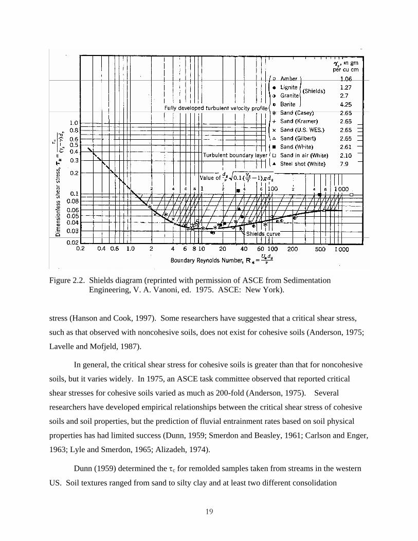
19
Figure 2.2. Shields diagram (reprinted with permission of ASCE from Sedimentation
Engineering, V. A. Vanoni, ed. 1975. ASCE: New York).
stress (Hanson and Cook, 1997). Some researchers have suggested that a critical shear stress,
such as that observed with noncohesive soils, does not exist for cohesive soils (Anderson, 1975;
Lavelle and Mofjeld, 1987).
In general, the critical shear stress for cohesive soils is greater than that for noncohesive
soils, but it varies widely. In 1975, an ASCE task committee observed that reported critical
shear stresses for cohesive soils varied as much as 200-fold (Anderson, 1975). Several
researchers have developed empirical relationships between the critical shear stress of cohesive
soils and soil properties, but the prediction of fluvial entrainment rates based on soil physical
properties has had limited success (Dunn, 1959; Smerdon and Beasley, 1961; Carlson and Enger,
1963; Lyle and Smerdon, 1965; Alizadeh, 1974).
Dunn (1959) determined the τc for remolded samples taken from streams in the western
US. Soil textures ranged from sand to silty clay and at least two different consolidation
20
pressures were used to mold each sample. The τc was determined using a submerged jet
impinging normally on the sample. Hydraulic shear stress was measured by placing a 1 in2 plate
at the location of the greatest soil scour. The following relationship was determined for soils
with a plasticity index of 5-16:
)73.130tan()180(001.0 PISvc ⋅+⋅+⋅=τ 2.3
where τc and the shear strength of the soil (Sv) are in psi, PI is the plasticity index in percent and
the argument of the tangent is in degrees. A rotating vane was used to determine Sv. Significant
correlation between τc and the silt+clay content of the soils was determined for those soils with a
high sand content. Increasing the fraction of fine particles in these coarser soils from 12.5% to
26% increased τc an order of magnitude.
Smerdon and Beasley (1961) tested 11 Missouri soils to determine the relationship
between τc and soil properties. The soil was loosely compacted in a flume and the hydraulic
shear stress was increased in increments until “general movement” of the bed was observed.
This point was defined as the critical tractive force. Soil properties, including Atterberg limits,
void ratio, aggregate analysis, specific gravity, particle size analysis and dispersion ratio, were
measured and compared to τc values using regression analysis. Significant simple linear
regression relationships were found between τc and the soil plasticity index (PI), dispersion ratio
(Dr), median grain size (D50), and percent clay. The critical tractive force increased with
increasing PI and percent clay, and decreasing Dr and D50.
Alizadeh (1974) developed a chart to predict the critical shear stress as a function of the
soil sodium adsorption ratio (SAR), the dielectric dispersion, and the pore water salt
concentration (TS), using artificial soil mixtures with distilled water as the eroding fluid (Figure
2.3). The SAR is defined as follows:
21
[ ][ ] [ ]
⎟⎟⎠
⎞⎜⎜⎝
⎛ +=
++
+
2
22 MgCa
NaSAR 2.4
where [Ca2+], [Mg2+] and [Na+] are the concentrations (meq/L) of calcium, and magnesium, and
sodium, respectively, in the soil pore water. This analysis does not consider the effects of soil
structure and aggregate stability on soil erosion (Thorne, 1982). Also, because distilled water
was used as the eroding fluid, these values represent the lower bound of critical shear stress for
soils.
Arulanandan et al. (1975) studied the effects of pore and eroding fluid on the erosion of a
Yolo Loam. The TS and SAR, as well as the eroding water salt concentration were varied. The
soil τc was determined using a rotating cylindrical apparatus, which consisted of two concentric
cylinders with 0.5 in annular space between. Soil samples were sieved and remolded into 7.6 cm
diameter, 8.1 cm long cylinders. The space between the soil sample and the outer cylinder was
filled with fluid and the outer cylinder was rotated to produce hydraulic shear on the sample.
The researchers determined the erosion rate increased with increasing SAR of the pore fluid,
while τc decreased (SAR of 1.4-154). Additionally, decreases in τc with increasing SAR were
more pronounced at low SAR; at higher SAR, τc changed little with increases in SAR. Increases
in TS resulted in increased τc, likely due to increased soil flocculation at high salt concentrations
(TS of 0.1, 0.01, and 0.005 N). The authors also evaluated the effects of SAR on the swelling of
soils at a TS of 0.005 N. Soil swelling increased with increases in SAR. Soil swelling has
significance for erosion because swelling increases the distance between soil layers and reduces
interparticle bonding, effectively reducing τc. Lastly, the effect of salt concentration in the
eroding fluid was investigated. The erosion rate increased and τc decreased with decreasing
NaCl concentrations in the eroding fluid, while little erosion occurred at NaCl concentrations
over 0.02 N. The increased erosion with decreasing eroding fluid salt concentration was
attributed to osmotic differences between the soil pore water and the eroding fluid. When the
salt concentration of the pore fluid is higher than that of the eroding fluid, water will move into
the soil, cause the soil to swell, and weaken interparticle forces. The magnitude of this depends
on how susceptible the soil is to swelling. When the electrolyte concentration of the eroding

22
.
fluid is greater than that of the pore water, water migrates out of the interlayer region and the soil
structure collapses, increasing soil stability.
Heinzen (1976) measured the soil erodibility and critical shear stress of 11 undisturbed
soil samples in a small flume, using distilled water as eroding fluid. Several methods of
predicting soil erodibility were compared. The TS, dielectric dispersion, SAR, organic matter
content, cation exchange capacity (CEC), Atterberg limits, dispersion ratio, texture, and density
of the test soils were measured. Free swell tests were also conducted. Heinzen noted that the
overall structure of the undisturbed samples played a significant role in their behavior during
erosion. The results indicated that erodibility methods that consider the chemical interaction
between the pore water and eroding fluid provide the best prediction of soil erodibility.
Arulanandan et al. (1980) conducted flume studies using undisturbed soil and stream
water samples from across the U.S. with the goal of developing a quantitative method to predict
the τc and the erosion rate of undisturbed natural soils. The results indicated that τc decreased
with increasing soil pore water SAR. Additionally, as the salt concentration of the eroding fluid
increased, the soil became more resistant to erosion. Figure 2.3 was developed to predict τc,
given the soil pore water SAR, the soil dielectric dispersion, and the salt concentration of the
eroding fluid. Once τc is known, the erosion rate can be estimated from Figure 2.4, which shows
the rate of change in the erosion rate at a given τc.
Osman and Thorne (1988) developed a model of bank toe erosion, based on the work of
Arulanandan et al. (1980). The critical shear stress for the bank material is determined from
Figure 2.3. If the stream shear stress is greater than τc, an initial rate of bank erosion (Ei) is
determined as:
)13.0(0223.0ceE ci
ττγ
−= 2.5
The actual soil erosion rate (E) is assumed to vary linearly with excess shear stress and is given
by the following:
)1( −=c
fiEE
ττ
2.6
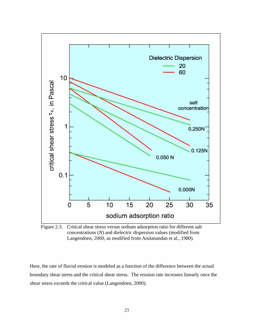
23
Figure 2.3. Critical shear stress versus sodium adsorption ratio for different salt concentrations (N) and dielectric dispersion values (modified from Langendoen, 2000, as modified from Arulanandan et al., 1980).
Here, the rate of fluvial erosion is modeled as a function of the difference between the actual
boundary shear stress and the critical shear stress. The erosion rate increases linearly once the
shear stress exceeds the critical value (Langendoen, 2000).
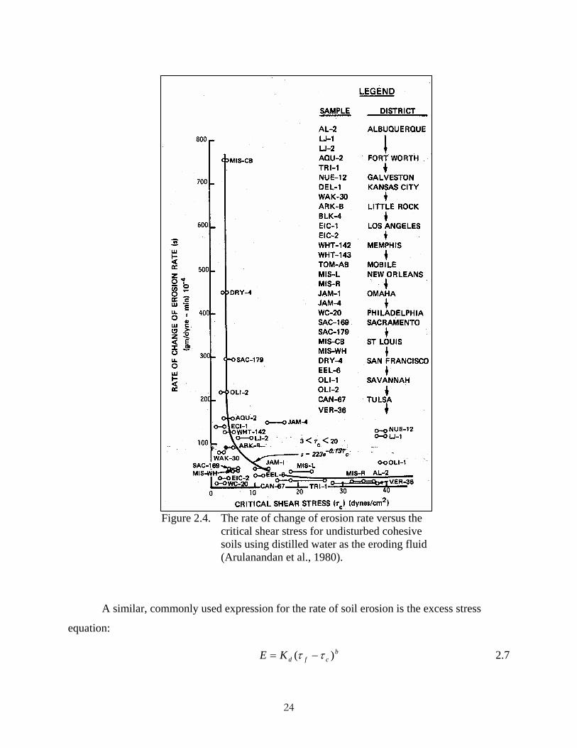
24
Figure 2.4. The rate of change of erosion rate versus the critical shear stress for undisturbed cohesive soils using distilled water as the eroding fluid (Arulanandan et al., 1980).
A similar, commonly used expression for the rate of soil erosion is the excess stress
equation:
bcfdKE )( ττ −= 2.7
25
where E is the erosion rate (cm3/hr/cm2); Kd is the erodibility coefficient (cm/hr/Pa); τ is the
actual shear stress (Pa); τc is the critical shear stress (Pa); and b is an exponent that is often
assumed to equal one (Hanson et al., 1999). Combining equations 2.5 and 2.6 and comparing
them to equation 2.7, it can be seen that Kd equals Ei/τc. The erosion resistance of the soil is
incorporated in both of the parameters, Kd and τc (Owoputi and Stolte, 1995). The excess stress
equation is used in several watershed models to calculate sediment erosion by fluvial
entrainment, including HEC-6, SWAT, and HSPF (USACE, 1993; Allen et al, 1997; Bicknell et
al., 1997). The excess stress equation is also used to model rill erosion in watershed models such
as WEPP. Research on rill erosion has shown b can vary between 1.0 and 1.5 (Van Klaveren
and McCool, 1998).
The erodibility coefficient can be considered a soil property that can be used to compare
relative erodibility and to classify soils for design purposes (Heinzen, 1976; Hanson, 1990a;
ASTM, 1999a). Various devices have been used to evaluate Kd in laboratory and field studies,
including pin hole erosion devices, straight and circular flumes, and rotating cylinders, disks and
impellers (Allen et al., 1997). Several researchers have used an impinging jet to study scour
because the initial flow pattern can be described by the jet size and velocity and that a
characteristic depth can be used to describe the scour (Rouse, 1940; Laursen, 1952; Dunn,
1959). Laursen (1952) proposed that the rate of scour beneath a jet will decrease with time as
the sour hole enlarges and will asymptotically approach zero as the decreasing hydraulic force
approaches the resistance of the soil.
Hanson (1989; 1990a; 1990b; 1991) developed an in situ testing procedure to determine
Kd and τc of channel beds using a submerged, vertical jet device. Several studies have used
submerged jets for determining soil critical shear stress (Dunn, 1959; Moore and Masch, 1962;
Hollick, 1976). A similar device for testing bank material has been developed in cooperation
with the USDA Sedimentation Laboratory in Oxford, MS (Hanson, 2001). Hanson and Cook
(1997) adapted analytical procedures developed by Stein et al. (1993) and Stein and Nett (1997)
for a planar overfall jet to determine Kd and τc for scour created by a submerged jet. Figure 2.5
shows a diagram of the submerged jet testing device. A circular jet at a uniform velocity, Uo, is
produced by a nozzle of diameter do, under pressure h, and hits the soil bed at right angles. The
jet velocity is calculated as follows:
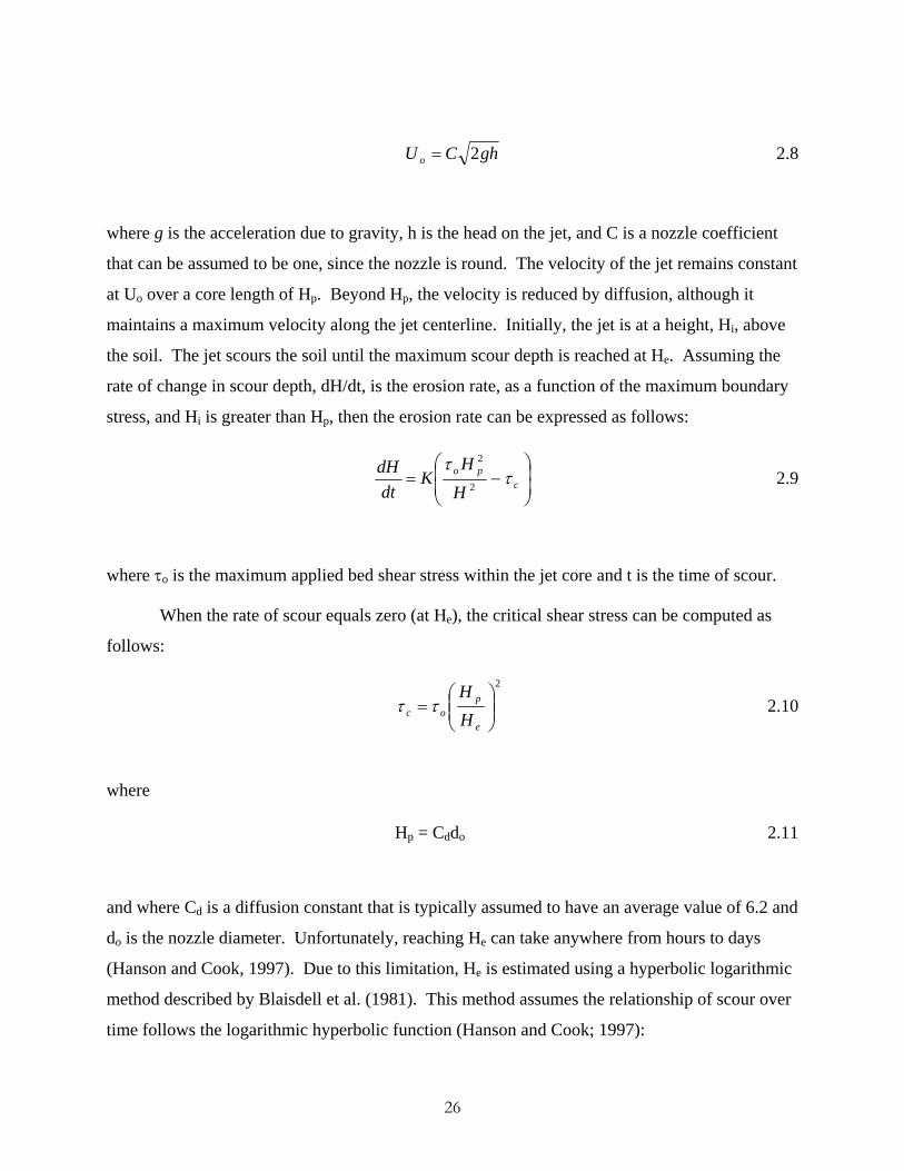
26
ghCU o 2= 2.8
where g is the acceleration due to gravity, h is the head on the jet, and C is a nozzle coefficient
that can be assumed to be one, since the nozzle is round. The velocity of the jet remains constant
at Uo over a core length of Hp. Beyond Hp, the velocity is reduced by diffusion, although it
maintains a maximum velocity along the jet centerline. Initially, the jet is at a height, Hi, above
the soil. The jet scours the soil until the maximum scour depth is reached at He. Assuming the
rate of change in scour depth, dH/dt, is the erosion rate, as a function of the maximum boundary
stress, and Hi is greater than Hp, then the erosion rate can be expressed as follows:
⎟⎟⎠
⎞⎜⎜⎝
⎛−= c
po
HH
Kdt
dH ττ
2
2
2.9
where τo is the maximum applied bed shear stress within the jet core and t is the time of scour.
When the rate of scour equals zero (at He), the critical shear stress can be computed as
follows:
2
⎟⎟⎠
⎞⎜⎜⎝
⎛=
e
poc H
Hττ 2.10
where
Hp = Cddo 2.11
and where Cd is a diffusion constant that is typically assumed to have an average value of 6.2 and
do is the nozzle diameter. Unfortunately, reaching He can take anywhere from hours to days
(Hanson and Cook, 1997). Due to this limitation, He is estimated using a hyperbolic logarithmic
method described by Blaisdell et al. (1981). This method assumes the relationship of scour over
time follows the logarithmic hyperbolic function (Hanson and Cook; 1997):
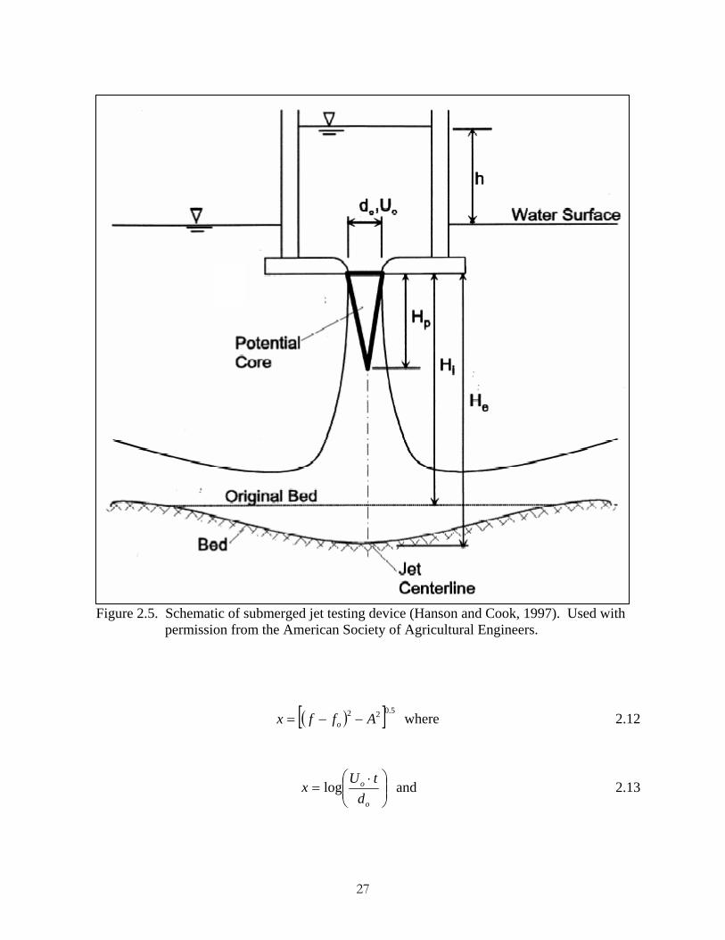
27
Figure 2.5. Schematic of submerged jet testing device (Hanson and Cook, 1997). Used with permission from the American Society of Agricultural Engineers.
( )[ ] 5.022 Affx o −−= where 2.12
⎟⎟⎠
⎞⎜⎜⎝
⎛ ⋅=
o
o
dtUx log and 2.13
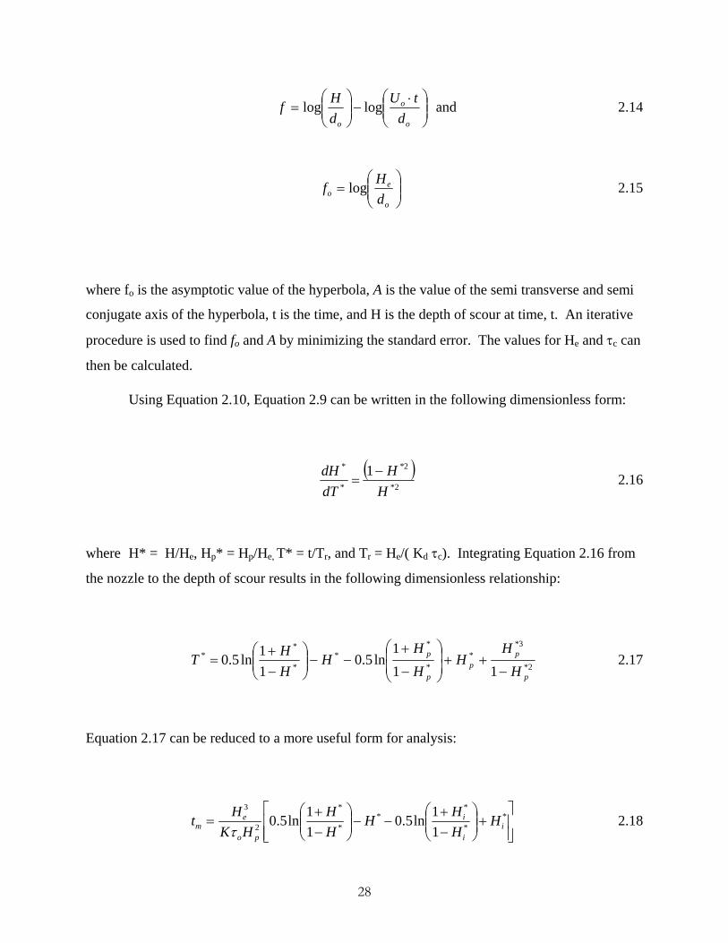
28
⎟⎟⎠
⎞⎜⎜⎝
⎛ ⋅−⎟⎟
⎠
⎞⎜⎜⎝
⎛=
o
o
o dtU
dHf loglog and 2.14
⎟⎟⎠
⎞⎜⎜⎝
⎛=
o
eo d
Hf log 2.15
where fo is the asymptotic value of the hyperbola, A is the value of the semi transverse and semi
conjugate axis of the hyperbola, t is the time, and H is the depth of scour at time, t. An iterative
procedure is used to find fo and A by minimizing the standard error. The values for He and τc can
then be calculated.
Using Equation 2.10, Equation 2.9 can be written in the following dimensionless form:
( )2*
2*
*
* 1H
HdTdH −
= 2.16
where H* = H/He, Hp* = Hp/He, T* = t/Tr, and Tr = He/( Kd τc). Integrating Equation 2.16 from
the nozzle to the depth of scour results in the following dimensionless relationship:
2*
3**
*
**
*
**
111
ln5.011ln5.0
p
pp
p
p
HH
HHH
HHHT
−++⎟
⎟⎠
⎞⎜⎜⎝
⎛
−
+−−⎟⎟
⎠
⎞⎜⎜⎝
⎛−+
= 2.17
Equation 2.17 can be reduced to a more useful form for analysis:
⎥⎥⎦
⎤
⎢⎢⎣
⎡+⎟⎟
⎠
⎞⎜⎜⎝
⎛−+
−−⎟⎟⎠
⎞⎜⎜⎝
⎛−+
= **
**
*
*
2
3
11ln5.0
11ln5.0 i
i
i
po
em H
HHH
HH
HKHtτ
2.18
29
where tm is the measured time from the start of the jet test. The two unknowns, He and Kd, need
to be fitted, such that the predicted tm most closely matches the actual tm. The estimate of He is
used to narrow the possible combinations of He and Kd, and a least-squares regression of the
predicted tm versus the actual tm is used to obtain the best fit estimates of He and Kd. The critical
shear stress is computed from Equation 2.10. These analytical procedures have been coded in an
Excel spreadsheet by Hanson and Cook, as modified by the author for data input in SI units.
Figure 2.6 shows a plot of H* versus T* with the best fit line from site ST2.
Allen et al. (1997) used Hanson’s jet test device to develop predictive equations of soil
erodibility in Texas for use in the SWAT model. They used data from 30 streams and stratified
the soils based on the percentage of clay and the soil activity. Soils were tested for bulk density,
void ratio, Atterberg limits, and soil texture. A highly significant regression was obtained for
each of the three soil categories (r2 = 0.78-0.96). For soils with less than 10% clay, the
antecedent moisture content and the percentage of sand were the most important predictors of
soil erodibility. The second category contained soils with >10% clay and activities <1.25. Bulk
density, percent clay, and plastic limits were the best indicators of erodibility for these soils. The
most cohesive soils were in the third category, where clay contents and soil activities were higher
than 10% and 1.25, respectively. For these soils, the complete soil textural classification and the
liquid limit produced the best prediction of soil erosion potential. Additionally, the authors noted
that the presence and density of roots seemed to influence soil erodibility, although this
parameter was not quantified. The authors demonstrated an application of the data in a SWAT
model to evaluate the effects of urbanization and climate change on long term channel
degradation.
2.3. Mass Wasting
Mass wasting occurs when the weight of the bank is greater than the shear strength of the
soil (Osman and Thorne, 1988). It often results from increases in bank height or bank angle due
to fluvial erosion and the presence of tension cracks (ASCE, 1998a; Simon et al., 2000). Mass
wasting depends on bank geometry and stratigraphy, properties of the bank materials, and the
type and density of bank vegetation (Thorne, 1990; Abernethy and Rutherfurd, 1998).
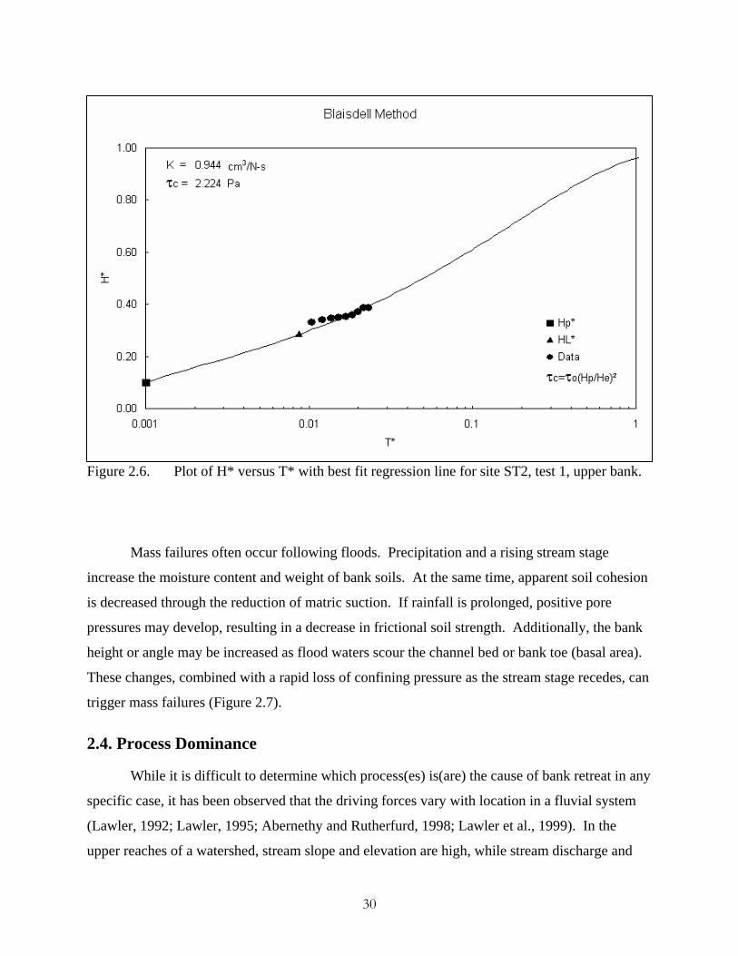
30
Figure 2.6. Plot of H* versus T* with best fit regression line for site ST2, test 1, upper bank.
Mass failures often occur following floods. Precipitation and a rising stream stage
increase the moisture content and weight of bank soils. At the same time, apparent soil cohesion
is decreased through the reduction of matric suction. If rainfall is prolonged, positive pore
pressures may develop, resulting in a decrease in frictional soil strength. Additionally, the bank
height or angle may be increased as flood waters scour the channel bed or bank toe (basal area).
These changes, combined with a rapid loss of confining pressure as the stream stage recedes, can
trigger mass failures (Figure 2.7).
2.4. Process Dominance
While it is difficult to determine which process(es) is(are) the cause of bank retreat in any
specific case, it has been observed that the driving forces vary with location in a fluvial system
(Lawler, 1992; Lawler, 1995; Abernethy and Rutherfurd, 1998; Lawler et al., 1999). In the
upper reaches of a watershed, stream slope and elevation are high, while stream discharge and
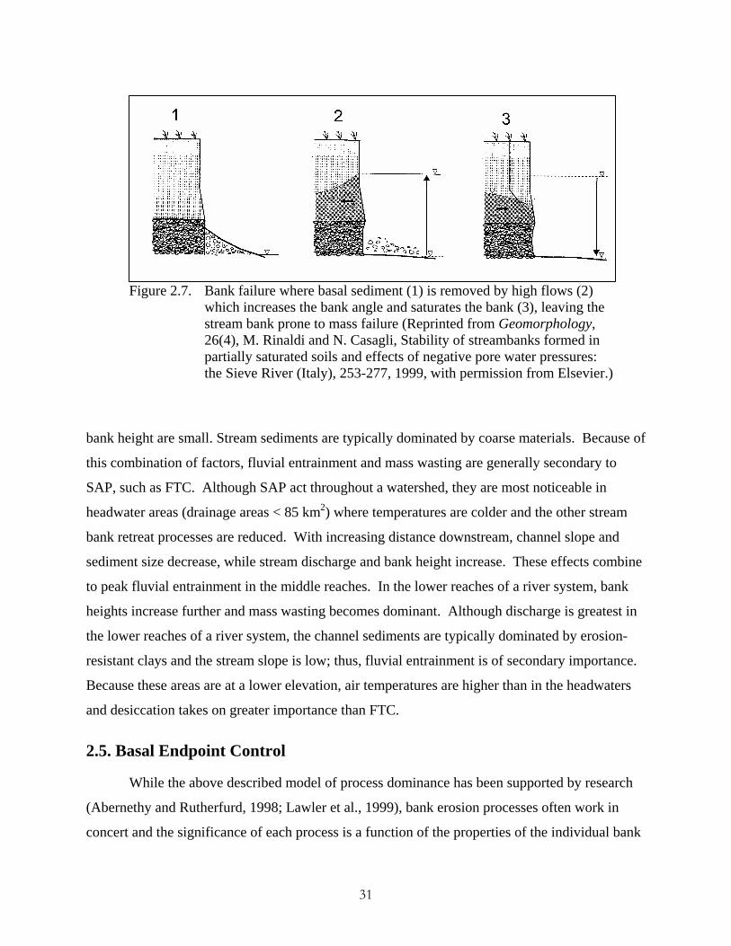
31
Figure 2.7. Bank failure where basal sediment (1) is removed by high flows (2) which increases the bank angle and saturates the bank (3), leaving the stream bank prone to mass failure (Reprinted from Geomorphology, 26(4), M. Rinaldi and N. Casagli, Stability of streambanks formed in partially saturated soils and effects of negative pore water pressures: the Sieve River (Italy), 253-277, 1999, with permission from Elsevier.)
bank height are small. Stream sediments are typically dominated by coarse materials. Because of
this combination of factors, fluvial entrainment and mass wasting are generally secondary to
SAP, such as FTC. Although SAP act throughout a watershed, they are most noticeable in
headwater areas (drainage areas < 85 km2) where temperatures are colder and the other stream
bank retreat processes are reduced. With increasing distance downstream, channel slope and
sediment size decrease, while stream discharge and bank height increase. These effects combine
to peak fluvial entrainment in the middle reaches. In the lower reaches of a river system, bank
heights increase further and mass wasting becomes dominant. Although discharge is greatest in
the lower reaches of a river system, the channel sediments are typically dominated by erosion-
resistant clays and the stream slope is low; thus, fluvial entrainment is of secondary importance.
Because these areas are at a lower elevation, air temperatures are higher than in the headwaters
and desiccation takes on greater importance than FTC.
2.5. Basal Endpoint Control
While the above described model of process dominance has been supported by research
(Abernethy and Rutherfurd, 1998; Lawler et al., 1999), bank erosion processes often work in
concert and the significance of each process is a function of the properties of the individual bank
32
system (Grissinger, 1982). Bank erosion mechanisms are linked in a process termed basal
endpoint control where the balance between the rate of bank material delivery to the basal area
and the subsequent removal rate of that material by the stream determine the ultimate rate of
bank retreat (Thorne, 1990). Initially, fluvial erosion removes material from the stream basal
area, increasing bank height and/or angle. This removal causes mass instability and failure of the
bank. The failed material is delivered to the toe of the bank; it may be immediately entrained or
it may remain at the toe until subsequent high flows remove it. If the material is not removed, it
will reinforce the bank and reduce further mass failures. Three states of basal endpoint control
are defined as follows (Thorne, 1982):
1. Impeded removal - The supply of failed material exceeds the ability of the stream to
remove it. The failed material serves to stabilize the bank, reducing the supply of
eroded soil.
2. Unimpeded removal - The supply and removal rates are equal, such that the bank
height and angle remain constant. The rate of parallel bank retreat is controlled by
the stream flow.
3. Excess basal capacity - The material removal rate exceeds the supply from the banks.
This high removal rate leads to scour of the basal area, increasing the bank height and
angle and decreasing bank stability. This instability increases the supply of material
to the stream and moves the system toward a state of unimpeded removal.
2.6. Effects of Vegetation on Stream Bank Stability
Little specific information is available on the effects of vegetation on stream bank
stability (Abernethy and Rutherfurd, 1998). It is generally established that vegetation influences
the chemical and physical properties of stream banks, as well as the local microclimate. The
following sections describe the effects of vegetation on the three processes implicated in stream
bank retreat. Also, the impacts of woody versus herbaceous plants are compared.
2.6.1. Subaerial Processes
Riparian vegetation has multiple effects on SAP (Wu, 1984; Abernethy and Rutherfurd,
1998). A dense cover of vegetation absorbs the energy of rainfall, reducing soil detachment by
raindrop impact (Gray and Leiser, 1982; Coppin and Richards, 1990). Sheet and rill erosion are
33
decreased several orders of magnitude due to interception storage, improved infiltration,
increased flow resistance, and the stabilizing influence of roots on surface soils (Thorne, 1982;
Gurnell and Gregory, 1984; Thorne, 1990). Alternatively, roots may increase the susceptibility
of a bank to fluvial erosion by loosening the bank soil (Thorne, 1990).
Vegetation insulates the stream bank from extreme temperature fluctuations (Abernethy
and Rutherfurd, 1998). This insulation minimizes the occurrence of freezing and cracking due to
desiccation (Thorne, 1990). Amarasinghe (1992) found a decrease in evaporation improved soil
moisture retention in vegetated banks, as compared to bare banks, reducing the risk of
desiccation and slaking. However, Davidson et al. (1991) noted that in dry years, clay stream
bank soils under vegetation with high evapotranspiration rates (grass and early successional
trees) dried to near the wilting point and developed extensive fissures that lasted for several
years. These cracks did not occur under more advanced successional trees which had an
extensive litter layer and lower evapotranspiration rates.
The effects of vegetation on winter stream bank soil temperatures were studied in
northeastern Nevada (Bohn, 1989). Soil temperature was measured at a depth of 3 cm in four
sets of paired bare and vegetated stream banks. Bank vegetation consisted of Kentucky
bluegrass and sparse willows. Soil temperatures were recorded every 3 hours from January
through May 1987 and average daily soil maximum and minimum temperatures, and daily
temperature range were calculated for days when snow cover was absent. Results were analyzed
using paired t-tests and showed that the bare stream banks underwent twice the number of FTCs
as the vegetated banks. Furthermore, the grass banks had a significantly higher daily minimum
temperature and a significantly lower daily maximum temperature, resulting in a lower overall
daily temperature range. In addition to reducing near surface wind velocities and insulating
against nighttime radiative cooling, vegetation reduces soil bulk densities. The presence of roots
and increases in organic matter content result in greater numbers of air-filled pores, which lowers
heat conductivity through the soil (Bohn, 1989).
Stott (1997) measured stream bank retreat rates on two streams in central Scotland. One
of the streams was dominated by a Sitka spruce plantation, while the riparian area of the second
stream contained primarily moorland vegetation, such as grasses, bracken, and heather. Bank
retreat rates were measured using erosion pins. Minimum and maximum daily air temperatures
34
on the stream banks were also recorded on 13 occasions during the six month study period.
Bank retreat rates were greatest in the winter on both streams, but the moorland stream had a
generally higher retreat rate than the forested stream. The authors attributed this finding to a
decreased incidence of frost along the forested stream: air temperatures under the spruce
plantation averaged 3.7oC higher than under the moorland vegetation and bank retreat was
correlated to the incidence of frost.
2.6.2. Fluvial Entrainment
The influence of vegetation on stream hydraulics has long been recognized (Zimmerman
et al., 1967; Hickin, 1984). Vegetation provides increased channel roughness, directing flows
towards the center of the channel and reducing flow velocities and shear stresses along the banks
(Beschta and Platts, 1986; Gregory and Gurnell, 1988; McKenney et al. 1995; Thorne and
Furbish, 1995; Hupp, 1999; Simon and Darby, 1999; Tsujimoto, 1999). Since sediment transport
capacity is proportional to flow velocity to the sixth power (v6), small decreases in stream
velocity can result in large changes in sediment transport (Thorne, 1990). Additionally,
vegetation damps near bank turbulence and weakens secondary currents in river bends, further
reducing fluvial entrainment (Thorne and Furbish, 1995; Abernethy and Rutherfurd, 1998). It
should be recognized that the effects of vegetation on stream hydraulics varies with season,
stream stage, and stream width to depth ratio, particularly for herbaceous species (Gregory and
Gurnell, 1988; Thorne and Osman, 1988; Masterman and Thorne, 1992; Abernethy and
Rutherfurd, 2000). Additionally, the spacing of vegetation along a stream is a crucial
determinant of the distribution of hydraulic stresses (Pizzuto and Mecklenburg, 1989; Thorne et
al., 1997).
Vegetation has multiple effects on the distribution of energy and sediment in a stream.
Along streams with forested riparian buffers, fallen trees create series of step pools, dissipating
stream energy and providing sediment storage (Beschta and Platts, 1986). Hupp (1999) noted
that roots growing under stream channels may provide grade control to limit headcut migration.
Additionally, vegetation can act as a nucleus for the creation of sediment bars; vegetation is
effective in trapping washload (Hickin, 1984; Thorne, 1990; McKenney et al. 1995; Hupp,
1999). These benefits may be offset by the fact that the presence of downed trees and isolated
stands of vegetation can produce locally severe scour of the stream bed and banks, although the
35
magnitude of this effect depends on the size of the stream or river (Thorne, 1990; McKenney et
al. 1995).
2.6.2.1. Effects of Root Density on Soil Erodibility
While considerable research has been conducted on fluvial entrainment, little quantitative
information is available on the effects of vegetation on soil scour by concentrated flow (Smith,
1976; Kamyab, 1991; Dunaway et al., 1994; Mamo and Bubenzer, 2001a). It is believed the root
systems of woody and herbaceous plants physically bind bank soils in place, increasing τc (Gray
and Leiser, 1982; Coppin and Richards, 1990; Thorne et al., 1997). Additionally, roots exudates
may increase soil cohesion chemically (Amarasinghe, 1992; Thorne et al., 1997). Odgaard
(1987) studied erosion along meander bends of two major rivers in Iowa and determined that
erosion along wooded stream banks was half that along sparsely vegetated banks.
Smith (1976) measured stream bank erosion rates in Banff Park, Alberta using bank pins
and an instream erosion box. These rates were compared to root volume ratios (RVRs, root
volume per unit soil volume) under riparian meadow and scrub willow vegetation in silty soils.
Root volume ratios ranged from 10% to 21% and the log of the erosion rate decreased linearly
with increases in the percentage of root volume. Due to the cold climate, a dense root mat
formed on the bank face to depths of 3.5 m and effectively armored the stream bank. This root
mat reduced the erosion rate by a factor of 20,000, as compared to bare soil.
Kamyab (1991) measured soil erodibility using soil core samples from three meadow
plant communities in the Sierra Nevada Mountains in California. Samples from depth
increments of 1-10 cm and 30-40 cm were tested in a laboratory flume under hydraulic stresses
of 0.59, 6.2, and 15.7 Pa. The soils were tested for root length density (RLD) and dry root
biomass, as well as void ratio, organic carbon, clay content and activity, mean particle size and
standard deviation, dispersion ratio, and plasticity index. Root length density is the length of
roots in a unit soil volume. Using regression analysis, Kamyab determined erosion resistance
was directly proportional to total, fine, and rhizome root length density, as well as total dry root
biomass. Erosion was minimal at root length densities in excess of 300 cm/cm3. At lower
RLDs, soil properties, such as clay content, mean grain size, dispersion ratio, and plasticity index
influenced soil erosion.
36
In a follow-up study similar to Kamyab (1991), Dunaway et al. (1994) assessed the
interaction between soil and plant characteristics and their impact on erosion rates for riparian
meadow communities in the Sierra Nevada Mountains. Samples from the banks of five streams
were tested in a flume and the effects of root density, soil texture, and plant community were
assessed with multivariate analysis. Average RVR ranged from 0.0027 to 0.0063. Erosion rates
were inversely related to RVR and percent silt, but directly proportional to clay content. This is
contrary to previous research which showed increasing erosion resistance with increases in clay
content (Grissinger et al., 1981). The authors attributed this discrepancy to the low root density
of high clay content soils.
Mamo and Bubenzer (2001a) conducted laboratory experiments on the effects of live
ryegrass roots on soil detachment, erodibility, and critical shear stress. Soil cores with 100 mm
diameters were filled with sieved Plano silt loam and planted at two different densities. The
samples were then grown in a greenhouse for periods of six to sixteen weeks. Fallow and rooted
soil cores were eroded in a flume using five flow rates of 7.57-37.85 L/min at depths of 3.96-
8.23 mm. In addition to measuring erosion rates, soil shear strength, organic matter content,
aggregate stability, and root length density were assessed. Results showed that soil strength
increased with time for both rooted and fallow soils, but the increase in strength was more
significant for the rooted soils. Both soil detachment rate (Dr) and erodibility (Kd) decreased
with time and root density. Detachment rates for rooted versus fallow samples decreased 35-
73% while erodibility rates were reduced 8-87%. Reductions in both Dr and Kd for both the
fallow and planted samples were attributed to increases in interparticle forces with increasing
time and successive WDCs. In contrast to soil detachment and erodibility, there were no
significant differences in τc between rooted and fallow soils and no changes over time were
noted. Additionally, there was no apparent relationship between Kd and τc, as indicated by
previous research (Foster, 1982). The researchers reported an inverse exponential relationship
between Dr and root length density, with exponents ranging from -0.02 to -0.50 and correlation
coefficients ranging from 0.22 to 0.83. Increases in both aggregate stability and organic carbon
content were noted for the rooted samples, while those properties remained constant in the fallow
cores.
37
Mamo and Bubenzer (2001b) extended their study of the effects of live roots on rill
erodibility in a field plot study using corn and soybeans. Semicircular rills, 5.3 m long and 63.5
mm deep were constructed in freshly tilled, fallow, corn, and soybean plots. Rill cross section
and wetted area were measured over time with an imaging device and a pin profiler for five
different flow rates, ranging from 7.57-37.85 L/min, at three different crop stages. Erosion rates,
soil strength, root length density, soil aggregate stability, and carbon content were also measured.
Soil erodibility and critical shear stress (Kd and τc) were determined by plotting the erosion rate
versus the applied shear stress. Soil strength was over 20% greater under corn and soybeans than
under fallow conditions. As with the laboratory study, the soil detachment rate was influenced
by RLD, the stage of plant growth, and time. On average, Dr for corn and soybeans was 50%
less than the Dr for fallow conditions. The authors showed that Dr decreased exponentially with
increasing RLD. The exponents varied from -0.09 for corn to -2.3 for soybean, with r2 of 0.14 -
0.54. This decrease in Dr with increasing RLD was attributed to the physical restraint of soil
particles by roots. The presence of corn and soybeans roots also decreased Kd over 50%. As
with the laboratory study, there was no correlation between τc and either K or Dr; τc decreased
with both time and growth stage. This decrease in τc was attributed to small variations in
detachment rates at low flows. While both aggregate stability and soil organic carbon content
decreased under fallow conditions, both increased with increasing RLD, indicating the influence
of roots on soil physical properties.
2.6.2.2. Effects of Roots on Soil Properties
Vegetation indirectly affects soil erosion by changing soil physical and chemical
properties including soil organic matter, aggregate stability and bulk density (Mamo and
Bubenzer, 2001a,b). While the effects of vegetation on soil structure is well known, the impacts
have not been well quantified (Materechera et al., 1992). Reid and Goss (1980) evaluated the
effects of ryegrass on the aggregate stability of a sandy loam. Ryegrass was grown in pots for
four weeks and the aggregate stability of the planted pots was compared to fallow pots using
turbidimetric analyses and wet sieving. Most of the roots were removed prior to testing by
sieving the soil through a 4.0 mm mesh. Results showed that after only four weeks the ryegrass
significantly increased aggregate stability, predominately for the larger aggregates. The authors
attributed this increase in soil stability to root exudates. Since the pots were maintained at a
38
constant moisture content, soil consolidation due to WDC did not occur. Additionally, the
researchers observed soil particles attached to plant mucilage around the root tips.
In a follow-up study, Reid and Goss (1981) investigated the effects of lucerne, maize,
perennial ryegrass, tomato and wheat on the aggregate stability of both “fresh” and air-dried
samples from two soils. A sandy loam and silt loam were sieved through a 2.0 mm mesh and
placed in pots at a constant moisture content. The plant were only grown for periods of either 25
or 42 days, depending on growth rate, to minimize the effects of increases in organic matter from
root decomposition on aggregate stability. Soils were maintained at a constant water content
throughout the study. Using turbidimetric analyses and wet sieving, the aggregate stability of
both fresh and rapidly air-dried soils were measured. Additionally, root length and weight, root
hair length, and the degree of infection by mycorrhizal fungi were assessed. The results
indicated the growth and activity of ryegrass and lucerne roots significantly increased aggregate
stability. Increases in soil stability were attributed to polysacharide mucilages produced in the
plant rhizospheres. No correlation between aggregate stability and root length or root hair length
was shown. In contrast to the lucerne and ryegrass, the stability of fresh aggregates decreased
under maize, tomato and wheat, although results were not conclusive for tomato or wheat. In
contrast, the stability of air-dried aggregates under wheat was greater than the fallow controls.
The authors suggest difference in aggregate stability resulted from variations in the
polysaccharides produced by the five plant species.
Materechera et al. (1992) evaluated the effects of plants and WDC on aggregate
formation in two agricultural soils in Australia. A loam and a hydromorphic clay were air-dried,
ground, and sieved through a 0.5 mm mesh to destroy the existing macrostructure. Soil
"minirhizotrons" were created and planted with pea, wheat and ryegrass. Unplanted
minirhizotrons were used as controls. Designed as a 2x4x2 factorial experiment, half of the pots
underwent 15 WDCs while the other half were maintained at constant moisture levels. The
samples were maintained for four to seven months, depending on the length of time required to
undergo 15 WDCs. Aggregate size distribution, aggregate stability (wet-sieving of air-dry
samples), aggregate tensile strength, root length density, aggregate bulk density, and aggregate
organic carbon contents were measured. Results of the study showed that RLD increased in the
order of ryegrass>wheat>pea and that RLD was positively correlated to aggregate size
distribution, stability, tensile strength, bulk density and organic carbon content. The effect of
39
plants on aggregate formation was attributed to increases in soil stress during root penetration, as
well as chemical stabilization by the production of mucilage and the establishment of soil
microorganisms. Multiple WDCs also produced significant aggregate formation through
increases in soil tensile stress and soil cracking. While both plants and WDC were significant in
the formation of soil aggregates, the authors felt changes in water regime were more important
for aggregate formation than plants.
Haynes and Beare (1997) studied the effects of barley, wheat, prairie grass, Italian
ryegrass, and two legumes, white clover and lupin, on soil organic matter and aggregate stability
in a silt loam soil. Root mass and length, microbial biomass carbon, soil organic carbon, total
and extractable soil carbohydrate content, bacterial number and fungal hyphae length were also
measured. The six plant species were grown in pots for 12 weeks before sampling. The results
showed that plants have a significant effect on aggregate stability and microbial biomass carbon,
with microbial biomass and aggregate stability increasing with root length and root mass. Roots
and fungal hyphae increase aggregate stability by creating a physical mesh that binds soil
particles and by exuding polysaccharides and other organic substrates which act as soil glues.
Additionally, increases in total root mass increase soil organic carbon, which in turn leads to an
increase in soil microbes. Similar to plants, soil microbes influence soil stability by exuding
polysaccharide and phenolic binding agents.
2.6.2.3. Root Density in Stream Banks
The influence of root density and vegetation type on the erosion of red clay soils in the
western Lake Superior basin was investigated by Davidson et al. (1991). Root biomass was
determined by excavating 0.5 m2 quadrats in 10 cm increments to a depth of 0.5 m. Roots were
separated into 10 diameter classes. In general, root mass in clay soil under forested vegetation
had twice the root biomass as under herbaceous vegetation. Root distribution with depth was
dependant on soil type: in clay soils most of the root biomass was found in the top 50 cm of the
soil profile, while in sandy soils the roots extended to greater depths. Vegetation type also
influenced root distribution. In clay soils, 90% of the herbaceous root mass was located in the
upper 10 cm, as compared to 50% for woody vegetation.
Shields and Gray (1992) studied sand levees on the Sacramento River, California. Five
sites with woody vegetation were compared to a herbaceous control. Root distributions were
40
measured for seven diameter classes using the profile wall method (Bohm, 1979). Root density
decreased exponentially with root diameter. Average root area ratios (RARs) ranged from
0.001% to 2.02%, with an average of 0.17%. Root area ratio is the total root area per unit area of
soil on a profile wall. The largest RAR was observed in the top 10 cm of the herbaceous control,
although this was biased by the presence of a single large root. On average, 43% and 50% of the
woody and herbaceous root area, respectively, occurred in the top 30 cm of the soil profile. At
depths greater than 20 cm, there were no significant differences in RAR under woody and
herbaceous vegetation. Herbaceous roots were short and oriented vertically. In contrast, woody
roots radiated from laterally from the root crown, parallel to the ground surface. The authors
noted that the woody roots generally angled downward and attributed this orientation to the
droughty sandy soils.
The root distribution for two species of Australian riparian trees was investigated by
Abernethy and Rutherfurd (2001). Root area ratio was measured along profile walls at varying
distances from the tree thickets and at depths of 1 – 2 m. The RARs ranged from 0.001% to
0.756% and generally decreased with depth and distance from the trees. Some scatter occurred
in the measurements made near the trees: RAR is biased by the presence of individual large
roots.
Simon and Collison (2002) measured RAR for four common riparian tree species and
two grass species in the Goodwin Creek Experimental Watershed in northern Mississippi. The
trees ranged in age from 5 years to 12 years, while the grasses were 5 years old. Average RARs
varied from 0.0056% to 0.012% for the trees and from 0.0044% to 0.014% for the grasses.
While the RARs were similar for the trees and grasses, the number of roots per unit area was one
to two orders of magnitude greater for the grasses than for the trees. The majority of the roots
were small diameter: the tree roots were generally less than 2 mm in diameter and the grass
roots were mostly smaller than 1 mm. The largest tree root diameters were 9 – 16 mm, while the
largest grass roots were less than 3 mm in diameter. Roots were concentrated in the upper soil
profile with 90% of the roots in the top 17 cm for eastern gamma grass (Tripsicum dactyloides),
32 cm for black willow (Salix nigra), 38 cm for sweetgum (Liquidambar styroflora), 56 cm for
switch grass (Panicum virgatum ‘Alamo’), and 74 cm for sycamore (Platanus occidnetalis). The
roots were generally oriented horizontally, except the switch grass roots, which were oriented
vertically.
41
2.6.3. Mass Wasting
Researchers have found that woody and herbaceous roots significantly increased slope
stability over bare conditions (Waldron and Dakessian, 1982; Gray and MacDonald, 1989;
Shields and Gray, 1992). The root systems of woody and herbaceous plants act to stabilize
banks by increasing soil shear strength (Wu and McKinnell, 1976; Murgatroyd and Ternan,
1983; Abernethy and Rutherfurd, 2001). Soils are strong in compression, but weak in tension;
shear stress in the soil is transferred to tensile stress in the roots (Thorne, 1990; Langendoen,
2000). Even small increases in root density can substantially increase soil strength (Gray and
MacDonald, 1989; Abernethy and Rutherfurd, 2001). Micheli and Kirchner (2002) measured a
linear relationship between riparian meadow root biomass and soil shear strength, with riparian
vegetation increasing soil shear strength as much as 800%.
Changes in soil strength are a function of root size, distribution, and tensile strength
(Abernethy and Rutherfurd, 2001). Several researchers have found a nonlinear inverse
relationship between root strength and root diameter (Waldron and Dakessian, 1981; Abernethy
and Rutherfurd, 2001; Simon and Collison, 2001). Large roots (> 15– 20 cm in diameter) do
little to increase shear strength, but instead act as soil anchors (Simon and Darby, 1999).
Additionally, the stems of woody plants act as soil buttresses and arches, further protecting banks
against mass failure (Abernethy and Rutherfurd, 1998). In a study of two different tree species,
Abernethy and Rutherfurd (2001) determined root strength was unrelated to species or test
method. Roots typically fail by tensile or bond failure, although scour of exposed roots also
occurs (Wu, 1984; Thorne, 1990; Abernethy and Rutherfurd, 2001). The ability of roots to resist
pullout is a function of root length, branching patterns, root tortuosity, and soil type (Abernethy
and Rutherfurd, 2001).
Tengbeh (1993) studied the effect of perennial ryegrass roots (Lolium perenne) and soil
moisture content (MC) on soil shear strength. Both a sandy clay loam and a clay were dried and
sieved in 2 mm sieve. The soils were planted at different densities (100, 190, 380 seeds/m2) and
grown in a greenhouse for different periods of 4 - 30 weeks. Soil shear strength was measured
with a hand-held direct vane shear tester, while root density was quantified by sampling root
biomass. The results of the study showed that soil shear strength of both rooted and unrooted
samples increased exponentially as the soils dried. The rate of change in shear strength with MC
was greatest for rooted soils at low moisture contents. Roots increased shear strength by at least
42
500% for the sandy clay loam and up to 850% for clay at MC near saturation. Additionally, the
rooted soils attained a maximum shear strength at a lower MC than root-free soils. The authors
attributed these findings to root exudates, suggesting that the root exudates helped bind the soils.
The MC of maximum strength for the rooted soils was well below the soil plastic limit;
therefore, the concept that the maximum shear strength occurs at the soil plastic limit may not
apply to rooted soils. Because the amount of reinforcement provided by the roots varied with
soil texture, the authors questioned the accuracy of bank stability models that assume increases
in soil cohesion due to roots are a function of root density only.
2.6.4. Benefits of Herbaceous vs. Woody Vegetation
As discussed in the Introduction section, there is considerable debate in the literature
regarding the relative merits of herbaceous versus woody riparian vegetation (Lyons et al., 2000;
Simon and Collison, 2001). With regard to subaerial processes, Stott (1997) found that soil
temperature and moisture regimes were moderated by forest cover, as compared to moorland
vegetation. Soil temperature in the forest was an average of 3.7ºC higher. As a result, stream
banks with forested riparian buffers may experience fewer WDCs or FTCs.
Both herbaceous and woody vegetation provide increased hydraulic roughness, although
the effects of herbaceous vegetation are reduced at high flows because grasses and forbs bend
over in the flow. Additionally, herbaceous vegetation is absent or reduced during the winter
when most channel erosion occurs. As a result of reduced stream width, velocities in grass
channels have been found to be greater than those with forested vegetation (Horwitz et al., 2000)
In addition to hydraulic effects, vegetation type appears to influence stream sediment
regime. Bedload transport rates under forested buffers are 2 - 6 times those measured under
herbaceous buffers (Murgatroyd and Ternan, 1983; Stott et al., 1986; Kirby et al., 1991; Reed,
1999). Reed (1999) attributed this difference to a greater water surface slope in forested sections
and increased sediment storage in grassed reaches.
Herbaceous vegetation has a greater density of fine roots, as compared to woody
vegetation (Tufekcioglu et al., 1999). This high root density will likely produce greater τc and
shear strength under herbaceous vegetation. Several authors claim stream channels are narrower
with grass buffers because the grass acts to armor stream banks and trap fine sediments
(Murgatroyd and Ternan, 1983; Sweeney, 1993; Trimble, 1997b; Davies-Colley, 2000; Lyons et
43
al., 2000; Simon and Collison, 2001); however, bank reinforcement extends only to the rooting
depth (Thorne, 1990). While trees have fewer fine roots, they also have a greater rooting depth
(Gregory and Gurnell, 1988). Davidson et al. (1991) determined that 50% of tree roots and 90%
of grass roots were located in the top 10 cm of clay soils in Minnesota and Wisconsin. As a
consequence, undercutting of grass banks is commonly observed (Davies-Colley, 1997). Most
tree and shrub roots are found in the top 50 cm of soil (Jackson et al., 1986; Sun et al., 1987;
Tufekcioglu et al., 1999; Simon and Collision, 2001). Abernethy and Rutherfurd (2000)
observed little root growth where river banks were permanently saturated. This may be
particularly significant in headwater areas where groundwater is shallow, making trees
vulnerable to windthrow (Abernethy and Rutherfurd, 1998).
Waldron (1977), Waldron and Dakessian (1981; 1982) and Waldron et al. (1983)
conducted a series of experiments comparing the shear strength of grass, legume, and tree roots.
They ultimately concluded that woody roots provided greater strength and were more effective
for soil stabilization. This conclusion has been supported by some researchers (Beschta and
Platts, 1986; Johnson et al., 2001) and refuted by others (Murgatroyd and Ternan, 1983; Trimble,
1997b; Lyons et al., 2000).
2.7. Summary
Because riparian vegetation has a significant impact on stream stability and morphology,
it has become an integral part of stream restoration designs. Currently, designs are based on
empirical methods and standardized practices, which do not permit the assessment of designs for
long term stability in the face of future landuse change (Henderson, 1986; Gregory and Gurnell,
1988; O'Laughlin, 1995; Shields, Jr. et al., 1995; FISRWG, 1998; Jennings et al., 1999; Horwitz
et al., 2000; Hession, 2001). Additionally, as states are required to develop management plans
with TMDLs for listed impaired waters, there will be a need to quantify all significant sources of
sediment within watersheds and to determine the effect of proposed controls. To improve stream
restoration design and riparian management, a better understanding of the effects of vegetation
on the processes involved in stream bank retreat is necessary (Abernethy and Rutherfurd; 1998).
The impacts of vegetation on stream bank stability are complex, poorly understood, and
have yet to be quantified (Thorne et al., 1997; ASCE, 1998a; Abernethy and Rutherfurd, 2000).
Vegetation influences the chemical and physical properties of stream banks, as well as the local
44
microclimate. Long term, continuous records of stream bank soil moisture and temperature
regimes are necessary to determine the effects of vegetation on subaerial processes (Thorne et
al., 1997). Also, little quantitative information is available on the effects of vegetation on stream
bank scour (Smith, 1976; Kamyab, 1991; Dunaway et al., 1994). It is believed the root systems
of woody and herbaceous plants physically and chemically bind bank soils in place (Gray and
Leiser, 1982; Coppin and Richards, 1990; Thorne et al., 1997). Allen et al. (1997) noted that the
presence and density of roots seemed to influence soil erodibility, but the effect of roots on the
stream bank erodibility and critical shear stress have not been investigated, to the authors
knowledge.
The overall goal of this study is to evaluate the effect of vegetation on the erosion of
stream banks. Specifically, this study will focus on the influence of roots on the fluvial
entrainment of stream bank soils. Because subaerial processes are responsible for making soils
more vulnerable to erosion, their effects will also be considered. The effects of vegetation on
mass wasting will not be addressed for multiple reasons. First, the analysis of mass wasting
involves complex geotechnical slope stability assessments that are beyond the current knowledge
of the author. Second, this aspect of bank erosion is currently being addressed by several
researchers (Simon et al., 2000; Abernethy and Rutherfurd, 2001; Simon and Collison, 2001).
Third, few design data exist on the erosion of stream bank sediments and there is even less
information on the effect of vegetation on this process. Lastly, mass wasting is inextricably
linked with fluvial entrainment; therefore, an improved understanding of the effects of
vegetation on the fluvial entrainment of soils is required to improve predictions of stream bank
erosion. Ultimately, this research seeks to answer the following questions:
1. What is the density and distribution of roots within stream banks, as a function of
aboveground vegetation density and type?
2. How does riparian vegetation affect subaerial processes?
3. Does vegetation have a significant impact on the fluvial entrainment of stream
banks soils, in comparison to other soil properties?
4. Can the erodibility and critical shear stress of rooted stream banks soils be
predicted using the parameters measured in this study?