the environmental impacts of core networks for mobile ...1079627/fulltext01.pdf · core networks...

IN DEGREE PROJECT ENVIRONMENTAL ENGINEERING,SECOND CYCLE, 30 CREDITS

, STOCKHOLM SWEDEN 2017

The Environmental Impacts of Core Networks for Mobile Telecommunications

A Study Based on the Life Cycle Assessment (LCA) of Core Network Equipment

ALBENA PINO

KTH ROYAL INSTITUTE OF TECHNOLOGYSCHOOL OF ARCHITECTURE AND THE BUILT ENVIRONMENT

Albena Pino

Master of Science Thesis STOCKHOLM /2017/

The Environmental Impacts of Core Networks for Mobile Telecommunications

A Study Based on the Life Cycle Assessment (LCA) of Core Network Equipment

PRESENTED AT

INDUSTRIAL ECOLOGY ROYAL INSTITUTE OF TECHNOLOGY

Supervisor:

MIGUEL BRANDÃO Examiner:

MIGUEL BRANDÃO

TRITA-IM-EX 2017:02 Industrial Ecology, Royal Institute of Technology www.ima.kth.se

I

Abstract The mobile network infrastructure is split into the access network, the one being directly connected to the user equipment, and the core network. Although life cycle assessment (LCA) studies have been carried out to assess both the environmental performance of user equipment and of the mobile network, no study has focused on the core network. The present study addresses the identified knowledge gap and aims to estimate the potential environmental impacts of that part of the network, focusing on but not limiting itself to climate change. It would investigate previous knowledge on these environmental impacts, identify the ICT equipment that corresponds to the core network, and select and define the equipment to be assessed under this study. Another objective is to identify, by performing an LCA, any hotspots of potential environmental impacts caused throughout the life cycle of the selected product system. In order to estimate the environmental impacts of the core network, this study would assess the potential impacts of its representative equipment. The studied product system is a configuration of the Blade Server Platform (BSP) by Ericsson. The functional unit is the “use of one representatively equipped BSP 8100 for five years.” The system boundary includes all life cycle stages from cradle to grave with all relevant transportation. All significant activities have been modelled and flows of resources, energy, wastes and emissions have been accounted for. The study shows that the studied configuration releases nearly 111 tonne CO2 eq. during its life cycle of five years of use. According to the results of this LCA-based study and to an internal Ericsson network dimensioning model, the global warming potential of the core network for 26 million subscribers for one year is almost 466 tonne CO2 eq., or approximately 18 g CO2 eq. per subscriber. According to the normalisation results, the use of the core network has a very small contribution to a person’s environmental impact. Still, the heaviest burden is in the categories freshwater ecotoxicity (0,00126%), human toxicity with cancer effects (0,00127%) and with non-cancer effects (0,00102%), and water depletion (0,00122%). The use stage of BSP 8100 dominates in the potential environmental impact in nine out of 15 selected impact categories (acidification, climate change with and without biogenic carbon, human toxicity with cancer effects, marine and terrestrial eutrophication, ionising radiation, particulate matter/respiratory inorganics, and photochemical ozone formation). A sensitivity analysis shows that the system’s overall impact potential is highly dependent on the electricity mix on which it operates and therefore on the deployment location. The raw materials acquisition stage prevails in five impact categories (abiotic resource depletion, ozone depletion, human toxicity with non-cancer effects, freshwater eutrophication and freshwater ecotoxicity). Copper and gold acquisition causes the biggest impact in most of them. The production stage contributes the most to water depletion due to the applied Chinese electricity mix used corresponding to the location of most suppliers. A sensitivity analysis shows that 30% decrease of the integrated circuits’ chip area in the studied configuration would reduce the potential impact from production activities with an average of 11%. The end-of-life treatment (EoLT) has minimal environmental impact potential in most impact categories. It is based on a simplified scenario after a previous study on and includes the energy sources and transportation in the recycling process of the system without accounting for the avoided burdens due to unavailability of data. Key words: Life cycle assessment, ICT, core network, environmental impacts.

II

Acknowledgements This study has been undertaken to complete the requirement for a Master of Science degree project at the Royal Institute of Technology in Stockholm, Sweden. It has been carried out at Ericsson Research and completed in the autumn of 2016. Many people have contributed to this study, as it required a broad range of data collection. In general, I would like to thank Ericsson Research Sustainability for giving me the opportunity to conduct this degree project with them. In particular, I would like to thank my supervisor at Ericsson Research Sustainability Impacts, Craig Donovan for his valuable guidance, feedback and absolute support which have played a huge role to overcome the hurdles, and Pernilla Bergmark for reviewing my report and providing useful comments. At Sustainability Impacts, I would also like to thank Mine Ercan for her indispensable help with the GaBi software and guidance into applying LCA at Ericsson, as well as for providing data from ongoing parallel studies which helped fill in data gaps and make reliable assumptions. Many thanks to Jens Malmodin for his consultations and critical eye with his deep knowledge of LCA of ICT, and also to the rest of the team at Ericsson Research Sustainability for their direct or indirect contribution. Very special thanks go to Anders Wägmark at Ericsson without whose support with key data and contacts this study would have remained frozen at an early stage. Further, at Ericsson I would like to thank Magnus Blomqvist for laying the foundations to understanding the technical boundaries of this study, Björn Sandén for providing information on the supply chain for building reliable scenarios and Björn Johansson for giving me access to a lab where I could perform measurements to fill data gaps when other options were exhausted. I would also like to give my special thanks to my supervisor at the Royal Institute of Technology, Miguel Brandão, for his advice, support and patience throughout all the difficulties that the work on this study has posed, for his guidance on LCA reporting and for reviewing my final report and providing important feedback. Stockholm, February 2017

III

Table of Contents

Abstract .................................................................................................................................................... I Acknowledgements ................................................................................................................................. II Abbreviations .......................................................................................................................................... V List of Figures ......................................................................................................................................... VII List of Tables ......................................................................................................................................... VIII 1. Introduction ......................................................................................................................................... 1

1.1 Previous studies on the environmental impacts of mobile networks and core nodes ................. 2 1.2 Aim and objectives ........................................................................................................................ 3 1.3 Problem Area and Specific Research Question ............................................................................. 3

2. Theoretical Framework ....................................................................................................................... 4 2.1 The LCA Methodology and Phases ................................................................................................ 4

2.1.1 Goal and Scope Definition ...................................................................................................... 5 2.1.2 Life Cycle Inventory Analysis (LCI) .......................................................................................... 6 2.1.3 Life Cycle Impact Assessment (LCIA) ...................................................................................... 7 2.1.4 Life Cycle Interpretation ......................................................................................................... 7 2.1.5 Methodology Limitations ....................................................................................................... 8

2.2 The Mobile Network and Its Core ................................................................................................. 8 2.2.1 The Development of Mobile Communication Technologies and Standards .......................... 9 2.2.2 The Development of the Core Network ............................................................................... 10 2.2.3 State-of-the-art Mobile Technology and the Current Core Network ................................... 10 2.2.4 Generic Core Network Equipment ....................................................................................... 12

3. Goal and Scope .................................................................................................................................. 14 3.1 Goal ............................................................................................................................................. 14

3.1.1 Target Audience ................................................................................................................... 14 3.1.2 Applicability of the Study ..................................................................................................... 14

3.2 Scope ........................................................................................................................................... 14 3.2.1 System Description ............................................................................................................... 15 3.2.2 Functional Unit ..................................................................................................................... 15 3.2.3 System Boundary .................................................................................................................. 15 3.2.4 Methods for Inventory Analysis ........................................................................................... 18 3.2.5 Allocation Procedure ............................................................................................................ 19 3.2.6 Methods for Impact Assessment .......................................................................................... 19 3.2.7 Definition of Impact Categories and Characterisation Factors ............................................ 19 3.2.8 Study-wide Assumptions, Simplifications and Limitations ................................................... 23 3.2.9 Critical Review Procedure .................................................................................................... 25

4. Life Cycle Inventory Analysis ............................................................................................................. 26 4.1 Description of the System ........................................................................................................... 26 4.2 Data Collection ............................................................................................................................ 27 4.3 Data Calculation .......................................................................................................................... 28 4.4 Description of the LCI Sub-models .............................................................................................. 28

4.4.1 Energy and Fuels ................................................................................................................... 28 4.4.2 Raw Materials Acquisition .................................................................................................... 29 4.4.3 Production ............................................................................................................................ 35 4.4.4 Use ........................................................................................................................................ 43 4.4.5 End-of-life Treatment ........................................................................................................... 43

4.5 Allocation ..................................................................................................................................... 44 5. Results from the Life Cycle Impact Assessment (LCIA) and Interpretation ....................................... 47

5.1 Overall Results ............................................................................................................................. 47

IV

5.2 Detailed Results and Hotspots .................................................................................................... 49 5.2.1 Raw Materials Acquisition .................................................................................................... 49 5.2.2 Production ............................................................................................................................ 50 5.2.3 Use ........................................................................................................................................ 54 5.2.4 End-of-Life Treatment .......................................................................................................... 55

5.3 Sensitivity Analyses ..................................................................................................................... 56 5.3.1 Reduced Chip Area of Integrated Circuits ............................................................................ 57 5.3.2 Reduced Road Payload Distance for Memories ................................................................... 58 5.3.3 Different Electricity Mixes during the Use Stage.................................................................. 59 5.3.4 EoLT with 17% Recycling and 83% Landfill ........................................................................... 60

6. Impact on a Network Level ................................................................................................................ 62 6.1 Impact Assessment Results for the Core Network ...................................................................... 62 6.2 Normalisation .............................................................................................................................. 63

7. Discussion .......................................................................................................................................... 64 7.1 Discussion on the LCA-based Part of the Study........................................................................... 64 7.2 Discussion on the Representativeness of the Product System ................................................... 66

8. Conclusions ........................................................................................................................................ 67 References ............................................................................................................................................. 69

Public References .............................................................................................................................. 69 Internal Ericsson References (confidential) ...................................................................................... 72

Appendices ............................................................................................................................................ 74 Appendix A. Hardware Details (Ericsson Internal) ............................................................................ 74 Appendix B. Inventory Data from Databases .................................................................................... 75 Appendix C. System Flowchart .......................................................................................................... 79 Appendix D. Inventory Data for Raw Materials Acquisition per Part ................................................ 80 Appendix E. Overall Yearly Impact per Person Used for Normalisation ........................................... 81

V

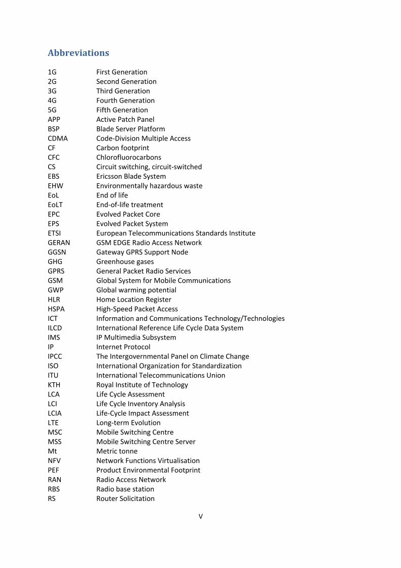
Abbreviations

1G First Generation 2G Second Generation 3G Third Generation 4G Fourth Generation 5G Fifth Generation APP Active Patch Panel BSP Blade Server Platform CDMA Code-Division Multiple Access CF Carbon footprint CFC Chlorofluorocarbons CS Circuit switching, circuit-switched EBS Ericsson Blade System EHW Environmentally hazardous waste EoL End of life EoLT End-of-life treatment EPC Evolved Packet Core EPS Evolved Packet System ETSI European Telecommunications Standards Institute GERAN GSM EDGE Radio Access Network GGSN Gateway GPRS Support Node GHG Greenhouse gases GPRS General Packet Radio Services GSM Global System for Mobile Communications GWP Global warming potential HLR Home Location Register HSPA High-Speed Packet Access ICT Information and Communications Technology/Technologies ILCD International Reference Life Cycle Data System IMS IP Multimedia Subsystem IP Internet Protocol IPCC The Intergovernmental Panel on Climate Change ISO International Organization for Standardization ITU International Telecommunications Union KTH Royal Institute of Technology LCA Life Cycle Assessment LCI Life Cycle Inventory Analysis LCIA Life-Cycle Impact Assessment LTE Long-term Evolution MSC Mobile Switching Centre MSS Mobile Switching Centre Server Mt Metric tonne NFV Network Functions Virtualisation PEF Product Environmental Footprint RAN Radio Access Network RBS Radio base station RS Router Solicitation

VI

SDN Software Defined Networking SGSN Serving GPRS Support Node UDM User Data Management WCDMA Wideband Code-Division Multiple Access WLAN Wireless Local Area Network WMO World Meteorological Organization

VII

List of Figures

Figure 1. LCA phases (ISO 2006a) ..................................................................................................... 5 Figure 2. Network domains - example for 3G (3GPP, 2014) ............................................................ 9 Figure 3. 3GPP architecture domains (Olsson, et al., 2013, p. 17) ................................................. 10 Figure 4. Blade Server Platform (BSP) 8100 ................................................................................... 13 Figure 5. System boundary ............................................................................................................. 16 Figure 6. Raw materials sub-model in GaBi ................................................................................... 31 Figure 7. Percentage distribution of raw materials by type, including packaging ......................... 32 Figure 8. Distribution of raw materials by type per group of parts ............................................... 32 Figure 9. Production sub-model with components models ........................................................... 36 Figure 10. Generic transportation model used for every transportation stage ............................ 40 Figure 11. EoL treatment model ..................................................................................................... 44 Figure 12. Impact distribution among life cycle stages .................................................................. 49 Figure 13. Contribution of different materials in the raw materials acquisition stage ................. 50 Figure 14. Distribution of environmental impacts among the production sub-stages .................. 52 Figure 15. Distribution of environmental impacts in the production stage among parts ............ 53 Figure 16. Distribution of environmental impacts among the different electricity mixes ............ 54 Figure 17. Distribution of environmental impacts among the different electricity mixes per unit of consumed energy ........................................................................................................................... 55 Figure 18. Contribution of formal recycling and landfill disposal per impact category ................. 56 Figure 19. Reduced impact of the transportation activities from the sensitivity analysis scenario ........................................................................................................................................................ 58 Figure 20. Results on the change of the potential impact of 1 kW electricity use in the climate change impact category (incl. biogenic carbon) from the sensitivity analysis ............................... 59

VIII

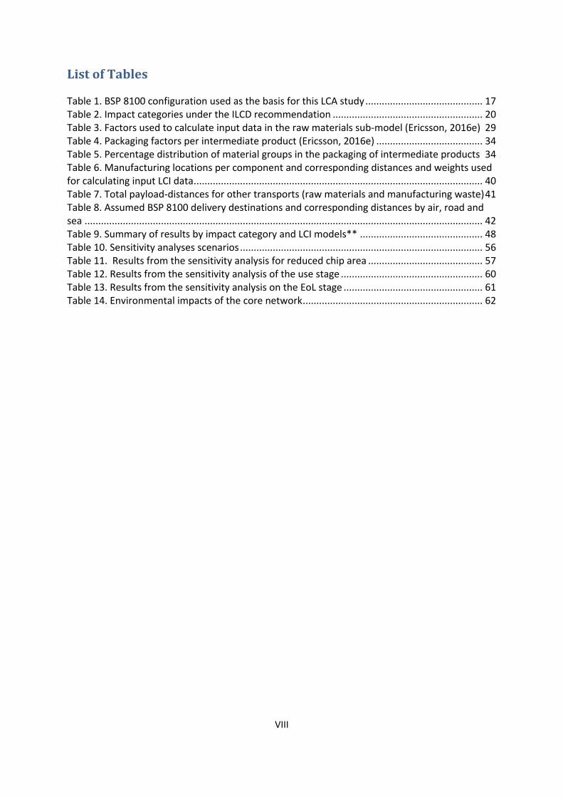
List of Tables

Table 1. BSP 8100 configuration used as the basis for this LCA study ........................................... 17 Table 2. Impact categories under the ILCD recommendation ....................................................... 20 Table 3. Factors used to calculate input data in the raw materials sub-model (Ericsson, 2016e) 29 Table 4. Packaging factors per intermediate product (Ericsson, 2016e) ....................................... 34 Table 5. Percentage distribution of material groups in the packaging of intermediate products 34 Table 6. Manufacturing locations per component and corresponding distances and weights used for calculating input LCI data .......................................................................................................... 40 Table 7. Total payload-distances for other transports (raw materials and manufacturing waste) 41 Table 8. Assumed BSP 8100 delivery destinations and corresponding distances by air, road and sea .................................................................................................................................................. 42 Table 9. Summary of results by impact category and LCI models** ............................................. 48 Table 10. Sensitivity analyses scenarios ......................................................................................... 56 Table 11. Results from the sensitivity analysis for reduced chip area .......................................... 57 Table 12. Results from the sensitivity analysis of the use stage .................................................... 60 Table 13. Results from the sensitivity analysis on the EoL stage ................................................... 61 Table 14. Environmental impacts of the core network .................................................................. 62

1

1. Introduction Mobile broadband radio access and bringing the Internet to mobile communications services is transforming the telecommunications industry, partly through a shift in the used technologies (Olsson, et al., 2009). Every year global mobile subscriptions with mobile network operators are growing with an average of 3 percent year-on-year, reaching 7.5 billion in the third quarter of 2016. Those associated with smartphones have surpassed mobile subscriptions for basic phones and account for 55% of all mobile subscriptions and are expected to go beyond 75% of all mobile subscriptions by 2022. At the same time, increased smartphone subscriptions combined with a rise in average data volume per subscriber are causing growth in mobile data traffic of 50% in one year. (Ericsson, 2016a) The carbon footprint (CF) of the information and communication technology (ICT) sector in Sweden has been increasing from 1990, when measurements started, until reaching its highest in 2010. However, later on a decrease has been taking place which is due to the improved energy performance of new devices and a shift from using personal computers and TV sets to smaller portable devices such as tablets and smartphones. (Malmodin and Lundén, 2016) In 2015, the carbon footprint (CF) of the Swedish ICT sector is estimated to be approximately 1.4 Mt CO2 eq,, or about 140 kg CO2 eq per capita, which covers about 1.2% of the overall Swedish CF from a consumption perspective, including embodied emissions of imported products and excluding exports. The estimated CF in 2015 is about 7% lower than that in 2010. (Malmodin and Lundén, 2016) The current decrease is a new observation, as an earlier forecast predicted an overall increase of the sector’s CF mainly due to the increase in number of subscriptions, which results from an increased number of devices, despite the improved energy efficiency of the network equipment and the reduced CF per device (Malmodin, Bergmark and Lundén, 2013). Increased environmental awareness and the focus on potential impacts associated with products have led to the development and then adoption of tools to comprehend these impacts and address them. One of these methods is Life Cycle Assessment (LCA) which has been included in the portfolio of international standards adopted by the International Organization for Standardization (ISO). (ISO 2006a, ISO 2006b) LCA belongs to a family of environmental systems analysis tools for environmental assessment (Baumann and Tillman, 2004). The increasing demand for communication and information flow pushes the ICT industry to expand its networks. As the development and spread of ICTs has raised concern about their environmental impact, the LCA methodology has been further adopted to complement the above standards for assessing the environmental performance of ICT goods, networks and services. This work was performed jointly by the International Telecommunications Union (ITU), the United Nations specialized agency for ICT, and the European Telecommunications Standards Institute (ETSI). Behind the motivation of ITU and ETSI to adopt LCA was not only global efforts to combat climate change, but also the fact that ICT differs from conventional products by having a double-edged nature: ICTs do have an environmental impact throughout their life cycle as any other product or service, on one hand, but on the other, through digital solutions they provide the means for efficiencies in lifestyle and in other sectors of the economy (e.g. videoconferencing, teleworking) as well as digital products instead of physical ones. (ITU, 2014; ETSI, 2015).

2

1.1 Previous studies on the environmental impacts of mobile networks and

core nodes A review of available literature on the application of LCA in ICT shows that different studies have been performed by various actors in the industry, often in collaboration with academia. No literature on core networks for mobile telecommunications was identified, as also shown in other research (Arushanyan, Ekener-Petersen and Finnveden, 2014), and for this reason mainly network LCAs associated with Ericsson have been cited below.

Some studies, as in Ercan (2013) and Ercan, et al. (2016), cover important aspects (primarily the carbon footprint) of the environmental impacts of different mobile devices. Others focus on services or parts of the ICT network system (Malmodin, et al., 2014; Malmodin and Lundén, 2016) or on the environmental impacts of fibre optic submarine cable systems (Donovan, 2009). According to ITU (2014), ICT networks are systems composed by different types of ICT goods and a network’s aggregated impact equals the sums of the impact from all the ICT goods comprising that network. Therefore, it is essential that the environmental impacts of all components of a network are studied. Scharnhorst, Hilty and Jolliet (2006) study the mobile network of the second and third generations, which are shortly introduced in Section 2.2 below. Their LCA focuses mainly on the end-of-life stage, but they also present results showing the main impact comes from the use stage and refer to the core network components as having comparatively low impact. The Swedish data transmission and IP core network was the focus of a case study by Malmodin, et al. (2012) with results on electricity consumption and global warming potential (GWP). The authors show that the results depend on the location of the network, as the electricity mix can substantially change the impact. In their study, applying a global mix instead of a Swedish one increased the overall impact more than three times and made the use stage account for more than 75% of the GWP instead of the initial less than 8%. Malmodin et al. (2014) point out the need for more up-to-date environmental assessment of ICT products based on more detailed, real measurements. In their work the authors focus on the overall operational electricity use and life-cycle-based carbon footprint corresponding to the extended ICT network in Sweden covering mobile and fixed access networks, data transmission and IP core networks, as well as user equipment connected to the networks. The study includes shared data transport networks, third-party enterprise networks, data centres, operator activities and the manufacturing of network infrastructures. Their results show that the carbon footprint of the extended Swedish ICT network is 1.5 Mt CO2

eq., or approximately 160 kg CO2 eq. per citizen. Applying a global electricity mix increases the carbon footprint more than twice. It is important to note that the study regards core nodes, which are the focus of the present Master’s thesis, as part of the access network, although in terms of mobile network infrastructure they belong to the core network (see Chapter 3). Therefore, their impact is included in the overall impact of the access network which in both electricity mix scenarios makes up less than 1/10 of the overall carbon footprint. Apart from that the study shows that the carbon footprint of the IP core network and data transmission

3

represents about 2.5% of the overall footprint for both electricity mix scenarios. (Malmodin et al., 2014)

1.2 Aim and objectives The aim of this project has been to estimate the potential environmental impacts of the core network for mobile telecommunications based on the LCA methodology, focusing on but not limiting itself to the impacts on climate change. For this purpose, it has had the following objectives:

To investigate the previous knowledge on the environmental impacts of the core network;

To identify the ICT equipment that corresponds to the core network;

To select and define the equipment to be assessed under this study;

To identify any hotspots of potential environmental impacts caused throughout the life cycle of the studied equipment by carrying out a study based on the LCA methodology;

From the results of the LCA study, to develop an estimate about the environmental impacts of the whole core network and of its usage by one mobile subscriber per year.

1.3 Problem Area and Specific Research Question This study falls into the general problem area of sustainable ICT and the environmental impact of ICT networks. The environmental impact of the core network for mobile communications is the specific problem area corresponding to the present study which addresses the following research questions:

What are the potential environmental impacts of the core network for mobile telecommunications from a life cycle perspective? Preliminary research and a literature review as the first of the above objectives have been conducted and their results are presented briefly in Section 1.1. Subsequently and after a consultation with LCA experts within Ericsson, the networking and telecommunications equipment and services company, it became clear that the industry in general and the company in particular have also identified a knowledge gap in that specific problem area, for which this study is initiated with Ericsson Research.

4

2. Theoretical Framework This chapter introduced LCA as the main methodology used for the purposes of this study. It also presents an overview of the mobile network, of the core network as part of it and of the equipment that provides its functionalities.

2.1 The LCA Methodology and Phases LCA is a method to assess quantitatively the environmental impacts of a product, including both goods and services, throughout its whole life cycle: from “cradle”, when raw materials are extracted from nature, through the stages of production and use, to “grave”, i.e. its final disposal back in nature. An LCA study models the whole industrial system behind a product or service, follows all consecutive and interlinked stages and includes all the inputs and outputs of that system. (Baumann and Tillman, 2004; ISO, 2006a, b) Each stage also includes transport and energy supply (ETSI, 2015). That holistic “cradle-to-grave” approach allows for avoiding problem shifting from one stage of the life cycle to another (Guinée, et al., 2004). LCA makes it possible to identify opportunities to enhance the environmental performance of products in different stages of their life cycles, provides relevant information to decision-makers in government, industry or the non-governmental sector and/or enables the definition of indicators of environmental performance (ISO, 2006a). Depending on the purpose of an LCA study, a “cradle-to-gate” approach can be also used, leaving out parts of the product system (Baumann and Tillman, 2004). A full LCA study usually requires an enormous amount of data, which makes it a time-consuming and, hence, expensive endeavour. For that reason, actors often use a simplified form of the method customized to serve the product and the purpose. (EEA, 1997) The technique finds different applications in the private sector. Among the most common ones is informing product development and improvement, as LCA allows for avoiding or minimizing foreseeable impacts. In a global market where consumers are becoming more environmentally conscious, LCA is often used for marketing purposes in order to communicate the environmental properties of products and services or for organization marketing, especially with companies following certain environmental standards or schemes. Often, the findings from LCA studies are also used by companies incorporating environmental aspects in their strategic business planning. (Baumann and Tillman, 2004; EEA, 1997) It is important to point out that nowadays companies are not only increasingly using LCA to cover key environmental aspects on a corporate level and collaborating with actors from in their value chains, but its use has expanded to whole industries trying to improve products and technologies (Hellweg and Milà i Canals, 2014). LCA finds wide application in public policy, as well, especially in product-oriented policy, waste management policies, taxation and subsidies, and other general policies. LCA can be used to inform the development of eco-labelling schemes or of environmental requirements in public and institutional procurement. The methodology can provide support for policy development in the field of waste management, energy, packaging, etc. Depending on the main purpose, both in the private and in the public sector LCA is sometimes used as the only decision support tool, but it is most commonly combined with other tools. (EEA, 1997)

5

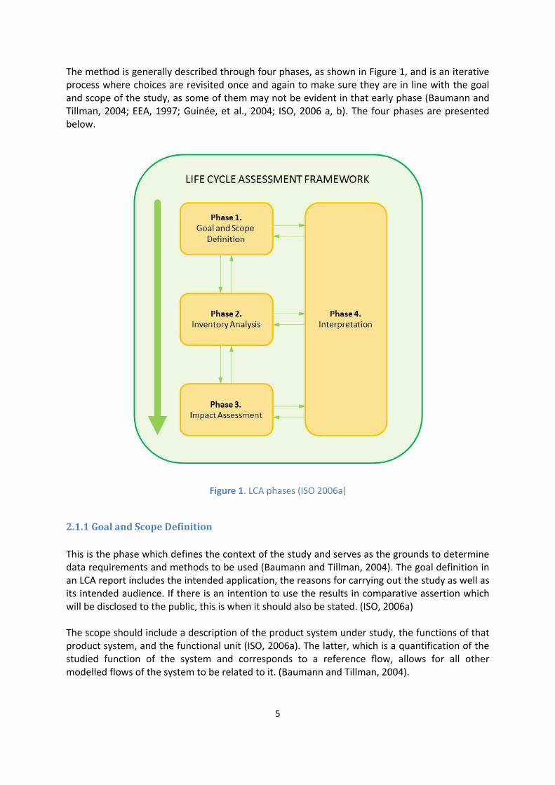
The method is generally described through four phases, as shown in Figure 1, and is an iterative process where choices are revisited once and again to make sure they are in line with the goal and scope of the study, as some of them may not be evident in that early phase (Baumann and Tillman, 2004; EEA, 1997; Guinée, et al., 2004; ISO, 2006 a, b). The four phases are presented below.

Figure 1. LCA phases (ISO 2006a)

2.1.1 Goal and Scope Definition

This is the phase which defines the context of the study and serves as the grounds to determine data requirements and methods to be used (Baumann and Tillman, 2004). The goal definition in an LCA report includes the intended application, the reasons for carrying out the study as well as its intended audience. If there is an intention to use the results in comparative assertion which will be disclosed to the public, this is when it should also be stated. (ISO, 2006a) The scope should include a description of the product system under study, the functions of that product system, and the functional unit (ISO, 2006a). The latter, which is a quantification of the studied function of the system and corresponds to a reference flow, allows for all other modelled flows of the system to be related to it. (Baumann and Tillman, 2004).

6

This LCA stage is where the system boundaries are defined by making a choice which processes will be included in the study, what methods of impact assessment will be used, as well as what types of environmental impacts will be considered (Baumann and Tillman, 2004). According to ITU (2014) and ETSI (2015), for defining the system boundaries of an LCA study in ICT all life cycle stages and unit processes associated with them should be included, i.e. unit processes related to raw material extraction and processing, ICT goods production, support goods production, site construction, use of ICT goods and support goods including also operator and service provider support activities, and end-of-life treatment. The system boundaries are outlined in their temporal, geographical and technological dimensions (Guinée, et al., 2004; Baumann and Tillman, 2004). The defined time horizon of the study includes the periods of production, use and waste treatment of the product system, makes it possible to identify the required data and set the desired data age and period of collection (Baumann and Tillman, 2004; Guinée, et al., 2004). The geographical boundaries matter as different life cycle stages may take place in different parts of the world, which may vary significantly in the types of infrastructure involved (Baumann and Tillman, 2004). The technology coverage, e.g. best available technology or the currently installed average one, in the geographical area should also be reported in relation to the goal (Guinée, et al., 2004). In this phase, the limitations of the study and the assumptions related to the system boundaries and/or lack of data should also be reported (Guinée, et al., 2004; EEA, 1997). Different aspects of the scope may undergo modification as the data and information is being collected (ISO, 2006a).

2.1.2 Life Cycle Inventory Analysis (LCI)

The life cycle inventory analysis is the phase of data collection for all the activities in the product system and its documentation which is often the most time-consuming portion of the whole LCA methodology. It includes finding relevant data on the amounts and types of inputs (raw materials, energy, other physical inputs, etc.) and outputs (products, emissions to air, water and soil, etc.), different types of transports, and energy use. If allocation between co-products that share the same process is to be performed, then data to support the allocation method chosen is also needed. During this stage qualitative data also needs to be collected on such details as, for example, applied technology of a process, its location, etc. (Baumann and Tillman, 2004; EEA, 1997) As a first step of this stage a flowchart of the system is created depending on its system boundaries, which helps identify the required data. As LCI is an iterative process, the modelled flows may be revisited and modified with the collection of more data on the system. As in practice data gaps are inevitable, all estimates and assumptions which aim to fill those should be duly justified and documented for transparency. This is where recycling rates and energy use are accounted for. To improve the overall data quality, validation of data should be conducted. After all data is collected, the LCI calculations are performed by normalising the inputs and outputs individually and then linking them based on the activities in the flowchart. Thus, the environmental loads of the system are quantified in relation to the functional unit (Baumann and Tillman, 2004; EEA, 1997; ISO, 2006b).

7

2.1.3 Life Cycle Impact Assessment (LCIA)

After the environmental loads have been quantified in the LCI, the aim of the LCIA is to describe their environmental impacts such as acidification, human toxicity, ecotoxicity, effect on biodiversity, etc. which belong to three categories: resource use, human health, and ecological consequences. In this way, the results are “translated”, made more comprehensible and easier to communicate. In the LCIA, the environmental loads can be grouped, thus reducing the number of parameters and making the results more readable and easier to perceive. (Baumann and Tillman, 2004) This stage consists of a mandatory part and a few optional steps. Impact category definition, classification and characterisation are required elements in every LCIA. The first one is the identification and selection of environmental impacts relevant to the goal and scope definition in categories. Normally, it is based on the information from the inventory analysis taking into account different factors (completeness, practicality, environmental relevance, independence, etc.). Classification is the sub-phase of assigning the different LCI results to their corresponding categories. With characterisation, the extent of the impact is calculated per every category. This is performed by using characterisation/equivalency factors (other terms are also used). This is the sub-phase where environmental loads are transformed into impact. For this purpose, scientifically-based characterisation methods are used. (Baumann and Tillman, 2004; ISO, 2006b) In LCIA, the optional elements are normalisation, grouping, weighting and data quality analysis. In the normalisation steps the characterisation results are related to a reference value. This is, in other words, putting the results into context to see their magnitude. Grouping involves sorting and ranking impact categories, for instance, in terms of priority or of scale of impact (local, regional, global). Weighting is the process where the different environmental impacts are weighted according to their importance in relation to each other. Numerical factors based on value choices are applied to convert the results. Different types of methods (panel, monetization, etc.) are used. Normalisation of results on the level of the whole core network has been undertaken under this study and is presented in section 6.2.

2.1.4 Life Cycle Interpretation

The interpretation is the final stage of the LCA process where raw results from the LCI and the LCIA are “refined” to extract valuable, comprehensible and useful information for the target audience. The results presented may vary depending on the intended users. In this phase, the robustness of the results and the model are tested and evaluated through relevant methods such as uncertainty or sensitivity analyses which allow for understanding better the LCIA results. Thus, significant differences or negligible LCI may be identified. This is the part for making conclusions and recommendations that are consistent with the requirements set within the goal and scope definition. A critical review of the study also takes places in this LCA stage. The interpretation phase is another iterative process and is being revisited and revised along with the progress on the other LCA stages (Baumann and Tillman, 2004; EEA, 1997; ISO, 2006b).

8

2.1.5 Methodology Limitations

LCA is based on a model representation, and therefore it is a “relative expression” of potential environmental impacts and does not assess actual impacts. This limitation is even more relevant for complex products systems from the ICT industry, as it is “virtually impossible” to collect enough data for an assessment that reflects the actual performance of a studied system, which is why results always contain model and scenario uncertainty. (ETSI, 2015, p. 149) Uncertainties result from the simplified modelling of complex environmental cause-effect systems and to the large share of measured and simulated data. In LCA, data gaps are a problem in the early stages of technology development which brings a limitation in the application of the methodology. Regionalization in LCA increases its relevancy on one hand, but on the other, practitioners still face difficulties in matching regionalized impact-assessment methods with regionalized resource flows and emissions. (Hellweg and Milà i Canals, 2014). Another limitation is the fact that LCIA addresses only the environmental issues defined in the goal and scope, and therefore, it does not assess all the environmental issues relevant to the studied product system (ISO, 2006a).

2.2 The Mobile Network and Its Core The mobile telecommunications system architecture can be structured according to either physical or functional characteristics. The physical aspects of the architecture are modelled using a domain concept, and the basic architecture is split between the user equipment and the infrastructure (see Fig. 2). The network infrastructure is further split into the Access Network Domain, the one being directly connected to the user equipment, and the Core Network Domain. The core network, which is the focus of the present study, consists of infrastructure entities providing support for the network features and telecommunication services covering functions such as the management of user location information, control of network features and services, the transfer mechanisms for signalling (switching and transmission) and for user generated information. The core network is divided into the serving network, the home network, and the transit network. (3GPP, 2014) The serving network domain is the one connected to the access network and routes calls and transports user data from source to destination, thus providing the functions that are local to the user’s access point and that change location while the user is moving. For user-specific data and services the serving network interacts with the home network domain, and for non-user-specific data and services – with the transit network. The home network manages subscription information, contains user specific data and handles the core network functions that are carried out at a permanent location regardless of the user’s location/access point. The transit network manages the communication between the serving network and the remote party. (3GPP, 2014)

9

Figure 2. Network domains - example for 3G (3GPP, 2014)

2.2.1 The Development of Mobile Communication Technologies and Standards

The development of telecommunications has led to evolution of different technology generations and standards. The analogue radio system was the first one (1G), followed by the first digital mobile systems (2G), then the first mobile systems dealing with broadband data (3G). Deployment of mobile communication technologies has later introduced the fourth generation through Long-Term Evolution (LTE) which provides better speed for broadband data. The industry is currently working on the 5G radio access technology which is needed to support a network providing access not only to mobile devices, but also wide-scale communication for machines such as smart home appliances, smart-grid devices, etc. and connected sensors. (Dahlman, E., Parkvall, S. and Sköld, J., 2014) With this technological development many radio standards were created defining the technologies to be implemented by the industry. At the beginning, this process started on a national or regional level, which brought about the development and deployment of different technologies defined within different standards organizations. (Dahlman, E., Parkvall, S. and Sköld, J., 2014) The most common radio standards include GSM (Global System for Mobile Communications) for 2G and WCDMA/HSPA (Wideband Code-Division Multiple Access/ High-Speed Packet Access) for 3G (Olsson, et al., 2013). The second-generation technology, GSM being the most common, was based on circuit switching and used a cellular network to provide voice services. After the usage of the Internet became common in the 1990s, a demand to enable it on mobile devices pushed the industry’s evolution to HSPA, belonging to the third-generation in mobile communications technology, which delivers high data rates, followed by the fourth generation LTE. (Olsson, et al., 2013; Dahlman, Parkvall and Sköld, 2014)

10

2.2.2 The Development of the Core Network

Every operation with a mobile device goes through the core network. It is that part of the physical mobile network which controls the network features and telecommunication services, handles the management of user location information and the transfer mechanisms, both switching and transmission, for signalling and for user generated information (3GPP, 2014). The different standardized radio access technologies also involved different core networks (Olsson, et al., 2013). Standardization and mobile technology development in the past was taking place regionally, but with the shift from GSM to WCDMA/HSPA there was a need to enable standardization on a global level. This made the industry initiate 3GPP, a global forum which handled the standardization of both the radio access network (RAN) and the core network for WCDMA/HSPA. The new core network was based on GERAN with some updates, mainly the addition of some interfaces. (Olsson, et al., 2013) GSM has a core network characterized by nodes, i.e. points of intersection/connection, for circuit-switched telephony. The Mobile Switching Centre (MSC) and the Home Location Register (HLR) are the main components of the GSM core network. Later, the General Packet Radio Services (GPRS) system was created as an addition to the GSM system to support IP traffic, and it demanded a packet-switched core network. It uses a network-based mobility scheme and relies on tracking movements of end-user devices. This led to the introduction of two new core nodes: Serving GPRS Support Node (SGSN) and Gateway GPRS Support Node (GGSN) which handle user data traffic. (Olsson, et al., 2013) Nowadays, when the telecommunications industry is using data and voice services based on Internet Protocol (IP) and packet-switched technologies, the core network serves as the link between the high-speed radio access network and mobile Internet services. This required a core network designed for high-bandwidth services and brought the development of the Evolved Packet Core (EPC). Before EPC, there were different core network architectures corresponding to different radio access technologies. The EPC involves simplified all-IP architecture and handles multiple radio access technologies which provide mobility between different radio standards, as well as other network technologies such as WiFi or fixed access. It is part of the Evolved Packet System (EPS) which includes the radio access, the core network and the terminals that cover the whole mobile system. (Olsson, et al., 2013)

2.2.3 State-of-the-art Mobile Technology and the Current Core Network

Figure 3. 3GPP architecture domains (Olsson, et al., 2013, p. 17)

11

According to Ericsson (2016a), mobile communications will continue migrating from the globally prevailing GSM/EDGE-only subscriptions in 2016 to expected dominating LTE ones from 2019. Although GSM-only subscriptions currently hold the largest share, in 2022, WCDMA-subscriptions are expected to outnumber them more than three times and LTE subscriptions – more than five times to represent the largest share. A subscriber is every user of the mobile network of a given operator, and one person may hold more than one mobile subscription. Developed markets are already shifting towards the newer technologies, but in developing markets GSM is still viable because of the low cost of corresponding mobile phones and subscriptions. In any case, as a fallback the majority of WCDMA and LTE subscribers will still have access to GSM. (Ericsson, 2016a) As mentioned in Section 2.2.2, services based on multiple radio access technologies would be supported by a network defined by 3GPP specifications, as shown in Figure 3, and including the EPC. That network includes the RAN domains of the second (GSM), third (WCDMA) and fourth (LTE) generations of networks, as well as packet data access networks not covered by 3GPP standardization such as wireless local area networks (WLAN), fixed network accesses, etc. As illustrated in Figure 3, the core network consists of several domains: Circuit Core, Packet Core and IMS, which work together. The subscriber data management domain facilitates roaming and mobility between and within the different domains and handles coordinated subscriber information. The Circuit Core provides support for circuit-switched services over GSM and WCDMA. The Packet Core functions support packet-switched services over GSM and WCDMA, as well as over LTE and non-3GPP access networks. The IMS domain covers functionalities that support multimedia sessions and uses the IP connectivity provided through the Packet core. The core network also covers a subscriber data management domain. (Olsson, et al., 2013) Another development has been taking place with mobile networks recently, affecting the core network. The growing communication demand makes networks need an increasing variety of hardware which requires more space, power and trained maintenance staff. Handling these networks based on dedicated hardware is resource-intensive, cannot correspond to the accelerated pace of innovation and slows down service providers in offering dynamic services. That is why the industry has started working on virtualising network functions on multi-purpose network platforms to make them dynamically configurable and responding automatically to the needs of the traffic and the services it handles. For that purpose, the industry uses two complementary technologies: Software Defined Networking (SDN) and Network Functions Virtualisation (NFV). (ETSI, n.d.) SDN allows running networks through software and enables the initialization, control, change and management of networks dynamically through open interfaces by separating the control plane and the forwarding place (Haleplidis, et al. 2015), while NFV is the “principle of separating network functions from the hardware they run on by using virtual hardware abstraction” (ETSI, 2014, p. 7). While SDN focuses on optimising the network, NFV decouples the network services from specific hardware to make them run in software (SDxCentral, n.d.a). Nowadays operators have the flexibility to virtualize only parts of their networks. Also these technologies allow them to share infrastructure for multiple networks while still controlling their own share. (SDxCentral, n.d.b)

12

2.2.4 Generic Core Network Equipment

Nowadays the core network infrastructure is built on servers hosting multiple applications that provide the needed functionalities. This section introduces the company equipment that comprises a great part of the infrastructure for core network functionalities and is the focus of this LCA-based study. The Ericsson Blade System (EBS) is a flexible and modular concept used for the core network of several telecommunications systems with different interfaces and processing capacities. It allows flexibility in configuration depending on the need for hosting specific applications or traditional circuit switching. (Cronebäck, 2013) Before EBS, different core network applications used to run on different hardware configurations, while currently there is a trend in migrating most of those applications to the EBS (Blomqvist, 2015). The Ericsson BSP (Blade Server Platform) 8000 is a state-of-the-art, standalone server product family that hosts one or many applications (Ericsson, 2015b). It belongs to EBS, and while BSP 8000 is the name of the product family, BSP 8100 indicates the first generation of the product (Ericsson, 2015b). BSP 8100 houses multiple software applications covering the functionalities of the Packet Core, Mobile Switching Centre Server (MSS), IP Multimedia Subsystem (IMS), charging and activation, User Data Management (UDM), and Router Solicitation (RS) (Ericsson, 2016d). BSP 8100 refers to the whole system including both hardware and software. BSP 8100 (see Figure 4) has no predefined configuration, as the exact configuration differs with each order, as it depends on the applications to be used and their dimensioning (Ericsson, 2016b). The hardware includes a cabinet, subracks with switch boards for system control, and a configuration-specific number of processor boards (blades). The cabinet also contains power and fan modules, cables as well as any application-specific boards. According to Blomqvist (2015) and Wägmark (2015a), BSP configurations are never delivered as fully equipped cabinets and free space in the subracks is left for expansions. In such case, dummy boards are used to fill all empty slots in the subracks to provide adequate cooling. Two dummy units are needed to cover the space for one processor blade. (Ericsson, 2016b) Decoupling hardware and network functions affects the core network too, and BSP takes part in the virtualization process. Since 2016, Ericsson has been gradually introducing different virtualized application to run on BSP 8100. This provides more flexibility and reduces the need for hardware, but it has some impact on the applications’ capacity. (Magnus, 2015; Ericsson, 2016d)

13

Figure 4. Blade Server Platform (BSP) 8100 (Ericsson, 2015b)

14

3. Goal and Scope The following chapter describes the goal and scope of the study on the core network based on the LCA methodology and defines the boundaries of the system under assessment. It presents details on the functional unit, as well as on the methods, assumptions and limitations involved.

3.1 Goal The goal of the present LCA-based study is to assess the potential environmental impacts of a representative configuration of BSP 8100 used as core network equipment with the purpose of analysing the significant inputs of materials and energy and their emissions throughout the life cycle of the system and identifying the activities with the most significant potential environmental impact. This would later allow estimating the potential environmental impacts of the core network itself which is the aim of this study.

3.1.1 Target Audience

In the context of sustainable development, with a growing number of mobile subscriptions and an expanding network capacity, up-to-date knowledge on the environmental impacts of all parts of the mobile network is of interest not only to Ericsson as a global company in ICT, but to the whole industry, policy makers and academic researchers. Yet, as shown in Section 1.1, little is known of the environmental impacts of the core network. Therefore, the results of this study will be of interest to researchers in the fields of both ICT and the environmental performance of products and services.

3.1.2 Applicability of the Study

This study enables an understanding regarding the contribution of the core network to the overall potential environmental impacts of the state-of-the-art mobile network and in which stages of its life cycle core-network hardware equipment brings the most significant environmental impacts. This would allow identifying the activities in the life cycle of the studied system where there might be opportunities for improvement in terms of environmental performance and can provide information to stakeholders as assistance to their policy choices. This study, as being based on a complex product system involving products developed in different generations and combining new services and solutions (e.g. virtualization), can be used in the future to track potential impacts and improvements of these new product generations and solutions. (ETSI, 2015, p. 149). This study, together with other LCA studies on the environmental impacts of the rest of the mobile network, may be of interest to end-users, especially environmentally conscious consumers, and can be used to raise environmental awareness.

3.2 Scope In this section, a description of the system under study is provided with its boundaries and delimitations, and the functional unit is defined. The data requirements and quality are

15

introduced, as well as the methods for inventory analysis and for impact assessment, and the software used for the LCA modelling. These are followed by an overview of the study-wide assumptions, simplifications and limitations, and by a short presentation of the adopted critical review procedure.

3.2.1 System Description

The system covered by this LCA involves a set of products that represent a generic type of a blade server platform used by Ericsson in building mobile networks. The system is modelled from cradle to grave including all life-cycle stages from raw material acquisition, production, and use to end-of-life treatment, and it also comprises the transportation activities corresponding to the above stages for Ericsson BSP 8100 (see Figure 4 for product system). Further information about the system is presented in Section 3.2.3.3 and Chapter 4.

3.2.2 Functional Unit

This LCA focuses on studying the function of providing core network services through specific hardware equipment. According to ITU (2014), ICT networks are systems composed by different types of ICT goods and a network’s aggregated impact equals the sums of the impact from all the ICT goods comprising that network. Therefore, assessing the potential environmental impacts of an average product system that provides coverage for a certain number of subscribers and has certain electricity consumption would allow for estimating the potential environmental impacts of the core network which is the aim of the present study. For the above goal, the functional unit is defined as:

use of one representatively equipped BSP 8100 cabinet for five years, as further presented in Table 1 and explained in section 3.2.3.3 and Appendix A. It is assumed based on a network dimensioning model used by Ericsson (Singh, 2016) that such a configuration covers more than 1 million subscribers. Details on how the functional unit and the results on the potential environmental impact are used as reference to estimate the environmental performance of the core network are presented in Chapter 6.

3.2.3 System Boundary

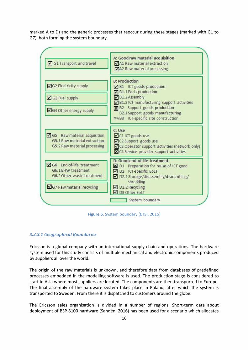
The present study covers the complete life cycle, from cradle to grave, of a configuration of the BSP (see further details below in 3.2.3.3 Technological Boundaries). The boundaries of the considered system begin with nature and the extraction of raw materials and finish with the end-of-life treatment and the corresponding emissions to nature, i.e. emissions to air, water, solid waste and other releases (see Figure 5). It is important to note that although the aim of the overall study presented in this report is to estimate the potential environmental impacts of the core network, the part of it based on LCA only assesses the potential impacts of a specific product system, hence it is an LCA on ICT equipment/goods and not on ICT networks and services in terms of the definitions and requirements set by ETSI (2015) and ITU (2014). The system boundaries of this study have been defined based on the accessibility of data in relation to the time constraints of the study itself. Figure 5 (adapted from ETSI, 2015) shows the life cycle stages included in this study (on the right

16

marked A to D) and the generic processes that reoccur during these stages (marked with G1 to G7), both forming the system boundary.

Figure 5. System boundary (ETSI, 2015)

3.2.3.1 Geographical Boundaries

Ericsson is a global company with an international supply chain and operations. The hardware system used for this study consists of multiple mechanical and electronic components produced by suppliers all over the world. The origin of the raw materials is unknown, and therefore data from databases of predefined processes embedded in the modelling software is used. The production stage is considered to start in Asia where most suppliers are located. The components are then transported to Europe. The final assembly of the hardware system takes place in Poland, after which the system is transported to Sweden. From there it is dispatched to customers around the globe. The Ericsson sales organisation is divided in a number of regions. Short-term data about deployment of BSP 8100 hardware (Sandén, 2016) has been used for a scenario which allocates

17

the use stage among these regions taking into consideration regional electricity mixes wherever available in the database of GaBi, the LCA software used to model the product system. The model accounts for local 83% recycling of the equipment nearby the chosen locations considering the same electricity mix as for the use stage and transportation by truck.

3.2.3.2 Temporal Boundaries

Although the functional design lifetime criterion for processor boards is 20 years (Wägmark, 2015b), a commercial lifetime of 5 years is considered for the purposes of this study based on expert opinions at Ericsson due to rapid technology development and upgrades of deployments. This period is adopted as the duration of the use stage in this study. Generic data with varying age has been obtained from databases available with the LCA modelling software for raw materials, some production processes, electricity, transportation, fuels, etc., however, in pursuit of using the latest data available. A list of all data sources with their corresponding age is provided in Appendix B. Data goes as far back as 1993 and due to the time constraints of this study no further analysis has been performed in connection with its age. Whenever data was available, the production stage in this study has been modelled with data from an internal LCA study performed by Ericsson on the potential environmental impacts of a radio base station (RBS), a component of the access network which is represented by similar hardware configurations (Ericsson, 2016e). The age of this data is unknown; however, its collection was initiated in 2011. Data gaps have been filled with the above-mentioned generic data from GaBi. On the EoL stage data gaps have been addressed by using data on the EoL treatment of ICT equipment based on Liebmann (2015) and used in Ercan, et al. (2016).

3.2.3.3 Technological Boundaries

The technological boundaries of this study are limited to one specific BSP 8100 configuration. As customers receive customized configurations depending on the needs of their networks in terms of functionalities, capacity, subscriber base, coverage, selected core network applications, etc., this study is based on a representative configuration in terms of hardware and not of functionality. As listed in Table 1, the studied configuration consists of one cabinet, three subracks housing a number of blades of different capacity (to two-thirds of the subracks’ slot capacity). Further details regarding the product system configuration are internal to Ericsson and available in Appendix A.

Table 1. BSP 8100 configuration used as the basis for this LCA study

Part Quantity

Cabinet 1 pcs

Subrack 3 pcs

Switch boards (two types) 12 pcs

Processor boards (three types) 24 pcs

Dummy units 24 pcs

Cables 82 kg

18

The process of recovery and recycling of materials from the product system is included in the end-of-life treatment stage. The BSP 8100 software development is not modelled on its own but forms part of the Ericsson activities for which a generic LCA models have been developed within the company to be used in different product LCAs (Ericsson, 2016e). The operation of software is included in the energy consumption of the use stage. Ericsson activities and capital goods, e.g. computers used by Ericsson, as well as the assembly process are considered based on earlier LCA studies (Ericsson, 2016e), see 4.4.3.3. Operator activities are excluded from this study (see Section 4.1). The virtualization of applications on BSP 8100 remains outside the technological boundaries of this LCA, as it is still to be introduced for most of those applications which deters the collection of data. As explained by Blomqvist (2015), virtualization allows core network applications to run on virtual machines, thus reducing the need for dedicated hardware, but this makes the applications lose capacity. The duration of this study is another reason for not considering those within the system boundaries.

3.2.4 Methods for Inventory Analysis

The methods for inventory analysis in this LCA study include system modelling with of the activities and flows identified within the system boundaries following all life-cycle stages presented in Figure 5, data collection and calculation. The system modelling was based on internal Ericsson literature and products documentation and on the professional experience of Ericsson experts. Data has been collected and documented for all the activities in the product system. Assumptions for data gaps have been made based on the collection of qualitative data about the product system. The process was iterative, and the system model, as well as the goal and scope of the study, have been revisited, refined or revised according to new findings. The data has then been normalized for all activities, and flows linking these activities have been calculated, all using the functional unit as reference or units. The flows within and crossing the system boundaries have been automatically calculated by the specialized GaBi 7.0 software used to model the whole system and to facilitate the LCA. The software also calculates the corresponding environmental loads. Data has been validated by comparing between different internal data sources, and where possible, comparing with external ones. Data calculations have been performed to account for any allocation required before the input of data into the LCA software. Energy use has been accounted for in every life-cycle stage depending on identified energy flows by using the databases available with the GaBi software on different fuels and energy sources. Due to the time constraints of this study and the complexity of the product system, Ericsson experts advised that data suppliers would only be internal company sources and available public sources. Suppliers of materials and components in the different life-cycle stages would not be contacted for data collection. Instead, as mentioned above, primary data from another LCA study (Ericsson, 2016e) would be used, as there is an overlap of product types, suppliers and their activities.

19

3.2.5 Allocation Procedure

The ISO standards define allocation as “partitioning the input or output flows of a process or a product system between the product system under study and one or more other product systems” (ISO, 2006b, p. 4). As Guinée, et al. (2004) point out, allocation is one of the most sensitive issues in LCA. In terms of allocation, this study follows the procedures set by the ETSI standard (ETSI, 2015, pp. 49-50) except for the EoL stage and recycling. Following the both the ISO (2006a; 2006b) and ETSI (2015) standards, allocation has been avoided as much as possible by increasing the level of detail. Where impossible to avoid, allocation has been performed by partitioning the inputs and outputs based on the physical relationship between them, most often expressed by mass (or by surface area which is more relevant with IC and PCB). Further details on where in the system allocation issues have been encountered and could not be avoided, how allocation has been performed while processing input and output data and why that method has been chosen are available below in Section 4.5. It is important to note that allocation procedures are also embedded in the secondary GaBi data used in the modelling to an unknown extent, for example, partitioning inputs and outputs when accounting for electricity produced together with thermal energy from one fuel source.

3.2.6 Methods for Impact Assessment

The methodology for impact assessment in this LCA follows the requirements of the ISO14044 standard (ISO, 2006b) and the ILCD Handbook guidelines (European Union, 2010a), as recommended by ETSI (2015). Impact categories have been defined following the recommendations of the International Reference Life Cycle Data System (ILCD) about the methodologies that has been evaluated as the best within every impact category (Thinkstep, n.d.; European Union, 2011). These have been applied as impact assessment methods, since they have been used by Ericsson for recent LCA studies. The processes of classification and characterisation are automated, as the characterisation database is provided in the GaBi software. The results for the potential environmental impacts of the product system are used to estimate the potential environmental impacts for the whole core network, and the results of that estimation have been normalized to relate the magnitude of the potential impact of the whole mobile network.

3.2.7 Definition of Impact Categories and Characterisation Factors

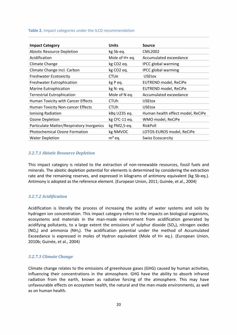
For the purpose of this study the characterisation models following the recommendations of the ILCD at midpoint level have been applied (European Union, 2011). The criteria and evaluation procedure to recommend these methods for the impact categories in Table 8 are presented in detail in the ILCD Handbook (European Union, 2011). The ILCD Recommendations characterisation database is provided with the GaBi software.

20

Table 2. Impact categories under the ILCD recommendation

Impact Category Units Source

Abiotic Resource Depletion kg Sb-eq. CML2002

Acidification Mole of H+ eq. Accumulated exceedance

Climate Change kg CO2 eq. IPCC global warming

Climate Change incl. Carbon kg CO2 eq. IPCC global warming

Freshwater Ecotoxicity CTUe USEtox

Freshwater Eutrophication kg P eq. EUTREND model, ReCiPe

Marine Eutrophication kg N- eq. EUTREND model, ReCiPe

Terrestrial Eutrophication Mole of N eq. Accumulated exceedance

Human Toxicity with Cancer Effects CTUh USEtox

Human Toxicity Non-cancer Effects CTUh USEtox

Ionising Radiation kBq U235 eq. Human health effect model, ReCiPe

Ozone Depletion kg CFC-11 eq. WMO model, ReCiPe

Particulate Matter/Respiratory Inorganics kg PM2,5-eq. RiskPoll

Photochemical Ozone Formation kg NMVOC LOTOS-EUROS model, ReCiPe

Water Depletion m³ eq. Swiss Ecoscarcity

3.2.7.1 Abiotic Resource Depletion

This impact category is related to the extraction of non-renewable resources, fossil fuels and minerals. The abiotic depletion potential for elements is determined by considering the extraction rate and the remaining reserves, and expressed in kilograms of antimony equivalent (kg Sb-eq.). Antimony is adopted as the reference element. (European Union, 2011; Guinée, et al., 2004)

3.2.7.2 Acidification

Acidification is literally the process of increasing the acidity of water systems and soils by hydrogen ion concentration. This impact category refers to the impacts on biological organisms, ecosystems and materials in the man-made environment from acidification generated by acidifying pollutants, to a large extent the emissions of sulphur dioxide (SO2), nitrogen oxides (NOx) and ammonia (NH3). The acidification potential under the method of Accumulated Exceedance is expressed in moles of Hydron equivalent (Mole of H+ eq.). (European Union, 2010b; Guinée, et al., 2004)

3.2.7.3 Climate Change

Climate change relates to the emissions of greenhouse gases (GHG) caused by human activities, influencing their concentrations in the atmosphere. GHG have the ability to absorb infrared radiation from the earth, known as radiative forcing of the atmosphere. This may have unfavourable effects on ecosystem health, the natural and the man-made environments, as well as on human health.

21

The Intergovernmental Panel on Climate Change (IPCC) has developed a characterisation model that calculates the radiative forcing of all GHG, which is branded as their global warming potential (GWP). It is measured in kilograms of carbon dioxide equivalents (kg CO2 eq.). This midpoint impact category is mandatory for studies in ICT, and IPCC characterisation factors should be used with the timeframe of 100 years. (European Union, 2010b; Guinée, et al., 2004; ETSI, 2015) The GaBi software divides climate change under the ILCD recommendations into two impact categories: one without and one including the potential impact of biogenic carbon (PE International, 2016).

3.2.7.4 Freshwater Ecotoxicity

This category addresses the impact on freshwater ecosystems from the emission of toxic substances in the air, water and soil. The characterisations model and factor should account for the pollutant’s fate in the environment, species exposure and the differences in toxicological response (likelihood of effects and severity). Under the USEtox method they are expressed in comparative toxic units for ecosystems (CTUe). (European Union, 2010b; Guinée, et al., 2004)

3.2.7.5 Eutrophication

The eutrophication impact categories address the potential impacts of excessive levels of macronutrients, mostly nitrogen (N) and phosphorus (P) in the environment. This may lead to increased biomass production and shift in species compositions. (European Union, 2010b; Guinée, et al., 2004) The addition of nutrients in aquatic systems fertilizes plants, thus changing the species composition in the ecosystem, Blooming algae prevent light from penetrating deeper into the water which changes the conditions for photosynthesizing plants and for predatory fish which need it to catch their prey. The additional biomass formation causes greater deposits of dead and degrading algae, which results in oxygen depletion near the bottom of the water. All these effects gradually change the species composition and the function of the affected aquatic ecosystem. (European Union, 2010b) Freshwater and marine ecosystems are both exposed to emissions of nitrogen- and phosphorus-containing compounds in the water. Marine environments and very large lakes can also be significantly exposed to air-borne emissions of nitrogen oxides. In general, freshwater ecosystems are affected mostly by phosphorus; hence the eutrophication potential after the ReCiPe method is expressed in kilograms of Phosphorus equivalent (kg P eq.). Marine eutrophication, on the other hand, is caused mostly by nitrogen, so it’s the eutrophication potential in marine environments is measured in kilograms of Nitrogen equivalent (kg N eq.). (European Union, 2010b) In terrestrial ecosystems, the addition of nutrients first changes the vegetation composition by favouring the growth of species which benefit from the higher levels of nutrients. A changed plant community then leads to impacts on other species in the ecosystem. Terrestrial eutrophication is associated mainly with nitrogen compounds from combustion processes and ammonia from agriculture. The eutrophication potential is expressed in accumulated exceedance in moles of nitrogen equivalent (mole of N eq.). (European Union, 2010b; 2011)

22

3.2.7.6 Human Toxicity

This impact category concerns the effects of toxic substances present in the environment on human health. It looks into emissions in air, water and soil. The used method USEtox was developed by a task force within the UNEP-SETAC Life Cycle Initiative. ILCD recommends the calculation of separate midpoint factors for cancer and non-cancer effects, as well as treating particulate matter/respiratory inorganics and ionizing radiation as separate impact categories (see below). In the GaBi software, human toxicity under the ILCD Recommendations is assessed in two separate categories depending on the toxicological effects, in this case cancer effects and non-cancer effects (e.g. memory loss), associated with the emission of certain chemicals. Human toxicity reflects the concentration of these chemicals at human uptake level in comparative toxic units for humans (CTUh). (European Union, 2010b; Guinée, et al., 2004; ITU, 2014)

3.2.7.7 Ionising Radiation

This is the impact category that covers the impacts from releases of radioactive materials to the environment and the direct exposure to radiation. Impacts can affect both human health and ecosystems and is expressed in terms of the numbers of atoms disintegrating per unit time, the measuring unit of one Becquerel meaning one disintegration per second. This characterisation model focuses on the effects on human health expressed in equivalent uranium radiation measured in kilo Becquerel (kBq U235 eq.). (European Union, 2011; Guinée, et al., 2004)

3.2.7.8 Ozone Depletion

This impact category refers to the thinning of the stratospheric ozone layer due to man-made emissions of ozone depleting substances. Ozone molecules are destroyed by chlorine atoms in chlorofluorocarbons (CFC) and bromine atoms in halons. Stratospheric ozone stops harmful solar ultraviolet UV-B radiation from penetrating lower in the atmosphere and reaching the earth’s surface. If not absorbed, UV-B radiation can harm human and animal health, terrestrial plants and aquatic ecosystems. The characterisation model is developed by the World Meteorological Organization (WMO) defines the ozone depletion potential of different gases, whose emissions are measured in kilograms of chlorofluorocarbons-11 equivalents (kg CFC-11 eq.) as reference unit. (European Union, 2010b; Guinée, et al., 2004)

3.2.7.9 Particulate Matter/Respiratory Inorganics

This impact category relates to the ambient concentrations of particulate matter increased by the emissions of primary and secondary particulates. Particulate matter is measured in different ways, one of them being depending on its diameter: particulate matter less than 10 microns in diameter (PM10), particulate matter less than 2.5 microns in diameter (PM2.5), particulate matter less than 0.1 microns in diameter (PM0.1) or total suspended particulate matter.

23

The model reflects the influence on intake and the subsequent damages to human health. The characterisation factor accounts for the pollutant’s environmental fate (relating emission flows to the mass in the air), exposure (the intake rate per change in mass in the environment) and dose-response (relating the change in intake to the change in morbidity/mortality. Emissions are expressed in kilogram of particulate matter 2.5 microns equivalent (kg PM2,5-eq.). (European Union, 2010b; Guinée, et al., 2004)

3.2.7.10 Photochemical Ozone Formation

Photochemical ozone formation concerns the formation of ozone photochemically by the action of sunlight on some air pollutants such as carbon monoxide (CO) and volatile organic compounds (VOCs) in the presence of nitrogen oxides (NOx). The ReCiPe method used relates to the harmful effects on human health. Emission factors are measured against the reference unit of kilogram of non-methane volatile organic compound equivalent (kg NMVOC). (European Union, 2010b; Guinée, et al., 2004)

3.2.7.11 Water Depletion

ILCD recommends different categories of methods for resource depletion, and one of them is for water. The reason is that water depletion is location-specific; there is no global market for water as there is for other resources (e.g. oil, minerals) and no global scarcity, and therefore the characterisation model needs to consider that regional dependence. The Swiss Ecoscarcity water method addresses the impacts of water use to the local scarcity expressing them in water consumption equivalents in cubic meters (m3 eq.) (European Union, 2010b; 2011; 2012)

3.2.8 Study-wide Assumptions, Simplifications and Limitations

As stated earlier, in reality collecting all the data necessary for an assessment of the absolute impact of a product system is impossible, and “the results of an LCA are always model-based representations of real environmental impact” (ETSI, 2015, p.149). Limitations, simplifications and assumptions undertaken to complete a study have to be described and motivated (ETSI, 2015). This section introduces the major limitations, simplifications and assumptions of this study, while more detailed ones are presented in Chapter 4.

3.2.8.1 Limitations

One of the major limitations this study faces is the fact that it does not collect primary data from suppliers on activities directly related to the studied product system, and instead uses data on a similar product system (Ericsson, 2016e), which creates uncertainty about the results discussed in Chapter 7. In addition, as stated by Ercan (2013) and also as seen in unprocessed data samples from Ericsson (2016e), suppliers often provide data on a yearly basis and/or for a whole production site, and allocation and calculations to obtain the data input needed for a particular study are based on approximation or generalization. Also, there is no control over their data collection process, and all the above add to the uncertainty in the data and the final result (Ercan, 2013).

24

Data from single sources have been mostly used throughout this study. Further limitations are the gaps and mistakes identified in numerical data in the product documentation. Where possible these have been corrected by performed measurements or by finding the data from other sources. Confidentiality and trade secrets also reduce the transparency and lead to more assumptions and uncertainties.

3.2.8.2 Simplifications

According to the materials declarations, each part of the studied product system contains hundreds of materials. However, as data on many of these materials was unavailable in the GaBi databases, a simplified raw materials sub-model was used where materials were grouped and the masses of the same materials used in different parts of the studies configuration were summed together. Also, data gaps due to confidentiality were eliminated by allocating the total mass of the unknown materials to the mass of the identified ones, preserving the proportions of the known materials. The production stage sub-model is also a simplified version due to limitations for obtaining data within the projects timeframe. Data collected for and allocated under the Ericsson LCA study on a base station (2016e) has been used for the manufacturing processes as well as for a great part of the transportation activities which increases the uncertainty of the results. Ericsson uses multiple suppliers for the same components and parts, and some suppliers have multiple manufacturing locations. However, for the purpose of this study, data on different parts and components have mostly been collected from one supplier and one manufacturing location has been chosen which also resulted in a simplified transportation model. Average power consumption values for every part of the product system have been used to calculate the overall energy consumption during the use stage. This approach is a simplification, as power consumption may vary depending on such factors as workload processes or heat and the thermal environment (C4Media, 2009). Despite a global market and a modelled deployment of the product system in the sales regions all over the world, due to the lack of data on local electricity production and mixes, electricity use is simplified to four regions Due to the time constraints of the project and the inaccessibility of data on the EoL treatment of this product system and local specificities on EoL, a simplified scenario has been used.

3.2.8.3 Assumptions

The product system under study has no pre-defined configurations and configurations are tailored for each order based on customers’ needs depending on used technologies, network capacity, functionalities, population density, etc. The configuration studied in this LCA is assumed to be representative for the BSP and is also used for estimating the overall impact of the core network per user. The processes modelled in all life cycle stages are also assumed representative for all BSP configurations. Another major assumption has been to consider data from studies such as Ericsson (2016e) and Ercan, et al. (2016) collected for other products representative and reuse or adapt them for the purposes of this study.

25

Data on raw materials and their corresponding masses in the product system has been collected from the materials declarations and cover the weight of the final products. Therefore, in order to account for losses of raw materials during processing and production, mass factors have been used for different product types (see Table 3). In this way, input data for the raw materials acquisition has been calculated for the sub-model built in the GaBi software. Also, packaging factors (see Table 4) were introduced to calculate the quantities of packaging used for intermediate products and the mass of raw materials used in packaging, Both groups of factors are assumptions based on estimation by Ericsson experts. Assumptions on some manufacturing locations, as well as on all product deployment locations have been also made to create an average transportation model, which defines the corresponding transport distances. An assumption of 83% recycling versus 17% landfilling has been made for the EoLT stage, motivated I Section 4.4.5.

3.2.9 Critical Review Procedure

As required by the ISO standard (ISO, 2006a), this study has undergone a critical review procedure to confirm consistency with the LCA principles and verify whether the requirements for the LCA methodology, data, interpretation and reporting have been met. The review option of experts, both internal and external, having the required scientific and technical expertise and experience, has been chosen for the purposes of this study. For the confidentiality of data, product management at Ericsson have been consulted, Craig Donovan, Jens Malmodin, and Pernilla Bergmark of Ericsson have guided and supervised the procedures, value-choices, assumptions and reviewed the study during all its stages, including reporting, while Miguel Brandão of KTH has provided supervision on reporting and report structure. In addition, the product organization was consulted regarding hardware matters.

26

4. Life Cycle Inventory Analysis The following chapter describes the structure of the LCA model as well as the process of data collection and calculation.

4.1 Description of the System The focus of this study is an equipped BSP 8100 cabinet with a configuration consisting of parts as listed in Table 1. All of them are explained in further detail in Section 3.4. The system has been modelled within the GaBi 7.0 software, building simplified individual LCI sub-models for every life cycle stage: raw material acquisition, component production and assembly, use, and end-of-life treatment, as shown in Figure 5. A detailed system flowchart is available in Appendix C. As required by ETSI (2015, p. 20), energy supplies and transportation are included in all sub-models with the exception of the use stage where only energy supply is included, as network equipment such as the studied system is usually stationary and rarely transported during its use and operator activities such as maintenance have been excluded. The system as defined for the purpose of this LCA allows for a further estimation of the environmental impacts of the whole core network. At the same time, the sub-model structure gives the opportunity either to adjust the sub-models in case more data becomes available or to re-use the sub-models for future LCA studies of similar products. The raw material acquisition stage encompasses all major raw materials present in all parts of the system: cabinet, subracks, processor boards, cables, power and fan modules, dummy units, packaging. The transportation of raw materials is included in the used generic databases available with the GaBi software. Data on the quantities of raw materials is obtained from the materials declarations for all products comprising the system, while using premade GaBi processes from generic databases which, as explained in PE International (2012), are representative of actual processes, technical procedures or groups of procedures and roughly correspond to what “unit processes” are defined as in the ISO 14044 standard (ISO, 2006b). The production stage covers the processing of raw materials to manufacture all intermediate products, the above components, and subsequent product and system assembly, i.e. assembling the equipped cabinet. This stage includes transportation in relevant packaging, both from raw material acquisition to suppliers, later on from suppliers to the assembly site, and then from the assembly site to customers. The use stage includes the electricity consumption for the operation of the chosen BSP8100 configuration based on average values for the different units. Data about that power consumption is derived from product documentation (Ericsson, 2016b), and a scenario of 5 years of use period is considered. Operator activities were cut off. According to ETSI (2015), they are optional in LCA of ICT goods. The model of the end-of-life treatment (EoLT) stage is based on a scenario of 83% hardware recycling. It is grounded on Liebmann (2015) and Ercan, et al. (2016).

27

4.2 Data Collection The data used in this study has been collected from multiple corporate and academic sources. The data collection work was extensive and lasted for more than 6 months. The first part of the theoretical framework focusing on the LCA methodology is based on related books, guidelines from the ISO standards series and ETSI, reports and journal articles. Scientific databases and journals were accessed through the KTH library portal and search engine. The presented literature review on the architecture of the mobile network and specifically on the core network is based on the documentation and technical specifications by the 3rd Generation Partnership Project (3GPP, 2014), on books on the Evolved Packet Core, such as Olsson, et al. (2009, 2013), and on the LTE technology, described by Dahlman, Parkvall, and Sköld (2014), and a public report on mobility by Ericsson (2016a). For the network equipment under study internal Ericsson sources were used, both documents such as hardware descriptions and technical specifications, and personal communication with experts responsible for the equipment which served as a starting point to identify the products to be studied and their documentation. The goal and scope definition is based on company data following the requirements and guidelines of the ISO 14040 series and other handbooks, including ETSI’s and ITU´s requirements for LCA of ICT equipment, networks and services. The theoretical framework provided the foundation for modelling the system and identifying the required data. For the inventory data internal Ericsson databases have served to extract the materials declarations for the different products comprising the hardware configuration under study. These documents were the main source for the data input in the raw material acquisition sub-model as well as in building up the production model containing both manufacturing and transports. Data from the databases in GaBi as listed in Appendix B has been also used. Multiple visits have been made to an Ericsson test lab containing running BSP 8100 configurations as well as other server equipment using products from the studied configuration (cabinet, subracks, processor blades, cables, dummy units). The mass of different processor boards and cable sets was measured to fill in data gaps. One processor blade was dismantled and different mechanical parts were measured to verify data in the corresponding materials declarations and other company documentation. Memory chips and integrated circuits were also counted and their sizes measured to verify or complement internal company data provided by the technical product management team and used in modelling the production stage. To model the production, transportation and end-of-life treatment stages data and models have been used from other studies: an internal LCA study at Ericsson on a radio base station for which data from various Ericsson suppliers has been collected (Ericsson, 2016e), and Ercan, etl al. (2016). The suppliers contacted in Ericsson (2016e) provide production process data. GaBi models from other LCA studies on similar equipment at Ericsson have been reused or adapted as far as possible to provide consistency between studies performed at Ericsson (Ericsson, 2016e; Ercan, et al. 2016). However, detailed input and output data is confidential and remains outside this public report. Data on the electricity consumption during the use stage has been extracted from company-internal hardware documentation.

28

Data from the BSP 8100 supply team on the sales and delivery of the studied products was used to create scenarios and to model the transportation from suppliers to the assembly site and from the assembly site to customers in all sales regions. Data gaps have been filled by estimates based on similar products or processes or by using ongoing LCA studies at Ericsson. The GaBi databases have been directly used for characterisation factors and impact categories under the recommendations of the International Reference Life Cycle Data System (ILCD) Handbook for LCIA methodologies (European Union, 2011). One of the objectives of this study is to estimate the potential environmental impacts of the core network and of its use by a mobile subscriber for one year, based on the results from this LCA on a representative configuration for core network functionalities. For that reason, data from an internal Ericsson study on modelling the mobile network (Singh, 2016) was used in order to scale up the LCA results for the single configuration to a network level. Due to confidentiality, the data from the mobile network model is not presented fully in this report either.

4.3 Data Calculation All of the data used has been processed and scaled to correspond to the functional unit before input into the GaBi sub-models. Simple allocation calculations have been performed in Excel to use input figures equivalent to the functional unit, i.e. the BSP 8100 configuration presented in Table 1.

4.4 Description of the LCI Sub-models This section presents the structure of the life cycle inventory (LCI) sub-models for the configured BSP 8100 system following the life cycle stages shown in Figure 5: raw material acquisition, production (including transportation), use, and end-of-life treatment. Common Ericsson sub-models used in other LCA studies (e.g. Ericsson, 2016e) have been used for the equipment assembly and company activities and have been aggregated to the overall results.

4.4.1 Energy and Fuels

Energy and fuels used throughout the life cycle of the product system have been embedded in the sub-models of the different life cycle stages using generic GaBi processes and data as listed in Appendix B. According to GaBi (Schuller, 2016), these processes usually account for transport and distribution losses. Also, energy supply chains are considered, but the power plant and infrastructure construction are usually not. Location-specific data has been used when available. Data has been reused mostly from a study by Ericsson (2016e).

29

4.4.2 Raw Materials Acquisition

The corresponding sub-model as shown in Figure 6 includes the extraction of raw materials from the environment, their processing into products such as cast iron, polyvinylchloride granulate or epoxy resin, and all relevant and known transportation for the above, including rail and truck transport to and from major ports, as well as pipeline and/or tanker transport of gases and oil (PE International, 2016). To model the raw materials acquisition stage, database processes from the GaBi software have been used for all materials, as listed in Appendix B. In case of lack of data on specific materials, they have been replaced by similar ones. The mix between primary (virgin) and secondary (recycled) raw materials is unknown for all materials due to lack of metadata in the used GaBi models. However, according to the GaBi documentation (PE International, 2016), the model for gold (Au) includes entirely primary material, while copper (Cu) is a mix of 93% virgin and only 7% secondary material. The following sub-sections give details on the inventory of raw materials on the BSP 8100 system, its cables and packaging.

4.4.2.1 Inventory data based on materials declarations

The data about the raw materials composing the system and their corresponding quantities has been obtained mainly from confidential Ericsson materials declarations and scaled up with factors to represent production waste (see Table 3). Auxiliary materials, such as, for example, production cleaning liquids, were included only to the extent they are embedded in the GaBi processes. As the declaration for every unit of the studied configuration listed thousands of different materials and the raw material processes in GaBi are limited, materials were grouped to simplify the sub-model. The grouping was done by adding up the masses of different material entries with a common material such as, for example, the entries “lead,” “lead compounds,” “lead oxide,” “lead silicate,” and counting them as lead or different polymers as either polymer resin or epoxy resin depending on their composition and properties. Grouping calculations were performed in advance in Excel and a sub-model of 45 different materials was built in GaBi (Figure 6), which also includes packaging and cabling raw materials. Materials comprising at least 0,1% of the mass of every component were included in the final list of raw materials. Some materials of smaller quantities, such as valuable metals, have also been accounted for. The materials declarations contain the final weight of every material contained in the final product. As there is some waste of raw materials during the manufacturing process, factors used in other Ericsson LCA studies were introduced to calculate higher input weights for the raw materials of the system as stated in Table 3 (Ericsson, 2016e). Table 3. Factors used to calculate input data in the raw materials sub-model (Ericsson, 2016e)

Material Factor

Aluminium 1,1

30

Copper in PBA 1,4

Copper in cabling 1,25

Valuable metals (silver, gold, palladium, platinum, tin) 1,1

Other metals and steel 1,3

Plastics 1,25

Wood 2

The parameter function in the GaBi software has been used for the input data. The input data was entered in GaBi through formulas multiplying the mass of each material shown in Figure 6 with its corresponding factor of Table 3 using the Parameter Explorer. This would allow future use of the sub-model for different BSP8100 configurations.

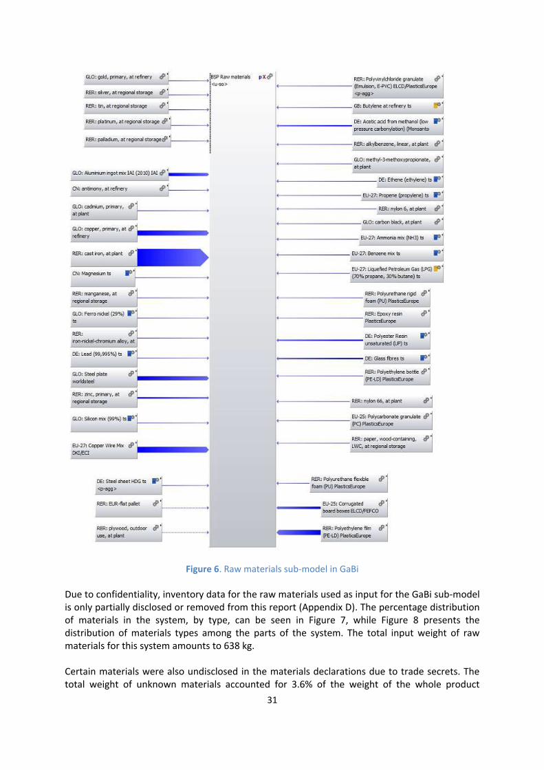
31

Figure 6. Raw materials sub-model in GaBi

Due to confidentiality, inventory data for the raw materials used as input for the GaBi sub-model is only partially disclosed or removed from this report (Appendix D). The percentage distribution of materials in the system, by type, can be seen in Figure 7, while Figure 8 presents the distribution of materials types among the parts of the system. The total input weight of raw materials for this system amounts to 638 kg. Certain materials were also undisclosed in the materials declarations due to trade secrets. The total weight of unknown materials accounted for 3.6% of the weight of the whole product

32

system and was allocated among the known materials considered in the sub-model by preserving the same ratio of their weights. Almost half of the unknown materials in the system come from cabling, and 1/3 comes from the processor boards. Possible implications of these data gaps and the adopted simplification are discussed in Chapter 7. The materials declaration for the active patch panel, which forms part of the BSP system, was impossible to obtain during this study. However, many of its components and the materials comprising them have been identified in the materials declaration of the cabinet, so it is assumed that the patch panel is accounted for in the data on the cabinet level.

Figure 7. Percentage distribution of raw materials by type, including packaging

Figure 8. Distribution of raw materials by type per group of parts

Packaging in figures 7 and 8 refers to all packaging used during the life cycle including the packaging for the final delivery of the product, but excluding any packaging that might be used for raw materials during processing and transportation to suppliers. The packaging models are discussed further in Section 4.4.2.3 below.

4.4.2.2 Inventory data on cabling

Although the above BSP system includes cabling, data on cables used in BSP 8100, the materials they contain and their weights has been collected from different sources. First, all cable products that can be used in a BSP 8100 configuration have been identified through hardware description documents (Ericsson, 2012c). Due to the inaccessibility of the materials declarations, cabling raw

48%

12%

6%

31%

3%

Metals

Plastics

Other

Wood

Paper

0% 5% 10% 15% 20% 25% 30% 35% 40% 45% 50%

Boards

Subracks

Cabinet

PFM

Cables

Packaging

Metals Plastics Other Wood Paper

33

materials were taken from the parallel LCA study on RBS (Ericsson, 2016e) where raw materials content depends on three cable types: power, signal and coaxial. The data contained the mass of every material per kilogram of cable. The same raw materials grouping approach described in Section 4.4.2.1 has been used for the raw materials of cabling. As documentation on the weights of cable products was inaccessible, some cable sets used in BSP 8100 and available in an Ericsson test lab have been measured to fill in the data gaps. Only 7 out of 19 cable products used in BSP were available for measuring. Other cable products that are not used in BSP, but were available, have also been measured to obtain data on the mass of different cable products for better assumptions. Cable products come in different lengths and from the obtained measurements, the mass of 1 m of cable (or 0,1 m for shorter cables) per product type was calculated. Assumptions on the mass of the unmeasured cable products were based depending on their products number, use and cable type. A cabling scenario representing an average case of cabling for a BSP configuration has been used to perform the calculations and obtain the input data used for GaBi modelling. A more conservative cabling scenario covering more extensive cabling (with two patch panels which allow for optical connection) has been considered. It affects the use of cable sets considerably, and it poses the requirements of more cabling in a configuration. A Capturing Unit functionality is also included in the cabling scenario. For cable products where a range of various cable lengths are available, the medium cable length has been assumed for the purposes of this study. For example, if a cable product is available in 10 m, 30 m and 60 m variants, the 30 m variant is chosen for the calculations in this study. The reason is that BSP 8100 as core network equipment is usually placed in data centres where connections to other equipment or to the electricity grid often require long cabling. This approach has been considered representative of a realistic scenario by experts within Ericsson. After all measurements and assumptions of cable weights and lengths have been made, calculations about the total weights of coaxial, power and signal cables have been perfomed. From there, the weights of all cabling raw materials have been defined and added to the general values for raw materials weight used as parameters in the GaBi sub-model presented in Figure 6.

4.4.2.3 Inventory data on packaging

The packaging considered in this study includes the packaging of the BSP 8100 system as the final product delivered to customers and the packaging of the different intermediate products delivered from suppliers to the final assembly site. The data on packaging has been collected from different sources, and the acquisition processes for packaging materials are based on secondary GaBi data. Data on the raw materials in the packaging of final products (equipped cabinet) and their corresponding weights have been collected from the products’ materials declarations and from internal Ericsson documents on packaging (such as Ericsson, 2015d; 2015e). In the modelled packaging scenario, the studied cabinet is considered a new sale, i.e. the final product is delivered to customers fully equipped and involves packaging for the cabinet and separate packaging for all the processor blades, but does not include packaging for subracks and cables.

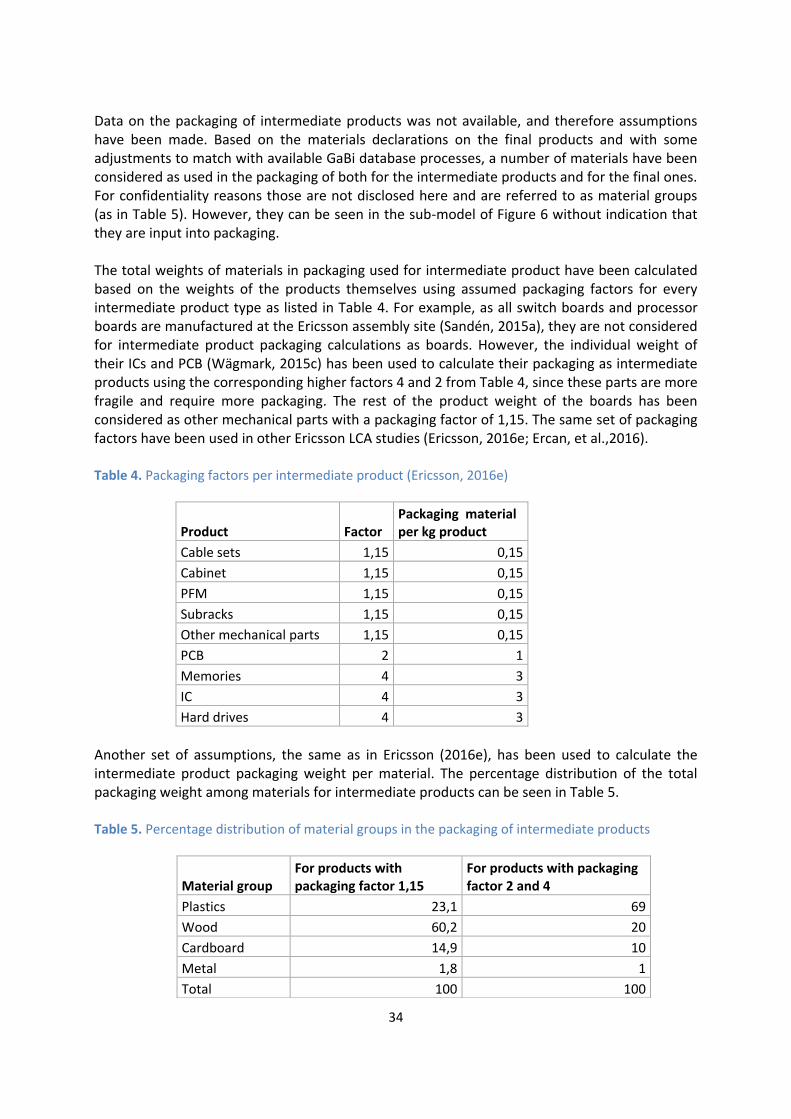
34

Data on the packaging of intermediate products was not available, and therefore assumptions have been made. Based on the materials declarations on the final products and with some adjustments to match with available GaBi database processes, a number of materials have been considered as used in the packaging of both for the intermediate products and for the final ones. For confidentiality reasons those are not disclosed here and are referred to as material groups (as in Table 5). However, they can be seen in the sub-model of Figure 6 without indication that they are input into packaging. The total weights of materials in packaging used for intermediate product have been calculated based on the weights of the products themselves using assumed packaging factors for every intermediate product type as listed in Table 4. For example, as all switch boards and processor boards are manufactured at the Ericsson assembly site (Sandén, 2015a), they are not considered for intermediate product packaging calculations as boards. However, the individual weight of their ICs and PCB (Wägmark, 2015c) has been used to calculate their packaging as intermediate products using the corresponding higher factors 4 and 2 from Table 4, since these parts are more fragile and require more packaging. The rest of the product weight of the boards has been considered as other mechanical parts with a packaging factor of 1,15. The same set of packaging factors have been used in other Ericsson LCA studies (Ericsson, 2016e; Ercan, et al.,2016). Table 4. Packaging factors per intermediate product (Ericsson, 2016e)

Product Factor Packaging material per kg product

Cable sets 1,15 0,15

Cabinet 1,15 0,15

PFM 1,15 0,15

Subracks 1,15 0,15

Other mechanical parts 1,15 0,15

PCB 2 1

Memories 4 3

IC 4 3

Hard drives 4 3

Another set of assumptions, the same as in Ericsson (2016e), has been used to calculate the intermediate product packaging weight per material. The percentage distribution of the total packaging weight among materials for intermediate products can be seen in Table 5. Table 5. Percentage distribution of material groups in the packaging of intermediate products

Material group For products with packaging factor 1,15

For products with packaging factor 2 and 4

Plastics 23,1 69

Wood 60,2 20

Cardboard 14,9 10

Metal 1,8 1

Total 100 100

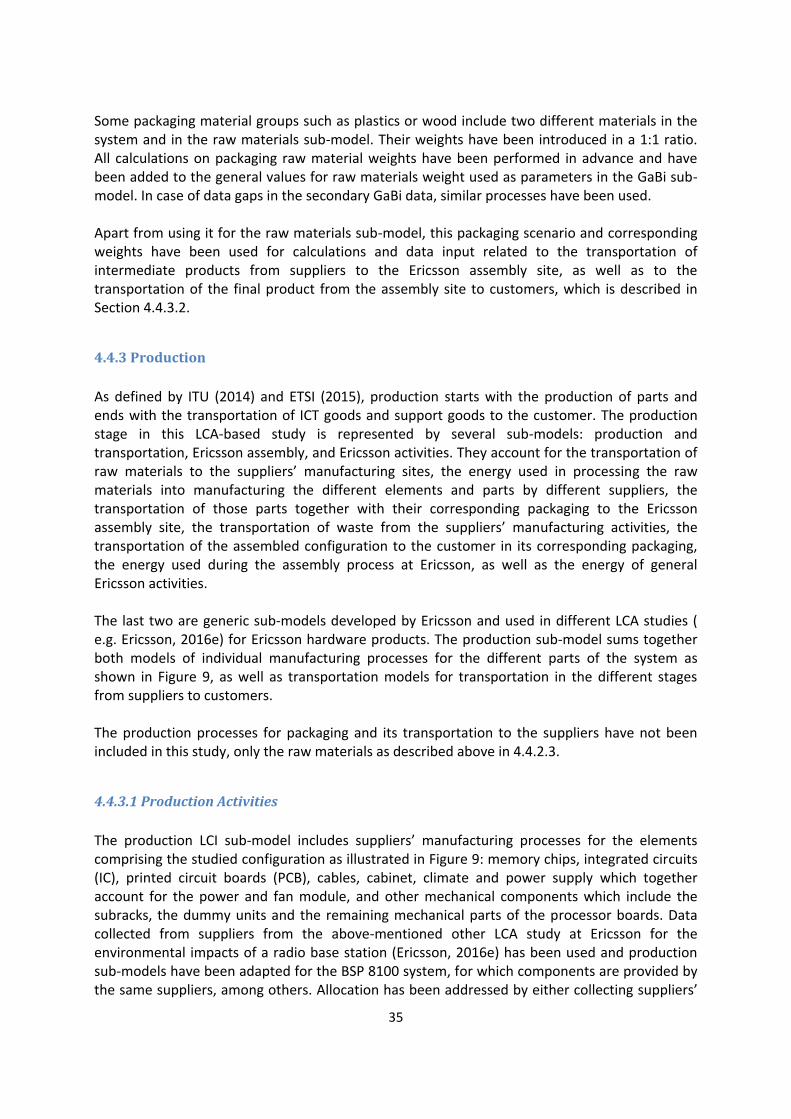
35

Some packaging material groups such as plastics or wood include two different materials in the system and in the raw materials sub-model. Their weights have been introduced in a 1:1 ratio. All calculations on packaging raw material weights have been performed in advance and have been added to the general values for raw materials weight used as parameters in the GaBi sub-model. In case of data gaps in the secondary GaBi data, similar processes have been used. Apart from using it for the raw materials sub-model, this packaging scenario and corresponding weights have been used for calculations and data input related to the transportation of intermediate products from suppliers to the Ericsson assembly site, as well as to the transportation of the final product from the assembly site to customers, which is described in Section 4.4.3.2.

4.4.3 Production

As defined by ITU (2014) and ETSI (2015), production starts with the production of parts and ends with the transportation of ICT goods and support goods to the customer. The production stage in this LCA-based study is represented by several sub-models: production and transportation, Ericsson assembly, and Ericsson activities. They account for the transportation of raw materials to the suppliers’ manufacturing sites, the energy used in processing the raw materials into manufacturing the different elements and parts by different suppliers, the transportation of those parts together with their corresponding packaging to the Ericsson assembly site, the transportation of waste from the suppliers’ manufacturing activities, the transportation of the assembled configuration to the customer in its corresponding packaging, the energy used during the assembly process at Ericsson, as well as the energy of general Ericsson activities. The last two are generic sub-models developed by Ericsson and used in different LCA studies ( e.g. Ericsson, 2016e) for Ericsson hardware products. The production sub-model sums together both models of individual manufacturing processes for the different parts of the system as shown in Figure 9, as well as transportation models for transportation in the different stages from suppliers to customers. The production processes for packaging and its transportation to the suppliers have not been included in this study, only the raw materials as described above in 4.4.2.3.

4.4.3.1 Production Activities

The production LCI sub-model includes suppliers’ manufacturing processes for the elements comprising the studied configuration as illustrated in Figure 9: memory chips, integrated circuits (IC), printed circuit boards (PCB), cables, cabinet, climate and power supply which together account for the power and fan module, and other mechanical components which include the subracks, the dummy units and the remaining mechanical parts of the processor boards. Data collected from suppliers from the above-mentioned other LCA study at Ericsson for the environmental impacts of a radio base station (Ericsson, 2016e) has been used and production sub-models have been adapted for the BSP 8100 system, for which components are provided by the same suppliers, among others. Allocation has been addressed by either collecting suppliers’

36

production data that is only related to Ericsson intermediate products or, which is more often the case, by obtaining yearly data together with data on the Ericsson share of their production to allocate by volume. All the data is processed to obtain values which are relevant for one unit mass of hardware (or one unit surface area for ICs, memories or PCBs). Generic GaBi database processes for electricity, waste treatment when known, etc. have been used together with the Ericsson production data to model the production of the different parts (see Appendix B). Energy recovery has been accounted for where relevant. Necessary calculations have been performed in advance before the input of inventory data into the GaBi software. As mentioned above, the production and transportation of packaging prior its use by the suppliers is not part of this study due to data unavailability and time limitations.

Figure 9. Production sub-model with components models

According to Sandén (2015a, 2015b), the production of the printed board assemblies (PBA) and the process boards in general takes place in Poland. The manufacturing of PCB for them, however, takes place with suppliers elsewhere. The location in Poland is also the assembly site where cabinets are equipped and all BSP 8100 configurations assembled before being delivered to customers. Ericsson has a global supply chain with multiple suppliers for the same product. However, for the scenario modelled under this study a supplier of PCB located in China is chosen. From there PCBs are transported to Poland for the PBA assembly. ITU (2014) and ETSI (2015) define a mandatory set of parts to be included in the LCA. For example, integrated circuits, including memories, should be a mandatory part of every LCA study of ICT equipment and chip area is a possible product flow unit. From the mandatory set of parts and assembly unit processes this study does not include small components (such as resistors and

37

capacitors), batteries and electro-mechanics because of the lack of data. Furthermore, differentiation between different types of integrated circuits except for memories did not take place, and production processes for PBA components apart from PCB and the ICs were not included due to time restrictions. According to Ericsson experts, the omitted production processes are used to giving a limited contribution to the overall results. However, no quantitative cut-off analysis was performed. The production of cables is assumed to take place entirely in China. Although some of the cables used by Ericsson are known to be manufactured in Europe, and some even in Poland, which could possibly reduce impact from transportation and electricity use, due to the unavailability of accurate data for the purpose of this study, a more conservative approach has been adopted. Subracks are known to be mostly manufactured in Estonia, but for the lack of specific data on subracks production, data available for other mechanical parts has been also adopted for them. As data from the manufacturing processes of the BSP 8100 power and fan module was also unavailable, the data on the climate and power supply units from the RBS LCA study (Ericsson, 2016e) was adapted for the purpose of this case. The exact manufacturing locations considered for all the elements in this manufacturing scenario can be seen in Table 6. a) Memories The model for the production of memory chips is built using the total area of memory chips as a parameter in the GaBi software. It accounts for the energy use for the production of every unit area of the memories. The required data on the dimensions and weight of the memories and on their number on every PBA has been obtained from internal Ericsson sources (Wägmark, 2015c). Data gaps were filled by information acquired through dismantling a processor board and measuring the chip area. All calculations have been performed prior to entering data into GaBi. Based on knowledge within Ericsson and measurements performed on larger integrated circuits it is assumed that the chip area is 50% of the visible area of the plastic chip cover. The memories production model is built on the basis of suppliers’ data on memories production from the parallel RBS study (Ericsson, 2016e) and accounts for the energy input for the production of a total area of memories in square meters. The memories area is introduced by using a parameter in GaBi. Detailed data on memories cannot be disclosed due to confidentiality. However, calculating the memories area for all the processor boards comprising the system depending on board model has amounted to a total input of approximately 0,1 m2 of memories area. The memory model does not consider production waste treatment processes due to the lack of data from suppliers. b) Other integrated circuits Modelling and data collection for other integrated circuits has been performed in the same way as described above for memories. According to provided suppliers’ data, however, the model accounts not only for the energy input, but also for the processing of waste through waste disposal. The model is scaled up by chip area, and calculations based on all data collected estimate a total input of 0,06 m2 of integrated circuits in the studied system.

38

c) Printed circuit boards The modelling for the PCB production is scaled on the basis of surface area and is based on data from two different suppliers collected for Ericsson (2016e), one accounting only for the energy input in the system, while the other also accounts for the waste generated in the process and the energy recovered from it. There is an equal distribution of the manufactured PCBs among the two. The combined model is representing a square metre of produced PCB averaging between the two suppliers. The total PCB area in the system is introduced by using a parameter in GaBi. Data for the dimensions of the PCBs is obtained through Wägmark (2015c). After processing the available data calculations resulted in a total of 2,57 m2 of PCB in the studied system. d) Cables The cable production model is scaled by weight and is based on information provided by suppliers for the internal RBS study (Ericsson, 2016e). It accounts for the energy input in the production process through electricity and district heating, as well as for the waste disposal and energy recovery from the incineration of production waste for each unit weight of cabling. The weight of cables is introduced as a parameter, as in the above models. As stated in Table 1, a total weight of 82 kg is considered as part of the system. e) Cabinet The cabinet production model is scaled by weight and includes the energy input through the electricity used in the manufacturing phase and the disposal of hazardous waste such as paint and used mineral oil for a unit cabinet weight. The model is built based on the data provided by a supplier of indoors cabinets for the RBS study (Ericsson, 2016e), as cabinets used for BSP are only located indoors. The weight is introduced through a parameter and is calculated to be 75,4 kg based on data from the materials declaration. f) Climate part of the power and fan module Data and its corresponding model for the climate unit of the RBS study (Ericsson, 2016e) has been adapted scaled by weight to serve the climate part production in BSP 8100 due to the unavailability of primary data. The model accounts for energy input through electricity use for manufacturing and waste processing in terms of hazardous waste incineration per kilogram of climate part weight. The weight is introduced through the parameter function. An assumption for the weight of the climate part of the power and fan module has been estimated through data available in materials declarations and it amounts to 1,95 kg. g) Power supply part of the power and fan module The power supply part of the power and fan module production model is also based on data provided by suppliers for the RBS LCA study (Ericsson, 2016e) which is scaled by weight. The model includes the electricity used in the process, as well as waste treatment processes disposal of hazardous waste and landfilling of plastic waste per kilogram of power supply part weight. The weight is introduced through the parameter function. An assumption for the weight of the power supply part of the module has been estimated, as in the above case, through data

39

available in materials declarations and it amounts to 29,25 kg (there are six power and fan module units). h) Other mechanical parts Other mechanical parts in this study include the mechanical parts of the used boards in the system, the mechanical part of the active patch panel and the subracks. The data and model are scaled by weight from the ones of the RBS study (Ericsson, 2016e). The model accounts for the energy input through the use of electricity, diesel and natural gas and for the waste treatment through landfilling of solid municipal waste and disposal of hazardous waste per kilogram of other mechanical parts weight. Calculations based on data from the materials declarations estimate the weight to be 66,5 kg.

4.4.3.2 Transportation

In the LCI phase, the transportation sub-model has been designed to represent the three steps in the transportation activities relevant to the production of the system and its delivery to customers: transportation to the assembly site (including transportation of raw materials, waste and components before assembly), transportation from the assembly site to Sweden where all BSP 8100 configurations are shipped to, and transportation from Sweden to customers globally. Transportation during raw materials extraction is included to an unknown extent in the used secondary GaBi data and forms part of the raw materials acquisition stage. The transportation models are based on database processes from the GaBi software (listed in Appendix B) and account for the fuels used. These models built for the three stages of the transportation activities are structured identically, as shown in Figure 10, and represent a combination of air transport, sea transport and road transport consisting both of lorry transport and small lorry (7.5t) transport. However, different inventory data is used and calculations have been performed in advance to scale the corresponding payload distances. a) Production transports The production transport model is based on a scenario where all parts except for the power and fan module (both climate and power supply units) are manufactured in different locations and transported to the assembly site by air. The power and fan module is transported by sea. The assembly site is in Poland. Transportation to and from the corresponding airports and ports takes place by road. The scenario is based mostly on Sandén (2015a, 2015b) and involves certain assumptions presented below.

40

Figure 10. Generic transportation model used for every transportation stage

The suppliers for this scenario were selected randomly depending on the availability of data from the internal LCA study on a radio base station (Ericsson, 2016e), and the manufacturing locations were chosen either based on the data they provided or on information available on their websites. The scenario includes the manufacturing locations and the corresponding data on distances and product weights from Table 6. Road distances have been calculated taking into account the exact addresses of the suppliers. The names of the suppliers as well as all the data they have provided remain confidential. Table 6. Manufacturing locations per component and corresponding distances and weights used for calculating input LCI data

Product Manufacturing location

Road distance to airport/port (km)

Sea distance (km)

Air distance (km)

Total weight of product transported to assembly site, including packaging (kg)

PCB Hong Kong 50 0 8358 31,7

Cabinet Shenzhen, China 11 0 8323 86,7

Cables Shenzhen, China 50 0 8323 94,3

Power supply Jiangsu, China 128 21005 0 35,9

Climate unit Guangdong, China 1406* 0 0 2,2

ICs Taiwan 79,1 0 8566 24,1

Memory chips Gyeonggi-do, Korea 120 0 7733 2

Other mechanical parts

Jiangsu, China 32 0 7921 76,5

Note: * Road distance from climate unit supplier to power supply module supplier

41

Distances between the different locations were calculated through Google (2016), DistanceFromTo (2016), GlobeFeed.com (2015) and Sea-distances.org (2016). In Poland, the distance from the airport to the assembly site is considered 43 km, while the distance from the port to the site is 65 km (Google, 2016). Apart from the transports described above, the manufacturing transports sub-model contains data provided by the suppliers in reference to raw materials and production wastes (Ericsson, 2016e). Based on the data provided, calculations have been performed to obtain the payload-distance, in tkm, by road, sea and air for every kilogram of transported equipment by intermediate product type. The detailed data is confidential, but the results of the calculation providing the total payload-distances in tkm per product type as further input data for the GaBi model can be seen in Table 7. A sensitivity analysis has been performed about the total payload-distance for memory chips presented in Table 7, as the value seems unrealistically high, but no fault could be traced in the data. The results of the analysis are presented in Section 5.3.2. Table 7. Total payload-distances for other transports (raw materials and manufacturing waste)

Product type Total road, tkm Total air, tkm Total sea, tkm

PCB 127,8 0 0

Cabinet 43,45 0 0,375

Cables 47,30 0 0

PFM power supply 235,72 829 0

PFM climate 0,0015 0 0

ICs 3,92 0 0

Memories 3615 0 0

Other mechanical parts 26,96 0 0

TOTAL OTHER TRANSPORTS 4100,152 829 0,375

b) Transports from assembly site to Sweden According to Sandén (2015b), from the assembly site in Poland all BSP 8100 configurations are shipped to Sweden, 80% being transported to the Ericsson storage facilities in Gothenburg and the rest to the site in Borås. The scenario modelled involves that in Poland the studied configuration is transported by road from the assembly site in Poland to the port in Gdynia (65 km). After that it is sent by sea to the port of Karlskrona, Sweden, which covers a distance of 306 km. Later, 80% of the system is transported by truck to Gothenburg (355 km) and 20% by truck to Borås (280 km). To calculate the payload-distance for the modelling of this transportation phase a total load of 361.04 kg was considered. c) Transports from Sweden to customers The scenario for modelling the transportation phase from Sweden to the customers is based on confidential BSP 8100 delivery data provided by Sandén (2016). It discloses the number of BSP 8100 delivered per Ericsson sales region for a period of three months which serves as a foundation for allocation of deliveries for the functional unit. Assumptions for a possible delivery destination in every region were made, as presented in Table 8, in order to calculate distances

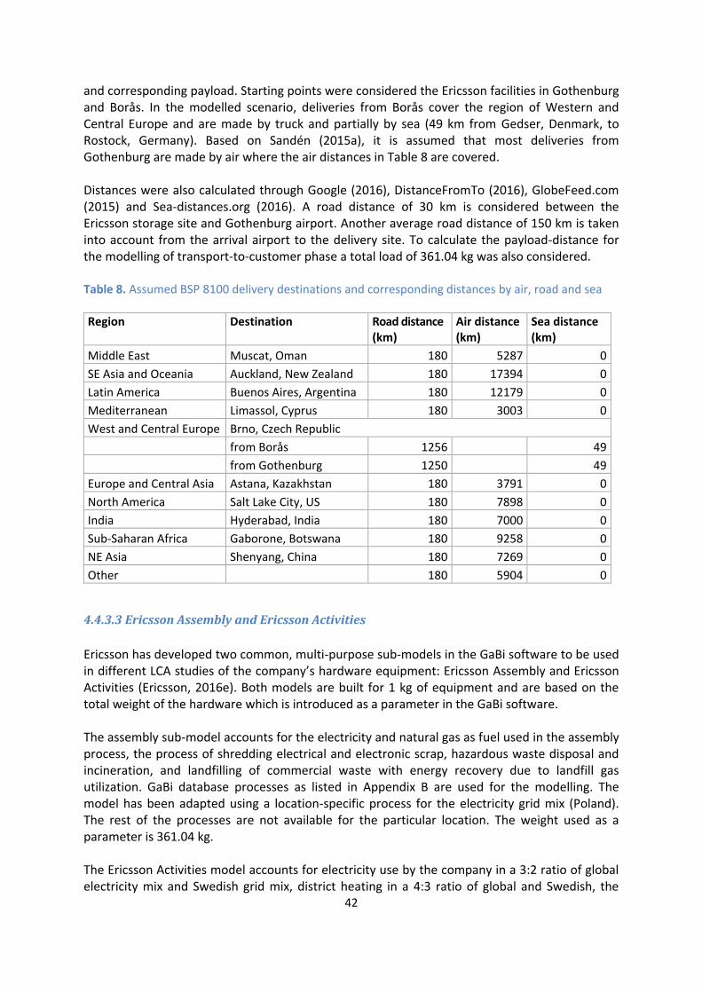
42

and corresponding payload. Starting points were considered the Ericsson facilities in Gothenburg and Borås. In the modelled scenario, deliveries from Borås cover the region of Western and Central Europe and are made by truck and partially by sea (49 km from Gedser, Denmark, to Rostock, Germany). Based on Sandén (2015a), it is assumed that most deliveries from Gothenburg are made by air where the air distances in Table 8 are covered. Distances were also calculated through Google (2016), DistanceFromTo (2016), GlobeFeed.com (2015) and Sea-distances.org (2016). A road distance of 30 km is considered between the Ericsson storage site and Gothenburg airport. Another average road distance of 150 km is taken into account from the arrival airport to the delivery site. To calculate the payload-distance for the modelling of transport-to-customer phase a total load of 361.04 kg was also considered. Table 8. Assumed BSP 8100 delivery destinations and corresponding distances by air, road and sea

Region Destination Road distance (km)

Air distance (km)

Sea distance (km)

Middle East Muscat, Oman 180 5287 0

SE Asia and Oceania Auckland, New Zealand 180 17394 0

Latin America Buenos Aires, Argentina 180 12179 0

Mediterranean Limassol, Cyprus 180 3003 0

West and Central Europe Brno, Czech Republic

from Borås 1256

49

from Gothenburg 1250

49

Europe and Central Asia Astana, Kazakhstan 180 3791 0

North America Salt Lake City, US 180 7898 0

India Hyderabad, India 180 7000 0

Sub-Saharan Africa Gaborone, Botswana 180 9258 0

NE Asia Shenyang, China 180 7269 0

Other

180 5904 0

4.4.3.3 Ericsson Assembly and Ericsson Activities

Ericsson has developed two common, multi-purpose sub-models in the GaBi software to be used in different LCA studies of the company’s hardware equipment: Ericsson Assembly and Ericsson Activities (Ericsson, 2016e). Both models are built for 1 kg of equipment and are based on the total weight of the hardware which is introduced as a parameter in the GaBi software. The assembly sub-model accounts for the electricity and natural gas as fuel used in the assembly process, the process of shredding electrical and electronic scrap, hazardous waste disposal and incineration, and landfilling of commercial waste with energy recovery due to landfill gas utilization. GaBi database processes as listed in Appendix B are used for the modelling. The model has been adapted using a location-specific process for the electricity grid mix (Poland). The rest of the processes are not available for the particular location. The weight used as a parameter is 361.04 kg. The Ericsson Activities model accounts for electricity use by the company in a 3:2 ratio of global electricity mix and Swedish grid mix, district heating in a 4:3 ratio of global and Swedish, the

43

electricity used for the outsourced IT services, passenger-distance of air travel, passenger-distance of road transport by car, and commuting also expressed through the passenger-distance by car, the production of the corresponding laptop computers used including the corresponding raw materials acquisition and the use of paper as office supply. The global electricity mix that Ericsson uses in relation to its activities and assembly is a mixture of European, Japanese, U.S. and Chinese electricity grid mixes in a ratio 10:5:3:2. The input data is confidential and hence undisclosed. The database processes from the GaBi software are listed in Appendix B.

4.4.4 Use

The sub-model of the use stage accounts for the electricity used to operate the system for a period of five years, including two leap years, or 1827 days. GaBi database processes have been used in this sub-model as well. The power consumption of the system has been calculated using data from the hardware description (Ericsson, 2016b). There has been an intention to build the use sub-model for a scenario of BSP 8100 deliveries based on the confidential Ericsson data from Sandén (2016). However, the lack of regional or local database processes on electricity mixes has prevented from building such a sub-model. Therefore, a simplified model reproducing the one for the Ericsson world average mix used in the sub-model for the Ericsson activities has been applied (European, Japanese, U.S. and Chinese electricity grid mixes in a ratio 10:5:3:2), and a sensitivity analysis has been performed on it (see Section 5.3.3). The power consumption value used in the use scenario cannot be disclosed due to a confidentiality agreement, but it accounts for the average consumption of all of the parts of the system.

4.4.5 End-of-life Treatment

Experts at Ericsson recommended that the end-of-life treatment (EoLT) stage be based on a scenario where the system is mostly recycled under the assumption that it represents business-to-business equipment and there is control over the life cycle, including its EoL stage. Due to the unavailability of data on the EoLT of BSP 8100 the model was reused an LCA study on a smartphone (Ercan, et al., 2016). It is based on Liebmann (2015) where regional waste flows were investigated and results were aggregated to create a global scenario for the EoLT of ICT equipment. The model built by Ercan, et al. (2016) is based on Liebmann’s global scenario where 83% of the mass of the equipment is recycled and 17% is landfilled. Although Liebmann (2015) shows that informal recycling constitutes 64% of the total ICT waste versus 19% of formal recycling, these figures mostly concern end-user equipment. Network equipment is mostly formally recycled or reused, although cases of informal recycling have also been reported (Liebmann, 2015). Therefore, the above 83% vs. 17% scenario is adopted for this LCA study accounting for 83% of the mass of the final product. The data on the recycling process is based on the recycling sites of two companies, while GaBi generic data is used for landfill processes. As in Ercan, et al. (2016) modelling transports associated with recycling follows Ericsson’s internal conditions for recycling. The preparation for reuse is not accounted for in this study.

44

The model from Ercan, et al. (2016) was adapted for BSP 8100 (see Figure 11), and it accounts for the energy use for recycling of the system which is covered by the Ericsson global electricity mix presented in Section 4.4.4, natural gas, diesel mix and heavy fuel oil and for transportation by truck. The scenario also includes landfilling of 0,017 kg of plastics and 0,153 kg of ferro metals for every kilogram of product. The input of the product mass undergoing EoLT into the sub-model has been completed using the parameter function. The EoLT of packaging is outside the system and is not accounted for in this sub-model. The EoLT model includes only the EoLT process and avoided burdens are not accounted for. As mentioned in 5.4.2, they are accounted for to an unknown extent in the data embedded in the GaBi database processes used in modelling the raw materials acquisition stage.

Figure 11. EoL treatment model

4.5 Allocation In the raw materials acquisition stage allocation has been avoided by collecting data on the raw materials input in the system from the products’ materials declarations where the content of each material is available by mass (see 4.4.2 for more details on raw materials acquisition inventory data). For every modelled material, acquisition processes from the GaBi databases have been used. This required calculations to allocate some materials among different database processes due to the unavailability of a database processes covering solely that material. The only such case in the studied system concerns the acquisition of chromium (Cr) and nickel (Ni) and also affects the modelled acquisition of iron (Fe). Physical allocation by mass has been performed in this case. As acquisition of chromium in the GaBi datasets is available only in the process of acquiring “iron-nickel-chromium alloy” with ratio 23:30:47 according to the documentation in GaBi (PE

45

International, 2016), the input mass of that alloy in the system has been calculated based on the required amount of chromium. The acquisition of this alloy covers certain amounts of the nickel and iron required in the system. After that, the remaining amount of nickel needed has been covered by another GaBi process “Ferro nickel” acquiring 29% of Ni and 71% Fe according to the GaBi documentation (PE International, 2016). The rest of the iron has been allocated to a GaBi process for cast iron. All the three Gabi processes are listed in Appendix B. The production of intermediate products for Ericsson is done by multiple suppliers who supply other companies with products manufactured on their site, and therefore allocation cannot be avoided. For the production stage, allocation is addressed after the rules for facility data according to ETSI (2015, p.50) and is based on relevant physical data – mass or surface area. Data about the production activities from suppliers has been collected by other researchers under the internal Ericsson study on the potential environmental impacts of a radio base station (Ericsson, 2016e). Suppliers manufacturing different parts/intermediate products of the product systems (cabinets, PCB, memories, other integrated circuits, cables, etc.) as presented in 4.4.3 have been contacted. Production sites are specialized in manufacturing a particular intermediate product and therefore a physical approach to partitioning is considered the most adequate. Suppliers have been asked to provide data on production processes, involved energy input, transportation (of raw materials, waste or other) and production waste treatment corresponding only to the intermediate products manufactured for Ericsson from a particular production site in one year. Then, through calculations data is obtained for every kilogram (or square metre in the case of IC and PCB) of product produced. The production is modelled for 1 kg (or 1 m2) of intermediate product and is scaled by the corresponding total weight of that product within the studied system expressed as a parameter in GaBi. If suppliers cannot provide data specifically on the Ericsson share of the production, they provide yearly data on the whole production site and data on what share of the yearly production is for Ericsson. This quantity is expressed in comparable units – usually per kilogram of equipment or per surface area in the case of integrated circuits and PCB. Even if data on IC and PCB is given for a certain weight of products, details available in the product descriptions allow for accurate conversion to the necessary units. With a series of calculations, all flows and processes for every kilogram weight (or square metre surface area where relevant) of equipment are quantified. The GaBi models are built based on a kilogram weight of every type of intermediate product or square metre of surface area in the case of chips and PCB. Then the corresponding weight of that intermediate product in the studied product system is introduced as a parameter in GaBi to obtain results from the modelled activities for the studied product system. When data on the production of an intermediate product is available from more than one supplier, such as the case of PCB described in 4.4.3.1 c), it is modelled by building individual sub-models following the data on processes and flows provided by each supplier. The contribution of every sub-model to the entire production model for that particular part is assigned by a factor or introduced as a parameter in the GaBi software, taking into account the share of each supplier when contributing to the yearly supply of this particular part, expressed in units of mass or surface area. In the case of Ericsson, assembly sites assemble different products which belong to different products systems. Assembly sites may also be run by a third party and provide assembling services to other companies. Therefore, allocation when accounting for the contribution of the assembly process and facility to the environmental impacts of the studied system cannot be

46

avoided. The data on Ericsson Assembly activities also counts as facility data for production facilities as defined by ETSI (2015) and therefore is allocated based on relevant physical data. Partitioning the input and output data for the Ericsson Assembly model described in 4.4.3.3 has been done by other researchers for the RBS study by Ericsson (Ericsson, 2016e) by collecting yearly data from the whole assembly site and accounting for the total number of equipped cabinets (by number of units) assembled on that site in one year. As configurations differ, further allocation is done by mass based on the average weight of one cabinet to obtain quantifications for all the energy and assembly processes corresponding to 1 kilogram of assembled equipment (i.e. the allocation key). The GaBi model is built for 1 kilogram of assembled equipment and is scaled by the weight of the corresponding product system (i.e. configuration of equipped cabinet), in this case the BSP system from Table 1. A similar physical approach is used to partition data and model Ericsson Activities also described in 4.4.3.3 for an allocation key of 1 kilogram of produced hardware by the company. It accounts for support activities between different projects/products according to ETSI (2015, p. 50) and is allocated to the production stage. The model is based only on data about produced cabinets and not on other types of hardware by Ericsson. Data is collected about the energy, manpower, their travel, equipment and paper used by employees for one year and allocation is done per cabinet based on the total number of cabinets sold that year. Then this is divided by the average weight of a cabinet to obtain data per one kilogram of cabinet and built the GaBi model on it. According to ETSI (2015, p. 50), “*t+ransports should be allocated based on chargeable mass or volume whichever limits the transport capacity.” In this study, as described in 4.4.3.2 allocation during the production stage for transport activities with suppliers (associated with the delivery of raw materials and with the treatment of production waste), from suppliers to the assembly site and from the assembly site to the hubs in Sweden has been done by mass based on 1 kilogram of product. Different parts of the system undergo transportation by road, air and sea in different stages and cover different distances, and these have been duly partitioned. Also, a global delivery scenario has been accounted where the product system is to be delivered from the hubs in Sweden in locations in different sales regions. There, physical allocation has been done based on sales volumes to partition the data. Empty return trips are not considered applicable in this study. No allocation procedure has been performed to model the use stage which only accounts for the electricity used to operate the system. Allocation has been avoided by increasing the level of detail and obtaining the overall electricity consumption of the system by gathering data on the electricity consumption of the different parts of that system. Any allocation among co-products in electricity production is accounted for in the GaBi datasets. As pointed in the ISO 14040 (ISO, 2006a), the need for allocation procedures has to be considered when dealing with multiple recycling systems too. In the case of the studied product system, no data has been accessible on the EoL stage and the recycling of materials of the system in the deployment locations. Therefore, in order to avoid allocation of recovered materials based on unsubstantiated assumptions, a simplified, more conservative EoLT scenario (as described and motivated in 4.4.5) was assumed where recycling is accounted for only as a process in terms of transportation and energy input based on data from recycling companies given to Ercan, et al. (2016). Average data on recycling has been collected based on 1 kg of plastics and 1 kg of metals with an average rate of 83% recycling rate. For the landfill processes secondary GaBi data has been used.

47

5. Results from the Life Cycle Impact Assessment (LCIA) and

Interpretation This chapter presents the results for the potential environmental impacts obtained under the this study and their interpretation. It introduces the LCIA which aims to present the environmental consequences from the environmental loads quantified in the LCI (Baumann and Tillman, 2004). When using “ready-made” LCIA methods, as in this study, many of the sub-phases described in Section 2.3 “are not executed by the LCIA practitioner, since they are “inside” the LCIA method” (Baumann and Tillman, 2004, p. 135). The impact categories, category indicators and characterisation models selected for this study are based on the ILCD recommendations. They have been made by the Joint Research Centre – Institute of Environment and Sustainability with the European Commission after the evaluation of different characterisation methods for every impact category in a European context, and are currently applied by Ericsson for LCA. These are so-called midpoint characterisation methods which provide indicators to compare environmental interventions at a midpoint level of the cause-effect chain, i.e. between emissions or resource consumption and the endpoint level (where a damage approach would be applied). (European Union, 2011) Although results are shown for all impact categories, this study places greater focus on climate change.

5.1 Overall Results As Figure 12 shows, the raw materials stage has the highest contribution in the impact categories of freshwater eutrophication, freshwater ecotoxicity and abiotic resource depletion holding correspondingly 99%, 95% and 95% of the total impact in these categories. It also has significant human toxicity potential (non-cancer effects 88%, cancer effects 46%), and holds almost half of the ozone depletion potential. In addition, this life cycle stage accounts for 21% of the total marine eutrophication of the system and 12% of the acidification potential. The production stage, which includes production activities, transports and Ericsson assembly and activities as described in Section 4.4.3, dominates in the water depletion impact category by 87%. It also contributes to about 32% of the ozone depletion potential of the system and to about 19% of its potential impact on terrestrial eutrophication. It also accounts for 17% of the photochemical ozone formation, for 13% of the total marine eutrophication and ionizing radiation potentials, and for 12% in the acidification and particulate matter impact categories. The use stage which accounts for the electricity consumed throughout the operation of the system dominates in a number of impact categories: acidification (76%), climate change and climate change with biogenic carbon (92%), marine (65%) and terrestrial (74%) eutrophication, ionising radiation (70%), particulate matter (81%) and photochemical ozone formation (76%). It also contributes to approximately half of the impact potential of human toxicity with cancer effects, to 20% of the ozone depletion potential and to 11% of both water depletion and human toxicity with non-cancer effects.

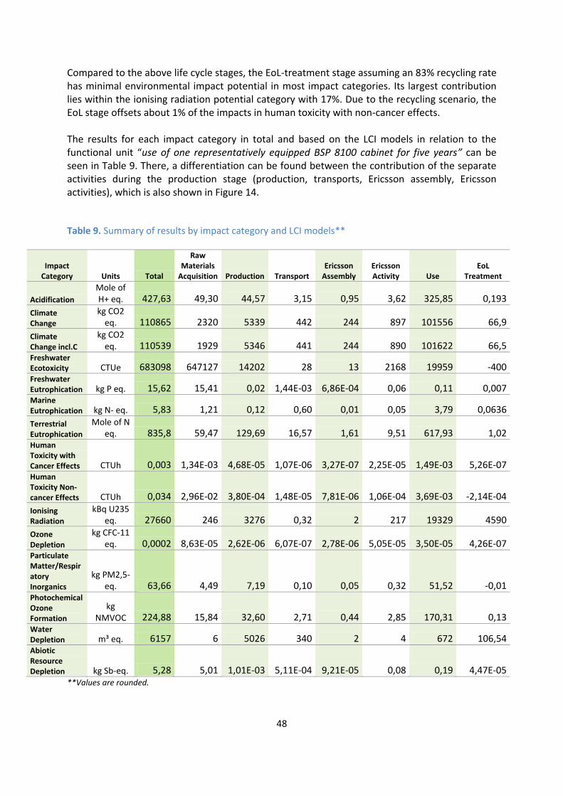
48

Compared to the above life cycle stages, the EoL-treatment stage assuming an 83% recycling rate has minimal environmental impact potential in most impact categories. Its largest contribution lies within the ionising radiation potential category with 17%. Due to the recycling scenario, the EoL stage offsets about 1% of the impacts in human toxicity with non-cancer effects. The results for each impact category in total and based on the LCI models in relation to the functional unit “use of one representatively equipped BSP 8100 cabinet for five years” can be seen in Table 9. There, a differentiation can be found between the contribution of the separate activities during the production stage (production, transports, Ericsson assembly, Ericsson activities), which is also shown in Figure 14.

Table 9. Summary of results by impact category and LCI models**

Impact Category Units Total

Raw Materials

Acquisition Production Transport Ericsson

Assembly Ericsson Activity Use

EoL Treatment

Acidification

Mole of H+ eq. 427,63 49,30 44,57 3,15 0,95 3,62 325,85 0,193

Climate Change

kg CO2 eq. 110865 2320 5339 442 244 897 101556 66,9

Climate Change incl.C

kg CO2 eq. 110539 1929 5346 441 244 890 101622 66,5

Freshwater Ecotoxicity CTUe 683098 647127 14202 28 13 2168 19959 -400 Freshwater Eutrophication kg P eq. 15,62 15,41 0,02 1,44E-03 6,86E-04 0,06 0,11 0,007 Marine Eutrophication kg N- eq. 5,83 1,21 0,12 0,60 0,01 0,05 3,79 0,0636

Terrestrial Eutrophication

Mole of N eq. 835,8 59,47 129,69 16,57 1,61 9,51 617,93 1,02

Human Toxicity with Cancer Effects CTUh 0,003 1,34E-03 4,68E-05 1,07E-06 3,27E-07 2,25E-05 1,49E-03 5,26E-07 Human Toxicity Non-cancer Effects CTUh 0,034 2,96E-02 3,80E-04 1,48E-05 7,81E-06 1,06E-04 3,69E-03 -2,14E-04

Ionising Radiation

kBq U235 eq. 27660 246 3276 0,32 2 217 19329 4590

Ozone Depletion

kg CFC-11 eq. 0,0002 8,63E-05 2,62E-06 6,07E-07 2,78E-06 5,05E-05 3,50E-05 4,26E-07

Particulate Matter/Respiratory Inorganics

kg PM2,5-eq. 63,66 4,49 7,19 0,10 0,05 0,32 51,52 -0,01

Photochemical Ozone Formation

kg NMVOC 224,88 15,84 32,60 2,71 0,44 2,85 170,31 0,13

Water Depletion m³ eq. 6157 6 5026 340 2 4 672 106,54 Abiotic Resource Depletion kg Sb-eq. 5,28 5,01 1,01E-03 5,11E-04 9,21E-05 0,08 0,19 4,47E-05

**Values are rounded.

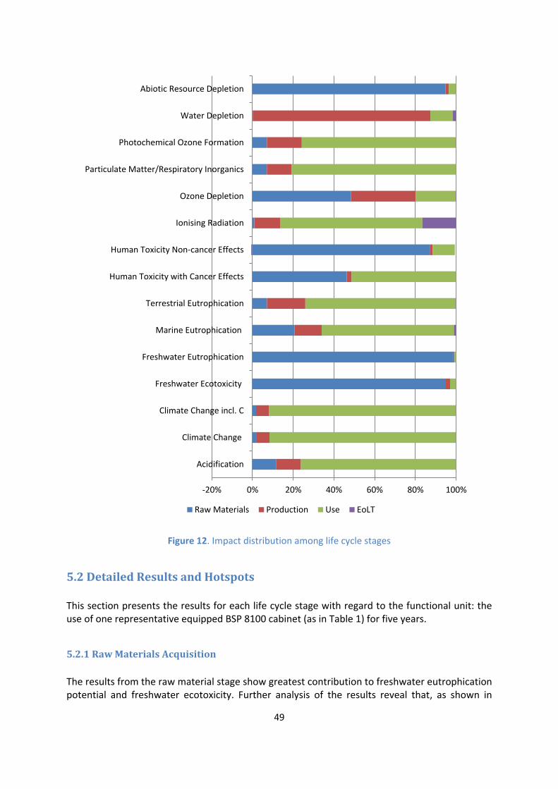
49

Figure 12. Impact distribution among life cycle stages

5.2 Detailed Results and Hotspots This section presents the results for each life cycle stage with regard to the functional unit: the use of one representative equipped BSP 8100 cabinet (as in Table 1) for five years.

5.2.1 Raw Materials Acquisition

The results from the raw material stage show greatest contribution to freshwater eutrophication potential and freshwater ecotoxicity. Further analysis of the results reveal that, as shown in

-20% 0% 20% 40% 60% 80% 100%

Acidification

Climate Change

Climate Change incl. C

Freshwater Ecotoxicity

Freshwater Eutrophication

Marine Eutrophication


Human Toxicity with Cancer Effects

Human Toxicity Non-cancer Effects

Ionising Radiation

Ozone Depletion



Water Depletion

Abiotic Resource Depletion

Raw Materials Production Use EoLT

50

Figure 13, the main contribution to freshwater eutrophication comes from the acquisition of gold (7,96 kg P eq.) and copper (6,57 kg P eq.). Again gold (323454 CTUe) and copper (288846 CTUe) are the main causes for the freshwater ecotoxicity potential. They also contribute mostly to human toxicity with non-cancer effects. The acquisition of silver contributes to 54% of the total abiotic resource depletion potential of the raw materials phase, as illustrated in Figure 13, followed by gold contributing by 18% and antimony with 17%. The rest of the most contributing materials under all impact categories can also be seen in Figure 13. The results from this life cycle stage are in line with the findings from an LCA of metal production system conducted by Nuss and Eckelman (2014).

Figure 13. Contribution of different materials in the raw materials acquisition stage

5.2.2 Production

This section summarizes the results of the production life cycle stage as presented in the LCI sub-model in Section 4.4.3. In general terms, the biggest contribution comes from the production activities, while the smallest contribution comes from the assembly.

-20% 0% 20% 40% 60% 80% 100%

Acidification

Climate Change








Ionising Radiation

Ozone Depletion



Water Depletion


Gold (Au) Copper (Cu) Silver (Ag) Antimony (Sb) Tin (Sn)

Aluminium (Al) Cast iron Plywood Rest

51

As shown in Figure 14 the production activities predominate in the overall production stage results in the following impact categories: particulate matter/respiratory inorganics (93%), ionising radiation (93%), water depletion (93%), freshwater ecotoxicity (86%), acidification (85%), photochemical ozone formation (84%) terrestrial eutrophication (82%), climate change (77%),human toxicity with non-cancer effects (75%) and with cancer effects (66%). They also contributes to 25% of the freshwater eutrophication potential and to 15% of the marine eutrophication category. The transportation activities contribute mainly to marine eutrophication (77%). The major contributor is the lorry transport in the first transport step: during manufacturing and from suppliers to the assembly site, where the transportation of memories to the assembly site is the biggest contributor. Because of doubt for an error (which turned untraceable) in the data entry received, a sensitivity analysis has been performed and described in 5.3.2. Transports also account for 11% of the impact potential on terrestrial eutrophication with the small lorry transportation having the more than half of the contribution. The Ericsson Activities sub-stage has the most substantial contribution (98%) to abiotic resource depletion, almost entirely due to accounting for the raw materials acquisition and the production of the laptops and monitors which company employees use in their work. The company activities also hold 89% of the ozone depletion potential with more than half of the share caused by air travel and another substantial part by commuting in cars. Ericsson activities also contribute the most (72%) to the freshwater eutrophication in the production stage, which comes again from the raw materials and production of the computer equipment used by employees and their commuting. However, it is important to note that in the context of the whole system, only the ozone depletion potential of the company activities plays a major role by contributing 28%.

52

Figure 14. Distribution of environmental impacts among the production sub-stages

In view of the production activities (excluding transports, assembly and Ericsson activities), the results clearly show that electronics have the biggest contribution in all impact categories as seen on Figure 17. When zooming out to view the whole life cycle, this sub-stage has the heaviest impact in the category of water depletion (82%) (see Table 9). A deeper analysis shows that the production of memories holds 25% in the contribution to the water depletion potential of the whole life cycle, that of printed circuit boards (PCB) – 22%, of integrated circuits (IC) – 19%, and the other mechanical parts which include subracks, the dummy units and the remaining mechanical parts of the processor boards – a total of 14%, for which the main cause is the Chinese electricity grid mix. The production of memory chips adds 30-31% to the impact potential of the overall production activities in a number of other categories: climate change, acidification, particulate matter, photochemical ozone formation, and terrestrial eutrophication. Within the scope of the production activities, it also contributes to human toxicity with cancer effect (24%) and with non-cancer effects (28%), to abiotic resource depletion (23%), and to marine eutrophication (18%). The main cause for all these is the Chinese electricity grid mix, which, as studies show (Itten, Frischknecht and Stucki, 2012), relies mainly on hard coal. This is also the source of pollution in the production of ICs which adds between 22% and 24% to the total impact potential of the production activities in all the above impact categories, and adds 40% to the production’s toxic effects on human health with cancer effects.

0% 10% 20% 30% 40% 50% 60% 70% 80% 90%100%

Acidification

Climate Change








Ionising Radiation

Ozone Depletion



Water Depletion


Production Transport Ericsson Assembly Ericsson Activity

53

The manufacturing of integrated circuits for the studied configuration also contributes almost entirely to the potential of the production activities in ionising radiation and in ozone depletion (both 99%), in freshwater eutrophication (95%). The main reason is the incineration of hazardous waste and subsequent disposal of residues involved. IC manufacturing also adds to freshwater ecotoxicity by 93% because of municipal incineration of plastics from industrial electronics, and to abiotic resource depletion (37%) because both the hazardous waste treatment and the electricity grid mix processes. The production of PCB contributes to half of the marine eutrophication potential, and between 25% and 27% on all the above impact categories related to impacts from the Chinese electricity grid mix used in the model. The latter is also the main cause for the significant contribution seen in Figure 17 of manufacturing the other mechanical parts in the different impact categories.

Figure 15. Distribution of environmental impacts in the production stage among parts

0% 10% 20% 30% 40% 50% 60% 70% 80% 90% 100%

Acidification

Freshwater ecotoxicity

Freshwater eutrophication

Human toxicity cancer effects

Human toxicity non-canc. Effects

Ionising radiation

Climate change

Climate change incl. C

Marine eutrophication

Ozone depletion

Particulate matter

Photochemical ozone formation

Abiotic resource depletion

Terrestrial eutrophication

Water depletion

Integrated Circuits Memories PCB

PFM Climate PFM Power Supply Cabinet

Cables Other mechanical parts

54

5.2.3 Use

The result for each impact category of the use stage of the studied system for five years can be seen in Table 9. As presented above, the LCI sub-model is based on a mixture of different electricity mixes: EU-27, Japanese, U.S. and Chinese in a ratio 10:5:3:2. No operator activities were considered. Focusing on the climate change impact category, for instance, the impact potential for 1 kW of electricity used for the system is 0,59 kg CO2 eq. The overall results of the use stage show a predominating impact of the EU-27 electricity grid mix in most of the categories where this stage holds the largest share in the overall environmental performance of the system (see Figure 16). This is due to the European mix comprising 50% in the used electricity mix. However, when results are studied in relation to a unit of consumed electricity for selected impact categories, as in Figure 17, the greater contribution of the Chinese and the U.S. electricity mixes, for example, for the global warming potential or acidification categories can be observed. Further results on how the change of the electricity mix affects the potential environmental impacts during the use stage in all impact categories can be seen through a sensitivity analysis in 5.3.3.

Figure 16. Distribution of environmental impacts among the different electricity mixes

0% 10% 20% 30% 40% 50% 60% 70% 80% 90%100%

Acidification

Climate Change








Ionising Radiation

Ozone Depletion



Water Depletion


China Electricity Japan Electricity US Electricity EU-27 Electricity

55

Figure 17. Distribution of environmental impacts among the different electricity mixes per unit of consumed energy

5.2.4 End-of-Life Treatment

As mentioned in Section 5.1, the end-of-life treatment stage contributes the most to the ionising radiation potential. Further analysis of the results shows that the greatest part of the contribution comes from the Japan and U.S. electricity mixes used in the global electricity mix for the formal recycling of the system. Due to its scenario of 83% formal recycling of the mass of the system, the EoLT stage manages to offset the contribution to the impacts of the energy input and transportation related to the recycling process and the corresponding disposal on landfills only in three impact categories: freshwater ecotoxicity, human toxicity with non-cancer effects, and particulate matter/respiratory inorganics.

0% 20% 40% 60% 80% 100%

Acidification

Climate Change








Ionising Radiation

Ozone Depletion



Water Depletion


China Electricity Japan Electricity US Electricity EU-27 Electricity

56

Figure 18. Contribution of formal recycling and landfill disposal per impact category

5.3 Sensitivity Analyses This section presents the sensitivity analyses performed to assess how assumptions and uncertainties can affect the results. Table 10 describes the applied scenarios. Table 10. Sensitivity analyses scenarios

Life cycle stage

Scenario description

Motivation

Production

The area of memories and integrated circuits was reduced by 30%.

Assumption/ Uncertainty

Production (transportation)

Instead of 3615 tkm, the payload-distance for the memory chips for the road transportation of raw materials and manufacturing waste during the production stage is reduced 1000 times to 3,615 tkm.

Data uncertainty

Use

Alternating the used global electricity grid mix with applying separately Chinese, U.S. and EU-27 electricity grid mixes.


-100% -50% 0% 50% 100%

Acidification



Human Toxicity Cancer…

Human Toxicity Non-…

Ionising Radiation

Climate Change



Ozone Depletion

Particulate Matter

Photochemical Ozone…



Water Depletion

Formal Recycling Landfill

57

End of life

Applying a 17% recycling rate and 83% landfill preserving the same input of energy and transportation.


Due to time constraints, no further sensitivity analyses have been undertaken under this study. However, uncertainties arising from the used EoLT scenario with a flat recycling rate, from unconsidered avoided burdens as well as from the content of unknown materials in the product system could have been tested by looking into different scenarios. For instance, a scenario with different recycling rates could have been modelled to see how this affects the impact potential of the EoLT stage and the overall cradle-to-grave impact of the system. The uncertainties due to unknown materials could be addressed by testing different scenarios such as distributing their weight between copper and iron by preserving their proportions in the system.

5.3.1 Reduced Chip Area of Integrated Circuits

The first scenario was undertaken based on knowledge in Ericsson on integrated circuit design and the developments toward denser chips having larger capacity on smaller area. The results are presented in Table 11 and show that this chip area reduction affects the overall potential impacts of the production activities (excluding transports, Ericsson assembly and Ericsson activities) with an average of 11%. This means that chip area affects the results in the production, and therefore has to be handled with caution. Such statement is also proved by Ercan, et al. (2016) where the cradle-to-grave LCA study on two almost identical smartphones showed that the one having 26% larger IC chip area than the other had approximately 12% greater GWP. Table 11. Results from the sensitivity analysis for reduced chip area

Impact category Original results Results with

reduced IC area Reduction in %

Acidification 44,57 37,43 16%

Freshwater ecotoxicity 14202,22 14028,85 1%

Freshwater eutrophication 0,02 0,02 1%

Human toxicity cancer effects 4,68E-05 4,09E-05 13%

Human toxicity non-canc. effects 3,80E-04 3,24E-04 15%

Ionising radiation 3276,38 3272,05 0%

Climate change 5339,34 4507,07 16%

Climate change incl. C 5346,09 4513,28 16%

Marine eutrophication 0,12 0,11 9%

Ozone depletion 2,62E-06 2,62E-06 0%

Particulate matter 7,19 6,04 16%

Photochemical ozone formation 32,60 27,37 16%

Abiotic resource depletion 1,01E-03 8,87E-04 12%

Terrestrial eutrophication 129,69 108,90 16%

Water depletion 5026,07 4222,37 16%

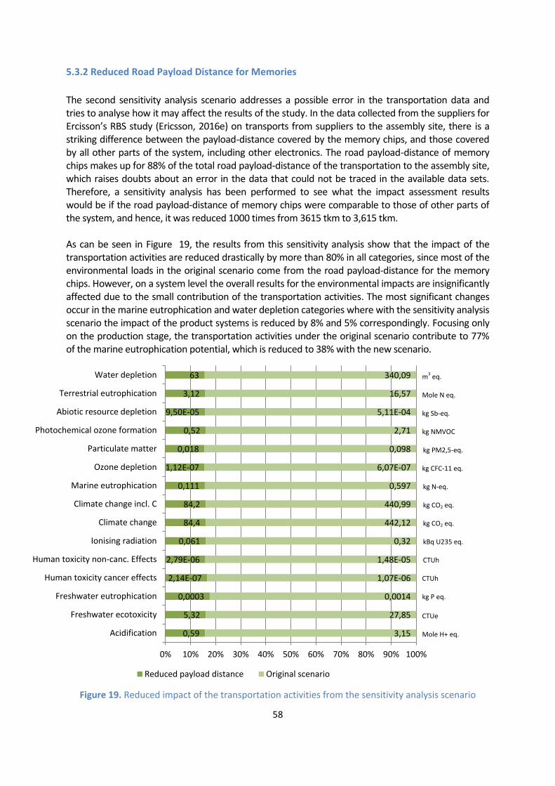
58

5.3.2 Reduced Road Payload Distance for Memories

The second sensitivity analysis scenario addresses a possible error in the transportation data and tries to analyse how it may affect the results of the study. In the data collected from the suppliers for Ercisson’s RBS study (Ericsson, 2016e) on transports from suppliers to the assembly site, there is a striking difference between the payload-distance covered by the memory chips, and those covered by all other parts of the system, including other electronics. The road payload-distance of memory chips makes up for 88% of the total road payload-distance of the transportation to the assembly site, which raises doubts about an error in the data that could not be traced in the available data sets. Therefore, a sensitivity analysis has been performed to see what the impact assessment results would be if the road payload-distance of memory chips were comparable to those of other parts of the system, and hence, it was reduced 1000 times from 3615 tkm to 3,615 tkm. As can be seen in Figure 19, the results from this sensitivity analysis show that the impact of the transportation activities are reduced drastically by more than 80% in all categories, since most of the environmental loads in the original scenario come from the road payload-distance for the memory chips. However, on a system level the overall results for the environmental impacts are insignificantly affected due to the small contribution of the transportation activities. The most significant changes occur in the marine eutrophication and water depletion categories where with the sensitivity analysis scenario the impact of the product systems is reduced by 8% and 5% correspondingly. Focusing only on the production stage, the transportation activities under the original scenario contribute to 77% of the marine eutrophication potential, which is reduced to 38% with the new scenario.

Figure 19. Reduced impact of the transportation activities from the sensitivity analysis scenario

0,59

5,32

0,0003

2,14E-07

2,79E-06

0,061

84,4

84,2

0,111

1,12E-07

0,018

0,52

9,50E-05

3,12

63

3,15

27,85

0,0014

1,07E-06

1,48E-05

0,32

442,12

440,99

0,597

6,07E-07

0,098

2,71

5,11E-04

16,57

340,09

0% 10% 20% 30% 40% 50% 60% 70% 80% 90% 100%

Acidification

Freshwater ecotoxicity

Freshwater eutrophication

Human toxicity cancer effects

Human toxicity non-canc. Effects

Ionising radiation

Climate change

Climate change incl. C

Marine eutrophication

Ozone depletion

Particulate matter

Photochemical ozone formation

Abiotic resource depletion

Terrestrial eutrophication

Water depletion

Reduced payload distance Original scenario

kg Sb-eq.

m3 eq.

Mole N eq.

Mole H+ eq.

CTUe

kg P eq.

CTUh

CTUh

kBq U235 eq.

kg CO2 eq.

kg CO2 eq.

kg NMVOC

kg PM2,5-eq.

kg N-eq.

kg CFC-11 eq.

59

5.3.3 Different Electricity Mixes during the Use Stage

The third scenario aims at performing a sensitivity analysis on the data in the use stage. For this purpose, the different electricity mixes have been alternated in the model to see how this affects the environmental performance of the product system during the assumed five years of usage. Figure 20 shows that, for example, the global warming potential during the operation of the product system may change considerably depending on the type of electricity mix used. In comparison to the originally used global mix descried in Section 4.4.4, Chinese electricity increases the potential impact for climate change in the use stage by 65% and would lead to an increase of 60% in the overall cradle-to-grave impact of the product system in this category. The U.S. and Japanese electricity mixes would also lead to a slight to moderate rise of potential CO2 emissions, while the EU-27 mix would cut the potential impact of the system during its life cycle by one-fifth.

Figure 20. Results on the change of the potential impact of 1 kW electricity use in the climate change impact category (incl. biogenic carbon) from the sensitivity analysis

Changes from alternating the electricity mixes differ in the different impact category. Apart from the effect on climate change, the coal-based Chinese electricity mix increases more than twice the acidification, ecotoxicity, terrestrial eutrophication and photochemical ozone formation potential of the use of the product system, and almost eight times its potential impact in terms of particulate matter, while reducing the ionising radiation potential almost 20 times, and eutrophication in aquatic environments. The U.S. electricity mix, which according to GaBi (PE International, 2016) is mostly hard coal, natural gas and nuclear, increases substantially the ecotoxocity potential and the human toxicity potential with cancer effects. The European electricity mix, which according to GaBi (PE International, 2016) is more diversified (apart from nuclear energy, energy from natural gas, lignite, considerably smaller share of hard

0,59

0,97

0,66 0,62

0,46

0

0,2

0,4

0,6

0,8

1

1,2

Global mix China electricity Japan electricity U.S. electricity EU-27 electricity

13% 5%

21%

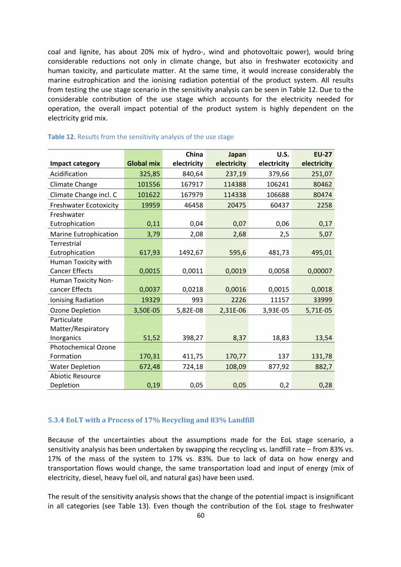
60

coal and lignite, has about 20% mix of hydro-, wind and photovoltaic power), would bring considerable reductions not only in climate change, but also in freshwater ecotoxicity and human toxicity, and particulate matter. At the same time, it would increase considerably the marine eutrophication and the ionising radiation potential of the product system. All results from testing the use stage scenario in the sensitivity analysis can be seen in Table 12. Due to the considerable contribution of the use stage which accounts for the electricity needed for operation, the overall impact potential of the product system is highly dependent on the electricity grid mix. Table 12. Results from the sensitivity analysis of the use stage

Impact category Global mix China

electricity Japan

electricity U.S.

electricity EU-27

electricity

Acidification 325,85 840,64 237,19 379,66 251,07

Climate Change 101556 167917 114388 106241 80462

Climate Change incl. C 101622 167979 114338 106688 80474

Freshwater Ecotoxicity 19959 46458 20475 60437 2258

Freshwater Eutrophication 0,11 0,04 0,07 0,06 0,17

Marine Eutrophication 3,79 2,08 2,68 2,5 5,07

Terrestrial Eutrophication 617,93 1492,67 595,6 481,73 495,01

Human Toxicity with Cancer Effects 0,0015 0,0011 0,0019 0,0058 0,00007

Human Toxicity Non-cancer Effects 0,0037 0,0218 0,0016 0,0015 0,0018

Ionising Radiation 19329 993 2226 11157 33999

Ozone Depletion 3,50E-05 5,82E-08 2,31E-06 3,93E-05 5,71E-05

Particulate Matter/Respiratory Inorganics 51,52 398,27 8,37 18,83 13,54

Photochemical Ozone Formation 170,31 411,75 170,77 137 131,78

Water Depletion 672,48 724,18 108,09 877,92 882,7

Abiotic Resource Depletion 0,19 0,05 0,05 0,2 0,28

5.3.4 EoLT with a Process of 17% Recycling and 83% Landfill

Because of the uncertainties about the assumptions made for the EoL stage scenario, a sensitivity analysis has been undertaken by swapping the recycling vs. landfill rate – from 83% vs. 17% of the mass of the system to 17% vs. 83%. Due to lack of data on how energy and transportation flows would change, the same transportation load and input of energy (mix of electricity, diesel, heavy fuel oil, and natural gas) have been used. The result of the sensitivity analysis shows that the change of the potential impact is insignificant in all categories (see Table 13). Even though the contribution of the EoL stage to freshwater

61

eutrophication increases by 16%, because of the minor impact of this stage it does not affect the overall freshwater eutrophication impact of the product system. At the same time, under ionising radiation, where the assumed EoLT processes affect the environmental performance of the system the most, no change is recorded with the new scenario. The main reason is that, as mentioned earlier, the EoLT model accounts only for the treatment processes and not for the avoided burdens. That is why the potential impact in this life-cycle stage comes mainly from the transportation and the energy sources used in the recycling processes (data on which have been provided from recycling companies for Ercan, et al. (2016)), and landfill has minor contribution. Further discussion on the EoL stage is available in 7.1. Table 13. Results from the sensitivity analysis on the EoL stage

Impact category 83% recycling

vs. 17% landfill 17% recycling

vs. 83% landfill Change of impact in

the EoL stage

Acidification 0,193 0,201 4,15%

Freshwater Ecotoxicity -400 -400 0,00%

Freshwater Eutrophication 0,00657 0,00763 16,13%

Human Toxicity with Cancer Effects 4,97E-07 5,17E-07 4,02%

Human Toxicity Non-cancer Effects -0,000215 -0,000215 0,00%

Ionising Radiation 4,59E+03 4,59E+03 0,00%

Climate Change 66,9 69,1 3,29%

Climate Change incl. C 66,5 68,7 3,31%

Marine Eutrophication 0,0636 0,0638 0,31%

Ozone Depletion 4,25E-07 4,25E-07 0,00%

Particulate Matter/Respiratory Inorganics -0,0132 -0,0128 -3,03%

Photochemical Ozone Formation 0,132 0,137 3,79%

Abiotic Resource Depletion 4,36E-05 4,44E-05 1,77%

Terrestrial Eutrophication 1,02 1,04 1,96%

Water Depletion 106,54 108 1,37%

62

6. Impact on a Network Level The aim of this study is to estimate the potential environmental impacts of the core network, and one of the objectives involved applying the LCA methodology on ICT equipment used for core network functionalities in order to the achieve the above aim. This is based on the principle that ICT networks are systems composed by different types of ICT goods and a network’s aggregated impact equals the sums of the impact from all the ICT goods comprising that network ITU (2014). For the purpose of scaling up the results from the LCA to a network level, data from an internal Ericsson model on dimensioning the mobile network has been used (Singh, 2016). Based on that data, an average scenario for a mobile network of 26 million subscribers is used according to which the core network power consumption is 83 kW. Knowing how much the equipped cabinet under this LCA study consumes, a calculation shows that such a model network needs 21 BSP 8100 from the studied configuration to maintain the core network functionalities. With this data, involving simplifications discussed in Section 7.2, the results from the above LCA study are extrapolated to calculate the potential environmental impacts for the use of the core network by one subscriber per year, as shown in Table 14.

6.1 Impact Assessment Results for the Core Network According to the results, the global warming potential of the whole core network for one year for the coverage of 26 million subscribers is almost 466 kg CO2 eq., while the use of the core network by one subscriber per year accounts for 18 g CO2 eq. For results in other impact categories please refer to Table 14. In comparison, in their recent study Malmodin and Lundén (2016) conclude that the carbon footprint of the mobile network per subscriber is 50 kg CO2 eq. when using a global electricity mix, while Ercan et al. (2016) assess the annual impact of the overall network usage by one subscriber (including mobile and wifi access) to have a global warming potential from 36 to 67 kg CO2 eq. depending on the usage scenario (from low to heavy), again when

using a global electricity mix. As an example of the impact of user equipment, results obtained by Ercan, et al. (2016) show that the GWP of the use of a smartphone with 9.5 cm2 of IC chip area for one year is 19 kg CO2 eq. Table 14. Environmental impacts of the core network

Impact category Units

Total impact of

FU

Core network impact for

5 years

Impact per subscriber for 5 years

Impact per subscriber for 1 year

Normalisation results for the core network impact per

person per year

Acidification Mole of H+ eq. 427,6381 8982,349 0,000345475 6,9095E-05 0,00015%

Climate Change kg CO2 eq. 110868 2328733 0,089566655 0,017913331 n/a

Climate Change incl. C kg CO2 eq. 110542,4 2321894 0,089303615 0,017860723 0,00019%

Freshwater Ecotoxicity CTUe 683098,5 14348182 0,551853169 0,110370634 0,00126%

Freshwater Eutrophication kg P eq. 15,61691 328,0263 1,26164E-05 2,52328E-06 0,00017%

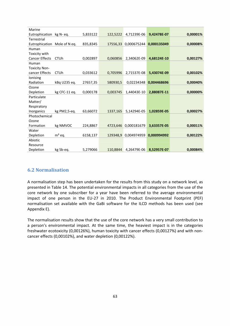
63

Marine Eutrophication kg N- eq. 5,833122 122,5222 4,71239E-06 9,42478E-07 0,00001%

Terrestrial Eutrophication Mole of N eq. 835,8345 17556,33 0,000675244 0,000135049 0,00008%

Human Toxicity with Cancer Effects CTUh 0,002897 0,060856 2,34062E-09 4,68124E-10 0,00127%

Human Toxicity Non-cancer Effects CTUh 0,033612 0,705996 2,71537E-08 5,43074E-09 0,00102%

Ionising Radiation kBq U235 eq. 27657,35 580930,5 0,02234348 0,004468696 0,00040%

Ozone Depletion kg CFC-11 eq. 0,000178 0,003745 1,44043E-10 2,88087E-11 0,00000%

Particulate Matter/ Respiratory Inorganics kg PM2,5-eq. 63,66072 1337,165 5,14294E-05 1,02859E-05 0,00027%

Photochemical Ozone Formation kg NMVOC 224,8867 4723,646 0,000181679 3,63357E-05 0,00011%

Water Depletion m³ eq. 6158,137 129348,9 0,004974959 0,000994992 0,00122%


kg Sb-eq.

5,279066

110,8844

4,26479E-06

8,52957E-07 0,00084%

6.2 Normalisation A normalisation step has been undertaken for the results from this study on a network level, as presented in Table 14. The potential environmental impacts in all categories from the use of the core network by one subscriber for a year have been referred to the average environmental impact of one person in the EU-27 in 2010. The Product Environmental Footprint (PEF) normalisation set available with the GaBi software for the ILCD methods has been used (see Appendix E). The normalisation results show that the use of the core network has a very small contribution to a person’s environmental impact. At the same time, the heaviest impact is in the categories freshwater ecotoxicity (0,00126%), human toxicity with cancer effects (0,00127%) and with non-cancer effects (0,00102%), and water depletion (0,00122%).

64

7. Discussion This section presents further discussion on the study, its limitations and results.

7.1 Discussion on the LCA-based Part of the Study BSP 8100 represents a very complex product system which consists of multiple parts - all of them involving multiple components, with multiple suppliers, in multiple locations all over the globe changing dynamically over time depending on different factors. All these make completing an LCA on such a system a challenging and complex undertaking. Every decision made during the LCA process for every single detail in the modelled scenarios already adds to the relativity of the results, which is especially true for the complex ICT product system as explained by ETSI (2015). In real deployments, configurations depend on the operators’ needs for functionalities covered, equipment capacity, subscriber coverage, population density, etc. Densely populated urban areas allow for optimizing the use of the network equipment, while the least-populated rural regions may require covering vast geographical areas with few network users. In the case of BSP 8100, all these may affect the types and count of processor boards used in a configuration and their corresponding chip area, the number of subracks, the amount of cabling, even the need or not for a cabinet, among others. The choice of suppliers and production sites for all intermediate products of the system defines not only the raw materials acquisition and the transportation models, but also affects the whole production because of local specificities such as energy sources or methods of handling production waste. The choice of deployment sites affects the potential impact of the use stage depending on local electricity mixes (as shown through sensitivity analysis in 5.3) or what the EoLT methods are. As for all ICT LCAs, the limited availability of process-specific data have led the whole cradle-to-grave model to rely to a large extent on generic data available with the databases in GaBi which do not always provide accurate processes. For example, in some cases, location-specific database processes were not available. For instance, a hazardous waste treatment process to use while modelling the production stage was only available for Switzerland, although the process was assumed to take place in Taiwan. This leaves the uncertainty about the treatment method used and how this may affect the results, especially when such a process clearly shows to have major contribution. The raw materials acquisition sub-model is built on overall product system level and not structured per module. This simplified modelling was due to modelling difficulties and puts limitations on the model reusability and prevents detailed break-down of raw materials results on the different modules of the product, such as processor boards, subracks, cables, cabinet, packaging, etc. Modelling based on different product parts of the system would have made it more visible and easily traceable the processes for which modules bring the most potential impact in the raw materials stage which could help identify possible improvements in the products. However, other sources of information, like materials declarations, may resolve this. This simplified structure also limits the reusability of the sub-model for future LCA studies of BSP.

65

For example, even if only small configuration modifications are made, the weight parameters used in the GaBi model may have to be recalculated on a system level for the whole model. Uncertainty of the raw materials acquisition model comes also from the amount of unknown materials and from the unknown extent of recycled materials involved in the secondary data used from the GaBi databases. However, it is known from the GaBi database that modelled systems contains virgin gold and mostly virgin copper, and the results show that their acquisition leads to the heaviest potential impacts during the raw materials stage. Therefore, the input of recycled gold and copper may reduce significantly that impact potential in freshwater ecotoxicity (especially having in mind its larger contribution in the normalized results) and eutrophication, as well as the abiotic resource depletion potential to certain extent. Other uncertainties that should be noted arise from using different databases in GaBi, as shown in Ercan, et al. (2016, p. 129). The authors show how the results for the potential impacts of the product system change when using one or another datasets, in their case Ecoinvent and GaBi which are based on data from different mining models. In this study, both databases were used because of data gaps. Ericsson has a global supply chain with multiple suppliers for the same product. The manufacturing sub-model for this study is based on data for a radio base station (RBS) and uses mostly one supplier for each modelled intermediate product of the system which is another simplification of the real scenario which brings uncertainty. As acknowledged by ETSI (2015) and ITU (2014), the full set of data for all suppliers is beyond reach for ICT product systems. Also, the sales volumes used to allocate the deployment of BSP 8100 with customers and create transportation scenarios per region are based on 3-months data which means they can vary significantly. Another important note to make is that the use stage, which is a major contributor to the potential environmental impacts under a number of impact categories, would give varying results depending on the electricity mix of the deployment location choice. Figure 20 clearly visualizes how for the same amount of electricity used four different electricity mixes (Chinese, Japanese, U.S. and EU-27) have completely different environmental impact potential in all impact categories. Although the current model of the use stage is trying to reflect a certain level of variation to represent a global scenario, it is still simplified. If data from maintenance activities were available and modelled, that would have added to the overall impact of the use stage. The operator activities were left out of the study. A major simplification is applied for the EoL stage, as well. Using a flat rate for the recycling of materials independent on their types is not a realistic scenario in terms of finding out the avoided burdens in the system due to recovery and recycling in this stage. However, as the EoLT scenarios modelled in this study looks at recycling only as a process of EoLT without accounting for the positive effect coming from avoided burden, this simplification does not a major impact on the results. In any case, if data on the recycling rate of different materials were available, a better scenario could have been used. In general, the objective of identifying hotspots of potential environmental impacts caused throughout the life cycle of the studied product system has been only partially achieved. The main reason is the use of secondary data and filling data gaps from databases available with the modelling software. Then, even if processes and flows are identified in the built model as having

66

major impact potential, they usually cannot be related to the actual processes and flows taking place in reality from the cradle to the grave of the assessed product system. The sensitivity analysis performed shows clearly that electronics expressed by the chip area of the integrated circuits contribute significantly to the potential environmental impacts, and in this scenario possible omission of electronic components may have reduced the results. Due to the general trend in electronics of reducing the chip area, this also implies that in the future there are possibilities for decreased impact which are worth to be studied, especially due to their contribution in small user equipment such as the smartphone, as shown in Ercan, et al. (2016). Another important aspect for future studies on the potential environmental impacts of the core network, as well as of the mobile network as a whole, will be shifting the focus from climate change to other impact categories. Deepening the analysis on the implications of these impacts in the context of the areas of protection such as human health, the natural environment and natural resources would highlight better which are the hotspots in the life cycle which need to be addressed with priority.

7.2 Discussion on the Representativeness of the Product System The calculations that allow scaling up the results from this LCA-based study and estimating the potential environmental impacts for the whole core network present a very simplified average model of the network. As mentioned above, the deployment of core network equipment and its coverage depends on multiple factors. For example, a BSP 8100 configuration can serve more subscribers if it is to cover a densely populated urban area, whereas it may not suffice to provide core network support for much fewer subscribers spread out in a rural area. Therefore, the potential impacts of the core network could be both larger or smaller in different cases. What is more, it is important to point out that BSP 8100 is the dominating but not the only Ericsson server platform equipment covering core network functionalities. Also, while the studied product system contains processor blades from one generation (the most widely used at the moment), actual network equipment combines different technologies and also usually uses processor boards from different generations which changes both their power consumption and capacity, and hence, would affect the LCA results. Rapid technology development and the time-consuming data collection phase in LCA make it difficult to keep such studies completely up to date with current technologies. While performing the current study, virtualization on multiple core network applications running on BSP 8100 have been launched (Ericsson, 2016d; Blomqvist, 2015) which reduces the need for dedicated hardware, but also reduces the capacity of the applications. At the same time, a new generation of processor blades is introduced that consumes more energy, but also has much greater capacity (Wägmark, 2015a; Blomqvist, 2016). These launches and the constantly increasing data traffic per user are setting new trends whose potential environmental impacts should also be assessed and monitored in future research.

67

8. Conclusions This LCA-based study has been carried out with the purpose of assessing the potential environmental impacts of the core network for mobile telecommunications covering a whole set of impact categories, but having a focus on climate change. The core network controls the network features and telecommunication services, handles the management of user location information and the transfer mechanisms, both switching and transmission, for signalling and for user generated information. To achieve the aim of this study, the previous knowledge on the environmental impacts of the core network should be investigated, the hardware equipment covering core network functionalities should be identified and the product system for assessment should be selected. Carrying out an LCA study of the selected product system would allow for identifying the hotspots of potential environmental impacts caused throughout the life cycle of that system. These results can be used to estimate the environmental impacts of the whole core network and of its usage by one mobile subscriber per year. In view of the above aim and objectives, the main conclusions from this study are:

An investigation of earlier scientific works on the environmental impact of the mobile network shows that there is a knowledge gap about the contribution of the core network.

The Ericsson BSP (Blade Server Platform) 8100 has been identified as the state-of-the-art equipment that hosts the greatest part of the applications covering core network functionalities, and therefore has been selected for this LCA study. A representative configuration has been used in it.

The LCA study shows that an equipped BSP 8100 cabinet containing the studied configuration releases nearly 111 tonne CO2 eq. during its life cycle, assuming five years of use.

According to the results of this LCA-based study and to an internal Ericsson network dimensioning model, the global warming potential of the whole core network for one year for the coverage of 26 million subscribers is almost 466 tonne CO2 eq.

By using the core network through their mobile device, one subscriber contributes with approximately 18 g CO2 eq. per year. According to other studies, the use of the whole mobile network by a subscriber per year has a carbon footprint of about 50 kg CO2 eq. when using a global electricity mix, while using a smartphone for the same period results in about 20 kg CO2 eq. global warming potential.

The use stage of BSP 8100 dominates in contributing to the potential environmental impacts in nine out of 15 studied impact categories (acidification, climate change with and without biogenic carbon, human toxicity with cancer effects, marine and terrestrial eutrophication, ionising radiation, particulate matter/respiratory inorganics, and photochemical ozone formation).

68

As shown though a sensitivity analysis, due to the considerable contribution of the use stage which accounts for the electricity needed for operation, the overall environmental performance of the product system is highly dependent on the electricity grid mix and therefore, on the deployment location.

The raw materials acquisition stage prevails in contributing to the overall potential impacts of the system in five impact categories (abiotic resource depletion, ozone depletion, human toxicity with non-cancer effects, freshwater eutrophication and freshwater ecotoxicity). In most of these categories, copper and gold cause the biggest impacts.

The production stage contributes mostly to water depletion caused by the applied Chinese electricity grid mix assumed as used by suppliers.

A 30% decrease of the chip area of the integrated circuits in the studied configuration would reduce the potential impacts from the production activities with an average of 11%.

Compared to the above life cycle stages, the EoLT stage, assuming 83% recycling, has minimal environmental impacts potential in most impact categories and most of the impact comes from the transportation and the energy sources used for the recycling processes.

The normalisation results show that the use of the core network has a very small contribution to a person’s environmental impact. At the same time, the heaviest impact is in the categories freshwater ecotoxicity (0,00126%), human toxicity with cancer effects (0,00127%) and with non-cancer effects (0,00102%), and water depletion (0,00122%).

69

References

Public References

3GPP, 2014. 3GPP TS 23.101 V12.0.0. [Online] Available at: <http://www.3gpp.org/ftp/specs/archive/23_series/23.101/23101-c00.zip> [Accessed 3 November 2015].

Arushanyan, Y., Ekener-Petersen, E. and Finnveden, G., 2014. Lessons learned – Review of LCAs for ICT products and services. Computers in Industry, [Online] 65(2), pp. 211-234. Available at: <http://dx.doi.org/10.1016/j.compind.2013.10.003> [Accessed 9 February 2017].

Baumann, H. and Tillman, A., 2014. The Hitch Hiker’s Guide to LCA. Lund: Studentliteratur.

Blomqvist, M., 2015. BSP hardware. [Meetings] (Personal communication, 19 October/10 November, 2015).

C4Media, 2009. The Problem of Power Consumption in Servers. [Online] Available at: <https://www.infoq.com/articles/power-consumption-servers> [Accessed 11 January 2017].Cronebäck, A., 2013. Input interface requirements on board mounted DC/DC converters. [Online] Available at: <http://kth.diva-portal.org/smash/record.jsf?pid=diva2%3A628811&dswid=1591> [Accessed 6 April 2016].

Dahlman, E., Parkvall, S. and Sköld, J., 2014. 4G: LTE/LTE-Advanced for Mobile Broadband. 2nd ed. Oxford: Elsevier.

DistanceFromTo, 2016. Distance Between Cities Places On Map. [Online] Available at: <http://www.distancefromto.net/> [Accessed 13 June 2016].

Donovan, C., 2009. Twenty thousand leagues under the sea: A life cycle assessment of fibre optic submarine cable systems [Online] Available at: <https://www.seed.abe.kth.se/polopoly_fs/1.190775!/Menu/general/column-content/attachment/MScThesDonovan09.pdf> [Accessed 11 January 2016].

EEA, 1997. Life Cycle Assessment (LCA) - A guide to approaches, experiences and information sources. [Online] Available at: <http://www.eea.europa.eu/publications/GH-07-97-595-EN-C/Issue-report-No-6.pdf> [Accessed 24 February 2016].

Ercan, E. M., 2013. Global Warming Potential of a Smartphone: Using Life Cycle Assessment Methodology. [Online] Available through: KTH Library website: <http://kth.diva-portal.org/smash/get/diva2:677729/FULLTEXT01.pdf> [Accessed 25 September 2015].

Ercan, et al., 2016. Life Cycle Assessment of a Smartphone. [Online] Atlantis Press. Available at: <http://www.atlantis-press.com/php/download_paper.php?id=25860375> {Accessed 5 November 2016].

Ericsson, 2016a. Ericsson Mobility Report. [Online] Available at: <https://www.ericsson.com/assets/local/mobility-report/documents/2016/ericsson-mobility-report-november-2016.pdf > [Accessed 2 November 2016].

ETSI, 2014. Network Functions Virtualisation (NFV); Terminology for Main Concepts in NFV. [Online] Available at: <http://www.etsi.org/deliver/etsi_gs/NFV/001_099/003/01.02.01_60/gs_NFV003v010201p.pdf> [19 December 2016].

70

ETSI, 2015. Environmental Engineering (EE); Methodology for environmental Life Cycle Assessment (LCA) of Information and Communication Technology (ICT) goods, networks and services. [Online] Available at: <http://www.etsi.org/deliver/etsi_es/203100_203199/203199/01.03.01_60/es_203199v010301p.pdf > [Accessed 3 November 2016].

ETSI, n.d. Network Functions Virtualization. [Online] Available at: <http://www.etsi.org/technologies-clusters/technologies/nfv> [19 December 2016].

European Union, 2010a. ILCD Handbook - General guide for Life Cycle Assessment – Detailed guidance. [Online] Available at: <http://publications.jrc.ec.europa.eu/repository/bitstream/JRC48157/ilcd_handbook-general_guide_for_lca-detailed_guidance_12march2010_isbn_fin.pdf> [Accessed 16 December 2016].

European Union, 2010b. ILCD Handbook - Framework and Requirements for Life Cycle Impact Assessment Models and Indicators. [Online] Available at: <http://eplca.jrc.ec.europa.eu/uploads/ILCD-Handbook-LCIA-Framework-Requirements-ONLINE-March-2010-ISBN-fin-v1.0-EN.pdf> [Accessed 16 December 2016].

European Union, 2011. ILCD Handbook: Recommendations for Life Cycle Impact Assessment in the European context. [Online] Available at: <http://eplca.jrc.ec.europa.eu/uploads/ILCD-Recommendation-of-methods-for-LCIA-def.pdf > [Accessed 18 June 2016].

European Union, 2012. Characterisation factors of the ILCD Recommended Life Cycle Impact Assessment methods. [Online] Available at: <http://eplca.jrc.ec.europa.eu/uploads/LCIA-characterisation-factors-of-the-ILCD.pdf > [Accessed 16 December 2016].

GlobeFeed.com, 2015. Distance Calculator and Driving Directions South Korea. [Online] Available at: <http://distancecalculator.globefeed.com/South_Korea_Distance_Calculator.asp> [Accessed 13 June 2016].

Google, 2016. Google Maps. [Online] Available at: <https://www.google.com/maps> [Accessed 13 June 2016].

Guinée, J., et al. eds., 2004. Handbook on Life Cycle Assessment. Operational Guide to the ISO Standards. [E-book] Dordrecht: Kluwer Academic Publishers. Available through: KTH Library website <https://www.kth.se/en/kthb> [Accessed 20 October 2015].

Haleplidis, E., et al. eds, 2015. Software-Defined Networking (SDN): Layers and Architecture Terminology. [Online] Available at: <https://www.rfc-editor.org/rfc/pdfrfc/rfc7426.txt.pdf> [Accessed 19 December 2016].

Hellweg, S. and Milà i Canals, L., 2014. Emerging approaches, challenges and opportunities in life cycle assessment. Science, [Online] 6 June, 344(6188), pp. 1109-1113. Available through: KTH Library website <https://www.kth.se/en/kthb> [Accessed 13 January 2016].

ISO, 2006a. ISO 14040 Environmental management -- Life Cycle Assessment – Principles and framework. [Online] Geneva: International Organization for Standardization. Available at: <http://www.iso.org/iso/catalogue_detail?csnumber=37456> [Accessed 1 October 2015].

ISO, 2006b. ISO 14044 Environmental management -- Life Cycle Assessment -- Requirements and Guidelines. [Online] Geneva: International Organization for Standardization. Available at: <http://www.iso.org/iso/catalogue_detail?csnumber=38498> [Accessed 1 October 2015].

71

Itten, R., Frischknecht, R., and Stucki, M., 2012. Life Cycle Inventories of Electricity Mixes and Grid. [Online] Uster: ESU-services Ltd.. Available at: <http://esu-services.ch/fileadmin/download/publicLCI/itten-2012-electricity-mix.pdf> [Accessed 12 January 2017].

ITU, 2014. Recommendation L.1410 (12/14): Methodology for environmental life cycle assessments of information and communication technology goods, networks and services. [Online] Available at:< http://www.itu.int/rec/T-REC-L.1410-201412-I >[Accessed 24 September 2015].

Liebmann, A., 2015. ICT Waste Handling: Regional and Global End-of-Life Treatment Scenarios for ICT Equipment. [Online] Available through: KTH Library website: <http://kth.diva-portal.org/smash/record.jsf?pid=diva2%3A839633&dswid=-3120> [Accessed 11 December 2015].

Malmodin, J., Bergmark, P. and Lundén, D., 2013. The future carbon footprint of the ICT and E&M sectors. [Online] ICT4S. Available at: <http://2013.ict4s.org/wp-content/uploads/paper/Malmodin_et_al_Future_Carbon_Footprint_of_ICT_and_E&M_Sectors.pdf> [Accessed 11 January 2016].

Malmodin, J., et al., 2012. LCA of data transmission and IP core networks, 2012 Electronics Goes Green 2012+. [Online] Berlin, pp. 1-6. Available at: IEEE Xplore Digital Library <http://ieeexplore.ieee.org.focus.lib.kth.se/stamp/stamp.jsp?arnumber=6360437> [Accessed 12 January 2017].

Malmodin, J., et al., 2014. Life Cycle Assessment of ICT. Journal of Industrial Ecology. [Online] 18(6), pp. 829-845. Available at: <http://onlinelibrary.wiley.com.focus.lib.kth.se/doi/10.1111/jiec.12145/epdf> [Accessed 24 September 2015].

Malmodin, J., and Lundén, D., 2016, The energy and carbon footprint of the ICT and E&M sector in Sweden 1990-2015 and beyond. ICT4S-16. [Online] Atlantis Press. Available at: <http://www.atlantis-press.com/php/paper-details.php?id=25860385 > [Accessed 5 November 2016].

Nuss, P., and Eckelman, M., 2014. Life Cycle Assessment of Metals: A Scientific Synthesis. PLoS One. [Online] 9(7), July 7. Available at: <http://dx.doi.org/10.1371/journal.pone.0101298> [Accessed 12 October 2016].

O’Leary, Z., 2014. Doing Your Research Project. 2nd ed. London: SAGE Publications.

Olsson, M., Sultana, S., Rommer, S., Frid, L. and Mulligan, C., 2009. SAE and the Evolved Packet Core – Driving the Mobile Broadband Revolution. 1st ed. Academic Press.

Olsson, M., Sultana, S., Rommer, S., Frid, L. and Mulligan, C., 2013. EPC and 4G Packet Networks – Driving the Mobile Broadband Revolution. 2nd ed. [e-book] Oxford: Elsevier. Available through: KTH Library website < https://www.kth.se/en/kthb> [Accessed 13 January 2016].

PE International, 2012. GaBi 6.0 Manual. Available at: http://www.gabi-software.com/fileadmin/GaBi_Manual/GaBi_6_manual.pdf [Accessed 18 March 2016].

PE International, 2016. GaBi software databases [Accessed 26 July 2016].

Scharnhorst, W., Hilty, L.M, and Jolliet, O., 2006. Life cycle assessment of second generation (2G) and third generation (3G) mobile phone networks. Environment International. [Online] 32(5), pp. 656–675. Available at: ScienceDirect

72

<http://www.sciencedirect.com.focus.lib.kth.se/science/article/pii/S0160412006000328/pdfft?md5=85ef0dd2bace4d0836bb52c6a2e00ad3&pid=1-s2.0-S0160412006000328-main.pdf> [Accessed 12 January 2017].

SDxCentral, n.d.a. Which is Better – SDN of NFV?. [Online] Available at: <https://www.sdxcentral.com/nfv/definitions/which-is-better-sdn-or-nfv/> [19 December 2016].

SDxCentral, n.d.b. Definition of SDN & NFV Network Virtualization. [Online] Available at: <https://www.sdxcentral.com/sdn-nfv-use-cases/virtual-core-and-aggregation/network-virtualization-mobile/> [19 December 2016].

Sea-distances.org, 2016. Sea-distances.org. [Online] Available at: <http://www.sea-distances.org/> [Accessed 13 June 2016].

Shuller, O., 2016. Energy modelling in Gabi 2016 Edition. [Online] Available at: <http://www.gabi-software.com/fileadmin/GaBi_Databases/GaBi_Database_Upgrade_2016_Documents_for_website_upload/Energy_modelling_in_GaBi_2016.pdf> [Accessed 18 December 2016].

Thinkstep, n.d. Description of the ILCD recommendation. [Online] Available at: <http://www.gabi-software.com/support/gabi/gabi-lcia-documentation/ilcd-recommendation/> [Accessed 29 August 2016].

Internal Ericsson References (confidential)

Blomqvist, M., 2016. Consultation on confidentiality of info on BSP for a public report. [Email] (Personal communication, 27 October 2016).

Ericsson, 2010. BYB 501 Cabinet. Available through: Ericsson Product Catalogue <http://prodcat.internal.ericsson.com/> [Accessed 8 June 2016].

Ericsson, 2012a. BYB 501- Modular indoor cabinet. Available through: Ericsson Product Catalogue <http://prodcat.internal.ericsson.com/> [Accessed 8 June 2016].

Ericsson, 2012b. BSP & SPX HW 1.0 Blade Server Platform. Product Package Description. Available through: Ericsson Product Catalogue <http://prodcat.internal.ericsson.com/> [Accessed 9 October 2015].

Ericsson, 2012c. BSP HW 1.0 Hardware Description. Available through: Ericsson Product Catalogue <http://prodcat.internal.ericsson.com/> [Accessed 9 November 2015].

Ericsson, 2015a. EGEM2 Evolved Generic Ericsson Magazine 2: Common Component Information (Internal). Available through: Ericsson Customer Product Information <http://cpistore.internal.ericsson.com/> [Accessed 5 November 2015].

Ericsson, 2015b. BSP Technical Product Description: BSP 8100. Available through: Ericsson Product Catalogue <http://prodcat.internal.ericsson.com/> [Accessed 9 June 2016].

Ericsson, 2015c. GEP5 Generic Ericsson Processor 5. Available through: Ericsson Product Catalogue <http://prodcat.internal.ericsson.com/> [Accessed 5 November 2015].

Ericsson, 2015d. Packing of Unequipped or Equipped Cabinet x/BYB 501 xxx/x. Available through: Available through: GASK <http://gask2web.ericsson.se/> [Accessed 2 February 2016].

73

Ericsson, 2015e. Packaging Instruction. Available through: Available through: GASK <http://gask2web.ericsson.se/> [Accessed 2 February 2016].

Ericsson, 2016b. BSP Hardware Description: BSP 8100. Available through: Ericsson Product Catalogue <http://prodcat.internal.ericsson.com/> [Accessed 13 April 2016].

Ericsson, 2016c. Produced volumes of GEP. Available through: Ericsson Internal Network <http://erilink.ericsson.se/eridoc/erl/objectId/09004cff8748ef1c?docno=1/1485-1/FCP1059152Uen&action=current&format=excel8book> [Accessed 9 June 2016].

Ericsson, 2016d. Ericsson BSP 8000 Roadmap. Available through: Ericsson Product Catalogue <http://prodcat.internal.ericsson.com/> [Accessed 9 June 2016].

Ericsson, 2016e. LCA of a radio base station. Ericsson, unpublished data [Accessed 17 June 2016].

Sandén, B., 2015a. RE: Notes meeting: Details on BSP components for a life cycle assessment 2015-11-11 15:00-16:00. [Email] (Personal communication, 24 November 2015).

Sandén, B., 2015b. RE: Notes meeting: Details on BSP components for a life cycle assessment 2015-11-11 15:00-16:00. [Email] (Personal communication, 1 December 2015).

Sandén, B., 2016. RE: Details on BSP supply chain. [Email] (Personal communication, 7 March 2016).

Singh, A., 2016. Core + RAN Controllers dimensioning. [Email] (Personal communication, 4 April 2016).

Wägmark, A., 2015a. Details on BSP components for a life cycle assessment. [Meeting] (Personal communication, 11 November 2015).

Wägmark, A., 2015b. RE: Notes meeting: Details on BSP components for a life cycle assessment 2015-11-11 15:00-16:00. [Email] (Personal communication, 13 November 2015).

Wägmark, A., 2015c. RE: Can we assist in giving the package area occupied by IC:s on GEP5?. [Email] (Personal communication, 16 and 23 November 2015).

74

Appendices

Appendix A. Hardware Details (Ericsson Internal)

This appendix outlines further hardware details.

(removed for confidentiality)

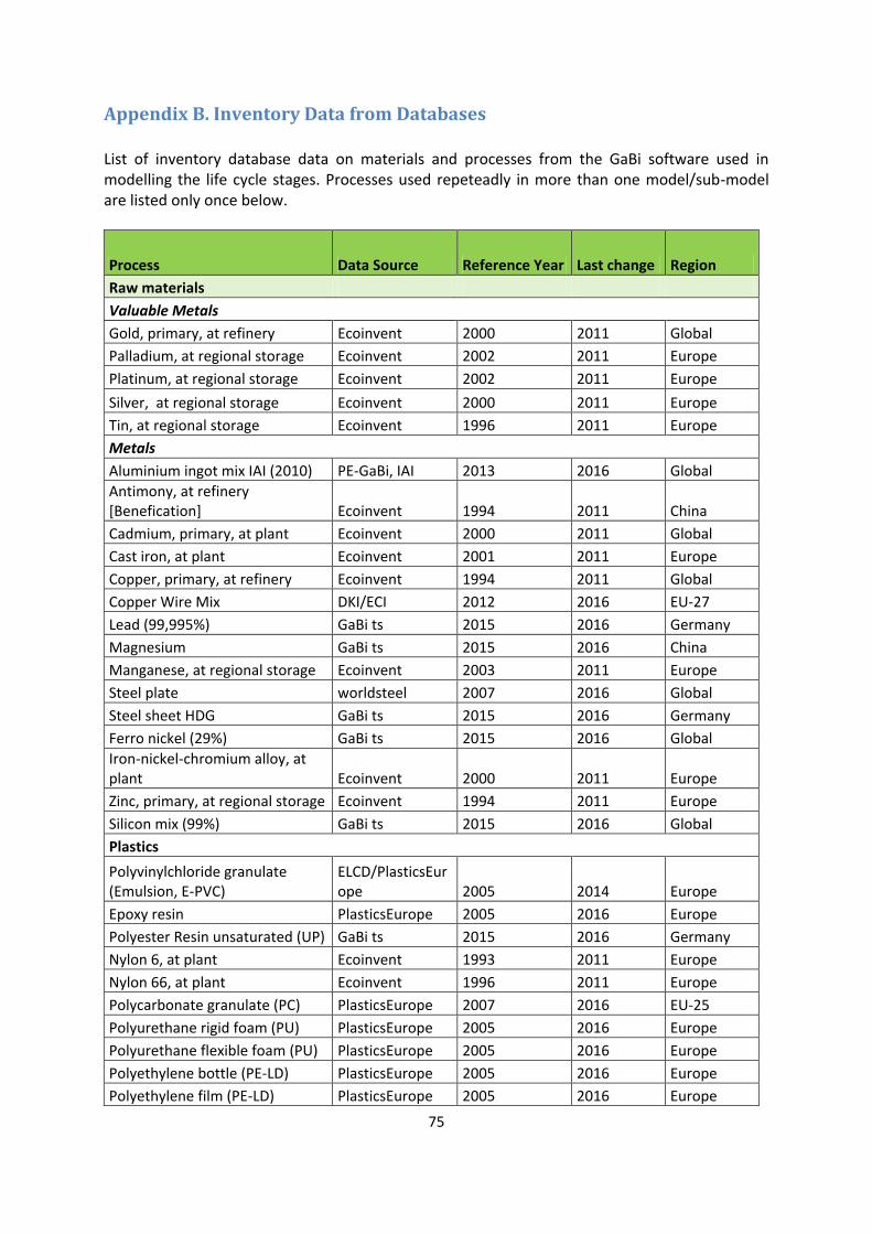
75

Appendix B. Inventory Data from Databases List of inventory database data on materials and processes from the GaBi software used in modelling the life cycle stages. Processes used repeteadly in more than one model/sub-model are listed only once below.

Process Data Source Reference Year Last change Region

Raw materials

Valuable Metals

Gold, primary, at refinery Ecoinvent 2000 2011 Global

Palladium, at regional storage Ecoinvent 2002 2011 Europe

Platinum, at regional storage Ecoinvent 2002 2011 Europe

Silver, at regional storage Ecoinvent 2000 2011 Europe

Tin, at regional storage Ecoinvent 1996 2011 Europe

Metals

Aluminium ingot mix IAI (2010) PE-GaBi, IAI 2013 2016 Global

Antimony, at refinery [Benefication] Ecoinvent 1994 2011 China

Cadmium, primary, at plant Ecoinvent 2000 2011 Global

Cast iron, at plant Ecoinvent 2001 2011 Europe

Copper, primary, at refinery Ecoinvent 1994 2011 Global

Copper Wire Mix DKI/ECI 2012 2016 EU-27

Lead (99,995%) GaBi ts 2015 2016 Germany

Magnesium GaBi ts 2015 2016 China

Manganese, at regional storage Ecoinvent 2003 2011 Europe

Steel plate worldsteel 2007 2016 Global

Steel sheet HDG GaBi ts 2015 2016 Germany

Ferro nickel (29%) GaBi ts 2015 2016 Global

Iron-nickel-chromium alloy, at plant Ecoinvent 2000 2011 Europe

Zinc, primary, at regional storage Ecoinvent 1994 2011 Europe

Silicon mix (99%) GaBi ts 2015 2016 Global

Plastics

Polyvinylchloride granulate (Emulsion, E-PVC)

ELCD/PlasticsEurope 2005 2014 Europe

Epoxy resin PlasticsEurope 2005 2016 Europe

Polyester Resin unsaturated (UP) GaBi ts 2015 2016 Germany

Nylon 6, at plant Ecoinvent 1993 2011 Europe

Nylon 66, at plant Ecoinvent 1996 2011 Europe

Polycarbonate granulate (PC) PlasticsEurope 2007 2016 EU-25

Polyurethane rigid foam (PU) PlasticsEurope 2005 2016 Europe

Polyurethane flexible foam (PU) PlasticsEurope 2005 2016 Europe

Polyethylene bottle (PE-LD) PlasticsEurope 2005 2016 Europe

Polyethylene film (PE-LD) PlasticsEurope 2005 2016 Europe

76

Other materials

Paper, wood-containing, LWC, at regional storage Ecoinvent 2000 2011 Europe

Corrugated board boxes ELCD/FEFCO 2002 2014 EU-25

EUR-flat pallet Ecoinvent 2000 2011 Europe

Plywood, outdoor use, at plant Ecoinvent 1996 2011 Europe

Glass fibres GaBi ts 2015 2016 Germany

Butylene at refinery GaBi ts 2012 2016 GB

Acetic acid from methanol (low pressure carbonylation) GaBi ts 2015 2016 Germany

Alkylbenzene, linear, at plant Ecoinvent 1995 2011 Europe

Methyl-3-methoxypropionate, at plant Ecoinvent 2000 2011 Global

Ethene (ethylene) GaBi ts 2015 2016 Germany

Propene (propylene) GaBi ts 2015 2016 EU-27

Carbon black, at plant Ecoinvent 2000 2011 Global

Ammonia mix (NH3) GaBi ts 2015 2016 EU-27

Benzene mix GaBi ts 2015 2016 EU-27

Liquefied Petroleum Gas (LPG) (70% propane, 30% butane) GaBi ts 2012 2016 EU-27

Production

MANUFACTURING

Energy and Fuels

Electricity grid mix PE-GaBi 2011 2014 China

Thermal energy from natural gas PE-GaBi 2011 2014 EU-27

Steam conversion (mp) PE-GaBi 2011 2014 Global

Natural gas mix PE-GaBi 2011 2014 EU-27

Electricity grid mix PE-GaBi 2011 2014 China

Petrol coke at refinery PE-GaBi 2011 2014 EU-27

Diesel mix at refinery PE-GaBi 2011 2014 EU-27

Electricity grid mix PE-GaBi 2011 2014 Germany

District heating 120-400 kW (Use) PE-GaBi 2013 2014 China

Disposal

Disposal, plastic, consumer electronics, 15.3% water, to municipal incineration Ecoinvent 1994 2011 Switzerland

Disposal, hazardous waste, 25% water, to hazardous waste incineration Ecoinvent 1997 2011 Switzerland

Disposal, industrial devices, to WEEE treatment Ecoinvent 2005 2011 Switzerland

Disposal, paint remains, 0% water, to hazardous waste incineration Ecoinvent 1997 2011 Switzerland

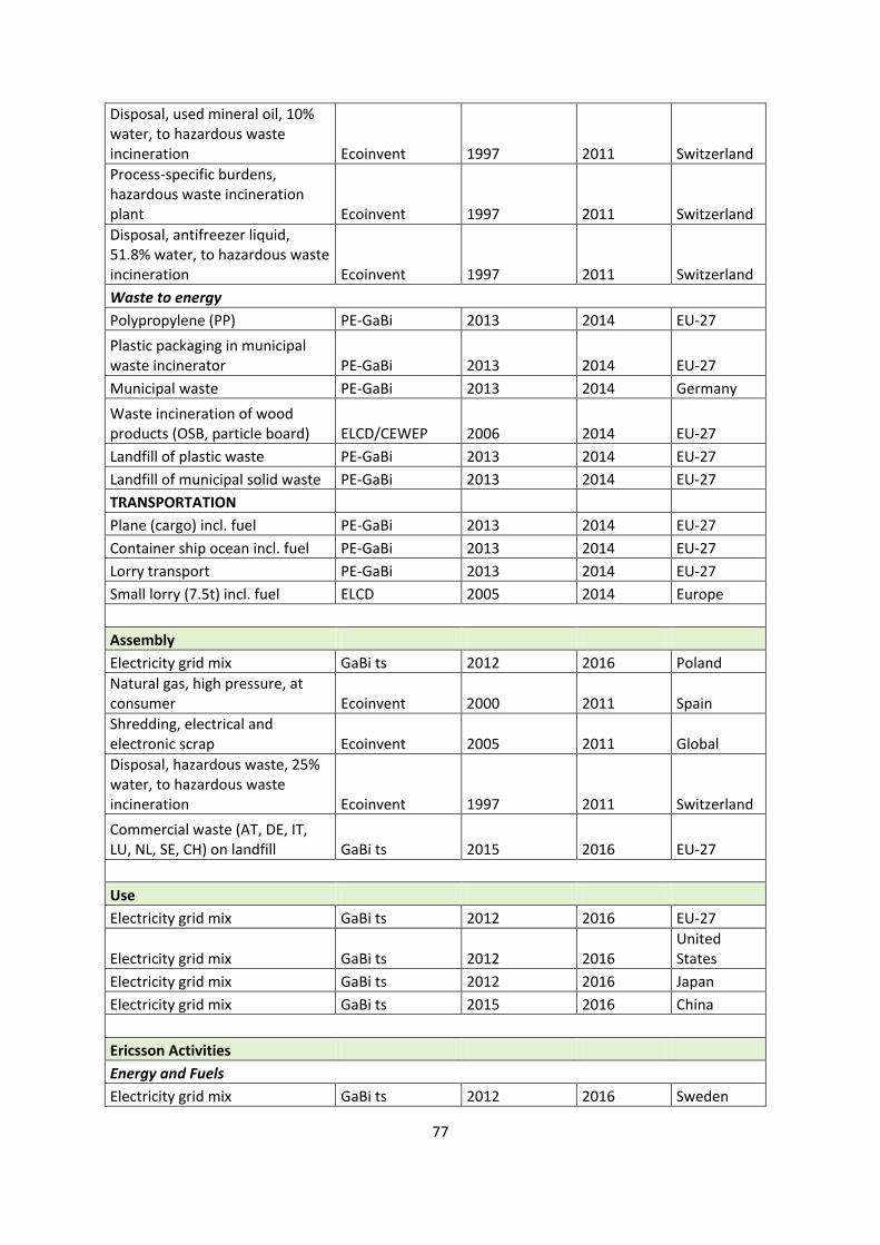
77

Disposal, used mineral oil, 10% water, to hazardous waste incineration Ecoinvent 1997 2011 Switzerland

Process-specific burdens, hazardous waste incineration plant Ecoinvent 1997 2011 Switzerland

Disposal, antifreezer liquid, 51.8% water, to hazardous waste incineration Ecoinvent 1997 2011 Switzerland

Waste to energy

Polypropylene (PP) PE-GaBi 2013 2014 EU-27

Plastic packaging in municipal waste incinerator PE-GaBi 2013 2014 EU-27

Municipal waste PE-GaBi 2013 2014 Germany

Waste incineration of wood products (OSB, particle board) ELCD/CEWEP 2006 2014 EU-27

Landfill of plastic waste PE-GaBi 2013 2014 EU-27

Landfill of municipal solid waste PE-GaBi 2013 2014 EU-27

TRANSPORTATION

Plane (cargo) incl. fuel PE-GaBi 2013 2014 EU-27

Container ship ocean incl. fuel PE-GaBi 2013 2014 EU-27

Lorry transport PE-GaBi 2013 2014 EU-27

Small lorry (7.5t) incl. fuel ELCD 2005 2014 Europe

Assembly

Electricity grid mix GaBi ts 2012 2016 Poland

Natural gas, high pressure, at consumer Ecoinvent 2000 2011 Spain

Shredding, electrical and electronic scrap Ecoinvent 2005 2011 Global

Disposal, hazardous waste, 25% water, to hazardous waste incineration Ecoinvent 1997 2011 Switzerland

Commercial waste (AT, DE, IT, LU, NL, SE, CH) on landfill GaBi ts 2015 2016 EU-27

Use

Electricity grid mix GaBi ts 2012 2016 EU-27

Electricity grid mix GaBi ts 2012 2016 United States

Electricity grid mix GaBi ts 2012 2016 Japan

Electricity grid mix GaBi ts 2015 2016 China

Ericsson Activities

Energy and Fuels

Electricity grid mix GaBi ts 2012 2016 Sweden

78

Electricity grid mix GaBi ts 2012 2016 EU-27

Electricity grid mix GaBi ts 2012 2016 United States

Electricity grid mix GaBi ts 2012 2016 Japan

Electricity grid mix GaBi ts 2015 2016 China

Thermal energy from wood BUWAL 1996 2006 N/A

Thermal energy from natural gas GaBi ts 2012 2016 EU-27

Heavy fuel oil at refinery (1.0wt.% S) GaBi ts 2012 2016 EU-27

Hard coal mix GaBi ts 2012 2016 EU-27

Transportation

Transport, aircraft, passenger, intercontinental Ecoinvent 2000 2011 Europe

Transport, passenger car Ecoinvent 2005 2011 Europe

Office supplies

Laptop computer, at plant Ecoinvent 2001 2011 Global

Paper, wood-containing, LWC, at regional storage Ecoinvent 2000 2011 Europe

End-of-life Treatment

Landfill of ferro metals PE-GaBi 2013 2014 EU-27

Landfill of plastic waste PE-GaBi 2013 2014 EU-27

Energy and Fuels

Electricity, medium voltage, at grid Ecoinvent 2005 2011 China

Electricity mix Ecoinvent 2004 2011 Japan

Electricity mix Ecoinvent 2004 2011 United States

Electricity grid mix PE-GaBi 2011 2014 EU-27

Natural gas mix PE-GaBi 2011 2014 EU-27

Diesel mix at refinery PE-GaBi 2011 2014 EU-27

Heavy fuel oil at refinery (1.0wt.% S) PE-GaBi 2011 2014 EU-27

Transportation

Lorry transport PE-GaBi 2013 2014 EU-27

79

Appendix C. System Flowchart

80

Appendix D. Inventory Data for Raw Materials Acquisition per Part

(removed for confidentiality)

81

Appendix E. Overall Yearly Impact per Person Used for Normalisation The person equivalent of the Product Environmental Footprint (PEF) normalisation set for the ILCD methods with a reference of the EU-27 in the year 2010 available with the GaBi software (PE International, 2016).

Impact category Person

equivalence Unit Factor

Acidification 47,3 Mole of H+ eq. 0,021141649

Climate change incl. C 9220 kg CO2-Equiv. 0,00010846

Freshwater ecotoxicity 8740 CTUe 0,000114416

Freshwater eutrophication 1,48 kg P eq 0,675675676

Marine eutrophication 16,9 kg N-Equiv. 0,059171598

Terrestrial eutrophication 176 Mole of N eq. 0,005681818

Human toxicity cancer effects 3,69E-05 CTUh 27100,271

Human toxicity non-cancer effects 0,000533 CTUh 1876,172608

Ionizing radiation 1130 kBq U235 eq 0,000884956

Ozone depletion 0,0216 kg CFC-11 eq 46,2962963

Particulate matter/Respiratory inorganics 3,8 kg PM2,5-Equiv. 0,263157895

Photochemical ozone formation 31,7 kg NMVOC 0,031545741

Water depletion 81,4 m³ eq. 0,012285012

Abiotic resource depletion 0,101 kg Sb-Equiv. 9,900990099

TRITA -IM-EX 2017:02

www.kth.se