the evolution of. . . the isoperimetric problem - mathematical

THE EVOLUTION OF. . .Edited by Abe Shenitzer and John Stillwell

The Isoperimetric Problem

Viktor Blasjo

1. ANTIQUITY. To tell the story of the isoperimetric problem one must begin byquoting Virgil:

At last they landed, where from far your eyesMay view the turrets of new Carthage rise;There bought a space of ground, which Byrsa call’d,From the bull’s hide they first inclos’d, and wall’d.

(Aeneid, Dryden’s translation)

This refers to the legend of Dido. Virgil’s version has it that Dido, daughter of the kingof Tyre, fled her home after her brother had killed her husband. Then she ended up onthe north coast of Africa, where she bargained to buy as much land as she could enclosewith an oxhide. So she cut the hide into thin strips, and then she faced, and presumablysolved, the problem of enclosing the largest possible area within a given perimeter—the isoperimetric problem. But earthly factors mar the purity of the problem, for surelythe clever Dido would have chosen an area by the coast so as to exploit the shore aspart of the perimeter. This is essential for the mathematics as well as for the progressof the story. Virgil tells us that Aeneas, on his quest to found Rome, is shipwreckedand blown ashore at Carthage. Dido falls in love with him, but he does not return herlove. He sails away and Dido kills herself. Kline concludes [23, p. 135]:

And so an ungrateful and unreceptive man with a rigid mind caused the loss of a potentialmathematician. This was the first blow to mathematics which the Romans dealt.

As for the mathematics of the isoperimetric problem, the Greeks pretty much solvedit, by their standards, when Zenodorus proved that a circle has greater area than anypolygon with the same perimeter. His work was lost. We know of it mainly throughPappus and Theon of Alexandria. Pappus’s introduction to the subject (in his Collec-tion, Book V) is considered a literary masterpiece. To quote Heath [18, p. 389]:

It is characteristic of the great Greek mathematicians that, whenever they were free from therestraint of the technical language of mathematics, as when for instance they had occasion towrite a preface, they were able to write in language of the highest literary quality, comparablewith that of the philosophers, historians, and poets.

We quote Pappus’s introduction from [40, pp. 588–593]:

Though God has given to men, most excellent Megethion, the best and most perfect under-standing of wisdom and mathematics, He has allotted a partial share to some of the unreason-ing creatures as well. To men, as being endowed with reason, He granted that they should doeverything in the light of reason and demonstration, but to the other unreasoning creatures He

526 c© THE MATHEMATICAL ASSOCIATION OF AMERICA [Monthly 112

gave only this gift, that each of them should, in accordance with a certain natural forethought,obtain so much as is needful for supporting life. This instinct may be observed to exist inmany other species of creatures, but it is specially marked among bees. Their good order andtheir obedience to the queens who rule in their commonwealths are truly admirable, but muchmore admirable still is their emulation, their cleanliness in the gathering of honey, and theforethought and domestic care they give to its protection. Believing themselves, no doubt, tobe entrusted with the task of bringing from the gods to the more cultured part of mankinda share of ambrosia in this form, they do not think it proper to pour it carelessly into earthor wood or any other unseemly and irregular material, but, collecting the fairest parts of thesweetest flowers growing on the earth, from them they prepare for the reception of the honeythe vessels called honeycombs, [with cells] all equal, similar and adjacent, and hexagonal inform.

That they have contrived this in accordance with a certain geometrical forethought we maythus infer. They would necessarily think that the figures must all be adjacent one to another andhave their sides common, in order that nothing else might fall into the interstices and so defiletheir work. Now there are only three rectilineal figures which would satisfy the condition,I mean regular figures which are equilateral and equiangular, inasmuch as irregular figureswould be displeasing to the bees. [Pappus goes on to argue that only triangles, squares orhexagons fit around a point.] . . . the bees in their wisdom chose for their work that which hasthe most angles, perceiving that it would hold more honey than either of the two others.

Bees, then, know just this fact which is useful to them, that the hexagon is greater thanthe square and the triangle and will hold more honey for the same expenditure of material inconstructing each. But we, claiming a greater share in wisdom than the bees, will investigate asomewhat wider problem, namely that, of all equilateral and equiangular plane figures havingan equal perimeter, that which has the greater number of angles is always greater, and thegreatest of them all is the circle having its perimeter equal to them.

Apart from fascination with bees, motivation for the isoperimetric problem camefrom astronomy. Theon’s account of Zenodorus’s proof is found in his commentary onPtolemy’s Almagest. (Incidentally, Arabic work on isoperimetry was also motivatedby an interest in astronomy.) So let us quote Ptolemy (although the point he makes isnot very clear):

The following considerations also lead us to the concept of the sphericity of the heavens.No other hypothesis but this can explain how sundial constructions produce correct results;furthermore, the motion of the heavenly bodies is the most unhampered and free of all motions,and freest motion belongs among plane figures to the circle and among solid shapes to thesphere; similarly, since of different shapes having an equal boundary those with more anglesare greater [in area or volume], the circle is greater than [all other] surfaces, and the spheregreater than [all other] solids; [likewise] the heavens are greater than all other bodies.

(Almagest, Toomer’s translation [41])

We must also mention that, apparently, it was a common belief in ancient times thatthe perimeter of a figure determines its area. Proclus says:

Such a misconception is held by geographers who infer the size of a city from the length ofits walls. And the participants in a division of land have sometimes misled their partners inthe distribution by misusing the longer boundary line; having acquired a lot with a shorterboundary and so, while getting more than their fellow colonists, have gained a reputation forsuperior honesty.

(Commentary on the Elements, Morrow’s translation [29])

Gandz [14, p. 107] speculates that this may already have stimulated Babylonian math-ematicians:

June–July 2005] THE EVOLUTION OF. . . 527

The typical form of all the quadratic equations in Babylonian mathematics was: Given is theperimeter, x + y = a, and the area, xy = b; to find the length, x , and the breadth, y. . . . Thegreat probability is, in the writer’s opinion, that the origin of this archaic type of quadraticequations is to be seen as the effect of the aforementioned schemes of those who tried to cheatthe plain man in the computation of the capacity of the area.

Zenodorus’s polygon proof. We will now see how Zenodorus proved that a circlehas greater area than any polygon with the same perimeter.

Theorem. For regular polygons with the same perimeter, more sides imply greaterarea.

Proof. Consider the apothem, the radius-like perpendicular drawn from the center toa side (see Figure 1).

Figure 1.

Half the product of the apothem by the fixed perimeter yields the area of the polygon:

=

Figure 2.

The apothem is the height of the triangle in Figure 3:

Figure 3.

If we increase the number of sides, the base of the triangle in Figure 3 is shortenedand the angle is decreased. It is clear that its height increases. We would prove this bytrigonometry; Zenodorus had to rely on the usual pretrig bag of tricks. It is routine forus, and it probably was for Zenodorus as well.

We would all be very surprised if this next theorem did not follow from the previousone, but Zenodorus’s proof is so delightful that we include it anyway.

Theorem. A circle has greater area than any regular polygon with the same perimeter.

Proof. Archimedes proved that the cut-and-roll area formula also holds for the circle(Figure 4).

=

Figure 4.


So we must show that the apothem of any regular polygon is shorter than the radiusof the circle with the same perimeter. Rescale the polygon so that it circumscribes thecircle (Figure 5):

Figure 5.

The perimeter is now greater than the perimeter of the circle, and therefore greater thanbefore the scaling. Thus the scaling was a magnification, with the apothem magnifiedto the size of the radius of the circle.

And now comes the key theorem. Following Zenodorus, we tacitly assume thatamong all n-gons with given perimeter there is (at least) one that has greater area thanall the others. We will say more about this later.

Theorem. A regular n-gon has greater area than all other n-gons with the sameperimeter.

Proof. Among isoperimetric triangles with the same base, the isosceles triangle coversthe greatest area,

>

Figure 6.

so the maximal n-gon must be equilateral. Otherwise we could improve on it by mak-ing it equilateral.

Figure 7.

We now know that the maximal n-gon must be equilateral. Suppose that it is notequiangular. Consider two dissimilar triangles like those in Figure 8:

Figure 8.

Now make them similar by redistributing perimeter from the pointy to the blunt angleuntil the two angles are the same, as shown in Figure 9:

Figure 9.


This increases the area. Accordingly, the maximal n-gon must be equiangular: if not,we could improve on it.

For the second part of this argument we need the lemma that, if two isoscelestriangles have different bases but their other sides equal, then their total area is in-creased when they are made similar as described in the proof. Apparently, Zenodorusphrased his lemma more generally by admitting any two dissimilar isosceles triangles(i.e., by not taking advantage of what we showed earlier, namely, that the maximaln-gon is equilateral). This generalization is false.1 We could ignore that mistake—thegeneralization is pointless anyway—but to a mind less influenced by the Euclideantradition the whole scheme for proving equiangularity seems very unnatural.

In view of Zenodorus’s imperfections, the contributions of the Arabs—al-Khazinand others after him—are quite respectable, but we will not discuss them here, sincetheir inventiveness is also constrained by the Euclidean straitjacket. Similar approachesprevailed stubbornly until the eighteenth century (for example, we will see that there isvery little difference between the first two theorems that we stated and the discussionof these very theorems in the work of Galileo [13]).

2. PRELIMINARIES. In this section we take care of a few things that will be com-mon to many subsequent proofs. First, the problem itself:

The Isoperimetric Problem. Among all figures with a given perimeter L, which oneencloses the greatest area A?

Ruining the suspense, we reply:

The Isoperimetric Theorem. The answer is the circle of circumference L.

To the joy of analysts everywhere, we can rephrase this theorem as an inequality:

The Isoperimetric Inequality. L2 − 4π A ≥ 0, with equality only for the circle.

Sometimes we will find it natural to deal instead with the dual isoperimetric prob-lem: Among all figures with a given area A, determine the one that has the shortestperimeter. This is clearly equivalent to the isoperimetric problem, and the bridge be-tween them is scaling. For suppose the circle solves only the dual problem. That wouldmean that there is some figure with the same perimeter as the circle but with greaterarea. Rescale this figure so that it has the same area as the circle. But the rescaled figurehas a shorter perimeter, a contradiction. Also, obviously, the isoperimetric inequalitydoes not discriminate between the original problem and its dual.

1To maximize the area of two isosceles triangles on given bases, we should not aim to make the anglesequal but to achieve the following relation between the base angles α, β and the bases a, b:

sin α : sin β = a : b.

This is shown geometrically by Steiner [38], who says it had already been shown by Lhuilier [27] using dif-ferential calculus. A counterexample to Zenodorus’s lemma might then look something like Figure 10:

Figure 10.


Here is a lemma that will save us a lot of fuss:

The convexity lemma. A solution to the isoperimetric problem must be convex.

Proof. Suppose it is not. Then taking the convex hull—that is, snapping a rubberband around it and taking that as the new figure—increases the area and decreasesthe perimeter.

Some of our analytic approaches will use the area formula

A(D) = 1

2

∫∂ D

x dy − y dx =∫

∂ Dx dy =

∫∂ D

−y dx .

Being geometers at heart, we refuse to think of this as a corollary to Green’s theorem.Instead, we derive it from its discrete analogue (which will also come in handy). Webegin with triangles.

= −

= − 1

2

(+ +

)

= − 1

2

(−

)

= 1

2

(−

)That is, the area of a triangle T , say in the first quadrant, with vertices (for simplic-

ity) (0, 0), (x1, y1), and (x2, y2) labelled counterclockwise, is given by

A(T ) = x1 y2 − y1x2

2.

In general, this is the signed area, as we see by labelling the vertices clockwise instead.For the area of an n-gon P with its vertices (0, 0), (x1, y1), (x2, y2), . . . , (xn, yn) la-belled counterclockwise we obtain, by subdividing P into coherently oriented trianglesand summing their signed areas,

A(P) = 1

2

n−1∑k=1

xk yk+1 − yk xk+1.

Here is how the signed area takes care of a pathological case:

− + =

Taking the limit in the formula for A(P), we get the area for any figure D with suitablysmooth boundary ∂ D:

A(D) = 1

2

∫∂ D

x(y + dy) − y(x + dx) = 1

2

∫∂ D

x dy − y dx .


3. STEINER. We come now to the hero of our story—Jakob Steiner. From the timeof Descartes, it had been an explicit aim to reduce the solving of geometrical problemsto algebraic calculation, so that the method of solution would be mechanical and gen-eral. This scheme was of course enormously successful, and the mathematics it led tois truly a powerful weapon, even in the hands of simpletons. But fiddling with formulashas romanticizing consequences, so we should expect there to have been nineteenth-century mathematicians who put up a fight for geometry. There were, and Steiner wasone of them. Needless to say, the battle was lost.

The undertone of rebellion is present in the biographical note on Steiner byGeiser [15]:

Unfortunately, the academic history writing also has its Achilles heel, it’s not for nothing thatit is called “Eloges” in France. The cool, distinguished tone requires restraint in all doubtfulpoints and contradictions that cannot be worked around are put in the most refined wording,like the laughter of von Munchhausen in Immermann’s novel, who, as we all know, eventuallylaughed in such a refined manner that no one could notice it anymore. In this way, thesespeeches of praise bring to mind modern holy pictures, where the most splendid aniline colorsare used to augment picturesque drapery with magenta and azure; that the long blonde curlsthen appear in a most ornate arrangement need not be said.

Not all heads are suitable as models for such paintings—where, for instance, would onefind the comb to shape Jakob Steiner’s wild hair into academic fashion?

Steiner gave five proofs of the isoperimetric theorem. Lovely as they are, he leftone point open to attack: all proofs assume the existence of a solution (his strategy isalways to take a figure that is not a circle and show that its area can be improved). Thisdid not go unpunished. The analyst vultures can smell an existence assumption frommiles away. To this day, many authors, revealing their sympathies, are eager to pointout that existence is nontrivial. Perron [30] at least jokes about it:

Theorem. Among all curves of a givenlength, the circle encloses the greatestarea.

Theorem. Among all positive integers,the integer 1 is the largest.

Proof. For any curve that is not a circle,there is a method (given by Steiner) bywhich one finds a curve that enclosesgreater area. Therefore the circle has thegreatest area.

Proof. For any integer that is not 1, thereis a method (to take the square) by whichone finds a larger positive integer. There-fore 1 is the largest integer.

After having gone to a lot of trouble to rigorize Steiner’s first proof with the help ofsome ugly calculations, Blaschke [1, p. 32] asks himself what Steiner, “who was not afriend of excessive politeness,” would say about this. At best, says Blaschke, he wouldhave quoted Faust:

For thus your mind is trained and braced,In Spanish boots it will be laced,That on the road of thought maybeIt henceforth creep more thoughtfully,. . . . . . . . . . . . . . . . . . . . . . . . . . . . . .Who would study and describe the living, startsBy driving the spirit out of the parts:In the palm of his hand he holds all the sections,Lacks nothing, except the spirit’s connections.

(Goethe’s Faust, Kaufmann’s translation)


We could also suggest our old friend Dido’s last words from the Purcell opera:

Remember me, but ah! forget my fate.

Steiner’s first article on the isoperimetric problem [36] clearly assumes the exis-tence of a solution without any indication that this must be proved. I suppose thatthe criticism followed this publication. The following nonsense passage from his nextarticle [37] should perhaps be seen as a halfhearted attempt to silence the critics.

It is clear that there are, for a given perimeter, infinitely many figures of different form, whichmay also have different areas. Nevertheless, it is clear that the area, though it can be made ar-bitrarily small, cannot be made arbitrarily large, for one can always give a figure, proportionalto the perimeter, that exceeds their area. Such a figure is for example the circle that has itsmidpoint on the perimeter and its radius equal to half the given perimeter. But when, for thesame given perimeter, figures can have different areas, while these cannot be arbitrarily large,there must necessarily be either one figure that has greater area than all others or there mustbe several, differently shaped figures that have this property in common, i.e. that have equalarea among themselves, but greater area than all the others.

That said, we will see that there are good reasons for considering Steiner’s proofs tobe essentially complete after all.

We will discuss Steiner’s five proofs and try to show that they contain essentiallythree distinct ideas. All five proofs are presented in two articles published in 1842 [37],[38]. These articles are French translations. The German originals are published onlyin Steiner’s collected works [39] (edited by Weierstrass, who complains in his prefacethat the French translations are not very good and that they introduce several errorsthat are not in the originals). The proof that is fifth in these articles had already beenpublished in 1838 [36].

Steiner’s four-hinge proofs.

Theorem. Any figure with maximal area must be a circle.

Proof. Take a figure with maximal area. Cut its perimeter in half with a line. This linewill split the area in half as well, because if it did not we could take the half withthe greater area together with its reflection in the line and get a figure with the sameperimeter but greater area (Figure 11).

Figure 11.

Consider one of these halves. Suppose it is not a semicircle. Then there will be somepoint on the boundary where lines drawn from the points on the symmetry line meetat an angle that is not a right angle.

Figure 12.


Think of there being a void inside the triangle and think of the pieces on the sides asglued on. Slide the endpoints along the symmetry line to make the angle a right angle(Figure 13).

Figure 13.

This increases the area, so reflecting this gives a figure with greater area while theperimeter is still the same. That is impossible, so the halves must be semicircles andour figure must have been a circle to begin with.

If we draw the triangles together with their reflections then we get quadrilaterals,and we can then see the four hinges that have given the proof its name (Figure 14).Also, we could use reflection in the midpoint of the symmetry line instead, so that thequadrilateral becomes a parallelogram. Perhaps it is slightly more intuitive to arguethat straightening out the parallelogram increases the area.

Figure 14.

Unlike Steiner, we cannot help being a bit curious as to whether this process con-verges. The answer is that it does, and to the circle, no less. This will be proved later.

The proof also works for showing that an optimal 2n-gon must be regular. Supposeit is not. Then, when we cut the figure in half by drawing the line from vertex 1 tovertex n + 1, some vertex will not be on the semicircle from vertex 1 to vertex n + 1and we can apply Steiner’s method there and get a better, isoperimetric 2n-gon.

We will not discuss the second and third proofs as they are based on essentially thesame idea as the first and are not as beautiful. The second proof, for instance, takesthe detour of showing that if we are given four sticks to make a quadrilateral, then,to maximize the area, we should put the vertices on a circle. Then, sure enough, thetheorem follows, for if there were any four points on the optimal figure that were noton a circle, then we could improve on it (Figure 15).

Figure 15.

Steiner’s mean boundary proof.



Proof. Given two curves, consider the mean curve—the curve that stays halfway be-tween the two curves at all times (Figure 16).

Figure 16.

The length of this curve will be less than the mean length of the two given curves(or equal if the two curves are the same), as we can see by slicing the curves intoinfinitesimals and confirming the claim piecewise (Figure 17).

Figure 17.

Take a figure with maximal area and cut its perimeter in half with a line.

Figure 18.

As before, the line will split the area in half as well, because if it did not we could takethe half with the greater area together with its reflection in the line and get a figurewith the same perimeter but greater area. Suppose the two halves are not reflections ofeach other. Then reflect them to the same side and draw the mean curve (Figure 19).

Figure 19.

This mean curve is shorter. But it encloses the same area, for it contains all the areathat the two curves have in common and then half the additional area of the first curveand half the additional area of the second. However, these additional areas are just aslarge, ensuring that the mean curve actually encloses as much area as the the othercurves.

So when we cut the perimeter of a maximal figure in half, the halves cannot bedifferent in shape: if they were, then we could use this construction to get a figure withthe same area and smaller perimeter. Thus the maximal figure cannot be anything otherthan a circle.


Steiner’s snowball-packing proof. Grab a handful of snow. Put one hand on eitherside and compress the snow. Repeat this from all angles. You end up with a snowball.Why is it a ball? Because packing the given amount of snow tighter and tighter mini-mizes the surface area. We now do the same thing for plane figures, packing their areatighter and tighter, thus minimizing the perimeter.


Proof. We begin with a convex figure and wish to modify it so that it becomes sym-metric in a line. To do this, we think of the figure as consisting of vertical slices, andthen we slide each of these slices so that half of each slice lies on either side of theline. If, for now, we consider only polygons, then the process is more down-to-earth,for we can determine the effect by examining what happens to the vertices:

Figure 20.

The area is still the same, but as we see, triangles and trapezoids map to isosceles ones,and these, as we know, cover area more efficiently.

Figure 21.

For polygons then, the perimeter has decreased unless all triangles and trapezoidsare already isosceles, which occurs when the original figure is symmetric in the line(up to a translation). Applying this to infinitesimals, we are persuaded that the sameis true for any convex figure. Thus a solution must be symmetric in every direction,for otherwise we could improve on it. We feel that such a figure must be a circle. Wecan see this a bit more rigorously as follows. Take such a figure. It will be unaffected(up to translation) if we make it symmetric in the x-axis and then in the y-axis. Butnow it must be symmetric in every line through the origin. Surely it must be a circle.Pedantically, consider a point inside the figure and reflect it in all lines through theorigin to show that all other points at the same distance from the origin must also beinside the figure.

For the question of convergence, and for the mathematical modelling of snowball-packing, it is interesting to start with an arbitrary figure and see if repeated symmetriza-tions make it into a circle (Figure 22).


Figure 22.

Quite obviously, this process does in fact converge to a circle, and Steiner pretty muchsays so, even though convergence is not in his vocabulary. This is the most tellingpassage [36, p. 285]:

[T]he difference between the smallest and the largest diameter decreases, for by the process,when the new axis is chosen (as long as it is not parallel to the prior ones), the largest diameterwill be made smaller and the smallest will be made larger, as is easy to see. By appropriatechoices of the new axes, the diameters can be brought closer to equality faster.

It is also implicit in what follows that Steiner considers it obvious that such clev-erly chosen symmetrizations will always give improvements that are substantial, inthe sense that the process will not halt prematurely before it reaches the circle. ThusSteiner knew—though he could perhaps have argued more convincingly, were he notsuch a principled anti-analyst—that we can begin with any figure, make it better andbetter and, in the limit, end up with a circle. This, of course, would prove the isoperi-metric theorem without any assumption of existence.

4. THE CALCULUS OF VARIATIONS. The solution of the isoperimetric problemby means of the calculus of variations was the first proof unhampered by Euclideansterility, and we will try to present it as such, following Euler’s account from 1744 [11].This stands in contrast to the modern theory of the calculus of variations, which haslong been saturated with rigor and analytic trickery.

The question of the existence of a solution also belongs here. Weierstrass provedexistence in his lectures on the calculus of variations in 1879, and with that the firstrigorous solution of the isoperimetric problem was completed. Weierstrass never pub-lished these results. We must rely on the volume on the calculus of variations in hiscollected works [42], which is reconstructed from lecture notes of his students.

This is what Weierstrass has to say about Steiner’s proofs [42, pp. 259–260]:

A detailed discussion of this [the isoperimetric] problem is desirable, since Steiner was ofthe opinion that the methods of the calculus of variations were not sufficient to give a com-plete proof. [Weierstrass notes what Steiner has proved.] But the calculus of variations is in aposition to prove all this, as we will show later; furthermore it can show what Steiner couldnot—that such a maximum really exists. In many cases this can be proved by geometric meansas well, but when, for example, asked for the curve that for a given perimeter encloses thegreatest area (with no further conditions), Steiner draws a line that cuts the perimeter in halfand shows by symmetrizing the figure around this line that a curve of greater area is createdif this line is not a symmetry axis; now it is clear that only for the circle do such lines havesuch properties, but this does not prove that there is an actual maximum, and not just an upperbound.


Theory. Here is the basic idea. Take a curve and wiggle it a little bit, while keeping itsperimeter fixed. If the curve is the one with maximal area then we are at an optimum, soan infinitesimal wiggle will cause zero change in the area. In order to find the optimalfigure, therefore, we calculate the change in area caused by an infinitesimal wiggle andset this equal to zero. This leads to a differential equation that must be satisfied by anoptimal figure, and indeed that is satisfied only by circles.

Forget about isoperimetry for a while and consider the simpler problem of findinga function y(t) that extremizes an integral that depends on it, say∫

F(y, y, t) dt.

(The archetypal example is the brachistochrone problem—the problem of finding thecurve of quickest descent from one point to another—where y(t) is the curve and theintegral is an expression with gravity and stuff in it that says how long it takes for aball to roll down.) Split the t-axis into �t-segments, and let y(t) be linear on these.

Figure 23.

The functions y(t) and y(t) are then determined by the value of y(t) at the breakpoints, call them y1, y2, y3, . . . . Suppose that y(t) is the optimal curve. Grab one ofthese points yk , pull it up and down, and try to feel it click at the optimum. This occurswhen the rate of change in the integral caused by the change in yk is zero (i.e., whenan infinitesimal change in yk results in a zero change in the integral).

Figure 24.

Say we increase yk by dyk . What happens to the integral (which is now really asum)? First, there is the direct change caused by the change in yk , namely,

dyk

(∂ F

∂yk

).

Then there are the changes caused by the changes in the derivatives on the sides of yk ,call them yk and yk+1. When yk changes by dyk , yk changes by dyk/�t , so it causesthe change in the integral

dyk

(1

�t

∂ F

∂ yk

).

Similarly, yk+1 changes by −(dyk/�t) and causes the change

−dyk+1

(1

�t

∂ F

∂ yk+1

).

We infer that the equation for the total change to be zero is

∂ F

∂yk− 1

�t

(∂ F

∂ yk+1− ∂ F

∂ yk

)= 0.


Taking the limit and applying this everywhere (for all t) we get the Euler equation2

∂ F

∂y− d

dt

(∂ F

∂ y

)= 0.

We look for solutions by solving this differential equation.To deal with the isoperimetric problem we need a variation of this idea. We are

looking for the curves t �→ (x(t), y(t)) that maximize the area∫A(x, x, y, y, t) dt = 1

2

∫x y dt − yx dt

while the perimeter ∫L(x, x, y, y, t) dt =

∫ √x2 + y2 dt

is kept fixed. As before, a solution must be such that if we wiggle it infinitesimallywhile keeping the perimeter fixed (that is, the change in the perimeter integral is zero),then because we are at an optimum the change in the area integral is also zero. Wewill consider variations in x(t) and y(t) separately; of course, the two are analogous.Accordingly, we should make an infinitesimal change in y(t) that leaves the perimeterthe same. Our old procedure of changing just one point will not do. Instead, we changetwo points, yk and yk+1 (Figure 25).

Figure 25.

The equation for the change in the perimeter to be zero is then

dyk

(∂L

∂yk− 1

�t

(∂L

∂ yk+1− ∂L

∂ yk

))+ dyk+1

(∂L

∂yk+1− 1

�t

(∂L

∂ yk+2− ∂L

∂ yk+2

))= 0.

At the same time, the change in the area should also be zero

dyk

(∂ A

∂yk− 1

�t

(∂ A

∂ yk+1− ∂ A

∂ yk

))+ dyk+1

(∂ A

∂yk+1− 1

�t

(∂ A

∂ yk+2− ∂ A

∂ yk+2

))= 0.

Let’s write these last equations a bit more compactly as

dyk�Lk + dyk+1�Lk+1 = 0, dyk�Ak + dyk+1�Ak+1 = 0.

These equations capture the essence of a solution, but we will go a bit further, usinga trick to combine them into one simple equation. Suppose that we have a solution.In this case, let λ be the number by which one has to multiply �Lk to get �Ak . Nowsubtract λ times the first equation from the second,

dyk (�Ak − λ�Lk) + dyk+1 (�Ak+1 − λ�Lk+1) = 0.

2Also called the Euler-Lagrange equation. Lagrange [25] in 1762 used a dull analytic approach that becamefashionable with the nineteenth century wave of rigor and has kept its lead over Euler’s approach ever since.


Since the first term is zero, the second term must also be zero. Applying this forall values of k, we see that for a solution we must have �Ai − λ�Li = 0, with thesame λ for all i . Taking the limit, we arrive at the differential equation that describesthe solution:

∂(A − λL)

∂y− d

dt

(∂(A − λL)

∂ y

)= 0.

Similarly, we obtain an equation satisfied by x(t):

∂(A − λL)

∂x− d

dt

(∂(A − λL)

∂ x

)= 0.

But these are the equations we would have arrived at if we were looking for uncon-strained extrema of

∫A − λL . In other words, the problem of extremizing

∫A while

keeping∫

L fixed is the same as that of extremizing∫

A − λL without side conditions,for some λ. This is what is called “Euler’s rule.”

In our investigation of the isoperimetric problem, we could not help solving themore general problem of extremizing pretty much any old integral while another iskept fixed, so perhaps we should forgive the calculus of variations people for callingany such problem an “isoperimetric problem.”

Calculations. We now apply the rules we have found to the isoperimetric problem.


Proof. To maximize the area

1

2

∫x y dt − yx dt

while the perimeter

∫ √x2 + y2 dt

is kept fixed, we should form the function

F = 1

2(x y dt − yx dt) − λ

√x2 + y2

and look for unconstrained extrema of ∫F dt.

We will find the extrema by solving the Euler equations

∂ F

∂x− d

dt

(∂ F

∂ x

)= 0,

∂ F

∂y− d

dt

(∂ F

∂ y

)= 0.


These are

1

2y − d

dt

(−1

2y − λ

x√x2 + y2

)= 0,

−1

2x − d

dt

(1

2x − λ

y√x2 + y2

)= 0.

If t is taken to be an arclength parameter, then these equations simplify to

y + λx = 0, −x + λy = 0,

and their solutions are

x = x0 + λ cost − t0

λ, y = y0 + λ sin

t − t0

λ.

These are plainly parametric equations for a circle.

Following Weierstrass [42, pp. 70–75], we also give a proof along these lines of theisoperimetric theorem for polygons. For this, we need only the discrete versions of theforegoing theory, and then we are supposed to call it not the calculus of variations butthe method of Lagrange multipliers. Of course, the ideas involved are the same.

Theorem. Among all n-gons with perimeter L, the regular one has the greatest area.

Proof. We should maximize the area

A = 1

2

n−1∑k=1

xk yk+1 − yk xk+1,

or, for convenience, twice the area, while fixing the perimeter

L =n−1∑k=1

√(xk − xk−1)2 + (yk − yk−1)2 =

n∑k=1

lk .

The variational argument now gives,3 for each k,

yk+1 − yk−1 + λ

(xk − xk+1

lk+1+ xk − xk−1

lk

)= 0,

−xk+1 + xk−1 + λ

(yk − yk+1

lk+1+ yk − yk−1

lk

)= 0.

Anticipating some messy calculations, we introduce the clever notation of writingzk for the complex number pointing from (xk−1, yk−1) to (xk, yk),

zk = xk − xk−1 + i(yk − yk−1).

3Textbooks give us rules to remember these equations. We could say that we are looking for unconstrainedextrema of F = 2A − λ(

∑nk=1 lk − L), so the equations express the fact that the partial derivatives of F vanish.

Or we could say that the gradient vectors of A and∑n

k=1 lk − L should be parallel.


Then the equations are seen to be, respectively, the imaginary and (−1 times) the realpart of

zk + zk+1 + λi

(zk

lk− zk+1

lk+1

)= 0.

Since our new notation gives the neat expression lk = zkzk for the side lengths, werewrite this as

zk

(1 + λi

lk

)= −zk+1

(1 − λi

lk+1

)

and multiply each side by its conjugate to get

l2k

(1 + λ2

l2k

)= l2

k+1

(1 + λ2

l2k+1

).

It follows that lk = lk+1 (i.e., the polygon is equilateral). Now we again look at

zk

(1 + λi

lk

)= −zk+1

(1 − λi

lk+1

)

and see that zk+1/zk , which is just ei(arg zk+1−arg zk ) now that |zk+1| = |zk |, is the samefor all k. This means that the polygon is equiangular as well.

Existence for polygons. Before we plunge into the general theory dealing with exis-tence, we note that it is easy to show existence if we restrict ourselves to n-gons. Toconvey some of the historical flavor, we sketch how Weierstrass proves existence forn-gons (although he does not use this approach for the general existence theorem).

Theorem. Among all n-gons of perimeter L there is at least one with maximal area.

Proof. All the n-gons (x1, y1), (x2, y2), . . . , (xn, yn) could be put inside a square—we could put the first vertex at, say, (0, 0)—so the areas are bounded and thecoordinates of the vertices of the n-gon are bounded by the coordinates of thesquare. Whether the maximal area is attained or not, there is an accumulation n-gon(x∗

1 , y∗1 ), (x∗

2 , y∗2 ), . . . , (x∗

n , y∗n ) around which the neighboring n-gons have areas arbi-

trarily close to the maximal area. (By focusing on the vertices of a polygon we canthink of it as a point of R

2n .) But this accumulation n-gon is clearly itself one of theL-perimeter n-gons and it must have the maximal area, or else the continuous areafunction could not take values arbitrarily close to the maximal area in its vicinity.

We might have phrased the proof differently—say, in terms of sequences, repeatedlyextracting subsequences in order to make the vertices converge one by one. Or call itcompactness, if you must. The idea is still the same.

This theorem suffices to supply what is missing in, for instance, Steiner’s four-hingeproof. Take any convex figure and approximate it by a sequence of n-gons, all of thesame perimeter, and let n → ∞. The sequence of regular n-gons of the same perimeterexhibits greater areas term by term, and thus at least as large a limit area. We conclude


that the arbitrary figure we started with cannot have greater area than the circle withthe same perimeter.

Weierstrass’s sufficient condition. We can think of the calculus of variations as ageneralization of ordinary calculus. From this perspective the Euler equation corre-sponds to the rule that the derivative should be zero at an extremum—both rules saythat an infinitesimal wiggle causes a zero change if we are at an extremum. Both arejust necessary conditions; we prove them by assuming that we were dealing with anoptimum and then deduce that it must have this property. We could consider the ana-logue of taking the second derivative—we call this the second variation. But, againanalogously, we should not expect this to settle the matter. We are still looking forsufficient conditions. These local investigations will not do.

Weierstrass says that the general proof of existence “was considered to be so dif-ficult that it was almost thought that it could not be given by means of the calculusof variations.” It is difficult indeed. Weierstrass’s proof [42, pp. 257–264, 301–302]relies on his general theory, and it is too involved for us to discuss in full. Hilbert [19,sec. 23] simplified the theory by introducing the idea of an “invariant integral,” and itis this idea that we take advantage of here. But it is still hard to grasp intuitively howthis abstract theory works even when restricted to the isoperimetric problem. All wecan do in this article is to try to get a feel for the basic nature of the theory.

Suppose that we wish to find the shortest path between two points. The Euler equa-tion tells us that the solution can be nothing but a straight line, and we wish to showthat this really is a solution. The first step of the general theory is to get a field ofextremals, that is, we should cover the area around our supposed minimum curve withcurves that satisfy the Euler equation, one through every point. In our case, these willbe lines parallel to our first line.

In our example, we can proceed as follows. Take any curve joining the two points.Its length is given by summing the arclength elements along the curve:

∫ds. Now

consider the integral∫

cos θ ds that counts how much of the arclength goes forward.(Thus θ is the angle the curve makes with the extremal of our field of extremals thatpasses through the point under construction.) This integral does not depend on ourchoice of curve; it always gives the length of the line between the two points. There isan integral with corresponding properties in the general theory. We might as well stateit: in the case of extremizing

∫F(y, y, t) dt it is∫

F(y, p, t) + (y − p)Fy(y, p, t) dt,

where p(x, y) is the slope of the extremal passing through (x, y). We would need amuch longer discussion to understand it, but it does in fact have the two key propertiesof our example

∫cos θ ds: it is independent of the path (this is quite difficult to show),

and along the supposed extremum curve y∗ we have of course y∗ = p, so the value ofthe integral is the supposed extremum value

∫F(y∗, y∗, t) dt .

It is now easy to conclude our example. The difference in length between an arbi-trary curve and the line segment is

∫1 − cos θ ds, where the integral is taken along the

curve. This integral is always greater than zero, unless the curve and the line are thesame, so that θ is always zero. Similarly, in the general case, the difference in

∫F be-

tween an arbitrary curve in our field of possible extremals and the supposed extremalcurve is given by, again integrating along the arbitrary curve,∫

F(y, y, t) − F(y, p, t) − (y − p)Fy(y, p, t) dt.


The integrand here is the Weierstrass excess function (E-function, E-function) that heused to formulate his sufficient condition: if the excess function is negative every-where, then the curve is truly a maximum.

Existence by compactness. We saw earlier that one could prove existence for n-gonsessentially by compactness, because a sequence of L-perimeter n-gons cannot con-verge to a non-L-perimeter non-n-gon. But surely a sequence of L-perimeter figurescould not converge to a non-L-perimeter figure. So the L-perimeter figures are justas compact. There should be a compactness proof for them, too. Indeed there is. Spi-vak [33, pp. 441–444], for example, does this from the modern standpoint, employ-ing the more general construction of beginning with any compact metric space, saya square in the plane, and making a new space out of all its closed subsets using theso-called Hausdorff metric, which in the plane amounts to measuring the distance be-tween two closed sets by determining how thick a strip would have to be put aroundeach in order to encompass the other. Then one goes on to prove that this new space iscompact as well. The standard proof of this is not hard, but it does not shed any lighton the isoperimetric problem. Anyway, once that is done the rest is easy. The convexsets form a closed subset, and the perimeter function, acting on this set, is quite clearlycontinuous with respect to this Hausdorff metric, so the inverse image of a fixed num-ber under the perimeter function is a closed subset of a closed set in a compact space,which ensures that the continuous area function attains its maximum there.

If we don’t like hiding behind an abstract theorem like that, then we could try tomimic the polygon proof. It would go something like this. Whether the maximal areais attained or not, there will be a sequence of isoperimetric figures whose areas con-verge to the maximal area. Take such a sequence and parametrize the boundary curvesby arclength, say with the starting point, the point for s = 0, at the origin. Now con-sider the sequence of points halfway round the corresponding curves, points wheres = L/2, and extract a subsequence from the sequence of curves for which the se-quence of those points converges. In the next step, split the curves into fourths instead,and extract a subsequence for which the sequence of those points converges. Then splitinto eighths, and so on. In each of these steps we know that the points on the curvefor s = L/2n, 2L/2n, . . . , (2n − 1)L/2n converge, so we can trap these points in smalldiscs, say of radius one over nnn

, around the limit points. This pins down the curve sothat it cannot reach outside a (L/2n)-strip around the vertices. In the next step, we pindown the curve even further, forcing it to remain inside a strip half as thick as, andcontained inside, the previous one. Continuing in this way we trap the curve inside anarbitrarily thin strip, and the curves converge uniformly to some curve that obviouslymust have the same perimeter, and an area that is the limit of the areas.

5. POST-STEINER GEOMETRY. We will now see that we can handle existence bystraightforward geometry just as well as by abstract theories. After this section therewill be no more nagging questions about existence.

Edler’s finite existence proof. Without assuming existence, Edler [10] proved in1882 that a figure that is not a circle of the specified perimeter has smaller area than thecircle. He reasoned as follows. Apply Steiner symmetrization (i.e., snowball-packing)to get a figure with greater area. Then inscribe a polygon that approximates the areaclosely enough, so that this polygon, too, has greater area than the original figure.Then replace this polygon with a regular polygon with the same perimeter but greaterarea. This is the tricky step, but we will soon prove that it can be done using Steinersymmetrization. But regular polygons have smaller area than the circle with the same


perimeter. We can schematize the reasoning very loosely as follows:

anything < something< some polygon< some regular polygon< the circle

Theorem. Given any polygon, we can create a regular polygon with greater or equalarea and smaller or equal perimeter.

Proof. We begin like Steiner to make the polygon symmetric in the x- and y-axes.Now look at the triangle in Figure 26:

Figure 26.

Grab the hypothenuse, thinking of it as a stick with its endpoints moveable along theaxes, and tilt it to make the triangle isosceles. This increases the area, unless the tri-angle was already isosceles. Next look at the piece attached to the hypothenuse andsymmetrize it in a new axis that bisects the angle between the previous ones (Fig-ure 27).

Figure 27.

Typically, this means that the top vertex ends up on the (new) axis:

Figure 28.

In some cases there is no unique top vertex:

Figure 29.

These cases serve to show that if we have k vertices above the base before thesymmetrization, then we will have at most k − 1 vertices on either side of the axis afterthe symmetrization. This is so because each vertex can generate at most one vertex oneither side. But it cannot be that all vertices do this, for either there is a top vertex orthere are two vertices on the same horizontal line. In our example, the quarter-figurewe started with had two vertices not on an axis, while our new one-eighth figure hasonly one (Figure 30).


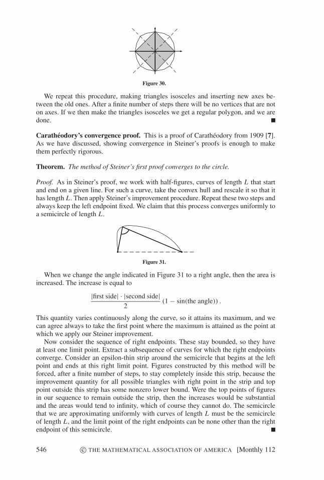
Figure 30.

We repeat this procedure, making triangles isosceles and inserting new axes be-tween the old ones. After a finite number of steps there will be no vertices that are noton axes. If we then make the triangles isosceles we get a regular polygon, and we aredone.

Caratheodory’s convergence proof. This is a proof of Caratheodory from 1909 [7].As we have discussed, showing convergence in Steiner’s proofs is enough to makethem perfectly rigorous.

Theorem. The method of Steiner’s first proof converges to the circle.

Proof. As in Steiner’s proof, we work with half-figures, curves of length L that startand end on a given line. For such a curve, take the convex hull and rescale it so that ithas length L . Then apply Steiner’s improvement procedure. Repeat these two steps andalways keep the left endpoint fixed. We claim that this process converges uniformly toa semicircle of length L .

Figure 31.

When we change the angle indicated in Figure 31 to a right angle, then the area isincreased. The increase is equal to

|first side| · |second side|2

(1 − sin(the angle)) .

This quantity varies continuously along the curve, so it attains its maximum, and wecan agree always to take the first point where the maximum is attained as the point atwhich we apply our Steiner improvement.

Now consider the sequence of right endpoints. These stay bounded, so they haveat least one limit point. Extract a subsequence of curves for which the right endpointsconverge. Consider an epsilon-thin strip around the semicircle that begins at the leftpoint and ends at this right limit point. Figures constructed by this method will beforced, after a finite number of steps, to stay completely inside this strip, because theimprovement quantity for all possible triangles with right point in the strip and toppoint outside this strip has some nonzero lower bound. Were the top points of figuresin our sequence to remain outside the strip, then the increases would be substantialand the areas would tend to infinity, which of course they cannot do. The semicirclethat we are approximating uniformly with curves of length L must be the semicircleof length L , and the limit point of the right endpoints can be none other than the rightendpoint of this semicircle.


Study’s convergence proof. This is a proof of Study from 1909 [7]. Again, it uses alimiting argument to get rid of the existence assumption.

Theorem. All areas of perimeter L are bounded by that of the circle with perimeter L.

Proof. From any figure, we create a sequence of isoperimetric figures with increasingareas that converges to the circle. We begin with a figure, that, as usual, we makeconvex and symmetric with respect to the x- and y-axes, leaving the area at least aslarge. The idea is to introduce further symmetry axes. Consider the part of the figure inthe first quadrant. The line that goes through the origin at angle of π/4 with the x-axisdoes not, in general, cut this perimeter in half. Translate it then, so that it does, in fact,cut the perimeter in half (Figure 32). Consider the two pieces that result:

Figure 32.

Both of these pieces could be used to make a figure with the same perimeter—justput the pointy end at the origin and reflect all the way around. So we take the piece withgreater area and do precisely this. Clearly, we have increased the area, or possibly left itthe same, and kept the perimeter fixed. We now have four symmetry axes. Continuingin the same way poses no difficulties, giving 2n+1 symmetry axes at the nth step.

Now to show convergence. Consider the points where the nth figure intersects thesymmetry axes. These lie on two circles (Figure 33):

Figure 33.

These circles remain within some closed disc. From the sequence of figures extract asubsequence for which the sequences of these circles converge. They must convergeto the same limit circle, for the distance between the circles at stage n is bounded bythe length of the slices of the figure’s perimeter, which is equal to 2−n−2 times the


perimeter. But when the circles converge to the same limit circle, the figures convergeuniformly to this circle as well. Therefore the limit circle can be none other than thecircle with the same perimeter as the figures. And so the increasing sequence of areasconverges to what must be their upper bound, the area of the circle.

6. VECTORS.

Gromov’s vector analysis proof. The paper [21] contains a nice two-dimensionaladaptation of the n-dimensional proof of Gromov from 1986 [16], which we now lookat. To set it up we consider a flaky physical-intuitive argument. Where the earth isperfectly spherical, we can balance a stick by placing it perpendicular to the ground.Where the earth is not spherical, say on the side of a hill, placing a stick perpendicularto the ground will cause it to tip over. Let’s agree that this experience convinces usthat, if we were stranded on a nonspherical planet, we could always find spots whereputting a stick perpendicular to the ground would cause it to tip over. Thus it is onlyfor the sphere that gravity always acts in the direction of the normal to the surface.Let’s also agree that this still holds when the universe is flat—when planets are planefigures.

To capture the mathematics of gravity, we should think of this in terms of vectorfields, and to make it easier for us we consider the negative of the gravitational field—just take the ordinary gravitational field and multiply the vectors by −1, pretendingthat we are in a dual universe where gravity pushes rather than pulls. Now take allfigures with a given area and fill them with cement. Then they all produce the sameamount of negative gravity. This negative gravity has flow lines out of the figure, butonly for the circle do they always flow out along the normal. For any other figure, thelines flow out askew, which we feel is an inefficient use of perimeter. So, perhaps, thiswill force the perimeter to be greater than that of the circle of the same area.

How do we exploit these ideas to make a proof? Well, the amount of negative gravitybeing produced can be calculated by summing over the boundary ∂ D of the figure Dthe outward flow ∂ F/∂�ν along the normal:∫

∂ D

∂ F

∂�ν ds.

We wish to show that a noncircular figure spreads the outflow over a greater perimeter.This would follow at once if we could show that the flow along the normal from a pointon a circle is greater than the flow along the normal from any point on the boundary ofany figure of the same area. That would mean that not only does a noncircular figuredilute the outflow at some places but also that it cannot concentrate the flow somewhereelse. Indeed, this is the case, as we are about to show by calculation.

Fix a point on the boundary and its normal (Figure 34):

Figure 34.

We now have a given area to distribute under this point to make the negative gravita-tional flow in the direction of the normal as large as possible. What will an arbitraryinfinitesimal square (Figure 35) contribute to the flow if we choose to include it?


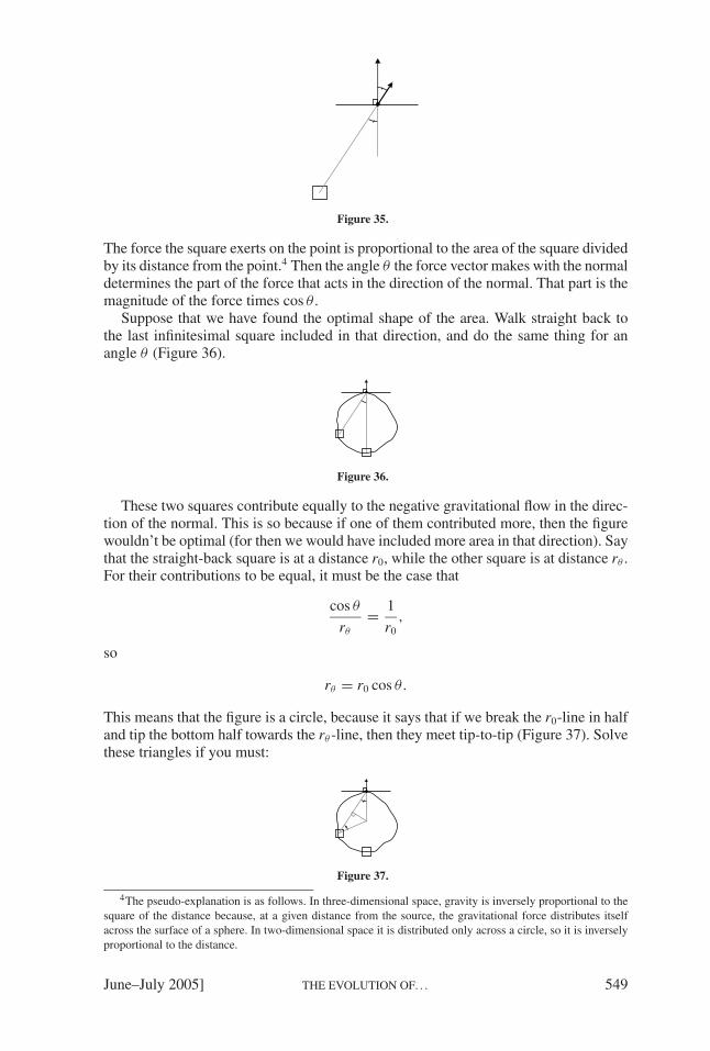
Figure 35.

The force the square exerts on the point is proportional to the area of the square dividedby its distance from the point.4 Then the angle θ the force vector makes with the normaldetermines the part of the force that acts in the direction of the normal. That part is themagnitude of the force times cos θ .

Suppose that we have found the optimal shape of the area. Walk straight back tothe last infinitesimal square included in that direction, and do the same thing for anangle θ (Figure 36).

Figure 36.

These two squares contribute equally to the negative gravitational flow in the direc-tion of the normal. This is so because if one of them contributed more, then the figurewouldn’t be optimal (for then we would have included more area in that direction). Saythat the straight-back square is at a distance r0, while the other square is at distance rθ .For their contributions to be equal, it must be the case that

cos θ

rθ

= 1

r0,

so

rθ = r0 cos θ.

This means that the figure is a circle, because it says that if we break the r0-line in halfand tip the bottom half towards the rθ -line, then they meet tip-to-tip (Figure 37). Solvethese triangles if you must:

Figure 37.

4The pseudo-explanation is as follows. In three-dimensional space, gravity is inversely proportional to thesquare of the distance because, at a given distance from the source, the gravitational force distributes itselfacross the surface of a sphere. In two-dimensional space it is distributed only across a circle, so it is inverselyproportional to the distance.


That’s it, we’re done. Since we got so carried away that we forgot to put the proofin a proper proof environment, we summarize it here.

Theorem. Of all figures with a given area, the circle has the shortest perimeter.

Proof. Consider the collection of all figures D with a given area. Fill each with nega-tive cement. Then they all generate the same amount of negative gravitational flow outthrough the boundary ∂ D of D (i.e., the integral

∫∂ D

∂ F

∂�ν ds

is the same for all of them). But the integrand is uniquely maximized by the circle, soall other figures must have greater perimeter.

Schmidt’s projection proof. This is a two-dimensional version of the n-dimensionalproof of Schmidt from 1939 [32]. The following is a physical analogy vaguely con-nected with this proof. Tape pins on a balloon so that they point perpendicularly out-ward from the surface. When the balloon is not inflated it is all wobbly, and the pinspoint in whatever direction they please. But when we inflate it, then the pins all pointaway from the center of the balloon. Similarly, it is because the circle is so packed witharea that its normals are forced to point away from its midpoint.

Theorem. L2 − 4π A ≥ 0, with equality only for the circle.

Proof. Begin with an arbitrary figure and parameterize the boundary by arclengtht �→ (x(t), y(t)) (i.e., use a unit speed parameterization, one with x2 + y2 = 1). Con-struct a circle that is as wide as the figure and project the boundary vertically onto it,as in Figure 38:

Figure 38.

Under this projection the x-coordinate is kept fixed and the y-coordinate is sent to, say,y, in a way that puts (x, y) on the circle. As (x, y) traces out our figure, the vector fromO to (x, y) points to the projection of (x, y) on the circle. The key insight is now that ifthe figure is a circle, then its normal is always parallel to (x, y), but if it is not a circle,then its normal is not always parallel to (x, y). In other words, the circle maximizesthe projection of (x, y) onto the normal (y,−x). Aha, a maximization property of the


circle! Looks like we’re on to something. To formalize this, we take the inner productof (x, y) and the normal (y,−x). This is less than the product of the lengths

x y − y x ≤ r,

and our geometric intuition tells us that equality occurs pointwise only for the circle.Let’s see what we can do with that. We have

A =∫ L

0x y dt ≤

∫ L

0r + y x dt.

The integral in the first term is of course just Lr , and the second integral is the negativearea of the circle. Now we are just one ad hoc factorization away from the isoperimetricinequality:

A ≤ Lr − πr 2 = L2

4π− π

4

(L

π− 2r

)2

≤ L2

4π.

7. DISSECTION.

Lawlor’s dissection proof. If you are getting tired of physical analogies, then skipahead, because this will be our most far-fetched one yet. If not, imagine a pizza. Theisoperimetric theorem says that the circular shape of pizzas maximizes the topping-to-crust ratio. We bake a noncircular pizza with the same amount of crust as a round one,and now we wish to show that less topping fits on this one. A naive attempt would beto slice the round pizza into slices in the customary manner, although perhaps thinner,and then to arrange these slices so that their crusts cover the crust of the noncircularpizza. The isoperimetric theorem would follow if the interior of the noncircular pizzawere always completely covered in the process. This will obviously not be so, but theidea is not beyond salvation. We will sense its spirit in the following proof of Lawlorfrom 1998 [26].

We restrict ourselves to polygons, by approximation, and also to quarter figures.This is alright because, given any figure, we can easily create a figure with the sameperimeter and at least as large an area that is symmetric with respect to the x- andy-axes. Specifically, draw a horizontal line that cuts the perimeter in half. Take asthe new figure the half with the greater area together with its reflection. Next, draw avertical line that cuts the new perimeter in half. Again, take as the new figure the halfwith the greater area together with its reflection.

Theorem. Among all fixed-length, equilateral n-gon arcs in the first quadrant, theregular one encloses the greatest area.

Proof. We cover our figure with triangles. We triangulate the regular n-gon arc bydrawing rays from the vertices to the origin:

Figure 39.


For the general case, we draw the same rays, only translated to start at the vertices.

Figure 40.

This gives us triangles that cover our figure, perhaps with excess and overlap, as shownin Figure 40. The picture contains the idea. Formally, convexity ensures that no ray cansneak under the preceding ray. As for covering, a point in the interior will be to theleft of the arc and between the first and last rays (those that are parallel to the axes),and thus it will be trapped between two consecutive rays and covered by the associatedtriangle.

By construction, all these triangles have the same base and the same opposite angle,and among such triangles the isosceles triangle has the greatest area. So the regularn-gon is greater piece by piece, and thus greater as a whole.

8. SERIES. The series approaches that follow are not very enlightening, but they dosuggest a systematic scheme for attacking inequalities:

Generic inequality. This + that ≥ 0, with equality when so-and-so.

Generic proof. Express the terms analytically and expand in series. Prove the inequal-ity by comparing coefficients—the point is that this is now essentially a matter ofarithmetic. Force equality and see what that means for the series.

Hurwitz [22], in the opening paragraph of the article containing his Fourier analysisproof, also tries to explain to us why a series approach is natural:

Fourier series and analogous expansions intervene quite naturally in the general theory ofcurves and surfaces. Indeed, this theory, conceived from the point of view of analysis, ob-viously deals with the study of arbitrary functions. I was thus led to apply Fourier series tosome geometric problems, and I obtained in this way some results which will be presented inthis work. It will be noticed that my considerations hardly form but a beginning in a certaindirection of research, which undoubtedly will give many new results.

Hurwitz’s Fourier series proof. This is the proof of Hurwitz from 1902 [22]. Firstwe address a couple of notational issues. We use old-school notation for Fourier series:

f (t) = 1

2a0 +

∞∑n=1

an cos nt + bn sin nt.

With this notation Parseval’s theorem reads

1

π

∫ 2π

0f (x)g(x) dx = a0b0

2+

∞∑n=1

anbn + cndn.



Proof. Choose a parameterization t �→ (x(t), y(t)) that traces out a given curve oflength L in time 2π with constant speed. This translates to

x2 + y2 =(

L

2π

)2

.

Let the Fourier series of the coordinate functions be

x(t) = 1

2a0 +

∞∑n=1

an cos nt + bn sin nt,

y(t) = 1

2c0 +

∞∑n=1

cn cos nt + dn sin nt.

Then the Fourier series for the derivatives are

x(t) =∞∑

n=1

n(bn cos nt − an sin nt),

y(t) =∞∑

n=1

n(dn cos nt − cn sin nt).

Next we use Parseval’s theorem to express L2 and A in terms of these coefficients.

L2 = 4π2

(L

2π

)2

= 2π2

(1

π

∫ 2π

0

(L

2π

)2

dt

)= 2π2

(1

π

∫ 2π

0x2 + y2 dt

)

= 2π2

( ∞∑n=1

n2(a2n + b2

n + c2n + d2

n )

),

A =∫ 2π

0x y dt = π

∞∑n=1

n(andn − bncn).

We hope that the isoperimetric inequality will follow when we combine these expres-sions. It does, as follows:

L2 − 4π A = 2π2

( ∞∑n=1

n2(a2n + b2

n + c2n + d2

n ) − 2n(andn − bncn)

)

= 2π2

( ∞∑n=1

(nan − dn)2 + (nbn + cn)

2 + (n2 − 1)(c2n + d2

n )

)

≥ 0.

When is there equality? Looking at the term for n = 1 we get

a1 = d1, b1 = −c1.


For all larger n the coefficients vanish

an = bn = cn = dn = 0,

that is,

x(t) = 1

2a0 + a1 cos t + b1 sin t,

y(t) = 1

2c0 − b1 cos t + a1 sin t.

The curve described by these equations is a circle.

Fourier analysis is not indispensable for this proof. Hardy, Littlewood, and Polya[17, pp. 186–187] manage without it, but as they say themselves:

The proof is in principle that of Hurwitz, but differs (a) in that we do not use the theory ofFourier series and (b) in our unsymmetrical treatment of x and y.

We could suggest adding: (c) in that it lacks the aesthetic appeal of Fourier analysis.

Carleman’s power series proof. Of all conformal mappings of the (complex) plane,the linear fractional transformations are those that send circles to circles. That is, theypreserve the perfection of the circle while other conformal mappings smudge thingsup. We now map the unit circle conformally onto some (simply connected) figure. Ifthe figure is not a circle, we hope to use one of those smudging mappings to revealthe imperfection L2 − 4π A > 0. But if the figure is a circle, a linear fractional trans-formation will do, resulting in the preservation of “perfection” (i.e., L2 − 4π A = 0).To prove this, we resort to using power series. This is the proof of Carleman from1921 [8].5


Proof. Given a simple closed curve of finite length L , we map the unit disk onto itsinterior by a conformal mapping ϕ and express the length and area in terms of ϕ′. Bystandard formulas from complex analysis,

L =2π∫

0

|ϕ′(z)| dθ, A =2π∫

0

1∫0

|ϕ′(z)|2r dr dθ.

To be able to compare the power series of the two terms we consider a function ψ thatis analytic in the unit disk and satisfies ψ2 = ϕ′. Then ψ has a power series expansionabout the origin

ψ(z) =∞∑

n=0

anzn.

5Kraus [24] in 1932 gives exactly the same proof and says: “If the proof of the isoperimetric inequality hasalready been carried out in this way, then I have not been able to find it in the literature.”


Let bn = ana0 + an−1a1 + · · · + a0an , so that( ∞∑n=0

anzn

)( ∞∑n=0

anzn

)=

∞∑n=0

bnzn.

Then

L =2π∫

0

|ψ2(z)| dθ = 2π

∞∑n=0

|an|2,

A =2π∫

0

1∫0

|ψ2(z)|2r dr dθ =2π∫

0

1∫0

|bn|2r 2n+1 dr dθ

= π

∞∑n=0

|bn|2n + 1

.

The isoperimetric inequality becomes

∞∑n=0

|bn|2n + 1

≤( ∞∑

n=0

|an|2)( ∞∑

n=0

|an|2)

,

and we can prove it by making termwise comparisons and invoking Cauchy’s inequal-ity:

|bn|2 = |ana0 + an−1a1 + · · · + a0an|2≤ (|an|2|a0|2 + |an−1|2|a1|2 + · · · + |a0|2|an|2

)(n + 1).

Equality occurs when

|ana0 + an−1a1 + · · · + a0an|2= (|an|2|a0|2 + |an−1|2|a1|2 + · · · + |a0|2|an|2

)(n + 1),

that is, when all the terms in the sum ana0 + an−1a1 + · · · + a0an are equal for all n.This means that {an} is a geometric sequence, say with ratio q. The consequence forϕ′ is that

ϕ′(z) = ψ(z)2 = a20

(1 − qz)2,

which we recognize as the derivative of a linear fractional transformation. So anarea maximizing curve is the image of the unit circle under a linear fractionaltransformation—a circle.

9. CONVEXITY. Here’s what we’re going to do. We take an arbitrary noncircularfigure. We manipulate it with clever reflections and things to get a nonconvex figureof the same area and perimeter. A nonconvex figure cannot have maximal area, so wewill then have shown that no noncircular figure can have the maximal area.


Convexity and symmetry. I saw this proof in [21]. Its origin is apparently unclear.

Theorem. If there is a smooth solution to the isoperimetric problem, then it is a circle.

Proof. Take a smooth solution. Place it so that the x-axis cuts the perimeter in half.Make a new figure from each half by combining it with its reflection in the x-axis. Eachof these two new figures must have the maximal area as well, for together they havetwice the maximal area and neither can have more than maximal area. Since they havemaximal area, they must be convex. Therefore, the x-axis must have cut the originalfigure at right angles, for otherwise one of our new figures would have a dent there(Figure 41).

Figure 41.

Take the new figures and repeat the process, only this time split the perimeter withthe y-axis instead. This gives four, still smooth, figures with maximal area that aresymmetric in both the x- and y-axes. Because of this symmetry, any line through theorigin cuts the perimeters of these figures in half, as demonstrated in Figure 42.

Figure 42.

Therefore, any line through the origin must meet each of the four figures (whenplaced with their “centers” at the the origin) at right angles. Otherwise, by reflectingthe halves we would again obtain a dented figure with maximal area. We conclude thatthe figures are all circles, so we must have had a circle to begin with.

Convexity and tangents. Here is a more general but less clean convexity proof ofDemar from 1975 [9].

Theorem. If there is a solution to the isoperimetric problem, then it is a circle.

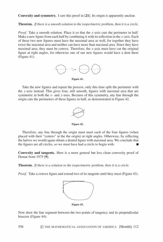
Proof. Take a convex figure and extend two of its tangents until they meet (Figure 43).

Figure 43.

Now draw the line segment between the two points of tangency and its perpendicularbisector (Figure 44):


Figure 44.

For the figure to have maximal area, the tangents must meet on this perpendicular line,for otherwise we could make a nonconvex figure with maximal area by reflecting thecut-off piece in it (Figure 45):

Figure 45.

This construction rules out many figures as candidates for maximal area. In par-ticular, it rules out all figures with any straight segments, for if one of our points oftangency were on such a segment, we could move it a little bit, causing a change inthe perpendicular bisector, while the tangent would still be the same, so the tangentscould not always meet on the perpendicular.

The foregoing construction also demonstrates that if we have the figure with themaximal area, then the tangents meet on this line and are of equal length. Moreover,this also holds for the normals at the points of tangency (Figure 46):

Figure 46.

We now wish to pick a third, arbitrary point on the boundary and show that it andthe two points of tangency are on a circle. For the construction to work, we cannot pickthis new point completely arbitrarily, however. The solution curve must have a tangentat this point. This is not a problem, since there is a dense set of points on the curve atwhich it has tangents (only nonconvexity could mess that up). Also, the tangent cannotbe parallel to the two tangents we have already. This is not a problem either, since thiscan happen only at isolated points now that we have ruled out figures with straightsegments.

With our new, third point, the situation looks something like Figure 47:

Figure 47.


The important thing is that the normals form a triangle that we now prove is not atriangle at all, but a point. We have just shown that the normals are pairwise equal:

Figure 48.

We combine the first two of these relations to get

=

Subtracting this from the third relation gives

− =

The conclusion: one side is the sum of the other two, so the triangle is not a propertriangle, and it is certainly not a line, so it must in fact be a point. It follows that allthree points are equidistant from this point, and therefore they lie on a circle.

10. PARALLEL CURVES. Take a convex figure and roll a circle along its boundary.The curve that is traced out by the center of the circle is what we call a parallel curve(Figure 49).

Figure 49.

Or, if you prefer, dip the circle in paint and have it bounce around with its midpointtrapped inside the figure. It will then paint the inside of the parallel figure.

The beautiful thing about parallel curves is that they preserve the quantity L2 − 4π A.The isoperimetric inequality L2 − 4π A ≥ 0 suggests that we think of L2 − 4π A asa quantity that shows how far the figure is from being a circle. Then a parallel figureis as far from being a circle as the original figure. Intuitively, we feel that this is onlynatural, since taking the parallel curve means, in a sense, “adding a circle” (and forcircles we have L2 − 4π A = 0).

Let’s establish the preservation of L2 − 4π A. For the rest of this section we will,for the sake of simplicity, deal only with parallel curves of convex polygons. So take aconvex polygon and construct the parallel curve using a circle of radius r (Figure 50).

Figure 50.


The new area is the old area plus the area of the strips plus the area of the shadedpieces. This is all easy to calculate once we realize that the shaded pieces fit togetherto form a disk. This is so because the sum of the angles of the shaded pieces is theamount by which we turn when we walk around the figure once (Figure 51).

Figure 51.

The preservation of L2 − 4π A is now easy to verify, for we have the relations be-tween the old area a and perimeter l and their new counterparts A and L:

A = a + lr + r 2π, L = l + 2πr,

giving

L2 − 4π A = l2 + 4lπr + 4π2r 2 − 4πa − 4πlr − 4π2r 2 = l2 − 4πa.

This preservation of L2 − 4π A seems like a good thing when our aim is to prove theisoperimetric inequality, but outer parallel curves are not of much use. What we reallyneed is inner parallel curves, which essentially allow us to move inwards until the areais exhausted, for then surely L2 − 4π A ≥ 0.

We consider two ways of setting this up. First, we come up with a contrived defini-tion of inner parallel curves, ensuring that they, too, magically preserve L2 − 4π A.We also give a more straightforward definition of inner parallel curves for whichL2 − 4π A is not preserved. Nevertheless, this new definition gets the job done.

Parallel curves with a twist. One way to think about outer parallel curves is this: theparallel curve is traced out by a moving normal, and when we reach a corner we letthe normal turn continuously to its new direction (Figure 52).

Figure 52.

We can do the same thing with an inward-pointing normal (Figure 53).

Figure 53.

Now see how clever we have been. We decide that the perimeter along the circulararcs should be counted negatively, and so too the areas they bound. (This makes somesense in terms of orientation.) Then the new area a and perimeter l will be

a = A − Lr + r 2π, l = L − 2πr.


We have thus managed to preserve L2 − 4π A:

l2 − 4πa = L2 − 4Lπr + 4π2r 2 − 4π A + 4π Lr − 4π2r 2 = L2 − 4π A.

We can now prove the isoperimetric inequality by taking any polygon and showingthat L2 − 4π A ≥ 0 for one of its parallel curves. We imagine taking inner parallelcurves further and further in until the area has shrunken to nothing. For a square, forinstance, we should use a normal of half the side length to trace out the parallel curve(Figure 54).

Figure 54.

There is then no positive area left, so indeed L2 − 4π A ≥ 0. But the picture says more.The negative area we are left with is composed precisely of the pieces we would haveto take away from the square for it to become a circle. This works for any polygon thatcircumscribes a circle (Figure 55).

Figure 55.

But this pretty property is lost for polygons not circumscribing circles (Figure 56).

Figure 56.

This figure is all messed up on the left: there is a little bit of twice negative area forinstance (three sides have swept past it). Nevertheless, it is still intuitively obvious thatwhen we take the inner parallel curve with an offset that is the radius of the greatestcircle we can inscribe, then we run out of positive area and get L2 − 4π A ≥ 0, as hasbeen proved, among others, by Bonnesen in 1921 [3], [4].

Parallel curves the no-nonsense way. For this approach we follow Bol’s article from1943 [2]. Bol is surprised that this “truly simple proof” has not been given earlier.

Theorem. L2 − 4π A ≥ 0 for convex polygons.

Proof. Given a convex polygon, we create parallel inner polygons by sliding all sidesperpendicularly inward. This process gives polygons of fewer and fewer sides, even-tually terminating in a point or a line (Figure 57).


Figure 57.

Points and lines have no area, hence for them the isoperimetric inequality is cer-tainly true. The idea is now to show that the quantity L2 − 4π A decreases as we moveinward. Then L2 − 4π A must have been nonnegative to begin with, because we makeit smaller and smaller and still end up with something nonnegative.

We illustrate the procedure in a case where the number of sides is reduced in orderto stress that the reasoning is always the same. Let’s say that the perimeters are L forthe big polygon and l for the small one, and that we have moved the sides inward by r(Figure 58).

Figure 58.

The big area A is the small area a plus the area of the strips lr plus the area of theshaded pieces. As before, we see that the shaded pieces fit together, but this time toform something like the shape in Figure 59:

Figure 59.

The spokes are equally long—they have length r—so we are dealing with an in-scribed circle. Inspired by that, we write r 2π for the area, where π must be slightlylarger than π . This means that the perimeter is 2r π , because the area is r times theperimeter divided by two (Figure 60),

=Figure 60.

as we see by summing the areas of the triangles in Figure 61:


Figure 61.

Now we have all we need to be able to tell what happens to L2 − 4π A, for we have

A = a + lr + r 2π , L = l + 2r π ,

which gives

L2 − 4π A = l2 + 4lr π + 4r 2π2 − 4πa − 4πlr − 4πr 2π

= l2 − 4πa + 4rl(π − π) + 4r 2π(π − π)

> l2 − 4πa,

confirming that this quantity decreases, as claimed.

11. INTEGRAL GEOMETRY. In prerevolutionary France, Georges Louis Leclerc,Comte de Buffon, spent his bourgeois leisure time tossing needles on the floor. In 1777he wrote ([5], quoted from [6, p. 473]):

I suppose that in a room in which the parquet floor is simply divided by parallel joints, onethrows a stick in the air and one of the players bets that the stick will not cross any of theparallels of the parquet floor, and that the other bets on the contrary that the stick will crosssome of these parallels; the chances of these two players are asked for.

Santalo’s integral geometry proof. This is a proof of Santalo [31, pp. 37–38].

Theorem. L2 − 4π A ≥ 0.

Proof. Consider a convex figure D of perimeter L . Now, instead of throwing needlesat it, throw circles. And use circles of the same perimeter as D (i.e., with radiusr = L/2π ; see Figure 62, where D is the figure with the boldface boundary).

Figure 62.

We hope that this will give us information about the area of D—the more circles inter-sect it the greater its area—and we capture this intuition by considering the weightedarea of the plane, ∫∫

R2

I (x, y) dx dy,


where we determine the weight I (x, y) of an infinitesimal square by putting the centerof one of our circles there and counting how many times it intersects the boundary∂ D of D. (One pesky detail is that the intersection-counting function I (x, y) might beinfinite at some points, but of course it will be so almost nowhere, so this cannot hurtthe integral.)

An approximation to this weighted area immediately occurs to those who paid care-ful attention when reading the last section. Only the region at most r away from D isgiven nonzero weight, that is, the area of the region Dr inside the outer parallel curveat distance r from D. This is, as we recall, A + Lr + r 2π . Also, if we drop one ofour circles with its center anywhere inside this parallel figure, then it will intersect theboundary of D at least twice (there will be no zero-area in the middle, for the circlecannot fit inside the figure). In terms of formulas,

∫∫R2

I (x, y) dx dy ≥∫∫

Dr

2 dx dy = 2(A + Lr + r 2π

).

Now we calculate the weighted area by brute force. Consider a point on ∂ D. Whichcircles intersect this point? They are, of course, the circles with centers at distance rfrom it (Figure 63).

Figure 63.

Consider an infinitesimal ds-segment of ∂ D. Which circles intersect this segment?They must be circles with centers that lie in two strips like those in Figure 64:

Figure 64.

The strips have height 2r (in the direction perpendicular to the boundary segmentds) and constant width ds, so the ds-segment contributes a total amount of weightedarea 4rds. Summing these contributions we obtain

∫∫R2

I (x, y) dx dy =∫∂ D

4rds = 4r L .

We now have two expressions for the weighted area that we can combine,

4r L ≥ 2(

A + Lr + r 2π),

and, remembering that we chose r = L/2π , this reduces to the isoperimetric inequal-ity.


There is more to be extracted from these ideas. We write An for the area with weightn, giving a total weighted area of

A1 + 2A2 + 3A3 + · · · ,although all the odd terms will be zero of course (almost any circle intersects ∂ D aneven number of times). We have just calculated the total weighted area to be 4r L , fromwhich we conclude that

4r L = 2A2 + 4A4 + 6A6 + · · · .And the area inside the parallel curve consists of all the areas with nonzero weight,

A + r L + r 2π = A2 + A4 + A6 + · · · .Taking half the first of these equations and subtracting the second gives

r L − A − r 2π = A4 + 2A6 + 3A8 + · · · .Since r = L/2π , this gives us an expression for L2 − 4π A in terms of weighted areas:

L2 − 4π A ≥ 4π (A4 + 2A6 + 3A8 + · · ·) .

Now we see that there can be equality only for the circle, for that’s the only casewhere there is no four-area A4. We can see this as follows. Place a circle on D asshown in Figure 65:

Figure 65.

Slide the circle along ∂ D, always keeping just a little bit of it outside. For there to beno four-area, the other side of the circle must never hit ∂ D. This works when D andthe circle are the same, or when D contains the circle, which is of course impossible.

We have done our best to stay clear of generalizations of the isoperimetric theorem,but we cannot resist the temptation to mention one pretty generalization connectedwith this proof, a generalization that is also important for understanding much of theisoperimetric literature. Recall one of our definitions of parallel curves: we took acircle, dipped it in paint, and moved it about with its midpoint inside a figure in or-der to paint the parallel figure. Obviously, we could generalize this procedure, takingsomething other than the circle as our brush. We could then take any point in its inte-rior to be the point that is not allowed to leave the figure. Nor are we allowed to twistthe brush. The result is what is known as Minkowski addition. The behavior of thisprocedure is captured by the Minkowski inequality:√

painted area ≥ √area of the figure + √

area of the brush.

If we choose the brush to be a circle, then this inequality asserts that√area inside the parallel curve ≥ √

area of the figure + √area of the circle,

and it readily reduces to the isoperimetric inequality. The most beautiful proof of theMinkowski inequality that I know of is a very natural generalization of the proof wehave given here—we just drop this brush figure instead of the circle and everythingworks out. A very readable exposition of this proof is found in [12].


REFERENCES

1. W. Blaschke, Kreis und Kugel, 1916; reprinted by Chelsea, New York, 1949.2. G. Bol, Einfache Isoperimetriebeweise fur Kreis und Kugel, Abh. Math. Sem. Univ. Hamburg 15 (1943)

27–36.3. T. Bonnesen, Uber eine Verscharfung der isoperimetrischen Ungleichheit des Kreises in der Ebene und

auf der Kugeloberflache nebst einer Anwendung auf eine Minkowskische Ungleichheit fur konvexeKorper, Math. Annalen 84 (1921) 216–227.

4. , Les problemes des isoperimetres et des isepiphanes, Gauthier-Villars & Cie, Paris, 1929.5. G. Buffon, Essai d’arithmetique morale, 1777.6. , Œuvres philosophiques de Buffon, Presses universitaires de France, Paris, 1954.7. C. Caratheodory and E. Study, Zwei Beweise des Satzes, daß der Kreis unter allen Figuren gleichen

Umfanges den großten Inhalt hat, Math. Annalen 68 (1909) 133–140.8. T. Carleman, Zur Theorie der Minimalflachen, Math. Z. 9 (1921) 154–160.9. R. F. Demar, A simple approach to isoperimetric problems in the plane, Math. Mag. 48 (1975) 1–12.

10. F. Edler, Vervollstandigung der Steinerschen elementargeometrischen Beweise fur den Satz, daß derKreis grosseren Flacheninhalt besitzt, als jede andere ebene Figur gleich grossen Umfanges, Nachrichtenvon der Konigl. Gesellschaft der Wissenschaften und der Georg-Augusts-Universitat zu Gottingen (1882)73–80.

11. L. Euler, Methodus inveniendi lineas curvas maximi minimive proprietate gaudentes sive solutio prob-lematis isoperimetrici latissimo sensu accepti, 1744, German translation in [34].

12. H. Flanders, A proof of Minkowski’s inequality for convex curves, this MONTHLY 75 (1968) 581–593.13. G. Galilei, Discorsi e dimostrazioni matematiche intorno a due nuove scienze, Elsevier Press, Leiden,

1638.14. S. Gandz, Isoperimetric problems and the origin of quadratic equations, Isis 32 (1940) 103–115.15. C. F. Geiser, Zur Erinnerung an Jakob Steiner, Verhandlungen der Schweizerischen Naturforschenden

Gesellschaft 56 (1874) 215–251.16. M. Gromov, Isoperimetric inequalities in Riemannian manifolds, 1986, appendix in [28].17. G. H. Hardy, J. E. Littlewood, and G. Polya, Inequalities, Cambridge University Press, Cambridge,

1934.18. T. L. Heath, A History of Greek Mathematics, vol. 2, Clarendon Press, Oxford, 1921.19. D. Hilbert, Mathematische Probleme. Nachrichten von der Koniglichen Gesellschaft der Wissenschaften

zu Gottingen (1900) 253–297; English translation in [20].20. , Mathematical problems, Bull. Amer. Math. Soc. 8 (1902) 437–479.21. H. Howards, M. Hutchings, and F. Morgan, The isoperimetric problem on surfaces, this MONTHLY 106

(1999) 430–439.22. A. Hurwitz, Sur quelques applications geometriques des series de Fourier, Annales Scientifiques de

l’Ecole Normale Superieure 19 (1902) 357–408.23. Morris Kline, Mathematics for the Nonmathematician, Dover, New York, 1985.24. W. Kraus, Uber den Zusammenhang einiger Charakteristiken eines einfach zusammenhangenden Bere-

iches mit der Kreisabbildung, Mitt. Math. Sem. Giessen 21 (1932) 1–28.25. J. L. Lagrange, Essai d’une nouvelle methode pour determiner les maxima et les minima des formules

integrales indefinies., Miscellanea Philosophica-Mathematica Societatis Privatae Taurinensis 2 (1762)173–195; German translation in [35].

26. G. Lawlor, A new area maximization proof for the circle, Math. Intelligencer 20 (1998) 29–31.27. S. Lhuilier, De relatione mutua capacitatis et terminorum figurarum etc, Warsaw, 1782.28. V. D. Milman and G. Schechtman, Asymptotic Theory of Finite Dimensional Normed Spaces, Lecture

Notes in Mathematics, no. 1200, Springer-Verlag, Berlin, 1986.29. G. R. Morrow, Proclus: A Commentary on the First Book of Euclid’s Elements, Princeton University

Press, Princeton, 1970.30. O. Perron, Zur Existenzfrage eines Maximums oder Minimums, Jahresber. Deutsch. Math.-Verein. 22

(1913) 140–144.31. L. Santalo, Introduction to Integral Geometry, Hermann & Cie, Paris, 1953.32. E. Schmidt, Uber das isoperimetrische Problem im Raum von n Dimensionen, Math. Z. 44 (1939) 689–

788.33. M. Spivak, A Comprehensive Introduction to Differential Geometry, vol. 4, 2nd ed., Publish or Perish,

Berkeley, CA, 1979.34. P. Stackel, Abhandlungen uber Variations-Rechnung. Erster Theil., vol. 46 of Ostwald’s Klassiker der

exakten Wissenschaften, Engelman, Leipzig, 1894.35. , Abhandlungen uber Variations-Rechnung. Zweiter Theil., vol. 47 of Ostwald’s Klassiker der

exakten Wissenschaften, Engelman, Leipzig, 1894.


36. J. Steiner, Einfache Beweise der isoperimetrischen Hauptsatze, J. Reine Angew. Math. 18 (1838) 281–296.

37. , Sur le maximum et le minimum des figures dans le plan, sur la sphere et dans l’espace engeneral. premier memoire, J. Reine Angew. Math. 24 (1842) 93–162.

38. , Sur le maximum et le minimum des figures dans le plan, sur la sphere et dans l’espace engeneral. second memoire, J. Reine Angew. Math. 24 (1842) 189–250.

39. , Gesammelte Werke, vol. 2, Berlin, 1882.40. I. Thomas, Selections Illustrating the History of Greek Mathematics, vol. 2, Harvard University Press,

Cambridge, 1941.41. G. J. Toomer, Ptolemy’s Almagest, Princeton University Press, Princeton, 1998.42. K. Weierstrass, Mathematische Werke, vol. 7, Mayer & Muller, Berlin, 1927.

VIKTOR BLASJO recently received his undergraduate degree from Stockholm University. Seeing his workwarmly received by the MONTHLY, he feels that perhaps there is a place in this world after all for a humblestudent who just wants to understand [email protected]

To August Ferdinand

If a circle you sendFrom the deserts of sandOf a land Oriental and Gobi-ous,With a circle you’ll end,As we now understand,Thanks to nonorientable MobiusThat umlaut is hard, and woe be us—We always misprOnounce your name.Ah, Mobius, Mobius, Mobius—You one-sided stripper of fame!

——Submitted by Seth Braver, University of Montana (Missoula)


the evolution of. . . the isoperimetric problem - mathematical

Documents