the evolutionary rationality of social learning -...
TRANSCRIPT
The Evolutionary Rationality of SocialLearning
Richard McElreath∗,1, Barbara Fasolo2, and Annika Wallin3
1Department of Anthropology and Graduate Groups in Ecology, PopulationBiology and Animal Behavior, University of California, Davis CA 95616, USA2Department of Management (Operational Research Group), London School of
Economics and Political Science, G313 Houghton Street, London WC2A 2AE UK3Department of Philosophy, Lund University, Kungshuset, Lundagard, 222 22
Lund SE
DraftJuly 21, 2009
Contents
1 Introduction 2
2 Social learning heuristics 42.1 The environmental challenge . . . . . . . . . . . . . . . . . . . 52.2 Individual updating . . . . . . . . . . . . . . . . . . . . . . . . 62.3 “Unbiased” social learning . . . . . . . . . . . . . . . . . . . . 62.4 Consensus social learning . . . . . . . . . . . . . . . . . . . . . 82.5 Payoff biased social learning . . . . . . . . . . . . . . . . . . . 92.6 Prestige bias . . . . . . . . . . . . . . . . . . . . . . . . . . . . 112.7 Kin preference . . . . . . . . . . . . . . . . . . . . . . . . . . . 12
∗Corresponding author. [email protected]
1
McElreath, Fasolo, Wallin Evolutionary Rationality of Social Learning
3 Ecological variation and social learning 153.1 Spatial variation in the environment . . . . . . . . . . . . . . . 16
3.1.1 Individual updating . . . . . . . . . . . . . . . . . . . . 173.1.2 Unbiased social learning . . . . . . . . . . . . . . . . . 173.1.3 Consensus social learning . . . . . . . . . . . . . . . . . 193.1.4 Payoff bias . . . . . . . . . . . . . . . . . . . . . . . . . 223.1.5 Summary . . . . . . . . . . . . . . . . . . . . . . . . . 23
3.2 Temporal variation . . . . . . . . . . . . . . . . . . . . . . . . 243.2.1 Temporal variation may favor randomized or mixed
strategies . . . . . . . . . . . . . . . . . . . . . . . . . 253.2.2 Consensus learning less favored under temporal variation 343.2.3 Summary . . . . . . . . . . . . . . . . . . . . . . . . . 35
4 Conclusion 38
1 Introduction
A common premise surrounding magic in human societies is that words (aswell as other symbols) themselves have power. Speaking the right words inthe right context is believed to create fantastic effects. This kind of belief isnot only a feature of western myth and magic—nearly everything from Norserunes to magic in the Harry Potter books requires activation with words—but also of African (famously of Azanda oracles: Evans-Pritchard 1937) andAsian (Daoist incantations) traditions. Some healers in the Muslim worldwrite verses from the Koran in ink, and then wash the ink into a potionto be consumed. In Swahili, one can use the word (dawa) to refer both tomagical spells and to the influence a charismatic speaker has over a crowd.
Why do so many peoples believe that words themselves are magical?These beliefs are not necessarily irrational. Every one of us, by speaking,can alter the minds of those within earshot. With the word snake, onecan conjure a (potentially terrifying) image in the minds of others, whoare almost entirely unable to resist. Statements like, “do not think of anelephant,” reveal how hard it is to really control our thoughts as well asthe potential power the mere utterances of others have over us. Of coursepeople are savvy and do not robotically obey all suggestion or command.However, spoken opinion and advice is highly valued almost everywhere. Thewords of others, carrying information, can have powerful effects on our own
2

McElreath, Fasolo, Wallin Evolutionary Rationality of Social Learning
behavior. The mere suggestion that something—like a measles vaccine—isdangerous can have huge effects on behavior. People and governments intuitthis power and as a result attempt to control the words they themselves andothers are exposed to. Words really are a kind of mind control, or at leastmind influence. Their power can travel through the empty air and affect thebehavior of masses of other people in powerful ways.
The psychology of humans is uniquely elaborated for this kind of “magi-cal” influence. The capacity for language is only one way that social influenceon behavior is truly baked into our nature. Observational learning of variouskinds is equally powerful, as people combine theory and social informationto arrive at inferences about the reasons for and consequences of behavior.But animals other than humans also use social information (e.g. Bonner 1980,Galef 1992, 1996, Price et al. 2009, Giraldeau and Caraco 2000, Fragaszy andPerry 2003, Laland and Galef 2009). While the psychological mechanismsand diversity of social learning heuristics among, for example, baboons isnot the same as that among humans, the savvy monkey too uses informationfrom its social environment. As a result, evolutionary ecology of humansand other animals has long been interested in the design and diversity ofsocial learning heuristics, simple strategies that animals use to extract usefulinformation from their social environments.
In this chapter, we review a slice of this literature, as well as explicitlyanalyze the evolution of social learning heuristics. We outline a family of so-cial learning heuristics and analyze their evolutionary performance—abilityto persist and replace other heuristics—under two broadly different kinds ofenvironmental variation. As each social learning heuristic also constructs asocial environment as individuals use it, we consider the population feed-backs of each heuristic, as well. This means that the analyses in this chapterare simultaneously ecological—the performance of each heuristic is alwaysin the context of a specific set of assumptions about the population struc-ture and environment—as well as game theoretic—social learning heuris-tics use but also modify the social environment, inducing strong frequency-dependence. Our analyses are also explicitly evolutionary—heuristics succeedor fail depending upon long-term survival and reproduction in a population,not atomistic one-shot payoffs. As a result, some of our conclusions reflectan evolutionary rationality that is sometimes counter-intuitive. For example,heuristics that randomize their behavior can succeed where those that areconsistent fail. Overall, however, the approach we review here supports thegeneral conclusion that social learning heuristics are likely to be multiple and
3

McElreath, Fasolo, Wallin Evolutionary Rationality of Social Learning
subtly adapted to different physical, statistical, and social environments.
2 Social learning heuristics
In parallel to the literature in bounded rationality, evolutionary ecologistsand anthropologists studying social learning have proposed that there ex-ists a toolbox of contextually deployed heuristics that are suited to differentecological and social environments (reviews in Henrich and McElreath 2003,Richerson and Boyd 2005). The basic premise is that information about theworld is costly to acquire and process (Boyd and Richerson 1985). Therefore,natural selection favors cognitive strategies that leverage the specific corre-lations of specific environments in order to make locally-adaptive choices.Each heuristic in the toolbox is best deployed in a different circumstance,and some heuristics are more domain-general than others. Thus the expecta-tion is an ecology of inferential strategies that individuals can use to choosebehavior. While some of these strategies are more cognitively demandingand information hungry than others, all are quite “bounded,” compared toBayesian justifications for social learning (Boyd and Richerson 2005, 2001,Bikhchandani et al. 1992). Like other hypothesized heuristics, these sociallearning heuristics can be compared to laboratory behavior (Efferson et al.2008, McElreath et al. 2008, 2005, Mesoudi and O’Brien 2008, Mesoudi andWhiten 2008, Mesoudi 2008).
In this section, we outline and begin to analyze a toolbox of social learningheuristics that evolutionary ecologists and evolutionary anthropologists havestudied. This collection of heuristics is not complete. Many other heuristicscould be nominated, and each heuristic we do nominate is in reality a familyof heuristics. However, by constraining our discussion to the most commonly-discussed strategies, we have space to derive each from first (or at least basic)principles and, later, analyze the performance of each in different ecologicalcircumstances.
We expect that people (and perhaps other animals) possess a toolbox ofsocial learning heuristics, built up from both basic innate learning strategiesas well as socially-transmitted and individually-learned heuristics. Thereforeour goal is to study the conditions, both in terms of physical and socialenvironment, that favor different heuristics. An empirical program that testsfor the use of these heuristics uses such considerations for predicting thekinds of experimental treatments in which different heuristics will be deployed
4

McElreath, Fasolo, Wallin Evolutionary Rationality of Social Learning
Table 1: Social learning heuristics discussed in this chapter, with other namesfor the same strategies and citations to a sample of previous evolutionaryanalysis.
Heuristic Other names CitationsUnbiasedsocial learning
Linear social learning, randomcopying, imitation
Boyd and Richerson (1995,1985), Cavalli-Sforza and Feld-man (1981), Rogers (1988),Mesoudi and Lycett (2009),Aoki et al. (2005), Wakanoet al. (2004)
Consensuslearning
Conformity, conformist trans-mission, positive frequency de-pendent imitation, majorityrule imitation
Boyd and Richerson (1985),Mesoudi and Lycett (2009),Lehmann and Feldman(2008), Henrich and Boyd(2001, 1998), Wakano andAoki (2007)
Payoff bias Success bias, indirect bias Boyd and Richerson (1985),Henrich (2001), Schlag (1998,1999)
Prestige bias Indirect bias Boyd and Richerson (1985),Henrich and Gil-White (2001)
Kin bias Vertical transmission, parent-child transmission
McElreath and Strimling(2008)
(McElreath et al. 2008, 2005). In Table 1, we list the social learning heuristicsthat we consider further in this chapter, also listing aliases and a sample ofrelevant citations to previous work.
2.1 The environmental challenge
In order to make progress defining and analyzing the performance of differentlearning heuristics, we have to define the challenge the organism faces. Herewe use an evolutionary framing of the common multi-armed bandit problem.
Assume that a each individual at some point in its life has to choosebetween a very large number of distinct behavioral options. These options
5
McElreath, Fasolo, Wallin Evolutionary Rationality of Social Learning
could be timing of reproduction, patterns of paternal care, or any other set ofmutually exclusive options. Only one of these options is optimal, producinga higher fitness benefit than all the others. In particular, we will assumethat a single optimal behavior increases an individual’s fitness by a factor1 + b > 1. All other behavior leaves fitness unchanged. In particular, let w0
be an individual’s fitness before behaving. Then those who choose optimallyhave fitness w0(1 + b), while those who do not have fitness w0. Becausefitness does not depend upon how many other individuals also choose thesame option, these payoff are not directly frequency dependent.
Since there are a very large number of alternative choices, randomly guess-ing will not yield a fitness payoff much greater than w0. It is possible to reachall the same conclusions in a two-option model (see e.g. Rogers 1988). Butby assuming the number of alternative choices is actually infinite, this willmake the mathematical analyses that follow much easier to complete and tounderstand.
2.2 Individual updating
The foil for all the social learning heuristics we consider here is a gloss indi-vidual updating heuristic. However the mechanism works in detail, we assumethat individuals have the option of relying exclusively on their own experi-ence, when deciding how to behave. We assume that individual updatingrequires sampling and processing effort, as well as potential trial-and-error.As a result, an organism that uses individual updating to learn optimal be-havior pays a fitness cost by having their survival multiplied by c ∈ [0, 1].This means the fitness of an individual updater is always w0(1 + b)c > 1. Weassume that individual updating is always successful at identifying optimalbehavior. We have analyzed the same set of heuristics, assuming that indi-vidual updating is successful only a fraction s of the time. This assumption,while biologically satisfying, adds little in terms of understanding. It changesnone of the qualitative results we will describe in later sections, while addingmathematical complexity. We decided to omit the s factor for the sake ofclarity only.
2.3 “Unbiased” social learning
Probably the simplest kind of social learning is a strategy that randomlyselects a single target to learn from. Much of the earliest evolutionary work
6
McElreath, Fasolo, Wallin Evolutionary Rationality of Social Learning
on social learning has considered this strategy (Cavalli-Sforza and Feldman1981, Boyd and Richerson 1985), and even more recent work continues tostudy its properties (Aoki et al. 2005, Wakano et al. 2004).
To formalize this heuristic, consider a strategy that, instead of trying toupdate individually, copies a random member of the previous generation.Such a strategy avoids the costs of learning, c. The drawback is that thepayoff from such a heuristic depends upon the quality of available socialinformation. We will refer to such a strategy as “unbiased” social learning.We use the word “unbiased” to describe this kind of social learning, althoughthe word “bias” is problematic. We use the term to refer only to deviationsfrom random, not from normative standards. The word “bias” has been usedin this way for some time in the evolutionary study of social learning (Boydand Richerson 1985, for example).
Let q (“quality” of social information) be the proportion of optimal be-havior among possible targets of social learning. Then the expected fitness ofan unbiased social learner is w0(1 + qb), wherein b is discounted by the prob-ability that the unbiased social learner acquires optimal behavior. Like othersocial learning heuristics, unbiased social learning actively constructs socialenvironments itself. As a result, a satisfactory analysis must be dynamic.We consider such an analysis in a later section.
Note that we assume no explicit sampling cost of social learning. Indeed,several of the social learning heuristics we consider in this chapter use thebehavior of more than one target, and we have not considered explicit costsof sampling these targets either. Consensus social learning (below), in oursimple model of it, uses three targets, and payoff biased social learning (laterin this section) uses two targets. Does this mean that consensus is worsethan payoff bias, when both are equal in all other regards? We think theanswer to this question will depend upon details we have not modeled. Doother activities provide ample opportunity to sample targets for social learn-ing or must individuals instead search them out and spend time observingtheir behavior? If the behavior in question is highly complex and requirestime and practice to successfully transmit, like how to make an arrow, thenconsensus learning may entail higher behavioral costs than, say, payoff bias.This is because a consensus learner needs to observe the detailed technique ofthree (or more) individuals, while the payoff biased learner must only observepayoffs and then invest time observing one target. We could invent storiesthat favor consensus, as well. And while constructing and formalizing suchstories is likely productive, it is a sufficiently detailed project that we have
7
McElreath, Fasolo, Wallin Evolutionary Rationality of Social Learning
not undertaken it in this chapter. But we do not wish to send the messagethat sampling costs and sampling strategy—how many to sample and whento stop, for example—are uninteresting or unimportant questions. They aresimply beyond the scope of this introduction.
2.4 Consensus social learning
An often discussed category of social learning heuristics are those that usethe commonality of an option as a cue (Boyd and Richerson 1985, Henrichand Boyd 1998, Mesoudi and Lycett 2009, Wakano and Aoki 2007). Whenan individual can sample more than two targets, it is possible to use thefrequency of observed options among the targets as a cue to guide choice.While three is the minimum number of sampled targets needed to use thiskind of heuristic, the larger the sample of targets, the more reliable theheuristic can be.
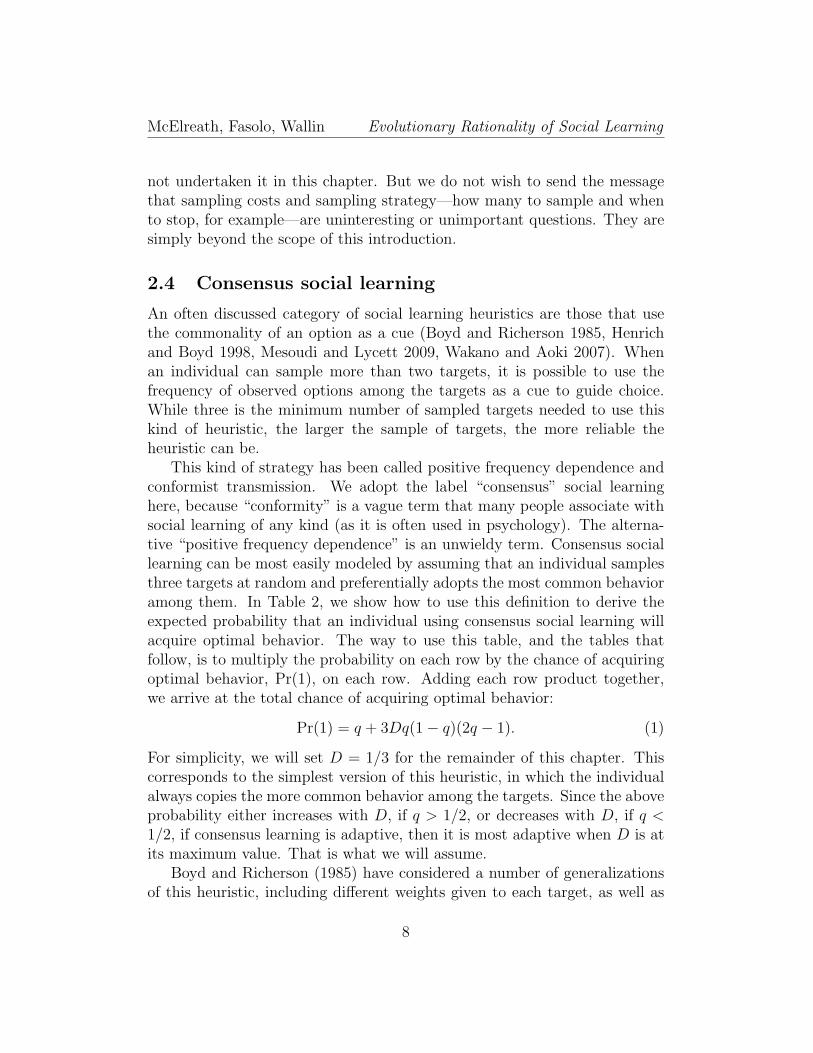
This kind of strategy has been called positive frequency dependence andconformist transmission. We adopt the label “consensus” social learninghere, because “conformity” is a vague term that many people associate withsocial learning of any kind (as it is often used in psychology). The alterna-tive “positive frequency dependence” is an unwieldy term. Consensus sociallearning can be most easily modeled by assuming that an individual samplesthree targets at random and preferentially adopts the most common behavioramong them. In Table 2, we show how to use this definition to derive theexpected probability that an individual using consensus social learning willacquire optimal behavior. The way to use this table, and the tables thatfollow, is to multiply the probability on each row by the chance of acquiringoptimal behavior, Pr(1), on each row. Adding each row product together,we arrive at the total chance of acquiring optimal behavior:
Pr(1) = q + 3Dq(1− q)(2q − 1). (1)
For simplicity, we will set D = 1/3 for the remainder of this chapter. Thiscorresponds to the simplest version of this heuristic, in which the individualalways copies the more common behavior among the targets. Since the aboveprobability either increases with D, if q > 1/2, or decreases with D, if q <1/2, if consensus learning is adaptive, then it is most adaptive when D is atits maximum value. That is what we will assume.
Boyd and Richerson (1985) have considered a number of generalizationsof this heuristic, including different weights given to each target, as well as
8
McElreath, Fasolo, Wallin Evolutionary Rationality of Social Learning
Table 2: Probabilities of acquiring optimal (1) and non-optimal (0) behavior,using a simple consensus social learning heuristic. D < 1/3 is the strength of thepreference for consensus. Like all later tables of this kind, one can use this tableto compute the chance of acquiring optimal behavior, using this heuristic. Thecolumns are, in order from left to right: the vector of observed behavior from asample of three targets, where 1 indicates optimal behavior and 0 any non-optimalbehavior; the probability of sampling that vector; the probability of acquiringoptimal behavior under the heuristic, given that sample; and the probability ofacquiring non-optimal behavior. First, multiply each probability of the observedvector of behavior by the probability of acquiring optimal behavior, Pr(1). Then,add together all the products from each row. In this case, q3 × 1 + 3q2(1 − q) ×(2/3 + D) + 3q(1− q)2 × (1/3−D) + (1− q)3 × 0 simplifies to Expression 1 in themain text.
Observed behavior Pr(Obs) Pr(1) Pr(0)1 1 1 q3 1 01 1 0 3q2(1− q) 2/3 +D 1/3−D1 0 0 3q(1− q)2 1/3−D 2/3 +D0 0 0 (1− q)3 0 1
correlations among the behavior of the targets. We will ignore these com-plications in this chapter, as our goal is to motivate a mode of analysis andto emphasize the differences among quite different social learning heuristics,rather than among variants of the same heuristics.
2.5 Payoff biased social learning
Another often analyzed category of social learning heuristic is payoff guidedlearning (Boyd and Richerson 1985, Schlag 1998, 1999, Stahl 2000). By com-paring observable payoffs—health, surviving offspring, or even more domain-specific measures of success—among targets, an individual can use differencesin payoff as a guide for learning. This kind of heuristic generates a dynamicoften called “the replicator dynamic” in evolutionary game theory (Gintis2000). This dynamic is very similar to that of natural selection, and is of-ten used as a boundedly-rational assumption in social evolutionary models(McElreath et al. 2003, e.g.) and even epidemiology (Bauch 2005).
A simple model of payoff biased social learning assumes that individuals
9
McElreath, Fasolo, Wallin Evolutionary Rationality of Social Learning
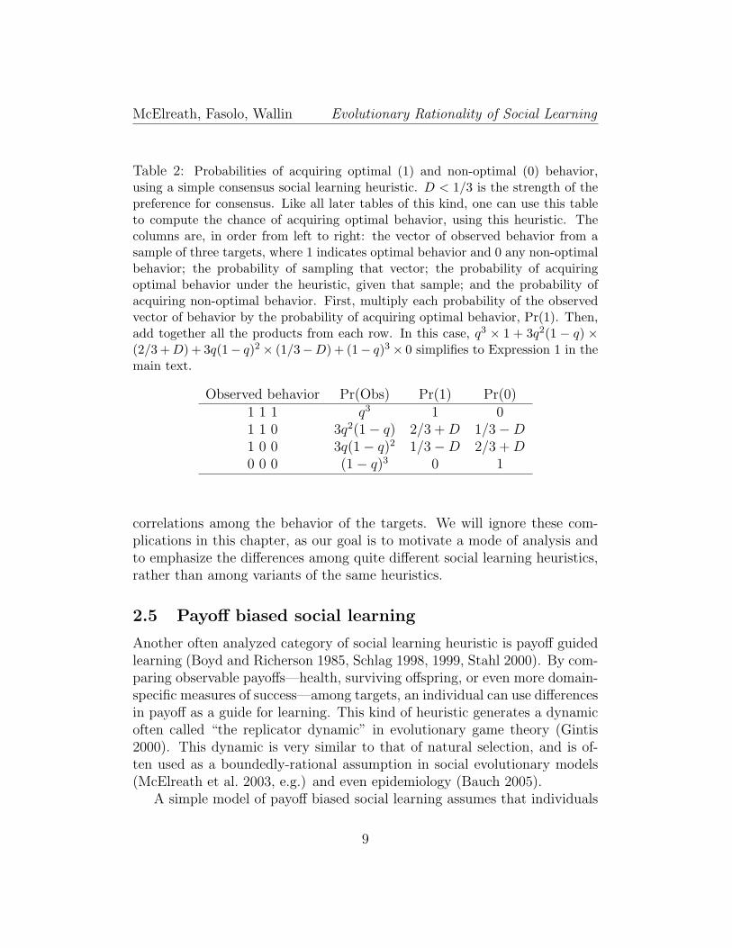
Table 3: Probabilities of acquiring optimal (1) and non-optimal (0) behavior,using payoff-biased social learning. In this table, q is the frequency of optimalbehavior among targets and x is the chance of incorrectly judging the payoff of atarget (or similarly, 1−x is the correlation between behavior and observed payoffs).The individual using payoff biased social learning samples two targets at randomand assesses their payoffs. If both targets have the same behavior, then errorsin judging payoffs are irrelevant. If instead one target has optimal behavior (1)and the other some non-optimal behavior (0), then errors matter. The individualcopies the behavior of the target with the higher observed payoff, unless bothobserved payoffs are the same, in which case one target is copied at random.
Actual behavior Pr(actual) Observed payoffs Pr(obs) Pr(1) Pr(0)1 1 q2 1 01 0 2q(1− q) 1 0 (1− x)2 1 0
0 0 x(1− x) 1/2 1/21 1 x(1− x) 1/2 1/20 1 x2 0 1
0 0 (1− q)2 0 1
sample two targets and preferentially adopt the behavior of the target withthe higher observed payoff. We assume that there is a chance x that theindividual can correctly judge the payoff of a target to be high or low. An-other interpretation is that x is the chance that a target’s observable payoffis uncorrelated with behavior. Using these assumptions, we show in Table 3that this heuristic leads to a chance:
Pr(1) = q + q(1− q)(1− x)
of acquiring optimal behavior.A more general model of payoff-bias allows for the aspect of the target to
be judged as “success” to itself be socially transmitted. When this is the case,many baroque social processes become possible, such as the exaggeration ofpreferences for traits that are judged as successful (Boyd and Richerson 1985).
10
McElreath, Fasolo, Wallin Evolutionary Rationality of Social Learning
2.6 Prestige bias
Suppose the cue that guides target choice is not observed success, but rathera social judgment of success. In many cases, individuals cannot have gatheredenough information personally to evaluate the success of models, and so someproxy will have to be used. Consider for example the task of judging whichhunters are the best (Hill and Kintigh 2009). Hunting returns are highlystochastic—even the best hunters usually come home with nothing. As aresult, figuring out who is a good hunter is a data-intensive task that evenanthropologists who weigh everything that comes back to camp have a hardtime addressing. Nevertheless, people in such societies often agree upon whoare the best hunters and data analysis (when we have it) supports theiropinion. How do they learn who is a good hunter?
One recurring idea is that social judgments of general success can be auseful guide. It may not be possible to individually learn who is a goodhunter, but it may be possible for individual hunters to accumulate prestigeor prestige objects that are correlated with hunting success (Henrich andGil-White 2001). Then by using these other traits, prestige or prestige ob-jects, to guide learning, a social learner may increase the odds of acquiringoptimal behavior. Boyd and Richerson (1985) considered the potential ofsuch a heuristic to both usefully guide choice as well as generate maladap-tive “runaway” dynamics, in which preferences for prestige objects becomeexaggerated to an extent that they are individually costly.
In order to model a heuristic of this kind, in which what is learned froma target is influenced by another trait, we need to introduce two more vari-ables. First, let r be the frequency of an indicator trait in the population oftargets. Targets with the indicator trait are preferentially selected as targetsof learning. Let Dqr be the covariance between optimal behavior, q, andthe indicator, among individuals. When Dqr is large, individuals with theindicator trait tend to also have optimal behavior.
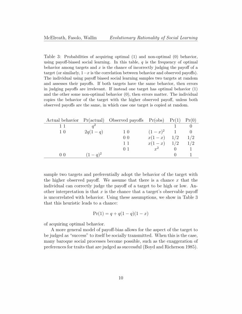
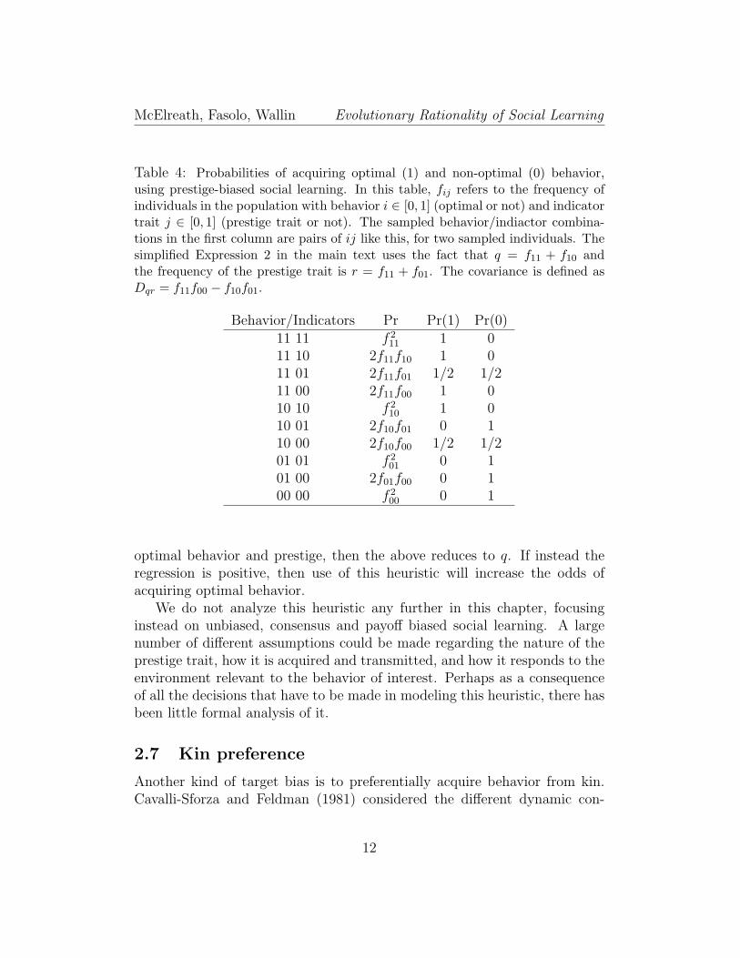
In Table 4, we derive the chance a prestige biased heuristic acquires opti-mal behavior. Let f11 be the proportion of targets with optimal behavior andthe prestige marker. Let f01 be the proportion of targets without optimalbehavior, but with the prestige marker. Then using the entries in Table 4:
Pr(1) = q +Dqr = q + var(r)βqr = q + r(1− r)βqr, (2)
where βqr = Dqr/ var(r) is the slope of the regression of optimal behavioron the prestige marker trait r. If there is no statistical associate between
11
McElreath, Fasolo, Wallin Evolutionary Rationality of Social Learning
Table 4: Probabilities of acquiring optimal (1) and non-optimal (0) behavior,using prestige-biased social learning. In this table, fij refers to the frequency ofindividuals in the population with behavior i ∈ [0, 1] (optimal or not) and indicatortrait j ∈ [0, 1] (prestige trait or not). The sampled behavior/indiactor combina-tions in the first column are pairs of ij like this, for two sampled individuals. Thesimplified Expression 2 in the main text uses the fact that q = f11 + f10 andthe frequency of the prestige trait is r = f11 + f01. The covariance is defined asDqr = f11f00 − f10f01.
Behavior/Indicators Pr Pr(1) Pr(0)11 11 f 2
11 1 011 10 2f11f10 1 011 01 2f11f01 1/2 1/211 00 2f11f00 1 010 10 f 2
10 1 010 01 2f10f01 0 110 00 2f10f00 1/2 1/201 01 f 2
01 0 101 00 2f01f00 0 100 00 f 2
00 0 1
optimal behavior and prestige, then the above reduces to q. If instead theregression is positive, then use of this heuristic will increase the odds ofacquiring optimal behavior.
We do not analyze this heuristic any further in this chapter, focusinginstead on unbiased, consensus and payoff biased social learning. A largenumber of different assumptions could be made regarding the nature of theprestige trait, how it is acquired and transmitted, and how it responds to theenvironment relevant to the behavior of interest. Perhaps as a consequenceof all the decisions that have to be made in modeling this heuristic, there hasbeen little formal analysis of it.
2.7 Kin preference
Another kind of target bias is to preferentially acquire behavior from kin.Cavalli-Sforza and Feldman (1981) considered the different dynamic con-
12

McElreath, Fasolo, Wallin Evolutionary Rationality of Social Learning
sequences of kin-biased and unbiased social learning. Boyd and Richer-son (1985) constructed several models in which parents can have differentweights in social transmission. McElreath and Strimling (2008) analyzedthe environments in which a preference for learning from parents (“vertical”transmission) is more successful than a preference for non-parents (“oblique”transmission).
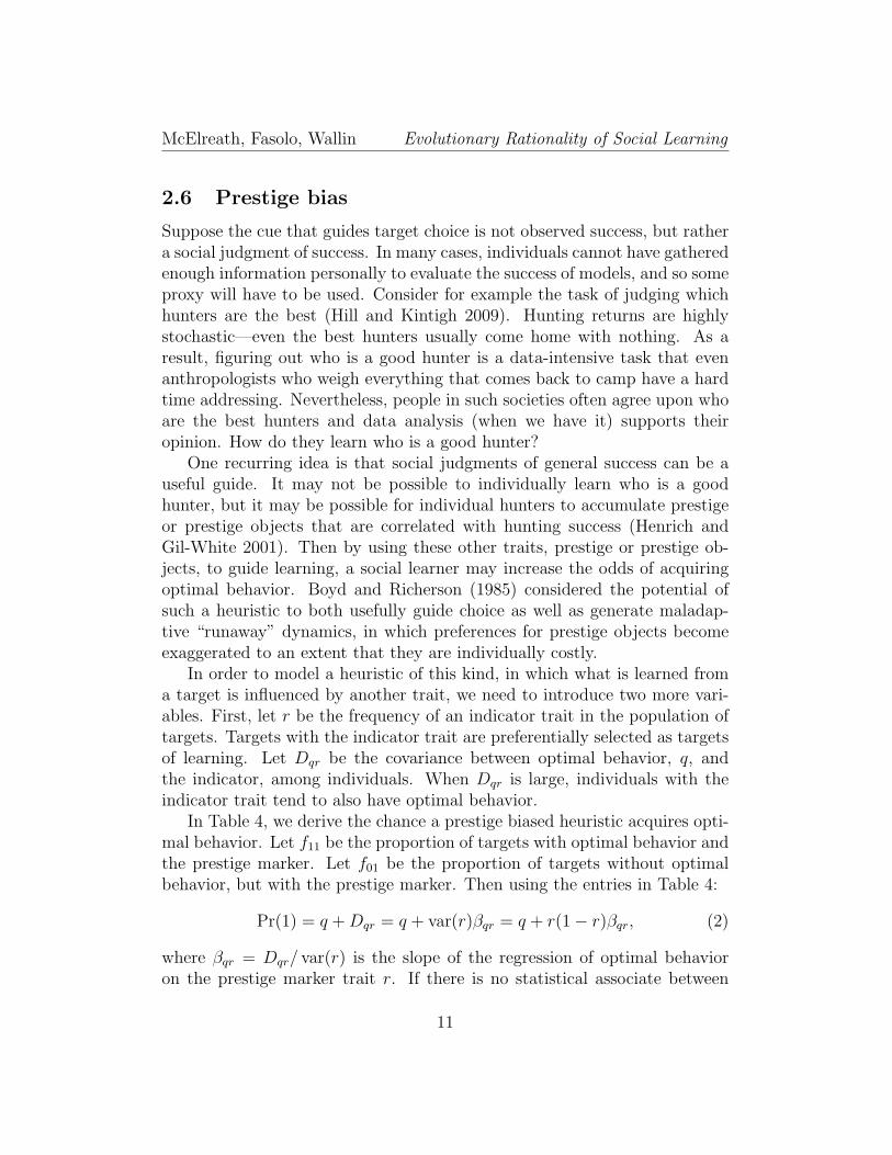
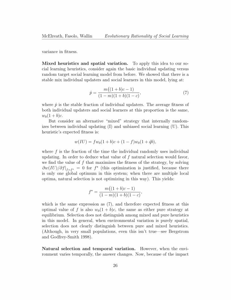
The mathematics of a kin bias heuristic are complicated. Family struc-ture has to be tracked and subtle correlations between learned behavior andlearning strategy can have powerful long-term effects. For that reason, we donot present further analysis of these heuristics in this chapter. Existing worksuggests that a kin bias will not be favored unless the relevant environmentis sufficiently unchanging and learned behavior affects fertility, rather thansurvival (McElreath and Strimling 2008). In explaining this result, it is worthnoting that a strong kin social learning preference can be favored because ofa subtle heuristic arising from the dynamics of biological reproduction andthe correlations between parents and offspring generated by heritability. If aparent having optimal behavior means that the individual has more surviv-ing children—i.e. selection affects fertility—then from a child’s perspective,the fact that her or she exists is evidence that one of his or her parents didsomething right (Figure 1). This heuristic can be quite powerful, providedoptimal behavior does not change too often so as to render past optimal be-havior non-optimal (see later section on temporal variation). But because thevalue of this parent-copying heuristic depends upon optimal behavior by aparent increasing family size, when behavior instead affects a child’s chancesof surviving to adulthood after social learning, then copying parents is neverfavored by selection, unless vertical transmission is somehow less costly ormore accurate than oblique transmission.
We note that no one has yet studied the non-linear social learning heuris-tics, like consensus and payoff bias, in combination with kin preferences.Because consensus and payoff bias depend upon sampling multiple targets,their advantages (as analyzed later in this chapter) may be limited whenrestricting sampling to kin, unless the number of close kin is quite large.Indeed, one of the wonderful complications of cultural transmission is thateach of us can have a very large number of cultural “parents,” while each ofus will always have only two genetic parents. These two facts may come intoconflict, once we consider the interaction of kin and other target based sociallearning heuristics.
13

McElreath, Fasolo, Wallin Evolutionary Rationality of Social Learning
(1)+ +
(1/2)+ +
(0) = (4 + 3/2)/9 = 0.611+ +
+
+
Vertical social learning:
Oblique social learning:
(1/4)+ +
(2/4)+ +
(3/4) = 4/9 = 0.444+ +
+
+
= = =
Figure 1: Why learning from parents, vertical social learning, can be a good sourceof adaptive behavior, compared to learning from non-parent adults, oblique sociallearning (McElreath and Strimling 2008). Family trees at the top of the figure showparents either with (gray circles) or without (black circles) optimal behavior. Eachparent with optimal behavior increases the number of surviving children born tothat family, the un-filled circles at top. Thus the family on the left, in which bothparents have optimal behavior, has four children, while the family on the right, inwhich both parents have non-optimal behavior, has only two. Below the families,we compute the chance of any child acquiring optimal behavior via either vertical(parent-child) or oblique (nonparent-child) social learning. For vertical, each childin the left family is guaranteed to get optimal behavior, while for the family on theright, none will. However, since more children in the population—across families—are born to parents with optimal behavior, if a child knows only that he or sheexists, then copying a parent can yield a higher probability of learning optimalbehavior than would copying a non-parent, which is similarly computed in thefigure. Other forces favor oblique learning, and these are discussed in McElreathand Strimling 2008.
14

McElreath, Fasolo, Wallin Evolutionary Rationality of Social Learning
Spatial Temporal
Time 1
Time 2
SpatialTemporal
+
Thursday, July 16, 2009
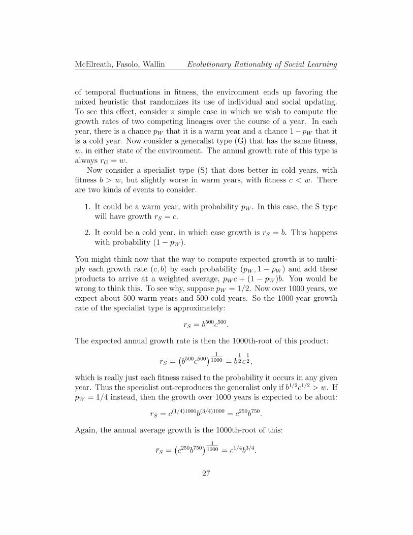
Figure 2: Abstract forms of environmental variation. Each square represents anoverhead view of environmental variation. With purely spatial variation, left col-umn, different locales favor different optimal behavior, represented by the shadinglevels. But these differences remain static through time, moving from top to bot-tom. With purely temporal variation, middle column, all locales favor the samebehavior, but the optimal behavior varies through time. With both spatial andtemporal variation, on the right, locales may be different both from other localesand from themselves, through time.
3 Ecological variation and social learning
Given the definitions of heuristics in the previous section, we now turn toanalyzing the evolutionary dynamics of these strategies, both alone and incompetition. We will assume that each heuristic is a heritable strategy andstudy their population dynamics. We focus our discussion on individual up-dating, unbiased social learning, consensus social learning, and payoff biasedsocial learning. We consider how these heuristics perform in two statisticalenvironments: (1) a spatially variable environment, in which different behav-ior is optimal in different places, and (2) a temporally variable environment,in which different behavior is optimal at different times. We also considerthe interaction of these two kinds of variation (Figure 2).
The reason for focusing on environmental variation, the rates at whichthe environment changes spatially and temporally, is that “learning” as it haslong been studied in evolutionary ecology has identified ecological variationas a prime selection pressure favoring both individual learning (phenotypicplasticity, as it is often called) and social learning (Levins 1968, Boyd andRicherson 1988). In a perfectly stationary environment, genetic adaptation
15
McElreath, Fasolo, Wallin Evolutionary Rationality of Social Learning
(canalization) does a fine job of adapting the organism, without any of thecognitive overhead and potential for error that arises from using informa-tion during development to alter behavior. Thus evolutionary ecologists stillconsider the nature of environmental variation to be a key factor in the evo-lution, maintenance, and design of learning (see e.g. Dunlap and Stephens2009, Lande 2009).
Our goal in this section is to describe some conditions under which eachsocial learning heuristic is well-adapted. No single heuristic can succeed inall circumstances. To some extent, all social learning heuristics depend uponsome kind of individual updating, for example. Additionally, the differencesamong social learning strategies generate different dynamics for the quality ofthe social environment. Because our analysis is explicitly evolutionary, it willturn out that good heuristics are those which can live well with themselves.Social heuristics tend to construct the social environments that they relyupon for information. Thus the precise ways in which the physical andsocial environments interact play a large role in determining the long-termevolutionary success of a heuristic.
Much of the analysis here is not original, but a review of a scattered liter-ature in evolutionary anthropology and ecology. However, our description ofthe effects of temporal variation and its comparison to the effects of spatialvariation is novel, to the best of our knowledge.
3.1 Spatial variation in the environment
In this section we consider the first of two stereotyped forms of environmentalvariation, spatial variation in optimal behavior. We assume that the envi-ronment is sub-divided into a large number of distinct patches, each with aunique optimal behavior. Optimal behavior within each patch is forever thesame. However neighboring patches never have the same optimal behavior.Within each patch, a large sub-population of organisms follows the life-cycle:(1) birth, (2) learning, (3) behavior, (4) migration, (5) reproduction, (6)death. Individuals are born naive and must use some strategy to acquirebehavior. If behavior is optimal for the local patch, then the individual’sfitness is multiplied by the factor 1 + b > 1. Otherwise, fitness is unchanged.A proportion m of the local population emigrates to other patches and anequally sized group immigrates from other patches. Generations overlap onlylong enough for newly born naive individuals to possibly learn from the pre-vious generation of adults. Because of migration, some of the adults available
16
McElreath, Fasolo, Wallin Evolutionary Rationality of Social Learning
to learn from are immigrants, all of whom possess non-optimal behavior fortheir new patch. While fitness is assigned in natal patches, we assume thatadults continue to display their behavior after migration, and so naive indi-viduals run the risk of learning from immigrants. Additionally, we assumethat naive individuals cannot tell who is and is not a native of their localpatch. While such cues might be available in many circumstances, they arecertainly not always available.
3.1.1 Individual updating
An individual updater (I) pays a cost c to learn the currently optimal behav-ior. The expected fitness of an individual updater is:
w(I) = w0(1 + b)c.
Provided that (1 + b)c > 1, individual updating will be the best-adaptedheuristic, whenever the quality of social information in the local patch, q, isequal to zero. However, since individual updating quickly increases the fre-quency of optimal behavior in the local patch, this heuristic quickly generatesa social environment favorable to one social learning heuristic or another.
3.1.2 Unbiased social learning
Precis. While individual updaters generate locally adaptive behavior thatsocial learners can exploit, mixing among patches erodes this information.Therefore, unbiased social learning can invade a population using individualupdating, provided mixing among patches is not too strong. Unbiased sociallearning can never completely replace individual updating, however. Thuswhen unbiased social learning can invade, there will exist a stable mix ofindividual updating and unbiased social learning in the population.
We now consider when unbiased social learning (U) can out-perform indi-vidual updating. In generation t, the expected fitness of an individual usingunbiased social learning is:
w(U)t = w0(1 + qtb),
where qt is the frequency of optimal behavior among targets in the currentgeneration t. To compute the expected fitness across generations, we need to
17

McElreath, Fasolo, Wallin Evolutionary Rationality of Social Learning
study the dynamics of q. The frequency of optimal behavior among targetsat time t is defined by the recursion:
qt = (1−m)(pt−1 + (1− pt−1)qt−1
)+m(0),
where pt−1 is the proportion of the local population comprising individualupdaters, in the previous generation. To understand this recursion, first con-sider that a proportion pt−1 of targets are individual updaters. If a sociallearning targets one of these, then it is certain to acquire optimal behavior(before migration). If instead a social learner targets another social learner,which happens 1− pt−1 of the time, there is a chance qt−1 of acquiring opti-mal behavior, because that is the chance each social learner in the previousgeneration had of acquiring optimal behavior. Finally, only a proportion1 −m of the local group remains to be potentially targets of learning. Theproportion m that immigrates possesses only non-optimal behavior, howeverit was learned.
If we assume that natural selection of the frequencies of learning heuristicsis slow relative to the dynamics of q, then we can treat pt as a constant pin the expression above and set qt = qt−1 = q and solve for the expectedproportion of optimal behavior among targets:
q =(1−m)p
1− (1−m)(1− p). (3)
Numerical works shows that this fast-slow dynamics approximation is veryaccurate, unless selection (proportional to b) is very strong. Because changesin the frequency of locally optimal behavior occur much faster than changesin the frequencies of learning heuristics, the expression above allows us tocompute the proportion of optimal behavior that selection will act on, forany value of p.
The expression for q tell us some interesting things right away. If there isno migration, all behavior eventually becomes optimal, q|m=0 = 1. If thereare no individual updaters (p = 0), then eventually no behavior is optimal,q|p=0 = 0.
Using the expression q and the fitness expressions for individual updating(I) and unbiased social learning (U), we can derive the conditions for eitherheuristic to exclude the other. As has been shown many times (see Rogers1988 for a clear example), neither individual updating nor unbiased sociallearning can exclude one another under all circumstances, and so models ofthis kind predict that both will co-exist, in the absence of other heuristics.
18
McElreath, Fasolo, Wallin Evolutionary Rationality of Social Learning
First, consider when individual updating can resist invasion by rare sociallearners. This requires:
w(I) > w(U)|p=1,
m > (1 + b)(1− c)/b.
If migration is too common, then unbiased social learning cannot invade apopulation of individual updaters, because too often the behavior availableto copy is appropriate for only a neighboring patch. However the amount ofmigration unbiased social learning can tolerate depends upon the costs andbenefits of learning. As b increases, the above condition is easier to satisfy.At the limit b→∞, the condition approaches m > 1− c, and so as long asmigration is lower than the fitness lost via individual updating, individualupdating can never exclude unbiased social learning.
When unbiased social learning is able to invade, it will completely replaceindividual updating if:
w(U)|p=0 > w(I),
(1 + b)c < 1.
As long as individual updating is worth using at all, unbiased social learningcan never completely replace it.
These two results imply that when m < (1 + b)(1− c)/b, a stable mix ofindividual updating and unbiased social learning should exist in the popula-tion. The stable proportion of individual updaters, p, is found where:
w(I) = w(U)|p=p,
p =m((1 + b)c− 1
)(1−m)(1 + b)(1− c)
. (4)
Inspecting the partial derivatives of the right-hand side shows that ∂p/∂m >0, ∂p/∂b > 0, and ∂p/∂c > 0, for all b > 0, c ∈ [0, 1],m ∈ [0, 1], (1 + b)c > 1.Therefore increasing migration, increasing the value of optimal behavior,and decreasing the cost of individual updating all increase the equilibriumfrequency of individual updating.
3.1.3 Consensus social learning
Precis. Consensus social learning yields higher fitness and replaces unbi-ased social learning, provided mixing between patches is not so strong as to
19
McElreath, Fasolo, Wallin Evolutionary Rationality of Social Learning
make the expected local proportion of optimal behavior below one-half. Ifmixing is sufficiently weak and individual updating sufficiently costly, thenconsensus social learning can actually out-compete both individual updatingand unbiased social learning.
When can a consensus learning heuristic invade a population of individualupdaters and social learners? We derived above that, when the environmentvaries spatially, the population will approach a stationary proportion of in-dividual updaters, unless migration is very powerful relative to the value ofoptimal behavior, in which case individual updating will dominate. At thestationary mix of both heuristics, the expected fitness of both individual up-dating and unbiased social learning is w0(1 + b)c. For consensus learning toinvade, it only has to achieve greater fitness than this.
The expected fitness of a rare consensus learner (C) in generation t is:
w(C)t = w0(1 + b(qt + qt(1− qt)(2qt − 1)),
where the factor qt + qt(1− qt)(2qt − 1) was derived in Table 2. The invaderfaces a value of qt = q, reached under the joint action of both individualupdaters and unbiased social learners. But regardless of the value of q, forconsensus learning to do better than either common heuristic, all that isrequired is that:
w(C)t > w0(1 + qtb) =⇒ qt >1
2.
Consensus social learning is favored in any generation in which the expectedproportion of optimal behavior among targets is greater than one-half. Sub-stituting in the expression for q, this condition simplifies to:
m <p
1 + p.
So as long as migration isn’t so strong as to flood local adaptive learning,which happens at a rate p, consensus learning can invade a mix of individualupdating and social learning. Since p is a function of m, b, c, we can substitutein the expression for p derived in the previous section. The condition m <p/(1 + p) is satisfied when:
b >1− cc− 1
2
.
20

McElreath, Fasolo, Wallin Evolutionary Rationality of Social Learning
The right-hand side decreases as c increases, making the condition easierto satisfy (for c > 1/2). This means that consensus learning can invade,provided that individual updating is sufficiently cheap (remember: high cmeans cheap updating). If c is too small (too costly), then there won’t beenough individual updating at equilibrium to keep the average q above one-half. That is, consensus learning can invade only if conditions favor individualupdating enough to ensure that the average qt > 1/2.
Now, can consensus learning ever exclude simple social learning? In orderfor consensus learning to exclude simple social learning, it is still necessarythat q > 1/2. But as consensus learning increases in frequency, it will ex-aggerate any initial qt > 1/2, because consensus learning increases q fromgeneration to generation (assuming q > 1/2), as compared to simple so-cial learning, which just replicates q from generation to generation. Thismeans that the advantage consensus learning has over simple social learningwill only increase as consensus increases in frequency. Therefore consensuslearning will exclude and replace simple social learning in this environment,whenever it can invade.
Perhaps counter-intuitively, if the rate of mixing is low enough, consensuslearning can exclude even individual updating, which simple social learningcan never do. If consensus learning is common, then the expected proportionof locally optimal behavior is:
q = (1−m)(q + q(1− q)(2q − 1)
)=
3(1−m) +√
(1−m)(1− 9m)
4(1−m).
This expression is hard to interpret directly, but for small m (such thatm2 ≈ 0, it is approximately 1−m, which shows that migration tends to reducethe proportion of locally optimal behavior as you might expect. Using theexact expression, consensus learning can exclude individual updating whenw0(1 + bq) > w0(1 + b)c, which is satisfied when both m ≤ 1/9 and c ≤ 3/4.Provided migration is weak and individual updating is sufficiently expensive,consensus learning can dominate.
The exact result here depends critically on the precise model of consensuslearning. However, the qualitative result is likely quite general. Consensuslearning is a non-linear form of cultural updating. As a consequence, itcan actively transform the frequency of behavior from one generation to thenext. It is a form of “inference,” to speak casually. When mixing is weak,this inferential process can substitute for costly individual updating, because
21
McElreath, Fasolo, Wallin Evolutionary Rationality of Social Learning
the increase in locally optimal behavior consensus learning generates eachgeneration will balance the loss from immigration.
However, as we will show when we explore temporal variation, this resultis quite fragile. It depends upon the environment’s being stable through time(Whitehead and Richerson 2009).
3.1.4 Payoff bias
Precis. Payoff biased social learning can, like consensus social learning,replace both unbiased social learning and individual updating, under the rightconditions. If migration is weak enough and error in judging payoffs greatenough, then consensus social learning can out-compete payoff biased learn-ing.
Payoff biased social learning relies upon the observable consequences ofprevious choice. As a result, the lower the correlation between observablesuccess and optimal behavior in the relevant domain, the lower the benefitpayoff biased learning provides.
Payoff bias can always invade and replace unbiased social learning. Thecondition for payoff bias to invade a population of individual updaters andunbiased social learners is:
w0(1 + b(qt + qt(1− qt)(1− x))) > w0(1 + bqt),
The above simplifies to x < 1 for all qt ∈ [0, 1], and so payoff biased learningdominates unbiased social learning whenever there is any correlation betweenobservable success and the behavior of interest.
Like consensus learning, payoff bias is non-linear and actively changes thefrequency of adaptive behavior from one generation to the next. Also likeconsensus learning, this means payoff bias can sometimes exclude individ-ual updating. The stable value of q, in a population with only payoff biaslearning, is:
q = (1−m)(q + q(1− q)(1− x)
)= 1− m
(1−m)(1− x). (5)
The effect of both x and m is to reduce q. More migration means more im-migrants with non-optimal behavior. Higher x means more errors in judgingpayoffs, which means more (effectively) unbiased social learning. When xand m are both small, however, q can be nearly 1.
22

McElreath, Fasolo, Wallin Evolutionary Rationality of Social Learning
Using this expression for q, payoff bias learning can exclude individualupdating, provided:
w0(1 + b)c < w0(1 + b(q + q(1− q)(1− x))),
x < 1− m
1−m· b
b− (1−m)((1 + b)c− 1). (6)
This expression is hard to interpret, but again, if we assume m is small sothat m2 ≈ 0, then it simplifies to x < 1−mb/((1 + b)(1− c)). So as long asmigration is not too strong and individual updating is sufficiently costly, itis possible for payoff bias to completely exclude individual updating.
Finally, consensus social learning can sometimes invade and replace payoffbiased social learning. Analyzing the case of consensus invading a stablemix of individual updating and payoff bias is difficult and results in messyexpressions that hard to interpret. However the case of consensus invadinga population of pure payoff bias (condition 6 satisfied) is easier and revealsmany of the same intuitions. Consensus can invade a pure population ofpayoff biased social learning and replace it, provided:
w(P )|q=q <w(C)|q=q,
m <x(1− x)
x(1− x) + 2.
This condition can also be derived by noting that consensus out-performspayoff bias when:
2q − 1 > 1− x =⇒ q > 1− x/2.
Substituting in the value of q when payoff bias is common, Expression 5, thissimplifies to the same condition as above.
When x is very small, payoff biased learning is highly accurate and there-fore unless migration is also very weak, consensus learning lacks a sufficientadvantage.
3.1.5 Summary
All of the above results explore the properties of unbiased, consensus, andpayoff bias social learning when the environment varies spatially. We showedthat unbiased social learning can never completely replace individual updat-ing of some kind, because unbiased learning does not transform the frequency
23
McElreath, Fasolo, Wallin Evolutionary Rationality of Social Learning
of optimal behavior. As a result, it does nothing to modify its social envi-ronment for its own good. In contrast, both consensus bias and payoff biasactively transform the frequency of optimal behavior across generations, in-creasing it slightly above its previous value (assuming q > 1/2, x < 1). Asa result, both consensus and payoff bias can completely exclude individualupdating, provided the force of mixing, m, isn’t too strong and individualupdating is sufficiently costly.
We think such conditions are actually quite rare (and as we show in thenext sections, completely absent under our model of temporal environmentalvariation), but they do reveal a fundamental property of these non-linearsocial learning heuristics: they actively modify their social environment, andthis process can substitute for individual updating, in the right kinds of envi-ronments. But each heuristic modifies the social environment using differentcues, and therefore they behave differently in different environments. As weshow in the next section, consensus and payoff bias behave quite differentlywhen the environment varies in time, rather than in space.
We also found that either consensus or payoff bias can dominate the other,depending upon the amount of mixing among patches (m) and the amountof error in judging payoffs (x).
3.2 Temporal variation
When the environment varies through time, instead of across space, many ofthe same principles that we discovered above hold true. However, there areimportant differences between temporal variation and spatial variation. Un-der purely spatial variation in optimal behavior, individuals do well to avoidlearning from immigrants to their local patch. However, since the locallyoptimal behavior does not change over time, a reliable store of locally adap-tive culture can accumulate (as long as mixing isn’t too strong). Indeed, weshowed that both consensus and payoff bias can even exclude individual up-dating, maintaining optimal behavior at high frequency, even though neitheruses individual experience with the environment.
When the environment varies through time, the nature of the problemis subtly different. Now the optimal behavior in each patch will eventu-ally change. When it does, all previously learned behavior is rendered non-optimal. As a result, all social learning heuristics are at a disadvantage, justafter a change in the environment. Specifically, we will assume that the en-vironment no longer varies spatially—all patches favor the same behavior.
24
McElreath, Fasolo, Wallin Evolutionary Rationality of Social Learning
However, there is a chance u in each generation that all patches switch tofavoring a new behavior. Since there is a very large number of alternativebehaviors, all previously learned behavior is then non-optimal.
This kind of environmental variation also forces us to contend with whatevolutionary ecologists call geometric mean fitness (see Orr 2009 for a recentreview and comparison of different evolutionary concepts of fitness). Whenenvironments vary through time, even rare catastrophe can mean the endof a lineage. As a result, selection may favor risk-averse strategies that areadapted to statistical environments, instead of current environments (Gille-spie 1974, Levins 1968).
3.2.1 Temporal variation may favor randomized or mixed strate-gies
Precis. A mixed heuristic is one in which individuals use two or moreheuristics different proportions of the time. When the environment variespurely across space, selection does not clearly favor either pure social learningheuristics or mixed social learning heuristics. When the environment variesthrough time, however, selection favors mixed heuristics over pure ones. Inthe case of of unbiased social learning and individual updating, selection fa-vors the mixed heuristic of these two over both pure strategies. At evolution-ary equilibrium, the proportion of time individuals using the mixed heuristicdeploy individual updating may be either more or less than the stable propor-tion of pure individual updating favored under pure spatial variation in theenvironment.
One important result of temporal variation is that a strategy that mixes in-dividual updating and social learning will often out-compete both pure strate-gies. In the spatial variation case, it makes no obvious difference whetherindividuals randomly update for themselves or learn socially. But when theenvironment varies through time, natural selection will tend to favor “bethedging” strategies that engage in adaptive randomization of behavior. Themathematics can be opaque at first, but grasping the cause is easy: survivaland reproduction are multiplicative processes. As a result, if a lineage ever isreduced to a very small number of individuals, then it will take it a long timeto recover. Therefore a strategy has to both do well and avoid bottlenecks inorder to grow quickly and sustain its numbers. When selection varies tem-porally, selection favors heuristics that attend both mean fitness as well as
25
McElreath, Fasolo, Wallin Evolutionary Rationality of Social Learning
variance in fitness.
Mixed heuristics and spatial variation. To apply this idea to our so-cial learning heuristics, consider again the basic individual updating versusrandom target social learning model from before. We showed that there is astable mix individual updaters and social learners in this model, lying at:
p =m((1 + b)c− 1)
(1−m)(1 + b)(1− c), (7)
where p is the stable fraction of individual updaters. The average fitness ofboth individual updaters and social learners at this proportion is the same,w0(1 + b)c.
But consider an alternative “mixed” strategy that internally random-izes between individual updating (I) and unbiased social learning (U). Thisheuristic’s expected fitness is:
w(IU) = fw0(1 + b)c+ (1− f)w0(1 + qb),
where f is the fraction of the time the individual randomly uses individualupdating. In order to deduce what value of f natural selection would favor,we find the value of f that maximizes the fitness of the strategy, by solving∂w(IU)/∂f |f=f? = 0 for f ? (this optimization is justified, because thereis only one global optimum in this system; when there are multiple localoptima, natural selection is not optimizing in this way). This yields:
f ? =m((1 + b)c− 1)
(1−m)(1 + b)(1− c),
which is the same expression as (7), and therefore expected fitness at thisoptimal value of f is also w0(1 + b)c, the same as either pure strategy atequilibrium. Selection does not distinguish among mixed and pure heuristicsin this model. In general, when environmental variation is purely spatial,selection does not clearly distinguish between pure and mixed heuristics.(Although, in very small populations, even this isn’t true—see Bergstromand Godfrey-Smith 1998).
Natural selection and temporal variation. However, when the envi-ronment varies temporally, the answer changes. Now, because of the impact
26
McElreath, Fasolo, Wallin Evolutionary Rationality of Social Learning
of temporal fluctuations in fitness, the environment ends up favoring themixed heuristic that randomizes its use of individual and social updating.To see this effect, consider a simple case in which we wish to compute thegrowth rates of two competing lineages over the course of a year. In eachyear, there is a chance pW that it is a warm year and a chance 1− pW that itis a cold year. Now consider a generalist type (G) that has the same fitness,w, in either state of the environment. The annual growth rate of this type isalways rG = w.
Now consider a specialist type (S) that does better in cold years, withfitness b > w, but slightly worse in warm years, with fitness c < w. Thereare two kinds of events to consider.
1. It could be a warm year, with probability pW . In this case, the S typewill have growth rS = c.
2. It could be a cold year, in which case growth is rS = b. This happenswith probability (1− pW ).
You might think now that the way to compute expected growth is to multi-ply each growth rate (c, b) by each probability (pW , 1 − pW ) and add theseproducts to arrive at a weighted average, pW c + (1 − pW )b. You would bewrong to think this. To see why, suppose pW = 1/2. Now over 1000 years, weexpect about 500 warm years and 500 cold years. So the 1000-year growthrate of the specialist type is approximately:
rS = b500c500.
The expected annual growth rate is then the 1000th-root of this product:
rS =(b500c500
) 11000 = b
12 c
12 ,
which is really just each fitness raised to the probability it occurs in any givenyear. Thus the specialist out-reproduces the generalist only if b1/2c1/2 > w. IfpW = 1/4 instead, then the growth over 1000 years is expected to be about:
rS = c(1/4)1000b(3/4)1000 = c250b750.
Again, the annual average growth is the 1000th-root of this:
rS =(c250b750
) 11000 = c1/4b3/4.
27

McElreath, Fasolo, Wallin Evolutionary Rationality of Social Learning
In general, if the environment varies temporally between two states, eachwith probability p1 and p2 respectively, then the long-term growth rate is:
r = wp1
1 wp2
2 .
This is in fact the geometric mean fitness of the strategy. Natural selec-tion in temporally varying environments will tend to (locally) maximizegeometric mean fitness, not arithmetic mean fitness. Evolutionary ecol-ogists usually work with the natural logarithm of this average, log[r] =p1 log[w1] + p2 log[w2], because it tends to make the maths easier. Any strat-egy that maximizes r will also maximize log[r], and so the transformation isharmless.
In the case of analyzing social learning, the state of environment is thetime since the environment last changed, and this could be anything from onegeneration ago to an infinity of generations ago. This might seem dauntingat first, but it is really just an application of the logic above, extrapolatingfrom two states of the environment to an infinity of states. The kind of fitnessexpression we seek is log[r] =
∑ni=1 pi log[wi], for n environmental states and∑n
i=1 pi = 1. We use this definition of fitness in the next section, to showhow temporal variation favors mixed social learning heuristics.
Temporal variation and social learning. We will assume again thatthere are a large number of alternative behaviors, but instead of pure spatialvariation, we will now assume that there is purely temporal variation. Eachgeneration, there is a chance u that the environment changes and makesanother random behavior optimal, rendering all previously learned behaviornon-optimal. Let p again be the frequency of individual updating in the pop-ulation. One generation after a change in the environment, the proportion ofadaptive behavior is q(1) = p, because individual updaters have had one gen-eration to pump new knowledge into the society. After one more generationwithout another change, q(2) = p+ (1− p)q(1) = p+ (1− p)p = 1− (1− p)2.Then q(3) = p+ (1− p)q(2) = 1− (1− p)3. This series continues and impliesthat, if the environment changed t > 0 generations ago, the expected chanceof acquiring optimal behavior via social learning is:
q(t) =t∑
i=1
p(1− p)i−1 = 1− (1− p)t. (8)
In Figure 3, we plot this function against time for two values of p.
28
McElreath, Fasolo, Wallin Evolutionary Rationality of Social Learning
0 5 10 15 20 25 30
0.00.20.40.60.81.0
time since last change in environment
q(t)
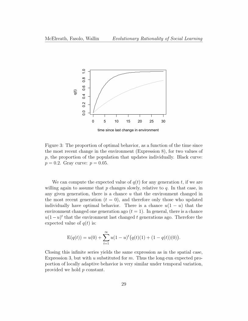
Figure 3: The proportion of optimal behavior, as a function of the time sincethe most recent change in the environment (Expression 8), for two values ofp, the proportion of the population that updates individually. Black curve:p = 0.2. Gray curve: p = 0.05.
We can compute the expected value of q(t) for any generation t, if we arewilling again to assume that p changes slowly, relative to q. In that case, inany given generation, there is a chance u that the environment changed inthe most recent generation (t = 0), and therefore only those who updatedindividually have optimal behavior. There is a chance u(1 − u) that theenvironment changed one generation ago (t = 1). In general, there is a chanceu(1−u)t that the environment last changed t generations ago. Therefore theexpected value of q(t) is:
E(q(t)) = u(0) +∞∑
t=1
u(1− u)t(q(t)(1) + (1− q(t))(0)
).
Closing this infinite series yields the same expression as in the spatial case,Expression 3, but with u substituted for m. Thus the long-run expected pro-portion of locally adaptive behavior is very similar under temporal variation,provided we hold p constant.
29
McElreath, Fasolo, Wallin Evolutionary Rationality of Social Learning
But p will not be constant under natural selection, and in the temporalcase, the effect of q(t) on fitness will be quite different. Instead of using theabove expectation directly to compute fitness, we must use it to build thelong-run growth rate of the social learning heuristic. Using the definition oflog geometric mean fitness, we build the growth rate of an unbiased sociallearner (U) by multiplying each probability of each environmental state bythe log-fitness in that state.
r(U) = u log[w0] +∞∑
t=1
u(1− u)t log[w0(1 + bq(t))].
The above can be motivated in the following way. Expected fitness is theproduct of each fitness raised to the probability of its occurrence, so theexpected log-fitness is the sum of each log-fitness multiplied by the probabilityit occurs. If the environment has just changed, which happens u of the time,then the individual receives w0. The other possibility is that the environmenthas not changed in the last t generations, yielding a chance q(t) of fitnessw0(1 + b) and a chance 1 − q(t) of fitness w0, for each individual using thisheuristic. That is, every social learner experiences the same q(t) in anygeneration t, and the value of q(t) is determined by the probabilities u(1−u)t.But a proportion q(t) of social learners will get lucky and choose a targetwith optimal behavior, while the rest will not. Thus the probability q(t) isinside the logarithm.
Unfortunately, placing q(t) inside the logarithm makes the mathematicsintractable. There are no algebraic methods for closing such an infinite sum,in which the power t is both outside and inside the logarithm. We can makeprogress, however, by constructing an approximation that is valid for weakselection, when b, c are small such that terms of order b2 and (1 − c)2 andgreater are approximately zero. The use of weak selection approximations iscommon in evolutionary ecology, because it often makes otherwise intractableproblems analytically solvable. One must keep in mind, however, that ourconclusions from here out will only be exactly valid for choices that havemodest effects on fitness. Numerical work, as well as the simulations weshow in a later section, confirm that the qualitative conclusions we reachhere are general to strong selection, however.
To apply the weak selection approximation, we use a Taylor series expan-sion of r(U) around b = 0, c = 1 and keep the linear terms in b, c. This gives
30

McElreath, Fasolo, Wallin Evolutionary Rationality of Social Learning
us:
r(U) ≈ log[w0] +(1− u)bp
1− (1− p)(1− u).
We wish to compare this expression to the weak-selection approximationof the growth rate of individual updating, which by the same method isr(I) ≈ log[w0] + b− (1− c). Selection will adjust p until r(U) = r(I), whichimplies an expected long-run value of p:
p =u(b− (1− c))(1− u)(1− c)
. (9)
This is the same as Expression 7, once we apply the weak selection approxi-mation and let m = u. We will need this result in order to compare the twopure heuristics to the mixed heuristic in the temporal variation context.
Temporal variation favors mixed heuristics. Now again consider thefamily of alternative heuristics that randomize their updating, using individ-ual updating (I) a proportion f of the time and unbiased social updating (U)a proportion 1− f of the time. Using the same logic that allows writing theexpression r(U) above, the long-run growth of this mixed heuristic is:
r(IU) =∞∑
t=0
u(1− u)t log[fw0(1 + b)c+ (1− f)w0(1 + bq(t))].
Assuming the IU heuristic is rare and that q(t) is therefore determined onlyby the proportions of pure individual and social updaters, p, and again thatselection is weak, the above closes to:
r(IU) ≈b(p(1− u) + uf(1− (1− c)(1− f))
)1− (1− p)(1− u)
+ (1− c)f + log[w0].
By comparing the above to the growth rates for the pure strategies, itturns out that this mixed strategy can invade the stable mix of pure strate-gies, for any value of f . The condition for a rare IU individual to invadethe mix of I and U is r(IU)|p=p > r(I), where p is defined by Expression 9.This condition is satisfied for all b > 0, 0 < c < 1, 0 < u < 1, which meansthe mixed strategy can always invade a population of pure heuristics. Thiskind of result is typical of game theoretic solutions of this kind. The value
31
McElreath, Fasolo, Wallin Evolutionary Rationality of Social Learning
of f does not matter for invasion, because whatever the value of f , the firstmixed strategy individual will behaviorally simulate either a pure I or a pureU individual. Since both I and U have the same fitness at p = p, it makesno difference which of these heuristics is realized.
The value of f will matter, however, as IU increases in frequency. Oncecommon, it turns out that the mixed heuristic IU is also always stable againstinvasion by pure I and U. To prove this we need to calculate the optimal valueof f = f ? that no other value of f can invade. When IU is common, theproportion of optimal behavior is now given by:
q(t) =t∑
i=1
f ?(1− f ?)i−1,
where f ? is the common chance a IU individual updates individually. Theevolutionarily stable value of f ? is found where:
∂r(IU)
∂f
∣∣∣∣f=f?
= 0.
Again using a weak selection approximation and solving the above for f ?
yields:
f ? =u((1 + b)c− 1 + u((1− b)(1− c)− b)
)(1− c)(1− u)2
. (10)
By substituting the value of f ? back into r(IU), one can derive the growthrate of the mixed strategy when it is common and using the optimal valueof f . We ask when:
r(IU)|f=p=f? > r(I),
r(IU)|f=p=f? > r(U)|p=f? .
Both of these conditions are true for all b > 0, 0 < c < 1, 0 < u < 1, and sothe mixed heuristic can both invade a population of pure heuristics as wellas resist invasion by either pure heuristic.
The mixed heuristic that randomly uses individual and social updatingboth invades and replaces a population of pure individual and social up-daters. This was not the case for purely spatial environmental variation.The reason for the different result owes to bet-hedging (Philippi and Seger
32

McElreath, Fasolo, Wallin Evolutionary Rationality of Social Learning
1989) against the small payoff to social updaters, soon after a change inthe environment. Because the mixed heuristic spreads its bets over twodifferent portfolio options—individual updating and social updating—it ex-periences reduced risk of ruin, like pure individual updating, but also reapshigher rewards when the quality of socially learned behavior is high, likeunbiased social learning. This is mathematically homologous to human in-vestors spreading risk over multiple stocks, because even if the chance of anyindividual stock losing most of its value is low, if all assets are placed in a sin-gle stock, eventually all of one’s assets will lose most of their value. Similarly,the mixed heuristic out-performs both pure heuristics, because this strategyis never entirely ruined by a change in the environment, but neither does itentirely forgo the gains to social learning that accrue when the environmentremains stable. Both pure heuristics instead take risks by betting entirely onone kind of event or the other.
Because there are two kinds of risks, it is not true that the mixed strategyalways individually updates more than the population of pure strategies.Instead, depending upon how uncertain the environment is, the mixed IUheuristic adjusts the amount of probability in individual updating. Whenthe environment is rather stable, IU tends to individually update less thanthe population of pure types. It is possible to derive a threshold value of ubelow which IU uses individual updating less than p (9) and above which IUuses individual updating more than p. However, this expression is a complexfunction of b, c and provides little by way of intuition.
The important lesson here is that temporal variation strongly favors afundamentally different way of combining heuristics, mixing them withinindividuals rather than among individuals. In this way, the physical environ-ment, whether variation is spatial or temporal, favors different social learningstrategies and combinations of those strategies. This in turn leads us to makedifferent predictions about the kinds of heuristics that will be adapted to dif-ferent domains of behavior, depending in part upon the relative strengths ofspatial and temporal variation.
It should be noted, however, that the model in this section is still just amodel—it is limited to fairly particular assumptions about the environmentand the heuristics. The temporal variation here is not auto-correlated—ifthe environment has just changed, it no more or less likely to change again.Real environments, ecological measurements suggest, tend to include a goodamount of autocorrelation, as evidenced by “red” noise in their time series(Whitehead and Richerson 2009). While we see no reason that the conclu-
33
McElreath, Fasolo, Wallin Evolutionary Rationality of Social Learning
sions here should not extend, qualitatively, to autocorrelated environments,we do believe that it is a problem worth modeling.
3.2.2 Consensus learning less favored under temporal variation
Precis. When the environment varies through time, consensus social learn-ing does much worse than it does under spatial variation. It can never excludeindividual updating, because every time the environment changes, q < 1/2 forat least one generation and consensus learners do badly compared to unbiasedlearners. However, adding in some spatial variation as well helps consensuslearning recover.
In the case of purely spatial variation, we previously demonstrated that con-sensus social learning can in fact exclude both simple social learning andindividual updating, provided the rate of mixing between locales is suffi-ciently low. Under purely temporal variation, consensus learning can neverexclude the other learning heuristics. Just after a change in the optimalbehavior, all previously-learned behavior is non-optimal. Therefore inferringbehavior from the majority will lead to stabilizing non-adaptive behavior.As a result, consensus learning depends upon some other heuristic—or mixof heuristics—to increase the frequency of newly-optimal behavior, after achange in the environment.
The mathematics of this case are complex, because accounting for geomet-ric fitness effects and the non-linearities of consensus learning is analyticallydifficult. But the results are easy to visualize in simulation from the fitnessdefinitions. Figure 4 plots the proportions of individual updating (gray), un-biased social learning (blue), and consensus learning (red) through time, forboth pure spatial and pure temporal environmental variation. In the absenceof temporal variation in optimal behavior, consensus learning can actuallyexclude both individual updating and unbiased social learning (top panel).However, under temporal variation in the environment, consensus learningdoes quite poorly, owing to its drop in frequency each time the environmentshifts from one optimal behavior to another. A mix of individual updatingand unbiased social learning evolves.
A small amount of spatial variation and mixing can go a long way to-wards helping consensus social learning, however (Figure 5). While temporalvariation hurts consensus learning much more than it hurts unbiased sociallearning, spatial variation and mixing hurts unbiased learning more than it
34

McElreath, Fasolo, Wallin Evolutionary Rationality of Social Learning
hurts consensus social learning. After a change in the environment, consensussocial learners suffer reduced fitness, declining in frequency as individual up-dating increases in frequency (see time series in Figure 5). But once the localfrequency of optimal behavior has increased, unbiased social learners have noparticular advantage over consensus social learners. Meanwhile, consensussocial learners avoid learning from immigrants with behavior adapted to otherpatches, while unbiased social learners do not. Reintroducing mixing amongspatially variable patches provides a constant environmental challenge thatpartially resuscitates consensus learning. Therefore it is not a valid conclu-sion that consensus learning is poorly adapted whenever environments varythrough time. Instead, we should conclude that temporal variation worksagainst consensus learning, while mixing and spatial variation work for it. Ifeither force is strong enough, it can eclipse the other.
We caution the reader to note that the same principle will hold in the caseof consensus social learning in temporally varying environments that holdsfor unbiased social learning: a mixed individual updating and consensusstrategy will do better than a mix of pure strategies. We do not belaborthis point here, because we know of no additional intuitions to be acquiredfrom the analysis. But we do not want readers to conclude that mixedrandomizing heuristics would not be favored for consensus learning as theywould be for unbiased social learning. Indeed, the bet-hedging will arguablybe stronger in the case of consensus learning, because the effects of a recentchange in the environment are harsher for consensus learning than they arefor unbiased social learning. At the same time, since consensus learning candrive the proportion of optimal behavior both down (when q < 1/2) as wellas upwards (when q > 1/2), the dynamics may be much more complex andinteresting.
3.2.3 Summary
In this section, we analyzed the effects of temporal environmental variationon unbiased and consensus social learning heuristics. Temporal variationrequires a different approach to calculating evolutionarily-relevant payoffs,because if a strategy is reduced to zero numbers in any generation, thenthe strategy is dead forever. This “bottleneck” effect can have importantconsequences for the evolutionary rationality of heuristics. This principlelead us to two main results.
First, temporal variation can favor internally mixed heuristics, when
35

McElreath, Fasolo, Wallin Evolutionary Rationality of Social Learning
100 200 300 400 500time
0.2
0.4
0.6
0.8
1.0
frequency
100 200 300 400 500time
0.2
0.4
0.6
0.8
frequency
Figure 4: Stochastic simulations of the evolution of consensus learning, undereither spatial or temporal environmental variation. The gray trend in eachpanel is the proportion of the population that uses individual updating. Theblue and red curves are unbiased social learning and consensus learning, re-spectively. In both panels, b = 0.5, c = 0.8. Initial proportions for individual,unbiased, and consensus: 0.8, 0.1, 0.1. Top panel: Purely spatial variation,m = 0.05. Consensus learning evolves to exclude both individual and un-biased social learning. Bottom panel: Purely temporal variation, u = 0.05.Consensus learning now does much worse, owing to its inability to increasethe frequency of novel adaptive behavior.
36

McElreath, Fasolo, Wallin Evolutionary Rationality of Social Learning
100 200 300 400 500time
0.2
0.4
0.6
0.8
frequency
Figure 5: Stochastic simulations of the evolution of consensus learning, un-der simultaneous spatial and temporal environmental variation. The graytrend is the proportion of the population that uses individual updating. Theblue and red curves are unbiased social learning and consensus learning, re-spectively. Same parameter values and initial proportions as in Figure 4.Consensus social learning can out-compete unbiased social learning, even inthe presence of temporal variation, provided there is enough mixing amongspatially variable patches. Here, u = m = 0.05.
purely spatial variation does not. The reason is that temporal variationfavors bet-hedging heuristics that spread risk across alternative behavioralstrategies. In this case, a mixed strategy that randomly deploys individualupdating and unbiased social updating always replaces a population of pureindividual updating and unbiased social learning strategies, when there ispurely temporal variation in the environment.
Second, consensus social learning is disadvantaged under temporal varia-tion. The reason is that, just after a change in the environment, all learnedbehavior is non-optimal. As a consequence, the majority behavior providesan invalid cue to optimality. Once some other heuristic or set of heuristicshave again increased optimal behavior in the population, consensus can dowell, but lost fitness during the transition can cause it to be out-competed byother learning heuristics. This does not happen under purely spatial varia-tion, because a constant stream of immigrants actually provides an environ-mental challenge that consensus learning is well-suited to, provided that mix-ing is not so strong as the make the majority of local behavior non-optimal.Simultaneously combining spatial and temporal variation shows that consen-sus learning can be profitable when temporal variation is present, provided
37
McElreath, Fasolo, Wallin Evolutionary Rationality of Social Learning
that there is enough spatial mixing and spatial variation.
4 Conclusion
We have tried to show how the way in which optimal behavior varies acrossspace or through time favors different social learning heuristics. We are skep-tical that there will be any learning strategy, social or not, that is best inall contexts. Instead the type of analysis in this chapter suggests that ei-ther over evolutionary or developmental time, individuals acquire strategiesthat exploit patterns in specific environments. In this way, the tradition inevolutionary ecology of studying cognitive adaptation via social learning isquite similar to the tradition in bounded rationality. And like some analy-ses in bounded rationality, the environments in this chapter are statistical.Instead of adapting to a single state of the world, the theoretical organismsin our thought experiments adapt to a statistical world in which random-ness and variation present survival challenges. Successful heuristics are theones that out-reproduce competitors over many generations of learning andchoice, sometimes hedging their bets against unpredictable bad times. Inany particular generation, a social learning heuristic can appear nonsensical.It is in the long run, across the full distribution of environmental dynamics,that the evolutionary rationality of each heuristic appears.
The breadth of issues relevant to the evolution of social learning is huge.We have focused on the nature of environmental variation, because this topichas long been central to the study of learning, social or not, in evolutionaryecology (Levins 1968). Indeed, fluctuating selection has turned out to becentral to broad debates that touch upon most corners of evolutionary biology(Gillespie 1994). Organisms are not adapted to a static world of stationarychallenges, but rather a mosaic world that varies across space and fluctuatesthrough time. A satisfactory account of the design of heuristics will includeconsideration of this fact, even if analyzing static decision problems is oftena necessary step.
That the precise kind of variation affects our conclusions only reinforcesthe message that consideration of a stochastic world will have an importantrole to play in the study of heuristics, social or otherwise. In some cases, evenscholars studying the evolution of social learning in fluctuating environmentshave missed the importance of the precise assumptions about the nature ofthe statistical environment. Wakano and Aoki (2007) analyzed a model of
38
McElreath, Fasolo, Wallin Evolutionary Rationality of Social Learning
the evolution of consensus social learning in a temporally varying environ-ment and find that they reach different conclusions than Henrich and Boyd(1998), who studied the evolution of consensus learning under simultaneousspatial and temporal variation. As we showed in this chapter, temporal vari-ation selects against consensus social learning in a way that spatial variationdoes not. Although Wakano and Aoki (2007) note the different assumptionsabout the nature of environment, they decide without analysis that the di-vergent assumptions have no role in explaining their divergent results. Theyinstead speculate that Henrich and Boyd did not run their simulations to con-vergence. Explicitly testing the different performance of consensus learningunder both models of environmental variation would have shed more light onthe issue. Whitehead and Richerson (2009) use simulations to demonstratethat indeed some kinds of temporal variation are worse for consensus learn-ing than others, serving to re-emphasize the importance of exactly what weassume in the statistical model of the environment.
More broadly, the analysis of simple social learning strategies stronglysuggests that some kind of social learning will be adaptive, unless environ-ments are extremely unpredictable. While the things people say and do arenot always locally adaptive, the very action of a toolbox of social and indi-vidual updating heuristics can help construct social environments in whichit is worth attending to the beliefs of others. These thought experimentstherefore suggest one reason that people are so regularly open to suggestionand powerfully influenced by mere words.
References
Aoki, K., Wakano, J., and Feldman, M. W. (2005). The emergence of so-cial learning in a temporally changing environment: A theoretical model.Current Anthropology, 46:334–340.
Bauch, C. T. (2005). Imitation dynamics predict vaccinating behaviour.Proc. R. Soc. B, 272:1669–1675.
Bergstrom, C. T. and Godfrey-Smith, P. (1998). Pure versus mixed strate-gists: the evolution of behavioral heterogeneity in individuals and popula-tions. Biology and Philosophy, 13:205–231.
Bikhchandani, S., Hirshleifer, D., and Welch, I. (1992). A theory of fads,
39
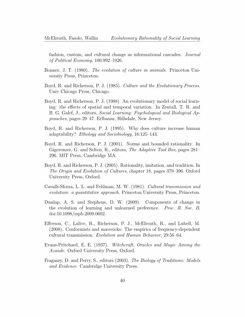
McElreath, Fasolo, Wallin Evolutionary Rationality of Social Learning
fashion, custom, and cultural change as informational cascades. Journalof Political Economy, 100:992–1026.
Bonner, J. T. (1980). The evolution of culture in animals. Princeton Uni-versity Press, Princeton.
Boyd, R. and Richerson, P. J. (1985). Culture and the Evolutionary Process.Univ Chicago Press, Chicago.
Boyd, R. and Richerson, P. J. (1988). An evolutionary model of social learn-ing: the effects of spatial and temporal variation. In Zentall, T. R. andB. G. Galef, J., editors, Social Learning: Psychological and Biological Ap-proaches, pages 29–47. Erlbaum, Hillsdale, New Jersey.
Boyd, R. and Richerson, P. J. (1995). Why does culture increase humanadaptability? Ethology and Sociobiology, 16:125–143.
Boyd, R. and Richerson, P. J. (2001). Norms and bounded rationality. InGigerenzer, G. and Selten, R., editors, The Adaptive Tool Box, pages 281–296. MIT Press, Cambridge MA.
Boyd, R. and Richerson, P. J. (2005). Rationality, imitation, and tradition. InThe Origin and Evolution of Cultures, chapter 18, pages 379–396. OxfordUniversity Press, Oxford.
Cavalli-Sforza, L. L. and Feldman, M. W. (1981). Cultural transmission andevolution: a quantitative approach. Princeton University Press, Princeton.
Dunlap, A. S. and Stephens, D. W. (2009). Components of change inthe evolution of learning and unlearned preference. Proc. R. Soc. B,doi:10.1098/rspb.2009.0602.
Efferson, C., Lalive, R., Richerson, P. J., McElreath, R., and Lubell, M.(2008). Conformists and mavericks: The empirics of frequency-dependentcultural transmission. Evolution and Human Behavior, 29:56–64.
Evans-Pritchard, E. E. (1937). Witchcraft, Oracles and Magic Among theAzande. Oxford University Press, Oxford.
Fragaszy, D. and Perry, S., editors (2003). The Biology of Traditions: Modelsand Evidence. Cambridge University Press.
40

McElreath, Fasolo, Wallin Evolutionary Rationality of Social Learning
Galef, B. G. (1992). The question of animal culture. Human Nature,3(2):157–178.
Galef, B.G., J. (1996). Social enhancement of food preferences in norway rats:A brief review. In Social Learning and Imitation: The Roots of Culture.
Gillespie, J. H. (1974). Natural selection for within-generation variance inoffspring number. Genetics, 76:601–606.
Gillespie, J. H. (1994). The Causes of Molecular Evolution. Oxford UniversityPress, Oxford.
Gintis, H. (2000). Game Theory Evolving. Princeton University Press,Princeton.
Giraldeau, L.-A. and Caraco, T. (2000). Social foraging theory. PrincetonUniversity Press, Princeton.
Henrich, J. (2001). Cultural transmission and the diffusion of innovations:Adoption dynamics indicate that biased cultural transmission is the pre-dominate force in behavioral change and much of sociocultural evolution.American Anthropologist, 103:992–1013.
Henrich, J. and Boyd, R. (1998). The evolution of conformist transmissionand the emergence of between-group differences. Evolution and HumanBehavior, 19:215–242.
Henrich, J. and Boyd, R. (2001). Why people punish defectors: Weak con-formist transmission can stabilize costly enforcement of norms in cooper-ative dilemmas. Journal of Theoretical Biology, 208:79–89.
Henrich, J. and Gil-White, F. (2001). The evolution of prestige: Freelyconferred status as a mechanism for enhancing the benefits of culturaltransmission. Evolution and Human Behavior, 22:165–196.
Henrich, J. and McElreath, R. (2003). The evolution of cultural evolution.Evolutionary Anthropology, 12:123–135.
Hill, K. and Kintigh, K. (2009). Can anthropologists distinguish good andpoor hunters: Implications for hunting hypotheses, sharing conventions,and cultural transmission. Current Anthropology.
41
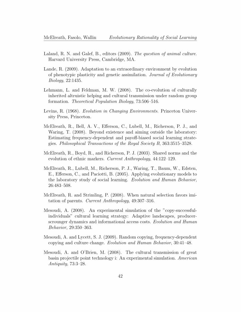
McElreath, Fasolo, Wallin Evolutionary Rationality of Social Learning
Laland, R. N. and Galef, B., editors (2009). The question of animal culture.Harvard University Press, Cambridge, MA.
Lande, R. (2009). Adaptation to an extraordinary environment by evolutionof phenotypic plasticity and genetic assimilation. Journal of EvolutionaryBiology, 22:1435.
Lehmann, L. and Feldman, M. W. (2008). The co-evolution of culturallyinherited altruistic helping and cultural transmission under random groupformation. Theoretical Population Biology, 73:506–516.
Levins, R. (1968). Evolution in Changing Environments. Princeton Univer-sity Press, Princeton.
McElreath, R., Bell, A. V., Efferson, C., Lubell, M., Richerson, P. J., andWaring, T. (2008). Beyond existence and aiming outside the laboratory:Estimating frequency-dependent and payoff-biased social learning strate-gies. Philosophical Transactions of the Royal Society B, 363:3515–3528.
McElreath, R., Boyd, R., and Richerson, P. J. (2003). Shared norms and theevolution of ethnic markers. Current Anthropology, 44:122–129.
McElreath, R., Lubell, M., Richerson, P. J., Waring, T., Baum, W., Edsten,E., Efferson, C., and Paciotti, B. (2005). Applying evolutionary models tothe laboratory study of social learning. Evolution and Human Behavior,26:483–508.
McElreath, R. and Strimling, P. (2008). When natural selection favors imi-tation of parents. Current Anthropology, 49:307–316.
Mesoudi, A. (2008). An experimental simulation of the ”copy-successful-individuals” cultural learning strategy: Adaptive landscapes, producer-scrounger dynamics and informational access costs. Evolution and HumanBehavior, 29:350–363.
Mesoudi, A. and Lycett, S. J. (2009). Random copying, frequency-dependentcopying and culture change. Evolution and Human Behavior, 30:41–48.
Mesoudi, A. and O’Brien, M. (2008). The cultural transmission of greatbasin projectile point technology i: An experimental simulation. AmericanAntiquity, 73:3–28.
42
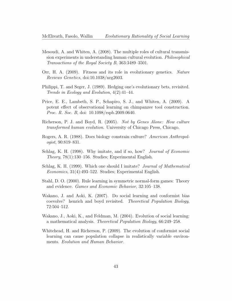
McElreath, Fasolo, Wallin Evolutionary Rationality of Social Learning
Mesoudi, A. and Whiten, A. (2008). The multiple roles of cultural transmis-sion experiments in understanding human cultural evolution. PhilosophicalTransactions of the Royal Society B, 363:3489–3501.
Orr, H. A. (2009). Fitness and its role in evolutionary genetics. NatureReviews Genetics, doi:10.1038/nrg2603.
Philippi, T. and Seger, J. (1989). Hedging one’s evolutionary bets, revisited.Trends in Ecology and Evolution, 4(2):41–44.
Price, E. E., Lambeth, S. P., Schapiro, S. J., and Whiten, A. (2009). Apotent effect of observational learning on chimpanzee tool construction.Proc. R. Soc. B, doi: 10.1098/rspb.2009.0640.
Richerson, P. J. and Boyd, R. (2005). Not by Genes Alone: How culturetransformed human evolution. University of Chicago Press, Chicago.
Rogers, A. R. (1988). Does biology constrain culture? American Anthropol-ogist, 90:819–831.
Schlag, K. H. (1998). Why imitate, and if so, how? Journal of EconomicTheory, 78(1):130–156. Studies; Experimental English.
Schlag, K. H. (1999). Which one should I imitate? Journal of MathematicalEconomics, 31(4):493–522. Studies; Experimental English.
Stahl, D. O. (2000). Rule learning in symmetric normal-form games: Theoryand evidence. Games and Economic Behavior, 32:105–138.
Wakano, J. and Aoki, K. (2007). Do social learning and conformist biascoevolve? henrich and boyd revisited. Theoretical Population Biology,72:504–512.
Wakano, J., Aoki, K., and Feldman, M. (2004). Evolution of social learning:a mathematical analysis. Theoretical Population Biology, 66:249–258.
Whitehead, H. and Richerson, P. (2009). The evolution of conformist sociallearning can cause population collapse in realistically variable environ-ments. Evolution and Human Behavior.
43