the exponentiated gompertz generated family of...

Chilean Journal of StatisticsVol. 7, No. 2, September 2016, 29-50

Research Paper

The Exponentiated Gompertz Generated Family ofDistributions: Properties and Applications

Gauss M. Cordeiro1, Morad Alizadeh2,∗, Abraao D. C. Nascimento1, Mahdi Rasekhi3

1Departamento de Estatıstica, Universidade Federal de Pernambuco, Recife, Brazil,2Department of Statistics, Persian Gulf University, Bushehr, Iran,

3Department of Statistics, Malayer University, Malayer, Iran,

(Received: June 21, 2016 · Accepted in final form: August 31, 2016)

Abstract

The proposal of more flexible distributions is an activity often required in practical con-texts. In particular, adding a positive real parameter to a probability distribution byexponentiation of its cumulative distribution function has provided flexible generateddistributions having interesting statistical properties. In this paper, we study generalmathematical properties of a new generator of continuous distributions with three extraparameters called the exponentiated Gompertz generated (EGG) family. We presentsome of its special models as well as an essay on its physical motivation. From math-ematical point of view, we derive explicit expressions of the EGG family: the ordinaryand incomplete moments, quantile and generating functions, Bonferroni and Lorenzcurves, Shannon and Renyi entropies and order statistics, which are valid for any base-line model. We also provide a bivariate EGG extension. The estimation procedure bymaximum likelihood of the new class is elaborated and discussed. In order to quantifyand to assess the asymptotic behavior of this procedure, we perform a simulation study.Finally, two applications to real data are performed. Results furnish evidence in favorof the use of the EGG beta distribution as a good proposal to these data sets.

Keywords: Reliability and life testing · Applications to social sciences · Gompertzdistribution · New generator · New Distribution for proportion.

1. Introduction

In many practical situations, classical distributions do not provide adequate fits to realdata. Thus, several generators of introducing one or more parameters to generate newdistributions have been proposed in the statistical literature. Some well known generatorsare

• Marshal-Olkin generated family (MO-G) (Marshall and Olkin, 1997),

• the beta-G by Eugene et al. (2002) and Jones (2004), Kumaraswamy-G (Kw-G for short)by Cordeiro and de Castro (2011) and McDonald-G (Mc-G) by Alexander et al. (2012),

• gamma-G (type 1) by Zografos and Balakrishnan (2009), gamma-G (type 2) by Risticand Balakrishnan (2012), gamma-G (type 3) by Torabi and Hedesh (2012) and log-gamma-G by Amini et al. (2012),

∗Corresponding author. Email: [email protected]

ISSN: 0718-7912 (print)/ISSN: 0718-7920 (online)c© Chilean Statistical Society - Sociedad Chilena de Estadısticahttp://www.soche.cl/chjs

30 Cordeiro, Alizadeh, Nascimento and Rasekhi

• logistic-G by Torabi and Montazeri (2012),

• exponentiated generalized-G by Cordeiro et al. (2011),

• Transformed-Transformer (T-X) by Alzaatreh et al. (2013) and exponentiated (T-X) byAlzaghal et al. (2013),

• Weibull-G by Bourguignon et al. (2014) and

• Exponentiated half logistic generated family by Cordeiro et al. (2014).

In general, all above classes can be expressed within one formulation as follows.Let r(t) be the probability density function (pdf) of the random variable T ∈ [a, b] for−∞ < a < b < ∞ and W [G(x)] be the cumulative distribution function (cdf) of therandom variable X, satisfying the following conditions:

(i) W [G(x)] ∈ [a, b],(ii) W [G(x)] is differentiable and monotonically non-decreasing, and(iii) W [G(x)]→ a as x→ −∞ andW [G(x)]→ b as x→∞.

Recently, Alzaatreh et al. (2013) defined the T-X family of distributions by

F (x) =

∫ W [G(x)]

ar(t) dt, (1)

where W [G(x)] satisfies the conditions (i)–(iii). The pdf obtained from (1) is given by

f(x) =

{d

dxW [G(x)]

}r {W [G(x)]} . (2)

In the remainder of this paper, we introduce a new class from (1) and study some of itsstatistical properties.

El-Gohary et al. (2013) defined the three-parameter generalized Gompertz (GG) distri-bution having pdf and cdf given by

π(x ; θ, γ, α) = α θ eγ x e−θ

γ( eγ x− 1 )

[1 − e−

θ

γ( eγ x− 1 )

]α− 1

and

Π(x ; θ, γ, α) =[

1 − e−θ

γ( eγ x− 1 )

]α,

respectively, where x, θ, γ, α > 0. Notice that the GG model colapses in the Gompertz (G)distribution when α = 1. Now, applying (i) W [G(x)] = − log[1−G(x)] and (ii)

r(t) = α θ eγ t e−θ

γ( eγ t− 1 )

[1 − e−

θ

γ( eγ t− 1 )

]α− 1, t > 0,

on (2), we define a new family of distributions–called the exponentiated Gompertz generated(“EGG” for short) family– having cdf expressed in the form of the next theorem.

Theorem 1.1 The cdf of the EGG family is given by

F (x ; θ, γ, α, ξ) =

∫ − log[ 1−G(x ; ξ) ]

0π(w ; θ, γ, α) dw =

{1− e

θ

γ{ 1− [ 1−G(x ; ξ) ]−γ }

}α,

(3)where θ > 0, γ > 0 and α > 0 are three extra shape parameters.

Chilean Journal of Statistics 31

Equation (3) is a wider family of continuous distributions. It includes several classes suchas the proportional hazard rate distributions (Gupta and Gupta, 2007). For each baselineG, the EGG-G distribution is defined by the cdf (3). Henceforth, X ∼ EGG-G(θ, γ, α, ξ)denotes a random variable having the cdf (3) and G(x ; ξ) denotes the baseline cdf de-pending on a parameter vector ξ. For simplicity, we can omit the dependence on ξ andwrite simply G(x) = G(x; ξ).

A probabilistic deduction and physical interpretation of the EGG family can be ad-dressed as follows. Let Y be a random variable having the Gompertz distribution (withpositive parameters θ and γ representing the shape and scale, respectively) and Z beany random variable with baseline cdf G(z; ξ). Thus, if we consider α systems, T1, . . . , Tαworking independently as a random sample from T • = G−1(1 − e−Y ; ξ), then the cdf ofX = max{T1, . . . , Tα} given by

Pr(X ≤ x) = Pr(∩αi=1 {Xi ≤ x}) = {Pr( {X1 ≤ x})}α

= {Pr(G−1(1− e−Y ; ξ) ≤ x )}α

= {Pr(Y ≤ − log[ 1 − G(x; ξ) ] ) }α

= F (x ; θ, γ, α, ξ),

follows the proposed family. In other words, this property characterizes the distribution ofthe maximum of α random variables having the G distribution (with parameter vector ξ)such that their cdf’s are defined by 1 − e−Y , where Y has the Gompertz(θ, γ) distribu-tion. Applications in several areas can be associated to the above discussion, such those inreliability and anthropological contexts. Consider a system formed by α independent com-ponents following specific transformed distribution involving the Gompertz and a baselineG model. Suppose the system fails if all of the α components fail. Let T1, . . . , Tα denote thelifetimes. Thus, X describes the maximum lifetime under the influence of the parametersα, θ, γ and ξ.

This paper is organized as follows. In Section 2, we provide the EGG density and quantilefunctions. Three special cases of the proposed family are addressed in Section 3. Someuseful expansions are derived in Section 4. A power series expansion for the quantilefunction (qf) of X is derived in Section 5. In Section 6, we provide explicit expressions forthe moments and generating function of X. In Section 7, we present general expressionsfor the Renyi and Shannon entropies. In Section 8, the order statistics are investigated. InSection 9, we introduce a bivariate extension of the new family. Estimation of the modelparameters by maximum likelihood is performed in Section 10. A simulation study andtwo applications to real data illustrate the usefulness of the EGG family in Section 12.The paper is concluded in Section 13.

2. The new family

The pdf and hrf corresponding to (3) are provided in the corollary:

Corollary 2.1 The pdf and hrf of X are given by

f(x ; θ, γ, α, ξ) =α θ g(x ; ξ) e

θ

γ{ 1− [ 1−G(x ; ξ) ]−γ }

[ 1 − G(x ; ξ) ]1 + γ

{1 − e

θ

γ{ 1− [ 1−G(x ; ξ) ]−γ }

}α− 1,

(4)


and

h(x ; θ, γ, α, ξ) =θ g(x ; ξ)

[ 1 − G(x ; ξ) ]γ+ 1

{1 − e

θ

γ{ 1− [ 1−G(x ; ξ) ]−γ }

}α− 1[1 −

{1 − e

θ

γ{ 1− [ 1−G(x ; ξ) ]−γ }

}α] , (5)

respectively, where x ∈ X and g(x ; ξ) is the baseline pdf.

A simple pdf (4) arises when one considers simple expressions for G(x) and g(x). As theEGG family can be understood as a “dictionary” of special models, an other practical issueis “how to select the more appropriate baseline for a data set?”. In practice, the followingcriteria are often used: (i) take into account the variation range of real data and/or (ii)choose one parent distribution among many others models based on the smaller valueassumed by the sum of squablack errors between the histogram and the fitted densityf(x ; θ, γ, α, ξ) as discussed by Cintra et al. (2013), where θ, γ, α and ξ are obtained byany estimation method, usually maximum likelihood.

The EGG family of distributions is easily simulated by inverting (3) as follows: if u isan outcome from the uniform U(0, 1) distribution, then

x = QG

{1−

[1− γ

θlog(1− u

1

α )]−1

γ

}, (6)

is an outcome of a random variable X having pdf (4), where QG(x) = G−1(x) is the qf ofG.

Figure 1 displays the qf’s of X taking the normal N(µ, σ2) and beta B(β1, β2) models asthe parent distributions. These situations are detailed in the next section.

0.0 0.2 0.4 0.6 0.8 1.0

01

23

45

6

Probability

Qua

ntile

func

tion

k = 2k = 1k = 1 2k = 1 4

(a) (θ, γ, α) = (1, 1, 1) and µ = σ = k

0.0 0.2 0.4 0.6 0.8 1.0

0.0

0.2

0.4

0.6

0.8

1.0

Probability

Qua

ntile

func

tion

k = 2k = 1k = 1 2k = 1 4

(b) (θ, γ, α) = (1, 1, 1) and β1 = β2 = k

Figure 1. Plots of the EGG qf’s for the N(µ, σ2) and B(β1, β2) baselines.

3. Some Special EGG distributions

For α = 1, we obtain as a special case of (4) the Gompertz-G family of distributions (Al-izadeh et al., 2016). The exponentiated class of distributions proposed by Cordeiro et al.(2016) arises as another special case when γ ↓ 0. For γ ↓ 0 and α = 1, equation (4) re-duces to the Gupta and Gupta’s proportional hazard rate class (Gupta and Gupta, 2007).For γ ↓ 0 and θ = 1, we have the reversed hazard rate class (Gupta and Gupta, 2007),


which provides greater flexibility of its tails and can be widely applied in many areas ofengineering and biology. Some special models are listed in Table 1.

This table indicates that the hypotheses H0 : α = 1 and γ ↓ 0, H0 : θ = 1 and γ ↓ 0 andH0 : θ = α = 1 and γ ↓ 0 can be used when one wishes to assess an extension of the classproposed by Alizadeh et al. (2016), a change of the proportional hazard rate model in theform of the parameter θ and the influence of the new class on the baseline distribution,respectively. Next, we present three special cases of the EGG family, where γ > 0, θ > 0and α > 0.

Table 1. Some special models

α θ γ G(x) family

1 - - - Gompertz-G family of distributions (Alizadeh et al., 2016)

- - ↓ 0 - Exponentiated class of distributions (Cordeiro et al., 2016)

1 - ↓ 0 - Proportional hazard rate model (Gupta and Gupta, 2007)

- 1 ↓ 0 - Proportional reversed hazard rate model (Gupta and Gupta, 2007)

1 1 ↓ 0 - G(x)

1 - - 1 − e−x Gompertz distribution

- - - 1 − e−x Generalized Gompertz distribution (El-Gohary et al., 2013)

1 - ↓ 0 xv Kumaraswamy distribution (Kumaraswamy, 1980; Jones, 2009)

- - ↓ 0 xv Exponentiated Kumaraswamy distribution and its log transform

(Lemonte et al., 2013)

3.1 The EGGN distribution

We define the exponentiated Gompertz generated normal (EGGN) distribution from (4) bytaking G(x ; ξ) = Φ(x−µσ ) and g(x ; ξ) = σ−1 φ(x−µσ ) to be the cdf and pdf of the normaldistribution with parameters µ and σ2, respectively, ξ = (µ, σ2), and where φ(·) and Φ(·)are the pdf and cdf of the standard normal distribution, respectively. Then, the EGGNpdf is given by

f(x ; θ, γ, α, µ, σ) =α θ

σφ(x− µ

σ

) [1 − Φ

(x− µσ

) ]−γ−1eθ

γ { 1− [ 1−Φ( x−µσ

) ]−γ }

×{

1 − eθ

γ{ 1− [ 1−Φ( x−µ

σ)]−γ }

}α−1, (7)

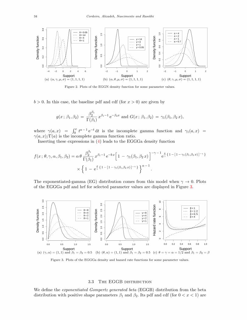
where x ∈ R, µ ∈ R is a location parameter and σ > 0 is a scale parameter. The randomvariable with pdf (7) is denoted by X ∼ EGGN (θ, γ, α, µ, σ2). For µ = 0, σ = 1 andγ → 0, we have the power-normal (PN) distribution (Gupta and Gupta, 2008). Further,the basic exemplar when θ = 1 and γ → 0 is the normal distribution. Plots of the EGGNdensity function for some shape parameter values are displayed in Figure 2. These plotsindicate that decreasing α and γ causes a flattening of the density curves, whereas thisbehavior happens under increasing θ (for θ > 1).

3.2 The EGGGa distribution

We also present as a special model the exponentiated Gompertz generated gamma (EGGGa)distribution from the gamma distribution with shape parameter a > 0 and scale parameter


−4 −2 0 2 4 6

0.0

0.2

0.4

0.6

0.8

Support

Den

sity

func

tion

θ = 0.05θ = 14θ = 4θ = 1

(a) (α, γ, µ, σ) = (1, 1, 1, 1)

−2 −1 0 1 2

0.0

0.5

1.0

1.5

Support

Den

sity

func

tion

γ = 14γ = 4γ = 1γ = 0.05

(b) (α, θ, µ, σ) = (1, 1, 1, 1)

−2 −1 0 1 2

0.0

0.2

0.4

0.6

0.8

1.0

Support

Den

sity

func

tion

α = 4α = 2α = 1α = 0.7

(c) (θ, γ, µ, σ) = (1, 1, 1, 1)

Figure 2. Plots of the EGGN density function for some parameter values.

b > 0. In this case, the baseline pdf and cdf (for x > 0) are given by

g(x ; β1, β2) =ββ1

2

Γ(β1)xβ1−1 e−β2x and G(x ; β1, β2) = γ1(β1, β2 x),

where γ(a, x) =∫ x

0 ta− 1 e−t dt is the incomplete gamma function and γ1(a, x) =γ(a, x)/Γ(a) is the incomplete gamma function ratio.

Inserting these expressions in (4) leads to the EGGGa density function

f(x ; θ, γ, α, β1, β2) = α θββ1

2

Γ(β1)xβ1−1 e−b x

[1 − γ1(β1, β2 x)

]−γ− 1eθ

γ{ 1− [ 1− γ1(β1,β2 x) ]−γ }

×{

1 − eθ

γ{ 1− [ 1− γ1(β1,β2 x) ]−γ }

}α− 1.

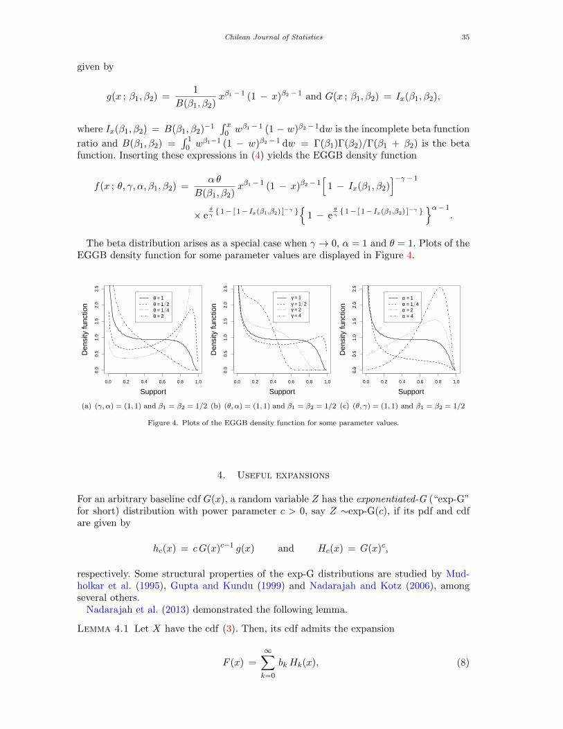
The exponentiated-gamma (EG) distribution comes from this model when γ → 0. Plotsof the EGGGa pdf and hrf for selected parameter values are displayed in Figure 3.

0.0 0.5 1.0 1.5

0.0

0.5

1.0

1.5

2.0

2.5

3.0

Support

Den

sity

func

tion θ = 8

θ = 4θ = 2θ = 1

(a) (γ, α) = (1, 1) and β1 = β2 = 0.5

0.0 0.5 1.0 1.5

0.0

0.5

1.0

1.5

2.0

2.5

3.0

Support

Den

sity

func

tion

γ = 8γ = 4γ = 2γ = 1

(b) (θ, α) = (1, 1) and β1 = β2 = 0.5

0.0 0.2 0.4 0.6 0.8 1.0

02

46

810

Support

Haz

ard

rate

func

tion

β = 1β = 1 2β = 6 5β = 4

(c) θ = γ = α = 1/2 and β1 = β2 = β

Figure 3. Plots of the EGGGa density and hazard rate functions for some parameter values.

3.3 The EGGB distribution

We define the exponentiated Gompertz generated beta (EGGB) distribution from the betadistribution with positive shape parameters β1 and β2. Its pdf and cdf (for 0 < x < 1) are


given by

g(x ; β1, β2) =1

B(β1, β2)xβ1− 1 (1 − x)β2− 1 and G(x ; β1, β2) = Ix(β1, β2),

where Ix(β1, β2) = B(β1, β2)−1∫ x

0 wβ1− 1 (1 − w)β2− 1dw is the incomplete beta function

ratio and B(β1, β2) =∫ 1

0 wβ1−1 (1 − w)β2− 1 dw = Γ(β1)Γ(β2)/Γ(β1 + β2) is the betafunction. Inserting these expressions in (4) yields the EGGB density function

f(x ; θ, γ, α, β1, β2) =α θ

B(β1, β2)xβ1− 1 (1 − x)β2− 1

[1 − Ix(β1, β2)

]−γ− 1

× eθ

γ{ 1− [ 1− Ix(β1,β2) ]−γ }

{1 − e

θ

γ{ 1− [ 1− Ix(β1,β2) ]−γ }

}α− 1.

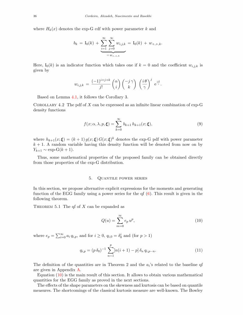
The beta distribution arises as a special case when γ → 0, α = 1 and θ = 1. Plots of theEGGB density function for some parameter values are displayed in Figure 4.

0.0 0.2 0.4 0.6 0.8 1.0

0.0

0.5

1.0

1.5

2.0

2.5

Support

Den

sity

func

tion

θ = 1θ = 1 2θ = 1 4θ = 2

(a) (γ, α) = (1, 1) and β1 = β2 = 1/2

0.0 0.2 0.4 0.6 0.8 1.0

0.0

0.5

1.0

1.5

2.0

2.5

Support

Den

sity

func

tion

γ = 1γ = 1 2γ = 2γ = 4

(b) (θ, α) = (1, 1) and β1 = β2 = 1/2

0.0 0.2 0.4 0.6 0.8 1.0

0.0

0.5

1.0

1.5

2.0

2.5

Support

Den

sity

func

tion

α = 1α = 1 4α = 2α = 4

(c) (θ, γ) = (1, 1) and β1 = β2 = 1/2

Figure 4. Plots of the EGGB density function for some parameter values.

4. Useful expansions

For an arbitrary baseline cdf G(x), a random variable Z has the exponentiated-G (“exp-G”for short) distribution with power parameter c > 0, say Z ∼exp-G(c), if its pdf and cdfare given by

hc(x) = cG(x)c−1 g(x) and Hc(x) = G(x)c,

respectively. Some structural properties of the exp-G distributions are studied by Mud-holkar et al. (1995), Gupta and Kundu (1999) and Nadarajah and Kotz (2006), amongseveral others.

Nadarajah et al. (2013) demonstrated the following lemma.

Lemma 4.1 Let X have the cdf (3). Then, its cdf admits the expansion

F (x) =

∞∑k=0

bkHk(x), (8)


where Hk(x) denotes the exp-G cdf with power parameter k and

bk = I0(k) +

∞∑i=1

∞∑j=0

wi,j,k︸︷︷︸=w+,+,k

= I0(k) + w+,+,k.

Here, I0(k) is an indicator function which takes one if k = 0 and the coefficient wi,j,k isgiven by

wi,j,k =(−1)i+j+k

j!

(α

i

)(−j γk

) (i θ

γ

)jei θ

γ .

Based on Lemma 4.1, it follows the Corollary 3.

Corollary 4.2 The pdf of X can be expressed as an infinite linear combination of exp-Gdensity functions

f(x;α, λ, p, ξ) =

∞∑k=0

bk+1 hk+1(x; ξ), (9)

where hk+1(x; ξ) = (k + 1) g(x; ξ)G(x; ξ)k denotes the exp-G pdf with power parameterk + 1. A random variable having this density function will be denoted from now on byYk+1 ∼ exp-G(k + 1).

Thus, some mathematical properties of the proposed family can be obtained directlyfrom those properties of the exp-G distribution.

5. Quantile power series

In this section, we propose alternative explicit expressions for the moments and generatingfunction of the EGG family using a power series for the qf (6). This result is given in thefollowing theorem.

Theorem 5.1 The qf of X can be expanded as

Q(u) =

∞∑m=0

ep up, (10)

where ep =∑∞

i=0 ai qi,p, and for i ≥ 0, qi,0 = δi0 and (for p > 1)

qi,p = (p δ0)−1p∑

n=1

[n(i+ 1)− p] δn qi,p−n. (11)

The definition of the quantities are in Theorem 2 and the ai’s related to the baseline qfare given in Appendix A.

Equation (10) is the main result of this section. It allows to obtain various mathematicalquantities for the EGG family as proved in the next sections.

The effects of the shape parameters on the skewness and kurtosis can be based on quantilemeasures. The shortcomings of the classical kurtosis measure are well-known. The Bowley


skewness (Kenney and Keeping, 1962, pp. 101–102) is one of the earliest skewness measuresdefined by the average of the quartiles minus the median, divided by half the interquartilerange, namely

B =Q(

34

)+Q

(14

)− 2Q

(12

)Q(

34

)−Q

(14

) .

Since only the middle two quartiles are consideblack and the outer two quartiles are ig-noblack, this adds robustness to the measure. The Moors kurtosis (Moors, 1998) is basedon octiles

M =Q(

38

)−Q

(18

)+Q

(78

)−Q

(58

)Q(

68

)−Q

(28

) .

From the last two equations, the skewness and kurtosis measures can be determined asfunctions of the qf of X in equation (6). These measures are less sensitive to outliersand they exist even for distributions without moments. Figure 5 displays the plots of themeasures B and M for the EGGB distribution discussed in Section 3. These plots indicatethat both measures B and M depend very much on the shape parameters.

0 1 2 3 4 5

−0.

50.

00.

51.

0

α

Ske

wne

ss M

easu

re

k = 1 4k = 1 2k = 1k = 2

(a) BEGGB: (θ, γ, α, β1, β2) = (k, k, •, 1, 1)

0 1 2 3 4 5

0.8

1.0

1.2

1.4

1.6

1.8

α

Kur

tosi

s M

easu

re

k = 1 4k = 1 2k = 1k = 2

(b) MEGGN: (θ, γ, α, β1, β2) = (k, k, •, 1, 1)

Figure 5. Plots of the skewness and kurtosis measures for the EGGB distribution.

6. Moments and generating function

Let Yk+1 be a random variable having the exp-G distribution with power parameter k+ 1,i.e., with density hk+1(x). A first formula for the nth moment of X follows from (9) as

E(Xn) =

∞∑k=0

bk+1 E(Y nk+1). (12)

Expressions for moments of several exp-G distributions are given by Nadarajah and Kotz(2006), which can be used to obtain E(Xn).

A second formula for E(Xn) can be expressed from (12) in terms of the G qf as

E(Xn) =

∞∑k=0

(k + 1) bk+1 τ(n, k), (13)


where τ(n, k) =∫∞−∞ x

nG(x)k g(x) dx =∫ 1

0 QG(u)n uadu. Cordeiro and Nadarajah (2011)obtained the quantity τ(n, k) for some well-known models such as the normal, beta, gammaand Weibull distributions.

We now move to the nth incomplete moment of X defined by mn(y) = E(Xn|X < y) =∫ y−∞ x

r f(x) dx. For empirical purposes, the shape of many distributions can be usefullydescribed by what we call the incomplete moments. These types of moments play animportant role for measuring inequality, for example, income quantiles and Lorenz andBonferroni curves, which depend upon the incomplete moments. The quantity mn(y) canbe expressed as

mn(y) = E(Xn|X < y) =

∞∑k=0

(k + 1) bk+1

∫ G(y;ξ)

0QG(u)n ukdu. (14)

The integral in equation (14) can be computed at least numerically for most baselinedistributions. A second method to obtain the incomplete moments of X follows from (14)using equations (A5) and (A6):

Corollary 6.1 The nth incomplete of X is given by

mn(y) =

∞∑k,m=0

(k + 1) bk+1 cn,m(m+ k + 1)

G(y; ξ)m+k+1, (15)

where the coefficients cn,m can be determined by (A6).

Let MX(t) = E(et X) be the moment generating function (mgf) of X. A first expressionfor MX(t) comes from (9) as

MX(t) =

∞∑k=0

bk+1Mk+1(t), (16)

where Mk+1(t) is the mgf of Yk+1. Hence, MX(t) can be determined from the exp-Ggenerating function.

A second formula for M(t) can be derived from (9) as

M(t) =

∞∑i=0

(k + 1) bk+1 ρ(t, k), (17)

where ρ(t, k) =∫∞−∞ et x G(x)k g(x)dx =

∫ 10 exp[t QG(u)] uk du.

We can obtain the mgfs of several distributions directly from equations (16) and (17).

7. Entropies

An entropy is a measure of variation or uncertainty of a random variable X. Two popularentropy measures are the Renyi and Shannon entropies (Shannon, 1948; Renyi, 1961). TheRenyi entropy of a random variable with pdf f(x) is defined as

IR(c) =1

1− clog

(∫ ∞0

f c(x) dx

),


for c > 0 and c 6= 1. The Shannon entropy of a random variable X is defined byE {− log [f(X)]}. It is the special case of the Renyi entropy when c ↑ 1. Direct calcu-lation yields:

Corollary 7.1 The Shannon entropy of X is given by

E {− log[f(X)]} = − log(αθ)− E {log[g(X; ξ)]}

+(γ + 1)αθ

γ2

∞∑i,j=0

(−1)i+j+1

(j + 1) (j + 1)!

(α− 1

i

)[(i+ 1)θ

γ

]je

(i+1)θ

γ

− θγ

1− αθ

γ2

∞∑i,j=0

(−1)i+j

(j + 2) j!

(α− 1

i

)[(i+ 1)θ

γ

]j e(i+1)θ

γ

−α(α− 1)θ

γ

∞∑i,j=0

(−1)i+j+1

(j + 1)!

[(i+ 1)θ

γ

]je

(i+1)θ

γ

[ ∂∂t

(t+ α− 1

i

)∣∣∣t=0

].

After some algebraic developments, we can obtain an alternative expression for IR(c).

Corollary 7.2 The Renyi’s entropy of X is given by

IR(c) =c

1− clog(αθ) +

1

1− clog

∞∑i,j,k

mi,j,k I(c, k)

(18)

where

mi,j,k =

(−1)i+j+k(c(α− 1)

i

)eθ(c+i)

γ (θ(c+ i))j(−c(γ + 1) − γ j

k

)j! γj

and

I(c, k) =

∫ ∞−∞

g(x)cG(x)k dx

8. Order statistics

Order statistics make their appearance in many areas of statistical theory and practice.Suppose X1, . . . , Xn is a random sample from the EGG-G family of distributions. Let Xi:n

denote the ith order statistic. The pdf of Xi:n can be expressed as

fi:n(x) =K f(x)F i−1(x) {1− F (x)}n−i

=K

n−i∑j=0

(−1)j(n− ij

)f(x)F (x)j+i−1,

where K = n!/[(i− 1)! (n− i)!].We can demonstrate that the density function of the ith order statistic of any EGG-G

distribution follows Corollary 6.

Corollary 8.1 Let X1, . . . , Xn be a random sample from X ∼ EGG(θ, γ, α, ξ), The pdf


of Xi:n can be expressed as

fi:n(x) =

∞∑r,k=0

n−i∑j=0

mj,r,k hr+k+1(x), (19)

where hr+k(x) denotes the exp-G density function with power parameter r + k,

mj,r,k =(−1)j n!

(i− 1)! (n− i− j)! j!(r + 1) br+1 fj+i−1,k

[r + k + 1], (20)

and bk is given by (8). Here, the quantity fj+i−1,k is obtained recursively from fj+i−1,0 =

bj+i−10 and (for k ≥ 1)

fj+i−1,k = (k b0)−1k∑

m=1

[m(j + i)− k] bm fj+i−1,k−m.

So, we can easily obtain the ordinary and incomplete moments and generating functionfor the EGG-G order statistics (based on any G distribution) from equation (19).

9. Bivariate extension

A bivariate extension is presented in the following theorem.

Theorem 9.1

F (x, y ; ξ) ={

1 − eθ

γ{ 1− [ 1−G(x,y ; ξ) ]−γ }

}α,

where G(x, y ; ξ) is a bivariate continuous distribution with marginal cdf’sG1(x ; ξ) and G2(y; ξ). The marginal cdf’s are given by

FX(x ; ξ) ={

1 − eθ

γ{ 1− [ 1−G(x ; ξ) ]−γ }

}αand

FY (y ; ξ) ={

1 − eθ

γ{ 1− [ 1−G(y ; ξ) ]−γ }

}α.

The joint pdf of (X,Y ) is easily determined by fX,Y (x, y) = ∂2FX,Y (x, y)/∂x ∂y:

Corollary 9.2

fX,Y (x, y) =α θ [ 1 − G(x, y ; ξ) ]−γ− 1 eθ

γ{ 1− [ 1−G(x,y ; ξ) ]−γ }

× A(x, y ; ξ){

1 − eθ

γ{ 1− [ 1−G(x,y ; ξ) ]−γ }

}α− 1,


where

A(x, y ; ξ) = g(x, y ; ξ) −

[γ + 1

1 − G(x, y ; ξ)

][∂G(x, y ; ξ)

∂x

] [∂G(x, y ; ξ)

∂y

]

− θ

[ 1 − G(x, y ; ξ) ]γ+ 1

[∂G(x, y ; ξ)

∂x

] [∂G(x, y ; ξ)

∂y

]

+θ (α − 1)

[ 1 − G(x, y ; ξ) ]γ+ 1

eθ

γ{ 1− [ 1−G(x,y ; ξ) ]−γ }

1 − eθ

γ{ 1− [ 1−G(x,y ; ξ) ]−γ }

[∂G(x, y ; ξ)

∂x

] [∂G(x, y ; ξ)

∂y

].

The marginal pdf’s are

fX(x ; θ, γ, α, ξ) =α θ g1(x ; ξ) [ 1 − G1(x; ξ)]−γ− 1 eθ

γ{ 1− [ 1−G1(x ; ξ) ]−γ }

×{

1 − eθ

γ{ 1− [ 1−G1(x ; ξ) ]−γ }

}α− 1

and

fY (y ; θ, γ, α, ξ) =α θ g2(y ; ξ) [ 1 − G2(y ; ξ) ]−γ− 1 eθ

γ{ 1− [ 1−G2(y ; ξ) ]−γ }

×{

1 − eθ

γ{ 1− [ 1−G2(y ; ξ) ]−γ }

}α− 1.

The conditional density functions are

f(x | y) =[1−G(x, y; ξ)]−γ−1e

θ

γ{1−[1−G(x,y;ξ)]−γ}A(x, y; ξ)

{1− e

θ

γ{1−[1−G(x,y;ξ)]−γ}

}α−1

g2(y; ξ)[1−G2(y; ξ)]−γ−1eθ

γ{1−[1−G2(y;ξ)]−γ}

{1− e

θ

γ{1−[1−G2(y;ξ)]−γ}

}α−1

and

f(y | x) =[1−G(x, y; ξ)]−γ−1e

θ

γ{1−[1−G(x,y;ξ)]−γ}A(x, y; ξ)

{1− e

θ

γ{1−[1−G(x,y;ξ)]−γ}

}α−1

g1(x; ξ)[1−G1(x; ξ)]−γ−1eθ

γ{1−[1−G1(x;ξ)]−γ}

{1− e

θ

γ{1−[1−G1(x;ξ)]−γ}

}α−1 .

10. Estimation

We determine the maximum likelihood estimates (MLEs) of the parameters of the newfamily from complete samples only. Let x1, . . . , xn be the observed values from the EGG-Gdistribution with parameters θ, γ, α and ξ. Let Θ = (θ, γ, α, ξ)> be the r × 1 parametervector. The total log-likelihood function for Θ is given by

`n = `n(Θ) = n log(α θ) +

n∑i=1

log [g(xi; ξ)]− (γ + 1)

n∑i=1

log [1−G(x ; ξ)]

+

n∑i=1

log(1− ti) + (α− 1)

n∑i=1

log(ti), (21)


where ti = 1 − eθ

γ{ 1− [ 1−G(xi ; ξ) ]−γ }.

The log-likelihood can be maximized either directly or by solving the nonlinear likelihoodequations obtained by differentiating (21). The components of the score function Un(Θ) =(∂`n/∂θ, ∂`n/∂γ, ∂`n/∂α, ∂`n/∂ξ

)>are

∂`n∂θ

=n

θ−

n∑i=1

t(θ)i

1− ti+ (α− 1)

n∑i=1

t(θ)i

ti,

∂`n∂γ

= −n∑i=1

log[1−G(xi; ξ)]−n∑i=1

t(γ)i

1− ti+ (α− 1)

n∑i=1

t(γ)i

ti,

∂`n∂α

=n

α+

n∑i=1

log(ti)

and

∂`n∂ξ

=

n∑i=1

g(ξ)(x; ξ)

g(x; ξ)+ (γ + 1)

n∑i=1

g(ξ)(x; ξ)

1−G(x; ξ)−

n∑i=1

t(ξ)i

1− ti+ (α− 1)

n∑i=1

t(ξ)i

ti,

where t(ζ)i = Cζ e

θ

γ{ 1− [ 1−G(x ; ξ) ]−γ },

Cζ =

− 1γ , if ζ = θ,

θγ2 , if ζ = γ,γ G(ξ)(x ; ξ)

[1−G(x ; ξ)]γ− 1 , if ζ = ξ

and h(ξ)(·) denotes the derivative of the function h with respect to ξ. Often with lifetimedata and reliability studies, one encounters censoring. A very simple random censoringmechanism very often realistic is one in which each individual i is assumed to have a lifetimeXi and a censoring time Ci, where Xi and Ci are independent random variables. Supposethat the data consist of n independent observations xi = min(Xi, Ci) and δi = I(Xi ≤ Ci)is such that δi = 1 if Xi is a time to event and δi = 0 if it is right censoblack for i = 1, . . . , n.The censoblack likelihood L(Θ) for the model parameters blackuces to

L(Θ) ∝n∏i=1

[f(xi; θ, γ, α, ξ)]δi [S(xi; θ, γ, α, ξ)]1−δi ,

where f(x; θ, γ, α, ξ) is given by (4) and S(x; θ, γ, α, ξ) is the survival function computedby (3).

11. Simulation study

Here, we give a simulation study in order to assess the MLEs described in Section 13. One ofadvantages of the EGG family of distributions is that its cdf has tractable analytical form.This fact implies in a simple random number generator (RNG). We use the algorithm.

(1) Generate U ∼ U(0, 1).


(2) Specify a function G(·; ·) as defined in Section 3.(3) Obtain an outcome of X by

X = G−1

(1−

[1− γ

θlog(1− U

1

α )]−1

γ

; ξ

).

The EGGB fitted density is plotted in Figure 6.

●

●

●

●

●

●

●

●

●

●

●

●●

●

●

●

●

●

●

●

●

●●

●

●

●

●

●

●

●●

●

●

●●

●

●

●

●

●

●●

●

●

●

●

●

●●

●

●

●

●

●

●

●

●

●

●

●

●

●

●

●●

●

●

●

●

●

●

●

●

●

●

●

●

●

●

●

●

●

●

●

●

●

●

●

●

●

●●●

●

●

●

●

●

●

●

0.0 0.2 0.4 0.6 0.8 1.0

0.0

0.5

1.0

1.5

2.0

2.5

Generated EGGB values

EG

GB

and

em

piric

al d

ensi

ties

Figure 6. Plots of the theoretical (black and solid), fitted (black and long dashes) and empirical (points) densityfunction for the EGGB(1/2, 1, 1, 1/2, 1/2) distribution.

We perform a simulation study in order to assess the influence of the additional param-eters (α, θ and γ) on the difference between the theoretical and fitted curves associatedwith the EGGB distribution. To that end, we consider 1,000 Monte Carlo’s replicationsand, on each replication, the mean square error (MSE) between the fitted and empiricaldensities is quantified such as a goodness-of-fit criterion. The current simulation processis conducted following the steps:

(1) Simulated EGGB distributed data of N ∈ {50, 100, 150} are obtained by means ofthe EGG RNG.

(2) Fixing the baseline vector of parameters as ξ = (β1, β2) = (1/2, 1/2) for the EGGBdistribution, respectively. Three scenarios are consideblack: (a) θ = 1/2, γ = 1 andα ∈ {1, 1.5, 2, 2.5, 3, 3.5, 4, 4.5, 5}; (b) θ = 1/2, γ ∈ {1, 1.5, 2, 2.5, 3, 3.5, 4, 4.5, 5}and α = 1; and (c) θ ∈ {1, 1.5, 2, 2.5, 3, 3.5, 4, 4.5, 5}, γ = 1 and α = 1.

(3) The generated data is submitted to the ML estimation to obtain the parameter

estimates and the estimated EGGB pdf fEGGB(·).(4) The MSEs between the exact and estimated pdfs are computed.

Figure 7 displays the relationship between the shape parameters and the MSEs. Based onthe asymptotic properties of the MLEs, the MSEs decrease when the sample size increases(as expected). It is noticeable that the estimation of the parameter θ is the most hardsituation, whereas the estimation of α is the most tractable.

In general, for a given sample size, the estimation of the EGGB extra parameters γ andα tends not to be influenced by increasing the parameter values.


●

●

●

●

●

●

●

●

●

1 2 3 4 5

01

23

θ

MS

E(θ

)

●●

●

● ●●

●

●●

●●

●●

●●

●● ●

●

●

●

N = 50N = 100N = 150

(a)

●

●

●

●●

● ●●

●

1 2 3 4 5

0.00

0.05

0.10

0.15

0.20

0.25

0.30

γ

MS

E(γ

)

● ● ●●

● ●● ● ●

● ● ● ● ● ● ●● ●

(b)

●

●●

●● ●

● ● ●

1 2 3 4 5

0.00

0.05

0.10

0.15

0.20

0.25

0.30

α

MS

E(α

)

●

● ● ● ● ●● ●

●

●

● ● ● ● ● ● ● ●

(c)

Figure 7. MSEs for some EGGB parameter values.

12. Applications

In this section, two applications to real data are performed in order to illustrate the po-tentiality of the EGGB distribution.The first application consists the total milk production in one hundred seven SINDI racecows on the first birth after to calve.These cows are property of the Carnauba farm whichbelongs to the Agropecuaria Manoel Dantas Ltda (AMDA), located in the Taperoa City,Paraiba (Brazil). The original data are not in the interval (0, 1) and it was made the

transformation given by xi = yi−min(yi)max(yi)−min(yi)

, for i = 1, ..., 107. These data are presented

in Cordeiro and Brito (2012). These data have already been used in Cordeiro and Brito(2012)presented evidence that such set of data can be well described by the beta powerdistribution.As a second application, we describe the proportion of crude oil converted to gasoline afterdistillation and fractionation, discussed by Prater (1956). Ferrari and Cribari-Neto (2004)used this data as the response variable of a quantile regression. These data can be foundin the ”betareg” package of R statistical software with name ”GasolineYield”.


Table 2. Parameter estimates (standard errors) and −ˆ values of GoF for the first application

Models Estimates (SEs) −ˆ W ∗ A∗

EGGB 0.44(0.02), 1.22(0.04), 3.76(0.36), -28.10 0.067 0.431(θ, γ, α, β1, β2) 0.22(0.01), 0.64(0.02)B 2.41(0.17), 2.82(0.20) -23.77 0.228 1.385(β1, β2)EB 0.04(4×10−3), 40.10(2.62), 10.61(1.17) -26.35 0.141 0.857(α, β1, β2)BB 0.42(0.03), 86.11(12.75), 3.94(0.21), -27.96 0.078 0.503(a, b, β1, β2) 0.07(0.01)KwB 6.88(0.12), 223.83(21.63), 0.23(6×10−3), -27.85 0.078 0.512(a, b, β1, β2) 0.18(4×10−3)McB 0.31(0.02), 25.76(4.34), 0.29(0.01), -27.83 0.084 0.536(a, b, c, β1, β2) 18.45(1.06), 0.03(0.01)GoB 22.80(2.20), 7.01(2.07), 1.70(0.08), -27.38 0.097 0.613(θ, γ, β1, β2) 0.10(7×10−3)

In the both examples, we shall compare the EGGB distribution with the following models:the beta (B), the beta beta (BB) (Zografos and Balakrishnan, 2009), the exponentiatedbeta (EB) (Nadarajah, 2005) Kumaraswamy beta (KwB) (Cordeiro and de Castro, 2011),McDonald beta (Alexander et al., 2012) and Gompertz beta (Cordeiro et al., 2014) distri-butions.The measures of goodness-of-fit including the AndersonDarling (A∗) and CramervonMises(W ∗) statistics are computed to compare the fitted models. The statistics A∗ andW ∗ are described in Evans et al. (2008). They showed W ∗ and A∗ can be calculated as

W ∗ =

n∑i=1

(F (x(i))−

i− 0.5

n

)2

+1

12n

and

A∗ = −n∑i=1

2i− 1

n

(ln(F (x(i))

)+ ln

(1− F (x(n+1−i))

))− n.

where n is the sample size. In general, smaller values of these statistics indicate better fitsto the data sets.Tables 2 and 3 present the MLEs and their corresponding standard errors (in parentheses)

of the model parameters as well as values for − maximized log likelihood (ˆ), A∗ and W ∗ .Figure 8 shows empirical and fitted densities associated with the two set of data. The

EGGB model was indicated as the best fit for both data set by means of all GoFs. Tables2 and 3 present used goodness-of-fit (GoF) values for both applications.


Table 3. Parameter estimates (standard errors) and −ˆ values of GoF for the second application

Models Estimates (SEs) −ˆ W ∗ A∗

EGGB 0.10(0.02), 0.08(0.03), 0.53(0.09), -29.11 0.027 0.187(θ, γ, α, β1, β2) 6.28(0.91), 49.67(4.79)B 2.46(0.27), 10.11(1.21) -28.38 0.044 0.283(β1, β2)EB 0.06(0.01), 27.91(2.49), 44.27(5.44) -28.75 0.035 0.226(α, β1, β2)BB 0.09(0.01), 1.29(0.55), 21.03(1.85), -28.76 0.035 0.224(a, b, β1, β2) 32.63(3.96)KwB 0.25(0.01), 10.23(1.80), 7.41(0.48), -28.51 0.042 0.263(a, b, β1, β2) 1.98(0.42)McB 0.07(0.01), 2.83(1.57), 10.74(1.69), -28.83 0.033 0.218(a, b, c, β1, β2) 2.57(0.25), 7.86(0.83)GoB 0.09(0.01), 0.04(0.01), 3.33(0.46), -28.96 0.034 0.219(θ, γ, β1, β2) 52.77(0.60)

x

De

nsity

0.0 0.2 0.4 0.6 0.8

0.0

0.5

1.0

1.5

2.0

2.5

EGGB

GoB

B

EB

BB

KwB

McB

x

De

nsity

0.0 0.1 0.2 0.3 0.4 0.5

01

23

4

EGGB

GoB

B

EB

BB

KwB

McB

Figure 8. (Left panel): histogram of Example 1 and fitted distributions, (Right panel): histogram of Example 2 andfitted distributions.

13. Conclusions

The distributions for modeling data with any support in the statistical literature are nu-merous. We define the exponentiated Gompertz generated family in order to provide greatflexibility to any continuous distribution by adding three extra shape parameters. Somespecial models are briefly discussed. We investigate general structural properties of thenew family including shapes, ordinary and incomplete moments, quantile and generatingfunctions, Bonferroni and Lorenz curves, Shannon and Renyi entropies and order statis-tics. The model parameters are estimated by maximum likelihood. A bivariate extensionis proposed. A simulation study is performed to assess the influence of the additional pa-rameters on the difference between the theoretical and fitted curves of the new family. Itsusefulness are illustrated by means of two applications to real data. The results indicatethat the exponentiated Gompertz generated beta (EGGB) model is a good distributionfor describing these data according to six goodness-of-fit measures.


Appendix

Appendix A. An expansion for the EGG quantile function

If the G qf, say QG(u), does not have a closed-form expression, this function can usuallybe expressed in terms of a power series

QG(u) =

∞∑i=0

ai ui, (A1)

where the coefficients ai are suitably chosen real numbers which depend on the parametersof the G distribution. For several important distributions, such as the normal, Student t,gamma and beta distributions, QG(u) does not have explicit expressions but it can beexpanded as in equation (A1).

Next, we derive an expansion for the argument of QG(·) in (6)

A = 1−[1− γ

θlog(1− u

1

α )]−1

γ

.

First, for z ∈ (0, 1) and any real non-integer α, we can write

zα =

∞∑r=0

sr(α) zr, (A2)

where sr(α) =∑∞

m=r(−1)m+r(αm

) (mr

). Second, using (A2) and expanding the binomial

term, we obtain

A = 1−∞∑k=0

sk(−γ−1)

k∑j=0

(−1)j(k

j

) (γθ

)jlogj [1− u1/α]. (A3)

Further, we use the expansion

[log(1− u1/α)]j =

[−u

∞∑r=0

ur/α

(r + 1)

]j. (A4)

Now, we use throughout the paper a result of Gradshteyn and Ryzhik (2000, Section 0.314)for a power series raised to a positive integer n (for n ≥ 1)

QG(u)n =

( ∞∑i=0

ai ui

)n=

∞∑i=0

cn,i ui, (A5)

where the coefficients cn,i (for i = 1, 2, . . .) are obtained from the recurrence equation (withcn,0 = an0 )

cn,i = (i a0)−1i∑

m=1

[m(n+ 1)− i] am cn,i−m. (A6)


Clearly, cn,i can be determined from cn,0, . . . , cn,i−1 and then from the quantities a0, . . . , ai.So, we can write equation (A4) as

[log(1− u1/α)]j =

∞∑r=0

(−1)r dj,r ur/α+j , (A7)

where the coefficients dj,r come from equations (A5) and (A6) as dj,r =

r−1∑r

m=1[m(j+1)−r]

(m+1) dj,r−m for r ≥ 0 and dj,0 = 1. Combining equations (A3) and (A4),

we obtain

A = 1−∞∑r=0

k∑j=0

tr,j ur/α+j ,

where tr,j =∑∞

k=0(−1)j+r sk(−γ−1)(kj

) (γθ

)jdj,r. Using again (A2), we have u

r

α−j =∑∞

p=0 sp(rα + j)up and inserting in the last equation gives

A =

∞∑p=0

δp up,

where δp =∑∞

r=0

∑kj=0 tr,j sp(r/α+j) for p ≥ 1 and δ0 = 1−

∑∞r=0

∑kj=0 tr,j s0(r/α−j).

Then, for any baseline G distribution, we obtain the EGG qf

Q(u) = QG

∞∑p=0

δp up

=

∞∑i=0

ai

∞∑p=0

δp up

i

,

and using (A5) and (A6), we obtain the expansion of Theorem 2

Q(u) =

∞∑m=0

ep up,

where ep =∑∞

i=0 ai qi,p, and for i ≥ 0, qi,0 = δi0 and (for p > 1)

qi,p = (p δ0)−1p∑

n=1

[n(i+ 1)− p] δn qi,p−n.

References

Alexander, C., Cordeiro, G.M., Ortega, E.M.M., and Sarabia, J.M. 2012. Generalized beta-generated distributions. Computational Statistics & Data Analysis, 56, 1880-1897.

Alizadeh, M., Cordeiro, G.M., Pinho, L.G.B. and Ghosh, I. 2016. The Gompertz-G familyof distributions. Submitted.

Alzaatreh, A., Lee, C. and Famoye, F. 2013. A new method for generating families ofcontinuous distributions. Metron, 71, 63-79.

Alzaghal, A., Famoye, F. and Lee, C. 2013. Exponentiated T -X family of distributionswith some applications. International Journal of Statistics and Probability, 2, 1-31.


Amini, M., MirMostafaee, S.M.T.K. and Ahmadi, J. 2012. Log-gamma-generated familiesof distributions. Statistics, 1, 1-20.

Bourguignon, M., Silva, R.B. and Cordeiro, G.M. 2016. The Weibull-G family of proba-bility distributions. Journal of Data Science, 12, 53-68.

Cintra, R.J., Frery, A.C. and Nascimento, A.D.C. 2013. Parametric and nonparametrictests for speckled imagery. Pattern Analysis and Applications, 16, 141-161.

Cordeiro, G. M., Alizadeh, M., and Ortega, E.M. 2014. The exponentiated half-logisticfamily of distributions: Properties and applications. Journal of Probability and Statistics,2014, Article ID 864396. doi: 10.1155/2014/864396

Cordeiro, G.M., Alizadeh, M., Silva, R.B. and Ramires T.G. 2016. A new wider family ofcontinuous models: The extended Cordeiro and De Castro family. Under review.

Cordeiro, G.M. and Brito, R.D.S. 2012. The beta power distribution. Brazilian Journal ofProbability and Statistics, 26, 88-112.

Cordeiro, G.M. and de Castro, M. 2011. A new family of generalized distributions. Journalof Statistical Computation and Simulation, 81, 883-898.

Cordeiro, G.M., Ortega, E.M.M. and Silva, G.O. 2011. The exponentiated generalizedgamma distribution with application to lifetime data. Journal of statistical computationand simulation, 81, 827-842.

Evans, D.L., Drew, J.H. and Leemis, L.M. 2008. The distribution of the kolmogorovs-mirnov, cramervon mises, and andersondarling test statistics for exponential populationswith estimated parameters. Communications in Statistics - Simulation and Computa-tion, 37, 1396-1421.

El-Gohary, A., Alshamrani, A. and Al-Otaibi, A.N. 2013. The generalized Gompertz dis-tribution. Applied Mathematical Modelling, 37, 13-24.

Eugene, N., Lee, C. and Famoye, F. 2002. Beta-normal distribution and its applications.Communications in Statistics - Theory and Methods, 31, 497-512.

Ferrari, S.L.P., Cribari-Neto, F. 2004. Beta regression for modeling rates and proportions.Journal of Applied Statistics, 31, 799-815.

Gradshteyn, I.S. and Ryzhik, I.M. 2000. Table of Integrals, Series, and Products. AcademicPress.

Gupta, R.C. and Gupta, R.D. (2007). Proportional reversed hazard rate model and itsapplications. Journal of Statistical Planning and Inference, 137, 3525-3536.

Gupta, R.D. and Gupta, R.C. 2008. Analyzing skewed data by power normal model. Test,17, 197-210.

Gupta, R.D. and Kundu, D. 1999. Generalized exponential distributions. Australian andNew Zealand Journal of Statistics, 41, 173-188.

Jones, M.C 2004. Families of distributions arising from distributions of order statistics.Test, 13, 1-43.

Jones, M.C. 2009. Kumaraswamy’s distribution: A beta-type distribution with sometractability advantages. Statistical Methodology, 6, 70-81.

Kenney, J.F. and Keeping, E.S. 1962. Kurtosis. Mathematics of Statistics, 3, 102-103.Kumaraswamy, P. 1980. A generalized probability density function for double-bounded

random processes. Journal of Hydrology, 46, 79-88.Lemonte, A.J., Barreto-Souza, W. and Cordeiro, G.M. 2013. The exponentiated Ku-

maraswamy distribution and its log-transform. Brazilian Journal of Probability andStatistics, 27, 31-53.

Marshall, A.W. and Olkin, I. 1997. A new method for adding a parameter to a family ofdistributions with application to the exponential and Weibull families. Biometrika, 84,641-652.

Moors, J.J.A. 1998. A quantile alternative for kurtosis. Journal of the Royal StatisticalSociety, Series D, 37, 25-32.

http://dx.doi.org/10.1155/2014/864396


Mudholkar, G.S., Srivastava, D.K. and Freimer, M. 1995. The exponentiated Weibull fam-ily: A reanalysis of the bus-motor-failure data. Technometrics, 37, 436-445.

Nadarajah, S. 2005. Exponentiated beta distributions. Computers & Mathematics withApplications, 49, 1029-1035.

Nadarajah, S., Cordeiro, G.M. and Ortega, E.M.M. 2013. The exponentiated Weibulldistribution: A survey. Statistical Papers, 54, 839-877.

Nadarajah, S. and Kotz, S. 2006. The exponentiated type distributions. Acta ApplicandaeMathematica, 92, 97-111.

Prater, N.H. 1956. Estimate gasoline yields from crudes. Petroleum Refiner, 35, 236-238.Renyi, A. 1961. On measures of entropy and information. In 4th Berkeley Symposium on

Mathematical Statistics and Probability, 1, 547-561.Ristic, M.M. and Balakrishnan, N. 2012. The gamma-exponentiated exponential distribu-

tion. Journal of Statistical Computation and Simulation, 82, 1191-1206.Shannon, C.E. 1948. A mathematical theory of communication. Bell System Technical

Journal, 27, 379-423.Torabi, H. and Hedesh, N.M. 2012. The gamma-uniform distribution and its applications.

Kybernetika, 1, 16-30.Torabi, H. and Montazeri, N.H. 2014. The logistic-uniform distribution and its applications.

Communications in Statistics - Simulation and Computation, 43, 2551-2569.Zografos, K. and Balakrishnan, N. 2009. On families of beta- and generalized gamma-

generated distributions and associated inference. Statistical Methodology, 6, 344-362.

the exponentiated gompertz generated family of...

Documents