Psychon Bull RevDOI 10.3758/s13423-015-0947-8

THEORETICAL REVIEW

The fallacy of placing confidence in confidence intervals

Richard D. Morey1 ·Rink Hoekstra2 · Jeffrey N. Rouder3 ·Michael D. Lee4 ·Eric-Jan Wagenmakers5

© The Author(s) 2015. This article is published with open access at Springerlink.com

Abstract Interval estimates – estimates of parameters thatinclude an allowance for sampling uncertainty – have longbeen touted as a key component of statistical analyses.There are several kinds of interval estimates, but the mostpopular are confidence intervals (CIs): intervals that con-tain the true parameter value in some known proportionof repeated samples, on average. The width of confidenceintervals is thought to index the precision of an estimate;CIs are thought to be a guide to which parameter values areplausible or reasonable; and the confidence coefficient ofthe interval (e.g., 95 %) is thought to index the plausibilitythat the true parameter is included in the interval. We showin a number of examples that CIs do not necessarily haveany of these properties, and can lead to unjustified or arbi-trary inferences. For this reason, we caution against relyingupon confidence interval theory to justify interval estimates,and suggest that other theories of interval estimation shouldbe used instead.

Electronic supplementary material The online version of thisarticle (doi:10.3758/s13423-015-0947-8) contains supplementarymaterial, which is available to authorized users.

� Richard D. Moreyricharddmorey@gmail.com

1 Cardiff University, Cardiff, UK

2 University of Groningen, Groningen, Netherlands

3 University of Missouri, Columbia, MO, USA

4 University of California-Irvine, Irvine, CA, USA

5 University of Amsterdam, Amsterdam, Netherlands

Keywords Bayesian inference and parameter estimation ·Bayesian statistics · Statistical inference · Statistics

“You keep using that word. I do not think it meanswhat you think it means.”

Inigo Montoya, The Princess Bride (1987)

The development of statistics over the past century hasseen the proliferation of methods designed to allow infer-ences from data. Methods vary widely in their philosophicalfoundations, the questions they are supposed to address, andtheir frequency of use in practice. One popular and widely-promoted class of methods comprises interval estimates.There are a variety of approaches to interval estimation, dif-fering in their philosophical foundation and computation,but informally all are supposed to be estimates of a param-eter that account for measurement or sampling uncertaintyby yielding a range of values for the parameter instead of asingle value.

Of the many kinds of interval estimates, the most popu-lar is the confidence interval (CI). Confidence intervals areintroduced in almost all introductory statistics texts; they arerecommended or required by the methodological guidelinesof many prominent journals (e.g., Psychonomics Society,2012; Wilkinson & the Task Force on Statistical Inference,1999); and they form the foundation of methodologicalreformers’ proposed programs (Cumming, 2014; Loftus,1996). In the current atmosphere of methodological reform,a firm understanding of what sorts of inferences confi-dence interval theory does, and does not, allow is criticalto decisions about how science is to be done in the future.

In this paper, we argue that advocacy of CIs is based ona folk understanding rather than a principled understand-ing of CI theory. We outline three fallacies underlying the

Psychon Bull Rev

folk theory of CIs and place these in the philosophical andhistorical context of CI theory proper. Through an accessi-ble example adapted from the statistical literature, we showhow CI theory differs from the folk theory of CIs. Finally,we show the fallacies of confidence in the context of aCI advocated and commonly used for ANOVA and regres-sion analysis, and discuss the implications of the mismatchbetween CI theory and the folk theory of CIs.

Our main point is this: confidence intervals should notbe used as modern proponents suggest because this usageis not justified by confidence interval theory. The benefitsthat modern proponents see CIs as having are considera-tions outside of confidence interval theory; hence, if usedin the way CI proponents suggest, CIs can provide severelymisleading inferences. For many CIs, proponents have notactually explored whether the CI supports reasonable infer-ences or not. For this reason, we believe that appeal to CItheory is redundant in the best cases, when inferences canbe justified outside CI theory, and unwise in the worst cases,when they cannot.

The folk theory of confidence intervals

In scientific practice, it is frequently desirable to estimatesome quantity of interest, and to express uncertainty in thisestimate. If our goal were to estimate the true mean μ of anormal population, we might choose the sample mean x asan estimate. Informally, we expect x to be close to μ, buthow close depends on the sample size and the observed vari-ability in the sample. To express uncertainty in the estimate,CIs are often used.

If there is one thing that everyone who writes about con-fidence intervals agrees on, it is the basic definition: Aconfidence interval for a parameter — which we generi-cally call θ and might represent a population mean, median,variance, probability, or any other unknown quantity — isan interval generated by a procedure that, on repeated sam-pling, has a fixed probability of containing the parameter. Ifthe probability that the process generates an interval includ-ing θ is .5, it is a 50 % CI; likewise, the probability is .95for a 95 % CI.

Definition 1 (Confidence interval) An X% confidenceinterval for a parameter θ is an interval (L, U) generatedby a procedure that in repeated sampling has an X% prob-ability of containing the true value of θ , for all possiblevalues of θ (Neyman, 1937).1

1The modern definition of a confidence interval allows the probabilityto be at least X%, rather than exactly X%. This detail does not affectany of the points we will make; we mention it for completeness.

The confidence coefficient of a confidence intervalderives from the procedure which generated it. It is thereforehelpful to differentiate a procedure (CP) from a confidenceinterval: an X% confidence procedure is any procedure thatgenerates intervals cover θ in X% of repeated samples, anda confidence interval is a specific interval generated by sucha process. A confidence procedure is a random process; aconfidence interval is observed and fixed.

It seems clear how to interpret a confidence procedure:it is any procedure that generates intervals that will coverthe true value in a fixed proportion of samples. However,when we compute a specific interval from the data and mustinterpret it, we are faced with difficulty. It is not obvioushow to move from our knowledge of the properties of theconfidence procedure to the interpretation of some observedconfidence interval.

Textbook authors and proponents of confidence inter-vals bridge the gap seamlessly by claiming that confidenceintervals have three desirable properties: first, that the confi-dence coefficient can be read as a measure of the uncertaintyone should have that the interval contains the parameter;second, that the CI width is a measure of estimation uncer-tainty; and third, that the interval contains the “likely” or“reasonable” values for the parameter. These all involve rea-soning about the parameter from the observed data: that is,they are “post-data” inferences.

For instance, with respect to 95 % confidence intervals,Masson and Loftus (2003) state that “in the absence ofany other information, there is a 95 % probability that theobtained confidence interval includes the population mean.”Cumming (2014) writes that “[w]e can be 95 % confidentthat our interval includes [the parameter] and can think ofthe lower and upper limits as likely lower and upper boundsfor [the parameter].”

These interpretations of confidence intervals are not cor-rect. We call the mistake these authors have made the“Fundamental Confidence Fallacy” (FCF) because it seemsto flow naturally from the definition of the confidenceinterval:

Fallacy 1 (The Fundamental Confidence Fallacy) If theprobability that a random interval contains the true valueis X%, then the plausibility or probability that a particu-lar observed interval contains the true value is also X%; or,alternatively, we can have X% confidence that the observedinterval contains the true value.

The reasoning behind the Fundamental Confidence Fal-lacy seems plausible: on a given sample, we could get anyone of the possible confidence intervals. If 95 % of the pos-sible confidence intervals contain the true value, withoutany other information it seems reasonable to say that wehave 95 % certainty that we obtained one of the confidence

Psychon Bull Rev

intervals that contain the true value. This interpretation issuggested by the name “confidence interval” itself: the word“confident”, in lay use, is closely related to concepts of plau-sibility and belief. The name “confidence interval” — ratherthan, for instance, the more accurate “coverage procedure”— encourages the Fundamental Confidence Fallacy.

The key confusion underlying the FCF is the confusionof what is known before observing the data — that the CI,whatever it will be, has a fixed chance of containing the truevalue — with what is known after observing the data. Fre-quentist CI theory says nothing at all about the probabilitythat a particular, observed confidence interval contains thetrue value; it is either 0 (if the interval does not contain theparameter) or 1 (if the interval does contain the true value).

We offer several examples in this paper to show that whatis known before computing an interval and what is knownafter computing it can be different. For now, we give asimple example, which we call the “trivial interval.” Con-sider the problem of estimating the mean of a continuouspopulation with two independent observations, y1 and y2.If y1 > y2, we construct an confidence interval that con-tains all real numbers (−∞, ∞); otherwise, we construct anempty confidence interval. The first interval is guaranteedto include the true value; the second is guaranteed not to.It is obvious that before observing the data, there is a 50 %probability that any sampled interval will contain the truemean. After observing the data, however, we know defini-tively whether the interval contains the true value. Applyingthe pre-data probability of 50 % to the post-data situation,where we know for certain whether the interval contains thetrue value, would represent a basic reasoning failure.

Post-data assessments of probability have never beenan advertised feature of CI theory. Neyman, for instance,said “Consider now the case when a sample...is alreadydrawn and the [confidence interval] given...Can we saythat in this particular case the probability of the truevalue of [the parameter] falling between [the limits] isequal to [X%]? The answer is obviously in the negative”(Neyman, 1937, p. 349). According to frequentist philoso-pher Mayo (1981) “[the misunderstanding] seems rooted ina (not uncommon) desire for [...] confidence intervals toprovide something which they cannot legitimately provide;namely, a measure of the degree of probability, belief, orsupport that an unknown parameter value lies in a specificinterval.” Recent work has shown that this misunderstandingis pervasive among researchers, who likely learned it fromtextbooks, instructors, and confidence interval proponents(Hoekstra et al., 2014).

If confidence intervals cannot be used to assess the cer-tainty with which a parameter is in a particular range, whatcan they be used for? Proponents of confidence intervalsoften claim that confidence intervals are useful for assess-ing the precision with which a parameter can be estimated.

This is cited as one of the primary reasons confidenceprocedures should be used over null hypothesis significancetests (e.g., Cumming and Finch, 2005; Cumming, 2014;Fidler & Loftus, 2009; Loftus, 1993, 1996). For instance,Cumming (2014) writes that “[l]ong confidence intervals(CIs) will soon let us know if our experiment is weak andcan give only imprecise estimates” (p. 10). Young and Lewis(1997) state that “[i]t is important to know how preciselythe point estimate represents the true difference between thegroups. The width of the CI gives us information on the pre-cision of the point estimate” (p. 309). This is the secondfallacy of confidence intervals, the “precision fallacy”:

Fallacy 2 (The Precision fallacy) The width of a confidenceinterval indicates the precision of our knowledge about theparameter. Narrow confidence intervals correspond to pre-cise knowledge, while wide confidence errors correspond toimprecise knowledge.

There is no necessary connection between the precisionof an estimate and the size of a confidence interval. Oneway to see this is to imagine that two researchers — a seniorresearcher and a PhD student — are analyzing the data of50 participants from an experiment. As an exercise for thePhD student’s benefit, the senior researcher decides to ran-domly divide the participants into two sets of 25 so thatthey can separately analyze half the data set. In a subsequentmeeting, the two share with one another their Student’s t

confidence intervals for the mean. The PhD student’s 95 %CI is 52 ± 2, and the senior researcher’s 95 % CI is 53 ± 4.The senior researcher notes that their results are broadlyconsistent, and that they could use the equally-weightedmean of their two respective point estimates, 52.5, as anoverall estimate of the true mean.

The PhD student, however, argues that their two meansshould not be evenly weighted: she notes that her CI ishalf as wide and argues that her estimate is more preciseand should thus be weighted more heavily. Her advisornotes that this cannot be correct, because the estimate fromunevenly weighting the two means would be different fromthe estimate from analyzing the complete data set, whichmust be 52.5. The PhD student’s mistake is assuming thatCIs directly indicate post-data precision. Later, we willprovide several examples where the width of a CI andthe uncertainty with which a parameter is estimated arein one case inversely related, and in another not relatedat all.

We cannot interpret observed confidence intervals ascontaining the true value with some probability; we alsocannot interpret confidence intervals as indicating the pre-cision of our estimate. There is a third common interpre-tation of confidence intervals: Loftus (1996), for instance,says that the CI gives an “indication of how seriously the

Psychon Bull Rev

observed pattern of means should be taken as a reflec-tion of the underlying pattern of population means.” Thislogic is used when confidence intervals are used to testtheory (Velicer et al., 2008) or to argue for the null (orpractically null) hypothesis (Loftus, 1996). This is anotherfallacy of confidence interval that we call the “likelihoodfallacy”.

Fallacy 3 (The Likelihood fallacy) A confidence intervalcontains the likely values for the parameter. Values insidethe confidence interval are more likely than those outside.This fallacy exists in several varieties, sometimes involvingplausibility, credibility, or reasonableness of beliefs aboutthe parameter.

A confidence procedure may have a fixed average prob-ability of including the true value, but whether on anygiven sample it includes the “reasonable” values is a dif-ferent question. As we will show, confidence intervals —even “good” confidence intervals, from a CI-theory perspec-tive — can exclude almost all reasonable values, and canbe empty or infinitesimally narrow, excluding all possiblevalues (Blaker and Spjøtvoll, 2000; Dufour, 1997; Steiger,2004; Steiger & Fouladi, 1997; Stock & Wright, 2000). ButNeyman (1941) writes,

“it is not suggested that we can ‘conclude’ that [theinterval contains θ ], nor that we should ‘believe’ that[the interval contains θ ]...[we] decide to behave as ifwe actually knew that the true value [is in the interval].This is done as a result of our decision and has nothingto do with ‘reasoning’ or ‘conclusion’. The reasoningended when the [confidence procedure was derived].The above process [of using CIs] is also devoid of any‘belief’ concerning the value [...] of [θ ].” (Neyman,1941, pp. 133–134)

It may seem strange to the modern user of CIs, but Neymanis quite clear that CIs do not support any sort of reasonablebelief about the parameter. Even from a frequentist testingperspective where one accepts and rejects specific parame-ter values, Mayo and Spanos (2006) note that just becausea specific value is in an interval does not mean it is war-ranted to accept it; they call this the “fallacy of acceptance.”This fallacy is analogous to accepting the null hypothesis ina classical significance test merely because it has not beenrejected.

If confidence procedures do not allow an assessment ofthe probability that an interval contains the true value, if theydo not yield measures of precision, and if they do not yieldassessments of the likelihood or plausibility of parametervalues, then what are they?

The theory of confidence intervals

In a classic paper, Neyman (1937) laid the formal foun-dation for confidence intervals. It is easy to describe thepractical problem that Neyman saw CIs as solving. Supposea researcher is interested in estimating a parameter θ . Ney-man suggests that researchers perform the following threesteps:

a. Perform an experiment, collecting the relevant data.b. Compute two numbers – the smaller of which we can

call L, the greater U – forming an interval (L, U)

according to a specified procedure.c. State that L < θ < U – that is, that θ is in the interval.

This recommendation is justified by choosing an procedurefor step (b) such that in the long run, the researcher’s claimin step (c) will be correct, on average, X% of the time. Aconfidence interval is any interval computed using such aprocedure.

We first focus on the meaning of the statement that θ isin the interval, in step (c). As we have seen, according to CItheory, what happens in step (c) is not a belief, a conclusion,or any sort of reasoning from the data. Furthermore, it is notassociated with any level of uncertainty about whether θ is,actually, in the interval. It is merely a dichotomous state-ment that is meant to have a specified probability of beingtrue in the long run.

Frequentist evaluation of confidence procedures is basedon what can be called the “power” of the procedures, whichis the frequency with which false values of a parameter areexcluded. Better intervals are shorter on average, excludingfalse values more often (Lehmann, 1959; Neyman, 1937;1941; Welch, 1939). Consider a particular false value ofthe parameter, θ ′ �= θ . Different confidence procedureswill exclude that false value at different rates. If some con-fidence procedure CP A excludes θ ′, on average, moreoften than some CP B, then CP A is better than CP B forthat value.

Sometimes we find that one CP excludes every falsevalue at a rate greater than some other CP; in this case,the first CP is uniformly more powerful than the second.There may even be a “best” CP: one that excludes everyfalse θ ′ value at a rate greater than any other possible CP.This is analogous to a most-powerful test. Although a bestconfidence procedure does not always exist, we can alwayscompare one procedure to another to decide whether one isbetter in this way (Neyman, 1952). Confidence proceduresare therefore closely related to hypothesis tests: confidenceprocedures control the rate of including the true value, andbetter confidence procedures have more power to excludefalse values.

Psychon Bull Rev

Early skepticism

Skepticism about the usefulness of confidence intervalsarose as soon as Neyman first articulated the theory(Neyman, 1934).2 In the discussion of Neyman (1934),Bowley, pointing out what we call the fundamental con-fidence fallacy, expressed skepticism that the confidenceinterval answers the right question:

“I am not at all sure that the ‘confidence’ is not a ‘con-fidence trick.’ Does it really lead us towards what weneed – the chance that in the universe which we aresampling the [parameter] is within these certain lim-its? I think it does not. I think we are in the position ofknowing that either an improbable event has occurredor the [parameter] in the population is within thelimits. To balance these things we must make an esti-mate and form a judgment as to the likelihood of the[parameter] in the universe [that is, a prior probabil-ity] – the very thing that is supposed to be eliminated.”(discussion of Neyman, 1934, p. 609)

In the same discussion, Fisher critiqued the theory for pos-sibly leading to mutually contradictory inferences: “The[theory of confidence intervals] was a wide and very hand-some one, but it had been erected at considerable expense,and it was perhaps as well to count the cost. The firstitem to which he [Fisher] would call attention was theloss of uniqueness in the result, and the consequent dan-ger of apparently contradictory inferences.” (discussion ofNeyman, 1934, p. 618; see also Fisher, 1935). Though,as we will see, the critiques are accurate, in a broadersense they missed the mark. Like modern proponents ofconfidence intervals, the critics failed to understand thatNeyman’s goal was different from theirs: Neyman haddeveloped a behavioral theory designed to control errorrates, not a theory for reasoning from data (Neyman, 1941).

In spite of the critiques, confidence intervals have grownin popularity to be the most widely used interval estima-tors. Alternatives — such as Bayesian credible intervals andFisher’s fiducial intervals — are not as commonly used. Wesuggest that this is largely because people do not understandthe differences between confidence interval, Bayesian, andfiducial theories, and how the resulting intervals cannot beinterpreted in the same way. In the next section, we willdemonstrate the logic of confidence interval theory by build-ing several confidence procedures and comparing them toone another. We will also show how the three fallacies affectinferences with these intervals.

2Neyman first articulated the theory in another paper before his majortheoretical paper in 1937.

Example 1: The lost submarine

In this section, we present an example taken from theconfidence interval literature (Berger and Wolpert, 1988;Lehmann, 1959; Pratt, 1961;Welch, 1939) designed to bringinto focus how CI theory works. This example is inten-tionally simple; unlike many demonstrations of CIs, nosimulations are needed, and almost all results can be derivedby readers with some training in probability and geome-try. We have also created interactive versions of our figuresto aid readers in understanding the example; see the figurecaptions for details.

A 10-meter-long research submersible with several peo-ple on board has lost contact with its surface support vessel.The submersible has a rescue hatch exactly halfway alongits length, to which the support vessel will drop a rescueline. Because the rescuers only get one rescue attempt, itis crucial that when the line is dropped to the craft in thedeep water that the line be as close as possible to this hatch.The researchers on the support vessel do not know wherethe submersible is, but they do know that it forms two dis-tinctive bubbles. These bubbles could form anywhere alongthe craft’s length, independently, with equal probability, andfloat to the surface where they can be seen by the supportvessel.

The situation is shown in Fig. 1a. The rescue hatch isthe unknown location θ , and the bubbles can rise from any-where with uniform probability between θ − 5 meters (thebow of the submersible) to θ+5 meters (the stern of the sub-mersible). The rescuers want to use these bubbles to inferwhere the hatch is located. We will denote the first andsecond bubble observed by y1 and y2, respectively; for con-venience, we will often use x1 and x2 to denote the bubblesordered by location, with x1 always denoting the smallerlocation of the two. Note that y = x, because order is irrele-vant when computing means, and that the distance betweenthe two bubbles is |y1 − y2| = x2 − x1. We denote thisdifference as d.

The rescuers first note that from observing two bub-bles, it is easy to rule out all values except those withinfive meters of both bubbles because no bubble can occurfurther than 5 meters from the hatch. If the two bubblelocations were y1 = 4 and y2 = 6, then the possible loca-tions of the hatch are between 1 and 9, because only theselocations are within 5 meters of both bubbles. This con-straint is formally captured in the likelihood, which is thejoint probability density of the observed data for all possi-ble values of θ . In this case, because the observations areindependent, the joint probability density is:

p(y1, y2; θ) = py(y1; θ) × py(y2; θ).

Psychon Bull Rev

Bubbles

Likelihood

Samp. Dist.

Nonpara.

UMP

Bayes

Location

θ − 10 θ − 5 θ θ + 5 θ + 10

A

Location

θ − 10 θ − 5 θ θ + 5 θ + 10

B

Fig. 1 Submersible rescue attempts. Note that likelihood and CIs are depicted from bottom to top in the order in which they are described in thetext. See text for details. An interactive version of this figure is available at http://learnbayes.org/redirects/CIshiny1.html

The density for each bubble py is uniform across the sub-mersible’s 10 meter length, which means the joint densitymust be 1/10 × 1/10 = 1/100. If the lesser of y1 and y2(which we denote x1) is greater than θ − 5, then obviouslyboth y1 and y2 must be greater than θ − 5. This means thatthe density, written in terms of constraints on x1 and x2, is:

p(y1, y2; θ) ={1/100, if x1 > θ − 5 and x2 < θ + 5,0 otherwise.

(1)

If we write Eq. 1 as a function of the unknown parame-ter θ for fixed, observed data, we get the likelihood, whichindexes the information provided by the data about theparameter. In this case, it is positive only when a value θ ispossible given the observed bubbles (see also Figs. 1 and 5):

p(θ; y1, y2) ={1, θ > x2 − 5 and θ ≤ x1 + 5,0 otherwise.

We replaced 1/100 with 1 because the particular values ofthe likelihood do not matter, only their relative values. Writ-ing the likelihood in terms of x and the difference betweenthe bubbles d = x2 − x1, we get an interval:

p(θ; y1, y2) ={1, x − (5 − d/2) < θ ≤ x + (5 − d/2),0 otherwise.

(2)

If the likelihood is positive, the value θ is possible; if it is 0,that value of θ is impossible. Expressing the likelihood asin Eq. 2 allows us to see several important things. First, thelikelihood is centered around a reasonable point estimate forθ , x. Second, the width of the likelihood 10− d, which hereis an index of the uncertainty of the estimate, is larger whenthe difference between the bubbles d is smaller. When thebubbles are close together, we have little information aboutθ compared to when the bubbles are far apart. Keeping inmind the likelihood as the information in the data, we candefine our confidence procedures.

Five confidence procedures

A group of four statisticians3 happen to be on board, andthe rescuers decide to ask them for help improving theirjudgments using statistics. The four statisticians suggestfour different 50 % confidence procedures. We will outlinethe four confidence procedures; first, we describe a trivialprocedure that no one would ever suggest. An applet allow-ing readers to sample from these confidence procedures isavailable at the link in the caption for Fig. 1.

0. A trivial procedure A trivial 50 % confidence procedurecan be constructed by using the ordering of the bubbles. Ify1 > y2, we construct an interval that contains the wholeocean, (−∞, ∞). If y2 > y1, we construct an interval thatcontains only the single, exact point directly under the mid-dle of the rescue boat. This procedure is obviously a 50 %confidence procedure; exactly half of the time — wheny1 > y2 — the rescue hatch will be within the interval. Wedescribe this interval merely to show that by itself, a proce-dure including the true valueX % of the time means nothing(see also Basu, 1981). We must obviously consider some-thing more than the confidence property, which we discusssubsequently.

1. A procedure based on the sampling distribution of themean The first statistician suggests building a confidenceprocedure using the sampling distribution of the mean x.The sampling distribution of x has a known triangular distri-bution with θ as the mean. With this sampling distribution,there is a 50 % probability that x will differ from θ by lessthan 5 − 5/

√2, or about 1.46m. We can thus use x − θ as a

so-called “pivotal quantity” (Casella & Berger, 2002; see the

3John Tukey has said that the collective noun for a group of statisti-cians is “quarrel” (McGrayne, 2011).

Psychon Bull Rev

supplement to this manuscript for more details) by notingthat there is a 50 % probability that θ is within this same dis-tance of x in repeated samples. This leads to the confidenceprocedure

x ±(5 − 5/

√2)

,

which we call the “sampling distribution” procedure. Thisprocedure also has the familiar form x ± C × SE, wherehere the standard error (that is, the standard deviation of theestimate x) is known to be 2.04.

2. A nonparametric procedure The second statisticiannotes that θ is both the mean and median bubble location.Olive (2008) and Rusu and Dobra (2008) suggest a nonpara-metric confidence procedure for the median that in this caseis simply the interval between the two observations:

x ± d/2.

It is easy to see that this must be a 50 % confidence proce-dure; the probability that both observations fall below θ is.5 × .5 = .25, and likewise for both falling above. Thereis thus a 50 % chance that the two observations encompassθ . Coincidentally, this is the same as the 50 % Student’s t

procedure for n = 2.

3. The uniformly most-powerful procedure The thirdstatistician, citing Welch (1939), describes a procedure thatcan be thought of as a slight modification of the nonpara-metric procedure. Suppose we obtain a particular confi-dence interval using the nonparametric procedure. If thenonparametric interval is more than 5 meters wide, then itmust contain the hatch, because the only possible values areless than 5 meters from both bubbles. Moreover, in this casethe interval will contain impossible values, because it will bewider than the likelihood. We can exclude these impossiblevalues by truncating the interval to the likelihood wheneverthe width of the interval is greater than 5 meters:

x ±{

d2 if d < 5 (nonparametric procedure)5 − d

2 if d ≥ 5 (likelihood)

This will not change the probability that the interval con-tains the hatch, because it is simply replacing one intervalthat is sure to contain it with another. Pratt (1961) noted thatthis interval can be justified as an inversion of the uniformlymost-powerful (UMP) test.

4. An objective Bayesian procedure The fourth statisti-cian suggests an objective Bayesian procedure. Using thisprocedure, we simply take the central 50 % of the likelihoodas our interval:

x ± 1

2

(5 − d

2

).

From the objective Bayesian viewpoint, this can be justifiedby assuming a prior distribution that assigns equal probabil-ity to each possible hatch location. In Bayesian terms, thisprocedure generates “credible intervals” for this prior. It canalso be justified under Fisher’s fiducial theory; see Welch(1939).

Properties of the procedures

The four statisticians report their four confidence proce-dures to the rescue team, who are understandably bewil-dered by the fact that there appear to be at least four waysto infer the hatch location from two bubbles. Just after thestatisticians present their confidence procedures to the res-cuers, two bubbles appear at locations x1 = 1 and x2 = 1.5.The resulting likelihood and the four confidence intervalsare shown in Fig. 1a.

The fundamental confidence fallacy After using theobserved bubbles to compute the four confidence inter-vals, the rescuers wonder how to interpret them. It isclear, first of all, why the fundamental confidence fal-lacy is a fallacy. As Fisher pointed out in the discussionof CI theory mentioned above, for any given problem —as for this one — there are many possible confidenceprocedures. These confidence procedures will lead to dif-ferent confidence intervals. In the case of our submersibleconfidence procedures, all confidence intervals are cen-tered around x, and so the intervals will be nested withinone another.

If we mistakenly interpret these observed intervals ashaving a 50 % probability of containing the true value, alogical problem arises. First, there must always be a 50 %probability that the shortest interval contains the parame-ter. The reason is basic probability theory: the narrowestinterval would have probability 50 % of including the truevalue, and the widest interval would have probability 50 %of excluding the true value. According to this reasoning,there must be a 0 % probability that the true value is outsidethe narrower, nested interval yet inside the wider interval.If we believed the FCF, we would always come to the con-clusion that the shortest of a set of nested X% intervals hasan X% probability of containing the true value. Of course,the confidence procedure “always choose the shortest of thenested intervals” will tend to have a lower than X% prob-ability of including the true value. If we believed the FCF,then we must come to the conclusion that the shortest inter-val simultaneously has an X% probability of containing thetrue value, and a less than X% probability. Believing theFCF results in contradiction.

This point regarding the problem of interpreting nestedCIs is not, by itself, a critique of confidence interval theory

Psychon Bull Rev

proper; it is rather a critique of the folk theory of confi-dence. Neyman himself was very clear that this interpreta-tion was not permissible, using similarly nested confidenceintervals to demonstrate the fallacy (Neyman, 1941, pp.213–215). It is a warning that the improper interpretationsof confidence intervals used throughout the scientific lit-erature leads to mutually contradictory inferences, just asFisher warned.

Even without nested confidence procedures, one can seethat the FCF must be a fallacy. Consider Fig. 1b, whichshows the resulting likelihood and confidence intervalswhen x1 = 0.5 and x2 = 9.5. When the bubbles arefar apart, as in this case, the hatch can be localized veryprecisely: the bubbles are far enough apart that they musthave come from the bow and stern of the submersible. Thesampling distribution, nonparametric, and UMP confidenceintervals all encompass the likelihood, meaning that there is100 % certainty that these 50 % confidence intervals con-tain the hatch. Reporting 50 % certainty, 50 % probability,or 50 % confidence in a specific interval that surely containsthe parameter would clearly be a mistake.

Relevant subsets

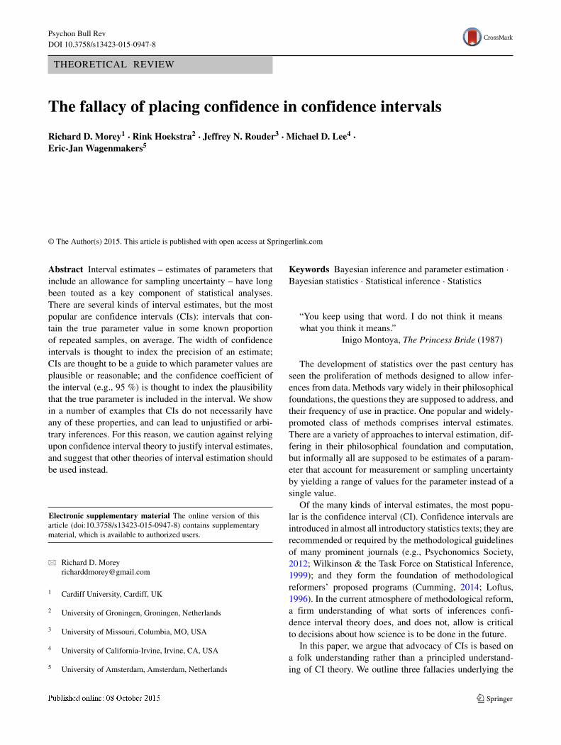
The fact that we can have 100 % certainty that a 50 % CIcontains the true value is a specific case of a more gen-eral problem flowing from the FCF. The shaded regions inFig. 2, left column, show when the true value is contained inthe various confidence procedures for all possible pairs ofobservations. The top, middle, and bottom row correspondto the sampling distribution, nonparametric/UMP, and theBayes procedures, respectively. Because each procedure isa 50 % confidence procedure, in each plot the shaded areaoccupies 50 % of the larger square delimiting the possibleobservations. The points ‘a’ and ‘b’ are the bubble patternsin Fig. 1a and b, respectively; point ‘b’ is in the shadedregion for each intervals because the true value is includedin every kind of interval, as shown in Fig. 1b; likewise, ‘a’is outside every shaded region because all CIs exclude thetrue value for this observed bubble pair.

Instead of considering the bubbles themselves, we mightalso translate their locations into the mean location y and thedifference between them, b = y2 − y1. We can do this with-out loss of any information: y contains the point estimate ofthe hatch location, and b contains the information about theprecision of that estimate. Figure 2, right column, shows thesame information as in the left column, except as a functionof y and b. The figures in the right column are 45◦ clock-wise rotations of those in the left. Although the two columnsshow the same information, the rotated right column revealsa critical fact: the various confidence procedures havedifferent probabilities of containing the true value when thedistance between the bubbles varies.

To see this, examine the horizontal line under point ‘a’ inFig. 2b. The horizontal line is the subset of all bubble pairsthat show the same difference between the bubbles as thosein Fig. 1a: 0.5 meters. About 31 % of this line falls under theshaded region, meaning that in the long run, 31 % of sam-pling distributions intervals will contain the true value, whenthe bubbles are 0.5 meters apart. For the nonparametric andUMP intervals (middle row), this percentage is only about5 %. For the Bayes interval (bottom row), it is exactly 50 %.

Believing the FCF implies believing that we can usethe long-run probability that a procedure contains the truevalue as an index of our post-data certainty that a partic-ular interval contains the true value. But in this case, wehave identified two long-run probabilities for each interval:the average long-run probability not taking into account theobserved difference — that is, 50 % — and the long-runprobability taking into account b which, for the samplingdistribution interval is 31 % and for the nonparametric/UMPintervals is 5 %. Both are valid long-run probabilities; whichdo we use for our inference? Under FCF, both are valid.Hence the FCF leads to contradiction.

The existence of multiple, contradictory long-run proba-bilities brings back into focus the confusion between whatwe know before the experiment with what we know afterthe experiment. For any of these confidence procedures, weknow before the experiment that 50 % of future CIs willcontain the true value. After observing the results, condi-tioning on a known property of the data — such as, in thiscase, the variance of the bubbles — can radically alter ourassessment of the probability.

The problem of contradictory inferences arising frommultiple applicable long-run probabilities is an example ofthe “reference class” problem (Venn, 1888; Reichenbach,1949), where a single observed event (e.g., a CI) canbe seen as part of several long-run sequences, each witha different long-run probability. Fisher noted that whenthere are identifiable subsets of the data that have differ-ent probabilities of containing the true value — such asthose subsets with a particular value of d, in our confi-dence interval example — those subsets are relevant tothe inference (Fisher, 1959). The existence of relevant sub-sets means that one can assign more than one probabilityto an interval. Relevant subsets are identifiable in manyconfidence procedures, including the common classical Stu-dent’s t interval, where wider CIs have a greater probabilityof containing the true value (Buehler, 1959; Buehler &Feddersen, 1963; Casella, 1992; Robinson, 1979). Thereare, as far as we know, only two general strategies for elim-inating the threat of contradiction from relevant subsets:Neyman’s strategy of avoiding any assignment of proba-bilities to particular intervals, and the Bayesian strategy ofalways conditioning on the observed data, to be discussedsubsequently.

Psychon Bull Rev

y1

y 2

θ − 5 θ θ + 5

θ − 5

θ

θ + 5A

a

b

y

y 2−

y 1

−10

−5

0

5

10

θ − 5 θ θ + 5

B

a

b

Sam

p. D

ist.

y1

y 2

θ − 5 θ θ + 5

θ − 5

θ

θ + 5C

a

b

y

y 2−

y 1

−10

−5

0

5

10

θ − 5 θ θ + 5

D

a

b

Non

para

./UM

P

y1

y 2

θ − 5 θ θ + 5

θ − 5

θ

θ + 5E

a

b

y

y 2−

y 1

−10

−5

0

5

10

θ − 5 θ θ + 5

F

a

b

Baye

s

Fig. 2 Left: Possible locations of the first (y1) and second (y2) bub-bles. Right: y2 − y1 plotted against the mean of y1 and y2. Shadedregions show the areas where the respective 50 % confidence inter-val contains the true value. The figures in the top row (a, b) showthe sampling distribution interval; the middle row (c, d) shows the NP

and UMP intervals; the bottom row (e, f) shows the Bayes interval.Points ‘a’ and ‘b’ represent the pairs of bubbles from Fig. 1a and b,respectively. An interactive version of this figure is available at http://learnbayes.org/redirects/CIshiny1.html

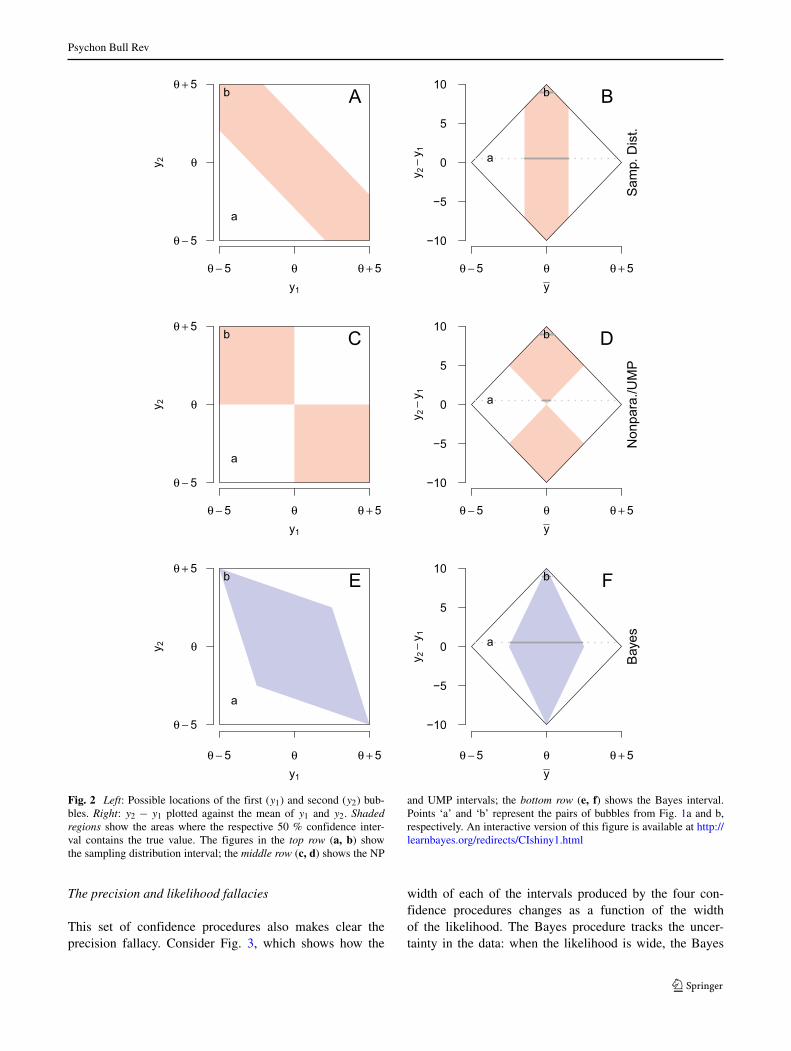
The precision and likelihood fallacies

This set of confidence procedures also makes clear theprecision fallacy. Consider Fig. 3, which shows how the

width of each of the intervals produced by the four con-fidence procedures changes as a function of the widthof the likelihood. The Bayes procedure tracks the uncer-tainty in the data: when the likelihood is wide, the Bayes

Psychon Bull Rev

0 2 4 6 8 10

0

2

4

6

8

10

Uncertainty (width of likelihood, meters)

CI w

idth

(met

ers)

NP

SD

UMP

B

Fig. 3 The relationship between CI width and the uncertainty in theestimation of the hatch location for the four confidence procedures.SD: Sampling distribution procedure; NP: Nonparametric procedure;UMP: UMP procedure; B: Bayes procedure. Note that the NP andUMP procedures overlap when the width of the likelihood is > 5. Aninteractive version of this figure is available at http://learnbayes.org/redirects/CIshiny1.html

CI is wide. The reason for this necessary correspondencebetween the likelihood and the Bayes interval will bediscussed later.

Intervals from the sampling distribution procedure, incontrast, have a fixed width, and so cannot reveal any infor-mation about the precision of the estimate. The samplingdistribution interval is of the commonly-seen CI form

x ± C × SE,

Like the CI for a normal population mean with known popu-lation variance, the standard error — defined as the standarddeviation of the sampling distribution of x — is known andfixed; here, it is approximately 2.04 (see the supplement fordetails). This indicates that the long-run standard error —and hence, confidence intervals based on the standard error— cannot always be used as a guide to the uncertainty weshould have in a parameter estimate.

Strangely, the nonparametric procedure generates inter-vals whose widths are inversely related to the uncertaintyin the parameter estimates. Even more strangely, intervalsfrom the UMP procedure initially increase in width with theuncertainty in the data, but when the width of the likeli-hood is greater than 5 meters, the width of the UMP intervalis inversely related to the uncertainty in the data, like thenonparametric interval. This can lead to bizarre situations.Consider observing the UMP 50 % interval [1, 1.5]. This isconsistent with two possible sets of observations: (1, 1.5),and (−3.5, 6). Both of these sets of bubbles will lead to thesame CI. Yet the second data set indicates high precision,and the first very low precision! The UMP and sampling dis-tribution procedures share the dubious distinction that theirCIs cannot be used to work backwards to the observations.

In spite of being the “most powerful” procedure, the UMPprocedure clearly throws away important information.

To see how the likelihood fallacy is manifest in thisexample, consider again Fig. 3. When the uncertainty ishigh, the likelihood is wide; yet the nonparametric and UMPintervals are extremely narrow, indicating both false preci-sion and excluding almost all likely values. Furthermore,the sampling distribution procedure and the nonparametricprocedure can contain impossible values.4

Evaluating the confidence procedures

The rescuers who have been offered the four intervals abovehave a choice to make: which confidence procedure tochoose? We have shown that several of the confidence pro-cedures have counter-intuitive properties, but thus far, wehave not made any firm commitments about which confi-dence procedures should be preferred to the others. For thesake of our rescue team, who have a decision to make aboutwhich interval to use, we now compare the four proceduresdirectly. We begin with the evaluation of the proceduresfrom the perspective of confidence interval theory, thenevaluate them according to Bayesian theory.

As previously mentioned, confidence interval theoryspecifies that better intervals will include false values lessoften. Figure 4 shows the probability that each of the pro-cedures include a value θ ′ at a specified distance fromthe hatch θ . All procedures are 50 % confidence proce-dures, and so they include the true value θ 50 % of thetime. Importantly, however, the procedures include particu-lar false values θ ′ �= θ at different rates. See the interactiveversions of Figs. 1 and 4 linked in the figure captions for ahands-on demonstration.

The trivial procedure (T; gray horizontal line) is obvi-ously a bad interval because it includes every false valuewith the same frequency as the true value. This is analo-gous to a hypothesis test with power equal to its Type I errorrate. The trivial procedure will be worse than any other pro-cedure, unless the procedure is specifically constructed tobe pathological. The UMP procedure (UMP), on the otherhand, is better than every other procedure for every value ofθ ′. This is due to the fact that it was created by inverting amost-powerful test.

4In order to construct a better interval, a frequentist would typicallytruncate the interval to only the possible values, as was done in gen-erating the UMP procedure from the nonparametric procedure (e.g.,Spanos, 2011). This is guaranteed to lead to a better procedure. Ourpoint here is that it is a mistake to naively assume that a procedure hasgood properties on the basis that it is a confidence procedure. However,see Velicer et al. (2008) for an example of CI proponents includingimpossible values in confidence intervals, and Fidler and Thompson(2001) for a defense of this practice.

Psychon Bull Rev

The ordering among the three remaining procedures canbe seen by comparing their curves. The sampling distri-bution procedure (SD) is always superior to the Bayesprocedure (B), but not to the nonparametric procedure(NP). The nonparametric procedure and the Bayes proce-dure curves overlap, so one is not preferred to the other.Welch (1939) remarked that the Bayes procedure is “not thebest way of constructing confidence limits” using preciselythe frequentist comparison shown in Fig. 4 with the UMPinterval.5

The frequentist comparison between the procedures isinstructive, because we have arrived at an ordering of theprocedures employing the criteria suggested by Neymanand used by the modern developers of new confidence pro-cedures: coverage and power. The UMP procedure is thebest, followed by the sampling distribution procedure. Thesampling distribution procedure is better than the Bayes pro-cedure. The nonparametric procedure is not preferred to anyinterval, but neither is it the worst.

We can also examine the procedures from a Bayesianperspective, which is primarily concerned with whether theinferences are reasonable in light of the data and whatwas known before the data were observed (Howson andUrbach, 2006). We have already seen that interpreting thenon-Bayesian procedures in this way leads to trouble, andthat the Bayesian procedure, unsurprisingly, has better prop-erties in this regard. We will show how the Bayesian intervalwas derived in order to provide insight into why it has goodproperties.

Consider the left column of Fig. 5, which shows Bayesianreasoning from prior and likelihood to posterior and so-called credible interval. The prior distribution in the toppanel shows that before observing the data, all the loca-tions in this region are equally probable. Upon observingthe bubbles shown in Fig. 1a — also shown in the top ofthe “likelihood” panel — the likelihood is a function that is1 for all possible locations for the hatch, and 0 otherwise.To combine our prior knowledge with the new informationfrom the two bubbles, we condition what we knew before onthe information in the data by multiplying by the likelihood— or, equivalently, excluding values we know to be impos-sible — which results in the posterior distribution in thebottom row. The central 50 % credible interval contains allvalues in the central 50 % of the area of the posterior, shownas the shaded region. The right column of Fig. 5 shows asimilar computation using an informative prior distributionthat does not assume that all locations are equally likely, as

5Several readers of a previous draft of this manuscript noted that fre-quentists use the likelihood as well, and so may prefer the Bayesianprocedure in this example. However, as Neyman (1977) points out, thelikelihood has no special status to a frequentist; what matters is thefrequentist properties of the procedure, not how it was constructed.

False alternative θ'

Prob

abilit

y C

I con

tain

s va

lue

0.0

0.1

0.2

0.3

0.4

0.5

θ − 7.5 θ − 5 θ − 2.5 θ θ + 7.5θ + 5θ + 2.5

T

NP

UMP

B

SD

Fig. 4 The probability that each confidence procedure includes falsevalues θ ′. T: Trivial procedure; SD: Sampling distribution procedureNP: Nonparametric procedure; UMP: UMP procedure; B: Bayes pro-cedure. The line for the sampling distribution procedure (dashed line)is between the lines for the Bayes procedure and the UMP procedure.An interactive version of this figure is available at http://learnbayes.org/redirects/CIshiny1.html

might occur if some other information about the location ofthe submersible were available.

It is now obvious why the Bayesian credible interval hasthe properties typically ascribed to confidence intervals. Thecredible interval can be interpreted as having a 50 % proba-bility of containing the true value, because the values withinit account for 50 % of the posterior probability. It revealsthe precision of our knowledge of the parameter, in light ofthe data and prior, through its relationship with the posteriorand likelihood.

Of the five procedures considered, intervals from theBayesian procedure are the only ones that can be said tohave 50 % probability of containing the true value, uponobserving the data. Importantly, the ability to interpret theinterval in this way arises from Bayesian theory and notfrom confidence interval theory. Also importantly, it wasnecessary to stipulate a prior to obtain the desired interval;the interval should be interpreted in light of the stipulatedprior. Of the other four intervals, none can be justified asproviding a “reasonable” inference or conclusion from thedata, because of their strange properties and that there isno possible prior distribution that could lead to these pro-cedures. In this light, it is clear why Neyman’s rejection of“conclusions” and “reasoning” from data naturally flowedfrom his theory: the theory, after all, does not support suchideas. It is also clear that if they care about making rea-sonable inferences from data, scientists might want want toreject confidence interval theory as a basis for evaluatingprocedures.

We can now review what we know concerning the fourprocedures. Only the Bayesian procedure — when its inter-vals are interpreted as credible intervals — allows theinterpretation that there is a 50 % probability that the hatch

Psychon Bull Rev

Prio

r

θ − 10 θ − 5 θ θ + 5 θ + 10

Like

lihoo

d

Location

Post

erio

r

θ − 10 θ − 5 θ θ + 5 θ + 10

θ − 10 θ − 5 θ θ + 5 θ + 10

Locationθ − 10 θ − 5 θ θ + 5 θ + 10

Fig. 5 Forming Bayesian credible intervals. Prior information (top)is combined with the likelihood information from the data (middle)to yield a posterior distribution (bottom). In the likelihood plots, theshaded regions show the locations within 5 meters of each bubble;the dark shaded regions show where these overlap, indicating the

possible location of the hatch θ . In the posterior plots, the central 50 %region (shaded region within posterior) shows one possible 50 % cred-ible interval, the central credible interval. An interactive version of thisfigure is available at http://learnbayes.org/redirects/CIshiny1.html

is located in the interval. Only the Bayesian procedure prop-erly tracks the precision of the estimate. Only the Bayesianprocedure covers the plausible values in the expected way:the other procedures produce intervals that are known withcertainty — by simple logic — to contain the true value, butstill are “50 %” intervals. The non-Bayesian intervals haveundesirable, even bizarre properties, which would lead anyreasonable analyst to reject them as a means to draw infer-ences. Yet the Bayesian procedure is judged by frequentistCI theory as inferior.

The disconnect between frequentist theory and Bayesiantheory arises from the different goals of the two theories.Frequentist theory is a “pre-data” theory. It looks forward,devising procedures that will have particular average prop-erties in repeated sampling (Jaynes, 2003; Mayo, 1981;1982) in the future (see also Neyman, 1937, p. 349). Thisthinking can be clearly seen in Neyman (1941) as quotedabove: reasoning ends once the procedure is derived. Con-fidence interval theory is vested in the average frequencyof including or excluding true and false parameter values,respectively. Any given inference may — or may not — bereasonable in light of the observed data, but this is not Ney-man’s concern; he disclaims any conclusions or beliefs onthe basis of data. Bayesian theory, on the other hand, is apost-data theory: a Bayesian analyst uses the information inthe data to determine what is reasonable to believe, in lightof the model assumptions and prior information.

Using an interval justified by a pre-data theory to makepost-data inferences can lead to unjustified, and possiblyarbitrary, inferences. This problem is not limited to the ped-agogical submersible example (Berger and Wolpert, 1988;Wagenmakers et al., 2014) though this simple example isinstructive for identifying these issues. In the next sectionwe show how a commonly-used confidence interval leads tosimilarly flawed post-data inferences.

Example 2: A confidence interval in the wild

The previous example was designed to show, in an accessi-ble example, the logic of confidence interval theory. Further,it showed that confidence procedures cannot be assumed tohave the properties that analysts desire.

When presenting the confidence intervals, CI proponentsalmost always focus on estimation of the mean of a normaldistribution. In this simple case, frequentist and Bayesian(with a “non-informative” prior) answers numerically coin-cide.6 However, the proponents of confidence intervalssuggest the use of confidence intervals for many otherquantities: for instance, standardized effect size Cohen’s

6This should not be taken to mean that inference by confidence inter-vals is not problematic even in this simple case; see e.g., Brown (1967)and Buehler & Feddersen (1963).

Psychon Bull Rev

d (Cumming and Finch, 2001), medians (Bonett & Price,2002; Olive, 2008), correlations (Zou, 2007), ordinal associ-ation (Woods, 2007), and many others. Quite often authorsof such articles provide no analysis of the properties ofthe proposed confidence procedures beyond showing thatthey contain the true value in the correct proportion ofsamples: that is, that they are confidence procedures. Some-times the authors provide an analysis of the frequentistproperties of the procedures, such as average width. Thedevelopers of new confidence procedures do not, as a rule,examine whether their procedures allow for valid post-datareasoning.

As the first example showed, a sole focus on frequen-tist properties of procedures is potentially disastrous forusers of these confidence procedures because a confidenceprocedure has no guarantee of supporting reasonable infer-ences about the parameter of interest. Casella (1992) under-scores this point with confidence intervals, saying that “wemust remember that practitioners are going to make con-ditional (post-data) inferences. Thus, we must be able toassure the user that any inference made, either pre-dataor post-data, possesses some definite measure of validity”(p. 10). Any development of an interval procedure thatdoes not, at least in part, focus on its post-data propertiesis incomplete at best and extremely misleading at worst:caveat emptor.

Can such misleading inferences occur using proceduressuggested by proponents of confidence intervals, and in useby researchers? The answer is yes, which we will show byexamining a confidence interval for ω2, the proportion ofvariance accounted for in ANOVA designs. The parame-ter ω2 serves as a measure of effect size when there aremore than two levels in a one-way design. This intervalwas suggested by Steiger (2004, see also Steiger & Fouladi,1997), cited approvingly by Cumming (2014), implementedin software for social scientists (e.g., Kelley, 2007a, b), andevaluated, solely for its frequentist properties, by Finch andFrench (2012). The problems we discuss here are shared byother related confidence intervals, such as confidence inter-vals for η2, partial η2, the noncentrality parameter of theF distribution, the signal-to-noise ratio f , RMSSE �, andothers discussed by Steiger (2004).

Steiger (2004) introduces confidence intervals by empha-sizing a desire to avoid significance tests, and to focus moreon the precision of estimates. Steiger says that “the scien-tist is more interested in knowing how large the differencebetween the two groups is (and how precisely it has beendetermined) than whether the difference between the groupsis 0” (pp. 164-165). Steiger and Fouladi (1997) say that“[t]he advantage of a confidence interval is that the widthof the interval provides a ready indication of the precisionof measurement...” (p. 231). Given our knowledge of theprecision fallacy these statements should raise a red flag.

Steiger then offers a confidence procedure for ω2 byinverting a significance test. Given the strange behavior ofthe UMP procedure in the submersible example, this tooshould raise a red flag. A confidence procedure based on atest — even a good, high-powered test — will not in generalyield a procedure that provides for reasonable inferences.We will outline the logic of building a confidence interval byinverting a significance test before showing how Steiger’sconfidence interval behaves with data.

To understand how a confidence interval can be built byinverting a significance test, consider that a two-sided sig-nificance test of size α can be thought of as a combination oftwo one-sided tests at size α/2: one for each tail. The two-sided test rejects when one of the one-tailed tests rejects. Tobuild a 68 % confidence interval (i.e., an interval that coversthe true value as often as the commonly-used standard errorfor the normal mean), we can use two one-sided tests of size(1− .68)/2 = .16. Suppose we have a one-way design withthree groups and N = 10 participants in each group. Theeffect size ω2 in such a design indexes how large F will be:larger ω2 values tend to yield larger F values. The distribu-tion of F given the effect size ω2 is called the noncentral Fdistribution. When ω2 = 0 — that is, there is no effect —the familiar central F distribution is obtained.

Consider first a one-sided test that rejects when F islarge. Figure 6a shows that a test of the null hypothesisthat ω2 = .1 would yield p = .16 when F(2, 27) = 5.If we tested larger values of ω2, the F value would notlead to a rejection; if we tested smaller values of ω2, theywould be rejected because their p values would be below.16. The gray dashed line in Fig. 6a shows the noncen-tral F(2, 27) distribution for ω2 = .2; it is apparent thatthe p value for this test would be greater than .16, andhence ω2 = .2 would not be rejected by the upper-tailedtest of size .16. Now consider the one-sided test that rejectswhen F is small. Figure 6b shows that a test of the nullhypothesis that ω2 = .36 would yield p = .16 whenF(2, 27) = 5; any ω2 value greater than .36 would berejected with p < .16, and any ω2 value less than .36would not.

Considering the two one-tailed tests together, for any ω2

value in [.1, .36], the p value for both one-sided tests willbe greater than p > .16 and hence will not lead to a rejec-tion. A 68 % confidence interval for when F(2, 27) = 5 canbe defined as all ω2 values that are not rejected by either ofthe two-tailed tests, and so [.1, .36] is taken as a 68 % con-fidence interval. A complication arises, however, when thep value from the ANOVA F test is greater than α/2; by def-inition, the p value is computed under the hypothesis thatthere is no effect, that is ω2 = 0. Values of ω2 cannot be anylower than 0, and hence there are no ω2 values that would berejected by the upper tailed test. In this case the lower boundon the CI does not exist. A second complication arises when

Psychon Bull Rev

0 5 10 15F statistic

Den

sity

ω2=0.1

42%

16%

ω2=0.2

A

0 5 10 15F statistic

Den

sity

ω2=0.3658%

16%

ω2=0.2

B

Fig. 6 Building a confidence interval by inverting a significance test.A: Two noncentral F distributions, with true ω2 = .1 (blue solid line)and true ω2 = .2 (dashed gray line). When F(2, 27) = 5, the upper-tailed p value for these tests are .16 and .42, respectively. B: Twononcentral F distributions, with true ω2 = .36 (red solid line) and trueω2 = .2 (dashed gray line). When F(2, 27) = 5, the lower-tailed p

value for these tests are .16 and .58, respectively

the p value is greater than 1−α/2: all lower-tailed tests willreject, and hence the upper bound of the CI does not exist. Ifa bound does not exist, Steiger (2004) arbitrarily sets it at 0.

To see how this CI works in practice, suppose we design athree-group, between-subjects experiment withN = 10 par-ticipants in each group and obtain an F(2, 27) = 0.18, p =0.84. Following recommendations for good analysis prac-tices (e.g., Psychonomics society 2012; Wilkinson & theTask Force on Statistical Inference, 1999, we would like tocompute a confidence interval on the standardized effectssize ω2. Using software to compute Steiger’s CI, we obtainthe 68 % confidence interval [0, 0.01].

Figure 7a (top interval) shows the resulting 68 % interval.If we were not aware of the fallacies of confidence intervals,we might publish this confidence interval thinking it pro-vides a good measure of the precision of the estimate of ω2.Note that the lower limit of the confidence interval is exactly0, because the lower bound did not exist. In discussing thissituation Steiger and Fouladi (1997) say

“[Arbitrarily setting the confidence limit at 0] main-tains the correct coverage probability for the confi-dence interval, but the width of the confidence interval

may be suspect as an index of the precision of mea-surement when either or both ends of the confidenceinterval are at 0. In such cases, one might considerobtaining alternative indications of precision of mea-surement, such as an estimate of the standard error ofthe statistic.” (Steiger and Fouladi, 1997, p. 255)

Steiger (2004) further notes that “relationship [betweenCI width and precision] is less than perfect and is seri-ously compromised in some situations for several reasons”(p. 177). This is a rather startling admission: a major partof the justification for confidence intervals, including theone computed here, is that confidence intervals supposedlyallow an assessment of the precision with which the param-eter is estimated. The confidence interval fails to meet thepurpose for which it was advocated in the first place, butSteiger does not indicate why, nor under what conditions theCI will successfully track precision.

We can confirm the need for Steiger’s caution — essen-tially, a warning about the precision fallacy — by lookingat the likelihood, which is the probability density of theobserved F statistic computed for all possible true values ofω2. Notice how narrow the confidence interval is comparedto the likelihood of ω2. The likelihood falls much moreslowly as ω2 gets larger than the confidence interval wouldappear to imply, if we believed the precision fallacy. We canalso compare the confidence interval to a 68 % Bayesiancredible interval, computed assuming standard “noninfor-mative” priors on the means and the error variance.7 TheBayesian credible interval is substantially wider, revealingthe imprecision with which ω2 is estimated.

Figure 7b shows the same case, but for a slightly smallerF value. The precision with which ω2 is estimated has notchanged to any substantial degree; yet now the confidenceinterval contains only the value ω2 = 0: or, more accurately,the confidence interval is empty because this F value wouldalways be rejected by one of the pairs of one-sided tests thatled to the construction of the confidence interval. As Steigerpoints out, a “zero-width confidence interval obviously doesnot imply that effect size was determined with perfect pre-cision,” (p. 177), nor can it imply that there is a 68 %probability that ω2 is exactly 0. This can be clearly seen byexamining the likelihood and Bayesian credible interval.

Some authors (e.g., Dufour, 1997) interpret empty confi-dence intervals as indicative of model misfit. In the case ofthis one sample design, if the confidence interval is emptythen the means are more similar than would be expected

7See the supplement for details. We do not generally advocate non-informative priors on parameters of interest (Rouder et al., 2012;Wetzels et al., 2012); in this instance we use them as a comparisonbecause many people believe, incorrectly, that confidence intervalsnumerically correspond to Bayesian credible intervals with noninfor-mative priors.

Psychon Bull Rev

0.0 0.2 0.4ω2

F = 0.175Conf. = 0.68

A

Like

lihoo

d

0.0 0.2 0.4ω2

F = 0.174Conf. = 0.68

B

0.0 0.2 0.4ω2

F = 0.174Conf. = 0.7

C

Like

lihoo

d

0.0 0.4 0.8ω2

F = 4.237Conf. = 0.95

D

Fig. 7 Likelihoods, confidence intervals, and Bayesian credible inter-vals (highest posterior density, or HPD, intervals) for four hypotheticalexperimental results. In each figure, the top interval is Steiger’s (2004)confidence interval for ω2; the bottom interval is the Bayesian HPD.See text for details

even under the null hypothesis α/2 of the time; that is,p > 1 − α/2, and hence F is small. If this model rejectionsignificance test logic is used, the confidence interval itselfbecomes uninterpretable as the model gets close to rejec-tion, because it appears to indicate false precision (Gelman,2011). Moreover, in this case the p value is certainly moreinformative than the CI; the p value provides graded infor-mation that does not depend on the arbitrary choice of α,while the CI is simply empty for all values of p > 1− α/2.

Panel C shows what happens when we increase the confi-dence coefficient slightly to 70 %. Again, the precision withwhich the parameter is estimated has not changed, yet theconfidence interval now again has nonzero width.

Figure 7d shows the results of an analysis withF(2, 27) = 4.24, p = 0.03, and using a 95 % confidenceinterval. Steiger’s interval has now encompassed most of thelikelihood, but the lower bound is still “stuck” at 0. In thissituation, Steiger and Fouladi advise us that the width of theCI is “suspect” as an indication of precision, and that weshould “obtain[] [an] alternative indication[] of precision ofmeasurement.” As it turns out, here the confidence intervalis not too different from the credible interval, though theconfidence interval is longer and is unbalanced. However,we would not know this if we did not examine the likeli-hood and the Bayesian credible interval; the only reason weknow the confidence interval has a reasonable width in this

particular case is its agreement with the actual measures ofprecision offered by the likelihood and the credible interval.

How often will Steiger’s confidence procedure yield a“suspect” confidence interval? This will occur wheneverthe p value for the corresponding F test is p > α/2;for a 95 % confidence interval, this means that wheneverp > 0.025, Steiger and Fouladi recommend against usingthe confidence interval for precisely the purpose that they—and other proponents of confidence intervals — recommendit for. This is not a mere theoretical issue; moderately-sized p values often occur. In a cursory review ofpapers citing Steiger (2004), we found many that obtainedand reported, without note, suspect confidence intervalsbounded at 0 (e.g., Cumming, Sherar, Gammon, Standage,& Malina, 2012; Gilroy & Pearce 2014; Hamerman& Morewedge,2015; Lahiri, Maloney, Rogers, & Ge, 2013;Hamerman & Morewedge, 2015; Todd, Vurbic, & Bouton,2014; Winter et al., 2014). The others did not use confi-dence intervals, instead relying on point estimates of effectsize and p values (e.g., Hollingdale & Greitemeyer, 2014);but from the p values it could be inferred that if they hadfollowed “good practice” and computed such confidenceintervals, they would have obtained intervals that accord-ing to Steiger could not be interpreted as anything but aninverted F test.

It makes sense, however, that authors using confidenceintervals would not note that the interpretation of their con-fidence intervals is problematic. If confidence intervals trulycontained the most likely values, or if they were indices ofthe precision, or if the confidence coefficient indexed theuncertainty we should have that the parameter is in an inter-val, then it would seem that a CI is a CI: what you learn fromone is the same as what you learn from another. The ideathat the p value can determine whether the interpretation ofa confidence interval is possible is not intuitive in light ofthe way CIs are typically presented.

We see no reason why our ability to interpret an inter-val should be compromised simply because we obtained ap value that was not low enough. Certainly, the confidencecoefficient is arbitrary; if the width is suspect for one con-fidence coefficient, it makes little sense that the CI widthwould become acceptable just because we changed the con-fidence coefficient so the interval bounds did not include0. Also, if the width is too narrow with moderate p val-ues, such that it is not an index of precision, it seems thatthe interval will be too wide in other circumstances, possi-bly threatening the interpretation as well. This was evidentwith the UMP procedure in the submersible example: theUMP interval was too narrow when the data provided lit-tle information, and was too wide when the data providedsubstantial information.

Steiger and Fouladi (1997) summarize the central prob-lem with confidence intervals when they say that in order

Psychon Bull Rev

to maintain the correct coverage probability — a frequentistpre-data concern — they sacrifice the very thing researcherswant confidence intervals to be: a post-data index of theprecision of measurement. If our goal is to move awayfrom significance testing, we should not use methods whichcannot be interpreted except as inversions of significancetests. We agree with Steiger and Fouladi that researchersshould consider obtaining alternative indications of preci-sion of measurement; luckily, Bayesian credible intervalsfit the bill rather nicely, rendering confidence intervalsunnecessary.

Discussion

Using the theory of confidence intervals and the supportof two examples, we have shown that CIs do not have theproperties that are often claimed on their behalf. Confidenceinterval theory was developed to solve a very constrainedproblem: how can one construct a procedure that producesintervals containing the true parameter a fixed proportionof the time? Claims that confidence intervals yield anindex of precision, that the values within them are plau-sible, and that the confidence coefficient can be read asa measure of certainty that the interval contains the truevalue, are all fallacies and unjustified by confidence intervaltheory.

Good intentions underlie the advocacy of confidenceintervals: it would be desirable to have procedures with theproperties claimed. The FCF is driven by a desire to assessthe plausibility that an interval contains the true value; thelikelihood fallacy is driven by a desire to determine whichvalues of the parameter should be taken seriously; and theprecision fallacy is driven by a desire to quantify the preci-sion of the estimates. We support these goals (Morey et al.,2014), but confidence interval theory is not the way toachieve them.

Guidelines for interpreting and reporting intervals

Frequentist theory can be counter-intuitive at times; asFisher was fond of pointing out, frequentist theorists oftenseemed disconnected with the concerns of scientists, devel-oping methods that did not suit their needs (e.g., Fisher,1955, p. 70). This has lead to confusion where practi-tioners assume that methods designed for one purposewere really meant for another. In order to help miti-gate such confusion, here we would like to offer read-ers a clear guide to interpreting and reporting confidenceintervals.

Once one has collected data and computed a confidenceinterval, how does one then interpret the interval? Theanswer is quite straightforward: one does not – at least not

within confidence interval theory.8 As Neyman and otherspointed out repeatedly, and as we have shown, confidencelimits cannot be interpreted as anything besides the result ofa procedure that will contain the true value in a fixed pro-portion of samples. Unless an interpretation of the intervalcan be specifically justified by some other theory of infer-ence, confidence intervals must remain uninterpreted, lestone make arbitrary inferences or inferences that are contra-dicted by the data. This applies even to “good” confidenceintervals, as these are often built by inverting significancetests and may have strange properties (e.g., Steiger, 2004).

In order to help mitigate confusion in the scientific liter-ature, we suggest the following guidelines for reporting ofintervals informed by our discussion in this manuscript.

Report credible intervals instead of confidence inter-vals We believe any author who chooses to use confidenceintervals should ensure that the intervals correspond numer-ically with credible intervals under some reasonable prior.Many confidence intervals cannot be so interpreted, but ifthe authors know they can be, they should be called “credi-ble intervals”. This signals to readers that they can interpretthe interval as they have been (incorrectly) told they caninterpret confidence intervals. Of course, the correspondingprior must also be reported. This is not to say that one can-not also refer to credible intervals as confidence intervals,if indeed they are; however, readers are likely more inter-ested in knowing that the procedure allows valid post-datainference — not pre-data inference — if they are inter-ested arriving at substantive conclusions from the computedinterval.

Do not use confidence procedures whose Bayesian prop-erties are not known As Casella (1992) pointed out, thepost-data properties of a procedure are necessary for under-standing what can be inferred from an interval. Any proce-dure whose Bayesian properties have not been explored mayhave properties that make it unsuitable for post-data infer-ence. Procedures whose properties have not been adequatelystudied are inappropriate for general use.

Warn readers if the confidence procedure does not cor-respond to a Bayesian procedure If it is known that aconfidence interval does not correspond to a Bayesian pro-cedure, warn readers that the confidence interval cannot be

8Some recent writers have suggested the replacement of Neyman’sbehavioral view on confidence intervals with a frequentist viewfocused on tests at various levels of “stringency” (see, e.g., Mayo &Cox, 2006; Mayo & Spanos, 2006). Readers who prefer a frequentistparadigm may wish to explore this approach; however, we are unawareof any comprehensive account of CIs within this paradigm, and regard-less, it does not offer the properties desired by CI proponents. This isnot to be read as an argument against it, but rather a warning that onemust make a choice.

Psychon Bull Rev

interpreted as having an X% probability of containing theparameter, that cannot be interpreted in terms of the preci-sion of measurement, and that cannot be said to contain thevalues that should be taken seriously: the interval is merelyan interval that, prior to sampling, had an X% probabilityof containing the true value. Authors choosing to report CIshave a responsibility to keep their readers from invalid infer-ences, because it is almost certain that without a warningreaders will misinterpret them (Hoekstra et al., 2014).

Never report a confidence interval without noting theprocedure and the corresponding statistics As we havedescribed, there are many different ways to construct con-fidence intervals, and they will have different properties.Some will have better frequentist properties than others;some will correspond to credible intervals, and others willnot. It is unfortunately common for authors to report con-fidence intervals without noting how they were constructedor even citing a source. As can be seen from the exam-ples we have presented, this is a terrible practice: withoutknowing which confidence procedure was used, it is unclearwhat can be inferred. In the submersible example, considera 50 % confidence interval .5 meters wide. This could cor-respond to very precise information (Bayesian interval) orvery imprecise information (UMP and nonparametric inter-val). Not knowing which procedure was used could lead toabsurd inferences. In addition, enough information shouldbe presented so that any reader can compute a different con-fidence interval or credible interval. In many cases, this iscovered by standard reporting practices, but in other casesmore information may need to be given.

Consider reporting likelihoods or posteriors instead Aninterval provides fairly impoverished information. Just asproponents of confidence intervals argue that CIs pro-vide more information than a significance test (althoughthis is debatable for many CIs), a likelihood or a pos-terior provides much more information than an interval.Recently, Cumming (2014) has proposed so-called “cat’seye” intervals which correspond to Bayesian posteriorsunder a “non-informative” prior for normally distributeddata. With modern scientific graphics so easy to create,we see no reason why likelihoods and posteriors cannotaugment or even replace intervals in most circumstances(e.g., Kruschke, 2010). With a likelihood or a posterior, thearbitrariness of the confidence or credibility coefficient isavoided altogether.

A complete account of Bayesian statistics is beyond thescope of this paper (and indeed, can fill entire courses).In recent years, a number of good resources have beendeveloped for readers wishing to learn more about appliedBayesian statistics, including estimation of posterior distri-butions and credible intervals: on the less technical side,

there are texts by Bolstad (2007), Lee and Wagenmakers(2013), and Lynch (2007); on the more technical side aretexts by Jackman (2009), Ntzoufras (2009), and Gelmanet al. (2004). There are also numerous resources on theworld wide web to help beginners. For readers wishing to trysome simple examples, the supplement to this article con-tains R code to estimate posterior distributions and credibleintervals for the examples in this paper.

Confidence intervals versus credible intervals

One of the misconceptions regarding the relationshipbetween Bayesian inference and frequentist inference is thatthey will lead to the same inferences, and hence all con-fidence intervals can simply be interpreted in a Bayesianway. In the case where data are normally distributed, forinstance, there is a particular prior that will lead to a con-fidence interval that is numerically identical to Bayesiancredible intervals computed using the Bayesian posterior(Jeffreys, 1961; Lindley, 1965). This might lead one to sus-pect that it does not matter whether one uses confidenceprocedures or Bayesian procedures. We showed, however,that confidence intervals and credible intervals can disagreemarkedly. The only way to know that a confidence inter-val is numerically identical to some credible interval is toprove it. The correspondence cannot — and should not —be assumed.

More broadly, the defense of confidence procedures bynoting that, in some restricted cases, they numerically cor-respond to Bayesian procedures is actually no defense atall. One must first choose which confidence procedure, ofmany, to use; if one is committed to the procedure thatallows a Bayesian interpretation, then one’s time is muchbetter spent simply applying Bayesian theory. If the bene-fits of Bayesian theory are desired — and they clearly are,by proponents of confidence intervals — then there is noreason why Bayesian inference should not be applied in itsfull generality, rather than using the occasional correspon-dence with credible intervals as a hand-waving defense ofconfidence intervals.

It is important to emphasize, however, that for many ofthe confidence procedures presented in the applied statis-tical literature, no effort has been made to show that theintervals have the properties that proponents of confidenceintervals desire. We should expect, as a matter of course,that developers of new confidence intervals show that theirintervals have the desired inferential properties, instead ofjust nominal coverage of the true value and “short” width.Because developers of confidence intervals have not donethis, the push for confidence intervals rests on uncertainground. Adopting Bayesian inference, where all inferencesarise within a logical, unified framework, would render theproblems of assessing the properties of these confidence

Psychon Bull Rev

procedures moot. If desired, coverage of a Bayesian proce-dure can also be assessed; but if one is interested primarilyin reasonable post-data inference, then Bayesian propertiesshould be the priority, not frequentist coverage (cf. Gelman,2008; Wasserman, 2008).

For advocates of reasoning by intervals, adoptingBayesian inference would have other benefits. The end-points of a confidence interval are always set by the data.Suppose, however, we are interested in determining theplausibility that a parameter is in a particular range; forinstance, in the United States, it is against the law to executecriminals who are intellectually disabled. The criterion usedfor intellectual disability in the US state of Florida is havinga true IQ less than 70. Since IQ is measured with error, onemight ask what confidence we have that a particular crimi-nal’s true IQ is less than 70 (see Anastasi and Urbina (1997),or Cronbach (1990), for an overview of confidence intervalsfor IQ). In this case, the interval we would like to assess forplausibility is no longer a function of the sample. The long-run probability that the true value is inside a fixed intervalis unknown and is either 0 or 1, and hence no confidenceprocedure can be constructed, even though such informationmay be critically important to a researcher, policy maker, orcriminal defendant (Pratt et al., 1995).

Even in seemingly simple cases where a fixed inter-val is nested inside a CI, or vice versa, one cannot drawconclusions about the plausibility of a fixed interval. Onemight assume that an interval nested within a CI must havelower confidence than the CI, given that it is shorter; how-ever, as shown in Fig. 1b, a 100 % confidence interval (thelikelihood) is nested within some of the 50 % confidenceintervals. Likewise, one might believe that if a CI is nestedwithin a fixed interval, then the fixed interval must havegreater probability than the interval. But in Fig. 1a, one canimagine a fixed interval just larger than the 50 % UMPinterval; this will have much lower than 50 % probabilityof containing the true value, due to the fact that it occupiesa small proportion of the likelihood. Knowledge that theFCF is a fallacy prohibits one from using confidence inter-vals to assess the probability of fixed intervals. Bayesianprocedures, on the other hand, offer the ability to computethe plausibility of any given range of values. Because allsuch inferences must be made from the posterior distribu-tion, inferences must remain mutually consistent (Lindley,1985; see also Fisher, 1935, for a similar argument).

Moving to credible intervals from confidence intervalswould necessitate a shift in thinking, however, away froma test-centric view with respect to intervals (e.g., “is 0in the interval?”). Although every confidence interval canbe interpreted as a test, credible intervals cannot be sointerpreted. Assessing the Bayesian credibility of a spe-cific parameter value by checking whether it is includedin a credible interval is, as Berger (2006) puts it, “simply

wrong.” When testing a specific value is of interest (such asa null hypothesis), that specific value must be assigned non-zero probability a priori. While not conceptually difficult, itis beyond the scope of this paper; see Rouder et al. (2009),Wagenmakers et al. (2008), or Dienes (2011) for accessibleaccounts.

Finally, we believe that in science, the meaning of ourinferences are important. Bayesian credible intervals sup-port an interpretation of probability in terms of plausibility,thanks to the explicit use of a prior. Confidence intervals, onthe other hand, are based on a philosophy that does not allowinferences about plausibility, and does not utilize prior infor-mation. Using confidence intervals as if they were credibleintervals is an attempt to smuggle Bayesian meaning intofrequentist statistics, without proper consideration of a prior.As they say, there is no such thing as a free lunch; one mustchoose.We suspect that researchers, given the choice, wouldrather specify priors and get the benefits that come fromBayesian theory. We should not pretend, however, that thechoice need not be made. Confidence interval theory andBayesian theory are not interchangeable, and should not betreated as so.

Conclusion

We have suggested that confidence intervals do not supportthe inferences that their advocates believe they do. It is aninteresting question how the theory of confidence intervalsbegan with Neyman as a method of avoiding the problemof reasoning from data by making dichotomous statements(Neyman 1937, 1941), eventually becoming a method thatmany believe is the best way to reason from data (e.g.Cumming & Finch, 2005; Cumming & Fidler, 2009) and away to avoid dichotomous statements (e.g. Cumming, 2014;Hoekstra, Finch, Kiers, & Johnson, 2006; Wilkinson & theTask Force on Statistical Inference, 1999). Regardless ofhow this confusion started, we believe it should be recog-nized that confidence interval theory offers only the shal-lowest of interpretations, and is not well-suited to the needsof scientists.

We do not believe that the theory of confidence intervalsprovides a viable foundation for the future of psychologicalmethods. Confidence procedures that do not have Bayesianproperties have other undesirable properties; confidenceprocedures that do have Bayesian properties can be justi-fied using Bayesian theory. If we were to give up the useof confidence procedures, what would we lose? Abandon-ing the use of confidence procedures means abandoning amethod that merely allows us to create intervals that includethe true value with a fixed long-run probability. We sus-pect that if researchers understand that this is the only thingthey will be losing, they will not consider it a great loss. Byadopting Bayesian inference, they will gain a way of making

Psychon Bull Rev

principled statements about precision and plausibility. Ulti-mately, this is exactly what the advocates of CIs havewanted all along.

Open Access This article is distributed under the terms ofthe Creative Commons Attribution 4.0 International License(http://creativecommons.org/licenses/by/4.0/), which permits unre-stricted use, distribution, and reproduction in any medium, providedyou give appropriate credit to the original author(s) and the source,provide a link to the Creative Commons license, and indicate ifchanges were made.

Author Note We thank Mijke Rhemtulla for helpful discussion dur-ing the drafting of the manuscript, and many online commenters fortheir helpful comments, both positive and negative. Supplementarymaterial, all code, and the source for this document are availableat https://github.com/richarddmorey/ConfidenceIntervalsFallacy. Thiswork was partially funded by the European Research Council grant“Bayes or Bust” awarded to Eric-Jan Wagenmakers, and by NationalScience Foundation grants BCS-1240359 and SES-102408 awarded toJeffrey N. Rouder.

References

Anastasi, A., & Urbina, S. (1997). Psychological testing, 7th ed.London: Prentice-Hall International.

Basu, D. (1981). On ancillary statistics, pivotal quantities, and con-fidence statements. In Chaubey, Y.P., & Dwivedi, T.D. (Eds.),Topics in applied statistics (pp. 1–29). Montreal: Concordia Uni-versity.

Berger, J. O. (2006). Bayes factors. In Kotz, S., Balakrishnan, N.,Read, C., Vidakovic, B., & Johnson, N.L. (Eds.), Encyclopediaof statistical sciences (Second edition), (Vol. 1 pp. 378–386).Hoboken, New Jersey: John Wiley & Sons.

Berger, J. O., & Wolpert, R. L. (1988). The likelihood principle (2nded.) Hayward. CA: Institute of Mathematical Statistics.

Blaker, H., & Spjøtvoll, E. (2000). Paradoxes and improvements ininterval estimation. The American Statistician, 54(4), 242–247.

Bolstad, W. (2007). Introduction to Bayesian statistics. Hoboken:Wiley.

Bonett, D. G., & Price, R.M. (2002). Statistical inference for a lin-ear function of medians: Confidence intervals, hypothesis test-ing, and sample size requirements. Psychological Methods, 7,370–383.

Brown, L. (1967). The conditional level of Student’s t test. The Annalsof Mathematical Statistics, 38(4), 1068–1071.

Buehler, R. J. (1959). Some validity criteria for statisticalinferences. The Annals of Mathematical Statistics, 30(4), 845–863.

Buehler, R. J., & Feddersen, A. P. (1963). Note on a conditional prop-erty of Student’s t1. The Annals of Mathematical Statistics, 34(3),1098–1100.

Casella, G. (1992). Conditional inference from confidence sets. Lec-ture Notes-Monograph Series, 17, 1–12.

Casella, G., & Berger, R. L. (2002). Statistical inference. PacificGrove, CA, Duxbury.

Cronbach, L. J. (1990). Essentials of psychological testing, 5th ed.New York: Harper & Row.

Cumming, G. (2014). The new statistics: Why and how. PsychologicalScience, 25, 7–29.

Cumming, G., & Fidler, F. (2009). Confidence intervals: Betteranswers to better questions. Zeitschrift fur Psychologie, 217,15–26.

Cumming, G., & Finch, S. (2001). A primer on the understanding,use, and calculation of confidence intervals that are based on cen-tral and noncentral distributions. Educational and PsychologicalMeasurement, 61, 532–574.

Cumming, G., & Finch, S. (2005). Inference by eye: Confidence inter-vals and how to read pictures of data. American Psychologist,60(2), 170–180.

Cumming, S. P., Sherar, L. B., Gammon, C., Standage, M., & Malina,R.M. (2012). Physical activity and physical self-concept in ado-lescence: A comparison of girls at the extremes of the biologi-cal maturation continuum. Journal of Research on Adolescence,22(4), 746–757.

Dienes, Z. (2011). Bayesian versus orthodox statistics: Which side areyou on? Perspectives on Psychological Science, 6, 274–290.

Dufour, J.-M. (1997). Some impossibility theorems in econometricswith applications to structural and dynamic models. Economet-rica, 65(6), 1365–1387.

Fidler, F., & Loftus, G. R. (2009). Why figures with errorbars should replace p values: Some conceptual argumentsand empirical demonstrations. Zeitschrift fur Psychologie, 217(1), 27–37.

Fidler, F., & Thompson, B. (2001). Computing correct confidenceintervals for ANOVA fixed- and random-effects effect sizes. Edu-cational and Psychological Measurement, 61, 575–604.

Finch, W.H., & French, B. F. (2012). A comparison of methodsfor estimating confidence intervals for omega-squared effect size.Educational and Psychological Measurement, 72(1), 68–77.

Fisher, R. A. (1935). The fiducial argument in statistical inference.Annals of eugenics, 6, 391–398.

Fisher, R. A. (1955). Statistical methods and scientific induction. Jour-nal of the Royal Statistical Society. Series B (Methodological), 17,69–78.

Fisher, R. A. (1959). Statistical methods and scientific inference (Sec-ond). Edinburgh: Oliver and Boyd.

Gelman, A. (2008). Rejoinder. Bayesian analysis, 3, 467–478.Gelman, A. (2011). Why it doesn’t make sense in general to

form confidence intervals by inverting hypothesis tests. [blogpost]. Retrieved from http://andrewgelman.com/2011/08/25/whyit doesnt m/

Gelman, A., Carlin, J. B., Stern, H. S., & Rubin, D. B. (2004). Bayesiandata analysis, 2nd edition. London: Chapman and Hall.

Gilroy, K. E., & Pearce, J.M. (2014). The role of local, distal, andglobal information in latent spatial learning. Journal of Experi-mental Psychology, 40(2), 212–224.

Hamerman, E. J., & Morewedge, C. K. (2015). Reliance on luck:Identifying which achievement goals elicit superstitious behav-ior. Personality and Social Psychology Bulletin, 41(3), 323–335.WOS:000349626400002.

Hoekstra, R., Finch, S., Kiers, H. A. L., & Johnson, A. (2006). Prob-ability as certainty: Dichotomous thinking and the misuse of pvalues. Psychonomic Bulletin & Review, 13, 1033–1037.

Hoekstra, R., Morey, R. D., Rouder, J. N., & Wagenmakers, E.-J.(2014). Robust misinterpretation of confidence intervals. Psycho-nomic Bulletin & Review, 21(5), 1157–1164.

Hollingdale, J., & Greitemeyer, T. (2014). The effect of online violentvideo games on levels of aggression. PLoS ONE, 9(11), e111–790.Retrieved from. doi:10.1371/journal.pone.0111790

Howson, C., & Urbach, P. (2006). Scientific reasoning: The Bayesianapproach. Illinois: Open Court: La Salle.

Jackman, S. (2009). Bayesian analysis for the social sciences. UnitedKingdom: Wiley.

Psychon Bull Rev

Jaynes, E. (2003). Probability theory: The logic of science. Cambridge:Cambridge University Press.

Jeffreys, H. (1961). Theory of probability, 3rd edition. New York:Oxford University Press.

Kelley, K. (2007a). Confidence intervals for standardized effect sizes:Theory, application, and implementation. Journal of StatisticalSoftware, 20(8).

Kelley, K. (2007b). Methods for the behavioral, educational, and socialsciences: An R package. Behavioral Research Methods, 39(4),979–984.

Kruschke, J. K. (2010). What to believe: Bayesian methods for dataanalysis. Trends in Cognitive Sciences, 14(7), 293–300.

Lahiri, D. K., Maloney, B., Rogers, J. T., & Ge, Y.-W. (2013). PuF,an antimetastatic and developmental signaling protein, interactswith the Alzheimer’s amyloid-beta precursor protein via a tissue-specific proximal regulatory element (PRE). Bmc Genomics, 14,68.

Lee, M.D., & Wagenmakers, E.-J. (2013). Bayesian cognitive model-ing: A practical course: Cambridge University Press.

Lehmann, E. H. (1959). Testing statistical hypotheses. New York:Wiley.

Lindley, D.V. (1965). Introduction to probability and statistics from aBayesian point of view, part 2: Inference. Cambridge: CambridgeUniversity Press.

Lindley, D.V. (1985). Making decisions, 2nd ed. London: Wiley.Loftus, G. R. (1993). A picture is worth a thousand p-values: On

the irrelevance of hypothesis testing in the computer age. Behav-ior Research Methods. Instrumentation and Computers, 25, 250–256.

Loftus, G. R. (1996). Psychology will be a much better science whenwe change the way we analyze data. Current directions in psycho-logical science, 5, 161–171.

Lynch, S.M. (2007). Introduction to applied Bayesian statistics andestimation for social scientists. New York: Springer.

Masson, M. E. J., & Loftus, G. R. (2003). Using confidence intervalsfor graphically based data interpretation. Canadian Journal ofExperimental Psychology, 57, 203–220.

Mayo, D.G. (1981). In defense of the Neyman-Pearson the-ory of confidence intervals. Philosophy of Science, 48(2), 269–280.

Mayo, D.G. (1982). On after-trial criticisms of Neyman-Pearson the-ory of statistics. PSA: Proceedings of the Biennial Meeting of thePhilosophy of Science Association, 1982.

Mayo, D.G., & Cox, D. R. (2006). Frequentist statistics as a theoryof inductive inference. Institute of Mathematical Statistics LectureNotes - Monograph Series, 49, 77–97.

Mayo, D.G., & Spanos, A. (2006). Severe testing as a basic conceptin a Neyman-Pearson philosophy of induction. British Journal forthe philosophy of science, 57, 323–357.

McGrayne, S. B. (2011). The theory that would not die. New Haven:Yale University Press.

Morey, R. D., Rouder, J. N., Verhagen, J., & Wagenmakers, E.-J.(2014). Why hypothesis tests are essential for psychological sci-ence: A comment on Cumming. Psychological Science, 1289–1290.

Neyman, J. (1934). On the two different aspects of the representativemethod: The method of stratified sampling and the method of pur-posive selection. Journal of the Royal Statistical Society, 97(4),558–625.

Neyman, J. (1937). Outline of a theory of statistical estimation basedon the classical theory of probability. Philosophical Transactionsof the Royal Society of London. Series A. Mathematical andPhysical Sciences, 236, 333-380.

Neyman, J. (1941). Fiducial argument and the theory of confidenceintervals. Biometrika, 32(2), 128–150.

Neyman, J. (1952). Lectures and conferences on mathematical statis-tics and probability. Washington, D.C.: Graduate School, U.S.Department of Agriculture.

Neyman, J. (1977). Frequentist probability and frequentist statistics.Synthese, 36(1), 97–131.

Ntzoufras, I. (2009). Bayesian modeling using WinBUGS. New Jersey:Wiley.

Olive, D. J. (2008). Applied robust statistics. online electronic book.Retrieved from, http://lagrange.math.siu.edu/Olive/ol-bookp.htm

Pratt, J.W. (1961). Book review: Testing Statistical Hypotheses, byE. L. Lehmann. Journal of the American Statistical Association,56(293), 163–167.

Pratt, J.W., Raiffa, H., & Schlaifer, R. (1995). Introduction to statisti-cal decision theory. Cambridge: MIT Press.

Psychonomics Society (2012). Psychonomic Society guidelineson statistical issues. Retrieved from http://www.springer.com/psychology?SGWID=0-10126-6-1390050-0

Reichenbach, H. (1949). The theory of probability. Berkeley: Univer-sity of California Press.

Robinson, G.K. (1979). Conditional properties of statistical proce-dures. The Annals of Statistics, 7(4), 742–755. Retrieved fromhttp://www.jstor.org/stable/2958922

Rouder, J. N., Morey, R. D., Speckman, P. L., & Province, J.M.(2012). Default Bayes factors for ANOVA designs. Journalof Mathematical Psychology, 56, 356–374. Retrieved fromdoi:10.1016/j.jmp.2012.08.001

Rouder, J. N., Speckman, P. L., Sun, D., Morey, R. D., & Iverson,G. (2009). Bayesian t-tests for accepting and rejecting the nullhypothesis. Psychonomic Bulletin and Review, 16, 225–237.Retrieved from doi:10.3758/PBR.16.2.225

Rusu, F., & Dobra, A. (2008). Sketches for size of join esti-mation. ACM Transactions on Database Systems, 33(15),15:1–15:46.

Spanos, A. (2011). Revisiting the Welch uniform model: A case forconditional inference? Advances and Applications in StatisticalScience, 5, 33–52.

Steiger, J. H. (2004). Beyond the F test: Effect size confidence inter-vals and tests of close fit in the analysis of variance and contrastanalysis. Psychological Methods, 9(2), 164–182.

Steiger, J. H., & Fouladi, R. T. (1997). Noncentrality interval estima-tion and the evaluation of statistical models. In Harlow, L., Mulaik,S., & Steiger, J. (Eds.), What if there were no significance tests?(pp. 221–257). Mahwah, New Jersey: Erlbaum.

Stock, J. H., & Wright, J. H. (2000). GMM with weak identification.Econometrica, 68(5), 1055–1096.

Todd, T. P., Vurbic, D., & Bouton, M. E. (2014). Mechanismsof renewal after the extinction of discriminated operantbehavior. Journal of Experimental Psychology, 40(3), 355–368.

Velicer, W. F., Cumming, G., Fava, J. L., Rossi, J. S., Prochaska, J. O.,& Johnson, J. (2008). Theory testing using quantitative predictionsof effect size. Applied Psychology, 57(4), 589–608. Retrievedfrom doi:10.1111/j.1464-0597.2008.00348.x

Venn, J. (1888). The logic of chance (third edition). Lon-don: Macmillan. Retrieved from https://archive.org/details/logicofchance029416mbp

Wagenmakers, E.-J., Lee, M.D., Lodewyckx, T., & Iverson, G. (2008).Bayesian versus frequentist inference. In Hoijtink, H., Klugkist,I., & Boelen, P. (Eds.), Practical Bayesian approaches to test-ing behavioral and social science hypotheses (pp. 181–207). NewYork: Springer.

Wagenmakers, E.-J., Verhagen, J., Ly, A., Bakker, M., Lee, D.,Matzke, M.D., Rouder, J. N., & Morey, R. D. (2014). A powerfallacy. In Behavioral research methods (pp. 1–5).

Wasserman, L. (2008). Comment on article by Gelman. BayesianAnalysis, 3, 463–466.

Psychon Bull Rev

Welch, B. L. (1939). On confidence limits and sufficiency, withparticular reference to parameters of location. The Annals ofMathematical Statistics, 10(1), 58–69.

Wetzels, R., Grasman, R. P., & Wagenmakers, E.-J. (2012). A defaultBayesian hypothesis test for ANOVA designs. American Statisti-cian, 66, 104–111.

Wilkinson, L., & the Task Force on Statistical Inference (1999).Statistical methods in psychology journals: Guidelines and expla-nations. American Psychologist, 54, 594–604.

Winter, C., Van Acker, F., Bonduelle, M., Desmyttere, S., De Schrijver,F., & Nekkebroeck, J. (2014). Cognitive and psychomotor

development of 5-to 6-year-old singletons born after PGD: Aprospective case-controlled matched study. Human Reproduction,29(9), 1968–1977.

Woods, C.M. (2007). Confidence intervals for gamma-family mea-sures of ordinal association. Psychological Methods, 12(2), 185–204.

Young, K.D., & Lewis, R. J. (1997). What is confidence? Part 1:The use and interpretation of confidence intervals. Annals ofEmergency Medicine, 30(3), 307–310.

Zou, G.Y. (2007). Toward using confidence intervals to comparecorrelations. Psychological Methods, 12(4), 399–413.