the field of the equatorial electrojet from champ data

Ann. Geophys., 24, 515–527, 2006www.ann-geophys.net/24/515/2006/© European Geosciences Union 2006

AnnalesGeophysicae

The field of the equatorial electrojet from CHAMP data

J.-L. Le Mouel1, P. Shebalin2, and A. Chulliat1

1Laboratoire de Geomagnetisme, Institut de Physique du Globe de Paris, 4 place Jussieu 75252 Paris cedex 05, France2International Institute of Earthquake Prediction Theory and Mathematical Geophysics, Moscow 113556, Russia

Received: 23 June 2005 – Revised: 25 November 2005 – Accepted: 3 January 2006 – Published: 23 March 2006

Abstract. We apply a simple linear transform, the along-track second derivative, to four years of scalar and vectorialdata from the CHAMP satellite. This transform, reminis-cent of techniques used in the interpretation of aeromagneticsurveys, is applied either to the geocentric spherical compo-nents of the field or to its intensity. After averaging in timeand space, we first produce a map of the crustal field, thenmaps of the equatorial electrojet field at all local times and alluniversal times. The seasonal variation of the electrojet, itsevolution with the solar cycle, and the effect of geomagneticactivity are discussed. The variation of the electrojet withlongitude, an intriguing feature revealed by satellite data, isdescribed in some detail, and it is shown that this longitudedependance is stable in time. The existence of a counter-electrojet in the morning, everywhere except over the PacificOcean, is established. The signatures of closure electric cur-rents and of interhemispheric currents are also evidenced.

Keywords. Geomagnetism and paleomagnetism (Time vari-ations, diurnal to secular) – Ionosphere (Electric fields andcurrents; Equatorial ionosphere)

1 Introduction

The equatorial electrojet was discovered after the establish-ment of a geomagnetic observatory at Huancayo, near thedip equator. It appeared as an abnormally large amplitudeof daily variation in the equatorial componentH . This en-hancement was attributed byEgedal(1947) to a band of elec-tric current about 300 km wide, flowing along the geomag-netic dip equator in the ionospheric E region. It was namedthe equatorial electrojet (EEJ hereafter) by Chapman in 1951(seeRastogi, 1989, for a history of the discovery of the elec-trojet).

The EEJ is due to a local enhancement of the ionosphericconductivity in the direction parallel to the geomagnetic dip

Correspondence to:A. Chulliat([email protected])

equator. This effect, known as the Cowling effect, is causedby the establishment of a strong, vertical polarisation electricfield in the equatorial region, where the magnetic field linesare nearly horizontal. The EEJ flows eastward, like theSq

currents at low geomagnetic latitudes. A large number ofstudies have been devoted to the ionosphere in the equatorialregion (seeForbes, 1981; Rastogi, 1989, for reviews).

Up until recently, most results about the magnetic fieldproduced by the EEJ came from ground data. These datawere acquired in equatorial observatories and by chainsof magnetometers installed along the north-south profilesacross the dip equator in South America (Forbush andCasaverde, 1961; Rigoti et al., 1999), Africa (Fambitakoyeand Mayaud, 1976; Doumouya et al., 1998) and India (Ras-togi, 1989). Unfortunately, no truly global picture of the EEJcan be inferred from ground data only, since a large fractionof the dip equator lies over the ocean. The Magsat satelliteonly partially improved the situation as it provided a globalpicture of the EEJ field only around 06:00 and 18:00 localtimes, where the EEJ is very weak and cannot easily be sepa-rated from the underlying crustal field (Cohen, 1989; Cohenand Achache, 1990; Langel et al., 1993; Sabaka et al., 2002).

The situation has very much improved since the launchof the Ørsted and CHAMP satellites in 1999 and 2000, re-spectively. Both low-Earth orbiting satellites have been pro-viding continuous global coverage of the magnetic field withunprecedented precision, at all local times. Relying on thisnew data set, several studies have been devoted to the globalstructure of the EEJ and its variability with season and ge-omagnetic activity, either using Ørsted data (Jadhav et al.,2002a,b; Ivers et al., 2003) or CHAMP data (Luhr et al.,2004). An outstanding issue in all these studies is the varia-tion with longitude of the EEJ maximum intensity. So far noagreement on the shape of longitude profile has been reachedand the origin of this variation is left unexplained.

The goal of the present paper is to rely on CHAMP datato produce global maps of the magnetic field anomaly gen-erated by the EEJ, at all local times and all universal times,and to investigate how this anomaly changes with longitude,

Published by Copernicus GmbH on behalf of the European Geosciences Union.

516 J.-L. Le Mouel et al.: The field of the equatorial electrojet from CHAMP data

season and geomagnetic activity. CHAMP data are actuallymore suited to EEJ studies because CHAMP flies at a loweraltitude (about 400 km instead of 750 km), i.e. closer to theEEJ, and undergoes a quicker drift in local time. We willkeep here to a descriptive point of view, not resorting to anykind of modeling, except for the main field, and using insteada method somewhat inspired by geophysical prospecting.

2 Data and analysis

In the present paper, we use CHAMP one-second data ac-quired during the time span 2001–2004. The CHAMP satel-lite, launched in 2000, is ideally suited for studying theequatorial electrojet. Orbiting at a slowly decreasing alti-tude between 350 and 450 km, it has been providing near-Earth, high-precision magnetic data at all local times forabout 4 years. The three components of the field are mea-sured using a fluxgate tri-axial sensor and the intensity of thefield is measured using an Overhauser magnetometer. Dataare acquired every one second. We consider all data providedby both instruments over 2001–2004, without omitting datapoints based on geomagnetic selection criteria (except as inSect. 3.6).

Our goal is to separate the EEJ field from the other com-ponents of the Earth’s magnetic field: the main field, thecrustal field and the part of the external field produced byother sources than the EEJ. We proceed in the following man-ner.

2.1 Computing the along-track derivative

The data used in this study are sampled every one second; thedistance1l covered by the satellite in one second is about7 km. We place a data pointP on the orbit through its timemeasurementt (in seconds;t is an integer). We estimate thefirst and second along track derivatives of theX componentat pointP using the formulae:

Xk(t) =X(t + k) − X(t)

k(1)

and

Xk(t) =X(t + k) − 2X(t) + X(t − k)

k2, (2)

where k is also expressed in seconds. Formulae (1) and (2)are applied at each data pointP(t), so no information is lost.In fact, in this paper we will use only the second derivative(2). It is well known and obvious that the value of the opera-tor (2) greatly varies with the wavelength of the signalX(t),or X(t1l).

2.1.1 Removing the main field

It is not essential in the following analysis to remove the mainfield, by which we mean the core field represented by the

spherical harmonics expansion model, but we have done sofor reasons mentioned later. This field is large compared tothe EEJ field at the satellite and ground altitudes, but it isbroader in scale. The typical length scale of an EEJ profileperpendicular to the dip equator is 500 km (Rastogi, 1989),while the length scale of the n-th degree harmonics of thespherical harmonic expansion is 40 000/n km. Looking atthe well known “spectrum” of the main field, extending fromn=1 ton=13 (it is generally believed that the core field dom-inates the internal field up to degrees 13 or 14, whereas thecrustal field dominates for higher degrees), it appears that thesecond derivative operator leaves behind a small contributionof the main field. Furthermore, we will consider day-nightdifferences which will further reduce this contribution.

However, in what follows the data pointsP will be dis-tributed into bins whose altitude will be assumed uniform.The real distribution of altitudes is complex, and even whenconsidering a large number of pointsP distributed over a fullyear, the mean altitude may vary from bin to bin. In addi-tion, as the main field is large, a significant noise may result.For this reason, a degree 13 main field model at epoch 2000computed byLanglais et al.(2003) was substracted from thedata. The result is denoted1B=B−Bmodel for the vectorfield,1X, 1Y , 1Z for each component and1F for the fieldintensity.

2.1.2 The choice of the stepk

Let us consider an along-track profileX(t) (or X(t1l), t=1,2 ... in s). To simplify the writing, we will still writeX, Y

andZ for the components of1B in the present paragraph.In the absence of noise, we could takek=1 in Eq. (2), inorder to obtain the most accurate local estimate ofX. ButX is affected by a strong noiseξ (which we will not analysehere):

Xm(t) = X(t) + ξ(t) , (3)

where m is for “measured”; let us supposeξ is un-correlated, or poorly correlated. The second differenceξ(t+k)+ξ(t−k)−2ξ(t) does not change withk, whereas thesecond differenceX(t+k)+X(t−k)−2X(t) increases withk; so the noise contribution to Eq. (2) decreases rapidly withk. But we cannot increasek beyond some limit: it must re-main small enough for Eq. (2) to be a good estimate ofX forthe wavelengths we want to study – here the characteristiclength of the EEJ field.

Let X(t) be represented on the CHAMP orbit great circleof radiusR by

X(t) =

∑m

Am exp(imvt/R) , (4)

wherev≈7 km/s. Then the first and second derivatives ofX(t), using a stepk, will have coefficientsAk,j

m related to theAm as

|Ak,jm | = G

k,jm |Am| , (5)

Ann. Geophys., 24, 515–527, 2006 www.ann-geophys.net/24/515/2006/

J.-L. Le Mouel et al.: The field of the equatorial electrojet from CHAMP data 517

where

Gk,jm =

1

kj

[2 − 2 cos(mvk/R)

]j/2 (6)

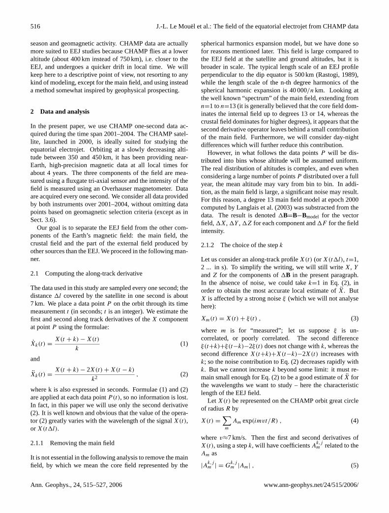
andj is the order of the derivative.Gk,jm is the gain factor

for the Ak,jm coefficient (seeOlsen, 2004). It is plotted as

a function of the wavelengthλ=2πR/m for j=2 and threedifferent values ofk on Fig.1. The maximum gain forj=2andk=20 s is 0.01 at wavelengthλmax=2kv≈280 km.

In the present paper we chosek=20 s, after checking thatthe results are stable for 15<k<25. For values ofk between15 s and 25 s, Eq. (2) provides us with a true spatial derivativewhich fits our needs. The daily variationSR and the ringcurrent field have far longer spatial length scales than the EEJfield and are eliminated (or at least much reduced) by theselected second derivative filter. (Moreover, part of the ringcurrent field is included in the main field model.)

Note: It is rather easy to determine that the minimum valueof k for the noise contribution to Eq. (2) is smaller comparedto X; to this aim, one takes the absolute value of the seconddifference in Eq. (2) and looks at the evolution of the resultswith k.

2.2 Computing the longitudinal component

Let us denote byb the anomaly vector after applying thealong-track second derivative (b=1B). Its components ingeocentric coordinates are1X, 1Y , and1Z. Its projectionon the direction of the main fieldB, i.e.

bl = b ·B|B|

, (7)

will be called the longitudinal component of the anomalyfield. We have that

bl = α1X + β1Y + γ 1Z , (8)

whereα, β and γ are the direction cosines ofB, i.e. thecosines of the angles betweenB and thex, y andz axes. Thelongitudinal componentbl is more suited to the study of theEEJ thanb, because it is much less affected by instrumen-tal noise due to uncertainties in attitude determination, andby field-aligned currents (which generate transverse fields).However, Cartesian components ofb also bring valuable in-formation, as will be seen in the following section.

It is possible to perform a very similar analysis using scalardata only.F can be

√X2+Y+Z2 or given by the scalar mag-

netometer. The along-track second derivative of the field in-tensity may be expressed as

1F = α1X + β1Y + γ 1Z + α1X + β1Y + γ 1Z . (9)

Due to the long wavelengths ofα, β, γ and the short wave-lengths of the EEJ field, the last three terms of the RHS of(9) are much smaller than the first three terms and thereforewe have that

1F ≈ bl . (10)

Figures

102

103

104

0

0.002

0.004

0.006

0.008

0.01

0.012

0.014

0.016

0.018

Wavelength λ (km)

Gai

n fa

ctor

λmax

Fig. 1. Gain factor of the along track second derivative as a function of the wavelength of

the signal, using a step k = 15 s (red curve), k = 20 s (blue curve) and k = 25 s (green

curve). The wavelength λmax ≈ 280 km associated with the maximum gain for k = 20 s is

indicated on the graph.

24

Fig. 1. Gain factor of the along-track second derivative as a func-tion of the wavelength of the signal, using a stepk=15 s (red curve),k=20 s (blue curve) andk=25 s (green curve). The wavelengthλmax≈280 km associated with the maximum gain fork=20 s is in-dicated on the graph.

Using X, Y , Z andF data, we have checked that there areonly very minor differences between maps computed from1F and maps computed frombl . In what follows we willshow results for the longitudinal component (7) only, butall maps have also been computed using the scalar secondderivative (9).

2.3 Averaging in space and time

We average both in time and space, trying to lose as littleinformation as possible. Time averaging, over time spansmuch longer than one day, is used to smooth the big day-to-day variability of the electrojet. It is also necessary to con-sider long time spans in order to have enough individual mea-surements to average both in time and space. Instrumentalnoise and instantaneous fields of various origins are alwayspresent. Although we usually consider all the data acquiredfrom 2001 to 2004, we sometimes use them after creating dif-ferent subsets (for example, 2001, 2002, 2003 and 2004), inorder to investigate the stability of different patterns of theirtemporal variations.

For a given subset, we distribute the data within bins ofsize 2.5◦

×2.5◦ in latitude and longitude, without sorting thealtitudes. The total number of bins is 10 368. For each bini, we compute the average ofX(P ) over all pointsP withinthe bin; the same is done forY andZ. This average value,represented by a colored pixel on the maps, is attributed tothe bini.

www.ann-geophys.net/24/515/2006/ Ann. Geophys., 24, 515–527, 2006


-0.02 -0.01 0.00 0.01 0.02

Fig. 2. Along track second derivative of the crustal field (in nT/s2) from data in 2001-2004,

longitudinal component.

25

Fig. 2. Along-track second derivative of the crustal field (in nT/s2)from data in 2001–2004, longitudinal component.

2.4 Removing the crustal field

The crustal field has energy in the same spatial frequencydomain as the EEJ, so the two fields cannot be separatedthrough their spectral content. However, the crustal fielddoes not change in time, contrary to the EEJ field, which canbe assumed to vanish around local time midnight. Therefore,the maps obtained by our analysis at local times around mid-night have no contribution from the EEJ, and the same crustalfield contribution than at any other local time. We take ad-vantage of this fact and of the adequate accuracy of our mapsof averaged quantities, to extract an averaged map computedfrom 21:00 LT to 03:00 LT, from the other maps, in order toeliminate the crustal field.

3 Results

3.1 Crustal field

As said earlier, processing the data relative to the night localtime – in fact from 21:00 LT to 03:00 LT – provides simplythe map of the lithospheric field (Fig.2). It is, of course, atransformed anomaly map, a map of the along-track secondderivative of the intensity anomaly (not the intensity of theanomaly), often considered when dealing with aeromagneticsurveys in which only the intensity is measured. Note thatthe auroral zones are hidden using an ad hoc mask. The samemask will be used in all the maps presented in the paper.

The map of Fig.2 is very stable, i.e. is the same whencomputed from different subsets of the four years of data. Itpresents the well-known drawbacks and advantages of thiskind of map. On the one hand, since the orbits are grosslymeridian, the fields of geological structures trending east-west are amplified and, due to the angle between the mainfield and the vertical, the anomalies are displaced in themeridian direction with respect to their sources. On the otherhand, anomalies can be decoalesced and made easier to in-terpret. Lithospheric anomaly maps have been derived from

CHAMP and Ørsted data byMaus et al.(2002), following theearlier maps based on MAGSAT data (Cohen and Achache,1990; Ravat et al., 1995). We will not discuss the lithosphericfield in this paper, which is devoted to the equatorial electro-jet field.

3.2 Variations with local time

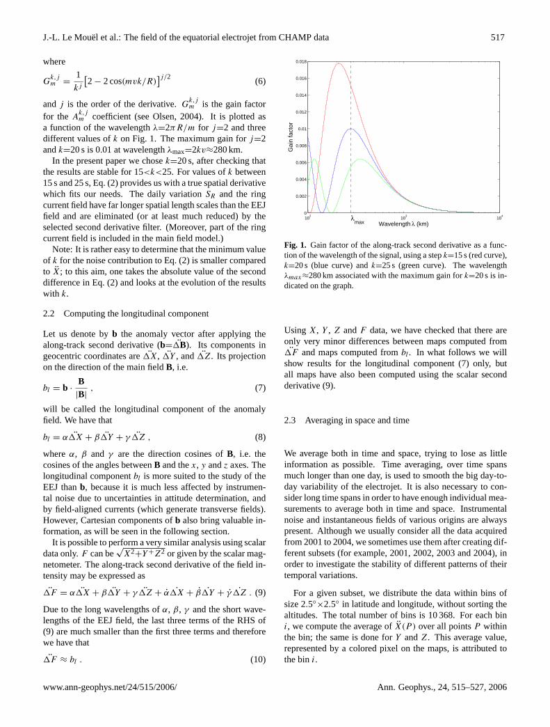
In order to study the variations with local time (LT) ofthe EEJ field, we split the data of the interval 2001–2004into 24 subsets, corresponding to the following LT intervals:00:30–01:30, 01:30–02:30, etc., 23:30–00:30. The maps forthe longitudinal component at 06:00, 08:00, 10:00, 12:00,14:00, 16:00 and 18:00 LT are shown in Fig.3. (Other mapsare not shown due to the limited space available.)

The map at 00:00 LT (Fig.3a) contains no EEJ signal.The remaining features, after removing the crustal field, areindeed very tiny and give an idea of the error in maps at otherlocal times.

A negative signal along the dip equator is visible at06:00 LT (Fig.3b). (In fact, it is already slightly visible onehour earlier). This signal is maximal over Africa, where itreaches−0.005 nT/s2 (i.e. about−10−4 nT/km2), but is ab-sent over the Pacific Ocean. It has been previously observedat ground stations in Africa, India and South America andis sometimes referred to as the morning counter electrojet(Gouin and Mayaud, 1967; Mayaud, 1977). The counterelectrojet disappears at 08:00 LT everywhere except overSouth America (Fig.3c).

Between 10:00 LT and 14:00 LT (Figs.3d–f), the full EEJsignal is visible. It is made of three parallel bands alignedand symmetrical with respect to the dip equator. Each bandhas an approximate width of 1000 km. The central band ispositive and is caused by the eastward equatorial electrojet.The two flanking bands are negative and of slightly lowerintensity; we will show in Sect. 3.5 that they are due to west-ward return currents. The intensity of the signal is maximalat 12:00 LT. Somewhat unexpectedly, it is slightly higherat 10:00 LT than at 14:00 LT. All three bands have abso-lute extrema between 0.005 and 0.02 nT/s2 (i.e. 10−4 and4×10−4 nT/km2) at 12:00 LT.

At 16:00 LT (Fig. 3g), the EEJ signal looks like that at08:00 LT, perhaps with a slightly stronger positive centralband. It is maximal over the Eastern Pacific Ocean, a regionwhere it is weak at 08:00 LT.

The dusk features of the EEJ are markedly different fromthe dawn features. At 18:00 LT (Fig.3h), the EEJ signal isalmost no longer visible. It is the green band along the geo-magnetic equator. There is no afternoon counter electrojet.

3.3 Variations with universal time

The variations with universal time (UT) are studied inthe same manner as the variations with local time, us-ing 24 subsets corresponding to UT intervals 00:30–01:30,



(a) (b)

(c) (d)

(e) (f)

(g) (h)

-0.02 -0.01 0.00 0.01 0.02

Fig. 3. Variation with local time of the along track second derivative of the equatorial elec-

trojet field (in nT/s2), longitudinal component, at 00:00 (a), 06:00 (b), 08:00 (c), 10:00 (d),

12:00 (e), 14:00 (f), 16:00 (g) and 18:00 (h).

26

Fig. 3. Variation with local time of the along-track second derivative of the equatorial electrojet field (in nT/s2), longitudinal component, at00:00(a), 06:00(b), 08:00(c), 10:00(d), 12:00(e), 14:00(f), 16:00(g) and 18:00(h).

01:30–02:30, etc., and applying the same analysis to the lon-gitudinal component. The result is an hour-by-hour movie ofthe EEJ displacement around the world. Expectedly, the EEJis made of the same three bands as in the LT maps and fol-lows the dip equator. Less expectedly, its length and intensity

varies significantly along its path. Due to the limited spaceavailable, only the maps at 06:00, 11:00 and 17:00 UT arepresented in Fig.4.

The EEJ at 06:00 UT (Fig.4a) is made up of three parts:a head at the western side, a body and a tail at the eastern



(a)

(b)

(c)

-0.02 -0.01 0.00 0.01 0.02

Fig. 4. Variation with universal time of the along track second derivative of the equatorial

electrojet field (in nT/s2), longitudinal component, at 06:00 (a), 11:00 (b) and 17:00 (c).

27

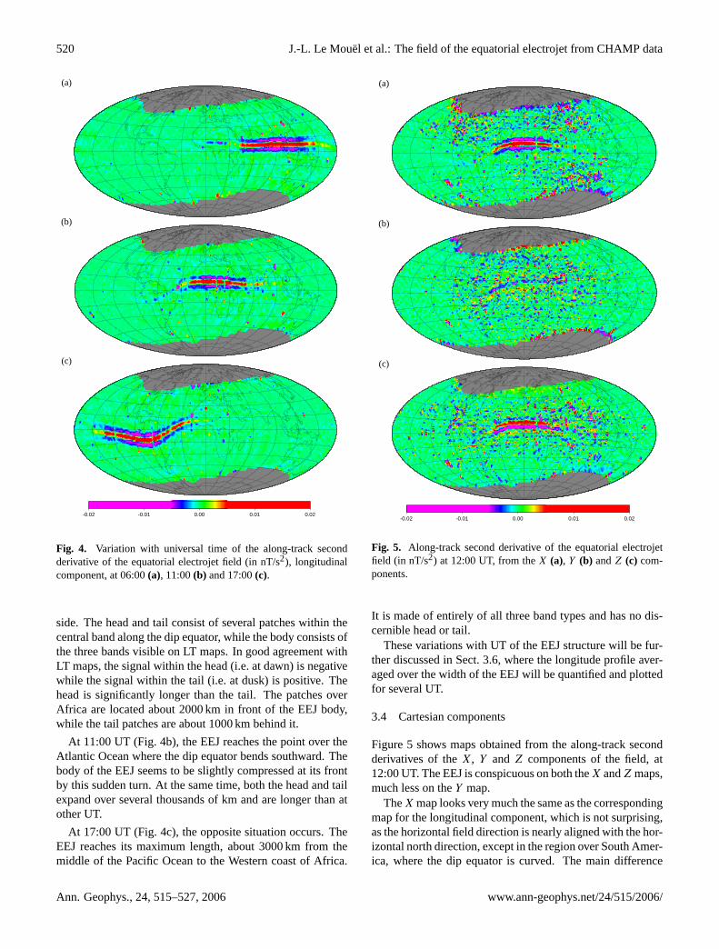
Fig. 4. Variation with universal time of the along-track secondderivative of the equatorial electrojet field (in nT/s2), longitudinalcomponent, at 06:00(a), 11:00(b) and 17:00(c).

side. The head and tail consist of several patches within thecentral band along the dip equator, while the body consists ofthe three bands visible on LT maps. In good agreement withLT maps, the signal within the head (i.e. at dawn) is negativewhile the signal within the tail (i.e. at dusk) is positive. Thehead is significantly longer than the tail. The patches overAfrica are located about 2000 km in front of the EEJ body,while the tail patches are about 1000 km behind it.

At 11:00 UT (Fig.4b), the EEJ reaches the point over theAtlantic Ocean where the dip equator bends southward. Thebody of the EEJ seems to be slightly compressed at its frontby this sudden turn. At the same time, both the head and tailexpand over several thousands of km and are longer than atother UT.

At 17:00 UT (Fig.4c), the opposite situation occurs. TheEEJ reaches its maximum length, about 3000 km from themiddle of the Pacific Ocean to the Western coast of Africa.

(a)

(b)

(c)

-0.02 -0.01 0.00 0.01 0.02

Fig. 5. Along track second derivative of the equatorial electrojet field (in nT/s2) at 12:00 UT,

from the X (a), Y (b) and Z (c) components.

28

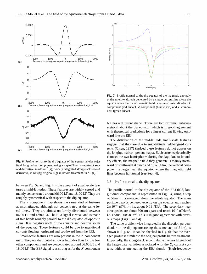
Fig. 5. Along-track second derivative of the equatorial electrojetfield (in nT/s2) at 12:00 UT, from theX (a), Y (b) andZ (c) com-ponents.

It is made of entirely of all three band types and has no dis-cernible head or tail.

These variations with UT of the EEJ structure will be fur-ther discussed in Sect. 3.6, where the longitude profile aver-aged over the width of the EEJ will be quantified and plottedfor several UT.

3.4 Cartesian components

Figure5 shows maps obtained from the along-track secondderivatives of theX, Y and Z components of the field, at12:00 UT. The EEJ is conspicuous on both theX andZ maps,much less on theY map.

TheX map looks very much the same as the correspondingmap for the longitudinal component, which is not surprising,as the horizontal field direction is nearly aligned with the hor-izontal north direction, except in the region over South Amer-ica, where the dip equator is curved. The main difference



(a)-2000 -1000 0 1000 2000Distance from magnetic equator (negative to S direction), km

-0.0001

0

0.0001

0.0002nT

/km

2

(b)-2000 -1000 0 1000 2000Distance from magnetic equator (negative to S direction), km

-12

-8

-4

0

4

8

nT

(c)-2000 -1000 0 1000 2000Distance from magnetic equator (negative to S direction), km

-24

-20

-16

-12

-8

-4

0

nT

Fig. 6. Profile normal to the dip equator of the equatorial electrojet field, longitudinal

component, using a step of 5 km: along track second derivative, in nT/km2 (a); twicely

integrated along track second derivative, in nT (b); original signal, before treatment, in nT

(c).

29

Fig. 6. Profile normal to the dip equator of the equatorial electrojetfield, longitudinal component, using a step of 5 km: along-track sec-ond derivative, in nT/km2 (a); twicely integrated along-track secondderivative, in nT(b); original signal, before treatment, in nT(c).

between Fig.5a and Fig.4 is the amount of small-scale fea-tures at mid-latitudes. These features are widely spread andmainly concentrated around 06:00 LT and 18:00 LT. They areroughly symmetrical with respect to the dip equator.

The Y component map shows the same kind of featuresat mid-latitudes, although not concentrated at the same lo-cal times. They are almost uniformly distributed between06:00 LT and 18:00 LT. The EEJ signal is weak and is madeof two bands roughly parallel to the dip equator, of oppositesigns. It is negative north of the equator and positive southof the equator. These features could be due to meridionalcurrents flowing northward and southward from the EEJ.

Small-scale features are also present in theZ componentmap. They are distributed at lower latitudes than for the twoother components and are concentrated around 06:00 LT and18:00 LT. The EEJ signal is as strong as for theX component

−30 −20 −10 0 10 20 30−4

−3

−2

−1

0

1

2x 10

−3

latitude (deg)

anom

aly

(no

unit)

Fig. 7. Profile normal to the dip equator of the magnetic anomaly at the satellite altitude

generated by a single current line along the equator when the main magnetic field is as-

sumed axial dipolar: X component (red curve), Z component (blue curve) and F compo-

nent (green curve).

30

Fig. 7. Profile normal to the dip equator of the magnetic anomalyat the satellite altitude generated by a single current line along theequator when the main magnetic field is assumed axial dipolar:X

component (red curve),Z component (blue curve) andF compo-nent (green curve).

but has a different shape. There are two extrema, antisym-metrical about the dip equator, which is in good agreementwith theoretical predictions for a linear current flowing east-ward like the EEJ.

The distribution of the mid-latitude small-scale featuressuggest that they are due to mid-latitude field-aligned cur-rents (Olsen, 1997) (indeed these features do not appear onthe longitudinal component maps). Such currents electricallyconnect the two hemispheres during the day. Due to bound-ary effects, the magnetic field they generate is mainly north-ward or southward at dawn and dusk. Also, the vertical com-ponent is larger near the equator where the magnetic fieldlines become horizontal (see Sect. 4).

3.5 Profile normal to the dip equator

The profile normal to the dip equator of the EEJ field, lon-gitudinal component, is represented in Fig.6a, using a stepof 5 km. It is averaged along the whole equator. The mainpositive peak is centered exactly on the equator and reaches2×10−4 nT/km2, i.e. about 0.01 nT/s2. The secondary neg-ative peaks are about 500 km apart and reach 10−4 nT/km2,i.e. about 0.005 nT/s2. This is in good agreement with previ-ous maps (Figs.3 and4).

The same profile, twice integrated in the direction perpen-dicular to the dip equator (using the same step of 5 km), isshown in Fig.6b. It can be checked in Fig.6c that the aver-aged profile is similar to the original profile before treatment.Expectedly, the along-track second derivative has filtered outthe large-scale variation associated with theSq current sys-tem, without attenuating the EEJ signal. (High-frequency



0 90 180 270 360−1

0

1

2x 10

−4

← Bangui anomaly

longitude

nT/k

m2

B" day−nightB" nightB" day

Fig. 8. Profile along the dip equator of the equatorial electrojet field, longitudinal compo-

nent (in nT/km2), using data from the whole interval 2001-2004 (in black); results obtained

without removing the crustal field, using data from 6 hours of day only (in red) and 6 hours

of night only (in blue). The anomaly is projected onto the normal to the dip equator and

then averaged over a 500 km wide and 1300 km long window sliding along the equator.

31

Fig. 8. Profile along the dip equator of the equatorial electrojet field,longitudinal component (in nT/km2), using data from the whole in-terval 2001–2004 (in black); results obtained without removing thecrustal field, using data from 6 h of day only (in red) and 6 h of nightonly (in blue). The anomaly is projected onto the normal to the dipequator and then averaged over a 500-km wide and 1300-km longwindow sliding along the equator.

0 90 180 270 360

0.5

1

1.5

2x 10

−4

longitude

nT/k

m2

B" 2001−2002B" 2003−2004

Fig. 9. Comparison of the longitude profiles of the equatorial electrojet field, longitudinal

component (in nT/km2), obtained from 2001-2002 data only (in black) and 2003-2004 data

only (in red).

32

Fig. 9. Comparison of the longitude profiles of the equatorial elec-trojet field, longitudinal component (in nT/km2), obtained from2001–2002 data only (in black) and 2003–2004 data only (in red).

noise is present in Fig.6c and not in Fig.6a because the dataare averaged over all longitudes without being averaged in2.5◦

×2.5◦ bins, as this is the case when producing Figs.6aand6b.)

Figures6b and c show that the main peak in the secondderivative curve corresponds exactly to the central peak ofthe raw field anomaly. The secondary peaks in the secondderivative curve are, as expected, slightly shifted from their

0 90 180 270 3600.4

1.4

2.4x 10

−4

nT/k

m2

longitude

B" am<9B" am>33

Fig. 10. Variation with geomagnetic activity of the longitude profile of the equatorial elec-

trojet field, longitudinal component, in nT/km2: am < 9 (in black), am > 33 (in red).

33

Fig. 10. Variation with geomagnetic activity of the longitude pro-file of the equatorial electrojet field, longitudinal component, innT/km2: am<9 (in black),am>33 (in red).

positions in the raw field curve, by about 250 km towards thedip equator. However, the ratio of intensities between thesepeaks and the main peak, about 2, is almost not affected bythe second derivative.

While the central band of the EEJ signal on the maps inFigs.3 and4 is clearly caused by an eastward electric currentalong the dip equator, the origin of the two flanking bands,visible from 08:00 LT to 16:00 LT, is less obvious. Theycould be caused by the eastward band of the current itself orby westward return currents on each side of the central east-ward current. To shed light on this issue, let us assume thatthe main field is axial dipolar (hence the dip equator and geo-graphic equator are the same) and consider a single eastwardcurrent line along the equator at the altitude 100 km. Linecurrent models are widely used in the literature (e.g.Fam-bitakoye and Mayaud, 1976), although they are often morecomplicated than this one. The field anomaly generated bythis current line at the altitude 400 km is calculated in Ap-pendix A and is represented as a function of the latitude inFig.7. There is no flanking high on theX andF components,because the profile is calculated well above the electric cur-rent line and the spherical geometry of the Earth is taken intoaccount. (The same calculation applied to a zero altitude in-deed leads to flanking highs.) The comparison of Figs.6band7 suggests that the two flanking bands require westwardreturn currents on each side of the central EEJ.

3.6 Profile along the dip equator

The longitude profile of the EEJ field, longitudinal compo-nent, is calculated using a 500-km wide and 1300-km longwindow sliding along the dip equator; 500 km is roughly thewidth of the uppermost part of the EEJ peak (see Fig.6a), and



(a)

0 90 180 270 360−1

0

1

2

x 10−4

longitude

nT/k

m2

B" 2001−2002B" 2003−2004

(b)

0 90 180 270 360−1

0

1

2

x 10−4

longitude

nT/k

m2

B" 2001−2002B" 2003−2004

(c)

0 90 180 270 360−1

0

1

2

x 10−4

longitude

nT/k

m2

B" 2001−2002B" 2003−2004

Fig. 11. Variation with universal time of the longitude profile of the equatorial electrojet

field, longitudinal component, in nT/km2. The profiles are computed over 2001-2002 (black

curves) and 2003-2004 (red curves) at 06:00 (a), 08:00 (b) and 22:00 (c).

34

(a)

0 90 180 270 360−1

0

1

2

x 10−4

longitude

nT/k

m2

B" 2001−2002B" 2003−2004

(b)

0 90 180 270 360−1

0

1

2

x 10−4

longitude

nT/k

m2

B" 2001−2002B" 2003−2004

(c)

0 90 180 270 360−1

0

1

2

x 10−4

longitude

nT/k

m2

B" 2001−2002B" 2003−2004

Fig. 11. Variation with universal time of the longitude profile of the equatorial electrojet

field, longitudinal component, in nT/km2. The profiles are computed over 2001-2002 (black

curves) and 2003-2004 (red curves) at 06:00 (a), 08:00 (b) and 22:00 (c).

34

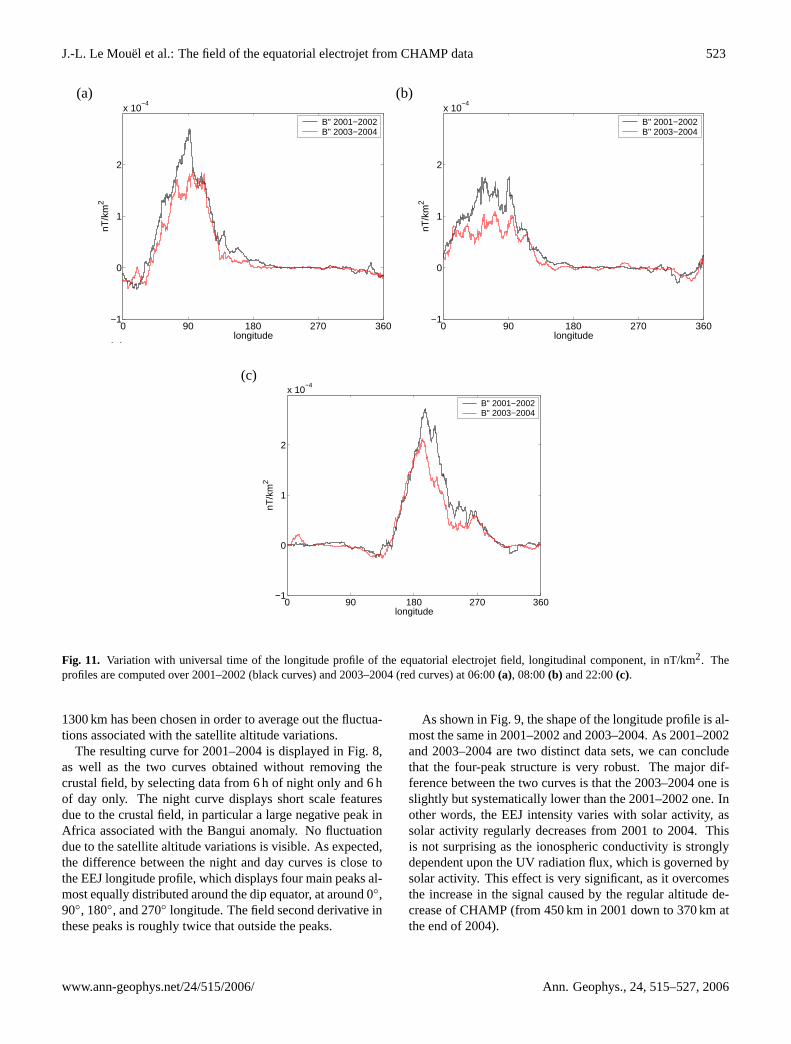
Fig. 11. Variation with universal time of the longitude profile of the equatorial electrojet field, longitudinal component, in nT/km2. Theprofiles are computed over 2001–2002 (black curves) and 2003–2004 (red curves) at 06:00(a), 08:00(b) and 22:00(c).

1300 km has been chosen in order to average out the fluctua-tions associated with the satellite altitude variations.

The resulting curve for 2001–2004 is displayed in Fig.8,as well as the two curves obtained without removing thecrustal field, by selecting data from 6 h of night only and 6 hof day only. The night curve displays short scale featuresdue to the crustal field, in particular a large negative peak inAfrica associated with the Bangui anomaly. No fluctuationdue to the satellite altitude variations is visible. As expected,the difference between the night and day curves is close tothe EEJ longitude profile, which displays four main peaks al-most equally distributed around the dip equator, at around 0◦,90◦, 180◦, and 270◦ longitude. The field second derivative inthese peaks is roughly twice that outside the peaks.

As shown in Fig.9, the shape of the longitude profile is al-most the same in 2001–2002 and 2003–2004. As 2001–2002and 2003–2004 are two distinct data sets, we can concludethat the four-peak structure is very robust. The major dif-ference between the two curves is that the 2003–2004 one isslightly but systematically lower than the 2001–2002 one. Inother words, the EEJ intensity varies with solar activity, assolar activity regularly decreases from 2001 to 2004. Thisis not surprising as the ionospheric conductivity is stronglydependent upon the UV radiation flux, which is governed bysolar activity. This effect is very significant, as it overcomesthe increase in the signal caused by the regular altitude de-crease of CHAMP (from 450 km in 2001 down to 370 km atthe end of 2004).



(a)

0 90 180 270 360

1

2

2.5x 10

−4

longitude

nT/k

m2

B" spring 2001−2002B" spring 2003−2004

(b)

0 90 180 270 360

1

2

2.5x 10

−4

longitude

nT/k

m2

B" summer 2001−2002B" summer 2003−2004

(c)

0 90 180 270 360

1

2

2.5x 10

−4

longitude

nT/k

m2

B" autumn 2001−2002B" autumn 2003−2004

(d)

0 90 180 270 360

1

2

2.5x 10

−4

longitude

nT/k

m2

B" winter 2001−2002B" winter 2003−2004

Fig. 12. Seasonal variation of the longitude profile of the equatorial electrojet field, lon-

gitudinal component, in nT/km2: spring (a), summer (b), autumn (c) and winter (d). The

profiles are computed over 2001-2002 (red curves) and 2003-2004 (black curves).

35

(a)

0 90 180 270 360

1

2

2.5x 10

−4

longitude

nT/k

m2

B" spring 2001−2002B" spring 2003−2004

(b)

0 90 180 270 360

1

2

2.5x 10

−4

longitude

nT/k

m2

B" summer 2001−2002B" summer 2003−2004

(c)

0 90 180 270 360

1

2

2.5x 10

−4

longitude

nT/k

m2

B" autumn 2001−2002B" autumn 2003−2004

(d)

0 90 180 270 360

1

2

2.5x 10

−4

longitude

nT/k

m2

B" winter 2001−2002B" winter 2003−2004

Fig. 12. Seasonal variation of the longitude profile of the equatorial electrojet field, lon-

gitudinal component, in nT/km2: spring (a), summer (b), autumn (c) and winter (d). The

profiles are computed over 2001-2002 (red curves) and 2003-2004 (black curves).

35

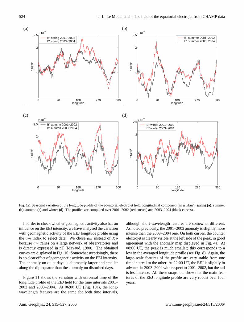
Fig. 12. Seasonal variation of the longitude profile of the equatorial electrojet field, longitudinal component, in nT/km2: spring(a), summer(b), autumn(c) and winter(d). The profiles are computed over 2001–2002 (red curves) and 2003–2004 (black curves).

In order to check whether geomagnetic activity also has aninfluence on the EEJ intensity, we have analysed the variationwith geomagnetic activity of the EEJ longitude profile usingthe am index to select data. We choseam instead ofKp

becauseam relies on a large network of observatories andis directly expressed in nT (Mayaud, 1980). The obtainedcurves are displayed in Fig.10. Somewhat surprisingly, thereis no clear effect of geomagnetic activity on the EEJ intensity.The anomaly on quiet days is alternately larger and smalleralong the dip equator than the anomaly on disturbed days.

Figure11 shows the variation with universal time of thelongitude profile of the EEJ field for the time intervals 2001–2002 and 2003–2004. At 06:00 UT (Fig. 10a), the long-wavelength features are the same for both time intervals,

although short-wavelength features are somewhat different.As noted previously, the 2001–2002 anomaly is slightly moreintense than the 2003–2004 one. On both curves, the counterelectrojet is clearly visible at the left side of the peak, in goodagreement with the anomaly map displayed in Fig.4a. At08:00 UT, the peak is much smaller; this corresponds to alow in the averaged longitude profile (see Fig.8). Again, thelarge-scale features of the profile are very stable from onetime interval to the other. At 22:00 UT, the EEJ is slightly inadvance in 2003–2004 with respect to 2001–2002, but the tailis less intense. All these snapshots show that the main fea-tures of the EEJ longitude profile are very robust over fouryears.



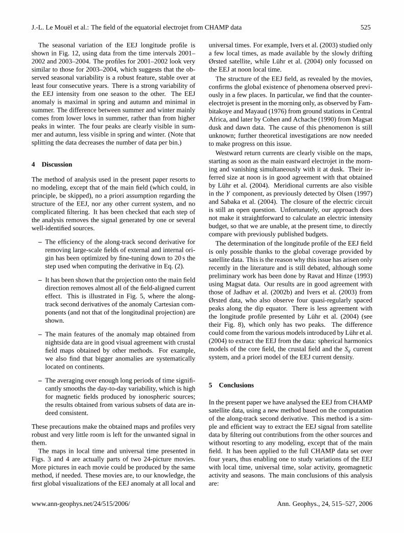
The seasonal variation of the EEJ longitude profile isshown in Fig.12, using data from the time intervals 2001–2002 and 2003–2004. The profiles for 2001–2002 look verysimilar to those for 2003–2004, which suggests that the ob-served seasonal variability is a robust feature, stable over atleast four consecutive years. There is a strong variability ofthe EEJ intensity from one season to the other. The EEJanomaly is maximal in spring and autumn and minimal insummer. The difference between summer and winter mainlycomes from lower lows in summer, rather than from higherpeaks in winter. The four peaks are clearly visible in sum-mer and autumn, less visible in spring and winter. (Note thatsplitting the data decreases the number of data per bin.)

4 Discussion

The method of analysis used in the present paper resorts tono modeling, except that of the main field (which could, inprinciple, be skipped), no a priori assumption regarding thestructure of the EEJ, nor any other current system, and nocomplicated filtering. It has been checked that each step ofthe analysis removes the signal generated by one or severalwell-identified sources.

– The efficiency of the along-track second derivative forremoving large-scale fields of external and internal ori-gin has been optimized by fine-tuning down to 20 s thestep used when computing the derivative in Eq. (2).

– It has been shown that the projection onto the main fielddirection removes almost all of the field-aligned currenteffect. This is illustrated in Fig.5, where the along-track second derivatives of the anomaly Cartesian com-ponents (and not that of the longitudinal projection) areshown.

– The main features of the anomaly map obtained fromnightside data are in good visual agreement with crustalfield maps obtained by other methods. For example,we also find that bigger anomalies are systematicallylocated on continents.

– The averaging over enough long periods of time signifi-cantly smooths the day-to-day variability, which is highfor magnetic fields produced by ionospheric sources;the results obtained from various subsets of data are in-deed consistent.

These precautions make the obtained maps and profiles veryrobust and very little room is left for the unwanted signal inthem.

The maps in local time and universal time presented inFigs. 3 and 4 are actually parts of two 24-picture movies.More pictures in each movie could be produced by the samemethod, if needed. These movies are, to our knowledge, thefirst global visualizations of the EEJ anomaly at all local and

universal times. For example,Ivers et al.(2003) studied onlya few local times, as made available by the slowly driftingØrsted satellite, whileLuhr et al.(2004) only focussed onthe EEJ at noon local time.

The structure of the EEJ field, as revealed by the movies,confirms the global existence of phenomena observed previ-ously in a few places. In particular, we find that the counter-electrojet is present in the morning only, as observed byFam-bitakoye and Mayaud(1976) from ground stations in CentralAfrica, and later byCohen and Achache(1990) from Magsatdusk and dawn data. The cause of this phenomenon is stillunknown; further theoretical investigations are now neededto make progress on this issue.

Westward return currents are clearly visible on the maps,starting as soon as the main eastward electrojet in the morn-ing and vanishing simultaneously with it at dusk. Their in-ferred size at noon is in good agreement with that obtainedby Luhr et al.(2004). Meridional currents are also visiblein theY component, as previously detected byOlsen(1997)andSabaka et al.(2004). The closure of the electric circuitis still an open question. Unfortunately, our approach doesnot make it straightforward to calculate an electric intensitybudget, so that we are unable, at the present time, to directlycompare with previously published budgets.

The determination of the longitude profile of the EEJ fieldis only possible thanks to the global coverage provided bysatellite data. This is the reason why this issue has arisen onlyrecently in the literature and is still debated, although somepreliminary work has been done byRavat and Hinze(1993)using Magsat data. Our results are in good agreement withthose ofJadhav et al.(2002b) and Ivers et al.(2003) fromØrsted data, who also observe four quasi-regularly spacedpeaks along the dip equator. There is less agreement withthe longitude profile presented byLuhr et al. (2004) (seetheir Fig. 8), which only has two peaks. The differencecould come from the various models introduced byLuhr et al.(2004) to extract the EEJ from the data: spherical harmonicsmodels of the core field, the crustal field and theSq currentsystem, and a priori model of the EEJ current density.

5 Conclusions

In the present paper we have analysed the EEJ from CHAMPsatellite data, using a new method based on the computationof the along-track second derivative. This method is a sim-ple and efficient way to extract the EEJ signal from satellitedata by filtering out contributions from the other sources andwithout resorting to any modeling, except that of the mainfield. It has been applied to the full CHAMP data set overfour years, thus enabling one to study variations of the EEJwith local time, universal time, solar activity, geomagneticactivity and seasons. The main conclusions of this analysisare:



P

r

Lγ

E AO

h S

RT

α

β

Fig. A1. Geometric notations used in the derivation of the field anomaly generated by a

single current line along the equator when the main magnetic field is assumed axial dipolar.

36

Fig. A1. Geometric notations used in the derivation of the fieldanomaly generated by a single current line along the equator whenthe main magnetic field is assumed axial dipolar.

1. The electrojet is made up of a central band of currentflowing eastward and two lateral, less intense, bands ofcurrent flowing westward; the total size of the EEJ isabout 2000-km width.

2. There exists a morning counter electrojet over a largefraction of the dip equator; there is no afternoon counterelectrojet.

3. The EEJ length varies along its path over the dip equa-tor; it is compressed when the equator bends southward.

4. Meridional EEJ currents are visible on theY compo-nent.

5. Small-scale features, which could be attributed to in-terhemispheric currents, are visible on theX, Y andZ

components at mid-latitudes.

6. The EEJ longitude profile displays four regularly spacedpeaks.

7. The EEJ intensity decreases with solar activity, whichsuggests that it is strongly dependent upon the UV radi-ation flux.

8. The EEJ does not vary with geomagnetic activity.

9. The EEJ is minimum in summer and maximum inspring and fall.

In a further study, we will compare our results with thosepredicted by the comprehensive model CM4 ofSabaka et al.(2004).

Appendix A

Field generated by a current line at satellite altitude

Let us consider a single eastward current line along the ge-ographic equator at an altitudehE=100 km and assume themain geomagnetic field is axial dipolar. The purpose of thisAppendix is to obtain the expression of the field anomalygenerated by this current line along the orbit of a CHAMP-like satellite, assumed to be polar and circular, at an alti-tude hS=400 km. This is a 2-D problem, to be solved inthe meridian plane; see Fig.A1.

The north and downward vertical components of theanomaly at a pointP on the orbit may be expressed as

1X = −µ0i

2πrsinα , (A1)

1Z = −µ0i

2πrcosα , (A2)

wherei is the current intensity,r the distance from the cur-rent line andα the angle between the anomaly field and thevertical direction atP . Then the scalar anomaly is

1F ≈ −µ0i

2πr(sinα cosI + cosα sinI ) , (A3)

whereI is the local inclination of the main field.In the case of an axial dipolar magnetic field, it is well-

known thatI may be related to the latitudeL using

I = arctan(2 tanL) . (A4)

Using classical trigonometric formulae, we find that

α =π

2− β + γ , (A5)

β =π − L

2, (A6)

γ = arctan

[1h sinβ

2(RT + hS) sin(

L2

)− 1h cosβ

], (A7)

whereRT is the Earth’s radius,1h=hE−hS andβ andγ areboth defined as in Fig.A1. Therefore, the angleα is given by

α =L

2− arctan

[1hcotan

(L2

)2(RT + hS) − 1h

]. (A8)

Substituting Eqs. (A4) and (A8) into Eq. (A3), we may cal-culate the profile of the anomaly due to the current line alongthe orbit of the satellite.



Acknowledgements.We thank T. Sabaka for his thorough readingof the manuscript and for his helpful suggestions. We thank S. Byr-dina for helping with the calculations. We thank P.-N. Mayaud formany interesting discussions. We also thank the two referees forhelpful comments. This is IPGP contribution No. 2114.

Topical Editor M. Pinnock thanks D. Ravat and another refereefor their help in evaluating this paper.

References

Cohen, Y.: Traitements et interpretations de donnees spatiales engeomagnetisme:etude des variations laterales d’aimantation dela lithosphere terrestre, Ph.D. thesis, Universite Paris VII, 1989.

Cohen, Y. and Achache, J.: New global vector magnetic anomalymaps derived from Magsat data, J. Geophys. Res., 95, 10 783–10 800, 1990.

Doumouya, V., Vassal, J., Cohen, Y., Fambitakoye, O., and Men-vielle, M.: Equatorial electrojet at African longitudes: first re-sults from magnetic measurements, Ann. Geophys., 16, 658–676, 1998,SRef-ID: 1432-0576/ag/1998-16-658.

Egedal, J.: The magnetic diurnal variation of the horizontal forcenear the magnetic equator, Terr. Magn. Atmos. Electr., 52, 449–451, 1947.

Fambitakoye, O. and Mayaud, P. N.: Equatorial electrojet and reg-ular daily variationSR ; II, the center of the equatorial electrojet,J. Atmos. Terr. Phys., 38, 19–26, 1976.

Forbes, J. M.: The Equatorial Electrojet, Rev. Geophys. SpacePhys., 19, 469–504, 1981.

Forbush, S. E. and Casaverde, M.: Equatorial Electrojet in Peru,Tech. Rep. 620, Carnegie Inst. Wash., Washington, D.C., 1961.

Gouin, P. and Mayaud, P. N.: A propos de l’existence possible d’un“contre electrojet” aux latitudes magnetiquesequatoriales, Ann.Geophys., 23, 41–47, 1967.

Ivers, D., Stening, R., Turner, J., and Winch, D.: Equatorial electro-jet from Ørsted scalar magnetic field observations, J. Geophys.Res., 108(A2), 1061, doi:10.1029/2002JA009310, 2003.

Jadhav, G., Rajaram, M., and Rajaram, R.: Main field control of theequatorial electrojet: a preliminary study from the Oersted data,J. Geodyn., 33, 157–171, 2002a.

Jadhav, G., Rajaram, M., and Rajaram, R.: A detailed study of equa-torial electrojet phenomenon using Ørsted satellite observations,J. Geophys. Res., 107(A8), 1175, doi:10.1029/2001JA000183,2002b.

Langel, R. A., Purucker, M., and Rajaram, M.: The equatorial elec-trojet and associated currents as seen in Magsat data, J. Atmos.Terr. Phys., 55, 1233–1269, 1993.

Langlais, B., Mandea, M., and Ultre-Guerard, P.: High-resolutionmagnetic field modeling: application to MAGSAT and Ørsteddata, Phys. Earth Planet. Inter., 135, 77–91, 2003.

Luhr, H., Maus, S., and Rother, M.: Noon-time equatorial electro-jet: Its spatial features as determined by the CHAMP satellite,J. Geophys. Res., 109, A01 306, doi:10.1029/2002JA009656,2004.

Maus, S., Rother, M. amd Holme, R., Luhr, H., Olsen, N., andHaak, V.: First scalar magnetic anomaly map from CHAMPsatellite data indicates weak lithospheric field, Geophys. Res.Lett., 29(14), doi:10.1029/2001GL013685, 2002.

Mayaud, P. N.: The equatorial counter electrojet – A review ofits geomagnetic aspects, J. Atmos. Terr. Phys., 39, 1055–1070,1977.

Mayaud, P. N.: Derivation, Meaning and Use of Geomagnetic In-dices, Geophysical Monograph 22, Am. Geophys. Union, Wash-ington, D.C., 1980.

Olsen, N.: IonosphericF region currents at middle and low latitudesestimated from Magsat data, J. Geophys. Res., 102(A3), 4563–4576, 1997.

Olsen, N.: Swarm End-to-End Mission Performance SimulatorStudy, Tech. rep., Danish Space Research Institute, ESA contractNo. 17263/03/NL/CB, 2004.

Rastogi, R. G.: The Equatorial Electrojet: Magnetic and Iono-spheric Effects, in Geomagnetism, edited by: Jacobs,J. A., vol. 3,chap. 7, Academic Press, London, 461–525, 1989.

Ravat, D. and Hinze, W. J.: Considerations of variations in iono-spheric field effects in mapping equatorial lithospheric Magsatmagnetic anomalies, Geophys. J. Int., 113, 387–398, 1993.

Ravat, D., Langel, R. A., Purucker, M., Arkani-Hamed, J., and Als-dorf, D. E.: Global vector and scalar Magsat magnetic anomalymaps, J. Geophys. Res., 100(B10), 20 111–20 136, 1995.

Rigoti, A., Chamalaun, F. H., Trivedi, N. B., and Padilha, A. L.:Characteristics of the equatorial electrojet determined from anarray of magnetometers in N-NE Brazil, Earth Planets Space,51, 115–128, 1999.

Sabaka, T. J., Olsen, N., and Langel, R. A.: A comprehensive modelof the quiet-time, near-Earth magnetic field: phase 3, Geophys.J. Int., 151, 32–68, 2002.

Sabaka, T. J., Olsen, N., and Purucker, M.: Extending compre-hensive models of the Earth’s magnetic field with Ørsted andCHAMP data, Geophys. J. Int., 159, 521–547, 2004.


http://direct.sref.org/1432-0576/ag/1998-16-658

the field of the equatorial electrojet from champ data

Documents