IZA DP No. 3953

The Financial and Operating Performance ofPrivatized Firms in Sweden

Motasam TatahiAlmas Heshmati

DI

SC

US

SI

ON

PA

PE

R S

ER

IE

S

Forschungsinstitutzur Zukunft der ArbeitInstitute for the Studyof Labor

January 2009

The Financial and Operating

Performance of Privatized Firms in Sweden

Motasam Tatahi European Business School London

Almas Heshmati Seoul National University

and IZA

Discussion Paper No. 3953 January 2009

IZA

P.O. Box 7240 53072 Bonn

Germany

Phone: +49-228-3894-0 Fax: +49-228-3894-180

E-mail: iza@iza.org

Any opinions expressed here are those of the author(s) and not those of IZA. Research published in this series may include views on policy, but the institute itself takes no institutional policy positions. The Institute for the Study of Labor (IZA) in Bonn is a local and virtual international research center and a place of communication between science, politics and business. IZA is an independent nonprofit organization supported by Deutsche Post World Net. The center is associated with the University of Bonn and offers a stimulating research environment through its international network, workshops and conferences, data service, project support, research visits and doctoral program. IZA engages in (i) original and internationally competitive research in all fields of labor economics, (ii) development of policy concepts, and (iii) dissemination of research results and concepts to the interested public. IZA Discussion Papers often represent preliminary work and are circulated to encourage discussion. Citation of such a paper should account for its provisional character. A revised version may be available directly from the author.

IZA Discussion Paper No. 3953 January 2009

ABSTRACT

The Financial and Operating Performance of Privatized Firms in Sweden

This paper examines the change in operating and financial performance of Swedish firms that were either partly or fully privatized during the period of 1989-2007. Two different methods are used to empirically investigate the performance of privatized firms. First, accounting data prior to and after the privatization are employed to measure the operating performance of privatized firms. We have found no significant difference in performances under state and private ownerships. Second, a return-based event study is found useful to measure the financial performance of privatized firms, since all the firms in the sample that were privatized have used an initial public offering (IPO). This approach allows comparison to the rest of the IPOs that were launched in the same period. It is found that the cumulative returns for the privatized firms are significantly different to private counterparts. Overall results, however, show that the privatization in Sweden was not as successful as it might have been expected and in comparison with those in other countries. JEL Classification: C12, D21, L25, L33 Keywords: Sweden, efficiency, performance measure, privatization, ratio analysis,

event-study, public and private relationship Corresponding author: Almas Heshmati College of Engineering TEMEP #37-306 Seoul National University San 56-1 Shilim-dong Kwanak-gu Seoul 151-742 Korea E-mail: heshmati@snu.ac.kr

1. Introduction The last 20 years have witnessed privatization programs on a global scale in both developed and developing countries. Different political parties with different ideological backgrounds have strongly pursued the change from state socialism with state-owned enterprises (SOE) to market based capitalism. The OECD (2003) estimated that over the past two decades, more than 100 countries worldwide have adopted privatization policies. Megginson et al. (1996) have emphasised that revenues from privatization through initial public offerings (IPO) have reached US $400 billion since 1979 and are expected to grow with an equal pace. According to Gibbon (1998), $860 billion has been raised by the governments worldwide through selling state owned enterprises since 1987. Roche (1996) predicts that no less than $6 trillion will be raised through privatizations over the next two decades. In 1997 alone, sales of public enterprises reached a total record of $161 billion worldwide. Many European countries have launched privatization programs since 1980. Among them, Great Britain is referred to as the origin of modern privatization: Margaret Thatcher’s government privatized many state-owned enterprises, including British Petroleum in 1979, British Telecom and British Airways. In France, privatization was very dependent on the political situation and the political party in the power. The first privatization started in 1986 with Elf Aquitaine. It was discontinued until 1993 when the socialist government left the office (see Schneider and Hofreither, 1990). In most industrialised economies, privatization policies have been promoted on the grounds that it improves the efficiency of SOEs, raises large amounts of revenues for the government and promotes general public’s share ownership in cases where companies are sold by shares to the public. There is a view that all government intervention in the market place represents some restriction to individual liberty and, hence, is intrinsically undesirable. This withdrawal of state involvement in industry, which came to be known as ’privatization’, takes place through a number of policy initiatives. The most common is a change from public to private in the ownership of an enterprise (or part of an enterprise). Alternatively, public enterprise may remain in existence while privatization takes place without transfer of ownership of assets. Falling into this category are liberalization involving deregulation of controls on entry, price, output and profit, as well as the adoption of a commercial approach. According this approach, the provision of a goods or service moves from the public to the private sector, but with ultimate responsibility for providing the service remaining with the government, frequently referred to as “contracting-out”. Positive views of privatization point to a number of benefits resulting from its adoption. Because privatization undermines the role of the unions, it permits a tough labour policy, which deals with the problems caused by inefficient workers, and thereby makes controlling employment levels much easier. It also permits the public sector economy to become familiar with ‘the enterprise culture’ as well as with the mechanism of the market place, leading to the rationalization of asset portfolios and the strategic reorganization of investment. This in turn leads to improvement of the

2

company’s balance sheets, introducing sensitivity and product quality improvement while providing adequate facilities for merging as required by the economics of international competition. Furthermore, since public managers and politicians may act in favour of each other, issues such as wage levels, investment plans, borrowing requirements and restructuring projects are assumed to be resolved by this internal relationship. Privatization supposedly breaks up this relationship and introduces a more efficient process of decision-making. A final argument in favour of privatization identifies a number of financial benefits to the policy. Firstly, the sale of public enterprises results in the removal of their capital investment programs from the public sector accounts; consequently, public sector borrowing is reduced. Secondly, it has been argued that private companies have more direct and faster access to the international capital market than public companies do. Thirdly, privatization contributes to the growth of the stock exchange, and can widen the capital market by bringing in many new investors. Fourthly, privatization helps to minimise the commercial risk, and therefore reduces economic problems for the government in different periods, especially when the market is volatile or in recession. It seems, however, that the above principle does not apply to private companies. It should be noted that, the limited evidence from the recent financial crisis shows that the state is invited to intervene in the private market to rescue banking, automobile and real estate markets in crisis to stabilize the financial market and to prevent bankruptcies and subsequent increasing unemployment. In terms of theoretical literature a large amount have dealt with the consequences of privatizations in terms of efficiency gains, different incentive structures, and increased competitive pressure, only a few empirical studies look at privatization programs either on a national or international scale. Among the empirical studies on the post-privatization performance several World Bank studies appear as the most comprehensive studies (see Galal et al., 1994; Megginson et al., 1994; Megginson et al., 1996; and Boubakri and Cosset, 1998). The first study analyzes the post-privatization performance of 12 companies from the most regulated industries in Britain, Chile, Malaysia, and Mexico. The World Bank did look at the economic consequences of privatization from an international perspective. The second study compared the pre- and post-privatization financial and operating performance of 61 companies from 18 countries and 32 industries that either experienced a full or partial privatization through public share offerings during the period of 1961-1990. The third study took an international perspective and its focus was more on privatization programs in developed countries. In contrast, the last study focused on the financial and operating performance of newly privatized firms in developing countries. In spite of these differences to the other studies, they also found that the performance of the enterprises showed significant improvements after their privatization. In this paper we look at the financial and operating performance of privatized firms in Sweden. A large-scale privatization program took place from 1989, when shares of the SSAB, one of Sweden’s heavy enterprises within the manufacturing sector, were sold at the Stockholm Stock Exchange. The SSAB was followed by firms like the Celsius AB, AssiDoman AB and Pharmacia AB. Until now, many of the large state owned

3

enterprises, apart from very few like Nordea Banken AB, are being privatized by selling shares. We firstly analyzed accounting data of those Swedish enterprises that experienced either a full or partial change in government ownership through an Initial Public Offering. This data is used to evaluate their performances prior to and after the privatization. What we have found does not support the studies cited above. Strong empirical support for improvements in profitability, efficiency, and other financial variables is not found. This can be conclusive that the operating performance of privatized firms has not been very strong. One of the reasons for these empirical findings can be referred to the type of privatization that largely occurred in Sweden. This can be attributed to the fact that, among the ten firms present in the sample, none of those firms experienced full privatization. This might refer to the influence of the state and conclude that it is still strong, and might account for the results. The second step of analysing, the pre-and-post privatization performance, involves using share prices of the privatized firms and it calculate returns to measure the financial performance on the basis of cumulative excess returns. The cumulative abnormal returns of the privatized firms are compared to those firms that experienced an IPO during the same period. The result shows that the abnormal returns of the privatized firms are significantly different from those of the regular IPO firms. The rest of this article is organized as follows. In the next section, theories in favour of privatization will briefly be discussed. The third section is devoted to the data and the methodology used for testing the hypothesis to measure the operating and financial performance. Section 4 presents the results for the operating performance of firms. Section 5 evaluates the financial performance of privatized firms on the basis of abnormal returns, and Section 6 concludes the study. 2. Theory There are several different schools of thought in favour of privatization, each of which addresses one particular aspect of this economic adjustment. It is worth emphasising that these schools unlike their recent application date as far back as 1870. Thus, schools of thought on privatization can be divided into two categories based on when they emerged. The first category consists of the Austrian School, the Property Rights School and the Public Choice School. The second category, which refers to recent ideas, is comprised of the Principal-Agent Theory, the New Political Economy, the New Austrian School of Economics and the New Institutional Economics. The property rights analysis of public ownership leads to the conclusion that public enterprises are less economically efficient than private enterprises. Thus, forms of ownership generate different rewards/penalties. Generally, the more dispersed property rights are, the less motivated their holders will be to use their assets efficiently. Moreover, according to the property rights school, the separation of ownership and management, which is characteristic of the modern corporation, does not lead to any fundamental change in the performance of private enterprise. It acknowledges that

4

shareholders in a large corporation are not able to monitor management as closely as a manager-owned company, but asserts that there are other factors at work in the modern corporation that compensate for this. The public choice perspective, like the theory of property rights, holds very strong views about public ownership. The fact that ‘public enterprises necessarily perform less efficiently than private enterprises,’ Starr (1989: 31) provides an influential economic case for privatization. Privatization allows profit-maximising decision-making to take place. Under public ownership, political motives, which lead to large subsidies and other concessions, are much more important than cost efficiency. Key public officials and ministers may pursue higher goals than operational efficiency leading to a higher cost of production. By contrast, privatization frees an enterprise from the burden of political interference and non-market criteria. Thus it limits politicians’ ability to redirect the enterprise’s activities in order to promote their personal agenda or to yield short-term political pressures at the expense of market efficiency. This clarifies the objectives of the enterprise and leads to the enhancement of economic performance. The Austrian school points to the fact that continual changes over time in tastes, techniques, available resources, prices, plans and expectations require that individuals (economic agents) be allowed to arrange their property as they see fit, in order to gain access to more and better knowledge than would be possible with less freedom of action (Moldofsky, 1989). The welfare of economic agents is improved in a competitive market which allows them to learn what consumers want, how much they are willing to pay, what factors and methods of production are available and so on. This process continuously ensures that resources are reallocated to new preferable uses in the best possible way. The competitive market provides an environment in which products will be produced by someone who can do so more cheaply than anybody who does not produce it, and that each product is sold at a lower price, (Hayek, 1984). The competitive market, whose foundation is price and shared economic knowledge, can generally only exist in the context of private ownership. It follows that privatization, via the introduction of competition, will improve efficiency and sensitivity to consumer demand, with a better quality and range of goods and services (Littlechild, 1986). Principal-agent theory also views critically the state–owned enterprises. It asserts that, in the case of public enterprises, there is no efficient mechanism by which the principals (the public) can control the actions of their agents (government officials); thus, inefficiency is allocated to state enterprises. In general, the agents pursue their own goals in a world of information asymmetries, incomplete contracts and the absence of clear objectives. If the reverse were the case, then the ownership would be a problem and agents could have acted according to contracts. Moreover, because the incentive is weak and unrelated to the profit motive in state enterprises, agents have no enthusiasm to achieve the highest efficiency level (Bos, 1991). In contrast, private ownership sets a precise restriction on the managerial behaviour by linking it to expected future profits. If profits are expected to decline, it will squeeze share prices and increase takeover bids. Large shareholders clearly know the consequences of poor managerial performance; hence they have enough incentive to motivate managerial behaviours. More importantly, because managerial salaries in the private sector are linked to profit,

5

stock options and bonuses, while in the public sector it is tied to fixed salary scales, the managerial motives will differ leading to different effort and outcomes. The new political economy sees rent seeking behaviour from government intervention into the market. It also sees these interventions as destroying a perfectly competitive environment. The new institutional economics sees the internal organisation of the firm as separate from its external market relations. It also sees that the economic agent has limited power to obtain all available information and that market transactions are not costless. Non-market institutions cannot act optimally, but individuals can. The neo-Austrian school of economics, unlike the two other schools sees the market economy as a dynamic phenomenon in an uncertain and changing world. Individual economic agents are assumed to be the main source of decision-making; that decision-making is based on all the information and knowledge they are able to obtain. The most important conclusions that can be extracted from the study of these three newly founded schools of thought are that: 1. The characteristic of the new ownership is much more important than the role

played by competition and regulation.

2. Private sector economy and, in this regard, privatization are much more favourable than public sector economy.

3. All the above schools are in favour of privatization and see the adjustments from the public to the private sector as a significant movement for enhancing the economy as a whole.

3. Data and Methodology The data of public enterprises, which were privatized, partially or fully, as IPOs at the Stockholm Stock Exchange are collected. The time period was chosen between 1989 and 2007. As a consequence of these selection criteria, 10 firms are included in the sample. As can be seen in Table 1, the Swedish government has emphasised to privatize public enterprises of different sizes and operating in different sectors of the economy such as manufacturing, forest industry, pharmaceutical, finance and banking industry, media industry, and services including hotel, and telecommunications. The variation in the initial value of transactions is large and lies in the interval $73.4 and $7,646.4 million (see Table 2).

Insert Table 1 and 2 about here The following approach is used to measure the operating performance of these firms. Based on accounting data that were collected from business reports, either from the Stockholm Stock Exchange or direct information from those enterprises or DataStream, we have carried out our analysis. These data are then adjusted for inflation. The monetary variables are transformed into fixed prices by using consumer price index. A number of accounting ratios that are appropriate for evaluating the performance of

6

firms prior to and after the privatization are employed. Those ratios are used for measuring (i) profitability, (ii) operating efficiency, (iii) capital investment, (iv) capital structure, (v) employment level, and (vi) liquidity of firms. Profitability is measured in three different ways as returns on sales, equity and investment. Two operating efficiency measures are obtained as sales per employee and net income efficiency. Capital investment is measured as capital expenditure to sales and to total assets, while capital expenditure is computed as equity ratio and as structure of short-term debt. The ratios are summarised in detail in Table 3.

Insert Table 3 about here These eleven performance criterion are used to evaluate the financial performance of those privatized firms. An event study is accomplished to evaluate each firm’s equity return performances through looking at the shares’ abnormal returns. To assess the performance changes of privatized firms the descriptive statistics is discussed in details. To test whether or not a statistically significant change after privatization took place, two tests are carried out: (i) the Wilcoxon test and (ii) the Standard test for differences in the mean performance of the two populations. The Wilcoxon singed rank test, which is a parameter free test, is especially well-suited for cases with small sample sizes. Two periods are identified; one prior to privatization as one population and after privatization as the second one for carrying out the second test to identify differences in the mean of the two populations. Despite the fact that the assumptions underlying the Wilcoxon test are always satisfied, the proper application of the test for differences in the mean of two populations requires the assumption of normal distributions. Consequently, this test should only be considered as complementary to the parameter free Wilcoxon test. Abnormal returns generated during the period of the IPO are used as procedure for measuring the financial performance of the firms. What was being considered most was to examine whether or not privatized firms display statistically different cumulative abnormal returns compared to other private IPOs that were undertaken during the same period. Firms that were privatized as IPOs at the Stockholm Stock Exchange are being considered as our broad data set. The time period was chosen between 1989 and 2007. Companies which are declined from the Stockholm Stock Exchange (Pharmacia and Rezidor Hotel Group) are excluded from our sample. The final sample consists of 8 privatized IPOs and 9 private IPOs. The sample chosen for the evaluation of the financial performance and their time of IPO is shown in Table 4.

Insert Table 4 about here 4. Operating Performance of Privatized Firms Schools of thought, as well as politicians in favour of privatization, have pointed to the productivity growth and the allocative efficiency under private ownership, compared

7

with public enterprises under public ownership. Theories such as the property rights theory, the public choice theory, the principal-agent theory, the Austrian school of economics, as well as some new theories like the new political economics, the new institutional economics and the neo-Austrian school of economic generally favour private ownership and view state ownership as inefficient, especially when the market is characterized as competitive. We consider, as the first step, the following hypotheses to test whether or not these expectations are met. As the second step, we look at the change in performance, on average over the last two years before and the first two years after privatization. Table 5 summarises the state of the 11 performance indicators for individual years and average period results before and after privatization.

Insert Table 5a and 5b about here A. Profitability It has been claimed that privatization will lead to change in economic prospects and it will allow profit-maximising entrepreneurs to be the main source of economic performance. Operational efficiency is guaranteed, leading to a lower cost of production. Political pressures to redirect the enterprise’s activities at the expense of market efficiency will be eliminated. Large subsidies and other special economic considerations will be minimised and the search for ways to reduce costs will no longer be necessary. All these remedies lead to enhanced economic performance. Hence, we expect the profitability to increase after privatization took place. To measure profitability return on sales, return on equity and return on assets are chosen. On average, all of these ratios have improved after privatization for the first year, and for the second year they have declined again to levels below their pre-privatization levels but despite deteriorated condition the period averages suggest small improvement in profitability. B. Operating Efficiency Private ownership is believed to improve corporate performance through incentives, and market phenomena are seen as disciplinary mechanisms for allocating resources efficiently. Moreover, the idea that the public sector acts against the public interest and efficiency - while the private sector is controlled by market discipline, the public sector serves the interests of managers or politicians. In the presence of market discipline, the role of the entrepreneurial factor in the market and relaxation of any barriers is believed to improve entrepreneurs’ behaviours. Further to this, it is claimed that creating greater competition is assumed to be more important than ownership. As a consequence, we anticipate efficiency to increase after privatization took place. To measure this efficiency is measured by means of two ratios, sales and profit per employee. Sales per employee decreased within the period before and after privatization. As far as profits per employee are concerned, there was a positive change from losses to significant profits after privatization. C. Capital Investment Theoretically, one can argue that private firm investment is based on a net present value

8

principle. From this view point, it may not be the case as far as state-owned enterprises are concerned. National governments, however, have utilised state-owned enterprises as an instrument to accelerate slow growing economies by additional investment spending. As a result of that public firms always had the credit rating as such to borrow almost unlimited funds at prime rates. These would suggest that investment spending is higher under state ownership as well as privatized firms compared with private ones. Hence, we assume that investment spending will increase for privatized firms. To evaluate this hypothesis we use two alternative measures: capital expenditure to sale and capital expenditure to total assets. As Table 5a shows both ratios have increased after privatization has taken place and then decreased again with small net positive effect. D. Capital Structure We assume that privatization will lead to reduced level of debt. This is based on the fact that a state-owned enterprise has much more debt capacity than a private firm. Furthermore, the credit rating of public firms is assumed to be higher than for private ones, given no-default risk of government activities. Hence, privatized firms would experience lower ratings and higher costs of debt. The increased costs of debt will result in the firms adjusting their capital structures. The financial performance is measured by means of two financial variables; the equity ratio, which measures equity as percentage of total assets, and a measure for short term debt (short term debt as percentage of total debt). This study shows that the equity ratio increased, and the rate of debt declined after privatization. Short-term debts were declined after privatization and have increased again afterward. E. Employment To measure the allocative performance of privatized firms, the employment level prior to and after the privatization is used. The aim is to examine whether or not efficiency gains result from reductions in the labour force. From theoretical view points, as priority is given to minimise the cost in the initial step, in the short run, the level of employments will slump. However, in the long-run as the cost efficiency results in lower production costs, the number of employment will increase. We found that the level of employment has increased in the first year of privatization and it has declined substantially afterward. F. Liquidity Liquidity is used as our final measure. It was increased meeting expectations of increased cash flows. The descriptive statistic results hint at an improvement in the profitability, productivity somehow and allocative performance of enterprises after privatization. The test results are in line with what we could expect from our descriptive statistics reported in Table 5a and 5b. In Table 6, we present the results of the Wilcoxon test of zero median vs non-zero median. We show the test statistics and the corresponding critical values for a significance level of 5%.

9

We work with the null hypothesis that there is no significant difference between the 11 ratios measuring profitability, efficiency, investment spending, capital structure, employment, and liquidity before and after privatization. The Wilcoxon test shows that all of those measures for which the null hypothesis, the median is zero, must be rejected and with the exception of liquidity all tests are statistically significant. Hence, from a statistical point of view, profitability, productive as well as allocative efficiency have been improved after privatization.

Insert Table 6 about here 5. Financial Performances of Privatized Firms 5.1 Event Study Methodology An event study is deployed to evaluate the financial performance of privatized firms compared with the private firms listed in the Stockholm Stock Exchange in the same period. This can be a useful method, since all the privatized firms included in our sample are stock listed companies through an IPO. The long-run performance of the IPOs is considered on the basis of abnormal returns for the privatized and at the same time their private firm counterparts. For each firm in the sample, the abnormal return is defined as the difference between the actual ex post stock return and the normal return (see McKinley, 1997). Thus, for firm i and in time period t the abnormal return is obtained as:

)( tititit XRERAR −= (1) where is the abnormal return, and itAR itR )( tit XRE are the actual and normal returns for time t, respectively, and Xt represents the conditioning information for the return model.

For measuring the normal return the market model is deployed. The return of any given security is conditioning on the return of the market portfolio. Moreover, a stable linear relation between these two returns is assumed. For any security, the market model states that the actual return of a given security at time t is:

itmtiiit RR εβα ++= (2) where Rmt is the time t return of the market portfolio, αi and βi are market model parameters and εit is a normally distributed zero mean disturbance term with variance

, i.e., 2itσ itε ~N(0, ) . 2

itσ Our sample of firms consists of 10 private firms and 10 state-owned firms that were

10

privatized during the years 1989 to 2007. For making our approach straightforward, we denote private firms as type 1 firms and the state-owned firms as type 2 firms. Moreover, we will introduce the following indexing of returns to make progress in the measurement and the analysis of abnormal returns. The time period t (t=1, 2, ....., T) is divided into three sub-periods: estimation window, event window and post-event window where the sub-periods thresholds are marked by T0, T1, T2 and T3. Defining t=0 as the IPO date, the estimation window of length L1=T1-T0 is from T0+1 through T1, the event window of length L2=T2-T1 from T1+1 through T2, and the length L3=T3-T2 ranging from T2+1 through T3 constitutes the post-estimation window. L1 and L2 are assumed to be the length of the estimation window and the post-estimation window, respectively. Three different estimation window lengths of 200, 400, and 750 days for both types of firms are used, i.e., L1=200, 400, 750, to estimate the market model parameters of the normal return for a given stock in the sample. The estimation of our regression parameters is based on the Swedish Traded Index (STX) which serves as the comparative market index. The ordinary least squares (OLS) regression method is selected to estimate the market model parameters. For firm i, for instance, the OLS estimators for the estimation window are:

∑

∑

+=

+=

−

−−=

10

10

12

1

)ˆ(

)ˆ)(ˆ(ˆ

TTt mmt

TTt mmtiit

iR

RR

µ

µµβ (3)

miii µβµα ˆˆˆˆ −= (4)

Where ∑+=

=1

0 11

1ˆT

Ttiti R

Lµ and ∑

+==

1

0 11

1ˆT

Ttmtm R

Lµ

Estimating these two parameters, iα̂ and , for each firm, gives opportunity to calculate sample abnormal returns for dates t=T

iβ̂1+1, ....., T2 over a post-estimation

window of 1000 days (i.e., L2=1000) according to:

mtiiitit RRAR βα ˆˆ −−= (5) To compare the post IPO performance of these two types of firms, the aggregate of the individual securities’ abnormal returns over each of the two types of firms is used. For a sample size of Nj individual firms of type j (j = 1, 2), the sample average abnormal return for type j firms at period T is given by:

∑= jtj

jt AR

NAR 1 (6)

where j = 1, 2. The average abnormal returns of each of the two types of firms, over

11

the post-estimation window, are used to find aggregate abnormal returns. For any interval T1+1 to T2≤T2 in the post-estimation window, the average cumulative abnormal return for type j firms is simply the sum of the included average abnormal returns, i.e.:

∑+=

=+2

121 ),1(

T

Tt

jt

j ARTTCAR (7)

5.2 Results from the Empirical Study Figure 1 show the cumulative abnormal returns averaged across the corresponding sample size of firms in each of the two types that result from the estimation of the market model parameters over the three different estimation window lengths L1.

Insert Figure 1 about here

The results illustrate that type 1 (private) firms go one better than type 2 (state-owned) firms. For all three estimation windows, the plot in Figure 1 shows that for both types the average sample cumulative abnormal return is fluctuating over time. To substantiate these results several test statistics based on the standard errors and average abnormal returns of the sample reported in different tables are carried out. The first test takes account of, the null hypothesis, H0 that the sample abnormal average return is equal to zero, i.e., under H0 the distribution of the sample abnormal return averaged across all firms in the sample of type j at a given observation in the post estimation window is:

jtAR ~ (8) ),0( 2σN

Using the sample mean µ, the standard error s, and the sample size n, of the aggregated abnormal returns reported in Table 7 and 8, H0 can be tested using the following test statistic:

snT /µ= (9)

Insert Table 7 and 8 here For a critical value of α=5% or 0.05, H0 can be rejected whenever |T|>1.96. For the average abnormal returns based on the market model parameters that were estimated using the 200 days estimation period (L1=200), the test statistic yields -0.4385 and 9.5152 for the type 1 and type 2 firms, respectively. Similarly, based on the 400 days estimation window (L1=400) we obtain test statistic values of 0.5832 and -14.8252 for type 1 and type 2 firms, respectively. Hence, for both estimation procedures, the 200 and 400 days estimation window, the null hypothesis that the sample abnormal average return is equal to zero can be rejected for only, type 2 firms at a confidence level of 5%. However, for the average abnormal return calculations based on the 750 days estimation window (L1 =750),we obtain test statistic values of -3.1074 and -6.0964 for the type 1 and type 2 firms, respectively, and consequently can reject the null hypothesis for both types.

12

Insert Table 9 about here

Second test involves the null hypothesis that the mean sample abnormal return for both types of firms is equal. The averaged abnormal returns of the sample mean across type 1 and type 2 firms are denoted by µ1 and µ2. The null hypothesis is: H0: µ1=µ2. Using this test statistic:

)/()/(/)( 2221

2121 nsnsT +−= µµ (10)

The H0 can be rejected at a confidence level of α=0.05 whenever |T|>1.96. For the three estimation windows, i.e., L1=200, 400 and 750, we obtain test statistic values of -0.8688, 08680, and -0.0307, respectively. Thus, we cannot reject the null hypothesis of equal means of the two types of firms and conclude that the sample average mean of abnormal returns of type 1 (private) firms is significantly higher than the one of type 2 (state-owned) firms.

Insert Table 10 about here Finally, the average cumulative abnormal returns (CAR) from T1+1 to T2 that is over the entire post-estimation window are tested for the two null hypotheses above. Under the first null hypothesis, that the average cumulative abnormal return is equal to zero:

),1( 21 TTCAR j + ~ (11) ),0( 2cN σ

where is the variance of the average cumulative returns. Using the appropriate test statistic values for L

2cσ

1=200, of 1.4333 and 7.2934 for type 1 and type 2 firms, respectively are found. Similarly, based on the 400 days estimation window, L1=400, test statistic values of -8.9810 and 2.3185 for type 1 and type 2 firms, respectively are obtained. Finally, for the 750 days estimation window, L1=750, test statistic values of -14.1804 and -16.4760 for the type 1 and type 2 firms, respectively are found. Hence, for all estimation procedures the 200, 400 and 750 days estimation window, apart from L1=200 for type 1, the null hypothesis has to be rejected for type 1 as well as type 2 firms at a confidence level of 5%.

Insert Table 11 about here The second test involves whether CAR1 (T1+1, T2) is significantly different from CAR2 (T1+1, T2). Under the second null hypothesis the cumulative abnormal return over the entire post-estimation window is the same for type 1 as well as type 2 firms. For the three estimation windows, i.e., L1=200, 400 and 750, we obtain test statistic values of 118.4070, -42.390, and -20.3063, respectively. Thus, for L1=200, L1=400 and L1=750 we reject the null hypothesis and conclude that the sample average cumulative abnormal return of type 1 (private) firms is significantly higher than the one of type 2 (state-owned) firms.

Insert Table 12 about here

13

Our analysis so far is build up on the assumption that the zero mean disturbance term, εit , from the market model, used to measure the normal return, is normally distributed with constant variance , i.e., 2

itσ itε ~N(0, ). This assumption may not hold since volatility is a commonly observed feature of return series. To overcome this problem we consider heteroskedasticity effects into account. A new model known as Generalized Autoregressive Conditional Heteroskedasticity GARCH (1, 1) process is introduced to replace the unconditional variance by a conditional variance h

2itσ

2εσ i iT. The time variation is

introduced by formulating the disturbance term of the market model as:

ititit hv=ε (12) where vit ~ N (0, 1) and

.112

110 −− ++= itiitiiit hwwh λε (13) As the last approach of this section, the results obtained from extending the model to time varying variance of the disturbance term is presented briefly. Figure 2 shows the resulting average cumulative abnormal returns for the three different estimation window lengths L1. It indicates that type 1 (private) firms performed somehow better than type 2 (state-owned) firms. For all three estimation windows, the plot in Figure 2 shows that the average sample cumulative abnormal return is increasing more rapidly for type 1 firms.

Insert Figure 2 about here

Insert Tables 13 and 14 about here

The test statistics carried out on the basis of the standard errors and average abnormal returns of the sample are reported in Table 15 and 16. The test of the null hypothesis that the sample abnormal average return of type 1 firms equals zero yields values of -1.2059, -4.9331, and -0.3686 for L1=200, 400 and 750, respectively. Thus, still using a confidence level of α=0.05, we can reject this null hypothesis for type 1 firms at L1=400 estimation window lengths. The null hypothesis for L1=200 and L1=750 cannot be rejected. For type 2 firms the same test statistic yields 9.5152, -14.8252, and -6.0964, implying that we can reject the null hypothesis for L1=200, L1=400 and L1=750. The average cumulative abnormal returns from T1+1 to T2 that is over the entire post-estimation window are tested for the two null hypotheses as above, but this time for the GARCH (1, 1) process. Under the first null hypothesis the average cumulative abnormal return of the GARCH (1, 1) is equal to zero. Test statistic values for L1=200 of -1.4333 and 3.3704 for type 1 and type 2 firms, respectively are found. Similarly, based on the 400 days estimation window, L1=400, test statistic values of 4.4490 and -2.3021 for type 1 and type 2 firms, respectively are obtained. Finally, for the 750 days estimation window, L1=750, test statistic values of 2.9434 and 3.2699 for the type 1 and type 2 firms, respectively are found. Hence, for all estimation procedures the 200, 400 and 750 days

14

estimation window, apart from L1=200 for type 1, the null hypothesis can be rejected for type 1 as well as type 2 firms at a confidence level of 5%.

Insert Tables 15 and 16 about here Second test, as is carried out for the case of unconditional variance, involves the null hypothesis that the mean sample abnormal return for both types of firms is equal. For the three estimation windows, i.e., L1=200, 400 and 750, we obtain test statistic values of -0.0834, 0.2918, and 0.0219, respectively. Thus, we cannot reject the null hypothesis of equal means of the two types of firms and conclude that the sample average mean of abnormal returns of type 1 (private) firms is significantly higher than the one of type 2 (state-owned) firms. Further, by testing the null hypothesis that the mean sample of GARCH cumulative abnormal return for both types of firms is equal, we obtain values of -60.8889, -26.5821, and 3.8198, providing strong evidence of an outperformance of type 1 firms.

Insert Tables 17 and 18 about here 6. Conclusions In this paper, empirical studies looking at the comparative performance of public and private sectors and privatization performance came under consideration through the use of a case study of Sweden. Financial performance of both private and state-owned enterprises is investigated through looking at results since the outbreak of the intensive privatization programmes in Sweden at the end of the 1980s. There are numerous studies, looking at different aspects of the relationship between public and private sector, and using different methods with different criteria. The results of those studies showed a mixed picture; some indicating the superiority of the private sector over the public, and some the reverse. Most of these studies used the conventional way of measuring corporate performance, as suggested by the neoclassical approach. This study focused on the change in the productive and allocative efficiency of privatized firms in Sweden over the period 1989-2007. The accounting data is deployed to analyse the consequences of privatization by means of an event study, calculating several financial ratios for the period of two years prior and the period of two years after privatization. Results of descriptive statistics and test results are presented in different tables. The descriptive statistics indicate improvements in performance of firm with regards to profitability, efficiency, capital structure and liquidity. This is supported by the tests employed. However, it is also found that there are statistical results, not significantly, supporting the general hypotheses that productive and allocative efficiency increased somehow after privatization. The pre-and-post privatization performance is being tested using another method known as ‘event study’ involving using share prices of the private and privatized firms and calculating returns to measure the financial performance on the basis of cumulative excess returns. The cumulative abnormal returns of the privatized firms are compared to those firms that experienced an IPO during the same period. The result including a

15

conditional method of heteroskedasticity known as GARCH (1, 1) shows that the abnormal returns of the privatized firms are significantly different from those of the regular IPO firms. These results are along the lines of some international studies briefly presented in the introduction. Comparing the international results to the results we have found in this study, it can be concluded that the overall results of this study is in the line with only some of those studies. The Swedish enterprises did change after privatization similar to that in other countries, but not significantly. We offer two reasons for this: the fact is that the privatization program in Sweden hardly involved full privatization, and the state influence was still strong after partial privatization.

16

References Anderson, R.E., Djankov, S., Pohl, G. and Claessens, S., (1997), “Privatization and

Restructuring in Central and Eastern Europe”, Private Sector, pp. 23–26.

Barberis, N., Boycko, M., Shleifer, A. and Tsukanova, N., (1996), “How Does Privatization Work? Evidence from Russian Shops”, Journal of Political Economy 104(4), 764–790.

Berle, A. & Means, G. (1932), The Modern Corporation and Private Property, New York, MacMillan.

Bos, D. (1991), Privatization: A Theoretical Treatment. Oxford: Clarendon Press.

Boubakri, N., J. Cosset (1998), “The financial and operating performance of newly privatized firms: evidence from developing countries”, Journal of Finance 53, 1082-1110.

Campbell, J., A. Lo and A.C. MacKinlay (1997), The Econometrics of Financial Markets, Prince-ton: Princeton University Press.

Frydman, R., Gray, C., Hessel, M. and Rapaczynski, A. (1998), “When Does Privatization Work? The Impact of Private Ownership on Corporate Performance in the Transition”, Economies, Economic Research Reports. No. 98–32 (New York, New York University, C.V. Starr Center for Applied Economics).

Galal, A., L. Jones and I. Vogelsang (1994), Welfare Consequences of Selling Public Enterprises, Washington D.C.

Gibbon, H., (1998),“Worldwide Economic Orthodoxy”, Privatization International 123, 4-5.

Gibbon, H., (2000), “Editor's Letter,” Privatization Yearbook, London, Thomson Financial, 1. Hayek, F.A. (1984), The Essence of Hayek. Edited by Ch. Nishiyama and K.R. Leube: forward by W. Gienn Campbell, Stanford, Calif: Hoover Institution press, Stanford university.

Kikeri, S., Nellis, J. and Shirley, M., (1994), “Privatization: Lessons from Market Economies”, The World Bank Research Observer 9(2), 241–273.

Kikeri, S. (1995), “Privatization and Labor: What Happens to Workers When Governments Divest,” The World Bank, Technical Paper No. 396.

Kikeri, S., J. Nellis, and M. Shirley (1994), “Privatization: Lessons from Market Economies,” The World Bank Research Observer, vol. 9, no.2, July.

Lieberman, I.W., et al. (1995), Mass Privatization in Central and Eastern Europe and the Former Soviet Union: A Comparative Analysis, The Wold Bank, Washington, D.C.

Littlechild, S.C. (1986), “Economic Regulation of privatised water Authorities,” A report submitted to the Department of the Environment. London, H.M.S.O.

17

Littlechild, S.C. (1986) (2d ed.), The Fallacy of the Mixed Economy: An Austrian Critique of recent Economic Thinking and Policy. London: The Institute of Economic Affairs.

MacKinlay, A.C. (1997), “Event Studies in Economics and Finance”, Journal of Economic Literature Vol. XXXV (March 1997), 13-39.

Megginson, W., R. Nash and M. Van Randesbourgh (1996), “The record on privatization”, Journal of Applied Corporate Finance 9, 23-34.

Megginson, W., R. Nash and M. Van Randesbourgh (1994), “The financial and operating performance of newly privatized firms: an international empirical analysis”, Journal of Finance 49, 403-452.

Megginson, W.L., R. Nash, J. Netter, and A. Poulsen (1998), “The Choice of Privatization Method: An Empirical Analysis,” mimeo, Department of Finance, Terry College of Business, The University of Georgis, Athens, GA.

Megginson, W.L., R. Nash, J. Netter, and A. Schwartz (1998), “The Long-Run Return to Investors in Share Issue Privatizations,” mimeo, Department of Banking and Finance, Terry College of Business, The University of Georgia.

Megginson, W.L. and J. Netter (2000), “From State to Market: A Survey of Empirical Studies on Privatization,” Forthcoming in the Journal of Economic Literature.

Menyah, K. and K. Paudyal (1996), “Share Issue Privatizations: The UK Experience,” in M. Levis (ed.).

Mikkelson, W.H., Partch, M.M. and Shah, K., (1997), “Ownership and Operating Performance of Companies That Go Public”, Journal of Financial Economics 44(3), 281–307.

Moldofsky, N. (1989), “The Problems Reconsidered, 1920—1989.” In: Hayek.

Pagano, M., Panetta, F. and Zingales, L. (1998), “Why Do Companies Go Public? An Empirical Analysis”, Financial Economic Network Working Paper Series.

Ramamurti, R. and R. Vernon (1991), Privatization and Control of State-Owned Enterprises, EDI Development Studies.

Perotti, E.C. & Guney, S.E., (1993), “The Structure of Privatization Plans”, Financial Management, Spring, pp. 84–98.

Roche, David, (1996), “It Depends What You Mean by Privatization,” Euromoney, February.

Sappington, D.E. and J. Stiglitz (1987), “Privatization, Information, and Incentives,” Journal of Policy Analysis and Management 6, 567-5

Schmidt, K. (1990), “The Costs and Benefits of Privatization: An Incomplete Contracting Approach,” Discussion Paper no. A-287, University of Bonn.

Schmidt, K. (1996), “Incomplete Contracts and Privatization,” European Economic Review 40, 569-179.

Schneider, F., M. Hofreither (1990), Privatisierung und Deregulierung in Westeuropa, Vienna: Manz.

18

Serven, L., A. Solimano, and R. Soto (1994), “The Macroeconomics of Public Enterprise Reform and Privatization: Theory and Evidence from Developing Countries,” Macroeconomics and Growth Division, Policy Research Department, The World Bank, Washington, D.C.

Shapiro, C. and Willig, R., (1990), “Economic Rationales for the Scope of Privatization”, in The Political Economy of Public Sector Reform and Privatization, London, Westview Press, pp. 55–87.

Shirley, M. (1991), “Evaluating the Performance of State-Owned Enterprises,” in Ramamurty and Vernon.

Shleifer, A. (1998), “State versus Private Ownership,” mimeo, Harvard University.

Smith, S., M. Vodopivek, and B.C. Cin (1996), “Privatization Incidence, Ownership Forms, and Firm Performance: Evidence from Slovenia,” Paper presented at the NEUDC Conference, Boston University.

Starr, P. (1989), “The Meaning of Privatization.” In Privatization and Welfare State, ed. S. B. Kamerman and A. J. Kahn, Princeton: Princeton University Press.

Stiglitz, J. (1991), “Theoretical Aspects of the Privatization: Applications to Eastern Europe,” Institute for Policy Reform, Working Paper Series.

Suleiman, E. and J. Waterbury (eds.) (1990), The Political Economy of Public Sector Reform and Privatization, Westview Press.

Vickers, J. and Yarrow, G. (1988), Privatization: An Economic Analysis, Cambridge, MA, The MIT Press.

Yarrow, G. (1992), “Privatization in Theory and Practice,” Economic Policy 2, 324-364.

19

Appendix A: Graphs and Tables

20

Figure 1: Average cumulative abnormal returns (ACAR) for different estimation periods of 200, 400 and 750 days.

21

Figure 2: GARCH Average cumulative abnormal returns (ACAR) for different estimation periods of 200, 400 and 750 days. Table 1: State owned sample firms used to evaluate the operation performance. Firms Involved in Privatization Year of Privatization SIC-Code Industry

SSAB SVENSKT STAL AB 1989-08-16 3312 Manufacturing CELSIUS AB 1993-06-14 3812 Manufacturing ASSIDOMAN ABP 1994-03-11 2673 Manufacturing PHARMACIA AB 1994-06-15 2833 Manufacturing

STADSHYPOTEK AB 1994-10-28 6162 Finance & Real Estate Industry

NORDEA BANK 1995-10-23 6000 Finance & Real Estate Industry

ENATOR AB 1998-03-09 7379 Services Industry TELIASONERA AB 2000-06-13 4813 Telecommunications ENIRO AB 2000-10-31 7389 Services Industry REZIDOR HOTEL GROUP 2005-03-14 7011 Services Industry Table 2: State-owned sample firms and their initial value of transaction. Firms Involved in Privatization Value of Transaction in US$ million SSAB SVENSKT STAL AB CELSIUS AB ASSIDOMAN ABP PHARMACIA AB STADSHYPOTEK AB NORDEA BANK ENATOR AB TELIASONERA AB ENIRO AB REZIDOR HOTEL GROUP

103.39 95.60 969.70 1249.50 477.80 1001.70 170.70 7646.40 650.83 73.44

22

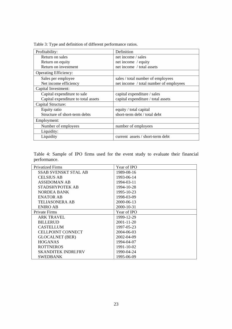
Table 3: Type and definition of different performance ratios.

Profitability: Definition Return on sales Return on equity Return on investment

net income / sales net income / equity net income / total assets

Operating Efficiency: Sales per employee Net income efficiency

sales / total number of employees net income / total number of employees

Capital Investment: Capital expenditure to sale Capital expenditure to total assets

capital expenditure / sales capital expenditure / total assets

Capital Structure: Equity ratio Structure of short-term debts

equity / total capital short-term debt / total debt

Employment: Number of employees number of employees Liquidity: Liquidity current assets / short-term debt

Table 4: Sample of IPO firms used for the event study to evaluate their financial performance. Privatized Firms Year of IPO SSAB SVENSKT STAL AB CELSIUS AB ASSIDOMAN AB STADSHYPOTEK AB NORDEA BANK ENATOR AB TELIASONERA AB ENIRO AB

1989-08-16 1993-06-14 1994-03-11 1994-10-28 1995-10-23 1998-03-09 2000-06-13 2000-10-31

Private Firms Year of IPO ARK TRAVEL BILLERUD CASTELLUM CELLPOINT CONNECT GLOCALNET (BER) HOGANAS ROTTNEROS SKANDITEK INDRI.FRV SWEDBANK

1999-12-29 2001-11-20 1997-05-23 2004-06-03 2002-04-09 1994-04-07 1991-10-02 1990-04-24 1995-06-09

23

Table 5a: Consequences of privatization. TYPE of performance indicator \ year -2 -1 1 2 Profitability: Return on sales -5.83 -5.65 -4.95 -6.22 Return on equity -5.82 -5.62 -4.86 -6.16 Return on assets -5.82 -5.69 -4.98 -6.25 Operating Efficiency: Sales per employee 5613.45 5542.75 4777.44 4190.94 Net income efficiency -46.17 89.62 262.59 307.11 Capital Investment: Capital expenditure to sale -5.75 -5.66 -4.99 -6.21 Capital expenditure to total assets -5.77 -5.67 -5.00 -6.23 Capital Structure: Equity ratio -5.26 -5.12 -4.40 -5.79 Structure of short-term debts -5.51 -5.32 -4.67 -6.00 Employment: Number of employees 11315.16 10633.58 10854.35 7721.52 Liquidity: Liquidity 54.03 -2.80 9.13 9.43 Table 5b: Consequences of privatization. TYPE of performance\ period DESCRIPTION

Profitability: Average Before Privatization

Average After Privatization

Return on sales net income / sales -5.7381 -5.5861 Return on equity net income / equity -5.7223 -5.5143 Return on assets net income / total assets -5.7557 -5.6148 Operating Efficiency:

Sales per employee sales/total number of employees 5578.0980 4484.1878

Net income efficiency net income /tot nr of employees 21.7271 284.8498

Capital Investment: Capital expenditure to sale capital expenditure/ sales -5.7058 -5.5999 Capital exp. to total assets capital expenditure/ total assets -5.7201 -5.6152 Capital Structure: Equity ratio equity / total capital -5.1895 -5.0969 Structure of short-term debts short-term debt / total debt -5.4147 -5.3353 Employment: Number of employees number of employees 10974.3700 9287.9340 Liquidity:

24

Liquidity Current assets / short-term debt 25.6161 9.2827 Table 6: Wilcoxon Signed Rank Test of median = 0.0000 versus median not = 0.0000.

Wilcoxon Estimated N Statistic Prob Median Return on sales 40 6.0 0.000 -5.291 Return on equity 40 6.0 0.000 -5.334 Return on assets 40 6.0 0.000 -5.309 Sales per employee 40 785.0 0.000 1246.000 Net income efficiency 40 703.0 0.000 80.540 Capital expenditure to sale 40 6.0 0.000 -5.282 Capital exp. to total as 40 6.0 0.000 -5.282 Equity ratio 40 25.0 0.000 -4.832 Structure of short-term debts 40 14.0 0.000 -5.121 Number of employees 40 811.0 0.000 8863.000 Liquidity 40 327.0 0.267 -1.151 Table 7: Descriptive Statistics for private firms from Sweden.

Descriptive Statistics: Variable and period Mean SE Mean Std Dev Median AAR 200 Days-Swedish Private -0.0040 0.1290 1.8300 -0.0720 CAAR 200 Days-Swedish Private -0.5570 0.3890 5.496 0 -0.6140 AAR 400 Days-Swedish Private 0.0024 0.0823 1.6459 -0.0633 CAAR 400 Days-Swedish Private -2.1680 0.2410 4.8280 -2.5410 AAR 750 Days-Swedish Private -0.0059 0.0520 1.4245 -0.0720 CAAR 750 Days-Swedish Private -2.5630 0.1810 4.9500 -2.5040 Note: AAR stands for average abnormal returns and CAAR for cumulative average abnormal returns. Table 8: Descriptive Statistics for state-owned privatized firms from Sweden.

Descriptive Statistics: Variable and period Mean SE Mean Std Dev Median AAR 200 Days-Swedish Privatized 0.0473 0.0703 0.9943 0.0088 CAAR 200 Days-Swedish Privatized 2.6400 0.3620 5.1190 1.9920 AAR 400 Days-Swedish Privatized -0.0318 0.0429 0.8586 -0.0514 CAAR 400 Days-Swedish Privatized 0.6720 0.3080 6.1510 1.1520 AAR 750 Days-Swedish Privatized -0.0065 0.0292 0.7992 -0.0261 CAAR 750 Days-Swedish Privatized -4.8170 0.2920 8.0070 -5.7240 Note: AAR stands for average abnormal returns and CAAR for cumulative average abnormal returns.

25

26

Table 9: Calculated AAR t-tests for three estimated windows 200, 400 and 750 of type 1 and 2 firms.

Type 1: Private firms

T (AAR 200 Private) = (-0.0040/0.1290) = -0.4385

T (AAR 400 Private) = (0.0024/0.0823) = 0.5832

T (AAR 750 Private) = (-0.0059/0.0520) =-3.1074 Type 2: State-owned firms

T (AAR 200 Privatized) = (0.0473/0.0703) = 9.5152

T (AAR 400 Privatized) = (-0.0318/0.0429) =- 14.8252

T (AAR 750 Privatized) = (-0.0065/0.0292) =-6.0964

Note: AAR stands for average abnormal returns. snT /µ= Table 10: Test of equality of mean average abnormal returns (AAR).

AAR 200 T=(-0.0040-0.0470)/(0.1290-0.0700)=-0.8688

AAR 400 T=(-0.0024-(-0.0318))/(0.0823-0.0429)=0.8680

AAR 750 T=(-0.0059-(-0.0066))/(0.0520-0.0292)=-0.0307

2221

2121 /// nsnsT +−= µµ

2221

2121 /// nsnsT +−= µµ

2221

2121 /// nsnsT +−= µµ

27

Table 11: Calculated CAAR t-tests for three estimated windows 200, 400 and 750 of type 1 and 2 firms.

Type 1: private firms

T (CAAR 200 Private) = (-0.5570/5.4960) =- 1.4333

T (CAAR 400 Private) = (-2.1680/4.8280) = -8.9810

T (CAAR 750 Private) = (-2.5630/4.9500) = -14.1804 Type 2: state-owned firms

T (CAAR 200 Privatized) = (2.6400/5.1190) = 7.2934

T (CAAR 400 Privatized) = (0.6720/6.1510) = 2.3185

T (CAAR 750 Privatized) = (-4.8170/8.0070) = -16.4760

Notes: CAAR stands for cumulative average abnormal returns. snT /µ= Table 12: Test for equality of mean abnormal returns (CAR)

CAR 200 T=(-0.5570-2.6400)/(0.3890-0.3620)=-118.4070

CAR 400 T=(-2.1680-0.6720)/(0.2410-0.3080)=-42.3900

CAR 750 T=(-2.5630-(-4.8170))/(0.1810-0.2920)=-20.3063

2221

2121 /// nsnsT +−= µµ

2221

2121 /// nsnsT +−= µµ

2221

2121 /// nsnsT +−= µµ

28

Table 13: Descriptive Statistics GARCH for private firms from Sweden.

Descriptive Statistics: GARCH Variable and period Mean SE Mean Std Dev Median AR GARCH 200 Sweden Private 0.0110 0.1290 1.8300 -0.0570 AR GARCH 400 Sweden Private -0.0203 0.0823 1.6459 -0.0860 AR GARCH 750 Sweden Private -0.0070 0.0520 1.4245 -0.0731 CAR GARCH 200 Sweden Private -0.4240 0.3890 5.4960 -0.4810 CAR GARCH 400 Sweden Private 1.0730 0.2410 4.8280 0.7010 CAR GARCH 750 Sweden Private 0.5320 0.1810 4.9500 0.5910 Notes: AR stands for average abnormal returns, CAR for cumulative average abnormal returns and GARCH for generalized autoregressive conditional heteroskedasticity. Table 14: Descriptive Statistics GARCH for privatized firms from Sweden.

Descriptive Statistics: GARCH Variable and period Mean SE Mean Std Dev Median AR GARCH200 Sweden Privatized 0.0159 0.0703 0.9943 -0.0226 AR GARCH400 Sweden Privatized -0.0318 0.0429 0.8586 -0.0514 AR GARCH750 Sweden Privatized -0.0065 0.0292 0.7992 -0.0261 CAR GARCH 200 Sweden Privatized 1.2200 0.3620 5.1190 0.5720 CAR GARCH 400 Sweden Privatized -0.7080 0.3080 6.1510 -0.2280 CAR GARCH 750 Sweden Privatized 0.9560 0.2920 8.0070 0.0490 Notes: AR stands for average abnormal returns, CAR for cumulative average abnormal returns and GARCH for generalized autoregressive conditional heteroskedasticity.

29

Table 15: Calculated T tests for three estimated windows 200, 400 and 750 GARCH of type 1and 2 firms.

Type 1. Private firms

T (AAR GARCH 200 Private) = (-0.0110/0.1290) = -1.2059

T (AAR GARCH 400 Private) = (-0.0203/0.0823) = -4.9331

T (AAR GARCH 750 Private) = (-0.0070/0.0520) =-0.3686 Type 2: State-owned firms

T (AAR GARCH 200 Privatized) = (0.0159/0.0703) = 9.5152

T (AAR GARCH 400 Privatized) = (-0.0318/0.0429) =- 14.8252

T (AAR GARCH 750 Privatized) = (-0.0065/0.0292) =-6.0964

Notes: AAR stands for average abnormal returns and GARCH for generalized autoregressive conditional heteroskedasticity. snT /µ= Table 16: Calculated T tests for three estimated windows 200, 400 and 750 GARCH of type 1 and 2 firms.

Type 1: Private firms

T (CAAR GARCH 200 Private) = (-0.4240/5.4960) =- 1.4333

T (CAAR GARCH 400 Private) = (1.0730/4.8280) =4.4449

T (CAAR GARCH 750 Private) = (0.5320/4.9500) = 2.9434 Type 2: State-owned firms

T (CAAR GARCH 200 Privatized) = (1.220/5.1190) = 3.3704

T (CAAR GARCH 400 Privatized) = (-0.7080/6.1510) = -2.3021

T (CAAR GARCH 750 Privatized) = (0.9560/8.007) = 3.2699

Notes: CAAR stands for cumulative average abnormal returns and GARCH for generalized autoregressive conditional heteroskedasticity.

30

Table 17: Mean AR equality test (GARCH)

AR GARCH 200 T=(0.0110-0.0159)/(0.1290-0.0703)=-0.0834

AR GARCH 400 T=(-0.0203-(-0.0318))/(0.0823-0.0429)=0.2918

AR GARCH 750 T=(-0.0070-(-0.0065))/(0.0520-0.0292)=-0.0219

2221

2121 /// nsnsT +−= µµ

2221

2121 /// nsnsT +−= µµ

2221

2121 /// nsnsT +−= µµ

Notes: AR stands for abnormal returns and GARCH for generalized autoregressive conditional heteroskedasticity Table 18: Mean CAR equality test (GARCH)

CAR GARCH 200 T=(-0.4240-1.2200)/(0.3890-0.3620)=-60.8889

CAR GARCH 400 T=(1.0730-(-0.7080))/(0.2410-0.3080)=-26.5821

CAR GARCH 750 T=(0.5320-0.9560)/(0.1810-0.2920)=3.8198

2221

2121 /// nsnsT +−= µµ

2221

2121 /// nsnsT +−= µµ

2221

2121 /// nsnsT +−= µµ

Notes: AR stands for abnormal returns and GARCH for generalized autoregressive conditional heteroskedasticity

31