the financial crisis and the changing dynamics of the … financial crisis and the changing dynamics...

BIS Papers No 65 257

The financial crisis and the changing dynamics of the yield curve1

Morten L Bech2 and Yvan Lengwiler3

Abstract

We present evidence on the changing dynamics of the yield curve from 1998 to 2011. We identify four different phases. As expected, the financial crisis represents a period of elevated yield volatility, but it can be split into two distinct periods. The split occurs when the Federal Reserve reached the zero lower bound. This bound suppressed volatility in the short end of the yield curve while increasing volatility in the long end – despite lower overall volatility in financial markets. In line with previous studies, we find that announcements with regard to the Federal Reserve’s large scale asset purchases reduce longer term yields. We also quantify the effect of widely observed economic news, such as the non-farm payrolls and other items, on the yield curve.

Keywords: Term structure of interest rates, financial crisis, interest rate dynamics, LSAP, unconventional monetary policy

JEL classification: E43, E52

1 We thank Torsten Ehlers, Jacob Gyntelberg and Peter Kugler for helpful discussions and we thank Andrew

Filardo for his useful comments. The views expressed in this paper are those of the authors and do not necessarily reflect those of the Bank for International Settlements.

2 Bank for International Settlements. 3 Dept. of Economics, University of Basel, Peter Merian-Weg 6, P.O. Box, CH–4002 Basel, Switzerland.

Corresponding author. Email addresses: [email protected] (Morten L. Bech), [email protected] (Yvan Lengwiler).

258 BIS Papers No 65

1. Introduction

The yield curve on U.S. Treasury securities is one of the most closely watched data of the global economy. Understanding its dynamics is a preoccupation of many financial market participants as well as academics. In this paper, we investigate how the dynamics of the yield curve were affected by the financial crisis and the subsequent policy responses using the “intelligible factors” framework of Lengwiler and Lenz (2010).

We identify four different phases of yield curve dynamics since 1998 (Section 3). After a “normal” phase ending mid-2004 we observe a period that is characterized by a conspicuous absence of volatility in yields. This “moderation” phase ends with the beginning of the financial crisis in August 2007. The first part of the crisis, which we label “liquidity crisis”, was characterized by money market turmoil and liquidity problems. Accordingly, we observe huge volatility in the short and medium maturity spectrum of the yield curve. This pattern abruptly changes in December 2008, after the Federal Reserve reached the zero lower bound. Since then, we observe a lack of perturbations at short maturities, but unusually large volatility in the long maturity spectrum of the yield curve. Reaching the zero lower bound appears in our analysis to be a significant event that has quantitatively changed the dynamics of the yield curve.

Our second result (Section 4) concerns the identification of the most important shocks. We quantify and locate in the maturity spectrum the most significant shocks, e.g. 9/11, the Lehman collapse, the rescue of AIG, or the increase of the large scale asset purchases (LSAPs) in March 2009.

Our third result (Section 5) concerns the measurement of the effect of surprises in key macroeconomic data on the yield curve. In particular, we measure how deviations of published indicators, such as non-farm payrolls, jobless claims, and other items, from expected values affect the yield curve over the whole maturity spectrum. We find that these surprises do indeed correlate with yield curve shocks, but the connection has become weaker in the crisis.

2. Intelligible factors

We use the decomposition of the term structure into “intelligible factors” developed by Lengwiler and Lenz (2010). We have M maturities that we observe on T days. Let tr m

denote the interest rate for a zero bond at time t which matures at time t m . The cross section of interest rates is described by three factors,

1 1, 2 2, 3 3,t t t t tr m k m k m k m m , (1)

where 3 matrixk M are the loadings and 3 matrixT are time-varying factors.

and k are constructed together so that they have certain desirable properties. Firstly, constraints are imposed on the loadings k , such that they load on different parts of the maturity spectrum, as can be seen from Figure 1. The first factor is the only one that loads on the very long end of the maturity spectrum, so we call 1 the long factor. The second factor is

the only one that loads on the very short end of the maturity spectrum, so we call 2 the short factor. The third factor has zero loading at the short and the long end of the maturity


spectrum, but it is normalized in such a way that it achieves unit loading somewhere in the middle. We call this the curvature factor.4

Secondly, the dynamics of the factors Á is described by a vector auto-regression (VAR),

0 1 1 ...t t p t p tD D D u , (2)

where 1, 2, 3,, , 't t t t and 0,..., pD D are the coefficient matrices of the VAR. We set p large

enough so that the factor innovations tu become serially uncorrelated. As described in

Lengwiler and Lenz (2010), the shape of the loadings k is adjusted in such a way that the factor innovations u are also uncorrelated with each other. As a result, the covariance matrix of the innovations, 'E uu , is diagonal, and the VAR is structural in that sense.

Figure 1

Loadings of the three factors

4 Note that these loadings differ from the more common loadings “level”, “slope”, and “curvature”, which

have become custom in applications of principal component analysis (Litterman and Scheinkman, 1991) or in the specification of Nelson and Siegel (1987).


The result of this procedure is a set of loadings that describe the long end, the short end, and the curvature of the yield curve. The dynamics of these factors are described by a structural VAR model.

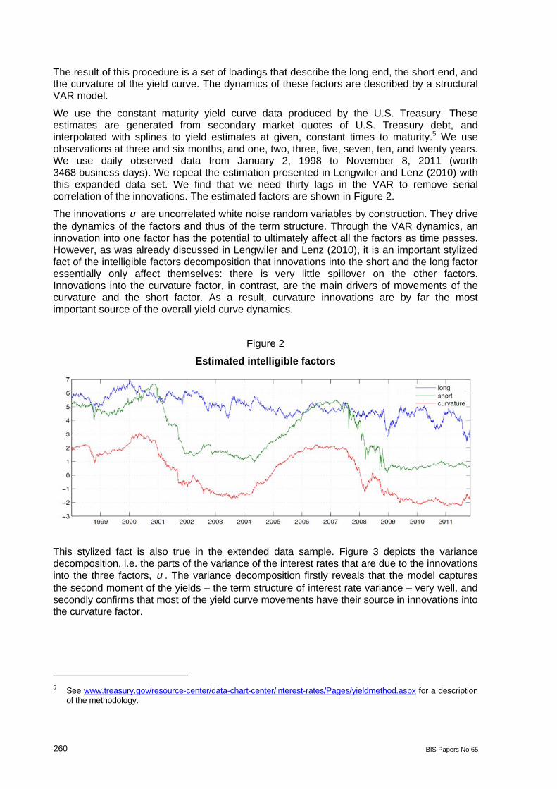
We use the constant maturity yield curve data produced by the U.S. Treasury. These estimates are generated from secondary market quotes of U.S. Treasury debt, and interpolated with splines to yield estimates at given, constant times to maturity.5 We use observations at three and six months, and one, two, three, five, seven, ten, and twenty years. We use daily observed data from January 2, 1998 to November 8, 2011 (worth 3468 business days). We repeat the estimation presented in Lengwiler and Lenz (2010) with this expanded data set. We find that we need thirty lags in the VAR to remove serial correlation of the innovations. The estimated factors are shown in Figure 2.

The innovations u are uncorrelated white noise random variables by construction. They drive the dynamics of the factors and thus of the term structure. Through the VAR dynamics, an innovation into one factor has the potential to ultimately affect all the factors as time passes. However, as was already discussed in Lengwiler and Lenz (2010), it is an important stylized fact of the intelligible factors decomposition that innovations into the short and the long factor essentially only affect themselves: there is very little spillover on the other factors. Innovations into the curvature factor, in contrast, are the main drivers of movements of the curvature and the short factor. As a result, curvature innovations are by far the most important source of the overall yield curve dynamics.

Figure 2

Estimated intelligible factors

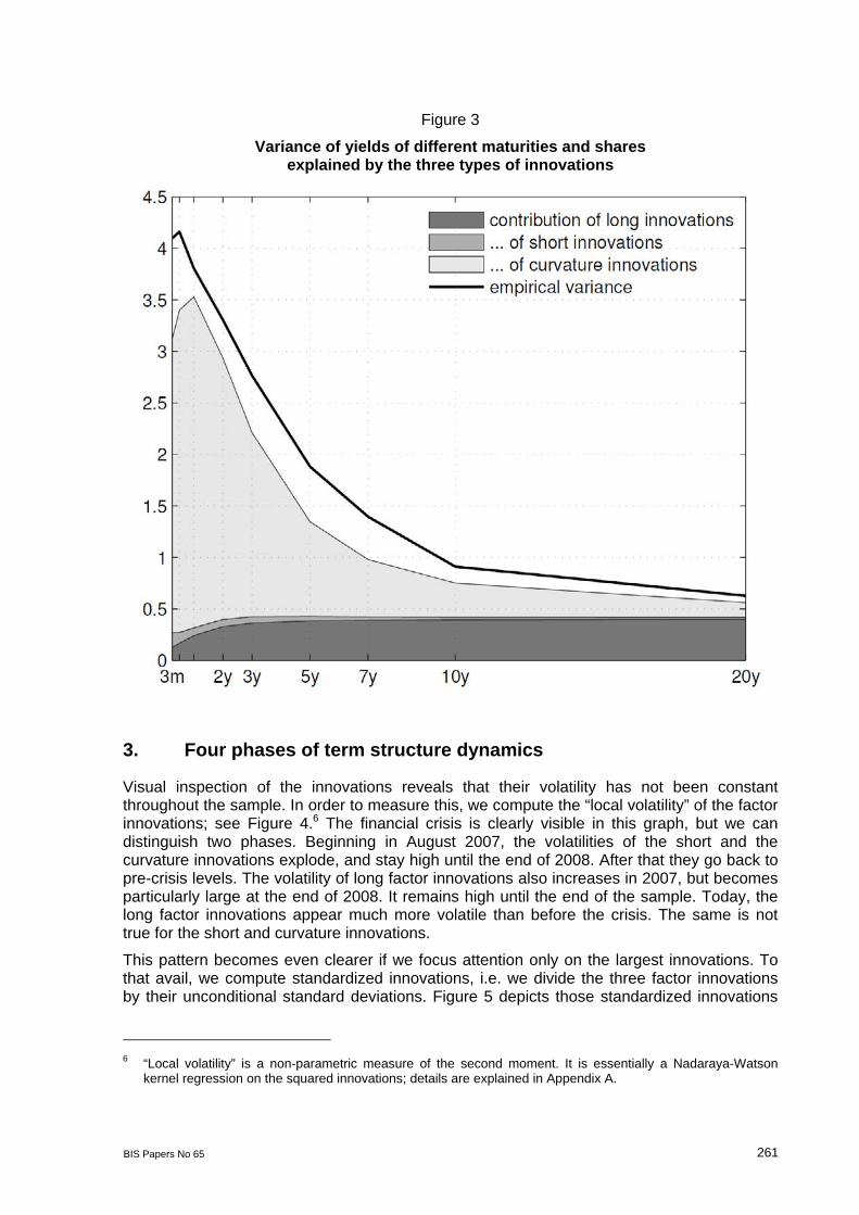
This stylized fact is also true in the extended data sample. Figure 3 depicts the variance decomposition, i.e. the parts of the variance of the interest rates that are due to the innovations into the three factors, u . The variance decomposition firstly reveals that the model captures the second moment of the yields – the term structure of interest rate variance – very well, and secondly confirms that most of the yield curve movements have their source in innovations into the curvature factor.

5 See www.treasury.gov/resource-center/data-chart-center/interest-rates/Pages/yieldmethod.aspx for a description

of the methodology.


Figure 3

Variance of yields of different maturities and shares explained by the three types of innovations

3. Four phases of term structure dynamics

Visual inspection of the innovations reveals that their volatility has not been constant throughout the sample. In order to measure this, we compute the “local volatility” of the factor innovations; see Figure 4.6 The financial crisis is clearly visible in this graph, but we can distinguish two phases. Beginning in August 2007, the volatilities of the short and the curvature innovations explode, and stay high until the end of 2008. After that they go back to pre-crisis levels. The volatility of long factor innovations also increases in 2007, but becomes particularly large at the end of 2008. It remains high until the end of the sample. Today, the long factor innovations appear much more volatile than before the crisis. The same is not true for the short and curvature innovations.

This pattern becomes even clearer if we focus attention only on the largest innovations. To that avail, we compute standardized innovations, i.e. we divide the three factor innovations by their unconditional standard deviations. Figure 5 depicts those standardized innovations

6 “Local volatility” is a non-parametric measure of the second moment. It is essentially a Nadaraya-Watson

kernel regression on the squared innovations; details are explained in Appendix A.


that are significantly different from zero at 95% confidence (so greater than 1.96 in absolute terms). We can distinguish four phases.

The first phase begins at the start of our sample and ends roughly at mid-2004 (we chose end of July). In this phase we see approximately what we would expect to see. In fact, the three standardized innovations are independent and serially uncorrelated random variables with unit variance. If they are normally distributed, for each individual series, 5% of the observations should be significantly different from zero. During this first phase, this is more or less what we observe: 3.7% of the long innovations, 2.6% of the short innovations, and 4.7% of the curvature innovations are significantly different from zero. One might label this period the “normal phase”.

The second phase begins August 2004 and ends August 2007. We call this the “moderation phase”. The exact timing between the normal and the moderation phase is difficult to pinpoint. The end of the moderation phase, however, is connected to an important event, namely BNP Paribas’s announcement that it was freezing three funds invested in sub-prime securities, which is commonly taken to mark the beginning of the financial crisis. This second phase is characterized by the marked absence of large innovations. Only 0.7% and 0.5% of the innovations into the long and the short factor are significantly different from zero. For the curvature, the number is 1.3%. Thus, this phase has very low volatility, and thus the standardized innovations turn out to be small and statistically insignificant.

This has dramatically changed with the financial crisis, which we can split into two separate phases. Phase number three, which we call the “liquidity crisis phase”, begins on August 9, 2007 and ends on December 16, 2008. This is the date when the Federal Open Market Committee lowered the target for the effective federal funds rate to a 0 to 25 basis points (bps) range and effectively reached the zero lower bound. This phase was characterized by the freezing of the interbank money market and substantial liquidity interventions by the Federal Reserve; in particular later in the period. Accordingly, we observe 23.4% of the innovations into the short factor that are significantly different from zero. For curvature, the number is also very large, 19.5%. Long factor innovations are also more volatile than before, but to a lesser extent: 8.9% of the days feature a long factor innovation that is significantly different from zero in this phase.

The fourth, the “zero lower bound phase”, begins after the Federal Reserve has reached the zero lower bound and lasts to the end of the sample. With no room downward on the federal funds rate, and traditional instruments of monetary policy exhausted, the volatility in the short and the curvature innovations vanishes. Only 0.3% and 2.5% of the innovations of these factors are significant. In contrast, 12.2% of the long factor innovations are now significantly different from zero.

We ran breakpoint tests (Bai and Perron, 1998, 2003) for the long, short, and curvature innovations, respectively. The tests for the short and the curvature innovations both find a break in early August 2007. All tests find a break in late 2008, but the dates differ. For the long innovations a third break is found in late 2009. For the period before the financial crisis, no consistent breaks are found across the three series.


Figure 4

Innovations and local volatilities In basis points


Figure 5

Large innovations into the long, short, and curvature factors, measured in multiples of unconditional standard deviations


Table 1 reports similar information to Figure 5 but focuses on the joint distribution of the innovations across days. Counting just significant or non-significant innovations, eight combinations are possible on any given day. The most likely possibility is that none of the innovations is significant. Theoretically, that should happen with probability 30.95 =86% . The long innovation should be significant while the short and the curvature innovations are not with probability 20.05 0.95 =4.5% , etc. The least likely case is that all three innovations are

significant on the same day. This event should be observed only in 30.05 0.01% of the days. The theoretical values for the cases with at least one significant innovation are reported in the first column of Table 1. The remaining columns contrast this with the actual measurement in the four phases. We observe more or less what we should observe if the shocks are independently and normally distributed in the “normal phase”. In the “great moderation phase” there are clearly too few significant innovations. In the “liquidity crisis phase” we observe way too many short and curvature innovations. In particular, we also find nineteen days where we observe significant contemporaneous short and curvature innovations. Theory would have predicted zero or one such day. There are even five days where all three innovations are significant. In the “zero lower bound phase”, finally, significant short innovations have completely vanished and significant curvature innovations are far below the theoretical expectation. Instead, there is a large density of significant long factor innovations.

Table 1

Significant shocks to the yield curve during the four phases

Theoretical normal phase

great moderation

liquidity crisis

zero lower bound

# cases share # cases share # cases share # cases share

long only 4.51% 49 2.98% 5 0.66% 144 14% 77 10.6%

short only 4.51% 30 1.82% 4 0.53% 50 14.8% 0 0.00%

curv only 4.51% 57 3.46% 10 1.32% 36 10.7% 4 0.55%

long & short only 0.24% 1 0.06% 0 0.00% 5 1.48% 0 0.00%

long & curv only 0.24% 9 0.55% 0 0.00% 6 1.78% 12 1.65%

short & curv only 0.24% 10 0.61% 0 0.00% 19 5.62% 2 0.27%

all three 0.01% 2 0.12% 0 0.00% 5 1.48% 0 0.00%

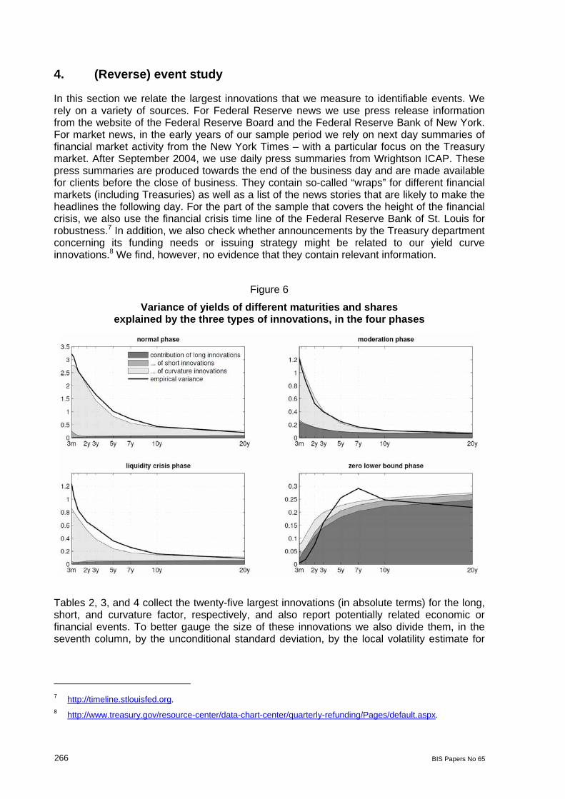
The shift of the location of the innovations during the financial crisis, and in particular to the longer part of the maturity spectrum when the zero lower bound became binding, also manifests itself in the variance attribution. We compute the variance of the yields separately for the four phases; see Figure 6 and compare with Figure 3 for the whole sample. The differences are striking. First of all, the overall variance of the yields has dramatically decreased for shorter maturities in the “zero lower bound phase”. This is a direct corollary of the fact that the zero lower bound does not allow rates to decrease further, and the Federal Reserve has not allowed the short rates to increase, hence volatility in this duration spectrum has vanished. As a result, all the volatility that remains is at longer maturities. The volatilities of the ten- and twenty-year yields is more or less unchanged for the two subperiods. Yet, because no further movements at the short end are possible, and the major innovations now occur in the long factor, almost all of the term structure of yield variance can be attributed to long innovations.


4. (Reverse) event study

In this section we relate the largest innovations that we measure to identifiable events. We rely on a variety of sources. For Federal Reserve news we use press release information from the website of the Federal Reserve Board and the Federal Reserve Bank of New York. For market news, in the early years of our sample period we rely on next day summaries of financial market activity from the New York Times – with a particular focus on the Treasury market. After September 2004, we use daily press summaries from Wrightson ICAP. These press summaries are produced towards the end of the business day and are made available for clients before the close of business. They contain so-called “wraps” for different financial markets (including Treasuries) as well as a list of the news stories that are likely to make the headlines the following day. For the part of the sample that covers the height of the financial crisis, we also use the financial crisis time line of the Federal Reserve Bank of St. Louis for robustness.7 In addition, we also check whether announcements by the Treasury department concerning its funding needs or issuing strategy might be related to our yield curve innovations.8 We find, however, no evidence that they contain relevant information.

Figure 6

Variance of yields of different maturities and shares explained by the three types of innovations, in the four phases

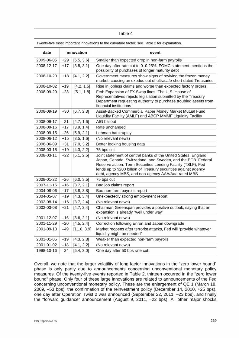
Tables 2, 3, and 4 collect the twenty-five largest innovations (in absolute terms) for the long, short, and curvature factor, respectively, and also report potentially related economic or financial events. To better gauge the size of these innovations we also divide them, in the seventh column, by the unconditional standard deviation, by the local volatility estimate for

7 http://timeline.stlouisfed.org. 8 http://www.treasury.gov/resource-center/data-chart-center/quarterly-refunding/Pages/default.aspx.


that day (the eighth column) and the conditional GARCH volatility estimate (the ninth column). We also report simple first differences of some key interest rates.

Some dates are particularly noteworthy. We measure a –37 bps shock in the short and a –49 bps shock in the curvature factor on the day the markets reopened after the 9/11 attacks. These are 5.6 and 11.0 standard deviation events, respectively. The greatest short factor innovation, however, is measured the day of the AIG bailout (–88 bps).

The Lehman bankruptcy on September 15, 2008 shows up as a large innovation in all three factors simultaneously: we measure innovations into the long factor (–23 bps), the short factor (–32 bps), and the curvature (–26 bps) on that day. This amounts to shocks between 3.5 and 5.9 standard deviations of the respective innovation series.

Notable is also the (perverse) effect of the S&P downgrade of U.S. government debt on August 8, 2011. On that day we measure a large negative innovation in the long factor (–25 bps). A possible interpretation might be that the downgrade has produced a flight for safety (“Europe will be next”) and thus increased the demand for U.S. debt.

Table 2

Twenty-five most important innovations to the long factor. The second column reports the size of the innovation in basis points (bps), and, in parentheses, relative to the unconditional and the local volatility of that day, respectively. For instance, the largest absolute long innovation is measured on March 18, 2009. We measure a –53 bps shock. This is 8.0 times the unconditional standard deviation of the long innovation series, and it is 12.3 times larger than the local volatility of that day.

date innovation event 2011-10-31 –22 [3.4, 2.0] Greek PM Papandreou announces referendum on Eurozone debt

deal 2011-10-27 +23 [3.4, 2.1] Euro summit on Greek debt 2011-09-22 –23 [3.4, 2.1] One day after Operation Twist 2 was announced 2011-08-24 +21 [3.2, 1.9] French government unveils a EUR 12 billion deficit cutting

package 2011-08-11 +25 [3.7, 2.2] Bad bond auction three days after downgrade and two days after

Fed’s forward guidance 2011-08-09 –22 [3.3, 1.9] “Forward guidance”: Low federal funds rate through mid-2013 2011-08-08 –25 [3.9, 2.3] Downgrade of U.S. government debt by S&P 2010-12-14 +25 [3.7, 2.5] Confirmation of reinvestment policy and purchase of $600 billion

of longer term Treasuries; little likelihood of increase of QE 2 2010-12-07 +23 [3.5, 2.3] (No relevant news) 2009-06-01 +30 [4.6, 2.8] Surprisingly strong data sapped the safe-haven appeal of

government debt 2009-05-27 +24 [3.6, 2.2] Concerns about the growing supply of bonds 2009-03-18 –53 [8.0, 4.3] QE 1 enlargement: Additional $750 billion agency MBS and

$100 billion agency debt; $300 in longer term Treasuries 2009-02-17 –29 [4.3, 2.3] Worries about European banks spurred investors to seek safety in

U.S. government debt 2008-12-01 –25 [3.7, 2.1] Bernanke: Fed could purchase Treasuries 2008-11-25 –27 [4.0, 2.3] QE 1: Initial large scale asset purchase announcement:

$500 billion agency MBS and $100 billion agency debt 2008-11-20 –26 [4.0, 2.3] Jobless claims reach new record 2008-09-15 –23 [3.5, 2.8] Lehman bankruptcy 2004-04-02 +25 [3.7, 3.9] (No relevant news) 2003-01-02 +26 [3.9, 3.8] (No relevant news) 2002-11-07 –22 [3.4, 2.7] One day after 50 bps cut 2001-12-07 +25 [3.7, 2.8] (No relevant news) 2001-11-15 +22 [3.3, 2.5] Dimmed hopes for further rate cuts due to positive news 2001-01-03 +27 [4.1, 4.0] 50 bps cut 1998-10-09 +23 [3.5, 2.8] (No relevant news) 1998-10-08 +25 [3.8, 3.1] Rumors of unwinding of a carry trade by a hedge fund


Table 3

Twenty-five most important innovations to the short factor; see Table 2 for explanation.

date innovation event

2008-10-20 +46 [6.9, 2.2] Government measures show signs of reviving the frozen money market, causing an exodus out of ultrasafe short-dated Treasuries

2008-10-16 +32 [4.8, 1.4] (No relevant news)

2008-10-10 –35 [5.3, 1.6] Early close ahead of Columbus day. Flight to safe haven

2008-09-23 –43 [6.5, 1.2] Bernanke supports TARP

2008-09-19 +78 [11.8, 1.8] Asset-Backed Commercial Paper Money Market Mutual Fund Liquidity Facility (AMLF) and ABCP MMMF Liquidity Facility

2008-09-17 –88 [13.3, 2.1] AIG bailout

2008-09-15 –32 [4.8, 0.8] Lehman bankruptcy

2008-03-24 +57 [8.7, 2.3] FRBNY announces that it will provide term financing to facilitate JPMorgan Chase’s acquisition of Bear Stearns

2008-03-19 –31 [4.7, 1.3] One day after 75 bps cut. Reduction of required capital for Fannie Mae and Freddie Mac

2008-03-18 –36 [5.5, 1.5] 75 bps cut

2008-01-22 –49 [7.4, 2.4] 75 bps cut

2007-12-24 +36 [5.5, 2.2] (No relevant news)

2007-09-04 +51 [7.7, 2.1] Money market turmoil

2007-08-29 –36 [5.4, 1.1] Money market turmoil




2007-08-20 –70 [10.6, 1.9] Money market turmoil

2007-08-15 –49 [7.4, 1.5] Money market turmoil after BNP Paribas writedown

2001-09-13 –37 [5.6, 2.2] Market reopens after terrorist attacks, Fed will “provide whatever liquidity might be needed”

2000-12-26 +69 [10.5, 2.2] (No relevant news)

2000-12-21 –43 [6.6, 1.6] Speculation that Federal Reserve may lower interest rates before scheduled meeting at the end of January

1998-10-19 +40 [6.1, 1.8] Two days (!) after 50 bps rate cut, reversing move of short factor a day earlier

1998-10-16 –49 [7.4, 2.0] One day after 50 bps rate cut

1998-10-08 –31 [4.8, 1.9] Rumors of unwinding of a carry trade by a hedge fund


Table 4

Twenty-five most important innovations to the curvature factor; see Table 2 for explanation.

date innovation event

2009-06-05 +29 [6.5, 3.6] Smaller than expected drop in non-farm payrolls

2008-12-17 +17 [3.8, 3.1] One day after rate cut to 0–0.25%. FOMC statement mentions the possibility of purchases of longer maturity debt

2008-10-20 +18 [4.1, 2.2] Government measures show signs of reviving the frozen money market, causing an exodus out of ultrasafe short-dated Treasuries

2008-10-02 –19 [4.2, 1.5] Rise in jobless claims and worse than expected factory orders

2008-09-29 –23 [5.1, 1.8] Fed: Expansion of FX Swap lines. The U.S. House of Representatives rejects legislation submitted by the Treasury Department requesting authority to purchase troubled assets from financial institutions

2008-09-19 +30 [6.7, 2.3] Asset-Backed Commercial Paper Money Market Mutual Fund Liquidity Facility (AMLF) and ABCP MMMF Liquidity Facility

2008-09-17 –21 [4.7, 1.6] AIG bailout

2008-09-16 +17 [3.9, 1.4] Rate unchanged

2008-09-15 –26 [5.9, 2.1] Lehman bankruptcy

2008-06-12 +15 [3.5, 1.6] (No relevant news)

2008-06-09 +31 [7.0, 3.2] Better looking housing data

2008-03-18 +19 [4.3, 2.2] 75 bps cut

2008-03-11 +22 [5.1, 2.5] Joint statement of central banks of the United States, England, Japan, Canada, Switzerland, and Sweden, and the ECB. Federal Reserve action: Term Securities Lending Facility (TSLF), Fed lends up to $200 billion of Treasury securities against agency debt, agency MBS, and non-agency AAA/Aaa-rated MBS

2008-01-22 –26 [6.0, 3.5] 75 bps cut

2007-11-15 –16 [3.7, 2.1] Bad job claims report

2004-08-06 –17 [3.8, 3.8] Bad non-farm payrolls report

2004-05-07 +19 [4.3, 3.4] Unexpectedly strong employment report

2002-08-14 +16 [3.7, 2.4] (No relevant news)

2002-03-08 +21 [4.7, 3.4] Chairman Greenspan provides a positive outlook, saying that an expansion is already “well under way”

2001-12-07 –16 [3.6, 2.1] (No relevant news)

2001-11-29 –20 [4.5, 2.4] Correction following Enron and Japan downgrade

2001-09-13 –49 [11.0, 3.9] Market reopens after terrorist attacks, Fed will “provide whatever liquidity might be needed”

2001-01-05 –19 [4.3, 2.3] Weaker than expected non-farm payrolls

2001-01-02 –18 [4.1, 2.2] (No relevant news)

1998-10-16 –24 [5.4, 3.0] One day after 50 bps rate cut

Overall, we note that the larger volatility of long factor innovations in the “zero lower bound” phase is only partly due to announcements concerning unconventional monetary policy measures. Of the twenty-five events reported in Table 2, thirteen occurred in the “zero lower bound” phase. Only four of these large innovations are related to announcements of the Fed concerning unconventional monetary policy. These are the enlargement of QE 1 (March 18, 2009, –53 bps), the confirmation of the reinvestment policy (December 14, 2010, +25 bps), one day after Operation Twist 2 was announced (September 22, 2011, –23 bps), and finally the “forward guidance” announcement (August 9, 2011, –22 bps). All other major shocks


were due to business cycle surprises or are related to the crisis of the European currency union. This point is nicely illustrated in Figure 7.

Figure 7

Major long factor innovations in the zero lower bound phase. The last five months of the sample are depicted separately in the right-hand panel because there is more action there.

5. News

It is well-documented that economic news releases and in particular surprises from market expectations move Treasury yields (see e.g. Fleming and Remolona, 1999). Not surprisingly, a similar relationship holds for our factors. A natural question is whether or not the changing dynamics of the yield curve can (in part) be explained by changing dynamics in terms of economic news surprises. Table 5 shows the results of regressing innovations into our long, short, and curvature factors on day-of-release surprises for a range of economic indicators. The indicators we consider include the Conference Board Consumer Confidence Index®, the Institute for Supply Management (ISM) purchasing managers index (PMI), the advance GDP print, the unemployment rate, industrial production, retail sales, housing starts, one-family houses sold, the personal consumption expenditure price index, capacity utilization, initial jobless claims, the leading economic indicator index, and the federal funds rate target. We measure surprises as the difference between the actual value released and the median value from an “expectations” survey among Wall Street economists conducted by Bloomberg News prior to the release. To put the surprises on a common scale we standardized them by their standard deviation over the sample. Moreover, we switch the sign of some surprise variables, so that a positive surprise is “good news”. For instance, non-farm payroll surprises are measured as actual release minus median expectation, whereas jobless claims are defined the other way around. In addition, we control for non-linear effects by including the squared standardized surprises as additional regressors.

Besides the results for the entire sample, we also split our sample in two with a view to investigating whether or not the impact of economic news has changed with the financial crisis. Our “pre-crisis” sample runs from 1998 to August 8, 2007 (“normal” and “great moderation” phases) and the “crisis” sample covers the remainder of our sample (“liquidity


crisis” and “zero lower bound” phases). Furthermore, because our left-hand variables exhibit clustered volatility (see Section 3 and Figure 4 in particular), we use the EGARCH specification. In order to capture general market volatility we add the VIX as an exogenous variable to the variance equation. We also add dummies for our phases that we identified in Section 3 to the variance equation.

Consistent with previous literature we find that the non-farm payrolls are among the most informative signals. This was the case before the crisis, and has remained so: non-farm payroll surprises (linear and squared) have highly significant effects on all three yield curve factors. PMI surprises used to be significant predictors of all three innovations before the crisis; since the crisis they contain information only on long innovations. Surprises about retail sales and about capacity utilization used to contain information on long and curvature innovations before the crisis; in the crisis, retail sales surprises seem to no longer affect the curvature, and capacity utilization has lost its connection to the yield curve completely. Surprises about jobless claims used to affect curvature innovations before the crisis, but now affect long innovations instead. Surprises concerning the FOMC’s federal funds target rate used to be highly significant with respect to short factor innovations; they have lost their explanatory power during the crisis. Prior to the financial crisis, our economic surprise indicators could account for 4.5%, 1.5%, and 6.6% of the variation in the long, short, and curvature factors (as measured by the R2-statistic). In our crisis sample, the comparable numbers are 3.2%, 0.3%, and 0.9%.

The phase dummies in the variance equation partially verify our partition of the sample into four phases. Interestingly, the “great moderation” dummy is not significant. The general reduction of the volatility of our innovations between 1998 and the beginning of the financial crisis seems fully captured by the VIX. The two other phase dummies, however, come in as significant, as expected. The “liquidity crisis” dummy measures a higher volatility for short and curvature innovations, but is not significant in the variance equation of the long innovations. The “zero lower bound” dummy, on the other hand, measures a significantly higher volatility of long factor innovations, but significantly lower volatility of the short factor innovations. With respect to curvature innovations, this coefficient is either negative (pointing to a reduced volatility of curvature shocks in this phase) or statistically insignificant.

6. Conclusions

The financial crisis has deeply affected financial markets as well as the economy as a whole. This has also affected the yield curve and its dynamics. We document these changes in this paper. Our main results can be summarized as follows: Firstly, we divide the dynamics of the yield curve into four phases. The first two phases occur prior to the financial crisis. The second phase is characterized by substantially less volatility of the yields compared to the first phase. However, this is well explained by the simultaneous decline of overall financial market volatility during that period as measured by the VIX.

The third and the fourth phase comprise the financial crisis. This means that we can divide the crisis into two distinct subperiods. In the first subperiod, the yield curve experienced very strong shocks in the short and medium maturity spectrum due to the freezing of the money market and subsequent emergency measures taken by the Federal Reserve. The second part of the financial crisis began when the federal funds rate reached the zero lower bound. From that point forward, we find an absence of shocks hitting the yield curve at low and medium maturities. Instead, the longer end of the curve experiences greater disturbances than before.

Secondly, we perform a (reverse) event study in which we match the greatest shocks to the yield curve with headline news. We find that some large shocks are associated with


announcements by the Federal Reserve. However, a significant number of shocks in particular in the recent past are due to international developments.

Thirdly, we identify and quantify the informational content of well-known macroeconomic surprise data. We find that that some, but not all of these variables have lost significance in the crisis. The overall information content of these news variables with respect to the yield curve, however, is small.

Table 5

Effects of macroeconomic news on the yield curve

variable long innovations short innovations curvature innovations

sample pre-crisis crisis all pre-crisis crisis all pre-crisis crisis all

constant –0.033 –0.090 –0.065 0.235 0.530 0.328 0.206 –0.195 0.122

standardized surprise in:

Capacity utilization 2.205** 0.813 2.186** –0.740 –0.457 –0.575 1.233** –0.224 0.808**

Consumer confidence 1.350** –0.311 1.135** –0.358 0.191 –0.135 0.449 0.224 0.360

Initial jobless claims 0.975 2.955** 1.620** –0.027 –0.160 –0.174 1.005** –0.553 0.661**

Federal funds target –2.689 –7.409 –1.334 –12.83*** –1.362 –10.40*** –0.471 3.792 –1.001

Advance GDP –0.668 –2.094 –0.809 0.018 0.697 –0.038 0.528 –0.654 0.571

One-family houses sold 0.996** 0.711 0.999** –0.129 –0.076 –0.102 –0.047 0.502 0.010

Housing starts –0.407 2.167 –0.179 –0.103 –1.067 –0.264 0.055 1.795* 0.126

Industrial production –0.990 2.364 –0.694 0.439 0.098 0.334 –0.480 0.537 –0.199

ISM PMI 1.597*** 3.136** 1.941*** –1.305*** 0.348 –0.483* 1.370*** –0.620 0.888***

LEI 0.274 0.175 0.175 –0.833 –0.287 –0.502 –0.708 –0.574 –0.754**

Non-farm payrolls 3.578*** 4.786** 3.761*** –2.009*** –2.390*** –2.206*** 3.117*** 1.938** 2.948***

PCE price index 0.356 –3.064* –0.482 –1.324* –0.351 –0.724 –0.141 –0.345 –0.124

Retail sales 1.445** 5.530*** 2.110*** –0.570 0.933 –0.143 1.176*** –1.490* 0.581*

Unemployment rate 0.783 1.477 0.961* –0.542 –0.524 –0.644** 2.065*** 0.837* 1.477***


Table 5 (cont)

Effects of macroeconomic news on the yield curve variable long innovations short innovations curvature innovations

sample pre-crisis crisis all pre-crisis crisis all pre-crisis crisis all

constant –0.033 –0.090 –0.065 0.235 0.530 0.328 0.206 –0.195 0.122

squared standardized surprise in:

Capacity utilization –0.655 –1.615 –0.968* 0.190 –0.049 0.049 –0.657* 0.809** –0.052

Consumer confidence –0.119 –1.337** –0.286 –0.391 –0.379 –0.390** –0.085 0.67** 0.133

Initial jobless claims 0.101 0.096 0.184 –0.296 0.018 –0.232* 0.197 0.024 0.149

Federal funds target –0.331 11.666 1.339 –7.455** –6.158 –6.005** 4.580 –11.21 3.450*

Advance GDP 0.715 0.118 0.681 –1.056** 0.155 –0.518 0.459 –0.468 0.455

One-family houses sold –0.090 1.541 –0.063 –0.082 –0.962 –0.137 0.083 0.463 0.047

Housing starts –0.098 –1.663 –0.143 –0.086 –0.704 –0.142 –0.174 0.323 –0.169

Industrial production 0.220 1.513 0.627 –0.180 –0.008 –0.015 0.740* –0.315 0.179

ISM PMI 0.809*** –0.025 0.626*** –0.290 –0.377 –0.354** –0.199 0.213 –0.062

LEI 0.668 0.594 0.580 0.198 0.253 0.314 0.204 –0.066 0.195

Non-farm payrolls 0.782*** 1.031 0.821*** –0.622*** –1.396*** –0.774*** 0.326** 1.989*** 0.296**

PCE price index –0.826 –0.677 –0.747 1.235* 1.079* 1.086** 0.202 0.276 0.304

Retail sales 0.223 0.078 0.102 0.023 0.135 –0.056 0.023 –0.167 0.180

Unemployment rate 0.066 0.477 0.145 0.000 0.670** 0.490** –0.456 –0.900*** –0.438**

Variance equation

constant 0.005 2.658** 0.043 –0.086** 0.284** –0.001 –0.067** 0.179 –0.046**

1 / 1 0.077*** 0.092 0.098*** 0.260*** 0.271*** 0.298*** 0.144*** 0.251*** 0.178***

1 / 1 0.013 0.034 0.012 –0.061*** –0.112*** –0.072*** –0.024 –0.003 –0.021

2log 1 0.969*** –0.022 0.952*** 0.931*** 0.887*** 0.907*** 0.965*** 0.891*** 0.956***

great moderationdummy 0.002

–0.006 –0.004 –0.039* 0.000 –0.014

liquidity crisis dummy

0.015* 0.145*** 0.051***

zero lower bound dummy

0.415** 0.026** –0.288*** –0.086*** –0.166** –0.010

VIX 0.002*** 0.043** 0.002*** 0.004*** 0.001 0.003** 0.002** 0.002 0.001**

R2 0.045 0.032 0.035 0.015 0.003 0.007 0.066 0.009 0.033

Note: *,**,*** denotes significance at the 10%, 5%, and 1% level, respectively.


Appendix A.: Spot and local volatility

This is a purely technical appendix which is not necessary to understand the economic content of the paper. It explains the concept of “local volatility” that is used in some places in the main part of the article.

We aim at quantifying the changing volatility of the innovations u . Simple visual inspection suggests heteroscedasticity. We fully acknowledge that this feature of the data is not in line with the specification of the model. After all, we assumed normally distributed homoscedastic innovations when estimating the loadings and the VAR with maximum likelihood. Taking the heteroscedasticity fully into account at the estimation stage of the model seems very challenging. Being aware of this inconsistency, here we simply aim to measure the stochastic volatility of the innovations as they present themselves from the model that was estimated assuming homoscedasticity.

Consider a continuous-time diffusion,

,t t t tdX dt dW (A.1)

where tW is a standard Brownian motion. 2t is the spot variance process, which is not

observed. Instead, we observe only tX at discrete points in time, 1 2 ... nt t t . Based on

work by Bandi and Phillips (2003), Kristensen (2010) establishes that one can estimate 2

as

1

2

112

11

ˆ ,i

ni ti h

Th ii

t iXK t X

K t

(A.2)

where hK is a kernel function with bandwidth h . This is a Nadaraya-Watson kernel regression on the squared first difference of X . Spot volatility is simply the square root of the estimated spot variance. In our application, X is one of the factor innovations in the VAR model, i.e. fu for 1,2,3f .

In order to estimate spot volatility, two choices need to be made, namely the specification of the kernel function K and the selection of the bandwidth h . To select the bandwidth, we use the cross-validation technique; that is, we minimize the mean squared “leave-one-out” residuals. The kernel function K is symmetric around zero if it weighs observations in the future the same way as observations in the past. Most popular kernel functions have this property. Symmetric kernel functions have, however, the disadvantage that for close to the edge of the sample, they assign positive weights to observations outside the available sample, which biases the estimation. This is a well-known problem in non-parametric econometrics.

One way to address this problem is to use a locally adapting kernel function. Such a function was for instance proposed by Brown and Chen (1999) and Chen (2000). Their kernel function, based on the beta-function, automatically adapts to the boundaries of the sample: for close to the first observation 1t , the kernel is right-sided, for close to the last

observation nt , the kernel is left-sided. We have experimented with this kernel but found it to give unsatisfactory estimates in our application. The volatility measure has significantly more high-frequency variability close to the edge of the sample than in the interior, which suggests that the precision of the estimate deteriorates close to the edge, or that the bandwidth becomes too small.


For this reason, we resort to an older, simpler idea that was proposed by Schuster (1991). It consists of reflecting observations close to the edge of the sample to the other side. So,

3 2 1..., , ,

n n nt t tX X X

are appended in reverse order as 1 2 3, , ,...

n n nt t tX X X

, and then the

symmetric kernel function is applied to these synthetically expanded observations. We use the popular (symmetric) Epanechnikov specification as the kernel function.

This procedure as described so far is, however, not very successful in our application. The estimated spot volatilities turn out to be much too large on average. Only about 1% of the absolute innovations are greater than 1.96 times the estimated spot volatilities. It is not completely clear why this is the case. It may be due to the fact that equation (A.1) is not the correct model for the innovations u . After all, these are residuals and they have, by construction, no drift, so 0t .9

Because the spot volatility does not appear reasonable, we compute a slightly simpler and maybe more transparent measure. We apply the Nadaraya-Watson kernel regression on the squared innovations directly instead of on the squared first differences,

2

2 1

1

i

nh i ti

Th ii

K t X

K t

. (A.3)

This is the same as the approach suggested by Carroll (1982) and Hall and Carroll (1989). They consider a model where the mean can be parametrically estimated but the variance cannot. In our case, t is zero by definition, so the setting is simpler.

Figure A.8

Curvature innovations and 50% confidence interval using local volatility estimate

We use the same kernel function and reflection technique as before and perform the cross-validation bandwidth optimization. The result is an estimate of the volatility that seems much more reasonable. We call the square root of 2

the local volatility, in order to distinguish it

9 Consider 2 2 21 1 12t t t t t tE u u E u E u E u u

. In our case, u is serially uncorrelated by

construction, so 1 0t tE u u . Consequently, the spot variance overestimates the variance of u by a factor

of two, 2 2 21 1t t t tE u u E u E u

.


from the spot volatility. The size of this volatility measure appears more appropriate: 4.7% of the absolute innovations into the long factor are greater than 1.96 times the estimated local volatility of this factor innovation. For curvature, the corresponding number is 4.8%, reasonably close to the 5% one might expect. Only for the short factor innovations do we find that only 3.3% of the innovations are in absolute terms greater than 1.96 times the estimated local volatility. Still, this is much better than the 1% we get when using spot volatility. The optimized bandwidths are 47.0 days for the long factor innovations, 9.7 days for the short factor innovations, and 23.5 days for the curvature innovations. Figure A.8 depicts, as an example, the innovations into the curvature factor, as well as a 50% confidence band using the local volatility estimate.

References

Bai, J., Perron, P., 1998. Estimating and testing linear models with multiple structural changes. Econometrica 66, 47–78.

Bai, J., Perron, P., 2003. Computation and analysis of multiple structural change models. Journal of Applied Econometrics 18, 1–22.

Bandi, F., Phillips, P., 2003. Fully nonparametric estimation of scalar diffusion models. Econometrica 71, 241–283.

Brown, B., Chen, S., 1999. Beta-Bernstein smoothing for regression curves with compact support. Scandinavian Journal of Statistics 26, 47–59.

Carroll, R., 1982. Adapting for heteroscedasticity in linear models. The Annals of Statistics 10, 1224–1233.

Chen, S., 2000. Beta kernel smoothers for regression curves. Statistica Sinica 10, 73–91.

Fleming, M., Remolona, E., 1999. Price formation and liquidity in the U.S. Treasury market: The response to public information. Journal of Finance 54, 1901–1915.

Hall, P., Carroll, R., 1989. Variance function estimation in regression: The effect of estimating the mean. Journal of the Royal Statistical Society, Series B 51, 3–14.

Kristensen, D., 2010. Nonparametric filtering of the realized spot volatility: A kernel-based approach. Econometric Theory 26, 60–93.

Lengwiler, Y., Lenz, C., 2010. Intelligible factors for the yield curve. Journal of Econometrics 157, 481–491.

Litterman, R., Scheinkman, J., 1991. Common factors affecting bond returns. The Journal of Fixed Income 1, 54–61.

Nelson, C., Siegel, A., 1987. Parsimonious modeling of yield curves. The Journal of Business 60, 473–489.

Schuster, E., 1991. Incorporating support constraints into nonparametric estimators of densities. Communications in Statistics: Theory and Methods 14, 1123–1136.

the financial crisis and the changing dynamics of the … financial crisis and the changing dynamics...

Documents