the fine structure constant and interpretations of … · ejtp 9, no. 26 (2012) 135–146...

EJTP 9, No. 26 (2012) 135–146 Electronic Journal of Theoretical Physics

The Fine Structure Constant and Interpretations ofQuantum Mechanics

Ke Xiao∗

P.O. Box 961, Manhattan Beach, CA 90267, USA

Received 10 October 2011, Accepted 7 December 2011, Published 17 January 2012

Abstract: The fine structure constant give a simple derivation of the localized wavefunction,Schrödinger equation, double-slit and the uncertainty principle in Quantum Mechanics.The wave-particle duality link to the space-time property of matter by Planck constant. Thedouble-slit formula is |ψX |2 = 2|sinc(a′kX)|2[1 + cos(akX − ωδT ′ + ϕ)], where the cross-linkedangle for double-slit, T ′1 = Tc cos (θ2) and vice versa.c© Electronic Journal of Theoretical Physics. All rights reserved.

Keywords: Fine structure constant; Wavefunction; Uncertainty Principle; Quantum MechanicsPACS (2010): 03.65.-w; 42.25.Fx; 61.05.fg

1. Introduction

The fine-structure constant α is deeply involved in the Quantum theory.[1,2] Pauli consid-ered quantum mechanics to be inconclusive without understanding of the fine structureconstant.[2] Feynman also said that nobody understands quantum mechanics.[3] There aremany controversies surrounding its reality, determinative, causality, localization and com-pleteness. Beyond the Copenhagen interpretation, other interpretations include Many-World, Hidden Variable, de Broglie-Bohm, Ensemble, von Neumann/Wigner, Quantumlogic, etc, each with its own compromises. As a new approach, here we discuss a finestructure constant interpretation of Quantum Mechanics.[4]

(1) Wavefunction and Wave-Particle DualityOne basic problem in the quantum interpretation is the wavefunction. From 1926 to

1928, there were some proposed quantum wave equations HΨ = i� ∂∂tΨ; for example

∗ Email: [email protected]

136 Electronic Journal of Theoretical Physics 9, No. 26 (2012) 135–146

[−�2

2μ∇2 − V (r)]Ψ(r, t) = i� ∂

∂tΨ(r, t) (a) Schrodinger (1)

12m

(→σ · (→p − q

→A))2 + qφ]Ψ1,2 = i� ∂

∂tΨ1,2 (b) Pauli

[∇2 − (mc�)2]Ψ(r, t) = 1

c2∂∂tΨ(r, t) (c)Klein−Gordon

[βmc2 + 3∑

k=1αkPkc]Ψ1,2,3,4 = i� ∂

∂tΨ1,2,3,4 (d)Dirac

where the non-relativistic equations are (a) for the atomic electron configuration and(b) for the Dirac limitation of spin-1/2 particles, and the other two relativistic quantumequations are (c) for the spin-0 free particle and (d) for the spin-1/2 particle-antiparticles.The different Hamiltonians H on the left-side were proposed based on the imitationsof various classical physical processes, such as Schrodinger’s Hamiltonian imitating theoptical wave equation.

The eigenvalues of a negatively charged electron orbiting the positively charged nu-cleus are determined by the time-independent Schrödinger equation HΨ(r) = EΨ(r).[5]Wavefunction Ψnlm = Rnl (r) Ylm (θ, φ) (n, l, m are quantum numbers) is geometri-cally quantized in a 3D cavity. According to Born, Ψ is the probability amplitudeand ΨΨ∗ is the probability density.[6] Each state only allows two counter-spin electrons(ms = ±1

2) per the Pauli principle, e2 |Ψnlm|2 = α�c |Ψnlm|2 is the probability density

of the paired charge. The Schrödinger wavefunction Ψnlm indeed describes the twinsin a box. Dirac’s relativistic quantum equation solves the spin-1/2 problem. Then,e |Ψnlmms |2 =

√α�c |Ψnlmms |2 is the probability density of the charge. The fine structure

constant can be defined as the conservation of angular momentum

e2

c= ±α� (2)

The wavefunction had an entropy format S = klnΨ for HΨ = EΨ in Schrödinger’sfirst paper in 1926.[5] The Boltzmann constant k is linked to α by the dimensionless black-body radiation constant αR and primes αR = e2( 4σ

ck4)1/3 = (∏ p2

p2+1)1/3α = 0.86976680α =

1157.555

.[7] A plane wave function Ψ(r, t) and the Born probability density |Ψ(r, t)|2 are

Ψ(r, t) = Ae−i�(p·r−Et) = Ae−

i�Etψ(r) = f(t)ψ(r) (3)

|Ψ(r, t)|2 = ΨΨ∗ = [Ae−i�Etψ(r)][Ae−

i�Etψ(r)]∗

= Ae−i�Etψ(r) · Ae i

�Etψ∗(r) = A2|ψ(r)|2

The Einstein/de Broglie wave-particle duality is linked to the reciprocal space-time properties of matter.[8,9] Note that period T = 1/ν [T] and wavelength λ =

1/k [L], the property of particle-wave is defined by the spin over time-space.

E = �ω i.e. E = hν = h/T (spin/time) (4)p = �k i.e. p = hk = h/λ (spin/space)

where the conservation of angular momentum in the reduced Planck (Dirac) constanth = ET = pλ (i.e., � = E/ω = p/k), and the electron spin �/2 can only be interpretedby the 4-dimensional spacetime of the relativistic Dirac equation.[10,11]

Electronic Journal of Theoretical Physics 9, No. 26 (2012) 135–146 137

(2) Schrödinger Equation Derivation From α

We notice that e2/c in (2) has the same dimension with �, Et, and p · r. Let’s usei = −1/i, and e−iπ = −1 = i2 = lne−1 to rewrite (2) in the four-dimensional space-time{r, t} = {x, y, z, t}, i.e., link the charge to space, time, and spin

e2

c= p · r− Et = ±α� = ±i2 · α� · lne−1 = i� ln e∓iα (5)

where (p · r−Et)/� = (k · r−ωt) = k(r−ct) link to the relativity. (5) may also work forEt or p · r separately (e.g., let t ≡ 0 for the time-independent wavefunction). From (5),

lne∓iα = − i�(p · r−Et) = −i(k · r−ωt) = ´ Ψ

A

duu= ln Ψ

A(6)

In Hilbert space (eiHt/� = eiEt/�), a nonlocal plane wavefunction Ψ(r, t) = Ae−i�Etψ(r),

i.e., Ψ(r, t) = Ae−i(p·r−Et)/� is defined as the exponential (6), and the wavefunctioncan be locally quantized by the fine structure constant as (5)

Ψ(r, t) = Ae−i�(p·r−Et) = Ae∓iα = A cos(∓α)∓ iA sin(∓α) = a∓ bi (7)

In (7), obviously, Ψ(r, t) =∑anψn(r) =

∑ane

−iEt/�ψn(r) and´V|Ψ|2dV = 1. It is a

Hermitian function, where the real part is an even function and the imaginary part is anodd function. From Ψ(r, t) = Ae−

i�(p·r−Et) = Ae−

i�(Px·x+Py ·y+Pz ·z−Et),

∂∂tΨ(r, t) = − i

�EΨ(r, t) (8)

∂2

∂x2Ψ(x, t) = − 1�2P 2xΨ(x, t)

i.e., the operators can also be derived mathematically from (8)

E = i� ∂∂t; P = i�∇; P 2 = −�2∇2 (9)

The Hamiltonian H = T + V = E is the sum of kinetic and potential energy, andT = 1

2μP2. In this way, the Schrödinger equation can be derived from the fine

structure constant (2)

[−�2

2μ∇2 − V (r)]Ψ(r, t) = i� ∂

∂tΨ(r, t) (10)

−�22μ∇2 − V (r)]Ψ(r) = EΨ(r)

To solve the Schrödinger equation for the atomic electron configuration, we need toconvert Ψ(r) = Ψ(x, y, z) to Ψ(r) = Ψ(r, θ, φ). However, the quantum principle is inde-pendent of the coordinate system. The Schrödinger equation can also be mathematicallytransformed into Heisenberg matrix mechanics or Feynman path integral formulation.Therefore, the quantum principle is also independent of the mathematical expression(some confusion may be caused by usage of different symbols and terms). Althoughthere are different ways to describe Quantum theory, all theoretical physicists agree that


the fine structure constant is the magic number , and it can not be derived from theQuantum Mechanics.[1,2] From (7), Ψ(r) = e− i

�(p·r) = e−iα is for a negatively charged

electron orbiting a positively charged nucleus, which has the complex number conjugatesΨ(r) = a− bi and Ψ∗(r) = a+ bi, then ΨΨ∗ is a real number for the probability density

|Ψ|2 = ΨΨ∗ = (a− bi) (a+ bi) = a2 + b2 = 1 (11)

Specifically, if Ψ = a(1− i), then the normalization from (11) yields a = 1/√2.

After localization, the variable wavefunctions become complex numbers (vectors inHilbert space). The complex addition (vector sum) Ψ12 of Ψ1 = a+ bi and Ψ2 = c+ di is

Ψ12 = Ψ1 +Ψ2 = (a+ bi) + (c+ di) = (a+ c) + (b+ d)i (12)

A superposition f(x1 + x2 + · · · ) = f(x1) + f(x2) + · · · is interpreted as a vector sum as(12). There is an interference term when calculating the probability density from (12)

Ψ12Ψ∗12 = [(a+ c) + (b+ d)i][(a+ c)− (b+ d)i] (13)

= (a+ c)2 + (b+ d)2

= a2 + b2 + c2 + d2 + 2(ac+ bd)

or Ψ12(r, t)Ψ∗12(r, t) = a2 + b2 + c2 + d2 + 2(ac+ bd)eiEδt/�. This enlightens the physical

interpretation of wavefunction. There is a hidden fine-structure constant α in thelocalized wavefunction (7). It naturally yields the eigenvalues En = −Ee(

αn)2 from the

Schrödinger equation, where Ee = 12mec

2; the fine-structures �EF = ±Ee(αn)4[3

4− n

j+1/2]

are from Dirac’s relativistic equation, where j = l+ms is the total angular momentum.[4]In the magnetic field, QED yields the Lamb shift�EL = Ee

α5

2n3 [k(n, l)± 1π(j+1/2)(l+1/2)

] and

the hyperfine structures due to the “nuclear spin” �EH = ±Eegpβ

α4

n3

[F (F+1)−j(j+1)−I(I+1)

j(j+1)(2l+1)

],

where the total angular momentum F is equal to the total nuclear spin I plus the totalorbital angular momentum J ; the proton g-factor gp = 5.585. This gives experimentalconfirmation of a connection between α ∼= 1/137 and β ∼= 1836 . In fact, the reducedmasses μ = me·mp

me+mp= β·me

β+1≈ me always involve β in the Schrödinger equation (10).

Quantum theory not only describes the electron configurations around the nucleus, butalso considers the effect of nuclear mass. Neglecting interaction between electrons, theabove eigenvalues are linked to Eμ = 1

2μc2 = 0.25536[MeV] and αn.

En=−Eμ(αn)2 ∝ α2 = 5.3×10−5 (14)

�EF=±Eμ(αn)4[

34− nj+1/2

] ∝ α4 = 2.8×10−9�EL=Eμ

α5

2n3 [k(n,l)± 1π(j+1/2)(l+1/2)

] ∝ α5 = 2.1× 10−11

�EH=±Eμgpβ

α4

n3

[F (F+1)−j(j+1)−I(I+1)

j(j+1)(2l+1)

]∝ α4/β = 1.5×10−12

In (14), we have En > �EF > �EL > �EH since α2 > α4 > α5 > α4β−1.The interpretation of entropy S = klnΨ in the statistical mechanics is the measure of

uncertainty, or mixedupness to paraphrase Gibbs.[12] The wave-function Ψ is the numberof micro-states as the statistical information or probability amplitude.


(3) Double-slit Interference Derivation with αThe interference of Young’s double-slit experiments is the “central paradox” of Quan-

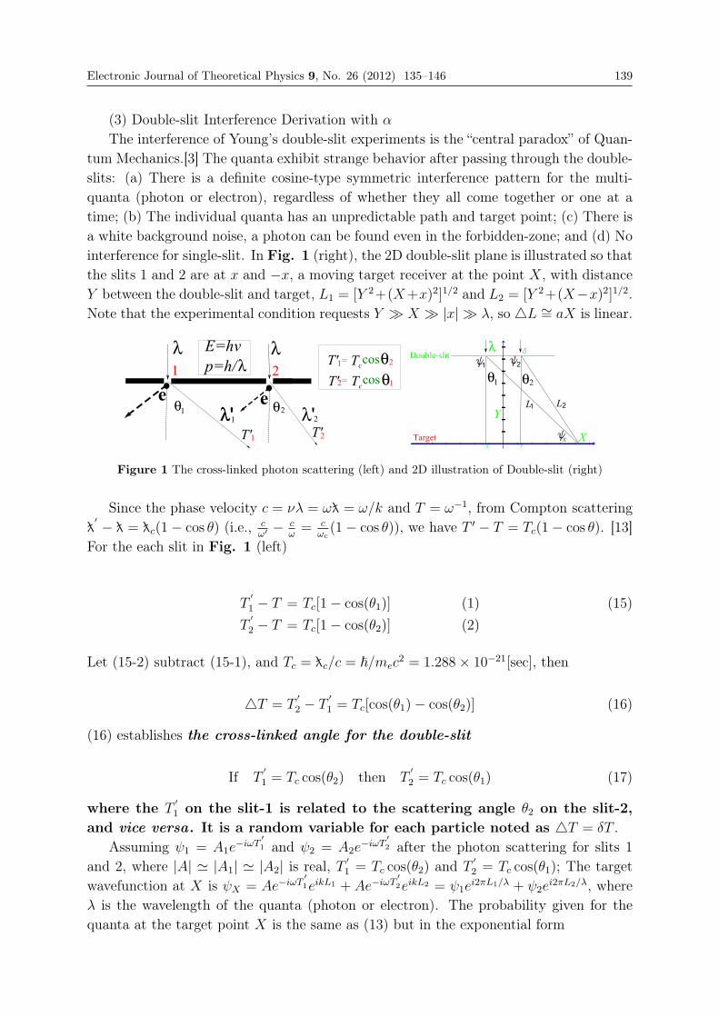
tum Mechanics.[3] The quanta exhibit strange behavior after passing through the double-slits: (a) There is a definite cosine-type symmetric interference pattern for the multi-quanta (photon or electron), regardless of whether they all come together or one at atime; (b) The individual quanta has an unpredictable path and target point; (c) There isa white background noise, a photon can be found even in the forbidden-zone; and (d) Nointerference for single-slit. In Fig. 1 (right), the 2D double-slit plane is illustrated so thatthe slits 1 and 2 are at x and −x, a moving target receiver at the point X, with distanceY between the double-slit and target, L1 = [Y 2+(X+x)2]1/2 and L2 = [Y 2+(X−x)2]1/2.Note that the experimental condition requests Y � X � |x| � λ, so �L ∼= aX is linear.

Figure 1 The cross-linked photon scattering (left) and 2D illustration of Double-slit (right)

Since the phase velocity c = νλ = ωň = ω/k and T = ω−1, from Compton scatteringň′ − ň = ňc(1− cos θ) (i.e., c

ω′ − cω= c

ωc(1− cos θ)), we have T ′ − T = Tc(1− cos θ). [13]

For the each slit in Fig. 1 (left)

T′1 − T = Tc[1− cos(θ1)] (1) (15)T′2 − T = Tc[1− cos(θ2)] (2)

Let (15-2) subtract (15-1), and Tc = ňc/c = �/mec2 = 1.288× 10−21[sec], then

�T = T′2 − T

′1 = Tc[cos(θ1)− cos(θ2)] (16)

(16) establishes the cross-linked angle for the double-slit

If T′1 = Tc cos(θ2) then T

′2 = Tc cos(θ1) (17)

where the T′1 on the slit-1 is related to the scattering angle θ2 on the slit-2,

and vice versa. It is a random variable for each particle noted as �T = δT .Assuming ψ1 = A1e

−iωT ′1 and ψ2 = A2e−iωT ′2 after the photon scattering for slits 1

and 2, where |A| |A1| |A2| is real, T ′1 = Tc cos(θ2) and T′2 = Tc cos(θ1); The target

wavefunction at X is ψX = Ae−iωT′1eikL1 + Ae−iωT

′2eikL2 = ψ1e

i2πL1/λ + ψ2ei2πL2/λ, where

λ is the wavelength of the quanta (photon or electron). The probability given for thequanta at the target point X is the same as (13) but in the exponential form


|ψX |2 = (Ae−iωT′1eikL1 + Ae−iωT

′2eikL2)(AeiωT

′1e−ikL1 + AeiωT

′2e−ikL2) (18)

= |A|2 · [1 + 1 + ei(kL1−ωT ′1−kL2+ωT′2) + e−i(kL1−ωT ′1−kL2+ωT

′2)]

= |A|2{ 2 + 2 cos[k(L1 − L2)− ω(T′1 − T

′2)]}

Whitenoise

Waveinterference

Particlescattering

= 2|A|2[1 + cos(k�L− ωδT′)]

space time

The angle term in (18) is same as 1�(p · r−Et) = (k · r−ωt) = k(r−ct) in (6), i.e., related

to the fine structure constant in (5). It is ňc = αa0 = α2

4πR∞ for the free electron and�

mic= mp

mi

αβa0 = mp

mi

α2

β1

4πR∞ for the atomic bonding electron in the Compton scattering.(18) clearly show that the wave-particle duality by the wave-vector k and the photon-frequency ω linked separately to the space �L and time δT ′ .

The visible photon-frequency ω ∼ 1014[Hz]. The term of ωδT ′ are random and smalleffect on the visible-light scattering by the tightly bound electron (mi � me). Therefore,the term 2π

λ(L1 − L2) = akX is the major-variable in control. The cosine term becomes

{−1, 0, 1} when 2πλ(L1−L2)−ω(T1−T2) = akX−ωδT ′ = {(2n±1)π, (n+ 1

2)π, 2nπ} where

k = 2πλ

, n = 0,±1,±2, · · · , and let |ψX |2 = {0, 2, 4)}|A|2. The continued distribution ischanges into a quantum interference pattern during coherence and cross-correlation.[14]Assuming A = sinc[k�L] and A1,2 = sinc[k(�L±x)], the graph of (18) matches perfectlywith experimental data from MIT for the far target using lasers (Fig. 2), 2 and Teachspinfor the near target with “one photon at a time” (Fig. 3).3 The scatter graph in Fig. 2and Fig. 3 clearly show that the interference pattern with the random scattering effectas the individual particle of “one photon at a time.”

Figure 2 The scatter graph of the probability density |ψX |2DS in (18) (top); and the Laserdouble-slit experimental data for the far target from MIT (bottom)

2 http://scripts.mit.edu/~tsg/www/demo.php?letnum=P%2010 (2011)3 http://www.teachspin.com/instruments/two_slit/experiments.shtml (2011)


Figure 3 The scatter graph of |ψX |2DS , |ψ1|2 and |ψ2|2 in (18) (left); and the “one photon at atime” double-slit experimental data for the near target from Teachspin (right)

(18) indicates that the double-slit experiment has the interference pattern (a) with arandom quantum scatting (b) and a background white noise (c). Notice that the cosinefunction is an even function responsible for making the symmetric interference patternappearing on the target plate. It also shows that there is no interference pattern forthe narrow single-slit (d), since |ψke

i2πLk/λ|2 = (Ake−iωtkeikLk)(Ake

iωtke−ikLk) = |Ak|2where k = 1, 2 (Fig. 3). As an exception, a slit which is wider than a wavelengthproduces Fraunhofer diffraction similar to the weak interference, due to the slit-edgeelectron-photon scattering effect. The probability for the diffraction of a wide single-slitat the target point X can be derived as a Taylor-Maclaurin series or Euler-Viete infiniteproduct,

|ψX |2SS = |A|2 = |sinc(akX)|2 = [∞∑

n=1(−1)n (akX)2n

(2n+1)!]2 (19)

= { ∞∏n=1

[1− (akXnπ

)2]}2 = [ ∞∏n=1

cos(akX2n

)]2

where akX = πdλsin θ and slit width d = 2x. Unlike θ in the Fraunhofer approximation

for the far field limitation, X can be measured directly regardless far or near target. (19)looks like but is not Gaussian distribution. Fig. 4 shows the graph of (19) comparedwith the single-slit diffraction experimental data using laser and adjustable slit-width.

Figure 4 The graph of the probability density |ψX |2SS in (19) (top); and the single-slit diffractionexperimental data from MIT (bottom)


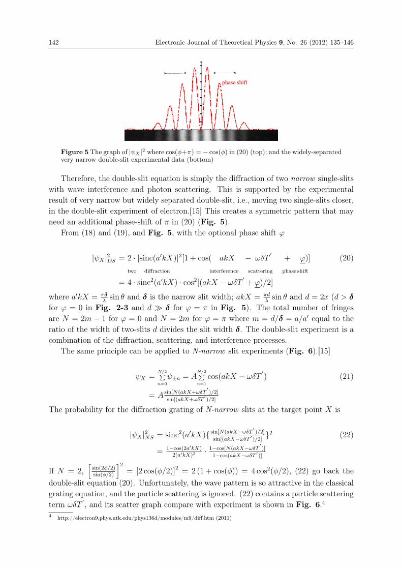
Figure 5 The graph of |ψX |2 where cos(φ+π) = − cos(φ) in (20) (top); and the widely-separatedvery narrow double-slit experimental data (bottom)

Therefore, the double-slit equation is simply the diffraction of two narrow single-slitswith wave interference and photon scattering. This is supported by the experimentalresult of very narrow but widely separated double-slit, i.e., moving two single-slits closer,in the double-slit experiment of electron.[15] This creates a symmetric pattern that mayneed an additional phase-shift of π in (20) (Fig. 5).

From (18) and (19), and Fig. 5, with the optional phase shift ϕ

|ψX |2DS = 2 · |sinc(a′kX)|2[1 + cos( akX − ωδT′

+ ϕ)] (20)two diffraction interference scattering phase shift

= 4 · sinc2(a′kX) · cos2[(akX − ωδT′+ ϕ)/2]

where a′kX = πδλsin θ and δ is the narrow slit width; akX = πd

λsin θ and d = 2x (d > δ

for ϕ = 0 in Fig. 2-3 and d � δ for ϕ = π in Fig. 5). The total number of fringesare N = 2m − 1 for ϕ = 0 and N = 2m for ϕ = π where m = d/δ = a/a′ equal to theratio of the width of two-slits d divides the slit width δ. The double-slit experiment is acombination of the diffraction, scattering, and interference processes.

The same principle can be applied to N-narrow slit experiments (Fig. 6).[15]

ψX =N/2∑n=0

ψ±n = AN/2∑n=1

cos(akX − ωδT′) (21)

= A sin[N(akX+ωδT′)/2]

sin[(akX+ωδT ′ )/2]

The probability for the diffraction grating of N-narrow slits at the target point X is

|ψX |2NS = sinc2(a′kX){ sin[N(akX−ωδT ′ )/2]sin[(akX−ωδT ′ )/2] }2 (22)

= 1−cos(2a′kX)2(a′kX)2

· 1−cos[N(akX−ωδT ′ )]1−cos(akX−ωδT ′ )]

If N = 2,[sin(2φ/2)sin(φ/2)

]2= [2 cos(φ/2)]2 = 2 (1 + cos(φ)) = 4 cos2(φ/2), (22) go back the

double-slit equation (20). Unfortunately, the wave pattern is so attractive in the classicalgrating equation, and the particle scattering is ignored. (22) contains a particle scatteringterm ωδT

′ , and its scatter graph compare with experiment is shown in Fig. 6.4

4 http://electron9.phys.utk.edu/phys136d/modules/m9/diff.htm (2011)


Figure 6 The scatter graph of the probability density |ψX |21,2,3,4,5,7 in (22) (top); and theN-narrow slits (1, 2, 3, 4, 5, 7) diffraction data (bottom)

In this model, the slit-edge electron-photon scattering plays a hidden role (each slit hastwo edges), which is linked to the fine structure constant.[7] Compton scattering creatingredshift has been confirmed by sunlight and the MIT double-slit experiment (Fig. 2).The fine structure constant must also play critical rule in the double-slit experiment ofelectron, neutron, He-atoms, and C-60 molecules. Fig. 7 shows that there is a classicaldistribution (or de-coherent) if the quanta-slit interaction is weak (e.g., the double-slitexperiment for neutron, C-60 and other heavy atoms). Other types of quantum scattering(e.g., Møller) may be involved. The Neutron double-slit data can be described as[16]

Figure 7 The scatter graph of the probability density |ψX |2NDS = |ψ1 + ψ2|2 + |ψ1|2 + |ψ2|2 in(23) (left); and the Neutron double-slit data (right)

Fig. 7 shows that many quanta have passed the slit without interaction (leaking), theyare not taking place in the interference. This is also true for the light-quanta passing awidely separated double-slit. The experiment for which-way also show the de-coherent bythe secondary scattering after the quanta passed slit.[17] It further prove that the quantumscattering is a critical issue behind the geometric parameters for the wave-pattern. Inother word, there will be no interference without quanta scattering. The finestructure constant is the magic hand behind the double-slit experiment. This modelclearly displays the particle-wave duality by particle scattering and wave-interference.


The quanta can be counted as one particle at a time, and the multi-quantas are displacedas the cosine-type wave-pattern in space. The electromagnetic wave frequency is in theregion of ω = kc = 100 ∼ 1024[Hz]. Since Tc = 1.288 × 10−21[sec], the double-slit waveinterference can be tested from soft-X-ray (1018[Hz]) to microwave (108[Hz]). The visiblelight (∼ 1014[Hz]) is a wave-like rather than the particle-like, and the γ-ray (1020−24[Hz])is a particle-like rather than the wave-like. This physical reality was obscured by thetrigonometric identities, however, there are many different versions of the classical gratingequations. From the discussion in section (2), the quantum physical principle is the sameand independent of the mathematical expression and coordinate system.

(4) Uncertainty Principle Derivation From α

In a thought experiment of the double-slit, Einstein suggested that the particle in-teract with the slit-well should consider the recoil of the wall and conservation of mo-mentum. The Compton scattering obeys the conservation of momentum. Bohr discussedthe double-slit and the uncertainty principle as v�p ≈ h/�t on the debate in 1927.[18]Landau rewrote the uncertainty principle as �P�t � �

cα1/2 in 1931. He also pointed out

a weakness in the interpretation of the uncertainty principle, such as, �E�t � �

2“does

not mean that the energy can not be measured with arbitrary accuracy within a shorttime.”[18] Here we show, the uncertainty principle can also be derived from thefine structure constant (2). From e2/c which has the same dimension with �, Et andp · r, for the spin-1/2 electron

�

2= 1

2e1e2αc

= 12e2

ve= 1

2e2

�x�t = 1

2�E�t = (23)

12

e2

�x2�t�x = 12mea�t�x = 1

2me�v�x = 1

2�Px�x

where E = e2/r, F = e2/r2 = ma, v = at and P = mv are the simple relationships inClassical physics. The orbital electron velocity is a variable vector that change directions.In (24), if �t deceases, �x will also decease and make �E increase; the sameis true for �x and �Px. This is the most simple and direct physical causality of theuncertainty principle. Experimentally, �x and the others can be defined as the standarddeviations, e.g.,

�x = σx = [ 1N

N∑i=1(xi − x)2]1/2 (24)

If �x → 0, then the symmetric standard deviation σPx � 12�Px. Therefore, for the

spin-1/2 particles

�E�t � �

2�Px�x � �

2(25)

Due to the conservation of angular momentum, the property of e1 must change if e2is altered. The electrons in an atom are high-speed (αc) charged particles. The distancebetween e1 and e2 is constantly adjusting, which causes the measurement uncertainty.The nucleon has a micro-motion and thus the electron orbit could not be a perfect cir-cle. The orthogonal and anti-commute pair [A, B] = ±i�, then �A�B ≥ �/2 given


by Heisenberg-Kennard.[19,20] There are many different mathematical versions of theuncertainty principle, again, the quantum reality is the same.

(5) Quantum Mechanics Postulates and αQuantum Mechanics is based on a number of postulates, such as

(1) The wavefunction Ψ determines everything that can be known about the system;(2) The operator Q acting on the wavefunction to determine the physical observable q;(3) The wave equation QΨn = qnΨn determines the eigenfunctions and eigenvalues;(4) The superposition of wavefunction Ψ =

∑anψn is an equivalent expression;

(5) The probability density is given by P = |Ψ|2 and the normalization is´V|Ψ|2dV = 1.

The interpretation of Quantum Mechanics has been of great debate among theoret-ical physicists, especially, Bohr and Einstein. Einstein was quoted: God does not playdice![21] However, he not only was a pioneer on Brownian motion, but also supported theBorn statistic explanation of Psi -function. He had argued for the realism, completeness,determinism, EPR-paradox, etc. What he was really looking for was A DEFINITERULE . In 1953, he said “That the Lord should play dice, all right; but that Heshould gamble according to definite rules, that is beyond me.”[22]

Here we show, the fine structure constant α is the cornerstone of quantum theory. Thewavefunction, Schrödinger equation and other quantum postulates, even the Uncertaintyprinciple can all be derived from it. Just as Pauli and Feynman pointed out: QuantumTheory is inconclusive without understanding the fine structure constant.[2,3]

Acknowledgment: The Author thanks Bernard Hsiao for discussion.

References

[1] M. Born, The Mysterious Number 137. Proc. Indian Acad. Sci. 2 (1935)

[2] W. Pauli, Exclusion Principle and Quantum Mechanics. Nobel Lecture (1946); TheConnection Between Spin and Statistics. Phys. Rev., 58, 716-722 (1940)

[3] R. P. Feynman, The Character of Physical Law, BBC Publications, (1965)

[4] A. Sommerfeld, Zur Quantentheorie der Spektrallinien. Ann. Phys. 51, 1-94 (1916); P.A. M. Dirac, The Principles of Quantum Mechanics (Fourth Edition). The ClarendonPress, Oxford, 272 (1958)

[5] E. Schrödinger, Quantisierung als Eigenwertproblem. Ann. Physik. (Leipzig) 79, 361,489 (1926); 80, 437 (1926); 81, 109 (1926)

[6] M. Born, Zur Quantenmechanik der Stoßvorgänge, Zeitschrift für Physik 37 863-867(1926); The Statistical Interpretations of Quantum Mechanics, Nobel Lecture (1954)

[7] K. Xiao, Dimensionless Constants and Blackbody Radiation Laws. EJTP, 8 379-388(2011)

[8] A. Einstein, Concerning an Heuristic Point of View Toward the Emission andTransformation of Light. Ann. Phys. 17 132-148 (1905)

[9] L. de Broglie, Ondes et Quanta. Compt. Ren. 177 507-510 (1923)

[10] M. Planck, Ueber das Gesetz der Energieverteilung im Normalspectrum. Ann. Phys.309 553–563 (1901)


[11] P. A. M. Dirac, Zur Quantentheorie des Elektrons, Leipziger Vorträge(Quantentheorie und Chemie), 85-94 (1928)

[12] J. W. Gibbs, Elementary Principles in Statistical Mechanics. New York: Scribner(1902)

[13] A. Compton, A Quantum Theory of the Scattering of X-Rays by Light Elements.Phys. Rev. 21, 483-502 (1923)

[14] R. J. Glauber, The quantum theory of optical coherence. Phys. Rev., 130, 2529-2539(1963)

[15] C Jönsson, Interferenz von Elektronen am Doppelspalt. Zeitschrift für Physik, 161,454-474 (1961); Electron Diffraction at Multiple Slit. Am. J. Phys. 42, 4-11 (1974)

[16] A. Zeilinger, et. al., Single- and double-slit diffraction of neutron. Rev. Mod. Phys.,60, 1067-1073 (1988); D. S. Weiss, et. al., Precision Measurement of the Photon Recoilof an Atom Using Atomic Interferometry. Phys. Rev. Lett. 70, 2706-2709 (1993)

[17] M. S. Chapman, et. al., Photon Scattering from Atoms in an Atom Interferometer:Coherence Lost and Regained, Phys. Rev. Lett. 75 3783-3787 (1995)

[18] N. Bohr, Discuss With Einstein on Epistemological Problems in Atomic Physics,(1949); L. D. Landau, R. Peierls, Extension of The Uncertainty Principle toRelativistic Quantum Theory. (1931) in Quantum Theory and Measurement. Ed.J. A. Wheeler and W. H. Zurek, 9-49, 465-476 (1983)

[19] W. Heisenberg, Über den anschaulichen Inhalt der quantentheoretischen Kinematikund Mechanik, Zeitschrift für Physik 43, 172-198 (1927)

[20] E. H. Kennard, Zur Quantenmechanik einfacher Bewegungstypen. Zeitschrift fürPhysik 44, 326-352 (1927)

[21] A. Einstein, Letter to Max Born (4 December 1926); The Born-Einstein Letters(translated by Irene Born) Walker and Company, New York, (1971)

[22] A. Einstein, quoted in J. Wheeler, W. Zurek, Quantum and Measurement, PrincetonU. Oress, p8 (1983)

the fine structure constant and interpretations of … · ejtp 9, no. 26 (2012) 135–146...

Documents