the florida state university massively … · the florida state university college of arts and...

THE FLORIDA STATE UNIVERSITY

COLLEGE OF ARTS AND SCIENCES

MASSIVELY PARALLEL ALGORITHMS FOR CFD SIMULATION AND

OPTIMIZATION ON HETEROGENEOUS MANY-CORE ARCHITECTURES

By

AUSTEN C. DUFFY

A Dissertation submitted to theDepartment of Mathematicsin partial fulfillment of the

requirements for the degree ofDoctor of Philosophy

Degree Awarded:Spring Semester, 2011

The members of the committee approve the dissertation of Austen C. Duffy defended on

March 15, 2011.

Mark SussmanProfessor Directing Dissertation

M. Yousuff HussainiProfessor Co-Directing Dissertation

Robert Van EngelenUniversity Representative

Nick CoganCommittee Member

Kyle GallivanCommittee Member

Approved:

Philip Bowers, Chair, Department of Mathematics

Joseph Travis, Dean, College of Arts and Sciences

The Graduate School has verified and approved the above-named committee members.

ii

This dissertation is dedicated to the memory of my father, Francis J. Duffy, who passedaway in September of 2010. Having never graduated from high school himself, and havingworked in the bleak Pennsylvania steel industry throughout my early life, he always pushedfor and encouraged my continuing education so that I might have a better life than his.

iii

ACKNOWLEDGMENTS

I would first like to thank my advisor Mark Sussman and my co-advisor Yousuff Hussainifrom whom I have learned much over the last several years. I would like to thank my othercommittee members for their help in completing this dissertation and for the valuable in-sight each has provided in the various topics that have comprised my graduate research.I would like to thank the Florida State University Mathematics Department for support-ing me as a teaching assistant in my first few years as a graduate student. I would like toacknowledge the sources of my research assistantship funding, the National Science Founda-tion under grants DMS-1016381 and DMS-0713256 and the Office of Naval Research undergrant N00014-04-1-0709, and I thank both organizations for their vital contributions to thetraining and education of America’s young scientists, engineers and mathematicians likemyself. I would like to thank the National Institute of Aerospace and NASA Langley Re-search Center for supporting me as a visiting researcher, and in particular Dana Hammondand Eric Nielsen of the Computational AeroSciences Branch. Finally, I would like to thankmy family, my friends and my soon to be wife Melissa for just always being there for methrough these difficult years.

iv

TABLE OF CONTENTS

List of Tables . . . . . . . . . . . . . . . . . . . . . . . . . . . . . . . . . . . . . . . . vii

List of Figures . . . . . . . . . . . . . . . . . . . . . . . . . . . . . . . . . . . . . . . xi

Abstract . . . . . . . . . . . . . . . . . . . . . . . . . . . . . . . . . . . . . . . . . . . xvi

1 Introduction 1

1.1 Motivation: Gradient Free Optimization . . . . . . . . . . . . . . . . . . . . 1

1.2 Motivation: Towards Computation at the Exascale . . . . . . . . . . . . . . 2

1.3 The Bigger Picture: Advancing Simulation Based Design in CFD . . . . . . 3

1.4 Background and Literature Review . . . . . . . . . . . . . . . . . . . . . . . 3

1.4.1 Numerical Optimization and Simulation Based Design . . . . . . . . 4

1.4.2 Accelerating CFD Codes on Hybrid Many-Core Architectures . . . . 6

2 PDE Constrained Optimization 8

2.1 Adjoint Methods . . . . . . . . . . . . . . . . . . . . . . . . . . . . . . . . . 8

2.1.1 Continuous Adjoint Method . . . . . . . . . . . . . . . . . . . . . . . 9

2.1.2 Discrete Adjoint Method . . . . . . . . . . . . . . . . . . . . . . . . 9

2.1.3 Linear Example Problem . . . . . . . . . . . . . . . . . . . . . . . . 11

2.1.4 Nonlinear Example Problem . . . . . . . . . . . . . . . . . . . . . . . 14

2.1.5 A Matrix Free Representation of the Discrete Adjoint Problem . . . 15

2.2 Parallel Derivative Free Methods . . . . . . . . . . . . . . . . . . . . . . . . 18

2.2.1 The Multidirectional Search Method . . . . . . . . . . . . . . . . . . 19

2.2.2 A Multigriding Strategy for the Multidirectional Search Method . . 21

2.3 Numerical Results and Discussion . . . . . . . . . . . . . . . . . . . . . . . . 21

2.3.1 Linear Advection Problem . . . . . . . . . . . . . . . . . . . . . . . . 24

2.3.2 Nonlinear Burgers Equation Problem . . . . . . . . . . . . . . . . . . 24

2.3.3 Multigrid-Multidirectional Search Strategies . . . . . . . . . . . . . . 29

2.3.4 Discussion of Numerical Results . . . . . . . . . . . . . . . . . . . . 39

3 CFD Code Acceleration 42

3.1 Graphics Processors and Hybrid Computing Architectures . . . . . . . . . . 42

3.2 The Coupled Level-Set and Volume-of-Fluid Method . . . . . . . . . . . . . 43

3.2.1 Solution of the Pressure Poisson Equation . . . . . . . . . . . . . . . 44

3.2.2 GPU Acceleration of the Pressure Projection Step on a Uniform Grid 46

3.2.3 An Improved Projection Algorithm for Adaptive Meshes . . . . . . . 48

3.2.4 2D Bubble . . . . . . . . . . . . . . . . . . . . . . . . . . . . . . . . 55

v

3.2.5 3D Bubble . . . . . . . . . . . . . . . . . . . . . . . . . . . . . . . . 553.2.6 3D Whale . . . . . . . . . . . . . . . . . . . . . . . . . . . . . . . . . 58

3.3 FUN3D . . . . . . . . . . . . . . . . . . . . . . . . . . . . . . . . . . . . . . 583.3.1 Mathematical Formulation . . . . . . . . . . . . . . . . . . . . . . . 623.3.2 Parallelization and Scaling . . . . . . . . . . . . . . . . . . . . . . . . 623.3.3 GPU Acceleration . . . . . . . . . . . . . . . . . . . . . . . . . . . . 633.3.4 GPU Distributed Sharing Model . . . . . . . . . . . . . . . . . . . . 653.3.5 CUDA Subroutines . . . . . . . . . . . . . . . . . . . . . . . . . . . . 65

3.4 Test Problems . . . . . . . . . . . . . . . . . . . . . . . . . . . . . . . . . . . 673.4.1 Test Problem 1 . . . . . . . . . . . . . . . . . . . . . . . . . . . . . . 673.4.2 Test Problem 2 . . . . . . . . . . . . . . . . . . . . . . . . . . . . . . 67

3.5 FUN3D Results and Discussion . . . . . . . . . . . . . . . . . . . . . . . . . 673.5.1 Single Core Performance . . . . . . . . . . . . . . . . . . . . . . . . . 693.5.2 Multiple Core Performance . . . . . . . . . . . . . . . . . . . . . . . 713.5.3 Discussion . . . . . . . . . . . . . . . . . . . . . . . . . . . . . . . . . 71

4 Future Research 75

4.1 Towards the Computational Design of Microfluidic Structures . . . . . . . . 75

5 Conclusion 78

A FUN3D Timing Data 80

Bibliography . . . . . . . . . . . . . . . . . . . . . . . . . . . . . . . . . . . . . . . . 85

Biographical Sketch . . . . . . . . . . . . . . . . . . . . . . . . . . . . . . . . . . . . 91

vi

LIST OF TABLES

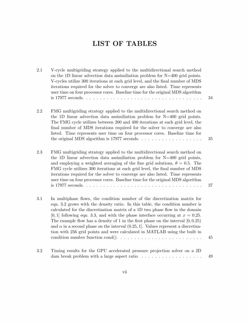
2.1 V-cycle multigriding strategy applied to the multidirectional search methodon the 1D linear advection data assimiliation problem for N=400 grid points.V-cycles utilize 300 iterations at each grid level, and the final number of MDSiterations required for the solver to converge are also listed. Time representsuser time on four processor cores. Baseline time for the original MDS algorithmis 17977 seconds. . . . . . . . . . . . . . . . . . . . . . . . . . . . . . . . . . . 34

2.2 FMG multigriding strategy applied to the multidirectional search method onthe 1D linear advection data assimiliation problem for N=400 grid points.The FMG cycle utilizes between 200 and 400 iterations at each grid level, thefinal number of MDS iterations required for the solver to converge are alsolisted. Time represents user time on four processor cores. Baseline time forthe original MDS algorithm is 17977 seconds. . . . . . . . . . . . . . . . . . . 35

2.3 FMG multigriding strategy applied to the multidirectional search method onthe 1D linear advection data assimiliation problem for N=400 grid points,and employing a weighted averaging of the fine grid solutions, θ = 0.5. TheFMG cycle utilizes 300 iterations at each grid level, the final number of MDSiterations required for the solver to converge are also listed. Time representsuser time on four processor cores. Baseline time for the original MDS algorithmis 17977 seconds. . . . . . . . . . . . . . . . . . . . . . . . . . . . . . . . . . . 37

3.1 In multiphase flows, the condition number of the discretization matrix foreqn. 3.2 grows with the density ratio. In this table, the condition number iscalculated for the discretization matrix of a 1D two phase flow in the domain[0, 1] following eqn. 3.3, and with the phase interface occurring at x = 0.25.The example flow has a density of 1 in the first phase on the interval [0, 0.25)and α in a second phase on the interval (0.25, 1]. Values represent a discretiza-tion with 256 grid points and were calculated in MATLAB using the built incondition number function cond(). . . . . . . . . . . . . . . . . . . . . . . . . 45

3.2 Timing results for the GPU accelerated pressure projection solver on a 2Ddam break problem with a large aspect ratio . . . . . . . . . . . . . . . . . . 49

vii

3.3 Timing results for a single pressure solve for the new MGPCG AMR algorithmalong with the old MG AMR algorithm and the PCG algorithm for the 3Daxisymmetric test bubble. The new MGPCG algorithm is faster than the oldMG AMR algorithm in nearly every scenario. Grid sizes for a fixed blockingfactor and number of adaptive levels are identical for each method. . . . . . . 57

3.4 Speedup factor for the new MGPCG AMR method over the original MG AMRmethod on the 3D axisymmetric test bubble problem. The new algorithmoutperforms the old by an increasing margin as both the blocking factor andthe number of adaptive levels are increased. It can be seen that the benefitsof the new method are not realized in the case of large blocking factors and asingle adaptive level. . . . . . . . . . . . . . . . . . . . . . . . . . . . . . . . . 57

3.5 Timing results for a single pressure solve for the new MGPCG AMR algorithmalong with the old MG AMR algorithm and the PCG algorithm for a 3D testbubble. . . . . . . . . . . . . . . . . . . . . . . . . . . . . . . . . . . . . . . . 59

3.6 Speedup factor for the new MGPCG AMR method over the original MG AMRmethod on the 3D test problem of simulating a gas bubble rising through aliquid phase. . . . . . . . . . . . . . . . . . . . . . . . . . . . . . . . . . . . . 59

3.7 Timing results for a single pressure solve for the new MGPCG AMR algorithmalong with the old MG AMR algorithm and the PCG algorithm for flow pasta 3D whale. . . . . . . . . . . . . . . . . . . . . . . . . . . . . . . . . . . . . . 61

3.8 Speedup factor for the new MGPCG AMR method over the original MG AMRmethod on the 3D test problem of flow past a 3D whale. . . . . . . . . . . . . 61

3.9 FUN3D Grid partitioning over 8 processor cores, showing that node distribu-tions are fairly well balanced. . . . . . . . . . . . . . . . . . . . . . . . . . . . 67

3.10 Single core performance results for routine gs gpu on test problem 1 using theGTX 480 WS. . . . . . . . . . . . . . . . . . . . . . . . . . . . . . . . . . . . 69

3.11 Single core performance results for routine gs gpu on test problem 1 using theGTX 470 BC. . . . . . . . . . . . . . . . . . . . . . . . . . . . . . . . . . . . . 70

3.12 Timing results for routine gs mpi2 on test problem 1 using the GTX 480 WS. 71

3.13 Timing results for routine gsmpi2 on test problem 1 using 1 node of the GTX470 BC. . . . . . . . . . . . . . . . . . . . . . . . . . . . . . . . . . . . . . . . 71

3.14 Timing results for routine gsmpi2 on test problem 1 using 2 nodes of the GTX470 BC. . . . . . . . . . . . . . . . . . . . . . . . . . . . . . . . . . . . . . . . 72

viii

3.15 GPU architecture evolution from G80, which approximately coincided with therelease of Intel’s quad core CPUs, to Fermi which coincided with the releaseof Intel’s six core processors. GPU advancements over the last few years havenoticeably outpaced those of CPUs. Representative GPUs are: G80-GeForce8800 GT, GT200-Tesla C1060, Fermi-Tesla C2050. 1shared memory, 2 texturememory, 3Configurable L1/shared memory. . . . . . . . . . . . . . . . . . . . 74

A.1 Test problems used in this study. * approximate. . . . . . . . . . . . . . . . . 81

A.2 Timing results for routine gs gpu on test problem 1 using the TESLA RC. . 81

A.3 Timing results for routine gs mpi0 on test problem 1 using the GTX 480 WS. 81

A.4 Timing results for routine gs mpi0 on test problem 1 using 1 node of the GTX470 BC. . . . . . . . . . . . . . . . . . . . . . . . . . . . . . . . . . . . . . . . 81

A.5 Timing results for routine gs mpi0 on test problem 1 using 2 nodes of the GTX470 BC. . . . . . . . . . . . . . . . . . . . . . . . . . . . . . . . . . . . . . . . 81


A.7 Timing results for routine gs mpi1 on test problem 1 using 1 node of the GTX470 BC. . . . . . . . . . . . . . . . . . . . . . . . . . . . . . . . . . . . . . . . 82

A.8 Timing results for routine gs mpi1 on test problem 1 using 2 nodes of the GTX470 BC. . . . . . . . . . . . . . . . . . . . . . . . . . . . . . . . . . . . . . . . 82

A.9 Timing results for routine gs mpi2 on test problem 1 using 1 node of theTESLA RC. . . . . . . . . . . . . . . . . . . . . . . . . . . . . . . . . . . . . 82

A.10 Timing results for routine gs gpu on test problem 2 using the GTX 480 WS. 82

A.11 Timing results for routine gs gpu on test problem 2 using the GTX 470 BC. 83


A.13 Timing results for routine gs mpi2 on test problem 2 using two nodes of theGTX 470 BC machine. . . . . . . . . . . . . . . . . . . . . . . . . . . . . . . 83


A.15 Timing results for routine gs mpi2 on test problem 3 using the GTX 480 WSmachine. . . . . . . . . . . . . . . . . . . . . . . . . . . . . . . . . . . . . . . 83

A.16 Timing results for routine gs mpi2 on test problem 3 using two nodes of theGTX 470 BC machine. GPU Memory is insufficient for sharing among 4threads, the problem must be split across two GPUs. . . . . . . . . . . . . . 83

ix


A.18 Timing results for routine gs mpi2 on test problem 4 using eight nodes of theTESLA RC machine. . . . . . . . . . . . . . . . . . . . . . . . . . . . . . . . 84

x

LIST OF FIGURES

2.1 2-Simplex (Left): A two dimensional triangle made by connecting 3 vertices. 3-Simplex (Right): A 3 dimensional tetrahedron made of triangles by connecting4 vertices . . . . . . . . . . . . . . . . . . . . . . . . . . . . . . . . . . . . . . 19

2.2 Multigrid cycling schemes tested in this work include the V-Cycle and the fullmultigrid cycle (FMG). . . . . . . . . . . . . . . . . . . . . . . . . . . . . . . 22

2.3 Adjoint solution for linear advection problem. Left: Recovered IC for 64 gridpoints (U) versus exact IC (data). Right: Comparison of the advected solu-tions. β = 1.0, ∆x = 1

32 , ∆t = 0.01. Requires 200 iterations for convergenceand runs in 1.945 seconds on a single CPU core. . . . . . . . . . . . . . . . . 25

2.4 MDS solution for linear advection problem. Left: Recovered IC for 64 gridpoints (U) versus exact IC (data). Right: Comparison of the advected solu-tions. β = 1.0, ∆x = 1

32 , ∆t = 0.01. Requires 8470 iterations for convergenceand runs in 50.183 seconds on four CPU cores. . . . . . . . . . . . . . . . . . 25




64 , ∆t = 0.01. Requires 25330 iterations for convergenceand runs in 553.261 seconds on four CPU cores. . . . . . . . . . . . . . . . . 26

2.7 Adjoint solution for linear advection problem. Left: Recovered IC for 256grid points (U) versus exact IC (data). Right: Comparison of the advectedsolutions. β = 1.0, ∆x = 1

128 , ∆t = 0.01. Requires 5700 iterations forconvergence and runs in 476.535 seconds on a single CPU core. . . . . . . . . 27


128 , ∆t = 0.01. Requires 28060 iterations for conver-gence and runs in 2394.518 seconds on four CPU cores. . . . . . . . . . . . . 27

xi




200 , ∆t = 0.01. Requires 20690 iterations for conver-gence and runs in 4694.7679 seconds on four CPU cores. . . . . . . . . . . . . 28

2.11 Adjoint solution for non-linear Burger’s equation problem. Left: Recovered IC(U) versus exact IC (data), t=0.05. Right: Comparison of the final solutions.β = 1.0, ∆x = 1

48 , ∆t = 0.005, µ = 0.001. Requires 200 iterations forconvergence and runs in 4.339 seconds on a single CPU core. . . . . . . . . . 29

2.12 MDS solution for non-linear Burger’s equation problem. Left: Recovered IC(U) versus exact IC (data), t=0.05. Right: Comparison of the final solutions.β = 1.0, ∆x = 1

48 , ∆t = 0.005, µ = 0.001. Requires 720 iterations forconvergence and runs in 2.763 seconds on four CPU cores. . . . . . . . . . . . 30


48 , ∆t = 0.005, µ = 0.001. Requires 200 iterations forconvergence and runs in 27.599 seconds on a single CPU core. . . . . . . . . 30


48 , ∆t = 0.005, µ = 0.001. Requires 1470 iterations forconvergence and runs in 10.354 seconds on four CPU cores. . . . . . . . . . . 31




48 , ∆t = 0.005, µ = 0.001. Requires 3220 iterations forconvergence and runs in 30.021 seconds on four CPU cores. . . . . . . . . . . 32



xii


48 , ∆t = 0.005, µ = 0.001. Requires 10690 iterations forconvergence and runs in 120.272 seconds on four CPU cores. . . . . . . . . . 33




48 , ∆t = 0.005, µ = 0.001. Requires 45620 iterations forconvergence and runs in 704.615 seconds on four CPU cores. . . . . . . . . . 34

2.21 MGMDS solution for linear advection problem using an FMG cycle with 200iterations at each level. Left: Recovered IC for 400 grid points (U) versus exactIC (data). Right: Comparison of the advected solutions. β = 1.0, ∆x = 1

200 ,∆t = 0.01. . . . . . . . . . . . . . . . . . . . . . . . . . . . . . . . . . . . . . 35

2.22 MGMDS solution for linear advection problem using an FMG cycle with 300iterations at each level. Left: Recovered IC for 400 grid points (U) versus exactIC (data). Right: Comparison of the advected solutions. β = 1.0, ∆x = 1

200 ,∆t = 0.01. . . . . . . . . . . . . . . . . . . . . . . . . . . . . . . . . . . . . . 36

2.23 MGMDS solution for linear advection problem using 2 V-cycles with 300 iter-ations at each level. Left: Recovered IC for 400 grid points (U) versus exactIC (data). Right: Comparison of the advected solutions. β = 1.0, ∆x = 1

200 ,∆t = 0.01. Requires 2 V-cycles plus 10350 final MDS iterations for conver-gence and runs in 2515.487 seconds on four CPU cores. . . . . . . . . . . . . 36

2.24 MGMDS solution for nonlinear Burger’s problem using an FMG cycle. Left:Recovered IC for 256 grid points (U) versus exact IC (data). Right: Compar-ison of the advected solutions. β = 1.0, ∆x = 1

48 , ∆t = 0.005, µ = 0.001. . . . 37

2.25 MGMDS IC recovery for a 1D linear advection data assimilation problem usingan FMG cycle employing a weighted averaging of the fine grid solution. Usingmore than one FMG cycle results in a smoothing effect on the solution data.Top Left: 1 FMG cycle. Top Right: 2 FMG cycles. Bottom Left: 3 FMGcycles. Bottom Right: 4 FMG cycles. β = 1.0, ∆x = 1

200 , ∆t = 0.01 for allfigures. . . . . . . . . . . . . . . . . . . . . . . . . . . . . . . . . . . . . . . . 38

2.26 Adjoint nonlinear IC Recovery, 5 observations. Left: Recovered IC (U) versusexact IC (data), t=0.5. Right: Comparison of the final solutions. β = 1.0,∆x = 1

48 , ∆t = 0.005, µ = 0.001. . . . . . . . . . . . . . . . . . . . . . . . . . 39

xiii


48 , ∆t = 0.005, µ = 0.001. . . . . . . . . . . . . . . . . . . . . . . . . . 40


48 , ∆t = 0.005, µ = 0.001. . . . . . . . . . . . . . . . . . . . . . . . . . 40

3.1 Example 1D discretization for the pressure Poisson equation . . . . . . . . . 45

3.2 The condition number of the discretization matrix is not as sensitive to theproblem geometry as it is to the density ratio. The corresponding conditionnumbers for these figures are 6,132,300 (left), 1,861,000 (middle) and 2,548,900(right) using a 2D version of discretization eqn. 3.3 on a 64 x 64 grid. . . . . 45

3.3 Adaptive mesh hierarchy in 2D. To compute the solution at level l+1, the MGAMR algorithm (alg. 9) requires calculations at levels l and l-1. . . . . . . . 52

3.4 An MGPCG smoother can only achieve a single coarsening step on the illus-trated fine level; then one must use PCG as a bottom solver on the “irregularlyshaped” coarsest domain. On the other hand, our new MG preconditionercoarsens only one level too, but the bottom solver is MGPCG on the wholenon-“irregularly shaped” domain. The bottom solver of our new method cancoarsen two more times. . . . . . . . . . . . . . . . . . . . . . . . . . . . . . . 53

3.5 Coarse and fine grid levels depicting real and fictitious cells. . . . . . . . . . . 55

3.6 AMR grids for a rising 3D axisymmetric bubble. The representative grids alluse a blocking factor of two and contain a) one adaptive level, b) two adaptivelevels, c) three adaptive levels, and d) four adaptive levels. . . . . . . . . . . 56

3.7 Mesh for a 3D rising bubble with 2 adaptive levels and a blocking factor of 4. 58

3.8 Mesh for a 3D whale with 2 adaptive levels. . . . . . . . . . . . . . . . . . . . 60

3.9 Parallel scaling results for FUN3D. Problems are given by node size, withM equating to millions of nodes. There are approximately 6 times as manytetrahedral cells as there are nodes for a given problem size. Ares is a rocketgeometry and DPW grids represent aircraft configurations from AIAA DragPrediction Workshops. The linear dashed line represents ideal scaling. . . . . 63

3.10 Test problem 1 grid (left) and GPU computed pressure solution for pp∞

(right).Generic wing-body geometry, contains 339,206 nodes and 1,995,247 tetrahedralcells. Pressure solution obtained at convergence of the FUN3D solver (132iterations). Inviscid, Mach Number = 0.3, Angle of Attack = 2.0 degrees. . . 68

xiv

3.11 Test problem 2 grid (left) and GPU computed pressure solution for pp∞

(right).DLR-F6 wing-body configuration, contains approximately 650,000 nodes and3.9 million tetrahedral cells. Turbulent, Mach Number = 0.76, Angle of Attack= 0.0 degrees, Reynolds Number = 1, 000, 000. . . . . . . . . . . . . . . . . . 68

3.12 CPU and GPU performances for a single PS5 sweep with varying test casesizes. Tests were run on a single core of an Intel Xeon 5080 CPU mated witha single NVIDIA GTX 480 GPU. . . . . . . . . . . . . . . . . . . . . . . . . . 70

3.13 Strong scaling within a single node for a single sweep of the PS5 subroutineusing CUDA version gs mpi2. Tests were run on 2 nodes of a Beowulf GPUcluster, each running an AMD Athlon II X4 quad core processor and NvidiaGTX 470 GPU. Strong scaling results use a 340,000 grid point test problemon one node. . . . . . . . . . . . . . . . . . . . . . . . . . . . . . . . . . . . . 72

3.14 Weak scaling across two compute nodes for a single sweep of the PS5 subrou-tine using CUDA version gs mpi2. Tests were run on 2 nodes of a BeowulfGPU cluster, each running an AMD Athlon II X4 quad core processor andNvidia GTX 470 GPU. Weak scaling results use a 340,000 grid point testproblem on one node, and a 650,000 grid point problem distributed across 2nodes. Weak scaling times are per 100,000 grid points. . . . . . . . . . . . . . 73

4.1 Microfluidic T-junction experiment from Roper’s laboratory (FSU Chemistry)showing a T-junction geometry with a droplet traveling via a carrier fluid. . . 77

4.2 Numerical simulations of two fluids in a microfluidic T-junction using theCLSVOF code and experimental setups from Roper’s Lab. . . . . . . . . . . 77

xv

ABSTRACT

In this dissertation we provide new numerical algorithms for use in conjunction with simula-tion based design codes. These algorithms are designed and best suited to run on emergingheterogenous computing architectures which contain a combination of traditional multi-core processors and new programmable many-core graphics processing units (GPUs). Wehave developed the following numerical algorithms (i) a new Multidirectional Search (MDS)method for PDE constrained optimization that utilizes a Multigrid (MG) strategy to accel-erate convergence, this algorithm is well suited for use on GPU clusters due to its parallelnature and is more scalable than adjoint methods (ii) a new GPU accelerated point im-plicit solver for the NASA FUN3D code (unstructured Navier-Stokes) that is written in theCompute Unified Device Architecture (CUDA) language, and which employs a novel GPUsharing model, (iii) novel GPU accelerated smoothers (developed using PGI Fortran withaccelerator compiler directives) used to accelerate the multigrid preconditioned conjugategradient method (MGPCG) on a single rectangular grid, and (iv) an improved pressureprojection solver for adaptive meshes that is based on the MGPCG method which requiresfewer grid point calculations and has potential for better scalability on hetergeneous clus-ters. It is shown that a multigrid - multidirectional search (MGMDS) method can run upto 5.5X faster than the MDS method when used on a one dimensional data assimilationproblem. It is also shown that the new GPU accelerated point implicit solver of FUN3D isup to 5.5X times faster than the CPU version and that the solver can perform up to 40%faster on a single GPU being shared by four CPU cores. It is found that GPU acceleratedsmoothers for the MGPCG method on uniform grids can run over 2X faster than the non-accelerated versions for 2D problems, and that the new MGPCG pressure projection solverfor adaptive grids is up to 4X faster than the previous MG algorithm.

xvi

CHAPTER 1

INTRODUCTION

Traditional high performance computers containing advanced multi-core processors are in-creasingly being mated with add on specialty hardware such as cell processors, field pro-grammable gate arrays (FPGAs), and graphics processing units (GPUs), creating newbreeds of heterogenous computer architectures [23]. The emergence of these heterogeneousmany-core computing platforms has allowed for the creation of a new wave of software thatexploits an additional level of fine grain parallelism not available to traditional high perfor-mance computers. When properly programmed, these systems have given way to drasticreductions in computation time for problems across the spectrum of science and engineer-ing. In this work we develop algorithms designed to exploit the unprecedented levels ofmass parallelism [23] these hybrid architectures can provide on the path towards exascalecomputing. The primary mathematical focus of this dissertation is the development ofnovel simulation based design (SBD) algorithms that are scalable on heterogeneous plat-forms. The following items have been developed: (i) a gradient free ‘black box’ optimizer forPDE constrained optimization that is trivially parallelizable and more scalable than adjointmethods which converge more rapidly. (ii) CFD solvers that exploit GPUs and MPI. (iii) anew MGPCG algorithm for block structured adaptive grids that requires fewer grid pointcalculations than the previous method and is intuitively more scalable on heterogeneouscomputer architectures. In addition to heterogenous scalability, another underlying themefound in this work is the use of multigriding strategies which are used to accelerate both agradient free optimizer and the pressure projection solver of an incompressible multiphaseflow solver. Multigrid methods together with block structured data storage enable moreefficient use of cache making them well suited for heterogeneous computers. Since this workcombines research from distinct areas, we will provide some motivation from each.

1.1 Motivation: Gradient Free Optimization

Numerical optimization is a broad field that can essentially be broken down into twobasic categories, derivative and derivative free. Derivative based methods draw directlyfrom calculus where the minimum (or maximum) of a function can be found simply byfinding the point where the derivative or gradient is zero. Numerical optimization methodsthat are founded in locating this point by using approximations to the derivative can beconsidered rather efficient even in the slowest converging case (steepest descent) when given

1

the alternative. It is, however, sometimes the case that gradient information is not avail-able, and less efficient alternative methods for numerically finding optimal points becomesnecessary. Gradient free methods draw upon various inspirations for locating an optima,from simply checking many random points (Monte Carlo methods) to the physical processof cooling (simulated annealing) to the biological process of evolution (genetic algorithms).Gradient free methods have many redeeming qualities, most notably that they tend to behighly robust and are trivially parallelizable in many cases. Unfortunately, gradient freemethods all seem to fall well short of their derivative based counterparts when consideringthe convergence rate, and so we would consider methods which can significantly reduce thesolution time for these methods highly desirable.

1.2 Motivation: Towards Computation at the Exascale

High performance computing systems are undergoing a rapid shift towards the couplingof add-on hardware, such as graphics processing units (GPUs), Cell processors and field pro-grammable gate arrays (FPGAs), with traditional multicore CPU’s. Hybrid clusters possessunprecedented price to performance ratios and high energy efficiency, having placed in thetop supercomputer rankings [1], and dominated the Green500 list [2]. We note that theChinese Tianhe-1A, a supercomputer employing Nvidia Fermi architecture GPUs, recentlysurpassed the Cray based ‘Jaguar’ of Oak Ridge National Laboratory as the worlds fastestcomputer [1]. GPU clusters are also being used for research in large scale hybrid computingin the U.S., including the Lincoln Tesla cluster at the National Center for SupercomputingApplications [49]. Plans to build many more of these machines in the very near future arealready underway, and while new codes can be developed with this in mind, an emergingchallenge in this modern heterogeneous computing landscape is updating old software tomake best use of newly available hardware.

An exascale roadmap [23] has been developed by leading computing researchers fromacademia and industry to address the issues involved with the transition from petascale toexascale computing. While this report discusses numerous issues including the computinginfrastrcture, power awareness and fail safe algorithms for many component systems, someimportant highlights we would like to emphasize from [23] include

• Exascale systems are expected to have a huge number of nodes, with many-core par-allelism existing within each node via accelerators such as GPUs, yielding a heteroge-neous computing environment.

• Memory heirarchies will be complex, programming models will need to exploit datalocality.

• There is a large body of existing scalable applications that need to be migrated towardsexascale.

• Exascale computing provides new opportunities for multi-scale, multi-physics andmulti-disciplinary applications.

2

• Algorithms will need to be architecturally aware - adapting to possible heterogeneousenvironments that they find themselves in.

While it is in general true that a code will see maximum benefit if it is designed fromthe ground up with available GPUs in mind, there are many widely used legacy codeswhose development has spanned multiple decades, and for which this is not an option. Inthese scenarios, the use of accelerator models in which tasks with large amounts of dataparallelism are ported to GPU code may provide the best solution. While some GPU codescan demonstrate multiple orders of magnitude speedup, additional constraints will likelyprevent existing high level computational fluid dynamics (CFD) codes from realizing thesegains, particularly when they have already been highly optimized for large scale parallelcomputation, or when the underlying spatial discretization is unstructured. Additionally,architectures with many CPU cores typically need to share GPU resources leading to furtherlimits on the increased performance of a code utilizing an entire cluster. In this workwe will examine the acceleration of two CFD codes. We will describe the accelerationof NASA’s FUN3D code with a novel GPU distributed sharing model, and discuss thecurrent challenges that face production level unstructured CFD codes in accelerator basedcomputing environments. We will also cover the acceleration of a structured level set -volume of fluid code which will be used with a gradient free optimization algorithm to carryout CFD simulation based design.

1.3 The Bigger Picture: Advancing Simulation Based

Design in CFD

The key motivation in advancing simulation based design capabilities is to reduce thetime to discovery of new technology. Simulation based design in CFD combines an un-derlying numerical optimization method with a CFD solver to produce an optimal design.Assuming the CFD simulation is non-trivial, the key bottleneck in the process is alwaysthe CFD solver, as it will dominate the computational requirements of the algorithm atevery iteration. The other key factor in the process is then the optimization method usedsince it will determine the number of iterations required for convergence. Considering allother computations negligible to those of the CFD solver, the computational time of thealgorithm will equal the CFD solve time multiplied by the number of calls to the solverper iteration multiplied by the number of iterations required for convergence. With this inmind, we find it desirable to develop state of the art techniques which can reduce the CFDsolve time and acclerate the convergance rate of the optimizer, leading to multiplied gainsin the speed of the overall SBD code.

1.4 Background and Literature Review

In this paper we present a study of some numerical algorithms suitable for parallelarchitectures employing GPUs as add on hardware, with the ultimate goal of acceleratingboth simulation times and the solution time of complex simulation based based designproblems. This process allows for a reduction in the time to discovery for various problems

3

of importance in science and engineering. The two key areas of focus in the simulationaspect presented in this dissertation are aerodynamic and incompressible multiphase flows.One such simulation based design application that will directly benefit from this work isthe design of microfluidic structures.

1.4.1 Numerical Optimization and Simulation Based Design

Simulation based design for CFD applications is essentially an optimization problemdependend on a flow solver. To give an adequate background on the topic, we will disccussthe closely related field of shape optimization in the context of CFD applications. A generalshape optimization problem takes on a form similar to that of a typical constrained mini-mization problem, however, in shape optimization the cost function will be directly relatedto the effect of a state variable on the shape of the object undergoing optimization. Forexample, in a fluid dynamics setting the state variables are given by the governing equa-tions that describe the flow the object is subject to, e.g. Navier Stokes, Euler, etc., andso the constraints are the flow equations themselves. In this work the PDE constraint willbe given by the linear advection equation and the nonlinear Burger’s equation for 1D dataassimilation problems, the Navier-Stokes equations for incompressible multiphase flow, orthe Navier-Stokes equations for compressible flow in complex geometries. We will use

min J(u, φ)

subject to N(u, φ)

as the model problem, where J is the cost function, N is the set of governing equations,u is the vector of state variables and φ is the design variable which may be a shape (ordiscretely a set of parameters which make up the shape), or an initial condition as in dataassimilation problems. As we will use model problems from the field of data assimilation fordeveloping our numerical optimization strategies, it is also important to discuss this subjecthere as well. The field of data assimilation can be considered very broad, encompassing allattempts to where the fitting of data to models occurs. We will however narrow this scopeto more CFD based topics such as numerical weather prediction and ocean modelling, par-ticularly areas that traditionally use adjoint based methods. A brief discussion is given here,some good overviews of the topic can be found in [33, 66]. The two main ingredients fordata assimilation in this realm are observational data and a dynamic model, and so we canview this as a PDE constrained optimization problem. To this end, our cost function willrepresent a misfit between the observed data and the solution produced by the governingequations, e.g. the fluid dynamic model. The cost function for a problem in this realm ingeneral can be viewed as

min J(u) = f(u − uobs).

4

Cost functions in shape optimization can be very similar, leaving data assimilation prob-lems with known solutions as good test problems for developing our optimization strategy.In shape optimization we have a shape that we wish to optimize with respect to somecost function and satisfying a set of constraints. For example, suppose we wanted to findan airfoil that gives an optimal pressure distribution at low speeds, then the shape is theairfoil, the cost function is some measure of the pressure distribution (usually in integralform) and the governing Euler equations with appropriate boundary conditions provide theconstraints. Some cost function examples in the context of the optimization of a surfaceship hull as provided by Ragab in [64,65] include

J =

∫

BSpnxdS (Wave Resistance)

J =

∫

FS(η − ηd)

2dS (Target Wave Pattern)

J =1

2

∫

BS(p − pd)

2dS (Target Pressure Distribution)

where BS represents the body surface (ship) and FS represents the free surface (water sur-face). P is pressure and η is the wave pattern, the d subscript represtents the target for each.

One technique used for optimization in both shape design and data assimilation is thediscrete adjoint method. Adjoint methods provide a better way for computing gradients(for use in gradient based optimization methods) than direct computation when there are alarge number of design variables, since the computational expense is essentially independentof the number of design variables. Popular in the field of optimal control theory, the useof adjoint methods in aerodynamic shape optimization was first proposed by Jameson andPironneau who have since contributed numerous works to the field. Ragab has also usedcontinuous adjoints in the optimization of surface ship hulls [64,65], an area of applicationfor two phase incompressible flow. Though some research utilizing other methods such asgenetic algorithms [11, 36] and sequential quadratic programming [74] has been performedalong with the work of Ragab, we believe there is area for improvement. Another possibleapplication is the optimization of coastal structures and sea floors to minimize beach ero-sion, as has been studied in [40] and [41] which claims that no other attempts have beenmade to apply shape optimization techniques in this area. These works also utilize geneticalgorithms which can escape from local minima unlike the gradient based methods.

Aerodynamic shape optimization provides a great knowledge base for methods dedi-cated to the optimization of shapes subject to fluid flow. There has been extensive researchdone in many aspects of this field, from 2-D airfoils to complete 3-D aircraft configurationssubject to various flows. Some of the earleist numerical optimization for design in an aero-dynamic setting was performed using finite difference computations of gradients for 2-Dwing profiles in transonic flows [39], from which studies of more complex configurations in

5

sub and supersonic flows followed. Though there do exist some works still utilizing directfinite difference computation of the gradient (see [35]), the vast majority have moved onto more sophisticated methods. As mentioned earlier, the adjoint based work was pio-neered by Jameson and Pironneau who have been joined by numerous others, working withboth discrete [12, 55, 57, 59, 60] and continuous [9, 44, 45] versions of the method. Adjointbased data assimilation is popularly used in atmospheric and ocean modeling, where ob-servational data is used to produce predictive simulations. Of interest here is work whichhas been done involving free surface flows. The two papers by fang et al [24, 25] providesome guidance to this aspect, particularly in the use of adaptive mesh methods with a freesurface. A paper that is important to note here is [56] where fluid control simulations arecarried out using a level set based discrete adjoint method. We initially found the methodcontained here attractive for our optimization goals, but these simulations were producedfor smoke and we see that the fluid densities will be discontinuous across some multi-phasefluid interfaces (such as liquid-gas) and so computing the derivative required for the adjointsolution becomes problematic. Indeed, in the author’s discussion they note that for watertheir projection and diffusion operations are discontinuous and the results prove to be lessaccurate. For these reasons, we will seek derivative free methods which will allow us topursue optimization problems involving sharp interfaces without the need for concern overthe possible need for problematic gradient computations that may arise.

1.4.2 Accelerating CFD Codes on Hybrid Many-Core Architectures

There have been an excess of papers demonstrating the impressive performance gainsGPU computing can provide to applications across a wide range of science, engineeringand finance disciplines. For brevity, we will mention here just those most closely relatedto accelerating the CFD codes we are interested in, namely a coupled level-set and volumeof fluid code (CLSVOF - structured, multiphase, incompressible Navier-Stokes) and theNASA FUN3D code (unstructured, single phase, compressible/incompressible Euler andNavier-Stokes). Some relevant works that have ported CFD codes to GPUs can be foundin [22] and [15] who achieved significant speedups up to 40X for the compressible Eulerequations, the latter on an unstructured grid. While both demonstrated significantly fasterGPU code times, we note that neither solved the full compressible Navier-Stokes equations,and both used explicit Runge-Kutta solvers more suitable for acceleration than the implicitalgorithm in FUN3D. In addition, neither of these works considered scaling to multipleprocessors, giving single-core, single-GPU results against individual CPUs. The report byJespersen [46] describes the porting of NASA’s OVERFLOW code to the GPU; but againonly for a single core setup and also in a structured grid environment with more favorablememory access patterns. Jespersen [46] replaced the 64-bit implicit SSOR solver with a 32-bit GPU Jacobi solver, resulting in a 2.5-3X speedup for the solver, and an overall code wallclock time reduction of 40%, representing more realistic results for a high end CFD code.The work by Cohen and Molemaker [13] is an excellent resource for anyone considering thedevelopment or porting of CFD code for GPU computation, and includes double precisionconsiderations, an important aspect of CFD in general. We note that several incompressibleworks using multi-GPU architectures have been reported [32, 43, 77], but none of these

6

include a treatment of adaptive grids. Reviewing the literature one can see that, untilrecently, the vast majority of the research in this field has focused solely on utilizing asingle CPU core with one or more GPUs as the primary source of computational power.Conversely, only a minor amount of research has considered larger scale computations onmany cores with supporting GPUs, or even sharing a GPU among several CPU cores.The latter is due to the fact that until the recent release of Nvidia’s latest architecture’Fermi’ cards, concurrent kernel execution was not possible, and hence cores had to waitserially for access to a shared GPU. Godekke and Strzodka [28–31], among others, havemade a substantial contribution to large scale computing on graphics clusters over the lastseveral years, with particular focus to the areas of multigrid and finite element methods.We note some other recent works that have considered using CFD codes in a GPU clusterenvironment including [63] where a 16 GPU cluster was used to achieve 88X speedup over asingle core on a block structured MBFLO solver, and [42] who achieved 130X speedup over8 CPU cores for incompressible flow with 128 GPUs on the aforementioned Lincoln Teslacluster. At this time we know of no published works employing any type of GPU sharingmodel other than our own [21].

7

CHAPTER 2

PDE CONSTRAINED OPTIMIZATION

The primary contribution of this work is the advancement of current methods involved in thecomplex optimization of problems governed by PDE systems. While reducing the compu-tational cost of the flow solvers involved is vital to this end, the most important aspect hereis in the reduction of the number of iterations required for convergence of the optimizationmethod itself. The physical nature of the majority of the problems we are concerned withnecesitate the use of slow converging gradient free methods, and so techniques which cangreatly reduce the number of iterations required to reach an optimal design are desirable.While we will primarily focus on derivative free optimization methods, it is important toalso discuss gradient based methods which are a better choice for problems where gradientcomputation is feasible, such as in single phase aerodynamics where adjoint methods dom-inate. In this chapter we will describe both the continuous and discrete adjoint methodsalong with the derivative free multidirectional search (MDS) method. To demonstrate theeffectiveness of both the discrete adjoint method and MDS, we will develop model dataassimilation problems to test both and will also describe a multigriding strategy which wehave used to reduce the number of iterations required for convergence of the MDS algorithmwhen applied to these problems.

2.1 Adjoint Methods

Both continuous and discrete adjoint methods have shared much popularity in simula-tion based design. In [80] an extensive study of discrete and continous adjoint methods isreported. Some findings there include that the continuous adjoint equations are not uniqueand in fact they can vary due to choices in the derivation which could affect the optimizationprocedure, that the continuous adjoint may destroy symmetry properties for optimality con-ditions required in some optimization procedures, and that continuous adjoints may havedegraded convergence properties over the discrete method, or may not converge at all. Theyalso found that continuous adjoints can provide more flexibility and note that the solutionprovided by the discrete version is no more accurate than the discretization used to solve thestate equation. The discrete adjoint will be used here due to the more systematic approachthat can be taken to problem solving, however, a brief description of the continuous methodis provided below.

8

2.1.1 Continuous Adjoint Method

In the continuous adjoint method, a constrained optimization problem is transformedinto an unconstrained type by forming a Lagrangian, with the Lagrange multipliers posingas the adjoint variables. The adjoint problem can be determined through either a varia-tional formulation or by finding shape derivatives. In the variational formulation, one couldrepresent the Lagrangian, as done in [65], by a sum of integrals of the general form

L =∑

i

∫

Gi(u, φ)

and compute the variation in the Lagrangian, L, subject to a variation in the state variableu by

δL =∑

i

∫

∂Gi

∂φ

∣

∣

∣

∣

u

δφ +∑

i

∫

∂Gi

∂u

∣

∣

∣

∣

φ

δu.

The computation of δu is undesireable and so the Lagrange multipliers are defined in orderto eliminate the term, i.e. the adjoint problem is determined so that it satisfies

∑

i

∫

∂Gi

∂u

∣

∣

∣

∣

φ

δu = 0.

After solving the adjoint problem, the adjoint solutions are then used to compute thegradient

dL

dφ=∑

i

∫

∂Gi

∂φ

∣

∣

∣

∣

u

which is used for the optimization. The procedure for finding shape derivatives is similarbut is not discussed here.

2.1.2 Discrete Adjoint Method

In the discrete adjoint method, we essentially solve a set of governing equations for-ward and then solve the adjoint problem backwards in time in order to acquire the adjointvariables. In the case of linear governing equations, only the final solution data from theforward solve is required, however, in the case of nonlinear governing equations the solutiondata must be stored at every time step which can become restrictive for large problems.We believe that this cost is not enough to detract from a method which can be systemati-cally computed due to a lack of need for problem by problem analysis as is required in the

9

continuous case. The treatment of boundary conditions is also an issue with the continuousmethod, and as [55] notes, it is much easier to obtain these conditions for the adjoint solverin the discrete version. An interesting solution method for the discrete adjoint problem isgiven in [82] where a Monte Carlo method is used to solve the adjoint problem forward intime for an explicit discretization of a time dependent problem. This allows the adjointsolution to be solved at the same time as the original problem without the need for storingthe solution values at each time step.

Consider the general minimization problem

min L(u, φ) = J(u, φ)

subject to N(u, φ) = 0

where J is the cost function, N is the governing equation, u is the state variable and φ is thedesign variable. In order to use a gradient based method (like steepest descent) to performthe minimization, one will need to compute

dL

dφ=

∂J

∂u

du

dφ+

∂J

∂φ. (2.1)

The dudφ term can be determined by looking at the derivative of the governing equation.

dN

dφ=

∂N

∂u

du

dφ+

∂N

∂φ= 0

which implies

∂N

∂u

du

dφ= −

∂N

∂φ

du

dφ=

(

∂N

∂u

)−1(

−∂N

∂φ

)

. (2.2)

So from 2.1 and 2.2 we have

10

dL

dφ=

∂J

∂φ−

∂J

∂u

(

∂N

∂u

)−1(∂N

∂φ

)

.

Now, we will instead solve the adjoint problem by finding λ where

λ =

[

∂J

∂u

(

∂N

∂u

)−1]T

and the problem of finding the gradient breaks down to

Solve

(

∂N

∂u

)T

λ =

(

∂J

∂u

)T

(2.3)

ComputedL

dφ=

∂J

∂φ− λT ∂N

∂φ(2.4)

This abstract formulation can make the actual implementation seem like a bit of a mystery,so to clarify things two examples are now given.

2.1.3 Linear Example Problem

Suppose we wish to solve the one dimensional advection equation on x ∈ [-1,1] wherewe do not know the initial condition, but do know the solution data at time T . We canrecover the initial condition by treating this as a minimization problem.

min J(u, φ) =

∫ 1

−1(u(x, T ) − ud(x, T ))2dx

subject to N(u, φ) = ut + aux = 0

u(x, 0) = g(x)

u(−1, t) = c

In this case, the design variable φ is the initial condition u(x, 0), ud is the observed solution

11

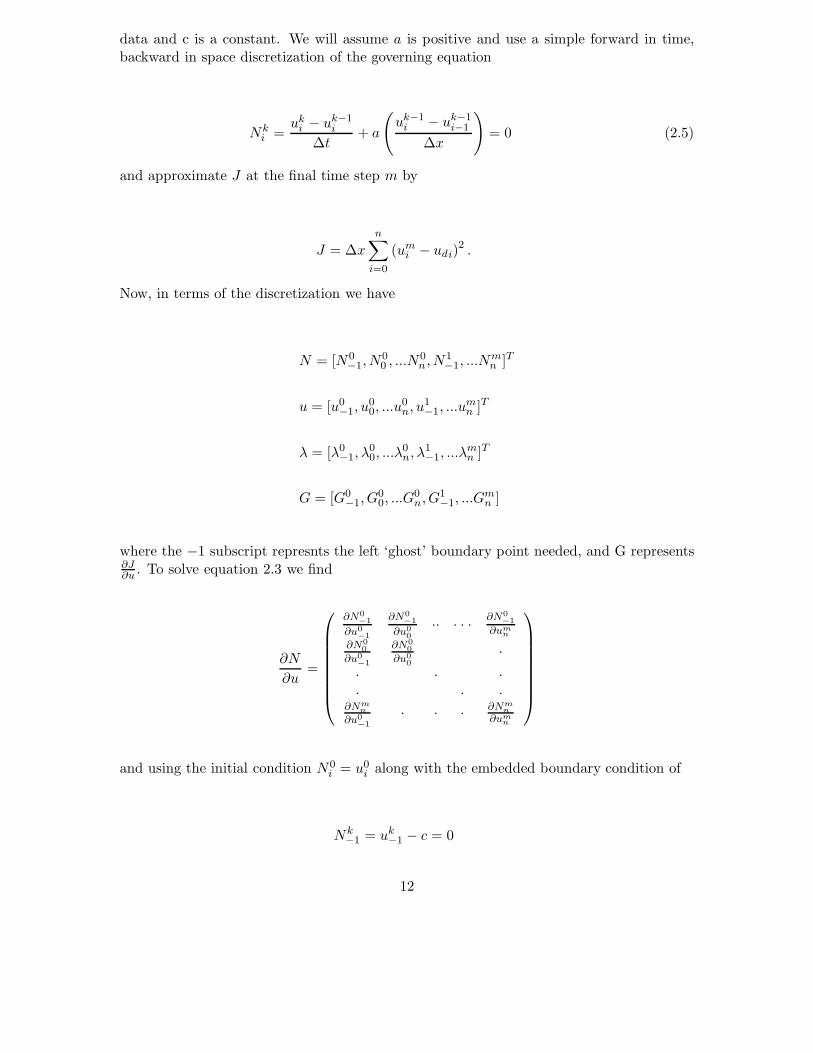
data and c is a constant. We will assume a is positive and use a simple forward in time,backward in space discretization of the governing equation

Nki =

uki − uk−1

i

∆t+ a

(

uk−1i − uk−1

i−1

∆x

)

= 0 (2.5)

and approximate J at the final time step m by

J = ∆x

n∑

i=0

(umi − udi)

2 .

Now, in terms of the discretization we have

N = [N0−1, N

00 , ...N0

n, N1−1, ...N

mn ]T

u = [u0−1, u

00, ...u

0n, u1

−1, ...umn ]T

λ = [λ0−1, λ

00, ...λ

0n, λ1

−1, ...λmn ]T

G = [G0−1, G

00, ...G

0n, G1

−1, ...Gmn ]

where the −1 subscript represnts the left ‘ghost’ boundary point needed, and G represents∂J∂u . To solve equation 2.3 we find

∂N

∂u=

∂N0−1

∂u0−1

∂N0−1

∂u00

·· · · ·∂N0

−1

∂umn

∂N00

∂u0−1

∂N00

∂u00

·

· · ·· · ·

∂Nmn

∂u0−1

· · · ∂Nmn

∂umn

and using the initial condition N0i = u0

i along with the embedded boundary condition of

Nk−1 = uk

−1 − c = 0

12

this becomes

∂N

∂u=

I 0 0 · · 0A11 A21 0 · · 00 A12 A22 ·· · · ·· · · 00 · A1m A2m

where A1k and A2k are (n + 1) × (n + 1) block matrices (with superscripts denoting thetime level) given by

A1k =

0 0 0 · · · 0− a

∆x − 1∆t + a

∆x 0 ·0 − a

∆x − 1∆t + a

∆x ·· · ·· · ·· · ·0 · · · − a

∆x − 1∆t + a

∆x

A2k =

1 · · · 00 1

∆t ·· 1

∆t ·· ·0 · · · 1

∆t

.

For this problem, solving the adjoint turns out to require block solves of sparse structruredmatrices allowing simple direct solvers to be used.

Algorithm 1 Discrete Adjoint Solution, 1-D Linear Advection

A2λm = Gm

for i=m-1 to 1 do

A2λi = Gi − A1T λi+1

end for

λ0 = G0 − A1T λ1

Once the adjoint variable has been found, the gradient can be found as noted in theprevious section by computing 2.4, and the initial condition is updated according to the

13

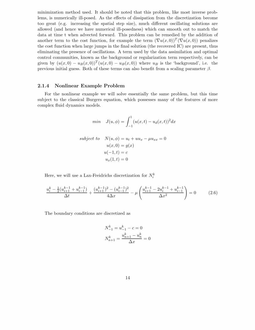
minimization method used. It should be noted that this problem, like most inverse prob-lems, is numerically ill-posed. As the effects of dissipation from the discretization becometoo great (e.g. increasing the spatial step size), much different oscillating solutions areallowed (and hence we have numerical ill-posedness) which can smooth out to match thedata at time t when advected forward. This problem can be remedied by the addition ofanother term to the cost function, for example the term (∇u(x, 0))T (∇u(x, 0)) penalizesthe cost function when large jumps in the final solution (the recovered IC) are present, thuseliminating the presence of oscillations. A term used by the data assimilation and optimalcontrol communities, known as the background or regularization term respectively, can begiven by (u(x, 0) − uB(x, 0))T (u(x, 0) − uB(x, 0)) where uB is the ‘background’, i.e. theprevious initial guess. Both of these terms can also benefit from a scaling parameter β.

2.1.4 Nonlinear Example Problem

For the nonlinear example we will solve essentially the same problem, but this timesubject to the classical Burgers equation, which possesses many of the features of morecomplex fluid dynamics models.

min J(u, φ) =

∫ 1

−1(u(x, t) − ud(x, t))2dx

subject to N(u, φ) = ut + uux − µuxx = 0

u(x, 0) = g(x)

u(−1, t) = c

ux(1, t) = 0

Here, we will use a Lax-Freidrichs discretization for Nki

uki − 1

2(uk−1i+1 + uk−1

i−1 )

∆t+

(uk−1i+1 )2 − (uk−1

i−1 )2

4∆x− µ

(

uk−1i+1 − 2uk−1

i + uk−1i−1

∆x2

)

= 0 (2.6)

The boundary conditions are discretized as

Nk−1 = uk

−1 − c = 0

Nkn+1 =

ukn+1 − uk

n

∆x= 0

14

For this example, the observational data is produced by solving the problem forwardusing the above discretization along with c = 0.5 and g(x) = 0.5 + 0.5e−10·x2

and so thereis no observational error present, i.e. observational data is exact since it is generated fromthe same discretization used in our model with the known solution (the IC g(x)) we aretesting against. For the solution of the inverse problem, poor initial data is chosen so as todemonstrate the ability of the discrete adjoint method, and so we take g(x) = 0.5.

2.1.5 A Matrix Free Representation of the Discrete Adjoint Problem

From the previous example, one could imagine that as the number of dimensions increaseand the governing equations (along with their discretizations) become more sophisticated,the resulting derivative matrix becomes very large, and (despite its sparseness) storage be-comes very undesireable. In the case of realistic computational fluid dynamics problems,the use of traditional sparse solvers may even be out of the question. A few methods havebeen proposed to combat this issue, for example [82] uses a Monte Carlo method to computethe adjoint, as previously mentioned, without storing the Jacobian or the previous solutionstates, but here we will look to take advantage of the inherent structure of the Jacobian.For this reason, we want to seek a matrix free representation that will allow us to computethe gradient. It can easily be seen that the matrix ∂N

∂u will always take on a desireable blocklower triangular shape, and in fact it can always (at worst) take the form

∂N

∂u=

I 0 0 · · 0J1

0 J11 0 · · 0

J20 J2

1 J22 ·

· · · ·· · · 0

Jm0 · · Jm

m−1 Jmm

Where Jki = ∂Nk

∂ui . It is important to note that this notation extends to all dimensions,to be specific, in 1-D

Jki =

∂Nk−1

∂ui−1

∂Nk−1

∂ui0

·· · · · ·∂Nk

−1

∂uin

∂Nk0

∂ui−1

∂Nk0

∂ui0

·

· · ·

·∂Nk

j

∂uij

· · ·∂Nk

n

∂ui−1

· · · · ∂Nkn

∂uin

Then in 2-D, each entry of the sub-Jacobian would become a sub-sub-Jacobian matrix

15

∂Nkj

∂uij

=

∂Nkj,−1

∂uij,−1

∂Nkj,−1

∂uij,0

·· · · · ·∂Nk

j,−1

∂uij,n

∂Nkj,0

∂uij,−1

∂Nkj,0

∂uij,0

·

· · ·

·∂Nk

j,p

∂uij,p

· · ·∂Nk

j,n

∂uij,−1

· · · ·∂Nk

j,n

∂uij,n

and so on. A useful consequence of this setup is that J ii can always be made to be at least

diagonal ‘almost everywhere’, if not the identity matrix. This is dependent on the choiceof boundary conditions, with any non diagonal elements occuring in either the first or lastrow. It is also likely that this will be a banded lower triangular block matrix rather than afull lower triangular matrix depending on the time discretization, and the number of timesteps. For example, the problem in the previous section resulted in a single lower bandwhile the same problem utilizing a leap frog scheme would have two lower bands. Now, inorder to solve 2.3 for λk we have a true back solve since the diagonal blocks are themselvesdiagonal matrices. So here, the solve looks just like a more generalized version of that foundin the example problem.

Algorithm 2 Discrete Adjoint Solution, General Explicit Method

Jmm λm = Gm

for i=m-1 to 1 do

J iiλ

i = Gi −∑m

k=i+1 Jki

Tλk

end for

λ0 = G0 −∑m

k=1 Jk0

Tλk

At this stage, the setup seems (and is) rather nice for simple problems, as the user candetermine the individual sub-Jacobian matrices needed to solve the problem. This can,however, quickly become much more complicated once the governing equations and theirassociated discretizations become more complex, e.g. higher dimensions, systems of equa-tions, higher order methods, etc. So now, we would like to find an easier way to computethe sub-Jacobians. For this we will define the entries of Jk

i in terms of the approximateFrechet derivative so that

Jki ej =

Nk(uij + ǫej) − Nk(ui

j − ǫej)

2ǫ

where ej is the jth column of the identity matrix. So for example in 1-D, the (j, p) entry

16

of Jki is

∂Nkj

∂uip

and we would have

∂Nkj

∂uip

=Nk

j (uip + ǫ) − Nk

j (uip − ǫ)

2ǫ

As an example, to compute Jki

Tfor the discretization 2.5 we could use algorithm 3.

Algorithm 3 Sub-Jacobian Computation

for p=1 to n do

if i=k or i=k+1 then

set temp1(u) = uset temp2(u) = utemp1(ui

p) = uip + ǫ

temp2(uip) = ui

p − ǫfor j=1 to n do

N1 =temp1(uk+1

j )−temp1(ukj )

∆t + a

(

temp1(ukj )−temp1(uk

j−1)

∆x

)

N2 =temp2(uk+1

j )−temp2(ukj )

∆t + a

(

temp2(ukj )−temp2(uk

j−1)

∆x

)

Jki

T(p, j) =

∂Nkj

∂uip

= N1−N22ǫ

end for

else

Jki

T(p, j) =

∂Nkj

∂uip

= 0

end if

end for

So we now have a way to compute the Jacobians required in Algorithm 2 that avoids theerror prone and tedious task of explicitly determining them. This allows for an automatedprocedure capable of solving the adjoint problem for even the most difficult of discretizationmethods. Note that for linear problems, this matrix could be computed once and stored ifdesired, while for the nonlinear case one needs to utilize the solution data from the forwardsolve of the governing equation, and so must be recomputed at every step. Note that un-like automatic differentiation (AD), this method does not require any specific problem byproblem coding, and only relies on the solution data itself. Since AD will not be used here,we will not describe it but will note that it is a popular method due to its high accuracy,and good treatments of this can be found in [50], [37] and [19].

One should take note that in most methods, a vast majority of the Jki matrices will be

0. Indeed, as previously stated it is dependent upon the time discretization. In general, annth order explicit time discretization that utilizes data from only n previous time steps willresult in

17

Jki = 0 if |i − k| > n.

We should also note that in the case of Dirichelet boundary conditions, J ii = I and thus

will not need to be computed. Also note that in a parallel setting, since we only need thematrix vector products Jλ in the computation, we do not need to store J, only the resul-tant vector. So J can be computed, multiplied by λ and be immediately discarded, hencereducing storage and communication costs.

The last bit of information needed is how to choose ǫ. In [61] a similar method is usedin the Jacobian-free Newton Krylov method, and they state the simplest choice for epsilonas (in the translated context of this paper)

ǫ =1

N

N∑

c=1

βuc

Where N is the total number of grid points and β is a constant with value within a feworders of magnitude of machine epsilon.

2.2 Parallel Derivative Free Methods

While adjoint methods work very well for optimization problems with many designvariables, the gradient computation can be problematic for certain classes of problems. Incertain multiphase/multiphysics problems, gradients may be difficult or even impossible tocompute, and hence derivative free methods must be utilized in there place. It is well knownthat derivative free methods, in general, converge very slowly and require a large number offunction evaluations. In PDE constrained optimization, this factor can be very limiting ifthe PDE solution is expensive to compute. For these reasons, we seek a method which cancompute the PDE solves in parallel, allowing us to exploit the rapidly increasing numberof processor cores available to a given architecture. Luckily, most derivative free methodsare parallel in nature and many are embarassingly parallel. We have experimented withthe use of Monte Carlo methods (MC) and genetic algorithms (GA) as global optimizers,but to this point in our research we have primarily focused on the local Multidirectionalsearch method (MDS) [78]. Though originally intended for unconstrained optimization, wefind this method appealing because it is a descent method and was designed for parallelcomputers. Descent type methods are desirable because they reduce the cost function atevery iteration and are guaranteed to converge in many cases. We note that since MDS isa local method, it can become trapped in local extrema, unlike MC or GA.

18

2.2.1 The Multidirectional Search Method

Partly inspired by the Nelder-Mead simplex method, the multidirectional search method(MDS) [17,78,79] is a descent method whose search directions are guaranteed to be linearlyindependent. This method is most appropriate in this setting because it is developed, andideally suited for parallel computation, something that cannot be said of adjoint methods.A key benefit of MDS is that convergence is guaranteed for smooth cost functions [79] andit is more robust than the Nelder-Mead simplex method [78]. A brief description of thegeneral method will now be described.

The multidirectional search method first requires a set of n+1 vertices {vi; i = 0 : n}which form a nondegenerate n-simplex, this can be viewed as the n-dimensional analogueof a triangle, which is in fact a 2-simplex (see figure 2.1). The first step is to computethe value of the cost function for all n+1 vertices, f(v0

i ), and the vertices are then orderedaccording to lowest cost, starting with the 0 subscript. The superscript gives the itera-tion number. The n edges connecting the best vertex to the rest provide the set of searchdirections, which are linearly independent. A reflection step is then taken, in which wefind v1

i = 2v00 − v0

i and then calculate f(v1i ). If a new minimum value is found, then an

expansion step is taken to see if an even better point can be found. This is calculated asv0ei

= (1 − µ)v00 + µv1

i , and if f(v0ei

) < f(v1i ), then v1

i = v0ei

. If, however, we do not obtaina better point after the reflection step, then we instead perform a contraction in a similarmanner, vk+1

i = (1 + θ)vk0 − θvk+1

i . The vertices are then reordered and we move on to thenext iteration and repeat the process. The algorithm as described in [79] is given in alg.2.2.1.

1

2 3

2-Simplex

1

2

3

3-Simplex

4

Figure 2.1: 2-Simplex (Left): A two dimensional triangle made by connecting 3vertices. 3-Simplex (Right): A 3 dimensional tetrahedron made of triangles byconnecting 4 vertices

A question arises here of how MDS may be applied to PDE constrained optimization.In the context of the 1-D data assimilation problems of this chapter, suppose we have a

19

Algorithm 4 The Multidirectional Search Algorithm of Torczon [79].

Given an initial simplex S0 with vertices {u00, u

01, ..., u

0n}, µ ∈ (1,+∞) and θ ∈ (0, 1)

for i = 0 to n do

calculate f(uki )

end for

k = 0// outer while loopwhile stopping criterion is not satisfied do

// find a new best vertexj = mini{f(uk

i ) : i = 0, ..., n}swap uk

j and uk0

repeat

Check stopping criterion// rotation stepfor i = 1 to n do

rki = uk

0 − (uki − uk

0)calculate f(rk

i )end for

eki = uk

0 − µ(uki − uk

0)replaced = (min{f(rk

i ) : i = 1, ..., n} < f(uk0))

if replaced then

// expansion stepfor i = 1 to n do

eki = uk

0 − µ(uki − uk

0)calculate f(ek

i )end for

if min{f(eki ) : i = 1, ..., n} < min{f(rk

i ) : i = 1, ..., n} then

// accept expansionuk

i = eki for i = 1, ..., n

else

// accept rotationuk

i = rki for i = 1, ..., n

end if

else

// contraction stepfor i = 1 to n do

cki = uk

0 + θ(uki − uk

0)calculate f(ck

i )end for

replaced = (min{f(cki ) : i = 1, ..., n} < f(uk

0))// accept contractionuk

i = cki for i = 1, ..., n

end if

until replacedk = k + 1

end while

20

candidate solution for the recovered IC in vector form. In this scenario we can create asimplex by augmenting the solution with a set of n linearly independent alternate solutionsin the form of a scaled identity matrix, and use a multidirectional search on this set inorder to find a single optimal solution. We note that simplex-type methods such as MDSare not typically used for problems with a large number of degrees of freedom, or whatwe would consider here to be design variables. For algorithm 2.2.1, each additional designvariable introduced into the problem requires an additional flow solve computation at eachcost function evaluation step. For this reason it is important to note here that we intendto use MDS in a design code for problems with a small number of design variables, whichwill be described later.

2.2.2 A Multigriding Strategy for the Multidirectional Search Method

While we find MDS to be a promising derivative free method with which to carry outour simulation based design goals, we would also like to find ways in which to reducethe number of iterations required to achieve convergence, as each iteration requires a flowsolve which can become very costly. One such way to accelerate convergence that hasbeen used on gradient based methods [52, 58] is to use a multigriding strategy. Multigridmethods [10] are well known for accelerating the convergence rates of PDE systems on finegrids when the PDE system’s qualitative solution features can be captured using coarselevel grids. Multigrid methods should also be effective on nonlinear problems [10] and havea solid research base in CFD applications [20, 38]. Since our proposed MDS algorithm isdependent on such PDE systems, and since success in reducing the number of iterationsto convergence for gradient based methods has been achieved by employing multigridingstrategies [52, 58], it seems logical to attempt to accelerate our MDS algorithm as well byutilizing a multigriding strategy. In order to test this strategy, we have devolped two MGalgorithms for the MDS method (MGMDS) using the MG cycle strategies of figure 2.2. Thefirst uses a V-cycle strategy where one starts with a fine grid approximation to the solution,this method is demonstrated by algorithm 5. As an alternative strategy, we have also usedan MGMDS algorithm which starts with a coarse grid approximation using what is referedto as a full multigrid (FMG) cycle, which is described in algorithm 6. We note that whilealgorithms 5 and 6 are both set up for multiple MG cycles, we currently have no coarse gridcorrection mechanism and so should be restricted to a single cycle in practice.

2.3 Numerical Results and Discussion

Presented in this section are some numerical findings based on the solution of both alinear and nonlinear test problem formulated using the discrete adjoint method and boththe traditional MDS method of Torczon [78] and the novel MGMDS method described inalgorithms 5 and 6. For the linear case, the 1-D advection problem is solved, while forthe nonlinear case, a similar 1-D problem is posed utilizing Burgers equation in place ofthe advection equation. Comparisons for the two formulations of each problem are made.We note that in the discrete adjoint case, the solutions utilizing the stored matrix and thecomputed matrix free versions of the flow Jacobian are identical. We have also found that for

21

V−Cycle FMG−Cycle

h h

2h

4h

2h

4h

Figure 2.2: Multigrid cycling schemes tested in this work include the V-Cycle andthe full multigrid cycle (FMG).

Algorithm 5 A Multigrid-Multidirectional Search Algorithm, V-Cycle Strategy

Given a fine level grid XN and an initial simplex SN of solutions on XN , {u00, u

01, ..., u

0n},

choose an expansion factor µ ∈ (1,+∞) and a contraction factor θ ∈ (0, 1).while cost > tol and cycles < maxcycles do

k = N// begin v-cyclerepeat

Call MDS(Sk,Xk, µ, θ,maxiterates)restrict S,X, → k=k-1

until k=0Call MDS(S0,X0, µ, θ, bottomiterates)repeat

Call MDS(Sk,Xk, µ, θ,maxiterates)prolong S,X, → k=k+1

until k = N// end v-cycle

end while

if cost > tol then

// MG cycles complete, begin final MDS iterationsCall MDS(SN ,XN , µ, θ, f inaliterates)

end if

22

Algorithm 6 A Multigrid-Multidirectional Search Algorithm, FMG Strategy

Given a fine level grid XN and an initial simplex SN of solutions on XN , {u00, u

01, ..., u

0n},

choose an expansion factor µ ∈ (1,+∞) and a contraction factor θ ∈ (0, 1).while cost > tol and cycles < maxcycles do

Restrict X,S to the coarsest grid → k=0Call MDS(S0,X0, µ, θ,maxiterates)ℓ = 1repeat

for i = 1 to ℓ do

prolong X,S → k=k+1Call MDS(Sk,Xk, µ, θ,maxiterates)

end for

for i = ℓ to 1 do

restrict X,S → k=k-1Call MDS(Sk,Xk, µ, θ,maxiterates)

end for

ℓ = ℓ + 1until ℓ = Nfor i = 1 to N do

prolong X,S → k=k+1Call MDS(Sk,Xk, µ, θ,maxiterates)

end for

end while

if cost > tol then

Call MDS(SN ,XN , µ, θ, f inaliterates)end if

23

these test cases, the use of the penalty term (∇u)T (∇u) and the traditional background, orregularization term in the cost function give essentially the same result, producing solutionerrors that are consistently within the same order of magnitude.

2.3.1 Linear Advection Problem

For the linear advection example, we demonstrate a recovery of the initial conditionsin a 1-D data assimilation problem whose solution possesses a steep gradient, and startingwith a poor initial guess. The problem is

min J(u, φ) =

∫ 1

−1(u(x, T ) − ud(x, T ))2dx + β(∇u(x, 0))T (∇u(x, 0))

subject to N(u, φ) = ut + aux = 0

The data, ud, is generated by advecting a step function IC forward using the samediscretization as for the problem solution. The discretization method is again the forwardEuler method, the exact IC we wish to recover is

g(x) =

{

1.0 −0.5 < x < 00.5 Otherwise

.

We start with an initial guess of g(x) = 0. The plots in figures 2.3 to 2.10 show the actualdata, and the solution u after convergence. The plots to the left are at time t=0, and showthe exact IC we wish to recover (solid line), and the IC recovered using the discrete adjointand MDS methods (dash dot line). The plots on the right are at time t=1.0, and show theadvected solutions from these starting IC’s. These plots all have a value of β = 1.0 for thecost function.

2.3.2 Nonlinear Burgers Equation Problem

For the Burgers problem, we will again use a single set of final end time observationsand a poor initial guess of g(x) = 0.5, with the fixed parameters N=96, dt=0.005, beta= 1.0. To demonstrate the effects of nonlinear features on the solution, we have solvedthis problem for various end times. The first figure 2.11 shows that the IC is recovered towithin a pretty close range of the exact IC used, but only after a very short time. As timeprogresses, however, one can see that the recovered initial condition becomes progressivelyworse to the point of showing little resemblance to the correct solution as in figure 2.19.To remedy this, additional time observations must be provided. Note that increasing thenumber of observations in time directly leads to improved solution quality for nonlinear

24

X

U,d

ata

-1 -0.5 0 0.5 1

0.2

0.3

0.4

0.5

0.6

0.7

0.8

0.9

1

Ud

X

U,d

ata

-1 -0.5 0 0.5 1

0.2

0.3

0.4

0.5

0.6

0.7

0.8

0.9

1

Udata

Figure 2.3: Adjoint solution for linear advection problem. Left: Recovered IC for64 grid points (U) versus exact IC (data). Right: Comparison of the advectedsolutions. β = 1.0, ∆x = 1

32 , ∆t = 0.01. Requires 200 iterations for convergenceand runs in 1.945 seconds on a single CPU core.

x

U,d

ata

-1 -0.5 0 0.5 1

0.2

0.4

0.6

0.8

1

dataU

x

U,d

ata

-1 -0.5 0 0.5 1

0.2

0.4

0.6

0.8

1

dataU

Figure 2.4: MDS solution for linear advection problem. Left: Recovered IC for64 grid points (U) versus exact IC (data). Right: Comparison of the advectedsolutions. β = 1.0, ∆x = 1

32 , ∆t = 0.01. Requires 8470 iterations for convergenceand runs in 50.183 seconds on four CPU cores.

25

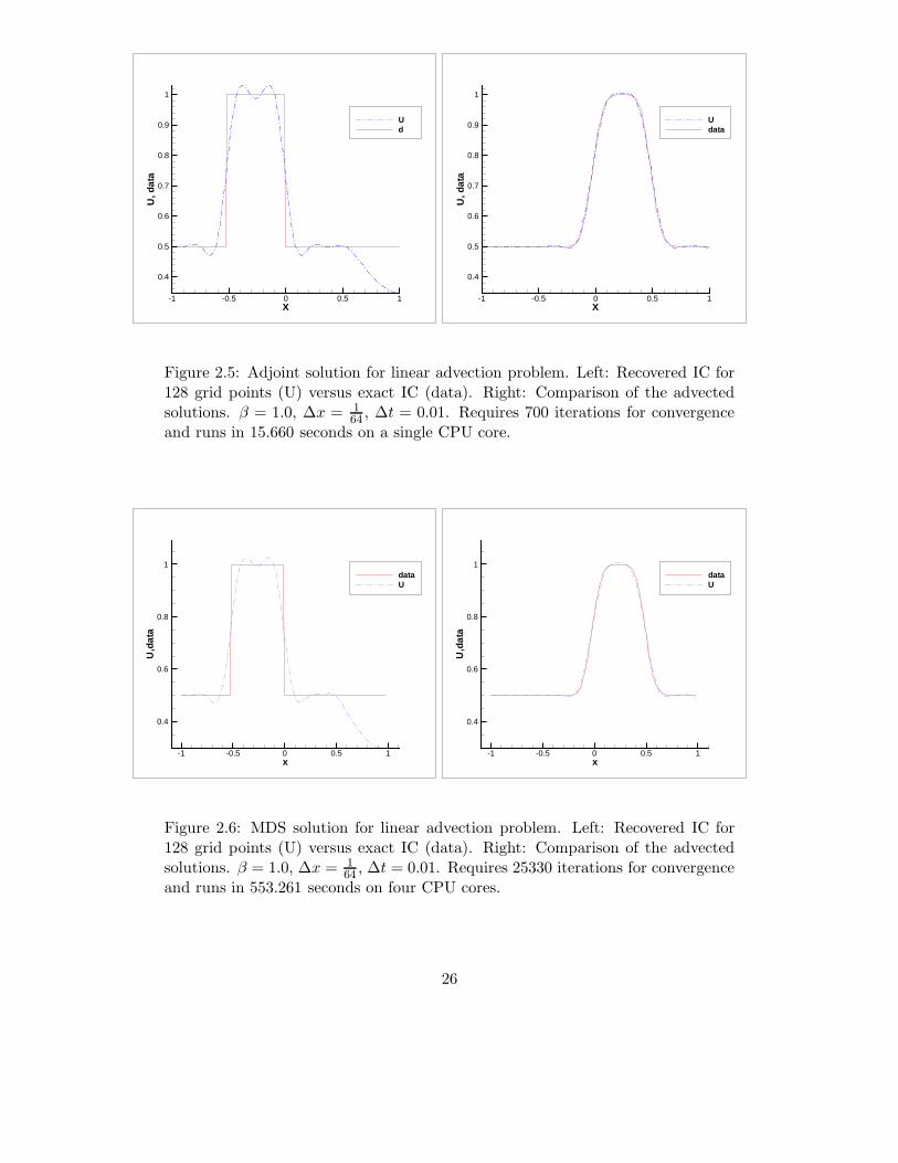
X

U,d

ata

-1 -0.5 0 0.5 1

0.4

0.5

0.6

0.7

0.8

0.9

1

Ud

X

U,d

ata

-1 -0.5 0 0.5 1

0.4

0.5

0.6

0.7

0.8

0.9

1

Udata



x

U,d

ata

-1 -0.5 0 0.5 1

0.4

0.6

0.8

1dataU

x

U,d

ata

-1 -0.5 0 0.5 1

0.4

0.6

0.8

1dataU



26

X

U,d

ata

-1 -0.5 0 0.5 1

0.4

0.5

0.6

0.7

0.8

0.9

1

Ud

X

U,d

ata

-1 -0.5 0 0.5 1

0.4

0.5

0.6

0.7

0.8

0.9

1

Udata



x

U,d

ata

-1 -0.5 0 0.5 1

0.4

0.6

0.8

1

dataU

x

U,d

ata

-1 -0.5 0 0.5 1

0.4

0.6

0.8

1

dataU



27

X

U,d

ata

-1 -0.5 0 0.5 10.4

0.5

0.6

0.7

0.8

0.9

1

Ud

X

U,d

ata

-1 -0.5 0 0.5 10.4

0.5

0.6

0.7

0.8

0.9

1

Udata



x

U,d

ata

-1 -0.5 0 0.5 1

0.4

0.6

0.8

1

dataU

x

U,d

ata

-1 -0.5 0 0.5 1

0.4

0.6

0.8

1

dataU



28

problems. This is important, as it is known that increasing the number of observationaldata points for a single time does not have a major impact [26], but here we see that in-creasing the number of time observations indeed does.

X

U,d

ata

-1 -0.5 0 0.5 1

0.2

0.3

0.4

0.5

0.6

0.7

0.8

0.9

1

Udata

X

U,d

ata

-1 -0.5 0 0.5 1

0.2

0.3

0.4

0.5

0.6

0.7

0.8

0.9

1

Udata

Figure 2.11: Adjoint solution for non-linear Burger’s equation problem. Left:Recovered IC (U) versus exact IC (data), t=0.05. Right: Comparison of the finalsolutions. β = 1.0, ∆x = 1

48 , ∆t = 0.005, µ = 0.001. Requires 200 iterations forconvergence and runs in 4.339 seconds on a single CPU core.

2.3.3 Multigrid-Multidirectional Search Strategies

Employing the multigriding strategies of algorithms 5 and 6 have proven effective atsubstantially reducing the number of iterations required for convergence of both the linearadvection and the nonlinear Burger’s data assimilation problems in many scenarios. For thelinear advection problem, we have found that both the v-cycle and FMG cycles produce nearoptimal results by using approximately 300 fixed iterations of the MDS solver at each level.While we have seen good speedup by employing multigriding strategies, one can see from thefigures that the quality of the converged solution does suffer slightly, and we attribute thisto the lack of a correction step in our algorithm. One method we have employed to try andsmooth out these small errors that eminate from the use of a multigriding strategy is to usea weighted average of the fine grid solutions. To accomplish this, we take a weighted averageof the solution everytime we arrive at a fine grid in the MG cycle, i.e. U = θU +(1− θ)Uold

for a θ ∈ (0, 1). This has shown to be useful in smoothing out the solution of the linearadvection problem when more than 1 FMG cycle is used as seen in figure 2.25, but at thecost of added sppedup as seen in table 2.3.

29

x

U,d

ata

-1 -0.5 0 0.5 1

0.4

0.5

0.6

0.7

0.8

0.9

1

dataU

x

U,d

ata

-1 -0.5 0 0.5 1

0.4

0.5

0.6

0.7

0.8

0.9

1

dataU

Figure 2.12: MDS solution for non-linear Burger’s equation problem. Left: Re-covered IC (U) versus exact IC (data), t=0.05. Right: Comparison of the finalsolutions. β = 1.0, ∆x = 1

48 , ∆t = 0.005, µ = 0.001. Requires 720 iterations forconvergence and runs in 2.763 seconds on four CPU cores.

X

U,d

ata

-1 -0.5 0 0.5 1

0.2

0.3

0.4

0.5

0.6

0.7

0.8

0.9

1

Udata

X

U,d

ata

-1 -0.5 0 0.5 1

0.2

0.3

0.4

0.5

0.6

0.7

0.8

0.9

1

Udata



30

x

U,d

ata

-1 -0.5 0 0.5 1

0.4

0.5

0.6

0.7

0.8

0.9

1

dataU

x

U,d

ata

-1 -0.5 0 0.5 1

0.4

0.5

0.6

0.7

0.8

0.9

1

dataU



X

U,d

ata

-1 -0.5 0 0.5 1

0.2

0.3

0.4

0.5

0.6

0.7

0.8

0.9

1

Udata

X

U,d

ata

-1 -0.5 0 0.5 1

0.2

0.3

0.4

0.5

0.6

0.7

0.8

0.9

1

Udata



31

x

U,d

ata

-1 -0.5 0 0.5 1

0.4

0.5

0.6

0.7

0.8

0.9

1

dataU

x

U,d

ata

-1 -0.5 0 0.5 1

0.4

0.5

0.6

0.7

0.8

0.9

1

dataU



X

U,d

ata

-1 -0.5 0 0.5 1

0.2

0.3

0.4

0.5

0.6

0.7

0.8

0.9

1

Udata

X

U,d

ata

-1 -0.5 0 0.5 1

0.2

0.3

0.4

0.5

0.6

0.7

0.8

0.9

1

Udata



32

x

U,d

ata

-1 -0.5 0 0.5 1

0.4

0.5

0.6

0.7

0.8

0.9

1

dataU

x

U,d

ata

-1 -0.5 0 0.5 1

0.4

0.5

0.6

0.7

0.8

0.9

1

dataU



X

U,d

ata

-1 -0.5 0 0.5 1

0.2

0.3

0.4

0.5

0.6

0.7

0.8

0.9

1

Udata

X

U,d

ata

-1 -0.5 0 0.5 1

0.2

0.3

0.4

0.5

0.6

0.7

0.8

0.9

1

Udata



33

x

U,d

ata

-1 -0.5 0 0.5 1

0.4

0.5

0.6

0.7

0.8

0.9

1

dataU

x

U,d

ata

-1 -0.5 0 0.5 1

0.4

0.5

0.6

0.7

0.8

0.9

1

dataU



Table 2.1: V-cycle multigriding strategy applied to the multidirectional searchmethod on the 1D linear advection data assimiliation problem for N=400 gridpoints. V-cycles utilize 300 iterations at each grid level, and the final number ofMDS iterations required for the solver to converge are also listed. Time representsuser time on four processor cores. Baseline time for the original MDS algorithmis 17977 seconds.

V-Cycles (maxcycles) Final MDS Iterations (finaliterates) Time (s) Speedup

1 24740 21968 0.82X2 10350 10586 1.70X3 8360 9554 1.88X4 10100 11691 1.54X

34

Table 2.2: FMG multigriding strategy applied to the multidirectional searchmethod on the 1D linear advection data assimiliation problem for N=400 gridpoints. The FMG cycle utilizes between 200 and 400 iterations at each grid level,the final number of MDS iterations required for the solver to converge are alsolisted. Time represents user time on four processor cores. Baseline time for theoriginal MDS algorithm is 17977 seconds.

maxiterates Final MDS Iterations (finaliterates) Time (s) Speedup

200 9280 8911 2.02X250 7040 7179 2.50X300 2260 3279 5.48X350 5780 6381 2.82X

x

U,d

ata

-1 -0.5 0 0.5 1

0.4

0.5

0.6

0.7

0.8

0.9

1dataU

x

U,d

ata

-1 -0.5 0 0.5 1

0.4

0.5

0.6

0.7

0.8

0.9

1dataU

Figure 2.21: MGMDS solution for linear advection problem using an FMG cyclewith 200 iterations at each level. Left: Recovered IC for 400 grid points (U) versusexact IC (data). Right: Comparison of the advected solutions. β = 1.0, ∆x = 1

200 ,∆t = 0.01.

35

x

U,d

ata

-1 -0.5 0 0.5 1

0.4

0.5

0.6

0.7

0.8

0.9

1dataU

x

U,d

ata

-1 -0.5 0 0.5 1

0.4

0.5

0.6

0.7

0.8

0.9

1dataU

Figure 2.22: MGMDS solution for linear advection problem using an FMG cyclewith 300 iterations at each level. Left: Recovered IC for 400 grid points (U) versusexact IC (data). Right: Comparison of the advected solutions. β = 1.0, ∆x = 1

200 ,∆t = 0.01.

x

U,d

ata

-1 -0.5 0 0.5 1

0.5

0.6

0.7

0.8

0.9

1dataU

x

U,d

ata

-1 -0.5 0 0.5 1

0.5

0.6

0.7

0.8

0.9

1dataU

Figure 2.23: MGMDS solution for linear advection problem using 2 V-cycles with300 iterations at each level. Left: Recovered IC for 400 grid points (U) versusexact IC (data). Right: Comparison of the advected solutions. β = 1.0, ∆x = 1

200 ,∆t = 0.01. Requires 2 V-cycles plus 10350 final MDS iterations for convergenceand runs in 2515.487 seconds on four CPU cores.

36

x

U,d

ata

-1 -0.5 0 0.5 1

0.4

0.5

0.6

0.7

0.8

0.9

1

dataU

x

U,d

ata

-1 -0.5 0 0.5 1

0.4

0.5

0.6

0.7

0.8

0.9

1

dataU

Figure 2.24: MGMDS solution for nonlinear Burger’s problem using an FMGcycle. Left: Recovered IC for 256 grid points (U) versus exact IC (data). Right:Comparison of the advected solutions. β = 1.0, ∆x = 1

48 , ∆t = 0.005, µ = 0.001.

Table 2.3: FMG multigriding strategy applied to the multidirectional searchmethod on the 1D linear advection data assimiliation problem for N=400 gridpoints, and employing a weighted averaging of the fine grid solutions, θ = 0.5.The FMG cycle utilizes 300 iterations at each grid level, the final number of MDSiterations required for the solver to converge are also listed. Time represents usertime on four processor cores. Baseline time for the original MDS algorithm is17977 seconds.

FMG Cycles Final MDS Iterations Time (s) Speedup

1 4350 4863 3.70X2 4460 5760 3.12X3 5370 7308 2.46X4 6630 9152 1.96X

37

x

U,d

ata

-1 -0.5 0 0.5 1

0.5

0.6

0.7

0.8

0.9

1 dataU

x

U,d

ata

-1 -0.5 0 0.5 1

0.5

0.6

0.7

0.8

0.9

1dataU

x

U,d

ata

-1 -0.5 0 0.5 1

0.5

0.6

0.7

0.8

0.9

1dataU

x

IC,u

(1)

-1 -0.5 0 0.5 1

0.5

0.6

0.7

0.8

0.9

1

Figure 2.25: MGMDS IC recovery for a 1D linear advection data assimilationproblem using an FMG cycle employing a weighted averaging of the fine gridsolution. Using more than one FMG cycle results in a smoothing effect on thesolution data. Top Left: 1 FMG cycle. Top Right: 2 FMG cycles. Bottom Left:3 FMG cycles. Bottom Right: 4 FMG cycles. β = 1.0, ∆x = 1

200 , ∆t = 0.01 forall figures.

38

2.3.4 Discussion of Numerical Results

We should note that the numerical experiments carried out here were under conditionsfar from ideal. Usually, a good starting estimate along with more available data (i.e. datacollected at multiple time intervals) is used for the problem solution in data assimilationproblems, but here we have purposely used poor initial guesses along with limited data.It can be seen that for linear problems, the adjoint method works very well and is able torecover a difficult initial condition possessing steep gradients with ease using only a singleset of observed solutions, and that as the computational grid is resolved the error tendstowards zero. The MDS algorithm also works well for the linear advection problem, pro-ducing qualitative solutions very similar to those of the adjoint method despite the largenumber of design variables.

The adjoint method does not work as well on the nonlinear Burgers problem, as poorinitial guesses will produce poorer and poorer solutions as the solution is carried out furtherand further in time. This is due to the nonlinear features, and in this scenario the useof data for multiple times should be used to correct this problem. The figures provided(2.26, 2.27, 2.28) demonstrate how increasing the number of observations leads to improvedsolutions for nonlinear problems. We note that many observations are typically used indata assimilation problems and that errors resulting from non-linear model features are wellknown, though those produced by data assimilation tend to be lower than those producedby other predictive modeling methods, see for example [6]. The MDS method works verywell on the nonlinear Burger’s problem even in the absence of additional observational dataas can be seen by figures 2.11 - 2.20.

X

U,d

ata

-1 -0.5 0 0.5 1

0.2

0.3

0.4

0.5

0.6

0.7

0.8

0.9

1

Udata

X

U,d

ata

-1 -0.5 0 0.5 1

0.2

0.3

0.4

0.5

0.6

0.7

0.8

0.9

1

Udata

Figure 2.26: Adjoint nonlinear IC Recovery, 5 observations. Left: Recovered IC(U) versus exact IC (data), t=0.5. Right: Comparison of the final solutions.β = 1.0, ∆x = 1

48 , ∆t = 0.005, µ = 0.001.

We would like to compare how well the multidirectional search with and without a

39

X

U,d

ata

-1 -0.5 0 0.5 1

0.2

0.3

0.4

0.5

0.6

0.7

0.8

0.9

1

Udata

X

U,d

ata

-1 -0.5 0 0.5 1

0.2

0.3

0.4

0.5

0.6

0.7

0.8

0.9

1

Udata

Figure 2.27: Adjoint nonlinear IC Recovery, 10 observations. Left: RecoveredIC (U) versus exact IC (data), t=0.5. Right: Comparison of the final solutions.β = 1.0, ∆x = 1

48 , ∆t = 0.005, µ = 0.001.

X

U,d

ata

-1 -0.5 0 0.5 1

0.2

0.3

0.4

0.5

0.6

0.7

0.8

0.9

1

Udata

X

U,d

ata

-1 -0.5 0 0.5 1

0.2

0.3

0.4

0.5

0.6

0.7

0.8

0.9

1

Udata

Figure 2.28: Adjoint nonlinear IC Recovery, 20 observations. Left: RecoveredIC (U) versus exact IC (data), t=0.5. Right: Comparison of the final solutions.β = 1.0, ∆x = 1

48 , ∆t = 0.005, µ = 0.001.

40

multigriding strategy compares to the adjoint method for the numerical examples given.While it is very clear that the discrete adjoint method is substantially faster than MDSin a sequential setting, we wish to show that in the presence of abundant processors theMDS method can compete on par with the discrete adjoint method on a single core. Forthis purpose we will compare the linear advection problem with N=400 grid points sinceit produced the most accurate results for all methods involved here. For this problem, thediscrete adjoint code converged in 200 iterations and took 57.158 seconds to complete. Incontrast, it took the MDS method 20690 iterations to converge and 16970 seconds on a singlecore. In parallel, the same MDS code ran in 4694 seconds, giving a parallel efficiency ofabout 0.9 on a shared memory system. We note that the parallel efficiency was higher in allother cases, and almost linear for the N=256 case, so we feel that 0.9 is a safe estimate to usefor this hypothetical exercise. The MDS method can be considered ‘embarassingly parallel’on up to N+1 processors since this is how many parallel flow solves can be done at once. So,if we were to theoretically have 401 processors on a shared memory system, then this codewould take approximately 47 seconds (=16970.342/(401*0.9)) to run (a little faster than theadjoint code), and using this parallel efficiency we would require approximately 330 cores tomatch the speed of the adjoint code. The MGMDS code is much more promising. Considerusing the FMG cycle with 300 iterations at each grid level, then the estimated parallelefficiency is 0.94 and takes 3090 seconds on a single core. In this scenario we would onlyneed about 58 cores to match the speed of the adjoint method, and with 401 cores wouldbe 7X faster than the adjoint method. We note that our discrete adjoint code could alsobenefit somewhat from parallelization, but the underlying algorithm is inherently sequentialand the parallel efficiency would likely be very low.

41

CHAPTER 3

CFD CODE ACCELERATION

In this chapter we will discuss some approaches that have been taken in order to acceleratetwo CFD codes, the NASA FUN3D code and the coupled level-set and volume-of-fluid(CLSVOF) code for incompressible multiphase flows. While we have primarily focusedon the use of add on GPU hardware for accelerating CFD codes, we will also discussan improved pressure projection algorithm for adaptive mesh refinement (AMR) that wehave recently developed. This new algorithm based on Tatebe’s multigrid preconditionedconjugate gradient method (MGPCG) [76] substantially reduces the computational effortrequired by the projection step when compared to MG AMR solvers, and also improves thescalability of the CLSVOF code by avoiding a ‘domain decomposition penalty’.

3.1 Graphics Processors and Hybrid Computing

Architectures

Modern graphics processors along with languages such as the breakthrough ’ComputeUnified Device Architecture’ (CUDA) [14] and OpenCL to program them has allowed forscientific computations on distributed computers to benefit from an additional level of finegrain parallelism at the node level. When attempting to develop an accelerated version of alarge parallel CFD code, several challenges present themselves. To start with, these codeshave already been highly optimized for parallel computation and so the biggest possible gainsmay have already been accounted for. One must look beyond coarse grain parallelism (e.g.,dividing a grid into blocks and distributing them over multiple CPU cores) and seek finegrained data parallel tasks which can be ported to the GPU. If these opportunities exist fora large scale code, it has the potential to benefit from an added level of parallelism. Parallelcodes also must employ frequent MPI communications, which when used in an acceleratorenvironment will implicitly invoke expensive GPU-CPU data transfers. Scalability is alsoa big issue for all production level CFD codes. With the rising number of CPU cores perprocessor coupled with the rising cost and power consumption of an individual GPU, it isnot likely that future large scale hybrid architectures will be able to maintain a 1:1 or betterratio of GPUs to CPU cores. The new availability of concurrent kernel execution allowsmultiple cores to share a single GPU. This feature should allow hybrid codes to scale onsystems with a GPU to CPU ratio below 1. This feature does come at a price though, asincreasing the number of CPU threads which simultaneously share a single GPU puts added

42

demand on the available memory and could put additional strains on other resources forlarge kernels. In addition to these challenges, the unstructured solver of FUN3D is hinderedby the unavoidable constraint of out-of-order memory access patterns, which can cause verypoor performance on a GPU. In this chapter we will describe the CLSVOF and FUN3Dcodes, and detail the various strategies we have employed to accelerate them.

3.2 The Coupled Level-Set and Volume-of-Fluid Method

We will consider the following incompressible Navier-Stokes equations for multiphaseflow [73]:

ρ(φ)(~ut + ~u · ∇~u) = −∇p + ∇ · µ(φ)∇D − γκ(φ)∇H(φ) + ρ~g.

∇ · ~u = 0.

where ρ(φ) is the density, µ(φ) is the viscosity, ~u is the velocity, D is the rate of deformationtensor, p is the pressure, κ(φ) is the curvature, ~g is the gravitational forces, and H(φ) isthe Heaviside function.

In the level set approach, the set of points,

Γ = {(x, y, z)|φ(x, y, z, t) = 0},

represents the air/water interface Γ at time t. For single-valued surfaces the points satisfyingz = ζ(x, y, t) represents the zero level set of φ(x, y, z, t). The advantage of using φ(x, y, z, t)is that multi-valued surfaces are handled naturally. Also, the level set representation of aninterface does not break down if the interface changes topology: e.g. if an interface break-upoccurs or if surfaces reconnect. The equation governing the level set function is given by,

φt + ~u · ∇φ = 0.

In order to increase the accuracy for simulating multi-phase flows, we have developedadaptive mesh refinement (AMR) level set methodology in order to dynamically place gridpoints in the vicinity of the air/water interface [18,70–72].

The key component of this work considers the solution of the pressure projection equa-tion,

∇ ·1

ρ∇p = ∇ · ~u∗, (3.1)

where ~u∗ is an intermediate velocity field resulting from a standard “projection method”splitting scheme, and the density ρ is represented by both liquid and gas phases

ρ = ρLH(θ) + ρG(1 − H(θ)).

The discretization utilizes the level set function such that ρ is a function of φ and

43

ρi+1/2,j(φ) = ρLθi+1/2,j + ρG(1 − θi+1/2,j)

where θi+1/2,j is a height fraction,

θi+1/2,j =φ+

i,j + φ+i,j+1

|φi,j| + |φi,j+1|

and φ+ = max(φ, 0). The spatial discretization of eqn. 3.1 utilizes cell centered values for pwith corresponding values at the cell faces for ρ such as in the example 1D discretization 3.3.We note that the use of first order boundary conditions results in a symmetric discretizationmatrix [53,54]. We will primarily be concerned with solving equation 3.1.

3.2.1 Solution of the Pressure Poisson Equation

The numerical simulation of incompressible fluid flows consisting of multiple phases withlarge density variations (such as in liquid-gas scenarios) can present significant challenges,particularly in the solution of the pressure projection step. The phase density ρ is repre-sented in liquid and gas phases by ρ = ρLH(φ) + ρG(1−H(φ)), where H(φ) is a Heavisidefunction equal to 1 in liquid and 0 in gas. The rate of convergence of the iterative solutionof the pressure Poisson equation

∇ ·1

ρ∇p = F (3.2)

is retarded if ρL

ρG>> 1 because the resulting discretization matrix is very poorly conditioned.

Consider the 1D discretization of eqn. 3.2

1ρ

i+12

pi+1−pi

∆x − 1ρ

i− 12

pi−pi−1

∆x

∆x= Fi, (3.3)

where ρi+ 1

2

= 1 in a first phase and α in a second phase, then the condition number of the

corresponding discretization matrix becomes larger as the density ratio increases as seen intable 3.1. Though we have seen that the condition number is sensitive to the density ratio,we have found that the condition number is not necessarily sensitive to the problem geom-etry as seen in figure 3.2, where all illustrated geometries produce a discretization matrixwhose condition number is of the same order of magnitude.

Significant steps in reducing the solution time of the pressure projection step for theseproblems have come from separate sources. The development of adaptive mesh refinement[7, 8, 34, 72] (AMR) has allowed for a reduction in the number of required computationalgrid points when used in conjuction with a method such as multigrid (MG). Unstructuredgrid coarsening strategies have been implemented to allow for MG solutions of the Poisson

44

p0

p p p p p p1 2 3 54 6

ρ ρ ρ ρ ρ ρ ρ ρ−1/2 1/2 3/2 5/2 7/2 9/2 11/2 13/2

N=7

Figure 3.1: Example 1D discretization for the pressure Poisson equation

Table 3.1: In multiphase flows, the condition number of the discretization matrixfor eqn. 3.2 grows with the density ratio. In this table, the condition numberis calculated for the discretization matrix of a 1D two phase flow in the domain[0, 1] following eqn. 3.3, and with the phase interface occurring at x = 0.25. Theexample flow has a density of 1 in the first phase on the interval [0, 0.25) and α ina second phase on the interval (0.25, 1]. Values represent a discretization with 256grid points and were calculated in MATLAB using the built in condition numberfunction cond().

α 1 10−1 10−2 10−3 10−4 10−5

Density Ratio 1 10 102 103 104 105

Condition # 205 1.2 x 103 1.2 x 104 1.2 x 105 1.2 x 106 1.2 x 107

ρ=1

ρ=0.001

ρ=1

ρ=0.001

ρ=0.001

ρ=1

ρ=0.001

Figure 3.2: The condition number of the discretization matrix is not as sensitiveto the problem geometry as it is to the density ratio. The corresponding conditionnumbers for these figures are 6,132,300 (left), 1,861,000 (middle) and 2,548,900(right) using a 2D version of discretization eqn. 3.3 on a 64 x 64 grid.

45

equation in unstructured applications [81]. Alternatively, on uniform grids, MG has beenused to form the preconditioning matrix for the preconditioned conjugate gradient (PCG)method. The multigrid preconditioned conjugate gradient method (MGPCG) was firstintroduced by Tatebe [76] who showed that poorly conditioned problems could be solved12 times faster using MGPCG instead of MG, and 5 times faster than incomplete LUpreconditioned CG (ILU-PCG). In our previous work [71] we developed a pressure solveron an adaptive hierarchy of grids using a combination of MG and MGPCG. The MGPCG“smoother” was applied a single level at a time. We have discovered though, that theperformance of the solver developed in [71] is sensitive to the number of smoothing steps ofMGPCG. In [71] a fixed number of pre-smoothing and post-smoothing MGPCG iterationswere done, but we have found that the convergence rate of the overall MG AMR methodwas sensitive to the number of smoothing steps. If the number of smoothing steps increasesthe cpu time increases, but if the number of smoothing steps decreases, the method maynot converge at all. In [70] we had modified the algorithm in [71] by taking a numberof MGPCG steps necessary in order to insure that the residual on a given level met aprescribed tolerance. The approach in [70] is more robust, but less efficient. Moreover, theperformance of the method in [70,71] is sensitive to the blocking factor.

3.2.2 GPU Acceleration of the Pressure Projection Step on a Uniform

Grid

An early attempt at accelerating the pressure projection step on a uniform grid wascarried out using the PGI Fortran compiler with accelerator directives. The key to thistask is accelerating the smoothing steps used by the algorithm, e.g. Jacobi, Gauss-SiedelRed Black (GSRB) or incomplete LU (ILU). If the method is already parallel, such as witha Jacobi smoother or GSRB, the PGI fortran accelerator makes it easy for one to run ona GPU with little effort since there is minimal code porting. The PGI accelerator makesuse of compiler directives on a comment line and so they remain hidden if the accleratoroption is not employed, much like OpenMP directives. Algorithm 7 demonstrates a simpleexample of using this method with a Jacobi smoother for a 1D problem.

Algorithm 7 PGI FORTRAN Accelerator Code for a GPU Accelerated Jacobi Smoother

!$acc region

DO iterates = 1,maxiterates

DO i = istart,iend

x(i)=(b(i)-L(i-1)*x_old(i-1)-U(i+1)*x_old(i+1))/D(i))

END DO

DO i = istart,iend

x_old(i)=x(i)

END DO

END DO

!$acc end region

While the Jacobi smoother is easy to implement and works well on a GPU, we wouldlike a better performing solver like that of ILU, but that can be run in parallel on a GPU.

46

Algorithm 8 Pressure projection solution by PCG on a uniform grid, solving Ax=b.

Given x0, MCompute r0 = Ax0 − b, Solve Mz0 = r0, Set p0 = −z0

for k = 0,Maxiterates do

αk = (rk, rk)/(pk, Apk)xk+1 = xk + αkpk

rk+1 = rk + αkApk

Enfore solvability condition by projecting rk+1 into the range of A.∑

K rk+1K = 0.

(Neumann BC on all walls)Solve Mzk+1 = rk+1

βk+1 = (rk+1, zk+1)/(rk, zk)pk+1 = −zk+1 + βk+1pk

end for

Let us examine the problem. Consider the solution of the matrix system Ax = b by thepreconditioned conjugate gradient method of algorithm 8, we want to solve Mz = r whereQ = M−1 represents our symmetric smoother. We have the following iterative scheme

zn+1 = zn + Q(r − Azn). (3.4)

In the case of the Jacobi method, we simply use M = D (the diagonal) and so Q = D−1

and we find for our iterative smoother

zn+1 = zn + D−1(r − Azn).

For the GSRB smoother, we can break the equation Mz = r into red (R) and black (B)components to find the matrix equation

[

DR CT

C DB

] [

zR

zB

]

=

[

rR

rB

]

which can be solved by using the scheme

z∗R = D−1R rR

zB = D−1B (rB − Cz∗r )

zR = D−1R (rR − CT zB)

which in turn produces the Q matrix

47

Q =

[

D−1R + D−1

R CTD−1B CD−1

R −D−1R CTD−1

B

−D−1B CD−1

R D−1B

]

The iterative solution process is then given by

r∗ = r − Azn

zn+1 = zn + Qr∗

Since the best performing smoother is ILU, we would also like a parallel version for theGPU. Ortega [62] provides a red black incomplete Cholesky factorization (ICRB) which canbe used here in place of ILU since our matrix A is symmetric positive definite. Using thesame red-black form as the GSRB matrix representation, the factorization yields

[

DR CT

C DB

]

→

[

I 0

CD−1R I

] [

DR 00 D∗

B

] [

I D−1R CT

0 I

]

where

D∗B = diagonal(DB − CD−1

R CT ).

It turns out that in this scenario the algorithm is exactly the same as in the GSRB case,but with DB replaced with D∗

B . This method has provided some modest speedup resultsfor a 2D Dam break problem, particularly when a large number of smoother iterations areperformed without any data transfers. Table 3.2 provides some data on our experience withthe accelerator on this problem. The findings here show speedup of up to 2.4X, but theperformance is penalized by the need to move fixed data to and from the GPU becausethe PGI accelerator (at the time this work was performed) has no way of allowing one topermanently store data on the GPU in such scenarios. We have since moved on to GPUcoding in the compute unified device architecture (CUDA) C language which provides morecomplete user control.

3.2.3 An Improved Projection Algorithm for Adaptive Meshes

The first algorithm we will discuss here is the currently used MG algorithm for adaptivegrids in order to demonstrate why improvement is needed. For the solution of the pressureprojection step for incompressible flows in two phases, Tatebe’s [76] MGPCG is used as asmoother for each MG level, as described in algorithm 9. The problem with algorithm 9

48

Table 3.2: Timing results for the GPU accelerated pressure projection solver on a2D dam break problem with a large aspect ratio

Smoother Iterations Cycles CPU Time GPU Time Speedup

GSRB 4 6 2.1 s 1.5 1.40XGSRB 20 4 4.1 s 1.7 2.41XICRB 4 5 2.1 s 1.7 1.24XICRB 20 4 4.5 s 1.9 2.37X

is that the MGPCG smoother requires multiple levels of coarsening to occur in order toachieve optimal performance, but on an adaptive mesh these levels may not be available asdemonstrated by the 8x2 level 1 grids in figure 3.4. Here, only one coarsening step can beachieved. The MGPCG smoother also requires one to compute on additional grids belowthe desired level as seen in fig. 3.3. Also, algorithm 9 is sensitive to the number of MG-PCG smoothing steps as too many smoothing steps may lead to unecessary increases incomputation time, and too few might lead the MG AMR algorithm diverging. To improvethis method, we replace the MG algorithm itself with a MGPCG method, and instead useone of three possible MG preconditioning methods; a) block ILU smoother, b) Gauss-Seidelred black (GSRB) smoother, and c) incomplete Cholesky red black (ICRB) smoother. Thisresults in algorithm 10.

We note that the symmetric GSRB smoother that we have employed is not typical. The“GSRB” symmetric smoother employed by Tatebe used a red-black ordering down the MGv-cycle, and a black-red ordering up the v-cycle. Our GSRB smoother differs by using ared-black-black-red (RBBR) ordering at each step of the v-cycle. The ICRB smoother isan adaptation of the parallel incomplete Cholesky factorization of Ortega [62].

Both algorithms 9 and 10 use identical restriction and prolongation operators for theadaptive grid structure. We will define the restriction by operator R and the prolongationby operator P . To clearly define these operators, we will use a numbering system basedon the transition from a coarse grid to an adapted fine level grid such as in figure 3.5. Letus assume that we have N coarse grid points at a given level ℓ, xℓ

1, xℓ2, · · · , xℓ

N , then wewill append the subscript with a 1,2,3 or 4 to define it as an adapted grid point at thenext finest level. For example, if we adapted the second grid point we would then havexℓ

1, xℓ+121 , xℓ+1

22 , xℓ+123 , xℓ+1

24 , · · · , xℓN , and could continue on adding grid points in this fashion,

but here we will just use two levels. Following this numbering system, we find that theprolongation operator can be expressed by the mapping P : xℓ

i → xℓ+1ij for an adapted cell,

and P : xℓi → xℓ+1

i for a non-adapted cell. If one were to prolong the pressure on the coarselevel ℓ, the matrix equation, describing the prolongation operator, would resemble that ofeqn. 3.5.

49

Algorithm 9 Original MG Algorithm for AMR

Given x0, r = b − Ax0, x = x0, δx = 0Repeat until ||r|| < ǫ1. Call relax(δx, r, ℓmax) on finest level2. Let x = x + δx, r = r − A(δx)

Recursive Routine relax(sol, rhs, ℓ)if Coarsest Level then

Solve exactly using MGPCGelse

(a) Presmoothing Stepfor i = 1 to presmooth do

Smooth using MGPCG on level ℓ until ||rℓ|| < ǫ

10end for

(b) Restriction Step(i) restrict(r) to covered level ℓ− 1 cells and exposed level ℓ− 1 cells neighboring

a covered cell.(ii) cor = 0

(c) Relaxation on Next Coarser LevelCall relax(corcoarse, rhscoarse, ℓ − 1)

(d) Prolongate the Correction to the present level l cells covering coarse level ℓ−1 cellsand one layer of “virtual” level ℓ cells.

sol = sol + I(cor)(e) Postsmoothing Stepfor i = 1 to postsmooth do

Smooth using MGPCG on level ℓend for

end if

50

Algorithm 10 Improved MGPCG Algorithm for AMR

Given x0, r = b − Ax0, x = x0, δx = 0z = 0Call relaxAMR(z, r, ℓmax)ρ = z · rif n = 1 then

p = zelse

β = ρρold

p = z + βpend if

α = ρp·(Ap)

ρold = ρx = x + αpr = r − αAp

Recursive Routine relaxAMR(sol, rhs, ℓ)if Coarsest Level then

Solve exactly using MGPCGelse

(a) Presmoothing Stepfor i = 1 to presmooth do

Smooth using ILU on level ℓend for

(b) Restriction Step(i) restrict(r) to covered level ℓ− 1 cells and exposed level ℓ− 1 cells neighboring

a covered cell.(ii) cor = 0

(c) Relaxation on Next Coarser LevelCall relaxAMR(corcoarse, rhscoarse, ℓ − 1)

(d) Prolongate the Correction to the present level ℓ cells covering coarse level ℓ−1 cellsand one layer of “virtual” level ℓ cells.

sol = sol + I(cor)(e) Postsmoothing Stepfor i = 1 to postsmooth do

Smooth using ILU on level ℓend for

end if

51

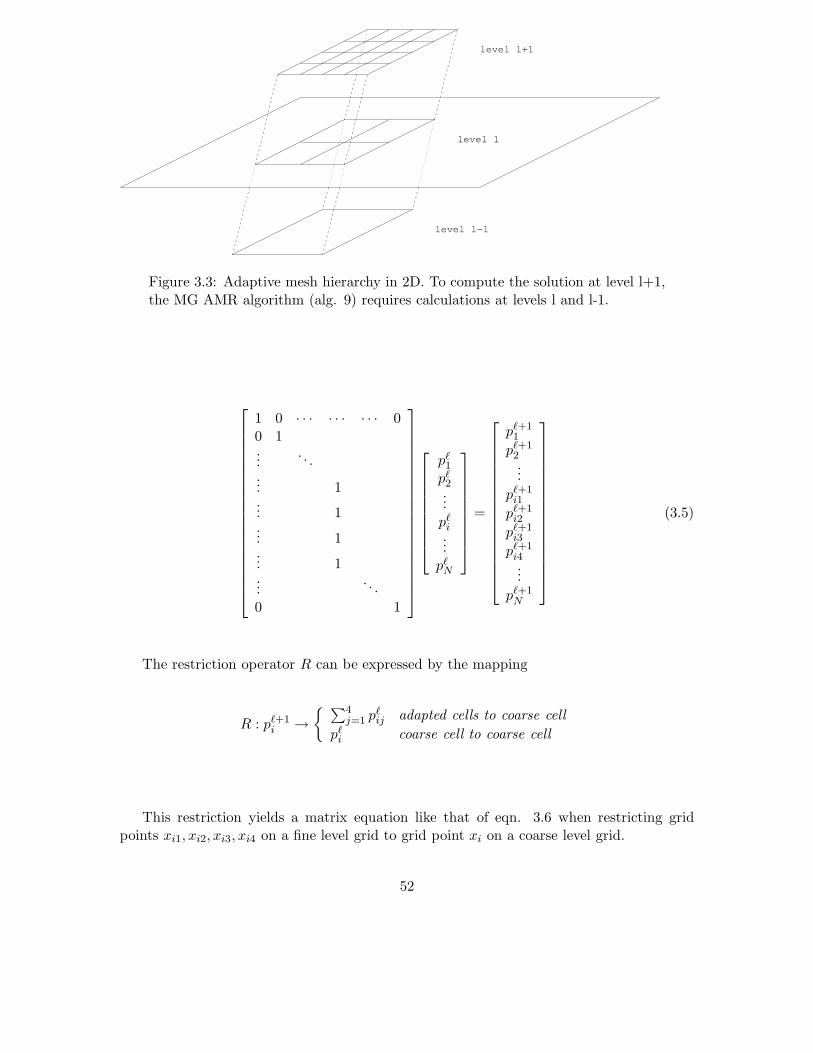
level l+1

level l

level l−1

Figure 3.3: Adaptive mesh hierarchy in 2D. To compute the solution at level l+1,the MG AMR algorithm (alg. 9) requires calculations at levels l and l-1.

1 0 · · · · · · · · · 00 1...

. . .... 1... 1... 1... 1...

. . .

0 1

pℓ1

pℓ2...pℓ

i...

pℓN

=

pℓ+11

pℓ+12...

pℓ+1i1

pℓ+1i2

pℓ+1i3

pℓ+1i4...

pℓ+1N

(3.5)

The restriction operator R can be expressed by the mapping

R : pℓ+1i →

{ ∑4j=1 pℓ

ij adapted cells to coarse cell

pℓi coarse cell to coarse cell

This restriction yields a matrix equation like that of eqn. 3.6 when restricting gridpoints xi1, xi2, xi3, xi4 on a fine level grid to grid point xi on a coarse level grid.

52

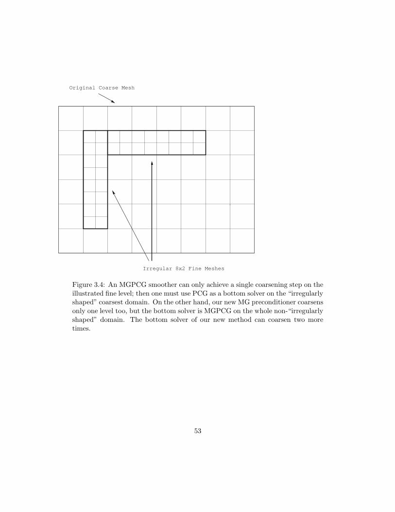
Irregular 8x2 Fine Meshes

Original Coarse Mesh

Figure 3.4: An MGPCG smoother can only achieve a single coarsening step on theillustrated fine level; then one must use PCG as a bottom solver on the “irregularlyshaped” coarsest domain. On the other hand, our new MG preconditioner coarsensonly one level too, but the bottom solver is MGPCG on the whole non-“irregularlyshaped” domain. The bottom solver of our new method can coarsen two moretimes.

53

1 0 · · · · · · · · · · · · · · · · · · 00 1...

. . .... 1 1 1 1...

. . .

0 1

pℓ+11

pℓ+12...

pℓ+1i1

pℓ+1i2

pℓ+1i3

pℓ+1i4...

pℓ+1N

=

pℓ1

pℓ2...pℓ

i...

pℓN

(3.6)

Matrix eqns. 3.5 and 3.6 show that the restriction and prolongation operators are trans-poses of each other.

In order to show that algorithm 10 converges, it is sufficient to show that it meetsthe criteria set forth by Tatebe [76] for convergence of the MGPCG method, i.e. 1) theMG smoother is symmetric, 2) the restriction operator is the transpose of the prolongationoperator, and 3) the matrix A in the smoothing step

xk+1 = xk + M(b − Axk) real cells

xk+1 = xk fictitious cells

is symmetric. One can see that condition 2 is satisfied by viewing the matrix operatorsfor the restriction and prolongation, and A will be symmetric as long as first order bound-ary conditions are applied [53, 54], so it is sufficient to show that the MG preconditionerproduced by relaxAMR is symmetric. To show that the MG preconditioner on an adaptivegrid is symmetric, we will assume that the grid on each level is a union of ‘real’ fine cellsand ‘fictitious’ coarse cells such as depicted in figure 3.5. Let M be a symmetric precon-ditioner produced by ILU on a uniform grid, then we will define the corresponding AMRpreconditioner on a given level ℓ by the matrix M , which can be defined as

M =

{

M real cells0 fictitious cells

and our equivalent smoothing step is simply xk+1 = xk + M(b −Axk). Now, if one were toorder the cells in such a manner that the variables corresponding to real cells were listedfirst, e.g.

[x1, x2, · · · , xN ] → [xreal1 , xreal

2 , · · · , xrealn , xfictitious

1 , xfictitious2 , · · · , xfictitious

n ]

then we find that

54

Real Cell Fictitious Cell

Figure 3.5: Coarse and fine grid levels depicting real and fictitious cells.

M =

[

M 00 0

]

which is symmetric and so algorithm 10 is guaranteed to converge.

3.2.4 2D Bubble

The first problem we will discuss is that of a 3D axisymmetric gas bubble (2 com-putational dimensions) rising through a liquid phase. Figure 3.6 displays representativediscretization grids for this problem with increasing numbers of adaptive levels. Timingdata for this problem is given in table 3.3 and a table giving the speedup factor of the newMGPCG AMR algorithm over the original MG AMR algorithm is provided in table 3.4. Onthis problem, the new MGPCG AMR algorithm is typically 2-3X faster than the originalMG AMR algorithm, and performs up to 4X faster than the original MG AMR algorithmwhen using a blocking factor of four along with five adaptive levels. The only case whenthe new solver underperforms is with a blocking factor of eight and only one adaptive level.

3.2.5 3D Bubble

The second test problem is also a rising gas bubble through a liquid phase, but expandedto three spatial dimensions. Figure 3.7 shows the grid for this problem with two adaptivelevels and a blocking factor of four. Timing data for this problem is given in table 3.5 and atable giving the speedup factor of the new MGPCG AMR algorithm over the original MGAMR algorithm is provided in table 3.6. For this test problem, the new MGPCG AMRalgorithm shows improvement over the MG AMR algorithm when more than one adaptive

55

a. b.

c. d.

Figure 3.6: AMR grids for a rising 3D axisymmetric bubble. The representativegrids all use a blocking factor of two and contain a) one adaptive level, b) twoadaptive levels, c) three adaptive levels, and d) four adaptive levels.

56

Table 3.3: Timing results for a single pressure solve for the new MGPCG AMRalgorithm along with the old MG AMR algorithm and the PCG algorithm for the3D axisymmetric test bubble. The new MGPCG algorithm is faster than the oldMG AMR algorithm in nearly every scenario. Grid sizes for a fixed blocking factorand number of adaptive levels are identical for each method.

Blocking Factor 2 4 8Adaptive Levels 1 3 5 1 3 5 1 3 5

ILU SmootherPCG 0.659 5.424 63.49 0.563 3.359 35.54 0.365 2.875 26.78MG 0.270 2.181 13.93 0.252 1.349 10.05 0.098 0.751 6.060MGPCG 0.142 0.636 4.109 0.127 0.439 2.493 0.096 0.382 2.156

ICRB SmootherPCG 0.653 5.366 69.49 0.567 3.561 39.02 0.377 3.012 25.53MG 0.281 2.177 16.54 0.278 1.435 10.96 0.112 0.885 6.634MGPCG 0.157 0.655 4.511 0.152 0.498 2.732 0.123 0.415 2.402

GSRB SmootherPCG 0.641 5.706 65.99 0.567 4.037 37.72 0.364 3.014 29.26MG 0.284 2.165 13.91 0.266 1.367 10.38 0.108 0.845 5.957MGPCG 0.153 0.678 4.426 0.145 0.464 2.743 0.118 0.408 2.176

Table 3.4: Speedup factor for the new MGPCG AMR method over the original MGAMR method on the 3D axisymmetric test bubble problem. The new algorithmoutperforms the old by an increasing margin as both the blocking factor and thenumber of adaptive levels are increased. It can be seen that the benefits of the newmethod are not realized in the case of large blocking factors and a single adaptivelevel.


ILU 1.91X 3.43X 3.39X 1.99X 3.07X 4.03X 1.01X 1.97X 2.81XICRB 1.79X 3.32X 3.67X 1.83X 2.88X 4.01X 0.91X 2.13X 2.76XGSRB 1.86X 3.19X 3.14X 1.84X 2.95X 3.78X 0.92X 2.07X 2.74X

57

Y

Z

X

Figure 3.7: Mesh for a 3D rising bubble with 2 adaptive levels and a blocking factor of 4.

level is used and achieves a speedup of 2X in the case of three adaptive levels and a blockingfactor of two.

3.2.6 3D Whale

The third problem tested here is simulated flow past a 3D whale body. Figure 3.8 showsa grid with two adaptive levels for this problem, along with the whale body. This testproblem shows the best overall speedup of the new method and is 2-4X faster than the oldmethod, even when only solving with one adaptive level.

3.3 FUN3D

The software accelerated in this section is the NASA FUN3D code, which is describedin references [5] and [4]. Additionally, the acceleration found here was first described in

58

Table 3.5: Timing results for a single pressure solve for the new MGPCG AMRalgorithm along with the old MG AMR algorithm and the PCG algorithm for a3D test bubble.



ICRB SmootherPCG 4.158 19.67 75.61 3.682 15.28 56.82 4.770 27.19 84.94MG 2.227 9.916 41.31 1.910 6.958 30.35 2.490 10.10 28.47MGPCG 2.354 7.083 19.36 2.263 5.950 16.96 2.686 7.559 20.33

GSRB SmootherPCG 4.023 19.99 78.66 3.735 15.43 58.33 4.801 26.19 86.51MG 2.145 9.708 41.06 1.860 7.086 31.98 2.485 10.10 29.68MGPCG 2.331 7.149 20.20 2.241 6.191 17.67 2.571 8.001 20.19

Table 3.6: Speedup factor for the new MGPCG AMR method over the original MGAMR method on the 3D test problem of simulating a gas bubble rising through aliquid phase.



59

X

Z

Y

Figure 3.8: Mesh for a 3D whale with 2 adaptive levels.

60

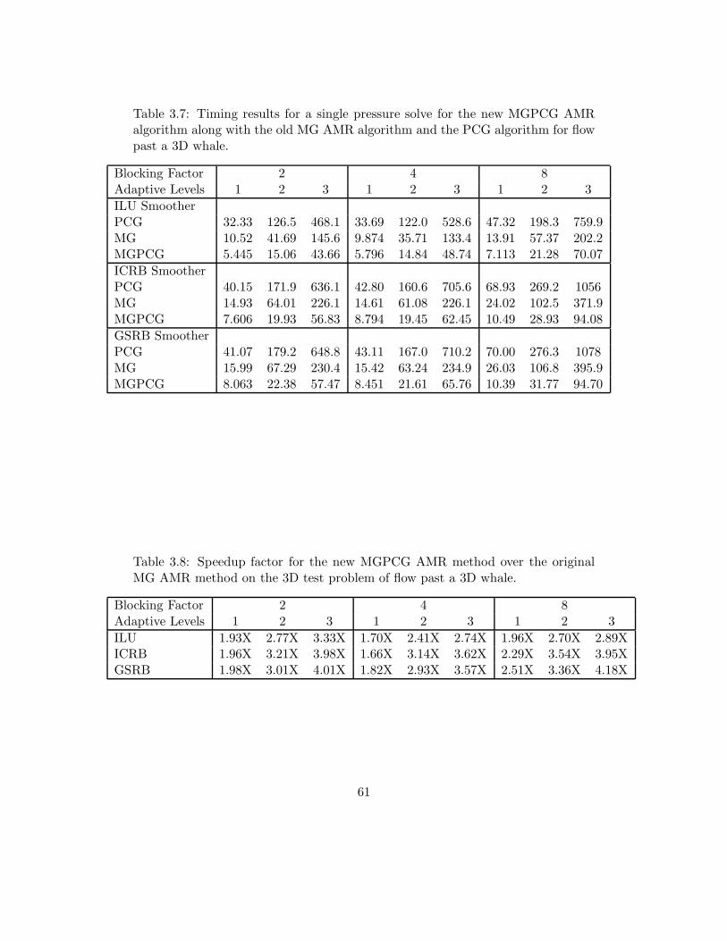
Table 3.7: Timing results for a single pressure solve for the new MGPCG AMRalgorithm along with the old MG AMR algorithm and the PCG algorithm for flowpast a 3D whale.



ICRB SmootherPCG 40.15 171.9 636.1 42.80 160.6 705.6 68.93 269.2 1056MG 14.93 64.01 226.1 14.61 61.08 226.1 24.02 102.5 371.9MGPCG 7.606 19.93 56.83 8.794 19.45 62.45 10.49 28.93 94.08

GSRB SmootherPCG 41.07 179.2 648.8 43.11 167.0 710.2 70.00 276.3 1078MG 15.99 67.29 230.4 15.42 63.24 234.9 26.03 106.8 395.9MGPCG 8.063 22.38 57.47 8.451 21.61 65.76 10.39 31.77 94.70

Table 3.8: Speedup factor for the new MGPCG AMR method over the originalMG AMR method on the 3D test problem of flow past a 3D whale.



61

[21]. FUN3D is a large production level code consisting of several hundred Fortran 95modules and approximately 850,000 lines of code. Under development since the late 1980’s,FUN3D possesses a large array of aerodynamic simulation and optimization capabilities forboth steady and time dependent problems across the speed range. The software has beendistributed to hundreds of individuals in academia, industry and other goverment agencies.This work focuses on the porting of a single routine (point implicit colored GS solver) whichconsumes a substantial portion of the computation.

3.3.1 Mathematical Formulation

The portion of the FUN3D code pertinent to this work is the compressible Reynolds-averaged Navier-Stokes solver. The spatial discretization utilizes an unstructured finitevolume scheme with a tetrahedral mesh. The dependent variables are stored at the vertices.Inviscid fluxes at control volume interfaces are computed using the upwind scheme of Roe[67], and viscous fluxes are formed using an approach equivalent to a finite-element Galerkinprocedure [5]. For turbulent flows, the eddy viscosity is modeled using the one-equationapproach of Spalart and Allmaras [69]. An approximate solution of the linear system ofequations formed within each time step is obtained through several iterations of a multicolorpoint-iterative scheme. The turbulence model is integrated all the way to the wall withoutthe use of wall functions and is solved separately from the mean flow equations at each timestep with a time integration and linear system solution scheme identical to that employedfor the mean flow equations. In the current implementation, the grid points are numberedusing a reverse Cuthill- McKee technique [16] to improve cache performance during flux andjacobian gather/scatter operations. However, the multicolor point-iterative scheme forbidsphysically adjacent unknowns from residing within the same color group. Therefore, therelaxation scheme is inherently cache unfriendly in its basic form. Since the majority of thefloating point operations required to advance the solution take place in the relaxation phase,a mapping is introduced which orders the data in the coefficient matrix by its assigned coloras the individual contributions to the jacobian elements are determined. In this manner,memory is accessed in ideal sequential order during the relaxation as would be achieved ina more simplistic scheme such as point-Jacobi, while the substantial algorithmic benefits(improved stability and convergence) of the multicolor scheme are retained.

3.3.2 Parallelization and Scaling

The FUN3D code has demonstrated parallel scalability to tens of thousands of proces-sor cores. This is achieved primarily through efficiient domain decomposition and messagepassing communication. Pre- and post-processing operations are also performed in parallelusing distributed memory, avoiding the need for a single image of the mesh or solution atany time and ultimately yielding a highly efficient end- to-end simulation paradigm. Typi-cal scaling performance for the solver on a range of mesh sizes is shown in Figure 3.9, withmeshes in the millions of nodes. A mesh typically contains six times as many tetrahedralcells than the number of nodes, and so the 105 million node mesh equates to 630 milliontetrahedral cells. The majority of these results have been generated on a Silicon Graph-ics ICE platform consisting of dual-socket, quad-core Intel Xeon “Harpertown” processors.The data marked “Westmere” has been generated using dual- socket, hex-core “Westmere”

62

102

103

104

102

103

CPU Cores

FU

N3D

CP

U T

ime

(S)

Ares 52M NodesLinear (Ideal)DPW4 105M Nodes (Westmere)DPW4 35M NodesDPW2 12M NodesDPW2 65M Nodes DPW4 105M Nodes

Figure 3.9: Parallel scaling results for FUN3D. Problems are given by node size,with M equating to millions of nodes. There are approximately 6 times as manytetrahedral cells as there are nodes for a given problem size. Ares is a rocket geom-etry and DPW grids represent aircraft configurations from AIAA Drag PredictionWorkshops. The linear dashed line represents ideal scaling.

processors. The implementation scales well across the range of processing cores shown.

One factor in maintaining scalable performance within FUN3D is the load balancing ofthe computation and communication costs over the processors, which inherently involves theefficient partitioning of the underlying unstructured grid. The mesh partitioning softwareMetis and ParMetis [47, 48] is used by many CFD codes. Metis’ partitioning objectivesattempt to evenly distribute the number of nodes (work) to each processor, while minimizingthe number of adjacent elements assigned to different processors (communication). In graphtheory, these objectives translate to minimizing the edge-cuts and minimizing the totalcommunication volume.

3.3.3 GPU Acceleration

To improve the performance of the FUN3D code, a minimally invasive accelerator modelhas been implemented in which code portions are ported to the GPU. This allows for an

63

increase in speed without altering the proven methods of the underlying solvers. TheFUN3D code portion targeted for acceleration was the point implicit subroutine used forgroups of 5x5 matrix equations which represent the linearized form of the discrete meanflow equations. These correspond to the density, velocity and pressure variables ρ, u, v,w, and p. This routine can account for as much as 70% of the program’s total CPUtime (such as when solving the Euler equations), but is typically closer to 30% (RANS),depending on the required number of sweeps by the colored Gauss-Seidel (GS) solver for theparticular problem. Cache size can play a significant role on this routine and on unstructuredcodes in general. For this reason along with the need for concurrent kernel executioncapabilities, only the latest generation Nvidia Fermi architecture hardware is targeted, sincethese possesses true L1 and L2 caches which were previously unavailable. On the CPU side,each core performs the colored GS solve sequentially, so a natural mapping to the GPU iscreated with single threads computing the solutions to the individual 5x5 block solves ofa color in parallel. A CUDA C subroutine call has been inserted into the original Fortranpoint_solve_5 (PS5) subroutine to carry out the code porting. The computation of theright hand side (RHS) solve between colors has effectively been moved to the GPU whensufficient available memory and double precision capabilities are present. A general outlineof PS5 is given in Algorithm 1, noting single precision (SP), double precision (DP) andmixed precision (MP) segments. For the test problems, 10,000’s to 100,000’s of threads arelaunched, each computing an entire 5x5 block solve corresponding to an individual equationfor the particular color. CUDA C was chosen because it allows for the most explicit usercontrol over the previously mentioned Fermi architecture GPUs that we are employing asaccelerators. CUDA C also provides portability as it is is widely used and the compiler isfreely available. Given the code, one could (with a little effort) extend this capability toother accelerators with OpenCL, as the language extensions are similar. In general, anyaccelerator used must have capabilities for both concurrent kernel execution and doubleprecision arithmetic, though there are exceptions that will be discussed further.

Algorithm 11 PS5 Subroutine Outline

for color = 1 to max colors do

b(:) = residual(:)// Begin RHS solvefor n = start to end do

Step 1. Compute off diagonal contributionsfor j = istart to iend do

bi = bi − Σi6=jAi,j ∗ xicol (SP)end for

Step 2. Compute 5x5 forward solve (DP)Step 3. Compute 5x5 back solve (DP)Step 4. Compute sum contribution, update RHS (MP)Step 5. Accumulate Sum Contributions (GPU Only)

end for

// End color, do MPI communicationCall MPI transfer

end for

64

3.3.4 GPU Distributed Sharing Model

The GPU code has been developed with four different CUDA subroutines; the firstdedicated for a single core-single GPU scenario, and the remaining three for multi-corescenarios which require MPI communication transfers at the end of each color sweep. TheMPI versions are based on what we call a GPU distributed sharing model. We will definethis as an accelerator model where work is efficiently distributed across multiple processorswhich share a single GPU. This should be done in such a manner that, if necessary, theCPU cores perform some amount of the computational work which would otherwise be doneby the GPU in order to ensure that kernel execution remains optimal. This is an impor-tant concept since large kernels can place large demands on available GPU resources whencalled simultaneously, particularly when they use many registers and large chunks of sharedand constant memory. In fact, if too many resources are required, kernels from multiplethreads could be scheduled to execute sequentially, causing a substantial or complete lossof performance gains. Sharing kernel work with multiple CPU threads should also reducecore idle time, leading to more resource efficient execution. One constraint we have foundinherent to this model is a reduction in available GPU memory. As data is distributed tomultiple CPU cores, there are more individual structures that are padded when put intoGPU memory, leading to a reduction in the available global memory for each additionalthread. In all of our test cases on a GTX 480 card, each additional thread sharing the GPUreduces the available global memory predictably within the 63-68 MB range, independentof problem size. This yields an average loss of approximately 66.7 MB of available memoryper shared CPU thread, for exactly the same amount of data being stored.

We consider GPU sharing to be an important feature of new and future hybrid CFDcodes. We recognize that on a large shared hybrid cluster one could simply use one coreper GPU, allowing the remaining cores of a node to be allocated to other tasks. However,with a scalable CFD code it is optimal to utilize as many cores as possible, since this shouldlead to the best overall performance. Consider running a CFD code that easily scales tothousands of cores on a 256 GPU cluster. Clearly, one would produce better times with1024 cores and 256 GPUs than with only 256 cores and 256 GPUs, even if the speedup overthe CPU cores alone was not as dramatic.

We will now present the four new CUDA subroutines introduced into the FUN3D code,and note that only solution data transfers to and from the GPU are required within thesubroutine itself. All other necessary data is transferred externally in optimal locations.Also note that these subroutines only replace a single sweep of the colored GS solver, asMPI communications are typically necessary after every sweep.

3.3.5 CUDA Subroutines

• gs_gpu : The first subroutine is for a straightforward 1 core - 1 GPU setup where theentire GS solve is done in CUDA. The kernel for this scenario computes the entire RHSsolve, and is called repeatedly through the color sweeps without any data transfers. Inthis case, a single GPU thread maps to a single control volume, computing its own 5x5

65

block solve (steps one through four in Algorithm 1). After a thread synchronization,the kernel keeps five threads to accumulate the sum contributions for the five variables(step 5 of Algorithm 1) before moving on to the next color. This scenario does notrequire MPI communication, and hence provides the biggest performance gains, but islimited to a single processor. We will refer to this routine as gs_gpu, which does notrequire concurrent kernel execution. The kernel for this routine allocates 21 registersper thread, and 136 bytes of constant memory per thread block at compile time,as found by the --ptxas-options=-v compiler option. It requires one CPU to GPUsolution transfer at the beginning of the call, and one GPU to CPU transfer at the end,but none between colors. We note that our unstructured code is unable to effectivelyuse the 48 KB shared memory space, and opt instead to swap this larger section withthe 16 KB L1 cache space using the cudaFuncSetCacheConfig function. Using thelarger L1 cache space provides a noticeable 6% performance increase over the smallerversion for this routine.

• gs_mpi0 : This case is identical to that above in terms of the GPU kernel, however,it assumes that an MPI communication is required at the end of each color. Here,the CUDA routine must copy the solution back from the GPU and return it to theFortran subroutine to perform the transfer, providing additional overhead. We willrefer to this routine as gs_mpi0, which uses the same kernel as gs_gpu and hencemaintains identical GPU resource allocation properties. This routine, along with theother MPI CUDA routines, require two additional data transfers (one CPU to GPUand one GPU to CPU) for each color.

• gs_mpi1 : This subroutine is the first to consider the effects of GPU sharing, byattempting to reduce the kernel size and distribute a small portion of the workloadto the CPU. When developing kernels, one must try to reduce CPU-GPU memorycopies at all costs, even if that means performing less than ideal tasks on the GPUside. The kernel of the first two subroutines performs a final accumulation of sumcontributions with a mere 5 threads, and so this portion of code does not benefitfrom mass thread parallelism, but does reduce transfer overhead by keeping sumcontributions on the GPU. As more threads share the GPU, this potential overheadcan be reduced since multiple CPU cores can copy their respective sum contributionsback in parallel. Once there, the more powerful CPU cores should be able to performthe accumulations faster. This concept is implemented in subroutine gs_mpi1. Movingthis small amount of work to the CPU reduces the constant memory by a mere 8 bytesand does not reduce the kernel register count.

• gs_mpi2 : The final subroutine was designed to execute with many threads sharing asingle GPU. It shares a substantial amount of computation with the CPU, and alsoeliminates all double precision calculations from the GPU side. This is accomplishedby cutting the kernel short and computing the double precision forward and backwardsolves along with the sum and solution updates on the CPU, only computing step 1of Algorithm 1 on the GPU. In the process, the need to transfer the diagonal of theLHS matrix A is eliminated, leading to a reduction in data transfer costs and moreimportantly, freeing up valuable global memory space. The kernel for this subrou-

66

Table 3.9: FUN3D Grid partitioning over 8 processor cores, showing that nodedistributions are fairly well balanced.

Cores 1 2 3 4 5 6 7 8

1 3392062 168161 1710454 85339 84626 84861 843808 42824 40608 42828 42622 42555 42525 42726 42518

tine reduces the register count by 1, while maintaining the same constant memoryrequirements as the kernel of gs_mpi1.

3.4 Test Problems

The GPU accelerated FUN3D code has been tested with a number of problem sizesranging from approximately 16,000 to 1.1 million grid points (96,000 - 6.6 million elements),but will describe in more detail two particular scenarios.

3.4.1 Test Problem 1

The first test problem is a generic wing-body geometry used in grid generation trainingat NASA Langley [3]. It is a pure tetrahedral grid, with 37,834 triangular boundary faces,339,206 Nodes and 1,995,247 Cells. The node partitioning is given in Table 3.9, the surfacegrid is given in Figure 3.10, along with the GPU computed pressure solution for p

p∞at

convergence. This setup calls 20 PS5 sweeps per iteration, accounting for approximately70% of the FUN3D total run time. This problem is inviscid, has a Mach number of 0.3 andan angle of attack of 2.0 degrees.

3.4.2 Test Problem 2

The second problem is a DLR-F6 wing-body configuration used in the second interna-tional AIAA Drag Prediction Workshop (DPW-II) [51]. The versions used here include thecoarse grid containing 1,121,301 nodes and 6,558,758 tetrahedral cells, and also a reducedgrid with approximately 650,000 nodes and 3.9 million tetrahedral cells. In this case, PS5corresponds to approximately 30% of the total FUN3D wall clock time. The smaller gridalong with the corresponding GPU computed pressure solution for p

p∞are given in Fig-

ure 3.11, corresponding to a turbulent solution with a Mach number of 0.76, an angle ofattack of 0.0 degrees and a Reynolds number of 1 million.

3.5 FUN3D Results and Discussion

Two machines were used for timing studies: a dual socket Dell workstation with IntelXeon 5080 CPUs (2 cores @ 3.73 GHz, 2 MB L2) and a single Nvidia GTX 480 GPU. Thesecond machine is a small Beowulf GPU cluster with a head node and two Fermi equipped

67

0.9 0.92 0.94 0.96 0.98 1 1.02 1.04 1.06 1.08 1.1 1.12

Figure 3.10: Test problem 1 grid (left) and GPU computed pressure solution forp

p∞(right). Generic wing-body geometry, contains 339,206 nodes and 1,995,247

tetrahedral cells. Pressure solution obtained at convergence of the FUN3D solver(132 iterations). Inviscid, Mach Number = 0.3, Angle of Attack = 2.0 degrees.

0.9 0.92 0.94 0.96 0.98 1 1.02 1.04 1.06 1.08

Figure 3.11: Test problem 2 grid (left) and GPU computed pressure solution forp

p∞(right). DLR-F6 wing-body configuration, contains approximately 650,000

nodes and 3.9 million tetrahedral cells. Turbulent, Mach Number = 0.76, Angleof Attack = 0.0 degrees, Reynolds Number = 1, 000, 000.

68

Table 3.10: Single core performance results for routine gs gpu on test problem 1using the GTX 480 WS.

GTX 480 WS - gs_gpu CPU Cores CPU Time CPU/GPU Time Speedup

FUN3D Code 1 1732.8 s 794.1 s 2.182XPS5 Subroutine 1 0.455 s 0.082 s 5.549X

compute nodes connected by a gigabit switch. Each compute node possesses an AMDAthlon II X4 620 processor (4 cores @ 2.6 GHz, 2 MB L2) and a single Nvidia GTX 470card. We note that we have recently gained access to a GPU research cluster at Nvidiacorporation and have begun further testing on a much larger scale, with acces to 96 CPUcores and 16 Tesla Fermi GPUs. We do not include any conclussions from this furtherstudy here as it is not yet complete, but note that some initial timing data is included inAppendix A, along with more detailed data using the machines mentioned here.

3.5.1 Single Core Performance

Performance results for a single sweep of the PS5 solver on the GTX 480 workstationfor a range of grid point sizes are given in Figure 3.12. The best performing subroutine,gs_gpu, achieves a speedup of approximately 5.5X regardless of problem size. Performancefor the gs_mpi0 routine which utilizes the same CUDA kernel is cut in half as a resultof CPU-GPU data transfers necessary for MPI communication between colors. We seethat version gs_mpi2 comes closest to the performance of gs_gpu, and believe that thisis due to the removal of double precision calculations, as the GeForce series cards havebeen purposely de-tuned for these. We speculate that gs_mpi1 would achieve the bestMPI performance in the presence of higher end Tesla series cards with full double precisioncapabilities. Single core speedups on the Beowulf cluster are not as good, with a best caseof 4.75X. This is due to the fact that the CPU times are slightly better on a single AMDcore, and that the GTX 470 is slightly less capable than the 480 model. For the singlecore scenario on both machines, the overall FUN3D code is accelerated by a factor of 2Xor more for test problem 1, which spends about 70% of its total CPU time in the PS5subroutine. We note that our CUDA subroutines execute the fastest with only 8-16 threadsper block, well below the Nvidia minimum recommendation of 64. This is likely due tothe additional cache resources available to each thread. While we are primarily concernedwith large scale parallel applications, these single core results provide valuable insight. Wehave learned here that even in the absence of MPI transfers, speedups are limited and wellbelow the par set by so many other GPU acclerated applications. We do note, however,that larger cache sizes could help narrow the gap between this unstructured code and thosethat benefit from ordered memory access patterns. We also find that in a single core settingour GPU accelerated implicit solver has exceeded the 2.5-3X speedup achieved by that ofthe OVERFLOW code [46], perhaps a more fitting standard for comparison.

69

Table 3.11: Single core performance results for routine gs gpu on test problem 1using the GTX 470 BC.

GTX 470 BC - gs_gpu CPU Cores CPU Time CPU/GPU Time Speedup


400 500 600 700 800 9000

0.2

0.4

0.6

0.8

1

1.2

1.4

Grid Points (Thousands)

PS

5 T

ime

(s)

CPUgs_gpugs_mpi0gs_mpi1gs_mpi2

Figure 3.12: CPU and GPU performances for a single PS5 sweep with varying testcase sizes. Tests were run on a single core of an Intel Xeon 5080 CPU mated witha single NVIDIA GTX 480 GPU.

70

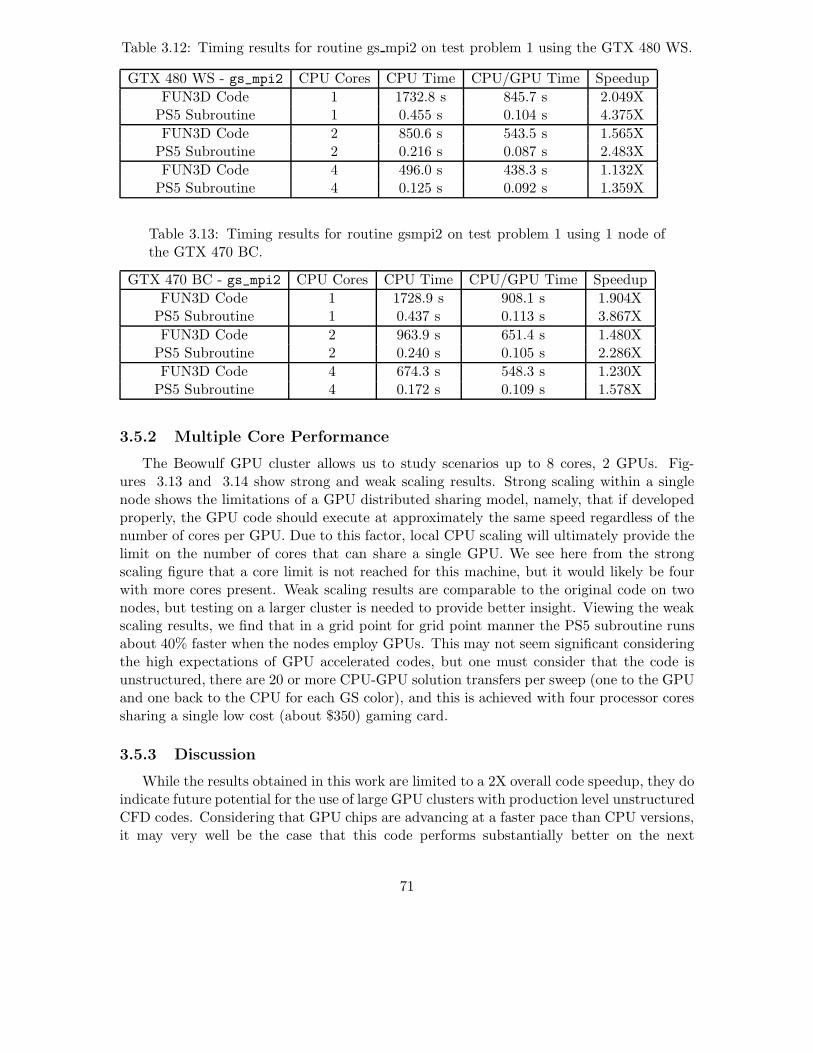
Table 3.12: Timing results for routine gs mpi2 on test problem 1 using the GTX 480 WS.

GTX 480 WS - gs_mpi2 CPU Cores CPU Time CPU/GPU Time Speedup




Table 3.13: Timing results for routine gsmpi2 on test problem 1 using 1 node ofthe GTX 470 BC.

GTX 470 BC - gs_mpi2 CPU Cores CPU Time CPU/GPU Time Speedup




3.5.2 Multiple Core Performance

The Beowulf GPU cluster allows us to study scenarios up to 8 cores, 2 GPUs. Fig-ures 3.13 and 3.14 show strong and weak scaling results. Strong scaling within a singlenode shows the limitations of a GPU distributed sharing model, namely, that if developedproperly, the GPU code should execute at approximately the same speed regardless of thenumber of cores per GPU. Due to this factor, local CPU scaling will ultimately provide thelimit on the number of cores that can share a single GPU. We see here from the strongscaling figure that a core limit is not reached for this machine, but it would likely be fourwith more cores present. Weak scaling results are comparable to the original code on twonodes, but testing on a larger cluster is needed to provide better insight. Viewing the weakscaling results, we find that in a grid point for grid point manner the PS5 subroutine runsabout 40% faster when the nodes employ GPUs. This may not seem significant consideringthe high expectations of GPU accelerated codes, but one must consider that the code isunstructured, there are 20 or more CPU-GPU solution transfers per sweep (one to the GPUand one back to the CPU for each GS color), and this is achieved with four processor coressharing a single low cost (about $350) gaming card.

3.5.3 Discussion

While the results obtained in this work are limited to a 2X overall code speedup, they doindicate future potential for the use of large GPU clusters with production level unstructuredCFD codes. Considering that GPU chips are advancing at a faster pace than CPU versions,it may very well be the case that this code performs substantially better on the next

71

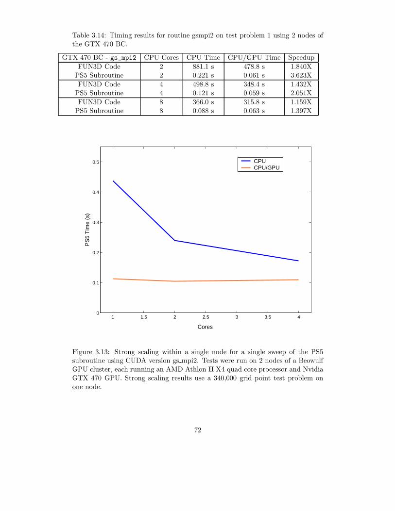
Table 3.14: Timing results for routine gsmpi2 on test problem 1 using 2 nodes ofthe GTX 470 BC.





1 1.5 2 2.5 3 3.5 40

0.1

0.2

0.3

0.4

0.5

Cores

PS

5 T

ime

(s)

CPUCPU/GPU

Figure 3.13: Strong scaling within a single node for a single sweep of the PS5subroutine using CUDA version gs mpi2. Tests were run on 2 nodes of a BeowulfGPU cluster, each running an AMD Athlon II X4 quad core processor and NvidiaGTX 470 GPU. Strong scaling results use a 340,000 grid point test problem onone node.

72

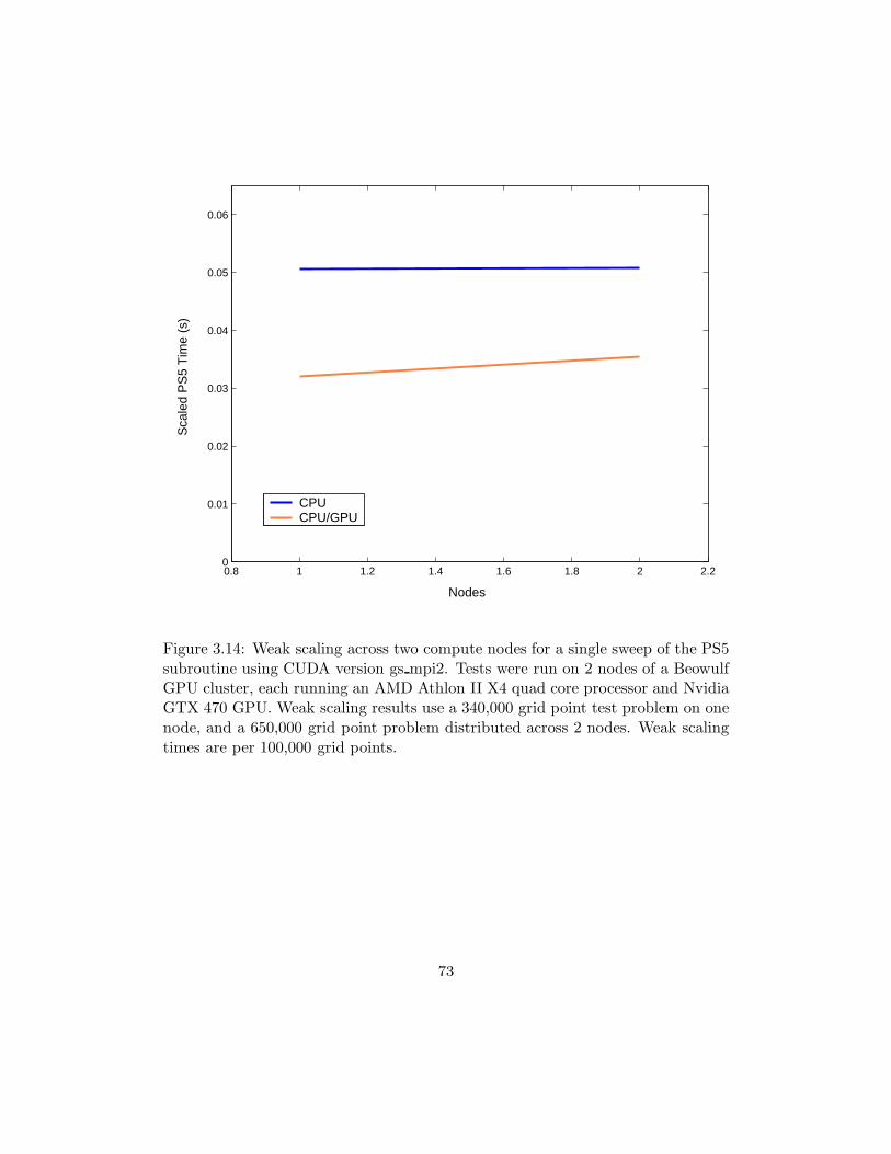
0.8 1 1.2 1.4 1.6 1.8 2 2.20

0.01

0.02

0.03

0.04

0.05

0.06

Nodes

Sca

led

PS

5 T

ime

(s)

CPUCPU/GPU

Figure 3.14: Weak scaling across two compute nodes for a single sweep of the PS5subroutine using CUDA version gs mpi2. Tests were run on 2 nodes of a BeowulfGPU cluster, each running an AMD Athlon II X4 quad core processor and NvidiaGTX 470 GPU. Weak scaling results use a 340,000 grid point test problem on onenode, and a 650,000 grid point problem distributed across 2 nodes. Weak scalingtimes are per 100,000 grid points.

73

Table 3.15: GPU architecture evolution from G80, which approximately coincidedwith the release of Intel’s quad core CPUs, to Fermi which coincided with therelease of Intel’s six core processors. GPU advancements over the last few yearshave noticeably outpaced those of CPUs. Representative GPUs are: G80-GeForce8800 GT, GT200-Tesla C1060, Fermi-Tesla C2050. 1shared memory, 2 texturememory, 3Configurable L1/shared memory.

Architecture Year Cores L1 Cache L2 Cache Memory Access Speed

G80 2006 112 16 KB 1 128 KB 2 57.6 GB/s GDDR3GT200 2008 240 24 KB 1 256 KB 2 102 GB/s GDDR3Fermi 2010 448 48/16 KB 3 768 KB 144 GB/s GDDR5

generation architecture with larger cache sizes and faster memory access speeds. Table 3.15provides a look at the rapid advancements occurring in GPU technology, which is beginningto noticeably outpace those of CPUs. Should these trends continue with more availablecache and faster memory access speeds, hybrid clusters will become much more amenableto the acceleration of unstructured codes. However, if GPUs are to play an integral role inlarge scale parallel computations invovling high level codes, data transfer technologies willalso need to improve to reduce the performance penalty incurred through CPU-GPU datatransfers, as these will provide the biggest bottleneck.

74

CHAPTER 4

FUTURE RESEARCH

In this chapter we bring together the work on PDE constrained optimization and on CFDcode acceleration and look forward to the the development of a simulation based designcode for microfluidic applications. While significant contributions to this dissertation comefrom the study of adjoint methods and the acceleration of the FUN3D code, we note thatgradient based aerodynamic design via adjoint methods is well studied and that this isone of FUN3D’s current capabilities. The acceleration of the FUN3D point implicit solvershould directly provide accelerated adjoint based design capabilities (adjoint solvers essen-tially require two flow solves per iteration), but we will not pursue this topic any furtherhere. We also note that we are currently working in the early stages of a collaborationwith Nvidia Corporation and the Computational AeroSciences Branch at NASA LangleyResearch Center to further develop FUN3D on GPU based clusters. Since the future direc-tion of this work is uncertain at this time, we can not include any specific discussion here.In addition, we are also developing an improved version of the GPU accelerated CLSVOFprojection smoothers which will use CUDA instead of the PGI Fortran Accelerator. We willnow move on to discuss the development of a code for the numerical design of microfluidicT-junctions used in lab-on-a-chip devices.

4.1 Towards the Computational Design of Microfluidic

Structures

An SBD application we are interested in is the design of midrofluidic T-junctions forlab-on-a-chip designs. This work is a planned collaboration with Micheal Roper’s (FSUChemistry) microfluids lab who will provide experimental data for verification of our nu-merical models. The main idea of the so called ‘Lab on a Chip’ setup is to allow for varioushigh throughput assay applications in which the reactions of precisely measured dropletsare observed in microfluidic channels. Recent research and applications of such devices aredescribed in the works [27,68,75], which also provide a solid foundation of information relat-ing to the aspect of droplet break up in T-junction geometries. In order to create dropletsof a particular size, microfluidic T-junctions are employed; see the left side of Figure 4.1.We can see from the figure that the junction consists of two channels, a horizontal channelwhich contains a continuous or ’carrier’ fluid, and another channel perpendicularto to thefirst channel which contains the discontinuous fluid which forms the droplets. In [27], a good

75

discussion of droplet and bubble formation and breakup in both liquid-liquid and gas liquidsystems is given along with associated findings on the relationships between various inputfactors such as fluid pressures and viscosities for particular setups. It is in this work that wefind two important conditions in the ’squeezing’ mechanism which leads to droplet rupture,first that the width of the main channel should be greater than its height, and second thatthe width of the inlet channel be at least half the main channel’s width. While this workprovides some guidance for the design of T-junctions under certain conditions, the modelsfound through experimentation break down once parameters are changed. We feel that thisis a problem which can be best tackled by simulation based design utilizing state of the artalgorithms for both simulating the fluid flow through these microfluidic channels, and foroptimizing the design of the T-junction itself. From Figure 4.1 (left side) one can see thatthe basic design of a T-junction can be described using the precise height and width of theindividual channels. We propose to use varying control points within the T-junction whichcan be shifted to produce simulations resulting in droplets of varying sizes. The precisionin the size of these drops is important as they travel through the trap array since they maynot be properly caught if they are not the correct size.. Other important factors whichcontribute to the control of the droplets include the surfactants used in the process andthe flow rates of the individual phases (e.g. oil and water), variables which can easily beincorporated into a non-intrusive derivative free optimization strategy.

Numerical simulations of the T-junction geometries using data from Roper’s lab setupare given in figure 4.2. We propose to use our CLSVOF code along with a MGMDSalgorithm to carry out the design optimization of the channel dimension, first using only asmall number of control points to define the geometry. As the project progresses we intendto include more design variables including surfactant properties. The end result will be astate-of-the-art microfluidic design code capable of producing optimal channel designs fortwo phase flows at the micro level.

76

Figure 4.1: Microfluidic T-junction experiment from Roper’s laboratory (FSUChemistry) showing a T-junction geometry with a droplet traveling via a carrierfluid.

Figure 4.2: Numerical simulations of two fluids in a microfluidic T-junction usingthe CLSVOF code and experimental setups from Roper’s Lab.

77

CHAPTER 5

CONCLUSION

In this dissertation we have provided valuable knowledge to the fields of PDE constrainedoptimization, multigrid methods, incompressible multiphase flow simulations on adaptivemeshes and GPU computing methods for CFD codes. Furthermore, we have provided aframework with which to move forward towards the the development of a sophisticateddesign code for microfluidic structures. To this end we have provided the following specificadvances to applied and computational mathematics:

• We have demonstrated that the gradient free multidirectional search method (MDS)is a viable alternative to the discrete adjoint method for problems in PDE constrainedoptimization when one only requires a local method, and when gradient computationis not feasible. We estimate that in the case that there are as many processor coresavailable for computation as the number of design variables plus one (each processorcore maps in parallel to a PDE solve) that the MDS method will perform on par withthe discrete adjoint method run on a single processor core. In addition, we have foundthat the MDS method is not as sensitive to non-linear model features as is the discreteadjoint method for the 1D data assimilation problems tested.

• We have shown that multigrid schemes can significantly accelerate the convergencerate of the multidirectional search method when employed in the solution of PDEconstrained optimization methods. Using an FMG cycle, we have demonstrated a5.5X speedup on a linear 1D data assimilation problem. We have also shown forthis problem that the use of weighted averaging of the fine grid solution through themultigrid cycles can produce a more accurate final solution, but at the cost of fastersolution times.

• We have described the GPU acceleration of the smoothing steps required by a pre-conditioned conjugate gradient solver used in the solution of the pressure projectionstep of a coupled level set and volume of fluid code (CLSVOF). This GPU acceleratedsolver utilizes PGI Fortran compiler with accelerator directives. We have shown thatfor a large aspect ratio 2D problem, the new accelerated solver is up to 2.4X fasterthan the CPU version. We have concluded that a new solver should be developedin the compute unified device architecture (CUDA) language which allows for moredirect user control over data allocation, and which will allow us to permanently store

78

data on the GPU. This should substantially reduce communication overhead betweenthe GPU and CPU and lead to a much faster code.

• We have described an improved pressure projection solver for incombressible multi-phase flow simulations on adaptive grids which requires substantially fewer grid pointcalculations than current methods. The new MGPCG AMR method is up to 4X fasterthan the previous MG AMR algorithm for the problems tested.

• We have ported the point_solve_5 subroutine of the unstructured NASA FUN3Dcode for computation on GPU based clusters, achieving a speedup of up to 5.5X forthe subroutine and up to 2X for the overall code. The new subroutine utilizes anovel GPU sharing model that allows multiple processor cores to run on a single GPUsimultaneously, and provides for increased scalability. We have shown that this modelscales in parallel up to 8 cores - 2 GPUs, and that a 40% performance increase for theaccelerated subroutine has been achieved with 4 cores sharing a single GPU.

79

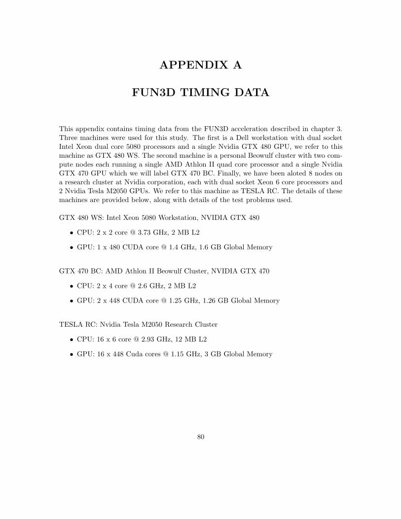
APPENDIX A

FUN3D TIMING DATA

This appendix contains timing data from the FUN3D acceleration described in chapter 3.Three machines were used for this study. The first is a Dell workstation with dual socketIntel Xeon dual core 5080 processors and a single Nvidia GTX 480 GPU, we refer to thismachine as GTX 480 WS. The second machine is a personal Beowulf cluster with two com-pute nodes each running a single AMD Athlon II quad core processor and a single NvidiaGTX 470 GPU which we will label GTX 470 BC. Finally, we have been aloted 8 nodes ona research cluster at Nvidia corporation, each with dual socket Xeon 6 core processors and2 Nvidia Tesla M2050 GPUs. We refer to this machine as TESLA RC. The details of thesemachines are provided below, along with details of the test problems used.

GTX 480 WS: Intel Xeon 5080 Workstation, NVIDIA GTX 480

• CPU: 2 x 2 core @ 3.73 GHz, 2 MB L2

• GPU: 1 x 480 CUDA core @ 1.4 GHz, 1.6 GB Global Memory

GTX 470 BC: AMD Athlon II Beowulf Cluster, NVIDIA GTX 470

• CPU: 2 x 4 core @ 2.6 GHz, 2 MB L2

• GPU: 2 x 448 CUDA core @ 1.25 GHz, 1.26 GB Global Memory

TESLA RC: Nvidia Tesla M2050 Research Cluster

• CPU: 16 x 6 core @ 2.93 GHz, 12 MB L2

• GPU: 16 x 448 Cuda cores @ 1.15 GHz, 3 GB Global Memory

80

Table A.1: Test problems used in this study. * approximate.

Problem Configuration Type Cells Nodes

Test Problem 1 Simple Wing/Body Inviscid 339,206 1,995,247Test Problem 2 DLR-F6 Aircraft Turbulent 650,000* 3,900,000*Test Problem 3 Wing Leading-Edge Turbulent 900,000* 5,500,000*Test Problem 4 DLR-F6 Aircraft - Turbulent 1,121,301 6,558,758

Table A.2: Timing results for routine gs gpu on test problem 1 using the TESLA RC.

TESLA RC - gs_gpu CPU Cores CPU Time CPU/GPU Time Speedup

PS5 Subroutine 1 0.17497 s 0.096 s 1.822X

Table A.3: Timing results for routine gs mpi0 on test problem 1 using the GTX 480 WS.





Table A.4: Timing results for routine gs mpi0 on test problem 1 using 1 node ofthe GTX 470 BC.





Table A.5: Timing results for routine gs mpi0 on test problem 1 using 2 nodes ofthe GTX 470 BC.





81

Table A.6: Timing results for routine gs mpi1 on test problem 1 using the GTX 480 WS.





Table A.7: Timing results for routine gs mpi1 on test problem 1 using 1 node ofthe GTX 470 BC.





Table A.8: Timing results for routine gs mpi1 on test problem 1 using 2 nodes ofthe GTX 470 BC.





Table A.9: Timing results for routine gs mpi2 on test problem 1 using 1 node ofthe TESLA RC.




Table A.10: Timing results for routine gs gpu on test problem 2 using the GTX 480 WS.

GTX 480 WS gs_mpi2 CPU Cores CPU Time CPU/GPU Time Speedup


82

Table A.11: Timing results for routine gs gpu on test problem 2 using the GTX 470 BC.



Table A.12: Timing results for routine gs mpi2 on test problem 2 using the GTX480 WS.





Table A.13: Timing results for routine gs mpi2 on test problem 2 using two nodesof the GTX 470 BC machine.










Table A.15: Timing results for routine gs mpi2 on test problem 3 using the GTX480 WS machine.




Table A.16: Timing results for routine gs mpi2 on test problem 3 using two nodesof the GTX 470 BC machine. GPU Memory is insufficient for sharing among 4threads, the problem must be split across two GPUs.





83





Table A.18: Timing results for routine gs mpi2 on test problem 4 using eight nodesof the TESLA RC machine.

TESLA RC - gs_mpi2 CPU Cores CPU Time CPU/GPU Time Speedup


84

BIBLIOGRAPHY

[1] www.top500.org, last accessed Aug. 5, 2010.

[2] http://www.green500.org, last accessed Aug. 16th, 2010.

[3] http://tetruss.larc.nasa.gov, last accessed Aug. 13, 2010.

[4] http://fun3d.larc.nasa.gov, last accessed Jan. 2, 2011.

[5] W.K. Anderson and D.L. Bonhaus. An implicit upwind algorithm for computing tur-bulent flows on unstructured grids. Comput. Fluids, 23(1):1–21, 1994.

[6] D. Aurox and J. Blum. Data assimilation methods for an oceanographic problem.volume Lecture Notes XVI of Mathematics in Industry. Springer-Verlag, 2004.

[7] M. J. Berger and P. Colella. Local adaptive mesh refinement for shock hydrodynamics.J. Comp. Phys., 82:64–84, 1989.

[8] M. J. Berger and J. Oliger. Adaptive mesh refinement for hyperbolic partial differentialequations. J. Comp. Phys., 53:484–512, 1984.

[9] J. Brezillon and N.R. Gauger. 2D and 3D aerodynamic shape optimisation using theadjoint approach. Aerospace Science and Technology, 8:715–727, 2004.

[10] W. L. Briggs, V. E. Henson, and S. F. McCormick. A Multigrid Tutorial. SIAM,Philadelphia, PA, USA, second edition, 2000.

[11] E. F. Campana, D. Peria, Y. Tahara, and F. Stern. Shape optimization in ship hy-drodynamics using computational fluid dynamics. Comput. Meth. Appl. Mech. Eng.,196(3):634–651, 2006.

[12] G. Carpenteiri, B. Koren, and M.J.L. van Tooren. Adjoint-based shape optimizationon unstructured meshes. Journal of Computational Physics, 224:267–287, 2007.

[13] J. M. Cohen and M. J. Molemaker. A fast double precision CFD code using cuda. InProceedings of Parallel CFD 2009, 2009.

[14] NVIDIA Corporation. NVIDIA CUDA Programming Guide, version 2.2, April 2009.

[15] A. Corrigan, F. Camelli, R. Lohner, and J. Wallin. Running unstructured grid basedCFD solvers on modern graphics hardware. In 19th AIAA CFD Conference, SanAntonio, Texas, USA, June 2009.

85

[16] E. Cuthill and J. McKee. Reducing the bandwidth of sparse symmetric matrices. InProceedings of the 24th Nat. Conf. ACM, pages 157–172, 1969.

[17] J.E. Dennis and V. Torczon. Direct search methods on parallel machines. SIAMJournal of Optimization, 1(4):448–474, 1991.

[18] D. Dommermuth, M. Sussman, R. Beck, T. O’Shea, and D. Wyatt. The numerical sim-ulation of ship waves using cartesian grid methods with adaptive mesh refinement. InProccedings of the Twenty Fifth Symposium on Naval Hydr., St. Johns, New Foundlandand Labrador, Canada, 2004.

[19] J. Dongarra, I. Foster, G. Fox, W. Gropp, K. Kennedy, L. Torczon, and A. White,editors. The Sourcebook of Parallel Computing. The Morgan Kaufmann Series inComputer Architecture and Design. Elsevier, November 2002.

[20] D. Drikakis, O. P. Iliev, and D. P. Vassileva. A nonlinear multigrid method for the threedimensional incompressible Navier-Stokes equations. J. Comput. Phys., 146(1):301–321, 1998.

[21] A. C. Duffy, D. P. Hammond, and E. J. Nielsen. Production level CFD code accelera-tion for hybrid many-core architechtures. Parallel Comput., 2011. Accepted, pendingrevisions.

[22] E. Elsen, P. LeGresley, and E. Darve. Large calculation of the flow over a hypersonicvehicle using a GPU. J. Comput. Phys., 227:10148–10161, 2008.

[23] J. Dongarra et. al. Exascale roadmap 1.0, 2010.

[24] F. Fang, C.C. Pain, M.D. Piggott, G.J. Gorman, and A.J.H Goddard. An adaptivemesh adjoint data assimilation method applied to free surface flows. Int. J. Numer.Methods Fluids, 47:995–1001, 2005.

[25] F. Fang, M.D. Piggott, C.C. Pain, G.J. Gorman, and A.J.H Goddard. An adaptivemesh adjoint data assimilation method. Ocean Model., 15:39–55, 2006.

[26] D. Furbish, M.Y. Hussaini, F.-X. Le Dimet, and P. Ngnepieba. On discretization errorand its control in varational data assimilation. Tellus A, 60:979–991, 2008.

[27] P. Garstecki, M. Fuerstman, H. Stone, and G. Whitesides. Formation of droplets andbubbles in a microfluidic t-junction–scaling and mechanism of break-up. Lab Chip,6:437–446.

[28] D. Goddeke, S. H. Buijssen, H. Wobker, and S. Turek. GPU acceleration of an unmod-ified parallel finite element navier-stokes solver. In High Performance Computing andSimulation 2009, Leipzig, Germany, June 2009.

[29] D. Goddeke and R. Strzodka. Cyclic reduction tridiagonal solvers on GPUs applied tomixed precision multigrid. IEEE T. Parall. Distr., March 2010. Special Issue: HighPerformance Computing with Accelerators.

86

[30] D. Goddeke, R. Strzodka, J. Mohd-Yusof, P. McCormick, S. H. Buijssen, M. Grajewski,and S. Turek. Exploring weak scalability for FEM calculations on a GPU enhancedcluster. Parallel Comput., 33(10-11):685–699, 2007.

[31] D. Goddeke, R. Strzodka, J. Mohd-Yusof, P. McCormick, H. Wobker, C. Becker, andS. Turek. Using GPUs to improve multigrid solver performance on a cluster. Int. J.Comput. Sci. Eng., 4(1):36–55, 2008.

[32] M. Griebel and P. Zaspel. A multi-gpu accelerated solver for the three-dimensionaltwo-phase incompressible navier-stokes equations. Comput Sci Res Dev, 25:65–73,April 2010.

[33] A. K. Griffith and N.K. Nichols. Data assimilation using optimal control theory. Nu-merical analysis report, The University of Reading, October 1994.

[34] B. E. Griffith, R. D. Hornung, D. M. McQueen, and C. S. Peskin. An adaptive, formallysecond order accurate version of the immersed boundary method. J. Comput. Phys.,223:10–49, 2007.

[35] Y. Ha and S. Cho. Shape sensitivity analysis for incompressible fluid using SPH pro-jection method. In 8th. World Congress on Computational Mechanics, 5th. EuropeanCongress on Computational Methods in Applied Sciences and Engineering, Venice,Italy, June 2008.

[36] J. P. Hamalainen, R. E. Makinen, and P. Tarvainen. Evolutionary shape optimizationin CFD with industrial applications. In European Congress on Computational Methodsin Science and Engineering, 2000.

[37] J. Haslinger and R.A.E. Makinen. Introduction to Shape Optimization: Theory, Ap-prximation and Computation. Advances in Design and Control. SIAM, Philadelphia,PA, USA, 2003.

[38] P. W. Hemker, B. Koren, and S. P. Spekreijse. A nonlinear multigrid method for theefficient solution of the steady Euler equations. Lect. Notes Phys., 264:308–313, 1986.

[39] R. M. Hicks, E. M. Murman, and G. N. Vanderplaats. An assessment of airfoil design bynumerical optimization. Technical Report TM X-3092, NASA, Ames Research Center,Moffett Field, CA, USA, July 1974.

[40] D. Isebe, P. Azerad, F. Bouchette, B. Ivorra, and B. Mohammadi. Shape optimizationof geotextile tubes for sandy beach protection. Int. J. Numer. Methods Eng., 2007.

[41] D. Isebe, P. Azerad, B. Mohammadi, and F. Bouchette. Optimal shape design ofdefense structures for minimizing short wave impact. Coastal Eng., 55:35–46, 2008.

[42] D.A. Jacobsen, J. Thibault, and I. Senocak. An MPI-CUDA implementation for mas-sively parallel incompressible flow computations on multi-GPU clusters. In 48th AIAAAerospace Sciences Meeting, Orlando, Florida, USA, January 2010.

87

[43] D.A. Jacobsen, J.C. Thibault, and I. Senocak. An MPI-CUDA implementation formassively parallel incompressible flow computations on Multi-GPU clusters. In 48thAIAA Aerospace Sciences Meeting, Orlando, FL U.S.A., January 2010.

[44] A. Jameson and L. Martinelli. A continuous adjoint method for unstructured grids. InAIAA Paper 03-3955, 16th AIAA CFD Conference, pages 23–26, 2003.

[45] A. Jameson, S. Shakaran, and L. Martinelli. Continuous adjoint method for unstruc-tured grids. AIAA J., 46(5):1226–1239, 2008.

[46] D. C. Jesperson. Acceleration of a cfd code with a gpu. NAS Technical Report NAS-09-003, NASA Ames Research Center, November 2009.

[47] G. Karypis and V. Kumar. Multilevel algorithms for multi-constraint graph partition-ing. In Proceedings of the 1998 ACM/IEEE SC98 Conference, 1998.

[48] G. Karypis and V. Kumar. Multilevel k-way partitioning scheme for irregular graphs.J. Parallel Distrib. Comput., 48(1):96–129, 1998.

[49] V. Kindratenko, J. Enos, G. Shi, M. Showerman, G. Arnold, J. Stone, J. Phillips, andW. Hwu. GPU clusters for high-performance computing. In IEEE Cluster 2009, NewOrleans, Louisiana, USA, Aug. - Sept. 2009.

[50] E. Laporte and P. Le Tallec. Numerical Methods in Sensitivity Analysis and ShapeOptimization. Modeling and Simulation in Science, Engineering and Technology.Birkhauser, 2003.

[51] E.M. Lee-Rausch, N.T. Frink, D.J. Mavriplis, R.D. Rausch, and W.E. Milholen. Tran-sonic drag prediction on a DLR-F6 transport configuration using unstructured gridsolvers. Comput. Fluids, 38:511–532, 2009.

[52] R. M. Lewis and S. G. Nash. Model problems for the multigrid optimization of systemsgoverned by differential equations. SIAM J. Sci. Comp., 26(6):1811–1837, 2005.

[53] F. Losasso, R. Fedkiw, and S. Osher. Spatially adaptive techniques for level set methodsand incompressible flow. Comput. Fluids, 35(10):995–1010, 2006.

[54] F. Lossaso, F. Gibou, and R. Fedkiw. Simulating water and smoke with an octree datastructure. ACM Trans. Graph., 23:457–462, 2004.

[55] C. A. Mader, J. R. R. A. Martins, J. J. Alonso, and E. Van Der Weide. ADjoint: Anapproach for the rapid developement of discrete adjoint solvers. AIAA J., 46(4):863–873, 2008.

[56] A. McNamara, A. Treuille, Z. Popovic, and J. Stam. Fluid control using the adjointmethod. ACM Trans. Graphics, 23:449–446, 2004.

[57] S. K. Nadarajah and A. Jameson. Optimum shape design for unsteady three-dimensional viscous flows using a non-linear frequency domain method. In AIAA paper2006-3455, 24th Applied Aerodynamics Conference, San Francisco, CA, USA, 2006.

88

[58] S. G. Nash. A multigrid approach to discretized optimization problems. Optim. Meth.Softw., 14:99–116, 2000.

[59] M. Nemec and M. J. Aftsomis. Adjoint formulation for an embedded-boundary carte-sian method. In AIAA paper 2005-4987, 17th Computational Fluid Dynamics Confer-ence, Toronto, ON, CAN, 2005.

[60] M. Nemec, M. J. Aftsomis, S. M. Murman, and T. H. Pulliam. Adjoint formulation foran embedded-boundary cartesian method. In 43rd AIAA Aerospace Sciences Meeting,Reno, NV, USA, 2005.

[61] R. Nourgaliev, S. Kadioglu, and V. Mousseau. Marker redistancing/level set methodfor high-fidelity implicit interface tracking. SIAM J. Sci. Comput., 32(1):320–348, 2010.

[62] J. M. Ortega. Introduction to Parallel and Vector Solution of Linear Systems. Frontiersof Computer Science. Plenum Press, New York, NY, 1988.

[63] E. H. Phillips, Y. Zhang, R. L. Davis, and J. D. Owens. Rapid aerodynamic perfor-mance prediction on a cluster of graphics processing units. In Proceedings of the 47thAIAA Aerospace Sciences Meeting, Orlando, Florida, USA, January 2009.

[64] S. A. Ragab. Shape optimization in free surface potential flow using an adjoint formu-lation. Hydrodynamics Directorate Technical Report NSWCCD-50-TR-2003/33, NavalSurface Warfare Center, Carderock Division, West Bethesda, MD, USA, August 2003.

[65] S. A. Ragab. Shape optimization of surface ships in potential flow using an adjointformulation. AIAA J., 42(2):296–304, 2004.

[66] A. R. Robinson and P. F.J. Lermusiaux. Overview of data assimilation. HarvardReports in Physical/Interdisciplinary Ocean Science 62, Harvard University, 2000.

[67] P.L. Roe. Approximate riemann solvers, parameter vectors, and difference schemes. J.Comp. Phys., 43(2):357–372, 1981.

[68] W. Shi, J. Qin, N. Ye, and B. Lin. Droplet-based microfluidic system for individualCaenorhabditis elegans assay. Lab Chip, 8:1432–1435, 2008.

[69] P.R. Spalart and S.R. Allmaras. A one-equation turbulence model for aerodynamicflows. Rech. Aerospatiale, 1:5–21, 1994.

[70] P. Stewart, N. Lay, M. Sussman, and M. Ohta. An improved sharp interface methodfor viscoelastic and viscous two-phase flows. J. Sci. Comput., 35(1):43–61, 2008.

[71] M. Sussman. A parallelized, adaptive algorithm for multiphase flow in general geome-tries. Comput. Struct., 83:435–444, 2005.

[72] M. Sussman, A. Almgren, J. Bell, P. Colella, L. Howell, and M. Welcome. An adaptivelevel set approach for incompressible two-phase flows. J. Comput. Phys., 148:81–124,1999.

89

[73] M. Sussman, K. Smith, M. Hussaini, M. Ohta, and R. Zhi-Wei. A sharp interfacemethod for incompressible two-phase flows. J. Comput. Phys., 221(2):469–505, 2007.

[74] Y. Tahara, F. Stern, and Y. Himeno. Computational fluid dynamics-based optimizationof a surface combatant. J. Ship Res., 48(4):273–287, 2004.

[75] W.-H. Tan and S. Takeuchi. A trap-and-release integrated microfluidic system fordynamic microarray applications. PNAS, 104(4):1146–1151, 2007.

[76] O. Tatebe. The multigrid preconditioned conjugate gradient method. In 6th CopperMountain Conference on Multigrid Methods, Copper Mountain, CO, USA, April 1993.

[77] J. C. Thibault and I. Senocak. Cuda implementation of a Navier-Stokes solver on multi-GPU desktop platforms for incompressible flows. In 47th AIAA Aerospace SciencesMeeting, Orlando, Florida, USA, January 2009.

[78] V. Torczon. Multi-Directional Search: A Direct Search Algorithm for Parallel Ma-chines. PhD thesis, Rice University, May 1989.

[79] V. Torczon. On the convergence of the multidirectional search algorithm. SIAM J.Optim., 1(1):123–145, 1991.

[80] B. G. van Bloemen Waanders, R. A. Bartlett, S. S. Collis, E. R. Keiter, C. C. Ober,T. M. Smith, V. Akcelik, O. Ghattas, J. C. Hill, M. Berggren, M. Heinkenschloss, andL. C. Wilcox. Sensitivity technologies for large scale simulation. Technical ReportSAND2004-6574, Sandia National Laboratories, January 2005.

[81] J. Waltz and R. Lohner. A grid coarsening algorithm for unstructured multigrid appli-cations. In 38th AIAA Aerospace Sciences Meeting and Exhibit, AIAA-00-0925, Reno,NV, USA, 2000.

[82] Q. Wang, D. Gleich, A. Saberi, N. Etemadi, and P. Moin. A Monte Carlo method forsolving unsteady adjoint equations. J. Comput. Phys., 227:6184–6205, 2008.

90

BIOGRAPHICAL SKETCH

Austen Duffy was born in East Stroudsburg, Pennsylvania on August 16, 1980 to parentsFrancis J. and Bonnie L. Duffy. He grew up in the Pocono Mountains region of northeast-ern Pennsylvania, graduating from Pocono Mountain Senior High School in 1999. In 2003,Austen recieved his B.S. in Mathematics from York College of Pennsylvania, a small pri-vate liberal arts school in southcentral Pennsylvania. Upon recieving his bachelors degree,Austen began his graduate education at Indiana University of Pennsylvania, and recieved aterminal M.S. in Applied Mathematics in 2005 before entering the Ph.D. program in Appliedand Computational Mathematics at Florida State University. Austen’s research interestsare primarily computational in nature, with an emphasis towards real world applicationsin science and engineering. In addition to his time as a teaching and research assistant,Austen has worked as a visiting researcher at the National Institute of Aerospace and theNASA Langley Research Center.

91

the florida state university massively … · the florida state university college of arts and...

Documents