the fors deep field: field selection, photometric ... filee-mail: [email protected] based...

A&A 398, 49–61 (2003)DOI: 10.1051/0004-6361:20021620c© ESO 2003

Astronomy&

Astrophysics

The FORS Deep Field: Field selection, photometric observationsand photometric catalog�,��

J. Heidt1, I. Appenzeller1, A. Gabasch2, K. Jager3, S. Seitz2, R. Bender2, A. Bohm3, J. Snigula2, K. J. Fricke3,U. Hopp2, M. Kummel4, C. Mollenhoff1, T. Szeifert5, B. Ziegler3,6, N. Drory2, D. Mehlert1, A. Moorwood7,

H. Nicklas3, S. Noll1, R. P. Saglia2, W. Seifert1, O. Stahl1, E. Sutorius1,8, and S. J. Wagner1

1 Landessternwarte Heidelberg, Konigstuhl, 69117 Heidelberg, Germany2 Universitatssternwarte Munchen, Scheinerstr. 1, 81679 Munchen, Germany3 Universitats-Sternwarte Gottingen, Geismarlandstr. 11, 37083 Gottingen, Germany4 Max-Planck-Institut fur Astronomie, Konigstuhl 17, 69117 Heidelberg, Germany5 European Southern Observatory Santiago, Alonso de Cordova 3107, Santiago 19, Chile6 Akademie der Wissenschaften, Theaterstr. 7, 37079 Gottingen, Germany7 European Southern Observatory, Karl-Schwarzschild-Str. 2, 85748 Garching, Germany8 Royal Observatory Edinburgh, Blackford Hill, Edinburgh EH9 3HJ, UK

Received 11 July 2002 / Accepted 15 October 2002

Abstract. The FORS Deep Field project is a multi-colour, multi-object spectroscopic investigation of a ∼7′ × 7′ region nearthe south galactic pole based mostly on observations carried out with the FORS instruments attached to the VLT telescopes. Itincludes the QSO Q 0103-260 (z = 3.36). The goal of this study is to improve our understanding of the formation and evolutionof galaxies in the young Universe. In this paper the field selection, the photometric observations, and the data reduction aredescribed. The source detection and photometry of objects in the FORS Deep Field is discussed in detail. A combined B and Iselected UBgRIJKs photometric catalog of 8753 objects in the FDF is presented and its properties are briefly discussed. Theformal 50% completeness limits for point sources, derived from the co-added images, are 25.64, 27.69, 26.86, 26.68, 26.37,23.60 and 21.57 in U, B, g, R, I, J and Ks (Vega-system), respectively. A comparison of the number counts in the FORS DeepField to those derived in other deep field surveys shows very good agreement.

Key words. methods: data analysis – catalogs – galaxies: general – galaxies: fundamental parameters – galaxies: photometry

1. Introduction

Deep field studies have become one of the most powerful toolsto explore galaxy evolution over a wide redshift range. One ofthe main aims of this kind of study is to constrain current evolu-tionary scenarios for galaxies, such as the hierarchical structureformation typical of Cold Dark Matter universes.

Undoubtedly, the Hubble Deep Field North (HDF-N,Williams et al. 1996) and follow-up observations with Keckwere of particular importance to improve our knowledge of

Send offprint requests to: J. Heidt,e-mail: [email protected]� Based on observations collected with the VLT−UT1 on Cerro

Paranal (Chile) and the NTT on La Silla (Chile) operated by theEuropean Southern Observatory in the course of the observing pro-posals 63.O-0005, 64.O-0149, 64.O-0158, 64.O-0229, 64.P-0150 and65.O-0048.�� The full version of Table 4 is only available in electronicform at the CDS via anonymous ftp to cdsarc.u-strasbg.fr(130.79.128.5) or viahttp://cdsweb.u-strasbg.fr/cgi-bin/qcat?J/A+A/398/49

galaxy evolution in the redshift range z = 1−4 (see e.g. thecontributions to the HDF symposium, 1998, ed. Livio et al.).The HDF-N is the deepest multi-colour view of the sky madeso far, with excellent resolution. A disadvantage of the HDF-N (and its southern counterpart, the Hubble Deep Field South(HDF-S, Williams et al. 2000)) is a relatively small field ofview (∼5.6 sq.arcmin). Therefore, its statistical results may beaffected by the large-scale structure (Kajisawa & Yamada 2001;see also Cohen 1998) and by limitations due to small samples.

Following the pioneering work of Tyson (1988) severalground-based deep fields with a wide range of scientific drivers,sizes, limiting magnitudes and resolutions have been initiated.Examples are the NTT SUSI Deep Field (NTTDF, Arnoutset al. 1996), which has a size similar to the HDFs and sub-arcsecond resolution, but is a few magnitudes less deep than theHDFs, or the William Herschel Deep Field (WHTDF, Metcalfeet al. 2001 and references therein), which has a much largerfield of view, a depth comparable to the HDFs, but lacks sub-arcsecond resolution. Other surveys, such as the Calar AltoDeep Imaging Survey (CADIS, Meisenheimer et al. 1998), are

50 J. Heidt et al.: The FORS Deep Field

Fig. 1. DSS plots of the FDF and of a field of the same size surrounding the HDF-S. Also indicated are the field boundaries of the HDF-S. Notethe much lower surface density of bright foreground objects and the absence of bright stars in the FDF region.

much shallower, but cover much larger areas (several 100 sq.arcmin in the case of CADIS ) and are specifically designed tosearch for primeval galaxies in the redshift range z = 4.6−6.7.

The aim of the FORS Deep Field (FDF) is to merge someof the strengths of the deep field studies cited above. The FDFprogramme has been carried out with the ESO VLT and theFORS instruments (Appenzeller et al. 1998) at a site, that of-fers excellent seeing conditions and allows imaging to almostthe depths of the HDFs. The larger field of view compared tothe HDFs (about 4 times the combined HDFs) alleviates theproblem of the large-scale structure and results in larger sam-ples of interesting objects. Moreover, spectroscopic follow-upstudies with FORS can make full use of the entire field. Usingthe FORS2 MXU-facility, up to ∼60 spectra of galaxies (within40 slitlets) in the FDF can be taken simultaneously.

In the present paper, the field selection of the FDF, the pho-tometric observations and the data reduction are described. Thefirst results have been described in Jager et al. (1999). A sourcecatalog (available electronically) based on objects detected inthe B and I bands and containing 8753 objects in the FDF isdescribed and its properties are discussed. This catalog super-sedes a preliminary I-band selected catalog, which had beendiscussed by Heidt et al. (2000). Photometric redshifts obtainedfrom the FDF will be discussed by Gabasch et al. (in prep.;see Bender et al. 2001 for preliminary results). Spectroscopicfollow-up observations of a subsample of the FDF galaxieshave been started. Up to now, spectra of about 500 galaxieswith redshifts up to z ∼ 5 have been analyzed. Initial resultshave been described in Appenzeller et al. (2002), Mehlert et al.(2001, 2002), Noll et al. (2001) and Ziegler et al. (2002).

2. Field selection

A critical aspect for a deep field study is the selection of a suit-able sky area. Since we intended to obtain a representative deepcosmological probe of the Universe, one condition was that thegalaxy number counts were not disturbed by a galaxy clusterin the field. To go as deep as possible also requires low galac-tic extinction (E(B − V) < 0.02 mag). For the same reason,the field had to be devoid of strong radio or X-ray sources (po-tentially indicating the presence of galaxy clusters at medium

Table 1. Characteristics of the FORS Deep Field.

Field center 1h6m3.s6 − 25◦45′46′′ (2000)mean E(B − V) 0.018H I column density 1.92 × 1020 cm−2

Radio sources (NVSS) none with flux > 2.5 mJyIRASCirrus (100 µm) 0.035 JyBright stars (<5 mag) none within 5◦

redshifts). On the other hand, we decided to include a high-redshift (z > 3) radio-quiet QSO to study the IGM along theline-of-sight to the QSO and the QSO environment. To facili-tate the observations in other wavebands, low HI column den-sity (<2×1020 cm−2) and low FIR cirrus emission was required.Moreover, stars brighter than 18th mag had to be absent to al-low reasonably long exposures, to avoid saturation of the CCDand to minimize readout time losses. Because of the latter con-ditions, the HDF-S region was not suitable for our study (seeFig. 1). Additionally, stars brighter than 5th mag within 5◦ ofthe field had to be absent to avoid possible reflexes and stray-light from the telescope structure. Finally, the field had to havea good observability and, therefore, had to pass close to thezenith at the VLT site.

Due to these constraints, the south galactic pole regionwas searched for a suitable field. We started by selecting allthe QSOs from the catalog of Veron-Cetty & Veron (7th edi-tion, 1997) with z > 3 within 10◦ of the south galactic pole.This resulted in 32 possible field candidates. Next we didan extensive search in the literature from radio up to the X-ray regime (FIRST, IRAS maps, RASS etc.), checked visu-ally the digitized sky survey and used the photometry providedby the COSMOS scans to select 4 promising field candidatescontaining a z > 3 QSO. For these 4 field candidates shorttest observations were carried out during the commissioningphase of FORS1, which showed that 3 of them were not useful(they either contained conspicuous galaxy clusters or, in onecase, did not provide suitable guide stars for the active op-tics of the VLT). Finally, a field with the center coordinatesα2000 = 1h6m3.s6, δ2000 = −25◦45′46′′ containing the QSO Q0103-260 (z = 3.36, Warren et al. 1991) was chosen as the FDF.

J. Heidt et al.: The FORS Deep Field 51

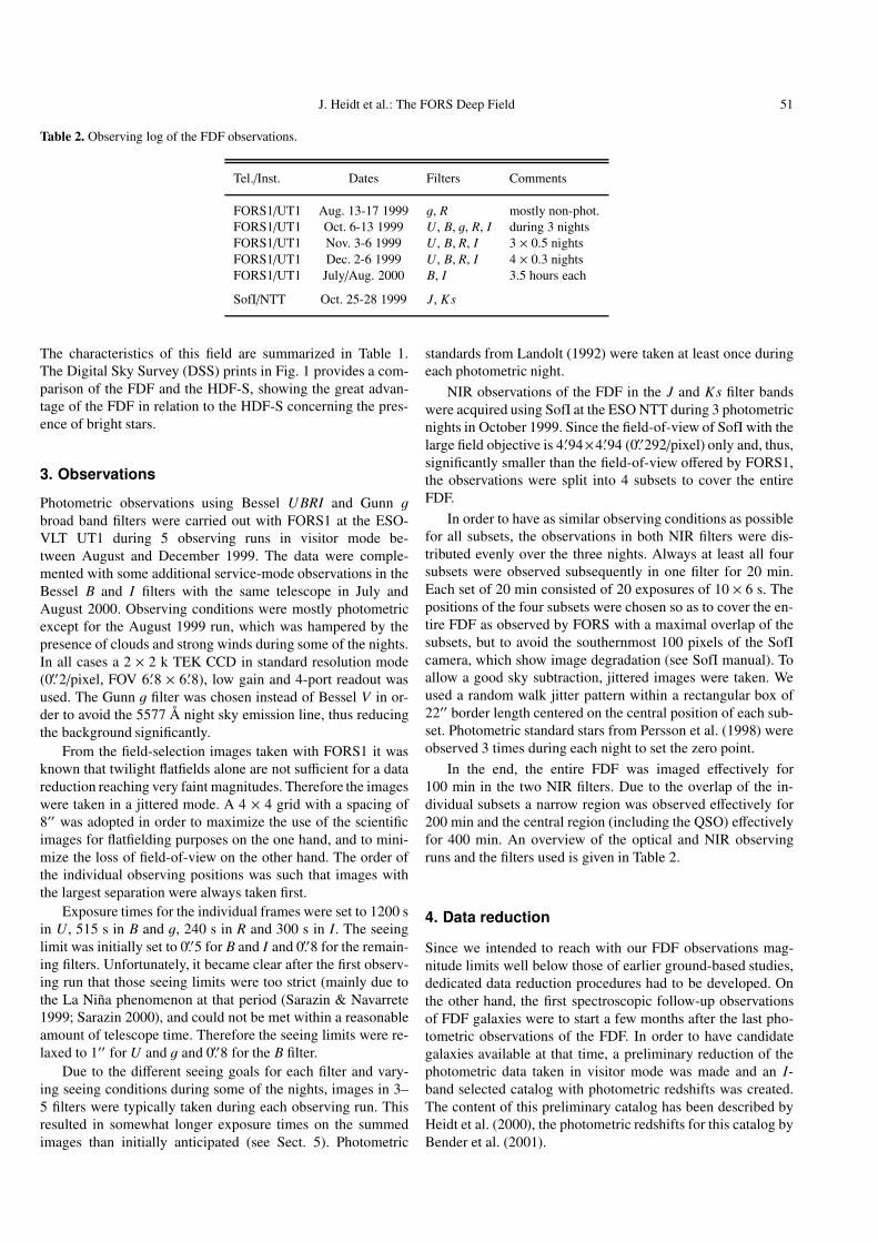
Table 2. Observing log of the FDF observations.

Tel./Inst. Dates Filters Comments

FORS1/UT1 Aug. 13-17 1999 g, R mostly non-phot.FORS1/UT1 Oct. 6-13 1999 U, B, g, R, I during 3 nightsFORS1/UT1 Nov. 3-6 1999 U, B, R, I 3 × 0.5 nightsFORS1/UT1 Dec. 2-6 1999 U, B, R, I 4 × 0.3 nightsFORS1/UT1 July/Aug. 2000 B, I 3.5 hours each

SofI/NTT Oct. 25-28 1999 J, Ks

The characteristics of this field are summarized in Table 1.The Digital Sky Survey (DSS) prints in Fig. 1 provides a com-parison of the FDF and the HDF-S, showing the great advan-tage of the FDF in relation to the HDF-S concerning the pres-ence of bright stars.

3. Observations

Photometric observations using Bessel UBRI and Gunn gbroad band filters were carried out with FORS1 at the ESO-VLT UT1 during 5 observing runs in visitor mode be-tween August and December 1999. The data were comple-mented with some additional service-mode observations in theBessel B and I filters with the same telescope in July andAugust 2000. Observing conditions were mostly photometricexcept for the August 1999 run, which was hampered by thepresence of clouds and strong winds during some of the nights.In all cases a 2 × 2 k TEK CCD in standard resolution mode(0.′′2/pixel, FOV 6.′8 × 6.′8), low gain and 4-port readout wasused. The Gunn g filter was chosen instead of Bessel V in or-der to avoid the 5577 Å night sky emission line, thus reducingthe background significantly.

From the field-selection images taken with FORS1 it wasknown that twilight flatfields alone are not sufficient for a datareduction reaching very faint magnitudes. Therefore the imageswere taken in a jittered mode. A 4 × 4 grid with a spacing of8′′ was adopted in order to maximize the use of the scientificimages for flatfielding purposes on the one hand, and to mini-mize the loss of field-of-view on the other hand. The order ofthe individual observing positions was such that images withthe largest separation were always taken first.

Exposure times for the individual frames were set to 1200 sin U, 515 s in B and g, 240 s in R and 300 s in I. The seeinglimit was initially set to 0.′′5 for B and I and 0.′′8 for the remain-ing filters. Unfortunately, it became clear after the first observ-ing run that those seeing limits were too strict (mainly due tothe La Nina phenomenon at that period (Sarazin & Navarrete1999; Sarazin 2000), and could not be met within a reasonableamount of telescope time. Therefore the seeing limits were re-laxed to 1′′ for U and g and 0.′′8 for the B filter.

Due to the different seeing goals for each filter and vary-ing seeing conditions during some of the nights, images in 3–5 filters were typically taken during each observing run. Thisresulted in somewhat longer exposure times on the summedimages than initially anticipated (see Sect. 5). Photometric

standards from Landolt (1992) were taken at least once duringeach photometric night.

NIR observations of the FDF in the J and Ks filter bandswere acquired using SofI at the ESO NTT during 3 photometricnights in October 1999. Since the field-of-view of SofI with thelarge field objective is 4.′94×4.′94 (0.′′292/pixel) only and, thus,significantly smaller than the field-of-view offered by FORS1,the observations were split into 4 subsets to cover the entireFDF.

In order to have as similar observing conditions as possiblefor all subsets, the observations in both NIR filters were dis-tributed evenly over the three nights. Always at least all foursubsets were observed subsequently in one filter for 20 min.Each set of 20 min consisted of 20 exposures of 10 × 6 s. Thepositions of the four subsets were chosen so as to cover the en-tire FDF as observed by FORS with a maximal overlap of thesubsets, but to avoid the southernmost 100 pixels of the SofIcamera, which show image degradation (see SofI manual). Toallow a good sky subtraction, jittered images were taken. Weused a random walk jitter pattern within a rectangular box of22′′ border length centered on the central position of each sub-set. Photometric standard stars from Persson et al. (1998) wereobserved 3 times during each night to set the zero point.

In the end, the entire FDF was imaged effectively for100 min in the two NIR filters. Due to the overlap of the in-dividual subsets a narrow region was observed effectively for200 min and the central region (including the QSO) effectivelyfor 400 min. An overview of the optical and NIR observingruns and the filters used is given in Table 2.

4. Data reduction

Since we intended to reach with our FDF observations mag-nitude limits well below those of earlier ground-based studies,dedicated data reduction procedures had to be developed. Onthe other hand, the first spectroscopic follow-up observationsof FDF galaxies were to start a few months after the last pho-tometric observations of the FDF. In order to have candidategalaxies available at that time, a preliminary reduction of thephotometric data taken in visitor mode was made and an I-band selected catalog with photometric redshifts was created.The content of this preliminary catalog has been described byHeidt et al. (2000), the photometric redshifts for this catalog byBender et al. (2001).


In a second step, all data including the photometric datataken in service mode were reduced as described below. Thisdata set forms the basis for the final photometric catalog de-scribed in the present paper.

4.1. Optical data

Because of the time variations of the CCD characteristics andof the telescope mirror (dust accumulation) each individual runwas reduced separately. However, in order to have a data setas homogeneous as possible, the data reduction strategy wasidentical for all 5 runs.

Firstly, the images were corrected for the bias. Since theobservations were done in 4-port readout mode, each port hadto be treated separately. A masterbias was formed for each portby the scaled median of typically 20 bias frames taken duringeach run, and subtracted from the images scaling the bias levelwith the overscan.

Next the images were corrected for the pixel-to-pixel vari-ations and large-scale sensitivity gradients. Since the twilightflatfields did not properly correct the large-scale gradients, acombination of the twilight flatfields and the science framesthemselves was used. The twilight flatfields taken in the morn-ing and evening generally differed considerably, and the twi-light flatfields always left large-scale gradients on the reducedscience frames (probably as a result of stray-light effects in thetelescope and the strong gradient of the sky background at thebeginning and the end of the night). Therefore, for each sci-ence frame, the sequence of flatfields was determined, whichminimized the large-scale gradient. These sequences were nor-malized, median filtered and used for 1st order correction ofthe pixel-to-pixel variations. Typically 2–3 flatfields per filterper run had to be created this way, leaving residuals of theorder of 2–8% (peak-to-peak) depending on the filter. To re-move the residuals, the twilight-flatfielded science frames weregrouped according to similar 2-dim large-scale residuals, nor-malized and stacked, using a 1.8 σ clipped median. Afterwardsa correction frame was formed by a 2−dim 2nd order polyno-mial fit to each median frame. This was done on a rectangulargrid of 50 × 50 points, where the level of each grid point wastaken as the median of a box with a width of 40 pixels. In thisway it was guaranteed that no residuals from stars affected thefit and a noise free correction frame was achieved. Finally, eachscience frame was corrected for the pixel-to-pixel variations bya combination of the corresponding twilight flatfield and noisefree correction frame. The peak-to-peak residuals on the finallyreduced science frames were typically 0.2% or less.

Cosmic ray events were detected by fitting a two-dimensional Gaussian to each local maximum in the frame. Allsignals with a FWHM smaller than 1.5 pixels and an ampli-tude >8 times the background noise were removed. Then thesepixels were replaced by the mean value of the surrounding pix-els. This provides a very reliable identification and cleaning ofcosmic ray events (for details see Gossl & Riffeser 2002).

In order to eliminate bad pixels and other affected regionsfor the image combination procedure, a bad pixel mask wascreated for every image. The positions of bad pixels on the

CCD were determined for each filter for each run using normal-ized flatfields. All pixels whose flatfield correction exceeded20% were flagged. Afterwards, each science frame was in-spected for other disturbed regions (satellite trails, border ef-fects) and their positions included in the corresponding badpixel masks.

The alignment of the images and the correction for the fielddistortion was done simultaneously. This ensured a minimiza-tion of smoothing and S/N reduction. As a reference frame,an I filter image of the FDF taken under the best seeing con-ditions in October 1999 was used. Depending on the filter,the positions of 15-25 reference stars were measured via aPSF fit on each frame. A linear coordinate transformation wasthen calculated to project the images with respect to the refer-ence image. The transformation included a rotation, a transla-tion and a global scale variation. Finally, the correction for thefield distortion was applied. Following the ESO FORS Manual,Version 2.4, we derive the FORS1 distortion corrected coordi-nates (x′, y′) in pixel units as a function of the distorted coordi-nates (x, y):

x′ = x − f (r)(x − x0), (1)

y′ = y − f (r)(y − y0), (2)

where (x0, y0) are the coordinates of the reference pixel, r =√(x − x0)2 + (y − y0)2 and

f (r) = 3.602 × 10−4 − 1.228 × 10−4 r + 2.091 × 10−9 r2. (3)

The flux interpolation for non-integer coordinate shifts was cal-culated from a 16-parameter, 3rd-order polynomial interpola-tion using 16 pixel base points (for details see Riffeser et al.2001). The same shifting procedure was applied to the corre-sponding bad pixel masks, flagging as “bad” every pixel af-fected by bad pixels in the interpolation.

The images were then co-added according to the followingprocedure: First, the sky value of each frame was derived via itsmode and subtracted. Then the seeing on each frame was mea-sured using 10 stars, and the flux of a non-saturated referencestar was determined. Next we assigned a weight to each imagerelative to the first image in each filter according to:

weight(n) =f (n)f (1)× h(1) FWHM(1)2

h(n) FWHM(n)2(4)

where n is the frame to be weighted relative to the 1st frame (1),f the flux of the reference star, h the sky level and FWHM theseeing on the frame. Weights computed according to Eq. (4)maximize the signal-to-noise ratio of the combined image forfaint ( f � h × FWHM2) point sources. These are the over-whelming majority of the objects studied here. Finally, theweighted sum was calculated and normalized to a 1 s expo-sure time. Pixels flagged as bad on the individual images werenot included in the coadding procedure. Since a different num-ber of dithered frames contributed to each pixel in the co-addedimages, producing a position-dependent noise pattern, a com-bined weight map to each frame was constructed. The latterwas included into the source detection and photometry proce-dure using SExtractor (see Sect. 6).


The photometric calibration of our co-added frames wasdone via “reference” standard stars in the FDF. We first deter-mined the zero points for two photometric nights (Oct. 10/11and 11/12, 1999) during which the FDF was imaged in all 5 op-tical filters. The colour correction and extinction coefficients onthe ESO Web-page were used to derive the zero points for ourFORS filter set in the Vega system. As no calibration imageswere available in the g-band, transformation from V to g wasperformed following Jørgensen (1994). We then convolved allthe FDF images from the two photometric nights to the sameseeing as the co-added frames and determined the magnitudesof 2 (U)–10 (I) stars. Based on a curve of growth for these stars,a fixed aperture with a diameter of 8′′ was used. Using thesereference stars, we finally determined the zero points of the co-added frames. The difference of the magnitudes between thereference stars on the individual frames on the two photomet-ric nights and on the co-added frames is 0.01 mag or less. Weverified our zero points by repeating the procedure describedabove using observations from two photometric nights duringour November 1999 run.

4.2. NIR data

About ∼10–20% of the observed NIR frames were found tocontain an electronic pattern caused by the fast motion of thetelescope near the zenith. These frames were excluded fromthe analysis. The remaining data were reduced using standardimage processing algorithms implemented within 1. Afterdark-subtraction, for each frame a sky frame was constructedtypically from the 10 subsequent frames which were scaled tohave the same median counts. These frames were then median-combined using clipping (to suppress fainter sources and other-wise deviant pixels) to produce a sky frame. The sky frame wasscaled to the median counts of each image before subtractionto account for variations of sky brightness on short time-scales.The sky-subtracted images were cleaned of bad-pixel defectsand flat-fielded using dome flats to remove detector pixel-to-pixel variations. The frames were then registered to high accu-racy, using the brightest ∼10 objects following the same proce-dure as described in the previous section, and finally co-added,after being scaled to airmass zero and an exposure time of 1 s.

The additionally observed photometric standard stars wereused to measure the photometric zero point. The typical for-mal uncertainties in the zero-points were 0.02 mag in J and0.01 mag in Ks.

5. Basic properties of the co-added images

A summary of the properties of the individual co-added imagesis presented in Table 3. The total integration time for the co-added images is given as well as the number of frames used,the average FWHM measured on 10 stars across the field, the

1 is distributed by the National Optical AstronomyObservatories, which are operated by the Association of Universitiesfor Research in Astronomy, Inc., under cooperative agreement withthe National Science Foundation.

area with 80% weight for each individual image and the 50%completeness limits for a point source as described in Sect. 6.

The integration times are in total almost a factor of 2 higherthan originally planned (except for the U filter). This is due toour strict seeing limits during the first observing runs. It com-pensates, at least in part, the loss of resolution/depth of the im-ages due to the less than optimal seeing. Still, the completenesslimits are somewhat lower than expected for the integrationtimes since the efficiencies of the telescope (reflectivity of themain mirror) and the CCD were below expected at the time ofthe observations. In general, the zero points remained relativelyconstant during the observations carried out in 1999, whereasthey differed considerably between the observations taken in1999 and 2000. This resulted in a loss of approx. 0.3 mag (seethe ESO-Web page, Paranal zero points).

The area with 80% weight is very similar for all opticalbands and 30% larger for the NIR bands. The latter is due tothe 4 subsets taken during the NIR observations. The commonarea with 80% weight in all filters is 39.′82.

As an example, the co-added I band image of the FDF isdisplayed in Fig. 2. The common area of the input images for a6′×6′ region is shown here. It contains ∼6100 galaxies. In gen-eral, the galaxies are distributed evenly across the field. Thereis a poor galaxy cluster (at z ∼ 0.3) in the southwestern cornerof the FDF. The QSO Q 0103-260 is south of the center of theframe and is marked with an arrow. The brightest object inthe field is an elliptical galaxy with mI = 16.5 at z ∼ 0.2 inthe southeastern part of the FDF.

6. Source detection and photometry

We used SExtractor (Bertin & Arnouts 1996) with theWEIGHT-IMAGE-option and WEIGHT-TYPE = MAP-WEIGHT for the source detection and extraction on the im-ages. The weight-maps described above were used to accountfor the spatial dependent noise pattern in the co-added images,and in particular to pass the local noise level of the data to theSExtractor program.

To use SExtractor, three parameters have to be set: i) Thedetection threshold t, which is the minimum signal-to-noise ra-tio of a pixel to be regarded as a detection, ii) the number nof contiguous pixels exceeding this threshold, iii) the filteringof the data prior to detection (e.g. with a top-hat or a Gaussianfilter). We used a Gaussian filter with a width θF , for the θFvalues see below.

We varied these parameters to maximize the number ofsource detections, while minimizing false detections. The fol-lowing procedure, described here for the I-band data, was usedfor all filters. We first considered only those pixels in the fieldwhere the exposure time equaled the total exposure time (theweight-map took care of the correct scaling of RMS for the fullfield later on) and called this part of data the “central field”.

If there were no objects in the field and if the data reductionresulted in a perfectly flat sky we would expect the histogramof the pixel-values to be a Gaussian, with a width reflectingthe photon-noise and the correlated noise of the data reduc-tion and coaddition procedure. The actual histogram of pixel-values of the central-field is shown in Fig. 3 (upper panel, thin


Table 3. Overview of the photometric observations.

Band Exposure Frames FWHM 80% weight 50% compl. limitTime [s] [′′] [′2] [mag]

U 44 400 37 0.97 40.7 25.64B 22 660 44 0.60 40.5 27.69g 22 145 43 0.87 41.1 26.86R 26 400 110 0.75 40.8 26.68I 24 900 83 0.53 40.9 26.37

J 4800a 80a 1.20 4.2/53.8 23.60/22.85Ks 4800a 80a 1.24 4.4/53.7 21.57/20.73

a Minimum exposure time and number of frames for each subset. Due to the overlap of the subsets for some (small) regions of the FDF the totaltime was twice or even four times this value. The 80% weight and 50% completeness levels in J and Ks are given for the 320 (central field)and 80-minutes co-added data, respectively.

line). Even ignoring the wings, the histogram is asymmetricaround its center at zero. This stems from the non-uniformitiesof the sky background, that amount to about 1% (see Sect. 4.1).Therefore, we determined the sky-curvature on large scales andsubtracted a 2-dimensional fit to this surface from the origi-nal data. The corrected histogram of pixel-values (Fig. 3, upperpanel, thick curve) is now symmetric around its center at zeroand the left-hand part is well described by a Gaussian (with awidth of 0.01295 ADU/s). The right hand part shows an ex-cess above ≈0.015 ADU/s, which is due to the objects in thefield (see difference curve in Fig. 3, scaled up by a factor 10).We have checked that it does not make any difference for thedetection and the photometry of reliable objects whether theprocedure is applied to the original or to the corrected data: foreach object, the difference between the magnitude estimates ofthese two cases is smaller than the assigned magnitude RMS-error. This implies that we can carry out the adjustment of op-timum SExtractor parameters in the corrected version of thedata.

To optimize the pre-detection filtering procedure we madethe following numerical experiment. We generated a “negativeversion” of an image by multiplying it by −1 and a “random-ized version” by randomly assigning measured pixel values tonew positions (the weights of the weight-map are re-localizedthe same way). With no filtering (θF = 0) and using t = 1.7 andn = 3 SExtractor finds about 9000 objects in the original image,5600 in the negative one and 1100 in the randomized one. Thefact that many more objects are detected in the negative imagethan in the randomized one indicates that correlated noise ispresent in both the negative and the positive images. Thereforefiltering must be used to specifically suppress the small-scalenoise. It is possible that large-scale noise is still present, butthere is no way to remove such a component. By varying thewidth θF of a Gaussian filter we found that θF = 2 is an optimalchoice. With n = 3 and t = 1.7 the number of objects detectedon the negative image dropped to the expected random number,nearly zero. Of course, once θF is fixed, one is still left with the

freedom of trading n for t by increasing the number of pixelsabove the threshold and decreasing the threshold value at thesame time. We decided to keep n small, in order to obtain anunbiased detection of faint point sources. This choice allowsus to exploit the excellent seeing of the I-band data, where theFWHM is only 2.5 pixels.

Now we illustrate our procedure more quantitatively: weran SExtractor (for each choice of θF , n and t) on the posi-tive, the negative and the randomized images. We registered allpixels which were covered by objects, removed them from thepixel-value statistics and normalized the corresponding pixel-value histogram to the total number of pixels in the centralfield, and we call that the “background-histogram”. We ex-pect that for good source extraction parameters, the backgroundhistograms will look like a Gaussian, more precisely like thatGaussian derived by fitting the negative wing of the correcteddata distribution, which we call the “optimum-background-histogram” below. The difference (magnified by a factor of 10)to that optimum background histogram is shown in the middlepanel of Fig. 3 for n = 3, t = 1.7, θF = 0 for detection onthe positive (solid) and negative (dotted, for negative ADU/sonly) image. The negative excess of these histograms belowzero are false detections due to correlated noise. Increasing θFthese false detections drop dramatically when θF = 2 pixels isreached. Then, n = 3 and t = 1.7 were fixed by requiring nofalse detections on the negative image, i.e. no detections dueto correlated noise. We finally run SExtractor with this set ofparameters on the positive image, obtain the background his-togram and show the difference to the optimum backgroundhistogram in the lower panel of Fig. 3 (dotted histogram, mag-nified by a factor of 10). The difference is indeed very small.

Using the above parameters (θF = 2 with a Gaussian con-volution, n = 3 and t = 1.7), obtained from the optimum pre-detection filtering and the requirement of no-detection on thenegative image, we find that the extended wing in the ADU-histogram due to the presence of objects disappears and thatthe histogram becomes symmetrical and Gaussian (see Fig. 3,


Fig. 2. The FDF in I band from FORS observations. The common area of all input frames for a field of view of 6′ × 6′ is shown here. North isup, east to the left. The total integration time was 6.9 h, mean FWHM ∼ 0.′′53. The QSO Q 0103-260 is south of the center of the frame andmarked with an arrow. This area contains ∼6100 galaxies. Note the even distribution of galaxies across the frame, except for the small galaxyconcentration in the southwestern corner. The brightest object in the field is the large elliptical galaxy in the southeastern part of the FDF atz ∼ 0.2 with mI = 16.5.

bottom panel). This demonstrates that with this choice of pa-rameters we are optimally extracting all objects above the noiselevel, without getting significant false detections. The adoptedparameters give a (total) photometric accuracy better than 5σ.

The optimum parameters were finally used to runSExtractor on the (positive and negative) images of the totalFDF. We found about 6900 objects on the positive and less thana handful of objects on the negative side of the entire I image.

All these spurious detections occurred near discontinuities ofthe S/N level outside the central field and were caused by thenon perfectly flat sky, which makes some of the discontinuitiesmore pronounced than they should be according to the photon-noise and the corresponding weight-map.

The same analysis described for the I-band image was car-ried out for the other filters. We emphasize here that our extrac-tion procedure was optimized to maximize the number of real


0 0.05

0

central field corrected central field

(corrected - gauss)x10

ADU/s

false detections and objects onpositive side, x10

-0.05 0 0.05 0.1

0

false detections onnegative side, x10

gauss fit to corrected data

ADU/s

-0.05 0 0.05 0.1

0

filtering applied

(filtering - gauss)x10

ADU/s

Fig. 3. Pixel-value histograms (in ADU per second) for the (central field) I image at various analysis stages. Upper panel: histogram of theoriginal data (thin line) and after subtracting the low frequency spatial variations due to the non-uniform sky background (thick line). Alsoincluded is the difference of the corrected histogram and a Gaussian (shown as thick line in the middle panel) fitted to its negative (ADU/s <0) wing. This negative wing should not be affected by real objects and therefore should represent the true noise in the image. For clarity thedifference has been scaled up by a factor of 10 and the curve has been labeled accordingly. The real objects show up as a positive excess of thepixel values in the corrected data distribution and in the difference function at positive ADU/s. Middle panel: the thick line shows the Gaussianderived by fitting the negative wing of the corrected data distribution as described above. Its difference to the pixel-value distribution derivedfor those pixels where SExtractor (with optimal parameters but without filtering) finds no objects (or object contributions) is shown as a solidline. The corresponding difference distribution of the inverted image is shown dotted for the negative ADU/s only. The negative excess showsthe false detections due to the correlated error. The difference curves are again scaled up by a factor of 10. Lower panel: the thin line showsthe histogram of the pixel values of pixels not belonging to objects when SExtractor is run after filtering the corrected data with a (2 pixelFWHM) Gaussian. The dotted line shows the difference between this histogram and the Gaussian fit shown in the middle panel. The number ofsignificant false detections has now dropped to nearly zero.

detections for a reliable photometry and hence reliable photo-metric redshifts rather than to study galaxy number counts atthe faintest limits. For the optical bands, we used the same ex-traction parameters. For the NIR-data we opted for θF = 3 pix-els to match the pixel size of the original NIR-data, which isroughly 1.5 the pixel size of FORS, and t = 2.0 and n = 5 forthe J band, and t = 1.9 and n = 5 for the Ks band, to takeinto account the poorer seeing and the different noise level. Toillustrate the reliability of our detection procedure we display adetection file returned from SExtractor for a 1′ × 1′ region ofthe northern part of the FDF in Fig. 4.

The photometric errors presented in the final catalog arethose derived by the SExtractor routine. To make sure thatthe error calculation was not influenced by correlated noise inthe sky background, the results of the SExtractor were veri-fied with aperture photometry with different apertures in areas

not covered by objects and by estimating the expected photo-metric errors from the background variations. In general wefound good agreement with the SExtractor derived errors. Inparticular the SExtractor errors were found to be quite accu-rate for point sources and for small objects. Only in the caseof large extended objects may non-stochastic background vari-ations have resulted in an underestimate of the photometric er-rors. But the few objects possibly affected are normally brightand have small errors, which should still be correct within thenumbers given in the catalog.

Finally, we calculated the 50% completeness levels in eachfilter band using our extraction parameters and the formulagiven in Snigula et al. (2002). This approach estimates the com-pleteness limit by calculating the brightness at which the areaof pixels brighter than the applied flux limit falls below the sizethreshold of the detection algorithm (for a given FWHM of a


Fig. 4. Detection file returned from SExtractor for a 1′ × 1′ region ofthe northern part of the FDF. It illustrates the reliability of our detec-tion and photometry procedure. The I-band image shown here con-tains ∼160 objects. For some objects the integrated magnitudes aredisplayed. The detection file shows the elliptical aperture limits usedto derive mag auto. Dashed ellipses denote blended objects.

point source). To allow a comparison with other deep fields,the data were corrected for galactic extinction as described inSect. 7. The results are summarized in Table 3.

7. Photometric catalog

7.1. Compilation of the photometric catalog

To create the final photometric catalog we merged the individ-ual catalogs of the objects detected in the co-added B filter im-age and in the co-added I filter image. We decided to use thesetwo catalogs as a basis, since the images in these two filterscorrespond to the best seeing conditions and since most typesof objects are expected to be detected in at least one of thesetwo bands.

The merging of the I and B catalogs was carried out as fol-lows: we first matched the positions of the detected objects andtheir corresponding images in the two filters. This was done byvisual inspection of the entries of the objects on both frames.This procedure gave us a clear view of the success of our au-tomatic detection procedure and allowed us to reject obviouslyfalse identifications. In order to avoid mis-matches in the finalcatalog, each entry in the B catalog was first assigned a corre-sponding entry in the I catalog and vice versa. A cross-match ofthe B versus I and I versus B entries allowed us to identify falsematches, which were checked again until a perfect cross-matchwas derived.

The initial catalogs in B and I contained 7206 and 6900 en-tries, respectively. After the visual cross-matching, we deleted

15 objects from the B catalog and 8 objects from the I catalog.These were mostly objects close to the edges of the field. In afew cases, 2 objects separated by a few pixels (e.g. a mergingpair of galaxies) were detected in the B band, whereas in theI band only one object in between the two B band objects wasfound (essentially at the center of the common envelope of bothgalaxies). In such cases the entry in the I band was deleted. Thisleft us with 7191 entries in the B catalog and 6892 entries in theI catalog. Now we merged both catalogs to form the final pho-tometric catalog. This catalog contains 8753 objects. 5327 outof the 8753 objects were detected in both filters (61%), whereas1864 (21%) were detected in B only and 1562 (18%) were de-tected in I only. We emphasize here that a non-detection doesnot necessarily mean that the object is not present on the frame,it rather means that the object was not detected by SExtractorwith the parameters set here.

Since SExtractor may use a different number of pixels toderive the total magnitudes in B and I, the colours of veryextended objects computed from the total magnitudes are notreliable. Therefore the catalog also contains aperture magni-tudes in UBgRIJKs. An aperture of 2′′ was chosen in orderto minimize the errors due to blending and since the faint ob-jects usually have diameters of ≤ 2′′. The aperture magnitudeswere derived by first convolving all frames to the same seeing(1′′ FWHM) and then performing aperture photometry on thepositions of the objects detected in B and I in the convolvedframes. For objects detected in B only, we used the aperturephotometry based on the positions in the B catalog, whereasthe aperture photometry based on the positions in the I catalogwere used for the remaining objects (detection on both framesor I-only detections). Thus for many objects, which were ini-tially not detected in either filter, useful photometric data couldbe given.

Finally, the galactic absorption towards the FORS DeepField was estimated. We used the formulae 2 and 3 in Cardelliet al. (1989) and adopted E(B−V) = 0.018 (Burstein & Heiles1982) and AV = 3.1 × E(B − V) to calculate the extinctioncorrection for each filter. The central wavelengths for each fil-ter were taken from the ESO Web-page. We derived AU/AV =

1.555, AB/AV = 1.365, Ag/AV = 1.105, AR/AV = 0.790,AI/AV = 0.631, AJ/AV = 0.283 and AKs/AV = 0.117 result-ing in AU = 0.087 mag, AB = 0.076 mag, Ag = 0.062 mag,AR = 0.041 mag, AI = 0.035 mag, AJ = 0.016 mag andAKs = 0.007 mag, respectively. The values for the extinctionagree to ≤0.01 mag with those listed in the NED. The pho-tometric catalog described below is not corrected for galacticextinction. However, the completeness limits as well as thenumber counts shown in Sect. 8 were derived with a galacticextinction correction.

7.2. Contents of the photometric catalog

The full catalog containing 8753 objects is avail-able in electronic form at CDS via anonymous ftpto cdsarc.u-strasbg.fr (130.79.128.5) or viahttp://cdsweb.u-strasbg.fr/cgi-bin/qcat?J/A+A/398/49.


As an illustration of its content we list in Table 4 the entries2630−2639.

For each object we report the following parameters:ID: the identification number. The objects have been sorted

first by right ascension (2000), followed by declination (2000).The identification numbers provide a cross-reference to thespectroscopic and other observations of the FDF (e.g. Nollet al., in prep.).

RA, Dec: the positions of the objects in the FDF forJ2000.0. Their accuracy has been examined by comparing thepositions of 31 well-isolated, evenly distributed objects on theI frame of the FDF, to those listed in the USNO catalog (Monet1998). The mean difference in right ascension is 0.′′21 ± 0.′′38and the mean difference in declination is 0.′′14 ± 0.′′40. Given atypical accuracy of 0.′′25 for objects in the USNO catalog ourpositions have an accuracy of ∼0.′′5.

mBT, σBT, mIT,σIT: the total magnitudes (Vega-system) andassociated mean errors of the detected sources in the B and Iband images, respectively, as measured using the SExtractorroutine mag auto on the co-added and unconvolved frames.Mag auto is an automatic aperture routine based on Kron’s(1980) “first moment” algorithm, which determines the sum ofcounts in an elliptical aperture. The semimajor axis of this aper-ture is defined by 2.5 times the first moments of the flux dis-tribution within an ellipse roughly twice the isophotal radius,within a minimum semimajor axis of 3.5 pixels. This routineis intended to give the most precise estimate of “total magni-tudes”, at least for galaxies, and takes into account the blendingof nearby objects.

mUBgRIJKs[2′′], σUBgRIJKs: UBgRIJKs magnitudes (Vega-System) and associated errors within an aperture of 2′′. They(and their errors) were measured on the co-added and con-volved frames using SExtractor. The positions listed in the cat-alog were used for this procedure. An aperture of 2′′ was cho-sen in order to minimize the errors due to blending. Moreover,the faint objects in the FDF usually have diameters of ≤2′′.Choosing a larger aperture would result in larger photometricerrors due to the sky background. For extended objects, themean errors of the aperture magnitudes are generally smallerthan for the total magnitudes, as the aperture photometry se-lected the regions of high surface brightness. The magnitudeswere not corrected for blending. Blended objects can be iden-tified from the column Flag1 (see below).

The next four columns (FWHM, elongation, positionangle, star-galaxy classification parameter) describe the mor-phology of the objects. Since the FWHM, elongation and po-sition angle may have high errors and are sometimes unreli-able for faint objects, this information is provided for objectsbrighter than our 50% completeness limit (27.69 in B, 26.37in I) only. Moreover, we do not list these values for objectswhere SExtractor derived a FWHM < 0.′′4 (FWHM is 0.′′53 inco-added I band frame and 0.′′6 in co-added B band frame). Theinformation should also be treated with caution for brighter ob-jects having a star-galaxy classification parameter >0.9.

FWHM: Full width at half maximum of the objects in arc-sec as determined by SExtractor by a Gaussian fit to the core.

Elong: Elongation of the images. The elongation is definedas A/B, where A and B are given by the 2nd order moment of

the light distribution along the major and minor axis, respec-tively.

PA: The position angle of the major axis, measured fromNorth to East, with N-S = 0.

Cstar: Star-galaxy classification parameter returned bySExtractor based on the morphology of the objects on theimage. A classification near 1.0 describes point like sourceswhereas a classification close to 0.0 describes extendedsources.

Flag1: flags returned by SExtractor with the followingnotation:1: object has neighbours bright and close enough to bias sig-nificantly mag auto; 2: the object was originally blended withanother one; 3: sum of 1 + 2; 4: at least one pixel of the objectis saturated (or very close to saturation); 7: sum of 1 + 2 + 4; 8:the object is truncated (e.g. too close to the image boundary);16: object aperture data are incomplete or corrupted; 17: sumof 1 + 16; 18: sum of 2 + 16; 19: sum of 1 + 2 + 16; 24: sumof 8 + 16.

Flag2: here we report if an object was detected on the Bframe only (“Bonly”), on the I frame only (“Ionly”). If there isno entry, the object is detected by SExtractor on both frames.

Flag3: a preliminary classification of 35 point-like objects(QSOs, stars) from our spectroscopic survey (Noll et al., inprep.).

weight B, weight I: averaged weights of all pixels used todetermine mBT and mIT, respectively. They were derived fromthe combined weight maps which are described in Sect. 4. Aweight of 1 means that all pixels used to derive the magnitudeare fully exposed and not affected by bad areas. Most of thedetections with low weights are close to the edges of the FDFwhere the total integration times are lower.

8. Galaxy number counts

The number counts serve as a quick check of the approxi-mate photometric calibration and for the depth of the data. Wedid not put much effort in star-galaxy separation at the faintend, where the galaxies dominate the counts anyway. At thebright end, where SExtractor is able to disentangle a stellarand a galaxy profile, we derived limits by investigating theclass-FWHM diagram for the objects. In the following fig-ures, the counts for all objects are shown as dashed histograms,while for the solid line histograms obvious stellar objects havebeen omitted. The magnitudes are given in the Vega-system.The number counts are given only for the area with maximumintegration-times (weight-map ≈1) for the optical data and forweight −map >∼ 0.25 for the NIR-data (i.e. we exclude theedges of the fields). They are not corrected for incompleteness.Also indicated is the 50% completeness limit for the detectionof point sources. For each filter we also included for compar-ison number-magnitude-relations obtained in earlier observa-tions which are compiled and transformed to standard filtersystems in Metcalfe et al. (2001) for the optical filters. In allcases we plot raw number counts only, i.e. we do not correctfor incompleteness at the faint end.

In the U-band the FDF is 50% complete to U = 25.64mag for a point source. The slope agrees with earlier mea-


Table 4. Excerpt from the FDF object catalog. The entries with the IDs 2630−2639 are displayed as examples.

ID RA (2000) Dec (2000) mBT σBT mIT σIT mU [2′′] σU mB [2′′] σB mg [2′′] σg mR [2′′] σR mI [2′′] σI

2630 1 5 57.28 −25 48 02.3 27.75 0.19 25.30 0.10 26.99 0.27 27.61 0.05 27.72 0.10 26.10 0.03 25.34 0.022631 1 5 57.29 −25 45 00.1 24.42 0.03 30.73 1.65 26.57 0.04 24.49 0.012632 1 5 57.29 −25 48 46.9 26.13 0.05 24.98 0.07 25.96 0.10 26.20 0.01 25.92 0.02 25.42 0.02 25.05 0.022633 1 5 57.30 −25 44 56.6 24.47 0.01 22.75 0.01 24.60 0.03 24.60 0.01 23.74 0.01 23.26 0.01 22.87 0.012634 1 5 57.30 −25 48 14.2 27.69 0.16 27.77 0.06 28.23 0.17 26.84 0.06 26.78 0.092635 1 5 57.31 −25 43 52.3 25.02 0.09 26.22 0.13 26.42 0.02 26.11 0.02 25.66 0.02 25.33 0.022636 1 5 57.31 −25 44 02.2 24.85 0.04 23.43 0.04 25.53 0.07 25.53 0.01 25.12 0.01 24.56 0.01 24.12 0.012637 1 5 57.31 −25 44 15.2 26.60 0.09 26.19 0.17 26.76 0.22 26.83 0.02 26.72 0.04 26.46 0.04 26.16 0.052638 1 5 57.31 −25 46 23.5 27.36 0.16 25.65 0.09 27.58 0.46 27.43 0.04 27.45 0.08 26.72 0.05 25.67 0.032639 1 5 57.31 −25 47 51.1 26.17 0.08 25.11 0.10 26.42 0.16 26.85 0.02 26.74 0.04 26.22 0.03 25.60 0.03

ID mJ [2′′] σJ mKs [2′′] σKs FWHM [′′] Elong PA [◦] Cstar Flag1 Flag2 Flag3 weight B weight I

2630 21.97 0.20 0.74 1.17 17.9 0.40 0 1.000 1.0002631 21.36 0.01 20.35 0.03 0.52 1.02 111.7 0.98 0 Ionly L star 1.0002632 26.58 2.38 22.37 0.29 0.78 1.12 82.1 0.26 0 1.000 1.0002633 22.09 0.03 20.91 0.06 0.53 1.04 36.2 0.98 0 QSO 1.000 1.0002634 1.01 1.25 00.6 0.61 0 Bonly 1.0002635 23.70 0.18 1.13 1.19 129.3 0.00 3 Ionly 0.9842636 22.71 0.07 20.75 0.07 0.73 1.34 90.2 0.09 3 0.984 1.0002637 1.07 1.87 76.9 0.40 0 1.000 1.0002638 0.80 1.49 19.1 0.43 0 1.000 1.0002639 24.02 0.23 22.96 0.50 1.34 1.16 21.6 0.01 2 1.000 1.000

Hogg et al. 1997

Metcalfe et al. 2001, WHDF

Metcalfe et al. 2001, HDFS

Metcalfe et al. 2001, HDFN

Fig. 5. Galaxy number counts of the FDF in the U band (not correctedfor incompleteness) as compared to other deep surveys. The verticaldash-dotted line indicates the 50% completeness limits.

surements (roughly 0.4−0.5) for U < 23 and it becomes shal-lower (0.35 at U = 23−25), in agreement with the slopes ofthe HDF-S, WHDF and Hogg et al. (1997) (see Metcalfe et al.2001). In Fig. 5 we have transformed the HDF number countsas proposed by Metcalfe et al. using F3oo,Vega = U − 0.4 andTable 5 in their paper. We further assume UWHDF ≈ U to in-

Arnouts et al. 1999, NTTDF

Metcalfe et al. 2001, WHDF+INT



Fig. 6. Galaxy number counts of the FDF in B band (not correctedfor incompleteness) as compared to other deep surveys. The verticaldash-dotted line indicates the 50% completeness limits.

clude the WHDF U-band-raw counts (Table 4 of Metcalfe et al.2001) – in fact the central wavelengths and the transmissioncurves of the U filters used for the FDF and WHDF observa-tions are similar. The values of Hogg et al. (1997) have beenobtained from their Fig. 3 and been transformed as proposedby Metcalfe, U ≈ UHogg + 0.08. The HDFN/S and WHDF


Arnouts et al. 1999, NTTDF


Bertin & Dennefeld 1997



Metcalfe et al. 1995

Metcalfe et al. 1991

Hogg et al. 1997

Fig. 7. Galaxy number counts of the FDF in R band (not correctedfor incompleteness) as compared to other deep surveys. The verticaldash-dotted line indicates the 50% completeness limits.

Huang et al. 1998

Williams et al. 1996




Fig. 8. Galaxy number counts of the FDF in I band (not corrected forincompleteness) as compared to other deep surveys. The vertical dash-dotted line indicates the 50% completeness limits.

number counts are not corrected for reddening (Metcalfe, pri-vate comm., E(B− V)WHDF ≈ 0.02 which is similar to the FDFand thus would shift the number counts by ≈−0.1).

Our B-band number counts (Fig. 6) are 50%-complete at27.69 mag. Within the field-to-field variations they agree wellwith the HDFS/N (we follow Metcalfe et al. (2001) and use thetransformation F450,Vega ≈ B − 0.1) and the raw-counts in theNTT deep field (Arnouts et al. 1996). We also included the rawcounts in the Herschel deep field, assuming BFDF ≈ BWHDF.

For the g-band, we just show our results in Fig. 10 withoutcomparison, since no adequate number counts have been pre-sented in the literature for this passband. Our estimated 50%completeness limit is 26.86 mag in this filter.

Our R-band and I-band data are 50%-complete at26.68 mag and 26.37 mag, respectively. Amplitude andslope agree well with previously published fields. For the

Teplitz et al. 1999

Saracco et al 1999

Bershady 1998

Fig. 9. Galaxy number counts of the FDF in J band (not corrected forincompleteness) as compared to other deep surveys. The vertical solidline indicates the 50% completeness for the shallower exposed partof the field, whereas the vertical dash-dotted line indicates the 50%completeness for the deeply exposed part of the field.

Fig. 10. Galaxy number counts of the FDF in g band (not correctedfor incompleteness). The vertical dash-dotted line indicates the 50%completeness limits.

transformation of the HDF-counts we followed Metcalfe et al.2001) and used R ≈ R606,Vega − 0.1 and I ≈ I814,Vega; we also as-sumed that R ≈ RWHDF. The counts are shown in Figs. 7 and 8.

Our number counts in the J-band (Fig. 9) agree with thosederived by Saracco et al. (1999), and precisely match thoseof Teplitz et al. (1999). The completeness is 22.85 mag and23.60 mag for the shallower and deeply exposed (factor of fourin integration time) part of the field, respectively. Our num-ber counts in the K-band (Fig. 11) agree well with those ofKummel & Wagner (2001) and Huang et al. (1998). The com-pleteness limits are 20.73 mag and 21.57 mag for the shallowand deep exposed part of the field. For fairly shallow J and Kpointings (J <∼ 22 and K <∼ 20) the field-to-field variations are


Cowie 1994

Kuemmel 2001

Huang 2001

Fig. 11. Galaxy number counts of the FDF in Ks band (not correctedfor incompleteness) as compared to other deep surveys. The verticalsolid line indicates the 50% completeness for the shallower exposedpart of the field, whereas the vertical dash-dotted line indicates the50% completeness for the deeply exposed part of the field.

expected to be significant for our field size, since the distribu-tion of massive, old systems dominating the NIR frames variesconsiderably on small scales. This has been demonstrated e.g.in the different pointings of the MUNICS survey by Droryet al. (2001). The agreement with other surveys is good andthe quoted detection limit correspond to the 50% completenesslimit of our sample.

Acknowledgements. We thank the Paranal and NTT staff at ESO fortheir excellent and very efficient support at the telescope. We alsothank the referee (Dr. M. Franx) for his constructive comments. Thiswork has been supported by the Deutsche Forschungsgemeinschaft(SFB 375, SFB 439), the VW foundation (I/76520) and the GermanFederal Ministry of Science and Technology (Grants 05 2HD50A, 052GO20A and 05 2MU104).

We have made use of the Simbad Database, operated at CDS,Strasbourg, France, and the NASA/IPAC Extragalactic Database(NED), operated by the Jet Propulsion Laboratory, California insti-tute of Technology under contract with the National Aeronautics andSpace Administration.

References

Appenzeller, I., Fricke, K., Furtig, W., et al. 1998, The Messenger,94, 1

Appenzeller, I., Mehlert, D., Noll, S., et al. 2002, High redshift galax-ies in the FORS Deep Field; in Studies of Galaxies in the YoungUniverse with New Generation Telescopes, ed. N. Arimoto, ADSElectronic Publications 2002, in press

Arnouts, S., D’Odorico, S., Cristiani, S., et al. 1999, A&A, 341, 641Bender, R., Appenzeller, I., Bohm, A., et al. 2001, The FORS Deep

Field: Photometric redshifts and object classification, in DeepFields, ed. S. Cristiani, A. Renzini, & R. E. Williams, ESO as-trophysics symposia (Springer), 96

Bershady, M. A., Lowenthal, J. D., Koo, D. C. 1998, ApJ, 505, 50Bertin, E., & Arnouts, S. 1996, A&AS, 117, 393Bertin, E., & Dennefeld, M. 1997, A&A, 317, 43Burstein, D., Heiles, C. 1982, AJ, 87, 1165Cardelli, J. A., Clayton, G. C., Mathis, J. S. 1989, ApJ, 345, 245Cohen, J. G. 1998, Redshift clustering in the Hubble Deep Field; in

The Hubble Deep Field, ed. M. Livio, S. M. Fall, & P. Madau,STScI Symposium Series, 11, 52

Connolly, A. J., Szalay, A. S., Dickinson, M., Subbaro, M. U.,Brunner, R. J. 1977, ApJ, 486, L11

Cowie, L. L., Gardner, J. P., Hu, E. M., et al. 1994, ApJ, 434, 114Drory, N., Feulner, G., Bender, R. 2001, MNRAS, 325, 550Gossl, C. A., & Riffeser, A. 2002, A&A, 381, 1095Heidt, J., Appenzeller, I., Bender, R., et al. 2000, Rev. Mod. Astr., 14,

209Hogg, D. W., Pahre, M. A., McCarthy, J. K., et al. 1997, MNRAS,

288, 404Huang, J.-S., Cowie, L. L., & Luppino, G. A. 1998, ApJ, 496, 31Huang, J.-S., Thompson, D., Kummel, M. W., et al. 2001, A&A, 370,

909Jørgensen, I. 1994, PASP, 106, 967Kajisawa, M., & Yamada, T. 2001, PASJ, 53, 833Kron, R. G. 1980, ApJS, 43,305Kummel, M. W., & Wagner, S. J. 2001, A&A, 370, 384Jager, K., Heidt, J., Appenzeller, I., et al. 1999, The FORS Deep Field

(FDF): Selection and first impressions, AG Abstr. Ser., 15, 43Landolt, A. U. 1992, AJ, 104, 340Mehlert, D., Noll, S., Appenzeller, I., et al. 2001, The FORS Deep

Field: First spectroscopic results; in Deep Fields, ed. S. Cristiani,A. Renzini, & R. E. Williams, ESO astrophysics symposia(Springer), 162

Mehlert, D., Noll, S., Appenzeller, I., et al. 2002, A&A, 393, 809Meisenheimer, K., Beckwith, S., Fockenbrock, R., et al. 1998, The

Calar Alto Deep Imaging Survey (CADIS); in The young uni-verse: galaxy formation and evolution at intermediate and highredshift, ed. S. O’Dorico, A. Fontana, & E. Giallongo, ASP Conf.Ser., 136, 134

Metcalfe, N., Shanks, T., Fong, R., & Jones, L. R. 1991, MNRAS,249, 498

Metcalfe, N., Shanks, T., Campos, A., McCracken, H. J., & Fong, R.2001, MNRAS, 323, 795

Monet, D. G. 1998, BAAS, 193, 120.03Noll, S., Mehlert, D., Appenzeller, I., et al. 2001, Spectroscopy in the

FORS Deep Field, AG Abstr. Ser., 18, 57Persson, S. E., Murphy, D. C., Krzeminski, W., Roth, M., Rieke, M. J.

1998, AJ, 116, 2475Riffeser, A., Fliri, J., Gossl, C. A., et al. 2001, A&A, 379, 362Saracco, P., D’Odorico, S., Moorwood, A., et al. 1999, A&A, 349, 751Sarazin, M., & Navarrete, J. 1999, The Messenger, 97, 8Sarazin, M. 2000, The Messenger, 99, 13Snigula, J., Drory, N., Bender, R., et al. 2002, MNRAS, submittedTeplitz, H. I., McLean, I. S., & Malkan, M. A. 1999, ApJ, 520, 469Tyson, J. A. 1988, AJ, 96, 1Veron-Cetty, M. P., & Veron, P. 1997, A catalog of Quasars and Active

Nuclei (7th edn.)Warren, S. J., Hewett, P. C., & Osmer, P. S. 1991, ApJS, 76, 23Williams, R. E., Blacker, B., Dickinson, M., et al. 1996, AJ, 112, 1335Williams, R. E., Baum, S., Bergeron, L., et al. 2000, AJ, 120, 2735Ziegler, B. J., Bohm, A., Fricke, K. J., et al. 2002, ApJ, 564, L69

the fors deep field: field selection, photometric ... filee-mail: [email protected] based...

Documents