Louisiana State UniversityLSU Digital Commons

LSU Historical Dissertations and Theses Graduate School

1986

The Fricative Sound Source Spectrum DerivedFrom a Vocal Tract Analog.Lawrence Edward ZagarLouisiana State University and Agricultural & Mechanical College

Follow this and additional works at: https://digitalcommons.lsu.edu/gradschool_disstheses

This Dissertation is brought to you for free and open access by the Graduate School at LSU Digital Commons. It has been accepted for inclusion inLSU Historical Dissertations and Theses by an authorized administrator of LSU Digital Commons. For more information, please contactgradetd@lsu.edu.

Recommended CitationZagar, Lawrence Edward, "The Fricative Sound Source Spectrum Derived From a Vocal Tract Analog." (1986). LSU HistoricalDissertations and Theses. 4275.https://digitalcommons.lsu.edu/gradschool_disstheses/4275

INFORMATION TO USERS

This reproduction was made from a copy of a manuscript sent to us for publication and microfilming. While the m ost advanced technology has been used to pho­tograph and reproduce this manuscript, the quality of the reproduction is heavily dependent upon the quality of the material submitted. Pages in any m anuscript may have indistinct print. In all cases the best available copy has been filmed.

The following explanation of techniques is provided to help clarify notations which may appear on this reproduction.

1. Manuscripts may not always be complete. When it is not possible to obtain missing pages, a note appears to indicate this.

2. When copyrighted materials are removed from the manuscript, a note ap­pears to indicate this.

3. Oversize materials (maps, drawings, and charts) are photographed by sec­tioning the original, beginning at the upper left hand comer and continu­ing from left to right in equal sections with small overlaps. Each oversize page is also filmed as one exposure and is available, for an additional charge, as a standard 35mm slide or in black and white paper format.*

4. Most photographs reproduce acceptably on positive microfilm or micro­fiche bu t lack clarity on xerographic copies made from the microfilm. For an additional charge, all photographs are available in black and white standard 35mm slide format. *

*For more information about black and white slides or enlarged paper reproductions, please contact the Dissertations Customer Services Department

T TA/FT Dissertation \J 1 V 1 1 Information ServiceUniversity Microfilms internationalA Bell & Howell Information Company300 N. Zeeb Road, Ann Arbor, Michigan 48106

8629209

Z agar, L aw re n c e E dw ard

THE FRICATIVE SOUND SOURCE SPECTRUM DERIVED FROM A VOCAL TRACT ANALOG

The Louisiana State University and Agricultural and Mechanical Col. Ph.D. 1986

UniversityMicrofilms

International 300 N. Zeeb Road, Ann Arbor, Ml 48106

PLEASE NOTE:

In all cases this material has been filmed in the best possible way from the available copy. Problems encountered with this docum ent have been identified here with a check mark V .

1. Glossy photographs or p a g e s_____

2. Colored illustrations, paper or p rin t_______

3. Photographs with dark background_____

4. Illustrations are poor copy_______

5. Pages with black marks, not original copy______

6. Print shows through as there is text on both sides of p a g e _______

7. indistinct, broken or small print on several pages

8. Print exceeds margin requirem ents______

9. Tightly bound copy with print lost in sp in e_______

10. Computer printout pages with indistinct print_______

11. Page(s)_____________lacking when material received, and not available from school orauthor.

12. Page(s)_____________seem to be missing in numbering only as text follows.

13. Two pages num bered . Text follows.

14. Curling and wrinkled p a g e s_______

15. Dissertation con tains pages with print a t a slant, filmed a s received_________

16. Other________ _________________________________________________ __________

UniversityMicrofilms

International

THE FRICATIVE SOUND SOURCE SPECTRUM DERIVED FROM A

VOCAL TRACT ANALOG

A DissertationSubmitted to the Graduate Faculty of the

Louisiana State University and Agricultural and Mechanical College

in partial fulfillment of the requirements for the degree of

Doctor of Philosophyin

Mechanical Engineering

by Lawrence E. Zagar B.S., Louisiana State University, 1981 M.S., Louisiana State University, 1983

May 1986

ACKNOWLE DGEMENTS

This dissertation could not have been completed without the help of many people. The author wishes to thank these people at this time.

First the author wishes to thank his majorprofessors Dr. G. D. Catalano and Dr. J. K. Thompson for all the assistance, guidance, and encouragement they offered. The author is alsoindebted to the members of his committee, Dr. J. A. Brewer, Dr. V. A. Cundy, Dr. S. S. Iyengar, Dr. D. M. Klein, Dr. D. E. Thompson, for theirservice. Appreciation is given to Dr. A. R. P. Rau who was appointed as an observer during the defense of this dissertation.

Special thanks are given to the author's wife whose compassion and understanding were unparalleled. The author appreciates all the time and effort hissister contributed towards the construction of the figures presented in this dissertation. The author also asks forgiveness of his newly born daughter for missing out on the many milestones she has achieved during the writing of this dissertation.

i i

Thanks are given to Ric Haag, the author's office mate. Ric is the systems manager of the Computer Graphics Research and Applications Laboratory (CGRAL). The computing facilities of CGRAL were used both for the computations of this dissertation and its writing. Ric's help in the use of the computing facilities and the permission to use these facilities are appreciated.

Lastly, the author thanks The Goodyear Tire and Rubber Company for allowing the author to use their semi-anechoic chamber and instrumentation for the experimental part of this dissertation. The forgiveness of anyone not acknowledged and who are deserving is requested.

TABLE OF CONTENTSPage

ACKNOWLEDGEMENTS........................... iiLIST OF TABLES.................................... viLIST OF FIGURES................................... viiABSTRACT........................................... xiNOMENCLATURE...................................... xiii1. INTRODUCTION................................... 12. REVIEW OF SPEECH SYNTHESIS ANDISOTROPIC TURBULENCE............................. 4

2.1 Speech Synthesis......................... 4Vocal Tract Analog.................. 4Excitation Sources.................. 12Formant Synthesis.................... 24Digital Storage and Playback......... 28Linear Predictive Coding............ 32Fricatives........................... 35

2.2 Isotroic Turbulence...................... 373. ANALYTICAL DEVELOPMENT........................ 47

Vocal Tract Analog........................... 49Vocal Tract Areas............................ 61Computer Program and Logic.................. 64Fourier Series................................ 71

4. EXPERIMENTAL MEASUREMENTS.................... 72Experimental Procedure....................... 72Data........................................... 77

5. THE FRICATIVE SOURCE SPECTRA................. 91Results......... 91Turbulence.................................... 118Model.......................................... 124

6. CONCLUSIONS AND RECOMMENDATIONS.............. 139Conclusions................................... 139Recommendations............................... 140

7. BIBLIOGRAPHY.................................. 143iv

PageAPPENDICES........................................ 150

Appendix I: Vocal Tract Area Functions..... 151Appendix II: Computer Program Listing...... 157Appendix III: Coefficients of Model........ 161

VITA............................................... 172

v

LIST OF TABLESTable Page1. Vocal Tract Area for /f/....................... 1522. Vocal Tract Area for /th/...................... 1533. Vocal Tract Area for /s/....................... 1544. Vocal Tract Area for /sh/...................... 1555. Vocal Tract Area for /h/....................... 1566. Fourier Coefficients for Source Spectrumof /f/ Obtained from Pressure Measurement........ 1627. Fourier Coefficients for Source Spectrum of /f/ Obtained fromIntensity Measurement Technique.................. 1638. Fourier Coefficients for Source Spectrumof /th/ Obtained from Pressure Measurement ..... 1649. Fourier Coefficients for Source Spectrum of /th/ Obtained fromIntensity Measurement Technique.................. 16510. Fourier Coefficients for Source Spectrumof /s/ Obtained from Pressure Measurement ...... 16611. Fourier Coefficients for Source Spectrum of /s/ Obtained fromIntensity Measurement Technique.................. 16712. Fourier Coefficients for Source Spectrumof /sh/ Obtained from Pressure Measurement...... 16813. Fourier Coefficients for Source Spectrum of /sh/ Obtained fromIntensity Measurement Technique.................. 16914. Fourier Coefficients for Source Spectrumof /h/ Obtained from Pressure Measurement........ 17015. Fourier Coefficients for Source Spectrum of /h/ Obtained fromIntensity Measurement Technique.................. 171

vi

LIST OF FIGURES Figure Page1. Equivalent Electrical Circuit for Vocal Tract

Tube Section.................................... 72. Lumped Parameter Equivalent Circuit for Soft

Vocal Tract Tube Section....................... 133. Spectrum of the Glottal Turbulent Noise

Source from Hillman et al [11]................ 244. Subdivision of Energy Spectrum for Turbulent

Flows with Large Reynolds Number.............. 445. Two Mass Model of the Vocal Cords............ 586. Equivalent Circuit of Vocal Tract Showing

Fricative Source Locations.................... 607. Computer Program Flowchart.................... 658. Symbolic Matrix that Displays the

Segmentation of Zeros in the Off Diagonals... 689. Inverse Filter Function for Vowel "a" with

High Resistive Glottal Impedance............. 7010. Schematic of the Instrumentation Used in

Making the Experimental Measurements.......... 7311. Two Microphone Measurement Apparatus......... 7612. Spectrum of the Sound Pressure for /f/

Obtained from Pressure Measurement............ 7813. Spectrum of the Sound Pressure for /f/

Obtained by Intensity Measurement Technique... 7914. Spectrum of the Sound Pressure for /th/

Obtained from Pressure Measurement............ 8015. Spectrum of the Sound Pressure for /th/

Obtained by Intensity Measurement Technique... 8116. Spectrum of the Sound Pressure for /s/

Obtained from Pressure Measurement........... 83vii

Figure Page17. Spectrum of the Sound Pressure for /s/

Obtained by Intensity Measurement Technique.. 8418. Spectrum of the Sound Pressure for /sh/

Obtained from Pressure Measurement............ 8619. Spectrum of the Sound Pressure for /sh/

Obtained by Intensity Measurement Technique.. 8720. Spectrum of the Sound Pressure for /h/

Obtained from Pressure Measurement............ 8821. Spectrum of the Sound Pressure for /h/

Obtained by Intensity Measurement Technique.. 8922. Sound Pressure Level Spectrum of the Source

for /f/ Derived from Pressure Data. Source Location Downstream of the Constriction..... 92

23. Sound Pressure Level Spectrum of the Source for /f/ Derived from Pressure Data. Source Location at the Constriction................. 93

24. Sound Pressure Level Spectrum of the Source for /f/ Derived from Intensity Data. Source Location Downsteam of the Constriction...... 94

25. Sound Pressure Level Spectrum of the Source for /f/ Derived from Intensity Data. Source Location at the Constriction...... 95

26. Sound Pressure Level Spectrum of the Source for /th/ Derived from Pressure Data. Source Location Downstream of the Constriction..... 97

27. Sound Pressure Level Spectrum of the Source for /th/ Derived from Pressure Data. Source Location at the Constriction................. 98

28. Sound Pressure Level Spectrum of the Source for /th/ Derived from Intensity Data. Source Location Downstream of the Constriction..... 99

29. Sound Pressure Level Spectrum of the Source for /th/ Derived from Intensity Data. Source Location at the Constriction................. 100

viii

Figure Page30. Sound Pressure Level Spectrum of the Source

for /s/ Derived from Pressure Data. Source Location Downsteam of the Constriction...... 104

31. Sound Pressure Level Spectrum of the Source for /s/ Derived from Pressure Data. Source Location at the Constriction................. 105

32. Sound Pressure Level Spectrum of the Source for /s/ Derived from Intensity Data. Source Location Downstream of the Constriction..... 106

33. Sound Pressure Level Spectrum of the Source for /s/ Derived from Intensity Data. Source Location at the Constriction................. 107

34. Sound Pressure Level Spectrum of the Source for /sh/ Derived from Pressure Data. Source Location Downstream the Constriction........ 110

35. Sound Pressure Level Spectrum of the Source for /sh/ Derived from Pressure Data. Source Location at the Constriction................. Ill

36. Sound Pressure Level Spectrum of the Source for /sh/ Derived from Intensity Data. Source Location Downstream the Constriction........ 112

37. Sound Pressure Level Spectrum of the Source for /sh/ Derived from Intensity Data. Source Location at the Constriction................. 113

38. Sound Pressure Level Spectrum of the Sourcefor /h/ Derived from Pressure Data........... 116

39. Sound Pressure Level Spectrum of the Sourcefor /h/ Derived from Intensity Data.......... 117

40. Comparison of the Model and the Calculated Sound Pressure Level Spectrum of the Sourcefor /f/ Derived from Pressure Data........... 126

41. Comparison of the Model and the Calculated Sound Pressure Level Spectrum of the Sourcefor /f/ Derived from Intensity Data.......... 127

ix

Figure Page42. Comparison of the Model and the Calculated

Sound Pressure Level Spectrum of the Sourcefor /th/ Derived from Pressure Data.......... 129

43. Comparison of the Model and the Calculated Sound Pressure Level Spectrum of the Sourcefor /th/ Derived from Intensity Data......... 130

44. Comparison of the Model and the Calculated Sound Pressure Level Spectrum of the Sourcefor /s/ Derived from Pressure Data........... 131

45. Comparison of the Model and the Calculated Sound Pressure Level Spectrum of the Sourcefor /s/ Derived from Intensity Data.......... 132

46. Comparison of the Model and the Calculated Sound Pressure Level Spectrum of the Sourcefor /sh/ Derived from Pressure Data.......... 134

47. Comparison of the Model and the Calculated Sound Pressure Level Spectrum of the Sourcefor /sh/ Derived from Intensity Data.... 135

48. Comparison of the Model and the Calculated Sound Pressure Level Spectrum of the Sourcefor /h/ Derived from Pressure Data........... 136

49. Comparison of the Model and the Calculated Sound Pressure Level Spectrum of the Sourcefor /h/ Derived from Intensity Data......... 137

x

ABSTRACT

The applications of speech synthesis for computer voice response and speech analysis present the need for highly intelligible and natural synthesized speech. In order to improve the synthesis of fricative and related sounds, the use of simple models for the source spectrum o.f fricative sounds is investigated.

The investigation is based on the use of a vocal tract analog and experimental measurements. Measurements of the sound pressure spectra of fricative consonants are made. Simple sound pressure measurements and measurements based on the technique for measuring intensity are utilized. The fricatives studied are /f/, /th/, /s/, /sh/, and /h/.

Fricative sound source spectra are determined by applying an inverse filter to the measured fricative sound pressure spectra. The inverse filtering function is derived from a vocal tract analog. The resulting fricative source spectra are fit to a truncated Fourier series.

The results show that structure is evident in all the source spectra except /f/. The presence of structure was related to turbulent flows. The structure of turbulent flows is relevant sincefricative sound production is induced by turbulence.The structure of turbulent flows with Reynolds number near the critical Reynolds number is dependent on the initial conditions, the boundary conditions, and on the nonlinearity of the Navier Stokes equations. These three factors are tied, together by bifurcation theory which is used to explain the structure present in the fricative source spectra.

Also, the possibility that the structure is aby-product of the vocal tract analog is allowed. Inany case, the structure evident in the source spectra indicates the use of simple models for the source spectra of fricative sounds is in error or the vocal tract analog requires revision.

The fricative source spectra determined in this study can be used in future speech synthesizers. Also, the same procedure employed in this study can be used for speech analysis of speech impaired subjects.

NOMENCLATUREa - piston radius A - area of vocal tract section A c - area of vocal tract constriction A- - area of glottisA q - Fourier series cosine coefficient Bq - Fourier series sine coefficient c - speed of soundC - compliance of vocal tract sectionCp - coefficient of specific heat at constant pressure d - depth of glottisD - characteristic dimension for constrictionE(k) - energy spectrum for isotropic turbulencef - frequencyfc - center frequencyF - maximum frequencyg - isotropic tensor functionG - conductance of vocal tract sectionh - isotropic tensor functionI - frequency bandwidthj - imaginary unitJ|(x) - Bessel's function of the first kind of order 1k - wavenumber

T Hk - i component of the wavevector

xiii

1 - length of vocal tract section1G - length of glottisL - inertance of vocal tract sectionm - number of the frequency bandM - total number of frequency bandsn - ratio of specific heatsp - acoustic pressureP - source pressurer - magnitude of displacementr - i component of displacement vector/\r - displacement between microphonesR - resistance of vocal tract sectionR j - isotropic tensor functionRg - isotropic tensor functionR..- isotropic Reynolds stressS - surface area of vocal tract sectionS ((x) - Struve's function of first ordert - timeu - acoustic particle velocityu. - fluctuating velocity in the i directionU - volume velocity of flowU. - mean velocity in the i direction

i

U-,-. - instantaneous velocity in the i direction1 i

v - characteristic flow velocity

xiv

V - mean flow over a spoiler- width of glottis

Z - distributed impedance for inertance and resistanceZ 2 _ distributed impedance for compliance and

conductanceZ ^ - radiation impedanceZc, - fricative source impedance0•• - Kronecker delta ' J

dissipation rate A - coefficient of heat conduction IJ - dynamic viscosity coefficient P - density

d>. — wavevector version of isotropic Reynolds stress tensor

0|~ wavenumber isotropic tensor functionwavenumber isotropic tensor function

Cj l) - circular frequencyC ) - indicates time average

xv

1. INTRODUCTION

The value of speech synthesis is derived from its applications for relaying information from the computer to the user and for speech analysis. The purpose of this study is investigate the spectrum of the random noise source present when a constriction along the vocal tract causes turbulent flow. The random noise source is referred to as the fricative sound source. Sounds that can be continuously uttered and contain a random noise component are called fricatives. Presently, when synthesizing fricatives, the filtering effects of the vocal tract are assumed to be primarily responsible in shaping the spectrum of the actual sound. Via an indirect method, the fricative sound source spectrum is determined and the assumption that the vocal tract is primarily responsible for shaping the spectrum of the fricative sound evaluated. The results show that the fricative sound source spectrum and the filtering effects of the vocal tract are equally responsible in shaping the spectrum of fricatives. The fricative sound source spectrums determined in this study are useful for future speech synthesis and analysis.

2

The assumption that the fricative sound source spectrum is negligible in shaping the spectrum of fricatives is attributed to studies on spoiler noise and on measurements of the sound spectrum radiated from models of the vocal tract [1r 2]. A Gaussian spectrum was found for the sound source due to flow over a spoiler and a relatively flat spectrum was found for the sound radiated from the model of the vocal tract. The measurements of these two spectra has led to the use of simple spectra for the synthesis of fricatives. These simple spectra includes such spectra as bandpassed Gaussian noise [3], slightly modified white noise 14], and white noise [4, 5]. The use of simple spectra for the synthesis of fricatives is questionable due to the relationship betweeen the turbulent flow in the vocal tract and the fricative sound source. The existence of structure in turbulent flows and the idea that flows become turbulent through a harmonic type process indicate that the spectrum of the fricative sound source may be important to the shaping of the fricative sound spectrum. This study is conducted to determine if the fricative sound source spectrum exhibits structure similar to that found in turbulent flows. Such structure would be important to the shaping of the fricative sound spectrum.

In order to accomplish the goals of this study, the fricative sound source spectrum is determined by measuring unvoiced fricative sound spectra and removing the filtering effects of the vocal tract by utilizing a speech synthesis technique. The result is the fricative sound source spectrum. The term unvoiced refers to the absence of periodic sound that is present when the vocal cords oscillate. The advantage of using a speech synthesis technique for removing the filtering effects of the vocal tract is that the fricatives can be reliably synthesized by a speech synthesizer that employs the same technique. The unvoiced fricatives /f/, /th/, /s/, /sh/, and /h/ will be used in this study. Evidence of structure in the fricative sound source spectra are explained on the basis of structure that could exist in the turbulent flow inside the vocal tract. A Fourier series fit of the fricative sound source spectra that are determined is utilized for reducing the amount of information necessary for storage of the spectra.

2. REVIEW OF SPEECH SYNTHESIS AND ISOTROPIC TURBULENCE

Various methods of synthesizing speech have been developed. The major methods of speech synthesis are covered in the following section with emphasis on the vocal tract analog and excitation sources. The vocal tract analog is employed in this study to remove the filtering effects of the vocal tract. The next section deals with isotropic turbulence. The fact that the fricative sound source exists due to turbulent flow inside the vocal tract requires some background on turbulence. The information on turbulence that is given is useful for explaining the results obtained in this study.

2.1 Speech Synthesis Vocal Tract Analog

The vocal tract is is used by humans as a filtering mechanism to produce the sounds inherent in speech. Different filtering characteristics of the vocal tract are attained by varying the vocal tract geometry. The resulting complex and variable vocal tract geometries prohibit the use of analytical techniques, such as application of Webster's horn equation [6]f to determine the filtering

5

characteristics of the vocal tract. This has led to the development of the vocal tract analog. One of the first studies which used this analog was concerned with the calculation of vowel resonances [7]. The vocal tract was discretized into four uniform cylindrical sections. The analogy to a transmission line was made by considering the distributed acoustic resistance, conductance, mass, and compliance of the uniform cylindrical tube in the same way as the distributed resistance, conductance, inductance, and capacitance of a transmission line. In this manner, the equivalent impedance of the cylindrical tube was derived. The remaining information that was necessary consisted of the appropriate values for the resistance, the conductance, the inductance, and the capacitance in terms of acoustic quantities. To simplify the analysis Dunn neglected the dissipative terms since these terms usually have little effect on the position of the resonances in the frequency domain. The inductance per unit length of tube is then given by

L = /0/A (1)where L is the inductance per unit length, P is thedensity of air, and A is the area of the tube. Thecross section need not be circular. The compliance perunit length is given by

6

C = A / ^ c 2 (2)where C is the compliance and c is the speed of sound. An equivalent circuit for the circular tube is shown in Figure 1 with

Z =j (yO c/A) tan(0)l/2c) (3)and

Z =-j (yOc/A)esc(G)l/2c) (4)where j is the imaginary unit, (jj is the circularfrequency, and 1 the length of the tube.

The excitation and radiation impedances are needed to complete Dunn's model. The glottal sound source is considered a high impedance constant volume velocity source. The radiation of sound from the lips is judged similar to that of the radiation of sound from a piston implanted in an infinite baffle. Dunn used an infiniteglottal source impedance and the reactive portion ofthe radiation impedance of a piston in an infinitebaffle for the radiation impedance of the lips. Theresistive portion was assumed insignificant for thefrequency range under study.

From equations (3) and (4), one can see that the area of each tube section, representing a portion of the vocal tract, plays an important role in determining the impedance of the ' individual tube section, and,

Figure 1. Equivalent Electrical Circuit for Vocal Tract Tube Section.

thus, the filtering characteristics of the vocal tract.The intention is to use known vocal tract areas for theareas of the tube sections. Dunn employed X-ray datafrom Russell [8] and estimates of some dimensions tocalculate cross sectional areas. The results Dunnobtained were tailored to fit other data of vowel

%

formants by changing the estimates within reasonable

8

bounds. Formants are the frequencies where large amounts of energy are present.

Dunn constructed an electrical analog of the vocal tract different from his analytical model which he called an electrical vocal tract. The electrical vocal tract consisted of twenty-five sections each

prepresenting a fixed area of 6.0 cm and a fixed length 0.5 cm. A variable inductance could be inserted between the fixed sections and another was placed at the end to represent the constriction at the lips. Vowels were then produced by the electrical vocal tract.

Stevens et al [9] expanded upon Dunn's electrical vocal tract. Damping was added by using a previously developed empirical relation [10]. Approximately thirty-five sections representing lengths of 0.5 cm were used. Sections could be removed due to the differing lengths of the vocal tract by rounding or unrounding the lips. Each section of the electrical vocal tract had a rotary switch to simulate a change in cross sectional area. A large resistance was used to represent the glottal impedance when a source was not used to excite the electrical vocal tract. The radiation impedance of a piston in a sphere was used

9

for the radiation impedance of the lips. A random voltage source could be inserted at any position along the vocal tract to simulate fricative noise excitation. For stop consonants, transients could be applied by the opening and closing of a switch, however such sounds would require dynamic control and no attempts were made to produce these consonants. An example of a stop consonant is /p/ which is characterized by the occlusion and opening of the vocal tract causing a burst of sound.

Of utmost interest to the present study was the synthesis of the fricative sounds /f/, /s/, and /sh/. Three different fricative sound source spectra were employed. The position and spectrum of the source were arrived at by trial and error. This technique corresponds to that mentioned previously where a known input and transfer function are used to obtain the output. Both the input and transfer function were changed, by altering the source spectrum and location, to match the electrical vocal tract analog output with the desired output. The source spectrum for /f/ rose in amplitude up to a frequency of about 10 kHz and then dropped off as the frequency increased. For /s/, the source spectrum rose to a frequency of about 3 kHz and then dropped off with an increase in frequency. For

10

/sh/, the peak was at about 2 kHz. For all the spectra used, the amplitude rose at a rate of about 6 dB per octave for the amplitude increasing portion of the spectrum. For the amplitude decreasing portion of the spectra, the rate of roll off was also 6 dB per octave.

The electrical vocal tract of Stevens et al [9] was static. The lack of dynamic control eliminated the possibility of synthesizing many consonants that require movements of the articulators and thus changes in the parameters of the electrical vocal tract. Also, dynamic control is needed for synthesizing larger speech segments such as words or sentences. Rosen's [11] work led to a dynamically controlled electrical vocal tract. Rosen's dynamic electrical vocal tract foundation was the static electrical vocal tract of Stevens et al [9]. The /s/ sound as part of a consonant vowel syllable was synthesized. The fricative sound source spectrum used was band-passed white noise from 2 to 4 kHz.

The production of nasal sounds was accomplished by Hecker's [12] combination of a dynamic electrical nasal tract and Rosen's dynamic electrical vocal tract. The electrical nasal tract was modelled as a 12.5 cm straight tube although there are numerous branches.

11

Two sections of 1.5 cm length, with continuously variable area from 0.5 to 5.0 c m 2, was used to represent the nasopharynx. The nasopharynx is the region of the nasal cavity closest to the vocal tract. The area of the third section was stepwise variable from 2.0 to 10.0 cm . The fourth through seventh sections had a fixed area of 2.6 cm2. The area of the eighth section was stepwise variable from 0.4 to 2.0 cm^. The ninth section had a fixed area of 0.42 cni . There were five steps in area for those sections with stepwise variable areas.

Flanagan [13] derived analytical expressions for the acoustic resistance and conductance. The acoustic resistance is derived by considering the viscous drag force on an infinite plane wall. The acoustic conductance is derived by considering heat conduction losses at the walls. Flanagan also gives derivations of equations (1) and (2).

All the acoustic impedances were derived for a hard walled tube. Intuitively, one would expect radiation from the walls of the vocal tract to exist. Flanagan et al [14] incorporated a wall impedance and wall radiation into the vocal tract analog. The value for the wall impedance was measured experimentally and

12

found to be (1600 + l-5(jjj) g/s/cm2. The radiation impedance of the wall was approximated by the radiation impedance of a pulsating right circular cylinder. Incorporating the wall radiation with previous results, a vocal tract tube section is modelled by the circuit shown in Figure 2.

Excitation Sources

Excitation of the vocal tract analog is caused by the glottal and fricative sound sources. The glottal sound source is the sound source associated with the oscillation of the vocal cords. The adjective glottal is derived from the word glottis. The glottis is the opening between the vocal cords. The glottal sound source is typically thought of as a periodic sound source, although, in the case of whispered sounds or the aspirated sound /h/, the sound produced at the glottis is random. In the case of random sound, the terms glottal turbulent sound source, aspiration noise, and frication noise are often used. In other words, the /h/ sound has been categorized in different ways, but in this section and throughout this study, /h/ is considered a fricative consonant and the glottal turbulent sound source is lumped into the fricative sound source category. The glottal sound source is

13

u,— >^p2->U,

R/2 L/2 r /2 L/2WA* 'OTP AW 'W—

Figure 2. Lumped Parameter Equivalent Circuit for Soft Vocal Tract Tube Section.

then strictly associated with with periodic sound caused by the oscillating vocal cords.

14

In studies associated with electrical vocal tracts, complex wave generators with high impedances played the part of the glottal sound source [7, 9, 11,12]. The discovery of interaction between the glottalsound source and the vocal tract for low frequencies (on the order of the first formant of a vowel) [13] created the need for glottal sound source models that simulate source-vocal tract interaction. A vocal cord analog consisting of a mass, spring, and damper tosimulate the vibrating vocal cords along with circuitry to model the pulsating flow and impedance due to the changing glottis was developed [15]. The impedance of the glottis was divided into a resistive portion and an inductive portion. An expression for the resistive portion was formulated using measurements that weremade on the steady flow through a plaster casts of a normal larynx [16]. The inductance portion of the glottal impedance was attributed to the mass of air inside the glottis. Thus, equation (1) applies for calculating the inductance of the glottis.

The vocal cords are the next portion of the glottal sound source that must be accounted for in the model. An initial step in this direction was made by Flanagan [13]. A vocal cord was modelled by a single mass, spring, and damper. The displacement of the

15

vibrating mass causes changes in the area of the glottis which results in the emission of pulses of air. The pulses of air are what excite the vocal tract, not the actual vibrations of the vocal cords. This type of excitation is true in both the model and actual speech.

In order to simulate the self-oscillating characteristics of the vocal cords, a forcing function is required. The origin of the forcing function is the variations in the Bernoulli pressure resulting from the variations in the volumetric flow. The actual pressure used for the forcing function was based on experimental measurements.

The input parameters needed for the single mass model are the subglottal pressure, the spring constant, and the static area of the glottis. The subglottal pressure and spring constant are used to vary stress and pitch respectively. The static area of the glottis determines whether oscillations occur. The ability of the static area to determine the existence of oscillations, usually referred to as voicing, is important because the vocal cord model behaves similarly to the actual vocal cords. The three input parameters and the interaction of the source and vocal tract through coupled equations are what were referred

16

to earlier as built in information.

The single mass model of the vocal cords had certain deficiencies both in terms of functioning and in terms of modelling the actual behavior of the vocal cords [17] . For instance, oscillations could not be sustained under certain operating conditions and phase differences between the top and bottom layer of the vocal cord were not realizable. Mermelstein proposed an additional nonlinear spring in the single mass model based on anatomical information. The addition of the nonlinear spring improved the functioning of the single mass model, but the single mass model was still to simplistic to follow actual behavior closely. Multi-mass models were developed to simulate actual behavior more closely [18, 19, 20, 21]. Flanagan [14, 18] implemented a two mass model of the vocal tract in a speech synthesizer. The two mass model contained the nonlinear spring proposed by Mermelstein. The two masses represented the top and bottom layers of the vocal cord. In terms of functioning for speech synthesis no deficiencies have been noted. In terms of modelling the actual behavior of the vocal cords, Titze et al [22] discuss deficiencies for motion of the vocal cords unlikely during normal speech. An example is the observance of higher order modes of vibration in the

17

vocal cords of a female while singing a high C (approximately 1000 Hz).

The creators of models of the glottal sound source have had the benefit of much experimental data to base their work on. Pressure measurements can be made by catheters inserted in the trachea. Motion pictures have been made of vocal cord vibration. Physical models have been made of the human larynx to determine resistance characteristics of the glottis. Attempts to learn more about the fricative sound source are hampered by the lack of available techniques capable of measuring quantities necessary for a complete understanding of the production of fricative sound. Early work with electrical vocal tracts added damping at the place of constriction and inserted random noise sources at locations by trial and error procedures (4, 9, 11, 23].

Measurements of the pressure upstream of the constriction (pre-constriction pressure), mean volumetric flow, and sound pressure level outside of the vocal tract are examples of some quantities that have been measured. Strevens [24] made measurements of the pre-constriction pressure and the sound pressure level outside the vocal tract for unvoiced fricatives.

18

The data was used to order unvoiced fricatives on the basis of intensity per unit pre-constriction pressure. Hixon [25] experimentally measured pre-constriction pressure and airflow rates during production of /s/ and /sh/. An estimate of the area of the constriction was found from the pressure and airflow measurements by the conservation of energy considerations. Thepre-constriction pressure, air flow rate, and area of the constriction were measured for different speech effort level and rates of utterance. An increase in speech effort level caused an increase in thepre-constriction pressure and airflow rate but nodefinite trend was noted for the effect on the area ofthe constriction. Utterance rate had no effect on thequantities measured.

Model studies of the vocal tract were performed by Heinz to study the impedance of the fricative sound source and the pressure drop across the constriction [5, 26]. A 17.2 cm long tube with a diameter of 2.4 cm was used to represent the vocal tract. A constriction of varying area and length was simulated. The area of the constriction could be changed from 0.2 to 0.4 cm2, and the length could be varied from 1 cm to 5 cm. For all the types of constrictions studied, a linear relationship between air flow and resistance was found.

19

A linear relationship would be expected based on energy considerations for the flow through a constriction. Thus, the impedance of the fricative sound source is equivalent to the kinetic term of the resistive part of the glotal impedance [13].

The dependence of the level of sound radiated for fricative sounds on the area of the constriction, on the pressure drop across the constriction, and on the glottal area was studied by Stevens [2]. Previous data on speech production and the sound generated by flow in pipes containing spoilers were used. Although empirical relations were given, a qualitative discussion is sufficient. The sound pressure level radiated is strongly dependent on the volumetric flow and pressure drop across the constriction, while weak dependence on the area of the constriction was noted. The pressure drop is proportional to the square of the velocity. The sound pressure radiated is proportional to the cube of the velocity or the square root of the cube of the pressure drop. For vocal tract configurations, the situation is more complicated due to the possibility of multiple constrictions. In particular, the dependence of the sound pressure level on glottal area and supraglottal constriction was considered. When the area of the glottal opening and

20

the supraglottal constriction are the same, the volume flow is a maximum. The volume flow falls sharply as the area of the supraglottal constriction increases to a value greater than the area of the glottis. The decrease in volume flow is gradual as the supraglottal constriction decreases to an area less than the area of the glottis. Since the sound pressure radiated is strongly related to the volume flow, the size of the glottal opening in relation to the supraglottal constriction will affect the level of the sound pressure radiated.

Stevens [2] used data acquired previously by others to test his analogy between fricative sound production and sound radiated from spoilers. For the data available, the comparison was favorable. However, Stevens noted the deficiency of data available on the fricative source spectra. The works of Heinz [1] and Fant [4] which contained information on fricative source spectra were mentioned by Stevens. Heinz [1] used a model to study fricative sound production. A 17.2 cm long hole of 2.4 cm diameter was bored into a 9 cm radius wooden sphere. The wooden sphere represents the head of a person. A sliding piston with a 0.2 cm diameter hole of length 1 cm simulated a fricative consonant constriction. The sliding piston was placed

21

at the end of the tube representing the mouth and at 4 cm from this same end. For each position of the sliding piston, the spectrum of the sound radiated was measured. The spectrum of sound resulting from the piston constriction near the end of the tube was fairly flat with a slight peak near 5.5 kHz for different volumetric airflows. The position of the peak was nearly independent of volumetric airflow. The spectrum for the sound corresponding to the constriction which was located 4 cm from the mouth was compared to the transfer function of the vocal tract analog of the model. The measured spectra and the transfer function compared favorably. The comparison implies a sound source of white noise. The flat spectrum which was measured and the comparison between the measured spectrum and transfer function led Heinz to conclude that the spectrum for the fricative source can be considered flat for the range of interest of fricative sounds.

Fant [4] employed an electrical vocal tract analog to study fricative sound production. Different source spectra, glottal impedance, and fricative source impedances were experimented with until an acceptable match between measured spectra and the spectra of synthesized fricatives was found. Fant's work was

22

based on Russian fricatives. A correspondence between Russian fricatives and General American English fricatives involve the fricatives /f/, /s/, and /sh/. For /f/, Fant determined that a source spectrum from800 Hz to 10 kHz with a 6 db/octave decay isappropriate. A flat source spectrum should be used for/s/ and /sh/. The range for the source spectrum of /s/ should be 800 Hz to 4 kHz and that for /sh/ should be 300 Hz to 6 kHz.

Stevens [2] determined from the noise radiated from spoilers that the fricative source spectrum is relatively flat over a frequency range of two or three octaves centered about a center frequency determined by the following equation

f c = 0.2 V/D (5)where fc is the center frequency, V is the mean flow velocity, and D is a characteristic dimension of the constriction. D should be the average cross dimension of the constriction. For typical values of the parameters found in speech production, f c is expected to be in the 500 Hz to 3 kHz range. Stevens stated in the comparison of Heinz's work to the spoiler noise that the general trends for the spectrums are similar, although there was a significant difference between the expected and measured center frequencies. In

23

comparison to Fant's results, the notion of a flat spectrum was indicated and the 6 db/octave decay was justified by the possibility of a low center frequency leading to the decay for higher frequencies.

Hillman et al [27] studied the fricative source spectrum for turbulence induced at the glottis. The source spectrum studied would be used in the production of the fricative /h/. Pressure measurements of whispered vowels were made with a reflectionless tube. The reflectionless tube was utilized to reverse the filtering effects of the vocal tract. Some "ripple" in the measured spectrum was noted. The "ripple" was explained by indicating that the reflectionless tube does not completely damp out the formant frequencies. A representative spectrum as compared to that predicted from Stevens [2] was given. The representative spectrum is reproduced in Figure 3. Hillman et al claim the assumption of a relatively flat spectrum is valid, however large deviations in shape and magnitude (up to about 10 db) in the frequency range of interest 500 Hz to 4 kHz can be noted.

24

CQ*D

ae< -20

<i>04

Frequency (kHz)Figure 3. Spectrum of the Glottal Turbulent

Noise Source from Hillman et al [27] .

Formant Synthesis

Formant synthesis of speech is a step down incomplexity from vocal tract analogs. A formantfrequency is a frequency about which a large portion ofthe spectral energy of the speech sound isconcentrated. A formant is different from a resonanceof the vocal tract since the fundamental frequency andharmonics of the glottal source may not excite a vocaltract resonance. Alternatively, a formant is notsimply the fundamental frequency or harmonic of theglottal source due to- vocal tract resonances. The%glottal source and vocal tract interaction cause the

25

glottal flow's fundamental frequency and harmonics to closely coincide with vocal tract resonances and formants.

An analysis of speech strictly on the basis of formants is not possible since formants are not present in all sounds. Sounds produced without glottal excitation show no formant structure. Unvoiced fricatives such as /f/, /s/, and /sh/ are examples. Formant synthesis must account for the lack of formants in sounds such as unvoiced fricatives.

A formant synthesizer has four main parts [28, 29, 30]. Two excitation sources are used to represent the glottal and fricative sources. One branch is associated with voiced sounds and therefore contains the resonance networks for formant frequencies. The other branch contains the networks necessary for fricative production.

A pitch pulse generator is often used to simulate the glottal sound source. The output of the generator is usually modified in some manner, integrated, to resemble glottal flow. A random noise generator simulates the fricative sound source.

26

A choice between series resonant circuits or parallel resonant circuits for the formant filtering is necessary. Both have their advantages and disadvantages. A serial type synthesizer will be the subject of this discussion. Resonant circuits with adjustable resonance frequencies and bandwidths represent the lower order formants of a sound. A cicuit with a fixed resonant frequency [28] may be used to represent a formant above the ones represented by the adjustable circuits. Higher order correction networks are also used to represent the higher formants [29/ 30]. The higher order correction network may ormay not require a control parameter.

Besides the resonant circuits employed for formant filtering, additional circuits are required for the production of voiced sounds by the voiced branch. One of the additional circuits represents the effect of the nasal branch on nasal sounds. Parameters of the nasal branch circuit can be varied such that the pole and zero of the circuit's tranfer function are adjustable. Also included in the voicing branch is a radiation network that simulates the radiation impedance for the lips.

27

The fricative branch consists of an adjustable pole and zero network for shaping the signals produced by the excitation sources. An additional shaping network for emphasis of the upper or lower end of the spectrum may be added [303•

Vowel sounds are produced solely by glottal excitation of the vocal tract. To synthesize a vowel on a formant synthesizer, the fundamental period must be specified for the pitch pulse generator and amplitude control is possible. The formant frequencies and bandwidths are set by the formant frequency network. No other controls are needed for vowel production.

Operation for nasal sounds is similar to vowels. Extra control parameters are needed to route the signal to the network that represents the transfer function of the nasal branch. The pole and zero of the nasal branch network must also be set.

Unvoiced fricatives are produced by gating the output of the fricative source generator to the fricative branch. For voiced fricatives, such as /z/ and /zh/, the pitch pulse generator excites the voicing branch and the fricative generator excites the fricative branch. Stops, such as ft/ and /p/, are

28

synthesized by a gap in the output of the synthesizer followed by a period of unvoiced fricative noise and then by aspiration noise. The aspiration noise can be produced by gating the output of the fricative generator to the voiced branch of the synthesizer [30]. The synthesis of complex sounds# like stops# by formant synthesis may be considered an art. The method described above is one way to produce stops but variations are possible [31]•

Digital Storage and Playback

Until recently# digital storage and playback for use in speech synthesis was limited to storage of words and phrases. Messages were transmitted by simply abutting the stored words or phrases [32] . The restriction on limiting storage to words and phrases as opposed to the smaller segments of speech, such as phonemes# is a manisfestation of the problem of manipulating digitally encoded speech segments. The lowering of the necessary bit rate at which speech can be digitized for playback that is both of high quality and intelligible was the aim of most studies. The most widely studied techniques for digitally encoding speech with a minimal bit rate were delta modulation [33], pulse code modulation (PCM), differential pulse code

29

modulation (DPCM), adaptive differential pulse code modulation (ADPCM) [34, 35, 36, 37, 38, 39].

Delta modulation is the simplest digitization technique. As in all methods, the speech signal is low passed filtered before any encoding begins. A voltage representation of the speech signal is used for encoding. The present voltage level of the speech signal is compared to an estimate of the voltage level of the last speech signal. The difference between the two signals is assigned a positive value if the present level of the speech signal is higher than the estimate of the past level of the speech signal. When the present level is lower the difference signal is given a negative value. The estimate of the past level of the speech signal is derived from an integration of the difference signal up to but not including the present time. The demodulator or decoder also consists of an integrator plus a low pass filter.

PCM consists of discretizing the speech signal in time. Often, the time dicretization of the speech signal employs pulses for synchronization.

30

A quantizer is then used to discretize the amplitude of the incoming signals. The quantized signals are the PCM representations of the speech signal. One noteworthy variation of PCM is log PCM. The large amplitude excursions of speech signals are well known. For linear PCM a large number of quantizing bits are needed due to the large changes in amplitude. To reduce the number of quantizing bits, the logarithm of the signal can be quantized instead. A reduction in the bit rate can then be accomplished.

Another characteristic of speech signals that investigators of digital encoding take advantage of is their high correlation. Delta modulation is one benefactor of the high correlation of speech signals. DPCM is another. The high correlation of speech signals indicates that the information between successive speech signals is significant. DPCM quantizes the difference signal between the present value of the speech signal and an estimate of the present speech signal based on a past or past speech signals. DPCM differs from delta modulation since quantizing of the difference signal occurs. Also, the method employed to obtain the estimate of the present signal can vary. The simplest method involves using the previous speech signal to estimate the present

31

speech signal. The present estimate, based solely on the previous speech signal, is computed by adding the difference for the previous signal to the estimate of the previous signal and scaling the sum by a constant whose value is close to one. When using more then one past signal, the individual sums of the corresponding differences and estimate are linearly added. A different constant may be used to scale the sum of the difference and estimate of a past signal when the linear addition is performed. The constants are referred to as linear predictive (LP) coefficients.

ADPCM incorporates the high correlation and the large excursions in amplitude between speech signals into the encoding algorithm. The difference between DPCM and ADPCM is the method of quantization. In ADPCM, a variable step size for quantizing the signal is used. When a large difference between the estimated and actual speech signal is realized, the step size for the quantizer increases. For a small difference signal, the quantizer step size decreases. The logic employed by the encoder of an ADPCM system is also employed in the decoder so that no additional information need be transmitted. The adaptive nature of the quantizer in ADPCM coding can also be incorporated into the other coding techniques.

32

Adaptive delta modulation is an example.

Linear Predictive Coding

Linear predictive (LP) coding of speech is similar to DPCM [37, 38, 39, 40, 41, 42, 43]. In LP coding,the LP coefficients, which must vary in time, are stored instead of the quantized signal. Additional parameters must also be stored. The parameters stored are all that is necessary to reproduce the speech wave. Since the LP coefficients represent the frequency characteristics of the glottal waveform and the vocal tract filtering system, which, in turn, depend on the movements of the articulators and vocal cords, the coefficients can be stored at a relatively slow rate, in the 10 to 33 ms or 30 to 100 Hz range.

The LP coefficients are the poles of the transfer function between the input and output of the vocal tract. For voiced sounds excluding nasals, the transfer function has no zeros. In the case of nasals or fricatives, zeros are present. The accuracy of an all pole model is enhanced by the fact that zeros in the actual transfer function can be approximated by a sufficient number of poles. The LP coefficients are calculated by the method of least squares for the error between the actual signal and the estimated signal. A

33

set of simultaneous linear equations of the order of the number of LP coefficients results from the least square method. Within the method of least squares, two ways of deriving the coefficient matrix are possible. One method, the covariance method, results in a more complicated coefficient matrix than the autocorrelation matrix. However, the autocorrelation method requires windowing which introduces additional error.

Supplementary information that must be determined is pitch detection and quantization. The detection of pitch indicates voiced speech. A lack of pitch indicates unvoiced speech. A one bit parameter can be stored indicating voiced or unvoiced speech.

Pitch quantizing can be accomplished in numerous ways. In all cases, unsatisfactory results are possible. The deficiency in pitch quantizingtechniques usually arises due to the simplistic notion of speech as either voiced or unvoiced. Speech signals often contain voiced and unvoiced sounds. Voiced fricatives are an example. A desription of any pitch quantizing technique without comparison could bemisleading. Such a comparison is outside the scope ofthe present discussion on LP coding [39].

34

The next necessary parameter needed for storage is a gain parameter that is needed in the synthesizer. The gain is calculated on the basis of an energy balance. In order for the synthesized signal to have the same energy as the original signal, the energy of the input to the synthesizer must be equal to the energy in the error signal between the actual and estimated signals. The energy of the input signal is dependent on the type of input and the gain. The two inputs employed in a LP synthesizer are impulse and white noise generators. The gain computed on the basis of both type inputs is the same. The equality of the gain is important since information on whether the speech is voiced or unvoiced is not necessary, assuming the impulse input corresponds to voiced sounds and white noise input to unvoiced sound.

The speech wave can be recreated by the LP coefficients, the voiced-unvoiced parameter and the gain parameter. The type input to the synthesizer is determined by the voiced-unvoiced parameter. The input signal is then amplified by the gain parameter. The resulting output is then the sum of the amplified input and the linearly predicted estimate of the present speech signal.

35

Fricatives

The intelligibility and naturalness of synthesized speech are criteria by which synthesized speech is judged. The goal is obviously to make synthesized speech as intelligible and natural as actual speech. The basis by which a fricative is distinguished is not well understood [5]. Perception of fricatives may be dependent on adjacent speech segments. Here formant transitions and differences in the levels between the sounds are important. Confusion among different fricatives in natural speech is common [44]. Apparently, characterizing the naturalness of fricatives is even less understood.

The spectra of fricative sounds is a basis of comparison, but only general trends in the spectrum of a fricative can be made [24, 45]. Strevens measuredspectra of fricatives under static conditions. Even then variations by the same speaker were noted. Hughes and Malle measured the spectra of fricatives produced during dynamic articulation. Remarkable variations in the spectra within and between speakers could be observed. The variations in the spectra of fricatives initiates a desire to obtain the source spectra so that understanding the perception of fricatives is enhanced.

36

The value of understanding unvoiced fricatives requires an explanation. Fricatives can be divided into a voiced and an unvoiced category. Excluding the fricative /h/, the voiced and unvoiced fricatives can be paired. The paired fricatives are referred to as cognates. The pairing is based upon the similar vocal tract shapes that arise during the production of the cognates. For instance, /f/ and /v/, /s/ and /z/, and /sh/ and /zh/ are cognates. The unvoiced fricative is given first. The difference between the unvoiced fricative and the voiced fricative is simply the voicing. Thus, if the source spectrum for the unvoiced fricative is known, for synthesis of the voiced cognate, all that is needed is voicing.

The value of unvoiced fricatives is not limited to voiced fricatives. Stops and affricates can also be simulated with the knowledge of the spectra of unvoiced fricatives. The stop /t/ as mentioned in the discussion on formant synthesis contains frication noise similar to the unvoiced fricative /s/. The affricate /tsh/ (pronunciation of ch in church) can be thought of as a short gap of no sound followed by a short duration /s/ and then a longer duration /sh/. The importance of understanding unvoiced fricative is evident.

37

2.2. ISOTROPIC TURBULENCE

The existence of the fricative source is due to flow through a constriction which results in turbulence. The transfer of energy from the turbulent flow into acoustic energy links characteristics of the turbulence to the fricative sound source. The link between the turbulent flow and the fricative sound source indicates that a basic review of turbulence is worthwhile. The mathematically simplest case of isotropic turbulence will be considered. By definition, isotropic turbulence exists when the statistical properties are independent of position and orientation of the coordinate system.

It is assumed that the Navier-Stokes equations apply to turbulent flow under the assumptions set down for the laminar case. The solutions are valid only for instantaneous times. In order to apply the Navier-Stokes equations to the mean flow, Reynolds suggested decomposing the flow parameters into mean and instantaneous values. The velocity then becomes

UT i = Uj + u ; (6)where UT j is the instantaneous velocity, Uj is the mean component, and Uj is the fluctuating component in the i direction. The instantaneous velocities are functions

38

of time and space, despite the fact that a functionalrelationship is not shown in equation (6) for reasonsof simplicity. A similar decomposition is employed forthe instantaneous pressure. After inserting thedecomposed velocity and pressure terms into theNavier-Stokes equations and time averaging, the meancomponents of pressure and velocity take the place ofthe instantaneous velocity and pressure terms, and anadditional term is created. The additional term is

d(u“u“ )/0x (7)where (u.u.) is called the Reynolds stress tensor and

i J

( ) indicates the time averaged quantity. Theaddition of the Reynolds stress term without a companion equation leads to the closure problem of turbulence.

The Reynolds stress is a statistical property of the flow. Since statistical properties of isotropic turbulence are invariant under translations and rotations, the Reynolds stress is also invariant. The invariance under translation implies that the Reynolds stress tensor is only a function of the relative displacement between the two points at which the velocities are considered. A new definition of the Reynolds stress tensor is

{uTu“ ) = Rj •(r) (8)

39

where r is the displacement vector. The invariant theory of tensors is used to further simplify the Reynold stress tensor such that

R ;j(r ) = v 2(r.r.(h-g)/r2 + g Q. ) (9)where v is some characteristic velocity, r is the magnitude of the displacement vector, h and g are functions of r, r. and r^ are the i and j components ofthe displacement vector, and @ . is the Kroneckerdelta. For incompressible flow h and g are related by

g = h + (r/2)dh/dr (10).

An alternative representation of the Reynolds stress can be made in the frequency domain. In the interest of ease of notation, an advantageous alternative definition of the Reynolds stress employs the following

R,(r) = v 2(h-g)/r2 (11)and

R 2(r) = v2g (12)such that

R ;i(r) = R . (r)r ;r . + Rp(r)§.. (13).I J I I J £ I J

Assuming R . . ("r) is Fourier transformable,1 J ^

(J)j j(k)=l/(277)3 J (R j (r)r.r R (r) 6j j)exp(-jk <r)dr (14)where <I)..(k) is the Fourier transform of R ■ • ("r) and It,

1 j 1 J

the wavevector, is the transform variable. Expressing j j(k> in a similar form as R j("r) in equation (13),

40

(tjjOO = 0 |(k)k.kj + 0 2(k)6;i (15).Utilizing the definition of the Fourier transform,

0 t (k) = l/(27n2 fr.r.R ! (r)2sin(kr)/(kr)dr (16)b 1and GO

0 2(k) = 1/(2 7T)2/ R 2(r)2r2sin(kr)/(kr)dr (17).3Similarly to the spatial representation for

incompressible flow,0 , (k) = - 0 2(k)/k2 (18).

The kinetic energy per unit mass of the fluid can be expressed by the Reynolds stress term with no displacement between the points at which the velocities are considered and both velocities in the same direction. The result is

1/2(u7uT) = R-.(0) (19).i i ii

or in wavenumber space C D1/2(u jU .) = / 477‘k2 0 2<k)dk (20)

1 1 oThe integral in equation (20) represents a summation of energy over k, and therefore, the integrand can bethought of as the energy spectrum of the turbulenceindependent of the orientation of the wavevector. In other words,

E(k) = 47Tk20 2(k) (21)where E(k) is the energy spectrum as a function of k.

41

An important estimation of the energy spectrum was made by Kolmogorov [46]. Turbulent flow is oftenviewed as a mixture of eddies or whirls. Turbulent flow is usually sustained by the addition of energyfrom the mean flow. The mean flow can be characterized by large length scales. Therefore most of the energy transferred to the turbulence will occur at large length scales resulting in the classification of the large scale eddies as the energy containing eddies. The energy of the large scale eddies is spread throughout the different scale eddies by the inertial components of the flow. The large scale eddies are expected to exhibit a large degree of structure due to their association with the mean flow. However, as the energy from the large scale eddies reaches the smaller scale eddies, much of the structure exhibited by the large scale eddies is decreased. Some point is reached such that the smaller scale eddies lose all the structure associated with the large scale turbulence.Thus, the portion of the flow associated with the largescale eddies may be highly anisotropic and nonhomogeneous, but for small enough eddies a local isotropy is likely. The Reynolds number based on a characteristic length and velocity scale for the large scale eddies determines whether such a range exists.

42

For the range to exist, the large scale Reynolds number raised to the three-fourths power should be much greater than one [47].

The small scale eddies are responsible for most of the dissipation of energy due to viscosity. Kolmogorovconcluded that the variables of the flow in the smallscale region only depended on the viscosity and on the rate of dissipation. The rate of dissipation is not dependent on the viscosity but on the larger scale structures. The small scale motion adjusts itself according to the necessary rate of dissipation [48]. From dimensional considerations, a length and velocity scale for the small scale motion can be derived from the viscosity and rate of dissipation. A nondimensional universal energy spectrum function whose argument is the product of the length scale andwavenumber is also assumed. A universal function is possible since all flows should exhibit the localisotropy criteria.

The energy spectrum, at present, has been divided into a nonisotropic energy containing region and a locally istropic dissipative region. One should visualize a net flow of energy from the energy containing region to the dissipative region. If these

43

two regions are sufficiently separated, a third region that is in statistical equilibrium may exist. The energy flowing into the third region, the inertial subrange, is approximately the energy flowing out to the dissipative region. The existence of the inertial subrange is dependent on an even higher large scale Reynolds number than than that indicating the existence of the locally isotropic region. For the inertial subrange to exist, the large scale Reynolds number raised to the three-eigths power must be much greater than one [47]. The variables in the inertial subrange should be independent of the viscosity since the inertial subrange is separated from the locally isotropic region. Employing the length scale, the velocity scale, and the universal energy function derived for the locally isotropic region, along with the requirement that the parameters be independent of the viscosity, Kolmogorov derived an expression for the energy function in the inertial subrange. The expression involved the wavenumber k which is inversely proportional to the length scale. The expression is

E(k) = m f 2/3k“ 5/3 (22)where m is a constant of proportionality and £ is the rate of dissipation. Equation (22) is often referred to as the five-thirds power law. Agreement of the

44

five-thirds power law and experimental data has been found even at wavenumbers outside the inertialsubrange. Figure 4 shows a graphical representation of the energy containing region, the inertial subrange, and the locally ,isotropic region of the energy spectrum.

k E(k )=DissipationE(k)

EnergyContainingRegion

LocallyIsotropicRange

InertialSubrange

kFigure 4. Subdivision of Energy Spectrum for

Turbulent Flows with Large Reynolds Number.

For flows with Reynolds numbers insufficient to warrant a subdivision of the energy spectrum into the three regions mentioned, a different shaped energy spectrum

v

is expected. The transition of turbulent flow to total

45

chaos has taken on a new perspective recently due to the work of Feigenbaum [49, 50]. Nonlineardifferential equations become unstable for certain values of the parameters involved. Feigenbaum has shown that for a range of values of a parameter the solutions tend to some average. As the parameter is varied further, another average arises for another range of parameter values. The incremental change in the value of the parameter to cause changes in theaverage becomes smaller and smaller as the parameter is increased. In fact, a threshold value can be estimated. As the threshold value is reached, the solutions will not tend to an average but to a point of chaos. The particular averages are not significant. For instance, an average of the solutions to theNavier-Stokes equations does not necessarily result in the mean flow. The manner in which the averages changeis the most significant result. An average of thesolutions for a particular range of a parameter is a called a strange attractor.

The spectral changes from one strange attractor to another are significant. Associated with a strange attractor is a characteristic frequency or frequencies. As the solutions tend from one strange attractor to another, the following strange attractor has

46

characteristic frequencies that are one-half, the same, and double a characteristic frequency of the previous attractor. The process of the branching of the frequencies is referred to as bifurcation.

As a result of the bifurcation process, remnants of the structure of the strange attractors may be present for turbulent flows with Reynolds numbers not meeting the criteria of Kolmogorov. The structure of the turbulent flow would be passed on to the noise produced. The structure in turbulent flows has been a topic of study, at times in specific relation to noise production [51, 52, 53, 54, 55, 56].

3. ANALYTICAL DEVELOPMENT

The validity of using simple spectra for synthesing fricatives has been questioned due the relationship between the fricative sound source and turbulence. Structure found in turbulent flows should lead to fricative source spectra with related characteristics. The goal of this study is to obtain fricative source spectra. The following describes the method by which the source spectra are obtained.

The understanding of the fricative sound source is hampered since direct measurements of the vocal tract configurations and constriction sizes are difficult. Direct measurements of the spectral properties of the source and its impedance are not possible. The spatial distribution of the fricative source is not known. The basic mechanism of generating turbulent flow is flow through a narrow constriction such as in the production of /sh/, or, in addition to the narrow constriction, turbulence is also caused by an obstruction to the flow such as in the production of /f/. The turbulent flow creates a fluctuating stress in the flow or a fluctuating force on an obstacle to the flow. If some structure exists in the flow, a peak in the spectrum of

47

48

these fluctuating terms will be exhibited. Since turbulent flow is a nonlinear phenomenon, the qualitative aspects of bifurcation theory suggest that a harmonic type structure may be evident in the spectral properties of the flow. Although the exact transfer function between the turbulence and the fricative sound source is not known, the transfer of energy from the turbulence into acoustic energy would be expected to preserve some characteristics of the structure of the turbulence.

The fricative sound source spectra are obtained by measuring the sound pressure spectra of the unvoiced fricatives /f/, /th/, /s/, /sh/, and /h/. Thefiltering effects of the vocal tract are removed by applying an inverse filter based on the vocal tract analog. This technique for determing the fricative sound source spectra is used since direct measurement is not possible. Also, since the vocal tract analog is used for speech synthesis, the resulting source spectra have direct applicability to a a speech synthesizer that utilizes the vocal tract analog. In order to facilitate the use of the calculated fricative sound source spectra, a truncated Fourier series is fit to the spectra, thus reducing the amount of storage.

49

Vocal Tract Analog

The vocal tract analog method's importance is derived from it's relationship to other aspects of speech synthesis and lends credence to the worthiness of the proposed study. The vocal tract analog method uses the vocal tract areas, lengths, and circumferences as input parameters. These parameters are available as outputs from articulatory models [57, 58]. Thecreation of the articulatory models are the result of articulatory synthesis whose goal is to mimic human articulation. Articulatory synthesis may become an integral part of the process by which printed text is transformed into the parameters necessary for producing synthetic speech [59] . The importances of mimicking the human articulators are (1) the human control of the articulators can be studied and built into the articulatory models to determine realistic transitions of speech synthesis parameters? and (2) the increased intelligibility of connected., speech due to realistic phoneme duration. A phoneme is the smallest segment of speech that distinguishes itself from any other segment. Thus, the close relationship which the vocal tract analog has to articulatory synthesis is one of the vocal tract analog's advantages.

50

The vocal tract filtering system and the glottal sound source are not independent. The simulation of the dependence of the glottal sound source on the vocal tract filtering system is not realized in any other synthesis technique except that resulting from a combination of the vocal tract analog and vocal cord model [3, 14, 15, 18, 60]. Additionally, the vocaltract analog and vocal chord combination follows the human mechanism of speech production closely and therefore incorporates inherent information from actual speech. This has the potential to minimize the amount of data necessary for natural speech production [14].

Inherent in any model are approximations. The vocal tract analog is no exception. In order to make the analogy between an electrical transmission line and the vocal tract, plane wave propagation must be assumed. The plane wave assumption is valid if the largest dimension of the vocal tract perpendicular to the direction of propagation is small in comparison to the wavelength of sound. The analogy between the electrical transmission line and the vocal tract is further simplified by using lumped parameters for the circuit elements after the expressions gained by an analysis based on distributed characteristics is done. The simplification of using lumped parameters is valid

51

if the product of the wavenumber and the length of the discretized segments of the vocal tract are small. Stevens et al [9] gave a quantitative analysis of the error incurred by the lumped parameter simplification.

Another basic assumption made when employing the vocal tract analog is the treatment of the vocal tract as a straight tube. For nasalized sounds, where there is a flow of air through the nasal cavity, a branch must be added to account for the sound propagation through the nasal tract. A more complicated problem is that for sounds such as /l/, a portion of the mouth cavity is split into two branches. The branching of the vocal tract for this case is not accounted for in vocal tract analogs.

The radiation of sound from the lips is treated as piston radiation. The boundaries surrounding the piston, when this comparison is made, are either a sphere or an infinite baffle. Recent efforts [14] employ piston radiation from an infinite baffle. Piston radiation is only an approximation that works best when the lips are rounded [9].

52

An inverse filter based on the vocal tract analog is constructed. The vocal tract tube sections are represented by the circuit shown in Figure 2 in Chapter 2 with one exception. The exception is the exclusion of the impedance of the wall due to radiation. Excluding the wall impedance is equivalent to the hard vocal tract wall assumption. This assumption is justifiable since the effects of the yielding wall are primarily on formant bandwidth and the allowance of vocal cord vibration during occlusion of the vocal tract for voiced stop consonants. Neither of these effects are important in the study of unvoiced fricatives.

Flanagan [13] derived analytical expressions for the acoustic resistance and conductance. To derive the expression for the acoustic resistance, the viscous drag induced on an oscillating infinite plane wall also known as Stoke's second problem was considered. The solution to Stoke's second problem is well known and can be used to find the drag force on the plate for a Newtonian fluid. The drag force was then used to find the power dissipated from which a resistance term can be defined. The acoustic resistance is

where R is the acoustic resistance, S is the(23)

53

circumference of the tube, and jj is the dynamic viscosity of the acoustic medium. The acoustic conductance is derived by considering the' effects of an oscillating temperature variation in a plane wall on the gas above the wall. The temperature of the gas above the wall is then found. Using the temperature variation, the equations of state for an ideal gas undergoing an isentropic process, conservation of mass, and the assumption that the pressure variation has no spatial dependence, the power loss into the wall is determined. The power loss is then used to define an acoustic conductance G,

G = S (n-1) //} c2 jJ/2C p p (24),where n is the ratio of specific heat at constant pressure and constant volume, A is the coefficient of heat conduction for the gas, and C r, is the specific heat at constant pressure for the gas. Flanagan also gives derivations of equations (1) and (2).

The radiation impedance for the lips is judged as similar to piston radiation in an infinite baffle. The radiation impedance is given by

Z R = P ° / JTa l [1-J j (2ka)/(ka) ] + jS,(2ka)/ka] (25) where J|(x) is Bessel's function of the first kind of order one, Z R is the radiation impedance, S ((x) is Struve's function of first order, and a is the piston

54

radius. Typically, an approximation of equation (25) is used by assuming ka<<l. The result is

ZR = /:,'c/77a2f (ka)2/2 + j8ka/377) (26)Equation (26) is valid only when ka is small, which means as the frequency increases, the error increases since k is proportional to frequency. For the worst case in the present study ka is approximately 2.3 for a frequency of 8000 Hz. Since the fricative source spectra that are calculated have the potential for use in future speech synthesizers and since equation (26) is used in actual speech synthesizers, equation (26) is used in this study.

For the production of the fricatives studied, the lips are not rounded. A possible exception to this may be the sound /h/. The measurements of the spectra of fricatives included measurements using a two microphone technique. The data obtained from the two microphone measurements is used to determine the actual radiation impedance. Thus, the assumption of piston radiation can be checked. The source spectra are calculated using the radiation impedance for a piston in an infinite baffle and also using the radiation impedance calculated from the two microphone measurements. If the measured sound pressure spectra are the same for both measurement techniques and the source spectra

55

calculated using the different radiation impedances differ, then the differences can be directly attributed to the different radiation impedances. In that case, the source spectrum using the radiation impedance from the two microphone technique is more correct.

The radiation impedance is determined by calculating the acoustic velocity and pressure. The acoustic pressure is simply the average of the pressures obtained by each microphone. From a one dimensional analysis of Euler's equation, along with neglecting any body forces and the effects of convection, an equation between the acoustic pressure and velocity can be formulated. The result is

u = -1/p jf Q p / Q r d t (27)where u is the acoustic velocity, p is the acoustic pressure, r is the displacement coordinate, and t is time. By using two microphones, a finite difference approximation for Qp/j^r is made. Assuming a sinusoidal time dependence for the acoustic pressure, the following is obtained

u = -(p2-pl)/Arj(\)p (28)where p is the acoustic pressure at microphone i and A r is the displacement distance between the two microphones. From the definition of the acoustic impedance, as the ratio of the acoustic pressure to the

56

acoustic volumetric flow, and equation (28), the radiation impedance is calculated. Both the radiation impedance calculated from the intensity measurements and the piston radiation model are used to obtain different source spectra for the same sound.

The lungs, bronchi, trachea and glottis could be modelled in the same manner as the vocal tract. However, since the lungs act as a constant pressure source during speech production and the pressure drop across the large area bronchi and trachea is small the lungs and trachea are treated as an infinite acoustic medium. The glottis, which is the opening between the vocal cords, represents an impedance to the flow before the lungs and trachea are reached. The glottis can be thought of as a constriction of depth, d. The impedance of the glottis consists of a resistive term and an inertance term. Thus a time constant can be given to the glottis. The assumption that the time constant of the glottis is small compared to the variations in flow through the glottis is made. This assumption leads to an analysis of the glottal resistance in terms of steady flow through an orifice. The resistance of the orifice can be divided into two terms. The viscous portion corresponding to small velocities and areas, and the kinetic term

57

corresponding to large velocities and areas. The two mass model of the vocal cords is shown in Figure 5. The flow experiences a kinetic energy loss during the contraction into the glottis, at the area change between the two masses, and during the expansion from the glottis into the vocal tract. Viscous losses are significant as the flow travels across the two masses. The equations for each resistive term are given by Ishizaka et al [18]. For this study, some simplifying assumptions can be made. The vocal cords do not vibrate since the sounds being studied are unvoiced. Thus, the areas of each portion of the glottis represented by the two masses are assumed equal and constant. The resulting expression for the glottal resistance is

R.0 ~ 12//d/l6WG + 0.875,OU/2A§ (29)where le is the glottal length, w G is the glottal width, U is the volume velocity, and is the area of the glottis. Typical values of 1^ and w^ are 1.8 and 0.3 cm respectively. One should note that is a function of time since the glottis changes in size as the vocal cords vibrate. The inertance of the glottis is given by the product of L from equation (1) and d, where A ? is used instead of A. Employing the definitions of the glottal resistance and inertance,

58

the greatest value of the glottal time constant is approximately 0.25 ms. An above average value for the fundamental frequency of glottal flow for a male voice is 400 Hz or a minimal value of 2.5 ms for the fundamental period. Thus flow variations are slow compared to the glottal time constant and the assumption of steady flow is acceptable.

WWWWWWWVWXXWW

Figure 5. Two Mass Model of the Vocal Cords

59

The glottal impedance employed is that given by equation (29) except where noted. A variation of the glottal impedance from equation (29) is implemented in the testing of the computer program used in the inverse filter calculations. In the test case a high resistive impedance is used.

The fricative source is represented by a random voltage source. The source impedance is mostly resistive, and as stated previously, is equivalent to the kinetic term of the resistive portion of the glottal impedance. The fricative source impedance is calculated by

Zs = P U/2A- (30)where Z§ is the source impedance and A c is the area ofthe constriction. The source and the impedance are placed either downstream of the maximum constriction, which corresponds to the minimum area section of the vocal tract, or at the midway point of the maximumconstriction. The two cases are shown in Figure 6.For the case where the source is located midway inside a constriction, the source impedance is portrayed so that half of the source impedance is associated with each portion of the constriction, although in terms of the calculations, the entire source impedance can be associated with either portion of the constriction.

60

6)Ou3ow

C---

f - W -CM CM

o oC\J

'Hewf-CM CM

o o

e—w —

Figure 6. Equivalent Circuit of Vocal Tract Showing Fricative Source Locations.

61

Vocal Tract Areas

From equations (1) thru (4), one can see that the area of each tube section, representing a portion of the vocal tract, plays an important role in determining the impedance of the individual tube section, and, thus, the filtering characteristics of the vocal tract. The intention is to use known vocal tract areas for the areas of the tube sections. Obtaining the vocal tract areas for implementing a vocal tract analog is a source of difficulty. X-ray data is usually employed for calculating vocal tract areas. The X-rays are typically midsagittal views of the vocal tract and do not supply dimensions perpendicular to the midsagittal plane. The midsagittal plane is the vertical plane that separates the body into symmetric halves. Typically, estimates of these perpendicular dimensions must be used. Also, vocal tract areas vary from subject to subject, and the estimate of vocal tract areas for dynamic speech is worsened due to coarticulation. Coarticulation is a term used to describe the perturbations in articulating phonemes due to the pronunciation of adjacent phonemes.

62

The associated impedances of a tube section are calculated from the measured vocal tract areas of Fant [4]. A circular cross section is assumed when perimeter data is necessary. A variety of vocal tract configurations are possible for the production of /h/. In the experimental measurements, the vocal tract configuration for the production of the vowel "a" as in father is employed. The "a" vowel vocal tract area function is available in tabular form from Fant. Fant gave the area functions for /f/, /s/, and /sh/ in curve form. The measurements of vocal tract areas in all instances were made on a subject who spoke Russian. As a result, the data for the fricatives /f/, /s/, and/sh/ were given for two cases. The two cases represented the hard and soft versions of the consonant. A sound is judged as being hard if there is a lot of contact between the tongue and the palate. For the soft verson of the sound, a minimal amount of tongue and palate contact exists. The hard and soft versions are a consequence of coarticulation. Because the tongue positions used in producing the fricative sounds of this study correspond more closely to the soft versions, the area functions for the soft versions of the fricatives are used. In accordance with the production of the fricatives by the author in measuring

63

the spectra/ the soft version of the fricative is considered applicable. The curves representing the vocal tract area functions were discretized for use in the calculations.

There is no equivalent /th/ sound in the Russian language. Therefore/ no data on the vocal tract areas for the /th/ sound was given by Fant [4]. Vocal tract area data for the stop consonant /t/ is available. Due to the similarity in the vocal tract configuration for the initial position of /t/ and /th/, a modified version of the vocal tract data for /t/ is used. The modification entailed a repositioning of the constriction from behind the upper teeth to the upper teeth. The repositioning necessitated an estimation of the vocal tract area behind the teeth where the original occlusion for /t/ was located.

Tables containing the vocal tract areas are given in Appendix I.

The area of the glottis for the production of the fricatives and the volumetric flow are also needed for the calculation of the glottal and fricative source impedances. These values are obtained from Stevens [2]. A volumetric flow of 1000 cm^/sec and a glottal

narea of 0.3 cm is used for the calculations for /h/.

64

For the other fricatives# a volumetric flow of 300 c m 3/sec and a glottal area of 0.15 cm2 is used.

Computer Program and Logic

Computer programs written in the FORTRAN programming language implemented on a Digital Equipment Corporation Vax 11/750 are employed in the calculation of the inverse filtering process. One program is written for pressure data and the other for intensity data. A listing of the program which uses pressure data is given in Appendix II. A flowchart is given in Figure 7. A general description of the program follows with references to any deviation from the program constructed for intensity data.

The program prompts the user for the necessary data files during execution. Initially# the data file containing the vocal tract area and location of the source is read. The calculations of the acoustic inertances and compliances along with the frequency independent portion of the acoustic resistances and conductances of the individual tube sections are then executed. The fricative source impedance along with the frequency independent portions of the glottal impedance are also. calculated. If pressure measurements are being used, the frequency independent

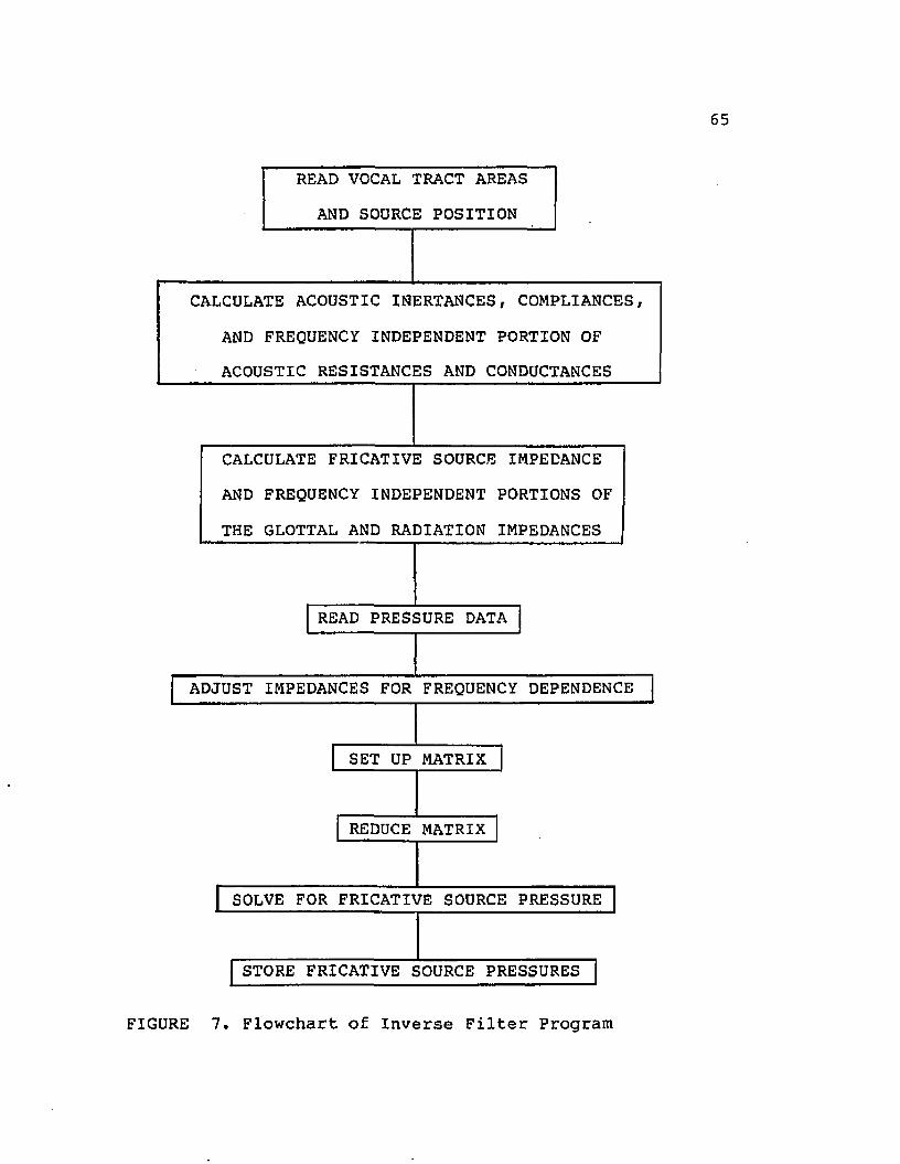
REDUCE MATRIX

SET UP MATRIX

READ PRESSURE DATA

STORE FRICATIVE SOURCE PRESSURES

SOLVE FOR FRICATIVE SOURCE PRESSURE

ADJUST IMPEDANCES FOR FREQUENCY DEPENDENCE

READ VOCAL TRACT AREASAND SOURCE POSITION

AND FREQUENCY INDEPENDENT PORTIONS OFTHE GLOTTAL AND RADIATION IMPEDANCES

CALCULATE FRICATIVE SOURCE IMPEDANCE

CALCULATE ACOUSTIC INERTANCES, COMPLIANCES

ACOUSTIC RESISTANCES AND CONDUCTANCESAND FREQUENCY INDEPENDENT PORTION OF

FIGURE 7. Flowchart of Inverse Filter Program

66

portion of the radiation resistance is calculated. Otherwise, the radiation impedance calculations are deferred. The user is then prompted to name the file containing the measured pressure data, or in the case of intensity measurements, the files containing the two measured pressure data sets.

For each frequency band of the data, the frequency independent portions of the impedances that were calculated previously in the program are combined with the frequency dependent portions. The impedances of the elements that make up the vocal tract analog are now all calculated. For the intensity data, the acoustic velocity and radiation impedance are calculated. A circuit analysis of the vocal tract analog is accomplished next.

Since the data are given in the frequency domain, a steady state frequency analysis can be made of the vocal tract analog circuit. The mesh current method was used to achieve the analysis. Simply, the mesh current method consists of assigning to each loop of the circuit a current. The assigned current represents

67

the acoustic volumetric flow between tube junctions. By summing voltages around the loops, a matrix equation is developed. The matrix equation that develops is based on the currents being unknowns and any voltage sources being known. The resulting coefficient matrix consists of a main diagonal with an off diagonal above and below. A matrix with only nonzero entries on the diagonals is often referred to as- banded. In the present study, the voltage across the radiation impedance, which simulates the measured pressure radiated from the lips, is known, and the voltage of the presure source that represents the fricative source is unknown. The known pressure across the radiation impedance is equivalent to knowing the loop current between the radiation impedance and the portion of the circuit representing the last tube section of the vocal tract. The role of this known loop current and the unknown pressure source must be reversed. The reversal of roles is accomplished by a rearrangement of the matrix equation. An optimal rearrangement results in a banded coefficient matrix with one off diagonal above the main diagonal and two below. Additionally, the diagonal above the main diagonal is zero for consecutive rows, and the second off diagonal below the main diagonal is zero for consecutive rows. The zeros

68

of the off diagonals are represented in Figure 8. Knowledge of the portion of the off diagonals that are zero and the banding of the coefficient matrix is used to minimize computations. As a result, for 512 frequency bands and approximately forty tube sections, the calculations take about 15 seconds.

Cl 0 0 0 0 0 0 0 0 0B2 C2 0 0 0 0 0 0 0 0A3 B3 C3 0 0 0 0 0 0 00 A4 B4 C4 0 0 0 0 0 00 0 A5 B5 C5 D5 0 0 0 00 0 0 A6 B6 06 D6 0 0 00 0 0 0 0 B7 C7 D7 0 00 0 0 0 0 0 B8 C8 D8 00 0 0 0 0 0 0 B9 C9 D90 0 0 0 0 0 0 0 BIO CIOFigure 8. Symbolic Matrix that Displays theSegmentation of Zeros in the Off Diagonals.

A check of the inverse filter program can be made by incorporating slight modifications to the program and analyzing the vowel "a" used in the present study. The results should produce an inverse filter function with antiresonances that correspond to the vowel formants. The modifications include the use of a high

69

resistive glottal impedance term and the use of a constant value for the pressure at any frequency. A constant value independent of frequency simulates white noise. The value of the resistance used for the glottal impedance is 200 acoustic ohms. The use of the high resistive glottal impedance transforms the vocal tract analog that the inverse filter program is based on, into the vocal tract analog that Fant used [4]. Among other uses, Fant [4] used his electrical vocal tract for the calculation of vowel resonances. The test case is run using the vocal tract area function for the vowel "a". For this vowel, Fant calculated the first three formant frequencies to be 630, 1070, and2400 Hz. The inverse filter program calculated antiresonances for the vowel "a", within the 16 Hz frequency band increments used in the calculations, at the same frequencies.

The inverse filter function is shown in Figure 9.

The matching of the formant and antiresonant frequencies indicates proper implementation of the vocal tract analog by the inverse filtering program.

Sound

Pressure

Level

(dB)

180

1704

160.-

150 --

140..

130 -.

1 2 0 -

110 - -

10080005000 6000 70004000300020001000

Frequency (Hz)Figure 9. Inverse Filter Function for Vowel "a" with High

Resistive Glottal Impedance. -j

71

Fourier Series

For the calculated fricative source spectra, 512 frequency bands of 16 Hz bandwidth are used. A Fourier series fit to the calculated spectra is performed in order to condense the necessary information needed for future use of the spectra. Since a Fourier series is employed, the source spectra are assumed periodic in the frequency domain. A formulation of the well known integral equations for the Fourier coefficients are required in discrete form. The following equations are used:

P(f) = A 3/2 + £ £ A qcos{2 7Tqf/F) + B gsin(2 77qf/F ) J (31a)q

A 0 = 2/M£p(mf) (31b)m

A q = 2/M£p(mI>cos{2 77'qm/M) (31c)mB q = 2/M£p(mI)sin{277‘qm/M) (31d)m

where P is the source pressure, A q and Bq are the Fourier coefficients, f is the frequency, F is the maximum frequency, m is the frequency band, M is the total number of frequency bands, and I is the frequency bandwidth.

4. EXPERIMENTAL MEASUREMENTS

The acquisition of fricative sound pressure spectra for the unvoiced fricatives /f/, /th/, /s/, /sh/, and /h/ is needed to compute the corresponding source spectra. Fricative sound pressure spectra that contain the important characteristics of the spectra and exclude transient characteristics are the main goal. The computations will involve the utilization of the inverse filter model based on the vocal tract analog. By applying the inverse filter model to the measured random spectra, the spectra of the random voltage source used to model the fricative source can be determined. Thus, the resulting voltage source spectra represents the fricative sound source spectra.

Experimental Procedure

The necessary measurements of the fricative sound pressure spectra were made in a semi-anechoic environment. Although the author has had no training in the production of speech for research or synthesis purposes, the necessary fricative consonants were produced by the author. The lack of training should not be a severe limitation on the credibility of the data since the author's native language is General

72

73

American.

The sound pressures were measured by placing a one-quarter inch microphone near the mouth of the speaker. Care was excercised such that the microphone was not placed in the air flow in order to eliminate the measurement of the pressure variation due to the flow. The signal was fed to a commercial Fast Fourier analyzer and the data stored on floppy disks. Storage was necessary in order to enable data manipulation at a later time. A schematic of the instrumentation system is shown in Figure 10,

FastFourierAnalyzerPreamplifier

Figure 10. Schematic of the Instrumentation Used in Making the Experimental Measurements.

74

The fricatives sounds are characterized by the presence of random noise. The use of a semi-anechoic environment did reduce background noise to an extent, but other steps were taken to reduce the background noise and its effects even further. The measurements were made as far away from the Fast Fourier analyzer as possible due to the emission of fan noise by the instrument. The microphone was placed as close as possible to the mouth of the speaker up to the point where near field effects were estimated as being significant. The fricative consonants were produced with as high an effort level as possible. A high effort level corresponds to a large volumetric flow rate. The requirement of intelligible production created part of the upper boundary on the effort level.

The need to sustain the fricative sound for a long time was also a factor in setting the upper boundary of the effort level. A lengthy sound was needed since more than one time record was used to average in the time domain. The Fast Fourier analyzer was capable of performing the necessary operations for storage of the time records and subsequent time averaging. The number of time averages used was based on the length of time that the fricative sounds could be sustained. Excluding /h/, no replenishing breaths were necessary.

75

For /h/, due to the low impedance of the vocal tract to flowr a period of time was allowed for one replenishing breath. Averaging was considered necessary due to the large variations noted by previous investigators in the spectra of fricatives. By averaging, a maximum amount of information that excluded spurious events could be acquired. In other words, the general trends evident in fricatives would be saved by averaging and the variations minimized. The resulting spectra's value is enhanced. Lastly, time averaging was utilized so that phase information could be retained. Averaging in the frequency domain is not allowed by Fast Fourier analyzers since phase information is distorted by frequency averaging. The time window for averaging was 0.0625 seconds. Two hundred ensemble averages were used.

For most of the fricative studied, the lips are not rounded and the piston radiation assumption may fail. To reduce any negative effects on the results in the event that the piston radiation assumption is grossly violated, measurements were made employing the intensity measurement technique. Measurements employing the intensity technique were made by the use of two microphones such that a finite approximation can be made for the pressure gradient. The two microphone

76

apparatus is shown in Figure 11. All other aspects o£ the measurement procedure were identical to the pressure measurements. Employing the finitedifference, the acoustic velocity can be calculated. The ratio of the average pressure for the two microphones to the calculated acoustic velocity is the impedance at the point of measurement. This impedance is used in the calculation of the vocal tract filter. A separation distance of 0.5 cm between the microphones enabled measurements valid up to 8 kHz.

y spacer j

clamp

microphones

Figure 11. Two Microphone Measurement Apparatus

v

77

Data

The results of previous measurements of fricative spectra can be used to judge the validity of the present measurements. As noted earlier, only the notion of general trends in the analysis of fricative spectra is practical. The signal to noise ratio is poor in the low frequency range due to the concentration of electrical and background noise at the low frequencies. Also, there is a lack of low frequency energy for fricative sounds.

The analysis of the data for the fricatives /f/and /th/ will be combined together due to theirsimilarity. The measured spectra for both the pressure and intensity measurements for /f/ and /th/ are given in Figures 12 through 15. For each case, the spectrum is mostly flat with the possible recognition of any peaks as broad and small. These characteristics were noted by Strevens [24] for /f/ and /th/ and by Hughes and Halle [45] for /f/. Hughes and Halle did not take spectral measurements of /th/. The data of Strevens show little energy below 2000 Hz. Whereas for Hughes and Halle's data, energy down to 150 Hz is visible.The present data shows energy down to 16 Hz. A separate measurement of the background noise and the

Sound

Pressure

Level

(dB)

65

55

45

35

25

15

5

-5 0 1000 2000 3000 4000 5000 6000 7000 8000Frequency (Hz)

Figure 12. Spectrum of the Sound Pressure for /f/ Obtainedfrom Pressure Measurement.

Sound

Pressure

Level

(dB)

40 --

1000 2000 6000 7000 80003000 4000 5000Frequency (Hz)

Figure 13. Spectrum of the Sound Pressure for /f/ Obtained byIntensity Measurement Technique. -jV£>

Sound

Pressure

Level

(dB)

70

60

50

40

30

20

10

00 1000 2000 3000 4000 5000 6000 7000 8000

Frequency (Hz)Figure 14. Spectrum of the Sound Pressure for /th/ Obtained

from Pressure Measurement.

Sound

Pressure

Level

(dB)

60

50

40

30

20

10

0

-100 1000 2000 3000 4000 5000 6000 7000 8000

Frequency (Hz)Figure 15. Spectrum of the Sound Pressure for /th/ Obtained by

Intensity Measurement Technique.

82

similarity in the spectra at the low frequencies indicates the energy present below about 1500 Hz for /f/ is background noise. For /th/, the signal extends down to 800 Hz. The above discussion indicate a poor signal to noise ratio for the frequency range below 1500 Hz for /f/ and for the frequency range below 800 Hz for /th/.

The spectra for /s/ from the pressure andintensity measurements are given in Figures 16 and 17. For the pressure measurements, a general rise in the spectrum centered at 4500 Hz is shown. For theintensity measurements, the center frequency is slightly shifted to 4000 Hz. Above and below the peak is a broad distribution of energy. The presence of energy above 4000 Hz is in agreement with previous data of Hughes and Halle [45] and Strevens [24]. However, the presence of energy below the peak is not in accordance with previous measurements. Considering the background noise measurement again, the energy present below 1500 Hz is mostly background noise, and, thus a poor signal to noise ratio is evident for frequency range. The large energy content above the 4000 Hz isnoteworthy since some communication systems have afrequency limit of 4000 Hz.

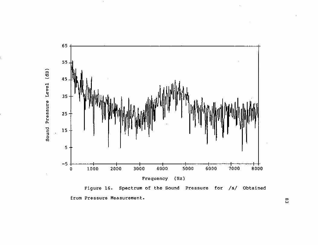
-I------- 1------- 1----------- 1------- 1----------- 1----------- 1-----------1— -0 1000 2000 3000 4000 5000 6000 7000

Frequency (Hz)Figure 16. Spectrum of the Sound Pressure for /s/

from Pressure Measurement.

8000

Obtained

Sound

Pressure

Level

(dB)

55

45

35 --

25 --

15 --

5 --

-5 --

-150 +1000 2000 3000 4000 5000 6000 7000 8000

Frequency (Hz)Figure 17. Spectrum of the Sound Pressure for /s/ Obtained by

Intensity Measurement Technique. CO

85

. The spectra for /sh/ from the pressure and intensity measurements are given in Figures 18 and 19. Peaks of energy are evident at 2500 and 5500 Hz. Again/ the energy above 4000 Hz is noteworthy due to the frequency limitations of communucation systems. As the frequency increases past the 5500 Hz peak the energy decreases, decreases in frequency past the 5500 Hz peak. Although Strevens noted more peaks in the spectra at 1000 Hz multiples for /sh/f the general trend is in agreement except for the presence of a significant amount of energy below 1000 Hz. A poor signal to noise ratio below 1000 Hz is the cause. The present data compares well with that of Hughes and Halle with the exception of the low frequency energy already noted.

The spectra for /h/ from the pressure and intensity measurements are given in Figures 20 and 21. The spectrum for /h/ is highly dependent on the vocal tract configuration. The configuration of the vocal tract may vary considerably for the production of /h/ since the turbulent flow is located at the glottis and not at some point within the vocal tract. Due to the different possible vocal tract configurations and thus filtering/ when measuring the spectra for /h/, some

Sound

Pressure

Level

(dB)

65

55

45

35

25

15

5

-5

-150 1000 2000 3000 4000 5000 6000 7000 8000

Frequency (Hz)Figure 18. Spectrum of the Sound Pressure for /sh/ Obtained

from Pressure Measurement. S

Sound

Pressure

Level

(dB)

60

50

40

30

20

10

0

-100 1000 2000 3000 4000 5000 6000 7000 8000

Frequency (Hz)Figure 19. Spectrum of the Sound Pressure for /sh/ Obtained by

Intensity Measurement Technique.

Sound

Pressure

Level

(dB)

>

-151000 2000 6000 7000 80003000 4000 5000

Frequency (Hz)Figure 20. Spectrum of the Sound Pressure for /h/ Obtained

from Pressure Measurement. 00CO

--------------1--------------1--------------j--------------1------------- 1------------- (.0 1000 2000 3000 4000 5000 6000 7000 8000

Frequency (Hz)Figure 21. Spectrum of the Sound Pressure for /h/ Obtained by

Intensity Measurement Technique.

90

known vocal tract configuration should be noted. In the present case, when the /h/ sound was produced during the measurements, the vocal tract was configured to correspond to the vowel for the "a" in father. Strevens measured the spectrum for the fricative /h/ but did not indicate any specific vocal tract configuration. The spectrum measured from the pressure measurements shows a resonant structure similar to the vowel that corresponds to the vocal tract's configuration. The first two vowel-like resonances at approximately 600 and 1000 Hz that are clearly visible in the pressure data are less defined in the intensity data. Also, a steeper decay in the spectrum is evident in the pressure measurements. The descrepancies may be due to the different positioning of the microphone for the different type measurements or the inability of the author to retain the desired vocal tract vowel configuration. The possibility of variations in the vocal tract configuration being the cause of the descrepancy was minimized by monitoring the spectra on the video display of the Fast Fourier analyzer for continuity of the spectra during the time averaging process. An adequate signal to noise ratio down to about 150 Hz seems plausible since the spectra show little similarity to the background noise above 150 Hz.

5. THE FRICATIVE SOURCE SPECTRA The following is a discussion of the fricative source spectra that are obtained by applying the inverse filter to the measured spectra. A description of the source spectra, possible explanations for the structure evident in the source spectra, and a discussion of the Fourier series approximation to the source spectra are given.

Results

Two source spectra are available for analysis from the implementation of the inverse filtering program. One spectrum is derived from the pressure measurement data, and the other, from the data obtained by the intensity measurement technique. Additionally, for each set of data, two separate source spectra corresponding to different locations of the fricative source can be calculated. Because of the poor signal to noise ratio at the low frequencies in the measured data, the portions of the source spectra at these frequencies should be disregarded.

The resulting source spectra for /f/ are shown in Figures 22, 23, 24, and 25. Figures 22 and 23correspond to the use of pressure measurements and

91

Sound

Pressu

re

Level

(dB)

110

100

90

80

70

60

50

40

30

20

100 1000 2000 3000 4000 5000 6000 7000 8000

Frequency (Hz)Figure 22. Sound Pressure Level Spectrum of the Source for /f/

Derived from Pressure Data. Source Location Downstream of theCOConstriction.

Sound

Pressure

Level

(dB)

110

1000 2000 6000 7000 80003000 4000 5000Frequency (Hz)

Figure 23. Sound Pressure Level Spectrum of the Source for /f/Derived from Pressure Data. Source Location at the Constriction. V OU)

Sound

Pressure

Level

(dB)

90

80

70

60

50

40

30

20

10

00 1000 2000 3000 4000 5000 6000 7000 8000

Frequency (Hz)Figure 24. Sound Pressure Level Spectrum of the Source for /f/

Derived from Intensity Data. Source Location Downsteam of theVO

Constriction.

Sound

Pres

sure

Level

(dB)

90

80

70

60

50

40

30

20

10

0 ------1------1------1-----1------1------1------1------H-0 1000 2000 3000 4000 5000 6000 7000 8000

Frequency (Hz)Figure 25. Sound Pressure Level Spectrum of the Source for /f/

Derived from Intensity Data. Source Location at the Constriction. en

96

Figures 24 and 25 to intensity measurements. The even numbered Figures correspond to the location of the source downstream of the constriction, and the odd numbered Figures to the location of the source within the constriction. This order of presentation will remain the same in all instances. As indicated in Figures 22 through 25, the effects of source location or measurement technique on the source spectra for /f/ is minimal. The difference between the shape of the measured pressure spectra and the calculated source spectra is also small. The flat characteristic of the measured spectra is preserved. In this case, a simple spectra for the source, such as white noise or noise that has a constant decay in amplitude as the frequency increases, seems appropriate.

The source spectra for /th/ are shown in Figures 26, 27, 28, and 29. Again,' the effect of sourcelocation or measurement technique on the source spectra is minimal. Peaks in the source spectra at 3200, 5000, 6000, 7000, and 8000 Hz are evident. No such peaks are clearly evident in the measured spectra. The lack of peaks at the same frequencies in the measured spectra is unexpected. The vocal tract should just reshape the source spectrum, not completely eliminate evidence that

Sound

Pressure'

Level

(dB)

130 120

110

100

90 80

70

60 50 40

30

200 1000 2000 3000 4000 5000 6000 7000 8000

Frequency (Hz)Figure 26. Sound Pressure Level Spectrum of the Source for

/th/ Derived from Pressure Data. Source Location Downstream of the Constriction.

Sound

Pressu

re

Level

(dB)

130

120

110

100

90

80

70 60 50

40 30

20

Frequency (Hz)Figure 27. Sound Pressure Level Spectrum of the Source for

/fch/ Derived from Pressure Data. Source Location at theConstriction.

1000 2000 4000 5000 6000 7000 8000

Sound

Pressure

Level

(dB)

85

75

65

45

25 --

15 --

40002000 3000 5000 6000 70000 1000 8000Frequency (Hz)

Figure 28. Sound Pressure Level Spectrum of the Source for /th/ Derived from Intensity Data. Source Location Downstream of the Constriction.

0 1000 2000 3000 4000 5000 6000 7000 8000Frequency (Hz)

Figure 29. Sound Pressure Level Spectrum of the Source for /th/ Derived from Intensity Data. Source Location at theConstriction.

101

a peak existed. This is true since the amplitude of the peaks in the source spectra can change with different speech levels, however the amplitude of an antiresonance of the vocal tract filter function does not change for a static vocal tract configuration. For peaks to exist in the source spectra at frequencies for which there is no peak in the measured spectra, an unlikely coincidence is needed where the speech effort level used in this study produces peaks in the source spectra that are matched in amplitude by an antiresonance in the vocal tract filter function.

Two possible explanations can be given for the existence of peaks in the source spectra without a matching peak in the measured spectra. One possibility is that the vocal tract analog is responsible for manufacturing erroneous peaks in the source spectra. If the vocal tract analog is responsible, the estimated vocal tract area for /th/ from the data available for /t/ may be the cause. Also, the assumptions of a point source or that the source impedance is only resistive may be violated. If the source impedance assumption is violated, the fact that the peaks being discussed are at high frequencies may indicate that a portion of the source impedance is inductive. Since an inductive

102

impedance increases with frequency, the effects of the inductive portion would increase with frequency. The resistive source impedance does not obey this frequency dependent effect.

The other possibility is that peaks do exist in the actual sound. In this case, either the measurement technique tended to distort the peaks or the peaks were overlooked when the data was discussed. A closer scrutinization of the measured pressure resulting from the intensity measurement technique for /th/ shows, excluding the 3200 Hz case, slight peaks at the other frequencies become visible. The presence of the slight peaks would indicate that the vocal tract damps out the resonant type phenomena in the source spectra. This damping effect is plausible. However, the explanation of the presence of peaks in the source spectra by the damping effect fails to account for the absence of the 3200 Hz peak in the measured spectrum for the intensity technique and the absence of any peaks in the measured pressure spectrum. In this case, the averaging used in the measurements may be responsible.

Peaks in the sound pressure spectra of fricatives at high frequencies have been shown before [24, 45]. However, since these high frequency peaks existed at

103

different frequencies or did not always occur/ these peaks were not considered an important aspect of the fricative sound pressure spectra. The fact that the high frequency peaks exhibit transient type behavior indicates that averaging would decrease their visibility in the measured sound pressure spectra. In this case/ a paradox exists, because the transient type behavior of the high frequency peaks is exactly what the averaging is used to minimize, yet the above discussion indicates their ir^ortance.

The source spectra for /s/ are shown in Figures 30, 31, 32, and 33. In this case, the source locationand measurement techniques show a marked effect on the source spectra. In all the spectra, two peaks at about 3500 and 4500 Hz are evident. These two peaks closely correspond to the peak in the measured spectra at approximately 4250 Hz. For the spectra corresponding to the source located downstream of the constriction, three additional peaks at 5500, 6500, and 7500 Hzappear. When the source is positioned within the constriction, the three additional peaks all shift upward in frequency by about 500 Hz. Also, the peaks at 6000 and 7000 Hz for the location of the source within the constriction have smaller amplitudes than the peaks at 5500 and 6500 Hz for the alternate source

Sound

Pressure

Level

(dB)

0 1000 2000 3000 4000 5000 6000 7000 8000Frequency (Hz)

Figure 30. Sound Pressure Level Spectrum of the Source for /s/ Derived from Pressure Data. Source Location Downsteam of the Constriction.

104

Sound

Pressu

re

Level

(dB)

115

105

95

85

75

65

55

45

350 1000 2000 3000 4000 5000 6000 7000 8000

Frequency (Hz)Figure 31. Sound Pressure Level Spectrum of the Source for /s/

Derived from Pressure Data. Source Location at the Constriction.

105

Sound

Pressure

Level

(dB)

90

80

70

60

50

40

30

20

100 1000 2000 3000 4000 5000 6000 7000 8000

Frequency (Hz)Figure 32. Sound Pressure Level Spectrum of the Source for /s/

Derived from Intensity Data. Source Location Downstream of the Constriction.

106

Sound

Pressure

Level

{dB)

90

80 -■

70

60 --

50

30 --

20 - -

101000 2000 3000 4000 5000 6000 7000 8000

Frequency (Hz)Figure 33. Sound Pressure Level Spectrum of the Source for /s/

Derived from Intensity Data. Source Location at the Constriction.

107

108

location. The amplitude of the 8000 Hz and 7500 Hz peaks are approximately the same for the two source locations. The three additional peaks, above 5000 Hz, in the source spectra are worthy of skepticism. These peaks appear to be manufactured by the vocal tract analog, since no remnants of the peaks can be found in the measured spectra. In the case of /s/, a strong case for failure of the vocal tract analog can be made. The vocal tract configuration for /s/ includes a tongue pass constriction immediately followed by a constriction due to the teeth. Two sources of sound are possible for each constriction. Only one source is used in the vocal tract analog. The source spectrum at the tongue pass constriction would be expected to be different than the source spectrum at the teeth since the two constrictions represent different turbulent inducing mechanisms. The constriction at the teeth poses an obstacle to the flow whereas a prominent obstacle is not present for the tongue pass constriction.

Alternatively, the peaks in the source spectra of /s/ may be explained by the presence of peaks in the actual sound. The effects of averaging are to distort the peaks due to their transient type behavior.

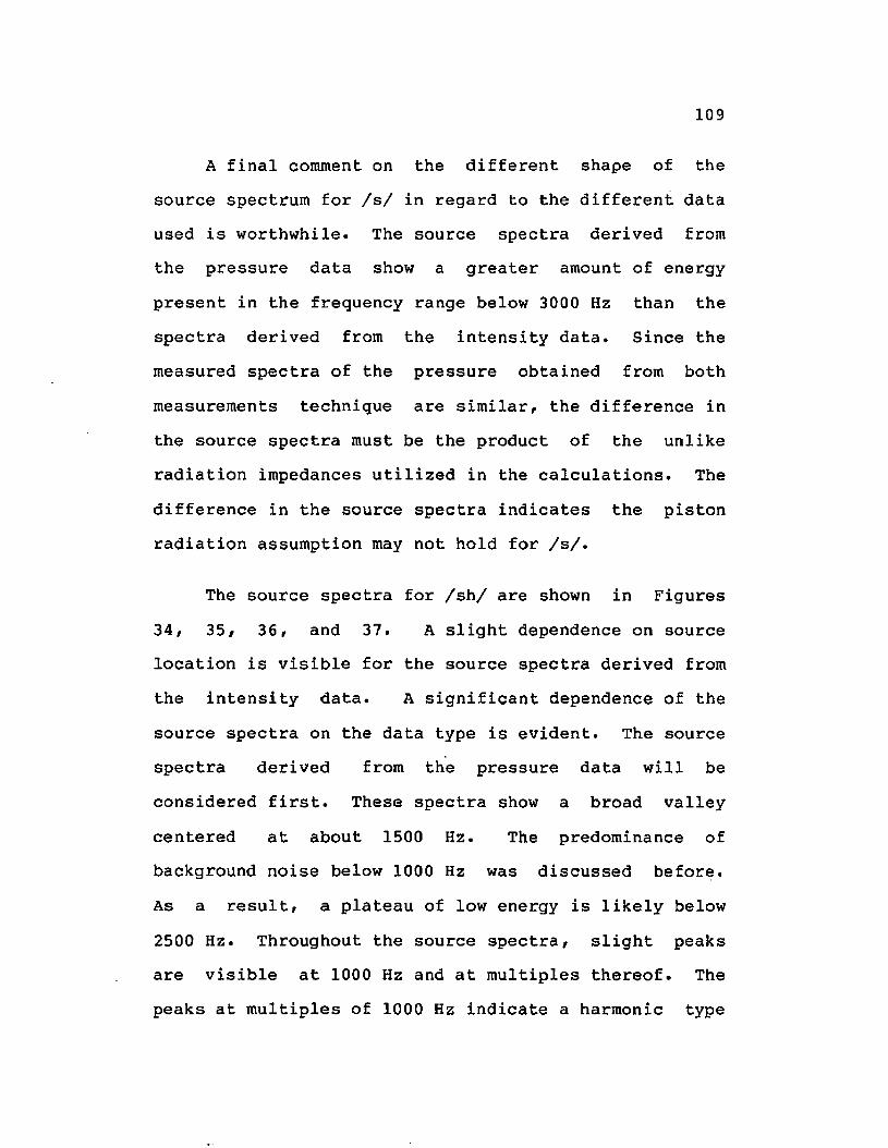
109

A final comment on the different shape of the source spectrum for /s/ in regard to the different data used is worthwhile. The source spectra derived from the pressure data show a greater amount of energy present in the frequency range below 3000 Hz than the spectra derived from the intensity data. Since the measured spectra of the pressure obtained from both measurements technique are similar, the difference in the source spectra must be the product of the unlike radiation impedances utilized in the calculations. The difference in the source spectra indicates the piston radiation assumption may not hold for /s/.

The source spectra for /sh/ are shown in Figures 34, 35, 36, and 37. A slight dependence on sourcelocation is visible for the source spectra derived from the intensity data. A significant dependence of the source spectra on the data type is evident. The source spectra derived from the pressure data will be considered first. These spectra show a broad valley centered at about 1500 Hz. The predominance of background noise below 1000 Hz was discussed before. As a result, a plateau of low energy is likely below 2500 Hz. Throughout the source spectra, slight peaks are visible at 1000 Hz and at multiples thereof. The peaks at multiples of 1000 Hz indicate a harmonic type

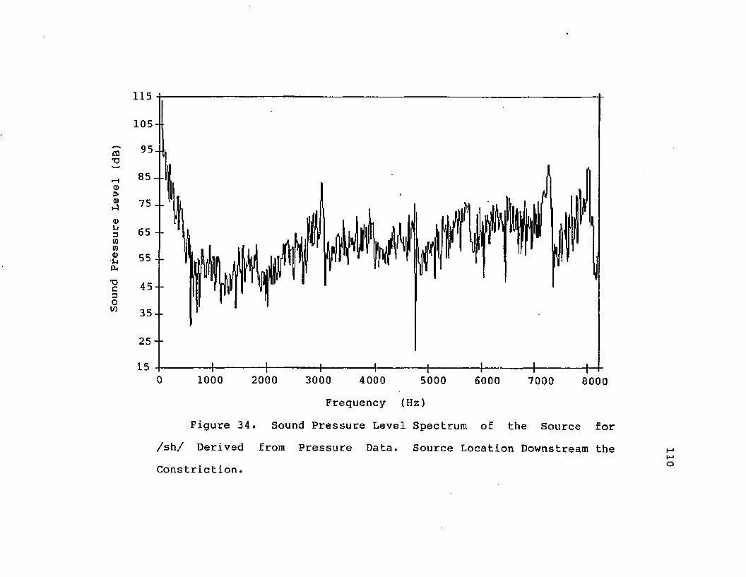
Sound

Pressure

Level

(dB)

115

105-

35--

25 —

15 -]------------- 1--------------!--------------1--------------1------------- 1------------- 1-------------1------------- ^40 1000 2000 3000 4000 5000 6000 7000 8000

Frequency (Hz)Figure 34. Sound Pressure Level Spectrum of the Source for

/sh/ Derived from Pressure Data. Source Location Downstream the Constriction.

110

Sound

Pres

sure

Level

(dB)

115

105

95

85

75

65

55

45

35

25

150 1000 2000 3000 4000 5000 6000 7000 8000

Frequency (Hz)Figure 35. Sound Pressure Level Spectrum of the Source for

/sh/ Derived from Pressure Data. Source Location at theConstriction.

Ill

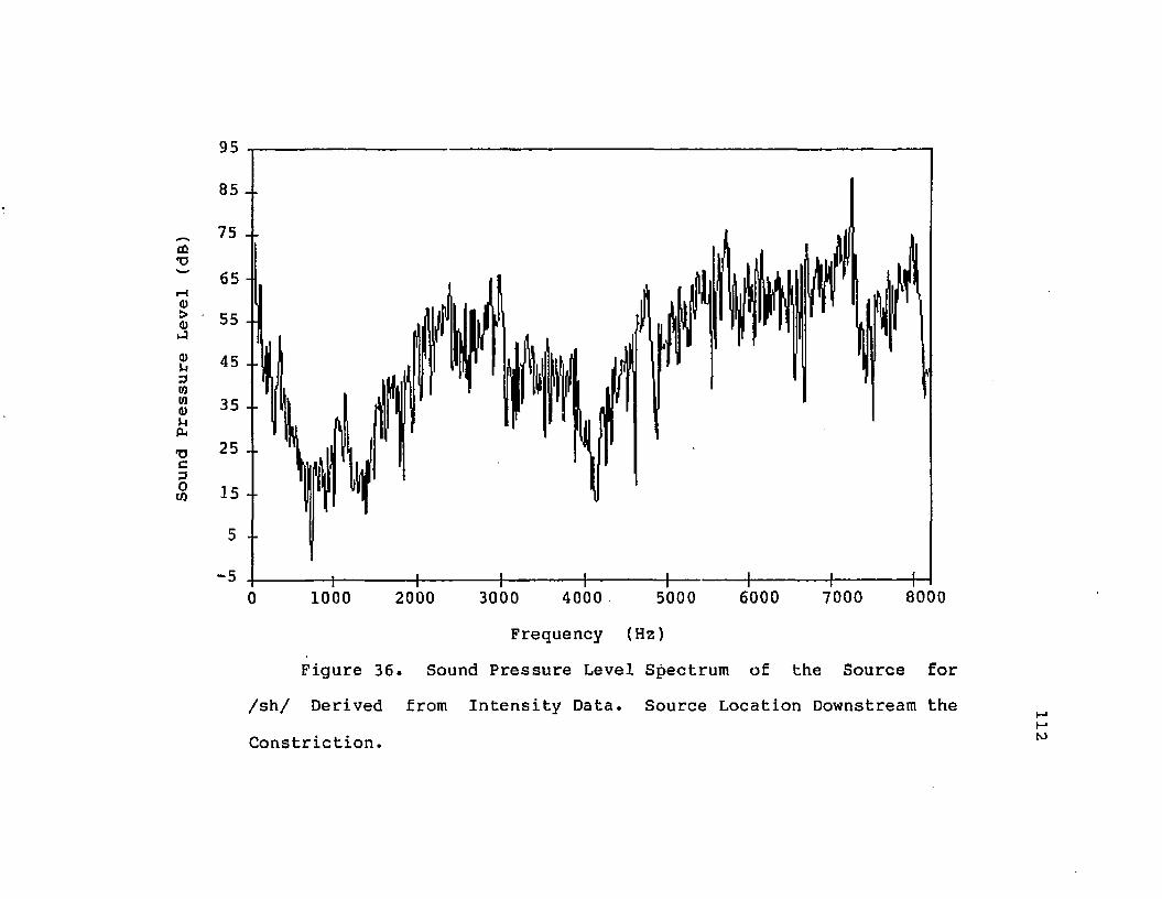
Sound

Pressure

Level

(dB)

95

85 --

75 --

65 -

45 --

35 --

25 ..

15 --

0 1000 2000 3000 4000 5000 6000 7000 8000Frequency (Hz)

Figure 36. Sound Pressure Level Spectrum of the Source for /sh/ Derived from Intensity Data. Source Location Downstream the Constriction.

112

Sound

Pres

sure

Level

(dB)

85

5 -■

"5 -I----- 1----- 1----- 1----- 1----- j----- 1----- 1----- H-0 1000 2000 3000 4000 5000 6000 7000 8000

Frequency (Hz)Figure 37. Sound Pressure Level Spectrum of the Source for

/sh/ Derived from Intensity Data. Source Location at theConstriction.

113

114

of structure. The measured pressure spectrum showed peaks at 2500 Hz and 5500 Hz. Low energy in the measured spectra was evident below 1500 Hz. A comparison of the measured pressure spectra and the calculated source spectra on the basis of the inverse filter is worthy. The effect of the inverse filter has been the removal of the peak at 2500 Hz in the measured spectra, the addition of slight peaks in the source spectra at 1000 Hz multiples except at 6000 Hz, and ageneral flattening of the measured spectra above3000Hz. Any attempt to model the source spectrum in this case should include a low frequency de-emphasis.

The dependence of the source spectra on source location for /sh/ is visible for the spectra derived from intensity data. An amplitude change is the onlyresult of the different source location with no effecton the spectral shape. The valley between the two peaks at 2500 and 5500 Hz in the pressure spectrum based on the intensity measurements is accentuated in the source spectra. A general flattening of the pressure spectrum, based on the intensity measurements, above 5500 Hz and below 7000 Hz, also seems to have occurred. Two large amplitude peaks at 7000 and ,8000 Hz appear. Remnants of these high frequency peaks may

115

be visible in the pressure spectrum from the measured data. The use of Gaussian noise to model the source spectra for /sh/ based on the spectra derived from the intensity data would be acceptable for the 500 to 4000 Hz frequency range. This type of fricative source spectrum has been used previously for speech synthesis [3] .

The significant difference in the shape of the source spectra derived for /sh/ from the two different types of data indicates a possible failure of the piston radiation assumption for this fricative.

The source spectra for /h/ are shown in Figures 38 and 39. Only one source location, downstream of the glottis, is possible in the calculation of the source spectra. The difference in the spectral shapes below 5000 Hz is largely attributed to the different spectral shapes of the pressure spectrums derived from the data. Due to the difference in the pressure spectrums based on the measured data, the piston radiation assumption could only be held partially responsible for the different source spectral shapes. The general shape of the source spectrum based on the pressure measurements will be assumed most appropriate due to the fact that the formant structure of the vowel "a" is most evident

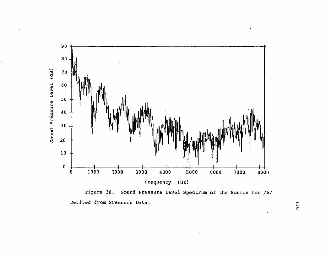
Sound

Pres

sure

Level

(dB)

90

80 -

0 1000 2000 3000 4000 5000 6000 7000 8000Frequency (Hz)

Figure 38. Sound Pressure Level Spectrum of the Source for /h/Derived from Pressure Data. 116

Sound

Pressure

Level

(dB)

70

60

50-

40--I

30--

20 - -

10 - -

-10 - -

- 2 00 1000 2000 3000 4000 5000 6000 7000 8000

Frequency (Hz)Figure 39. Sound Pressure Level Spectrum of the Source for /h/

Derived from Intensity Data.

117

118

in the pressure data. The formant type structure has been noted by a previous study [24] for the sound pressure spectrum for /h/. The source spectrum obtained from the pressure measurements shows a harmonic type structure. Large amplitude peaks are evident up to 5000 Hz. Beyond 5000 Hz, small amplitude harmonic like peaks are evident.

A final note on the piston radiation assumption used in the vocal tract analog is needed. When employing the piston radiation assumption in this study, as noted, an approximation is used for the equation of the radiation impedance. The mathematical accuracy of the equation employed decreases with frequency. When the above calculated source spectra showed a dependency on the two types of radiation impedances used the effects are most predominant at the low to mid frequency range of the study. Thus, the piston radiation assumption is violated and not the mathematical approximation.

Turbulence

On the basis of past studies of fricative production and synthesis, the structure found in the fricative source spectra are unexpected. A plausible

119

explanation for this structure would enhance the viability of the results. In order to present such anexplanation, the theory for the onset of turbulentflows will be employed. The discussion assumes that the transfer of energy from the turbulent flow into acoustic energy retains a portion of the structure ofthe flow.

As air flows through the vocal tract,perturbations in the flow will result from the irregular boundary of the vocal tract and possibly by movements of portions of the vocal tract. Under the conditions present for fricative sound production, the Reynolds number of the flow exceeds the criticalReynolds number such that the flow becomes unstable. The nature of the constriction's boundaries and the nonlinearity of the Navier-Stokes equations determine how the perturbations in the flow are amplified.Bifurcation theory predicts how the amplifications change as a flow parameter changes. Considering the Reynolds number as the flow parameter, the structure of the flow will show a harmonic type structure if the Reynolds number is below the point where chaosinitiates. Approximate Reynolds number can bedetermined for the flow rate of fricative production. For /h/, the Reynolds number at the glottis is 6300.

120

For the other fricatives, the Reynolds number at the glottis is 2700. The Reynold number at the supraglottal constriction for /f/, /th/, and /s/ is3300. For /sh/f the Reynolds number of the supraglottal constriction is 2100. In comparison to pipe flow, these Reynolds numbers are near the critical Reynolds number. The low values of the Reynolds numbers indicate that the state of chaos has not been achieved. Some harmonic structure would exist in the flow.

The source spectra for /h/ clearly exhibits a harmonic structure whereas for /sh/ a harmonic structure is less evident. The peaks in the spectra for /sh/ are at 1000 Hz multiples. The viability of the harmonic structure in the source spectra for /h/ is enhanced when the work of Hillman et al is considered. Hillman et al noted a ripple effect in their measurements of the glottal turbulent noise source. The explanation given was the failure of the reflectionless tube used in the measurements to damp out the lower formants of the vocal tract. Since the ripple effect was visible above the lower formants, the failure of the reflectionless tube is not the only reason for the ripple. The present results indicate the ripple is present in the source spectrum since the

121

inverse filtering used in the present study accentuated, instead of attenuated, the ripple present in the measured data.

The harmonic structure evident for the source spectra of /h/ may be linked to the two factors causing the onset of turbulence. The initial perturbations in the flow may be harmonic due to a slight pulsing of the air by the vocal cords. The vocal cords are abducted, pulled apart, more for /h/ than the other sounds studied. Due to the increased abduction, the vocal cords are expected to vibrate easily as the tension in the cords is released further. The harmonic pulsing of the air is amplified by the nonlinearity of the governing equations and the boundary conditions. The link between the dimensions of the glottis to both the boundary conditions and the frequency of vibration of the vocal cords may be responsible for an increase amount of amplification.

The slight harmonic structure in /sh/ may be caused by the roughness of the hard palate. The even spacing of the ridges of the hard palate may cause perturbations in the flow that are amplified as the flow becomes unstable. The resulting flow would exhibit structure related to the palate's evenly spaced

122

ridges.

Although some of the peaks in the source spectra for /th/ and /s/ may be erroneous due to the applicaion of the inverse filter, the peaks in the source spectra for /s/ at 3500 and 4500 Hz are plausible. The possibility that the peaks in the source spectra for /th/ exist is also plausible since some remnants of the peaks were seen in the measured spectra. These peaks in the source spectra for /s/ and /th/ require some explanation. The fact that the peaks in the source spectra for /th/ and /s/ seem unrelated indicates that more than one fundamental frequency may be present during the bifurcation process. As each fundamental frequency bifurcates, two additional peaks appear in the onset turbulent spectrum. Only a few bifurcations are needed for the spectrum to become complicated. Peaks in the spectrum would then seem unrelated.

The flatness of the source spectra of /f/ seems to contradict the presence of structure in the source spectra of the other fricatives studied. One explanation for the absence of structure may be that the flow for /f/ is highly turbulent which would indicate the absence of structure based on the bifurcation process. The Reynolds number and the

123

boundary conditions for the production of /f/ are similar to the other fricatives such that the liklihood that the turbulence has reached the point of chaos is diminished•

Another explanation is that structure is present but at higher frequencies than those shown. The study of sound spectra radiated by models that was conducted by Heinz [1] showed a small peak in a spectrum at 6000 Hz and a large peak at about 17000 Hz. The model used resembled the vocal tract configuration for /f/. The presence of structure at higher frequencies than used in this study is also helpful for the possible explanation of the seemingly unrelated peaks for /s/ and /th/. The fundamental frequencies for /s/ and /th/ may be significantly above the frequency ranged used in the present study such that the peaks presently visible can not be explained by a fundamental within this range.

Lastly, peaks in the source spectra for /f/ may exist, however, the peaks could be masked by a higher overall spectral energy content.

124

Model

A mathematical model for the fricative source spectra presented thus far is desired. A mathematical model would enhance the usefulness of this study of fricative source spectra for the implementation of a speech synthesizer based on the vocal tract and vocal cord analog. A mathematical model is typically judged on its ability to reduce the amount of input information necessary to obtain an output that satisfactorily characterizes the phenomenon being modelled. Parameters in the mathematical model that pertain to the actual phenomenon is a desirable feature. An initial step in the direction of constructing a mathematical model is made by representing the calculated fricative source spectra in terms of a Fourier series. The terms used are twelve sine terms, twelve cosine terms, and one constant. The number of terms utilized retain a large portion of the information of the spectra calculated. A reduction in input information from 512 parameters to twenty five is made. Retaining a large portion of the information in the calculated source spectra is necessary, since little is known about the important details of fricative sounds.

125

The twenty five coefficients used in the Fourier series representation of the spectra are given in Appendix III. Only the spectra corresponding to the location of the source downstream were considered due to the relative insensitivity of the source spectra on source location. The downstream location is picked because flows typically become turbulent during expansions of the flow. The calculated source spectra are slightly smoothed to allow for simultaneous presentation of the two versions of the source spectra. Spline functions are used in an algorithm to smooth the calculated source spectra. Minimal smoothing is employed due to the tendency of the smoothing algorithm to distort portions of the calculated source spectra.

In Figures 40 and 41, the Fourier series representation and the calculated vocal tract analog source spectra for /f/ are shown. Any representation of the source spectra would not be expected to follow the noise like characteristics. The preservation of the general shape would be the goal. The discussion of the Fourier series representation for the source spectra is based on the general shape expectation. A Fourier series representation assumes a periodic function. The existence of low energy at the higher frequencies as compared to the energy at low

Sound

Pressure

Level

(dB)

95

85 -■

75

65

55 -

45 -

35 "

250 1000 2000 3000 4000 5G00 6000 7000 8000

Frequency (Hz)Figure 40. Comparison of the Model and the Calculated Sound

Pressure Level Spectrum of the Source for /f/ Derived from Pressure Data.

126

Sound

Pressu

re

Level

{dB)

85

15 ------ 1------ 1------ 1------ 1------ h------1------ 1------ H-0 1000 2000 3000 4000 5000 6000 7000 8000

Frequency (Hz)Figure 41. Comparison of the Model and the Calculated Sound

Pressure Level Spectrum of the Source for /f/ Derived from IntensityData.

127

128

frequencies simulates a discontinuity in the function based on the periodicity assumption. A poor fit at the very beginning and end of the spectra results. This poor fit is evident' in the case of /f/. Some undulation in the Fourier series representation of the source spectra of /f/ is present. The presence of the undulation may be associated both with the source spectra and the nature of a truncated Fourier series.

Figures 42 and 43 shows the calculated vocal tract analog and the Fourier series representation of the source spectra for /th/. The most noticable difference between the two spectra is the inability of the Fourier series to match the sharp peaks of the calculatedspectra. The fact that peaks exist in the Fourierseries representation of the spectra at the same frequencies as the sharp peaks in the calculatedspectra should be sufficient in the use of the model.

The calculated and Fourier series representation of the source spectra for /s/ are shown in Figures 44 and 45. The sharp peaks in the calculated spectra are matched by the Fourier series representation to a greater degree than in the case of /th/. However, a poor match of peaks does exist at about 3800 and 4800 Hz for the source spectrum derived from pressure data

Sound

Pressure

Level

(dB)

120

110

100

90

80

70

60

50

400 1000 2000 3000 4000 5000 6000 7000 8000

Frequency (Hz)Figure 42. Comparison of the Model and the Calculated Sound

Pressure Level Spectrum of the Source for /th/ Derived from PressureData.

129

Sound

Pressure

Level

(dB)

80

70

50 -

40 --

30 --

200 20001000 3000 4000 5000 70006000 8000

Frequency (Hz)Figure 43. Comparison of the Model and the Calculated Sound

Pressure Level Spectrum of the Source for /th/ Derived fromIntensity Data.

130

Sound

Pres

sure

Level

(dB)

120

110

100

90

80

70

60

50

400 1000 2000 3000 4000 5000 6000 7000 8000

Frequency (Hz)Figure 44. Comparison of the Model and the Calculated Sound

Pressure Level Spectrum of the Source for /s/ Derived from Pressure Data.

131

Sound

Pressure

Level

(dB)

85

45

25

10000 2000 3000 4000 5000 6000 7000 8000Frequency (Hz)

Figure 45. Comparison of the Model and the Calculated SoundPressure Level Spectrum of the Source for /s/ Derived from IntensityData.

132

133

and at about 1400 Hz for the source spectrum derivedfrom the intensity data.

Figures 46 and 47 show the Fourier series representation and the calculated vocal tract analog source spectra for /sh/. The Fourier series representation does not match the sharp peaks in the calculated spectra well. The mismatch is worse for the source spectrum derived from intensity data. In either case, the poor match to the sharp peaks is in magnitude and not the result of incorrect frequencies. Exceptions to the existence of a matching peak between the two spectra are at about 1000 and 4800 Hz for the source spectrum derived from the intensity data.

The calculated and Fourier series representationof the source spectra for /h/ are shown in Figures 48and 49. The Fourier series representation matches thecalculated spectrum well with the exception of the 600 to 1200 Hz region. The mismatch in this region is believed to be a carry over of the discontinuity problem mentioned earlier. The discontinuity arise since use of the Fourier series assumes the spectra are periodic in frequency. The mismatch is believed to be minor in regard to the usefulness of the model.

Sound

Pressure

Level

(dB)

110

100

90 -

80 - f

70

60.

50 --

400 1000 2000 3000 4000 5000 6000 7000 8000

Frequency (Hz)Figure 46. Comparison of the Model and the Calculated Sound

Pressure Level Spectrum of the Source for /sh/ Derived from Pressure Data.

134

Sound

Pressure

Level

(dB)

75

65 -r

55 -

45 --

35 "

25

151000 20000 3000 4000 5000 6000 7000 8000

Frequency (Hz)Figure 47. Comparison of the Model and the Calculated Sound

Pressure Level Spectrum of the Source for /sh/ Derived fromIntensity Data.

135

Sound

Pressure

Level

(dB)

85

75

45 --

35 --

0 1000 2000 3000 4000 5000 6000 7000 8000Frequency (Hz)

Figure 48. Comparison of the Model and the Calculated SoundPressure Level Spectrum of the Source for /h/ Derived from PressureData.

136

Sound

Pressure

Level

(dB)

60

50

40

30

20

10

0

-10 0 1000 2000 3000 4000 5000 6000 7000 8000Frequency (Hz)

Figure 49. Comparison of the Model and the Calculated SoundPressure Level Spectrum of the Source for /h/ Derived from IntensityData.

137

138

The Fourier series representations given can be utilized for the spectrum of the pressure source used to simulate the fricative source in a vocal tract and vocal cord speech synthesizer. The noise like characteristics can easily be added to the model before implementation of the model in the synthesizer. A random generator could fulfill the need for the noise. Unless changes are made in the piston radiation assumption only the Fourier series representations of the source spectra derived from the pressure data can be used. This is significant for the sounds /s/ and /sh/.

6. CONCLUSIONS AND RECOMMENDATIONS

The object of this study is to determine fricative source spectra based on a vocal tract analog. Differences in the source spectra calculated by this study and those used for synthesis purposes are noted. The source spectra have an application in speech synthesizers that employ the vocal tract analog. The procedure used in this study can be used in speechanalysis work by studying variations in the sourcespectra for speech impaired subjects.

Conclusions

The use of simple spectra such as white noise or Gaussian noise for the synthesis of fricative andrelated sounds is unwise based on the results of this study. The choice of source location is not asignificant problem for speech synthesis since the source spectra calculated in this study showed little or no dependence on the position of the source. The fact that the source location is not significant in shaping the sound spectrum was also found to be true by the study of Shinobu and Shirai [61].

139

140

The dependence of the source spectra for /s/ and /sh/ indicate that modelling the radiation of sound by the lips by piston radiation is a poor assumption. The mathematical approximation used to calculate the radiation impedance is not a limiting factor.

An initial step toward modelling fricative source spectra is made. The modelling is accomplished by a Fourier series representation of the spectra. A reduction in input information of twenty to one is achieved.

Recommendations

Perception tests of fricative consonants using the source spectra calculated in this study for speech synthesis would be beneficial. The tests should also include the study of fricative consonants synthesized using the source spectra that have been previously employed in speech synthesizers.

The use of realistic physical models of the vocal tract configuration used in the production of fricatives would be the most helpful in understanding fricative source characteristics. More direct measurements of the source spectra, source distribution, and source impedance may be possible

141

without being intrusive. Dependence on the vocal tract analog to compute the source spectra would be avoided, although other filtering effects may require compensation. The physical model would allow the measurements of flow parameters and possibly lead to an understanding of the transfer of the flow energy to acoustic energy. Altering the physical model in some respects would allow the investigation of the dependence of one parameter on another. For instance, two physical models of the hard palate could be made. One with evenly spaced ridges and one that is smooth. If the use of the model with the ridges results in peaks at multiples of approximately 1000 Hz and the use of the smooth model results in a spectra with no such peaks, the peaks can be attributed to the ridges of the palate.

Some changes in the vocal tract analog may be necessary as indicated by the dependence of certain spectra on the intensity data, and thus, the piston radiation assumption. Also, the use of two sources with two different source spectra for /s/ or a distributed source for the other fricatives may be needed.

142

Relationships between the physical parameters of the human speech producing mechanism and the fricative source spectra would be beneficial. The use of the Fourier coefficients developed in this study may be useful.

BIBLIOGRAPHY

144

1. Heinz J. M., "Model Studies of the Productionof Fricative Consonants"/ Electronics LaboratoryQuarterly Progress Report/ Massachusetts Institute of Technology/ July-September, 1958/ pp. 146-149.

2. Stevens/ K. N., "Airflow and Turbulence Noise for Fricative and Stop Consonants: Static Considerations", The Journal of the Acoustical Society of America, Vol. 50, 1971, pp. 1180-1192.

3. Flanagan, J. L., "Excitation of Vocal Tract Synthesizers", The Journal of the Acoustical Society of America, Vol. 45, 1969, pp. 764-769.

4. Fant, G., Chapter 2 of Acoustic Theory ofSpeech Production, Mouton and Co., Netherlands, 1960.

5. Heinz, J. M. and Stevens, K. N., "On the Properties of Voiceless Fricative Consonants", The Journal of the Acoustical Society of America, Vol. 33, 1961, pp. 589-596.

6. Webster, A. G., "Acoustical Impedance and the Theory of Horns", Proceedings of the National of Academy of Science U. S., Vol. 5, 1919, pp. 275-282.

7. Dunn, H. K., "The Calculation of Vowel Resonances, and an Electrical Vocal Tract", The Journal of the Acoustical Society of America, Vol. 22, 1950,pp. 740-753.

8. Russell, G. 0., The Vowel, Ohio State University Press, Columbus, 1928.

9. Stevens, K. N., Kasowski, S., and Fant, C. G. M., "An Electrical Analog of the Vocal Tract", The Journal of the Acoustical Society of America, Vol. 25, 1953, pp. 734-742.

10. Fant, C. G. M., Acoustics Laboratory Quarterly Progress Report, Massachusetts Institute of Technology, July-September 1950, pp. 20.

11. Rosen, G., "Dynamic Analog Speech Synthesizer", The Journal of the Acoustical Society of America, Vol. 30, 1958, pp. 201-209.

12. Hecker, M. H. L., "Studies of Nasal Consonants with an Articulatory Speech Synthesizer", The Journal of the Acoustical Society of America, Vol.

145

34, 1962, pp. 179-188.13. Flanagan, J. L., Chapter III of Speech

Analysis Synthesis and Perception, Academic Press Inc., New York, 1965.

14. Flanagan, J. L., Ishizaka K., and Shipley K. L., "Synthesis of Speech From a Dynamic Model of the Vocal Cords and Vocal Tract", The Bell System Technical Journal, Vol. 54, 1975, pp. 485-506.

15. Flanagan, J. L. and Landgraf, L. L., "Self-Oscillating Source for Vocal Tract Synthesizers", IEEE Transactions on Audio and Electroacoustics, Vol. AU-16, 1968, pp. 57-64.

16. van den Berg, J. W., Zantema, J.T., and Doornenbal, Jr., P., "On the Air Resistance and the Bernoulli Effect of the Human Larynx", The Journal of the Acoustical Society of America, Vol. 29, 1957, pp. 626-631.

17. Mermelstein, P., "An Extension of Flanagan’s Model of Vocal-Cord Oscillations", The Journal of the Acoustical Society of America, Vol. 50, 1971, pp.1208-1210.

18. Ishizaka, >K. and Flanagan, J. L., "Synythesis of Voiced Sounds from a Two-Mass Model of the Vocal Cords", The Bell System Technical Journal, Vol. 51, 1972, pp. 1233-1268.

19. Dudgeon, D. E., "Two-Mass Model of the Vocal Cords", The Journal of the Acoustical Society of America, Vol. 48, 1970, pg. 148A.

20. Titze, I. R., "The Human Vocal Cords: AMathematical Model. Part I", Phonetica, Vol. 28,1973, pp. 129-170.

21. Titze, I. R., "The Human Vocal Cords: AMathematical Model. Part II", Phonetica, Vol. 29,1974, pp. 1-21.

22. Titze, I. R., "Normal Modes in Vocal CordTissues", The Journal of the Acoustical Society of America, Vol. 57, 1975, pp. 736-744.

146

23. Stevens, K. N., "Synthesis of Speech by Electrical Analog Devices", Journal of the Audio Engineering Society, Vol. 4, 1956, pp.2-8.

24. Strevens, S., "Spectra of Fricative Noise in Human Speech", Language and Speech, Vol. 3, 1960, pp. 32-49.

25. Hixon, T., "Turbulent Noise Sources for Speech", Folia Phonetica, Vol. 18, 1966, pp. 168-182.

26. Heinz, J. M., "Fricative Consonants", Acoustics Laboratory Quarterly Progress Report, Massachusetts Institute of Technology, October-December 1956, pp. 5-7.

27. Hillman, R. E., Oesterle, E., and Feth, L. L., "Characteristics of the Glottal Turbulent Noise Source", The Journal of the Acoustical Society of America, Vol. 74, 1983, pp. 691-694.

28. Mattingly, I. G., "Experimental Methods for Speech Synthesis by Rule", IEEE Transactions on Audio and Electroacoustics, Vol. AU-16, 1968, pp. 198-202.

29. Liljencrants, J. C. W. A., "The OVE III Speech Synthesizer", IEEE Transactions on Audio and Electroacoustics, Vol. AU-16, 1968, pp. 137-140.

30. Rabiner, L. R., "Digital Formant Synthesizerfor Speech-Synthesis Studies", The Journal of theAcoustical Society of America, Vol. 43, 1968, pp.822-828.

31. Rao, P. V. S. and Thosar, R. B., "AProgramming System for Studies in Speech Synthesis", IEEE Transactions on Acoustics, Speech, and SignalProcessing, Vol. ASSP-22, 1974, pp. 217-225.

32. Beddoes, M. B. and Chu, T. K.," DirectSample Interpolation Speech Synthesis: AnInterpolation Technique for Digital Speech Data Compression and Speech Synthesis", IEEE Transactions on Acoustics, Speech, and Signal Processing, Vol. ASSP-30, 1982, pp. 825-832.

33. Gerber, S. E., "The Intelligibility of Delta Modulated Speech", IEEE Transaction on Audio and Electroacoustics, Vol. AU-14, 1966, pp. 93-96.

147

34. Grether, C. B. and Stroh, R. W., "Subjective Evaluation of Differential Pulse-Code Modulation Using the Speech 'Goodness' Rating Scale", IEEE Transactions on Audio and Electroacoustics, Vol. AU-21, 1973, pp. 179-184.

35. Rosenthal,L. H., Rabiner, L. R., Schafer, R. W., Cummiskey, P., and Flanagan, J. L., "AMultiline Computer Voice Response System Utilizing ADPCM Coded Speech", IEEE Transactions on Acoustics, Speech, and Signal Processing, Vol. ASSP-22, 1974, pp. 339-352.

36. Rabiner, L. R. and Schafer, R. W., "Digital Techniques for Computer Voice Response: Implementations and Applications", Proceedings of the IEEE, Vol. 64, 1976, pp. 416-433.

37. Schafer, R. W. and Rabiner, L. R., "Digital Representations of Speech Signals", Proceedings of the IEEE, Vol. 63, 1975, pp. 662-677.

38. Bayless, J. W. and Campanella, S. J., "ASurvey of Speech Digitization Techniques", Kentucky University, Office of Research for Engineering Services, Bulletin K, 1972, pp. 72-84.

39. Flanagan, J. L., Schroeder, M. R., Atal, B.S., Crochiere, R. E., Jayant, N. S., and Tribolet, J.M., "Speech Coding", IEEE Transactions on Communications, Vol. COM-27, 1979, pp. 710-737.

40. Atal, B. S. and Hanauer, S. L., "Speech Analysis and Synthesis by Linear Prediction of the Speech Wave", The Journal of the Acoustical Society of America, Vol. 50, 1971, pp. 637-655.

41. Atal, B. S. and Schroeder, M.R., "Predictive Coding of Speech Signals", IEEE Weiscon Technical Papers, Vol.12, Session 8, Part 3, pp.1-7.

42. Markel, J. D. and Gray, Jr., A. H., "A Linear Prediction Vocoder Simulation Based upon the Autocorrelation Method, IEEE Transactions on Acoustics, Speech, and Signal Processing, Vol. ASSP-22, 1974, pp. 124-134.

43. Makhoul, J., "Linear Prediction: A Tutorial Review", Proceedings of the IEEE, Vol.63, 1975, pp. 561-580.

148

44. Haggard/ M. P. and Mattingly/ I. G. , "A Simple Program for Synthesizing British English", IEEE Transactions on Audio and Electroacoustics/ Vol. AU-16, 1968, pp. 95-99.

45. Hughes, G. W. and Halle, M., "Spectral Properties of Fricative Consonants", The Journal of the Acoustical Society of America, Vol. 28, 1956, pp. 303-310.

46. Monin, A. S. and Yaglom, A. M., Introduction from Statistical Fluid Mechanics I, The MIT Press, Cambridge, Massachusetts, 1971.

47. Monin, A. S. and Yaglom, A. M., From Chapter 7, Section 16 of Statistical Fluid Mechanics II, The MIT Press, Cambridge, Massachusetts, 1975.

48. Bradshaw, P., Chapter 1 of Turbulence, Springer-Verlag, New York, 1978.

49. Feigenbaum, M. J., "QuantitativeUniversality for a Class of Nonlinear Transformations", Journal of Statistical Physics, Vol. 19, 1978, pp.25-52.

50. Feigenbaum, M. J., "The Onset Spectrum of Turbulence", Physics Letters A, Vol. 74, pp. 375-378.

51. Townsend, A. A., The Structure of Turbulent Shear Flows, Cambridge University Press, 1956.

52. Grant, H. L., "The Large Eddies of Turbulent Motion", Journal of Fluid Mechanics, Vol. 4, 1958.

53. Davies, P. O. A. L., "Turbulence Structure in Free Shear Layers", AIAA Journal, Vol. 4, 1966.

54. Crow, S. C. and Champagne, F.H., "Orderly Structure in Jet Turbulence", Journal of Fluid Mechanics, Vol. 48, Pt. 3, 1971.

55. Bradshaw, P., Fevis D. H., and Johnson, R. J., "Turbulence in Noise Producing Region of Circular Jets", Journal of Fluid Mechanics, Vol. 19, 1964.

56. Ko, N. W. M., and Davies, P. O. A. L., "The Near Field Within the Potential Core of Subsonic Cold Jets", Journal of Fluid Mechanics, Vol. 50, 1971.

149

57. Mermelstein, P., "Articulatory Model for the Study of Speech Production", The Journal of the Acoustical Society of America, Vol. 53, 1973, pp. 1070-1082.

58. Coker, C. H., "A Model of Articulatory Dynamics and Control", Proceedings of the IEEE, Vol. 64, 1976, pp. 452-460.

59. Coker, C. H., Umeda, N., and Browman, C. P., "Automatic Synthesis from Ordinary English Text", IEEE Transactions on Audio and Electroacoustics, Vol. AU-21, 9173, pp. 293-298.

60. Flanagan, J. L. and Ishizaka, K. , "Automatic Generation of Voiceless Excitation in a Vocal Cord-Vocal Tract Speech Synthesizer", IEEE Transactions on Acoustics, Speech, and Signal Processing, Vol. ASSP-24, 1976, pp. 163-170.

61. Shinobu, M. and Shirai, K., "Estimation of the Vocal Tract Shape Producing Fricative Consonants", Journal Acoustical Society Japan, Vol.5, 1984, pp. 51-58.

APPENDICES

APPENDIX I Vocal Tract Areas

Table 1. Vocal Tract Areas for /f/.

Areacm2

Endpoint Position Along Vocal Tract

cm2.0 0.51.75 0.90.1 1.32.25 1.65.2 1.86.9 2.07.85 2.58.0 3.08.1 3.58.2 4.08.3 4.58.4 5.08.4 5.58.35 6.08.2 6.57.9 7.07.3 7.56.7 8.05.4 8.53.9 8.751.8 9.01.6 9.252.8 9.53.0 10.02.4 10.52.05 11.01.95 11.52.05 12.02.3 12.52.8 13.03.3 13.54.1 14.04.9 14.55.9 15.07.0 15.57.75 16.02.5 16.52.4 17.02.5 17.52.85 18.02.95 18.4

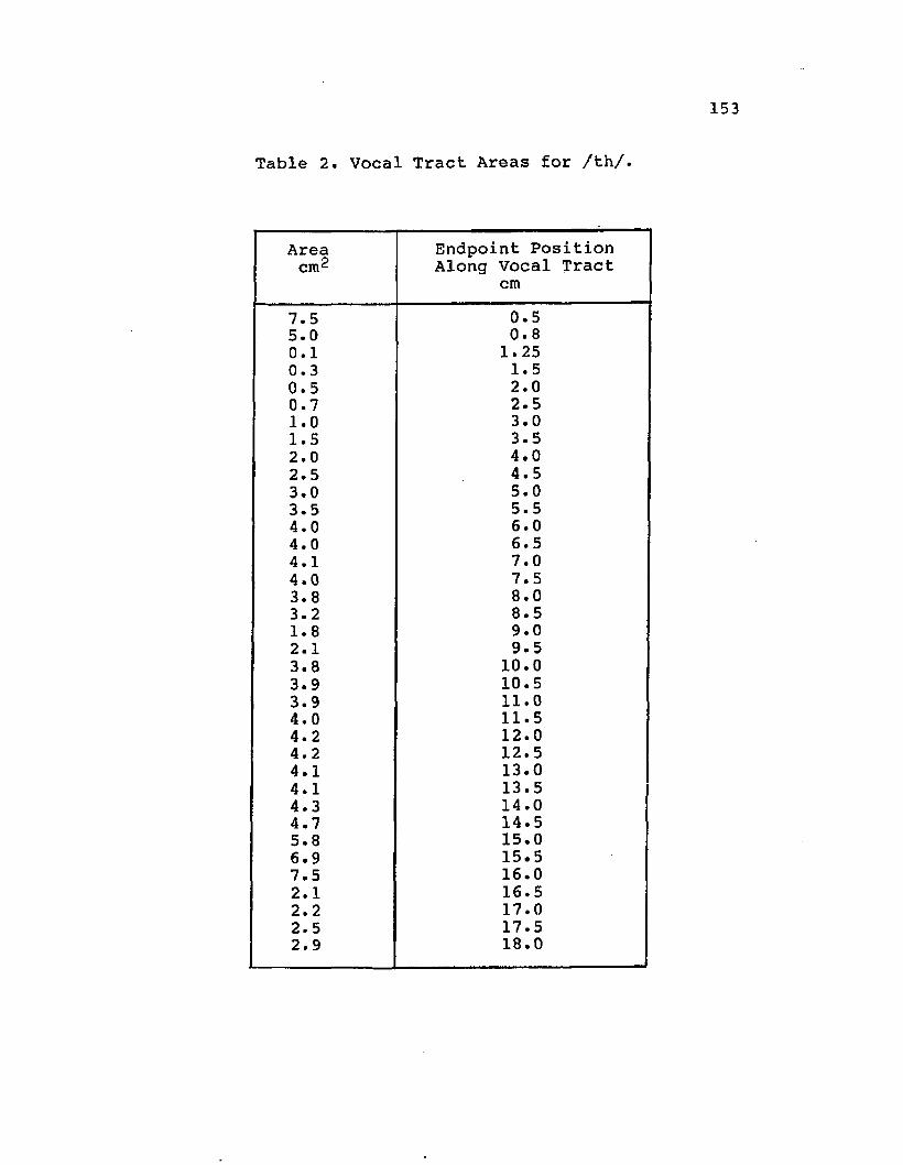
Table 2. Vocal Tract Areas for /th/.

Area cm^

Endpoint Position Along Vocal Tract

cm7.5 0.55.0 0.80.1 1.250.3 1.50.5 2.00.7 2.51.0 3.01.5 3.52.0 4.02.5 4.53.0 5.03.5 5.54.0 6.04.0 6.54.1 7.04.0 7.53.8 8.03.2 8.51.8 9.02.1 9.53.8 10.03.9 10.53.9 11.04.0 11.54.2 12.04.2 12.54.1 13.04.1 13.54.3 14.04.7 14.55.8 15.06.9 15.57.5 16.02.1 16.52.2 17.02.5 17.52.9 18.0

Table 3. Vocal Tract Areas for /s/.

Areacm2Endpoint Position Along Vocal Tract

cm6.4 0.55.5 0.72.1 0.90.25 1.30.1 1.70.1 2.10.1 2.50.4 3.00.85 3.51.75 4.02.7 4.53.4 5.03.8 5.53.8 6.03.9 6.53.75 7.03.8 7.53.85 8.03.55 8.52.9 8.72.35 9.02.9 9.24.0 9.54.95 10.04.65 10.56.2 11.06.8 11.57.2 12.07.6 12.57.95 13.08.2 13.58.5 14.08.75 14.59.2 15.03.5 15.53.2 16.03.1 16.53.0 17.02.9 17.5

Table 4. Vocal Tract Areas for /sh/.

Areacm2

Endpoint Position Along Vocal Tract

cm8.0 0.57.0 1.04.75 1.21.75 1.68.9 2.09.0 2.58.9 3.00.75 3.20.25 3.60.75 4.01.9 4.53.5 5.04.5 5.54.25 6.04.15 6.54.4 7.04.5 7.54.0 8.03.8 8.52.8 9.01.3 9.52.25 10.02.1 10.51.7 11.01.4 11.51.6 12.01.9 12. 52.5 13.03.25 13.53.8 14.04.75 14.55.6 15.06.0 15.56.5 16.06.8 16.52.3 17.02.5 17.52.9 18.03.0 18.5

Table 5. Vocal Tract Areas for /h/.

AreacinEndpoint Position Along Vocal Tract

cm5.0 0.55.0 1.05.0 1.56.5 2.08.0 2.58.0 3.08.0 3.58.0 4.08.0 4.58.0 5.08.0 5.58.0 6.06.5 6.55.0 7.04.0 7.53.2 8.01.6 8.52.6 9.02.6 9.52.0 10.01.6 10.51.3 11.01.0 11.50.65 12.00.65 12.50.65 13.01.0 13.51.6 14.02.6 14.54.0 15.01.0 15.51.3 16.01.6 16.52.6 17.0

APPENDIX II Computer Program Listing

158

BYTE ID(80),NAME1(30),NAME2(30)REAL LENGTH(60),MU,LAMBDA,LA(45)DIMENSION AREA{60),R{60),G(60),CA(60),S(45) COMPLEX A(60),B(60),C(60),D(60),X(60)COMPLEX ZRl,ZR,ZA1,ZA2, ZB1,ZB2,E1,E2,DAT(513),ZG DATA LUN1,LUN2,LUN3/10,11,13/1=0RJNK=0.0TYPE * ,'$ENTER VOCAL TRACT AREA FILENAME:'ACCEPT 10,LEN,NAME1

10 FORMAT (Q,30A1)CALL ASSIGN (LUN1,NAME1,LEN)

1 1=1+1READ (LUN1,15,END=20)AREA(I),POSITN,ISOR LENGTH(I)=POSITN-RJNK RJNK=POSITN GOTO 1

20 CONTINUECALL CLOSE(LUNl)

15 FORMAT (2F6.3,I3)NVTS=IRHO=l.14E-3CSUB0=3•5E4MU=1.86E-4LAMBDA=0.055E-3CSUBP=0•24PI=3.14159265DO 25 I=1,NVTS-1S (I)= 2 * SQRT(AREA(I)*PI)CA(I)=AREA(I)/RHO/CSUBO * * 2 G( I )=0.4*S(I)/RHO/CSUBO**2*+ SQRT{LAMBDA/2/CSUBP/RHO)LA(I)=RHO/AREA{I )R(I)=S(I )/AREA(I )**2*SQRT{RHO*MU/2)

25 CONTINUETYPE *,1$ENTER THE FILENAME FROM WHICH

+ THE DATA WILL BE READ:'ACCEPT 10,LEN,NAME1CALL ASSIGN(LUN3,NAME1,LEN)TYPE *,'$ENTER THE FILENAME WHERE THE

+ RESULTS WILL BE STORED:'ACCEPT 10,LEN,NAME2CALL ASSIGN(LUN2,NAME2,LEN)DO 40 1=1,13 READ (LUN3,45)ID

40 CONTINUE 45 FORMAT (80A1)

DO 50 1=1,512,3READ (LUN3,55){DAT{K),K=I,1+2)

50 CONTINUE

159

55 FORMAT (6E13.5)F=16.0DO 86 1=1/NVTS D(I)=(0.0,0.0)B(I)=(0.0,0.0)A(I)=(0.0,0.0)

86 CONTINUE Rl=SQRT(AREA(1 )/PI)AREA(NVTS)=0.15 U=300IF(ISOR.LT.15)GOTO 87 AREA(NVTS)=0.3 U=1000

87 WIDTH=AREA(NVTS)/I.8 DEPTH=0.3Z G 0=12 *MU * DE PTH/AREA(NVTS)/WIDTH * * 2+

+ 0.9*RHO*U/2/AREA(NVTS)**2ZGl=RHO*DEPTH/AREA(NVTS)ZSOR=RHO*U/2/AREA(ISOR)**2ZR1=CMPLX((R1/CSUB0)**2/2,8*Rl/CSUB0/3/PI)*

+ RHO*CSUBO/PI/R1**2 DO 60 J=1,512 W=2*PI*FZG=CMPLX(ZG0,W*ZG1)ROOTW=SQRT(W)RA=ROOTW* R (1)GA=ROOTW*G(1)ZA1=CMPLX(RA,W*LA(1))*LENGTH(1)/2. 0 ZB1=1.0/CMPLX(GA,W* CA(1))/LENGTH(1) ZR=CMPLX(W**2*REAL(ZRl),W*AIMAG(ZRl))C(1)=-ZB1El=-(ZR+ZAl+ZBl)*DAT(J )/ZR RA=ROOTW*R(2)GA=ROOTW*G(2)ZA2=CMPLX(RA,W*LA(2))*LENGTH(2)/2.0ZB2=1.0/CMPLX(GA,W*CA(2))/LENGTH(2)B(2)=ZA1+ZA2+ZB1+ZB2C ( 2 ) =-ZB2E2=ZB1*DAT(J)/ZRDO 65 1=3,NVTS-1RA=ROOTW*R(I )GA=ROOTW*G(I)ZA1=ZA2ZB1=ZB2ZA2=CMPLX(RA,W*LA(I))*LENGTH(I)/2.0 ZB2=1.0/CMPLX(GA,W*CA(I))/LENGTH(I)IF(I.GE.ISOR) GOTO 70 A( I )=-ZBlB(I)=ZAl+ZA2+ZBl+ZB2 C( I)=-ZB2

160

GOTO 65 70 IF(I.GT.ISOR) GOTO 75

A{I)=-ZBlB(I)=ZAl+ZA2+ZBl+ZB2+ZSOR C{I)=-1 D(I)=-ZB2 GOTO 65

75 IF(I.GT.ISOR+1) GOTO 80A( I)=-ZBlC(I)=ZAl+ZA2+ZBl+ZB2 D(I)=-ZB2 GOTO 65

80 B {I)--ZB1C(I)=ZA1+ZA2+ZB1+ZB2 D(I)=-ZB2

65 CONTINUEB(NVTS)=-ZB2C(NVTS)=ZB2+ZA2+ZGIF{ISOR.NE.NVTS) GOTO 89A (NVTS)=-ZB2B(NVTS)=ZA2+ZB2+ZGC (NVTS)—-1GOTO 91

89 DO 90 1=1fNVTS-ISOR K=NVTS-I+1 A(K)=A(K)/C(K)B(K)=B(K)/C(K)B(K-1)=B(K-1)-D(K-1)*A(K)C (K-l)=C(K—1)-D{K-l)*B(K )

90 CONTINUE91 X(1)=E1/C(1)

X(2)=(E2-B(2)*X{1))/C(2)DO 95 1=3fISORX(I)=-(B(I)*X(1-1)+A(I)*X{1-2))/C(I)

95 CONTINUEDAT(J )=X(ISOR)F=F+16

60 CONTINUEDO 100 1=1r512 ,3WRITE (LUN2,55)(DAT(K),K=I,I+2)

100 CONTINUECALL CLOSE(LUN3)CALL CLOSE(LUN2)STOPEND

APPENDIX III Fourier Series Coefficients

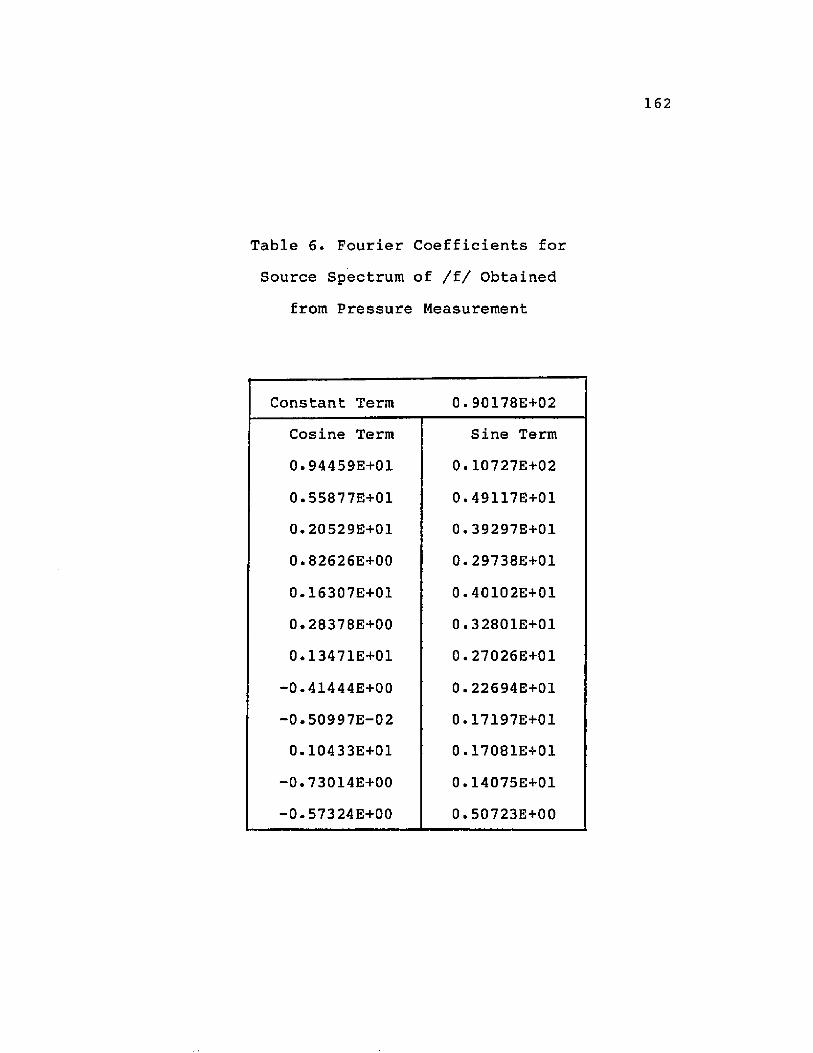
Table 6. Fourier Coefficients forSource Spectrum of /f/ Obtained

from Pressure Measurement

Constant Term 0.90178E+02Cosine Term Sine Term0.94459E+01 0.10727E+020.55877E+01 0.49117E+010.20529E+01 0.39297E+010 • 82626E+00 0.29738E+010.16307E+01 0•40102E+010.28378E+00 0.32801E+010.13471E+01 0•27026E+01

-0.41444E+00 0.22694E+01-0.50997E-02 0.17197E+010.10433E+01 0.17081E+01

-0.73014E+00 0.14075E+01-0.57324E+00 0.50723E+00

Table 7. Fourier Coefficients forSource Spectrum of /f/ Obtained

from Intensity Measurement Technique

Constant Term 0.67827E+02Cosine Term Sine Term0.10124E+02 0.13626E+010.39730E+01 0.26312E+010.19724E+01 0.26730E+010.21300E+01 0.32981E+010.26100E+01 0.22885E+010.73892E+00 0.26434E+010.23466E+00 0.25231E+010.67056E+00 0.22923E+01

-0.30710E+00 0.24117E+010.54293E+00 0•94795E+000.66939E-01 0.14263E+010.23821E+00 0.14321E+01

Table 8. Fourier Coefficients forSource Spectrum of /th/ Obtained

from Pressure Measurement

Constant Term 0.13300E+03Cosine Term Sine Term0.81714E+01 0.87839E+010.12349E+01 0.29513E+010.14475E+01 0.29593E+01

“0•15588E+01 0•38388E+010.15324E+01 0.37774E+010.77431E+00 0.22913E+010.27824E+01 0.23950E+000.13378E+01 0.12218E+01

-0.18068E+01 0.29487E+000.16678E+01 0.15075E+01

-0.22457E+01 -0.20531E+01-0.23909E+01 0.95436E+00

Table 9. Fourier Coefficients forSource Spectrum of /th/ Obtained

from Intensity Measurement Technique

Constant Term 0. 93470E+02Cosine Term Sine Term0.63374E+01 -0. 42552E+010.32500E+01 0.18298E+000.23403E+01 0.46527E+00

-0.24513E+01 0.22286E+010.22367E+01 0.25445E+010•32907E+00 0.21130E+010.35840E+01 0.57378E+000.14357E+01 -0.33680E+00

-0.24944E+01 -0.20862E+000.18556E+01 0.14161E+01

-0.30854E+01 -0.14637E+01-0.20717E+01 0.71936E+00

Table 10. Fourier Coefficients forSource Spectrum of /s/ Obtained

from Pressure Measurement

Constant Term 0.13481E+03Cosine Term Sine Term0.29626E+01 -0.16731E+010.36719E+01 0.60122E+010.10704E+01 0.15625E+010.10618E+01 0.89252E+00

-0.23795E+00 0.93047E+000.37972E+00 0 * 65711E+00

-0•63300E+00 0.64745E+00-0.27824E+01 0.33326E+010.27614E+01 0.53750E+010.23501E+01 0.61070E+000.45193E+00 -0.77013E+00

-0.81032E+00 0.55070E+00

Table 11. Fourier Coefficients forSource Spectrum of /s/ Obtained

from Intensity Measurement Technique

Constant Term 0.10587E+03Cosine Term Sine Term

-0•78583E+01 -0.15983E+020.45978E+01 -0.39283E+010.14988E+01 -0.13625E+010.25687E+01 -0.43399E+010.22578E+00 -0.86895E+000.78745E+00 “0.10929E+01

“0.48524E+00 -0.49822E+00-0•21638E+01 0.33015E+010.26895E+01 0.44 235E+010.23348E+01 -0.22538E+000.16020E+01 -0.14829E+01

-0.31749E+00 -0.38734E+00

Table 12. Fourier Coefficients forSource Spectrum of /sh/ Obtained

from Pressure Measurement

Constant Term 0.12365E+03Cosine Term Sine Term0.22030E+01 -0.69015E+010. 29321E+01 -0.45188E+010. 39102E+01 0.11789E+010.21260E+01 0.51207E+000.12255E+01 0.62433E+000•29977E+01 0.16193E+010.10767E+01 0.10372E+010.42511E-01 0•63607E+000.19638E+01 0.40178E+00

-0.83461E+00 -0•68594E+00-0.57154E+00 0.12318E+01-0.23141E+01 0.18103E+01

Table 13. Fourier Coefficients forSource Spectrum of /sh/ Obtained

from Intensity Measurement Technique

Constant Term 0.10587E+03Cosine Term Sine Term

-0.78583E+01 -0•15983E+020.45978E+01 -0.39283E+010.14988E+01 -0.13625E+010.25687E+01 -0.43399E+010.22578E+00 -0.86895E+000.78745E+00 -0.10929E+01

-0.48524E+00 -0.49822E+00-0.21638E+01 0.33015E+010.26895E+01 0.44235E+010.23348E+01 -0.22538E+000.16020E+01 -0.14829E+01

-0.31749E+00 -0.38734E+00

Table 14. Fourier Coefficients forSource Spectrum of /h/ Obtained

from Pressure Measurement

Constant Term 0 * 67430E+02Cosine Term Sine Term0.10209E+02 0.11672E+020«38607E+01 0.31537E+010.24416E+00 0.42360E+010.41908E+00 0.39980E+01

-0.28280E+00 0.10670E+010.59257E+00 0.32723E+01

-0.13253E+00 -0.30394E+00-0.61011E-01 0.45255E+01-0.29595E+01 0.33102E+010.23618E+00 -0.69898E+000.10652E+01 0.77650E+000.10883E+01 0.11339E+01

Table 15. Fourier Coefficients forSource Spectrum of /h/ Obtained

from Intensity Measurement Technique

Constant Term 0.44590E+02Cosine Term Sine Term0.76121E+01 0.82276E+010.52872E+01 -0.13181E+01

-0.95339E+00 0.55212E+010 * 76912E+00 0.22074E+01

-0.24529E+01 0.46500E+000 *14706E+01 0.10773E+01

-0.23009E+01 -0•10837E+00-0.10237E+01 0.36662E+010.16520E+01 0.25656E+01

-0.46359E-01 0.72915E+000.42693E+00 0.75665E+000.42774E+00 0.14488E+01

VITA

The author, Lawrence Edward Zagar, was born February 5, 1959 in Bronxville, New York. He is theson of Mr. and Mrs. W. T. Zagar. The author was a graduate of St. George Elementary School and Catholic High School/ both located in Baton Rouge, Louisiana. In 1977, he entered Louisiana State University and received his B. S. degree in Mechanical Engineering in May 1981. In September of 1981, he entered the graduate school at Louisiana State University and received his M. S. in Mechanical Engineering in the May of 1983.

The author married Jane Valiquette in August 1982. In December 1985, the author became the proud father of Hannah Christine Zagar.

The author is currently enrolled in Louisiana State University pursuing a Doctor of Philosophy degree in Mechanical Engineering.

172

DOCTORAL EXAMINATION AND DISSERTATION REPORT

Candidate: Lawrence E. Zagar

Major Field: M echanical E n g in eer in g

Title of Dissertation; The F r ic a t iv e Sound Source Spectrum D erived from a V ocalT ract Analog

Approved:

and Chairman

UI--Dean of^theGradu e School

EXAMINING COMMITTEE:

l-p1. C^cXJLr^r-

/! VUA(iH-

Date of Examination:

April 25, 1986