Lecture 2 - 1, July 21, 2008

NBER Summer Institute Minicourse – What’s New in Econometrics: Time Series

Lecture 2:

July 14, 2008

The Functional Central Limit Theorem and

Testing for Time Varying Parameters

Lecture 2 - 2, July 21, 2008

Outline

1. FCLT

2. Overview of TVP topics (Models, Testing, Estimation)

3. Testing problems

4. Tests

Lecture 2 - 3, July 21, 2008

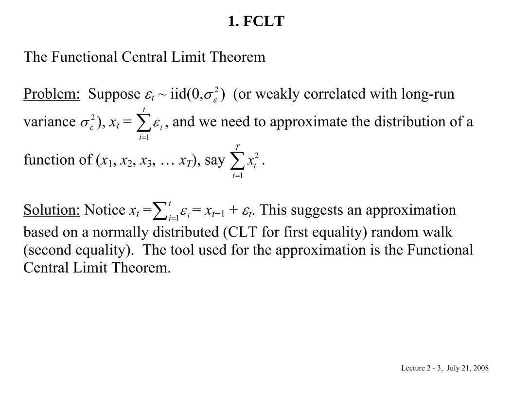
1. FCLT The Functional Central Limit Theorem Problem: Suppose εt ~ iid(0, 2

εσ ) (or weakly correlated with long-run

variance 2εσ ), xt =

1

t

iiε

=∑ , and we need to approximate the distribution of a

function of (x1, x2, x3, … xT), say 2

1

T

tt

x=∑ .

Solution: Notice xt = 1

tiiε

=∑ = xt−1 + εt. This suggests an approximation based on a normally distributed (CLT for first equality) random walk (second equality). The tool used for the approximation is the Functional Central Limit Theorem.

Lecture 2 - 4, July 21, 2008

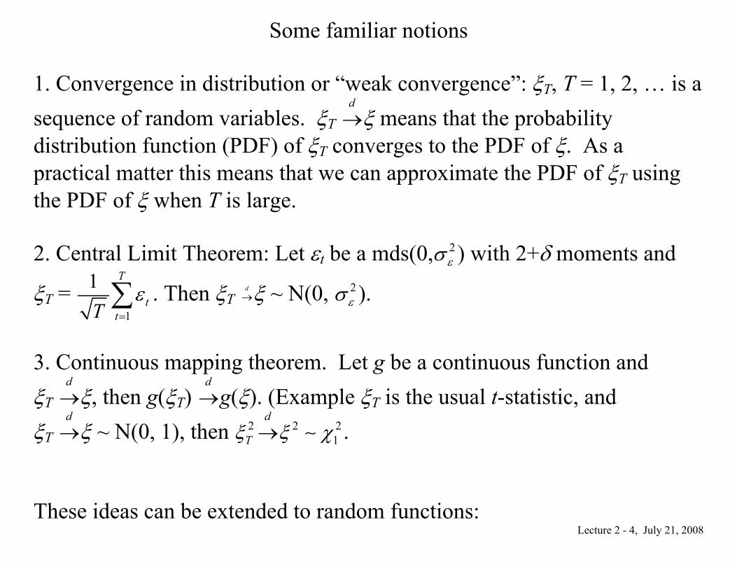
Some familiar notions 1. Convergence in distribution or “weak convergence”: ξT, T = 1, 2, … is a sequence of random variables. ξT

d→ξ means that the probability

distribution function (PDF) of ξT converges to the PDF of ξ. As a practical matter this means that we can approximate the PDF of ξT using the PDF of ξ when T is large. 2. Central Limit Theorem: Let εt be a mds(0, 2

εσ ) with 2+δ moments and

ξT = 1

1 T

ttTε

=∑ . Then ξT d

→ξ ~ N(0, 2εσ ).

3. Continuous mapping theorem. Let g be a continuous function and ξT

d→ξ, then g(ξT)

d→g(ξ). (Example ξT is the usual t-statistic, and

ξT d→ξ ~ N(0, 1), then 2 2 2

1

d

Tξ ξ χ→ ∼ . These ideas can be extended to random functions:

Lecture 2 - 5, July 21, 2008

A Random Function: The Wiener Process, a continuous-time stochastic process sometimes called Standard Brownian Motion that will play the role of a “standard normal” in the relevant function space.

Denote the process by W(s) defined on s [0,1] with the following properties 1. W(0) = 0 2. For any dates 0 ≤ t1 < t2 < … < tk ≤ 1, W(t2)−W(t1), W(t3)−W(t4), … , W(tk)−W(tk−1) are independent normally distributed random variables with W(ti)−W(ti−1) ~ N(0, ti−ti−1). 3. Realizations of W(s) are continuous w.p. 1. From (1) and (2), note that W(1) ~ N(0,1).

Lecture 2 - 6, July 21, 2008

Another Random Function: Suppose εt ~ iidN(0,1), t = 1, … , T, and let ξT(s) denote the function that linearly interpolates between the points

ξT(t/T) = 1

1 t

iiTε

=∑ .

Can we use W to approximate the probability law of ξT(s) if T is large? More generally, we want to know whether the probability distibution of a random function can be well approximated by the PDF of another (perhaps simpler, maybe Gaussian) function when T is large. Formally, we want to study weak convergence on function spaces. Useful References: Hall and Heyde (1980), Davidson (1994), Andrews (1994)

Lecture 2 - 7, July 21, 2008

Suppose we limit our attention to continuous functions on s [0,1] (the space of such functions is denoted C[0,1]), and we define the distance between two functions, say x and y as d(x,y) = sup0 ≤ s ≤ 1 |x(s) – y(s)|. Three key theorems (Hall and Heyde (1980) and Davidson (1994, part VI):

Lecture 2 - 8, July 21, 2008

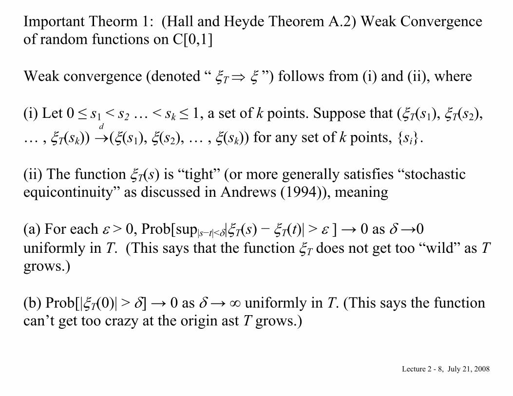
Important Theorm 1: (Hall and Heyde Theorem A.2) Weak Convergence of random functions on C[0,1] Weak convergence (denoted “ ξT ⇒ ξ ”) follows from (i) and (ii), where (i) Let 0 ≤ s1 < s2 … < sk ≤ 1, a set of k points. Suppose that (ξT(s1), ξT(s2), … , ξT(sk))

d→(ξ(s1), ξ(s2), … , ξ(sk)) for any set of k points, {si}.

(ii) The function ξT(s) is “tight” (or more generally satisfies “stochastic equicontinuity” as discussed in Andrews (1994)), meaning (a) For each ε > 0, Prob[sup|s−t|<δ|ξT(s) − ξT(t)| > ε ] → 0 as δ →0 uniformly in T. (This says that the function ξT does not get too “wild” as T grows.) (b) Prob[|ξT(0)| > δ] → 0 as δ → ∞ uniformly in T. (This says the function can’t get too crazy at the origin ast T grows.)

Lecture 2 - 9, July 21, 2008

Important Theorem 2: (Hall on Heyde Theorem A.3) Continuous Mapping Theorem Let g: C[0,1] → be a continuous function and suppose ξT(.)⇒ξ(.). Then g(ξT) ⇒g(ξ).

Lecture 2 - 10, July 21, 2008

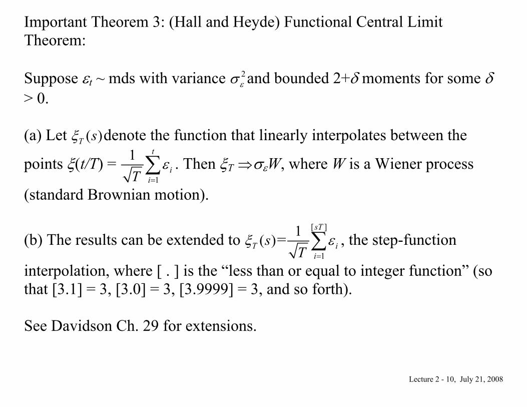
Important Theorem 3: (Hall and Heyde) Functional Central Limit Theorem: Suppose εt ~ mds with variance 2

εσ and bounded 2+δ moments for some δ > 0. (a) Let ( )T sξ denote the function that linearly interpolates between the

points ξ(t/T) = 1

1 t

iiTε

=∑ . Then ξT ⇒σεW, where W is a Wiener process

(standard Brownian motion).

(b) The results can be extended to ( )T sξ =[ ]

1

1 sT

iiTε

=∑ , the step-function

interpolation, where [ . ] is the “less than or equal to integer function” (so that [3.1] = 3, [3.0] = 3, [3.9999] = 3, and so forth). See Davidson Ch. 29 for extensions.

Lecture 2 - 11, July 21, 2008

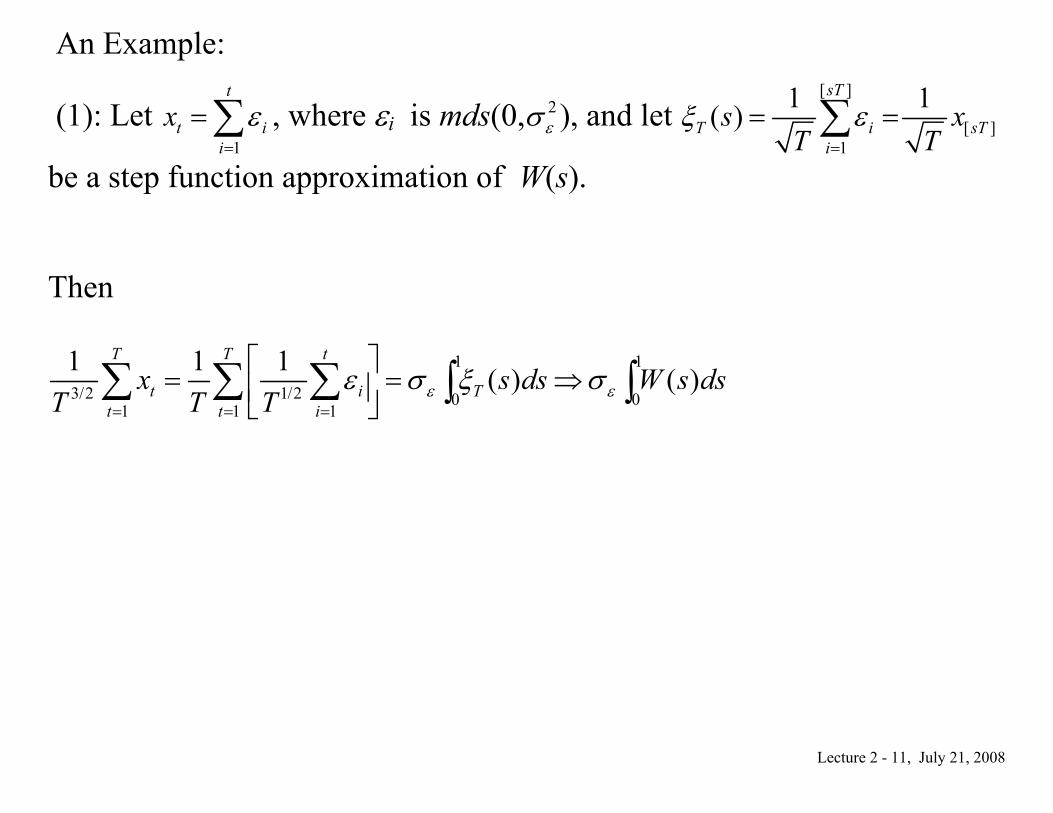
An Example:

(1): Let 1

t

t ii

x ε=

=∑ , where εi is mds(0, 2εσ ), and let

[ ]

[ ]1

1 1( )sT

T i sTi

s xT T

ξ ε=

= =∑

be a step function approximation of W(s). Then

1 1

3 2 1/2 0 01 1 1

1 1 1 ( ) ( )T T t

t i Tt t i

x s ds W s dsT T T ε εε σ ξ σ/

= = =

⎡ ⎤= = ⇒⎢ ⎥⎣ ⎦

∑ ∑ ∑ ∫ ∫

Lecture 2 - 12, July 21, 2008

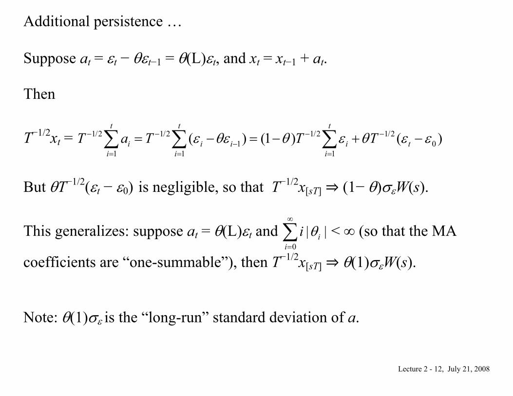
Additional persistence … Suppose at = εt − θεt−1 = θ(L)εt, and xt = xt−1 + at. Then

T−1/2xt = 1/2 1/2 1/2 1/21 0

1 1 1( ) (1 ) ( )

t t t

i i i i ti i i

T a T T Tε θε θ ε θ ε ε− − − −−

= = =

= − = − + −∑ ∑ ∑

But θT−1/2(εt − ε0) is negligible, so that T−1/2x[sT] (1− θ)σεW(s).

This generalizes: suppose at = θ(L)εt and 0

| |ii

i θ∞

=∑ < ∞ (so that the MA

coefficients are “one-summable”), then T−1/2x[sT] θ(1)σεW(s).  Note: θ(1)σε is the “long-run” standard deviation of a.

Lecture 2 - 13, July 21, 2008

What does this all mean? Suppose I want to approximate the 95th quantile of the distribution of, say,

vT = 3 21

1 T

tt

xT /

=∑ . Because vT

1

0( )v W s dsεσ= ∫ , I can use the 95th quantile of v

are the approximator. How do I find (or approximate) the 95th quantile of v?

Use Monte Carlo draws of 3/2

1 1

N t

it i

N zεσ−

= =∑∑ where zi ~ iidN(0,1) and N is

very large. This approximation works well when T is reasonably large, and does not require knowledge of the distribution of x.

Lecture 2 - 14, July 21, 2008

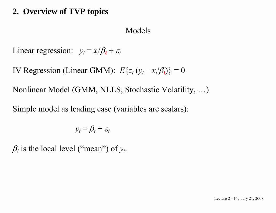
2. Overview of TVP topics

Models Linear regression: yt = xt′βt + εt IV Regression (Linear GMM): E{zt (yt – xt′βt)} = 0 Nonlinear Model (GMM, NLLS, Stochastic Volatility, …) Simple model as leading case (variables are scalars):

yt = βt + εt

βt is the local level (“mean”) of yt.

Lecture 2 - 15, July 21, 2008

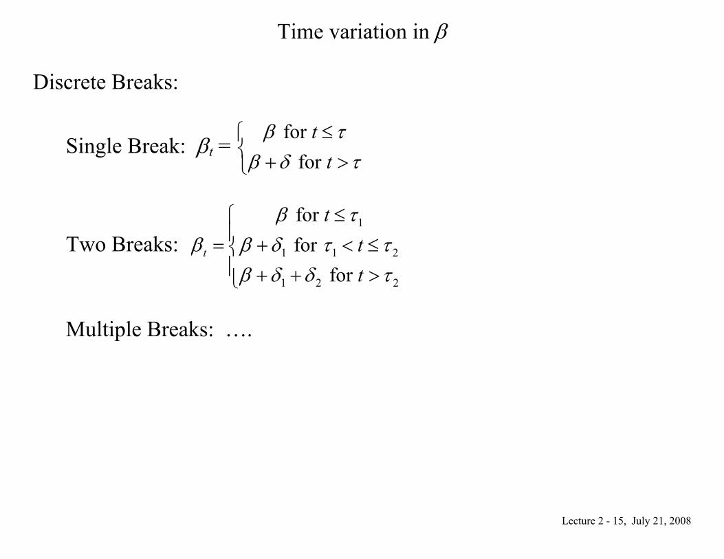
Time variation in β

Discrete Breaks:

Single Break: βt = for

for t

tβ τ

β δ τ≤⎧

⎨ + >⎩

Two Breaks: 1

1 1 2

1 2 2

for for

for t

ttt

β τβ β δ τ τ

β δ δ τ

≤⎧⎪= + < ≤⎨⎪ + + >⎩

Multiple Breaks: ….

Lecture 2 - 16, July 21, 2008

Stochastic Breaks/Markov Switching (Hamilton (1989)):

2-Regime Model:

βt = when 0

when 1t

t

ss

ββ δ

=⎧ ⎫⎨ ⎬+ =⎩ ⎭

,

st follows a Markov process P(st = i|st−1 = j) = pij

Multiple Regimes …

Other Stochastic Breaks: …

Lecture 2 - 17, July 21, 2008

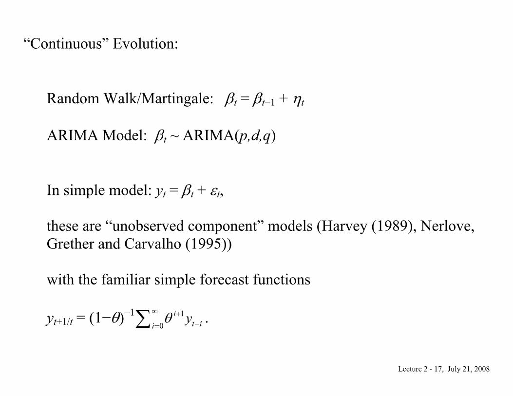
“Continuous” Evolution:

Random Walk/Martingale: βt = βt−1 + ηt ARIMA Model: βt ~ ARIMA(p,d,q) In simple model: yt = βt + εt, these are “unobserved component” models (Harvey (1989), Nerlove, Grether and Carvalho (1995)) with the familiar simple forecast functions yt+1/t = (1−θ)−1 1

0i

t iiyθ∞ +

−=∑ .

Lecture 2 - 18, July 21, 2008

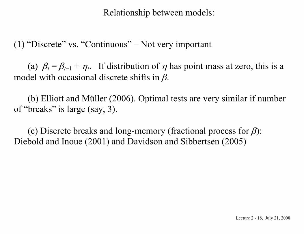
Relationship between models:

(1) “Discrete” vs. “Continuous” – Not very important (a) βt = βt−1 + ηt. If distribution of η has point mass at zero, this is a model with occasional discrete shifts in β. (b) Elliott and Müller (2006). Optimal tests are very similar if number of “breaks” is large (say, 3). (c) Discrete breaks and long-memory (fractional process for β): Diebold and Inoue (2001) and Davidson and Sibbertsen (2005)

Lecture 2 - 19, July 21, 2008

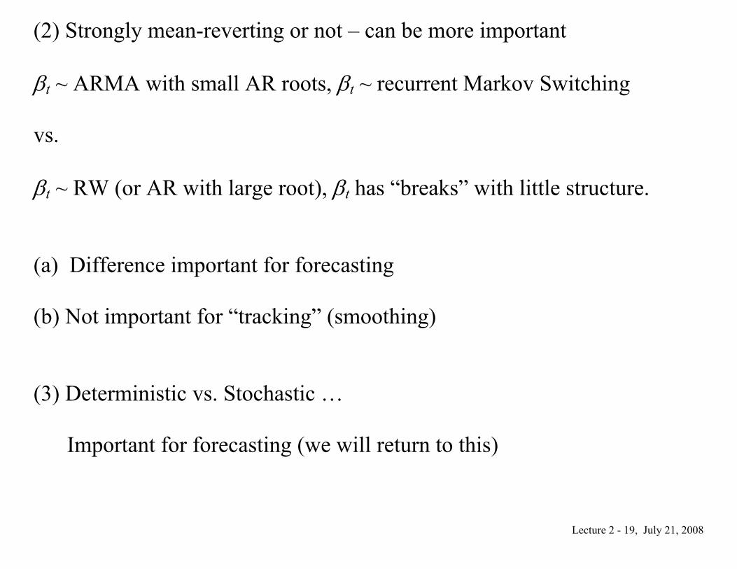
(2) Strongly mean-reverting or not – can be more important βt ~ ARMA with small AR roots, βt ~ recurrent Markov Switching vs. βt ~ RW (or AR with large root), βt has “breaks” with little structure. (a) Difference important for forecasting (b) Not important for “tracking” (smoothing) (3) Deterministic vs. Stochastic …

Important for forecasting (we will return to this)

Lecture 2 - 20, July 21, 2008

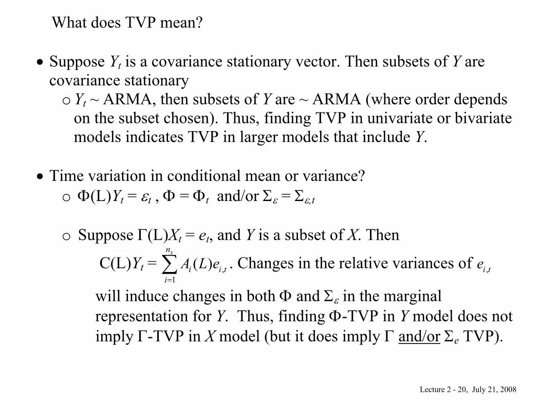
What does TVP mean? • Suppose Yt is a covariance stationary vector. Then subsets of Y are

covariance stationary o Yt ~ ARMA, then subsets of Y are ~ ARMA (where order depends

on the subset chosen). Thus, finding TVP in univariate or bivariate models indicates TVP in larger models that include Y.

• Time variation in conditional mean or variance? o Φ(L)Yt = εt , Φ = Φt and/or Σε = Σε,t

o Suppose Γ(L)Xt = et, and Y is a subset of X. Then

C(L)Yt = ,1

( )xn

i i ti

A L e=∑ . Changes in the relative variances of ,i te

will induce changes in both Φ and Σε in the marginal representation for Y. Thus, finding Φ-TVP in Y model does not imply Γ-TVP in X model (but it does imply Γ and/or Σe TVP).

Lecture 2 - 21, July 21, 2008

Evidence on TVP in Macro

• VARs o SW (1996): 5700 Bivariate VARs involving Post-war U.S. macro

series. Reject null of constant VAR coefficient (Φ) in over 50% of cases using tests with size = 10%.

o Many others …

• Volatility (Great Moderation)

Lecture 2 - 22, July 21, 2008

2. Testing Problems

Tests for a break Model: yt = βt + εt, where εt ~ iid (0, 2

εσ )

βt = for

for t

tβ τ

β δ τ≤⎧

⎨ + >⎩

Null and alternative: Ho: δ = 0 vs. Ho: δ ≠ 0 Tests for Ho vs. Ha depends on whether τ is known or unknown.

Lecture 2 - 23, July 21, 2008

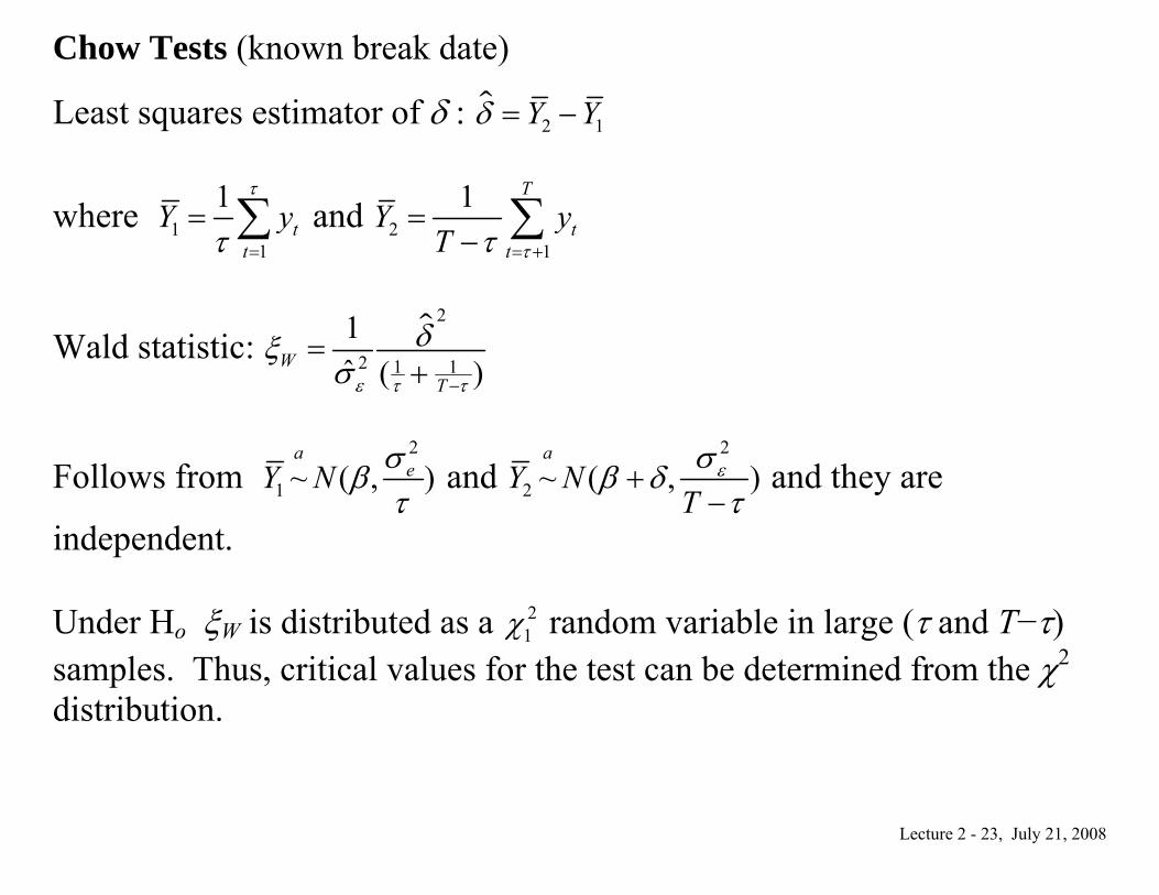
Chow Tests (known break date)

Least squares estimator of δ : 2 1Y Yδ = −

where 11

1t

tY y

τ

τ =

= ∑ and 21

1 T

tt

Y yT ττ = +

=− ∑

Wald statistic: 2

2 1 1

1ˆ ( )W

Tε τ τ

δξσ −

=+

Follows from 2

1 ~ ( )a

eY N σβτ

, and 2

2 ~ ( )a

Y NT

εσβ δτ

+ ,−

and they are

independent. Under Ho ξW is distributed as a 2

1χ random variable in large (τ and T−τ) samples. Thus, critical values for the test can be determined from the χ2 distribution.

Lecture 2 - 24, July 21, 2008

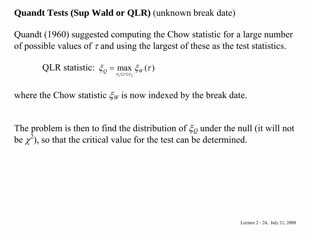
Quandt Tests (Sup Wald or QLR) (unknown break date)

Quandt (1960) suggested computing the Chow statistic for a large number of possible values of τ and using the largest of these as the test statistics.

QLR statistic:

1 2

max ( )Q Wτ τ τξ ξ τ

≤ ≤=

where the Chow statistic ξW is now indexed by the break date. The problem is then to find the distribution of ξQ under the null (it will not be χ2), so that the critical value for the test can be determined.

Lecture 2 - 25, July 21, 2008

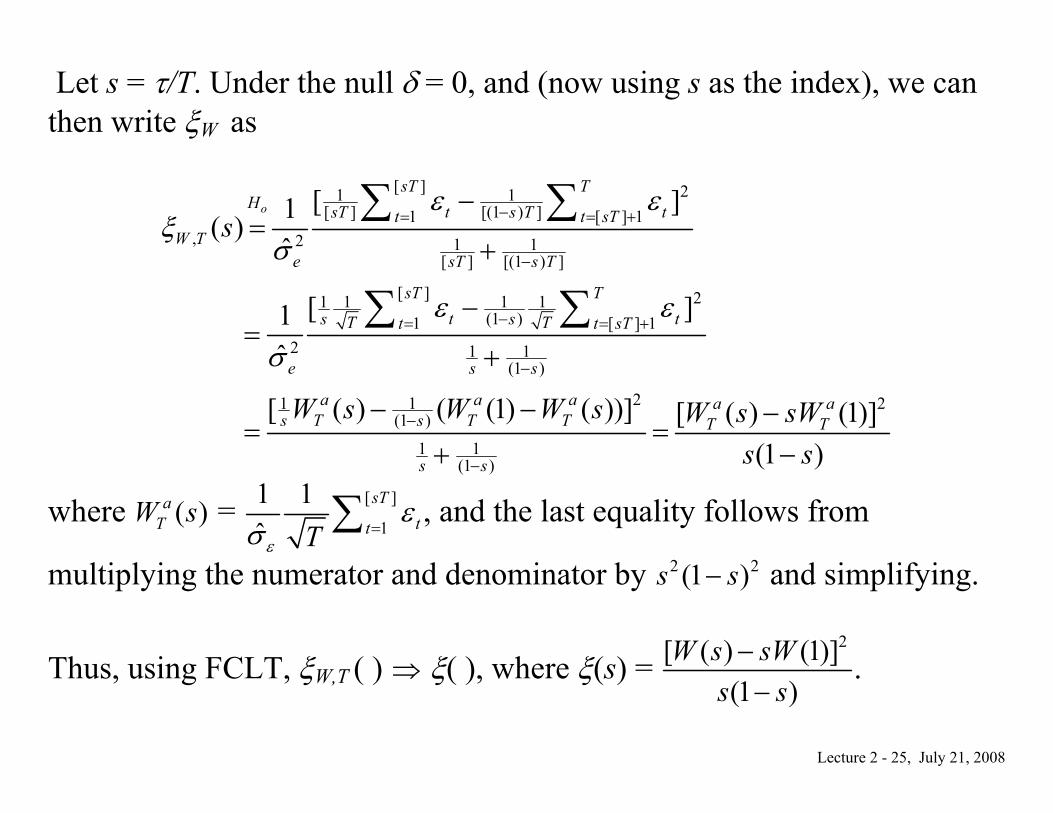
Let s = τ/T. Under the null δ = 0, and (now using s as the index), we can then write ξW as

[ ] 21 1[ ] [(1 ) ]1 [ ] 1

, 2 1 1[ ] [(1 ) ]

[ ] 21 1 1 1(1 )1 [ ] 1

2 1 1(1 )

2 21 1(1 )

1 1(1 )

[ ]1( )ˆ

[ ]1ˆ

[ ( ) ( (1) ( ))] [ ( ) (1)](1 )

o

sT TH t tsT s Tt t sT

W Te sT s T

sT Tt ts sT Tt t sT

e s s

a a a a aT T Ts s T T

s s

s

W s W W s W s sWs s

ε εξ

σ

ε ε

σ

−= = +

−

−= = +

−

−

−

−=

+

−=

+

− − −= =

+ −

∑ ∑

∑ ∑

where ( )aTW s = [ ]

1

1 1ˆ

sTttTε

εσ =∑ , and the last equality follows from

multiplying the numerator and denominator by 2 2(1 )s s− and simplifying.

Thus, using FCLT, ξW,T ( ) ⇒ ξ( ), where ξ(s) = 2[ ( ) (1)]

(1 )W s sW

s s−−

.

Lecture 2 - 26, July 21, 2008

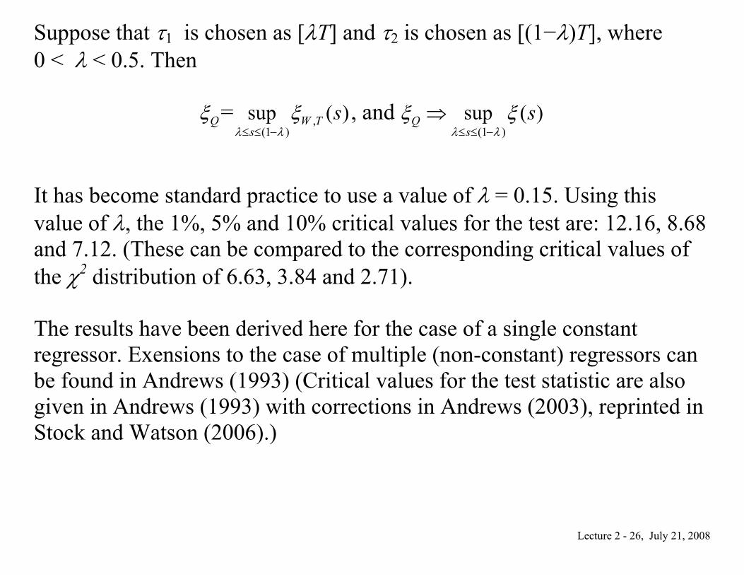
Suppose that τ1 is chosen as [λT] and τ2 is chosen as [(1−λ)T], where 0 < λ < 0.5. Then

Qξ = ,(1 )

sup ( )W Ts

sλ λ

ξ≤ ≤ −

, and (1 )

sup ( )Qs

sλ λ

ξ ξ≤ ≤ −

⇒

It has become standard practice to use a value of λ = 0.15. Using this value of λ, the 1%, 5% and 10% critical values for the test are: 12.16, 8.68 and 7.12. (These can be compared to the corresponding critical values of the χ2 distribution of 6.63, 3.84 and 2.71). The results have been derived here for the case of a single constant regressor. Exensions to the case of multiple (non-constant) regressors can be found in Andrews (1993) (Critical values for the test statistic are also given in Andrews (1993) with corrections in Andrews (2003), reprinted in Stock and Watson (2006).)

Lecture 2 - 27, July 21, 2008

Optimal Tests when the break point (τ) is unknown The QLR test seems very sensible, but is there a more powerful procedure? Andrews and Ploberger (1993) develop optimal tests (most powerful) for this (and related) problems. Recall the Neyman-Pearson (NP) lemma: consider two simple hypotheses Ho: Y ~ fo(y) vs. Ha: Y ~ fa(y), then the most powerful test rejects Ho for large values of the Likelihood Ratio, LR = fa(Y)/fo(Y), the ratio of the densities evaluated at the realized value of the random variable. Here: likelihoods depend on parameters δ, β, σε, and τ, where δ = 0 under Ho). (δ, β, σε) are easily handled in the NP framework. τ is more of a problem. It is unknown, and if Ho is true, it is irrelevant (τ is “unidentified” under the null). Andrews and Ploberger (AP) attack this problem.

Lecture 2 - 28, July 21, 2008

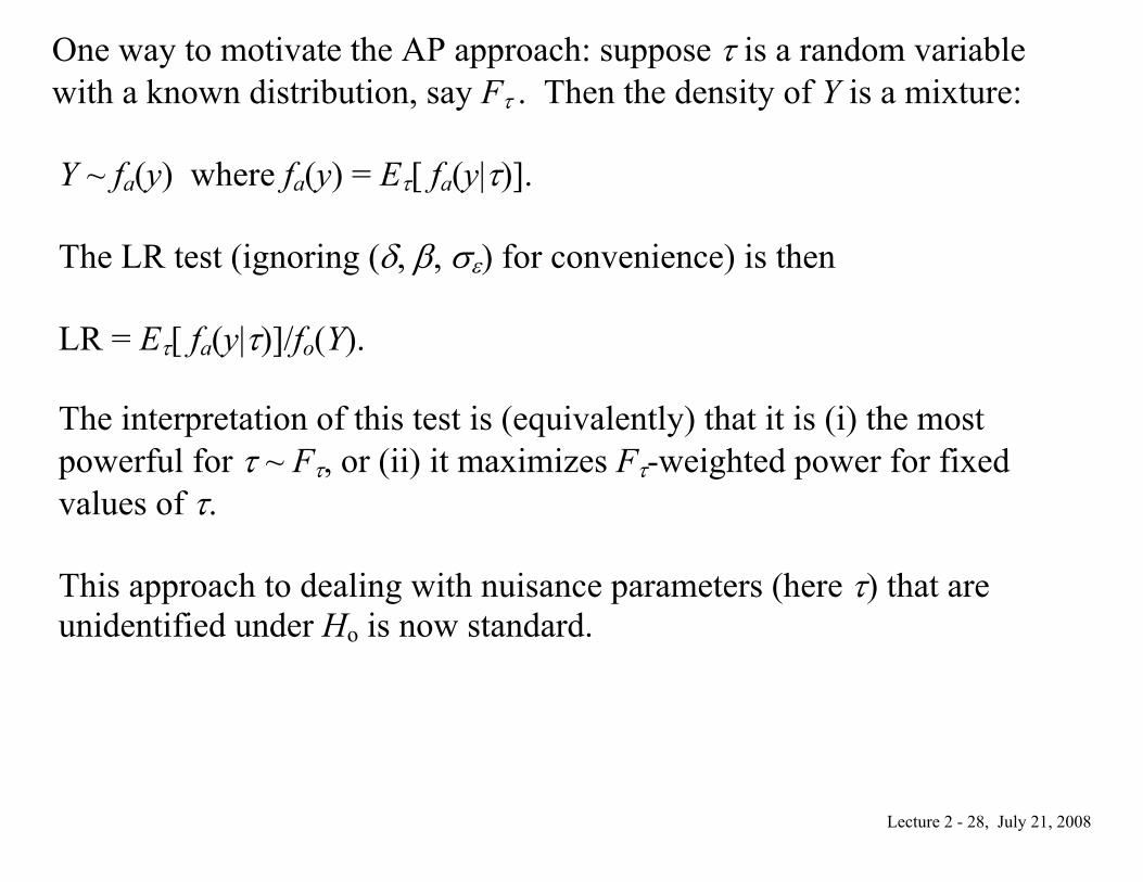
One way to motivate the AP approach: suppose τ is a random variable with a known distribution, say Fτ . Then the density of Y is a mixture: Y ~ fa(y) where fa(y) = Eτ[ fa(y|τ)]. The LR test (ignoring (δ, β, σε) for convenience) is then LR = Eτ[ fa(y|τ)]/fo(Y). The interpretation of this test is (equivalently) that it is (i) the most powerful for τ ~ Fτ, or (ii) it maximizes Fτ-weighted power for fixed values of τ. This approach to dealing with nuisance parameters (here τ) that are unidentified under Ho is now standard.

Lecture 2 - 29, July 21, 2008

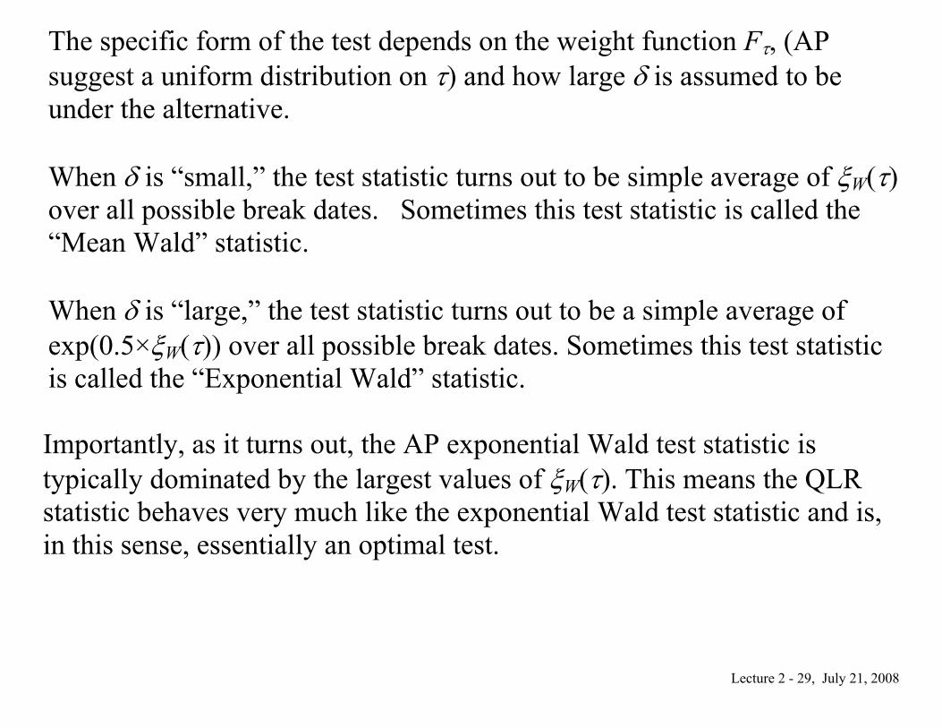
The specific form of the test depends on the weight function Fτ, (AP suggest a uniform distribution on τ) and how large δ is assumed to be under the alternative. When δ is “small,” the test statistic turns out to be simple average of ξW(τ) over all possible break dates. Sometimes this test statistic is called the “Mean Wald” statistic. When δ is “large,” the test statistic turns out to be a simple average of exp(0.5×ξW(τ)) over all possible break dates. Sometimes this test statistic is called the “Exponential Wald” statistic. Importantly, as it turns out, the AP exponential Wald test statistic is typically dominated by the largest values of ξW(τ). This means the QLR statistic behaves very much like the exponential Wald test statistic and is, in this sense, essentially an optimal test.

Lecture 2 - 30, July 21, 2008

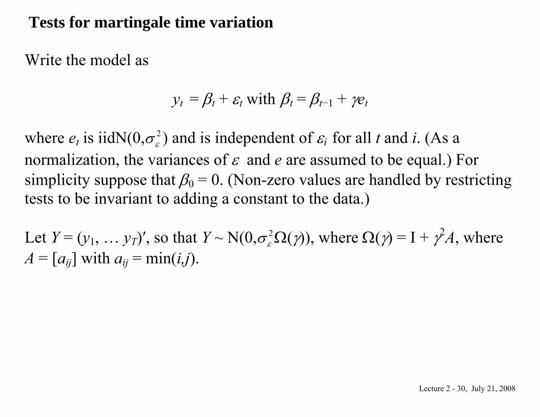
Tests for martingale time variation Write the model as

yt = βt + εt with βt = βt−1 + γet where et is iidN(0, 2

εσ ) and is independent of εi for all t and i. (As a normalization, the variances of ε and e are assumed to be equal.) For simplicity suppose that β0 = 0. (Non-zero values are handled by restricting tests to be invariant to adding a constant to the data.) Let Y = (y1, … yT)′, so that Y ~ N(0, 2

εσ Ω(γ)), where Ω(γ) = I + γ2A, where A = [aij] with aij = min(i,j).

Lecture 2 - 31, July 21, 2008

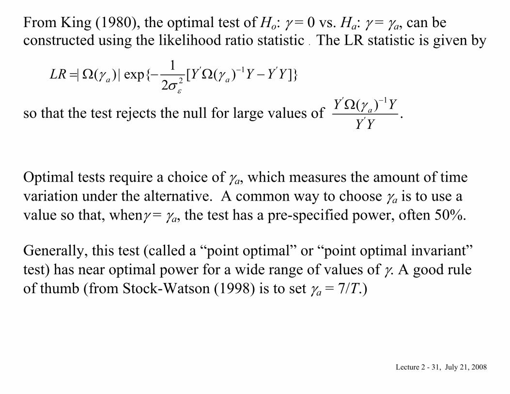
From King (1980), the optimal test of Ho: γ = 0 vs. Ha: γ = γa, can be constructed using the likelihood ratio statistic . The LR statistic is given by

12

1( ) exp{ [ ( ) ]}2a aLR Y Y Y Y

ε

γ γσ

′ − ′=| Ω | − Ω −

so that the test rejects the null for large values of 1( )aY Y

Y Yγ′ −

′

Ω .

Optimal tests require a choice of γa, which measures the amount of time variation under the alternative. A common way to choose γa is to use a value so that, whenγ = γa, the test has a pre-specified power, often 50%. Generally, this test (called a “point optimal” or “point optimal invariant” test) has near optimal power for a wide range of values of γ. A good rule of thumb (from Stock-Watson (1998) is to set γa = 7/T.)

Lecture 2 - 32, July 21, 2008

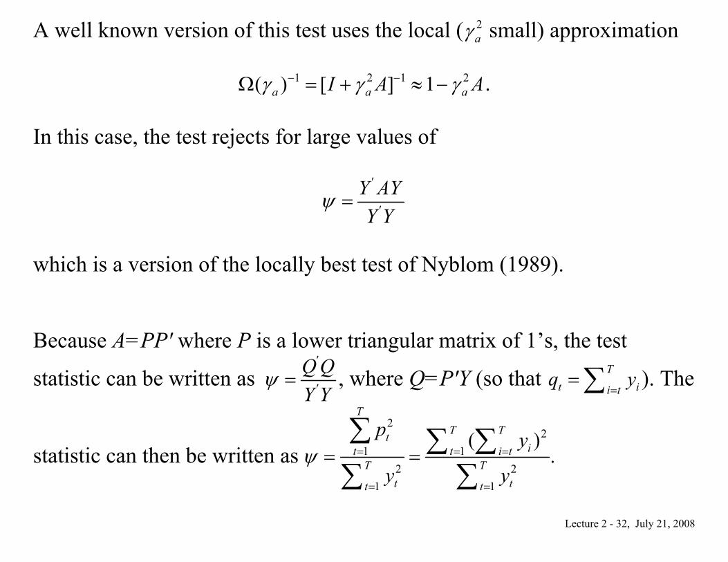
A well known version of this test uses the local ( 2aγ small) approximation

1 2 1 2( ) [ ] 1a a aI A Aγ γ γ− −Ω = + ≈ − .

In this case, the test rejects for large values of

Y AYY Y

ψ′

′=

which is a version of the locally best test of Nyblom (1989). Because A=PP′ where P is a lower triangular matrix of 1’s, the test

statistic can be written as Q QY Y

ψ′

′= , where Q=P′Y (so that Tt ii t

q y=

=∑ ). The

statistic can then be written as 2

21 1

2 21 1

( )T

T Ttit t i t

T Tt tt t

p y

y yψ = = =

= =

= = .∑ ∑ ∑∑ ∑

Lecture 2 - 33, July 21, 2008

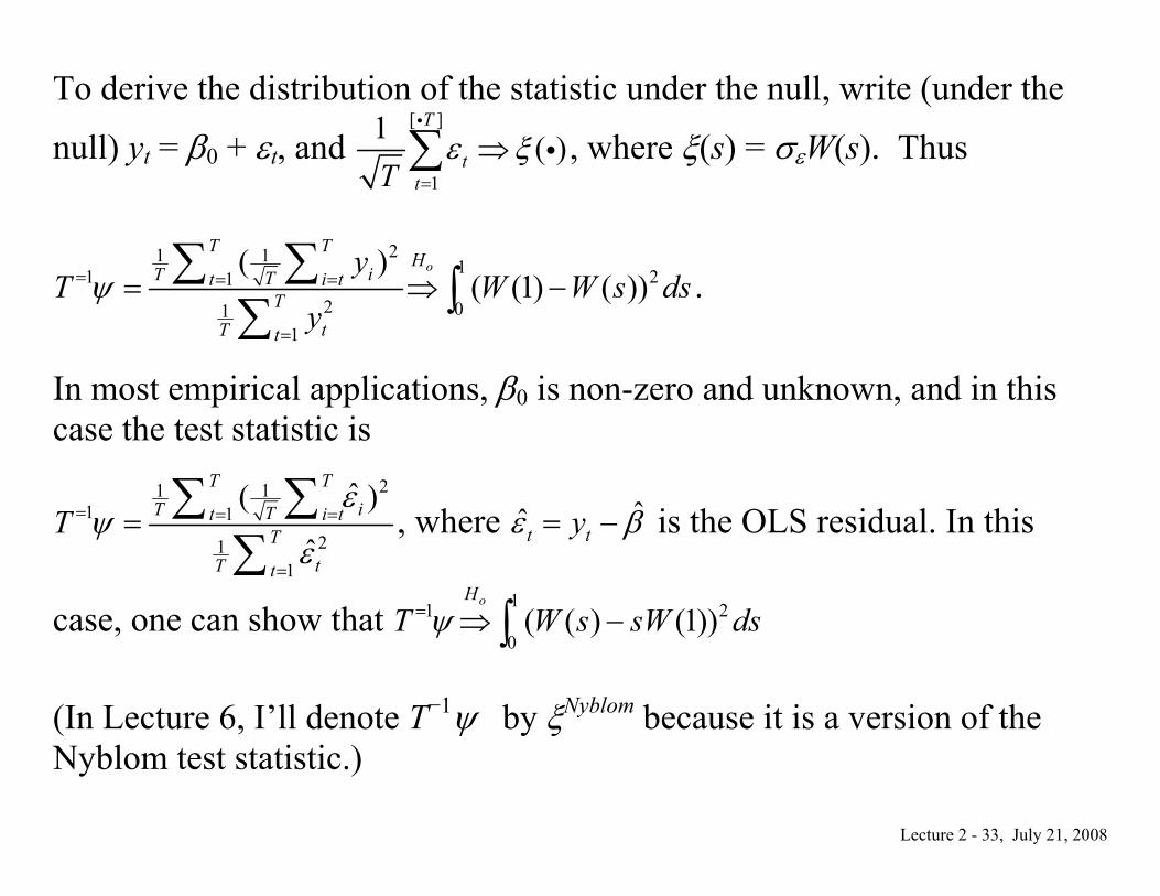
To derive the distribution of the statistic under the null, write (under the

null) yt = β0 + εt, and [ ]

1

1 ( )T

ttTε ξ

=

⇒∑i

i , where ξ(s) = σεW(s). Thus

21 1 11 21

2 011

( )( (1) ( ))

oT T

HiT Tt i t

TtT t

yT W W s ds

yψ= = =

=

= ⇒ −∑ ∑∫∑

.

In most empirical applications, β0 is non-zero and unknown, and in this case the test statistic is

21 11 1

211

ˆ( )

ˆ

T TiT Tt i t

TtT t

Tε

ψε

= = =

=

= ∑ ∑∑

, where ˆt̂ tyε β= − is the OLS residual. In this

case, one can show that 11 2

0( ( ) (1))

oH

T W s sW dsψ= ⇒ −∫ (In Lecture 6, I’ll denote T−1ψ by ξNyblom because it is a version of the Nyblom test statistic.)

Lecture 2 - 34, July 21, 2008

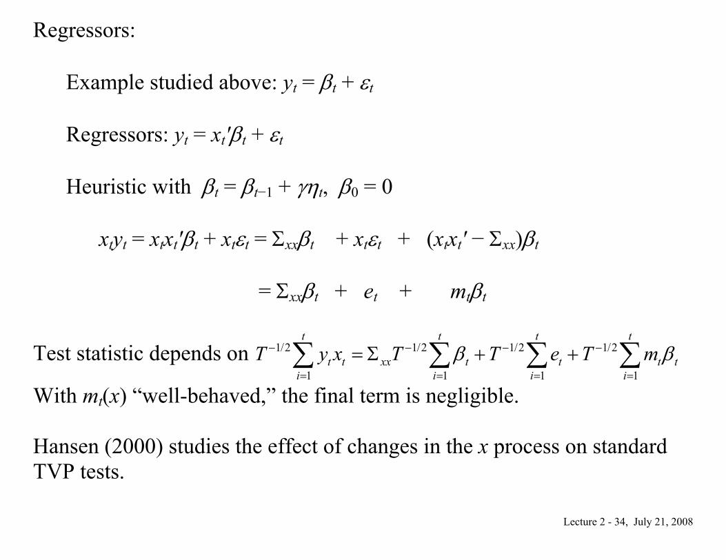
Regressors: Example studied above: yt = βt + εt Regressors: yt = xt′βt + εt Heuristic with βt = βt−1 + γηt, β0 = 0 xtyt = xtxt′βt + xtεt = Σxxβt + xtεt + (xtxt′ − Σxx)βt = Σxxβt + et + mtβt

Test statistic depends on 1/2 1/2 1/2 1/2

1 1 1 1

t t t t

t t xx t t t ti i i i

T y x T T e T mβ β− − − −

= = = =

= Σ + +∑ ∑ ∑ ∑

With mt(x) “well-behaved,” the final term is negligible. Hansen (2000) studies the effect of changes in the x process on standard TVP tests.

Lecture 2 - 35, July 21, 2008

HAC Corrections: yt = xt′βt + εt where Var(xtεt) ≠ 2

εσ ΣXX.

Lecture 2 - 36, July 21, 2008

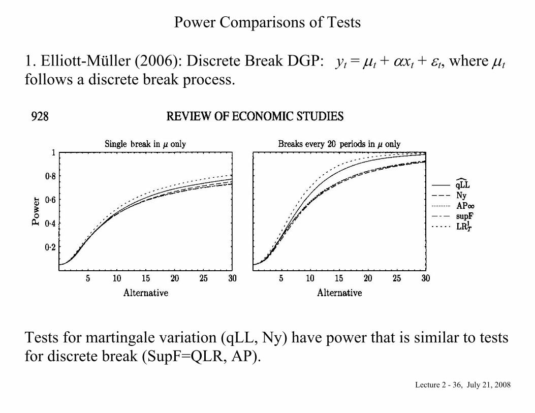
Power Comparisons of Tests 1. Elliott-Müller (2006): Discrete Break DGP: yt = μt + αxt + εt, where μt follows a discrete break process.

Tests for martingale variation (qLL, Ny) have power that is similar to tests for discrete break (SupF=QLR, AP).

Lecture 2 - 37, July 21, 2008

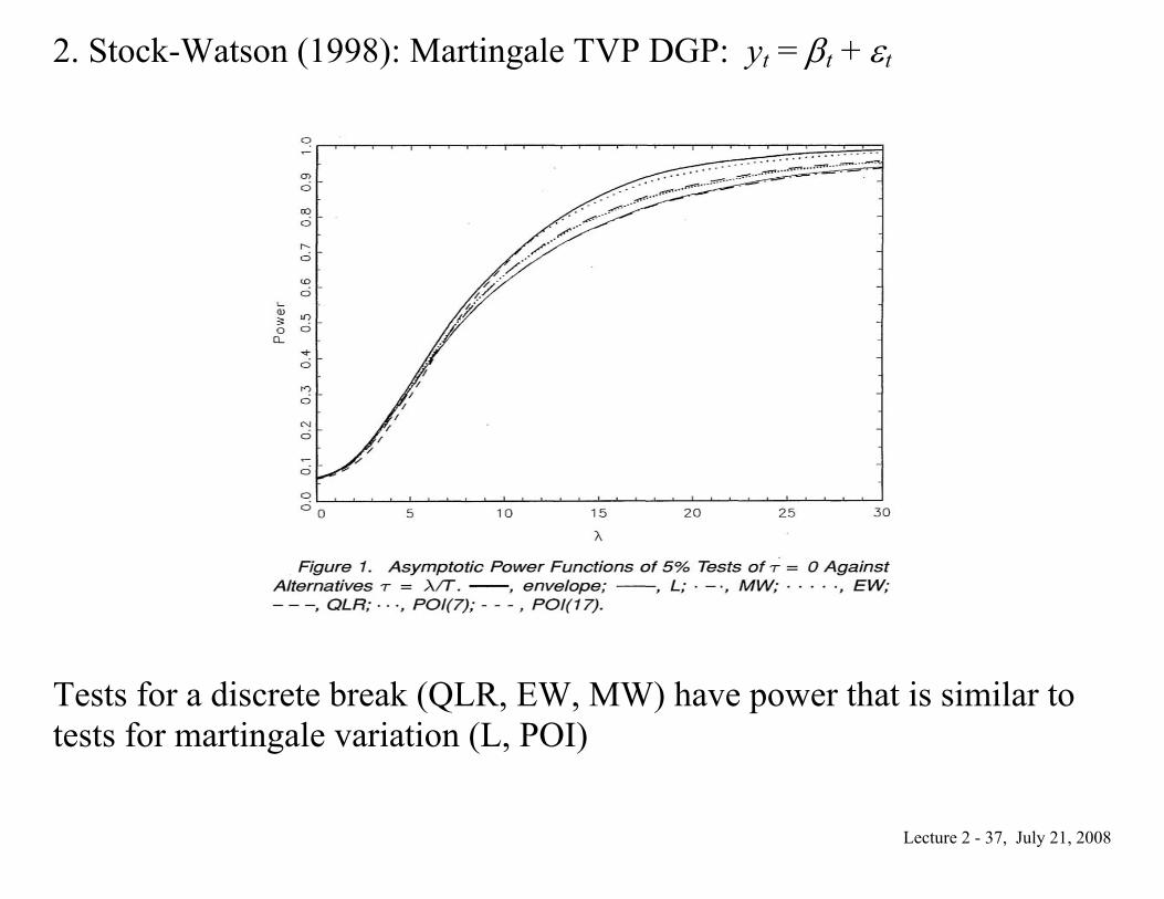
2. Stock-Watson (1998): Martingale TVP DGP: yt = βt + εt

Tests for a discrete break (QLR, EW, MW) have power that is similar to tests for martingale variation (L, POI)

Lecture 2 - 38, July 21, 2008

Summary

1.FCLT (tool)

2.Overview of TVP topics

a. Persistent vs. mean reverting TVP

3.Testing problems

a. Discrete break and AP approach

4.Tests

a. Little difference between tests for discrete break and persistent “continuous” variation. What do you conclude when the null of stability is rejected?