U.S. Department of the Interior

U.S. Geological Survey

Steve Foga1, Brian Davis1, Brian Sauer2, John Dwyer2

1 SGT Inc., contractor to USGS EROS Center2 USGS EROS Center

GSA 2016 – Denver, CO

The Future of Landsat Data Products:

Analysis Ready Data and Essential

Climate Variables

Outline

Status Quo

Essential Climate Variables

Data Improvements

Collections

Analysis Ready Data

Use Cases

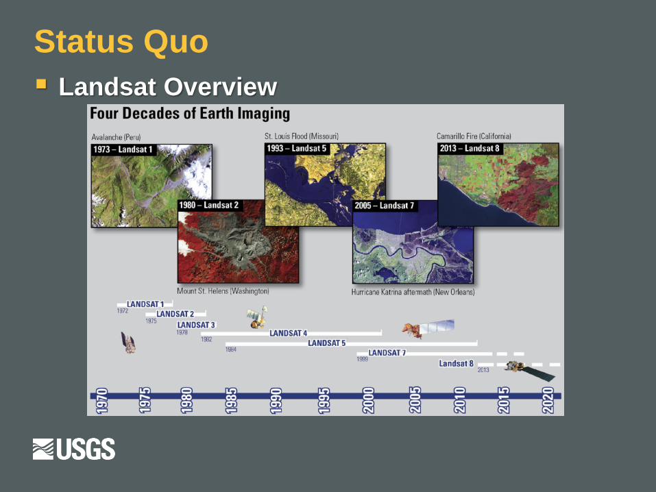
Status Quo

Landsat Overview

Status Quo Landsat Bandpasses

MSS = Multispectral Scanner (Landsat 1-5); TM = Thematic Mapper (Landsat 4-5); ETM+ = Enhanced Thematic

Mapper Plus (Landsat 7); OLI = Operational Land Imager (Landsat 8); TIRS = Thermal Infrared Sensor (Landsat

8)

Status Quo Development of higher level data

products

Surface Reflectance (SR)

Future: land surface temperature

EROS Science Processing Architecture

(ESPA)

Higher level data products, data

customization, statistics

On Demand Interface (ODI)

Application Programming Interface (API)

Order options

Vegetation/burn indices

Top of Atmosphere Reflectance, SR, cloud

masks

Reprojection, spatial subset, pixel resizing,

multiple formats

Order interface layout in ESPA.

Status Quo

Data in a “scene”-based format

Covers ~180 km2 of land

The extent of a single Landsat scene in relation to CONUS.

Essential Climate Variables PIs across USGS

Physical parameters derived from SR

Dynamic Surface Water Extent (DSWE;

Jones, 2015 [1])

Burned Area (BA; Hawbaker et al., 2016 [2])

Fractional Snow Covered Area (fSCA;

Selkowitz, 2015 [3])Dynamic Surface Water Extent (DSWE) probability product

shown over glacier lakes in North-central North Dakota.

Burned Area (BA) classification map over burn scar in

California. Product also comes as probability product.Fractional Snow Covered Area probability product and

related validation methodology. From Selkowitz, 2015 [3].

Data Improvements

Landsat Collections

Buckets known as data tiers

Consistent radiometry, threshold of scene-wide geometry

Tier 1 enables stackability

Best data can be easily accessed without additional metadata

harvesting

Tier Geometric

RMSE

Radiometric % OLI/TIRS % ETM+ TM

1 ≤ 12m Static 60.42%* 74.98% 65.41%

2 > 12m Static 39.58% 25.02% 34.59%

RT ** Recently acquired data with preliminary geometry and radiometry information.

Will eventually become Tier 1 or Tier 2. * Many OLI/TIRS scenes do not reach geometric threshold due to imaging of oceans, where ground control points (GCP)

are often not sufficient.

** RT = “Real Time”

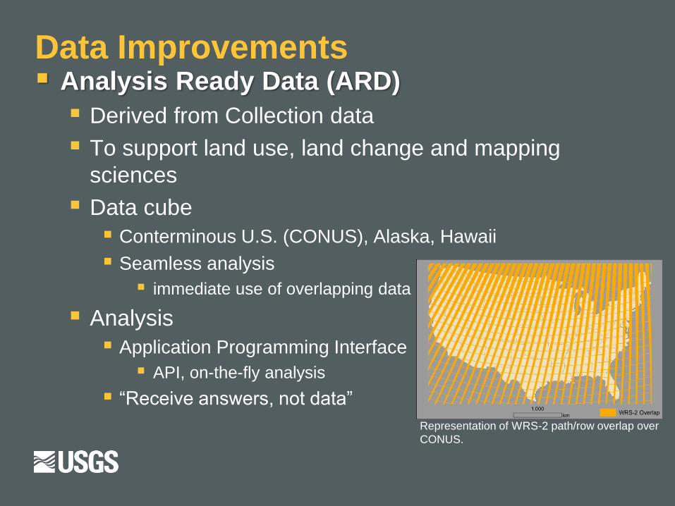
Data Improvements Analysis Ready Data (ARD)

Derived from Collection data

To support land use, land change and mapping

sciences

Data cube

Conterminous U.S. (CONUS), Alaska, Hawaii

Seamless analysis

immediate use of overlapping data

Analysis

Application Programming Interface

API, on-the-fly analysis

“Receive answers, not data”

Representation of WRS-2 path/row overlap over

CONUS.

Data Improvements

ARD Specifications

USGS Analysis Ready Dataset (ARD) Product Projection Parameters

Projection: Albers Equal Area Conic

Datum: North American Datum 1983 (NAD83)

Conterminous U.S. Alaska Hawaii

First standard parallel 29.5˚ 55.0˚ 8.0˚

Second standard parallel 45.5˚ 65.0˚ 18.0˚

Longitude of central

meridian-96.0˚ -154.0˚ -157.0˚

Latitude of projection

origin23.0˚ 50.0˚ 3.0˚

False Easting 0.0 0.0 0.0

False Northing 0.0 0.0 0.0

Use cases Quick visualization

Filter pixels by quality assurance (QA) bit(s)

Cloud, cloud shadow, snow/ice (below)

Saturation, dropped frames, terrain occlusion

Best pixel by index and/or threshold

Series of tests to create probability map(s)

Composite bands to accentuate features

Cloud masking product delivered with Landsat 8 surface reflectance data.

Image was acquired over Yellowstone National Park, Wyoming.

Use cases

Lithology, Hydrothermal

Alteration maps Color composites of band ratios

(right) to show areas of potential

alteration

Goldfield mining district, NV, based

upon work by Sabins, 1999 [4]

Use of spectral unmixing (e.g.,

Principal Components Analysis

(PCA)) to abstract distinct

signatures using all bands

Band ratio composite using L8 surface refl. data detailing

potential hydrothermal alteration (yellow/orange) in Nevada.

Use cases Sensor compatibility across time

Red, Near Infrared (NIR), Shortwave Infrared (SWIR) 1, SWIR2

narrowed from TM/ETM+ to OLI

Quick analysis at hydrothermally altered area near Drum Mountain, Utah

Sensors still detect same features, thus are cross-comparable

Use cases Derive glacier velocities with feature tracking

Landsat 8 OLI ideal for this

High signal-to-noise ratio (SNR)

High enough to track snow drifts [5], not just crevasses

15m panchromatic bands (sharper detail)

Repeat imaging opportunities

Converging fields of view with polar orbit

Ascending node imaging during midnight sun at poles

Seamless base image creation with ARD

Velocity profile of southern Alaska glaciers, derived from OLI images.

Borrowed from Fahnestock et al., 2015 [5].

Use cases Hazards

Quickly compile time series to show before/after

Composite with SWIR to reduce smoke (below)

Holuhraun lava flow in Iceland captured by Landsat 8. Left: SWIR,NIR,green composite. Center: red,green,blue composite. Right: thermal. Image

modified from http://eros.usgs.gov/imagegallery/image-week-2#Iceland_images.

Before (left) and after (right) of landslide at Glacier Bay National Park and Preserve in Alaska captured by Landsat 8.

Resources

Landsat mission webpage:

http://landsat.usgs.gov

Collections:

http://landsat.usgs.gov/landsatcollections.php

Landsat data: http://earthexplorer.usgs.gov/

EROS Science Processing Architecture

(ESPA): https://espa.cr.usgs.gov/

References

[1] Jones, J. W. (2015). Efficient wetland surface water detection and monitoring via Landsat:

Comparison with in situ data from the Everglades Depth Estimation Network. Remote

Sensing, 7(9), 12503-12538.

[2] Hawbaker, T., Vanderhoof, M., French, N., Billmire, M., Beal, Y. J. G., Takacs, J., ... & Caldwell,

M. (2016, April). Automated mapping of burned areas in Landsat imagery; tracking spatial and

temporal patterns of burned areas and greenhouse gas emissions in the Southern Rocky

Mountains, USA. In EGU General Assembly Conference Abstracts (Vol. 18, p. 10709).

[3] Selkowitz, D. (2015, December). The USGS Landsat Snow Covered Area Science Data

Products. In 2015 AGU Fall Meeting. Agu. Image accessed 01 AUG 2016 from

http://landsat.gsfc.nasa.gov/?p=11702.

[4] Sabins, F. F. (1999). Remote sensing for mineral exploration. Ore Geology Reviews, 14(3),

157-183.

[5] Fahnestock, M., Scambos, T., Moon, T., Gardner, A., Haran, T., & Klinger, M. (2015). Rapid

large-area mapping of ice flow using Landsat 8. Remote Sensing of Environment.