the generalized weighted lindley distribution: properties ... · generalizations of the lindley...
TRANSCRIPT
The Generalized Weighted Lindley Distribution:Properties, Estimation and Applications
P. L. RAMOS,∗ F. LOUZADA†
Institute of Mathematical Science and ComputingUniversidade de Sao Paulo, Sao Carlos-SP, Brazil
January/2016
Abstract
In this paper, we proposed a new lifetime distribution namely generalized weightedLindley (GLW) distribution. The GLW distribution is a useful generalization of theweighted Lindley distribution, which accommodates increasing, decreasing, decreasing-increasing-decreasing, bathtub, or unimodal hazard functions, making the GWL dis-tribution a flexible model for reliability data. A significant account of mathematicalproperties of the new distribution are presented. Different estimation procedures arealso given such as, maximum likelihood estimators, method of moments, ordinary andweighted least-squares, percentile, maximum product of spacings and minimum dis-tance estimators. The different estimators are compared by an extensive numericalsimulations. Finally, we analyze two data sets for illustrative purposes, proving thatthe GWL outperform several usual three parameters lifetime distributions.Keywords: Generalized weighted Lindley distribution, Maximum Likelihood Estima-tion, Maximum product of spacings.
1 Introduction
In recent years, several new extensions of the exponential distribution has been introducedin the literature for describing real problems. Ghitany et al. (2008) investigated differentproperties of the Lindley distribution and outlined that in many cases the Lindley distri-bution is a better model than one based on the exponential distribution. Since then, many
∗Email: [email protected]†Email: [email protected]
1
arX
iv:1
601.
0741
0v2
[m
ath.
ST]
18
Jul 2
016

generalizations of the Lindley distribution have been introduced, such as generalized Lind-ley (Zalerzadeh and Dolati, 2009), extended Lindley (Bakouch et al., 2012), exponentialPoisson Lindley (Barreto-Souza and Bakouch, 2013), Power Lindley (Ghitany et al., 2013)distribution, among others.
Ghitany et al. (2011) introduced a new class of weighted Lindley (WL) distributionadding more flexibility to the Lindley distribution. Let T be a random variable with a WLdistribution the probability density function (p.d.f) is given by
f(t|λ, φ) =λφ+1
(λ+ φ)Γ(φ)tφ−1(1 + t)e−λt, (1)
for all t > 0 , φ > 0 and λ > 0 and Γ(φ) =∫∞
0e−xxφ−1dx is known as gamma function.
One of its peculiarities is that the hazard function can has an increasing (φ ≥ 1) or bathtub(0 < φ < 1) shape. Different properties of this model and estimation methods were studiedby Mazucheli et al. (2013), Ali (2013), Wang (2015), Al-Mutairi et al. (2015) among others.
In this paper, a new lifetime distribution family is proposed, which is an direct general-ization of the weighted Lindley distribution. The p.d.f is given by
f(t|φ, λ, α) =αλαφ
(λ+ φ)Γ(φ)tαφ−1(λ+ (λt)α)e−(λt)α , (2)
for all t > 0, φ > 0, λ > 0 and α > 0. Important probability distributions can be obtainedfrom the GWL distribution as the weighted Lindley distribution (α = 1) , Power Lindley dis-tribution (φ = 1) and the Lindley distribution (φ = 1 and α = 1). Due this relationship, suchmodel could also be named as weighted power Lindley or generalized power Lindley distribu-tion. We present a proof that this model has different forms of the hazard function, such as:increasing, decreasing, bathtub, unimodal or decreasing-increasing-decreasing shape, makingthe GWL distribution a flexible model for reliability data. Moreover, a significant accountof mathematical properties of the new distribution are provided.
The inferential procedures of the parameters of the GLW distribution are presented con-sidering different estimation methods such as: maximum likelihood estimators (MLE), meth-ods of moments (ME), ordinary least-squares estimation (OLSE), weighted least-squares es-timation (WLSE), maximum product of spacings (MPS), Cramer-von Mises type minimumdistance (CME), Anderson-Darling (ADE) and Right-tail Anderson-Darling (RADE). Wecompare the performances of the such different methods using extensive numerical simula-tions. Finally, we analyze two data sets for illustrative purposes, proving that the GWLoutperform several usual three parameters lifetime distributions such as: the generalizedGamma distribution (Stacy, 1962), the generalized Weibull (GW) distribution (Mudholkaret al., 1996), the generalized exponential-Poisson (GEP) distribution (Barreto-Souza andCribatari-Neto, 2009) and the exponentiated Weibull (EP) distribution (Mudholkar et al.,1995).
The paper is organized as follows. In Section 2, we provide a significant account ofmathematical properties of the new distribution. In Section 3, we discuss the eight estimation
2

methods considered in this paper. In Section 4 a simulation study is presented in order toidentify the most efficient procedure. In Section 5 the methodology is illustrated in two realdata sets. Some final comments are presented in Section 6.
2 Generalized Weighted Lindley distribution
The Generalized weighted Lindley distribution (2) can be expressed as a two-componentmixture
f(t|φ, λ, α) = pf1(t|φ, λ, α) + (1− p)f2(t|φ, λ, α)
where p = λ/(λ+φ) and Tj ∼ GG(φ+ j−1, λ, α), for j = 1, 2, i.e, fj(t|λ, φ) has GeneralizedGamma distribution, given by
fj(t|φ, λ, α) =α
Γ(φ+ j − 1)λα(φ+j−1)tα(φ+j−1)−1e−(λt)α . (3)
The behaviours of the p.d.f. (2) when t→ 0 and t→∞ are, respectively, given by
f(0) =
∞, if αφ < 1
αλ2
(λ+ φ)Γ(φ), if αφ = 1
0, if αφ > 1
, f(∞) = 0.
Figure 1 gives examples of the shapes of the density function for different values of φ, λand α.
0 1 2 3 4
0.0
0.5
1.0
1.5
t
f(t)
φ=0.2, λ=1.5, α=2.1φ=0.5, λ=1.5, α=1.5φ=0.7, λ=1.5, α=1.0φ=0.7, λ=1.5, α=1.5φ=3.5, λ=20, α=0.7
0 1 2 3 4
0.0
0.5
1.0
1.5
t
f(t)
φ=0.2, λ=2.5, α=0.2φ=0.5, λ=2.5, α=0.6φ=1.0, λ=2.5, α=0.8φ=1.5, λ=1.5, α=0.5φ=2.0, λ=1.5, α=1.2
Figure 1: Density function shapes for GWL distribution considering different values of φ, λand α.
3

The cumulative distribution function from the GWL distribution is given by
F (t|φ, λ, α) =γ [φ, (λt)α] (λ+ φ)− (λt)αφe−(λt)α
(λ+ φ)Γ(φ). (4)
where γ[y, x] =∫ x
0wy−1e−wdw is the lower incomplete gamma function.
2.1 Moments
Many important features and properties of a distribution can be obtained through its mo-ments, such as mean, variance, kurtosis and skewness. In this section, we present someimportant moments, such as the moment generating function, r-th moment, r-th centralmoment among others.
Theorem 2.1. For the random variable T with GWL distribution, the moment generatingfunction is given by
MX(t) =∞∑r=0
tr
λrr!
(rα
+ φ+ λ)
Γ( rα
+ φ)
(λ+ φ)Γ(φ). (5)
Proof. Note that, the moment generating function from GG distribution (3) is given by
MX,j(t) =∞∑r=0
tr
r!
Γ( rα
+ φ+ j − 1)
λrΓ(φ+ j − 1).
Therefore, as the GWL (2) distribution can be expressed as a two-component mixture,we have
MX(t) = E[etX]
=
∫ ∞0
etxf(x|φ, λ, α)dx = pMX,1(t) + (1− p)MX,2(t)
=λ
(λ+ φ)
∞∑r=0
tr
r!
Γ( rα
+ φ)
λrΓ(φ)+
φ
(λ+ φ)
∞∑r=0
tr
r!
Γ( rα
+ φ+ 1)
λrΓ(φ+ 1)
=1
(λ+ φ)
∞∑r=0
tr
r!
λΓ( rα
+ φ)
λrΓ(φ)+
1
(λ+ φ)
∞∑r=0
tr
r!
(rα
+ φ)
Γ( rα
+ φ)
λrΓ(φ)
=∞∑r=0
tr
λrr!
(rα
+ φ+ λ)
Γ( rα
+ φ)
(λ+ φ)Γ(φ).
Corollary 2.2. For the random variable T with GWL distribution, the r-th moment is givenby
µr = E[T r] =
(rα
+ φ+ λ)
Γ( rα
+ φ)
(λ+ φ)λrΓ(φ). (6)
4

Proof. From the literature µr = M(r)X (0) = dnMX(0)
dtnand the result follows.
Corollary 2.3. For the random variable T with GWL distribution, the r-th central momentis given by
Mr = E[T − µ]r =r∑i=0
(r
i
)(−µ)r−iE[T i]
=r∑i=0
(r
i
)(−(
1α
+ φ+ λ)
Γ(
1α
+ φ)
λ(λ+ φ)Γ(φ)
)r−i (iα
+ φ+ λ)
Γ( iα
+ φ)
(λ+ φ)λiΓ(φ)
(7)
Corollary 2.4. A random variable T with GWL distribution, has the mean and variancegiven by
µ =
(1α
+ φ+ λ)
Γ(
1α
+ φ)
λ(λ+ φ)Γ(φ), (8)
σ2 =λ(λ+ φ)
(2α
+ φ+ λ)
Γ(
2α
+ φ)−(
1α
+ φ+ λ)2
Γ(
1α
+ φ)2
λ2(λ+ φ)2Γ(φ)2. (9)
Proof. From (6) and considering r = 1 follows µ1 = µ. The second result follows from (7)considering r = 2 and with some algebra follow the results.
Different type of moments can be easily achieved for GWL distribution, one in particular,that has play a important role in information theory is given by
E[log(T )] =(ψ(φ)− α log λ+ (λ+ φ)−1)
α. (10)
2.2 Survival Properties
In this section, we present the survival, the hazard and mean residual life function for theGWL distribution. The survival function of T ∼ GWL(φ, λ, α) with the probability of anobservation does not fail until a specified time t is
S(t|φ, λ, α) =Γ [φ, (λt)α] (λ+ φ) + (λt)αφe−(λt)α
(λ+ φ)Γ(φ)(11)
where Γ(x, y) =∫ x
0wy−1e−xdw is called upper incomplete gamma. The hazard function
quantify the instantaneous risk of failure at a given time t and is given by
h(t|φ, λ, α) =f(t|φ, λ, α)
S(t|φ, λ, α)=
αλαφtαφ−1(λ+ (λt)α)e−(λt)α
Γ [φ, (λt)α] (λ+ φ) + (λt)αφe−(λt)α. (12)
5

The behaviours of the hazard function (12) when t → 0 and t → ∞, respectively, aregiven by
h(0) =
∞, if αφ < 1
αλ2
(λ+ φ)Γ(φ), if αφ = 1
0, if αφ > 1
and h(∞) =
0, if αφ < 1
λ, if αφ = 1
∞, if αφ > 1.
Theorem 2.5. The hazard rate function h(t) of the generalized weighted Lindley distributionis increasing, decreasing, bathtub, unimodal or decreasing-increasing-decreasing shaped.
Proof. Is not straightforward to apply the theorem proposed by Glaser (1980) in the GLWdistribution. Moreover, since the hazard rate function (12) is complex, we consider thefollowing cases:
1. Let α = 1, then GWL distribution reduces to the WL distribution. In this case,Ghitany et al. (2008) proved that the hazard function is bathtub shaped (increasing)if 0 < φ < 1 (φ > 0), for all λ > 0.
2. Let φ = 1, then GWL distribution reduces to the PL distribution. In this case,considering β = λα, Ghitany et al. (2013) proved that the hazard function is
• increasing if {0 < α ≥ 1, β > 0};• decreasing if
{0 < α ≤ 1
2, β > 0
}or{
12< α < 1, β ≥ (2α− 1)2(4α(1− α))−1};
• decreasing-increasing-decreasing if{
12< α < 1, 0 < β < (2α− 1)2(4α(1− α))−1}.
3. Let α = 2 and λ = 1, from Glasers theorem (1980), we conclude straightforwardly thatthe hazard rate function is decreasing shaped (unimodal) if 0 < φ < 1 (φ > 1).
These properties make the GWL distribution a flexible model for reliability data. Figure2 gives examples from the shapes of the hazard function for different values of φ, λ and α.
The mean residual life (MRL) has been used widely in survival analysis and represents theexpected additional lifetime given that a component has survived until time t, the followingresult presents the MRL function of the GWL distribution
Proposition 2.6. The mean residual life function r(t|φ, λ, α) of the GWL distribution isgiven by
r(t|φ, λ, α) =
(φ+ 1
α+ λ)
Γ(φ+ 1
α, (λt)α
)− λt(λ+ φ)Γ (φ, (λt)α)
λ[(λ+ φ)Γ(φ, (λt)α) + (λt)αφe−(λt)α ]. (13)
6

0 1 2 3 4
02
46
810
t
h(t)
φ=0.2, λ=1.5, α=2.1φ=0.5, λ=1.5, α=1.5φ=0.7, λ=1.5, α=1.0φ=0.7, λ=1.5, α=1.5φ=3.5, λ=20, α=0.7
0 1 2 3 4
01
23
45
6
t
h(t)
φ=0.2, λ=2.5, α=0.2φ=0.5, λ=2.5, α=0.6φ=1.0, λ=2.5, α=0.8φ=1.5, λ=1.5, α=0.5φ=2.0, λ=1.5, α=1.2
Figure 2: Hazard function shapes for GWL distribution and considering different values ofφ, λ and α
Proof. Note that
r(t|φ, λ, α) =1
S(t)
∫ ∞t
yf(y|λ, φ)dy − t
=1
S(t)
[p
∫ ∞t
yf1(y|λ, φ)dy + (1− p)∫ ∞x
yf2(y|λ, φ)dy
]− t
=
(φ+ 1
α+ λ)
Γ(φ+ 1
α, (λt)α
)− λt(λ+ φ)Γ (φ, (λt)α)
λ[(λ+ φ)Γ(φ, (λt)α) + (λt)αφe−(λt)α ].
The behaviors of the mean residual life function when t → 0 and t → ∞, respectively,are given by
r(0) =1
λ ((λ+ φ)Γ(φ))and r(∞)
∞, if α < 11
λ, if α = 1
0, if α > 1
.
2.3 Entropy
In information theory, entropy has played a central role as a measure of the uncertaintyassociated with a random variable. Proposed by Shannon (1948), Shannon’s entropy isone of the most important metrics in information theory. Shannon’s entropy for the GWLdistribution can be obtained by solving the following equation
HS(φ, λ, α) = −∫ ∞
0
log
(αλαφtαφ−1(λ+ (λt)α)e−(λt)α
(λ+ φ)Γ(φ)
)f(t|φ, λ, α)dt. (14)
7
Proposition 2.7. A random variable T with GWL distribution, has Shannon’s Entropygiven by
HS(φ, λ, α) = log(λ+ φ) + log Γ(φ)− logα− log λ− φ(1 + φ+ λ)
(λ+ φ)
− ψ(φ)(αφ− 1)
α− (αφ− 1)
α(λ+ φ)− η(φ, λ)
(λ+ φ)Γ(φ).
(15)
where
η(φ, λ) =
∫ ∞0
(λ+ y) log(λ+ y)yφ−1e−ydy =
∫ 1
0
(λ− log u) log(λ− log u)(− log u)φ−1du.
Proof. From the equation (14) we have
HS(φ, λ, α) = − logα− αφ log λ+ log(λ+ φ) + log(Γ(φ)) + λαE[Tα]
− (αφ− 1)E[log T ]− E [log(λ+ (λT )α)](16)
Note that
E [log(λ+ (λT )α)] =
∫ ∞0
log(λ+ (λT )ααλαφtαφ−1(λ+ (λt)α)e−(λt)α
(λ+ φ)Γ(φ)dt,
using the change of variable y = (λt)α and after some algebra
E [log(λ+ (λT )α)] =1
(λ+ φ)Γ(φ)
∫ ∞0
(λ+ y) log(λ+ y)yφ−1e−ydy
=η(φ, λ)
(λ+ φ)Γ(φ).
Through equations (6) and (10), we can easily find the solution of E[Tα] and E[log T ]and the result follows.
Other popular entropy measure is proposed by Renyi (1961). Some recent applications ofthe Reenyi entropy can be seen in Popescu & Aiordachioaie (2013). If T has the probabilitydensity function (1) then Renyi entropy is defined by
1
1− ρlog
∫ ∞0
fρ(x)dx. (17)
Proposition 2.8. A random variable T with GWL distribution, has the Renyi entropy givenby
HR(ρ) =(ρ− 1)(logα + log λ)− ρ (log(λ+ φ) + log Γ(φ))− log(δ(ρ, φ, λ, α))
1− ρ(18)
where δ(ρ, φ, λ, α) =∫∞
0yρφ−ρ+1−α
α (λ+ y)ρe−ρydy.
8

Proof. The Renyi entropy is given by
HR(ρ) =1
1− ρlog
(αρλρ
(λ+ φ)ρΓ(φ)ρ
∫ ∞0
(λt)αρ
(φ− 1
α
)(λ+ (λt)α)ρ e−ρ(λt)αdt
)=
1
1− ρlog
(αρλρ
(λ+ φ)ρΓ(φ)ρ
∫ ∞0
yρφ−ρ+1−α
α (λ+ y)ρe−ρydy
)=
1
1− ρlog
(αρλρ
(λ+ φ)ρΓ(φ)ρδ(ρ, φ, λ, α)
)and with some algebra the proof is completed.
2.4 Lorenz curves
The Lorenz curve (see Bonferroni, 1930) are well-known measures used in reliability, incomeinequality, life testing and renewal theory. The Lorenz curve for a non-negative T randomvariable is given through the consecutive plot of
L (F (t)) =
∫ t0xf(x)dx∫∞
0xf(x)dx
=1
µ
∫ t
0
xf(x)dx.
Proposition 2.9. The Lorenz curve of the GWL distribution is
L (p) =γ(φ+ 1 + 1
α, (λF−1(p))
α)+ λγ
(φ+ 1
α, (λF−1(p))
α)(1α
+ φ+ λ)
Γ[
1α
+ φ]
or
L (p) =
(1α
+ φ+ λ)γ(φ+ 1
α, (λF−1(p))
α)− (λF−1(p))αφ−1
e−(λF−1(p))α(
1α
+ φ+ λ)
Γ[
1α
+ φ]
where F−1(p) = tp.
3 Methods of estimation
In this section we describe eight different estimation methods to obtain the estimates of theparameters φ, λ and α of the GWL distribution.
3.1 Maximum Likelihood Estimation
Among the statistical inference methods, the maximum likelihood method is widely used dueits better asymptotic properties. Under the maximum likelihood method, the estimators areobtained from maximizing the likelihood function (see for example, Casella & Berger, 2002).Let T1, . . . , Tn be a random sample such that T ∼ GWL(φ, λ, α). In this case, the likelihoodfunction from (2) is given by,
9

L(φ, λ, α; t) =αnλnαφ
(λ+ φ)Γ(φ)n
{n∏i=1
tαφ−1i
}n∏i=1
(λ+ (λti)α) exp
{−λα
n∑i=1
tαi
}. (19)
The log-likelihood function l(φ, λ, α; t) = logL(φ, λ, α; t) is given by,
l(φ, λ, α; t) = n logα + nαφ log λ− n log(λ+ φ)− n log Γ(φ) + (αφ− 1)n∑i=1
log(ti)
+n∑i=1
log (λ+ (λti)α)− λα
n∑i=1
tαi .
(20)
From the expressions ∂∂φl(φ, λ, α; t) = 0, ∂
∂λl(φ, λ, α; t) = 0, ∂
∂αl(φ, λ, α; t) = 0, we get the
likelihood equations,
nα log(λ) + αn∑i=1
log(ti) =n
λ+ φ+ nψ(φ) (21)
nαφ
λ+
n∑i=1
1 + αλα−1tαi
λ+ (ti)α= αλα−1
n∑i=1
tαi +n
λ+ φ(22)
n
α+ nφ log(λ) + φ
n∑i=1
log(ti) +n∑i=1
(λti)α log(λti)
λ+ (λti)α= λα
n∑i=1
tiα log(λti), (23)
where ψ(k) = ∂∂k
log Γ(k) = Γ′(k)Γ(k)
. The solutions of such non-linear system provide themaximum likelihood estimators. Numerical methods such as Newton-Rapshon are requiredto find the solution of the nonlinear system. Note that from (21) and (23) and after somealgebra we have
α =1(
n log(λ) +∑n
i=1 log(ti)) ( n
λ+ φ+ nψ(φ)
)(24)
φ =
(λα∑n
i=1 tiα log(λti)−
∑ni=1
(λti)α log(λti)
λ+(λti)α− n
α
)(n log(λ) +
∑ni=1 log(ti)
) , (25)
The obtained MLE’s (maximum likelihood estimators) of φ, λ and α are biased consid-ering small sample sizes. For large sample sizes the obtained estimators are not biased andthey are asymptotically efficient. The MLE estimates are asymptotically normal distributedwith a joint multivariate normal distribution given by,
(φ, λ, α) ∼ N3[(φ, λ, α), I−1(φ, λ, α)] for n→∞, (26)
10

where I(φ, λ, α) is the Fisher information matrix given by,
I(φ, λ, α) =
Iφ,φ(φ, λ, α) Iφ,λ(φ, λ, α) Iφ,α(φ, λ, α)Iφ,λ(φ, λ, α) Iλ,λ(φ, λ, α) Iλ,α(φ, λ, α)Iφ,α(φ, λ, α) Iλ,α(φ, λ, α) Iα,α(φ, λ, α)
, (27)
where the elements of the matrix are given in the appendix.
3.2 Moments Estimators
The method of moments is one of the oldest method used for estimating parameters instatistical models. The moments estimators (MEs) of the GLW distribution can be obtainedby equating the first three theoretical moments (6) with the sample moments x = 1
n
∑ni=1 ti,
1n
∑ni=1 t
2i and 1
n
∑ni=1 t
3i respectively,
1
n
n∑i=1
ti =
(1α
+ φ+ λ)
Γ( 1α
+ φ)
(λ+ φ)λΓ(φ),
1
n
n∑i=1
t2i =
(2α
+ φ+ λ)
Γ( 2α
+ φ)
(λ+ φ)λ2Γ(φ)
and1
n
n∑i=1
t3i =
(3α
+ φ+ λ)
Γ( 3α
+ φ)
(λ+ φ)λ3Γ(φ).
Therefore, the moments estimators φME, λME and αME, can be obtained by solving thenon-linear equation (
jα
+ φ+ λ)
Γ( jα
+ φ)
(λ+ φ)λjΓ(φ)− 1
n
n∑i=1
tji = 0, j = 1, 2, 3.
3.3 Ordinary and Weighted Least-Square Estimate
Let t(1), t(2), · · · , t(n) denotes the order statistics (we assume the same notation for the nextsubsections) of the random sample of size n from a distribution function F (t|φ, λ, α). Theleast square estimators φLSE, λLSE and αLSE, can be obtained by minimizing
V (φ, λ, α) =n∑i=1
[F(t(i) | φ, λ, α
)− i
n+ 1
]2
,
with respect to φ, λ and α, where F (t|φ, λ, α) is given by (4). Equivalently, they can beobtained by solving the non-linear equations:
n∑i=1
[F(t(i) | φ, λ, α
)− i
n+ 1
]∆j
(t(i) | φ, λ, α
)= 0, j = 1, 2, 3.
11

where
∆1
(t(i) | φ, λ, α
)=∂
∂φF(t(i) | φ, λ, α
), ∆2
(t(i) | φ, λ, α
)=
∂
∂λF(t(i) | φ, λ, α
)and ∆3
(t(i) | φ, λ, α
)=
∂
∂αF(t(i) | φ, λ, α
) (28)
Note that, the computation of ∆i for i = 1, 2, 3 involves the solutions of partial derivativesof the lower incomplete gamma function. However this can be easily done numerically withhigh precision.
The weighted least-squares estimates (WLSEs), φWLSE, λWLSE and αWLSE, can be ob-tained by minimizing
W (φ, λ, α) =n∑i=1
(n+ 1)2 (n+ 2)
i (n− i+ 1)
[F(t(i) | φ, λ, α
)− i
n+ 1
]2
.
These estimates can also be obtained by solving the non-linear equations:
n∑i=1
(n+ 1)2 (n+ 2)
i (n− i+ 1)
[F(t(i) | φ, λ, α
)− i
n+ 1
]∆j
(t(i) | φ, λ, α
)= 0, j = 1, 2, 3,
where ∆1 (· | φ, λ, α), ∆2 (· | φ, λ, α) and ∆3 (· | φ, λ, α) are given respectively in (28).
3.4 Method of Maximum Product of Spacings
The maximum product of spacings (MPS) method is a powerful alternative to MLE for theestimation of the unknown parameters of continuous univariate distributions. Proposed byCheng and Amin (1979, 1983), these method was also independently developed by Ranneby(1984) as an approximation to the Kullback-Leibler information measure. Cheng and Amin(1983) proved desirable properties of the MPS such as, asymptotic efficiency and invariance,they also proved that the consistency of maximum product of spacing estimators holds undermuch more general conditions than for maximum likelihood estimators.
Let Di(φ, λ, α) = F(t(i) | φ, λ, α
)− F
(t(i−1) | φ, λ, α
), for i = 1, 2, . . . , n + 1, be the
uniform spacings of a random sample from the GWL distribution, where F (t(0) | φ, λ, α) = 0
and F (t(n+1) | φ, λ, α) = 1. Clearly∑n+1
i=1 Di(φ, λ, α) = 1. The maximum product of spacings
estimates φMPS, λMPS and αMPS are obtained by maximizing the geometric mean of thespacings
G (φ, λ, α) =
[n+1∏i=1
Di(φ, λ, α)
] 1n+1
, (29)
with respect to φ, λ and α, or, equivalently, by maximizing the logarithm of the geometricmean of sample spacings
H (φ, λ, α) =1
n+ 1
n+1∑i=1
logDi(φ, λ, α). (30)
12

The estimates φMPS, λMPS and αMPS of the parameters φ, λ and α can be obtained bysolving the nonlinear equations
1
n+ 1
n+1∑i=1
1
Di(φ, λ, α))
[∆j(t(i)|φ, λ, α)−∆j(t(i−1)|φ, λ, α)
]= 0, j = 1, 2, 3, (31)
where ∆1 (· | φ, λ, α), ∆2 (· | φ, λ, α) and ∆3 (· | φ, λ, α) are given respectively in (28). Notethat if t(i+k) = t(i+k−1) = . . . = t(i) we get Di+k(φ, λ, α) = Di+k−1(φ, λ, α) = . . . =Di(φ, λ, α) = 0. Therefore, the MPS estimators are sensitive to closely spaced observa-tions, especially ties. When the ties are due to multiple observations, Di(φ, λ, α) should bereplaced by the corresponding likelihood f(t(i), φ, λ, α) since t(i) = t(i−1). Under mild condi-tions for the GWL distribution the MPS estimators are asymptotically normal distributed(see Cheng and Stephens, 1989, for more details) with a joint trivariate normal distributiongiven by,
(φMPS, λMPS, αMPS) ∼ N3
[(φ, λ, α), I−1(φ, λ, α))
]as n→∞.
3.5 The Cramer-von Mises minimum distance estimators
The Cramer-von Mises estimator is a type of minimum distance estimators (also calledmaximum goodness-of-fit estimators) and is based on the difference between the estimate ofthe cumulative distribution function and the empirical distribution function (see, D’Agostino& Stephens, 1986; Luceno, 2006).
MacDonald (1971) motivate the choice of the Cramer-von Mises type minimum distanceestimators providing empirical evidence that the bias of the estimator is smaller than theother minimum distance estimators. The Cramer-von Mises estimates φCME, λCME andαCME of the parameters φ, λ and α are obtained by minimizing
C(φ, λ, α) =1
12n+
n∑i=1
(F(t(i) | φ, λ, α
)− 2i− 1
2n
)2
, (32)
with respect to φ, λ and α. These estimates can also be obtained by solving the non-linearequations:
n∑i=1
(F(t(i) | φ, λ, α
)− 2i− 1
2n
)∆j
(t(i) | φ, λ, α
)= 0, j = 1, 2, 3,
where ∆1 (· | φ, λ, α), ∆2 (· | φ, λ, α) and ∆3 (· | φ, λ, α) are given respectively in (28).
3.6 The Anderson-Darling and Right-tail Anderson-Darling esti-mators
Other type of minimum distance estimators is based on an Anderson-Darling statistic andis known as the Anderson-Darling estimator. The Anderson-Darling estimates φADE, λADE
13

and αADE of the parameters φ, λ and α are obtained by minimizing, with respect to φ, λand α, the function
A(φ, λ, α) = −n− 1
n
n∑i=1
(2i− 1)(
logF(t(i) | φ, λ, α
)+ logS
(t(n+1−i) | φ, λ, α
) ). (33)
These estimates can also be obtained by solving the non-linear equations:
n∑i=1
(2i− 1)
[∆j
(t(i) | φ, λ, α
)F(t(i) | φ, λ, α
) − ∆j
(t(n+1−i) | φ, λ, α
)S(t(n+1−i) | φ, λ, α
) ] = 0, j = 1, 2, 3.
The Right-tail Anderson-Darling estimates φRADE, λRADE and αRADE of the parametersφ, λ and α are obtained by minimizing, with respect to φ, λ and α, the function:
R(φ, λ, α) =n
2− 2
n∑i=1
F (ti:n | φ, λ, α)− 1
n
n∑i=1
(2i− 1) logS (tn+1−i:n | φ, λ, α) . (34)
These estimates can also be obtained by solving the non-linear equations:
−2n∑i=1
∆j (ti:n | φ, λ, α) +1
n
n∑i=1
(2i− 1)∆j
(tn+1−i:n | φ, λ, α
)S (tn+1−i:n | φ, λ, α)
= 0, j = 1, 2, 3.
where ∆1 (· | φ, λ, α), ∆2 (· | φ, λ, α) and ∆3 (· | φ, λ, α) are given respectively in (28).
4 Simulation Study
In this section we develop an intensive simulation study to compare the efficiency of thedifferent estimation procedures proposed for parameters of the GWL distribution. Thefollowing procedure was adopted:
1. Generate pseudo-random values from the GWL(φ, λ, α) with size n.
2. Using the values obtained in step 1, calculate φ, λ and α via 1-MLE, 2-MPS, 3-ADE,4-RTADE, 5-LSE, 6-WLSE, 7-ME, 8-CME.
3. Repeat the steps 1 and 2 N times.
4. Using θ = (φ, λ, α) and θ = (φ, λ, α), compute the mean relative estimates (MRE)∑Nj=1
θi,j/θiN
and the mean square errors (MSE)∑N
j=1(θi,j−θi)2
N, for i = 1, 2, 3.
14

Considering this approach it is expected that the most efficient estimation method willhave MRE’s closer to one with MSE’s closer to zero. The results were computed using thesoftware R (R Core Team, 2014) using the seed 2015 to generate the pseudo-random values.The chosen values to perform this procedure were N = 10000 and n = (50, 60, . . . , 250). Itwill be present here results only for θ = (2, 0.5, 0.1) for reasons of space. Nevertheless thefollowing results were similar for other choices of θ. Moreover, for this comparison beingmeaningful, the estimation procedures need to be performed under the same conditions.However, for some particular samples and estimation methods the numerical techniquesdoes not work well in finding the parameters estimates. Therefore, in Figure 3 it will befirstly presented the proportion of failure from each method.
1
11
1 11 1 1 1 1 1 1 1 1 1 1 1 1 1 1 1
50 100 150 200 250
0.00
0.05
0.10
0.15
0.20
0.25
n
Pro
port
ion
2 2 2 2 2 2 2 2 2 2 2 2 2 2 2 2 2 2 2 2 23 3 3 3 3 3 3 3 3 3 3 3 3 3 3 3 3 3 3 3 34 4 4 4 4 4 4 4 4 4 4 4 4 4 4 4 4 4 4 4 4
5
5
55
55 5 5 5 5 5 5 5 5 5 5 5 5 5 5 5
6
66
6 6 6 6 6 6 6 6 6 6 6 6 6 6 6 6 6 6
7
7
7
77
77
77
7 77 7 7 7
7 7 7 7 7 7
8
8
88
88 8 8 8 8 8 8 8 8 8 8 8 8 8 8 8
Figure 3: Proportion of failure from N simulated samples, considering different values of nobtained using the following estimation method 1-MLE, 2-MPS, 3-ADE, 4-RTADE, 5-LSE,6-WLSE, 7-ME, 8-CME.
From Figure 3, we note that the MLE, LSE, WLSE, ME and the CME estimators failin finding the parameters estimates for a significant number of samples. Therefore, theuse of such methods are not recommended for the GLW and we discard such estimationprocedures. From now on we consider the MPS, ADE, RADE estimators and also the MLEonly for illustrative purpose since it is the most widely used estimation method. Figures 4presents MRE’s, MSE’s from the estimates of φ, λ and α obtained using the MLE, MPS,ADE, RADE for N simulated samples and considering different values of θ = (2, 0.5, 0.1) andn. The horizontal lines in both figures corresponds to MRE’s and MSE’s being respectivelyone and zero.
Based on these results, we observe that the MSE of the MLE, MPS, ADE and RADEestimators tend to zero for large n and also, as expected, the values of MRE’s tend toone, i.e. the estimates are consistent and asymptotically unbiased for the parameters. For
15
1
1
11
1 1 1 11 1 1 1 1 1 1 1 1 1 1 1 1
50 100 150 200 250
1.0
1.1
1.2
1.3
1.4
n
MR
E (
φ) 2
2
22 2 2 2 2 2 2 2 2 2 2 2 2 2 2 2 2 2
3
3
33 3
3 3 3 3 3 3 3 3 3 3 3 3 3 3 3 3
4
4
4
44
4 44
4 44 4 4 4 4
4 4 4 4 4 4
1
1
1
11
1 1 1 1 1 1 1 1 1 1 1 1 1 1 1 1
50 100 150 200 250
0.00
0.10
0.20
0.30
n
MS
E (
φ)
2
2
22
2 2 2 2 2 2 2 2 2 2 2 2 2 2 2 2 2
3
3
33
33 3 3 3 3 3 3 3 3 3 3 3 3 3 3 3
4
4
44
44 4
4 4 4 4 4 4 4 4 4 4 4 4 4 4
1
1
1
11 1 1 1 1 1 1 1 1 1 1 1 1 1 1 1 1
50 100 150 200 250
1.0
1.1
1.2
1.3
1.4
1.5
n
MR
E (
λ)
2
2
22
2 2 2 2 2 2 2 2 2 2 2 2 2 2 2 2 2
3
3
33
33 3 3 3 3 3 3 3 3 3 3 3 3 3 3 3
4
4
44 4
4 44 4 4 4 4 4 4 4 4 4 4 4 4 4
1
1
1 1 11 1 1 1 1 1 1 1 1 1 1 1 1
50 100 150 200 250
0.0
0.2
0.4
0.6
0.8
1.0
n
MS
E (
λ)2
2
22
2 2 2 2 2 2 2 2 2 2 2 2 2 2 2 2 2
33
3 3 3 3 3 3 3 3 3 3 3 3 3 3 3 3 3 3 3
44
4 4 4 4 4 4 4 4 4 4 4 4 4 4 4 4 4 4 4
1
1 1
11
11
1 1 1 11 1 1 1 1 1 1 1 1 1
50 100 150 200 250
1.00
1.05
1.10
1.15
n
MR
E (
α)
2 22
2 2 2 2 2 2 2 2 2 2 2 2 2 2 2 2 2 2
3 3 3 33 3 3 3 3 3 3
3 3 3 3 3 33 3 3 3
4 4 44
4 4 4 4 44 4 4 4 4 4 4 4 4 4 4 4
1
1
1
11
11 1
1 1 1 1 1 1 1 1 1 1 1 1 1
50 100 150 200 250
0.0
0.2
0.4
0.6
0.8
n
MS
E (
α)
22
22
2 2 2 2 2 2 2 2 2 2 2 2 2 2 2 2 2
33
3 33 3 3 3 3 3 3 3 3 3 3 3 3 3 3 3 3
44
44
4 4 4 4 4 4 4 4 4 4 4 4 4 4 4 4 4
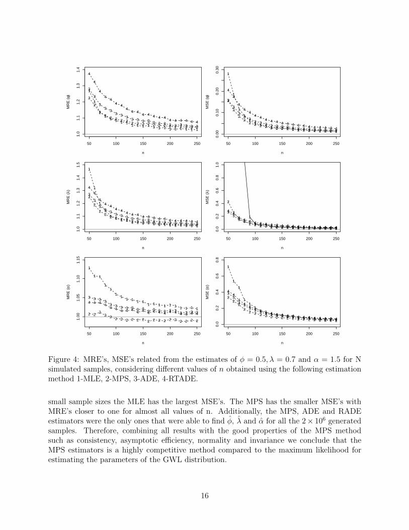
Figure 4: MRE’s, MSE’s related from the estimates of φ = 0.5, λ = 0.7 and α = 1.5 for Nsimulated samples, considering different values of n obtained using the following estimationmethod 1-MLE, 2-MPS, 3-ADE, 4-RTADE.
small sample sizes the MLE has the largest MSE’s. The MPS has the smaller MSE’s withMRE’s closer to one for almost all values of n. Additionally, the MPS, ADE and RADEestimators were the only ones that were able to find φ, λ and α for all the 2× 10⁶ generatedsamples. Therefore, combining all results with the good properties of the MPS methodsuch as consistency, asymptotic efficiency, normality and invariance we conclude that theMPS estimators is a highly competitive method compared to the maximum likelihood forestimating the parameters of the GWL distribution.
16
5 Application
In this section, we compare the GWL distribution fit with several usual three parame-ters lifetime distributions considering two data sets one with bathtub hazard rate andone with the increasing hazard function. For sake of comparison the following lifetimedistributions were considered: The generalized gamma (GG) distribution (Stacy, 1962)with p.d.f given by f(t) = αΓ(φ)−1 βαφ tαφ−1 e−(βt)α , where β > 0, φ > 0 and α > 0,the generalized Weibull (GW) distribution (Mudholkar et al., 1996) with p.d.f given by
f(t) = (αφ)−1(t/φ)1/α−1(1− λ(t/φ)1/α)1/λ−1
, where λ ∈ R the generalized exponential-Poisson (GEP) distribution (Barreto-Souza and Cribatari-Neto, 2009) with p.d.f given by
f(t) =(αβφ/(1− e−φ)
α)e−φ−βt+φ exp(−βt)(1− e−φ+φ exp(−βt))α−1
and the exponentiated
Weibull (EW) distribution (Mudholkar et al., 1995) with p.d.f f(t) = αφβ−1(t/β)α−1×× exp (−(t/β)α) (1− exp (−(t/β)α))
φ−1.
Firstly, it will be considered the TTT-plot (total time on test) in order to verify the be-haviour of the empirical hazard function. Developed by Barlow and Campo (1975) the TTT-plot is achieve through plot of the values [r/n,G(r/n)] whereG(r/n) =
(∑ri=1 ti + (n− r)t(r)
)/∑n
i=1 ti, r = 1, . . . , n, i = 1, . . . , n and t(i) is the order statistics. If the curve is con-cave (convex), the hazard function is increasing (decreasing). When it starts convex andthen concave (concave and then convex) the hazard function will have a bathtub (inversebathtub) shape. Secondly, the discrimination criterion methods are: AIC (Akaike Informa-tion Criteria) and AICc (Corrected Akaike information criterion) computed respectively byAIC = −2l(θ; t) + 2k and AICc = AIC + 2 k (k + 1)(n− k − 1)−1, where k is the num-ber of parameters to be fitted and θ is estimation of θ. Given a set of candidate modelsfor t, the best one provide the minimum values. To check the goodness of fit it will beconsider the Kolmogorov-Smirnov (KS) test . This procedure is based on the KS statisticDn = sup |Fn(t)− F (t;φ, λ, α)|, where sup t is the supremum of the set of distances, Fn(t)is the empirical distribution function and F (t;α, β, λ) is c.d.f. In these case, testing the nullhypothesis that the data comes from F (t;α, β, λ), and with significance level of 5%, we willreject the null hypothesis if the returned p-value is smaller than 0.05.
5.1 Lifetimes data
Presented by Aarset (1987) in table 1 is available the dataset is related to the lifetime inhours of 50 devices put on test
Table 1: Lifetimes data (in hours) related to a device put on test.0.1 0.2 1 1 1 1 1 2 3 6 7 11 1218 18 18 18 18 21 32 36 40 45 46 47 5055 60 63 63 67 67 67 67 72 15 79 82 8283 84 84 84 85 85 85 85 85 86 86
17

Figure 6 shows (left panel) the TTT-plot, (middle panel) the fitted survival superimposedto the empirical survival function and (right panels) the hazard function adjusted by GWLdistribution. Table 9 presents the AIC and AICc criteria and the p-value from the KS testfor all fitted distributions considering the Aarset dataset.
0.0 0.2 0.4 0.6 0.8 1.0
0.0
0.2
0.4
0.6
0.8
1.0
r/n
G(r
/n)
20 40 60 80
0.0
0.2
0.4
0.6
0.8
1.0
Tempos
S(t
)
EmpiricalGen. WLGen. GammaGen. WeibullExp. WeibullGen. EP
0 20 40 60 80
0.00
0.05
0.10
0.15
0.20
0.25
0.30
Tempos
h(t)
Figure 5: (left panel) the TTT-plot, (middle panel) the fitted survival superimposed tothe empirical survival function and (right panels) the hazard function adjusted by GWLdistribution
Table 2: Results of AIC and AICc criteria and the p-value from the KS test for all fitteddistributions considering the Aarset dataset.
Criteria Gen. WL Gen. Gamma Gen. Weibull Exp. Weibull Gen. EPAIC 418.031 448.294 430.055 463.674 486.255AICc 412.552 442.816 424.576 458.196 480.777KS 0.5787 0.0115 0.0453 0.0222 0.0302
Comparing the empirical survival function with the adjusted distributions it can be ob-served a better fit for the GWL distribution among the chosen models. These result isconfirmed from AIC and AICC since GWL distribution has the minimum values and thep-values returned from the KS test are greater than 0.05. Moreover, considering a signifi-cance level of 5%, the others models are not able to fit the proposed data. Table 2 displaysthe MPS estimates, standard errors and the confidence intervals for φ, λ and α of the GWLdistribution.
18

Table 3: MPS estimates, Standard-error and 95% confidence intervals (CI) for φ, λ and α
θ θMPS S.E(θ) CI95%(θ)φ 0.0057 0.00091 ( 0.0039; 0.0075)λ 0.0118 0.00003 (0.0117; 0.0118)α 110.4964 6.58144 (97.5971; 123.3958)
5.2 Average flows data
The study of average flows has been proved of high importance to protect and maintainaquatic resources in streams and rivers (Reiser et al., 1989). In this section, we consider areal data set related to the average flows (m3/s) of the Cantareira system during Januaryat Sao Paulo city in Brazil. Its worth mentioning that the Cantareira system provide waterto 9 million people in the Sao Paulo metropolitan area. The data set available in Table 4was obtained from the website of the National Water Agency including a period from 1930to 2012.
Table 4: January average flows (m3/s) of the Cantareira system.82.0 80.9 102.5 65.3 65.5 47.1 53.0 139.4 82.4 80.2 92.550.0 50.4 50.2 36.2 35.9 100.0 94.2 78.1 54.8 86.9 80.160.3 26.9 48.5 51.0 51.1 84.5 76.9 69.4 77.3 109.2 55.3106.3 30.5 94.2 87.3 115.0 70.0 31.3 87.1 35.9 67.7 55.189.9 50.1 52.6 82.0 54.1 44.3 69.2 94.4 83.4 122.7 88.173.3 35.9 82.4 64.9 90.8 80.4 55.3 31.4 45.7 43.6 45.896.8 85.8 43.6 122.3 66.5 41.0 75.4 79.4 34.8 78.8 52.477.1 47.0 67.4 132.8 144.9 64.1
In this section we consider the ML estimator, showing that both MPS or MLE could beused successfully in applications. Figure 6 shows (left panel) the TTT-plot, (middle panel)the fitted survival superimposed to the empirical survival function and (right panels) thehazard function adjusted by GWL distribution. Table 5 presents the AIC and AICc criteriaand the p-value from the KS test for all fitted distributions considering the data set relatedto the January average flows (m3/s) of the Cantareira system.
Comparing the empirical survival function with the adjusted distributions it can be ob-served a better fit for the GWL distribution among the chosen models. These result isconfirmed from AIC and AICC since GWL distribution has the minimum values and thep-values returned from the KS test are greater than 0.05. Table 6 displays the ML estimates,standard errors and the confidence intervals for φ, λ and α of the GWL distribution.
19

0.0 0.2 0.4 0.6 0.8 1.0
0.0
0.2
0.4
0.6
0.8
1.0
r/n
G(r
/n)
40 60 80 100 120 140
0.0
0.2
0.4
0.6
0.8
1.0
m³ /2
S(t
)
EmpiricalGen. WLGen. GammaGen. WeibullExp. WeibullGen. EP
40 60 80 100 120 140
0.00
0.01
0.02
0.03
0.04
0.05
0.06
m³ /2
h(t)
Figure 6: (left panel) the TTT-plot, (middle panel) the fitted survival superimposed tothe empirical survival function and (right panels) the hazard function adjusted by GWLdistribution
6 Concluding remarks
In this paper, we propose a new lifetime distribution. The GLW distribution is a straight-forwardly generalization of the weighted Lindley distribution proposed by Ghitany et al.(2011), which accommodates increasing, decreasing, decreasing-increasing-decreasing, bath-tub, or unimodal hazard functions, making the GWL distribution a flexible model for re-liability data. The mathematical properties of the new distribution are discussed. It wasalso derived the estimation of the parameters of the GWL distribution using eight estima-tion methods and compared via an intensive simulation study. Most important, from oursimulations we observe that the MLE, ME, LSE, WLSE and the CME estimators fail infinding the parameters estimates for a significant number of samples. The simulations showthat the MPS (maximum product of spacing) is the most efficient method for estimating theparameters of the GWL distribution in comparison with its competitors. Finally, we analyzetwo data sets for illustrative purposes, proving that the GWL outperform several usual threeparameters lifetime distributions.
Appendix
Iφ,φ = −E[∂l(θ; t)
∂φ2
]= − 1
(λ+ φ)2+ ψ′(θ)
20

Table 5: Results of AIC and AICc criteria and the p-value from the KS test for all fitteddistributions considering the data set related to the january average flows (m3/s) of theCantareira system.
Criteria Gen. WL Gen. Gamma Gen. Weibull Exp. Weibull Gen. EPAIC 775.431 775.461 777.280 780.304 778.873AICc 769.735 769.765 771.584 774.608 773.176KS 0.4683 0.4223 0.3935 0.1654 0.4599
Table 6: ML estimates, Standard-error and 95% confidence intervals (CI) for φ, λ and α
θ θMLE S.E(θ) CI95%(θ)φ 7.0485 1.5425 (2.3847; 11.7124)λ 0.1244 0.0557 (0.1183; 0.1305)α 0.9579 0.1173 (0.9310; 0.9849)
Iφ,λ = −E[∂l(θ; t)
∂φ∂λ
]= −α
λ+
1
(λ+ φ)2
Iφ,α = −E[∂l(θ; t)
∂φ∂α
]=−α log(λ)− ψ(φ) + α log(λ)− (λ+ φ)−1
α
Iλ,λ =− E[∂l(θ; t)
∂λ2
]=αφ
λ2+ (α− 1)λα−2(ψ(φ)− α log(λ) + (λ+ φ)−1)
+ E
[αTαλα−2 ((α− 2)λ− (λT )α)
(λ+ (λT )α)
]− 1
(λ+ φ)2
Iα,α =− E[∂l(θ; t)
∂α2
]=φ(λ+ φ+ 1) (ψ(φ)2 + ψ(φ))
α2(λ+ φ)+
1
α2
+2(λ+ 2φ+ 1)ψ(φ) + 2
α2(λ+ φ)− E
[λ(λT )α log(λT )2
(λ+ (λT )α)
]Iα,λ =− E
[∂l(θ; t)
∂α∂λ
]= −φ
λ+λ (1 + φψ(φ)) + φ (1 + (φ+ 1)ψ(φ+ 1))
λ(λ+ φ)
− E[
(1 + αλα−1Tα) (λT )α log(λT )
(λ+ (λT )α)2
]+
(φ+ λ+ 1− 1
α
)Γ(φ+ 1− 1
α
)(λ+ φ)Γ(φ)
− E[
(αλα−1Tα log(λT ) + (λT )α−1)
(λ+ (λT )α)
]
21

References
[1] AARSET, M.V. How to identify a bathtub hazard rate, IEEE Transactions Reliability,36, p.106-108, 1987.
[2] AKAIKE, H. 1974. A new look at the statistical model identification. IEEE Transactionson Automatic Control, 19(6): 716-723.
[3] Al-MUTAIRI, D. K., GHITANY, M. E., KUNDU, D. Inferences on stress-strength reli-ability from weighted Lindley distributions. Communications in Statistics - Theory andMethods, v. 44, 19, 2015.
[4] ALI, S. On the Bayesian estimation of the weighted Lindley distribution, Journal ofStatistical Computation and Simulation, p.1-26, 2013.
[5] BAKOUCH, H.S., AL-ZAHRANI, B.M., AL-SHOMRANI, A.A., MARCHI, V.A.A.,LOUZADA, F. An extended Lindley distribution. Journal of the Korean Statistical So-ciety, 41, 75-85. 2012.
[6] BARLOW, R. E.;CAMPO, R. A. Total Time on Test processes and applications to failuredata analysis. In Reliability and fault tree analysis. SIAM, Pennsylvania, 1975.
[7] BARRETO-SOUZA, W. and BAKOUCH, H.S. A new lifetime model with decreasingfailure rate. Statistics, 47, 465-476. 2013.
[8] BARRETO-SOUZA. W., CRIBARI-NETO,F. A generalization of the exponential-poisson distribution, Statist. Probab. Lett. 79, 2493-2500. 2009.
[9] BONFERRONI C.E. Elmenti di statistica generale. Libreria Seber, Firenze. 1930.
[10] CASELLA, G.; BERGER, R. Statistical Inference (2nd ed.), Belmont, CA: Duxbury,2002.
[11] CHENG, R.C.H., AMIN, N.A.K. Maximum product of spacings estimation with appli-cation to the lognormal distributions. Math Report 79-1, Department of Mathematics,UWIST, Cardiff. 1979.
[12] CHENG, R.C.H., AMIN, N.A.K. Estimating parameters in continuous univariate dis-tributions with a shifted origin. J. Roy. Statist. Soc. Ser. B 45, 394-403. 1983.
[13] CHENG, R.C.H; STEPHENS, M. A. A goodness-of-fit test using Morans statistic withestimated parameters. Biometrika 76 (2): 386392. 1989.
[14] D’AGOSTINO, R. STEPHENS, M. Goodness-of-fit techniques. Marcel Dekker, Inc.,New York. 1986.
22

[15] GHITANY, M.E; ALQALLAF, F; AL-MUTAIRI, D.K; HUSAIN, H.A. A two-parameterweighted Lindley distribution and its applications to survival data, Mathematics andComputers in Simulation 81 11901201, 2011.
[16] GHITANY, M.E., Al-MUTAIRI, D.K., BALAKRISHNAN, N. and Al-ENEZI, L.J.Power Lindley distribution and associated inference. Computational Statistics and DataAnalysis, 64, 20-33, 2013.
[17] GHITANY, M.E; ATIEH, B; NADARAJAH, S. Lindley distribution and its application,Mathematics and Computers in Simulation, 78(4), 493506, 2008.
[18] GLASER, R.E. Bathtub and related failure rate characterization. J. Amer. StatisticalAssoc, v. 75, p. 667-672, 1980.
[19] LAWLESS, J. F. Statistical models and methods for lifetime data, Second Edition, NewYork: John Wiley and Sons, 664 p, 2002.
[20] LUCENO, A Fitting the Generalized Pareto Distribution to Data using MaximumGoodness-of-fit Estimators. Computational Statistics and Data Analysis, 51(2), 904-917.2006.
[21] MACDONALD, P.D.M. An estimation procedure for mixtures of distribution. J. Roy.Statist. Soc. Ser. B, 33, 326-329. 1971.
[22] MAZUCHELI, J; LOUZADA, F; GHITANY, M.E. Comparison of estimation meth-ods for the parameters of the weighted Lindley distribution, Applied Mathematics andComputation, 220(1) , 463471, 2013.
[23] MUDHOLKAR, G. S., SRIVASTAVA, D. K., FREIMER, M. The exponentiated Weibullfamily: a reanalysis of the bus-motor-failure data. Technometrics, 37(4), 436-445, 1995.
[24] MUDHOLKAR, G. S., SRIVASTAVA, D. K., KOLLIA, G. D. A generalization of theWeibull distribution with application to the analysis of survival data. Journal of theAmerican Statistical Association, 91(436), 1575-1583, 1996.
[25] POPESCU, T.D., AIORDACHIOAIE, D. Signal segmentation in time-frequency planeusing Renyi entropy - Application in seismic signal processing. In: Proceedings of theSecond International Conference on Control and Fault-Tolerant Systems, pp. 312-317,2013.
[26] RANNEBY, B. The maximum spacing method: An estimation method related to themaximum likelihood method. Scandinavian Journal of Statistics 11, 93-112, 1984.
[27] RENYI, A. On measures of entropy and information. In: Proceedings of the 4th BerkeleySymposium on Mathematical Statistics and Probability, volume I, pp. 547-561. Universityof California Press, Berkeley, 1961.
23

[28] R CORE TEAM. R: A language and environment for statistical computing. R Founda-tion for Statistical Computing, Vienna, Austria, 2014.
[29] STACY, E. W. A generalization of the gamma distribution. Annals of MathematicalStatistics, 28: 1187-1192, 1962.
[30] STEPHENS, M.A. EDF statistics for goodness of fit and some comparisons J. Amer.Stat. Assoc., 69, 730-737, 1974.
[31] SHANNON, C. E. A Mathematical theory of communication. Bell System TechnicalJournal, v.27, p 623-659, 1948.
[32] WANG, W. Bias-corrected maximum likelihood estimation of the parameters of theWeighted Lindley distribution, Master’s report, Michigan Technological University, 62p,2015.
[33] ZALERZADEH, H., DOLATI, A. Generalized Lindley distribution. Journal of Mathe-matical Extension. 2009. 3, 13-25.
24