Acta Genet Med Gemellol 28:197-210 (1979) The Mendel Institute/Alan R. Uss, Inc.

Received 11 April 1979 Final 3 October 1979

The Genetical Relationship of Impulsiveness and Sensation Seeking to Eysenck's Personality Dimensions

N. G. Martin 1 I L. J. Eaves l

I D. W. Fulker2

1 Department of Genetics, University of Birmingham; 2 Department of Psychology, Institute of Psychiatry, London

The genetical analysis of covariance structures is used to explore the genetical and environ­mental intercorrelations of impulsiveness and sensation seeking factors and their conform­ity to Eysenck's principal personality dimensions. The independent dimensions of psycho­ticism, extraversion, neuroticism, and lie scale are not found to give a very satisfactory account of the genetical factor structure. In particular, it is clear that impulsiveness and sensation seeking are not simple reflections of extraversion.

Key words: Genetic analysis, Covariance structures, Impulsiveness, Sensation seeking, Extraversion, Eysenck Personality Questionnaire, Twin study

INTRODUCTION

For many years Eysenck [8] has argued that the main features of individual differences in personality can be explained with reference to three independent high-order factors: psychoticism (P), extraversion (E), and neuroticism (N). These three factors are always extracted from administrations of the Eysenck Personality Questionnaire (EPQ) (and simi­lar ones are extracted from other personality scales), along with a further factor - the lie scale (L), which seems to be a measure of dissimulation or social desirability but whose significance is less clear than the three major factors. Some authors have considered that this scheme is too coarse-grained and ignores many facets of personality that really pro­vide the interesting contrasts between people. Thus Guildford [13] concluded that E was a kind of "shotgun wedding" between rhathymia (akin to impulsiveness) and soci­ability. Eaves and Eysenck [3] tested 837 twin pairs with scales of sociability and im­pulsiveness and showed, indeed, that the subjects X scales interaction had a significant genetical component suggesting "some justification for regarding Sociability and Im­pUlsiveness as distinguishable genetically". However, they estimated the genetical corre-

L.J. Eaves' present address: Department of Experimental Psychology, University of Oxford, UK.

0001-5660/79/2803-0197$02.60 © 1979 Alan R. Liss, Inc.

198 Martin, Eaves, and Fulker

lation between the two as 0.42 and the environmental correlation to be 0.66, supporting Eaves' earlier view [2] that the unitary nature of extraversion is due more to enivronmental than to genetical influences.

Various authors have suggested that impulsiveness itself is a combination of subfactors tha t would more usefully be considered separately. Eysenck and Eysenck [9] have factor analysed a set of items related to impulsiveness (in the broad sense) into four primary factors, which they call impulsiveness in the narrow sense (IMPN), risk taking (RISK), non­planning (NONP), and liveliness (LIVE), and have related these to P, E, N, and L. Eaves et al [7] estimated the common factor and specific components of the variation in these four traits and showed that the same factor structure was operating for both genetical and environmental sources of variation.

Zuckerman [24] has demonstrated that sensation seeking is an important aspect of personality through which the individual regulates his degree of arousal. Consequently one would expect it to be related to extraversion, which is thought to vary with the same physiological function [8] . However, Eysenck and Zuckerman [10] have shown that the four subscales of sensation seeking have different phenotypic correlations with P, E, N, and L. These four sub factors are Disinhibition (DIS), thrill and adventure seeking (T AS), ex~ perience seeking (ES), and boredom susceptibility (BS), and the genetical and e~viron­mental covariance among these four factors has been explored by Fulker et al [12].

The present paper takes advantage of the fact that scores for the four impulsiveness factors, the four sensation seeking factors and P, E, N, and L were obtained for samples from the Maudsley Twin Register in 1975. This provides the opportunity to examine the genetical and environmental causes of covariation among the 12 variables using the genetic­al analysis of covariance structures approach of Martin and Eaves [19] .

The genetical analysis of covariance structures, based on the work of Joreskog [15] , allows the research worker to test models of co variation incorporating various genetical and environmental sources of covariation and different factor structures through which these sources influence the traits in question. In our case, with 12 variables, there are many models one might fit to the data, including a great variety of empirical factor structures. This approach risks the accusation of "looking for a model that fits", so we shall restrict our hypotheses to those that attempt to relate the covariation among the eight factors of impulsiveness and sensation seeking to Eysenck's four principal dimensions of personality, P, E, N, and L.

THE DATA

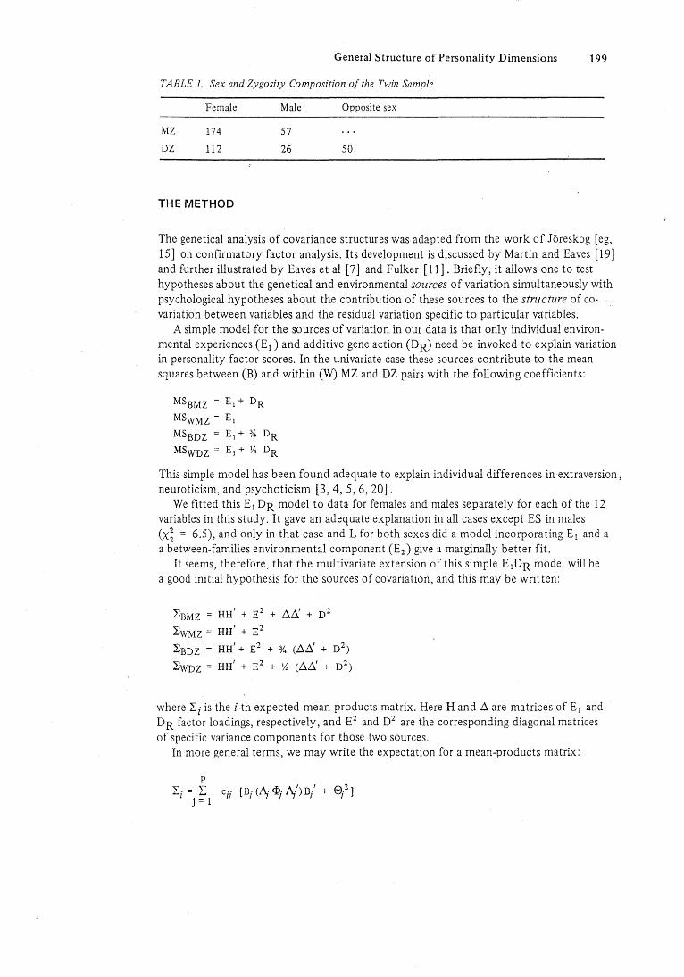
The three self-report questionnaires were sent by post to twins from the Maudsley Twin Register during 1975, the impulsiveness questionnaire and EPQ together, and the sensation seeking questionnaire (SSQ) on a separate occasion. Details of the impulsiveness and EPQ scales are given by Eysenck and Eysenck [9] and Eaves et al [7] ; those of the sensation seeking questionnaire, by Fulker et a1 [12]. The number of items in each is: IMPN (12), RISK (10), NONP (12), LIVE (6), P (25), E (21), N (23), L (21), DIS (10), TAS (10), ES (10), and BS (10). Whereas 588 pairs replied to the first two questionnaires, only 441 pairs replied to the SSQ, leaving an intersect of 438 pairs whose sex and zygosity distribution is shown in Table 1. Zygosity determination in the Maudsley Twin Register is discussed by Kasriel and Eaves [17] . The age range of respondents was 16 to 73 years, with a mean of 31 years.

An angular transformation was applied to the raw scores for each factor to improve the additive pro­perties of the scales. Between- and within-mean products matrices were calculated for all five twin groups, providing ten matrices in all. The between-mean products matrices were corrected for linear regression in age, so reducing their degrees of freedom by one. The within-mean products matrix for DZ opposite-sex pairs was corrected for the mean difference between males and females, thus reducing its degrees of free­dom by one. The ten 12 X 12 matrices, corrected for age and sex, are reproduced in the Appendix.

General Structure of Personality Dimensions 199

TABLE 1. Sex and Zygosity Composition of the Twin Sample

MZ

DZ

Female

174

112

THE METHOD

Male

57

26

Opposite sex

50

The genetical analysis of covariance structures was adapted from the work of Joreskog [eg, 15] on confirmatory factor analysis. Its development is discussed by Martin and Eaves [19] and further illustrated by Eaves et al [7] and Fulker [11] . Briefly, it allows one to test hypotheses about the genetical and environmental sources of variation simultaneously with psychological hypotheses about the contribution of these sources to the structure of co­variation between variables and the residual variation specific to particular variables.

A simple model for the sources of variation in our data is that only individual environ­mental experiences (E 1 ) and additive gene action (DR) need be invoked to explain variation in personality factor scores. In the univariate case these sources contribute to the mean squares between (B) and within (W) MZ and DZ pairs with the following coefficients:

MSBMZ = E) + DR

MSWMZ = £)

MSBDZ = MSWDZ =

This simple model has been found adequate to explain individual differences in extraversion, neuroticism, and psychoticism [3,4,5,6,20].

We fitted this E1 DR model to data for females and males separately for each of the 12 variables in this study, It gave an adequate explanation in all cases except ES in males (X; = 6.5), and only in that case and L for both sexes did a model incorporating Eland a a between-families environmental component (E2 ) give a marginally better fit.

lt seems, therefore, that the multivariate extension of this simple E1DR model will be a good initial hypothesis for the sources of covariation, and this may be written:

~BMZ = HH' + £2 + !:It::. + D2

~WMZ = HH' + E2

~BDZ = HH' + £2 + % (!:It::. + D2)

~WDZ = HH' + E2 + ~ (!:It::. + D2)

where ~i is the i-th expected mean products matrix. Here Hand !:l are matrices of E1 and DR factor loadings, respectively, and E2 and D2 are the corresponding diagonal matrices of specific variance components for those two sources.

In more general terms, we may write the expectation for a mean-products matrLx:

p }:. = I: c·· [B, (A. <p. A·')B·' + 8.2 J

I j = 1 IJ J' 7 J' 7 J J

200 Martin, Eaves, and Fulker

where there are p sources of variation and Cij is the coefficient from the univariate model for the i-th mean square and j-th source. For the j-th source t:.j is the matrix of factor load­ings and e/ the diagonal matrix of specific variance components, as above. Note, however, that we may complicate the model by introducing correlations between the factors in iJ!j' or relate the factor structures of different sources by a simple scalar held in the diagonal matrix B. We shall not employ these facilities much in this example.

Having specified the sources of variation and the factor structures of our model, how do we go about testing it? The approach is described fully by Martin and Eaves [19] . Generally, our dat'a will consist of k matrices of mean products. We may write Si for the ith matrix, having Ni degrees of freedom. Given some model for the Si' we may compute the expected values L,i, being positive definite, for particular values of the parameters of the model. When the observations are multivariate normal, we may write the log likeli­hood of obtaining the k observed independent Si as:

i = k log 1 = -¥2 1: Ni [log \' L,i I + tr (St' Li -1) 1

i= 1

(omitting the constant term). For a given model we require the parameter estimates that maximise log L. ,Given maxi­

mum-likelihood estimates of our parameters, we may test the hypothesis that a less re­stricting model (ie, one involving more parameters) does not significantly improve the fit by computing:

X2 2(lo -lI),

where L 1 is the log likelihood obtained under the restricted hypothesis (HI) and Lo is the log likelihood obtained under the less demanding hypothesis (Ho). The Ho we shall adopt in practice is that which assumes that as many parameters are required to explain the data as there are independent mean squares and mean products in the first place; ie, L i = S i for every i. In this case we have simply:

i= k

Lo = - 12 1: N i [ log lSi I + p] i = 1

When we have k matrices the X2 has 12kp (p + 1) -m df, where m denotes the number of parameters estimated under HI and p is the number of variables.

The likelihood is maximised by attempting to minimise -log L for a given model. There are many numerical methods for doing this. A variety of these methods has been implemented by the Numerical Algorithms Group (1974), and we employed the most flexible of their FOR­TRAN routines, E04HAF, for constrained minimisation. The routine has the advantage of allowing the user certain flexibility in the choiCe of method. In particular, minimisation can be based on evaluation of the function values alone (in this case the values of -log Land any functions used in specifying constraints on parameter values), or minimisation can be assisted by computation of first derivatives or of first and second derivatives of the function. Furthermore, differentiation can proceed numerically or can be programmed precisely by the user. For our problem the Powell 64 method was used, which relies only on the evalu­ation of the functions themselves, since coding the first derivatives was tedious, and their approximate routine was used because of the need to ensure the 'I,i are all positive defmite. For our simple example these constraints should be automatically satisfied, providing we estimate D and E rather than D2 and E2. The problem thus reduces to an unconstrained problem in our case. However, in problems that are factorially more complex, further

General Structure of Personality Dimensions 201

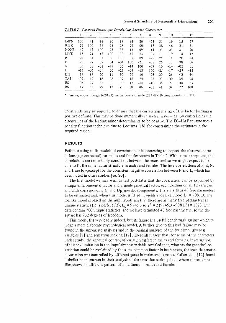
TABLE 2. Observed Phenotypic Correlations Between Characters*

2 3 4 5 6 7 8 9 10 11 12

IMPN 100 41 36 30 34 36 20 -23 31 19 15 27 RISK 36 100 37 24 28 29 00 -13 38 46 21 31 NONP 40 43 100 23 33 17 -09 -14 23 23 31 20 LIVE 18 21 13 100 03 42 -23 -07 17 19 14 12 P 24 34 31 00 100 07 09 -29 25 11 20 24 E ")fI 27 fI'7 34 -04 100 ")1 flO 26 1'7 08 1t:. kV VI -"'..l -vu ..ll ..lV

N 33 08 -01 -22 06 -14 100 -07 10 -14 -03 01 L -15 -07 -09 00 -25 -04 -13 100 -25 -17 -27 -13 DIS 17 37 20 11 30 29 10 -26 100 26 42 44 TAS -02 42 16 08 09 16 -24 -05 23 100 39 18 ES 05 27 35 02 30 12 -10 -10 36 27 100 23 BS 17 33 29 12 29 10 06 -01 41 04 22 100

*Females, upper triangle (620 df); males, lower triangle (214 df). Decimal points omitted.

constraints may be required to ensure that the correlation matrix of the factor loadings is positive definite. This may be done numerically in several ways - eg, by constraining the eigenvalues of the leading minor determinants to be positive. The E04HAF routine uses a penalty function technique due to Lootsma [18] for constraining the estimates in the required region.

RESULTS

Before starting to fit models of covariation, it is interesting to inspect the observed corre­lations (age corrected) for males and females shown in Table 2. With some exceptions, the correlations are remarkably consistent between the sexes, and so we might expect to be able to fit the same factor structure in males and females. The intercorrelations of P, E, N) and L are low,except for the consistent negative correlation between P and L, which has been noted in other studies [eg, 20] .

The first model we may wish to test postulates that the covariation can be explained by a single environmental factor and a single genetical factor, each loading on all 12 variables and with corresponding E1 and DR specific components. There are thus 48 free parameters to be estimated and, when this model is fitted, it yields a log likelihood L1 = 9081.3. The log likelihood is based on the null hypothesis that there are as many free parameters as unique statistics (ie, a perfect fit), Lo = 9745.3 so X

2 = 2 (9745.3 -9081.3) = 1328. Our data contain 780 unique statistics, and we have ,estimated 48 free parameters, so the chi­square has 732 degrees of freedom.

This model fits very badly indeed, but its failure is a useful benchmark against which to judge a more elaborate psychological model. A further clue to this bad failure may be found in the univariate analyses and in the original analyses of the four impulsiveness variables [7] and sensation seeking [12] . These all suggest that, for some of the characters under study, the genetical control of variation differs in males and females. Investigation of this sex limitation in the impulsiveness variable revealed that, whereas the genetical co­variation could be explained by the same common factor in both sexes, the specific genetic­al variation was controlled by different genes in males and females. Fulker et al [12] found a similar phenomenon in their analysis of the sensation seeking data, where subscale pro­files showed a different pattern of inheritance in males and females.

202 Martin, Eaves, and Fulker

Clearly, we must take account of this sex limitation in our model, and we do it by esti­mating separate di's fer males and females. The model is that described above, except that we have slightly different expectations for the opposite-sex (OS) pairs, as follows:

~BOS = % .1.1' + ~ (Dm2 + Df2

) + HH' + E2

LWPS = ~ .1S+ ~(Dm2 + Df2) + HH'+ E2

Dm 2 and Df2 denote the specific additive genetical variances for males and females, re­spectively. In the expectations for like-sex pairs we merely substitute Dm 2 for D2 in the males and Df2 for D2 in the female pairs.

The psychological model we wish to test is that the genetical and environmental co­variation between the 12 personality variables can be adequately explained within the framework of Eysenck's four principal dimensions. We therefore define four factors, one each for P, E, N, and L, and allow the eight impulsiveness and sensation seeking variables to load on them. Although experience and the data suggest that we should allow the P and L factors to be correlated, for the sake of simplicity we shall make the four factors ortho­gonal (ie, we fix <I> as an identity matrix). We shall expect the four genetical fac,tors to account for all the genetical variation and covariation of P, E, N, and L, respectively, and so we shall not allow any specific genetic variance components for these four pivotal variables. We expect, however, specific environmental variation for all variables, if only because of measurement error.

Our model thus consists of four orthogonal El factors, each loading on nine variables (four impulsiveness, four sensation seeking, plus the "s'!perfactor"), four DR factors in the same structu:e, 12 El specific standard deviations (eD, and eight DR specific standard deviations (the e i for P, E, N, and L are fixed to zero) each for males and females. Thus, there is a total of 100 (36 + 36 + 12 + 8 + 8) free parameters to be estimated.

Not surprisingly, this maximisation consumes a lot of computer time, but the log likeli­hood finally converged on is L 1 = 9263.8. The likelihood ratio test for goodness-of-fit of the model gives X2

680 = 963, still a very poor fit but a great improvement (X2 52 = 365) on the first model.

The maximum-likelihood estimates of the parameters are shown in Table 3. Ideally, we should like to attach standard errors to these estimates and perhaps discard the nonsignifi­cant ones before refitting the modeL Martin and Eaves [19] show how the covariance matrix of the estimates may be evaluated, but in this example with 100 parameters the evaluation took too long, even with the extensive computer resources at our disposal.

If the stringent application of Eysenck's superfactor model produces such a poor fit, we may ask whether a better fit can be obtaineCl by relaxing some of the constraints of the model. If we allow P, E, N, and L to have specific genetical components (different for males and females) so that the superfactors are not required to account for all the variation and covariation in these four variables, the addition of these eight free para­meters gives a fit of X2 p72 = 878 or an improvement of X~ = 85 over the more stringent model.

If the factor structures for environmental and genetical sources of variation are very similar, it may be possible to improve the fit of the model by constraining the Eland DR factor loadings to be related by a single constant, b (which will be related to the heritabil­ity of the common factors). This was done successfully for the impulsiveness data alone by Eaves et al [7] . This modification was made to the less stringent model resulting in a saving of 35 parameters (-36 + 1), but this 73-parameter model gave an even worse fit, X~07 = 1057, or a deterioration of X~5 = 179.

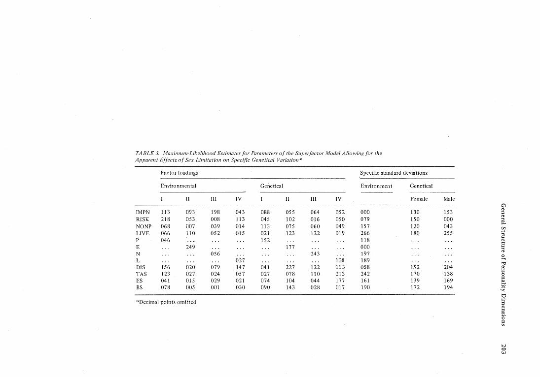
TABLE 3. Maximum-Likelihood Estimates for Parameters of the Superfactor Model Allowing for the Apparent Effects of Sex Limitation on Specific Genetical Variation*

Factor loadings Specific standard deviations

Environmental Genetical Environment Genetical

II III IV I II III IV Female Male CJ

IMPN 113 093 198 043 088 055 064 052 000 130 153 (D

::: RISK 218 053 008 113 045 102 016 050 079 150 000

(D >-t

NONP 068 007 039 014 113 075 060 049 157 120 043 e. C/l

LIVE 066 110 052 015 021 123 122 019 266 180 255 ...... >-t

P 046 152 118 s:: (")

E 249 177 000 a >-t

N 056 243 197 (D

0

L 027 138 189 ......, "'t:'

DIS 156 020 079 147 041 227 122 113 058 152 204 (D >-t

TAS 123 027 024 057 027 078 110 213 242 170 138 en 0

ES 041 015 029 021 074 104 044 177 161 139 169 ::: ~

BS 078 005 001 030 090 143 028 017 190 172 194 ...... '< t:1

*Decimal points omitted S' (D

::: en 0' ::: en

t-.> 0 w

204 Martin, Eaves, and Fulker

It is ~pparent that other factor structures may give a better account of the data, but none of the models tried went anywhere near an acceptable level of significance. This seems to be a problem frequently encountered but little discussed by those who work with maxi­mum likelihood factor analysis and analysis of covariance structures. The trouble seems to be that one obtains a very sensitive test of the model, which may fail from all sorts of trivial departures not related to the hypothesis under test. Of course, the significance level is directly related to sample size, but it does seem to be common experience among workers in this area that it is often impossible to get any but the most overspecified model to fit [1, 14J

How, then, is one to judge when to stop fitting extra parameters when all such models fail on the likelihood ratio criterion? Joreskog [16] advocates use of Tucker and Lewis' reliability coefficient [23] as a guide to the proportion of total dispersion accounted for by the model.

For our case with several matrices we may modify their argument and the computation of the reliability coefficient, p, as follows. For a given model, X2 n gives the likelihood ratio criterion for goodness-of-fit. This X2nl n is Fn, 00, and if the model fits, the expected value of F is 1, so for a particular case F -1 is a measure of goodness-of-fit of the model. If we now compute Fo for a "stupid" model, Ho (eg, no factors, no genetical variation), a~d Fi under a particular "sensible" model, Hi, then Fo-FI is a measure of "improvement" due to HI' The "total improvement possible" is Fo-l, so the reliability coefficient

= FO-Fj p Fo -j

is the proportional improvement achieved by our model H j • This is the same as Tucker and Lewis' coefficient, except that they apply a correction to improve the approximation to X2.

The most inappropriate model imaginable for our data might consist of only 12 E 1

specific standard deviations. No covariation is allowed for between variables, nor is any additive genetic variation specified to account for different MZ and DZ intrapair corre­lations. When this 12-parameter model is fitted it yields a X;68 = 3312. Judged against this, the 48-parameter model first tested has a reliability coefficient of 0.75, the 1 DO-para­meter "superfactor" model has p = 0.87, and the less stringent 108-parameter model has p = a .91. A coefficient of 0.95 has been suggested as an acceptable reliability for a model, and by this criterion the laO-parameter "superfactor" is inadequate.

Another criterion that may assist decision-making in this type of model fitting is Akaike's Information Criterion [see, eg, 22] AIC = 2Ll + 2m (m free parameters), which balances an increase in likelihood with the loss of parsimony involved in fitting the extra parameters to achieve this. Akaike suggests that the model with minimum AIC is the most desirable, and by this criterion we should still choose the relaxed superfactor model of 108 parameters. However, the object of this paper is to examine" the conformity of the pattern of environ­mental and genetical covariation between the impulsiveness and sensation seeking variables with Eysenck's scheme of the principal personality dimensions, and we shall restrict our discussion to this model.

DISCUSSION

Several criteria suggest that the "superfactor" model for genetical and environmental co­variation between the 12 personality variables shown in Table 3 is wanting. However, let us judge the seriousness of this inadequacy by closer inspection of the results.

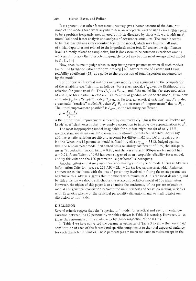
In Table 4 we have converted the parameter estimates of Table 3 to show the percentage contribution of each of the factors and specific components to the total expected variance for each character in females. These percentages are much the same in males except in the

TABLE 4. Percentage Contributions of Individual Environmental (E 1) and Additive Genetic (DR) Factor and Specific Components to Total Variation for Each Character in Females

Individual environments (E1) Additive genes (V2 DR) Total expected

II III IV Specific (Error)a I (P) II (E) III (N) IV (L) Specific variance

IMPN 16 11 49 2 0 (26) 5 2 3 2 10 0.0797 c;'1 RISK 54 3 0 15 7 (28) 1 6 0 13 0.0884

(1:l

:::: NONP 9 0 3 0 49 (41) 13 6 4 2 14 0.0504

(1:l >-t

LIVE 4 10 2 0 58 (34) 0 6 6 0 14 0.1218 ~ (/)

P 8 50 (36) 42 0.0274 ...... >-t

E -80 0 (15) 20 0.0775 ~ 0 ......

N 4 54 (15) 42 0.0715 ~ >-t

L 2 78 (26) 20 0.0458 (1:l

0 DIS 23 0 6 20 3 (23) 1 24 7 6 10 0.1079 .....,

TAS 12 1 0 3 47 (20) 0 2 5 18 12 0.1248 ~ (1:l >-t

ES 3 0 1 41 (39) 4 8 2 25 15 0.0634 til 0

BS 8 0 0 50 (34) 6 14 0 20 0.0727 :::: ~ ...... '<

aExpected measurement error is calculated as 1,4n. t:1 S' (1:l

:::: til o· :::: til

~ 0 Ul

206 Martin, Eaves, and Fulker

specific genetical contributions for risk (0%), nonplanning (2%), liveliness (24%), and disinhib~ ition (18%). One possible explanation for different specific genetic contributions to variance in males and females is the very different degree of selection for the male and the female twins (83 vs 286 same-sexed pairs), and one wonders if some of the apparent male-female differences might stem from this source.

It is clear that most of the El variance is specific to each variable and that the "factors" are largely artificial, most loading substantially on only one variable. Thus, factor II takes out all the E 1 variance for E, III for IMPN, and I for RISK. The E 1 variance for DIS is divided equally between factors I and IV, and it is only factor I that has anything like the appearance of a genuine El common factor. Since El variance is, ofits nature, specific, it is not surprising to find that this is an unimportant source of covariation.

Such covariation as there is appears more likely to be explained by the four genetical superfactors that have been forced to assume the dimensions of P, E, N, and L. The sum of components due to genetic factors and specific genes for anyone variable is the herit­ability for that variable and it can be seen that most of these are rather low. Nevertheless, for all variables except RISK, over half the variation is due to common factors.

The genetical P factor accounts for much of the covariation with non-planning, whereas the E factor loads heavily on disinhibition and boredom susceptibility. The N factor appears to account for little of the genetical covariation between variables, but L, or social desirabil­ity, appears to be genetically related (inversely) to thrill and adventure seeking and exper­ience seeking.

Because the raw data were subjected to an angular transformation each variable has an expected measurement error variance equal to ~n (where the scale has n items), pro­vided the items are all of equal difficulty. If the items of a scale are not equally difficult, then this estimate of error will be larger than the true value. These expected measurement errors, expressed as a percentage of the expected total variation for each variable, are shown in Table 4 under the column marked "Error". It can be seen that in many cases error accounts for a substantial part of the specific (or quasi-specific) El variation. Correc­tion of "heritabilities" for this source of measurement error will increase the heritability of the reliable variance, substantially in some cases.

Although we are not particularly satisfied with the model we have set out to test, another way of viewing its adequacy is to inspect the residuals left after subtracting the predicted correlations for those observed. To do this for all ten 12 X 12 matrices is more than the mind can absorb, but inspe ction of the single phenotypic correlation matrix will give us some guide. The residual phenotypic correlation matrices for males and females are

shown in Table 5, and most of the deviations are quite respectably small. Of the larger de­viations, many if not most can be seen to involve the L factor, which suggests that we have not satisfactorily incorporated this variable in our factor structure. On the other hand, a possible clue to this anomaly may lie in the biggest deviation of Table 5, which is for the P-L correlation. Our model failed to take account of this well-known correlation, and forcing these two factors to be orthogonal may have been deterimental to the model.

However, the fundamental hypothesis we set out to test, that covariation between im­pulsiveness and sensation seeking variables would be largely explicable in terms of the E factor, has received only limited support. The P and L factors seem equally important, but it is also apparent that the attempt to fit these variables within the straightjacket of P, E, N, and L, is far from satisfactory.

Whatever the substantive findings of this paper, the work illustrates the value of the method in allowing us to combine the testing of structural psychological hypotheses with

General Structure of Personality Dimensions 207

TABLE 5. Residual Phenotypic Correlations (Observed-Expected) *

2 3 4 5 6 7 8 9 10 11 12

IMPN 02 02 02 09 00 -05 -15 04 07 05 02 RISK -05 01 01 01 02 -03 -12 03 06 -01 02 NONP 04- 01 05 02 03 00 -08 02 00 05 -04 LIVE -OS -03 -06 01 02 -10 -05 02 00 03 00 P -01 05 -03 -02 07 09 -29 06 05 02 01 E -15 -02 -07 -04 -04 -21 -OS -01 03 00 01 N 08 05 08 -10 06 -14 -07 -02 01 08 -03 L -07 -06 -03 03 -25 -04 -13 -08 01 -04 -09 DIS -OS 01 -01 -03 11 03 -01 -09 03 03 02 TAS -15 -02 -09 -10 03 03 -OS 13 00 07 05 ES -05 04 OS -OS 13 04 00 13 00 -04 01 BS -07 02 04 01 07 -05 01 02 01 -09 01

*Females, Upper Triangle; Males, Lower Triangle. Decimal points omitted.

a variety of genetical and environmental models of covariation. The scientific advantage of this approach over the all too common practice of "look and see" cannot be' overemphas­ised.

Acknowledgments. We should like to thank Professor H. J. Eysenck for his comments on the manu­script and Professor M. Zuckerman and Dr. S. B. G. Eysenck for permission to use their data collected for the Maudsley Twin Register by Mrs. J. Kasriel. The extensive computations were carried out on the CDC 7600 at University of Manchester Regional Computing Centre. N. G. M. and 1. J. E. were supported by an M. R. C. programme grant in psychogenetics.

REFERENCES

1. Duncan-Jones P (1980): The structure of social relationships: analysis of a survey instrument. Soc Psychiat (in press).

2. Eaves LJ (1973): The structure of genotypic and environmental covariation for personality measurements: An analysis of the PEN. Br J Soc Clin PsycholI2:275-282.

3. Eaves LJ, Eysenck HJ (1975): The nature of extraversion: A genetical analysis. J Pers Soc PsychoI32:102-1l2.

4. Eaves LJ, Eysenck Hl (1976): Genetic and environmental components of inconsistency and un­repeatability in twins' responses to a neuroticism questionnaire. Behav Genet 6:145-160.

5. Eaves LJ, Eysenck HJ (1977): A genotype-environmental model for psychoticism. Adv Behav Res Ther 1 :5-26.

6. Eaves LJ, Last KA, Young PA, Martin NG (1978): Model-fitting approaches to the analysis of human behaviour. Heredity 41 :249-320. .

7. Eaves LJ, Martin NG, Eysenck SBG (1977): An application of the analysis of covariance structures to the psychogenetical study of impulsiveness. Br J Math Statist Psycho130:185-197.

S. Eysenck HJ (1967): "The Biological Basis of Personality." Springfield, Illinois: Charles C Thomas. 9. Eysenck SBG, and Eysenck HJ (1977): The place of impulsiveness in a dimensional system of

personality description. Br J Soc Clin Psychol16:57-68. 10. Eysenck SBG, Zuckerman M (1978): Relationship between sensation seeking and Eysenck's

dimensions of personality. Br J Psychol 69:483-4S8. 11. Fulker DW (1978): Multivariate extensions ofa biometrical model of twin data. "Proceedings

of the Second International Congress on Twin Studies, 1978." New York: Alan R. Liss. 12. Fulker DW, Zuckerman M, Eysenck SBG (1979): A genetic and environmental analysis of

sensation seeking. J Res Personality (in press). 13. Guilford lP (1975): Factors and factors of personality. Psychol Bu1182:S02-814.

208 Martin, Eaves, and Fulker

14. Joreskog KG (1969): A general approL.;h to confirmatory maximum likelihood factor analysis. Psychometrika 34:183-202.

15. Joreskog KJ (1973): Analysis of covariance structures. In Krishnaiah PR (ed): "Multivariate Analysis III. Proceedings of the Third International Symposium on Multivariate Analysis." New York: Academic Press.

16. Joresko~ KJ (1976): Factor analysis by least-squares and maximum likelihood methods. In Enstein 'K, Ralston A, Wilf (eds): "Statistical Methods for Digital Computers." New York: Wiley.

17. Kasriel J, Eaves LJ (1976): The zygosity of twins: Further evidence on the agreement between dia­gnosis by blood groups and written questionnaires. J Biosoc Sci 8:263-266.

18. Lootsma FA (1972): A survey of methods for solving constrained minimization problems via un­constrained minimization. In Lootsma FA (ed): "Numerical Methods for Non-linear Optimization." New York: Academic Press.

19. Martin NG, Eaves LJ (1977): The genetical analysis of covariance structure. Heredity 38:77-95. 20. Martin NG, Eysenck HJ (1976): Genetic factors in sexual behaviour. In Eysenck HJ (ed):

"Sex and Personality." London: Open Books. 21. Numerical Algorithms Group (1974): E04HAF. In NAG Library Mark 5 Manual: Oxford University:

NAG Central Office. 22. Ozaki T (1977): On the order determination of ARIMA models. Appl Statist 26:290-30l. 23. Tucker LR, Lewis C (1973): A reliability coefficient for maximum likelihood factor analysis.

Psychometrika 38: 1-1 O. 24. Zuckerman M (1974): The sensation Seeking motive. In Maher B.(ed): "Progress in Experimental

Personality Research," Vol. 7. New York: Academic Press.

Correspondence: Dr. N. G. Martin, Department of Population Biology, Australian National University, Canberra 2601, Australia.

APPENDIX MZ fel"1ale between pairs matrix 172 df.

IM?N (1.1 741 78,7 0.05672';57 O.040~'iHII 0.04640073 0.03121 HO 0.04908199 - O.(U? 541117 -1).016177f\Q (l.rl;(144~41 0.04088471 0.02709472 0.03310695

RISK ~:: ;;~~~ ~~;~ ~ ().1?414~8"i (),1)42212~3 0.0440;>067 0.02066~86 0.04787996 -O,O(12<,1(J'152 O,n~.'/\2008 0.01\006403 0.02607277 0.03625142

NONP_~: ~~~;; il~~ O,(142217'U n.06909690 0,03037944 0.02068767 0.0217277~ -fl,(11tf',94'1 O.028R9978 0,03719746 0.03077017 0.01496860

LIVE_6:~~~~~~;~ 1l.04402(1f,7 0,05(137944 O.162~O588 0.00512951 O. 0624~381 -0.li(l(l9f,369 O,0742374R 0.03~00681 0.01566840 0.02790828

P 0.0~121570 0.0206658'" 0.02(168'67 0.005129~1 0.0:5902480 0.00500086 0,(\(17 4 2936 -O.()16~4()Hl 0,(11<,178481 0.00936433 0.01585168 0.01831488

E O.049tJl:l199 0,04787<,19'" 0.02172778 0.06£'48381 0.00500086 0.09960315 .-0,01021 '" <,I (1,00146615 (1.074345<'0 0.028R9Sll 0.00734114 0.02071519

N 0.052:\ 401/ O,OO.39S401 -0.00625206 -0.02240467 0.00742936 .. 0.01021579 0,104111806 -0.001,9251 0.07fl03735 -0.01409694 -0.00511076 0.00495211

-0.016 / 178<,1 -0.002"'0932 -0,012119451 -0.00796369 .. 0.01654081 0.00146613 -O,()()1)9 c )1 O.0591~58<,1 -0.0195999; -(l.O1364~61 -0.02571541 -0.00924989

DIS (J.0;i144;41 (l.0~382t1(IR 0.O?l\89978 0.02423748 0.01978481 0.02434320 O.U26U.s75i -0.01<,159995 0.1£,063119 0.0~611918 0.06304508 0.06153617

TAS (I , (14 (Hill 4 11 n,08006405 0,03'(19746 0,03500681 0.00936433 0.02889517 -fl.014ll<;b9 /, -0,01.164561 0.05611918 0.18836912 0.06295356 0.02297982

ES 0.1)21 0 94 f2 () .02607277 0.03077017 0.01566840 0.01585168 0.00734714 -(),OO~1'076 -O,O2~71;41 0.Oll304.HI8 0.06295356 0.10757133 0.02542905

lA BS 0.n551116'1~ 0.0362;142 0,01496860 0.02790828 0.01831488 0.02071519 n.00495?.! 1 -O,()0924QB9 0,061""'17 0.022979112 0.02542905 .9.09551200

UZ female within pair8 matrix 174 df. IMPN 0.05586159 0.02189626 0.01405464 0.0237<'028 0.010002;5 o,01U01;5

0.00440867 -0.00636787 0.0165;447 O.D0669676 O.0()4.3R376 0,01790246 RISK 0.02189626 0.062763311 0,1.11466989 0.on91l()51 O,01(1410Q1 ().n11876~7

-0.00298912 -0.00868271 0.0191750(1 0.02f,72791 O,006l:l476n 0.009/0'\/11 NONP O. 0 1 40 5 4 64 0.01466989 0.0311394;> 0.0160<'89') 0.(10;08IJ21 0,(107;>0515

-0.OOH8648 -0.00294747 0.O(J386:S28 0,00171286 0.004"'9688 0.orl(1S50?9 UVE 0.0237 2028 0.01598()51 0,01602895 0.09364365 0.(10')1.'409 n, 11 cf>6634Q

-0.00898710 -0,00359990 0.010??820 0.00384(J79 (I.OOIIOO;>;? {I,III11 /1 (\90

P O.010002S!> (1.0104109'( 0.00508021 0.OOS15409 O.016163.n O.002l16r)', 0.00013176 -0.00410595 0,00893961 0,0052"'761 0.001'4241 1).0041 nl5

E 0.01270153 0.01187657 O,OO72037~ 0.02666349 n.0(12/160S O.03/fl3/\OI -0.01279470 -0.00083943 0,0090843; O,()0708664 O,()0419473 O.f10S<,I754Q

'N 0.00440867 -0.00298912 -0.0035864/\ -0.00898710 O.00O'l3176 -0.01779470 0.04286754 -0,00226418 -O.0012801? -0.000911920 !I,OOO<'8.592 - (1 .1.1(141 :3 <;?1

L -0.00636787 -0,00868171 -0.00794"147 -0.00339990 -0.0041059; -0.0008594.5 -0.00276418 0.07475133 -0.00~19810 -n.1l02119403 ·o.nt1~26837 - [1. no 18 O(l~ 3

DIS 0.01655447 0.0191 nOD 0.OO3R6~28 0.01072820 0.00895961 0.n09(l8435 -0.00128012 -0.0051981(1 O.0;6R3182 0.01504081 0.01267810 0.01586821

TAS 0,00669676 0.02672791 0.00171286 0,00384079 0.(105<'H61 O,0070RM4 -0.000',18920 -0.OO28940~ 0.01';04081 0.07494474 0.(J0138:~02 0.(1101291,1

ES 0.00438576 0.006847"0 0.004696811 0.00800252 0.00174'241 0.004194'13

IB 0.00028592 .0,00326837 0,01267810 O,OOn8~O? 0,07867212 0,0027<,14;1

as 0.01290246 O.OO970HR O,OOO'i'5029 0,00171890 0.0(1417335 0.00397549 -0.00413921 -0.(10180053 0.01')86821 O.t1101('941 0.OO2?945 1 0.05901,<,1')1

1l.1o~~f~rren g~if:fg',~~l'i~ 550~t~165265 O.011i11817 0.05 :H\3683 MZ maZe within pail'B matl'iz 54 df',

0.020/19/191 IHPN 0.04729860 0.0102B61 0.00646032 0.021 ~1922 1l.Of1100462 0.01(11'('/4 IHPN 0.03964203 -U.006V067S 0.0;8;;046 -n.0001i6009 O,013n964 U,03688572 0.00994089 -O.0080497? 0.01374905 -0.00791663 -0,,0079;/1/0 (),Otl91051~

RISK g: g ; : ~ ; ~ ~ ~ 0.0810;099 O.0401i?871 -0,000257111'> 0,0;>;>91117 O.01903!lB RISK g:g6~;~~~; 0.03956S50 0.00476020 n.01/145336 IJ"OU550?7h 1l.01?94317 .. 0.00;65134 0.0')976')11 O.0629100? (l.0.542t>248 0.04113')7; -0.00325700 0.!l1354110 0.01()1B47 C),IIOMI17!6 0.00621451

NONP U. 0 31 6 5 " h ') 0.040112871 0,06773')01 (1.02128791 0,02(l77'>O/l 0,01764093 YONP g: gg~~ ~~!~ 0.OU476020 0.(l7253S72 -0.002199')8 0.0(l109~45 0,(10""'6;25 0.003U1854 .. 0.00490364 0,04111161 0.02335312 0.03673547 O.05107/lV; 0.01l127763 0.01115826 -0.00041703 O,OOSi.>2Y,8 1l,Il0521225

LIVE 0.02089891 -0.OOU?378f, 0.071211191 0.111(119995 -0.005311491'1 0.05~07697

LIVE g:g~~~!~~~ 0.01845330 -0.U021V958 0.06908868 O.00S97872 0.01!lh3441 ... U.043)f318 -0.00306610 0,00316508 0.0010{)941 0,00108398 fI.OO()/l1611~ -0.00688301 0.00510993 .. n.0048219., -0.00097769 0,00154900; P 0.01811817 0.0229171? 0,02077508 -0.00538498 0.04762191 -0,00120B8 0.00100462 0.00350276 0.01l1119'545 0.0039787? 0.111783596 O,on089779

0.01662125 .. 0.011886')2 0.036097811 O.010l3253 0.01924235 0.03616197 P 0.00374239 -0.00563630 O.O0260~67 "0,0086986'> -0,001(J47111 O.O(l229/{)0

E 0.03S!!36!!5 0.019031l35 0.017f,4093 O.U;301691 -O.00770i511 fI,168119146 0.01053074 0.0129451/ 0.00256'>2') 0,01863442 0.0(108917'1 0, lUI. 3891' 'i

-0.02317810 0.0098nOl 0.00130217 (l.0~?4645/1 0,023i'Cl642 0.O?70473'> E -0.00604402 -0.01078021 0.0134/6'16 0.001;>0670 -O.I)(1078?'l4 0,Ofll'l26S7 N 0.05964203 U.01417~9? 0.OO31l1!!';4 -fl.04357S111 0.016627(~ -fl.U?317810 0.00994089 0.00319605 0.00155286 0.OO.i96771 0,,00374239 -0,00.604407

0.108~919'5 -0.01526834 n.04579468 -O.0316V976 -0,00147042 O. 0?il6!!6 7.S N 0.05559624 -0.00~94825 0,00419579 -0.0075;886 -0,,000318;4 -O.tllI586 ~16 L

-0.006'1U67'5 -0,00565154 -0.00490564 -O.003(l6h1(1 -0.011886;7 0.Ofl'l8n01 -0.00804972 -0.00325760 0.00127763 -0.00688501 _(1" ()(1)6 3'" 30 -1l,010IR021 -0.01526834 0.07269709 -0.04116436 -0.009811214 -0.00503lJ1'" fl,Il(l1?8845 L -0.00~94825 0.0.~242894 -0.00548501\3 0.01944981 (l"O(l041414 -(l,OOOIl782f,

DIS 0.0508,')046 0.0~9/6~17 0.04111161 (l.(l0316~0P> (l.0360978/1 O,Oh15Cl~11 0.01324905 Cl.01354110 0.01115876 0.00')10993 (l"OO?6n~61 O.0154/61h 0.04')7946~ -0.04316436 0.22371819 0.023171P>7 0,05?46319 0,09Y~fl917 DIS 0.00419579 .0.00348583 0.05570946 0.024;>9352 O"OO~9~807 Il,0153869?

TAS -0.00086009 0.U6291062 0.Cl255551? 0.OO1(l0941 O.01(l75i'S5 0,(l32464~11 TAS -0.00291663 0.01011347 -0.00041703 -0.00482197 -1l.OO869flb'i Cl.n0121lh10 -0.0316Y976 -0.00986214 n.0?317181 O.16H13Z9 ().0409J~4f> 0,01684'lS5 -0.00755386 0.01944',1111 0~02429,n2 0.07632568 1l.00b80347 -O,O1l91461l1

ES 0.On15964 0.03426?48 0,05073;47 [I,1l1l3r,1:\~98 O,()lV~413,) (J.fl2_~?0642

ES :~:gg~~~:~~ 0.00601770 0.00322358 -0.00097/6',1 -O"OO1!l4/Cl1 -Il,OUDIR2'J4 -0.0014/042 -0.00303916 U.05746319 0.0409H46 0,0/961379 n.046tl8781 0.00041474 0.00595867 0.00680347 O"O?817350 ll,00511.31 3 C) BS 0.03688)12 0.04113H5 O.0;102B5~ 0.OUO/l168~ O.0~616197 O.O(7(l473' 0.00910515 0.006214S7 0.00321225 0.OO15490~ 0,,00229/011 (J.(l(l~72637 (D 0.026611673 0.001211843 0.09338917 0.016845 S3 0.04608781 0,14684492 :BS -0.00586316 -0.00087826 0.01538692 -0.00974601 0,,(10311575 O.O49859l4 ::l

(D

Ie ID "" e:.. tZl

DZ lema [e between pail'S matl'W: BZ ~ema le wi thin ~ail's matrix -11'2 -clf, ..... 6:~1~9?866 "" J!.PN n, 07 '16 9 \ h 1 0.0330'1401 0,0291353<; 0.01197957 0.0275H67 0.0 084/64 n.n3 1RS69 (J,(l2/S~?lJ3 0.07677340 O,I111/611RO 0,02R71947 ~

_fl. II \1 r; 1/h') fl,03115~98 0:0047007 0.00133073 0.0176~016 IHPN U .012866V9 -0.1107 8'1?93 0 .U? B5699 0.O?O,)011') O.t)1l9072/19 0.01676801 (') o ,Ill ,i~4484 a-.f?TSK 0.()j\UlJ401 O,0'lS144').s O.1l1924554 0.0<'183640 0.01432524 0.01143795 RISK U. 03l18"S69 0,09760950 O.O?4lJ4794 (I,OHBfl242 0.O119~875 0.02026155 (1.03;516311 0.00919913 0.02798991 ~n.nn~5{l(l79 0.027717/4 O,fJ4b96120 O.01!!1()/IOH fl.0211S192 "" -ll,1I0(lt211!>~ -(\,(11/6hO.ll O.04r;~446'1 -0,00112':>37 (D

NON" 0,(,11)"'(1)66 O,O19?4554 0.OS46<'105 0,00731995 0.01437806 -0.00223597 NONP.g: b~~ ~~~~ ~ n,0~4V4794 0,047/8758 0.02?24099 O.OO9H?,5S Cl,OOR!7202

0 -rJ.IIII'I5~UI -(,.00111107'1 11.0179662' fl.fl1234103 0.01458906 0.01651144 -0.010"4<'10 O.01h1l2610 O.U1675?U6 O,O14481~? O,013(1M7 ....., U;'F 0.02lJ1 5"\~ n.n2185fl40 ll,rJOtJ199S 0,13704090 -0,00676133 0.04779144 1l,02f,l7HO rJ,016XX?l.7 0.1l2i'24h99 1i,1<'101726 -IJ.f10flb8854 0, fUCl86; ') 2

'"C -(].ld~\l")71 -O.fl(l7~41111 0.O?54?O74 Il.0545H?3 0.01873409 0.00577546 LIVE_I). 0264 '>0;2 -n,llfI/91 114 (l,f11'124518 ().017!130~B O.(J()9/;618 (l.Cl1195656 (D n.Ol1'1/9~1 0.0145;>'11'4 O. 01i. 37806 .. 0,00676153 0,0.554891'5 0.00193801 O,0117b880 O,0119~R7~ 0.O(91)2SS3 -fl,OOO/illRS4 (l.027 56121 (J. 001735 '>7 "" CIl !' O.{jfl~(1C,()~ .(I.U1/1!>~lJ5~ 0,Cl(lH81261 0.00397977 0.01509340 0.013'56603 P 0.flO17J9'1/ -O.0(17Il1llJ~(J O.()O'l/l()1,j4 O.OO~di'~1 V -O,O01/1~?44 0.OO~"I8344 0 0.021')4')67 f.l.0114J79,) -0,O0223')9! 0.04779144 0.00193801 0.09955242 [),O2/171941 O,()i'07h1~<; O.I)f11l72207 1'.0.HI865,)2 O.Ofl11S557 f).072/03')1 ::l E ·0 , O? ( .. ~ 0 , I., .0,(l1'1'4290 O,r)4()OO22t'> 0.01965836 0.00615471 0.01338396 E

-0,01 '1':17 505 .O.1i1l2/1l1n~ O,1J1'15(){)50 (1,00/87'14) fl,004K811f, fl,OOH!0100 ~ N

(), (d 1)'>44114 -0 • () Ill) 2 " I X., -1l,01l9'>,)IU -O.OBO;571 0,00521503 -0.02056375 0,01?1I61)99 -P.1l1l117.,'7 -0.1'0;11(9lJ7 -0,0764'>0'" O,O()115997 -U.019;2505 ..... 0.1184,)11'15 wll.n0649049 0,0(19113413 wfl.03011294 -0.00330306 0.00409720 N O.U6'>9'>O'il -(),(l{l9F16644 1I, ('02(141165 -O,flIl44IltlI'>O -O,OflO73487 -0,0014/046 '<

-(l.lnl ~1/0,> -O.017nhIHl/ -0.00181029 -0.00734187 -0.01785933 -0.01934290 -0.01l7!!9clJ3 wO,fl{tS,)OO79 -1l.1l111h421 () -fl,OIl79l174 -0."0i'1l095U .0.0028783') t:::I -O.U1l6 4 'if)49 (l.()7(1~1\1)fl, -O.Il? 57961\9 -O.(l2(l9~O72 -0.02358571 -0.01567557 L -fJ.Oll'lf!66i,4 (l.()~14ll1i1q .. (l~11211MS? -n.Ofl'i~51611 -fl.l}('Y803YO -() .IJl131 flB 7 .s S· [lTS O.Cl)ll ~"9B (I,04;'446lJ 0.O1?96(2) 0,02542074 0.00881261 0.04000226 n.021U699 0,fl27?2774 0,fJ1hfi26l0 n.01'124511i O,f1098(6)4 fl,019~00'>O I). O[)91!)t, 7 S -O.07H96 IllJ 0,17.HI'I991l (1.01933514 0.0)152584 0.0448247~ DIS 0.n1J2fl4061 -!l,1I(11 "'h"\7 Cl.fl871(11)54 (l,f.l171'1405 0.(I?434""'4 0.OU6741S (D

0,011471207 0,0355H'''1 O,01?54103 0.03453525 0.00397977 0,01963836 0,020';01 1 ~ (), (l1.6'1A 1 fl' il,01/)/.lI(1f, O,{)1/X36.,/\ O,UO')~?;19 O.1l0787'145 ::l TAS TAS CIl -O.tl5f)11294 -O,fl7(l9)O/l (l,01lJ~3~14 O.14/1528~4 0,04231932 0.01602050 -n,lJ0448Uhll -0,flIJ95,1hll (1,(11/1940,) (J.1J81?1l~'9 {l,O?;/llil79 0,01i'~7195 c5" E:S O,OOl.S SIl7 5 0.00919913 O.O145/l906 0.01873409 0.01509340 0.00615471 0,00901211'1 11,(1111111111111 n,0144K1'>? (1.0(llJ/5"1/\ -fl;OfJ185Z44 fl,0048~1l6 ::l -(). (ll.l ~ 5u .SOb -1J.U~.sC,1I~71 0,1131;2584 0.04237932 0,07013062 0.018S9298 ES -1J.flO,)/34t11 -I) ,11()9f!ll ~c,;(' o ,11?4 51. ')f>4 0.07')1\11179 (l.1143~711i'6 lJ.fl1472!!19 CIl

BS 11.01'0'>016 (i.077lJIIlJIl1 O.01t>51144 0.00577'>46 0.013;6603 0.013311396 BS

iJ.0167f>8(11 Il.,'? II'> 1 9;> () .111 .~ 71 hh I (\,f)11'1~e.'>f> (J,(J(I'>7iU44 O. Of) ~R01 0(1 !I,()(I4(l'l((O -O.(l1Shl551 n.()44ilc475 O.01M.20~0 0.01859298 0.08907212 -1).0014/1146 -0.""511,/175 O.I,??t./41 ~ (\,t112)779C, fl,0147?fl79 (l,1I5(46112

2A 2B N 0 \0

g:og~~ lcf9n,'een r:b?46n~if 2'b.drf104046'6

DZ male within pairs matrix 26 df. t-..) , 0.1l061~691 0.0738';815 (J.OO71nsr IMPN O.07l.ill ... ll(J 0.021884117 (J.015711988 0.01682338 0.n1~89Z98 0.02719246 ..... INPN 0.05040867 -0.02020844 0.0~510379 -0.OO16i14';l 0.0747224i1 0.07541M14 0.017242;6 -o.nO'64S56 -0.00381596 0.01118340 0.00765202 -0.00",9'>79 0

0.03461061 0.05680997 0.017091411 0.0;>785;,1 0.007(3855 0.0119HZ10 RISK 0.0el 111I41i1 O.065H5202 (\.O(11f,9f,9 11.02058'(06 0.018385"'6 0.01(42856 RISK -0.0022 370 3 -0.00526911 0.03659742 f1.02803195 (l.012()O96~ 0.0756(492 0.021147444 -0.00679 ...... 5 0.1l7627519 0.0591532" 0.05117,';6 0.017?4fi97 0.01040466 0.01709148 fl.032146117 fl.Oll02fl47 0.0047;897 -f1.00115960 NONP ~: g:l~ ;~~~~ O.O?11f,9f,'1 f1.02626621 0.005173,8 0.010;07:\''; -0.OO6~144(l NONP -0.00486136 0.001'01838 0.02139870 -0.003669,), o.024011HU 0.1170S3414 -O.001"'1i91!"S -0.OO2!l0615 (l.O214644!! 0.01718906 -O.004fl710(l 0.0061')691 O.027!1'B S1 0.011Cl2047 0,1 ?40,H 19 -0.0064997; O.UH11 fl41 LIVE_~: ~~~ ~~ ~ ,~6~ 0.0?O~H7!16 0, () 031 ?\., II 0,10848310 -U,O(:)!!5791'> 0.OJ58H46 a:: LIVE.O.01451291 0.00/U1011 0.OI'lB~9<'B1 0,000212911 -ll. (10'>49270 0.01'689079 O,OIl51\Hll O,Cl26~"4n6 0.0230S1?f 0.016299S6 0.OSi'M>288 Pol 0.02385813 0.007238'>3 0.1J(147~1I9? -0.OOf,49975 - O.O?J101R8 -O,II[l44J001 U.(1)1I9298 o.01!!3!lS'>" 0.1l10S075'> -0.008S791~ 0.03191160 .0.OOfl66194 >-t P ...... P 0.00998068 "'0.00742067 0.0151',4040 O.0061171l1 0.01771157 O.0063:n12 Cl.OOS54551 -0.OI11.~1I111~ n.016?R1H O.02'>5964fl 0,0187096; 0.00200500 S· 0.00717337 0.01198210 -0,0011 \960 0.01411641 -1),0044 5fl(ll n.U~1;B180 E

0.02;>19246 (J. 01 ;?I. 285;. -0. (j(J651 440 0.0551l3{4fl -O.(lUfl66194 0.OflO269S6 ~ E -0.00738517 -0.00557092 0.OD13689 0.00795999 O,n06H196 -0.00041292 0.0090flO1.5 -0. n027R096 O.018101lH fl.()02fl7000 0.00695019 0.01030913 tT:I 0,03040867 -O.002?.H03 -O.004861S6 -0.01451?91 O,009Q8068 -0.00758';17 N

tl,1l17242)6 tl.0204?444 O.I)(J"'1-S075 -O.00(2430fl 0.()0'>54SS1 0.00'1(16011 Pol N 0.04811840 -0.00639 S1.5 O.018990Q? -(1.011>07'100 0.OO78fl680 -0.00317490 O.05!)~2294 -O,OHil> S551> -O.OO117S23 -O.00060fl,2 -0.00077~62 -0.OO386{)1~ < ('1) -0.02020844 -0.00;2691' 0.007018J8 0,001\11011 .0.0074(062 -0.00')')(092 -0.00564556 -0,OO6(96flS -O.Of)16891!3 (1,00513H77 -0.004,811l5 -0.0(l?7H09fl CI.) L -0.00659315 0.0386,S170 -0.04196497 -0.02259n6 -0,07249417 -fl.(J118~(J41 -0.01065;56 0,07;4S065 -0.{J06:S~18:S -0.01211194 -0.00391788 0.0001>3092 ~

Pol DIS 0,0')3103(9 0.03659247 0,02139870 0.00B')921\1 (I,OnS4040 1.1.03313689

DIS :~;: gg~~ ~;~~ 1l,()?67{~19 ~().nrI2(Hlh1\ 0.076'5406 0,01628144 0.018108,H :;:i 0.0189 9092 -0.04196497 0.1804711\9 0.029221>69 0,,06058218 dJ.04522481 -O.OOh3.s18.~ 0.01126(1677 0.O1~14871 O.02H64140 1.1.02474400 0.. -0.00161:1457 0.0;?80319; -0.OO56695S 0.00071 ?98 n.006117111 o • 011 19 ') 9 9 9 TAS -~;:~;I~J!~~~~ O,lIJ91~d2; 0.021464411 O,OZ:SU5l?7 0.07B9646 0.00261000 '"rj TAS -0.01607100 -0.02259276 0.02972669 0.0994;266 0.002469,\5 -0,002885;6 -0,111771194 0.01'i'l48(1 0.099H554 0.0714;915 0.010<,11294 a. 0.02472248 0.01;?00965 O.02401!!115 -0.00549270 0.017711:\-' O.0(l6571'1fl f).OO765Z01 (J.0,'1?';;I> O.0111H906 11,01629956 O.(J11120965 0.00693019 ES 0.0078661l0 "-0.0224',1417 0.UflO'i8218 0.00246935 0.01l949'>1;? 0.0217489~ ES -O.Oflll77;fl.! -0.005917811 0.1I2H64140 0.0214;915 O.O"t>042?9 0.00604490 ~

('1) BS 0.02541604 0.07562492 0.1J70~541 4 U.021>H9079 (l.{I0flB-S1;> -0.OOO!'1;>9?

BS :~:ri~~~~~;~ O.O17?4'<192 -0.110467100 (1.03266288 O.OO?O(}S(}(J U.IIHI30953 >-t -0,00317490 -0.01185041 0.04,22481 -(l.00?883~6 0.02174895 O.(J6"'84702 O.{Hl06'092 0,0742440(1 0.01097(94 0.fl0604490 O.OlZ0111l7

2C 2D D5.~F?"!)lfj~1Bex ~:Wf~1.f<fH;8 maJ~k'>1i1(1~f~ DZ o~~osite sex within oairs matrix 50 d~.

(I.O(Jlj~'>10 0.0'100794 -0.00421529 I 0.09 ~O1l4 O.Ol.l14194P,' (I.(l329i'469 0 •. 214:591l<' 0.00509125 0.01039592 IMPN Cl,(l10ct'K()Q -O.OOlyn<,ll,/\ -O.illlH4174;< O.OO2!16452 (l.O(l'l15h06 0,01099511 MPN fl. 021:\ 19 {06 -11.11150'l54;? O. 002U59 so n .0;>02 3626 -().0(1I\J8~fl4 (1.01350827 RISK

(l.0111(~'11tl 0.Oil511?5fl O.o·soot> 540 (l.OSflH4947 11.0147691'1 0.01193077 RISK g:6~~~~~~: 0.0'<125 i26J 0.02'>40'>79 o .Oi')17631 0.01389941 0.03725371 -0.UO'»4')11 -0.I,(l192Yo7 ('. 1)'>(12 ~891 (J.fU9:H'd7 0.02(l(lIl(?!! 0.02205110 -11,11118'11693 0.O?Oil1414 0.O50?6927 0.0114;29; 0.028109{1

N()NP .g: ~~~I ~ ~~~ ~ 0.(, SOOh 140 0.0"''>A107fl o .11?02 ~6(l6 0.0;?1S9406 0.00613356 ' NONP g : 0 ~ ~ ~ ~ ~ ~ ~ O.1I2540'>;>Q O.0437799R O.001{)8859 0.00758?76 0.00664463 -1l.01l141111 11,115<)7'>51'>'1 O.IlIHA026'> 0.0'>071093 0.035 52077 -1l.llilS901 il1 -0,00017404 1I,021'i9{l28 O.004B099 0.O08~9446

LIVE 0,0013"<;10 O.li5"'h494? (l,0?0731>O.., 1l,1(l1l182J'" (1.001090114 0.011154248 LIVE 0.02145982 o .Ol'> 1 7fl 'i1 0.0010118')9 0.130851'36 0.00789244 0.021'48944 -fi.O",,11QI! (). 0111 '>111 ... " Il.IJ?71P,'>84 lI,lInn{H2 (l.fl11l2HnO 0.015661192 -0.001129126 O.00f31l1114 O.1J7099683 (),O5624664 0.01<;72891 -0.00436071 P

0,01500(94 0.1114/6971 1.l.1l71194C16 O,IlOHI9fll'4 O.026~6195 0.O(lS10516 P

0.00;0972'; ll.fl1589941 O.OO73H2lf, 0.00789244 0.O1940~28 0.00576750 O.llO4<'6514 .() .011 '1~'I12 n. 0cfl{l!l44:S -0.on4l6/11) 0.0198;405 O.01184547 -0.OO5!!11>70 -O.tlO6'>711-1 U .111 1 (l'l7(l~ 0.OOOtl?j89 0.00973831 0,00839889 F

-0.OU4('1'>29 (}.O119'O71 0.011"'15556 O.01f1'>4c411 0.00510'>16 0,04960466 E

O,010395n n.o S 12;.~ 71 O.O1l664463 (J.02?48944 0.00526250 0.05783793 -O.fl11"I2SR -1I.fHlll/H1S (}.021l4<; tl1 O.1l068'1!l511 -0.003997411 11.00295712 -0.OO6S(J206 -0. OOflll S7 50 (l'fl2,I>H6~ 0.030S6805 li.01381925 0.0184l?46 N

O.OlIlUH09 -0.1l0'>'>4'>11 -il.fl2"1fl2'1 -0.OH4119'<1 0.00426,14 -0,01147238 N

0.02/119706 0.00642 Sl8 0.00507063 -0.001129126 -0.0031l1670 -O.006!>0;?06 11.069'03001 f\.liOC6h'>7' 0.0(191'>7111'>'" -U.Il~'1H2i1" -O,(l1'i)~1181 O,OO229S39 1j.()~l61025 -O,1I12U310 -0.OO11!!830 -0,01491849 -0.00'>40218 0.00297629 -O,OOl"/094i! - 0 • 0 fI 1 'I? 911 ( -II. 111114101 O.Onl;Olfl? -0.(1119~9n -O.O06l3413 L -0.01309542 -0,00891693 -0.00590101 0.00136104 -0.00657117 -0.00683730 (l.llf,/I,t>') 11 11.0<;'11 ch l.1 -O.11729h506 -O.(1~'I04'>I'>(j -0.01746915 -o,onO\S114 -1l.Ol 2? nlU 0.OH;51101 -().C)1I736110( 0.01154921 0.00026627 -O.001?1003

DIS -0. (1I1H4 1145 C"OS(j/)1I91 0.11 )'1() 56<,1 0.O?1111<'fl4 O.0760tl441 0.02045771 0.O(20)95(l 0.07081414 -0.00017404 0,07099683 0.01109205 0.02363465 11.111)""'<'1'''',., -1J.d?<,q"''>lIfJ 1I.14/146l7 CI,IIHI,>?9/'" II. 049t.·~ (/III O.O'>H59182 DIS· O• 00 (18830 -O.IIIl{\fJIlO7 0.01180;694 0.02218943 1J.050';J?84 0.02801904

TAS 1I.IIOt864~2 O.IU":i~'lH 11.11211"'112"''' 0.0.\3721112 -11.(104/67115 0.OO6119051l TAS _g:g~?~~~~~ 0.IJ'>026927 0.071590('11 0.036(41)64 0.00082389 0.0305680~ -Il,OHIK/HI -n,fl591l/.'>MI 1).115 0 <;79/'" Cl.l~fl()'<I'9Q fl.O'lO?V)('O (\.(115)(1?I16 11.(111<;4'1;>1 0.Oi'?111943 0.1210S814 0.02779964 0.00876814

FS (l.IJU91 ~6116 0.IIIU(;82Iil Ci.IIS071fW3 0.010789cO (l.01911~4n., -0.003'19746

ES :g:g~~~~~~~ O.0114,c9'j 0.0043.'099 0.01577891 - 0.009lj833 0.01381975 -f1.fl15)SIlK1 -{:.Il 111.1191., II. fl4'11> ~ t/lll (\.Cl')O?5'>11I 0.1141Z'28 (1.04740972 IJ.OOO?fl677 0.050;5284 0.0'1779964 0.056391 !>S -O,OO~57764 AS

Cl.OlI1Y'I511 0.0('21'''110 n.1l5~ ,c(ll{ 0.1l15"'hI\9? 11.(\15114347 0.o(l29H12 BS

U.015~0827 O.1i28109tl 0.0011..,9446 .0.00436071 0.(1083<,11l89 0.01843246 0.1111;>/9) ~9 -fl. (111) 5 ~ 11 4 11.11"11'>91/1/ 11.1115502"'6 0.(1474U'I77 0.1051"'673 0.002'1{629 -1l.,lil72100.s O.OZI!019(}4 O.008(61!14 -0.00;51764 0.07552366

2E 2F