the geomechanics module user’s guide · 5 1 introduction w elcome to the geomechanics module...

VERSION 4.4

User s Guide

Geomechanics Module

C o n t a c t I n f o r m a t i o n

Visit the Contact COMSOL page at www.comsol.com/contact to submit general inquiries, contact Technical Support, or search for an address and phone number. You can also visit the Worldwide Sales Offices page at www.comsol.com/contact/offices for address and contact information.

If you need to contact Support, an online request form is located at the COMSOL Access page at www.comsol.com/support/case.

Other useful links include:

• Support Center: www.comsol.com/support

• Product Download: www.comsol.com/support/download

• Product Updates: www.comsol.com/support/updates

• COMSOL Community: www.comsol.com/community

• Events: www.comsol.com/events

• COMSOL Video Center: www.comsol.com/video

• Support Knowledge Base: www.comsol.com/support/knowledgebase

Part number: CM021801

G e o m e c h a n i c s M o d u l e U s e r ’ s G u i d e © 1998–2013 COMSOL

Protected by U.S. Patents 7,519,518; 7,596,474; 7,623,991; and 8,457,932. Patents pending.

This Documentation and the Programs described herein are furnished under the COMSOL Software License Agreement (www.comsol.com/sla) and may be used or copied only under the terms of the license agreement.

COMSOL, COMSOL Multiphysics, Capture the Concept, COMSOL Desktop, and LiveLink are either registered trademarks or trademarks of COMSOL AB. All other trademarks are the property of their respective owners, and COMSOL AB and its subsidiaries and products are not affiliated with, endorsed by, sponsored by, or supported by those trademark owners. For a list of such trademark owners, see www.comsol.com/tm.

Version: November 2013 COMSOL 4.4

http://www.comsol.com/sla/

http://www.comsol.com/tm/

http://www.comsol.com/contact/

http://www.comsol.com/contact/offices/

http://www.comsol.com/support/case/

http://www.comsol.com/support/

http://www.comsol.com/support/download/

http://www.comsol.com/support/updates/

http://www.comsol.com/community/

http://www.comsol.com/events/

http://www.comsol.com/video/

http://www.comsol.com/support/knowledgebase/

C o n t e n t s

C h a p t e r 1 : I n t r o d u c t i o n

Geomechanics Module Overview 6

About the Geomechanics Module . . . . . . . . . . . . . . . . 6

Where Do I Access the Documentation and Model Libraries? . . . . . . 6

C h a p t e r 2 : G e o m e c h a n i c s T h e o r y

General Geomechanics Theory 12

Sign Conventions for Stress and Strain Analysis . . . . . . . . . . . 12

Defining the Stress Invariants . . . . . . . . . . . . . . . . . . 13

Defining the Yield Surface . . . . . . . . . . . . . . . . . . . 15

Defining Perfectly Plastic Materials 17

von Mises Criterion . . . . . . . . . . . . . . . . . . . . . . 17

Tresca Criterion . . . . . . . . . . . . . . . . . . . . . . . 18

Plasticity Models for Soils 20

Mohr-Coulomb Criterion . . . . . . . . . . . . . . . . . . . 20

Drucker-Prager Criterion . . . . . . . . . . . . . . . . . . . 22

Matsuoka-Nakai Criterion . . . . . . . . . . . . . . . . . . . 25

Lade-Duncan Criterion . . . . . . . . . . . . . . . . . . . . 26

Tension Cut-Off . . . . . . . . . . . . . . . . . . . . . . . 27

Theory for the Cam-Clay Material 28

About the Cam-clay Material . . . . . . . . . . . . . . . . . . 28

Volumetric Elastic Behavior . . . . . . . . . . . . . . . . . . . 30

Hardening and Softening . . . . . . . . . . . . . . . . . . . . 31

Including Pore Fluid Pressure . . . . . . . . . . . . . . . . . . 32

Failure Criteria for Concrete, Rocks, and Other Brittle

C O N T E N T S | 3

4 | C O N T E N T S

Materials 33

Bresler-Pister Criterion . . . . . . . . . . . . . . . . . . . . 33

Willam-Warnke Criterion . . . . . . . . . . . . . . . . . . . 34

Ottosen Criterion . . . . . . . . . . . . . . . . . . . . . . 35

Original Hoek-Brown Criterion . . . . . . . . . . . . . . . . . 37

Generalized Hoek-Brown Criterion. . . . . . . . . . . . . . . . 38

Elastoplastic Material Theory 40

Introduction to Small and Large Plastic Strains . . . . . . . . . . . . 40

Plastic Flow for Small Strains . . . . . . . . . . . . . . . . . . 42

Isotropic Plasticity . . . . . . . . . . . . . . . . . . . . . . 43

Yield Function . . . . . . . . . . . . . . . . . . . . . . . . 45

Hardening Models . . . . . . . . . . . . . . . . . . . . . . 46

Plastic Flow for Large Strains . . . . . . . . . . . . . . . . . . 49

Numerical Solution of the Elastoplastic Conditions . . . . . . . . . . 50

References for Elastoplastic Materials . . . . . . . . . . . . . . . 51

Creep and Viscoplasticity 52

About Creep . . . . . . . . . . . . . . . . . . . . . . . . 52

Fundamental Creep Material Models . . . . . . . . . . . . . . . 54

Solver Settings for Creep. . . . . . . . . . . . . . . . . . . . 57

References for the Geomechanics Module 58

C h a p t e r 3 : T h e G e o m e c h a n i c s M a t e r i a l s

Working with the Geomechanics Materials 62

Adding a Material to a Solid Mechanics Interface . . . . . . . . . . . 62

Plasticity . . . . . . . . . . . . . . . . . . . . . . . . . . 63

Soil Plasticity . . . . . . . . . . . . . . . . . . . . . . . . 65

Concrete . . . . . . . . . . . . . . . . . . . . . . . . . . 67

Rocks . . . . . . . . . . . . . . . . . . . . . . . . . . . 69

Cam-Clay Material . . . . . . . . . . . . . . . . . . . . . . 69

Creep . . . . . . . . . . . . . . . . . . . . . . . . . . . 71

1

I n t r o d u c t i o n

Welcome to the Geomechanics Module User’s Guide. This chapter provides a Geomechanics Module Overview and the type of modeling you can achieve with its extensive set of material models for geomechanics and soil mechanics. In addition, it includes some general information about documentation and models.

The Geomechanics Module extends the capabilities of the Structural Mechanics Module. For general information about structural analysis, see the Structural Mechanics Module User’s Guide.

5

6 | C H A P T E R

Geome chan i c s Modu l e Ov e r v i ew

In this section:

• About the Geomechanics Module

• Where Do I Access the Documentation and Model Libraries?

About the Geomechanics Module

The Geomechanics Module is an optional package that extends the Structural Mechanics Module to the quantitative investigation of geotechnical processes. It is designed for researchers, engineers, developers, teachers, and students, and suits both single-physics and interdisciplinary studies within geomechanics and soil mechanics.

The module includes an extensive set of fundamental material models, such as the Drucker-Prager and Mohr-Coulomb criteria and the Cam-Clay model in soil mechanics. These material models can also couple to any new equations created, and to interfaces (for example, heat transfer, fluid flow, and solute transport in porous media) already built into COMSOL Multiphysics and its other specialized modules.

N O T E A B O U T M A T E R I A L S

Where Do I Access the Documentation and Model Libraries?

A number of Internet resources provide more information about COMSOL, including licensing and technical information. The electronic documentation, topic-based (or

The Physics Interfaces and Building a COMSOL Model in the COMSOL Multiphysics Reference Manual

The material property groups (including all associated properties) can be added to models from the Material page. See Materials in the COMSOL Multiphysics Reference Manual.

1 : I N T R O D U C T I O N

context-based) help, and the Model Libraries are all accessed through the COMSOL Desktop.

T H E D O C U M E N T A T I O N A N D O N L I N E H E L P

The COMSOL Multiphysics Reference Manual describes all core physics interfaces and functionality included with the COMSOL Multiphysics license. This book also has instructions about how to use COMSOL and how to access the electronic Documentation and Help content.

Opening Topic-Based HelpThe Help window is useful as it is connected to many of the features on the GUI. To learn more about a node in the Model Builder, or a window on the Desktop, click to highlight a node or window, then press F1 to open the Help window, which then displays information about that feature (or click a node in the Model Builder followed by the Help button ( ). This is called topic-based (or context) help.

If you are reading the documentation as a PDF file on your computer, the blue links do not work to open a model or content referenced in a different guide. However, if you are using the Help system in COMSOL Multiphysics, these links work to other modules (as long as you have a license), model examples, and documentation sets.

To open the Help window:

• In the Model Builder, click a node or window and then press F1.

• On any toolbar (for example, Home or Geometry), hover the mouse over a button (for example, Browse Materials or Build All) and then press F1.

• From the File menu, click Help ( ).

• In the upper-right part of the COMSOL Desktop, click the ( ) button.

To open the Help window:

• In the Model Builder, click a node or window and then press F1.

• On the main toolbar, click the Help ( ) button.

• From the main menu, select Help>Help.

G E O M E C H A N I C S M O D U L E O V E R V I E W | 7

8 | C H A P T E R

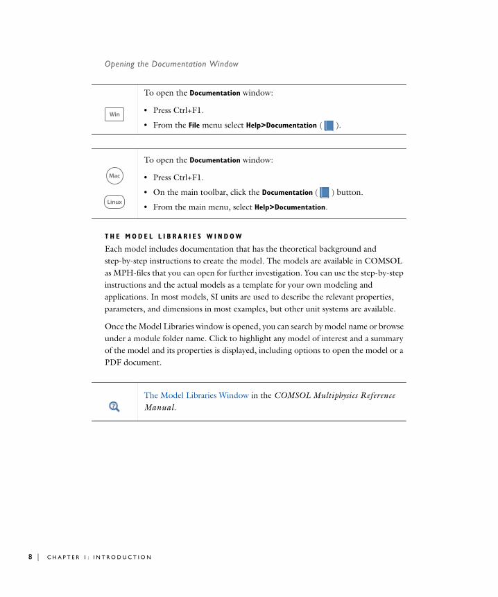
Opening the Documentation Window

T H E M O D E L L I B R A R I E S W I N D O W

Each model includes documentation that has the theoretical background and step-by-step instructions to create the model. The models are available in COMSOL as MPH-files that you can open for further investigation. You can use the step-by-step instructions and the actual models as a template for your own modeling and applications. In most models, SI units are used to describe the relevant properties, parameters, and dimensions in most examples, but other unit systems are available.

Once the Model Libraries window is opened, you can search by model name or browse under a module folder name. Click to highlight any model of interest and a summary of the model and its properties is displayed, including options to open the model or a PDF document.

To open the Documentation window:

• Press Ctrl+F1.

• From the File menu select Help>Documentation ( ).

To open the Documentation window:

• Press Ctrl+F1.

• On the main toolbar, click the Documentation ( ) button.

• From the main menu, select Help>Documentation.

The Model Libraries Window in the COMSOL Multiphysics Reference Manual.


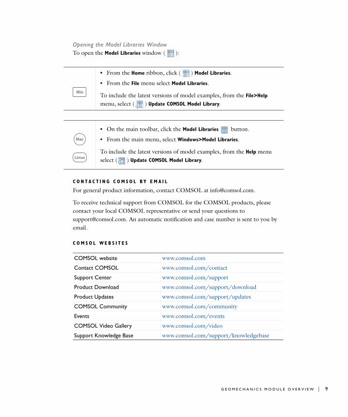
Opening the Model Libraries WindowTo open the Model Libraries window ( ):

C O N T A C T I N G C O M S O L B Y E M A I L

For general product information, contact COMSOL at [email protected].

To receive technical support from COMSOL for the COMSOL products, please contact your local COMSOL representative or send your questions to [email protected]. An automatic notification and case number is sent to you by email.

C O M S O L WE B S I T E S

• From the Home ribbon, click ( ) Model Libraries.

• From the File menu select Model Libraries.

To include the latest versions of model examples, from the File>Help menu, select ( ) Update COMSOL Model Library.

• On the main toolbar, click the Model Libraries button.

• From the main menu, select Windows>Model Libraries.

To include the latest versions of model examples, from the Help menu select ( ) Update COMSOL Model Library.

COMSOL website www.comsol.com

Contact COMSOL www.comsol.com/contact

Support Center www.comsol.com/support

Product Download www.comsol.com/support/download

Product Updates www.comsol.com/support/updates

COMSOL Community www.comsol.com/community

Events www.comsol.com/events

COMSOL Video Gallery www.comsol.com/video

Support Knowledge Base www.comsol.com/support/knowledgebase

G E O M E C H A N I C S M O D U L E O V E R V I E W | 9

http://www.comsol.com

http://www.comsol.com/contact/

http://www.comsol.com/support/

http://www.comsol.com/support/download/

http://www.comsol.com/support/updates

http://www.comsol.com/community

http://www.comsol.com/events/

http://www.comsol.com/video/

http://www.comsol.com/support/knowledgebase/

10 | C H A P T E R

2

G e o m e c h a n i c s T h e o r y

The Geomechanics Module contains new materials which are used in combination with the Structural Mechanics Module to account for the plasticity of soils and failure criteria in rocks, concrete and other brittle materials.

In this chapter:

• General Geomechanics Theory

• Defining Perfectly Plastic Materials

• Plasticity Models for Soils

• Theory for the Cam-Clay Material

• Failure Criteria for Concrete, Rocks, and Other Brittle Materials

• Elastoplastic Material Theory

• Creep and Viscoplasticity

• References for the Geomechanics Module

11

12 | C H A P T E R

Gene r a l G eome chan i c s T h e o r y

In this section:

• Sign Conventions for Stress and Strain Analysis

• Defining the Stress Invariants

• Defining the Yield Surface

Sign Conventions for Stress and Strain Analysis

The theory of plasticity was initially developed in continuum mechanics where tensile stresses are usually considered to be positive quantities and compressive stresses are negative quantities. Under this convention, force and displacement components are considered positive if directed in the positive directions of the coordinate axes. Tensile normal strains and tensile normal stresses are treated as positive (Ref. 11).

Engineering analysis and design for soil and rock structures, however, are in most cases concerned with compressive stresses (Ref. 1). Therefore, in geotechnical applications the opposite sign convention is usually adopted because compressive normal stresses are more common than tensile ones (Ref. 5).

The Geomechanics Module follows the sign convention of continuum mechanics as stated in Ref. 1 (positive tensile stresses). This is consistent with the notation used in the Structural Mechanics Module. This means the principal stresses often have a negative sign, and are sorted as 123.

The convention used in Ref. 1 refers to the hydrostatic pressure (trace of the stress Cauchy tensor) with a positive sign. The use of the first invariant of Cauchy stress tensor I1() is preferred through this document, in order to avoid misunderstandings with the convention in the Structural Mechanics Module (where pressure is positive under compression, or equivalently, it has the opposite sign of the Cauchy stress tensor’s trace).

Theory for the Solid Mechanics Interface in the Structural Mechanics Module User’s Guide

2 : G E O M E C H A N I C S T H E O R Y

Defining the Stress Invariants

The starting point for defining the theory of plastic deformation of soils is the definition of the first, second, and third invariants for the Cauchy stress tensor . These invariants are defined as follows:

(2-1)

The first invariant I1 is the trace of the tensor, the second invariant I2 is the sum of the principal two-rowed minors of the determinant of , and the third invariant I3 is the determinant of . (Ref. 1).

When 1, 2, and 3, represent the principal components of the stress tensor, these invariants can be written as

The principal components of the stress tensor are the roots of the characteristic equation (Cayley–Hamilton theorem)

which comes from calculating the roots for the equation

Defining the deviatoric stress as the traceless tensor

I1 trace =

I2 12--- I1

2 :– =

I3 det =

I1 1 2 3+ +=

I2 12 23 13+ +=

I3 1 2 3 =

3 I12

– I2 I3–+ 0=

det I– 0=

The invariants I1, I2, and I3 can be called in user-defined yield criteria by referencing the corresponding variables solid.I1s, solid.I2s, and solid.I3s.

dev 13---I1I–=

G E N E R A L G E O M E C H A N I C S T H E O R Y | 13

14 | C H A P T E R

introduces us to the first, second, and third deviatoric stress invariants

(2-2)

As defined above J20. In soil plasticity, the most relevant invariants are I1, J2, and J3. I1 represents the effect of mean stress, J2 represents the magnitude of shear stress, and J3 is the direction of the shear stress.

O T H E R I N V A R I A N T S

It is possible to define other invariants in terms of the primary invariants. One common auxiliary invariant is the Lode angle

(2-3)

The Lode angle is bounded to 03 when the principal stresses are sorted as 123 (Ref. 1).

Following this convention, =corresponds to the tensile meridian, and =3corresponds to the compressive meridian. The Lode angle is part of a cylindrical coordinate system (the Haigh–Westergaard coordinates) with height (hydrostatic axis)

and radius .

J1 trace dev = 0=

J2 12---dev :dev =

J3 det dev =

The invariants J2 and J3 can be called in user-defined yield criteria by referencing the variables solid.II2s and solid.II3s, where solid is the name of the interface identifier for the physics interface.

3cos 3 32

-----------J3

J23 2

------------=

I1/ 3= r 2J2=

The Lode angle is undefined at the hydrostatic axis, where all three principal stresses are equal (1=2=3=I1/3) and J2=0. To avoid division by zero, the Lode angle is computed from the inverse tangent function atan2, instead of the inverse cosine, as stated in Equation 2-3.


The octahedral plane (also called -plane) is defined perpendicular to the hydrostatic axis in the Haigh–Westergaard coordinate system. The stress normal to this plane is oct=I1/3, and the shear stress on that plane is defined by

The functions described in Equation 2-1 and Equation 2-2 enter into expressions that define various kind of yield and failure surfaces. A yield surface is a surface in the 3D space of principal stresses which circumscribe an elastic state of stress.

P R I N C I P A L S T R E S S E S

The principal stresses 1, 2, and 3) are the eigenvalues of the stress tensor, and when sorted as 123 they can be written by using the invariants I1 and J2 and the Lode angle 03 (Ref. 1):

here, i0 means tensile stress, and i0 means compressive stress.

Defining the Yield Surface

A yield criterion serves to define the stress condition under which plastic deformation occurs. Stress paths within the yield surface result in purely recoverable deformations

The Lode angle and the effective (von Mises) stress can be called in user-defined yield criteria by referencing the variables solid.thetaL and solid.mises, where solid is the name of the interface identifier for the physics interface.

oct 2/3J2=

1 =13---I1

4J23

---------- cos+

2 =13---I1

4J23

---------- 23

------– cos+

3 =13---I1

4J23

---------- 23

------+ cos+

The principal stresses can be called in user-defined yield criteria by referencing the variables solid.sp1, solid.sp2 and solid.sp3.

G E N E R A L G E O M E C H A N I C S T H E O R Y | 15

16 | C H A P T E R

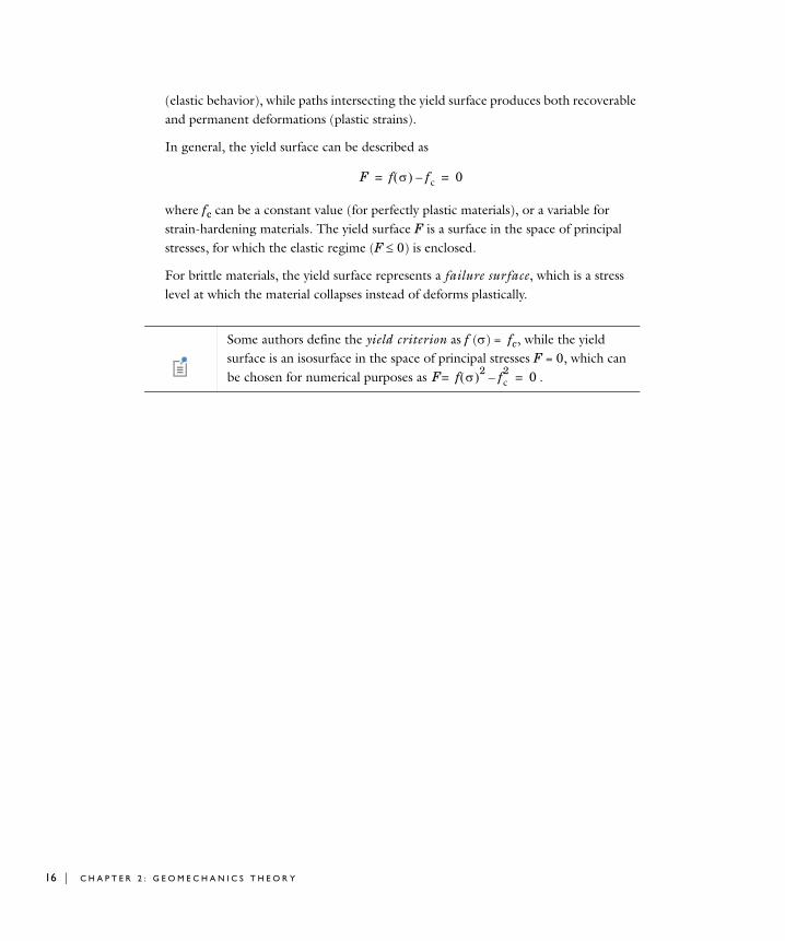
(elastic behavior), while paths intersecting the yield surface produces both recoverable and permanent deformations (plastic strains).

In general, the yield surface can be described as

where fc can be a constant value (for perfectly plastic materials), or a variable for strain-hardening materials. The yield surface F is a surface in the space of principal stresses, for which the elastic regime (F0) is enclosed.

For brittle materials, the yield surface represents a failure surface, which is a stress level at which the material collapses instead of deforms plastically.

F f fc– 0= =

Some authors define the yield criterion as f ()= fc, while the yield surface is an isosurface in the space of principal stresses F=0, which can be chosen for numerical purposes as . F f 2= fc

2– 0=


De f i n i n g P e r f e c t l y P l a s t i c Ma t e r i a l s

For perfect elastoplastic materials, the yield surface is fixed in the 3D space of principal stress, and therefore, plastic deformations occur only when the stress path moves on the yield surface (the regime inside the yield surface is elastic, and stress paths beyond the yield surface are not allowed).

In general, the yield criterion depends on various parameters. Most of the plasticity models are based on isotropic assumptions, which require the yield function to be independent of the chosen coordinate system. This introduces the concept of using the stress invariants previously defined in Equation 2-1, Equation 2-2, and Equation 2-3.

In this section:

• von Mises Criterion

• Tresca Criterion

von Mises Criterion

The von Mises criterion suggests that the yielding of the material begins when the second deviatoric stress invariant J2 reaches a critical value. This criterion can be written in terms of the elements of Cauchy’s stress tensor (Ref. 1)

or equivalently .

The von Mises criterion is implemented as

where ys is the yield stress level (yield stress in uniaxial tension).

J216--- 11 22– 2 22 33– 2 33 11– 2+ + 12

2 232 13

2+ + + k2= =

J2 k=

F 3J2 ys– 0= =

The effective or von Mises stress ( ) is available in the variable solid.mises, where solid is the name of the interface identifier for the physics interface.

mises 3J2=

D E F I N I N G P E R F E C T L Y P L A S T I C M A T E R I A L S | 17

18 | C H A P T E R

Tresca Criterion

The Tresca yield surface is normally expressed in terms of the principal stress components

The Tresca criterion is a hexagonal prism with its axis equally inclined to the three principal stress axes. When the principal stresses fulfill 123, this criterion is written as

By using the representation of principal stresses in term of the invariants J2 and the Lode angle 03, this criterion can alternatively be written as

or equivalently

The maximum shear stress is reached at the meridians (=0 or =). The Tresca criterion can be circumscribed by setting the Lode angle =0, or equivalently, by a von Mises criterion

The minimum shear is reached at=, so the Tresca criterion can be inscribed by setting a von Mises criterion

When dealing with soils, the parameter k is also called undrained shear strength.

12---max 1 2– 1 3– 2 3– k=

12--- 1 3– k=

12---

4J23

---------- 23

------+ cos–cos

J2 3---+

sin k= =

J2 6---–

cos k=

3J2 2k=

J2 k=

The Tresca effective stress, tresca=13 is implemented in the variable solid.tresca, where solid is the name of the interface identifier for the physics interface.


Figure 2-1: The upper and lower limits of the Tresca criterion.

Figure 2-2: Classical yield criteria for metals. Left: Tresca criterion. Right: von Mises criterion.

The von Mises and Tresca criteria are independent of the first stress invariant I1 and are mainly used for the analysis of plastic deformation in metals and ductile materials, though some researchers also use these criteria for describing fully saturated cohesive soils (that is, clays) under undrained conditions.

Upper limit

Lower limit

D E F I N I N G P E R F E C T L Y P L A S T I C M A T E R I A L S | 19

20 | C H A P T E R

P l a s t i c i t y Mode l s f o r S o i l s

In this section:

• Mohr-Coulomb Criterion

• Drucker-Prager Criterion

• Matsuoka-Nakai Criterion

• Lade-Duncan Criterion

• Tension Cut-Off

Mohr-Coulomb Criterion

The Mohr-Coulomb criterion is the most popular criterion in soil mechanics. It was developed by Coulomb before the Tresca and von Mises criteria for metals, and it was the first criterion to account for the hydrostatic pressure. The criterion states that failure occurs when the shear stress and the normal stress acting on any element in the material satisfy the equation

here, is the shear stress, c the cohesion, and denotes the angle of internal friction.

With the help of Mohr’s circle, this criterion can be written as

The Mohr-Coulomb criterion defines an irregular hexagonal pyramid in the space of principal stresses, which generates singularities in the derivatives of the yield function.

Elastoplastic Material Theory

tan c–+ 0=

12--- 1 3– 1

2--- 1 3+ c– cossin+ 0=


Figure 2-3: The Mohr-Coulomb criterion.

The Mohr-Coulomb criterion can be written in terms of the invariants I1 and J2 and the Lode angle 03 (Ref. 1, Ref. 9) when the principal stresses are sorted as 123. The yield function then reads

The tensile meridian is defined when =and the compressive meridian when =.

Rearranging terms, the Mohr-Coulomb criterion reads

where

, , and

In the special case of frictionless material, ( , =0, k=c), the Mohr-Coulomb criterion reduces to a Tresca’s maximum shear stress criterion, 13=2k or equivalently

Tens

ile m

erid

ian

Compressiv

e meri

dian

Fy13---I1

J23------ 1 sin+ 1 sin– 2

3------+

cos–cos c cos–+sin 0= =

Fy J2m I1 k–+ 0= =

m 6– cos 1 3 sin 6– sin–= 3sin= k c cos=

0=

Fy J2 6---–

cos k– 0= =

P L A S T I C I T Y M O D E L S F O R S O I L S | 21

22 | C H A P T E R

Drucker-Prager Criterion

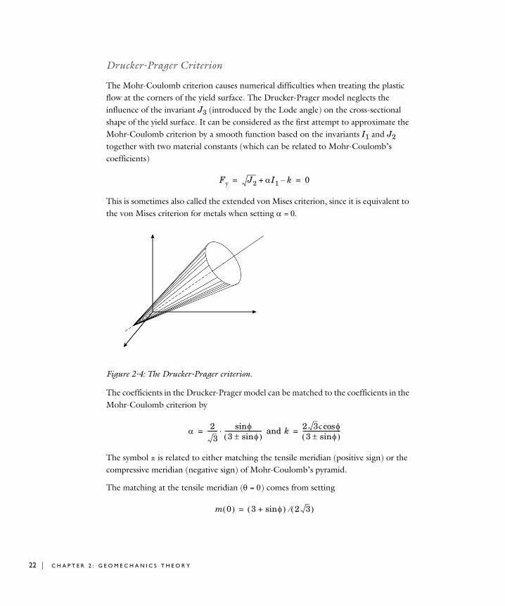
The Mohr-Coulomb criterion causes numerical difficulties when treating the plastic flow at the corners of the yield surface. The Drucker-Prager model neglects the influence of the invariant J3 (introduced by the Lode angle) on the cross-sectional shape of the yield surface. It can be considered as the first attempt to approximate the Mohr-Coulomb criterion by a smooth function based on the invariants I1 and J2 together with two material constants (which can be related to Mohr-Coulomb’s coefficients)

This is sometimes also called the extended von Mises criterion, since it is equivalent to the von Mises criterion for metals when setting =

Figure 2-4: The Drucker-Prager criterion.

The coefficients in the Drucker-Prager model can be matched to the coefficients in the Mohr-Coulomb criterion by

and

The symbol ± is related to either matching the tensile meridian (positive sign) or the compressive meridian (negative sign) of Mohr-Coulomb’s pyramid.

The matching at the tensile meridian (=) comes from setting

Fy J2 I1 k–+ 0= =

23

------- sin3 sin

--------------------------= k 2 3c cos3 sin

---------------------------=

m 0 3 sin+ 2 3 =


in the Mohr-Coulomb criterion, and the matching at the compressive meridian (=) from setting

Figure 2-5: The Drucker-Prager criterion showing the tensile and compressive meridians (inner and outer circles), and the Lode angle compared to the cross section of Mohr-Coulomb criterion in the -plane.

In the special case of frictionless material, (=0, =0, ), the Drucker -Prager criterion reduces to the von Mises criterion

When matching Drucker-Prager criterion to Mohr-Coulomb criterion in 2D plane-strain applications, the parameters are

and

and when matching both criteria in 2D plane-stress applications, the matching parameters are:

and

m 3 3 sin– 2 3 =

Tensile meridianCompressive meridian

k 2c 3=

J2 2c 3=

= tan

9 12 2tan+------------------------------------ k = 3c

9 12 2tan+------------------------------------

= 13

------- sin k = 23

------- c cos


24 | C H A P T E R

D I L A T A T I O N A N G L E

The Mohr-Coulomb yield criterion is sometimes used with a nonassociated plastic potential. This plastic potential could be either a Drucker-Prager criterion, or the same Mohr-Coulomb yield function but with a different slope with respect to the hydrostatic axis, in which case the angle of internal friction is replaced by the dilatation angle, which is normally smaller (Ref. 5).

Also, when using a Drucker-Prager criterion matched to a Mohr-Coulomb criterion, the plastic potential could also be nonassociated, in which case the difference between the dilatation angle and the angle of internal friction would result in a yield surface and plastic potential portrayed by two cones with different angles with respect to the hydrostatic angle.

E L L I P T I C C A P

The Mohr-Coulomb and Drucker-Prager criteria portray a conic yield surface which is open in the hydrostatic axis direction. Normally, these soil models are not accurate above a given limit pressure because real-life materials cannot bear infinite loads and still behave elastically. A simple way to overcome this problem is to add an elliptical end-cap to these soil models.

The elliptic cap is an elliptic yield surface of a semi-axes as shown in Figure 2-6. The initial pressure pa (SI units: Pa) denotes the pressure at which the elastic range circumscribed by either a Mohr-Coulomb pyramid or a Drucker-Prager cone is not valid any longer, so a cap surface is added. The limit pressure pb gives the curvature of the ellipse, and denotes the maximum admissible hydrostatic pressure for which the material starts deforming plastically. Pressures higher than pb are not allowed

Figure 2-6: Elliptic cap model in Haigh–Westergaard coordinate system.

ppbpa

q


Note that the sign convention for the pressure is taken from the Structural Mechanics Module: positive sign under compression, so pa and pb are positive parameters. Figure 2-6 shows the cap in terms of the variables

and

Matsuoka-Nakai Criterion

Matsuoka and Nakai (Ref. 3) discovered that the sliding of soil particles occurs in the plane in which the ratio of shear stress to normal stress has its maximum value, which they called the mobilized plane. They defined the yield surface as

where the parameter =/nSTP equals the maximum ratio between shear stress and normal stress in the spatially mobilized plane (STP-plane), and the invariants are applied over the effective stress tensor (this is the Cauchy stress tensor minus the fluid pore pressure).

The Matsuoka-Nakai criterion circumscribes the Mohr-Coulomb criterion in dry soils, when

and denotes the angle of internal friction in Mohr-Coulomb criterion.

Figure 2-7: The Matsuoka-Nakai criterion and Mohr-Coulomb criterion in the principal stress space.

q 3J2 = p I– 1 3=

Fy 9 92+ I3 I1I2– 0= =

2 23

----------- tan=


26 | C H A P T E R

Lade-Duncan Criterion

The Lade-Duncan criterion was originally developed to model a large volume of laboratory sample test data of cohesionless soils. This criterion is defined as

where I1 and I3 are the first and third stress invariants respectively, and k is a parameter related to the direction of the plastic strain increment in the triaxial plane. The parameter k can vary from 27 for hydrostatic stress conditions (1=2=3), up to a critical value kc at failure. In terms of the invariants I1, J2,and J3, this criterion can be written as

The Lade-Duncan criterion can be fitted to the compressive meridian of the Mohr-Coulomb surface by choosing

with as the angle of internal friction in Mohr-Coulomb criterion

Figure 2-8: Comparing the Mohr-Coulomb, Matsuoka-Nakai, and Lade-Duncan criteria when matching the tensile meridian.

Fy kI3 I13

– 0= =

Fy J313---I1J2–

127------ 1

k---–

I13

+ 0= =

k 3 sin– 3/ 2 1 sin– cos =

Mohr-Coulomb

Matsuoka-NakaiLade-Duncan

The Lade-Duncan criterion does not match the Mohr-Coulomb criterion (nor the Matsuoka-Nakai criterion) at the tensile meridian.


Tension Cut-Off

It appears that the Mohr-Coulomb and Drucker-Prager criteria predict tensile strengths larger than the experimental measurements on soil samples. This discordance can be mended by the introduction of the Rankine or tension cut-off criterion.

The Rankine criterion states that a material stops deforming elastically when the biggest principal stress 1 reaches a maximum tensile stress, also called tension cut-off limit t.

In terms of the principal stress, Rankine criterion reads

For soils and clays, the maximum tensile stress can be estimated from the material parameters, such as the cohesion c and the friction angle For instance, the tip of the cone in Mohr-Coulomb criterion is reached when

therefore, the tension cut-off should be chosen such as

The Mohr-Coulomb criterion together with a tension cut-off is sometimes called modified Mohr-Coulomb criterion (Ref. 19).

F 1 t– 0= =

1 c cossin

------------=

t c cossin

------------

Tension cut-off is also available with Concrete material models.


28 | C H A P T E R

Th eo r y f o r t h e C am-C l a y Ma t e r i a l

In this section:

• About the Cam-clay Material

• Volumetric Elastic Behavior

• Hardening and Softening

• Including Pore Fluid Pressure

About the Cam-clay Material

The Cam-clay material model was developed at the University of Cambridge in the 1970s, and since then it has experienced different modifications. The modified Cam-clay model is the most commonly used due to the smooth yield surface, and it is the one implemented in the Geomechanics Module.

The Cam-clay model is a so-called critical state model, where the loading and unloading of the material follows different trajectories in stress space. The model also features hardening and softening of clays. Different formulations can be found in textbooks about these models (see Ref. 13, 14, and 15).

The yield function is written in terms of the variables

and

Following the Structural Mechanics Module sign convention:

This is an ellipse in p-q plane, with a cross section independent of Lode angle and smooth for differentiation. Note that p, q and pc are always positive variables.

The material parameter M0 defines the slope of a line in the p-q space called critical state line, and it can be related to the angle of internal friction in the Mohr-Coulomb criterion

q 3J2 = p I– 1 3=

Fy q2 M2 p pc– p+ 0= =

M 6 sin3 sin–--------------------------=


Figure 2-9: Modified Cam-clay surface in the p-q plane. The ellipse circumscribes a nonlinear elastic region.

In the Cam-clay model, hardening is controlled by the consolidation pressure pc, which depends exponentially on the volumetric plastic strain pvol.

(2-4)

Here, the parameter pc0 is the initial consolidation pressure, and the exponent Bp is a parameter which depends on the initial void ratio e0, the swelling index , and the compression index

The initial void ratio, the compression index, and the swelling index are all positive parameters and must fulfill

, so

Nonlinear elastic region

hardening

Critical state linesoftening

qq = Mp

pc ppc/2

pc pc0eBppvol–

=

The volumetric plastic strain is available in the variable solid.epvol and the consolidation pressure in the variable solid.Pc.

Bp1 e0+

–---------------=

0 Bp 0

T H E O R Y F O R T H E C A M - C L A Y M A T E R I A L | 29

30 | C H A P T E R

In this formulation, the compression index is the slope of the virgin isotropic consolidation line, and is the slope of the rebound-reloading line (also called loading-reloading line) in the e versus ln(p) plane.

Figure 2-10: Slopes of the virgin isotropic consolidation line, and rebound-reloading line in the e vs. ln(p) plane. The reference void ratio N is measured at the reference pressure prefN.

Volumetric Elastic Behavior

The stress-strain relation beyond the elastic range is of great importance in soil mechanics. For additive decomposition of strains, Cauchy’s stress tensor is written as

Here, is the Cauchy stress tensor, is the total strain tensor, 0 and 0 are the initial stress and strain tensors, th is the thermal strain tensor, p is the plastic strain tensor, c is the creep strain tensor, and, C is the fourth-order elasticity tensor.

The void ratio e is the ratio between pore volume and solid volume. It can be written in terms of the porosity as e= /(1 ).

ln(p)

N

ln(prefN) ln(pC0)

e

If an Initial Stress and Strain feature subnode is added to the Cam-clay material, the initial consolidation pressure pc0 must be made equal or bigger than one third of minus the trace of the initial stress tensor, otherwise the initial stress state is outside the Cam-clay ellipse.

0– C: 0– th– p– c– =


For a linear elastic material, the trace of the Cauchy’s stress tensor is linearly related to the volumetric elastic strain (the trace of the elastic strain tensor) by the elastic bulk modulus

here p0=trace0/3 is the trace of the initial stress tensor 0, and K is the bulk modulus, a constant parameter independent of the stress or strain.

The modified Cam-clay model introduces a nonlinear relation between stress and volumetric elastic strain

with

and K0 a reference bulk modulus. This formulation gives a tangent bulk modulus KTBepp0. The reference bulk modulus is calculated from the initial consolidation pressure pc0, and the void ratio at reference pressure N.

Hardening and Softening

The yield surface for the modified Cam-clay model reads

The associated flow rule (Qp=Fy) and the yield surface written in terms of these two invariants, Fy(I1, J2), gives a rate equation for the plastic strain tensor calculated from the derivatives of Fy with respect to the stress tensor

p I– 1 3 p0 Kelvol–= =

The elastic volumetric strain is available in the variable solid.eelvol.

p p0– K– 0eBeelvol–

= Be1 e0+

---------------=

Fy q2 M2 p pc– p+ 0= =

·p pQp

---------- pQpI1----------

I1--------

QpJ2----------

J2---------+

= =

Here, p means the plastic multiplier, see Plastic Flow for Small Strains and Hardening Models.

T H E O R Y F O R T H E C A M - C L A Y M A T E R I A L | 31

32 | C H A P T E R

The plastic strain rate tensor includes both deviatoric and isotropic parts. Note that

and

These relations can be used for writing the plastic flow as

The trace of the plastic strain rate tensor (the volumetric plastic strain rate ) then reads

This relation explains the reason why there is isotropic hardening for p>pc/2 and isotropic softening for p<pc/2. So the volumetric plastic strain can either increase or decrease.

In the Cam-clay model, the hardening is controlled by the consolidation pressure variable as a function of volumetric plastic strain, as written in Equation 2-4. Hardening introduces changes in the shape of the Cam-clay ellipse, since its major semiaxis depends on the value of pc.

Including Pore Fluid Pressure

When a pore fluid pressure pf is added to the Cam-clay material, the yield surface is shifted on the p axis

The quantity ppf is normally regarded as the effective pressure, or effective stress, which should not be confused with von Mises stress.

·p

I1 I= J2 dev =

·p p13---Qpp

----------– IQpq

---------- 32q-------dev +

p13---M2 2p pc– – I 3dev +

= =

·pvol

·pvol trace ·p p M2 2p pc– – = =

pc pvol

Fy q2 M2 p pf– pc– p pf– + 0= =


F a i l u r e C r i t e r i a f o r C on c r e t e , Ro c k s , a nd O t h e r B r i t t l e Ma t e r i a l s

In this section:

• Bresler-Pister Criterion

• Willam-Warnke Criterion

• Ottosen Criterion

• Original Hoek-Brown Criterion

• Generalized Hoek-Brown Criterion

Bresler-Pister Criterion

The Bresler-Pister criterion (Ref. 2) was originally devised to predict the strength of concrete under multiaxial stresses. This failure criterion is an extension of the Drucker-Prager criterion to brittle materials and can be expressed in terms of the stress invariants as

(2-5)

here, k1, k2, and k3 are material parameters.

This criterion can also be written (Ref. 17) in term of the uniaxial compressive strength fc and the octahedral normal and shear stresses

and

so Equation 2-5 simplifies to

Here, the parameters a, b, and c are obtained from the uniaxial compression, uniaxial tension, and biaxial compression tests, respectively. The octahedral normal stress octis considered positive when tensile, and fc is taken positive.

Fy J2 k1I12 k2I1 k3+ + + 0= =

oct = I1/3 oct 2J2/3=

Fyoctfc

--------- a– boctfc

---------- coct

2

fc2

----------–+ 0= =

F A I L U R E C R I T E R I A F O R C O N C R E T E , R O C K S , A N D O T H E R B R I T T L E M A T E R I A L S | 33

34 | C H A P T E R

Willam-Warnke Criterion

The Willam-Warnke criterion (Ref. 10) is used to predict failure in concrete and other cohesive-frictional materials such as rock, soil, and ceramics. Just as the Bresler-Pister criterion, it depends only on three parameters. It was developed to describe initial concrete failure under triaxial conditions. The failure surface is convex, continuously differentiable, and is fitted to test data in the low compression range. The material is considered perfect elastoplastic (no hardening).

The original “three-parameter” Willam-Warnke failure criterion was defined as

(2-6)

here, fc is the uniaxial compressive strength, ft is uniaxial tensile strength, and fb is obtained from the biaxial compression test. All parameters are positive. The octahedral normal and shear stresses are defined as usual

, and

This can be written as

with

The function r( describes the segment of an ellipse on the octahedral plane when . By using the Lode angle , the dimensionless function r( is defined as

Here, the tensile and compressive meridian rt and rc are defined in terms of the positive parameters fc, fb, and ft:

Fy35---octfc

--------- r 1ft--- 1

fb----–

oct 1– 0=+=

oct = I1/3 oct 2J2/3=

Fy J252---r 1

3------I1 fc– 0=+=

fbft/ fbfc ftfc– =

0 3

r 2rc rc

2 rt2– rc 2rt rc– 4 rc

2 rt2– 5rt

2 4– rcrt+2

cos+cos

4 rc2 rt

2– rc 2rt– 2+2

cos---------------------------------------------------------------------------------------------------------------------------------------------------------------=

rt =65---

fbft2fbfc ftfc+----------------------------


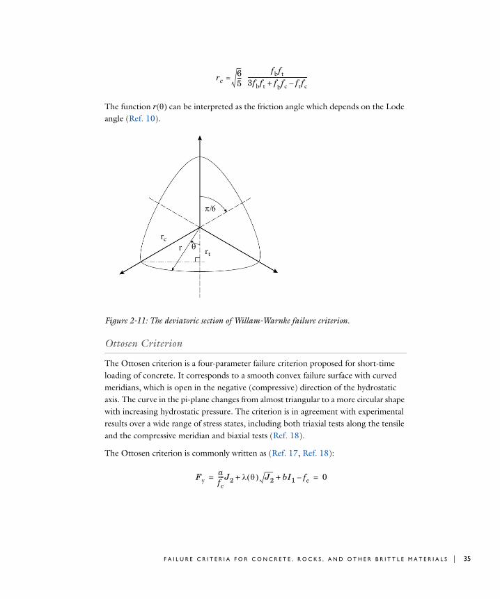
The function r( can be interpreted as the friction angle which depends on the Lode angle (Ref. 10).

Figure 2-11: The deviatoric section of Willam-Warnke failure criterion.

Ottosen Criterion

The Ottosen criterion is a four-parameter failure criterion proposed for short-time loading of concrete. It corresponds to a smooth convex failure surface with curved meridians, which is open in the negative (compressive) direction of the hydrostatic axis. The curve in the pi-plane changes from almost triangular to a more circular shape with increasing hydrostatic pressure. The criterion is in agreement with experimental results over a wide range of stress states, including both triaxial tests along the tensile and the compressive meridian and biaxial tests (Ref. 18).

The Ottosen criterion is commonly written as (Ref. 17, Ref. 18):

rc =65---

fbft3fbft f+ bfc ftfc–-------------------------------------------

rc

rtr

Fyafc----J2 J2 bI1 fc–+ + 0= =


36 | C H A P T E R

In this formulation, the parameters a>0, b>0, k1>0, and k2>0 are dimensionless, and fc>0 is the uniaxial compressive strength of concrete (with a positive sign). The function (dimensionless) is defined as

The parameter k1 is called the size factor. The parameter k2 (also called shape factor) is positive and bounded to 0k21(Ref. 17, Ref. 18).

Typical values for these parameters are obtained by curve-fitting the uniaxial compressive strength fc, uniaxial tensile strength ft, and from the biaxial and triaxial data (for instance, a typical biaxial compressive strength of concrete is 16% higher than the uniaxial compressive strength). The parameters fc, fb, and ft are positive.

The compressive and tensile meridians (as defined in the Willam-Warnke criterion) are

For concrete, the ratio

TABLE 2-1: TYPICAL PARAMETER VALUES FOR OTTOSEN FAILURE CRITERION (Ref. 18).

ft/ fc a b k1 k2 lt lc0.08 1.8076 4.0962 14.4863 0.9914 14.4725 7.7834

0.10 1.2759 3.1962 11.7365 0.9801 11.7109 6.5315

0.12 0.9218 2.5969 9.9110 0.9647 9.8720 5.6979

0

k113--- k2 3 cos acos J3 0cos

k13--- 1

3---– k– 2 3 cos acos

J3 0,cos

=

rc = 1c----- = 1

/3 -------------------

rt = 1t----- = 1

0 -----------

c/t rt/rc=


normally lies between 0.54~0.58.

Original Hoek-Brown Criterion

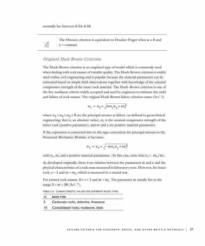
The Hoek-Brown criterion is an empirical type of model which is commonly used when dealing with rock masses of variable quality. The Hoek-Brown criterion is widely used within civil engineering and is popular because the material parameters can be estimated based on simple field observations together with knowledge of the uniaxial compressive strength of the intact rock material. The Hoek–Brown criterion is one of the few nonlinear criteria widely accepted and used by engineers to estimate the yield and failure of rock masses. The original Hoek-Brown failure criterion states (Ref. 5)

where 1230 are the principal stresses at failure (as defined in geotechnical engineering; that is, an absolute value), c is the uniaxial compressive strength of the intact rock (positive parameter), and m and s are positive material parameters.

If the expression is converted into to the sign convention for principal stresses in the Structural Mechanics Module, it becomes

with c, m, and s positive material parameters. (In this case, note that 1 sc/m).

As developed originally, there is no relation between the parameters m and s and the physical characteristics of a rock mass measured in laboratory tests. However, for intact rock, s1 and mmi, which is measured in a triaxial test.

For jointed rock masses, 0s1 and mmi. The parameter m usually lies in the range 5m30 (Ref. 7).

The Ottosen criterion is equivalent to Drucker-Prager when a = 0 and = constant.

TABLE 2-2: CHARACTERISTIC VALUES FOR DIFFERENT ROCK TYPES

m ROCK TYPE

5 Carbonate rocks, dolomite, limestone

10 Consolidated rocks, mudstone, shale

1 3 mc3 sc2++=

1 3 mc1– sc2++=


38 | C H A P T E R

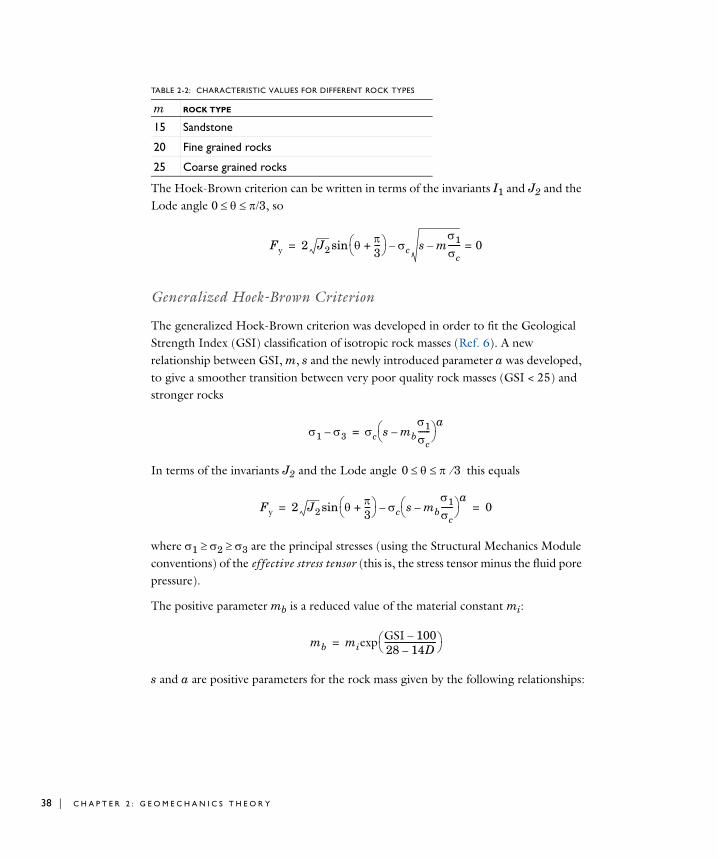
The Hoek-Brown criterion can be written in terms of the invariants I1 and J2 and the Lode angle 03, so

Generalized Hoek-Brown Criterion

The generalized Hoek-Brown criterion was developed in order to fit the Geological Strength Index (GSI) classification of isotropic rock masses (Ref. 6). A new relationship between GSI, m, s and the newly introduced parameter a was developed, to give a smoother transition between very poor quality rock masses (GSI<25) and stronger rocks

In terms of the invariants J2 and the Lode angle this equals

where 123 are the principal stresses (using the Structural Mechanics Module conventions) of the effective stress tensor (this is, the stress tensor minus the fluid pore pressure).

The positive parameter mb is a reduced value of the material constant mi:

s and a are positive parameters for the rock mass given by the following relationships:

15 Sandstone

20 Fine grained rocks

25 Coarse grained rocks

TABLE 2-2: CHARACTERISTIC VALUES FOR DIFFERENT ROCK TYPES

m ROCK TYPE

Fy 2 J2 3---+

c s m1c------– 0=–sin=

1 3– c s mb1c------–

a=

0 3

Fy 2 J2 3---+

c s mb1c------–

a–sin 0= =

mb miexp GSI 100–28 14D–-------------------------- =


The disturbance factor D was introduced to account for the effects of stress relaxation and blast damage, and it varies from 0 for undisturbed in-situ rock masses to 1 for very damaged rock masses.

TABLE 2-3: DISTURBANCE FACTOR IN ROCK MASSES

D DESCRIPTION OF ROCK MASS

0 Undisturbed rock mass

0~0.5 Poor quality rock mass

0.8 Damaged rock mass

1.0 Severely damaged rock mass

s = exp GSI 100–9 3D–

--------------------------

a = 12--- 1

6--- exp GSI–

15------------- exp 20–

3--------- –

+


40 | C H A P T E R

E l a s t o p l a s t i c Ma t e r i a l T h e o r y

In this section:

• Introduction to Small and Large Plastic Strains

• Plastic Flow for Small Strains

• Isotropic Plasticity

• Yield Function

• Hardening Models

• Plastic Flow for Large Strains

• Numerical Solution of the Elastoplastic Conditions

• References for Elastoplastic Materials

Introduction to Small and Large Plastic Strains

There are two implementations of plasticity available in COMSOL Multiphysics. One is based on the additive decomposition of strains, which is the most suitable approach in the case of small strains, and the other one is based on the multiplicative decomposition of the deformation gradient, which is more suitable when large plastic strains occurs.

The additive decomposition of strains is used when small plastic strain is selected as the plasticity model. The stress-strain relationship is then written as

Here:

• is the Cauchy stress tensor

• is the total strain tensor

• 0 and 0 are the initial stress and strain tensors

• th is the thermal strain tensor

Working with the Geomechanics Materials

0– C: 0– th– p– c– =


• p is the plastic strain tensor

• c is the creep strain tensor, and

• C is the fourth-order elasticity tensor.

The elastic strain tensor is computed by removing inelastic and initial strains from the total strain tensor

In the special case of zero initial strains and no creep or thermal expansion, the elastic strain tensor simplifies to

(2-7)

If or p are large, the additive decomposition might produce incorrect results; however, the additive decomposition of strains is widely use for metal and soil plasticity.

When large plastic strain is selected as the plasticity model, the total deformation gradient tensor is multiplicatively decomposed into elastic deformation gradient and plastic deformation gradient

The plastic deformation is removed from the total deformation gradient,

so the elastic Green-Lagrange strain tensor is computed from the elastic deformation gradient tensor Fel

el 0– th– p– c–=

el p–=

When Small plastic strain is selected as the plasticity model for the Plasticity node, and the Include geometric nonlinearity check box is selected on the study settings window, the second Piola-Kirchhoff stress is used instead of the Cauchy stress, and the additive decomposition of strains is understood as the summation of Green-Lagrange strains.

F FelFp=

Fel FFp 1–

=

el12--- Fel

T Fel I– =

E L A S T O P L A S T I C M A T E R I A L T H E O R Y | 41

42 | C H A P T E R

and the plastic Green-Lagrange strain tensor is computed from the plastic deformation gradient tensor

As opposed to the small strain formulation described in Equation 2-7, the total, plastic and elastic Green-Lagrange strain tensors are related as

Under multiplicative decomposition, the elastic right Cauchy-Green tensor and the plastic right Cauchy-Green tensor are defined as

and

Plastic Flow for Small Strains

The flow rule defines the relationship between the increment of the plastic strain tensor and the current state of stress, for a yielded material subject to further loading. When Small plastic strain is selected as the plasticity model for the Plasticity node, the direction of the plastic strain increment is defined by

Here, is a positive multiplier (also called the consistency parameter or plastic multiplier) which depends on the current state of stress and the load history, and Qp is the plastic potential.

p12--- Fp

TFp I– =

el FpT– p– Fp

1–=

Cel FelT Fel= Cp Fp

TFp=

When Large plastic strain is selected as the plasticity model for the Plasticity node, the Include geometric nonlinearity check box in the study settings is automatically selected and becomes unavailable.

·p

·p Qp

----------=

The “dot” (for ) means the rate at which the plastic strain tensor changes with respect to Qp/. It does not represent a true time derivative. Some authors call this formulation rate independent plasticity.

·p


The direction of the plastic strain increment is perpendicular to the surface (in the space of principal stresses) defined by the plastic potential Qp.

The plastic multiplier is determined by the complementarity or Kuhn-Tucker conditions

, and (2-8)

where Fy is the yield function. The yield surface encloses the elastic region defined by Fy<0. Plastic flow occurs when Fy=0.

If the plastic potential and the yield surface coincide with each other Qp=Fy, the flow rule is called associated, and the rate in Equation 2-9 is solved together with the conditions in Equation 2-8.

(2-9)

For a non-associated flow rule, the yield function does not coincide with the plastic potential, and together with the conditions in Equation 2-8, the rate in Equation 2-10 is solved for the plastic potential Qp (often, a smoothed version of Fy).

(2-10)

The evolution of the plastic strain tensor (with either Equation 2-9 or Equation 2-10, plus the conditions in Equation 2-8) is implemented at Gauss points in the plastic element elplastic.

Isotropic Plasticity

For isotropic plasticity, the plastic potential Qp is written in terms of at most three invariants of Cauchy’s stress tensor

where the invariants of the stress tensor are

·p

0 Fy 0 Fy 0=

·p Fy---------=

·p Qp

----------=

·p

Qp Qp I1 J2 J3 =

I1 trace =

J2 12---dev :dev =

J3 det dev =


44 | C H A P T E R

so that the increment of the plastic strain tensor can be decomposed into

The increment in the plastic strain tensor includes in a general case both deviatoric and volumetric parts. The tensor is symmetric given the following properties

(2-11)

A common measure of inelastic deformation is the effective plastic strain rate, which is defined as

(2-12)

The trace of the incremental plastic strain tensor, which is called the volumetric plastic strain rate , depends only on the reliance of the plastic potential on the first invariant I1(), sinceJ2/ and J3/ are deviatoric tensors

For metal plasticity under the von Mises and Tresca criteria, the volumetric plastic strain rate is always zero because the plastic potential is independent of the invariant I1. This is known as J2 plasticity. However, this is not the case for most materials used in geotechnical applications. For instance, a nonzero volumetric plastic strain is explicitly used in the Cam-Clay material.

·p

·p Qp

---------- QpI1----------

I1--------

QpJ2----------

J2---------

QpJ3----------

J3---------+ +

= =

·p

·p

I1-------- I=

J2--------- dev =

J3--------- dev dev 2

3---J2I–=

·pe23---·p:·p=

·pvol

·pvol trace ·p traceQp

---------- 3

QpI1----------= = =

Plasticity


Yield Function

When an associated flow rule is applied, the yield function must be smooth, that is, continuously differentiable with respect to the stress. In COMSOL Multiphysics, the following form is used:

where ys is the yield stress.

The predefined form of the effective stress is the von Mises stress, which is commonly used in metal plasticity:

Other expressions can be defined, such as Tresca stress or another user-defined expression.

The Tresca effective stress is calculated from the difference between the largest and the smallest principal stress

A user-defined yield function can by expressed in terms of invariants of the stress tensor such as the pressure (volumetric stress)

the effective (von Mises) stress mises, or other invariants, principal stresses, or stress tensor components.

The effective plastic strain and the volumetric plastic strain are available in the variables solid.epe and solid.epvol.

Fy ys–=

mises 3J2 32---dev :dev = =

tresca 1 3–=

p 13---– I1 =

Plasticity


46 | C H A P T E R

Hardening Models

The plasticity model implements three different kinds of hardening models for elastoplastic materials:

• Perfect plasticity (no hardening)

• Isotropic hardening

• Kinematic hardening

P E R F E C T ( O R I D E A L ) P L A S T I C I T Y

In this case the plasticity algorithm solves either the associated or non-associated flow rule for the plastic potential Qp

with the yield function

In the settings for plasticity you specify the effective stress for the yield function from a von Mises stress, a Tresca stress, or a user-defined expression.

I S O T R O P I C H A R D E N I N G

In this case the plasticity algorithm solves either the associated or non-associated flow rule for the plastic potential Qp

with the yield function

where pe is the effective plastic strain. The variable yspe is the yield stress, which now depends on the effective plastic strain. The yield stress versus the effective plastic strain can be specified in two different ways — tangent data (linear isotropic

·p Qp

----------=

Fy ys0–=

When Large plastic strain is selected as the plasticity model for the Plasticity node, either the associate or non-associated flow rule is applied as written in Equation 2-15.

·p Qp

----------=

Fy ys pe –=


hardening), or hardening function data. When using hardening function data, the hardening curve could also depend on other variables, such as stress or temperature.

Tangent Data (Linear Isotropic Hardening)In this case, an isotropic tangent modulus ETiso is given. This tangent modulus is defined as (stress increment / total strain increment), and it relates the hardening to the effective plastic strain linearly. The yield stress yspe is a linear function of the effective plastic strain

with and

here, ys0 is the initial yield stress, and k is the isotropic hardening modulus. A value for ETiso is entered in the isotropic tangent modulus section for the Plasticity node. The Young’s modulus E is taken from the linear elastic material. For orthotropic and anisotropic elastic materials, E represents an average Young’s modulus.

Hardening Function DataIn this case, define the (usually nonlinear) hardening function hpe such that the yields stress reads

ys pe ys0 h pe +=

h pe kpe=1k--- 1

ETiso-------------- 1

E----–=

ys pe ys0 h pe +=

This is the preferred way to define nonlinear hardening models.

The internal variable for the effective plastic strain is named solid.epe. The effective plastic strain evaluated at Gauss points is named solid.epeGp, where solid is the name of the interface identifier for the physics interface.

When Large plastic strain is selected as the plasticity model for the Plasticity node, either the associate or non-associated flow rule is applied as written in Equation 2-15.


48 | C H A P T E R

K I N E M A T I C H A R D E N I N G

The algorithm solves either the associated or non-associated flow rule for the plastic potential Qp

with the yield function defined as

and

Here, ys0 is the initial yield stress, and the effective stress is either the von Mises stress or a user-defined expression. The stress tensor used in the yield function is shifted by what is usually called the back stress, shift.

The back stress is generally not only a function of the current plastic strain but also of its history. In the case of linear kinematic hardening, f p is a linear function of the plastic strain tensor p, this is also known as Prager’s hardening rule. The implementation of kinematic hardening assumes a linear evolution of the back stress tensor with respect to the plastic strain tensor:

where the work hardening constant is calculated from

The value for ETkin is entered in the kinematic tangent modulus section and the Young’s modulus E is taken from the linear elastic material model. For orthotropic and anisotropic elastic materials, E represents an average Young’s modulus.

·p Qp

----------=

Fy shift– ys0–= shift f p =

shift23---cp=

1c--- 1

ETkin--------------- 1

E----–

=

When kinematic hardening is added, both the plastic potential and the yield surface are calculated with effective invariants, that is, the invariants of the tensor defined by the difference between the stress tensor minus the back-stress, . The invariant of effective deviatoric tensor is named solid.II2sEff, which is used when a von Mises plasticity is computed together with kinematic hardening.

eff shift–=


Plastic Flow for Large Strains

When Large plastic strain is selected as the plasticity model for the Plasticity node, a multiplicative decomposition of deformation (Ref. 1, Ref. 2, and Ref. 3) is used, and the associated plastic flow rule can be written as the Lie derivative of the elastic left Cauchy-Green deformation tensor Bel:

(2-13)

The plastic multiplier and the yield function (written in terms of the Kirchhoff stress tensor ) satisfy the Kuhn-Tucker condition, as done for infinitesimal strain plasticity

, and

The Lie derivative of Bel is then written in terms of the plastic right Cauchy-Green rate

(2-14)

By using Equation 2-13 and Equation 2-14the either associated or non-associated plastic flow rule for large strains is written as (Ref. 2)

(2-15)

together with the Kuhn-Tucker conditions for the plastic multiplier and the yield function Fy

, and (2-16)

For the associated flow rule, the plastic potential and the yield surface coincide with each other (Qp=Fy), and for the non-associated case, the yield function does not coincide with the plastic potential.

In COMSOL Multiphysics, the elastic left Cauchy-Green tensor is written in terms of the deformation gradient and the right Cauchy-Green tensor, so Bel=FCp

1F. The

12---– L Bel

-------Bel=

0 0 0=

The yield function in Ref. 1 and Ref. 2 was written in terms of Kirchhoff stress and not Cauchy stress because the authors defined the plastic dissipation with the conjugate energy pair and d, where d is the rate of strain tensor.

L Bel FCp1–· FT=

12---– FCp

1–· FT Qp

----------Bel=

0 Fy 0 Fy 0=


50 | C H A P T E R

plastic flow rule is then solved at Gauss points in the plastic element elplastic for the inverse of the plastic deformation gradient Fp

1, so that the variables in Equation 2-15 are replaced by

and

The flow rule then reads

(2-17)

After integrating the flow rule in Equation 2-17, the plastic Green-Lagrange strain tensor is computed from the plastic deformation tensor

and the elastic Green-Lagrange strain tensor is computed from the elastic deformation gradient tensor Fel=FFp

1

Numerical Solution of the Elastoplastic Conditions

A backward Euler discretization of the pseudo-time derivative is used in the plastic flow rule. For small plastic strains, this gives

where old denotes the previous time step and , where t is the pseudo-time step length. For large plastic strains, Equation 2-17 gives

where .

Cp1–· Fp

1–· FpT– Fp

1– FpT–·+= Bel FelFel

T FFp1– Fp

T– FT= =

12---– Fp

1–· FpT– Fp

1– FpT–·+ F 1–

Qp

----------FFp1– Fp

T–=

p12--- Fp

TFp I– =

el12--- Fel

T Fel I– =

When Large plastic strain is selected as the plasticity model for the Plasticity node, the effective plastic strain variable is computed as the true effective plastic strain (also called Hencky or logarithmic plastic strain).

p p,old– Qp

----------=

t=

12---F 2MMT MoldMT

– MMoldT

– – Qp

----------FMMT=

M Fp1–

=


For each Gauss point, the plastic state variables (p and M, respectively) and the plastic multiplier, , are computed by solving the above time-discretized flow rule together with the complementarity conditions

, and

This is done as follows (Ref. 1):

1 Elastic-predictor: Try the elastic solution (or ) and . If this satisfies it is done.

2 Plastic-corrector: If the elastic solution does not work (this is ), solve the nonlinear system consisting of the flow rule and the equation using a damped Newton method.

References for Elastoplastic Materials

1. J. Simo and T. Hughes, Computational Inelasticity, Springer, 1998.

2. J. Simo, “Algorithms for Static and Dynamic Multiplicative Plasticity that Preserve the Classical Return Mapping Schemes of the Infinitesimal Theory,” Computer Methods in Applied Mechanics and Engineering, vol. 99, pp. 61–112, 1992.

3. J. Lubliner, Plasticity Theory, Dover, 2008.

4. R. Hill, “A Theory of the Yielding and Plastic Flow of Anisotropic Metals,” Proc. Roy. Soc. London, vol. 193, pp. 281–297, 1948.

5. N. Ottosen and M. Ristinmaa, The Mechanics of Constitutive Modeling, Elsevier Science, 2005.

0 Fy 0 Fy 0=

p p,old= M Mold= 0=

Fy 0

Fy 0Fy 0=


52 | C H A P T E R

C r e e p and V i s c o p l a s t i c i t y

In this section:

• About Creep

• Fundamental Creep Material Models

• Solver Settings for Creep

About Creep

Creep is an inelastic time-dependent deformation that occurs when a material is subjected to stress (typically much less than the yield stress) at sufficiently high temperatures.

The creep strain rate, in a general case, depends on stress, temperature, and time, usually in a nonlinear manner:

It is often possible to separate these effects as shown in this equation:

Experimental data shows three types of behavior for the creep strain rate at constant stress as function of time. Researchers normally subdivide the creep curve into three regimes, based on the fact that many different materials show similar responses:

• In the initial primary creep regime (also called transient creep) the creep strain rate decreases with time to a minimum steady-state value.

Working with the Geomechanics Materials

In the literature, the terms viscoplasticity and creep are often used interchangeably to refer to the class of problems related to rate-dependent plasticity.

·c Fcr T t =

Fcr t T f1 f2 T f3 t =


• In the secondary creep regime the creep strain rate is almost constant. This is also called steady-state creep.

• In the tertiary creep regime the creep strain increases with time until a failure occurs.

When this distinction is assumed, the total creep rate can be additively split into primary, secondary, and tertiary creep rates

In most cases, Fcr1 and Fcr3 depend on stress, temperature and time, while secondary creep, Fcr2, depends only on stress level and temperature. Normally, secondary creep is the dominant process. Tertiary creep is seldom important because it only accounts for a small fraction of the total lifetime of a given material.

Figure 2-12: Uniaxial creep as a function of logarithmic time.

·c Fcr1 Fcr2 Fcr3+ +=

c

1 >2

1

2

tertiary creepsecondary creep

primary creep

log time

Creep

C R E E P A N D V I S C O P L A S T I C I T Y | 53

54 | C H A P T E R

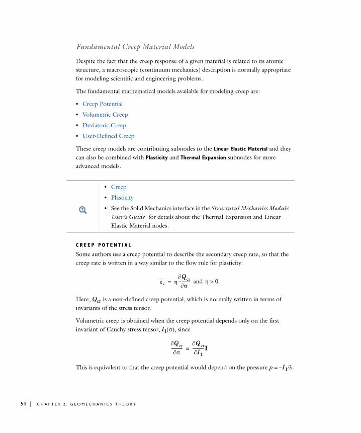
Fundamental Creep Material Models

Despite the fact that the creep response of a given material is related to its atomic structure, a macroscopic (continuum mechanics) description is normally appropriate for modeling scientific and engineering problems.

The fundamental mathematical models available for modeling creep are:

• Creep Potential

• Volumetric Creep

• Deviatoric Creep

• User-Defined Creep

These creep models are contributing subnodes to the Linear Elastic Material and they can also be combined with Plasticity and Thermal Expansion subnodes for more advanced models.

C R E E P PO T E N T I A L

Some authors use a creep potential to describe the secondary creep rate, so that the creep rate is written in a way similar to the flow rule for plasticity:

and

Here, Qcr is a user-defined creep potential, which is normally written in terms of invariants of the stress tensor.

Volumetric creep is obtained when the creep potential depends only on the first invariant of Cauchy stress tensor, I1, since

This is equivalent to that the creep potential would depend on the pressure pI1.

• Creep

• Plasticity

• See the Solid Mechanics interface in the Structural Mechanics Module User’s Guide for details about the Thermal Expansion and Linear Elastic Material nodes.

·c Qcr

-----------= 0

Qcr

-----------QcrI1

-----------I=


When the creep potential depends only on the second deviatoric invariant of Cauchy stress tensor, J2, the deviatoric creep model is obtained since

This is equivalent to that the creep potential would depend on the effective stress e3J2.

When (in SI units) the creep potential, Qcr, is given in units of Pa, the rate multiplier is given in units of 1/s.

VO L U M E T R I C C R E E P

The creep strain rate is calculated by solving the rate equation

so the creep rate tensor is a diagonal tensor, and the trace of the creep rate tensor, the volumetric creep strain rate, equals the user input Fcr

(2-18)

The creep rate, Fcr, usually depends on the first invariant of Cauchy stress I1 or the pressure pI1, in addition to the temperature and other material parameters.

Volumetric creep is not generally used to model creep in metals, but it is commonly used to model creep in soils or other geological materials.

D E V I A T O R I C C R E E P


Here, nD is a deviatoric tensor coaxial to the stress tensor.

The creep rate, Fcr, normally depends on the second deviatoric invariant of the stress J2 or the effective or von Mises (effective) stress e, in addition to the temperature and other material parameters.

The deviatoric tensor nD is defined as

Qcr

-----------QcrJ2-----------dev =

·c13---FcrI=

trace ·c Fcr=

·c FcrnD=

nD 32---dev

e-----------------=


56 | C H A P T E R

The resulting creep strain rate tensor is also deviatoric, since trace (nD)

Given the property

the effective creep strain rate equals the absolute value of the user input Fcr

Deviatoric creep is very popular to model creep in metals and alloys. For example, Norton’s law is a deviatoric creep model.

U S E R - D E F I N E D C R E E P


where Fcr is a user-defined symmetric tensor field.

E N E R G Y D I S S I P A T I O N

Since creep is an inelastic process, the dissipated energy density can be calculated by integrating the creep dissipation rate density (SI unit: W/m3) given by

In case many creep sub-nodes are added to a Linear Elastic Material node, the creep dissipation rate density is calculated from the total creep strain rate tensor .

trace ·c Fcrtrace nD 0= =

nD:nD 32---=

·ce23---·c:

·c Fcr= =

The effective creep strain and the effective creep strain rate are available in the variables solid.ece and solid.ecet.

·c Fcr=

Potential, Volumetric, Deviatoric, or User defined creep do not overwrite each other. These are all contributing nodes to the Linear Elastic Material node.

W·

cdr :·c=

·c


The total energy dissipated by creep in a given volume can be calculated by a volume integration of the dissipated creep energy density Wc (SI unit: J/m3).

Solver Settings for Creep

Creep is a time-dependent phenomenon.

P H Y S I C S I N T E R F A C E S E T T I N G S

In the Model Builder, click the Solid Mechanics node. In the settings window, under Structural Transient Behavior, select Quasi-static to treat the elastic behavior as quasi-static (with no mass effects; that is, no second-order time derivatives for the displacement variables). Selecting this option gives a more efficient solution for problems where the variation in time is slow when compared to the natural frequencies of the system.

S O L V E R S E T T I N G S

When Quasi-static is selected on the physics interface settings window, the automatic solver suggestion changes the method for the Time Stepping from Generalized alpha to BDF.

For a Fully Coupled node (or Segregated node for multiphysics problems), the default Nonlinear method under Method and Termination is Automatic (Newton). To get a faster computation time when the effective strain rate is low or moderate, select Constant

(Newton) as the Nonlinear method instead.

When the Calculate dissipated energy check box is selected, the creep dissipation rate density is available under the variable solid.Wcdr and the dissipated creep energy density under the variable Wc.

• Creep

• Linear Elastic Material in the Structural Mechanics User’s Guide.

In the COMSOL Multiphysics Reference Manual:

• Studies and Solvers

• Fully Coupled and Segregated


58 | C H A P T E R

Re f e r e n c e s f o r t h e Geome chan i c s Modu l e

1. W.F. Chen and E. Mizuno, Nonlinear Analysis in Soil Mechanics: Theory and Implementation (Developments in Geotechnical Engineering), 3rd ed., Elsevier Science, 1990.

2. B. Bresler and K.S. Pister, “Strength of Concrete Under Combined Stresses,” ACI Journal, vol. 551, no. 9, pp. 321–345, 1958.

3. H. Matsuoka and T. Nakai, “Stress-deformation and Strength Characteristics of Soil Under Three Different Principal Stresses,” Proc. JSCE, vol. 232, 1974.

4. H. Matsuoka and T. Nakai, “Relationship Among Tresca, Mises, Mohr-Coulomb, and Matsuoka-Nakai Failure Criteria,” Soils and Foundations, vol. 25, no. 4, pp.123–128, 1985.

5. H.S. Yu, Plasticity and Geotechnics, Springer, 2006.

6. V. Marinos, P. Marinos, and E. Hoek, “The Geological Strength Index: Applications and Limitations,” Bull. Eng. Geol. Environ., vol. 64, pp. 55–65, 2005.

7. J. Jaeger, N. G. Cook, and R. Zimmerman, Fundamentals of Rock Mechanics, 4th ed., Wiley-Blackwell, 2007.

8. G. C. Nayak and O. C. Zienkiewicz, “Convenient Form of Stress Invariants for Plasticity,” J. Struct. Div. ASCE, vol. 98, pp. 949–954, 1972.

9. A.J. Abbo and S.W. Sloan, “A Smooth Hyperbolic Approximation to the Mohr-Coulomb Yield Criterion,” Computers and Structures, vol. 54, no. 3, pp. 427–441, 1995.

10. K.J. Willam and E.P. Warnke, “Constitutive Model for the Triaxial Behavior of Concrete,” IABSE Reports of the Working Commissions, Colloquium (Bergamo): Concrete Structures Subjected to Triaxial Stresses, vol. 19, 1974.

11. B.H.G. Brady and E.T. Brown, Rock Mechanics for Underground Mining, 3rd ed., Springer, 2004.

12. H.A. Taiebat and J.P. Carter, “Flow Rule Effects in the Tresca Model,” Computer and Geotechnics, vol. 35, pp. 500–503, 2008.


13. A. Stankiewicz et al., “Gradient-enhanced Cam-Clay Model in Simulation of Strain Localization in Soil,” Foundations of Civil and Environmental Engineering, no.7, 2006.

14. D.M. Wood, Soil Behaviour and Critical State Soil Mechanics, Cambridge University Press, 2007.

15. D.M. Potts and L. Zadravkovic, Finite Element Analysis in Geothechnical Engineering, Thomas Telford, 1999.

16. W. Tiecheng et al., Stress-strain Relation for Concrete Under Triaxial Loading, 16th ASCE Engineering Mechanics Conference, 2003.

17. W.F. Chen, Plasticity in Reinforced Concrete, McGraw-Hill, 1982.

18. N. Ottosen, “A Failure Criterion for Concrete,” J. Eng. Mech. Division, ASCE, vol. 103, no. 4, pp. 527–535, 1977.

19. N. Ottosen and M. Ristinmaa, The Mechanics of Constitutive Modelling, Elsevier, 2005.

R E F E R E N C E S F O R T H E G E O M E C H A N I C S M O D U L E | 59

60 | C H A P T E R

3

T h e G e o m e c h a n i c s M a t e r i a l s

The Geomechanics Module has materials that are used in combination with the Solid Mechanics interface to account for the plasticity of soils and failure criteria in rocks, concrete, and other materials used in geotechnical applications.

In this chapter:

• Working with the Geomechanics Materials

61

62 | C H A P T E R

Work i n g w i t h t h e Geome chan i c s Ma t e r i a l s

In this section:

• Adding a Material to a Solid Mechanics Interface

• Plasticity

• Soil Plasticity

• Concrete

• Rocks

• Cam-Clay Material

• Creep

Adding a Material to a Solid Mechanics Interface

1 Add a Solid Mechanics interface from the Structural Mechanics branch ( ) when adding a physics interface.

See Geomechanics Theory for background information about these materials.

Creating a New Model in the COMSOL Multiphysics Reference Manual

In general, to add a node, go to the Physics toolbar, no matter what operating system you are using. However, to add subnodes as is the case with those described here, you have to right-click the parent node.

3 : T H E G E O M E C H A N I C S M A T E R I A L S

2 In the Model Builder, right-click the Solid Mechanics node ( ) to add a Cam-Clay

Material subnode. Or right-click a Linear Elastic Material node to add Soil Plasticity, Concrete, and Rocks nodes.

Plasticity

Right-click the Linear Elastic Material node to add the Plasticity subnode. It adds the equations for plasticity in order to make it possible to model elastoplastic materials.

D O M A I N S E L E C T I O N

From the Selection list, choose the domains to add plasticity to a linear elastic material

M O D E L I N P U T S

Use this section to define model inputs such as the temperature field if the material model uses a temperature-dependent material property. If no model inputs are required, this section is empty.

P L A S T I C I T Y M O D E L

Use this section to define the plastic properties of the material.

Plasticity ModelSelect Small plastic strains or Large plastic strains to apply either an additive or multiplicative decomposition between elastic and plastic strains.

Yield Function FThe Yield function F (SI unit: Pa) defines the limit of the elastic regime Fys0.

Except for the settings described in this section, see The Solid Mechanics Interface in the Structural Mechanics Module User’s Guide for details.

Elastoplastic Material Theory

By default, this node inherits the selection from its parent node, and only a selection that is a subset of the parent node’s selection can be used.

W O R K I N G W I T H T H E G E O M E C H A N I C S M A T E R I A L S | 63

64 | C H A P T E R

Select a Yield function F criterion—von Mises stress (the default), Tresca stress, or User

defined:

• The default is von Mises stress with associate plastic potential.

• Select Tresca stress to use a Tresca yield criterion. The plastic potential is nonassociated with the von Mises criterion as flow rule.

• If User defined is selected, enter a different value or expression. Write any expression in terms of the stress tensor variables or its invariants (SI unit: Pa) in the field.

Also select the Plastic potential Q (SI unit: Pa) related to the flow rule—Associated (the default), von Mises, or User defined (nonassociated). If User defined (SI unit: Pa) is selected enter a value in the Q field as required.

Initial Yield StressFor all yield function criteria, the default Initial yield stress ys0 (SI unit: Pa) uses values From material and represents the stress level where plastic deformation starts. Select User defined to enter a different value or expression.

Hardening ModelFor all yield function criteria, select the type of plasticity from the Hardening model list—Isotropic or Perfectly plastic.

• Select Perfectly plastic (ideal plasticity) if it is a material that can undergo plastic deformation without any increase in yield stress.

• If Isotropic is selected, also choose an Isotropic hardening model—Use tangent data or Use hardening function data.

- If Use tangent data is selected, the default Isotropic tangent modulus ETiso (SI unit: Pa) uses values From material (if it exists) or User defined, and so the yield level ys is modified as hardening occurs. The Young’s modulus E is taken from


the elastic material properties. The yield level ys is related to the effective plastic strain pe as

This is a linear isotropic hardening model, so the yield level increases proportionally to the effective plastic strain pe.

- If Use hardening function data is selected, the Hardening functionh(pe) (SI unit: Pa) uses values From material (if it exists) or User defined, the yield level ys is modified as

This definition implies that the hardening function must be zero at zero plastic strain. In other words, ysys0 whenpe0. With this option it is possible to fit nonlinear isotropic hardening curves depending on stress level, temperature or other variables.

Soil Plasticity

Right-click the Linear Elastic Material node to add a Soil Plasticity subnode. The Soil

Plasticity node adds the equations for linear elasticity and plasticity and the interface for defining the elastic material properties and yield surface. The yield criteria are described in the theory section:

• Drucker-Prager Criterion

• Mohr-Coulomb Criterion

• Matsuoka-Nakai Criterion

• Lade-Duncan Criterion


From the Selection list, choose the domains to compute the displacements, stresses, and strains.


Define model inputs, for example, the temperature field of the material uses a temperature-dependent material property. If no model inputs are required, this section is empty.

ys ys0ETiso

1ETiso

E--------------–

------------------------pe+=

ys ys0 h pe +=


66 | C H A P T E R

S O I L P L A S T I C I T Y

Select a Yield criterion—Drucker-Prager, Mohr-Coulomb, Matsuoka-Nakai, or Lade-Duncan.

Drucker-PragerIf required, select the Match to Mohr-Coulomb criterion check box (see Mohr-Coulomb Criterion). If this check box is selected, the default values for Cohesion c (SI unit: Pa) and the Angle of internal friction (SI unit: rad) are taken From material. If User defined is selected, then enter other values or expressions.

If required, select the Use dilatation angle in plastic potential check box. If this check box is selected, then enter a value or expression for the Dilatation angle (SI unit: rad). Alternatively, select From material. The dilatation angle replaces the angle of internal friction when defining the plastic potential.

If the Match to Mohr-Coulomb criterion check box is not selected, then the default Drucker-Prager alpha coefficient (dimensionless) and Drucker-Prager k coefficient k (SI unit: Pa) are taken From material. Select User defined to enter other values or expressions.

If required, select the Include elliptic cap check box (see Elliptic Cap). Enter values or expressions for the semi-axes of the Elliptic cap parameter Pa and Elliptic cap parameter Pb (SI unit: Pa).

Mohr-CoulombThe default Angle of internal friction (SI unit: rad) and Cohesion c (SI unit: Pa) are taken From material. Select User defined to enter other values or expressions.

If required, select the Use dilatation angle in plastic potential check box. If this check box is selected, then enter a value or expression for the Dilatation angle (SI unit: rad). Alternatively, select From material. The dilatation angle replaces the angle of internal friction when defining the plastic potential.

Under Plastic potential select either Drucker-Prager matched at compressive meridian, Drucker-Prager matched at tensile meridian, or Associated.

If required, select the Include elliptic cap check box (see Elliptic Cap). Enter values or expressions for the semi-axes of the Elliptic cap parameter Pa and Elliptic cap parameter Pb (SI unit: Pa).


Matsuoka-NakaiIf required, select the Match to Mohr-Coulomb criterion check box. If this check box is selected, the default Angle of internal friction (SI unit: rad) is taken From material. Select User defined to enter other values or expressions.

If the Match to Mohr-Coulomb criterion check box is not selected, then the default Matsuoka-Nakai mu coefficient (dimensionless) is taken From material. Select User

defined to enter other values or expressions.

Lade-DuncanIf required, select the Match to Mohr-Coulomb criterion check box. If this check box is selected, then enter a value or expression for the Angle of internal friction (SI unit: rad). Alternatively, select From material.

If the Match to Mohr-Coulomb criterion check box is not selected, then the default Lade-Duncan k coefficient k(dimensionless) is taken From material. Select User defined

to enter other values or expressions.

TE N S I O N C U T - O F F

If required, select the Include tension cut-off check box (see Tension Cut-Off). Enter a value or expression for the Max tensile stress t (SI unit: N/m2). Use this to constrain the soil plasticity model with an extra yield surface, which limits the maximum principal stress.

Concrete

Right-click the Linear Elastic Material node to add a Concrete subnode. The Concrete

node adds the equations for linear elasticity, and the interface for defining the elastic material properties and failure surface. The failure criteria are described in the theory section:

• Bresler-Pister Criterion

• Willam-Warnke Criterion

• Deep Excavation: model library path Geomechanics_Module/Soil_Models/deep_excavation

• Flexible and Smooth Strip Footing on Stratum of Clay: model library path Geomechanics_Module/Soil_Models/flexible_footing


68 | C H A P T E R

• Ottosen Criterion

C O N C R E T E M O D E L

Select a Concrete criterion—Bresler-Pister, Willam-Warnke, or Ottosen.

Bresler-PisterThe defaults for the Uniaxial tensile strength t, Uniaxial compressive strength c, and Biaxial compressive strength b (SI units: Pa) are taken From material. Select User


Willam-WarnkeThe defaults for the Uniaxial tensile strength t, Uniaxial compressive strengthc, and Biaxial compressive strength b (SI units: Pa) are taken From material. Select User


OttosenThe defaults for the Uniaxial tensile strengthc (SI unit: Pa), Ottosen’s parameters a and b (dimensionless), Size factor k1 (dimensionless), and Shape factor k2 (dimensionless) are taken From material. Select User defined to enter other values or expressions.

TE N S I O N C U T - O F F

If required, select the Include tension cut-off check box (see Tension Cut-Off). Enter a value or expression for the Max tensile stress t (SI unit: N/m2). Use this to constraint the concrete model with an extra yield surface, which limits the maximum principal stress.

The settings for Domain Selection, Model Inputs, and Linear Elastic Model are the same as for the Soil Plasticity.


Rocks

Right-click the Linear Elastic Material node to add a Rocks subnode. The Rocks node adds the equations for linear elasticity, and the interface for defining the elastic material properties and failure surface. The failure criterion are described in the theory section:

• Original Hoek-Brown Criterion

• Generalized Hoek-Brown Criterion

R O C K M O D E L

Select a Rock criterion—Original Hoek-Brown or Generalized Hoek-Brown.

Original Hoek-BrownThe defaults for the Uniaxial compressive strengthc (SI unit: Pa), Hoek-Brown m

parameter m (dimensionless), and Hoek-Brown s parameter s (dimensionless) are taken From material. Select User defined to enter other values or expressions.

Generalized Hoek-BrownThe defaults for the Uniaxial compressive strengthc (SI unit: Pa), Geological strength

index GSI (dimensionless), Disturbance factor D (dimensionless), and Intact rock

parameter (dimensionless) mi are taken From material. Select User defined to enter other values or expressions.

Cam-Clay Material

The Cam-Clay Material node adds the equations and interface for defining the material properties for the modified Cam-clay material (see Theory for the Cam-Clay Material). Right-click to add the Thermal Expansion and Initial Stress and Strain subnodes.


From the Selection list, choose the domains to compute the displacements, stresses, and strains.

The settings for Domain Selection, Model Inputs, and Linear Elastic Model are the same as for the Soil Plasticity.


70 | C H A P T E R


The Pore fluid pressure pfluid (SI unit: Pa) is user-defined by default. The default value is 1 atm, but you can change it to another value or expression for the pore fluid pressure.

C A M - C L A Y M A T E R I A L

To use a mixed formulation by adding the negative mean pressure as an extra dependent variable to solve for, select the Nearly incompressible material check box.

From the Specify list, define the elastic properties either in terms of Poisson’s ratio or Shear modulus.

The defaults for the Poisson’s ratio (dimensionless) or the Shear modulus G (SI unit: Pa), Density (SI unit: kg/m3), Cam-Clay M parameter M (dimensionless), Swelling index (dimensionless), Compression index (dimensionless), and Void ratio

at reference pressure N (dimensionless) are taken From material. Select User defined for any of these parameters to enter other values or expressions.

Enter a value or expression for the Reference pressure for the parameter N prefN (SI unit: Pa), the Initial void ratio e0,and the Initial consolidation pressure pc0 (SI unit: Pa).

G E O M E T R I C N O N L I N E A R I T Y

Select the Force linear strains check box as required.

For the Cam-Clay M parameter you can alternatively select Match to

Mohr-Coulomb criterion which then matches the slope of the virgin consolidation line to the Angle of internal friction. Then select the Angle

of internal friction (SI unit: rad) as From material (the default) or User

defined.

Geometric Nonlinearity Theory for the Solid Mechanics Interface in the Structural Mechanics Module User’s Guide

Isotropic Compression: model library path Geomechanics_Module/Verification_Models/isotropic_compression


Creep

Right-click the Linear Elastic Material node to add a Creep subnode to a model. Use the Creep node to define the material model.


From the Selection list, choose the domains to define.


From the Temperature T (SI unit: K) list, select an existing temperature variable from a heat transfer interface (for example, Temperature (ht/sol1)), if any temperature variables exist, or select User defined to enter a value or expression for the temperature (the default is 293.15 K).

C O O R D I N A T E S Y S T E M S E L E C T I O N

The Global coordinate system is selected by default. The Coordinate system list contains any additional coordinate systems that the model includes.

C R E E P D A T A

Select a Material model—Potential, Volumetric, Deviatoric, or User defined.

• If Potential is selected, enter the Rate multiplier (SI unit: 1/s) (the default is 0 (1/s)) and the Creep potential Qcr (SI unit: N/m2) (the default is 0 N/m2).

Thermal Expansion and Initial Stress and Strain in the Structural Mechanics Module User’s Guide

See Creep and Viscoplasticity for background theory about this feature.


72 | C H A P T E R

• If Deviatoric or Volumetric is selected, enter the Creep rate Fcr (SI unit: 1/s). The default is 0 1/s.

• If User defined is selected, enter each element for the symmetric Creep rate tensor Fcr (SI unit: 1/s). The defaults are 0 1/s.

The Energy Dissipation section is also available on the Linear Elastic Material settings window as an advanced feature (to display the section, click the Show button ( ) and select Advanced Physics Options).

See Energy Dissipation in the theory section for more information about this option.


I n d e x

A absolute values 37

alpha coefficient 66

angle of internal friction 20, 26, 66

associated flow rule 43

B back stress 48

biaxial compression 34

biaxial data 36

biaxial tension 68

Bresler-Pister criterion 33

C calcite 37

Cam-Clay material (node) 69

Cam-clay model 28

carbonate rocks 37

Cauchy stress tensor 13

Cayley-Hamilton theorem 13

ceramics 34

circle, Mohr 20

clays 19

cohesion 20, 66

cohesionless soils 26

cohesive-frictional materials 34

complementarity 43

compressive meridians 14, 21, 34–35

compressive stresses 12

concrete 33, 35

concrete (node) 67

consistency parameter 42

continuum mechanics 12

creep (node) 71

creep dissipation rate density 56

creep strain rate 52

crystal cleavage 37

D deviatoric creep 56

deviatoric stress 13, 17

dissipated energy density 56

disturbance factor 39

documentation 7

dolomite 37

Drucker-Prager criterion 22

ductile materials 19

E effective creep strain rate 56

effective plastic strain rate 44

effective stress tensor 38

elastic deformation gradient 41

elastic Green-Lagrange strain tensor 41

elastic right Cauchy-Green tensor 42

elastic volumetric strain variable 31

elastoplastic materials 16, 34

elliptic cap 24

elplastic 43, 50

emailing COMSOL 9

F failure surfaces 16

flow rule 42

fluid pore pressure 25

friction, angle 20, 26, 66

frictionless materials 21, 23

G Gauss points 43, 50

generalized Hoek-Brown criterion 38

geological strength index (GSI) 38

H Haigh–Westergaard coordinates 14

hardening function data 47

hardening models

plasticity node settings 64

theory 46

Hencky plastic strain 50

hexagonal prism 18

Hoek-Brown criterion 37

hydrostatic axis 14

hydrostatic pressure 12, 20

hydrostatic stress 26

I N D E X | 73

74 | I N D E X

I ideal plasticity 46

initial yield stress 47

Internet resources 6

isotropic hardening 46

isotropic materials 17

isotropic plasticity 43

isotropic rocks 38

K k coefficient 67

kinematic hardening 47

knowledge base, COMSOL 9

Kuhn-Tucker conditions 43

L Lade-Duncan criterion 26

large plastic strain 41

Lie derivative 49

limestone 37

Lode angle 14

Hoek-Brown criterion 38

Mohr-Coulomb criterion 21

Tresca criterion 18

Willam-Warnke criterion 34

logarithmic plastic strain 50

M marble 37

Matsuoka-Nakai criterion 25

meridians, tensile and compressive 14,

21, 34–35

metal plasticity 44

metals 19, 22

mixed formulation 70

mobilized planes 25

Model Libraries window 8

model library examples

Cam-Clay material 70

soil plasticity 67

modified Cam-clay model 28

modified Mohr-Coulomb criterion 27

Mohr-Coulomb criterion 20

MPH-files 8

mu coefficient 67

multiaxial stress states 33

N nearly incompressible material 70

non-associated flow rule 43

O octahedral normal stress 33

octahedral plane 15

Ottosen criterion 35

over-consolidation pressure 29

P perfectly elastoplastic materials 17

perfectly plastic hardening 46

plastic deformation gradient 42

plastic element 43, 50

plastic flow rule 50

plastic Green-Lagrange strain 42

plastic multiplier 42

plastic potential 42

plastic right Cauchy-Green tensor 42

plasticity (node) 63

plasticity models 63

plasticity, theory 12

Prager’s hardening rule 48

primary creep 52

principal stresses 15

R rate independent plasticity 42

rate of strain tensor 49

rock mass 39

rock types 37

rock yield criteria 20

rocks 37

rocks (node) 69

S saturated cohesive soils 19

secondary creep 53

shape factors 36

shear stresses 14, 20, 33

sign convention 12

size factors 36

small plastic strain 40

soil deformation theory 30

soil plasticity 14

soil plasticity (node) 65

soil yield criteria 20

spatially mobilized planes (STP) 25

steady-state creep 53

stress invariants 13

T tangent data 46

tangent modulus 47

technical support, COMSOL 9

tensile meridian 14

tensile meridians 21–22, 26, 34–35

tensile normal strains and stresses 12

tension cut-off 27

tertiary creep 53

transient creep 52

Tresca effective stress variable 18

Tresca stress 45

Tresca yield criterion 18

triaxial conditions 34

triaxial data 36

U undrained shear strength 18

uniaxial compression 36–37

uniaxial compressive strength 33

uniaxial tension 17, 68

user community, COMSOL 9

V variables

effective creep strain 56

effective plastic strain 45, 47

elastic volumetric strain 31

Tresca effective stress 18

volumetric plastic strain 29, 45

volumetric creep strain rate 55

volumetric plastic strain rate 44

volumetric plastic strain variable 29

von Mises criterion 17, 44

von Mises stress 45

W web sites, COMSOL 9

Willam-Warnke criterion 34

Y yield function 45

yield functions 17, 20

yield stress levels 64

yield surface 43

yield surfaces 16, 22

I N D E X | 75

76 | I N D E X

the geomechanics module user’s guide · 5 1 introduction w elcome to the geomechanics module...

Documents