the geometry of hilbert functions introductionjmiglior/hilb.pdf · the geometry of hilbert...

THE GEOMETRY OF HILBERT FUNCTIONS

JUAN C. MIGLIORE

1. Introduction

The title of this paper, “The geometry of Hilbert functions,” mightbetter be suited for a multi-volume treatise than for a single shortarticle. Indeed, a large part of the beauty of, and interest in, Hilbertfunctions derives from their ubiquity in all of commutative algebra andalgebraic geometry, and the unexpected information that they can give,very much of it expressible in a geometric way. Most of this paper isdevoted to describing just one small facet of this theory, which connectsresults of Davis (e.g. [Davis]) in the 1980’s, of Bigatti, Geramita andmyself (cf. [Bigatti-Geramita-Migliore]) in the 1990’s, and of Ahn andmyself (cf. [Ahn-Migliore]) very recently. On the other hand, we havean alphabet soup of topics that play a role here: UPP, WLP, SLP,ACM at the very least. It is interesting to see the ways in which theseproperties interact, and we also try to illustrate some aspects of this.

There are almost as many different notations for Hilbert functionsas there are papers on the subject. We will use the following notation.If I is a homogeneous ideal in a polynomial ring R, we write

hR/I(t) := dim(R/I)t.

If I is a saturated ideal defining a subscheme V of Pn then we also

write this function as hV (t) or hR/IV(t).

So where is the geometry? Of course dimRt =(

t+nn

), so the in-

formation provided by the Hilbert function is equivalent to giving thedimension of the degree t component of I. This dimension is one morethan the dimension of the linear system of hypersurfaces of degree tdefined by It (since this latter dimension is projective). What is thebase locus of this linear system? Of course V is contained in this baselocus, but it may contain more. The results in this paper (e.g. Theo-rem 5.3, Theorem 5.4, Theorem 6.2 and Theorem 6.5) can be viewedas describing the dimension, irreducibility and reducedness of this baselocus, based on information about the Hilbert function, and other basicproperties, of V . We will see that under some situations, just knowingthe dimension of this linear system in two consecutive degrees can force

1

2 JUAN C. MIGLIORE

the base locus to contain a hypersurface, or anything smaller. (We willconcentrate on the curve case.)

An important starting point for us (and indeed for almost any dis-cussion of Hilbert functions of standard graded algebras) is Macaulay’stheorem bounding the growth of the Hilbert function. Once we havethis, we need Gotzmann’s results about what happens when Macaulay’sbound is achieved. These are both discussed in Section 2, as are severalother results related to these.

In Section 3 we recall the notions of the Uniform Position Property(UPP) and the Weak Lefschetz Property (WLP) and some of theirconnections. Subsequent sections, especially Section 6, continue thediscussion of UPP. WLP, while often less visible, lurks in the back-ground of many of the results and computations of this paper, and infact is an important object of study. We include a short discussion ofthe behavior of WLP in families of points in Section 3, including a newexample (Example 3.4) showing how, for fixed Hilbert function, WLPcan hold in one component of the postulation Hilbert scheme and nothold in another. See also Theorem 5.6.

The focus in this article is the situation where the first difference ofthe Hilbert function of a set of points, Z, in projective space P

n attainsthe same value in two consecutive degrees: ∆hZ(d) = ∆hZ(d+ 1) = s.Depending on the relation between d, s and certain invariants of Z,we will get geometric consequences for the base locus. In Section 4 wedescribe these relations, setting the stage for the main results.

These main results are given in Sections 5 and 6. Here we see that un-der certain assumptions on d, the condition ∆hZ(d) = ∆hZ(d+ 1) = sguarantees that the base locus of the linear system |Id| is a curve of de-gree s. This comes from work in [Davis], [Bigatti-Geramita-Migliore]and [Ahn-Migliore]. Other results follow as well. What is surpris-ing here is that the central condition of [Ahn-Migliore], namely thatd > r2(R/IZ) (see Section 2 for the definition), is much weaker thanthe central assumption of the comparable results in [Bigatti-Geramita-Migliore], namely d ≥ s, but the results are very similar. Section 5focuses on the general results, while Section 6 turns to the question ofwhat can be said about this base locus when the points have UPP.

There are some differences in the results of [Bigatti-Geramita-Migliore] and [Ahn-Migliore] as a result of the differences in these as-sumptions. Section 7 studies these, and gives examples to show thatthey are not accidental omissions. Some very surprising behavior isexhibited here.

I am grateful to Irena Peeva for asking me to write this paper, whichI enjoyed doing. In part it is a greatly expanded version of a talk

THE GEOMETRY OF HILBERT FUNCTIONS 3

that I gave in the Algebraic Geometry seminar at Queen’s Univer-sity in the fall of 2004, and I am grateful to Mike Roth and to GregSmith for their kind invitation. I would like to thank Jeaman Ahn,Chris Francisco, Hal Schenck and especially Tony Iarrobino for helpfulcomments. And of course I am most grateful to my co-authors AnnaBigatti and Tony Geramita ([Bigatti-Geramita-Migliore]) and JeamanAhn ([Ahn-Migliore]) for their insights and for the enjoyable times thatwe spent in our collaboration. During the writing of this paper, andsome of the work described here, I was sponsored by the National Se-curity Agency (USA) under Grant Number MDA904-03-1-0071.

2. Maximal growth of the Hilbert function

We first collect the notation that we will use throughout this paper.Let k be a field of characteristic zero and let R = k[x1, . . . , xn].

Definition 2.1. Let Z ⊂ Pn−1 be any closed subscheme with defining

(saturated) ideal I = IZ .

(a) The Hilbert function of Z is the function

hZ(t) = dim(R/IZ)t

We also may write hR/I(t) for this function. If A is Artinian thenwe write

hA(t) = dimAt

for its Hilbert function.(b) We say that Z is arithmetically Cohen-Macaulay (ACM) if the

coordinate ring R/IZ is a Cohen-Macaulay ring. Note that if Z isa zero-dimensional scheme then it is automatically ACM.

If F is a homogeneous polynomial, by abuse of notation we will alsodenote by F the hypersurface of P

n−1 defined by F .

Definition 2.2. For a homogeneous ideal I we define

α = min{t | It �= 0},

i.e. α is the initial degree of I.

If A = R/I is a standard graded k-algebra, then there is a famousbound, due to Macaulay (cf. [Macaulay]), that describes the maximumpossible growth of the Hilbert function of A from any degree to thenext. To give this bound, we need a little preparation.

4 JUAN C. MIGLIORE

Definition 2.3. The i-binomial expansion of the integer c (i, c > 0) isthe unique expression

c =

(mi

i

)+

(mi−1

i− 1

)+ · · · +

(mj

j

),

where mi > mi−1 > · · · > mj ≥ j ≥ 1.

Note that the assertion that this representation is unique is some-thing that has to be checked!

Definition 2.4. If c ∈ Z (c > 0) has i-binomial expansion as in Defi-nition 2.3, then we set

c〈i〉 =

(mi + 1

i+ 1

)+

(mi−1 + 1

i

)+ · · · +

(mj + 1

j + 1

).

Note that this defines a collection of functions 〈i〉 : Z → Z.

For example, the 5-binomial expansion of 76 is

76 =

(8

5

)+

(6

4

)+

(4

3

)+

(2

2

),

so

76〈5〉 =

(9

6

)+

(7

5

)+

(5

4

)+

(3

3

)= 111.

Definition 2.5. A sequence of non-negative integers {ci : i ≥ 0} iscalled an O-sequence if

c0 = 1 and ci+1 ≤ c〈i〉i ,

for all i. An O-sequence is said to have maximal growth from degree i

to degree i+ 1 if ci+1 = c〈i〉i .

The importance of the binomial expansions described above becomesapparent from the following beautiful theorem of Macaulay:

Theorem 2.6 ([Macaulay]). The following are equivalent:

(i) {ci : i ≥ 0} is an O-sequence;(ii) {ci : i ≥ 0} is the Hilbert function of a standard graded k-algebra.

In other words, a sequence of non-negative integers is the Hilbert func-tion of a standard graded k-algebra if and only if the growth from anydegree to the next is bounded as above. Remember that the Hilbert


function is eventually equal to the Hilbert polynomial, but until that

point, anything is allowed as long as we maintain ci+1 ≤ c〈i〉i .

One can ask when such a sequence is the Hilbert function of a reducedk-algebra. This was answered by Geramita, Maroscia and Roberts (cf.[Geramita-Maroscia-Roberts]), by introducing the first difference of theHilbert function.

Definition 2.7. Given a sequence of non-negative integers c ={ci : i ≥ 0}, the first difference of this sequence is the sequence∆c := {bi} defined by bi = ci − ci−1 for all i. (We make the con-vention that c−1 = 0, so b0 = c0 = 1.) We say that c is a differentiableO-sequence if ∆c is again an O-sequence. By taking successive first

differences, we inductively define the k-th difference ∆kc.

Remark 2.8. An important fact to remember is that if Z is a zero-dimensional scheme with Artinian reduction A then

hA(t) = ∆hZ(t) for all t.

It follows that (∆hZ(t) : t ≥ 0) is a finite sequence of positive integers,called the h-vector of Z. Similarly, if V is ACM of dimension d with

Artinian reduction A then hA(t) = ∆d+1hV (t) for all t.

The following is the theorem of Geramita, Maroscia and Robertsmentioned above. It guarantees the existence of a reduced subschemeof P

n−1 with given Hilbert function (remember that R = k[x1, . . . , xn]),under a simple hypothesis on the Hilbert function.

Theorem 2.9 ([Geramita-Maroscia-Roberts]). Let c = {ci} be a se-quence of non-negative integers, with c1 = n. Then c is the Hilbertfunction of a standard graded k-algebra R/I, with I radical, if andonly if c is a differentiable O-sequence.

Note that if I is any saturated ideal (reduced or otherwise), and if L isa general linear form, then we have [I : L] ∼= I(−1) as graded modules.It follows that L induces an injection ×L : ((R/I)(−1))t → (R/I)t,i.e. R/I has depth at least 1. Hence the first difference of the Hilbertfunction of R/I is the Hilbert function of R/(I, L), again a standardgraded k-algebra, so the Hilbert function of R/I is a differentiable O-sequence. This shows that Theorem 2.9 would also be true if “radical”were replaced by “saturated” (since if a radical ideal can be constructedfor a given differentiable O-sequence, this ideal is also saturated). Thereal heart of Theorem 2.9 is that any such sequence can be achievedby a radical ideal.

6 JUAN C. MIGLIORE

Example 2.10. We should stress that Theorem 2.9 guarantees theexistence of a reduced (even non-degenerate) subscheme of P

n, but itdoes not guarantee that what we get will be equidimensional. It alsodoes not say anything about higher differences. (Note that even if I issaturated, this is not necessarily true of (I, L).) We give two examples.

1. Let I = (x1, x2) in k[x0, x1, x2, x3], so I defines a line, λ, in P3.

Let F be a homogeneous polynomial of degree 3, non-singularalong λ. Let J = (I2, F ). Then J is the saturated ideal of a non-reduced subscheme of degree 2 and genus −2 (cf. [MIgliore2]).Its Hilbert function is the sequence 1, 4, 7, 9, 11, . . . (with Hilbertpolynomial 2t+ 3). The smallest genus for a reduced equidimen-sional subscheme of degree 2 is −1 (two skew lines), so this Hilbertfunction does not exist among reduced, equidimensional curves inP

3. However, adding points reduces the genus while not affectingthe degree, and in fact this Hilbert function occurs for the unionof two skew lines and one point, which is indeed reduced.

2. Consider the sequence c = 1, 4, 10, 17, 26, 35, . . . (with Hilbertpolynomial 9t − 11 + 1, so it corresponds to a curve of degree9 and arithmetic genus 11). Its first difference is 1, 3, 6, 7, 9, 9, . . . ,which is again an O-sequence, so c is a differentiable O-sequence.However, the second difference is 1, 2, 3, 1, 2 which is not an O-sequence. Theorem 2.9 guarantees the existence of a reducedcurve with Hilbert function c, and indeed it can be achieved bythe union C1∪C2∪P1∪P2, where C1 is a plane curve of degree 3,C2 is a plane curve of degree 6 not in the plane of C1, C1 and C2

meet in 3 points, P1 is a generally chosen point in P3, and P2 is a

generally chosen point in the plane of C1.

One sees that finding the reduced subscheme of Theorem 2.9 can be atricky matter!

If h = {ci : i ≥ 0} is an O-sequence, Theorem 2.6 guarantees that his the Hilbert function of a standard graded k-algebra, say R/I. Thefollowing striking result of Gotzmann says what happens if we have

maximal growth (see Definition 2.5), i.e. if the equality cd+1 = c〈d〉d

holds. Let I be the ideal generated by the components of I of degree

≤ d, so that Ii = Ii for all i ≤ d. We also sometimes write I = 〈I≤d〉.

Theorem 2.11 ([Gotzmann], [Green1]). Let h = {ci : i ≥ 0} be the

Hilbert function of R/I, and suppose that cd =(

md

d

)+

(md−1

d−1

)+· · ·+

(mj

j

)is the d-binomial expansion of cd. Assume that cd+1 = c

〈d〉d . Then for


any l ≥ 1 we have

cd+l =

(md + l

d+ l

)+

(md−1 + l

d− 1 + l

)+ · · · +

(mj + l

j + l

).

In particular, the Hilbert polynomial pR/I(x) agrees with the Hilbert

function hR/I(x) in all degrees ≥ d. It can be written as

pR/I(x) =

(x+md − d

md − d

)+

(x+md−1 − d

md−1 − (d− 1)

)+ · · · +

(x+mj − d

mj − j

),

where md − d ≥ md−1 − (d− 1) ≤ · · · ≤ mj − j.

Remark 2.12. Theorem 2.11 is also known as the Gotzmann Persis-tence Theorem. Since pR/I(x) has degree md − d, this means that the

Krull dimension dimR/I = md − d + 1, and I defines a subscheme ofdimension md − d. Its degree can also easily be computed by checking

the leading coefficient. Gotzmann also shows that I has regularity ≤ dand agrees with its saturation in degrees ≥ d.

Remark 2.13. An excellent reference for the Gotzmann PersistenceTheorem and related results is section 4.3 of [Bruns-Herzog] (note thatthis is the revised edition; this material does not appear in the originalbook). A much more detailed and comprehensive expository treatmentthan that given here can be found in [Iarrobino-Kanev], Appendix C(written by A. Iarrobino and S. Kleiman). This includes a detaileddescription of the associated Hilbert scheme.

Much of the work described in this paper revolves around the follow-ing idea. If I is a saturated homogeneous ideal and L is a general linearform, then reducing modulo L gives a new ideal, J , in S = R/(L). Sup-pose that S/J has maximal growth from degree d to degree d+1. Thisdoes not necessarily imply that R/I has maximal growth at that spot(see also Remark 4.5). Then what information can we get about I ifwe know that R/J has maximal growth? As a first step we have thefollowing result from [Bigatti-Geramita-Migliore]. We have noted inRemark 2.12 that maximal growth of J implies something about thesaturation and regularity of J , thanks to Gotzmann, but we now showthat it also says something about the saturation and regularity of 〈I≤d〉.

Proposition 2.14. ([Bigatti-Geramita-Migliore] Lemma 1.4, Proposi-tion 1.6) Let I ⊂ R be a saturated ideal. Let L be a general linear form,

and let J = (I,L)(L)

⊂ S = R/(L). Suppose that S/J has maximal growth

8 JUAN C. MIGLIORE

from degree d to degree d + 1. Let I = 〈I≤d〉 as above. Let Isat be the

saturation of I. Then I = Isat, i.e. I is a saturated ideal. Furthermore,

I is d-regular.

Remark 2.15. Again, Proposition 2.14 differs from the Gotzmann re-sults (cf. Theorem 2.11, Remark 2.12) in that S/J is assumed to havemaximal growth, but we conclude something about I. But even beyondthis, there is another difference between Proposition 2.14 and the partof Gotzmann’s work that we have presented (referring to the sourcesmentioned in Remark 2.13 for a more complete exposition); indeed,in Theorem 2.11 and Remark 2.12 we only conclude that the ideal inquestion agrees with its saturation in degree d and beyond, while herewe make a conclusion about the whole ideal. (The price is that we haveto assume that I itself is saturated to begin with, although this doesnot necessarily hold for J .)

Also, the maximal growth assumption for S/J is necessary. Forinstance, let I be the saturated ideal of a set, Z, of sixteen gen-eral points in P

3. Then I has four generators in degree 3 and threegenerators in degree 4. The four generators in degree 3 do define Zscheme-theoretically, but this is not enough. One can check (e.g. using

macaulay [Bayer-Stillman]) that if I = 〈I≤3〉, then Isat = I �= 〈I≤3〉 =

I. Furthermore, I is 5-regular and I itself is 4-regular, and neither is3-regular. And indeed, the Hilbert function of S/J is 1, 3, 6, 6, 0, so wedo not have maximal growth of S/J from degree 3 to degree 4.

Despite this, the results in [Ahn-Migliore] show that statements alongthe lines of Proposition 2.14 can be obtained even weakening the max-imal growth assumption.

3. UPP and WLP

A very important property of (many) reduced sets of points in pro-jective space is the following:

Definition 3.1. A reduced set of points Z ⊂ Pn−1 has the Uniform

Position Property (UPP) if, for any t ≤ |Z|, all subsets of t points havethe same Hilbert function, which necessarily is the truncated Hilbertfunction.

The last comment follows from the fact that it was also shown in[Geramita-Maroscia-Roberts] that given any reduced set Z of, say, dpoints with known Hilbert function, and truncating this function atany value k < d, there is a subset X of Z consisting of k points whose


Hilbert function is this truncated function. Hence if Z has UPP, thenall subsets have this truncated Hilbert function.

While it is known that the general hyperplane section of an irre-ducible curve has UPP (cf. [Harris-Eisenbud]), at least in character-istic zero, much remains open. An important open question is to de-termine all possible Hilbert functions of sets of points in projectivespace with UPP. It is known in P

2 but it is open even in P3. See

[Geramita-Migliore] for a discussion of several of the many papers that

have contributed to this question for P2.

For any given Hilbert function, there may or may not be a set ofpoints with UPP having that Hilbert function. One of the contributionsof the papers discussed here is toward showing some conditions on theHilbert function that prohibit the existence of points with UPP havingthat function. If there is a set of points with UPP having a given Hilbertfunction, somehow “most” sets of points with that Hilbert functionhave UPP: consider the postulation Hilbert scheme parameterizing setsof points with that Hilbert function; then in the component containingthe given set of points, there is an open subset corresponding to pointswith UPP. (We make this more precise in the discussion about WLPbelow.)

Another important property is the following.

Definition 3.2. An Artinian algebra A has the Weak Lefschetz Prop-erty (WLP) if, for a general linear form L, the map ×L : At → At+1

has maximal rank, for all t. We say that A has the Strong LefschetzProperty (SLP) if for every d, and for a general form F of degree d,the map ×F : At → At+d has maximal rank, for all t. If Z is a setof points, we sometimes say that Z has WLP or SLP if its generalArtinian reduction does

Remark 3.3. We have the following comments about WLP and SLP:

1. The statement that SLP holds for an ideal of any number ofgeneral forms is equivalent to the well-known Froberg conjec-ture. See [Anick], [Migliore-Miro-Roig1], [Migliore-Miro-Roig2],[Migliore-Miro-Roig-Nagel].

2. Every Artinian complete intersection in k[x1, x2, x3] has WLP (cf.[Harima-Migliore-Nagel-Watanabe]). It is also known that SLP(and hence WLP) holds for every ideal in k[x1, x2] (cf. [Iarrobino1],[Harima-Migliore-Nagel-Watanabe]), and it (and hence Froberg’sconjecture) holds for an ideal of general forms in k[x1, x2, x3] (cf.[Anick]).

10 JUAN C. MIGLIORE

We now begin a short digression about the behavior of WLP in fam-ilies of reduced zero-dimensional schemes. Fix a Hilbert function, H,that corresponds to a zero-dimensional scheme, and consider the h-vector, h = (a0, a1, a2, . . . , as), associated to that Hilbert function (i.e.

its first difference ∆H – cf. Remark 2.8). Let d =∑

i ai be the degree ofthe zero-dimensional scheme. Consider the postulation Hilbert scheme,

Hh := HilbH(Pn), parameterizing zero-dimensional schemes in Pn with

Hilbert function H (inside the punctual Hilbert scheme, Hilbd(Pn), ofall zero-dimensional schemes in P

n with the given degree). It is known

that the closure, Hh, of Hh may have several irreducible components –

see for instance Richert (cf. [Richert], and use Hartshorne’s lifting pro-cedure, cf. [Hartshorne], [Migliore-Nagel], on the Artinian monomialideals that Richert gives), Ragusa-Zappala (cf. [Ragusa-Zappala]) orKleppe (cf. [Kleppe], Remark 27). We will consider only those compo-

nents of Hh for which the general element is reduced.One can show that, like UPP, WLP is an open condition in the

sense that in any component of Hh, an open subset (possibly empty)corresponds to zero-dimensional schemes with WLP. We will now givean example that answers (positively) the following question. Namely,does there exist a Hilbert function with h-vector h, and components

H1 and H2 of the corresponding Hh, for which

• h = (a0, a1, a2, . . . , as) is unimodal, and in fact satisfies

a0 < a1 < a2 · · · < at ≥ at+1 ≥ · · · ≥ as.(1)

for some t (this is a technical necessity for WLP– cf. [Harima-Migliore-Nagel-Watanabe], Remark 3.3);

• the general element of H1 corresponds to a reduced, zero-dimen-sional scheme with WLP;

• no element of H2 corresponds to a zero-dimensional scheme withWLP (i.e. the open subset referred to above is empty)?

The following example answers this question.

Example 3.4. We will give an example of ideals I1 and I2 of reducedzero-dimensional schemes in P

3, both with h-vector

h = (1, 3, 6, 9, 11, 11, 11),

such that the Artinian reduction of R/I1 has WLP and the Artinianreduction of R/I2 does not. Furthermore, the Betti diagrams for R/I1and R/I2 are (respectively)


total: 1 14 24 11 total: 1 14 25 12-------------------------------- --------------------------------

0: 1 - - - 0: 1 - - -1: - - - - 1: - - - -2: - 1 - - 2: - 1 - -3: - 1 - - 3: - 1 1 -4: - 1 2 - 4: - 2 2 15: - - - - 5: - - - -6: - 11 22 11 6: - 10 22 11

Clearly these Betti diagrams allow no minimal element in the senseof Richert (cf. [Richert]) or Ragusa-Zappala (cf. [Ragusa-Zappala]).Furthermore, neither can be a specialization of the other, so they cor-

respond to different components of Hh.

For I1 we begin with a line in P3 and link, using a complete intersec-

tion of type (3, 4), to a smooth curve, C, of degree 11. Since a line isACM, the same is true of C by liaison. We let Z1 be a set of 52 generalpoints on C, and let I1 be the homogeneous ideal of Z1. It is easy tocheck that R/I1 has the desired h-vector, using liaison computations(see for instance [Migliore1]) to compute the Hilbert function of C andthen the fact that Z1 is chosen generically on C so that the Hilbertfunction is the truncation. The rows 0 to 5 in the Betti diagram comeonly from C, and then the last row is forced from the Hilbert function.Because the Hilbert function of Z1 agrees with that of C up to and in-cluding degree 6, the WLP for Z1 follows from the Cohen-Macaulaynessof C. Hence the general element of the corresponding component hasWLP.

For I2 we start with the ring R = k[x, y, z] (dropping subscripts onthe variables for convenience). Consider the monomial ideal J consist-

ing of (x3, x2y2, x2yz2, z5) together with all the monomials of degree7. One can check on macaulay (cf. [Bayer-Stillman]) that R/J is Ar-tinian with Hilbert function h and with the Betti diagram above to theright. Using the lifting procedure for monomial ideals (cf. [Hartshorne],[Migliore-Nagel]), we lift J to the ideal I2 of a reduced zero-dimensionalscheme, Z2. Now, it is clear from the Betti diagram that R/J has asocle element in degree 4. This means that the map from (R/J)4 to(R/J)5 (both of which are 11-dimensional) induced by a general linearform necessarily has a kernel, and so it is neither injective nor sur-jective. Hence Z2 does not have WLP. But from the Betti diagram,it is clear from semicontinuity that the general element (hence everyelement) of the component corresponding to Z2 similarly fails to haveWLP.

12 JUAN C. MIGLIORE

Incidentally, the lex-segment ideal corresponding to this Hilbert func-tion (and hence having maximal Betti numbers) has Betti diagram

total: 1 18 31 14

--------------------------------

0: 1 - - -

1: - - - -

2: - 1 - -

3: - 1 1 -

4: - 2 4 2

5: - 2 3 1

6: - 12 23 11

One can check that this is a specialization of both of the Betti dia-grams above.

It would be nice to find an example where h is actually the h-vectorof a complete intersection. We remark that it is possible to have a re-duced zero-dimensional scheme with the Hilbert function of a completeintersection, that does not have WLP. For example, for the h-vector(1, 3, 4, 4, 3, 1), which is that of a complete intersection of type (2, 2, 4),one can take the union, Z, of a general set of points in the plane withh-vector (1, 2, 3, 4, 3, 1) (easily produced with liaison) and two general

points in P3, to produce a set of points with the desired h-vector. One

can check that the Artinian reduction of R/IZ has a socle element indegree 2, so the multiplication from the component in degree 2 to thecomponent in degree 3 (both of which are 4-dimensional) induced bya general linear form has no chance to be injective or surjective, i.e. Zdoes not have WLP. We know that a complete intersection in P

3 hasArtinian reduction with WLP (cf. [Harima-Migliore-Nagel-Watanabe]),but we do not know if this example is contained in the same componentas the complete intersection or not.

Remark 3.5. In the preceding example, note that Z1 has UPP, whileZ2 is very far from having UPP, being the lifting of a monomial ideal.This motivates the following natural questions:

1. Does a set of points with UPP automatically have WLP?2. Does the general hypersurface section of a smooth curve neces-

sarily have WLP (we know that it does have UPP, at least incharacteristic zero)?

3. Does the general hyperplane section of a smooth curve necessarilyhave WLP? Of course if the curve is in P

3 then the hyperplanesection is in P

2, so the Artinian reduction is an ideal in k[x1, x2],and WLP and SLP are automatic (as we mentioned above). So


the first place that this question is interesting is for a smoothcurve in P

4.4. Does the Artinian reduction of every reduced, arithmetically

Gorenstein set of points have WLP?• It is not true that every Artinian Gorenstein ideal in codimen-

sion ≥ 5 has WLP, because the h-vector can fail to satisfy con-dition (1) on page 10 (cf. for instance [Bernstein-Iarrobino],[Boij-Laksov]). But the question is open for the Artinian re-duction of arithmetically Gorenstein points in any codimen-sion. (Part of what is missing is knowledge of what Artinianalgebras lift to reduced sets of points.)

• It is an open question whether all height 3 Artinian Goren-stein ideals have WLP. It is true for all height 3 completeintersections (cf. [Harima-Migliore-Nagel-Watanabe]).

In [Ahn-Migliore] we were able to answer the first three of the abovequestions in the negative, essentially with one example (cf. [Ahn-Migliore], Examples 6.9 and 6.10). We omit the details here, but thebasic idea is as follows. We consider a smooth arithmetically Buchs-baum curve whose deficiency module

M(C) =⊕t∈Z

H1(P3, IC(t))

is one-dimensional in degrees 3 and 4. Any linear form induces a homo-morphism from H1(P3, IC(3)) to H1(P3, IC(4)). The condition “arith-metically Buchsbaum” means that this map is zero for all linear formsL. It is known that such a smooth curve exists (cf. [Bolondi-Migliore]).Now, we put a lot of points on such a curve, placed generically, andcall the resulting set of points Z. Note that IZ agrees with IC in lowdegrees. We then play with the coordinate ring of C, the coordinatering of Z, the cohomology of IC and the cohomology of IZ , and inthe end we show that the Artinian reduction of R/IZ does not haveWLP. Tweaking this example somewhat (looking at the cone over Cand taking a general hypersurface and hyperplane section) answers theremaining questions.

Some of the results given below, in particular those coming from thepaper [Ahn-Migliore], are given in terms of reduction numbers, whichwe now define.

Definition 3.6 (adaptation of Hoa-Trung [Hoa-Trung]). Let I ⊂ Rbe a homogeneous ideal. Let m ≥ dimR/I. The m-reduction number

14 JUAN C. MIGLIORE

of R/I is

rm(R/I) = min{k | xk+1n−m ∈ Gin(I)}

= min{k | hR/(I+J) vanishes in degree k + 1}

where J is an ideal generated by m general linear forms. We will usethe second line as the definition, and we include the first line only forcompleteness. (For the definition of, and results on, the generic initialideal, Gin(I), see for instance [Green2].)

Example 3.7. Let Z be a complete intersection of type (3, 3, 4) in P3

and let I = IZ . Note dimR/I = 1. Let L1, L2, L3 be general linearforms. It is known that any Artinian reduction of R/I has WLP (cf.[Harima-Migliore-Nagel-Watanabe]).

We have

hR/(I+(L1)) : 1 3 6 8 8 6 3 1 ⇒ r1(R/I) = 7.hR/(I+(L1,L2)) : 1 2 3 2 ⇒ r2(R/I) = 3 (by WLP)

hR/(I+(L1,L2,L3)) : 1 1 1 ⇒ r3(R/I) = 2 (by WLP)

The first use of WLP came because we had a complete intersection;the second came because we were in a ring with two variables. So wesee that having WLP is extremely helpful in computing the reductionnumbers.

4. Setting the stage

The main goal of this paper is to sketch a progression of results onHilbert functions for sets of points, starting in P

2 (mostly due to Davis,cf. [Davis]), then moving to some of the generalizations of these resultsto higher projective space obtained by Bigatti, Geramita and myself(cf. [Bigatti-Geramita-Migliore]), and finally recent extensions of someof these results obtained by Ahn and myself (cf. [Ahn-Migliore]). InSection 5 we will focus on the general case, while in Section 6 wewill specialize to the case of UPP. For simplicity of exposition we willusually focus on reduced schemes, but many of these results extend tothe non-reduced case.

Let Z be a zero-dimensional scheme. The central assumption in thispaper will be the following:

∆hZ(d) = ∆hZ(d+ 1) = s, for some d, s.(2)

In both Section 5 and Section 6, we will be focusing on two situations:

(a) d ≥ s (which was used in [Bigatti-Geramita-Migliore])


(b) d > r2(R/IZ) (which was used in [Ahn-Migliore]).

We will see that (a) corresponds to a certain kind of maximal growth(see Remark 4.4), while (b) in general does not (see Remark 4.2). Thisis the striking aspect of the results centered around (b) (see especiallyTheorem 5.4 and Theorem 6.5), that strong results can be obtainedeven without the power of the Gotzmann machinery behind us. In thissection we make a series of remarks in preparation for the discussionin the coming sections.

Remark 4.1. In Example 3.7 we have (2), but neither d ≥ s nord > r2(R/IZ) holds! (Neither do the conclusions that we will mentionin the coming sections.)

Remark 4.2. What is the connection between (a) and (b) above? Ifd ≥ s then it can be shown that d > r2(R/IZ) (see [Ahn-Migliore]Remark 4.4). But in general d > r2(R/IZ) does not imply d ≥ s, andindeed it can happen that d > r2(R/IZ) but d is much smaller than s.In Example 3.7, s = 8 and r2(R/IZ) = 3.

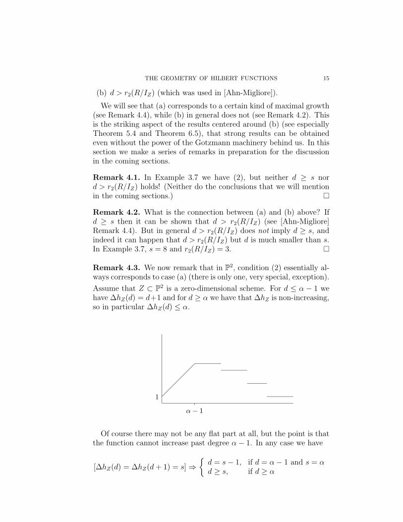
Remark 4.3. We now remark that in P2, condition (2) essentially al-

ways corresponds to case (a) (there is only one, very special, exception).

Assume that Z ⊂ P2 is a zero-dimensional scheme. For d ≤ α − 1 we

have ∆hZ(d) = d+1 and for d ≥ α we have that ∆hZ is non-increasing,so in particular ∆hZ(d) ≤ α.

��

��

�

1

α − 1

Of course there may not be any flat part at all, but the point is thatthe function cannot increase past degree α− 1. In any case we have

[∆hZ(d) = ∆hZ(d+ 1) = s] ⇒{d = s− 1, if d = α− 1 and s = αd ≥ s, if d ≥ α

16 JUAN C. MIGLIORE

In the first case in the above calculation, we have that dim(IZ)α = 1.Notice that in this case IZ is zero in degree d = α − 1, but (IZ)d+1 =

(IZ)α defines a hypersurface (or equivalently a curve) in P2.

Remark 4.4. Assume that Z ⊂ Pn is a zero-dimensional scheme. If

d ≥ s then the condition ∆hZ(d) = ∆hZ(d + 1) = s implies that thegrowth of the Artinian reduction from degree d to degree d+1 is max-imal in the sense of Definition 2.5. Indeed, the d-binomial expansionof s is

s =

(d

d

)+ · · · +

(d− s+ 1

d− s+ 1

)

so

s〈d〉 =

(d+ 1

d+ 1

)+ · · · +

(d− s+ 2

d− s+ 2

)= s

as claimed.

Remark 4.5. In practice, it usually is the case that ∆hZ having max-imal growth from degree d to degree d+1 does not imply that hZ itselfhas maximal growth from degree d to degree d+1. If it did, Gotzmann’sresults (Theorem 2.11 and Remark 2.12) would immediately apply tohZ . The interest in the results described below is that similar powerfulconclusions come from this maximal growth of the first difference (seeProposition 2.14 and Remark 2.15). And as we will see, even moresurprising is that similar results can be deduced at times even whenthe first difference does not have maximal growth.

5. General results

A by-now classical result of Davis (cf. [Davis]) is the following. Notethat there is no uniformity assumption on Z. In the next section wewill discuss the refinements that are possible when we assume UPP.

Theorem 5.1 (Davis). Let Z ⊂ P2 be a zero-dimensional scheme. If

∆hZ(d) = ∆hZ(d+ 1) = s for d ≥ s, then (IZ)d and (IZ)d+1 both havea GCD, F , of degree s. If Z is reduced then so is F . The polynomial F

defines a

{hypersurfacecurve

in P2. If Z1 ⊂ Z is the subscheme of Z lying

on F (defined by [IZ +(F )]sat) and Z2 is the “residual” scheme definedby [IZ : F ], then there are formulas relating the Hilbert functions ofIZ , IZ1 and IZ2.


Remark 5.2. It is worth mentioning that the Artinian version of The-orem 5.1 was proved earlier, by A. Iarrobino (cf. [Iarrobino2], page56).

The paper [Bigatti-Geramita-Migliore] began with the observationthat Davis’ result, Theorem 5.1, was really about maximal growth ofthe function ∆hZ(t) from degree d to degree d+ 1, thanks to Remark

4.3 and Remark 4.4 above. These remarks show that in P2, ∆hZ can

have two different kinds of maximal growth: either hZ takes on thevalue of the polynomial ring (before the initial degree of the ideal),or else ∆hZ takes the constant value s ≥ d. This latter is the onlyinteresting case.

Notice that since Z is a zero-dimensional scheme, eventually theHilbert function is constant, so eventually ∆hZ is zero. So the conditionthat ∆hZ(d) = ∆hZ(d + 1) = s directly gives us information not somuch about IZ as about (IZ)≤d, the ideal generated by the componentsof degree ≤ d. We have to deduce properties of IZ from this, viaProposition 2.14. Gotzmann’s results tell us that in a general Artinianreduction of R/IZ (which has Hilbert function ∆hZ), the degree d

component of the ideal J = (IZ ,L)(L)

agrees with the degree d component

of the saturated ideal of a subscheme of degree s in the line defined byL (cf. Remark 2.12). Since this corresponds to a hyperplane sectionby L, that means that the base locus of the linear system |Id| containsa curve of degree s, which is the GCD in question. The results aboutthe subscheme of Z lying on this GCD and the “residual” subschemecome from some algebraic arguments chasing exact sequences.

As noted in the way we phrased Davis’ theorem, this GCD can beviewed as a curve, or as a hypersurface in P

2. These correspond, re-spectively, to the interpretations (that happen to coincide in this case)that the maximal growth for ∆hZ takes the constant value s ≤ d, andit takes the largest possible growth short of being equal to the Hilbertfunction of the whole polynomial ring itself.

In [Bigatti-Geramita-Migliore] we extended this to Pn−1, and we

called these kinds of maximal growth growth like a curve, and growthlike a hypersurface, respectively. We proved many results for Z ⊂ P

n−1.In particular, we showed that viewing F in Theorem 5.1 as a curve,and viewing it as a hypersurface, both extend in separate directionswhen we move to higher projective spaces.

In this paper we focus on the former. We now give a summary of theresults in the “curve” direction found in [Bigatti-Geramita-Migliore]that do not assume UPP.

18 JUAN C. MIGLIORE

Theorem 5.3 ([Bigatti-Geramita-Migliore]). Let Z ⊂ Pn−1 be a re-

duced zero-dimensional scheme. Assume that ∆hZ(d) = ∆hZ(d+1) = sfor some d ≥ s. Then

(a) 〈(IZ)≤d〉 is the saturated ideal of a curve V of degree s. V is notnecessarily unmixed, but it is reduced and d-regular.

Let C be the unmixed one-dimensional part of V . Let Z1 be thesubscheme of Z lying on C (defined by [IZ + IC ]sat) and Z2 the residualscheme (defined by [IZ : IC ]). Then

(b) 〈(IZ1)≤d〉 = IC and IC is d-regular. (Part (a) was for V . This

one is not surprising, since V consists of C plus some points.)(c) There are formulas relating the Hilbert functions.

How might these results be improved? Recall that ∆hZ(d) =∆hZ(d + 1) = s for d ≥ s guarantees that ∆hZ has maximal growthfrom degree d to degree d+ 1.

1. Weaken the condition ∆hZ(d) = ∆hZ(d + 1) = s, e.g. to thecondition ∆hZ(d) = ∆hZ(d+1)+1 (possibly even maintaining theassumption d ≥ s). It may be that at least “usually” somethingsimilar will hold. But there will be important differences. This isstill an open direction, although in her thesis Susan Cooper (cf.[Cooper]), a student of Tony Geramita, is working on questionsrelated to this.

2. Weaken the assumption d ≥ s. This is the approach we take. Wewill assume only d > r2(R/IZ). This is a beautiful idea, conceivedby my co-author, Jeaman Ahn. It is very striking to see how muchcarries over to this case.

Theorem 5.4 ([Ahn-Migliore]). Let Z ⊂ Pn−1 be a reduced zero-

dimensional scheme. Assume that ∆hZ(d) = ∆hZ(d + 1) = s forsome d > r2(R/IZ). Then

(a) 〈(IZ)≤d〉 is the saturated ideal of a curve V of degree s. V is notnecessarily unmixed or reduced, but it is d-regular.

Let C be the unmixed one-dimensional part of V . Let Z1 be thesubscheme of Z lying on C (defined by [IZ + IC ]sat) and Z2 the residualscheme (defined by [IZ : IC ]). Then

(b) 〈(IZ1)≤d〉 = IC and C is d-regular.

(c) There are formulas relating the Hilbert functions.

(d) If we also assume that h1(ICred(d− 1)) = 0 then V is reduced

and C = Cred is d-regular.

Remark 5.5. We stress that in (a), we do not necessarily obtain thatV is reduced. This is the first new twist. If V is not reduced, then the


top dimensional part, C, is not necessarily reduced. This curve C isd-regular. If it is not reduced, however, it is supported on a reducedcurve, Cred. Surprisingly, Cred being d-regular does not follow from Cbeing d-regular, and there are examples where it is not true. But withthe extra assumption, (d) delivers this conclusion. Example 7.3 belowillustrates what can happen.

Theorem 5.4 combines different results of [Ahn-Migliore]. The proofsheavily use generic initial ideals and results of Green, Bayer, Stillman,Galligo, etc.

We end this section with a result that incorporates WLP and alsohigher differences of the Hilbert function and higher reduction number.

Theorem 5.6 ([Ahn-Migliore] Theorem 6.7). Let Z be a zero-dimen-

sional subscheme of Pn−1, n > 3, with WLP. Suppose that

∆2hZ(d) = ∆2hZ(d+ 1) = s

for r2(R/IZ) > d > r3(R/IZ). Then 〈(IZ)≤d〉 is a saturated ideal

defining a two-dimensional subscheme of degree s in Pn−1, and it is

d-regular.

6. Results on Uniform Position

We now investigate the effects of assuming that our points have UPP.We begin again in P

2.

Theorem 6.1. Let Z ⊂ P2 be a reduced set of points with UPP. Then

we have

(a) ([Geramita-Maroscia], [Maggioni-Ragusa]) The component of IZ

of least degree, α, contains an irreducible form (hence the generalsuch form is irreducible). In particular, this holds if there is onlyone such form, up to scalar multiple. This is in fact true not onlyin P

2 but also in Pn−1.

(b) ([Harris]) ∆hZ is of decreasing type, i.e.

if ∆hZ(d) > ∆hZ(d+ 1) then ∆hZ(t) > ∆hZ(t+ 1)

for all t ≥ d as long as ∆hZ(t) > 0.(c) If ∆hZ(d) = ∆hZ(d + 1) = s then s = α (see Remark 4.3),

(IZ)t = (F )t for all t ≤ d + 1, and the points of Z all lie on theirreducible curve defined by F .

As before, this theorem was also extended in [Bigatti-Geramita-

Migliore] to Pn−1 for the case of “maximal growth like a hypersurface,”

but here we focus on extending it for “maximal growth like a curve.”

20 JUAN C. MIGLIORE

(See the discussion preceding Theorem 5.3.) In the following we repeatpart of Theorem 5.3 and underline the new features.

Theorem 6.2 ([Bigatti-Geramita-Migliore]). Let Z ⊂ Pn−1 be a re-

duced zero-dimensional scheme with UPP. Assume that ∆hZ(d) =∆hZ(d+ 1) = s for some d ≥ s. Then

(a) 〈(IZ)≤d〉 is the saturated ideal of a curve V of degree s. V isreduced, d-regular, unmixed and irreducible.

(b) Since V is unmixed, its top dimensional part C is equal to V .Hence Z ⊂ C.

(c) 〈(IZ)≤d〉 = IC and IC is d-regular.

Remark 6.3. The hardest part is irreducibility, and it strongly usesthe assumption d ≥ s.

Still under the hypothesis of [Bigatti-Geramita-Migliore] that d ≥ s,the following extension of “decreasing type” was observed in [Ahn-

Migliore]. This completes the picture of extending the P2 result to

higher projective space under the assumption of “maximal growth likea curve.”

Corollary 6.4 ([Ahn-Migliore]). If Z ⊂ Pn−1 has UPP and ∆hZ(d) =

∆hZ(d+ 1) > ∆hZ(d+ 2) for some d ≥ s, then ∆hZ(t) > ∆hZ(t+ 1)for all t ≥ d+ 1 as long as ∆hZ(t) > 0.

We now turn to the situation of [Ahn-Migliore], where we only as-sume that d > r2(R/IZ). It is somewhat surprising to see what weretain and what we lose. Compare this with Theorem 5.4 (part ofwhich is repeated here).

Theorem 6.5 ([Ahn-Migliore]). Let Z ⊂ Pn−1 be a reduced zero-

dimensional scheme with UPP. Assume that ∆hZ(d) = ∆hZ(d+1) = sfor some d > r2(R/IZ). Then

(a) 〈(IZ)≤d〉 is the saturated ideal of an unmixed curve, V , of degrees, and it is d-regular. V is not necessarily reduced or irreducible.

(b) Since V is unmixed, its top dimensional part C is equal to V .Hence Z ⊂ C.

(c) 〈(IZ)≤d〉 = IC and IC is d-regular.

(d) If we also assume that h1(ICred(d− 1)) = 0 then V is reduced

and C = Cred is d-regular.

Remark 6.6. Why might we have hoped that “reduced and irredu-cible” would still hold in part (a) of Theorem 6.5? Recall the following.

• We saw in Theorem 6.1 that if Z ⊂ Pn−1 is a set of points in P

n−1

with UPP, it is known that a general element of smallest degree


α is reduced and irreducible. When this element is unique (up toscalar multiple), say F , we have 〈(IZ)≤α〉 is the saturated idealof a reduced, irreducible hypersurface which is α-regular. Thisis the base locus in degree α, and just having UPP is enough toguarantee the irreducibility.

• Recall from Theorem 6.2 that if d ≥ s then it is true that the baselocus, C, is reduced and irreducible.

In the next section we will give examples to show that in fact “re-duced and irreducible” does not necessarily hold (as opposed to merelybeing a gap in the theorem).

7. Examples

These examples will serve to illustrate that some of our results aboveare apparently close to optimal. We omit some details, and refer thereader to [Ahn-Migliore]. We will see that

1. In contrast to Corollary 6.4, for a set of points in Pn−1 with UPP

satisfying ∆hZ(d) = ∆hZ(d + 1) > ∆hZ(d + 2) for d > r2(R/IZ)(instead of d ≥ s), it is not necessarily true that ∆hZ is strictlydecreasing beyond this point. This is shown in Example 7.3.

2. In Theorem 6.5, when we assume only d > r2(R/IZ), it is in facttrue (as claimed) that V is not necessarily reduced or irreducible.This stands in contrast to Theorem 6.2, when we assumed d ≥ s.This is shown in Example 7.3.

3. Upon realizing that in Theorem 6.5 V is not necessarily reducedand irreducible, one might hope that at least the points of Z arerestricted to one component of V that is reduced and irreducible.Examples 7.4 and 7.5 show that even this is not true.

4. Examples 7.6 and 7.7 illustrate some of the difficulties of extend-ing these results past the case d > r2(R/IZ), showing that theseresults are optimal in a sense.

We begin with an example of Chardin and D’Cruz. It settles an oldquestion of independent interest.

Example 7.1 ([Chardin-D’Cruz]). Consider the family of complete in-tersectionideals

Im,n := (xmt− ymz, zn+2 − xtn+1) ⊂ k[x, y, z, t].

Then for m,n ≥ 1, reg(Im,n) = m + n + 2 while reg(√Im,n) =

mn + 2. Hence the regularity of the radical may be much larger thanthe regularity if the ideal itself!! In particular, if we take m = n = 4

22 JUAN C. MIGLIORE

then we obtain the following: I4,4 is a complete intersection of type

(5, 6). As such, it has degree 30, and has a Hilbert function whose firstdifference is

deg 0 1 2 3 4 5 6 7 8 9 10 11 12∆h 1 3 6 10 15 20 24 27 29 30 30 . . .

On the other hand,√I4,4 can be computed on a computer program,

e.g. macaulay (cf. [Bayer-Stillman]). It has degree 26 (hence I4,4 is not

reduced), and its Hilbert function has first difference

deg 0 1 2 3 4 5 6 7 8 9 10 11 12 13 14 15∆h 1 3 6 10 15 20 24 27 29 29 29 29 28 28 28 27

deg 16 17 18 19 20 21∆h 27 27 26 26 26 26 . . .

In [Chardin-D’Cruz], the authors were not so concerned with thegeometry of this curve. We will modify this slightly, taking a moregeometric approach, in Example 7.3.

Remark 7.2. Example 7.1 shows that a curve C ⊂ P3 can have the

property that reg(√IC) may be (much) larger than reg(IC). However,

it seems to still be an open question whether this can happen, forinstance, for a smooth curve. Chardin and D’Cruz also study thesurface case, where other interesting phenomena occur. For curves,see also Ravi [Ravi].

Example 7.3 ([Ahn-Migliore] Example 5.7). In this example we re-call that k has characteristic zero. We will be basing our example onthe case m = n = 4 of the example of Chardin and D’Cruz. It isobtained by taking a geometric interpretation. Let R = k[x, y, z, t].

Let Iλ = (z, t). Let F ∈ (Iλ)5 be a homogeneous polynomial that

is smooth along λ. Let I ′ = I5λ + (F ). I ′ is the saturated ideal of a

non-ACM curve of degree 5 corresponding to the divisor D := 5λ onF . In particular, viewed as a subscheme of P

3, D has degree 5.Now, choose a general element C in the linear system |6H −D| on

F . C is smooth and irreducible. Furthermore, C has degree 25 (byliaison) and Hilbert function with first difference

deg 0 1 2 3 4 5 6 7 8 9 10 11 12 13 14 15∆h 1 3 6 10 15 20 24 27 29 29 29 29 28 28 28 27

deg 16 17 18 19 20 21∆h 27 27 26 26 26 25 . . .


We now let Z consist of sufficiently many points of C, chosen gen-erally, so that IZ agrees with IC up to and including degree 21. Z hasUPP (since C is smooth), and one checks that r2(R/IZ) = r2(R/IC) =8. Taking d = 9, we see that Theorem 6.5 applies. We obtain that〈(IZ)≤9〉 is the saturated ideal of an unmixed curve V of degree 29 con-sisting of the union of C and a subcurve of D of degree 4 supported onλ, hence V is neither irreducible nor reduced. Taking d = 12, d = 15,d = 18 slices away at the non-reduced part, and taking d = 21 givesjust C.

A computation on macaulay reveals that in fact the regularity of IC

is 21. On the other hand, the curve V of degree 29 has ideal IV withregularity 9. Actually, it is worth recording the Betti diagram of IC

and IV , because they display a surprising pattern: For IV we have

total: 1 3 2

--------------------------

0: 1 - -

1: - - -

2: - - -

3: - - -

4: - 1 -

5: - 1 -

6: - - -

7: - - -

8: - 1 2

while for IC we have

total: 1 7 10 4

--------------------------------

0: 1 - - -

1: - - - -

2: - - - -

3: - - - -

4: - 1 - -

5: - 1 - -

6: - - - -

7: - - - -

8: - 1 2 -

9: - - - -

10: - - - -

11: - 1 2 1

12: - - - -

13: - - - -

14: - 1 2 1

15: - - - -

16: - - - -

17: - 1 2 1

18: - - - -

19: - - - -

24 JUAN C. MIGLIORE

20: - 1 2 1

Notice that the diagram for IV is a subdiagram of the diagram for IC ,and that there is a striking simplicity to the diagram for IC . Noticealso that V is ACM, while C is not.

Note that in the previous example, the points of Z all lie on onereduced, irreducible curve (C). It is simply the case that V containsanother component, which happens to also be non-reduced. However,now we give another example to show that it is not necessarily truethat all the points lie on one irreducible component of the base locus.

Example 7.4 ([Ahn-Migliore] Example 5.8). In Example 7.3, insteadof choosing “sufficiently many” points on C, instead choose Z to con-sist of 192 general points on C and one general point of λ. The firstdifference of the Hilbert function of Z is

deg 0 1 2 3 4 5 6 7 8 9 10 11∆hZ 1 3 6 10 15 20 24 27 29 29 29 0

Note that this is exactly the same as what we would have if wehad taken 193 general points of C. Again, r2(R/IZ) = 8. The baselocus of (IC)9 and (IC)10 is exactly the non-reduced and reducible curveof degree 29 mentioned in Example 7.3, so the Hilbert function of Zis the truncation of the Hilbert function given above. And by thegeneral choice of the points, this will continue to be true regardlessof which subsets we take. Hence Z has UPP and satisfies ∆hZ(d) =∆hZ(d + 1) = s for some d > r2(R/IZ), but not all of the pointsof Z lie on one reduced and irreducible component of the curve ofdegree s obtained by our result (since one point lies on the non-reducedcomponent).

Example 7.5. [Ahn-Migliore] Example 5.9] We produced Example 7.4by taking almost all of the points on C, and just one off of C (in fact,it was on λ). In this example we show a surprising instance where halfof the points of V are on one irreducible component and the other halfare on another irreducible component, but we still have UPP. We againomit some of the technical details.

Let Q be a smooth quadric surface in P3, and as usual by abuse of

notation we use the same letter Q to denote the quadratic form definingthis surface. Let C1 be a general curve on Q of type (1, 15), and letC2 be a general curve on Q of type (15, 1). Hence both C1 and C2 aresmooth rational curves of degree 16, and C := C1 ∪C2 is the completeintersection of Q and a form of degree 16. Note that C is arithmeticallyCohen-Macaulay, but C1 and C2 are not.


It is not difficult to compute the Hilbert functions of these curves.We record their first differences (of course there is no difference betweenbehavior of C1 and behavior of C2; this is important in the argumentgiven in [Ahn-Migliore]):

degree 0 1 2 3 4 5 6 7 8 9 10 11 12 13∆hC 1 3 5 7 9 11 13 15 17 19 21 23 25 27∆hCi 1 3 5 7 9 11 13 15 17 19 21 23 25 27

degree 14 15 16 17 18∆hC 29 31 32 32 32∆hCi 29 16 16 16 16

We now observe:

1. These first differences (hence the ideals themselves) agree throughdegree 14, and in fact the only generator before degree 15 is Q.

2. By adding these values, we see that hC(18) = 352 andhC(15) = 241.

3. Since C and Ci are curves, these values represent the Hilbertfunctions of IC + (L) and ICi

+ (L) for a general linear form L.

4. r2(R/IC) = 16 since C is an arithmetically Cohen-Macaulay curve.

Let Z1 (respectively Z2) be a general set of 176 points on C1 (re-spectively C2). So Z := Z1 ∪ Z2 is a set of 352 points whose Hilbertfunction agrees with that of C through degree 18. In particular, wehave ∆hZ(17) = ∆hZ(18) = 32 = degC. Furthermore, r2(R/IZ) = 16by our observation 4. above. Hence Theorem 6.5 applies, and we in-deed have that the component of IZ in degree 17 defines C. However,C is not irreducible. In [Ahn-Migliore] Example 5.9, it is shown that Zhas the Uniform Position Property. Thus there is no chance of show-ing that all the points must lie on a unique irreducible component inTheorem 6.5, under our hypothesis that d > r2(R/IZ) (as was done in[Bigatti-Geramita-Migliore] when d ≥ s).

To show UPP, it is enough to show that the union of any choice of t1points of Z1 (i.e. t1 general points of C1 for t1 ≤ 176) and t2 points ofZ2 (i.e. t2 general points of C2 for t2 ≤ 176) has the truncated Hilbertfunction. For example, if t1 = 150 and t2 = 160 then we have to showthat ∆H(R/IZ) has values

1 3 5 7 9 11 13 15 17 19 21 23 25 27 29 31 32 22 0.

Notice that we know that some subset has this Hilbert function, by[Geramita-Maroscia-Roberts]. We have to show that all subsets have

26 JUAN C. MIGLIORE

this Hilbert function. See [Ahn-Migliore], Example 5.9, for the details.

Example 7.6. We saw that the condition d ≥ s of [Bigatti-Geramita-Migliore] was improved in [Ahn-Migliore] to d > r2(R/IZ). There wassome loss in the strength of the result, but a surprising amount of itdid go through. One might wonder if the condition d > r2(R/IZ) canbe further improved. But in fact, we saw already in Example 3.7 andRemark 4.1 that this is not the case.

Similarly, we have the following examples:

7 general points in P3 have h-vector 1 3 3

16 general points in P3 have h-vector 1 3 6 6

30 general points in P3 have h-vector 1 3 6 10 10

etc.

In each case, r2(R/IZ) has the “expected” value, say d. We have∆hZ(d) = ∆hZ(d + 1) for d = r2(R/IZ), but clearly the base locusof (IZ)d is not one-dimensional. See Remark 2.15 as well.

Similar examples can easily be found in higher projective spaces. Adifferent sort of example can be found in Example 3.7.

Example 7.7. We return to Example 3.4 to see how the theoremsmentioned above apply to that example. Recall that we have two ideals,I1 and I2, both with h-vector (1, 3, 6, 9, 11, 11, 11). Taking s = 11, itis clear that the results from [Bigatti-Geramita-Migliore] (Theorem 5.3and Theorem 6.2) do not apply because of the hypothesis d ≥ s. Asfor the results of [Ahn-Migliore] (Theorem 5.4 and Theorem 6.5), onecan check that r2(R/I1) = 4 while r2(R/I2) = 5. Hence both resultsfrom [Ahn-Migliore] apply to I1, taking d = 5, but not to I2. Andindeed, we have seen that 〈(I1)≤5〉 is the saturated ideal of the curveC described in that example. However, it can easily be checked that〈(I2)≤5〉 is saturated, but it defines a curve of degree 10 rather than 11

(and it is not unmixed, although the unmixed part is ACM; in fact itis a complete intersection of type (2, 5).).

References

[Ahn-Migliore] J. Ahn and J. Migliore, Some Geometric Results arising from theBorel Fixed Property, preprint 2004.

[Anick] D. Anick, Thin Algebras of embedding dimension three, J. Algebra 100(1986), 235–259.

[Bayer-Stillman] D. Bayer and M. Stillman, Macaulay: A system for computationin algebraic geometry and commutative algebra. Source and object code avail-able for Unix and Macintosh computers. Contact the authors, or downloadfrom ftp://math.harvard.edu via anonymous ftp.


[Bernstein-Iarrobino] D. Bernstein and A. Iarrobino, A nonunimodal graded Goren-stein Artin algebra in codimension five, Comm. Alg. 20(8) (1992), 2323–2336.

[Bigatti-Geramita-Migliore] A. Bigatti, A.V. Geramita and J. Migliore, GeometricConsequences of Extremal Behavior in a Theorem of Macaulay, Trans. Amer.Math. Soc. 346 (1994), 203–235.

[Boij-Laksov] M. Boij and D. Laksov, Nonunimodality of Graded Gorenstein ArtinAlgebras, Proc. Amer. Math. Soc. 120 (1994), 1083–1092.

[Bolondi-Migliore] G. Bolondi and J. Migliore, Buchsbaum Liaison Classes, J. Alg.123 (1989), 426–456.

[Bruns-Herzog] W. Bruns and J. Herzog, “Cohen-Macaulay Rings, revised edi-tion,” Cambridge studies in advanced mathematics #39, Cambridge Uni-versity Press, Cambridge, 1998.

[Chardin-D’Cruz] M. Chardin and C. D’Cruz, Castelnuovo-Mumford regularity: ex-amples of curves and surfaces, J. Algebra 270 (2003), no. 1, 347–360.

[Cooper] S. Cooper, Ph.D. thesis, Queen’s University, 2005.[Davis] E.D. Davis, Complete Intersections of Codimension 2 in P

r: The Bezout-Jacobi-Segre Theorem Revisited, Rend. Sem. Mat. Univers. Politecn. Torino,43, 4 (1985), 333–353.

[Geramita-Maroscia] A.V. Geramita and P. Maroscia, The Ideal of Forms Vanish-ing at a Finite Set of Points in P

n, J. Alg. 90 (1984), 528-555.[Geramita-Maroscia-Roberts] A.V. Geramita, P. Maroscia and L. Roberts, The

Hilbert Function of a Reduced k-Algebra, J. London Math. Soc. 28 (1983),443–452.

[Geramita-Migliore] A.V. Geramita and J. Migliore, Hyperplane Sections of a

Smooth Curve in P3, Comm. Alg. 17 (1989), 3129–3164.

[Gotzmann] G. Gotzmann, Eine Bedingung fur die Flachheit und das Hilberpoly-nom eines graduierten Ringes Math. Z. 158 (1978), 61-70.

[Green1] M. Green, Restrictions of Linear Series to Hyperplanes, and some resultsof Macaulay and Gotzmann, SLN 1389, Algebraic Curves and Projective Ge-ometry, Proceedings Trento, 1988, Springer-Verlag.

[Green2] M. Green, Generic Initial Ideals, in Six lectures on Commutative Alge-bra, (Elias J., Giral J.M., Miro-Roig, R.M., Zarzuela S., eds.), Progress inMathematics 166, Birkhauser, 1998, 119–186.

[Harima-Migliore-Nagel-Watanabe] T. Harima, J. Migliore, U. Nagel and J. Watan-abe, The Weak and Strong Lefschetz Properties for Artinian k-algebras, J.Algebra 262 (2003), 99-126.

[Harris] J. Harris, The Genus of Space Curves, Math. Ann. 249 (1980), 191–204.[Harris-Eisenbud] J. Harris, D. Eisenbud, Curves in Projective Space, Sem. de

Mathematiques Superieures– Universite de Montreal (1982).[Hartshorne] R. Hartshorne, Connectedness of the Hilbert scheme, Math. Inst. des

Hautes Etudes Sci. 29 (1966), 261–304.[Hoa-Trung] L.T. Hoa and N.V. Trung. Borel-fixed ideals and reduction number, J.

Algebra 270 (2003), no. 1, 335–346.[Iarrobino1] A. Iarrobino, “Associated graded algebra of a Gorenstein Artin alge-

bra,” Memoirs Amer. Math. Soc. 107 (1994).[Iarrobino2] A. Iarrobino, “Punctual Hilbert Schemes,” Memoirs Amer. Math. Soc.

10, no. 188 (1977).

28 JUAN C. MIGLIORE

[Iarrobino-Kanev] A. Iarrobino and V. Kanev, “Power Sums, Gorenstein Algebras,and Determinantal Loci,” Springer LNM 1721 (1999).

[Kleppe] J. Kleppe, Maximal families of Gorenstein algebras, to appear in Trans.Amer. Math. Soc.

[Macaulay] F.S. Macaulay, Some properties of enumeration in the theory of modularsystems, Proc. Lond. Math. Soc. 26 (1927) 531–555.

[Maggioni-Ragusa] R. Maggioni and A. Ragusa, Connections between Hilbert Func-

tion and Geometric Properties for a Finite Set of Points in P2, Le Matem-

atiche 34, Fasc. I-II (1984), 153–170.[Migliore1] J. Migliore, “Introduction to Liaison Theory and Deficiency Modules,”

Birkhauser, Progress in Mathematics 165, 1998; 224 pp. Hardcover, ISBN0-8176-4027-4.

[MIgliore2] J. Migliore, On Linking Double Lines, Trans. Amer. Math. Soc. 294(1986), 177–185.

[Migliore-Miro-Roig1] J. Migliore and R. Miro-Roig, On the minimal free resolutionof n + 1 general forms, Trans. Amer. Math. Soc. 355 No. 1 (2003), 1–36.

[Migliore-Miro-Roig2] J. Migliore and R. Miro-Roig, Ideals of general forms and theubiquity of the Weak Lefschetz Property, J. Pure Appl. Algebra 182 (2003),79–107.

[Migliore-Miro-Roig-Nagel] J. Migliore, R. Miro-Roig and U. Nagel, Minimal Res-olution of relatively compressed level algebras, to appear in J. Algebra.

[Migliore-Nagel] J. Migliore and U. Nagel, Lifting Monomial Ideals, Comm. Algebra28 (2000) (special volume in honor of Robin Hartshorne), 5679-5701.

[Ragusa-Zappala] A. Ragusa and G. Zappala, On the reducibility of the postulationHilbert scheme, Rendiconti del Circolo Matematico di Palermo, Serie II, TomoLIII (2004), pp. 401-406

[Ravi] M.S. Ravi, Regularity of Ideals and their Radicals, manuscripta math. 68(1990), 77–87.

[Richert] B. Richert, Smallest graded Betti numbers, J. Algebra 244 (2001), 236–259.

Department of Mathematics, University of Notre Dame, Notre Dame,IN 46556, USA

E-mail address: [email protected]

the geometry of hilbert functions introductionjmiglior/hilb.pdf · the geometry of hilbert...

Documents