the geometry of schemes
TRANSCRIPT

Graduate Texts in Mathematics 197Editorial Board
S. Axler F.W. Gehring K.A. Ribet
SpringerNew YorkBerlinHeidelbergBarcelonaHong KongLondonMilanParisSingaporeTokyo

Graduate Texts in Mathematics
1 TAKEUTI/ZARING. Introduction toAxiomatic Set Theory. 2nd ed.
2 OXTOBY. Measure and Category. 2nd ed.3 SCHAEFER. Topological Vector Spaces.
2nd ed.4 HILTON/STAMMBACH. A Course in
Homological Algebra. 2nd ed.5 MAC LANE. Categories for the Working
Mathematician. 2nd ed.6 HUGHES/PIPER. Protective Planes.7 SERRE. A Course in Arithmetic.8 TAKEUTI/ZARING. Axiomatic Set Theory.9 HUMPHREYS. Introduction to Lie Algebras
and Representation Theory.10 COHEN. A Course in Simple Homotopy
Theory.11 CONWAY. Functions of One Complex
Variable I. 2nd ed.12 BEALS. Advanced Mathematical Analysis.13 ANDERSON/FULLER. Rings and Categories
of Modules. 2nd ed.14 GOLUBITSKY/GUILLEMIN. Stable Mappings
and Their Singularities.15 BERBERIAN. Lectures in Functional
Analysis and Operator Theory.16 WINTER. The Structure of Fields.17 ROSENBLATT. Random Processes. 2nd ed.18 HALMOS. Measure Theory.19 HALMOS. A Hilbert Space Problem Book.
2nd ed.20 HUSEMOLLER. Fibre Bundles. 3rd ed.21 HUMPHREYS. Linear Algebraic Groups.22 BARNES/MACK. An Algebraic Introduction
to Mathematical Logic.23 GREUB. Linear Algebra. 4th ed.24 HOLMES. Geometric Functional Analysis
and Its Applications.25 HEWITT/STROMBERG. Real and Abstract
Analysis.26 MANES. Algebraic Theories.27 KELLEY. General Topology.28 ZARISKI/SAMUEL. Commutative Algebra.
Vol.1.29 ZARISKI/SAMUEL. Commutative Algebra.
Vol.II.30 JACOBSON. Lectures in Abstract Algebra I.
Basic Concepts.31 JACOBSON. Lectures in Abstract Algebra II.
Linear Algebra.32 JACOBSON. Lectures in Abstract Algebra
III. Theory of Fields and Galois Theory.
33 HIRSCH. Differential Topology.34 SPITZER. Principles of Random Walk.
2nd ed.35 ALEXANDER/WERMER. Several Complex
Variables and Banach Algebras. 3rd ed.36 KELLEY/NAMIOKA et al. Linear
Topological Spaces.37 MONK. Mathematical Logic.38 GRAUERT/FRITZSCHE. Several Complex
Variables.39 ARVESON. An Invitation to C*-Algebras.40 KEMENY/SNELL/KNAPP. Denumerable
Markov Chains. 2nd ed.41 APOSTOL. Modular Functions and Dirichlet
Series in Number Theory.2nd ed.
42 SERRE. Linear Representations of FiniteGroups.
43 GILLMAN/JERISON. Rings of ContinuousFunctions.
44 KENDIG. Elementary Algebraic Geometry.45 LOEVE. Probability Theory I. 4th ed.46 LOEVE. Probability Theory II. 4th ed.47 MOISE. Geometric Topology in
Dimensions 2 and 3.48 SACHS/WU. General Relativity for
Mathematicians.49 GRUENBERG/WEIR. Linear Geometry.
2nd ed.50 EDWARDS. Fermat's Last Theorem.51 KLINGENBERG. A Course in Differential
Geometry.52 HARTSHORNE. Algebraic Geometry.53 MANIN. A Course in Mathematical Logic.54 GRAVER/WATKINS. Combinatorics with
Emphasis on the Theory of Graphs.55 BROWN/PEARCY. Introduction to Operator
Theory I: Elements of FunctionalAnalysis.
56 MASSEY. Algebraic Topology: AnIntroduction.
57 CROWELL/FOX. Introduction to KnotTheory.
58 KOBLITZ. p-adic Numbers, p-adicAnalysis, and Zeta-Functions. 2nd ed.
59 LANG. Cyclotomic Fields.60 ARNOLD. Mathematical Methods in
Classical Mechanics. 2nd ed.61 WHITEHEAD. Elements of Homotopy
Theory.
(continued after index)
David EisenbudJoe Harris
The Geometryof Schemes
With 40 Illustrations
Springer

David EisenbudMathematical Sciences Research
Institute1000 Centennial DriveBerkeley, CA 94720-5070USA
Joe HarrisDepartment of MathematicsHarvard UniversityCambridge, MA 02138USA
Editorial BoardS. AxlerMathematics DepartmentSan Francisco State
UniversitySan Francisco, CA 94132USA
F.W. GehringMathematics DepartmentEast HallUniversity of MichiganAnn Arbor, MI 48109USA
K.A. RibetMathematics DepartmentUniversity of California
at BerkeleyBerkeley, CA 94720-3840USA
Mathematics Subject Classification (1991): 14-02, 14A15
Library of Congress Cataloging-in-Publication DataEisenbud, David.
The geometry of schemes / David Eisenbud, Joe Harris.p. cm. — (Graduate texts in mathematics : 197)
Includes bibliographical references and index.ISBN 0-387-98637-5 (softcover : alk. paper) — ISBN 0-387-98638-3
(hardcover : alk. paper)1. Schemes (Algebraic geometry) I. Harris, Joe. II. Title.
QA564.E357 1999516.3'5—dc21 99-36219
© 2000 Springer-Verlag New York, Inc.All rights reserved. This work may not be translated or copied in whole or in part without thewritten permission of the publisher (Springer-Verlag New York, Inc., 175 Fifth Avenue, NewYork, NY 10010, USA), except for brief excerpts in connection with reviews or scholarlyanalysis. Use in connection with any form of information storage and retrieval, electronicadaptation, computer software, or by similar or dissimilar methodology now known or hereafterdeveloped is forbidden.The use of general descriptive names, trade names, trademarks, etc., in this publication, even ifthe former are not especially identified, is not to be taken as a sign that such names, asunderstood by the Trade Marks and Merchandise Marks Act, may accordingly be used freelyby anyone.
ISBN 0-387-98637-5 Springer-Verlag New York Berlin HeidelbergISBN 0-387-98638-3 Springer-Verlag New York Berlin Heidelberg
SPIN 10523686 (softcover)SPIN 10523563 (hardcover)

. . . the end of all our exploringWill be to arrive where we startedAnd know the place for the first time.
– T. S. Eliot, “Little Gidding” (Four Quartets)

Contents
I Basic Definitions 7I.1 Affine Schemes . . . . . . . . . . . . . . . . . . . . . . . . . 7
I.1.1 Schemes as Sets . . . . . . . . . . . . . . . . . . . . 9I.1.2 Schemes as Topological Spaces . . . . . . . . . . . . 10I.1.3 An Interlude on Sheaf Theory . . . . . . . . . . . . 11
References for the Theory of Sheaves . . . . . . . . 18I.1.4 Schemes as Schemes (Structure Sheaves) . . . . . . 18
I.2 Schemes in General . . . . . . . . . . . . . . . . . . . . . . 21I.2.1 Subschemes . . . . . . . . . . . . . . . . . . . . . . 23I.2.2 The Local Ring at a Point . . . . . . . . . . . . . . 26I.2.3 Morphisms . . . . . . . . . . . . . . . . . . . . . . . 28I.2.4 The Gluing Construction . . . . . . . . . . . . . . . 33
Projective Space . . . . . . . . . . . . . . . . . . . . 34I.3 Relative Schemes . . . . . . . . . . . . . . . . . . . . . . . . 35
I.3.1 Fibered Products . . . . . . . . . . . . . . . . . . . 35I.3.2 The Category of S-Schemes . . . . . . . . . . . . . 39I.3.3 Global Spec . . . . . . . . . . . . . . . . . . . . . . 40
I.4 The Functor of Points . . . . . . . . . . . . . . . . . . . . . 42
II Examples 47II.1 Reduced Schemes over Algebraically Closed Fields . . . . . 47
II.1.1 Affine Spaces . . . . . . . . . . . . . . . . . . . . . . 47II.1.2 Local Schemes . . . . . . . . . . . . . . . . . . . . . 50
II.2 Reduced Schemes over Non-Algebraically Closed Fields . . 53
Introduction 1

viii Contents
II.3 Nonreduced Schemes . . . . . . . . . . . . . . . . . . . . . 57II.3.1 Double Points . . . . . . . . . . . . . . . . . . . . . 58II.3.2 Multiple Points . . . . . . . . . . . . . . . . . . . . 62
Degree and Multiplicity . . . . . . . . . . . . . . . . 65II.3.3 Embedded Points . . . . . . . . . . . . . . . . . . . 66
Primary Decomposition . . . . . . . . . . . . . . . . 67II.3.4 Flat Families of Schemes . . . . . . . . . . . . . . . 70
Limits . . . . . . . . . . . . . . . . . . . . . . . . . . 71Examples . . . . . . . . . . . . . . . . . . . . . . . . 72Flatness . . . . . . . . . . . . . . . . . . . . . . . . 75
II.3.5 Multiple Lines . . . . . . . . . . . . . . . . . . . . . 80II.4 Arithmetic Schemes . . . . . . . . . . . . . . . . . . . . . . 81
II.4.1 Spec Z . . . . . . . . . . . . . . . . . . . . . . . . . 82II.4.2 Spec of the Ring of Integers in a Number Field . . . 82II.4.3 Affine Spaces over Spec Z . . . . . . . . . . . . . . 84II.4.4 A Conic over Spec Z . . . . . . . . . . . . . . . . . . 86II.4.5 Double Points in A1
Z . . . . . . . . . . . . . . . . . . 88
III Projective Schemes 91III.1 Attributes of Morphisms . . . . . . . . . . . . . . . . . . . 92
III.1.1 Finiteness Conditions . . . . . . . . . . . . . . . . . 92III.1.2 Properness and Separation . . . . . . . . . . . . . . 93
III.2 Proj of a Graded Ring . . . . . . . . . . . . . . . . . . . . . 95III.2.1 The Construction of ProjS . . . . . . . . . . . . . . 95III.2.2 Closed Subschemes of ProjR . . . . . . . . . . . . . 100III.2.3 Global Proj . . . . . . . . . . . . . . . . . . . . . . 101
Proj of a Sheaf of Graded OX -Algebras . . . . . . . 101The Projectivization P(E ) of a Coherent Sheaf E . 103
III.2.4 Tangent Spaces and Tangent Cones . . . . . . . . . 104Affine and Projective Tangent Spaces . . . . . . . . 104Tangent Cones . . . . . . . . . . . . . . . . . . . . . 106
III.2.5 Morphisms to Projective Space . . . . . . . . . . . . 110III.2.6 Graded Modules and Sheaves . . . . . . . . . . . . . 118III.2.7 Grassmannians . . . . . . . . . . . . . . . . . . . . . 119III.2.8 Universal Hypersurfaces . . . . . . . . . . . . . . . . 122
III.3 Invariants of Projective Schemes . . . . . . . . . . . . . . . 124III.3.1 Hilbert Functions and Hilbert Polynomials . . . . . 125III.3.2 Flatness II: Families of Projective Schemes . . . . . 125III.3.3 Free Resolutions . . . . . . . . . . . . . . . . . . . . 127III.3.4 Examples . . . . . . . . . . . . . . . . . . . . . . . . 130
Points in the Plane . . . . . . . . . . . . . . . . . . 130Examples: Double Lines in General and in P3
K . . . 136III.3.5 Bezout’s Theorem . . . . . . . . . . . . . . . . . . . 140
Multiplicity of Intersections . . . . . . . . . . . . . . 146III.3.6 Hilbert Series . . . . . . . . . . . . . . . . . . . . . 149

Contents ix
IV Classical Constructions 151IV.1 Flexes of Plane Curves . . . . . . . . . . . . . . . . . . . . 151
IV.1.1 Definitions . . . . . . . . . . . . . . . . . . . . . . . 151IV.1.2 Flexes on Singular Curves . . . . . . . . . . . . . . 155IV.1.3 Curves with Multiple Components . . . . . . . . . . 156
IV.2 Blow-ups . . . . . . . . . . . . . . . . . . . . . . . . . . . . 162IV.2.1 Definitions and Constructions . . . . . . . . . . . . 162
An Example: Blowing up the Plane . . . . . . . . . 163Definition of Blow-ups in General . . . . . . . . . . 164The Blowup as Proj . . . . . . . . . . . . . . . . . . 170Blow-ups along Regular Subschemes . . . . . . . . . 171
IV.2.2 Some Classic Blow-Ups . . . . . . . . . . . . . . . . 173IV.2.3 Blow-ups along Nonreduced Schemes . . . . . . . . 179
Blowing Up a Double Point . . . . . . . . . . . . . . 179Blowing Up Multiple Points . . . . . . . . . . . . . 181The j-Function . . . . . . . . . . . . . . . . . . . . 183
IV.2.4 Blow-ups of Arithmetic Schemes . . . . . . . . . . . 184IV.2.5 Project: Quadric and Cubic Surfaces as Blow-ups . 190
IV.3 Fano schemes . . . . . . . . . . . . . . . . . . . . . . . . . . 192IV.3.1 Definitions . . . . . . . . . . . . . . . . . . . . . . . 192IV.3.2 Lines on Quadrics . . . . . . . . . . . . . . . . . . . 194
Lines on a Smooth Quadric over an AlgebraicallyClosed Field . . . . . . . . . . . . . . . . . . . . . 194
Lines on a Quadric Cone . . . . . . . . . . . . . . . 196A Quadric Degenerating to Two Planes . . . . . . . 198More Examples . . . . . . . . . . . . . . . . . . . . 201
IV.3.3 Lines on Cubic Surfaces . . . . . . . . . . . . . . . . 201IV.4 Forms . . . . . . . . . . . . . . . . . . . . . . . . . . . . . . 204
V Local Constructions 209V.1 Images . . . . . . . . . . . . . . . . . . . . . . . . . . . . . 209
V.1.1 The Image of a Morphism of Schemes . . . . . . . . 209V.1.2 Universal Formulas . . . . . . . . . . . . . . . . . . 213V.1.3 Fitting Ideals and Fitting Images . . . . . . . . . . 219
Fitting Ideals . . . . . . . . . . . . . . . . . . . . . . 219Fitting Images . . . . . . . . . . . . . . . . . . . . . 221
V.2 Resultants . . . . . . . . . . . . . . . . . . . . . . . . . . . 222V.2.1 Definition of the Resultant . . . . . . . . . . . . . . 222V.2.2 Sylvester’s Determinant . . . . . . . . . . . . . . . . 224
V.3 Singular Schemes and Discriminants . . . . . . . . . . . . . 230V.3.1 Definitions . . . . . . . . . . . . . . . . . . . . . . . 230V.3.2 Discriminants . . . . . . . . . . . . . . . . . . . . . 232V.3.3 Examples . . . . . . . . . . . . . . . . . . . . . . . . 234

x Contents
V.4 Dual Curves . . . . . . . . . . . . . . . . . . . . . . . . . . 240V.4.1 Definitions . . . . . . . . . . . . . . . . . . . . . . . 240V.4.2 Duals of Singular Curves . . . . . . . . . . . . . . . 242V.4.3 Curves with Multiple Components . . . . . . . . . . 242
V.5 Double Point Loci . . . . . . . . . . . . . . . . . . . . . . . 246
VI Schemes and Functors 251VI.1 The Functor of Points . . . . . . . . . . . . . . . . . . . . . 252
VI.1.1 Open and Closed Subfunctors . . . . . . . . . . . . 254VI.1.2 K-Rational Points . . . . . . . . . . . . . . . . . . . 256VI.1.3 Tangent Spaces to a Functor . . . . . . . . . . . . . 256VI.1.4 Group Schemes . . . . . . . . . . . . . . . . . . . . 258
VI.2 Characterization of a Space by its Functor of Points . . . . 259VI.2.1 Characterization of Schemes among Functors . . . . 259VI.2.2 Parameter Spaces . . . . . . . . . . . . . . . . . . . 262
The Hilbert Scheme . . . . . . . . . . . . . . . . . . 262Examples of Hilbert Schemes . . . . . . . . . . . . . 264Variations on the Hilbert Scheme Construction . . . 265
VI.2.3 Tangent Spaces to Schemes in Terms of Their Func-tors of Points . . . . . . . . . . . . . . . . . . . . . . 267Tangent Spaces to Hilbert Schemes . . . . . . . . . 267Tangent Spaces to Fano Schemes . . . . . . . . . . . 271
VI.2.4 Moduli Spaces . . . . . . . . . . . . . . . . . . . . . 274
References 279
Index 285

Introduction
What schemes are
The theory of schemes is the foundation for algebraic geometry formu-lated by Alexandre Grothendieck and his many coworkers. It is the basisfor a grand unification of number theory and algebraic geometry, dreamtof by number theorists and geometers for over a century. It has strength-ened classical algebraic geometry by allowing flexible geometric argumentsabout infinitesimals and limits in a way that the classic theory could nothandle. In both these ways it has made possible astonishing solutions ofmany concrete problems. On the number-theoretic side one may cite theproof of the Weil conjectures, Grothendieck’s original goal (Deligne [1974])and the proof of the Mordell Conjecture (Faltings [1984]). In classical alge-braic geometry one has the development of the theory of moduli of curves,including the resolution of the Brill–Noether–Petri problems, by Deligne,Mumford, Griffiths, and their coworkers (see Harris and Morrison [1998]for an account), leading to new insights even in such basic areas as the the-ory of plane curves; the firm footing given to the classification of algebraicsurfaces in all characteristics (see Bombieri and Mumford [1976]); and thedevelopment of higher-dimensional classification theory by Mori and hiscoworkers (see Kollar [1987]).
No one can doubt the success and potency of the scheme-theoretic meth-ods. Unfortunately, the average mathematician, and indeed many a be-ginner in algebraic geometry, would consider our title, “The Geometry ofSchemes”, an oxymoron akin to “civil war”. The theory of schemes is widely

2 Introduction
regarded as a horribly abstract algebraic tool that hides the appeal of ge-ometry to promote an overwhelming and often unnecessary generality.
By contrast, experts know that schemes make things simpler. The ideasbehind the theory— often not told to the beginner — are directly relatedto those from the other great geometric theories, such as differential ge-ometry, algebraic topology, and complex analysis. Understood from thisperspective, the basic definitions of scheme theory appear as natural andnecessary ways of dealing with a range of ordinary geometric phenomena,and the constructions in the theory take on an intuitive geometric contentwhich makes them much easier to learn and work with.
It is the goal of this book to share this “secret” geometry of schemes.Chapters I and II, with the beginning of Chapter III, form a rapid intro-duction to basic definitions, with plenty of concrete instances worked outto give readers experience and confidence with important families of ex-amples. The reader who goes further in our book will be rewarded witha variety of specific topics that show some of the power of the scheme-theoretic approach in a geometric setting, such as blow-ups, flexes of planecurves, dual curves, resultants, discriminants, universal hypersurfaces andthe Hilbert scheme.
What’s in this book?
Here is a more detailed look at the contents:Chapter I lays out the basic definitions of schemes, sheaves, and mor-
phisms of schemes, explaining in each case why the definitions are madethe way they are. The chapter culminates with an explanation of fiberedproducts, a fundamental technical tool, and of the language of the “functorof points” associated with a scheme, which in many cases enables one tocharacterize a scheme by its geometric properties.
Chapter II explains, by example, what various kinds of schemes look like.We focus on affine schemes because virtually all of the differences betweenthe theory of schemes and the theory of abstract varieties are encounteredin the affine case— the general theory is really just the direct product of thetheory of abstract varieties a la Serre and the theory of affine schemes. Webegin with the schemes that come from varieties over an algebraically closedfield (II.1). Then we drop various hypotheses in turn and look successivelyat cases where the ground field is not algebraically closed (II.2), the schemeis not reduced (II.3), and where the scheme is “arithmetic”— not definedover a field at all (II.4).
In Chapter II we also introduce the notion of families of schemes. Familiesof varieties, parametrized by other varieties, are central and characteristicaspects of algebraic geometry. Indeed, one of the great triumphs of schemetheory— and a reason for much of its success— is that it incorporates thisaspect of algebraic geometry so effectively. The central concepts of limits,and flatness make their first appearance in section II.3 and are discussed

Introduction 3
in detail, with a number of examples. We see in particular how to takeflat limits of families of subschemes, and how nonreduced schemes occurnaturally as limits in flat families.
In all geometric theories the compact objects play a central role. In manytheories (such as differential geometry) the compact objects can be embed-ded in affine space, but this is not so in algebraic geometry. This is thereason for the importance of projective schemes, which are proper — this isthe property corresponding to compactness. Projective schemes form themost important family of nonaffine schemes, indeed the most importantfamily of schemes altogether, and we devote Chapter III to them. Aftera discussion of properness we give the construction of Proj and describein some detail the examples corresponding to projective space over the in-tegers and to double lines in three-dimensional projective space (in affinespace all double lines are equivalent, as we show in Chapter II, but this isnot so in projective space). We also discuss the important geometric con-structions of tangent spaces and tangent cones, the universal hypersurfaceand intersection multiplicities.
We devote the remainder of Chapter III to some invariants of projec-tive schemes. We define free resolutions, graded Betti numbers and Hilbertfunctions, and we study a number of examples to see what these invariantsyield in simple cases. We also return to flatness and describe its relation tothe Hilbert polynomial.
In Chapters IV and V we exhibit a number of classical constructionswhose geometry is enriched and clarified by the theory of schemes. We be-gin Chapter IV with a discussion of one of the most classical of subjects inalgebraic geometry, the flexes of a plane curve. We then turn to blow-ups, atool that recurs throughout algebraic geometry, from resolutions of singu-larities to the classification theory of varieties. We see (among other things)that this very geometric construction makes sense and is useful for such ap-parently non-geometric objects as arithmetic schemes. Next, we study theFano schemes of projective varieties—that is, the schemes parametrizingthe lines and other linear spaces contained in projective varieties— focusingin particular on the Fano schemes of lines on quadric and cubic surfaces.Finally, we introduce the reader to the forms of an algebraic variety—that is, varieties that become isomorphic to a given variety when the fieldis extended.
In Chapter V we treat various constructions that are defined locally. Forexample, Fitting ideals give one way to define the image of a morphism ofschemes. This kind of image is behind Sylvester’s classical construction ofresultants and discriminants, and we work out this connection explicitly.As an application we discuss the set of all tangent lines to a plane curve(suitably interpreted for singular curves) called the dual curve. Finally, wediscuss the double point locus of a morphism.
In Chapter VI we return to the functor of points of a scheme, and givesome of its varied applications: to group schemes, to tangent spaces, and

4 Introduction
to describing moduli schemes. We also give a taste of the way in whichgeometric definitions such as that of tangent space or of openness can beextended from schemes to certain functors. This extension represents thebeginning of the program of enlarging the category of schemes to a moreflexible one, which is akin to the idea of adding distributions to the ordinarytheory of functions.
Since we believe in learning by doing we have included a large num-ber of exercises, spread through the text. Their level of difficulty and thebackground they assume vary considerably.
Didn’t you guys already write a book on schemes?
This book represents a major revision and extension of our book Schemes:The Language of Modern Algebraic Geometry, published by Wadsworth in1992. About two-thirds of the material in this volume is new. The intro-ductory sections have been improved and extended, but the main differenceis the addition of the material in Chapters IV and V, and related materialelsewhere in the book. These additions are intended to show schemes atwork in a number of topics in classical geometry. Thus for example we defineblowups and study the blowup of the plane at various nonreduced points;and we define duals of plane curves, and study how the dual degeneratesas the curve does.
What to do with this book
Our goal in writing this manuscript has been simply to communicate to thereader our sense of what schemes are and why they have become the fun-damental objects in algebraic geometry. This has governed both our choiceof material and the way we have chosen to present it. For the first, we havechosen topics that illustrate the geometry of schemes, rather than develop-ing more refined tools for working with schemes, such as cohomology anddifferentials. For the second, we have placed more emphasis on instructiveexamples and applications, rather than trying to develop a comprehensivelogical framework for the subject.
Accordingly, this book can be used in several different ways. It could bethe basis of a second semester course in algebraic geometry, following acourse on classical algebraic geometry. Alternatively, after reading the firsttwo chapters and the first half of Chapter III of this book, the reader maywish to pass to a more technical treatment of the subject; we would recom-mend Hartshorne [1977] to our students. Thirdly, one could use this bookselectively to complement a course on algebraic geometry from a book suchas Hartshorne’s. Many topics are treated independently, as illustrations, sothat they can easily be disengaged from the rest of the text.

Introduction 5
We expect that the reader of this book will already have some famil-iarity with algebraic varieties. Good sources for this include Harris [1995],Hartshorne [1977, Chapter 1], Mumford [1976], Reid [1988], or Shafare-vich [1974, Part 1], although all these sources contain more than is strictlynecessary.
Beginners do not stay beginners forever, and those who want to applyschemes to their own areas will want to go on to a more technically orientedtreatise fairly soon. For this we recommend to our students Hartshorne’sbook Algebraic Geometry [1977]. Chapters 2 and 3 of that book containmany fundamental topics not treated here but essential to the modernuses of the theory. Another classic source, from which we both learned agreat deal, is David Mumford’s The Red Book of Varieties and Schemes[1988]. The pioneering work of Grothendieck [Grothendieck 1960; 1961a;1961b; 1963; 1964; 1965; 1966; 1967] and Dieudonne remains an importantreference.
Who helped fix it
We are grateful to many readers who pointed out errors in earlier versionsof this book. They include Leo Alonso, Joe Buhler, Herbert Clemens, Ves-selin Gashorov, Andreas Gathmann, Tom Graber, Benedict Gross, BrendanHassett, Ana Jeremias, Alex Lee, Silvio Levy, Kurt Mederer, Mircea Mus-tata, Arthur Ogus, Keith Pardue, Irena Peeva, Gregory Smith, Jason Starr,and Ravi Vakil.
Silvio Levy helped us enormously with his patience and skill. He trans-formed a crude document into the book you see before you, providing alevel of editing that could only come from a professional mathematiciandevoted to publishing.
How we learned it
Our teacher for most of the matters presented here was David Mumford.The expert will easily perceive his influence; and a few of his drawings, suchas that of the projective space over the integers, remain almost intact. It wasfrom a project originally with him that this book eventually emerged. Weare glad to express our gratitude and appreciation for what he taught us.
David EisenbudJoe Harris

IBasic Definitions
Just as topological or differentiable manifolds are made by gluing togetheropen balls from Euclidean space, schemes are made by gluing together opensets of a simple kind, called affine schemes. There is one major difference:in a manifold one point looks locally just like another, and open balls arethe only open sets necessary for the construction; they are all the sameand very simple. By contrast, schemes admit much more local variation;the smallest open sets in a scheme are so large that a lot of interesting andnontrivial geometry happens within each one. Indeed, in many schemesno two points have isomorphic open neighborhoods (other than the wholescheme). We will thus spend a large portion of our time describing affineschemes.
We will lay out basic definitions in this chapter. We have provided a seriesof easy exercises embodying and applying the definitions. The examplesgiven here are mostly of the simplest possible kind and are not necessarilytypical of interesting geometric examples. The next chapter will be devotedto examples of a more representative sort, intended to indicate the ways inwhich the notion of a scheme differs from that of a variety and to give asense of the unifying power of the scheme-theoretic point of view.
I.1 Affine Schemes
An affine scheme is an object made from a commutative ring. The rela-tionship is modeled on and generalizes the relationship between an affine
8 I. Basic Definitions
variety and its coordinate ring. In fact, one can be led to the definition ofscheme in the following way. The basic correspondence of classical algebraicgeometry is the bijection
affine varieties ←→
finitely generated, nilpotent-free ringsover an algebraically closed field K
Here the left-hand side corresponds to the geometric objects we arenaively interested in studying: the zero loci of polynomials. If we startby saying that these are the objects of interest, we arrive at the restrictedcategory of rings on the right. Scheme theory arises if we adopt the oppo-site point of view: if we do not accept the restrictions “finitely generated,”“nilpotent-free” or “K-algebra” and insist that the right-hand side includeall commutative rings, what sort of geometric object should we put on theleft? The answer is “affine schemes”; and in this section we will show howto extend the preceding correspondence to a diagram
affine varieties ←→
finitely generated, nilpotent-free ringsover an algebraically closed field K
affine schemes ←→ commutative rings with identity
We shall see that in fact the ring and the corresponding affine schemeare equivalent objects. The scheme is, however, a more natural setting formany geometric arguments; speaking in terms of schemes will also allow usto globalize our constructions in succeeding sections.
Looking ahead, the case of differentiable manifolds provides a paradigmfor our approach to the definition of schemes. A differentiable manifold Mwas originally defined to be something obtained by gluing together openballs— that is, a topological space with an atlas of coordinate charts. How-ever, specifying the manifold structure on M is equivalent to specifyingwhich of the continuous functions on any open subset of M are differen-tiable. The property of differentiability is defined locally, so the differen-tiable functions form a subsheaf C ∞(M) of the sheaf C (M) of continuousfunctions on M (the definition of sheaves is given below). Thus we maygive an alternative definition of a differentiable manifold: it is a topologicalspace M together with a subsheaf C ∞(M) ⊂ C (M) such that the pair(M, C∞(M)) is locally isomorphic to an open subset of Rn with its sheafof differentiable functions. Sheaves of functions can also be used to definemany other kinds of geometric structure— for example, real analytic man-ifolds, complex analytic manifolds, and Nash manifolds may all be definedin this way. We will adopt an analogous approach in defining schemes: a
I.1 Affine Schemes 9
scheme will be a topological space X with a sheaf O, locally isomorphic toan affine scheme as defined below.
Let R be a commutative ring. The affine scheme defined from R will becalled Spec R, the spectrum of R. As indicated, it (like any scheme) consistsof a set of points, a topology on it called the Zariski topology, and a sheafOSpecR on this topological space, called the sheaf of regular functions, orstructure sheaf of the scheme. Where there is a possibility of confusion wewill use the notation |Spec R| to refer to the underlying set or topologicalspace, without the sheaf; though if it is clear from context what we mean(“an open subset of Spec R,” for example), we may omit the vertical bars.
We will give the definition of the affine scheme Spec R in three stages,specifying first the underlying set, then the topological structure, and fi-nally the sheaf.
I.1.1 Schemes as Sets
We define a point of Spec R to be a prime — that is, a prime ideal — ofR. To avoid confusion, we will sometimes write [p] for the point of Spec Rcorresponding to the prime p of R. We will adopt the usual convention thatR itself is not a prime ideal. Of course, the zero ideal (0) is a prime if R isa domain.
If R is the coordinate ring of an ordinary affine variety V over an alge-braically closed field, Spec R will have points corresponding to the points ofthe affine variety— the maximal ideals of R — and also a point correspond-ing to each irreducible subvariety of V. The new points, corresponding tosubvarieties of positive dimension, are at first rather unsettling but turnout to be quite convenient. They play the role of the “generic points” ofclassical algebraic geometry.
Exercise I-1. Find Spec R when R is (a) Z; (b) Z/(3); (c) Z/(6);(d) Z(3); (e) C[x]; (f) C[x]/(x2).
Each element f ∈ R defines a “function”, which we also write as f , on thespace Spec R: if x = [p] ∈ Spec R, we denote by κ(x) or κ(p) the quotientfield of the integral domain R/p, called the residue field of X at x, and wedefine f(x) ∈ κ(x) to be the image of f via the canonical maps
R → R/p → κ(x).
Exercise I-2. What is the value of the “function” 15 at the point (7) ∈Spec Z? At the point (5)?
Exercise I-3. (a) Consider the ring of polynomials C[x], and let p(x) bea polynomial. Show that if α ∈ C is a number, then (x−α) is a primeof C[x], and there is a natural identification of κ((x−α)) with C suchthat the value of p(x) at the point (x − α) ∈ Spec C[x] is the numberp(α).

10 I. Basic Definitions
(b) More generally, if R is the coordinate ring of an affine variety V over analgebraically closed field K and p is the maximal ideal correspondingto a point x ∈ V in the usual sense, then κ(x) = K and f(x) is thevalue of f at x in the usual sense.
In general, the “function” f has values in fields that vary from pointto point. Moreover, f is not necessarily determined by the values of this“function”. For example, if K is a field, the ring R = K[x]/(x2) has onlyone prime ideal, which is (x); and thus the element x ∈ R, albeit nonzero,induces a “function” whose value is 0 at every point of Spec R.
We define a regular function on Spec R to be simply an element of R.So a regular function gives rise to a “function” on SpecR, but is not itselfdetermined by the values of this “function”.
I.1.2 Schemes as Topological Spaces
By using regular functions, we make Spec R into a topological space; thetopology is called the Zariski topology. The closed sets are defined as follows.For each subset S ⊂ R, let
V (S) = x ∈ Spec R | f(x) = 0 for all f ∈ S = [p] ∈ Spec R | p ⊃ S.The impulse behind this definition is to make each f ∈ R behave as
much like a continuous function as possible. Of course the fields κ(x) haveno topology, and since they vary with x the usual notion of continuitymakes no sense. But at least they all contain an element called zero, soone can speak of the locus of points in Spec R on which f is zero; and iff is to be like a continuous function, this locus should be closed. Sinceintersections of closed sets must be closed, we are led immediately to thedefinition above: V (S) is just the intersection of the loci where the elementsof S vanish.
For the family of sets V (S) to be the closed sets of a topology it isnecessary that it be closed under arbitrary intersections; from the descrip-tion above it is clear that for any family of sets Sa we have
⋂a V (Sa) =
V(⋃
a Sa
), as required. It is worth noting also that, if I is the ideal gener-
ated by S, then V (I) = V (S).An open set in the Zariski topology is simply the complement of one of
the sets V (S). The open sets corresponding to sets S with just one elementwill play a special role, essentially because they are again spectra of rings;for this reason they get a special name and notation. If f ∈ R, we definethe distinguished (or basic) open subset of X = Spec R associated with fto be
Xf = |Spec R| \ V (f).
The points of Xf — that is, the prime ideals of R that do not contain f —are in one-to-one correspondence with the prime ideals of the localization

I.1 Affine Schemes 11
Rf of R obtained by adjoining an inverse to f , via the correspondence thatsends p ⊂ R to pRf ⊂ Rf . We may thus identify Xf with the points ofSpec Rf , an indentification we will make implicitly throughout the remain-der of this book.
The distinguished open sets form a base for the Zariski topology in thesense that any open set is a union of distinguished ones:
U = Spec R \ V (S) = Spec R \⋂f∈S
V (f) =⋃f∈S
(Spec R)f .
Distinguished open sets are also closed under finite intersections; since aprime ideal contains a product if and only if it contains one of the factors,we have ⋂
i=1,...,n
(Spec R)fi = (Spec R)g,
where g is the product f1 · · · fn. In particular, any distinguished open setthat is a subset of the distinguished open set (Spec R)f has the form(Spec R)fg for suitable g.
Spec R is almost never a Hausdorff space— the open sets are simply toolarge. In fact, the only points of SpecR that are closed are those corre-sponding to maximal ideals of R. In general, it is clear that the smallestclosed set containing a given point [p] must be V (p), so the closure of thepoint [p] consists of all [q] such that q ⊃ p. The point [p] is closed if and onlyif p is maximal. Thus in the case where R is the affine ring of an algebraicvariety V over an algebraically closed field, the points of V correspond pre-cisely to the closed points of Spec R, and the closed points contained inthe closure of the point [p] are exactly the points of V in the subvarietydetermined by p.
Exercise I-4. (a) The points of Spec C[x] are the primes (x−a), for everya ∈ C, and the prime (0). Describe the topology. Which points areclosed? Are any of them open?
(b) Let K be a field and let R be the local ring K[x](x). Describe thetopological space Spec R. (The answer is given later in this section.)
To complete the definition of Spec R, we have to describe the structuresheaf, or sheaf of regular functions on X. Before doing this, we will takea moment out to give some of the basic definitions of sheaf theory and toprove a proposition that will be essential later on (Proposition I-12).
I.1.3 An Interlude on Sheaf Theory
Let X be any topological space. A presheaf F on X assigns to each openset U in X a set, denoted F (U), and to every pair of nested open setsU ⊂ V ⊂ X a restriction map
resV,U : F (V ) → F (U)

12 I. Basic Definitions
satisfying the basic properties that
resU,U = identity
andresV,U resW,V = resW,U for all U ⊂ V ⊂ W ⊂ X.
The elements of F (U) are called the sections of F over U ; elements ofF (X) are called global sections.
Another way to express this is to define a presheaf to be a contravariantfunctor from the category of open sets in X (with a morphism U → Vfor each containment U ⊆ V ) to the category of sets. Changing the targetcategory to abelian groups, say, we have the definition of a presheaf ofabelian groups, and the same goes for rings, algebras, and so on.
One of the most important constructions of this type is that of a presheafof modules F over a presheaf of rings O on a space X. Such a thing is apair consisting of
for each open set U of X, a ring O(U) and an O(U)-module F (U)
and
for each containment U ⊇ V, a ring homomorphism α : O(U) →O(V ) and a map of sets F (U) → F (V ) that is a map of O(U)-modules if we regard F (V ) as an O(U)-module by means of α.
A presheaf (of sets, abelian groups, rings, modules, and so on) is calleda sheaf if it satisfies one further condition, called the sheaf axiom. Thiscondition is that, for each open covering U =
⋃a∈A Ua of an open set
U ⊂ X and each collection of elements
fa ∈ F (Ua) for each a ∈ A
having the property that for all a, b ∈ A the restrictions of fa and fb toUa ∩ Ub are equal, there is a unique element f ∈ F (U) whose restrictionto Ua is fa for all a.
A trivial but occasionally confusing point deserves a remark. The emptyset ∅ is of course an open subset of Spec R, and can be written as the unionof an empty family (that is, the indexing set A in the preceding paragraphis empty). Therefore the sheaf axiom imply that any sheaf has exactly onesection over the empty set. In particular, for a sheaf F of rings, F (∅) isthe zero ring (where 0 = 1). Note that the zero ring has no prime ideals atall— it is the only ring with unit having this property, if one accepts theaxiom of choice— so that its spectrum is ∅.
Exercise I-5. (a) Let X be the two-element set 0, 1, and make X intoa topological space by taking each of the four subsets to be open. Asheaf on X is thus a collection of four sets with certain maps betweenthem; describe the relations among these objects. (X is actually Spec Rfor some rings R; can you find one?)

I.1 Affine Schemes 13
(b) Do the same in the case where the topology of X = 0, 1 has asopen sets only ∅, 0 and 0, 1. Again, this space may be realized asSpec R.
If F is a presheaf on X and U is an open subset of X, we may define apresheaf F |U on U, called the restriction of F to U, by setting F |U (V ) =F (V ) for any open subset V of U, the restriction maps being the same asthose of F as well. It is easy to see that, if F is actually a sheaf, so is F |U .
In the sequel we shall work exclusively with presheaves and sheaves ofthings that are at least abelian groups, so we will usually omit the phrase“of abelian groups”. Given two presheaves of abelian groups, one can definetheir direct sum, tensor product, and so on, open set by open set; thus, forexample, if F and G are presheaves of abelian groups, we define F ⊕G by
(F ⊕ G )(U) := F (U) ⊕ G (U) for any open set U.
This always produces a presheaf, and if F and G are sheaves then F ⊕ Gwill be one as well. Tensor product is not as well behaved: even if F andG are sheaves, the presheaf defined by
(F ⊗ G )(U) := F (U) ⊗ G (U)
may not be, and we define the sheaf F ⊗ G to be the sheafification of thispresheaf, as described below.
The simplest sheaves on any topological space X are the sheaves of lo-cally constant functions with values in a set K — that is, sheaves K whereK (U) is the set of locally constant functions from U to K; if K is a group,we may make K into a sheaf of groups by pointwise addition. Similarly,if K is a ring and we define multiplication in K (U) to be pointwise mul-tiplication, then K becomes a sheaf of rings. When K has a topology, wecan define the sheaf of continuous functions with values in K as the sheafC, where C (U) is the set of continuous functions from U to K, again withpointwise addition. If X is a differentiable manifold, there are also sheavesof differentiable functions, vector fields, differential forms, and so on.
Generally, if π : Y → X is any map of topological spaces, we may definethe sheaf I of sections of π; that is, for every open set U of X we defineI (U) to be the set of continuous maps σ : U → π−1U such that π σ = 1,the identity on U (such a map being a section of π in the set-theoreticalsense: elements of F (U) for any sheaf F are called sections by extensionfrom this case).
Exercise I-6. (For readers familiar with vector bundles.) Let V be a vec-tor bundle on a topological space X. Check that the sheaf of sections of V isa sheaf of modules over the sheaf of continuous functions on X. (Sheaves ofmodules in general may in this way be seen as generalized vector bundles.)
Another way to describe a sheaf is by its stalks. For any presheaf F andany point x ∈ X, we define the stalk Fx of F at x to be the direct limit

14 I. Basic Definitions
of the groups F (U) over all open neighborhoods U of x in X — that is, bydefinition,
Fx = lim−→x∈UF (U)
=
⎧⎪⎪⎪⎪⎨⎪⎪⎪⎪⎩
the disjoint union of F (U) over all open sets U containing x,modulo the equivalence relation σ ∼ τ if σ ∈ F (U), τ ∈ F (V ),and there is an open neighborhood W of x contained in U ∩ Vsuch that the restrictions of σ and τ to W are equal:
resU,W σ = resV,W τ .
⎫⎪⎪⎪⎪⎬⎪⎪⎪⎪⎭
For every x ∈ U there is a map F (U) → Fx, sending a section s to theequivalence class of (U, s); this class is denoted sx. If F is a sheaf, a sections ∈ F (U) of F over U is determined by its images in the stalks Fx for allx ∈ U — equivalently, s = 0 if and only if sx = 0 for all x ∈ U. This followsfrom the sheaf axiom: to say that sx = 0 for all x ∈ U is to say that foreach x there is a neighborhood Ux of x in U such that resU,Ux
(s) = 0, andthen it follows that s = 0 in F (U).
This notion of stalks has a familiar geometric content: it is an abstractionof the notion of rings of germs. For example, if X is an analytic manifoldof dimension n and Oan
X is the sheaf of analytic functions on X, the stalkof Oan
X at x is the ring of germs of analytic functions at x— that is, thering of convergent power series in n variables.
Exercise I-7. Find the stalks of the sheaves you produced for Exercises I-5and I-6.
Exercise I-8. Topologize the disjoint union F =⋃
Fx by taking as abase for the open sets of F all sets of the form
V (U, s) := (x, sx) : x ∈ U,where U is an open set and s is a fixed section over U .
(a) Show that the natural map π : F → X is continuous, and that, forU and s ∈ F (U), the map σ : x → sx from U to F is a continuoussection of π over U (that is, it is continuous and π σ is the identityon U).
(b) Conversely, show that any continuous map σ : U → F such that π σis the identity on U arises in this way.Hint. Take x ∈ U and a basic open set V (V, t) containing σ(x), whereV ⊂ U . What relation does t have to σ?
This construction shows that the sheaf of germs of sections of π : F → Xis isomorphic to F , so any sheaf “is” the sheaf of germs of sections of asuitable map. In early works sheaves were defined this way. The topologicalspace F is called the “espace etale” of the sheaf, because its open sets are“stretched out flat” over open sets of X .

I.1 Affine Schemes 15
A morphism ϕ : F → G of sheaves on a space X is defined simply tobe a collection of maps ϕ(U) : F (U) → G (U) such that for every inclusionU ⊂ V the diagram
F (V )ϕ(V ) G (V )
F (U)
resV,U
ϕ(U) G (U)
resV,U
commutes. (In categorical language, a morphism of sheaves is just a naturaltransformation of the corresponding functors from the category of open setson X to the category of sets.)
A morphism ϕ : F → G induces as well a map of stalks ϕx : Fx → Gx
for each x ∈ X . By the sheaf axiom, the morphism is determined by theinduced maps of stalks: if ϕ and ψ are morphisms such that ϕx = ψx forall x ∈ X, then ϕ = ψ.
We say that a map ϕ : F → G of sheaves is injective, surjective, orbijective if each of the induced maps ϕx : Fx → Gx on stalks has thecorresponding property. The following exercises show how these notionsare related to their more naive counterparts defined in terms of sections onarbitrary sets.
Exercise I-9. Show that, if ϕ : F → G is a morphism of sheaves, thenϕ(U) is injective (respectively, bijective) for all open sets U ⊂ X if andonly if ϕx is injective (respectively, bijective) for all points x ∈ X.
Exercise I-10. Show that Exercise I-9 is false if the condition “injective”is replaced by “surjective” by checking that in each of the following exam-ples the maps induced by ϕ on stalks are surjective, but for some open setU the map ϕ(U) : F (U) → G (U) is not surjective.
(a) Let X be the topological space C \ 0, let F = G be the sheaf ofnowhere-zero, continuous, complex-valued functions, and let ϕ be themap sending a function f to f 2.
(b) Let X be the Riemann sphere CP1 = C∪∞ and let G be the sheaf ofanalytic functions. Let F1 be the sheaf of analytic functions vanishingat 0; that is, F1(U) is the set of analytic functions on U that vanishat 0 if 0 ∈ U, and the set of all analytic functions on U if 0 /∈ U.Similarly, let F2 be the sheaf of analytic functions vanishing at ∞. LetF = F1 ⊕ F2, and let ϕ : F → G be the addition map.
(c) Find an example of this phenomenon in which the set X consists ofthree points.
These examples are the beginning of the cohomology theory of sheaves;the reader will find more in this direction in the references on sheaves listedon page 18.

16 I. Basic Definitions
If F is a presheaf on X, we define the sheafification of F to be theunique sheaf F ′ and morphism of presheaves ϕ : F → F ′ such that forall x ∈ X the map ϕx : Fx → F ′
x is an isomorphism. More explicitly, thesheaf F ′ may be defined by saying that a section of F ′ over an open setU is a map σ that takes each point x ∈ U to an element in Fx in such away that σ is locally induced by sections of F ; by this we mean that thereexists an open cover of U by open sets Ui and elements si ∈ F (Ui) suchthat σ(x) = (si)x for x ∈ Ui. The map F → F ′ is defined by associatingto s ∈ F (U) the function x → sx ∈ Fx. The sheaf F ′ should be thoughtof as the sheaf “best approximating” the presheaf F.
Exercise I-11. Here is an alternate construction for F ′: topologize thedisjoint union F =
⋃Fx exactly as in Exercise I-8; then let F ′ be the
sheaf of sections of the natural map π : F → X . Convince yourself thatthe two constructions are equivalent, and that the result does have theuniversal property stated at the beginning of the preceding paragraph.
If ϕ : F → G is an injective map of sheaves, we will say that F is asubsheaf of G. We often write F ⊂ G , omitting ϕ from the notation. If ϕ :F → G is any map of sheaves, the presheaf Kerϕ defined by (Kerϕ)(U) =Ker(ϕ(U)) is a subsheaf of F .
The notion of a quotient is more subtle. Suppose F and G are presheavesof abelian groups, where F injects in G . The quotient of G by F aspresheaves is the presheaf H defined by H (U) = G (U)/F (U). But ifF and G are sheaves, H will generally not be a sheaf, and we must definetheir quotient as sheaves to be the sheafification of H , that is, G /F := H ′.The natural map from H to its sheafification H ′, together with the mapof presheaves G → H , defines the quotient map from G to G /F. Thismap is the cokernel of ϕ.
The significance of the sheaf axiom is that sheaves are defined by localproperties. We give two aspects of this principle explicitly.
In our applications to schemes, we will encounter a situation where weare given a base B for the open sets of a topological space X, and wewill want to specify a sheaf F just by saying what the groups F (U) andhomomorphisms resV,U are for open sets U of our base and inclusions U ⊂V of basic sets. The next proposition is exactly the tool that says we cando this.
We say that a collection of groups F (U) for open sets U ∈ B and mapsresV,U : F (V ) → F (U) for V ⊂ U form a B-sheaf if they satisfy thesheaf axiom with respect to inclusions of basic open sets in basic open setsand coverings of basic open sets by basic open sets. (The condition in thedefinition that sections of Ua, Ub ∈ B agree on Ua ∩ Ub must be replacedby the condition that they agree on any basic open set V ∈ B such thatV ⊂ Ua ∩ Ub.)
Proposition I-12. Let B be a base of open sets for X.

I.1 Affine Schemes 17
(i) Every B-sheaf on X extends uniquely to a sheaf on X.
(ii) Given sheaves F and G on X and a collection of maps
ϕ(U) : F (U) → G (U) for all U ∈ B
commuting with restrictions, there is a unique morphism ϕ : F → Gof sheaves such that ϕ(U) = ϕ(U) for all U ∈ B.
Beginning of the proof. For any open set U ⊂ X, define F (U) as the in-verse limit of the sets F (V ), where V runs over basic open sets containedin U :
F (U) = lim←−V ⊂U, V ∈BF (V )
=
the set of families (fV )V ⊂U, V ∈B ∈∏V ⊂U, V ∈B F (V ) such
that resV,W (fV )=fW whenever W ⊂V ⊂U with V, W ∈B.
The restriction maps are defined immediately from the universal propertyof the inverse limit.
Exercise I-13. Complete the proof of the proposition by checking thesheaf axioms and showing that, for U ∈ B, the new definition of F agreeswith the old one.
The second application, which is really a special case of the first, saysthat to define a sheaf it is enough to give it on each open set of an opencover, as long as the definitions are compatible.
Corollary I-14. Let U be an open covering of a topological space X. IfFU is a sheaf on U for each U ∈ U , and if
ϕUV : FU |U∩V → FV |U∩V
are isomorphisms satisfying the compatibility conditions
ϕV W ϕUV = ϕUW on U ∩ V ∩ W,
for all U, V, W ∈ U , there is a unique sheaf F on X whose restrictionto each U ∈ U is isomorphic to FU via isomorphisms ΨU : F |U → FU
compatible with the isomorphisms ϕUV —in other words, such that
ϕUV ΨU |U∩V = ΨV |U∩V : F |U∩V → FV |U∩V
for all U and V in U .
Proof. The open sets contained in some U ∈ U form a base B for thetopology of X. For each such set V we choose arbitrarily a set U thatcontains it, and define F (V ) = FU (V ). If for some W ⊂ V the value F (W )has been defined with reference to a different FU ′ , we use the isomorphismϕUU ′ to define the restriction maps. These maps compose correctly becauseof the compatibility conditions on the isomorphisms ϕUU ′ . Thus we have aB-sheaf, and therefore a sheaf.

18 I. Basic Definitions
The pushforward operation on sheaves is so basic (and trivial) that weintroduce it here: If α : X → Y is a continuous map on topological spacesand F is a presheaf on X, we define the pushforward α∗F of F by α tobe the presheaf on Y given by
α∗F (V ) := F (α−1(V )) for any open V ⊂ Y.
Of course, the pushforward of a sheaf of abelian groups (rings, modulesover a sheaf of rings, and so on) is again of the same type.
Exercise I-15. Show that the pushforward of a sheaf is again a sheaf.
References for the Theory of Sheaves. Serre’s landmark paper [1955],which established sheaves as an important tool in algebraic geometry, is stilla wonderful source of information. Godement [1964] and Swan [1964] aremore systematic introductions. Hartshorne [1977, Chapter II] contains anexcellent account adapted to the technical requirements of scheme theory;it is a simplified version of that found in Grothendieck [1961a; 1961b; 1963;1964; 1965; 1966; 1967]. Some good references for the analytic case areForster [1981] (especially for an introduction to cohomology) and Gunning[1990].
I.1.4 Schemes as Schemes (Structure Sheaves)
We return at last to the definition of the scheme X = Spec R. We will com-plete the construction by specifying the structure sheaf OX = OSpec R. Asindicated above, we want the relationship between SpecR and R to gener-alize that between an affine variety and its coordinate ring; in particular,we want the ring of global sections of the structure sheaf OX to be R.
We thus wish to extend the ring R of functions on X to a whole sheafof rings. This means that for each open set U of X, we wish to give a ringOX(U); and for every pair of open sets U ⊂ V we wish to give a restrictionhomomorphism
resV,U : OX(V ) → OX(U)
satisfying the various axioms above. It is quite easy to say what the ringsOX(U) and the maps resV,U should be for distinguished open sets U andV : we set
OX(Xf ) = Rf .
If Xf ⊃ Xg, some power of g is a multiple of f (recall that the radicalof (f) is the intersection of the primes containing f). Thus the restrictionmap resXf ,Xg
can be defined as the localization map Rf → Rfg = Rg. ByProposition I-12, this will suffice to define the structure sheaf O, as longas we verify that it satisfies the sheaf axiom with respect to coverings ofdistinguished opens by distinguished opens. Before doing this, in Proposi-tion I-18 below, we exhibit a simple but fundamental lemma that describesthe coverings of affine schemes by distinguished open sets.

I.1 Affine Schemes 19
Lemma I-16. Let X = Spec R, and let fa be a collection of elements ofR. The open sets Xfa cover X if and only if the elements fa generate theunit ideal. In particular, X is quasicompact as a topological space.
Recall that quasicompact means that every open cover has a finite sub-cover; the quasi is there because the space is not necessarily Hausdorff. Infact, schemes are almost never Hausdorff! Unfortunately, this fact vitiatesmost of the usual advantages of compactness. For example, in contrast tothe situation for compact manifolds, say, the continuous image of one affinescheme in another need not be closed. For this reason, we will discuss inSection III.1 a better “compactness” notion, called properness, which willplay just as important a role as compactness does in the usual geometrictheories.
Proof. The Xfa cover X if and only if no prime of R contains all the fa,which happens if and only if the fa generate the unit ideal; this proves thefirst statement. To prove the second, note first that every open cover hasa refinement of the form X =
⋃Xfa , where each fa ∈ R. Since the Xfa
cover X , the fa generate the unit ideal, so the element 1 can be writtenas a linear combination— necessarily finite— of the fa. Taking just the fa
involved in this expansion of 1, we see that the cover X =⋃
Xfa , and withit the original cover, has a finite subcover.
Exercise I-17. If R is Noetherian, every subset of Spec R is quasicompact.
Proposition I-18. Let X = Spec R, and suppose that Xf is covered byopen sets Xfa ⊂ Xf .
(a) If g, h ∈ Rf become equal in each Rfa , they are equal.
(b) If for each a there is ga ∈ Rfa such that for each pair a and b the imagesof ga and gb in Rfafb
are equal, then there is an element g ∈ Rf whoseimage in Rfa is ga for all a.
Equivalently, if B is the collection of distinguished open sets Spec Rf
of Spec R, and if we set OX(Spec Rf ) := Rf , then OX is a B-sheaf. ByProposition I-12, OX extends uniquely to a sheaf on X.
Definition I-19. The sheaf OX defined in the proposition is called thestructure sheaf of X or the sheaf of regular functions on X.
Proof of Proposition I-18. We begin with the case f = 1, so Rf = R andXf = X.
For the first part, observe that if g and h become equal in each Xfa theng − h is annihilated by a power of each fa. Since by Lemma I-16 we mayassume that the cover is finite, this implies that g − h is annihilated bya power of the ideal generated by all the fN
a for some N. But this idealcontains a power of the ideal generated by all the fa, which is the unitideal. Thus g = h in R.

20 I. Basic Definitions
For part (b), we will use an argument analogous to the classical partitionof unity to piece together the elements ga into a single element g ∈ R. Forlarge N the product fN
a ga ∈ Rfa is the image of an element ha ∈ R. ByLemma I-16 we may assume the covering Xfa is finite, and it follows thatone N will do for all a. Next, since ga and gb become equal in Xfafb
, wemust have
fNb ha = (fafb)Nga = (fafb)Ngb = fN
a hb
for large N . Again, since we have assumed the covering Xfa is finite, oneN will do for all a and b. By Lemma I-16 the elements fa ∈ R generate theunit ideal, and hence so do the elements fN
a , and we may write
1 =∑
a
eafNa
for some collection ea ∈ R; this is our partition of unity. We claim that
g =∑
a
eaha
is the element of R we seek. Indeed, for each b, we have in Rfb
fNb g =
∑a
fNb eaha =
∑a
fNa eahb = hb = fN
b gb,
so g becomes equal to gb on Xfb, as required.
Returning to the case of arbitrary f , set X ′ = Xf , R′ = Rf , f ′a = ffa;
then X ′ = Spec R′ and X ′f ′
a= Xfa , so we can apply the case already proved
to the primed data.
The proposition is still valid, and has essentially the same proof, if wereplace Rf and Rfa by Mf and Mfa for any R-module M.
Exercise I-20. Describe the points and the sheaf of functions of each ofthe following schemes.
(a) X1 = Spec C[x]/(x2). (b) X2 = Spec C[x]/(x2 − x).
(c) X3 = Spec C[x]/(x3 − x2). (d) X4 = Spec R[x]/(x2 + 1) .
In contrast with the situation in many geometric theories (though similarto the situation in the category of complex manifolds), there may be reallyrather few regular functions on a scheme. For example, when we definearbitrary schemes, we shall see that the schemes that are the analoguesof compact manifolds may have no nonconstant regular functions on themat all. For this reason, partially defined functions on a scheme X —thatis, elements OX(U) for some open dense subset U — play an unusuallylarge role. They are called rational functions on X because in the caseX = Spec R with R a domain, and U = Xf , the elements of OX(Xf ) = Rf
are ratios of elements in R. In the cases of most interest, we shall see thatevery nonempty open set is dense in X, so the behavior of rational functionsreflects the properties of X as a whole.

I.2 Schemes in General 21
Exercise I-21. Let U be the set of open and dense sets in X . Computethe ring of rational functions
lim−→U∈UOX(U) :=⎧⎨
⎩the disjoint union of OX(U) for all U ∈ U , modulo the equiva-lence relation σ ∼ τ if σ ∈ OX(U), τ ∈ OX(V ), and the restric-tions of σ and τ are equal on some W ∈U contained in U ∩ V
⎫⎬⎭ ,
first in the case where R is a domain and then for an arbitrary Noetherianring.
Example I-22. Another very simple example will perhaps help to fixthese ideas. Let K be a field, and let R = K[x](x), the localization of thepolynomial ring in one variable X at the maximal ideal (x). The schemeX = Spec R has only two points, the two prime ideals (0) and (x) of R. Asa topological space, it has precisely three open sets,
∅ ⊂ U := (0) ⊂ (0), (x) = X.
U and ∅ are distinguished open sets, since (0) = Xx. The sheaf OX isthus easy to describe. It has values OX(X) = R = K[x](x) and OX(U) =K(x), the field of rational functions. The restriction map from the first tothe second is the natural inclusion.
Exercise I-23. Give a similarly complete description for the structuresheaf of the scheme Spec K[x]. (The answer is given in Chapter II.)
I.2 Schemes in General
After this lengthy description of affine schemes, it is easy to define schemesin general. A scheme X is simply a topological space, called the support ofX and denoted |X | or supp X, together with a sheaf OX of rings on X , suchthat the pair (|X |, OX) is locally affine. Locally affine means that |X | iscovered by open sets Ui such that there exist rings Ri, and homeomorphismsUi
∼= |Spec Ri| with OX |Ui∼= OSpec Ri .
To better understand this definition, we must identify the key propertiesof the structure sheaf of an affine scheme. Let X be any topological spaceand let O be a sheaf of rings on it. We call the pair (X, O) a ringed space,and ask when it is isomorphic to an affine scheme (|Spec R|, OSpecR). Notethat if (X, O) were an affine scheme then it would have to be the schemeSpec R.
Now let (X, O) be any ringed space, and let R = O(X). For any f ∈ Rwe can define a set Uf ⊂ X as the set of points x ∈ X such that f mapsto a unit of the stalk Ox. If (X, O) is an affine scheme we must have:
(i) O(Uf ) = R[f−1].

22 I. Basic Definitions
However, this condition is not enough; it does not even force the existenceof a map between X and |Spec R|. To give such a map, we need to assumea further condition on O that is posessed by affine schemes:
(ii) The stalks Ox of O are local rings.
A ringed space (X, O) satisfying (ii) is often called a local ringed space.If (X, O) satisfies (ii), there is a natural map X → |Spec O(X)| that takes
x ∈ X to the prime ideal of O(X) that is the preimage of the maximal idealof Ox. The third condition for (X, O) to be an affine scheme is this:
(iii) The map X → |Spec O(X)| is a homeomorphism.
Given these considerations, we say that a pair (X, O) is affine if it satisfies(i)–(iii). The definition of scheme given above now becomes: A pair (X, O)is a scheme if it is locally affine.
Again, where there is no danger of confusion, we will use the same letterX to denote the scheme and the underlying space |X |, as in the construction“let p ∈ X be a point.”
Exercise I-24. (a) Take Z = Spec C[x], let X be the result of identifyingthe two closed points (x) and (x− 1) of |Z|, and let ϕ : Z → X be thenatural projection. Let O be ϕ∗OZ , a sheaf of rings on X . Show that(X, O) satisfies condition (i) above for all elements f ∈ O(X) = C[x],but does not satisfy condition (ii). Note that there is no natural mapX → |Spec C[x]|.
(b) Take Z = Spec C[x, y], the scheme corresponding to the affine plane,and let X be the open subset obtained by leaving out the origin inthe plane, that is, X = |Z| − (x, y). Let O be the sheaf OZ |X (thatis, O(V ) = OZ(V ) for any open subset V ⊂ X ⊂ |Z|.) Show thatO(X) = C[x, y], that X, O satisfies condition (i) and (ii), and that thenatural map X → |Spec O(X)| is the inclusion X ⊂ |Z|.
Some notation and terminology are in order at this point.A regular function on an open set U ⊂ X is a section of OX over U . A
global regular function is a regular function on X .The stalks OX,x of the structure sheaf OX at the points x ∈ X are called
the local rings of OX . The residue field of OX,x is denoted by κ(x). Justas in the situation of Section I.1.1, a section of OX can be thought of as a“function” taking values in these fields κ(x): if f ∈ OX(U) and x ∈ U , theimage of f under the composite
OX(U) → OX,x → κ(x)
is the value of f at x.
Exercise I-25 (the smallest nonaffine scheme). Let X be the topologicalspace with three points p, q1, and q2. Topologize X by making X1 := p, q1

I.2 Schemes in General 23
and X2 := p, q2 open sets (so that, in addition, ∅, p, and X itself areopen). Define a presheaf O of rings on X by setting
O(X) = O(X1) = O(X2) = K[x](x), O(p) = K(x),
with restriction maps O(X) → O(Xi) the identity and O(Xi) → O(p)the obvious inclusion. Check that this presheaf is a sheaf and that (X, O) isa scheme. Show that it is not an affine scheme. (Geometrically, the scheme(X, O) is the “germ of the doubled point” in the scheme called X1 inExercise I-44.)
I.2.1 Subschemes
Let U be an open subset of a scheme X. The pair (U, OX |U ) is againa scheme, though this is not completely obvious. To check it, note thatat least a distinguished open set of an affine scheme is again an affinescheme: if X = Spec R and U = Xf , then (U, OX |U ) = Spec Rf . Since thedistinguished open sets of X that are contained in U cover U, this showsthat (U, OX |U ) is covered by affine schemes, as required. An open subset ofa scheme is correspondingly referred to as an open subscheme of X, withthis structure understood.
The definition of a closed subscheme is more complicated; it is not enoughto specify a closed subspace of X, because the sheaf structure is not definedthereby.
Consider first an affine scheme X = Spec R. For any ideal I in the ringR, we may make the closed subset V (I) ⊂ X into an affine scheme byidentifying it with Y = Spec R/I. This makes sense because the primes ofR/I are exactly the primes of R that contain I taken modulo I, and thusthe topological space |Spec R/I| is canonically homeomorphic to the closedset V (I) ⊂ X. We define a closed subscheme of X to be a scheme Y thatis the spectrum of a quotient ring of R (so that the closed subschemes ofX by definition correspond one to one with the ideals in the ring R).
We can define in these terms all the usual operations on and relationsbetween closed subschemes of a given scheme X = Spec R. Thus, we saythat the closed subscheme Y = Spec R/I of X contains the closed sub-scheme Z = Spec R/J if Z is in turn a closed subscheme of Y — that is, ifJ ⊃ I. This implies that V (J) ⊂ V (I), but the converse is not true.
Exercise I-26. The schemes X1, X2, and X3 of Exercise I-20 may all beviewed as closed subschemes of Spec C[x]. Show that
X1 ⊂ X3 and X2 ⊂ X3,
but no other inclusions Xi ⊂ Xj hold, even though the underlying setsof X2 and X3 coincide and the underlying set of X1 is contained in theunderlying set of X2.

24 I. Basic Definitions
The union of the closed subschemes Spec R/I and Spec R/J is defined asSpec R/(I∩J), and their intersection as Spec R/(I+J). It is important tonote that the notions of containment, intersection, and union do not satisfyall the usual properties of their set-theoretical counterparts: for example,we will see on page 69 an example of closed subschemes X, Y, Z of a schemesuch that X ∪ Y = X ∪ Z and X ∩ Y = X ∩ Z but Y = Z.
We would now like to generalize the notion of closed subscheme to anarbitrary scheme X. To do this, the first step must be to replace the idealI ⊂ R associated to a closed subscheme Y of an affine scheme X = Spec Rby a sheaf, which we do as follows. We define J = JY/X , the ideal sheafof Y in X , to be the sheaf of ideals of OX given on a distinguished openset V = Xf of X by J (Xf ) = I Rf . Now we can identify the structuresheaf OY of Y = Spec R/I — more precisely, the pushforward j∗OY , wherej is the inclusion map |Y | → |X |— with the quotient sheaf OX/J. (Youshould spell out this identification.) The sheaf of ideals J may be recoveredas the kernel of the restriction map OX → j∗OY .
One subtle point requires mention: not all sheaves of ideals in OX arisefrom ideals of R. For example, in the case of R = K[x](x) considered inExample I-22, we may define a sheaf of ideals by
J (X) = 0, J (U) = OX(U) for U = (0).For a sheaf of ideals J coming from an ideal of R we would have
J (U) = J (X)x = J (X)K(x),
so J does not come from any ideal of R. In the definition of a closedsubscheme above, we are only interested in sheaves of ideals that do comefrom ideals of R. The theory obviously needs a name for such sheaves: theyare called quasicoherent sheaves of ideals. (This seems a poor name forsuch a basic and simple object, but it is firmly rooted in the literature.It comes from the fact that a sheaf on the spectrum of a Noetherian ringthat corresponds to a finitely generated module has a property called co-herence; it was thus natural to say that the sheaf coming from a finitelygenerated module is coherent, and that coming from an arbitrary moduleis quasicoherent.)
More generally, a quasicoherent sheaf of ideals J ⊂ OX on an arbitraryscheme X is a sheaf of ideals J such that, for every open affine subset Uof X, the restriction J |U is a quasicoherent sheaf of ideals on U.
Now we are ready to define a closed subscheme of an arbitrary scheme assomething that looks locally like a closed subscheme of an affine scheme:
Definition I-27. If X is an arbitrary scheme, a closed subscheme Y of Xis a closed topological subspace |Y | ⊂ |X | together with a sheaf of rings OY
that is a quotient sheaf of the structure sheaf OX by a quasicoherent sheafof ideals J, such that the intersection of Y with any affine open subsetU ⊂ X is the closed subscheme associated to the ideal J (U).

I.2 Schemes in General 25
If V ⊂ X is any open set, we say that a regular function f ∈ OX(V )vanishes on Y if f ∈ J (V ).
In fact, |Y | is uniquely determined by J, so closed subschemes of Xare in one-to-one correspondence with the quasicoherent sheaves of idealsJ ⊂ OX .
The notion of quasicoherence arises in a more general context as well. Wesimilarly define a quasicoherent sheaf F on X to be a sheaf of OX -modules(that is, F (U) is an OX(U)-module for each U) such that for any affine setU and distinguished open subset Uf ⊂ U, the OX(Uf ) = OX(U)f -moduleF (Uf ) is obtained from F (U) by inverting f — more precisely, the restric-tion map F (U) → F (Uf ) becomes an isomorphism after inverting f . Fis called coherent if all the modules F (U) are finitely generated. (A morerestrictive use of the word coherence is also current, but coincides with thisone in the case where X is covered by finitely many spectra of Noetherianrings, the situation of primary interest.) One might say informally that qua-sicoherent sheaves are those sheaves of modules whose restrictions to openaffine sets are modules (finitely generated in the case of coherent sheaves)on the corresponding rings. This is the right analogue in the context ofschemes of the notion of module over a ring; for most purposes, one shouldthink of them simply as modules.
Exercise I-28. To check that a sheaf of ideals (or any sheaf of modules)is quasicoherent (or for that matter coherent), it is enough to check thedefining property on each set U of a fixed open affine cover of X.
One of the most important closed subschemes of an affine scheme X isXred, the reduced scheme associated to X. This may be defined by settingXred = Spec Rred, where Rred is R modulo its nilradical — that is, modulothe ideal of nilpotent elements of R. Recall that the nilradical of a ring Requals the intersection of all the primes of R (in fact, the intersection ofall minimal primes). Therefore |X | and |Xred| are identical as topologicalspaces.
Exercise I-29. Xred may also be defined as the topological space |X | withstructure sheaf OXred associating to every open subset U ⊂ X the ringOX(U) modulo its nilradical.
To globalize this notion, we may define for any scheme X a sheaf ofideals N ⊂ OX , called the nilradical ; this is the sheaf whose value onany open set U is the nilradical of OX(U). Because the construction ofthe nilradical commutes with localization, N is a quasicoherent sheaf ofideals. The associated closed subscheme of X is called the reduced schemeassociated to X and denoted Xred. We say that X is reduced if X = Xred.
Irreducibility is another possible property of schemes; in spite of thename, it is independent of whether the scheme is reduced. A scheme X isirreducible if |X | is not the union of two properly contained closed sets.

26 I. Basic Definitions
Here are some easy but important remarks about reduced and irreducibleschemes.
Exercise I-30. A scheme is irreducible if and only if every open subset isdense.
Exercise I-31. An affine scheme X = Spec R is reduced and irreducibleif and only if R is a domain. X is irreducible if and only if R has a uniqueminimal prime, or, equivalently, if the nilradical of R is a prime.
Exercise I-32. A scheme X is reduced if and only if every affine opensubscheme of X is reduced, if and only if every local ring OX,p is reducedfor closed points p ∈ X. (A ring is called reduced if its only nilpotentelement is 0.)
Exercise I-33. How do you define the disjoint union of two schemes? Showthat the disjoint union of two affine schemes Spec R and Spec S may beidentified with the scheme Spec R × S.
Exercise I-34. An arbitrary scheme X is irreducible if and only if everyopen affine subset is irreducible. If it is connected (in the sense that thetopological space |X | is connected), then it is irreducible if and only if everylocal ring of OX has a unique minimal prime.
We have now introduced the notion of open subscheme and closed sub-scheme of a scheme X. A further generalization, a locally closed subschemeof X , is immediate: it is simply a closed subscheme of an open subschemeof X. This is as general a notion as we will have occasion to consider in thisbook; so that when we speak just of a subscheme of X, without modifiers,we will mean a locally closed subscheme.
Exercise I-35. Let X be an arbitrary scheme and let Y, Z be closedsubschemes of X . Explain what it means for Y to be contained in Z. Samequestion if Y, Z are only locally closed subschemes.
Given a locally closed subscheme Z ⊂ X of a scheme X, we define theclosure Z of Z to be the smallest closed subscheme of X containing Z; thatis, the intersection of all closed subschemes of X containing Z. Equivalently,if Z is a closed subscheme of an open subscheme U ⊂ X, the closure Zis the closed subscheme of X defined by the sheaf of ideals consisting ofregular functions whose restrictions to U vanish on Z.
I.2.2 The Local Ring at a Point
The Noetherian property is fundamental in the theory of rings, and itsextension is equally fundamental in the theory of schemes: we say that ascheme X is Noetherian if it admits a finite cover by open affine subschemes,each the spectrum of a Noetherian ring. As usual, one can check that thisis independent of the cover chosen.
I.2 Schemes in General 27
There is a good notion of the germ of a scheme X at a point x ∈ Xwhich is the intersection, in a natural sense, of all the open subschemescontaining the point. This is embodied in the local ring of X at x, definedearlier as
OX,x := lim−→x∈UOX(U).
The maximal ideal mX,x of this local ring is the set of all sections thatvanish at x. The local ring is a simple object: to compute it (and to showin particular that it is a local ring, with the given maximal ideal), we maybegin by replacing X by an affine open neighborhood of x, thus assumingthat X = Spec R and x = [p]. We may next restrict the open subsets U inthe direct limit to the distinguished open sets Spec Rf such that f(x) = 0 —that is, f ∈ p. Thus
OX,x := lim−→f ∈pRf = Rp
andmX,x := lim−→f ∈p
pRf = pRp,
the localization of R at p. We can think of the germ of X at x as beingSpec OX,x; we will study some schemes of this type in the next chapter.
This notion of the local ring of a scheme at a point is crucial to the wholetheory of schemes. We give a few illustrations, showing how to define variousgeometric notions in terms of the local ring. Let X be a scheme.
(1) The dimension of X at a point x ∈ X, written dim(X, x), is the(Krull) dimension of the local ring OX,x — that is, the supremum of lengthsof chains of prime ideals in OX,x. (The length of a chain is the number ofstrict inclusions.) The dimension of X, or dim X, itself is the supremum ofthese local dimensions.
Exercise I-36. The underlying space of a zero-dimensional Noetherianscheme is finite.
(2) The Zariski cotangent space to X at x is mX,x/m2X,x, regarded as
a vector space over the residue field κ(x) = OX,x/mX,x. The dual of thisvector space is called the Zariski tangent space at x.
To understand this definition, consider first a complex algebraic varietyX that is nonsingular. In this setting the notion of the tangent space toX at a point p is unambiguous: it may be taken as the vector space ofderivations from the ring of germs of analytic functions at the point intoC. If mX,p is the ideal of regular functions vanishing at p, then such aderivation induces a C-linear map mX,p/m2
X,p → C, and the tangent spacemay be identified in this way with HomC(mX,p/m2
X,p, C) = (mX,p/m2X,p)
∗.See Eisenbud [1995, Ch. 16]. It was Zariski’s insight that this latter vectorspace is the correct analogue of the tangent space for any point, smooth orsingular, on any variety; Grothendieck subsequently carried the idea overto the context of schemes, as in the definition given above. We shall returnto this construction, from a new point of view, in Chapter VI.

28 I. Basic Definitions
Exercise I-37. If K is a field, the Zariski tangent space to the schemeSpec K[x1, . . . , xn] at [(x1, . . . , xn)] is n-dimensional.
(3) X is said to be nonsingular (or regular) at x ∈ X if the Zariski tan-gent space to X at x has dimension equal to dim(X, x); else the dimensionof the Zariski tangent space must be larger, and we say that X is singularat x. Thus in the case of primary interest, when X is Noetherian, X isnonsingular at x if and only if the local ring OX,x is a regular local ring.This fundamental notion represents, historically, one of the important stepstoward the algebraization of geometry. It was taken by Zariski in his classicpaper [1947] (remarkably, this was some years after Krull had introducedthe notion of a regular local ring to generalize the properties of polynomialrings, one of the rare cases in which the algebraists beat the geometers toa fundamental geometric notion).
Exercise I-38. A zero-dimensional Noetherian scheme is nonsingular ifand only if it is the union of reduced points.
I.2.3 Morphisms
We will next define morphisms of schemes. In the classical theory a regu-lar map of affine varieties gives rise, by composition, to a map of coordi-nate rings going in the opposite direction. This correspondence makes thetwo kinds of objects— regular maps of affine varieties and algebra homo-morphisms of their coordinate algebras— equivalent. The definition givenbelow generalizes this: we will see that maps between affine schemes aresimply given by maps of the corresponding rings (in the opposite direction).
Given the simple description of morphisms of affine schemes in terms ofmaps of rings, it is tempting just to define a morphism of schemes to besomething that is “locally a morphism of affine schemes.” One can makesense of this, and it gives the correct answer, but it leads to awkwardproblems of checking that the definition is independent of the choice of anaffine cover. For this reason, we give a definition below that works withoutthe choice of an affine cover. Although it may at first appear complicated,it is quite convenient in practice. It also has the advantage of workinguniformly for all “local ringed spaces” — structures defined by a topologicalspace with a sheaf of rings whose stalks are local rings.
To understand the motivation behind this definition, consider once morethe case of differentiable manifolds. A continuous map ψ : M → N betweendifferentiable manifolds is differentiable if and only if, for every differen-tiable function f on an open subset U ⊂ N, the pullback ψ#f := f ψ is adifferentiable function on ψ−1U ⊂ M. We can express this readily enoughin the language of sheaves. Any continuous map ψ : M → N induces a mapof sheaves on N
ψ# : C (N) −→ ψ∗C (M)

I.2 Schemes in General 29
sending a continuous function f ∈ C (N)(U) on an open subset U ⊂ Nto the pullback f ψ ∈ C (M)(ψ−1U) = (ψ∗C (M))(U). In these terms,a differentiable map ψ : M → N may be defined as a continuous mapψ : M → N such that the induced map ψ# carries the subsheaf C ∞(N) ⊂C (N) into the subsheaf ψ∗C ∞(M) ⊂ ψ∗C (M). That is, we require thatthere be a commutative diagram
C (N)ψ# ψ∗C (M)
C ∞∪
ψ# ψ∗C∞(M)
∪
We’d like to adapt this idea to the case of schemes. The difference is thatthe structure sheaf OX of a scheme X is not a subsheaf of a predefinedsheaf of functions on X. Thus, in order to give a map of schemes, we haveto specify both a continuous map ψ# : X → Y on underlying topologicalspaces and a pullback map
ψ# : OX → ψ∗OY .
Of course, some compatibility conditions have to be satisfied by ψ# and ψ.The problem in specifying them is that a section of the structure sheaf OY
does not take values in a fixed field but in a field κ(q) that varies with thepoint q ∈ Y ; in particular, it doesn’t make sense to require that the valueof f ∈ OY (U) at q ∈ U ⊂ Y agree with the value of ψ#f ∈ ψ∗OX(U) =OX(ψ−1U) at a point p ∈ ψ−1U ⊂ X mapping to q (which is in effect howψ# was defined in the case of differentiable functions), since these “values”lie in different fields. About all that does make sense is to require that fvanish at q if and only if ψ#f vanishes at p — and this is exactly what wedo require. We thus make the following definition.
Definition I-39. A morphism, or map, between schemes X and Y is apair (ψ, ψ#), where ψ : X → Y is a continuous map on the underlyingtopological spaces and
ψ# : OY → ψ∗OX
is a map of sheaves on Y satisfying the condition that for any point p ∈ Xand any neighborhood U of q = ψ(p) in Y a section f ∈ OY (U) vanishes atq if and only if the section ψ#f of ψ∗OX(U) = OX(ψ−1U) vanishes at p.
This last condition has a nice reformulation in terms of the local ringsOX,p and OY,q. Any map of sheaves ψ# : OY → ψ∗OX induces on passingto the limit a map
OY,q = lim−→q∈U⊂YOY (U) → lim−→q∈U⊂Y
OX(ψ−1U),
and this last ring naturally maps to the limit
lim−→p∈V ⊂XOX(V )

30 I. Basic Definitions
over all open subsets V containing p, which is OX,p. Thus ψ# induces amap of the local rings OY,q → OX,p. Saying that a section f ∈ OY (U)vanishes at q if and only if ψ#f ∈ ψ∗OX(U) = OX(ψ−1U) vanishes at pis saying that this map OY,q → OX,p sends the maximal ideal mY,q intomX,p — in other words, that it is a local homomorphism of local rings.
As we mentioned above, a morphism of affine schemes
ψ : X = Spec S −→ Spec R = Y
is the same as a homomorphism of rings ϕ : R → S. Here is the preciseresult, along with an important improvement that describes maps from anarbitrary scheme to an affine scheme.
Theorem I-40. For any scheme X and any ring R, the morphisms
(ψ, ψ#) : X −→ Spec R
are in one-to-one correspondence with the homomorphisms of rings
ϕ : R → OX(X)
by the association
ϕ = ψ#(Spec R) : R = OSpec R(Spec R) → ψ∗(OX)(Spec R) = OX(X).
Proof. We describe the inverse association. Set Y = Spec R, and let ϕ :R → OX(X) be a map of commutative rings. If p ∈ |X | is a point, thepreimage of the maximal ideal under the composite R → OX(X) → OX,p
is a prime ideal, so that ϕ induces a map of sets
ψ : |X | → |Y |,which is easily seen to be continuous in the Zariski topology. Next, for eachbasic open set U = Spec Rf ⊂ Y, define the map ψ# : Rf = OY (U) →(ψ∗OX)(U) to be the composite
Rf → OX(X)ϕ(f) → OX(ψ−1U)
obtained by localizing ψ. By Proposition I-12(ii) this is enough to define amap of sheaves. Localizing further, we see that if ψ(p) = q, then ψ# definesa local map of local rings Rq → OX,p, and thus (ψ, ψ#) is a morphism ofschemes. Clearly, the induced map satisfies
ψ#(Y ) = ϕ,
so the construction is indeed the inverse of the given one.
Of course this result says in particular that all the information in thecategory of affine schemes is already in the category of commutative rings.
Corollary I-41. The category of affine schemes is equivalent to the cate-gory of commutative rings with identity, with arrows reversed, the so-calledopposite category.

I.2 Schemes in General 31
Exercise I-42. (a) Using this, show that there exists one and only onemap from any scheme to Spec Z. In the language of categories, thissays that Spec Z is the terminal object of the category of schemes.
(b) Show that the one-point set is the terminal object of the category ofsets.
For example, each point [p] of X = Spec R corresponds to a schemeSpec κ(p) that has a natural map to X defined by the composite map ofrings
R → Rp → Rp/pp = κ(p)
Of course, the inclusion makes [p] a closed subscheme if and only if p isa maximal ideal of R (in general, [p] is an infinite intersection of opensubschemes of a closed subscheme).
If ψ : Y → X is a morphism of affine schemes, X = Spec R and Y =Spec T, and X ′ is a closed subscheme of X, defined by an ideal I in R, thenwe define the preimage (sometimes, for emphasis, the “scheme-theoreticpreimage”) ψ−1X ′ of ψ over X ′ to be the closed subscheme of Y definedby the ideal ϕ(I)T in T. If X ′ is a closed point p of X, we call ψ−1p thefiber over X ′. (We will soon see how to define fibers over arbitrary points.)The underlying topological space of the preimage is just the set-theoreticpreimage, while the scheme structure of the preimage gives a subtle anduseful notion of the “correct multiplicity” with which to count the points inthe preimage. The simplest classical example is given later in Exercise II-2;here we give two others.
Exercise I-43. (a) Let ϕ : X → Y be the map of affine schemes illus-trated by
0
pX
Y
That is, X = Spec K[x, u]/(xu) is the union of two lines meeting ina point p = (x, u), while Y = Spec K[t] is a line, and the map is anisomorphism on each of the lines of X ; for example, it might be givenby the map of rings
K[t] → K[x, u]/(xu),t → x + u.
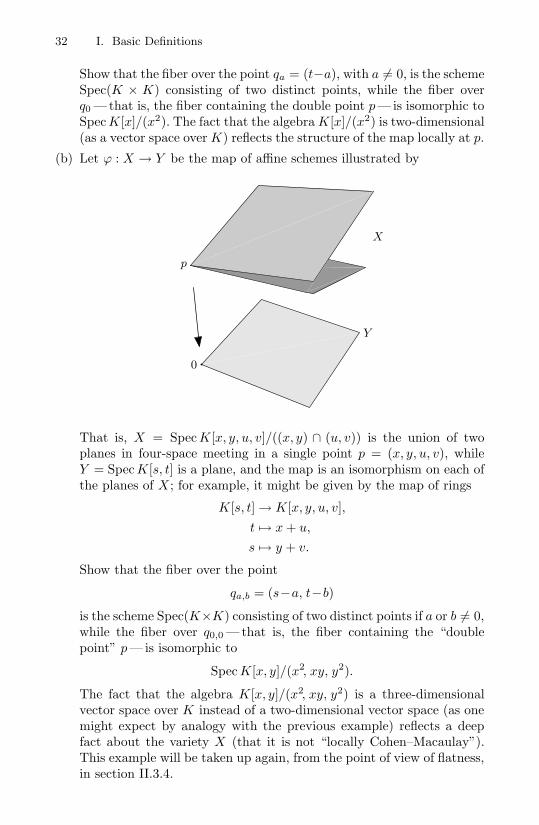
32 I. Basic Definitions
Show that the fiber over the point qa = (t−a), with a = 0, is the schemeSpec(K × K) consisting of two distinct points, while the fiber overq0 — that is, the fiber containing the double point p — is isomorphic toSpec K[x]/(x2). The fact that the algebra K[x]/(x2) is two-dimensional(as a vector space over K) reflects the structure of the map locally at p.
(b) Let ϕ : X → Y be the map of affine schemes illustrated by
0
p
X
Y
That is, X = Spec K[x, y, u, v]/((x, y) ∩ (u, v)) is the union of twoplanes in four-space meeting in a single point p = (x, y, u, v), whileY = Spec K[s, t] is a plane, and the map is an isomorphism on each ofthe planes of X ; for example, it might be given by the map of rings
K[s, t] → K[x, y, u, v],t → x + u,
s → y + v.
Show that the fiber over the point
qa,b = (s−a, t−b)
is the scheme Spec(K×K) consisting of two distinct points if a or b = 0,while the fiber over q0,0 — that is, the fiber containing the “doublepoint” p — is isomorphic to
Spec K[x, y]/(x2, xy, y2).
The fact that the algebra K[x, y]/(x2, xy, y2) is a three-dimensionalvector space over K instead of a two-dimensional vector space (as onemight expect by analogy with the previous example) reflects a deepfact about the variety X (that it is not “locally Cohen–Macaulay”).This example will be taken up again, from the point of view of flatness,in section II.3.4.

I.2 Schemes in General 33
I.2.4 The Gluing Construction
Using the notion of morphism, we can construct more complicated schemes(for example, nonaffine schemes) by identifying simpler schemes along opensubsets. This is a basic operation, called the gluing construction.
Suppose we are given a collection of schemes XαI , and an open setXαβ in Xα for each β = α in I. Suppose also that we are given a family ofisomorphisms of schemes
ψαβ : Xαβ → Xβα for each α = β in I,
satisfying the conditions ψβα = ψ−1αβ for all α and β,
ψαβ(Xαβ ∩ Xαγ) = Xβα ∩ Xβγ for all α, β, γ,
and the compatibility condition
ψβγ ψαβ |(Xαβ∩Xαγ) = ψαγ |(Xαβ∩Xαγ).
Under these circumstances we may define a scheme X by gluing the Xα
along the ψαβ in an obvious way— that is to say, there exists a (unique)scheme X with a covering by open subschemes isomorphic to the Xα suchthat the identity maps on the intersections Xα ∩ Xβ ⊂ X correspond tothe isomorphisms ψαβ .
This construction can be used, for example, to define projective schemesout of affine ones. Another use is in the theory of toric varieties; see, forexample, Kempf et al. [1973].
In these and indeed in almost all applications, we don’t really need togive the maps ψαβ explicitly: we are actually given a topological space |X |and a family of open subsets |Xα|, each endowed with the structure of anaffine scheme— that is, with a structure sheaf OXα — in such a way thatOXα(Xα∩Xβ) is naturally identified with OXβ
(Xα∩Xβ). For example, theymight both be given as subsets of a fixed set. Under these circumstancesit is immediate that the conditions of Corollary I-14 are satisfied, so thatthere is a uniquely defined sheaf OX on X extending all the OXα . The pair(|X |, OX) is then a scheme.
Probably the simplest example of this is the definition of affine spaceAn
S over an abitrary scheme S. To begin with, for any affine scheme X =Spec R we define affine n-space over X to be simply Spec R[x1, . . . , xn];this is denoted by either An
X or AnR. (The geometry of affine spaces and
their subschemes will be taken up in Chapter II.) Next, we note that anymorphism X → Y of affine schemes induces a natural map An
X → AnY . As
a consequence, we may apply the gluing construction as follows: If S is anarbitrary scheme covered by affine schemes Uα = Spec Rα, we define affinespace An
S over S to be the union of the affine spaces AnUα
, with the gluingmaps induced by the identity maps on Uα ∩ Uβ.
We will see two other ways of defining affine space AnS over an arbitrary
base S in Exercises I-47 and I-54 below.

34 I. Basic Definitions
The following exercise illustrates some of the dangers of the gluing con-struction: we can, by inappropriate (but legal) gluing, create schemes thatdo not arise in any geometric setting.
Exercise I-44. Put Y = Spec K[s] and Z = Spec K[t]. Let U ⊂ Y be theopen set Ys and let V ⊂ Z be the open set Zt. Let ψ : V → U be theisomorphism corresponding to the map
OY (U) = K[s, s−1] → K[t, t−1] = OZ(V )
sending s to t, and let γ be the map sending s to t−1. Let X1 be the schemeobtained by gluing together Y and Z along ψ, and let X2 be the schemeobtained by gluing along γ instead.
Show that X1 is not isomorphic to X2. In fact, X2 is the scheme cor-responding to the projective line P1
K (which we will describe in the nextsection), while X1 is the affine space with a doubled origin:
In Chapter III we will introduce a condition, called separatedness, thatwill preclude schemes such as this X1.
Projective Space. An important example of a scheme constructed bygluing is projective n-space over a ring R, denoted Pn
R. It is made by gluingn + 1 copies of affine space
AnR = Spec R[x1, . . . , xn]
over R. An extensive treatment of projective schemes will begin in ChapterIII. Here we will use the idea only as an illustration of gluing.
The construction is exactly parallel to the classical construction of pro-jective space as a variety over a field. Although not logically necessary, itis convenient to work as follows. Start with the polynomial ring in n + 1variables R[X0, . . . , Xn] and form the localization
A := R[X0, X−10 , . . . , Xn, X−1
n ].
Recall that the ring A has a natural grading, that is, a direct-sum decom-position (as an abelian group) into subgroups A(n), for n ∈ Z, such that
A(n)A(m) ⊂ A(m+n);
here A(n) is spanned by monomial rational fractions of degree n. In par-ticular, the degree 0 part A(0) is a subring of A. Now take the rings of ourdefining affine covering to be R-subalgebras of A(0), the i-th subring beingthe subalgebra Ai consisting of all polynomials P/X
deg(P )i , where P is a
homogeneous element of R[x0, . . . , xn]. Clearly, Ai is generated over R bythe n algebraically independent elements
X0/Xi, . . . , Xi/Xi, . . . , Xn/Xi,

I.3 Relative Schemes 35
where the hat denotes as usual an element omitted from the list. Ai is thusisomorphic to the polynomial ring in n variables over R. Further, for i = jwe have
Ai[(Xj/Xi)−1] = Aj [(Xi/Xj)−1]
as subsets of A; both may be described as the subalgebra of all degree0 elements having denominator of the form Xa
i Xbj . If we use the identity
maps as gluing maps, the compatibility conditions are obvious.If X = Spec R is an affine scheme, we will often write Pn
X instead of PnR,
and refer to the space as projective space over X. Any morphism X → Yof affine schemes induces a natural map Pn
X → PnY . As a consequence, we
may apply the gluing construction again to define projective space PnS over
an arbitrary scheme S as well. This is straightforward: if S is covered byaffine schemes Uα = Spec Rα, we define projective space Pn
S to be the unionof the projective spaces Pn
Uα, with the gluing maps induced by the identity
maps on Uα ∩ Uβ.
I.3 Relative Schemes
I.3.1 Fibered Products
There is an extremely important generalization of the idea of preimage ofa set under a function in the notion of the fibered product of schemes. Toprepare for the definition, we first recall the situation in the category ofsets.
The fibered product of two sets X and Y over a third set S — that is, ofa diagram of maps of sets
X
Yψ S
ϕ
is by definition the set
X ×S Y = (x, y) ∈ X × Y : ϕx = ψy.The fibered product is sometimes called the pullback of X (or of X → S)to Y. This construction generalizes several more elementary ones in a veryuseful way:
If S is a point, it gives the usual direct product.If X, Y are both subsets of S and ϕ,ψ are the inclusions, it gives the
intersection.If Y ⊂ S and ψ is the inclusion, it gives the preimage of Y in X.If X = Y, it gives the set on which the maps ϕ,ψ are equal, the equalizer
of the maps.

36 I. Basic Definitions
Exercise I-45. Check these assertions!
Note that X ×S Y comes with natural projection maps to X and Ymaking the diagram
X ×S Y X
Y
ψ S
ϕ
commute. Indeed, the set X×S Y may be defined by the following universalproperty: among all sets Z with given maps to X and Y making the diagram
Z X
Y
ψ S
ϕ
commute, X ×S Y with its projection maps is the unique “most efficient”choice in the sense that, given the diagram with Z above, there is a uniquemap Z → X ×S Y making the diagram
Z
X ×S Y
X
Y ψ
S
ϕ
commute.In the category of schemes we simply define the fibered product to be a
scheme with this universal property— the universal property guarantees inparticular that such a thing, with its projections to X and Y, will be unique.We can then define products, intersections, preimages, and equalizers interms of the fibered product! However, this begs the question of whetherany such object as the fibered product exists in the category of schemes. Itdoes, and we will now describe the construction.
First, we treat the affine case. Recall that the category of affine schemes isopposite to the category of commutative rings, by Corollary I-41. Therefore,if we have schemes
X = Spec A, Y = Spec B, S = Spec R,
where X and Y map to S (so that A and B are R-algebras), we must definethe fibered product X ×S Y to be
X ×S Y = Spec(A ⊗R B).

I.3 Relative Schemes 37
This is because the natural diagram
A ⊗R B A
B
R
ϕ
has, in an obvious sense, the opposite universal property to the one desiredfor the fibered product. In fancy language, the tensor product is a fiberedcoproduct, or fibered sum, in the category of commutative rings.
To check that this definition is reasonable, one may note that in thesituation where Y is a closed subscheme of S defined by an ideal I, so thatB = R/I, we have A ⊗R B = A/IA. Thus X ×S Y = Spec A/IA is thesame as the preimage of Y in X, as previously defined.
Exercise I-46. A few simple special cases are a great help when comput-ing fibered products. Prove the following facts directly from the universalproperty of the tensor product of algebras:
(a) For any R-algebra S we have R ⊗R S = S.
(b) If S, T are R-algebras and I ⊂ S is an ideal, then
(S/I) ⊗R T = (S ⊗R T )/(I ⊗ 1)(S ⊗R T ).
(c) If x1, . . . , xn, y1, . . . , ym are indeterminates then
R[x1, . . . , xn] ⊗R R[y1, . . . , ym] = R[x1, . . . , xn, y1, . . . , ym].
Use these principles to solve the remainder of this exercise.
(d) Let m, n be integers. Compute the fibered product
Spec Z/(m) ×Spec Z Spec Z/(n).
(e) Compute the fibered product Spec C ×Spec R Spec C.
(f) Show that for any polynomial rings R[x] and R[y] over a ring R, wehave
Spec R[x] ×SpecR Spec R[y] = Spec R[x, y].
Note that in example (d) the underlying set of the fibered product is thefibered product of the underlying sets, but this is not true in (e) and (f).
(g) Consider the ring homomorphisms
R[x] → R; x → 0
andR[x] → R[y]; x → y2.
Show that with respect to these maps we have
Spec R[y] ×SpecR[x] Spec R = Spec R[y]/(y2).

38 I. Basic Definitions
In the general case, we cover S by affine schemes Spec Rρ, and covertheir preimages in X and Y by affine schemes Spec Aρα and Spec Bρβ ,respectively, so that in a suitable sense the diagram
X
Yψ S
ϕ
is covered by diagrams of the form
Spec Aρα
Spec Bρβψρβ
Spec Rρ
ϕρα
Of course, we already know that the fiber product of this last diagramis Spec(Aρα ⊗Rρ Bρβ). Using the idea of gluing explained at the end of thepreceding section, it is easy but tedious to check that these schemes agree onoverlaps and patch together to form the scheme X×SY as required; we omitthe computation. A different approach will be sketched in section VI.2.1.
One immediate use of the notion of product is an alternative descriptionof affine space An
S over a scheme S:
Exercise I-47. Let S be any scheme. Let AnZ = Spec Z[x1, . . . , xn] be
affine space over Spec Z, as defined above (this scheme will be discussedin detail in the next chapter). Show that affine space An
S over S may bedescribed as a product: An
S = AnZ ×Spec Z S.
We can also use the fibered product to define the fiber of a morphismψ : Y → X over an arbitrary point of arbitrary schemes: if p is a pointof X corresponding to a prime ideal p of R, then the fiber of ψ over p isthe fibered product of Y and the one-point scheme Spec κ(p). In the casewhere X and Y are affine — say, Y = Spec T and X = Spec R —we get
ψ−1(p) = Spec κ(p) ×X Y = Spec(Rp/pp ⊗R T ) = Spec(Rp/pp ⊗R T/pT )
as a point set; this is the set of primes of T whose preimages in R are equalto p. More generally, we define the preimage, or inverse image of a closedsubscheme X ′ of X under ψ to be the fibered product X ′ ×X Y.
Just as in the affine case treated above, the preimage ψ−1X ′ of X ′ is aclosed subscheme of Y . Using the OX -algebra structure on OY , the idealsheaf of the preimage may be written as Iψ−1X′ = IX′ · OY .
Another typical use of the fibered product is in studying the behavior ofvarieties under extension of a base field (one usually speaks in this contextof a “base change” rather than a fibered product). In this setting, of whichwe will see some examples in the following chapter, the notion is responsible

I.3 Relative Schemes 39
for the great flexibility and convenience of the theory of schemes in handlingarithmetic questions.
As in examples (b) and (c) of Exercise I-46, the set of points of the fiberedproduct of schemes X ×S Y is usually not equal to the fibered product (inthe category of sets) of the sets of points of X and Y. This is no terriblepathology but simply reflects the fact that the theory of functions f(x, y)of two variables is much richer than the theory of functions of the formg(x)h(y). In any case, the definitions of Chapter VI provide a viewpointfrom which this oddity disappears.
I.3.2 The Category of S-Schemes
Just as in the case of sets, we can use the fibered product to define anabsolute product by taking S to be a terminal object in the category ofschemes— that is, a scheme such that every scheme has a unique map to S.By Exercise I-42 the terminal object in the category of schemes is Spec Z.However, the absolute product has some rather surprising properties. Wehave already seen in Exercise I-46(d) cases (when m and n are relativelyprime) where the product in this sense of nonempty sets may be empty!There are other peculiarities as well: for example, the dimension of anirreducible scheme can be defined as the Krull dimension of the coordinatering of any of its affine open sets. One might expect the product
X × Y = X ×SpecZ Y
of two schemes to have dimension equal to the sum of the dimensions of Xand Y. But in fact we have the result in the next exercise.
Exercise I-48. Show that if X = Spec Z[x] and Y = Spec Z[y], then
dim X × Y = dimX + dimY − dimSpec Z = dimX + dimY − 1.
This oddity and many like it can be eliminated by a simple but convenientgeneralization of our definitions: we often wish to work with schemes X overa given field (or ring) K, or K-schemes. Of course, we will then use onlymorphisms that respect this structure. Informally, this just means that weconsider X together with a K-algebra structure on OX(X) and morphismsrespecting these structures. In this category, Spec K is the terminal objectand the absolute product is the fibered product over SpecK. If K is afield, the product in the category of K-schemes behaves more in accordwith elementary geometric intuition. For example:
Exercise I-49. Let K be a field. If X and Y are nonempty K-schemes,then the product X × Y = X ×SpecK Y in the category of K-schemes isnonempty.
Further, in this case the dimension of Spec K is 0, and one can checkthat for schemes built up from spectra of finitely generated K-algebras thedimension of products is additive, as it should be.

40 I. Basic Definitions
In order to accommodate families of schemes, we may extend this notiona little further. A K-algebra structure on OX(X) is nothing but a homo-morphism of rings from K to OX(X), and by Theorem I-40 this is exactlythe same as a map X → Spec K. Replacing Spec K by an arbitrary schemeS, we define a scheme over S, or S-scheme, to be a scheme X togetherwith a morphism X → S. We may think of a scheme over S informallyas a family of schemes “parametrized by points of S”— for each point ofS we have the fiber over that point. A morphism of schemes over S (orS-morphism) is a commutative diagram
X Y
S
If X and Y are schemes over S, then we write MorS(X, Y ) for the set ofS-morphisms. Note that the fibered product X ×S Y of schemes over S isprecisely the ordinary direct product in the category of schemes over S.
As usual, if S = Spec R is affine, we will use the terms “R-scheme” and“the category of R-schemes” interchangeably with “S-scheme” and “thecategory of S-schemes”.
Introducing the category of schemes over S may seem to add a layer ofcomplication, but in reality it more often removes one. For example, if wewant to do classical algebraic geometry over the complex numbers in schemelanguage, it is necessary to work in the category of schemes over C. To seethat this is so, note that in any reasonable sense the point Spec C shouldhave no nontrivial automorphisms, and the scheme Spec C[x]/(x2 +1) con-sisting of a pair of points should have automorphism group Z/(2). Thisis in fact the case in the category of schemes over C. In the categoryof all schemes, however, the automorphism group of the point Spec C ishuge: it is the Galois group of C over Q, and the automorphism group ofSpec C[x]/(x2 +1) is worse. Thus, working in the category of schemes overC removes the (presumably unwanted) extra structure of the Galois groupGal(C/Q).
Exercise I-50. Find the automorphism groups of the schemes X1 and X3
of Exercise I-20 in the category of schemes over C.
I.3.3 Global Spec
If S = Spec R is an affine scheme, an affine S-scheme is simply the spectrumof an R-algebra. We will now extend this construction to describe analogousobjects in the category of S-schemes for arbitrary S.
To begin with, for any scheme S we define a quasicoherent sheaf of OS-algebras. This is, as you might expect, a sheaf F of OS-algebras, suchthat for any affine open U = Spec R ⊂ S and distinguished open subset

I.3 Relative Schemes 41
U ′ = Spec Rf ⊂ U, we have
F (U ′) = F (U) ⊗R OS(U ′) = F (U) ⊗R Rf
as R = OS(U)-algebras. We then associate to any quasicoherent sheaf Fof OS-algebras on a scheme S a scheme X = Spec F, together with astructure morphism X → S, such that in case S = Spec R is affine weget simply X = Spec F (S) together with the structure morphism X → Sinduced by the R = OS(S)-algebra structure on F (S).
There are a couple ways to do this. One is simply to use the gluingconstruction again: we cover S by affine open subsets Uα = Spec Rα, anddefine X to be the union of the schemes Spec F (Uα), with attaching mapsinduced by the restrictions maps F (Uα) → F (Uα ∩ Uβ). This works, butit’s a mess to verify that the resulting space Spec F is independent of thechoice of cover, and has the further drawback that it can be awkward todescribe the set of points of Spec F. We will give here instead an alternativeconstruction.
We start with a definition: given a quasicoherent sheaf F of OS-algebras,we define a prime ideal sheaf in F to be a quasicoherent sheaf of idealsI F, such that for each affine open subset U ⊂ S, the ideal I (U) ⊂F (U) is either prime or the unit ideal. (Observe that for any affine schemeX, the points of X are simply the prime ideal sheaves of OX .) Now, we willdefine X = Spec F in three stages, as we did the spectrum of a ring. First,as a set, X is the set of prime ideal sheaves in F. Second, as a topologicalspace: for every open U ⊂ S (not necessarily affine) and section σ ∈ F (U),let VU,σ ⊂ X be the set of prime ideal sheaves P ⊂ F such that σ /∈ P(U);take these as a basis for the topology. Finally, we define the structure sheafOX on basis open sets by setting
OX(VU,σ) = F (U)[σ−1].
As for the morphism f : X → S: as a set, we associate to a prime idealsheaf P ⊂ F its inverse image in OS → F ; and the pullback map onfunctions
f# : OS(U) → OX(f−1(U)) = F (U)
is just the structure map OS → F on U.
Exercise I-51. Show that the points of an affine scheme X are in one-to-one correspondence with the set of prime ideal sheaves in OX .
Exercise I-52. Show that if f : Y → X is a morphism and P is a primeideal sheaf of OY , then f∗(P) is a prime ideal sheaf in f∗OY .
Exercise I-53. Show that if f : Y → X is a morphism, the map on setscorresponding to f sends P ⊂ OY to (f#)−1(f∗(P)) ⊂ OX .
The simplest example of global Spec gives us yet another constructionof affine space over an arbitrary scheme S:

42 I. Basic Definitions
Exercise I-54. Let S be any scheme. Show that affine space AnS over S
may be constructed as a global Spec:
AnS = Spec
(Sym(O⊕n
S )).
I.4 The Functor of Points
One of the intriguing things about schemes is precisely that they have somuch structure that is not conveyed by their underlying sets, so that thefamiliar operations on sets such as taking direct products require vigilantscrutiny lest they turn out not to make sense. It is therefore remarkable thatmany of the set-theoretic ideas can be restored through a simple device,the functor of points. This point of view, while initially adding a layer ofcomplication to the subject, is often extremely illuminating; as a result itand its attendant terminology have become pervasive. We will give a briefintroduction to the necessary definitions here and use them occasionally inthe following chapters before returning to them in detail in Chapter VI.
We start with the observation that the points of a scheme do not ingeneral look anything like one another: we have nonclosed points as well asclosed ones; and if we are working over a non-algebraically closed field, theneven closed points may be distinguished by having different residue fields.Similarly, if we are working over Z, different points may have residue fieldsof different characteristic; and if we extend the notion of point to “closedsubscheme whose underlying topological space is a point,” we have an evengreater variety. And, of course, a morphism between schemes will not at allbe determined by the associated map on underlying point sets.
There is, however, a way of looking at a scheme— via its functor ofpoints — that reduces it in effect to a set. More precisely, we may think ofa scheme as an organized collection of sets, a functor on the category ofschemes, on which the familiar operations on sets behave as usual. In thissection we will examine this functorial description. A big payoff is that wewill see the category of schemes embedded in a larger category of functors,in which many constructions are much easier. The advantage of this issomething like the advantage in analysis of working with distributions, notjust ordinary functions; it shifts the problem of making constructions inthe category of schemes to the problem of understanding which functorscome from schemes. Further, many geometric constructions that arise inthe category of schemes can be extended to larger categories of functors ina useful way.
To introduce the notion of the functor of points, we start out in a generalcategorical setting. To begin with, in many categories whose objects aresets with additional structure, the underlying set |X | of an object X maybe described as the set of morphisms from a universal object to X ; forexample:

I.4 The Functor of Points 43
(a) In the category of differentiable manifolds, if Z is the manifold consist-ing of one point, then for any manifold X we have |X | = Hom(Z, X).
(b) In the category of groups, for any group X we have |X | = Hom(Z, X).
(c) In the category of rings with unit and unit-preserving homomorphisms,if we set Z = Z[x], then for any ring X with unit we have |X | =Hom(Z, X).
In general, for any object Z of a category X the association
X → HomX (Z, X)
defines a functor ϕ from the category X to the category of sets. As indi-cated in the first paragraph above, however, it is not really satisfactory tocall the set ε(X) = HomX (Z, X) the set of points of the object X unlessthis functor is faithful — that is, unless for any pair of objects X1 and X2
of X a morphismf : X1 → X2
is determined by the map of sets
f ′ : HomX (Z, X1) → HomX (Z, X2).
It may not always be possible to satisfy this condition. For example, let(Hot) be the category of CW -complexes, where Hom(Hot)(X, Z) is the setof homotopy classes of continuous maps from X to Z. If Z is the one-pointcomplex, then
Hom(Hot)(Z, X) = π0(X)
the set of connected components of X, and this does not give a faithfulfunctor. Nor is it possible to chose a better object Z. Likewise, in thecategory of schemes, there is no one object Z that will serve in this capacity.
Grothendieck’s ingenious idea was to remedy this situation by consid-ering not just one set Mor(Z, X) but all at once! That is, we associate toeach scheme X the “structured set” consisting of all the sets Mor(Z, X), to-gether with, for each morphism f : Z → Z ′, the mapping from Mor(Z ′, X)obtained by composing with f .
To put this more formally, the functor of points of a scheme X is the“representable” functor determined by X ; that is, the functor
hX : (schemes) → (sets),
where (schemes) and (sets) represent the category of schemes with thearrows reversed and the category of sets, respectively; hX takes each schemeY to the set
hX(Y ) = Mor(Y, X)
and each morphism f : Y → Z to the map of sets
hX(Z) → hX(Y )
44 I. Basic Definitions
defined by sending an element g ∈ hX(Z) = Mor(Z, X) to the compositiong f ∈ Mor(Y, X). The reason for the name “representable functor” is thatwe say this functor is represented by the scheme X. The set hX(Y ) is calledthe set of Y -valued points of X (if Y = Spec T is affine, we will often writehX(T ) instead of hX(Spec T ) and call it the set of T -valued points of X).
To introduce one more layer of abstraction, note that this constructiondefines a functor
h : (schemes) → Fun((schemes), (sets))
(where morphisms in the category of functors are natural transformations),sending
X → hX
and associating to a morphism f : X → X ′ the natural transformationhX → hX′ that for any scheme Y sends g ∈ hX(Y ) = Mor(Y, X) to thecomposition f g ∈ hX′(Y ) = Mor(Y, X ′).
Of course, when we want to work with schemes over a given base S, weshould take morphisms over S as well. The situation is completely analo-gous to that above: we describe in this way a functor
X → hX
from the category of S-schemes to the category
Fun((S-schemes), (sets)).
The apparently abstract idea of the functor of points has its root in thestudy of solutions of equations. Let X = Spec R be an affine scheme, whereR = Z[x1, x2, . . .]/(f1, f2, . . .). If T is any other ring (one should think ofT = Z, Z/(p), Z(p), Z(p), Qp, R, C, and so on), then a morphism fromSpec T to Spec R is the same as a ring homomorphism from R to T, andthis is determined by the images ai of the xi. Of course, a set of elementsai ∈ T determines a morphism in this way if and only if they are solutionsto the equations fi = 0. We have shown that
hX(T ) =
sequences of elements a1, . . . ∈ T thatare solutions of the equations fi = 0
.
Similarly, if X is an arbitrary scheme, so that X is the union of affineschemes Xa meeting along open subsets, then a map from an affine schemeY to X may be described by giving a covering of Y by distinguished affineopen subsets Yfa and maps from Yfa to Xa for each a, agreeing on open sets(some of the Yfa may, of course, be empty). Thus an element of hX(Y ) maybe described even in this general context as a set of solutions to systems ofequations, corresponding to some of the Xa, with compatibility conditionssatisfied by the solutions on the sets where certain polynomials are non-zero.
Even with this interpretation, the notion of the functor of points mayseem an arid one: while we can phrase problems in this new language,

I.4 The Functor of Points 45
it’s far from clear that we can solve them in it. The key to being able towork in this setting is the fact that many apparently geometric notionshave natural extensions from the category of schemes to larger categoriesof functors. Thus, for example, we can talk about an open subfunctor ofa functor, a closed subfunctor, a smooth functor, the tangent space to afunctor, and so on. These notions will be developed in Chapter VI, wherewe will also give a better idea of how they are used.
In this chapter we have used the word “point” in two different ways: wehave both the points of a scheme X, and, for any scheme Y, the set ofY -valued points of X. It is important not to let this double usage causeconfusion. The two notions are of course very different: for example, ifY = Spec L for some finite extension L of Q, then we have a map
Y -valued points of X −→ |X |but this map is in general neither injective or surjective: the image will bethe subset of points p ∈ X whose residue field κ(p) is a subfield of L, and thefiber of the map over such a point p will be the set of ring homomorphismsfrom κ(p) to L. Another distinction is that while the set |X | of points of Xis absolute, the set of Y -valued points is relative in the sense that it maydepend on the specification of a base scheme S and the structure morphismX → S. Finally, in case S = Spec K, the set of K-valued points of X —that is, the subset of points p ∈ X such that κ(p) = K — is often calledthe set of K-rational points of X.
Each of the two notions of “point” has some (but not all) of the propertieswe might expect from the behavior of points in the category of sets. Forexample, the set of Y -valued points of a product X1×X2 is the product ofthe sets of Y -valued points of X1 and X2. However, it is not the case thatthe set of Y -valued points of a union X = U ∪ V is the union of the setsof Y -valued points of U and V (for example, the identity map X → X isan X-valued point of X not in general contained in U or V ). By contrast,exactly the opposite situation holds for the set |X | of points of a schemeX in the ordinary sense.
We have now outlined the basic definitions in the theory of schemes. Inthe next chapter we will give many examples, from which the reader mayform some idea of the “look and feel” of schemes.

IIExamples
II.1 Reduced Schemes over Algebraically ClosedFields
We will start our series of examples with the one that the concept of schemeis intended to generalize: the classical notion of an affine variety over analgebraically closed field K. In our present context, this means consideringschemes of the form Spec R, where R is the coordinate ring of a variety X —that is, a finitely generated, reduced algebra over K. (Recall that “reduced”means nilpotent-free.) Spec R is sometimes called the scheme associated tothe variety X : such schemes are sometimes referred to just as varieties. Inlater sections we will consider the ways in which schemes may differ fromthis basic model.
The K-scheme associated to an affine variety over an algebraically closedfield K is an equivalent object to the variety; either one determines andis determined by its coordinate algebra, which is the same for both. Butalready in this case, classical notions such as the intersection of varietiesand the fibers of maps are given a more precise meaning in the theory ofschemes. We will see examples of this phenomenon in this and succeedingsections.
II.1.1 Affine Spaces
We start with the scheme AnK := Spec K[x1, . . . , xn], with K an alge-
braically closed field. This scheme is called affine n-space over K.

48 II. Examples
We will make use of a standard but nontrivial result from algebra, a formof Hilbert’s Nullstellensatz; see Eisenbud [1995], for example.
Theorem II-1 (Nullstellensatz). Let K be any field. If m is a maximalideal of a polynomial ring K[x1, . . . , xn] (or, geometrically, p is a closedpoint of any subvariety of an affine space over a field K), then
K[x1, . . . , xn]/m = κ(p)
is a finite-dimensional vector space over K.
In our case, with K algebraically closed, this implies that κ(p) = K.Thus, writing λi for the image of xi in κ(p), we see that
m = (x1 − λ1, . . . , xn − λn).
In this way the closed points of AnK correspond to n-tuples of elements of K,
as one should expect. We will sometimes refer to “the point (λ1, . . . , λn)”instead of “the point [(x1 − λ1, . . . , xn − λn)].”
To begin with dimension 1, the affine line
A1K = Spec K[x]
looks almost exactly like its classical counterpart, the algebraic varietyalso called the affine line. It contains one closed point for each value λ ∈K. The Zariski topology on the set of closed points is the same as theclassical Zariski topology on the variety: the open sets are the complementsof finite sets. The scheme A1 differs from the variety only in that the schemecontains one more point, called the generic point of A1, corresponding tothe ideal (0).
(0)(x) (x − λ)
The closure of the point (0) is all of A1K , so that the closed subsets of A1
K
are exactly the finite subsets of A1K − (0).
The affine plane A2K = Spec K[x, y] is also similar to its counterpart
variety, but now the additional points of the scheme are more numerous andbehave in more interesting ways. We have as before closed points, comingfrom the maximal ideals (x − λ, y − µ), which correspond to the points(λ, µ) in the ordinary plane. There are now, however, two types of nonclosedpoints. To begin with, for each irreducible polynomial f(x, y) ∈ K[x, y] wehave a point corresponding to the prime ideal (f) ⊂ K[x, y], whose closureconsists of the point itself and all the closed points (λ, µ) with f(λ, µ) = 0.The point (f) is called the generic point of this set; more generally, anypoint in a scheme is called the generic point of its closure. As compared tothe variety A2
K , we have added one more point for every irreducible planecurve. This new point lies in the closure of (the set of closed points on)that curve, and its closure contains this set of closed points. Finally, we

II.1 Reduced Schemes over Algebraically Closed Fields 49
have as before a point corresponding to the zero ideal, the generic point ofA2
K , whose closure is all of A2K .
(0) generic point of A2
(x) generic point of the x-axis
(x−λ, y−µ)
(f(x, y)) generic point of the curve(y)
Since K[x, y] = K[x] ⊗K K[y], we have by definition
A2K = A1
K ×SpecK A1K .
Even here, though it’s clear that the fibered product is the correct notion ofproduct, the set of points of the fibered product is not the fibered productof the sets of points of the factors.
The situation with the affine spaces AnK =Spec K[x1, . . . , xn] is a straight-
forward extension of the last case: geometrically, we can see the scheme AnK
as the classical affine n-space, with one point pΣ added for every positive-dimensional irreducible subvariety Σ of n-space. As above, pΣ will lie inthe closure of the locus of closed points in Σ and contain in its closure allthese points, as well as the generic points of the subvarieties of Σ.
More generally, suppose X ⊂ AnK is any affine variety, with ideal I ⊂
K[x1, . . . , xn] and coordinate ring R = K[x1, . . . , xn]/I. We can associateto X the affine scheme Spec R; the quotient map K[x1, . . . , xn] → R ex-presses this as a subscheme of An
K . This scheme is, as in the case of AnK
itself, just like the variety X except that we have added one new genericpoint pΣ for every positive-dimensional irreducible subvariety Σ ⊂ X.
Fibers, and more generally preimages, are among the most common waysthat schemes other than varieties may arise even in the context of classicalgeometry.
Exercise II-2. Consider the map of the affine line Spec K[x] to itself in-duced by the ring homomorphism K[x] → K[x] mapping x to x2. Show

50 II. Examples
that the scheme-theoretic fiber over the point 0 is the subscheme of theline defined by the ideal (x2).
Among all schemes, those associated to affine varieties over algebraicallyclosed fields may be characterized as spectra of rings R that are
– finitely generated
– reduced algebras
– over a field
– that is algebraically closed.
To get a sense of what more general schemes look like, and what theyare good for, we will in the remainder of this section and the next considerwhat may happen if we remove these four restrictions. We will considerprimarily examples in which exactly one of the hypotheses fails, since anunderstanding of these basic cases will enable one to understand the generalcase; we will occasionally mention more complex examples in exercises.
II.1.2 Local Schemes
Our first collection of examples of schemes other than varieties is providedby the spectra of local rings, called local schemes. The examples we willconsider here are spectra of rings that are reduced algebras over an alge-braically closed field but not, in general, finitely generated. Local schemesare for the most part technical tools in the study of other, more geomet-ric schemes; they are often used to focus attention on the local structureof an affine scheme. The extra points we have added to classical varietiesshow up even more strikingly in the following examples, where in each casethere is only one closed point. It would, of course, be a mistake to try topicture these schemes as geometric objects with just one point. Rather,they should be seen as germs of varieties. The phenomenon of having onlyone closed point is not some novelty invented by algebraists but is already

II.1 Reduced Schemes over Algebraically Closed Fields 51
present if one considers such a familiar object as the germ of a point xon a complex analytic manifold; here one pictures a “sufficiently small”neighborhood of x, in which, for example, each curve through x can beplainly distinguished, even though no other definite points beside x belongto every neighborhood. We will see that the same kind of picture is validfor the spectrum of a local ring.
Consider first the localization K[x](x) of the ring K[x] at the maximalideal (x), and let X = Spec K[x](x). The space |X | has only two points:the closed point corresponding to the maximal ideal (x), and the openpoint corresponding to (0), which contains the point (x) in its closure. Theinclusion of K[x] in K[x](x) induces a map X → A1
K , so that we may thinkof X as a subscheme of A1
K (though |X | is neither open nor closed in |A1K |).
The subscheme X is “local” in that it is the intersection of all the opensubsets of A1
K containing the point (x); so that, for example, the regularfunctions on X are exactly the rational functions on A1
K regular at the point(x) —that is, they are the elements of OA1
K(U) for some neighborhood U
of the point 0 = (x) in A1K . In these senses, X is the germ of A1
K at theorigin.
Next, consider the scheme X = Spec R, where R = K[x, y](x,y) is thelocalization of K[x, y] at the maximal ideal (x, y) corresponding to thepoint (0, 0). As in the previous example, we have a map X → A2
K , in termsof which we can think of X as the intersection of all open subschemes of A2
K
containing the closed point (0, 0). Again, X has only one closed point; butnow there are infinitely many nonclosed points, one for every irreduciblecurve in the plane passing through the origin. Subschemes of X are thusgerms at (0, 0) of subschemes of A2
K and X itself is the germ of A2K at the
origin.There are analogous constructions in An
K , and more generally for anysubscheme of An
K : if X = Spec K[x, . . . , xn]/I ⊂ AnK is the scheme asso-
ciated to the affine variety with ideal I ⊂ K[x, . . . , xn] and m = (x1−a1,. . . , xn−an) a maximal ideal corresponding to a closed point of X, we canconsider the scheme Spec K[x1, . . . , xn]m/Im as a germ of a neighborhoodof [m] in X. While we can talk about germs of functions on a space at apoint in many contexts, in scheme theory the germ is again a scheme in itsown right.
For some purposes, the local schemes introduced in this way are notlocal enough; the local ring of a scheme at a point still contains a lotof information about the global structure of the scheme. For example, thegerms of a nonsingular variety X at various closed points will not in generalbe isomorphic schemes1, although if Xan denotes the complex analyticvariety defined by the same equations (or indeed any analytic manifold),
1This has nothing to do with schemes but is already the case for varieties over C: forexample, it is so already for the general plane curve of degree d ≥ 4.

52 II. Examples
the germs of Xan at any two points are isomorphic. This phenomenonoccurs essentially because the open sets used to define the germs of X areso big. To get a more local picture within the setting of schemes, we canlook at the schemes associated to power series rings: for example, insteadof looking at the germ X = Spec K[x, y](x,y) of a neighborhood of theorigin in A2
K above, we can consider the scheme Y = Spec K[[x, y]]. As inthe previous case, this scheme has one closed point [(x, y)] and one genericpoint [(0)] whose closure is all of Y ; in addition, it has one point for everyirreducible power series
∑ai,jx
iyj in x and y. The maps
K[x, y] → K[x, y](x,y) → K[[x, y]]
give maps Y → X → A2K ; we think of the Y as a “smaller” neighborhood
of the origin than X. (Note, however, that X and Y are neither closedsubschemes nor open subschemes of A2
K .) For example, while the curvecorresponding to the prime ideal (y2−x3−x2) is irreducible in X, becausethe curve in A2
K defined by this equation is, the preimage in Y of this curveis the (nontrivial) union of two curves in Y , as long as the characteristic ofK is not 2, because x2 + x3 has the square root
u = x + 12x2 − 1
8x3 + · · ·in the power series ring. Thus we can factorize y2 − x3 − x2 as
y2 − x3 − x2 = (y − u)(y + u),
so the scheme Spec K[[x, y]]/(y2 − x3 − x2) is reducible. (See the figure onthe next page.)
Of course, Y must have “more” curves than X for such things to bepossible. The following exercise amplifies this fact.
Exercise II-3. (a) With u =√
x2 + x3 as above, what is the image of[(y−u)] in Spec K[x, y]? (Hint: it’s a prime ideal containing y2−x3−x2.)
(b) Show that the image of the point (y−∑n≥1 xn/n!) of Y is the generic
point of A2K .
In general, under the map Y → X above, the inverse image of a pointcorresponding to an irreducible curve C ⊂ A2
K consists of the set of analyticbranches of C at the origin. (See Walker [1950] or Brieskorn and Knorrer[1986] for further discussion of branches.)
Here is yet another important example of a local scheme. One problemwith the scheme Y above is that the points described in Exercise II-3(b)are extraneous from an algebraic point of view. To avoid this, we may workwith the spectrum Z of the ring H ⊂ K[[x, y]] of power series that satisfyalgebraic equations over K(x, y), the field of rational functions. Called theHenselization of X , the scheme Z sits in between Y and X in the sensethat we have a series of maps
Y → Z → X → A2K .

II.2 Reduced Schemes over Non-Algebraically Closed Fields 53
SpecK[x, y]/(y2−x3−x2) ⊂SpecK[x, y] is irreducible;
its preimageSpecK[[x, y]]/(y2−x3−x2)⊂ Spec K[[x, y]] is not.
The usefulness of this construction is that H is the union of algebras finitelygenerated over K, so that Z is the inverse limit of schemes coming fromordinary varieties. Geometrically, Z is the germ of A2
K in the etale topology,a concept we will not pursue here; see Artin [1971] for further information.
Exercise II-4. In the case K = C, how does the spectrum of the ring ofconvergent power series fit into this picture?
II.2 Reduced Schemes over Non-AlgebraicallyClosed Fields
We now consider what happens when we look at the spectrum of a finitelygenerated, reduced algebra over a field K that is not algebraically closed.The interest in such structures came originally from number theory, and,of course, it predates scheme theory very substantially! For example, thestudy of rational quadratic forms, an old subject in number theory, canbe thought of as the study of varieties over the rational numbers definedby a quadratic equation. Cubic forms in three variables over the rationalsstill make up a very active number-theoretic research topic, now mostlypursued through the theory of elliptic curves over Q. The basic objectsthemselves are varieties over Q (or schemes over Z, a situation we’ll returnto later), but in the course of handling them, number theorists frequentlymake use of all the base rings shown in the following diagram, along with

54 II. Examples
many intermediate fields and rings:
Z(p) Qp
Cp
Z(p)
Z
Q
R C
Fp
Fp
The theory of schemes provides a particularly flexible and convenient frame-work for handling these many changes of base. Also, a nice variety reducedmod p may suddenly become something nonreduced— something that re-quires the theory of schemes more fully (see for example Section II.4.4).
To start with the simplest case, consider A1R = Spec R[x]. Using the
Nullstellensatz we see that there are two kinds of maximal ideals in R[x]:those whose residue class field is R, which have the form (x−λ) for λ ∈ R,and those whose residue class field is C, which have the form (x2 +µx+ν),for µ and ν ∈ R with µ2 − 4ν < 0. The latter type of ideals may also bewritten in the form ((x − z)(x − z)), for z ∈ C not real. A closed pointof A1
R thus corresponds either to a real number or to a conjugate pair ofnonreal complex numbers. Finally, A1
R has again a unique nonclosed pointcorresponding to the prime (0), whose closure is all of A1
R .Next, we turn to the affine plane over R, A2
R = Spec R[x, y], and considera closed point given by a maximal ideal m of R[x, y]. Again by the Null-stellensatz the residue class field of m is either R or C, and the compositemap
R → R[x, y]/m ∼= (R or C)
is either the identity or the inclusion of R in C. Taking λ and µ to be theimages of x and y in C, we see that in the former case m = (x−λ, y−µ)corresponds to the ordinary point (λ, µ) in R2. But in the latter case mcorresponds to both (λ, µ) and (λ, µ); put differently, the map R[x, y] → Csending x, y to λ, µ has the same kernel as the one sending x, y to λ, µ sincethey differ by the automorphism of C over R.
It is not difficult to give generators for the maximal ideals describedabove. If R[x, y]/m ∼= R, then clearly m = (x−λ, y−µ). In the othercase, suppose first that λ is real. Then µ must satisfy an irreducible realquadratic polynomial equation y2 +ay+b = 0, so m contains the ideal(x−λ, y2+ay+b). But this last ideal is immediately seen to be prime (forexample, by factoring out x−λ first), so m = (x−λ, y2+ay+b). Of course,a similar result holds if the image of y is real.

II.2 Reduced Schemes over Non-Algebraically Closed Fields 55
Finally, suppose that µ and λ are both nonreal. Then m contains theirreducible polynomials f(x) and g(y) satisfied by µ and λ, but since g(y)factors as
g(y) = (y−µ)(y−µ)
in R[x]/(f(x)) ∼= C the ideal (f(x), g(y)) is not prime! The picture here,over the complex numbers, is as follows:
(λ, µ)(λ, µ)
(λ, µ)(λ, µ)
f(x) = 0
g(y) = 0
Im(µ)x−Im(λ) y = Im(µλ)
A line whose equationhas real coefficients
The loci defined by f(x) = 0 and g(y) = 0 are unions of two vertical andtwo horizontal lines, respectively, and intersect in the four points (λ, µ),(λ, µ), (λ, µ), and (λ, µ). But the polynomial
h(x, y) = Im(µ)x − Im(λ) y − Im(µλ)
defining the line joining the two points (λ, µ) and (λ, µ) has real coefficients.The ideal
(f(x), h(x, y)) = (g(y), h(x, y)) ⊂ R[x, y]
thus strictly contains the ideal (f(x), g(y)); and this ideal is the maximalideal m we seek, as one checks by working in
R[x] ∼= R[x, y]/(h) ∼= R[y]
(for these isomorphisms, note that (µ−µ) and (λ−λ) are both nonzero).In sum, then, the closed points of A2
R correspond either to points (λ, µ)of A2
C with λ and µ real, or to (unordered) pairs of points (z, w) and(z, w) ∈ A2
C with at least one of z, w not real. To put it another way, closedpoints of A2
R correspond to orbits of the action of complex conjugation onthe points of A2
C . (Note, in particular, that the closed points of A2R are not
ordered pairs of closed points of A1R !) Observe also that the residue field is

56 II. Examples
R at the points of A2R corresponding to points (λ, µ) with λ, µ real, while
at points of A2R corresponding to pairs of complex conjugate points of A2
C
the residue field is C.
Exercise II-5. Show that the nonclosed points of A2R are all either
(a) [(0)], whose closure is all of A2R , or
(b) the point [(f)] of A2R corresponding to an irreducible polynomial f ∈
R[x, y].
Those of type (b) may or may not remain irreducible in C[x, y], so thata nonclosed point (f) in A2
R will correspond either to a single nonclosedpoint in A2
C (if f remains irreducible in C[x, y]) or to two nonclosed pointsin A2
C (if f may be written as a product g g with g ∈ C[x, y]). The closedpoints in the closure of such a nonclosed point may be either of both typesabove or only of the second. Give examples with all these possibilities.
The situation in general follows the lines of these examples: if K is anyfield, K its algebraic closure, and G = Gal(K/K) the corresponding Galoisgroup, the points of An
K correspond to orbits of the action of G on the pointsof An
K (see, for example, Nagata [1962, Theorem 10.3]). The closed pointscorrespond to orbits of closed points, the orbits being finite. The residuefield at the point p corresponding to such an orbit, moreover, is isomorphicto the fixed field of the action on K of the subgroup Gp fixing a point of thatorbit. For example, the closed points of A1
Q correspond to algebraic numbersmodulo conjugacy; and for a prime number q ∈ Z the closed points of A1
Fq
correspond to the orbits of the Frobenius automorphism of the algebraicclosure of Fq = Z/(q) (namely, 0 and the orbits of the map a → aq on themultiplicative group K∗, which may be described as the inductive limit ofall cyclic groups of order prime to q or as the q-torsion-free part of Q/Z).
Exercise II-6. An inclusion of fields K → L induces a map AnL → An
K .Find the images in A2
Q of the following points of A2Q
under this map.
(a) (x−√2, y−√
2)
(b) (x−√2, y−√
3)
(c) (x−ζ, y−ζ−1), where ζ is a p-th root of unity, with p prime
(d) (√
2x−√3y)
(e) (√
2x−√3y−1)
Where feasible, draw pictures.
Exercise II-7. We say that a subscheme X ⊂ AnK is absolutely irreducible
or geometrically irreducible if the inverse image of X in AnK is irreducible.
(More generally, we say any K-scheme X is absolutely irreducible if thefiber product X ×SpecK Spec K is irreducible.) Classify the following sub-schemes of A2
Q = Spec Q[x, y] as reducible, irreducible but not absolutelyirreducible, or absolutely irreducible.

II.3 Nonreduced Schemes 57
(a) V (x2−y2)
(b) V (x2+y2)
(c) V (x2+y2−1)
(d) V (x+y, xy−2)
(e) V (x2−2y2, x3+3y3)
Finally, here is an example that combines the notions of local schemes andschemes over non-algebraically closed fields. Classically, a plane curve X ⊂A2
C was said to have a node at the origin if in some analytic neighborhoodof the origin the locus of complex points of Y consisted of two smooth arcsintersecting transversely at (0, 0). In the language of schemes, this is thesame as saying that the fiber product of X with the formal neighborhoodSpec C[[x, y]] → Spec C[x, y] = A2
C is isomorphic to Spec C[[u, v]]/(uv).Consider now a curve in the real plane X ⊂ A2
R . We say in this case thatX has a node at the origin if the corresponding complex curve
X ×SpecR Spec C ⊂ A2C
does. In this case, the formal neighborhood
X ×Spec R[x,y] Spec R[[x, y]]
may have either one of two nonisomorphic forms: it may be isomorphicto Spec R[[u, v]]/(uv) or to Spec R[[u, v]]/(u2 + v2). The former is the caseif the locus of real points of X (that is, the locus of points with residuefield R) looks in an analytic neighborhood of (0, 0) like two smooth realarcs intersecting transversely at (0, 0); classically, such a point was called acrunode of X. The latter is the case if the origin is isolated as a real pointof X ; this was called an acnode in the past.
Exercise II-8. Verify the assertions made above: specifically, show that ifX is a curve in A2
C with a node at the origin, then the formal neighborhoodX ×Spec C[x,y] Spec C[[x, y]] is isomorphic to Spec C[[u, v]]/(uv); and that ifX ⊂ A2
R is a real plane curve with a node at the origin, then the formalneighborhood X ×Spec R[x,y] Spec R[[x, y]] has one of the two forms above.Show that there are infinitely many curves X ⊂ A2
Q with nodes at the originhaving nonisomorphic formal neighborhoods. (As in the real case, we saythat X ⊂ A2
Q has a node at the origin if the complex curve X×SpecQ Spec Cdoes.)
II.3 Nonreduced Schemes
We now leave the realm of objects that could be treated in the theory ofvarieties to look at some examples of affine schemes Spec R where R is a

58 II. Examples
finitely generated algebra over an algebraically closed field K but may havenilpotents. The phenomena here are much less familiar, and we will spendrather more effort on them.
Schemes of this type arise already in quite simple geometric contexts: forexample, the multiple points treated below occur already as intersectionsof two ordinary varieties and as “degenerate” fibers of maps, as in ExerciseII-2. One of the most important applications of nonreduced schemes is tothe theory of families of varieties: deformation theory and moduli theory.We will explain how to take limits of one-parameter families of varieties,and introduce the key notion of flatness. Finally, we will give some examplesof nonreduced schemes that are interesting objects in themselves.
To start with the easiest cases, we will focus first on subschemes of affinespace An
K supported at the origin— equivalently, given by ideals I whosezero locus V (I) consists, as a set, just of (0, . . . , 0). (Recall that the supportof a scheme is the underlying topological space.)
II.3.1 Double Points
Example II-9. The simplest such scheme is the subscheme X of A1K de-
fined by the ideal (x2)— that is, the scheme Spec K[x]/(x2), viewed asa subscheme of A1
K via the map induced by the quotient map K[x] →K[x]/(x2). This scheme has only one point, corresponding to the ideal (x),but it differs, both as a subscheme of A1
K and as an abstract scheme, fromthe scheme Spec K[x]/(x) = Spec K. As an abstract scheme, we can seethe difference in that there exist regular functions (such as x) on X thatare not equal to zero but that have value 0 at the one point of X ; of course,any such function will have square 0. As a subscheme of A1
K , the differenceis that a function f ∈ K[x] on A1
K vanishes on X if and only if both f andits first derivative vanish at 0. The data of a function on X thus consists ofthe values at 0 of both a function on A1
K and its first derivative. Possiblyfor this reason, X is sometimes called the first-order neighborhood of 0 inA1
K .
More generally, for any n the ideal (xn) defines a subscheme X ⊂ A1K
with coordinate ring K[x]/(xn); a function f(x) on A1K vanishes on X if
and only if the value of f at 0 vanishes together with the values of the firstn − 1 derivatives of f .
Example II-10 (double points). The next step in understanding doublepoints is to consider subschemes of A2
K = Spec K[x, y] supported at theorigin and isomorphic to the scheme X of Example II-9. Let Y ⊂ A2
K besuch a subscheme, R = OY (Y ) ∼= K[ε]/(ε2) its coordinate ring, and
ϕ : K[x, y] → R
the surjection defining the inclusion of Y in A2K . Since the inverse image of
the unique maximal ideal m of R is the ideal (x, y) ⊂ K[x, y] corresponding
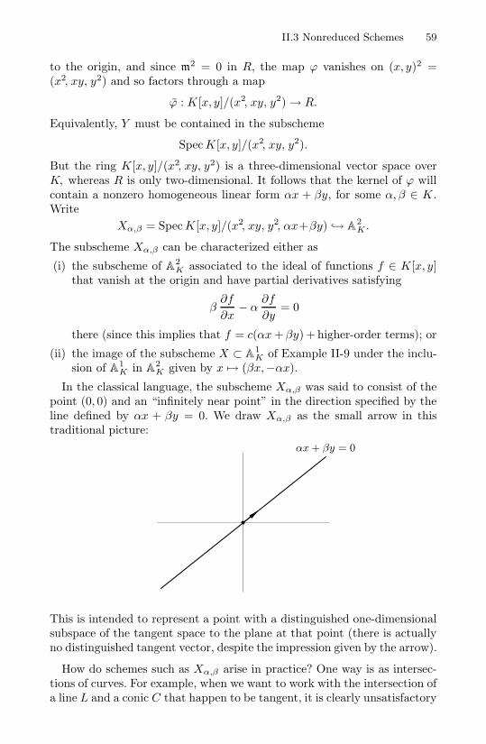
II.3 Nonreduced Schemes 59
to the origin, and since m2 = 0 in R, the map ϕ vanishes on (x, y)2 =(x2, xy, y2) and so factors through a map
ϕ : K[x, y]/(x2, xy, y2) → R.
Equivalently, Y must be contained in the subscheme
Spec K[x, y]/(x2, xy, y2).
But the ring K[x, y]/(x2, xy, y2) is a three-dimensional vector space overK, whereas R is only two-dimensional. It follows that the kernel of ϕ willcontain a nonzero homogeneous linear form αx + βy, for some α, β ∈ K.Write
Xα,β = Spec K[x, y]/(x2, xy, y2, αx+βy) → A2K .
The subscheme Xα,β can be characterized either as
(i) the subscheme of A2K associated to the ideal of functions f ∈ K[x, y]
that vanish at the origin and have partial derivatives satisfying
β∂f
∂x− α
∂f
∂y= 0
there (since this implies that f = c(αx + βy) + higher-order terms); or
(ii) the image of the subscheme X ⊂ A1K of Example II-9 under the inclu-
sion of A1K in A2
K given by x → (βx,−αx).
In the classical language, the subscheme Xα,β was said to consist of thepoint (0, 0) and an “infinitely near point” in the direction specified by theline defined by αx + βy = 0. We draw Xα,β as the small arrow in thistraditional picture:
αx + βy = 0
This is intended to represent a point with a distinguished one-dimensionalsubspace of the tangent space to the plane at that point (there is actuallyno distinguished tangent vector, despite the impression given by the arrow).
How do schemes such as Xα,β arise in practice? One way is as intersec-tions of curves. For example, when we want to work with the intersection ofa line L and a conic C that happen to be tangent, it is clearly unsatisfactory
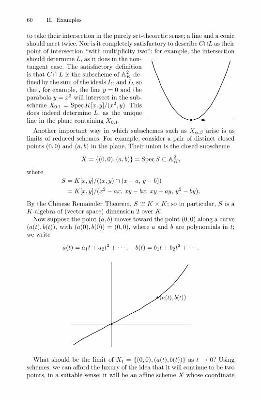
60 II. Examples
to take their intersection in the purely set-theoretic sense; a line and a conicshould meet twice. Nor is it completely satisfactory to describe C∩L as theirpoint of intersection “with multiplicity two”: for example, the intersectionshould determine L, as it does in the non-tangent case. The satisfactory definitionis that C ∩L is the subscheme of A2
K de-fined by the sum of the ideals IC and IL sothat, for example, the line y = 0 and theparabola y = x2 will intersect in the sub-scheme X0,1 = Spec K[x, y]/(x2, y). Thisdoes indeed determine L, as the uniqueline in the plane containing X0,1.
Another important way in which subschemes such as Xα,β arise is aslimits of reduced schemes. For example, consider a pair of distinct closedpoints (0, 0) and (a, b) in the plane. Their union is the closed subscheme
X = (0, 0), (a, b) = Spec S ⊂ A2K ,
whereS = K[x, y]/((x, y) ∩ (x − a, y − b))
= K[x, y]/(x2 − ax, xy − bx, xy − ay, y2 − by).
By the Chinese Remainder Theorem, S ∼= K × K; so in particular, S is aK-algebra of (vector space) dimension 2 over K.
Now suppose the point (a, b) moves toward the point (0, 0) along a curve(a(t), b(t)), with (a(0), b(0)) = (0, 0), where a and b are polynomials in t;we write
a(t) = a1t + a2t2 + · · · , b(t) = b1t + b2t
2 + · · · .
(a(t), b(t))
What should be the limit of Xt = (0, 0), (a(t), b(t)) as t → 0? Usingschemes, we can afford the luxury of the idea that it will continue to be twopoints, in a suitable sense: it will be an affine scheme X whose coordinate
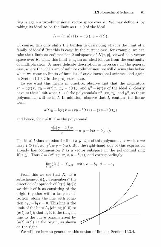
II.3 Nonreduced Schemes 61
ring is again a two-dimensional vector space over K. We may define X bytaking its ideal to be the limit as t → 0 of the ideal
It = (x, y) ∩ (x − a(t), y − b(t)).
Of course, this only shifts the burden to describing what is the limit of afamily of ideals! But this is easy: in the current case, for example, we cantake their limit as codimension-2 subspaces of K[x, y], viewed as a vectorspace over K. That this limit is again an ideal follows from the continuityof multiplication. A more delicate description is necessary in the generalcase, where the ideals are of infinite codimension; we will discuss this belowwhen we come to limits of families of one-dimensional schemes and againin Section III.3.2 in the projective case.
To see what this means in practice, observe first that the generatorsx2 − a(t)x, xy − b(t)x, xy − a(t)y, and y2 − b(t)y of the ideal It clearlyhave as their limit when t → 0 the polynomials x2, xy, xy, and y2, so thesepolynomials will be in I. In addition, observe that It contains the linearform
a(t)y − b(t)x = (xy−b(t)x) − (xy−a(t)y)
and hence, for t = 0, also the polynomial
a(t)y − b(t)xt
= a1y − b1x + t(. . .).
The ideal I thus contains the limit a1y−b1x of this polynomial as well; so wehave I ⊃ (x2, xy, y2, a1y − b1x). But the right-hand side of this expressionalready has codimension 2 as a vector subspace in the polynomial ringK[x, y]. Thus I = (x2, xy, y2, a1y − b1x), and correspondingly
limt→0
(Xt) = Xα,β with α = b1, β = −a1.
From this we see that X, as asubscheme of A2
K , “remembers” thedirection of approach of (a(t), b(t));we think of it as consisting of theorigin together with a tangent di-rection, along the line with equa-tion a1y− b1x = 0. This line is thelimit of the lines Lt joining (0, 0) to(a(t), b(t)); that is, it is the tangentline to the curve parametrized by(a(t), b(t)) at the origin, as shownon the right.
We will see how to generalize this notion of limit in Section II.3.4.

62 II. Examples
II.3.2 Multiple Points
The subschemes Xα,β of the preceding examples are called “double points”in the plane, the double referring to the vector space dimension of theircoordinate rings
R = K[x, y]/(x2, xy, y2, αx+βy) ∼= K[t]/(t2)
as K-modules. In general, if X = Spec R is an affine scheme and R is afinite-dimensional vector space over a field K, we define the degree of Xrelative to K, denoted degK(X) or simply deg(X), to be the dimension ofR as a K-vector space. (Where there is unlikely to be ambiguity about thefield K, we may suppress it in both the language and the notation.) In thissituation we call Spec R a finite K-scheme.
We next consider examples having degree 3 or more. A number of thingsare different here. To begin with, all double points over an algebraicallyclosed field K — that is, schemes of the form Spec R, where R is a localK-algebra of vector space dimension 2 — are isomorphic, since such an Rmust be isomorphic to K[x]/(x2). (Proof: Let m be the maximal ideal ofR. Then R/m ∼= K, since K has no finite-dimensional extension. Since Ris two-dimensional, m is one-dimensional. Also m2 = 0— for example, byNakayama’s Lemma — so the obvious map from K[x] onto R has x2 in thekernel and identifies R with K[x]/(x2) as required.) By contrast, this is nottrue of triple points: the schemes
Spec K[x]/(x3) and Spec K[x, y]/(x2, xy, y2)
are readily seen to be nonisomorphic. However, any triple point is isomor-phic to either of these, a fact whose proof we leave as the following exercise.
Exercise II-11. Suppose that K is algebraically closed, and let Z =Spec K[x1, . . . , xn]/I ⊂ An
K be any subscheme of dimension 0 and de-gree 3, supported at the origin. Show that Z is isomorphic either to X =Spec K[x]/(x3) or to
Y = Spec K[x, y]/(x2, xy, y2),
and X, Y are not isomorphic to each other.
In particular, any ring K[x1, . . . , xn]/I of vector space dimension 3 overK can be generated over K by two linear forms in the xi. In geometricterms, this says that any triple point in An
K is planar — that is, lies in alinear subspace A2
K ⊂ AnK . Inside A2
K both types of triple points can berealized as limits of triples of distinct points. The ones isomorphic to Xabove may be obtained from three points coming together in the plane alonga nonsingular curve, while those isomorphic to Y above arise when twopoints approach a third from different directions. The following exercisescontain examples of these phenomena.

II.3 Nonreduced Schemes 63
Exercise II-12. (i) Show that the subscheme of A2K given by the ideal
(y−x2, xy) arises as the limit of three points on the conic curve y = x2
and is isomorphic to X above, but is not contained in any line in A2K .
(i) (ii)
(ii) Show that subschemes of A2K isomorphic to Y above arise when two
points approach a third from different directions.
Exercise II-13. (For those familiar with the Grassmannian.) The exam-ples above may lead one to expect that the schemes isomorphic to X arelimits of those isomorphic to Y. In fact, just the opposite is the case, in thefollowing sense. Let H be the set of finite subschemes of degree 3 of A2
K
supported at the origin; H naturally parametrized by a closed subschemeof the Grassmannian of codimension-3 subspaces of the six-dimensionalvector space K[x, y]/(x, y)3. Show that H is a surface, with one point cor-responding to the unique subscheme Spec K[x, y]/(x2, xy, y2) isomorphic toY and the rest corresponding to subschemes isomorphic to X. Show thatthe scheme H is isomorphic to a two-dimensional cubic cone in P3
K , andthat the vertex is the one point corresponding to Y.
Exercise II-14. Let C be the subscheme of AnK given by the ideal
J = (x2 − x21, x3 − x3
1, . . .).
A closed point in C is of the form f(t) = (t, t2, t3, . . . , tn), for t ∈ K;that is, it has ideal (x1−t, x2−t2, . . .). Consider for t = 0 the three-pointsubscheme
Xt = f(0), f(t), f(2t) ⊂ C.
(a) Show that the limit scheme as t → 0 is
X0 = Spec K[x1, . . . , xn]/(x2 − x21, x1x2, x3, x4, . . . , xn)
and is isomorphic to the triple point Spec K[x]/(x3) above.
(b) Show, however, that X0 is not contained in the tangent line to C atthe origin. Rather, the smallest linear subspace of An
K in which X0 liesis the osculating 2-plane
x3 = x4 = · · · = xn = 0

64 II. Examples
to C (recall that this is by definition the limit of the planes spanned bythe tangent line and another point on C near the origin as the pointapproaches the origin), while the tangent line to C is the smallest linearsubspace of An
K containing the subscheme defined by the square of themaximal ideal in the coordinate ring of X0. Thus, in this sense, X0
“remembers” both the tangent line and the osculating 2-plane to C.
Exercise II-15. Consider for t = 0 the subschemes
Xt = (0, 0), (t, 0), (0, t) ⊂ A2K ,
each consisting of three distinct points in A2K .
(a) Show that the limit scheme as t → 0 is
X0 = Spec K[x, y]/(x2, xy, y2).
(b) Show that the restriction of a function f ∈ K[x, y] on A2K to X0 de-
termines and is determined by the values at the origin of f and itsfirst derivatives in every direction; thus we think of it as a first-orderinfinitesimal neighborhood of the point (0, 0).
(c) Show that X0 is contained in the union of any two distinct lines through(0, 0).
(d) Show that X0 is not contained in any nonsingular curve and thus, inparticular, is not the scheme-theoretic intersection of any two nonsin-gular curves in A2
K .
As we said, both types of triple point are contained in planes insideany affine space in which they are embedded. But the quadruple pointSpec K[x, y, z]/(x, y, z)2 is not, since its maximal ideal cannot be gener-ated by two elements. Other new phenomena occur for spatial multiplepoints— those not contained in the plane— and multiple points in higher-dimensional spaces. For example, not every point of degree 21 in 4-spacearises as a limit of sets of 21 distinct points, as the following exercise shows.(See also Iarrobino [1985].)
Exercise II-16. Consider zero-dimensional subschemes Γ ⊂ A4K of degree
21 such that
V (m3) ⊂ Γ ⊂ V (m4),
where m is the maximal ideal of the origin in A4K . Show that there is an
84-dimensional family of such subschemes, and conclude that a general oneis not a limit of a reduced scheme.
Exercise II-17. Classify up to isomorphism subschemes of A2K of dimen-
sion 0 and degrees 4 and 5 with support at the origin. Which are isomorphicas schemes over Spec K?

II.3 Nonreduced Schemes 65
Exercise II-18. A scheme Spec R supported at a point is called curvilin-ear if the maximal ideal of the (necessarily local) ring R is generated by oneelement; or, equivalently, if its Zariski tangent space has dimension zero orone. (The name comes from the fact that these are exactly the schemes thatcan be contained in a nonsingular curve.) Show that any two subschemesof A2
K having degree 2 and supported at a point can be transformed intoone another by a linear transformation of the plane, but that this is notpossible for curvilinear schemes of length 3. (Note, however, that any twocurvilinear subschemes of A2
K of the same degree can be carried into oneanother by an automorphism of A2
K .)
Exercise II-19. (For those with some familiarity with curves.) There areinfinitely many isomorphism types of degree-7 subschemes supported atthe origin in 3-space and infinitely many types of degree-8 subschemessupported at the origin in the plane.
As might be expected, the behavior of nonreduced schemes over non-algebraically closed fields is more complex. The following exercise gives anexample.
Exercise II-20. Classify all schemes of degree 2 and 3 over R supportedat the origin in A2
R . In particular, show that while any such scheme X whosecomplexification X ×SpecR Spec C is isomorphic to Spec C[x]/(x3) is itselfisomorphic to Spec R[x]/(x3), there are exactly two nonisomorphic schemesX whose complexification is isomorphic to Spec C[x, y]/(x2, xy, y2).
Degree and Multiplicity. Recall that on page 62 we defined the degreeof a finite affine K-scheme X = Spec R, where R is a finite-dimensionalvector space over some field K, as the dimension of R over K. When Kis algebraically closed, the degree of such a scheme X measures, in somesense, its nonreducedness. As the last exercise shows, however, this is nottrue in general: Spec C is reduced, but has degree 2 as a scheme over R.
There is an alternative concept, called the multiplicity, which measuresthe nonreducedness of X . Unlike the degree, which is a relative notiondependent on the specification of a base field K ⊂ R, the multiplicity isan invariant of X alone, and it is defined in a more general situation —we will define it here for any local ring R that has Krull dimension zero(equivalently, any local Artinian ring).
So let R be any zero-dimensional local ring, with maximal ideal m. It ispossible to choose ideals of R, say
R ⊃ m = I1 ⊃ I2 ⊃ · · · ⊃ Il−1 ⊃ Il = 0
such that each successive quotient Ij/Ij+1 is isomorphic to R/m as anR-module. (For example, we could start with the coarser filtration
R ⊃ m ⊃ m2 ⊃ · · · ⊃ 0
66 II. Examples
and refine it by choosing arbitrary subspaces of the R/m-vector spacesmj/mj+1.) Though such a filtration is not unique, the length l is indepen-dent of the filtration chosen; we define the multiplicity or length of the ringR and of the zero-dimensional scheme X to be the number l (see for ex-ample Eisenbud [1995, Section 2.4]). Notice that in the original situation,when R is an algebra over a field K, finite-dimensional as a vector spaceover K, the residue field R/m = κ is a finite extension of K and we havethe relation
degK(X) = [κ : K] mult(X).
For any zero-dimensional scheme X and point p ∈ X we define themultiplicity of X at p, denoted multp(X), to be the multiplicity of thelocal ring OX,p; if X is a finite K-scheme, the degree of X relative to K isgiven by
degK(X) =∑p∈X
[κ(p) : K] multp(X).
In Chapter III we will see how the notions of degree and multiplicity mayeach be extended to positive-dimensional schemes.
II.3.3 Embedded Points
We now consider some examples of nonreduced schemes of higher dimen-sion; for simplicity we will restrict ourselves to the case where the under-lying reduced scheme is a line. Even so, the variety of possible behaviorsincreases enormously; for example, we can have schemes that look likereduced schemes except at a point, or schemes that are everywhere nonre-duced. In this subsection, we consider the former type. By way of termi-nology, we will say that a scheme X = Spec K[x1 . . . , xn]/I ⊂ An
K has anembedded component if for some open subset U ⊂ An
K meeting X in a densesubset of X the closure of X ∩ U (as defined in Section I.2.1 above) doesnot equal X ; or if, equivalently, the primary decomposition of the ideal Icontains embedded primes (see the discussion of primary decompositionthat follows). If the embedded prime is maximal —equivalently, if U maybe taken to be the complement of a point— we talk about an embeddedpoint ; since the schemes X we will discuss below are all one-dimensional,this is all we will see.
The simplest example of a nonreduced scheme that is reduced except atone point is X = Spec K[x, y]/(y2, xy) ⊂ A2
K . The ideal I = (y2, xy) ⊂K[x, y] is the ideal of functions on the plane vanishing along the line y = 0and in addition vanishing to order 2 at the point (0, 0); in algebraic terms,this means that (y2, xy) = (y) ∩ (x, y)2. We can thus think of the schemeX as the line y = 0 with the proviso that a function f on X is defined byits restriction f(x, 0) to the line y = 0 together with the specification of itsnormal derivative at the point (0, 0) — that is, together with the number∂f/∂y(0, 0).

II.3 Nonreduced Schemes 67
It is convenient to realize X as the union of the line defined by y = 0with a nonreduced point— for example, the “first-order neighborhood ofthe origin” defined by the ideal (x2, xy, y2).
Such primary decompositions exist for any scheme: we briefly reviewthe background from algebra. For more details see, for example, Eisenbud[1995; Atiyah and Macdonald [1969], or, for perhaps the gentlest treatmentof all, Northcott [1953].
Primary Decomposition. Given any ideal I in a Noetherian ring R, wedefine the associated prime ideals of I to be the prime ideals p such that pis the annihilator of some element of R/I. These primes make up a finiteset.
An ideal q ⊂ p is called primary to p if p is the radical of q (the set ofelements having a power in q) and for any elements f, g in R with fg ∈ qbut f ∈ p we have g ∈ q; equivalently, q is p-primary if p is its radical andthe localization map R/q → Rp/qRp is a monomorphism.
Any ideal I may be expressed as the intersection of primary ideals. Sincethe intersection of ideals primary to a given prime ideal is again primaryto that prime, I can even be expressed as an intersection of ideals that areprimary to distinct prime ideals. If this is done in such a way that none ofthe primary ideals can be left out, the expression is called a primary decom-position of I. The primary ideals involved are called primary componentsof I.
The associated primes of I are exactly the radicals of the primary com-ponents. The primary component of I corresponding to a given associatedprime is not uniquely determined by I; it is, however, so determined if thecorresponding prime is minimal among the associated primes. Such primarycomponents are called isolated components.
Example II-21. Taking I = (y2, xy) as above, the decomposition
I = (y) ∩ (x, y)2
already given expresses I as an intersection of primary ideals (the first isprime, the second is primary to (x, y)).
Since neither (y) nor (x, y)2 can be omitted from this expression, it is aprimary decomposition and the associated schemes of X (as defined below)are precisely the line Xred and the reduced point at the origin. The primarycomponent associated to (x, y) in the decomposition is not unique; it couldhave been taken to be (x, y2), or (x+y, y2), or indeed any of an infinitenumber of other such ideals, as well as their intersection (x2, xy, y2), orfor that matter the ideal (xn, xy, y2) for any n ≥ 2. Of course, the primary

68 II. Examples
component (y) corresponding to (y) is unique, because Xred is not containedin any other associated scheme.
Despite this nonuniqueness, there is a well-defined length for the primarycomponent corresponding to a given associated prime p, which may becomputed, without choosing a primary decomposition, as the length of thelargest ideal of finite length in the ring Rp/IRp. Here the length of a moduleM is the maximal length l of a chain
M M1 M2 · · · Ml−1 Ml = 0
of submodules of M.
Exercise II-22. The length of the primary component of (xy, y2) at theorigin is 1.
It is easy to translate these matters into the geometry of schemes: anyaffine scheme X = Spec R, where R is Noetherian, is the union of “pri-mary” closed subschemes, called primary components, where a primaryaffine scheme is an affine scheme Y such that Yred is irreducible and suchthat, if f, g are functions on Y,
fg vanishes on Y butf does not vanish on Yred
=⇒ g vanishes on Y.
In such a primary decomposition of X, the components that are set-theore-tically maximal —called isolated components — are unique. The others—called embedded components, because their supports are contained in largercomponents— are not unique. Nonetheless, the decomposition does have atleast two nice uniqueness properties:
(1) The set of reduced subschemes associated to primary components ina minimal primary decomposition is unique; this is called the set ofassociated schemes to X.
(2) The “length” of the primary component associated to each of the asso-ciated schemes of X, called the multiplicity of that associated schemein X, is unique.
We may use our example X = Spec K[x, y]/(y2, xy) to illustrate thesenotions: we have already observed that X is the union of the line
Xred = Spec K[x, y]/(y)
and the multiple point
Y := Spec K[x, y]/(x2, xy, y2)
and we have seen that this gives a primary decomposition, the multiplicityof the embedded subscheme at the origin being 1.
As we observed, we can write X in many different ways as the unionof a line and a point: for example, for any α = 0, we have X = Y ∪ Z,

II.3 Nonreduced Schemes 69
where Z = Xred = Spec K[x, y]/(y) is the line and Y is, in the notation ofSection II.3.1, the subscheme X1,α:
Y = Spec K[x, y]/(x2, xy, y2, x+αy).
Choosing two such subschemes Y, Y ′ gives an example of closed subschemesY, Y ′ and Z in A2
K such that
Y ∪ Z = Y ′ ∪ Z and Y ∩ Z = Y ′ ∩ Z, but Y = Y ′.
In the example above, X can be described as the unique subscheme of A2K
consisting of the (reduced) x-axis plus an embedded point of multiplicity 1at the origin. But embedded points can carry geometric information, too.
Exercise II-23. Choose a linear embedding of A2K in A3
K , let P be theimage of A2
K , and let X ′ be the image of X. Show that X ′ determines Pas the unique plane in A3
K containing X ′.
It is also interesting to consider subschemes of A2K and A3
K supportedon a union of two given lines, with an embedded point of multiplicity 1 atthe intersection of the two lines. In the plane, if we take the two lines tobe the coordinate axes, such a scheme may be given as
X = Spec K[x, y]/(x2y, xy2).
Geometrically, this may be viewed as the union of the two lines defined byxy = 0 with the point Spec K[x, y]/(x3, x2y, xy2, y3). In 3-space, if we takethe lines to be (x = z = 0) and (y = z = 0), we can get such a schemeeither as
Y1 = Spec K[x, y, z]/(z, x2y, xy2)
or asY2 = Spec K[x, y, z]/(z2, xz, yz, xy).
Y1 is the image of the scheme X above under the embedding of A2K into
A3K as the plane z = 0, whereas Y2 is the union of the two lines with the
subscheme of A3K defined by the square of the maximal ideal of the origin
in A3K .
Exercise II-24. (a) Show that Y1 ∼= Y2.
(b) Show that Y1∼= X is, up to isomorphism, the unique example contained
in a plane of two lines meeting in a point and having an embedded pointof multiplicity 1 at that intersection point.
(c) Show that Y2 is, up to isomorphism, the unique example contained in3-space but not in any plane of two lines meeting in a point and havingan embedded point of multiplicity 1 at that intersection point.
One justification for the idea that the multiplicity of the embedded pointat the origin in our scheme X = Spec K[x, y]/(xy, y2) is 1 is that X is the

70 II. Examples
limit as t → 0 of the family of subschemes
Xred ∪ Yt ,
where Yt is the scheme consisting of one reduced point
Spec K[x, y]/(x, y−t) ⊂ A2K .
This is plausible since the ideal
(x, y−t) ∩ (y) = (xy, y2−ty)
of Xred ∪ Yt naturally seems to approach (xy, y2) at t → 0. However, thenotion of limit that we introduced earlier is not quite strong enough to dealwith this example, since the ideal (x, y−t)∩ (y) of Xred ∪Yt is not of finitecodimension. In the next section we will rectify this, describing the generalcontext for taking limits of schemes.
II.3.4 Flat Families of Schemes
The notion of a family of schemes is extremely general: we define a family ofschemes to be simply a morphism π : X → B of schemes! The individualschemes in the family are the fibers of π over points of B. This notionincludes all others that one can think of, such as a scheme defined by“equations with parameters”, B being the space on which the parametersvary.
However, the notion of a family as an arbitrary morphism π : X → B isso general as to be virtually useless, because the fibers of the family mayhave nothing in common. For example, given such a family and a closedpoint b ∈ B, one could make a new family by replacing X by the disjointunion of X−π−1b and some other scheme Y, sending all of Y to b. Thus wemust add some condition if we wish to have families of schemes that varycontinuously, in some reasonable sense. What “reasonable” should meanis not obvious. It seems natural at least to ask that it include the motherof all continuously varying families, the family of projective plane curvesof a given degree (see Section III.2.8). Other examples are the familiesof schemes defined by families of ideals of constant finite codimension ina polynomial ring, as we considered in the context of limits of multiplepoints.
In many geometric theories one gets the right notion of a continuouslyvarying family by demanding some local triviality of the family; that is,locally, in some suitable sense, the family should look like the projection ofa direct product to one factor. This is wrong for us on two counts. First,if we do this naively for schemes, interpreting locally as meaning locallyin the Zariski topology, we get a notion that is far too restrictive to be ofmuch use. A more sophisticated approach would be to demand this localtriviality analytically; that is, to demand that if x ∈ X and b = π(x),then the completion of the local ring OX,x should look like a power series

II.3 Nonreduced Schemes 71
ring over the completion of the local ring OB,b. This notion is quite useful(it is called smoothness), but it excludes, for example, the family of planecurves of a given degree, since a smooth family can’t have singular fibers.Smoothness also excludes the families treated in the previous section, inwhich a disjoint union of distinct points approaches a multiple point; at themultiple point, the criterion is not met. Thus we must look for somethingmore general.
The best current candidate for such a general notion is that of flatness.In order to motivate this definition, we consider first the more intuitivenotion of limits.
Limits. The starting point for understanding the geometric content offlatness is the notion of the limit of a one-parameter family of schemes.
To set this up, we start with something fairly concrete: A family ofclosed subschemes of a given scheme A over a base B is a closed subschemeX ⊂ B × A, together with the restriction to X of the projection mapB×A → B; the fibers of X over b ∈ B are then naturally closed subschemesof the fibers Ab of B × A over B.
Let B be a nonsingular, one-dimensional scheme— typically, we thinkof Spec R, where R = K[t], K[t](t) or K[[t]], but any Dedekind domain(including Z or Z(p)) will do. Let 0 ∈ B be any closed point, and writeB∗ = B \ 0 for the complement of 0 in B. Let An
B and AnB∗ be as usual
affine n-space over B and B∗ respectively.We consider a closed subscheme X ∗ ⊂ An
B∗ = AnZ × B∗, which we
view as a family of closed affine schemes parametrized by B∗ — that is, forany point b ∈ B∗ we let Xb = π−1(b) be the fiber of the projection mapπ : X ∗ → An
B∗ → B∗, and consider these schemes Xb as the members ofa family. (In case B = Spec R with R = K[t] or K[t](t) we can think ofX ∗ as a “family of subschemes of An
K varying with parameter t”.) We askthe basic question: what is the limit of the schemes Xb as b approaches thepoint 0?
X ∗
B∗
AnB

72 II. Examples
The answer— the only possible answer— is simple enough: since thelimit of the schemes Xb in any reasonable sense must fit into a familywith them, we take X ⊂ An
B to be the closure X ∗ of X ∗ in AnB, and take
the limit limb→0 Xb of the schemes Xb to be the fiber X0 of X over thepoint 0 ∈ B.
To make this more concrete, if B = Spec R is affine and t ∈ R a generatorof the maximal ideal m ⊂ R corresponding to the point 0 ∈ B (so that B∗ =Spec R[t−1]), and I(X ∗) ⊂ R[t−1][x1, . . . , xn] is the ideal of X ∗ ⊂ An
B∗ ,then the ideal of the subscheme X ⊂ An
B is the intersection
I(X ) = I(X ∗) ∩ R[x1, . . . , xn].
To be even more concrete, if we take B = Spec K[t], the limiting schemeX0 ⊂ An
K is cut out by the limits of polynomials vanishing on the schemesXt —in other words, if we view the ideals I(Xt) ⊂ K[x1, . . . , xn] as linearsubspaces of the K-vector space K[x1, . . . , xn] and let V ⊂ K[x1, . . . , xn]be the limiting position of the planes I(Xt), the ideal I(X0) is generatedby V. Thus this definition of limit generalizes the naive notion used inSection II.3.1.
For example, take B = Spec K[t] and B∗ = B \0 = Spec K[t, t−1], andlet Xt be the subscheme of A1
K consisting of the two points with coordinatest and −t— that is, take X ∗ = V (x2 − t2) ⊂ Spec K[t, t−1][x] = A1
B∗ .Then the closure X of X ∗ in An
B is given again as X = V (x2 − t2) ⊂Spec K[t][x] = A1
B, and the fiber X0 of X over the point 0 ∈ B is simplythe double point X0 = V (x2) ⊂ A1
K .The notion of the limit of a family of schemes X ∗ ⊂ An
B∗ depends verymuch on the embedding in An
B∗ , not just on the abstract family X ∗ → B∗.Thus, in the preceding example, the schemes Y ∗ = V (x2 − 1) and Z ∗ =V (x2−t−2) ⊂ Spec K[t, t−1][x] = A1
B∗ are isomorphic as B∗-schemes to thescheme X ∗, but the limit of Y ∗ is the two reduced points V (x2−1) ⊂ A1
K
and that of Z ∗ is the empty set.
Examples. The examples of limits we have encountered up to now have allinvolved limits of zero-dimensional schemes. Here are a couple of examplesinvolving positive-dimensional ones. They are instructive also because theyillustrate how embedded points arise naturally in limits of varieties.
The first example is that of three lines through the origin in affine 3-space A3
K over a field K. We take the three coordinate axes, rotate onedown until it lies in the plane of the other two, and ask what is the limitof this family. Specifically, in A3
K = Spec K[x, y, z] we let L = V (y, z) bethe x-axis and M = V (x, z) the y-axis, and let Nt be the line
Nt = V (x−y, z−tx).
For t = 0 we let Xt = L ∪ M ∪ Nt. The curves Xtt=0 form a familyX ∗ ⊂ A3
B∗ over the base B∗ = Spec K[t, t−1], and we ask for the limit X0
of this family.

II.3 Nonreduced Schemes 73
This is straightforward to calculate, though the answer may initially besurprising. The ideal of the union of the three coordinate axes is (xy, xz, yz),so the ideal of the scheme Xt for t = 0 is generated simply by products oflinear forms:
I(Xt) = (Q1, Q2, Q3),
whereQ1 = z (z − tx),Q2 = z (z − ty),Q3 = (z − tx)(z − ty).
When we let t go to zero, we see that the ideal of the limiting schemecontains z2, the common limit of Q1, Q2 and Q3. In addition, for t = 0the ideal I(Xt) contains Q1 −Q3 = tyz − t2xy and Q2 − Q3 = txz − t2xy.Thus, for t = 0 the ideal contains
Q1 − Q3
t= yz − txy and
Q2 − Q3
t= xz − txy,
and hence the ideal of the limiting scheme X0 contains xz and yz. Finally,the ideal of Xt contains
xQ1 − Q3
t− y
Q2 − Q3
t= txy (x − y),
and hence the ideal of the limiting scheme contains xy (x − y). Thus wehave
I(X0) ⊃(xz, yz, z2, xy (x−y)
)and we claim that in fact this is an equality. We will establish this in amoment, but before we do we should point out the striking fact about this:the limit scheme X0 of the family of schemes Xt = L∪M ∪Ntt=0 is notsimply the union L ∪ M ∪ N0. In fact, the ideal of the union is
I(L ∪ M ∪ N0) =(z, xy (x−y)
),
so thatI(X0) = I(L ∪ M ∪ N0) ∩ (x, y, z)2.
In other words, the limit scheme X0 has an embedded point at the origin.In fact, it’s not hard to see this directly, which in turn allows us to prove
the equality I(X0) = (xz, yz, z2, xy (x−y)): the schemes Xt all have three-dimensional Zariski tangent space at the origin (0, 0, 0) ∈ A3
K , so X0 mustas well, because if X ⊂ An
B is any closed subscheme and σ : B → X anysection of X → B, the dimension of the Zariski tangent space Tσ(b)X isan upper-semicontinuous function of b ∈ B. This in turn implies that
I(X0) ⊂ I(L ∪ M ∪ N0) ∩ (x, y, z)2 =(xz, yz, z2, xy (x−y)
),
from which equality follows.

74 II. Examples
A similar example is the limit of the scheme consisting of two disjointlines in A3
K as the lines move to meet in a single point. As the followingexercise shows, their limit actually has an embedded point at the point ofintersection:
Exercise II-25. Let Lt be the line in A3K defined by the ideal (y, z−t)
and M be the line defined by (x, z); for t = 0 let Xt be their union. Showthat the limit of Xt as t → 0 is the scheme
X0 = Spec K[x, y, z]/(z2, xz, yz, xy).
y = z − t = 0 x = z = 0
Xt
y = z = 0
x = z = 0
X0
The following exercise shows that the appearance of the embedded pointin the limit is no accident:
Exercise II-26. (a) Show that there does not exist a family of lines Lt ⊂A3
K disjoint from M = V (x, z) parametrized by B∗ = Spec K[t, t−1]such that the limit of M ∪ Lt as t → 0 is the reduced scheme
X = Spec K[x, y, z]/(z, xy).
(b) Similarly, show that there does not exist a family of lines Lt ⊂ A3K
parametrized by B∗ = Spec K[t, t−1] such that the limit of M ∪ Lt ast → 0 is the scheme
X = Spec K[x, y, z]/(z, x2y, xy2).
Note that in these two examples, as well as those analyzed earlier, thelimit of a union of schemes properly contains the union of their limits. Wewill return to this in Chapter V.
Taking the limit of a one-parameter family of subschemes of a givenscheme is a fundamental operation in algebraic geometry. In the examplesoccurring throughout the remainder of this book, we will calculate theideals of such limits by ad-hoc methods, as we’ve done here. But thereis a general algorithm, best carried out by machines, for performing thiscomputation. For example, suppose that the base B = Spec K[t], and wehave an ideal I ⊂ K[t][x1, . . . , xn] such that for λ = 0 the scheme Xλ ⊂An
K is defined by the ideal
Iλ = (I, t−λ)/(t−λ) ⊂ K[t][x1, . . . , xn]/(t − λ) ∼= K[x1, . . . , xn].

II.3 Nonreduced Schemes 75
Then we define an ideal J ⊂ K[t][x1, . . . , xn] by setting
J =⋃k
(I : tk);
that is, J is the ideal of polynomials f(t, x1, . . . , xn) such that tkf ∈ Ifor some k. This can be computed using Grobner bases; see Eisenbud [1995,Chapter XV].
Flatness. The preceding discussion suffices to describe the notion of acontinuously varying family of subschemes of a fixed scheme A (such asaffine or projective space) over a nonsingular one-dimensional base: we saysuch a family X ⊂ B × A is continuous if each fiber is the limit of nearbyones. This notion is still too restrictive, however: it does not suffice, forexample, if the base B is nonreduced, a case that turns out to be of greatutility. To extend the notion to the most general setting, Serre introducedthe following notion:
Definition II-27. A module M over a ring R is flat if for every monomor-phism of R-modules A → B the induced map M ⊗R A → M ⊗R B is againa monomorphism.
In particular, any free module is flat; and thus if R is a field, every moduleis flat. It is not hard to show that if R is a Dedekind domain, then M is flatif and only if M is torsion-free. We next make the corresponding geometricdefinition:
Definition II-28. A family π : X → B of schemes is flat if for every pointx ∈ X the local ring OX,x, regarded as an OB,π(x)-module via the map π#,is flat.
This notion is general enough to include the families of plane curves ofgiven degree but restrictive enough so that the varieties in a flat family havea lot in common. It is really quite satisfactory, except for the fact that—initially, at least — it does not seem to be a very “geometric” property. Infact, however, it is the most natural— indeed, the only possible— extensionof the naive notion of limits introduced above! We will establish this fact,and then go on to consider other properties of the notion of flatness; seeEisenbud [1995; Matsumura [1986; Hartshorne [1977] for good technicaldiscussions.
To begin with, flatness expresses the quality we desire in the cases wehave already considered:
Proposition II-29. Let B = Spec R be a nonsingular, one-dimensionalaffine scheme, 0 ∈ B a closed point and B∗ = B \0. Let X ⊂ An
B be anyclosed subscheme, and π : X → B the projection. The following conditionsare equivalent:
(1) π is flat over 0.

76 II. Examples
(2) The fiber X0 = π−1(0) is the limit of the fibers Xb = π−1(b) as b → 0.
(3) No irreducible component or embedded component of X is supportedon X0.
Proof. We start with the equivalence of (2) and (3). Set X ∗ = π−1(B∗) ⊂X . Since X ⊂ An
B is closed, it contains the closure of X ∗; so the fiberX0 = π−1(0) contains the limit of the fibers Xb = π−1(b) as b → 0, and tosay that X0 = limb→0 Xb is simply to say that we have equality: X = X ∗.Conversely, X0 properly contains the limit of the Xb if and only if X ∗ X ,that is, the expression
X = X ∗ ∪ X0
as a union of closed subschemes is nontrivial. Thus (2) and (3) are equiva-lent.
To see that (1) is equivalent to (3), simply observe that OX ,x, regardedas an OB,0-module, is flat for all x ∈ X0 if and only if OX (X ) is torsion-free as an R-module (see Bourbaki [1972, I.2.4, Proposition 3.ii]; becauseall these rings R are principal ideal domains, this also follows easily fromMatsumura [1986, Theorem 7.6 and its converse on p. 50] or Eisenbud[1995, Corollary 6.3]).
How general is this interpretation of flatness? To begin with, since thecondition of flatness is local in the domain of a morphism π : X → B,the assumption that X and B are affine is really no restriction at all. Ifwe assume that X is of finite type over B, a mild extra finiteness condi-tion described in Section III.1.1, we can further reduce to the case whereX is a closed subscheme of An
B and π is the restriction to X of the pro-jection An
B → B. All these are minor hypotheses. The serious restrictionin applying the preceding result is that we take B to be nonsingular andone-dimensional. We can, however, broaden this substantially with the fol-lowing lemma, which characterizes flat families of finite type over a reducedbase.
Lemma II-30. Let K be a field, B a reduced K-scheme, b ∈ B a closedpoint and X ⊂ An
B a closed subscheme. X is flat over b if and only if forany nonsingular, one-dimensional K-scheme B′, any closed point 0 ∈ B′
and any morphism ϕ : B′ → B carrying 0 to b, the fiber Xb is the limit ofthe fibers Xϕ(b′) as b′ approaches 0 —that is, for any ϕ : B′ → B carrying0 to b, the pullback family
X ′ = X ×B B′ ⊂ AnB′ → B′
is flat over 0.
Proof. Since Xϕ(b′) = X ′b′ , Proposition II-29 asserts the equivalence of the
limit condition Xb = limb′→0 Xϕ(b′) with the flatness of X ′ over B′. Thatsaid, one direction is clear: in general, if X → B is flat and B′ → B is any

II.3 Nonreduced Schemes 77
morphism, the fiber product X ×B B′ → B′ is flat; see Matsumura [1986,Chapter 2, Section 3]. For the other direction, which is much harder, seeRaynaud and Gruson [1971, Cor. 4.2.10].
When the conditions of Lemma II-30 are met, we will call the fiber Xb
the flat limit of the nearby fibers of X over B.
A word of warning: while for B one-dimensional and 0 ∈ B a nonsin-gular point there exists a unique flat limit of a given family X ⊂ An
B∗
over B∗ = B \ 0, two-parameter families may not admit any flat lim-its at all. Consider for example the degree-2 subschemes of A2
K discussedearlier. We take as our base the scheme B = Spec K[s, t] = A2
K , withthe origin as our special point 0 ∈ B. For (s, t) = (0, 0) ∈ B, we letXs,t ⊂ Spec K[x, y] = A2
K be the subscheme consisting of the union of thepoints (x, y) and (x−s, y−t) ∈ A2
K . These subschemes form a family X ∗
over B∗ = B \ 0, defined by
X ∗ = V(x(x−s), x(y− t), y (x−s), y (y− t)
) ⊂ A2B∗ .
But we have seen that the limits of the schemes Xs,t as (s, t) approaches theorigin along lines of different slope are different double points: all supportedat the origin, of course, but with different tangent lines. The fiber X0 of theclosure X = X ∗ ⊂ A2
B of X ∗ in A2B over the origin 0 ∈ B must therefore
contain the union of these double points, that is, it must contain the “fatpoint” V (x2, xy, y2) ⊂ A2
K . It follows that the closure must be simply thesubscheme
X = V(x(x−s), x(y− t), y (x−s), y (y− t)
) ⊂ A2B,
whose fiber over the origin is V (x2, xy, y2). We see in particular that noclosed subscheme of A2
B containing X ∗ as an open subscheme can be flatover 0 ∈ B.
The morphism X → B here is the same as the morphism X → Y ofExercise I-43(b): the scheme X is the union of two planes in affine four-space A4
K meeting at a point, with the projection X → B an isomorphismon each plane. In particular, the failure of the family X ∗ ⊂ A2
B∗ to have aflat limit is very much a function of the embedding in A2
B∗ : outside of theorigin in A2
B, we could include X ∗ in the disjoint union A2B
∐A2
B of twocopies of A2
B to obtain a surjective morphism ν : X → B with ν−1(B∗) ∼=X ∗ as B∗-schemes. Thus the failure of this family to have a flat limit mightbe ascribed to our perversity in choosing a bad embedding of X ∗ in A2
B .The following exercise gives another classic example of a nonflat family,and one that moreover has no flat limit, irrespective of the embedding.
Exercise II-31. Consider the cone B = V (su − t2) ⊂ Spec K[s, t, u] =A3
K . Let 0 = (s, t, u) ∈ B be the origin, and let B∗ = B \ 0 as usual.Set X = Spec K[x, y] = A2
K , and let ϕ : X → B be the map dual to theinclusion of rings
ϕ# : K[s, t, u]/(su − t2) −→ K[x, y]

78 II. Examples
sending s to x2, t to xy, and u to y2. (Equivalently, B is simply the quotientof X = A2
K by the involution (x, y) → (−x,−y), and ϕ the quotient map.)Let X ∗ be the inverse image ϕ−1(B∗) ⊂ X . Show that X → B is not flatover 0.
In fact, the family X ∗ → B∗ has no flat limit, in the sense that thereis no scheme Y and surjection ν : Y → B such that ν−1(B∗) ∼= X ∗
as B∗-schemes. Nor is this really pathological: in Section IV.3.2 we’ll seeexamples of naturally occurring families that don’t admit flat limits.
Proposition II-29 and Lemma II-30 together give us a geometric inter-pretation of the flatness of a morphism ϕ : X → B, at least in casewhere X is of finite type over a base B that is reduced and over a field:it says that ϕ is flat at p if, under any embedding of a neighborhood ofp ∈ X in affine space An
B, the fiber X0 = ϕ−1(0) over 0 = ϕ(p) ∈ B is(an open subset of) the limit of the fibers Xb as b ∈ B approaches 0 alongany one-parameter family. The wonderful thing about the definition of flat-ness in general is that it takes this basic notion and extends it, in a verynatural way, to arbitrary morphisms! This is particularly remarkable (anduseful) in case the base space B is a nonreduced scheme. If, for example,B = Spec K[ε]/(ε2), it makes no sense to talk about the “fibers of X → Bover nearby points”; B has only one point. Nonetheless (as we will see ex-plicitly in Chapter VI) it does make sense to talk about families X → B ofschemes parametrized by B “varying continuously”; flatness exactly cap-tures this property. (Even in case the base B has one-dimensional Zariskitangent space, as in the example B = Spec K[ε]/(ε2), we can’t just use thecriterion that no component of X , irreducible or embedded, is supportedon the inverse image of the reduced point Bred: for example, the morphismSpec K[x, y]/(x2, xy, y2) → Spec K[ε]/(ε2) dual to the ring homomorphismε → x is not flat.)
In general, if B = Spec R is the spectrum of a local Artinian ring Rwith maximal ideal m, 0 = V (m) = Bred ⊂ B its unique point, a flatmorphism ϕ : X → B is called an “infinitesimal deformation” of the fiberX0 = ϕ−1(0). Such things played an important role in the algebraizationof the theory of curves on surfaces — see, for example, Mumford [1966] andthe discussion in Section VI.2.3.
To conclude this section, we mention (without proof) two facts aboutflatness, both of which will reaffirm that flatness is indeed the correct cri-terion for a family X → B of schemes to be “varying continuously”. Thefirst is one we mentioned at the outset: we would like families of hypersur-faces to be flat. Explicitly, if
f(x1, . . . , xn) =∑
aIxI
is a polynomial in n variables whose coefficients aI are regular functionson a scheme B, then the corresponding subscheme V (f) ⊂ An
B should beflat over B, at least away from the common zero locus V (aI) ⊂ B of the

II.3 Nonreduced Schemes 79
coefficients. In fact, more is true: the same holds for families of completeintersections X = V (f1, . . . , fc) ⊂ An
B. We state this as follows:
Proposition II-32. Let R be a local ring with maximal ideal m, B =Spec R, 0 = [m] ∈ B the unique closed point of B and κ = κ(0) = R/m theresidue field. Let f1, . . . , fc ∈ R[x1, . . . , xn] be polynomials with coefficientsin R, and
X = V (f1, . . . , fc) ⊂ Spec R[x1, . . . , xn] = AnB .
If the fiber X0 = π−1(0) of the projection π : X → B over 0 has codimen-sion c in An
κ, then X → B is flat.
More generally, we have the following criterion for flatness, which is ex-tremely useful in practice.
Exercise II-33. (a) Prove that a module M over the ring R = K[t](t) isflat if and only if t is a nonzerodivisor on M, that is, if and only if Mis torsion-free.
(b) Let A = R[x1, . . . , xn] be a polynomial ring over R = K[t](t), and letM be an A-module with free presentation
F1ϕ−→ F0 −→ M −→ 0.
Consider the module M := M/Mt over the factor ring A := A/tA, andlet
F1ϕ−→ F0 −→ M −→ 0
be the corresponding presentation. Show that M is flat over R if andonly if every second syzygy of M over A can be lifted to a secondsyzygy over A in the sense that every element of the kernel of ϕ comesfrom an element of the kernel of ϕ. (Something similar is true for anylocal base ring R with maximal ideal m if M is finitely generated overA; this is a form of the “local criterion of flatness”— see, for example,Eisenbud [1995, Section 6.4] or Matsumura [1986, p. 174].
A second thing that makes flatness a good notion is the generic flatnesstheorem, due to Grothendieck (see for example Eisenbud [1995, Section14.2]. This says that if one has any reasonable family of schemes X → Bover a reduced base, then there is an open dense subset U of B such thatthe restricted family π−1U → U is flat (here “reasonable” includes, forexample, any family of subschemes of a fixed affine or projective space).In some sense this vindicates our choice of flatness as the analogue of thenotion of bundle in topology: it is analogous to the observation that iff : M → N is a differentiable map of compact C∞ manifolds, then thereis a dense collection of open subsets U of the target space N such that therestriction of f to each f−1(U) is a fiber bundle. In any event, the genericflatness theorem certainly assures us that flat families are ubiquitous inalgebraic geometry.

80 II. Examples
This concludes our initial discussion of flatness. We will see other ge-ometric interpretations of flatness when we discuss families of projectiveschemes in Chapter IV.
II.3.5 Multiple Lines
We now consider a nonreduced affine scheme X supported on a line andnot having embedded components. We will assume that the multiplicityof the line (in the sense of the primary decomposition) is 2, and we willanalyze the possibilities.
It is very easy to write down a first example: the scheme
X = Spec K[x, y]/(y2) ⊂ A2K
obviously has the desired properties. It’s pretty clear that there are no moreexamples supported on the line y = 0 in A2
K , but we can construct many inA3
K . A subscheme X of the sort we want will meet a general plane in A3K
passing through a point of the reduced line in a double point contained inthat plane. We already know that any double point may be thought of as apoint plus a tangent vector at that point, and this suggests that we obtainX by choosing a normal direction at each point of the line. For example,take L := Xred to be the line x = y = 0, with coordinate z. Now, choose apair of polynomials p and q in z without common zeros, and at each point(0, 0, z0) ∈ L take the normal direction to be the one with slope p(z0)/q(z0)in the normal plane z = z0. It is easy to see that the union over all z of thedouble points in the given directions will be contained in the scheme Xp,q
defined by taking
Ip,q = (x2, xy, y2, p(z)x−q(z)y)
andXp,q = Spec K[x, y, z]/Ip,q
The simplest nonplanar example would be one where the chosen normaldirections twist just once around L— for example, the one given by theideal
IΓ = (x2, xy, y2, zy−x).
z

II.4 Arithmetic Schemes 81
Exercise II-34. If p, q are relatively prime polynomials, then the ideal
(x, y)/Ip,q
in the ringK[x, y, z]/Ip,q
is torsion-free of rank 1 as a K[z]-module; thus Xp,q is primary, with(Xp,q)red the line Spec K[x, y, z]/(x, y), and Xp,q has multiplicity 2.
At first sight it looks as though these examples will possess many in-teresting invariants and thus, in particular, be distinct, but this is not so:we can “untwist” any of the schemes Xp,q by an automorphism of A3
K togive an isomorphism of it with the planar double line SpecK[y, z]/(y2).To do this, note that since p and q have no common zeros, we may write1 = aq + bp for some polynomials a, b ∈ K[z]; thus the matrix(
a bp −q
)
has unit determinant, so the map A3K → A3
K given by
(x, y, z) → (x′, y′, z), with x′ := p(z)x − q(z)y, y′ := a(z)x + b(z)y,
is invertible. Again because the matrix is invertible, we have
(x, y) = (x′, y′) and (x2, xy, y2) = (x′2, x′y′, y′2)
so the ideal of Xp,q is (x, x2, xy, y2) = (x, y2), as required.More generally, it turns out that there is up to isomorphism only one
affine double line, in the following sense:
Exercise II-35. Prove that if A is a Noetherian K-algebra such thatX = Spec A has no embedded components, has multiplicity 2, and sat-isfies Xred
∼= A1K , then X is isomorphic to Spec K[x, y]/(y2).
We will see in the next chapter that this situation contrasts with the onein projective space: there are many nonisomorphic projective double lines.
II.4 Arithmetic Schemes
Our last collection of examples will be spectra of rings that are finitelygenerated and reduced but that do not contain any field at all. In general,the spectra of rings finitely generated over Z are called arithmetic schemes;they arise primarily in the context of number theory, although by no meansall schemes of number-theoretic interest are of this type. In these exampleswe will see some hint of the amazing unification that schemes allow betweenthe arithmetic and the geometric points of view.

82 II. Examples
II.4.1 Spec Z
We start with the most obvious example, the scheme Spec Z itself. Theprime ideals of Z are, of course, the ideals (p), for p ∈ Z a prime number,and the ideal (0); the former correspond to closed points of Spec Z, withresidue field Fp, while the latter is a “generic” point, whose closure is allof Spec Z and whose residue field is Q. The picture is this:
(0)(2) (3) (5) (7) (11)
This bears a formal resemblance to an affine line A1K over a field; indeed,
this similarity is just the beginning of a long sequence of analogies, and itis well to bear it in mind while looking at the following examples. However,the analogy also has its limits: while Spec Z behaves much like A1
K , forexample, it is not an open dense subscheme of any scheme analogous toP1
K .
II.4.2 Spec of the Ring of Integers in a Number Field
Secondly, consider a scheme of the form Spec A, where A ⊂ K is the ringof integers in a number field K; we will analyze the example K = Q[
√3]
and A = Z[√
3]. As in the case of Spec Z, there are just two types ofpoints: closed points corresponding to nonzero prime ideals in A, havingfinite residue fields, and a generic point corresponding to (0) with residuefield K. What makes this example interesting is the map Spec A → Spec Zinduced by the inclusion of Z in A. Consider, for example, the fiber overa point [(p)] ∈ Spec Z. This is just the set of primes in A containing theideal pA ⊂ A, and it may behave in any one of three ways (a good basicreference for the unexplained material here is Serre [1979]):
(1) If p divides the discriminant 12 of K over Q — that is, for p = 2 or 3 —the ideal (p) is the square of an ideal in A: we have
2A = (1 +√
3)2
and, of course,3A = (
√3)2.
The residue fields at the points (1 +√
3) and (√
3) ∈ Spec A are thefields F2 and F3, respectively.
(2) Otherwise, if 3 is a square mod p, the prime (p) will factor into aproduct of distinct primes: for example
11A = (4 + 3√
3)(4 − 3√
3)
and13A = (4 +
√3)(4 −
√3).

II.4 Arithmetic Schemes 83
The residue fields at these points will again be the prime fields, in thiscase F11 and F13, respectively.
(3) Finally, if p > 3 and 3 is not a square mod p— for example, when p = 5or 7— the ideal pA is still prime and corresponds to a single point inSpec A. In these eases, the residue field is the quadratic extension ofFp —for instance, F25 and F49 in the two examples.
In general, as in this example, if K is a quadratic number field, and Ais the ring of algebraic integers in K, then the inclusion Z ⊂ A induces amap of schemes ψ : Spec A → Spec Z whose fiber over each closed point(p) ∈ Spec Z is one of the following:
(1) A single, nonreduced point, with coordinate ring isomorphic to A/p2,whose underlying reduced point p has residue field Fp, if p ramifies inA— that is, if pA is the square of a prime ideal p of A.
(2) The disjoint union of two reduced points, p and p′, with residue fieldsA/p = A/p′ = Fp, if pA is a product of two distinct prime ideals of A.
(3) A single reduced point p, with residue field A/p of degree 2 over Fp, ifp remains prime in A.
In every case the coordinate ring of the fiber has dimension 2 as an Fp-algebra. That is because A is a free Z-module of rank 2. Of interest hereis the analogy between the map Spec A → Spec Z and a branched cover ofRiemann surfaces (or, more generally, of one-dimensional schemes over analgebraically closed field such as C). Essentially, we may think of Spec A asa two-sheeted cover of Spec Z, with branching over the “ramified” primes,just as, for example, Spec C[z] is a double cover of Spec C[z2] branchedover the origin. The one apparent difference is that over some points (p) ∈Spec Z other than ramification points we may have, instead of two distinctpoints with multiplicity 1, one point with multiplicity 1 but with a residuefield that is a quadratic extension of the residue field Fp at (p). These aredenoted by uniform gray dots in the picture:
(0)(2) (3) (5) (7) (11) (13)(5) (7)
(1+√
3) (√
3)(5) (7)
(4+3√
3)
(4−3√
3)
(4+√
3)
(4−√3)
A more inclusive analogy would be with a finite map between one-dimensional schemes over a non-algebraically closed field. Consider, forexample, the map
Spec R[x][y]/(y2 − x) → A1R = Spec R[x]
Looking just at points of A1R = Spec R[x] with residue field R — that is,
points of the form (x−λ) with λ real — we have ramification over the point

84 II. Examples
(x), and for λ = 0 the inverse image of (x−λ) is either two distinct pointswith residue field R (if λ > 0) or one point with residue field C (if λ < 0).
We may continue this analogy a little further by looking at schemes ofthe form Spec B, where B ⊂ A ⊂ K is an order in a number field—that is, a subring of the ring of integers in K having quotient field K. Forexample, let A = Z[
√3] and consider the ring B = Z[11
√3] and the asso-
ciated scheme Spec B. The map Spec A → Spec Z described above factorsthrough Spec B, and indeed the map Spec A → Spec B is an isomorphismexcept that the two points (4 + 3
√3) and (4 − 3
√3) ∈ Spec A map to the
same point (11, 11√
3) ∈ Spec B. We may thus picture Spec B as a sort of“nodal curve”— that is, the double cover Spec A of Spec Z with two pointsidentified.
(0)(2) (3) (5) (7) (11) (13)(5) (7)
(1+√
3) (√
3)(5) (7)
(4+3√
3) =(4−3
√3)
Alternatively, consider the case A = Z[√
3] and B = Z[2√
3]. Here themap Spec A → Spec B is one-to-one but not an isomorphism at the point[(1 +
√3)] which goes to [(2, 2
√3)].
Exercise II-36. Show that the point p = [(2, 2√
3)] is a “cusp” of thescheme Spec Z[2
√3] in the sense that it is a singular point and the desin-
gularization Spec A → Spec B has fiber over p consisting of a double point.
II.4.3 Affine Spaces over Spec Z
Our next example is of a two-dimensional scheme, Spec Z[x]; this is alsodenoted A1
Z . The prime ideals in Z[x] are
(i) (0);(ii) (p), for p ∈ Z prime;(iii) principal ideals of the form (f), where f ∈ Z[x] is a polynomial ir-
reducible over Q whose coefficients have greatest common divisor 1;and
(iv) maximal ideals of the form (p, f), where p ∈ Z is a prime and f ∈ Z[x]a monic polynomial whose reduction mod p is irreducible.
Exercise II-37. Prove this.
Of these, only the last are closed points; the first, of course, has closureall of A1
Z , while the second and third types have closures we will describebelow.
Probably the best way to picture A1Z is via the map A1
Z → Spec Z (againa flat map!). Under this map, points of type (ii) and (iv) above go to

II.4 Arithmetic Schemes 85
the corresponding points (p) ∈ Spec Z, while the points of types (i) and(iii) go to the generic point (0) ∈ Spec Z. Indeed, the fiber of this mapover the point (p) is isomorphic to A1
Fp= Spec Fp[x], the point (p, f) ∈ A1
Z
corresponding to the point in A1Fp
given by the set of roots of the polynomialf in the algebraic closure Fp (recall that points of A1
Fpcorrespond to orbits
of the action of the Galois group Gal(Fp/Fp) on Fp). Similarly, the fiberover the generic point (0) ∈ Spec Z is the scheme A1
Q = Spec Q[x], with(f) ∈ A1
Z meeting A1Q in the point corresponding to the set of roots of f in
Q. The picture thus is as follows:
(0)
(2, x)
(2, x − 1)
(3, x)
(3, x − 1)
(3, x − 2)
(11, x)
(11, x − 1)
(11, x − 2)
(x)
(x − 1)
(x − 2)
?(4x + 1)
(2) (3) (11)
(2) (3) (11) (0)
The closure of the point (p) ∈ A1Z is the fiber A1
Fpover the point (p) ∈
Spec Z. The closures of the other nonclosed points — those of type (iii)above— are more interesting. These will consist of the point (f) itself inthe fiber A1
Q over (0) together with all the points (p, g) ∈ A1Z , where g is
a factor of f over Fp —that is, in each fiber A1Fp
of A1Z , the union of the
points of A1Fp
corresponding to roots of f mod p.
Exercise II-38. What is the point marked with a ? in the picture above?Why are the closures of the points (4x+1) and (x−2) indicated by curvesmeeting tangentially at the point (3, x−2), while they are both transverseto the closure of (3)? (See the discussion leading up to Exercise II-44 forone answer.) Why is the closure of the point (4x + 1) drawn as having avertical asymptote over the point (2) ∈ Spec Z?

86 II. Examples
For another example, consider the ideal generated by a simple linearpolynomial, such as (5x − 49). To continue the analogy between Spec Zand the affine line over a field, we can think of the closure of this point asthe graph of the function 49/5 on Spec Z; this is a function with a simplepole at the point (5) and a double zero at (7). (This curve is tangent to theclosed subscheme (x) in A1
Z , as evidenced by the fact that the intersectionof (x) with the subscheme (5x − 49) is not just the point (7, x) but anonreduced point supported at this point.)
The closure of the point (x2 − 3) is pictured below in a slightly differentstyle:
(0)(2) (3) (5) (7) (11) (13)
(3) (5) (7) (11)(2) (0)
(5) (7)
(2, x−1) (3, x) (5, x2−3) (11, x+5)
(11, x−5)
(x2−3)
This closure is just the scheme Spec Z[x]/(x2 − 3) = Spec Z[√
3] describedabove, realized here as a subscheme of A1
Z .
Exercise II-39. Identify the three unlabeled points in the above diagram.
More generally, the scheme AnZ = Spec Z[x1, . . . , xn] can best be viewed
via the natural map AnZ → Spec Z, whose fibers are the schemes An
Fpand
AnQ .
II.4.4 A Conic over Spec Z
Our next example gives a hint of the depth of the unification of geometryand arithmetic achieved in scheme theory. We consider the scheme
Spec Z[x, y]/(x2 − y2 − 5)
and its morphism to Spec Z.To begin with, the fiber of this scheme over the generic point [(0)] ∈
Spec Z is the scheme X = Spec Q[x, y]/(x2−y2−5), which we have alreadydescribed: its points are the orbits, under the action of the Galois group G =Gal(Q/Q), of the set of pairs (x, y) of elements of Q satisfying x2−y2 = 5.The fiber over (p) is similarly the subscheme of the affine plane A2
Fpover
Fp defined by the equation x2 − y2 = 5— that is, whose points are theorbits, under the action of the Galois group G = Gal(Fp/Fp), of the set ofpairs (x, y) of elements of Fp satisfying x2 − y2 = 5.

II.4 Arithmetic Schemes 87
The fibers of this scheme over all primes other than 2 and 5 are nonsin-gular conics, as is the fiber over the generic point.
Exercise II-40. Are there plane conics over Spec Z that are reducible butnonsingular? Classify them.
The fibers over (2) and (5) are singular, however: modulo 2, we have
x2 − y2 − 5 = (x + y + 1)2
and modulo 5 we can write
x2 − y2 − 5 = (x + y)(x − y)
Thus the fiber over (2) is a double line, while the fiber over (5) is a unionof two lines (so that in particular there are two nonclosed points mappingto the point (5), while there is only one such point mapping to each of theother points (p) ∈ Spec Z).
(2) (3) (5) (7)
Exercise II-41. (This assumes some knowledge of projective geometry.)The fiber of X over a point (p) ∈ Spec Z such that p ≡ 1 mod (4), p = 5, isreally a hyperbola— that is, it meets the “line at infinity” in the fiber A2
Fp
in two points with residue field Fp and is isomorphic to A1Fp
− 0. Thus,for example, the fiber over (p) is the curve x2 +y2−5 = 0; its closure in theprojective plane over Fp has equation X2 +Y 2−5Z2 = 0, and so meets theline Z = 0 at ∞ in the two points [1, α, 0] where α2 = p− 1 mod (p). Showthat, by constrast, if p ≡ 3 mod (4),the fiber is an ellipse; that is, it meetsthe line at ∞ in one point with residuefield Fp2 .
The preceding picture is very muchin keeping with the geometric analogy:a surface fibered over a curve— for ex-ample, the surface V (x2 − y2 − z) ⊂Spec K[x, y, z] fibered over the z-lineSpec K[z]—will have a finite numberof singular fibers, as in the classic pic-ture shown on the right.

88 II. Examples
II.4.5 Double Points in A1Z
Next, we consider some double points over Z. Again, let
X = A1Z = Spec Z[x].
If Z ⊂ X is a closed subscheme supported at only one point, correspondingto a prime (p, f), say, we will wish to speak of the degree of Z just as we didin the case of finite subschemes over a field. In the case of schemes over afield, we defined the degree to be the dimension of OZ(Z) as a vector spaceover K. But in the current case OZ(Z) might contain no field at all— itmight be Z/(p2), for example. More confusing still, its residue field mightnot be Z/(p). In the case at hand the cheapest way out of this dilemmais to note that the cardinality #OZ(Z) is always of the form pd and takethe degree to be d— this is obviously the vector space dimension if OZ(Z)happens to be a Z/(p) vector space. (A more sophisticated approach isto define the degree of a reduced closed point first as the vector spacedimension over Z/(p) and then define the degree of Z by multiplying thedegree of the reduced point by the multiplicity of Z at this point.)
Consider for example the subschemes of degree 2 supported at the point(7, x). These behave in a manner analogous to subschemes of degree 2 inthe affine plane over a field. The ideal I of such a subscheme will alwayscontain the square of the maximal ideal p = (7, x) and so will be generatedby p2 together with one element of p: thus,
I = Iα,β = (49, 7x, x2, α7+βx)
for some α, β ∈ Z not both divisible by 7. It will depend only on thecongruence classes of α and β in Z/(7); and multiplying the pair (α, β)simultaneously by a unit in Z/(7) will not change I either. Thus for eachpoint [α, β] of the projective line over the field of seven elements we get adouble point supported at p.
Exercise II-42. Show that this correspondence is bijective.
The set of subschemes of degree 2 supported at (7, x) may thus be iden-tified with the projective line P1
K over the field K = F7, much as the setof subschemes of A2
K over a field K may be identified with the projectiveline over that field. (The identification in either case is actually with theprojectivization of the Zariski tangent space to the ambient space at thepoint.) There is, however, one difference: whereas all subschemes of A2
K ofdegree 2 supported at a point are isomorphic, the subschemes Zα,β definedby Iα,β look different, even abstractly. We have
Zα,β = Spec Z/(49) if β = 0
butZ1,0 = Spec(Z/(7))[x]/(x2)
which are not isomorphic.

II.4 Arithmetic Schemes 89
Exercise II-43. Classify (a) the subschemes of degree 3 supported at thepoint (7, x) ∈ A1
Z , and (b) the subschemes of degree 4 supported at thepoint (2, x2 + x + 1).
Exercise II-44. Referring to the diagram on page 85, use the precedingdiscussion to justify the fact that the curves (4x+1) and (x−2) are drawntangent to one another, while the curves (4x + 1) and (11) are drawntransverse.
Finally, here is an example of a flat family over Spec Z. Recall that inthe preceding section there was a discussion of the family of pairs of linesM ∪ Lt, where M is the line x = z = 0 and Lt is the line y = z − t = 0.The key observation there was that the flat limit of the schemes M ∪ Lt
as t approached zero was not the scheme M ∪ L0 but, rather, that schemewith an embedded point at the origin.
Here is the analogous phenomenon in a family parametrized by Spec Z.Let U = Spec Z[7−1] = Spec Z − (7) be the complement of the point(7) ∈ Spec Z, and let
W = A3U := Spec Z[7−1, x, y, z] ⊂ A3
Z
be the corresponding open subscheme of A3Z . Let N and L be the closed
subschemes of A3Z given by the ideals (x, z) and (y, z−7), respectively, and
let N ∗ = N ∩ W and L ∗ = L ∩ W. Let X ∗ be the union of N ∗ andL ∗ and let X ⊂ A3
Z be the closure of X ∗ in A3Z . We may then think of
X ∗ as a family of pairs of lines parametrized by U ; and the fiber X7 ofX over (7) ∈ Spec Z is the flat limit of this family “as 7 goes to 0”. Thefiber X7 is, as we expect, supported on the union of the fibers (x = z = 0)and (y = z = 0) of N and L over (7); but the scheme X7 is not reduced:exactly as in the picture in the preceding section, it has an embedded pointat the origin.
Exercise II-45. Verify the flatness of X over Spec Z and the descrip-tion of X7. Can you find analogues over Spec Z of the other flat familiesdiscussed in the preceding section?

IIIProjective Schemes
Once we have understood affine schemes, the theory of projective schemesdoes not really contain so much that is still novel: for the most part it differsfrom the classical theory of projective varieties in ways that are completelyanalogous to the difference between affine schemes and affine varieties.
We start by introducing two finiteness conditions, finite and of finitetype. We then define and discuss separated and proper morphisms, whichcorrespond to the attributes of Hausdorffness and compactness in most ofgeometry. It is partly because projective varieties and schemes have theseproperties that they are fundamental objects in classical algebraic geometryand in the theory of schemes.
The next part of the chapter is devoted to the introduction of projectiveschemes and some examples. Just as in the case of affine schemes, twoapproaches to projective schemes are possible: one can define projectivespace and then take subschemes, or one can define all projective schemeson an equal footing, starting with graded algebras. As we did in the affinecase, we adopt the second possibility.
After introducing the basic definitions of projective schemes and sub-schemes, we describe morphisms of projective schemes, a topic that (as inthe category of varieties) is more subtle than its affine counterpart. We con-clude the section with some examples of projective schemes, most notablythe Grassmannian.
The final section of the chapter is devoted to three invariants of projec-tive schemes embedded in projective space that were introduced by DavidHilbert: the Hilbert polynomial, Hilbert function, and free resolution. Us-ing these, we can sometimes distinguish among similar schemes, such as

92 III. Projective Schemes
the projective double lines, and we can also shed some new light on thephenomenon of flatness. Among the invariants of a projective scheme thatcan be defined in terms of its Hilbert polynomial is its degree; and in thisconnection we discuss the famous Bezout theorem.
III.1 Attributes of Morphisms
III.1.1 Finiteness Conditions
There are two finiteness conditions that play a major role in most nontrivialresults about schemes. They have similar names but very different charac-ter. The first, finite type, is a straightforward condition satisfied by almostany morphism arising in a geometric contexts; it is invoked usually justto preclude infinite-dimensional fibers, or “non-geometric” schemes such asspectra of local rings. The second condition, finiteness, is by contrast a verystringent condition: it says that a morphism is proper and that all its fibersare finite (in particular, zero-dimensional).
First, we say that a morphism ϕ : X → Y of schemes is of finite type iffor every point y ∈ Y there is an open affine neighborhood V = Spec B ⊂ Yof y and a finite covering
ϕ−1(V ) =n⋃
i=1
Ui
of its inverse image by affine open sets Ui∼= Spec Ai, such that the map
ϕ#V : B = OY (V ) → OX(ϕ−1V ) → OX(Ui) = Ai
makes each Ai into a finitely generated algebra over B. Thus, for example,any subscheme X of An
K or PnK is of finite type over K (meaning the
structure morphism X → Spec K is of finite type), while the spectrum ofa positive-dimensional local K-algebra is not.
A morphism ϕ : X → Y is called finite if for every point y ∈ Y there isan open affine neighborhood V = Spec B ⊂ Y of y such that the inverseimage ϕ−1(V ) = Spec A is itself affine, and if, via the pullback map
ϕ#V : B = OY (V ) → OX(ϕ−1V ) = A,
A is a finitely generated B-module. This is a far more restrictive hypothesisthan being of finite type; for one thing, it immediately implies that thefibers of ϕ are finite, and it implies that the map |ϕ| : |X | → |Y | ofunderlying topological spaces is closed, that is, the image of a closed subsetof X is closed in Y. Thus, for example, if Y = Spec B and f ∈ B[x] isa polynomial, the morphism Spec(B[x]/(f)) → Y is finite if the leadingcoefficient of f is a unit, but not otherwise. For all this see Eisenbud [1995,Chapter 4 and Section 9.1].

III.1 Attributes of Morphisms 93
III.1.2 Properness and Separation
Many techniques of geometry yield the most complete results when appliedto compact Hausdorff spaces. Although affine schemes are quasicompact inthe Zariski topology, they do not share the good properties of compactspaces in other theories because the Zariski topology is not Hausdorff. Forexample, the image of a regular map of affine schemes ϕ : X → Y need notbe closed, even though X is quasicompact.
The fact that the Zariski topology is not Hausdorff has another unpleas-ant consequence. Recall that in the general definition of a manifold, onestarts with a topological space that is Hausdorff and admits a covering bycharts of the standard form (balls in Euclidean space, say). The fact thatthe balls themselves are Hausdorff is not enough by itself to guarantee thatthe total space is. This is why the line with the doubled origin describedin Exercise I-44 and shown again here
is not a manifold. However, when we work with schemes (or, for that matter,with varieties) glued together from affine schemes, we cannot afford tospecify that the total space is Hausdorff because even the local pieces arenot. This has the result that given two maps of schemes ϕ,ψ : X → Y, theset where ϕ and ψ are equal may not be closed. This is illustrated in thefollowing exercise, which is a typical case.
Exercise III-1. (a) Let Y be the line with doubled origin over a fieldK, defined in Exercise I-44, and let ϕ1, ϕ2 : A1
K → Y be the twoobvious inclusions. Show that the locus where ϕ1 and ϕ2 agree (simplyas continuous maps of topological spaces) is not closed.
(b) Now let X = Y ×K Y and let ϕ and ψ be the two projection mapsfrom X to Y. Show that the set of points at which ϕ and ψ agree is notclosed (note that this is just the diagonal, defined below). Show thatthe same is true for the set of closed points at which ϕ and ψ agree,so this is not a pathology special to schemes but occurs already in thecategory of varieties.
Such a pathology cannot happen, however, if X is an affine scheme; nor,it turns out, can it happen when X is a projective scheme. The desirableproperty that these schemes have, which is one of the most importantconsequences of the Hausdorff property for manifolds, is expressed by sayingthat X is separated as a scheme over K. In general, given any map α : X →S of schemes, we define the diagonal subscheme ∆ ⊂ X ×S X to be thesubscheme defined locally on X ×S X for each affine open
X ⊃ Spec Aα|Spec A Spec B ⊂ S

94 III. Projective Schemes
by the ideal I generated by all elements of the form
a⊗ 1 − 1⊗a ∈ A ⊗B A.
We then say that α is separated, or that X is separated as a scheme overS, if ∆ is a closed subscheme of X ×S X.
Exercise III-2. Let Y → S be any map of topological spaces, and let
∆ ⊂ Y ×S Y
be the diagonal. Show that if ∆ is a closed set, then for any commutativediagram
Xϕ
ψ Y
S
of continuous functions the set of points of X where ϕ and ψ agree is closed.Now prove a similar lemma for regular maps of schemes: show that thereis a naturally defined (that is, maximal) closed subscheme on which ϕ andψ agree.
Exercise III-3. Let X be a scheme separated over S. Show that (closedor open) subschemes of X are again separated over S.
Exercise III-4. Note that from the very definition of the diagonal it fol-lows that affine morphisms are separated.
We shall see below that projective schemes, to be defined shortly, are alsoseparated, so at least these features of the properties of Hausdorff spacesare valid for them as well.
In the case of classical affine varieties— even things as simple as planecurves— it was realized early in the previous century that the simplestway to get something that would behave like a compact object— would, infact, be compact in the classical topology, in the case of varieties over thecomplex numbers— was to take the closure of an affine variety in projectivespace. It turns out that if ϕ : X → Y is a map of projective varieties,then indeed ϕ maps closed subvarieties of X to closed subvarieties of Y.Somewhat more generally, if we take the product of such a map with anarbitrary variety Z, to get
ψ := ϕ × 1Z : X × Z → Y × Z
then ψ maps closed subvarieties of X×Z onto closed subvarieties of Y ×Z.It turns out that this, with the separation property, is the central property ofprojective varieties that makes them so useful. But it is a property satisfiedby a slightly larger class of varieties than the projective ones, and it is a

III.2 Proj of a Graded Ring 95
property that is sometimes easier to verify than projectivity, so it is of greatimportance to make a general definition.
If α : X → S is a map of schemes of finite type, we will say that αis proper, or that X is proper over S, if α is separated and for all mapsT → S, the projection map of the fibered product
X ×S T → T
carries closed subsets onto closed subsets. As usual, if S = Spec R is a ring,we shall often say “proper over R” when we mean “proper over Spec R”.
The additional property given here, besides that of separation, is some-times expressed by saying that α is universally closed. The name propercomes from an old geometric usage: a map α : M → N of Hausdorff spacesis called proper if the preimage of every compact set is compact. This is akind of relative compactness for the map α. It is related to our notion bythe property expressed in the following exercise.
Exercise III-5. Let C be the category of locally compact Hausdorff spaceswhich have countable bases for their topologies. Show that a map f : X →Y in C is universally closed if and only if it is proper in the sense that forall compact subsets C of Y the subset f−1(C) is compact.
This notion of properness turns out to be the key property in alge-braic geometry whether of schemes or of varieties— it plays the role playedby “compact and Hausdorff” in other geometric theories. The projectiveschemes that we will introduce below are simply the most common exam-ples of schemes proper over a given scheme B. We will not prove this centralresult here; it is not terribly difficult, but it would take us too far afield.See, for example, Hartshorne [1977, Theorem II.4.9] for a proof.
A finite morphism ϕ : X → Y is necessarily proper; see Eisenbud [1995,Section 4.4].
III.2 Proj of a Graded Ring
III.2.1 The Construction of Proj S
By far the most important examples of schemes that are not affine are theschemes projective over an affine scheme Spec A, where A is an arbitrarycommutative ring. (For simplicity we usually say that such a scheme isprojective over A instead of over Spec A.) Such a scheme is obtained froma graded A-algebra by a process very much analogous to the constructionof a projective variety from its homogeneous coordinate ring. One can alsodefine schemes projective over an arbitrary base scheme B by starting witha sheaf of graded OB-algebras, and this generalization has important ap-plications. But most of the theory quickly reduces to the case where B isaffine, and we will stick with that level of generality here.

96 III. Projective Schemes
To describe this construction, we start with a positively graded A-algebrahaving A as the degree 0 part, that is, an A-algebra S with a grading
S =∞⊕
ν=0
Sν (as A-modules)
such thatSνSµ ⊂ Sν+µ and S0 = A.
An element of S is called homogeneous of degree ν if it lies in Sν . We willdefine an A-scheme X = ProjS from S. The schemes projective over A areby definition the schemes of the form ProjS, where S is a finitely generatedA-algebra. The algebra S is called the homogeneous coordinate ring of X,though (like the homogeneous coordinate ring of a projective variety) it isin fact not determined by X.
In case S is the polynomial ring
S = A[x0, . . . , xr]
over A, with grading defined by giving the elements of A degree 0 and givingeach variable degree 1, the resulting scheme ProjS is called projective r-space over A and is written Pr
A. (The following exercises will make it clearthat this is the same scheme Pn
A as defined in Chapter I.) In case A = K is afield, the scheme Pr
K bears the same relation to the variety called projectivespace over K as the scheme Ar
K bears to the variety called affine r-space.We will suppose for simplicity that, as in the case of the polynomial ring,
the algebra S is generated over A by its elements of degree 1, and we leavethe general case as an exercise. (In a different direction, most of what wesay below also holds if S is not assumed to be finitely generated over A,but this generalization is less frequently used.)
ProjS may be defined as follows: we write
S+ =∞⊕
ν=1
Sν
for the ideal generated by homogeneous elements of strictly positive degreein S. We say that an ideal is homogeneous if it is generated by homo-geneous elements. The underlying topological space |ProjS| is the set ofhomogeneous prime ideals in the ring S that do not contain S+ (these aresometimes called relevant prime ideals, and S+ is thus called the irrelevantideal). The topology of |ProjS| is defined by taking the closed sets to bethe sets of the form
V (I) := p | p is a relevant prime of S and p ⊃ Ifor some homogeneous ideal I of S.
We will give |ProjS| the structure of a scheme by specifying this structureon each of a basis of open sets. To do this, let f be any homogeneous element

III.2 Proj of a Graded Ring 97
of S of degree 1, and let U be the open set
|ProjS| − V (f)
of homogeneous primes of S not containing f (and thus not containing S+).The points of U may be identified with the homogeneous primes of S[f−1].On the other hand, these homogeneous primes correspond to all the primesof the ring of elements of degree 0 in S[f−1], which is denoted by S[f−1]0;see Exercise III-6(a). Thus we may identify U with the topological spaceSpec S[f−1]0 and give it the corresponding structure of an affine scheme.We will write (ProjS)f for this open affine subscheme of ProjS. If x0, x1, . . .are elements of degree 1 generating an ideal whose radical is the irrelevantideal S+; then the open sets
(ProjS)xi := ProjS − V (xi)
form an affine open cover of ProjS.If g is another degree 1 element of S, then the overlap (ProjS)f ∩
(ProjS)g is the open affine subset of (ProjS)f given by the spectrum of
S[f−1]0[(g/f)−1] = S[f−1, g−1]0.
Since this expression is symmetric in f and g, we get a natural identification
((ProjS)f )(g/f) = ((ProjS)g)(f/g).
As in the discussion of gluing in Section I.2.4, this makes ProjS into ascheme.
The scheme X = ProjS has a natural structure map to Spec S0 definedby the map S0 → OX(X). One case is so important that it deserves adefinition: If B = Spec A is an affine scheme, then a morphism X → B isprojective if it is the structure map ProjS → Spec S0 for a graded ring Ssuch that S0 = A and S is generated over A by finitely many elements. Wewill soon be in a position to generalize this to arbitrary schemes B.
In the rest of this section and the next we present some basic facts aboutprojective schemes and their closed subschemes. Since these facts and theirproofs are quite parallel to things from the theory of varieties, we presentthem as exercises.
Exercise III-6. (a) For any homogeneous ideal I of S and homogeneouselement f of degree 1, the intersection
(I · S[f−1]) ∩ S[f−1]0
is generated by elements obtained by choosing a set of homogeneousgenerators of I and multiplying them by the appropriate (negative)powers of f (see Exercise III-10 for the generalization where f hasarbitrary degree). Thus the homogeneous primes of S[f−1] are in one-to-one correspondence with all the primes (no homogeneity condition)of the ring of elements of degree 0 in S[f−1]; the correspondence is

98 III. Projective Schemes
given by taking a prime p of S[f−1] to q = p∩ S[f−1]0 and taking theprime q of S[f−1]0 to qS[f−1].
(b) Let S = A[x0, . . . , xr] be the polynomial ring, and let U be the openaffine set (Pr
A)xi , of PrA = ProjS. By definition,
U = Spec S[x−1i ]0
Show that
S[x−1i ]0 = A[x′
0, . . . , x′r]
the polynomial ring with generators x′j = xj/xi. (Note that x′
i = 1, sothat this is a polynomial ring in r variables.) Thus
(PrA)xi = Ar
A
so projective r-space has an open affine cover by r + 1 copies of affiner-space, as described in Chapter I.
(c) Consider the map α : S → S[x−1i ]0 obtained by mapping xi to 1 and
xj to x′j for j = i. Show from part (a) that if I is a homogeneous ideal
of S, then
I ′ := I · S[x−1i ] ∩ S[x−1
i ]0 = α(I)′ · S[x−1i ]0.
The process of making I ′ from I is called dehomogenization. Describe,as in the classical case, the inverse process, homogenization.
Exercise III-7. If I is a homogeneous ideal of the graded ring S, then wehave an inclusion of underlying sets
|ProjS/I | ⊂ |ProjS|.
Show that the intersection of this subset with an open affine (ProjS)f
is a closed subset of (ProjS)f , and that the corresponding subscheme isisomorphic to (ProjS/I)f , so that ProjS/I can be realized as a closedsubscheme of ProjS. Every finitely generated A-algebra generated in de-gree 1 is a factor ring, by a homogeneous ideal, of the polynomial ringA[x0, . . . , xr] for some r, so we see that every projective scheme over A isa closed subscheme of a projective space over A. We will see in more detailthe correspondence between ideals in the ring S and closed subschemes ofProjS in Exercises III-15 and III-16.
Exercise III-8. Show that PrA is the disjoint union of the open set Ar
A
and the closed set Pr−1A . In particular, P0
A = Spec A. Thus, for example,we may picture P1
Z as the union of the affine line ArZ over Z (as pictured
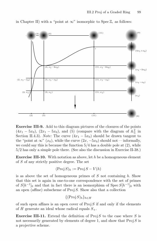
III.2 Proj of a Graded Ring 99
in Chapter II) with a “point at ∞” isomorphic to Spec Z, as follows:
(0)
(2, x1)
(2, x1−x0)
(3, x1)
(3, x1−x0)
(3, x1−2x0)
(11, x1)
(11, x1−x0)
(11, x1−2x0)
(x1)
(x1−x0)
(x1−2x0)
?(4x1+x0)
(2) (3) (11)
(2) (3) (11) (0)
Exercise III-9. Add to this diagram pictures of the closures of the points(4x1 − 5x0), (2x1 − 5x0), and (5) (compare with the diagram of A2
Z inSection II.4.3). Note: The curve (4x1 − 5x0) should be drawn tangent tothe “point at ∞” (x0), while the curve (2x, −5x0) should not— informally,we could say this is because the function 5/4 has a double pole at (2), while5/2 has only a simple pole there. (See also the discussion in Exercise II-38.)
Exercise III-10. With notation as above, let h be a homogeneous elementof S of any strictly positive degree. The set
(ProjS)h := ProjS − V (h)
is as above the set of homogeneous primes of S not containing h. Showthat this set is again in one-to-one correspondence with the set of primesof S[h−1]0 and that in fact there is an isomorphism of SpecS[h−1]0 withan open (affine) subscheme of ProjS. Show also that a collection
(ProjS)hh∈H
of such open affines is an open cover of ProjS if and only if the elementsof H generate an ideal whose radical equals S+.
Exercise III-11. Extend the definition of ProjS to the case where S isnot necessarily generated by elements of degree 1, and show that ProjS isa projective scheme.

100 III. Projective Schemes
Exercise III-12. Let S be a graded ring, not necessarily generated indegree 1. For any positive integer d, define the d-th Veronese subring of Sto be the graded ring
S(d) =∞⊕
ν=0
Sdν
Show that ProjS is isomorphic to ProjS(d). However, show that if S =A[x, y], then S(d) is not isomorphic to S as a graded algebra (or even as aring). Thus, as in the case of varieties, the correspondence between gradedalgebras and projective schemes is not one-to-one.
III.2.2 Closed Subschemes of Proj R
A homogeneous ideal I ⊂ A[x0, . . . , xr] determines a coherent sheaf of idealsI ⊂ OPr
A, and hence a closed subscheme of Pr
A. The following problemsdevelop these facts.
Exercise III-13. For each open set
Ui = (PrA)xi = Spec A[x0, . . . , xr, x
−1i ]0 ∼= Ar
A,
let I(Ui) be the ideal I ·A[x0, . . . , xr, x−1i ]∩A[x0, . . . , xr, x
−1i ]0. Show that
this definition may be extended in a unique way to other open sets U insuch a way that I becomes a coherent sheaf of ideals. We may thus speakof the closed subscheme V (I) of Pr
A associated to a homogeneous ideal I.
Exercise III-14. Conversely, given a closed subscheme X in PrA, we may
define a homogeneous ideal I(X) ⊂ A[x0, . . . , xr ] to be the ideal generatedby all homogeneous polynomials p(x0, . . . , xr) such that for every i settingthe i-th variable equal to 1 gives rise to an element
p(x0, . . . , 1, . . . , xr) ∈ JX(Ui) ⊂ A[x0, . . . , xr, x−1i ]0
Show that if I = I(X), then I = JX .
Note that with Exercise III-7 this shows that every closed subscheme of aprojective scheme is projective: if I ⊂ S = A[x0, . . . , xr] is a homogeneousideal, then V (I) ⊂ Pr
A is isomorphic to the scheme ProjS/I.
Exercise III-15. The correspondence between subschemes and ideals isnot, as it was in the case of affine schemes, one to one. For example, showthat in P1
K with K a field, the ideals I = (x0) and I ′ = (x20, x0x1) both
define the same reduced, one-point subscheme. More generally, show thatif I ⊂ S = K[x1, . . . , xr] is any homogeneous ideal, and for any integer n0
we define an ideal I ′ ⊂ I by
I ′ =⊕
n≥n0
In
then I and I ′ define the same subscheme of PrK .

III.2 Proj of a Graded Ring 101
Exercise III-16. To deal with this, define the saturation of a homoge-neous ideal J ⊂ S := A[x0, . . . , xr] to be the ideal
I = F ∈ S : F · Sn ⊂ J for some nand say that a homogeneous ideal is saturated if it equals its saturation.Show that there is a bijective correspondence between subschemes of Pr
A
and saturated ideals.
Exercise III-17. Show that the isomorphism of Exercise III-12 definesan isomorphism between projective space Pr
A and a closed subscheme ofPN−1
A , where N = dimA(A[x0, . . . , xr]d). (This is just the scheme-theoreticversion of the Veronese map.)
Exercise III-18. Show that if R is a graded ring finitely generated overa ring A = R0 (not necessarily generated by its graded part of degree 1),ProjR is isomorphic to a closed subscheme of some projective space Pr
A.
We conclude with a definition and a basic theorem.
Definition III-19. A morphism ϕ : X → Y of schemes is said to beprojective if it is the composition of a closed embedding X → Pn
Y with thestructure morphism Pn
Y → Y.
Note that if Y = Spec A is affine, this amounts to saying that X is of theform ProjS for some finitely generated A-algebra S. The basic fact aboutprojective morphisms is the one stated above:
Theorem III-20. Projective morphisms are proper.
For a proof see Hartshorne [1977, Theorem II.4.9].
Exercise III-21. Show that a finite morphism ϕ : X → Y is proper, andlocally projective in the sense that Y can be covered by open sets U ⊂ Ysuch that the restriction ϕ : V = ϕ−1U → U is projective. (We haveadopted the definition of projective morphism given in Hartshorne [1977,Section II.4]; what is here called locally projective is called projective byGrothendieck [1961, EGA II, 5.5].)
III.2.3 Global Proj
Proj of a Sheaf of Graded OX-Algebras. The construction of Proj ofa graded ring S gives rise to a scheme X = ProjS together with a structuremorphism X → B = Spec(S0). Because the association of ProjS to S isfunctorial, there is a more general construction that gives rise to schemes Xwith structure morphisms X → B to arbitrary schemes B, and that special-izes to the construction Proj when B is affine: all we have to do for generalB is replace the graded S0-algebra S with a sheaf of algebras over OB .
To carry this out, let B be any scheme. By a quasicoherent sheaf of gradedOB-algebras we will mean a quasicoherent sheaf F of algebras on B, and
102 III. Projective Schemes
a grading
F =∞⊕
ν=0
Fν
such that FνFµ ⊂ Fν+µ, and F0 = OB. Thus, for every affine open subsetU ⊂ B with coordinate ring A = OB(U), the ring F (U) will be a gradedA-algebra with 0-th graded piece F (U)0 = A.
Given such a sheaf F, for each affine open subset U ⊂ B we will letXU → U be the scheme XU = ProjF (U) with the structure morphismProjF (U) → Spec(A) = U. For every inclusion U ⊂ V of open subsetsof B, the restriction map F (V ) → F (U) is a homomorphism of gradedrings whose 0-th graded piece is the restriction map OB(V ) → OB(U), andso induces a map XU → XV commuting with the structure morphismsXU → U and XV → V and the inclusion U → V. We may thus gluetogether the schemes XU to arrive at a scheme X with structure morphismX → B; X is denoted ProjF ; and the construction of X is called globalProj.
As in the case of ordinary Proj, in most situations it will be the case thatthe sheaf of algebras F is generated by its first graded piece F1, and thatF1 is coherent (or, somewhat more generally, for some d > 0 the Veronesesubsheaf
F (d) =∞⊕
ν=0
Fdν
is generated by Fd, and Fd is coherent). Under these hypotheses it follows,again as in the case of ordinary Proj, that the morphism ProjF → B isproper.
The simplest example of global Proj gives us yet another construction ofprojective space over an arbitrary scheme S. Recall that projective spacePn
S over an arbitrary scheme S was defined initially in Chapter I via thegluing construction: if S is covered by affine schemes Uα = Spec Rα, wedefine projective space Pn
S to be the union of the projective spaces PnUα
,with the gluing maps induced by the identity maps on Uα ∩ Uβ. We canalso define it as a product:
PnS = Pn
Z ×SpecZ S.
Finally, we can realize it as the global Proj of the symmetric algebra of thefree sheaf of rank n + 1 on S:
Exercise III-22. Let S be any scheme. Show that projective space PnS
over S may be constructed as a global Proj:
PnS = Proj
(Sym(O⊕n+1
S )).
In particular, we can realize products of projective spaces over a givenscheme S either as fibered products, or via global Proj: if we denote by

III.2 Proj of a Graded Ring 103
OPnS[X0, . . . , Xm] the sheaf of graded OPn
S-algebras Sym(O⊕m+1
PnS
), then
PnS ×S Pm
S = ProjOPnS[X0, . . . , Xm].
A third way is via the Segre embedding:
Exercise III-23. Let S be any scheme. Show that
PnS ×S Pm
S∼= V
(Xi,jXk,l − Xi,lXk,j) ⊂ ProjOS [Xi,j0≤i≤n;0≤j≤m]
= P(n+1)(m+1)−1S .
This in turn gives us a way of describing subschemes of such a product,at least locally over the base:
Exercise III-24. Let S = Spec R be any affine scheme. Show that anyclosed subscheme
X ⊂ ProjR[x0, . . . , xn] ×S ProjR[y0, . . . , ym] = PnS ×S Pm
S
may be given as the zero locus of a collection Fα(x0, . . . , xn; y0, . . . , ym)of bihomogeneous polynomials Fα in the two sets of variables (x0, . . . , xn)and (y0, . . . , ym). In particular, show that the ideal of 2 × 2 minors of thematrix
(x0y0
x1y1
······
xn
yn
)defines the diagonal subset in Pn
S ×S PnS . Deduce that
any projective morphism is separated.
A more serious application of the global Proj construction is the defini-tion of the blow-up of a scheme X along a closed subscheme Y ⊂ X ; wewill discuss this in full in Chapter V. Another common use of global Proj isthe construction of the projectivization of a vector bundle, which we nowdescribe.
The Projectivization P(E ) of a Coherent Sheaf E . We saw in Exer-cise III-22 that projective space Pn
S over a scheme S is Proj(Sym(O⊕n+1S )).
We make a similar construction for any coherent sheaf E, and define theprojectivization P(E ) of E to be the B-scheme
P(E ) = Proj(Sym E ) −→ B.
To review the simplest case, let V be an n-dimensional vector space overa field K, regarded as a vector bundle over the one-point scheme Spec K.The projectivization of V is a projective space of dimension n over K. Theprojectivization of V ∗ is called the the dual projective space to PV. TheK-valued points of P(V ) correspond to one-dimensional quotients of V orequivalently to hyperplanes in V. The K-valued points of P(V ∗) correspondto one-dimensional subspaces of V ; this is what was classically called Pn.
More generally, if E is a locally free sheaf of rank n + 1, then P(E ) isa projective bundle over B, in the sense that for sufficiently small affineopen subsets U ⊂ B the inverse image of U in P(E ) is isomorphic to pro-jective space Pn
U as U -scheme. (When E is not locally free, it is less clearwhat the resulting scheme P(E ) will look like.) When B is a variety over
104 III. Projective Schemes
an algebraically closed field K and E the sheaf of sections of a vector bun-dle E on B, the K-valued points of P(E ∗) correspond to one-dimensionalsubspaces of fibers of E, while the K-valued points of P(E ) correspond toone-dimensional quotients of fibers of E, or equivalently to hyperplanes inthese fibers.
Note that any closed subscheme X ⊂ PnB may be realized as Proj(F ) for
some quasicoherent sheaf F of graded OB-algebras. More generally, if Eis any coherent sheaf, any closed subscheme X ⊂ P(E ) of its projectiviza-tion may be so realized. Conversely, if F is any quasicoherent sheaf ofgraded OB-algebras generated by F1, the surjection Sym(F1) → F givesan embedding X = ProjF → P(F1).
Exercise III-25. Let K be a field, P2K = ProjK[X, Y, Z] the projective
plane over K and (P2K)∗ = ProjK[A,B, C] the dual projective plane. Let
Σ be the universal line over (P2K)∗, that is,
Σ = V (AX + BY + CZ) ⊂ P2K ×K (P2
K)∗
viewed as a family over (P2K)∗. Show that Σ → (P2
K)∗ is the projectivizationof a locally free sheaf E of rank 2 on (P2
K)∗, and describe the sheaf E.
Exercise III-26. Let B be any scheme, E a locally free sheaf on B andE = Spec(SymE ∗) → B the total space of the vector bundle associatedto E. Show that we can complete E → B to a bundle of projective spacesover B: specifically, show that we have an inclusion on E in the bundleP(E ∗ ⊕OB) as an open subscheme, with complement a hyperplane bundleP(E ∗) ⊂ P(E ∗ ⊕ OB).
III.2.4 Tangent Spaces and Tangent Cones
Affine and Projective Tangent Spaces. The Zariski tangent spaces toa scheme are abstract vector spaces. When a scheme X over a field K isembedded in an ambient space like affine space or projective space overK, however, we can also associate to a point p of X with residue field K acorresponding linear subvariety of that affine or projective space, called theaffine tangent space or projective tangent space to X at p. In the case ofan affine scheme X = V (f1, . . . , fk) ⊂ An
K and point p = (a1, . . . , an) ∈ X,this is the subvariety given as
V
(∑i
∂fα
∂xi(a1, . . . , an) · (xi − ai)
α=1,...,k
).
To understand the relationship between this scheme and the Zariski tangentspace, note that a vector space over a field K is not the same thing as affinespace An
K . But it is true that, given a vector space V of dimension n overK, we may associate to V a scheme V, isomorphic to affine space An
K , sothat the points of V with residue field K correspond naturally to vectors

III.2 Proj of a Graded Ring 105
in V : this is just the spectrum of the symmetric algebra of the dual vectorspace
V = Spec (Sym(V ∗)) .
We will call V the scheme associated to the vector space V.This said, the scheme Tp(An
K) associated to the Zariski tangent space toaffine space An
K over a field K at any K-rational point p ∈ AnK (that is, a
closed point with residue field κ(p) = K) may be naturally identified withthe affine space itself, via an identification carrying the origin in Tp(An
K)to p. Now, suppose X ⊂ An
K is any subscheme, and p ∈ X any K-rationalpoint. The differential dιp of the inclusion ι : X → An
K at p represents theZariski tangent space Tp(X) as a vector subspace
dιp : Tp(X) → Tp(AnK).
We take the induced inclusion of schemes
dιp : Tp(X) → Tp(AnK) = An
K
and compose it with the translation morphism tp : AnK → An
K sending theorigin to p to obtain an inclusion
tp · dιp : Tp(X) → AnK −→ An
K .
The image of this inclusion is an affine subspace of AnK , which we will call
the affine tangent space to X at p. Again, note that it is a scheme, not avector space.
A similar construction will associate to a point p with residue field Kon a projective scheme X ⊂ Pn
K a linear space Tp(X) ⊂ PnK . One way to
do this is to choose an open subset U ∼= AnK ⊂ Pn
K containing p, and takethe closure in Pn
K of the affine tangent space to X ∩U at p. But there is amore intrinsic way. First, we write our ambient projective space Pn
K as theprojective space PV associated to a vector space V, that is, as
PnK = ProjS
whereS = SymV ∗
is the symmetric algebra of the dual of a vector space V. Thus, (k + 1)-dimensional linear subspaces of S1 = V correspond to k-planes in Pn
K . Welet
I = I(X) ⊂ S
be the homogeneous ideal of X ⊂ PnK , and let m = mp ⊂ S be the ideal of
forms vanishing at the point p ∈ X. Let J be the saturation of the idealI + m2 ⊂ S. We define the projective tangent space Tp(X) ⊂ Pn
K to X atp to be the subspace
Tp(X) = V (J ∩ S1) ⊂ PnK

106 III. Projective Schemes
of PnK . By way of explanation, note that J is the ideal of the first-order
neighborhood of p in X — that is, the intersection of X with the “fat point”P ⊂ Pn
K defined by the square of the ideal m of p. The projective tangentspace Tp(X) = V (J ∩ S1) is thus the span of this first-order neighborhoodV (J), that is, the smallest linear subspace of Pn
K containing V (J).
Exercise III-27. Show that this definition coincides with the naive defi-nition proposed initially.
Since the projective tangent space Tp(X) to a projective scheme X ata K-rational point p ∈ X is a linear subspace of the ambient projectivespace PV, it is of the form Tp(X) = PW for some quotient vector spaceV → W → 0. We may ask then what the relationship is between the vectorspace W and the Zariski tangent space Tp(X). The answer, which we willsee in Section VI.2.1 is that we have an exact sequence
0 −→ K −→ W ∗ −→ Tp(X) −→ 0.
More precisely, if V → U → 0 is the one-dimensional quotient of V cor-responding to the point p ∈ X ⊂ PV, then the surjection V → U factorsthrough a surjection ϕ : W → U, and we have a natural identification
Tp(X) = Hom(Kerϕ,U).
In any event, note that we do have a natural identification of the set oflines through p in Tp(X) with the set of lines through the origin in Tp(X).
Exercise III-28. Let X = V (F ) ⊂ PnK be the hypersurface in Pn
K givenby the homogeneous polynomial F (Z0, . . . , Zn), and let p = [a0, . . . , an] ∈X be any point with residue field K. Show that the projective tangentspace Tp(X) is the zero locus V (L) ⊂ Pn
K of the linear form
L(Z0, . . . , Zn) =n∑
k=0
∂F
∂Zi(a0, . . . , an) · Zk.
Tangent Cones. A more accurate reflection of the tangential behavior ofa scheme X at a point p ∈ X is its tangent cone. To define this, let X nowbe an arbitrary scheme, p ∈ X and point, OX,p the local ring of X at pand m = mX,p ⊂ OX,p the maximal ideal in OX,p. We define the tangentcone TCp(X) to X at p to be the scheme
TCp(X) = Spec( ∞⊕
α=0
mα/mα+1
).
A few observations about this construction are in order. First, we note thatthe graded ring B =
⊕(mα/mα+1) is generated by its first graded piece
B1 = m/m2 = (TpX)∗
so that B is a quotient of the ring
A = Sym((TpX)∗).

III.2 Proj of a Graded Ring 107
We thus have an inclusion
TCp(X) = Spec B → Spec A = TpX,
or in other words, the tangent cone to X at p is naturally a subscheme ofthe scheme associated to the Zariski tangent space TpX to X at p.
To give a more concrete realization of the tangent cone, suppose that Xis a subscheme of affine space over a field K, that is,
X ⊂ Spec K[x1, . . . , xn]
and let I = I(X) ⊂ K[x1, . . . , xn] be the ideal of X ; suppose moreoverthat the point p ∈ X is the origin (x1, . . . , xn) ∈ An
K . For any polynomialf ∈ K[x1, . . . , xn], write
f(x1, . . . , xn) = fm(x1, . . . , xn) + fm+1(x1, . . . , xn) + · · ·with fl(x1, . . . , xn) homogeneous of degree l and fm = 0; the first nonzeroterm fm(x1, . . . , xn) is called the leading term of f . Then we have thefollowing interpretation:
Exercise III-29. Show that the tangent cone
TCp(X) ⊂ TpX ⊂ Tp(AnK) = An
K
is the subscheme defined as the zero locus of the leading terms of all ele-ments f ∈ I.
Returning to the general case, note that since the ring B =⊕
(mα/mα+1)is graded, we can also associate a geometric object to the pair (X, p) bytaking ProjB. This is a subscheme of the projective space P(TpX) ∼= Pn
κ(p)
associated to the Zariski tangent space to X at p, called the projectivizedtangent cone to X at p and denoted PTCp(X). In many ways it is moreconvenient to deal with, being a projective scheme and of one lower dimen-sion than the tangent cone; it contains in general slightly less information(as exercise III-30 below will show, the tangent cone TCp(X) may have anembedded point at the origin, which the projectivized tangent cone willmiss).
Even though the degree of a general subscheme of projective space willnot be defined until Section III.3.1, we should mention here an importantinvariant of a scheme that can be defined in terms of the projectivizedtangent cone to X at p: we define the multiplicity of X at p to be thedegree of the projectivized tangent cone PTCp(X) ⊂ P(TpX) ∼= Pn
κ(p).This definition represents one more example of how schemes arise naturallyand are useful in the context of varieties: in the category of varieties wecan still define the tangent cone (as the reduced scheme associated to ourtangent cone) and projectivized tangent cone, but they do not behave wellin families.

108 III. Projective Schemes
There are many naturally occurring examples of nonreduced tangentcones. For example, consider the family of plane cubic curves with equationCt = Spec K[x, y]/(y2 − tx2 − x3) (that is, we let B = A1
K = Spec K[t],and take our family to be C = V (y2 − tx2 − x3) ⊂ A2
B → B). For each t,the curve Ct may be given parametrically as the image of the map
A1K = Spec K[λ] −→ A2
K = Spec K[x, y]
given by t → (λ2 − t, λ3 − tλ). For t = 0, this curve has a node at theorigin— the two points λ = ±√
t each map to the origin — and this isreflected in the tangent cone T(0,0)Ct = V (y2 − tx2), which is the union ofthe two lines y = ±√
t x. When t = 0, we see that the node of the curvehas degenerated to a cusp, and the tangent cone is now the double lineT(0,0)C0 = V (y2).
For more subtle examples, consider the curves C1 and C2 ⊂ A3K given
as the images of the maps νi : A1K → A3
K given by
ν1 : t −→ (t3, t4, t5)
andν2 : t −→ (t3, t5, t7).
In each case, let p be the singular point of Ci.
Exercise III-30. (a) Show that the projectivized tangent cones
PTCp(Ci) ⊂ P2K
to both curves Ci are curvilinear schemes of degree 3, that is, isomor-phic to Spec K[s]/(s3), and that they are not contained in any line inP2
K .
(b) Find an example of a curve C ⊂ A3K where the projectivized tangent
cone to C at the origin is isomorphic to Spec K[s]/(s3) and containedin a line.
(c) Find an example of a curve C ⊂ A3K where the projectivized tangent
cone to C at the origin is isomorphic to Spec K[s, t]/(s2, st, t2).
(d) Find an example of a curve C ⊂ A3K where the projectivized tangent
cone to C at the origin is contained in a line, but the Zariski tangentspace T0(C) is three-dimensional.
There is another geometric characterization of the tangent cone to ascheme X at a point p ∈ X : simply put, the tangent cone is the locus oflimiting positions of lines pq joining p to points q = p ∈ X as q approachesp. To state this precisely, suppose first that a neighborhood of p in Xis embedded in affine space An
K over a field K. Let T = TpAnK be the
affine space associated to the Zariski tangent space TpAnK to An
K at p, andconsider the incidence correspondence
Σ =(v, q) : v ∈ T p(pq) ⊂ T × (An
K \ p).

III.2 Proj of a Graded Ring 109
Equivalently, in terms of the identification of T with AnK itself, Σ is the
subscheme of AnK × (An
K \ p) given by the equations
yi
(xj − xj(p)
)− yj
(xi − xi(p)
)= 0.
Let Γ = π−12 (X \ p) ⊂ T × (X \ p) be the inverse image of X \ p in
Σ, and Γ the closure of Γ in T × X. We have then:
Proposition III-31. The tangent cone TCpX is the fiber of Γ over thepoint p ∈ X.
This statement (modulo possible embedded components at the origin inTCpX) will be proved in Chapter IV. It amounts to the statement thatthe projectivization of TCpX is the exceptional divisor of the blow-up ofX at p.
Proposition III-31 is very useful, for example in doing Exercises III-32-III-34 below.
Exercise III-32. Let V be the vector space of polynomials of degree n onP1
K = ProjK[X, Y ], that is, homogeneous polynomials of degree n in twovariables X, Y, and let PV ∗ ∼= Pn
K be the projective space parametrizingone-dimensional subspaces of V. Let ∆ ⊂ Pn
K be the discriminant hyper-surface, that is, the locus of polynomials with a repeated factor with thereduced scheme structure (we will see in Chapter V how to give equationsfor, and hence a natural scheme structure on, ∆). If
F (X, Y ) =∏
(aiX + biY )mi
is any polynomial of degree n (with the factors aiX +biY pairwise indepen-dent), what is the support of the tangent cone to ∆ at the point p = [F ]?(Hint: consider lines in Pn
K through the point [F ]. How many other pointsof intersection with ∆ will a general such line have, and which lines willhave fewer?)
Exercise III-33. More generally, suppose ∆m ⊂ PnK is the locus of poly-
nomials with an m-fold root. Again, what is the support of the tangentcone to ∆m at a point [F ], where F is as above?
Exercise III-34. This is an exercise from classical geometry. Suppose C ⊂Pn
K is a nonsingular curve. The union of the projective tangent lines to Cis the support of a surface S ⊂ Pn
K , called the tangent developable to C;this surface will be singular along C (see Harris [1995] for example). Whatis the support of its tangent cone at a general point p ∈ C? (Note that ifwe take C to be the rational normal curve in Pn
K , that is, the image of then-th Veronese map P1
K → PnK , then this is a special case of exercise III-33
above.)
Exercise III-35. In each of the following, a finite group G acts on theaffine plane A2
K = Spec K[x, y]. The quotient A2K/G (that is, Spec K[x, y]G)

110 III. Projective Schemes
will have a singularity at the image of the origin (x, y) ∈ A2K . Describe the
tangent cone in each case.
(a) G = Z/(3), acting by (x, y) → (ζx, ζy), where ζ is a cube root of unity.
(b) G = Z/(3), acting by (x, y) → (ζx, ζ2y), where ζ is a cube root ofunity.
(c) G = Z/(5), acting by (x, y) → (ζx, ζy), where ζ is a fifth root of unity.
We will encounter tangent cones again in our discussion of blowing up:as we indicated, the projectivized tangent cone PTCp(X) to a scheme Xat a point p ∈ X is the exceptional divisor in the blow-up Blp(X) of X atp. In particular, tangent cones to arithmetic schemes will come up again inthis way in Section IV.2.4.
III.2.5 Morphisms to Projective Space
Just as there is a simple characterization of morphisms to an affine scheme(Theorem I-40), there is a simple way of viewing morphisms to projectivespace in terms of line bundles, or, equivalently, invertible sheaves, a conceptwe will introduce in this section. Invertible sheaves have another geometricrealization in the notion of Cartier divisors, and we will describe this con-nection as well. See Hartshorne [1977, Chapter II] for further information.
If we understand morphisms to the scheme PnA, we will understand mor-
phisms to an arbitrary projective scheme Y ⊂ PnA, since a morphism to Y
is just a morphism to PnA that factors through Y (a sharp version of this is
given in Exercise III-45); thus we will study morphisms to projective space.To understand the situation, we first consider morphisms ϕ : X → Pn
A =ProjA[x0, . . . , xn] in the category of A-schemes, where X = Spec K is thespectrum of a field. Since X has only one point, the image p of such amorphism must be contained in one of the open sets
Ui = (PnA)xi = Spec A
[x0
xi, . . . ,
xn
xi
] ∼= AnA.
Thus the map corresponds to an n-tuple of scalars (a0, . . . , ai, . . . , an) ∈Kn. Of course, p may also be contained in another open set Uj ; in this caseaj = 0 and the coordinates in Uj are
(b0, . . . , bj , . . . , bn) =(a0
aj, . . . ,
1aj
. . . ,an
aj
).
To show the coordinates without prejudice toward one or another of theUi, we may say that a map Spec K → Pn
A corresponds to an (n+1)-tupleof elements of K, not all zero, with two such (n+1)-tuples correspondingto the same map if and only if they differ by a scalar; the map abovecorresponds to the (n+1)-tuple [α0 =a0, . . . , αi =1, . . . , αn =an], or, equiv-alently, [β0 =b0, . . . , βj =1, . . . , βn =bn].

III.2 Proj of a Graded Ring 111
Having said this, we may extend exactly the same consideration to thecase of a morphism X → Pn
A, where X is the spectrum of a local A-algebra:
Proposition III-36. If T is a local A-algebra, the morphisms Spec T →Pn
A (in the category of A-schemes) are in one-to-one correspondence withthe set of (n+1)-tuples [α0, . . . , αn] ∈ T n+1 such that at least one of the αi
is a unit, modulo the equivalence relation [α0, . . . , αn] ∼ [αα0, . . . , ααn] forany unit α ∈ T .
Proof. Write PnA = ProjA[x0, . . . , xn]. Given an (n+1)-tuple [α0, . . . , αn]
with αi a unit, we map Spec T to Ui = (PnA)xi ⊂ Pn
A via the map corre-sponding to the A-algebra homomorphism[x0
xi, . . . ,
xn
xi
]−→ T,
xj
xi −→ αj
αi.
Conversely, given a morphism ϕ : Spec T → PnA of A-schemes, let p ∈
Spec T be the unique closed point, and suppose that ϕ(p) ∈ Ui. The preim-age ϕ−1(Ui) is an open subset of Spec T containing p, and hence in all ofSpec T ; in other words, ϕ(X) ⊂ Ui. The map ϕ is thus given by a map ofA-algebras [x0
xi, . . . ,
xn
xi
]→ T
and we may associate to ϕ the (n+1)-tuple[α0 =
x0
xi, . . . , αi =1, . . . , αn =
xn
xi
].
(If the image ϕ(x) is also contained in Uj, we arrive at the (n+1)-tuple[β0 =
x0
xj, . . . , βj =1, . . . , αn =
xn
xj
],
which equals [αα0, . . . , ααn] for α = xi/xj .)
To generalize this further, to affine rings or schemes, we seek a construc-tion that, locally, reduces to the one above. To this end, we may regard the(n+1)-tuple (α0, . . . , αn) of the proposition as giving a module homomor-phism
α : T n+1 → T.
To say that α is surjective is equivalent to saying that any of the αi is aunit in T . And two such maps are equivalent if they differ by compositionwith an automorphism of the module T (that is, multiplication by a unit).Equivalently, the kernel is a rank-n summand of T n+1.
It turns out that this last sentence generalizes to describe A-morphismsfrom an A-scheme X to Pn: they correspond to subsheaves E ⊂ On+1
X ofrank n that are locally direct summands of On+1
X ; or, equivalently, to maps
On+1X → P → 0,

112 III. Projective Schemes
where P is a sheaf locally isomorphic to OX (such a sheaf is called invertible,a term that will be explained in the following discussion), modulo units ofOX acting as automorphisms of P .
Theorem III-37. For any scheme X, we have natural bijections
Mor(X, PnZ)
= subsheaves K ⊂ On+1X that locally are summands of rank n
=invertible sheaves P on X, together with an epimorphism On+1
X →Punits of OX(X) acting as automorphisms of P .
Here “natural” means that for any morphism ϕ : X → Y of schemes, themap Mor(Y, Pn
Z) → Mor(X, PnZ) given by composition with ϕ commutes
with pullback of invertible sheaves and epimorphisms; in other words, wehave an isomorphism of functors from the category of schemes to the cat-egory of sets.
Of course, if X → B is a B-scheme, we will be interested in describingthe morphisms of X to Pn
B over B. This turns out to involve no new ideas:somewhat surprisingly, for any B-scheme X → B, a B-morphism X → Pn
B
is exactly the same thing as a morphism X → PnZ ! The point is, since Pn
B isthe product of Pn
Z with B, a morphism of any scheme X to PnB is uniquely
determined by the data of a morphism X → B and a morphism X → PnZ.
X ............................ PnB
B Pn
Z
Spec Z
Thus, after specifying a structure morphism ϕ : X → B we get a bijection
Mor(X, PnZ) ↔ MorB(X, Pn
B).
We now proceed with the proof of Theorem III-37. Because all the termsin these equalities are defined locally on X, the theorem reduces easily tothe case where X is affine, and this is the case we will actually prove below.First, we review the corresponding notions about modules. A good basicreference is Bourbaki [1972, Chap. II-5].
Recall that a module K over a ring T is locally free of rank m if for everymaximal ideal (or, equivalently, every prime ideal) p the Tp-module Kp isfree of rank m. This is the same as the sheaf-theoretic notion.
Exercise III-38. Let K be a finitely generated module over a Noetherianring T, and let K be the corresponding coherent sheaf over Spec T. Showthat K is a locally free module in the sense above if and only if K is a locally

III.2 Proj of a Graded Ring 113
free coherent sheaf in the sense that there is an affine cover of Spec T bybasic open sets Spec Tfi such that the restriction of K to each of these setsis free (equivalently, each K[f−1
i ] is free over Tfi = T [f−1i ]).
An invertible T -module is a finitely generated, locally free T -module ofrank 1.
In commutative algebra, locally free modules are usually called projectivemodules; their characteristic property is that if P is a locally free T -module,then any epimorphism of T -modules M →→ P splits. It follows that ifK ⊂ T n+1 is a submodule, then K is a summand of T n+1 if and only ifT n+1/K is a locally free module; in particular, K is a rank n summand ofT n+1 if and only if T n+1/K is an invertible module.
Before giving the proof of Theorem III-37, we record a result that comesfrom an immediate application of the definitions.
Proposition III-39. A morphism of an arbitrary scheme X to projectivespace Pr
Z = ProjZ[x0, . . . , xr] may be given by a collection of maps ϕi :Ui → (Pr
Z)xi , where Ui is an open cover of X, the (PrZ)xi ⊂ Pr
Z are theopen subsets of Exercise III-6, and the maps ϕi and ϕj induce the samemap Ui ∩ Uj → (Pr
Z)xi ∩ (PrZ)xj = Spec(Z[x0, . . . , xr][x−1
i , x−1j ])0.
The heart of Theorem III-37 is the following result, which is the affineversion of the first equality.
Proposition III-40. If T is any ring, then
Mor(Spec T, PnZ)
= K ⊂ T n+1 | K is locally a rank n direct summand of T n+1.
Proof. Suppose, first, that K is a rank n free summand of T n+1, and writeP for the module T n+1/K. This module is locally free of rank 1 and isgenerated by the n + 1 images ei of the n + 1 generators of T n+1. Let Ij
be the annihilator of (P/Tej), and let Uj be the complement of V (Ij) inSpec T, so that the Uj form an open cover of Spec T. Regard T -modulesas sheaves on Spec T. On Uj the map T → P defined by 1 → ej is anisomorphism, and identifying P |Uj with T |Uj via this map, the projec-tion T n+1|Uj → (T n+1/K)|Uj = P |Uj = T |Uj has a matrix of the form(tj0, . . . , tjj = 1, . . . , tjn), which defines an element of T n+1
Ujand thus a
morphism Spec T → AnZ . These morphisms agree on overlaps as in Propo-
sition III-39, so they define a morphism Spec T → PnZ .
Conversely, suppose that we are given a morphism ψ from Spec T toPn
Z . Since PnZ is covered by n + 1 affine n-spaces, ψ is by definition asso-
ciated to an open cover Spec T =⋃
i=0,...,n Ui and for each j an element(tj0, . . . , tjj = 1, . . . , tjn) of T n+1|Uj such that tij is a unit on Ui ∩ Uj andtil = tijtjl in T |Ui∩Uj for all i, j, l. Two such T -valued points are the sameif and only if the corresponding elements of T n+1|Uj are equal for each j.

114 III. Projective Schemes
Let Kj be the kernel of the map T n+1|Uj → T |Uj defined by the matrix(tj0, . . . , tjj = 1, . . . , tjn), and let
K = a ∈ T n+1 : a|Uj ∈ Kj for each j.To see that K is locally a rank n summand of T n+1, note that any
local ring of T is a local ring of one of the Uj so the result of localizingthe sequence 0 → K → T n+1 → T n+1/K → 0 at any prime ideal p is asequence of the form
0 → Kp → T n+1p → Tp → 0,
and such a sequence must split.
Exercise III-41. The word “locally” can be omitted in the statement ofthe proposition, because a submodule of a finitely generated free modulethat is locally a direct summand is in fact a direct summand. Prove this.
To derive a version of this with invertible modules, we use the fact thatK ⊂ T n+1 is a direct summand of rank n if and only if T n+1/K is aninvertible module, and identify the set on the right-hand side of the equalityin Proposition III-40 with the set of invertible quotient modules of T n+1.We may separate the isomorphism class of the quotient from the surjectionthat makes it a quotient and look at invertible T -modules P with surjectionsT n+1 → P. Two surjections α, β : T n+1 → P have the same kernel if andonly if there is an automorphism σ : P → P such that β = σα. But ifP is an invertible T -module, then HomT (P, P ) = T (reason: the naturalmap α : T → HomT (P, P ) taking 1 to the identity is locally the same asthe natural map T → HomT (T, T ), which is an isomorphism, so α is anisomorphism). Thus the automorphisms of P may be identified with unitsof T, and we get the following corollary:
Corollary III-42. If T is any ring, then
Mor(Spec T, PnZ)
=
invertible T -modules P with an epimorphism T n+1 → P
isomorphisms ,
where an isomorphism from ϕ : T n+1 → P to ϕ′ : T n+1 → P is anisomorphism α : P → P ′ such that αϕ = ϕ′. Note that the set of such iso-morphisms is either empty or in (non-natural) one-to-one correspondencewith the units of T .
In the classical case of the variety PnK over a field K, we can specify points
of PnK by giving (n+1)-tuples of elements of K, not all zero. (In the scheme
PnK , of course, there are other, nonclosed points as well.) Analogously, for
any ring A, an (n + 1)-tuple (a0, . . . , an) of elements ai ∈ A that generatethe unit ideal defines a surjection An+1 → A of A-modules and thus definesan A-valued point of Pn
A.

III.2 Proj of a Graded Ring 115
Exercise III-43. (a) Show that there are bijections between the sets(n + 1)-tuples of elements of A that generate the unit ideal
and
maps Spec A → PnA such that the composite Spec A → Pn
A → Spec Ais the identity (A-valued points of Pn
A in the category of A-schemes)
.
(b) Show that the image of the morphism SpecA → PnA associated to an
(n + 1)-tuple (a0, . . . , an) is the closed subscheme
V (aiXj − ajXi0≤i,j≤n).
If A is a domain, show that (aiXj − ajXi0≤i,j≤n) is a prime ideal.
If A is a domain, Exercise III-43 shows that the image is a reduced andirreducible closed subscheme of Pn
A, and in particular corresponds to a pointof |Pn
A|. The example of the point of P1Z corresponding to (2, 5) is treated
in Exercise III-9 above. Note that the Spec Z-valued point (2, 5) is not aSpec Z-valued point of either open set in the standard affine open coverP1
Z = A1Z ∪A1
Z of P1Z, even though the point (2x1−5x0) ∈ |P 1
Z | lies in both!Finally, if we are working in the category of B-schemes, we may ask for
a generalization of this result describing maps of a given B-scheme X to aprojective bundle. To state the result, let E be any coherent sheaf on B.We have then:
Theorem III-44. For any B-scheme ϕ : X → B and coherent sheaf E onB, there is a natural bijection
MorB(X, P(E ))
=invertible sheaves P on X, together with an epimorphism ϕ∗E → P
isomorphisms ,
where isomorphism is defined as in Corollary III-42.
We will not prove this here; the proof can be carried out by locallyexpressing the coherent sheaf E as a quotient of a free sheaf On+1
B , andcharacterizing the subset of morphisms from X to Pn
B that factor throughthe resulting inclusion P(E ) → Pn
B.
Exercise III-45. (a) Suppose that Y ⊂ PnA is the closed subscheme de-
fined by homogeneous equations Fi. If T is a local A-algebra then, aswe showed above, the morphisms from Spec T to Pn
A may be identifiedwith n + 1-tuples of elements of T generating the unit ideal, modulounits of T. Show that the condition that such an n+1-tuple correspondto a map to Y is simply that it be a zero of all the polynomials Fi.
(b) The general case of a map from an affine A-scheme to a projective A-scheme can be reduced to the local one using the following fact: if T isany A-algebra a morphism Spec T → Pn
A factors through X if and onlyif for all primes p of T the composite morphisms Spec Tp → Spec T →Pn
A; factor through X. Prove this.

116 III. Projective Schemes
Having characterized morphisms of schemes to projective spaces, it isinstructive to look back to other geometric theories for similar characteri-zations. Recall that in topology the space Pn
C of n-dimensional subspacesof a complex (n+1)-dimensional vector space Cn+1 is the classifying spacefor subbundles of rank n of a trivial bundle of rank n+1 (and similarly forPn
R). This means that for all spaces X, maps X → PnC correspond to the
rank n subbundles of the trivial bundle on X. The correspondence is easyto describe: a rank n subbundle J of the trivial bundle V = Cn+1 ×X onX corresponds to the map X → Pn
C that sends a point p ∈ X to the pointof Pn
C corresponding to the space
Jp ⊂ Vp = Cn × p = Cn.
There are other equivalent descriptions, which may be more familiar, interms of the rank 1 quotient bundle V /J or the subbundle (V /J )∗ ⊂ V ∗
of rank 1.Analogous results hold in the category of complex analytic spaces and
maps and in the category of algebraic varieties and regular maps (takingthe subbundles to be complex analytic, or algebraic, respectively). In thissection we give a corresponding result for schemes. The main difference isthat in algebraic geometry, it is traditional to replace vector bundles on Yby their sheaves of sections.
To see what these sheaves should look like, consider first that if E isa trivial vector bundle of rank 1 on a scheme X , then a section of E isthe same as a function on X , so the sheaf of sections of E should be OX .Taking direct sums, we see that the sheaf of sections of a trivial vectorbundle of rank m is the coherent sheaf that is the free OX -module Om
X . Ingeneral, since vector bundles are by definition locally trivial, their sheavesof sections are locally free sheaves of OX -modules of finite rank — locallyfree coherent sheaves. It is not hard to go in the other direction as well andto derive from a locally free coherent sheaf a vector bundle.
Given this equivalence between vector bundles and locally free coherentsheaves, why work with locally free sheaves? The reason is similar to thereason for working with schemes instead of varieties even if one is primarilyinterested in varieties: locally free coherent sheaves live naturally in thelarger category of coherent sheaves, and working in the larger categorygives us flexibility. Standard constructions in the smaller category (suchas taking the fibers of a morphism of schemes, or taking the cokernel ofa homomorphism of locally free sheaves) are most naturally interpreted inthe larger category.
Like the line bundles to which they correspond, locally free sheaves ofrank 1 play an especially important role and have a special name: they arecalled invertible sheaves. The terminology comes from number theory: aninvertible module over a domain T is a finitely generated submodule I ofthe quotient field such that, for some other finitely generated submoduleJ of the quotient field (called its inverse) we have IJ = T, the unit ideal.

III.2 Proj of a Graded Ring 117
Over the scheme Spec T, the corresponding sheaf is an invertible sheaf.More generally, given any invertible sheaf I over an arbitrary scheme X,the sheaf I ∗ = Hom(I , OX) is again invertible and the natural map I ⊗I ∗ → OX is an isomorphism (check locally). For this reason I ∗ is calledthe inverse of I .
Knowing that invertible sheaves correspond to line bundles does not atfirst seem to help connect them to geometry. Just as in classical algebraicgeometry, however, morphisms of a scheme X to projective space can in factbe characterized in geometric terms using the related notion of an effectiveCartier divisor. This is defined to be a subscheme D ⊂ X such that at everypoint x ∈ X the ideal of D in the local ring OX,x is principal and generatedby a nonzerodivisor. In other words, a subscheme D is an effective Cartierdivisor if and only if its ideal sheaf ID is invertible. Following tradition,we define the invertible sheaf OX(D) associated to D to be the inverse
OX(D) = I ∗D.
The invertible sheaves form a group PicX under the tensor product oper-ation, and under reasonable circumstances— for example, for subschemesof projective space over a field— every invertible sheaf can be written asOX(D)⊗IE = OX(D)⊗OX(E)∗ for some effective Cartier divisors D, E.
Note the unfortunate but essentially unambiguous notation: if U is anopen set of X then O(U) denotes the ring of sections of the sheaf OX definedover U , while if D is a Cartier divisor O(D) denotes the sheaf above. Ofcourse we could also manufacture such monstrosities as OX(D)(U). . . .
We may tighten the connection between invertible sheaves and effectiveCartier divisors as follows: If D is an effective Cartier divisor then theinclusion ID → OX is a global section of Hom(ID, OX) = OX(D). Thissection is regular in the sense that for every open set U ⊂ X no nonzeroelement of OX(U) annihilates the restriction of this section to U (Reason:the image of ID(U) in OX(U) contains a nonzerodivisor.) Thus an effectiveCartier divisor gives rise to an invertible sheaf with a global section.
Conversely, given an invertible sheaf L and a global section σ, we definethe zero locus of that section to be the support of the quotient L /OXσ.To understand what this means, choose a covering of X by open sets Usuch that L |U ∼= OU . The zero locus of σ in U is then the zero locus of thecorresponding element of OU . If the section is regular, it follows that thezero locus is an effective Cartier divisor. Note that another global sectiondiffering from σ by a unit in OX(X) would give the same Cartier divisor.We thus have a bijection
effective Cartier divisors
invertible sheaves with choice of global section modulo units .
The reader might wonder about the significance of “effective”. An ef-fective Cartier divisor D may be defined by giving a nonzerodivisor in

118 III. Projective Schemes
fU ∈ OX(U) for each set U of an open covering of X , and fU is defined upto a unit of OX(U). Thus D gives rise to a unique global section of the sheafof invertible rational functions modulo invertible regular functions—thatis, the sheaf M ∗
X/O∗X , where ∗ denotes the sheaf of multiplicative units,
and MX is the sheafification of the presheaf whose value on an open set Uis the localization OX(U)[S−1
U ] of the ring OX(U) at the multiplicativelyclosed set SU of elements that become nonzerodivisors in OX,x for everyx ∈ U . (All that one usually needs to know about this slightly baroque def-inition is that if U = Spec A for a Noetherian ring A, then MX(U) is theresult of inverting all nonzerodivisors in A. More general cases are subtle;see for example Kleiman [1979] for information.) We define a Cartier divi-sor in general to be an arbitrary section of the sheaf M ∗
X/O∗X . The Cartier
divisors on X form a group called Div X , and the association D → OX(D)defines a homomorphism Div X → PicX.
The effective Cartier divisors form a monoid in Div X ; again, in reason-able circumstances such as for subschemes of a projective space over a field,the monoid of effective Cartier divisors generates Div X , and in the freestpossible way: Div X may also be realized as the Grothendieck group of themonoid. The effective Cartier divisors are then just the Cartier divisorsthat “effectively” define subschemes.
III.2.6 Graded Modules and Sheaves
The attentive reader may have noticed that Theorem III-37 implies theexistence of a distinguished invertible sheaf on Pn
Z , namely, the one corre-sponding to the identity map. In this section we will give descriptions ofthis sheaf, which plays a fundamental role in projective geometry.
We begin with a general method for constructing sheaves on schemesof the form ProjA analogous to the construction of sheaves on SpecAfrom modules over A. Let B be a scheme, and let A = A0 ⊕ A1 ⊕ · · ·be a quasicoherent sheaf of graded OB-algebras. Let P = ProjA . Let Mbe a quasicoherent sheaf on B which has the additional structure of asheaf of graded A -modules; that is, we have a direct sum decompositionM = · · ·⊕Mi⊕Mi+1⊕· · · and there are maps Ai⊗Mj → Mi+j satisfyingthe usual axioms (associativity, identity, . . . ). We may associate to M aquasicoherent sheaf M on P as follows: Let U be an affine subset of B,and consider the graded ring A (U). For each homogeneous element f ofA (U) we have an affine open set PU,f := (ProjA (U))f = Spec(A (U)f )0of P; the schemes PU,f form an affine open cover of P. The sections M (U)over U form a graded module over the graded ring A (U). Let MU,f bethe (A (U)f )0-module MU,f = (M (U) ⊗A (U) A (U)[f−1])0, and let M U,f
the corresponding sheaf on the affine scheme PU,f . These patch togetherto define a quasicoherent sheaf on P that we denote by M .
In fact, every quasicoherent sheaf on ProjA corresponds to a sheaf ofgraded A modules in this way. However, unlike the correspondence between

III.2 Proj of a Graded Ring 119
modules over a ring and quasicoherent sheaves over Spec of that ring, thecorrespondence is not bijective. For example, as the reader can easily check,the sheaf associated to a module M is the same as the sheaf associated tothe truncated module M ′ = ⊕n≥n0Mn for any n0. But in good cases thisis the only kind of failure: for example, the association M → M gives abijection
sheaves of finitely generated graded A -modules up to truncation
quasicoherent sheaves on P .
To start with the simplest example, if we take M = A we get the struc-ture sheaf OP . Much more interesting is the deceptively simple modificationobtained by shifting the grading by 1. In general, if M =
⊕i Mi then we
define the n-th twist M (n) of M to be the same module but with degreesshifted by n, that is
M (n)i = Mn+i.
We define OP(n) to be the sheaf A (n) associated to the sheaf of gradedmodules A (n). The most important of these is OP(1), called the tautologicalsheaf on P.
Exercise III-46. Assume the algebra A is generated in degree 1. Showthat all the sheaves OP(n) are invertible. Show that OP(n) ⊗ OP(m) =OP(n + m), and in particular OP(n)−1 = OP(n)∗ = OP(−n).
Exercise III-47. Let π : ProjA → Spec A0 be the structure map. Showthat for any quasicoherent sheaf N on Spec A0 the pullback π∗(N ) is thesheaf assocated to A ⊗A0 N .
Exercise III-48. Let K be a field, and consider the projective space PnK =
ProjK[x0, . . . , xn]. Let H be a hyperplane. Show that H is a Cartier divisoron Pn
K and that the associated invertible sheaf is OPnK
(1).
III.2.7 Grassmannians
Grassmannians exist in the category of schemes, and behave very muchlike Grassmannians in classical algebraic geometry. More precisely, thereis, for any scheme S and positive integers n and k < n, a scheme GS(k, n)called the Grassmannian over S; the construction is functorial in S, in thesense that for any morphism T → S, the Grassmannian GT (k, n) is thefiber product GS(k, n) ×S T. (In particular, there is a scheme GZ(k, n)—the Grassmannian over Spec Z — such that any Grassmannian may be re-alized as GS(k, n) = GZ(k, n) × S.) Moreover, in case S = Spec K is thespectrum of an algebraically closed field the scheme GS(k, n) is the schemeassociated to the classical Grassmann variety G(k, n) over K. In fact, theconstructions, which we will describe briefly below, are themselves exactly

120 III. Projective Schemes
analogous to the standard constructions of the Grassmannian in the clas-sical context. Rather, as in the case of projective space, what is new anddifferent about the Grassmannian as a scheme are the subschemes of it; wewill illustrate this with our discussion of Fano schemes below.
We will begin with the constructions of the Grassmannian GS(k, n) forS = Spec A an affine scheme (this is also called the Grassmannian over Aand denoted GA(k, n)). At the end, we will observe that the constructionis natural, in the sense that for any morphism T → S of affine schemes wehave
GT (k, n) = GS(k, n) ×S T.
It will follow that we can construct Grassmannians over arbitrary schemesS by gluing together the Grassmannians GUα(k, n) over a collection of affineopen subsets Uα ⊂ S covering S. Alternatively, we can simply carry outthe construction of the Grassmannian GZ(k, n) over Spec Z, and then forany scheme S simply define GS(k, n) = S × GZ(k, n).
In the classical setting, there are two ways of constructing the Grass-mannian GK(k, n) as a variety over a field K. Abstractly, we may describeGK(k, n) as a union of open sets, each isomorphic to affine space Ak(n−k)
K .Alternatively, we may describe it at one stroke as the closed subvariety ofprojective space PN
K given by the Plucker equations. Each of these construc-tions has an immediate extension to the category of schemes, and they doyield the same object. Moreover, there is in the language of schemes a thirdway to characterize Grassmannians: as Hilbert schemes, or more preciselyas the schemes representing the functors of families of linear subspaces of afixed vector space. We will discuss this third construction in Section VI.2.1.This is in many ways the optimal characterization of the Grassmannian: itavoids the extraneous introduction of coordinates, gives us immediately adescription of morphisms of an arbitrary scheme Z to GK(k, n), and givesus a natural definition of equations for subschemes of the Grassmanniansuch as Fano schemes and more general Hilbert schemes.
We will start by reviewing the gluing construction of the Grassmannianas a variety over a field. We begin by realizing the set of k-dimensionallinear subspaces Λ of the n-dimensional vector space Kn over a field K asthe set of k×n matrices M of rank k, modulo multiplication on the left byinvertible k × k matrices. For each subset I ⊂ 1, 2, . . . , n of cardinality kwe can multiply any matrix M whose I-th minor is nonzero by the inverseof its I-th submatrix MI , to obtain a matrix M ′ with I-th submatrix equalto the identity. In this way, we may identify the subset UI ⊂ GK(k, n)of planes Λ complementary to the subspace of Kn spanned by the basisvectors eii/∈I with the affine space Ak(n−k)
K whose coordinates are theremaining entries of M ′. We thus have the following recipe for the varietyGK(k, n):
Let W ∼= AknK be the space of k × n matrices, and for each subset I ⊂
1, 2, . . . , n of cardinality k, let WI ⊂ W be the closed subset of matrices
III.2 Proj of a Graded Ring 121
with I-th submatrix equal to the identity. For each I and J = I, let WI,J ⊂WI be the open subset of matrices whose J th minor is nonzero; let ϕI,J :WI,J → WJ,I be the isomorphism given by multiplication on the left by MJ ·M−1
I . We then define the Grassmannian GK(k, n) as an abstract variety tobe the union of the affine spaces WI
∼= Ak(n−k)K modulo the identifications
of WI,J with WJ,I given by ϕI,J .This recipe applies perfectly well to define the Grassmannian GS(k, n)
over any affine scheme S = Spec A, using the gluing construction of Sec-tion I.2.4: let
W = Spec A[ . . . , xi,j , . . . ] ∼= AknS ,
and for each subset I = (i1, . . . , ik) ⊂ 1, 2, . . . , n let WI ⊂ W be theclosed subscheme corresponding to matrices whose I-th k× k submatrix isthe identity; that is, the zero locus of the ideal (. . . , xα,iβ
− δα,β , . . .). Foreach I and J = I, we define exactly as before open subschemes WI,J =(WI)det Mj ⊂ WI and isomorphisms ϕI,J : WI,J → WJ,I ; and we thendefine the Grassmannian GS(k, n) to be the S-scheme obtained by gluingthe affine spaces WI
∼= Ak(n−k)S along the ϕI,J .
An alternative construction of the Grassmannian GS(k, n) is as a sub-scheme of projective space PN
S , where N =(
nk
) − 1, given by the Pluckerequations. Again, if we are simply careful about transcribing the classicalconstruction, it works in this new setting as well.
To set it up, start with the polynomial ring A[ . . . , XI , . . . ] in(
nk
)vari-
ables over A, where the variables are labeled by subsets I = (i1 < · · ·< ik)⊂1, . . . , n. We may think of the variables XI as corresponding to the max-imal minors of a k × n matrix M. If we specify further that the first k × ksubmatrix of M is the identity — that is, M is of the form (Ik, B) whereB is a k× (n− k) matrix— then these are in turn up to sign the minors ofall sizes of the matrix B. For example, the (i, l)-th entry of B is the I-thminor of M, where I = (1, 2, . . . , ı, . . . , k, k + l); the ((i, j), (l, m))-th minorof B is the I-th minor of M, where I = (1, 2, . . . , ı, . . . , j, . . . , k, k+l, k+m);and so on.
In terms of this description of the coordinates XI as the minors of all sizesof a k × (n − k) matrix A, the Plucker relations are simply homogeneouspolynomials in the variables XI obtained by expanding the determinantsof these submatrices in terms of products of complementary minors of com-plementary submatrices. For example, Cramer’s rule translates into an ex-pression of the determinant of an l× l submatrix of A as a sum of productsof entries and determinants of (l − 1) × (l − 1) submatrices; in particular,on the basis of the identification made above we have the relation
−X(1,2,...,ı,...,j,...,k,k+l,k+m)X(1,2,...,k)
= X(1,2,...,ı,...,k,k+l)X(1,2,...,j,...,k,k+m) −X(1,2,...,ı,...,k,k+m)X(1,2,...,j,...,k,k+l).
We take the Plucker ideal J ⊂ A[ . . . , XI , . . . ] to be the ideal generated bythe Plucker relations.

122 III. Projective Schemes
Another, more intrinsic way to describe the ideal J is simply this: we letϕ be the map
A[ . . . , XI , . . . ] −→ A[x1,1, . . . , xk,n]
XI −→
∣∣∣∣∣∣∣x1,i1 . . . x1,ik
......
xk,i1 . . . xk,ik
∣∣∣∣∣∣∣sending each generator XI of A[ . . . , XI , . . . ] to the corresponding minorof the matrix (xi,j), and we let J = Ker ϕ. In either case, we define theGrassmannian GS(k, n) to be the projective scheme
GS(k, n) = ProjA[ . . . , XI , . . . ]/J ⊂ ProjA[ . . . , XI , . . . ] = P(nk)−1
S .
Exercise III-49. Show that the two constructions yield the same schemeGS(k, n).
This description of GS(k, n) allows us to describe intrinsically the Grass-mannian G(k, V ) of subspaces of an n-dimensional vector space V over afield K, and hence more generally to define the Grassmannian G(k, E ) ofk-dimensional subspaces of a locally free sheaf E over a given base schemeS. In the more general setting, we take the map of sheaves
E ⊗k = E ⊗ E ⊗ · · · ⊗ E −→ ∧kE
given simply by σ1 ⊗ · · · ⊗ σk → σ1 ∧ · · · ∧ σk, and let ϕ be the inducedmap on symmetric algebras
ϕ : Sym(∧kE
)∗ −→ Sym(E ⊗k
)∗.
We then define G(k, E ) to be the subscheme of P(E ∗) = Proj Sym(∧kE
)∗given by the ideal sheaf Ker(ϕ).
One notational convention: since the Grassmannian arises sometimes inthe context of linear subspaces of a vector space, and sometimes in thecontext of subspaces of a projective space, we will adopt the convention thatGS(k, n) is the scheme described above, and GS(k, n) = GS(k+1, n+1).
III.2.8 Universal Hypersurfaces
Definition III-50. Let S be any scheme. By a hypersurface of degree din Pn
S we mean a closed subscheme X ⊂ PnS given locally over S as the zero
locus of a homogeneous polynomial of degree d: that is, for every pointp ∈ S there is an affine neighborhood U = Spec A of p in S and elementsaI ∈ A such that the aI generate the unit ideal in A, and
X ∩ PnU = V
(∑aI xi0
0 . . . xinn
) ⊂ PnU = ProjA[x0, . . . , xn].

III.2 Proj of a Graded Ring 123
A hypersurface X ⊂ PnS is flat over S (the condition that the aI generate
the unit ideal in A means that they have no common zeros in S, so thatthe dimensions of the fibers of X → S are everywhere n − 1), and of purecodimension 1 in Pn
S . Note that the fibers of X → S have no embeddedpoints.
By a plane curve over a scheme S we will mean a hypersurface in P2S .
We can now introduce a fundamental object in algebraic geometry: theuniversal family of hypersurfaces of degree d in Pn
S . This is very straight-forward to define: for any positive d and n, we set N =
(d+n
n
) − 1, andlet
PNS = ProjOS [aI]
be projective space of dimension N over S, with homogeneous coordinatesaI indexed by monomials of degree d in n + 1 variables (x0, . . . , xn). Wethen introduce the subscheme X = Xd,n ⊂ PN
S ×S PnS given by the single
bihomogeneous polynomial
X = V(∑
I
aIxI).
The scheme X ⊂ PNS ×S Pn
S , viewed as a family of closed subschemes ofPn
S parametrized by PNS , is called the universal hypersurface of degree d in
PnS . By Proposition II-32, X is flat over PN
S .Note that if S = Spec K is the spectrum of an algebraically closed field,
then every hypersurface X ⊂ PnK of degree d is a fiber of X → PN
K .In fact, much more is true: as we will see in Chapter VI, if B is any S-scheme, and Y ⊂ Pn
B is any closed subscheme, flat over B, whose fibers arehypersurfaces of degree d, then there is a unique morphism ϕ : B → Pn
S
of S-schemes such that Y = X ×PnS
B. (This is the meaning of the term“universal”.)
Universal hypersurfaces are fundamental objects in algebraic geometry,and arise in a number of contexts. We will see many examples of theseobjects, or variants of them, in the following chapter, and will describe themin more detail in Section V.1.2 and the following discussions of resultantsand discriminants. We will present here a few of the simpler examples andrelated constructions.
We start with some notation and terminology. First, we will assumethroughout that S is irreducible (with generic point Q), so that PN
S isirreducible as well (for the most part, we can think of S as the spectrumof a field K, though there will be occasions when it will be handy to beable to take S = Spec Z). Let P ∈ PN
S be the generic point, and L = κ(P )its residue field, that is, the function field in N variables over the functionfield K = κ(Q) of S. Let XP ⊂ PN
L be the fiber of X → PNS over the
generic point P = Spec L; XP is sometimes called the generic hypersurfaceof degree d. We will as usual write X (L) = XL(L) for the set of L-valuedpoints of X , or equivalently the L-rational points of XP . Geometrically,
124 III. Projective Schemes
these are sections of X → PNS defined over some open subset U ⊂ PN
S ;algebraically, they are simply solutions xi = fi(a) of the equation
∑I aIx
I,with the xi rational functions of the aI .
We start with a basic fact:
Exercise III-51. Show that X is irreducible, and smooth as an S-scheme.(Hint: consider the projection X ⊂ PN
S ×S PnS → Pn
S .) Deduce in particularthat XL ⊂ Pn
L is smooth as an L-scheme.
Now for some examples:
Exercise III-52. If d = 1, so that PNS = (Pn
S)∗, the scheme X ⊂ PnS ×S
(PnS)∗ is called, naturally enough, the universal hyperplane. Show that it is
a projective bundle over PnS .
Exercise III-53. Suppose now that d is arbitrary and n = 1, so thatN = d and the scheme X ⊂ Pd
S ×S P1S is finite of degree d over Pd
S . Showthat the generic fiber XL is a single reduced point R, with residue field anextension of degree d of the function field L of Pd
K .
The last exercise is a little harder.
Exercise III-54. Suppose now that S is the spectrum of a field K, andtake d = n = 2. Show that X (L) = ∅.
Hint : Show that we can reduce to the inverse image of the subspace ofPN
K = P5K corresponding to polynomials aX2 + bY 2 + cZ2; or just see the
argument for Proposition IV-84.
It is in fact the case for all n and d that X (L) = ∅ if and only if d = 1,as can be seen by an application of the Lefschetz Hyperplane Theorem toX ⊂ PN
K ×K PnK .
III.3 Invariants of Projective Schemes
In this section we assume that K is a field and work with K-schemes,except when explicit mention is made to the contrary.
Suppose that we are given a scheme in a projective space; how can wefind invariants of it? The simplest idea is to ask: how many independentforms of degree d vanish on it? Putting the answers together, for various d,we get what used to be called the postulation of the scheme (presumablybecause one was then interested in schemes for which one postulated certainvalues for these numbers). Nowadays, it is usual to discuss this informa-tion in the equivalent form of the Hilbert function. We will discuss hereseveral variations of the method of Hilbert functions, which yield a widerange of invariants. Some of the invariants that we produce actually dependonly on the abstract scheme and not on the given projective embedding,while others depend on the data associated to the embedding; and we will

III.3 Invariants of Projective Schemes 125
comment on these matters along the way. The approach we follow is theoriginal one used by Hilbert [1890], rather than that of Samuel, which ismore commonly adopted (see, for example, Hartshorne [1977, Chapter I]).Hilbert’s method requires slightly more technique but yields a stronger andmore easily understood result.
We begin by defining the basic invariants. In the last part of the chapterwe will exhibit a number of simple geometric examples showing what sortof information the invariants contain.
III.3.1 Hilbert Functions and Hilbert Polynomials
To begin with, suppose that we are given a closed subscheme X ⊂ PrK
described by a saturated ideal I = I(X) ⊂ S = K[x0, . . . , xr] defined asin Example III-14. Suppose that the homogeneous polynomials F1, . . . , Fn
generate I. Write R = S/I(X) for the homogeneous coordinate ring of X,and write Rν for the homogeneous component of degree ν.
The basic idea is to associate to X ⊂ PrK a function
H(X, · ) : N → N
called the Hilbert function of X and defined by
H(X, ν) = dimK Rν .
More generally, if M is any finitely generated graded S-module, we defineits Hilbert function to be H(M, ν) := dimK Mν. The fundamental result isas follows.
Theorem III-55 (Hilbert). There exists a unique polynomial P (X, ν) inν such that H(X, ν) = P (X, ν) for all sufficiently large ν. More generally,for any finitely generated graded S-module M there exists a unique polyno-mial P (M, ν) such that H(M, ν) = P (M, ν) for all sufficiently large ν.
We will indicate below how this may be proved (along the lines ofHilbert’s original proof [1890]).
The polynomial P (X, ν) is called the Hilbert polynomial of X. As in theclassical case of varieties, it carries basic information about the scheme X.For example, we will see that its degree is the dimension of X, and in caseX is of dimension 0, its (constant) value is the degree of X. More generally,we define the degree of any n-dimensional subscheme X of projective spaceover a field K to be n! times the leading coefficient of the Hilbert polynomialof X ; this allows us to extend to the larger class of subschemes X ⊂ Pr
K
the classical notion of degree for varieties.
III.3.2 Flatness II: Families of Projective Schemes
Another aspect of the significance of the Hilbert polynomial is that it givesus a geometric interpretation of the notion of flatness.

126 III. Projective Schemes
Proposition III-56. A family X ⊂ PrB of closed subschemes of a projec-
tive space over a reduced connected base B is flat if and only if all fibershave the same Hilbert polynomial.
A proof of this in the general case would take us too far afield, but theresult is easy when the base is B = Spec K[t](t).
Proof when B = Spec K[t](t). A closed subscheme X ⊂ PrK ×B is given by
an ideal I inK[t](t)[x0, . . . , xr]
which is homogeneous in x0, . . . , xr. Thus each graded piece of the homo-geneous coordinate ring
R = K[t](t)[x0, . . . , xr]/I
is a module over K[t](t).As we know, the family X → B is flat if and only if each local ring
OX,x is K[t](t)-torsion-free. This is the same as saying that the torsionsubmodule of R goes to zero if we invert any of the xi. It follows thatthe torsion submodule is killed by a power of the ideal (x0, . . . , xr) andthus meets only finitely many graded components of R. But if Rν is agraded component of R, then since K[t](t) is a principal ideal ring and Rν
is finitely generated as a K[t](t)-module, Rν is torsion-free if and only if itis free. Further, Rν is free if the number of generators it requires, which byNakayama’s Lemma is
dimK Rν ⊗K[t](t) K
is equal to its rankdimK(t) Rν ⊗K[t](t) K(t)
that is, if and only if the value of the H(X(0), ν) is equal to the value ofH(X(t), ν), where X(0) and X(t) are the fibers of the family X over the twopoints (0) and (t) of B. (By the same argument, the Hilbert function itselfis constant if and only if the family of affine cones SpecR is a flat familyover B.)
This proposition shows that flat limits of closed subschemes of projectivespace behave better than flat limits in general. For example, though it iscertainly possible that the flat limit of nonempty subschemes of an affinescheme may be empty, the proposition shows that this is not possible forflat limits of nonempty subschemes of a projective space. This, togetherwith the existence and uniqueness of flat limits of closed subschemes ina one-parameter family (Sections II.3.4 and II.3.4), gives one approach toproving that projective schemes are proper, using the “valuative criterion.”For all this, see, for example, Hartshorne [1977, Chap. II].
Of course H(X, ν) contains more information than P (X, ν), but it mayappear that P (X, ν), as a polynomial with only finitely many coefficients, is

III.3 Invariants of Projective Schemes 127
easier to manipulate than the whole Hilbert function. Actually, the Hilbertfunction has a finite expression too, in terms of binomial coefficients. Tosee this, we will introduce a still finer set of invariants, the graded Bettinumbers of the free resolution of R, in terms of which both the Hilbertfunction and the Hilbert polynomial can be written conveniently. (The realadvantage that the Hilbert polynomial has over the Hilbert function is thatthe information it contains depends a little less — in a sense we will makeprecise— on the details of the embedding of X.)
III.3.3 Free Resolutions
We will write S(−b) for the graded, free module of rank 1 with generatorin degree b; the apparently unfortunate choice of sign is recompensed bythe convenient and eminently memorable formula
S(−b)ν = Sν−b.
We can resolve R, or indeed any graded S-module, by using graded, freemodules, which are direct sums of copies of modules of the form S(−b).Here is how.
Suppose that F1, . . . , Fn is a minimal set of homogeneous generators forM. We will write b0j for the degree of Fj . We define an epimorphism
ϕ0 : E0 :=n⊕
j=1
S(−b0j) → M
by sending the generator of S(−b0j) to Fj ∈ M. Let M (1) be the kernelof ϕ0. If M (1) = 0, we repeat the process above with M (1) in place ofM (which could be called M (0)); choosing a minimal set of homogeneouselements e
(1)i of E0 that generate M (1) with degrees b1i, we map a graded
free module with generators of degrees b1i onto M1, by a map
ϕ1 : E1 :=m⊕
j=1
S(−b1j) → E0
sending the i-th generator of E1 to e(1)i . Continuing in this way, we obtain
a resolution
E : · · · Eiϕi Ei−1
· · · ϕ1 E0,
with
Ei =⊕
j
S(−bij).
Of course, the process stops if some ϕi is a monomorphism. Hilbert’s fun-damental discovery was that this always occurs if S is a polynomial ring.
128 III. Projective Schemes
Theorem III-57 (Hilbert’s syzygy theorem). Let S = K[x0, . . . , xr ]. Inany minimal free resolution as above, ϕi is a monomorphism for somei ≤ r + 1, the number of variables; in particular, any graded S-module hasa finite, graded, free resolution.
We will not prove this here; see Hilbert [1890] or, for a modern account,Eisenbud [1995, Section 1.10, Chap. 19] or Matsumura [1986, Theorem19.5]. The syzygy theorem allows us to prove Theorem III-55.
Proof of Theorem III-55. The Hilbert function of the module S(−b) is easyto write down. Since
S(−b)ν = Sν−b
has a basis consisting of all monomials of degree ν − b in r + 1 variables,we see that
H(S(−b), ν) =(
r + ν − b
r
),
where the binomial coefficient is to be interpreted as 0 when the bottom islarger than the top. For ν ≥ b − r this agrees with the polynomial
P (S(−b), ν) =(r + ν − b)(r + ν − b − 1) · · · (ν − b)
r(r − 1) · · · 1so we see that H(X, ν) is a polynomial for large ν.
From a finite, free resolution for M as an S-module
E : 0 Er+1ϕr+1 Er
· · · E1 M 0,
withEi =
⊕j
S(−bij),
we see that the Hilbert function of M can be written in the form
H(M, ν) =r∑
i=0
(−1)iH(Ei, ν) =r∑
i=0
(−1)i∑
j
H(S(−bij), ν).
Since we have already shown that each H(S(−bij), ν) is a polynomial forlarge ν, we see that H(M, ν) is a polynomial for large ν, as required. Thisproves Theorem III-55.
The Hilbert function and polynomial are clearly invariants of X ⊂ PrK ,
but it is perhaps not obvious that the graded Betti numbers bij are too.This follows from Nakayama’s Lemma; see, for example, Eisenbud [1995,Chap. 19] or Matsumura [1986, Section 19] for a discussion of minimal freeresolutions over a local ring that translates immediately to the graded case.
We have thus three progressively weaker sets of invariants of a projectivescheme: the graded Betti numbers, the Hilbert function, and the Hilbert

III.3 Invariants of Projective Schemes 129
polynomial. To orient the reader, we will list some facts about them thatwe will not prove here and that will not be used in an essential way. Thenwe will give some examples.
(1) As we have already mentioned, the degree d of the polynomialP (X, ν) is the dimension of X.
(2) The leading term is of the form
δ(X)d!
νd
and δ(X) is called the degree of X. It may be identified with the lengthof the subscheme in which X meets a general plane in Pr
K of dimensionr − d. (See, for example, Hartshorne [1977, Chapter I, 7.3 and 7.7].) Thisfollows from the observation, proved below (Proposition III-59), that theHilbert polynomial of a zero-dimensional subscheme of degree δ in Pn
K isthe constant polynomial δ together with the fact that if Y is a generalhyperplane section of X, then the Hilbert polynomial of Y is the firstdifference function of the Hilbert polynomial of X — that is,
P (Y, ν) = P (X, ν) − P (X, ν−1).
(3) In terms of the description given in Section III.2.5 of maps to pro-jective space, the Hilbert polynomial P (X, ν) of a subscheme X ⊂ Pr
K
depends only on the invertible sheaf L corresponding to the embeddingX → Pr
K , and not on the particular epimorphism Or+1X → L In fact, for
readers familiar with cohomology of coherent sheaves, P (X, ν) is equal, forall ν, to the alternating sum of dimensions of cohomology groups
χ(L ⊗ν) =∑
(−1)i dimK Hi(X, L ⊗ν).
In particular, P (X, 0) = χ(OX) =∑
(−1)i dimK Hi(OX) is a numberdepending on X and not on the embedding! In case X is a nonsingular curveover the complex numbers— that is, a Riemann surface— the number
dimK H1(OX) = g = 1 − P (X, 0)
is the genus of X, and 1 − P (X, 0) turns out to be the right notion ofgenus for any one-dimensional scheme. It is called the arithmetic genus ofthe scheme. In the case where the dimension d of X is greater than one, itwas at first felt that the normal case was the case where H i(OX) = 0 for1 < i < d (and this cohomology group always vanishes for i > d), so thearithmetic genus of X was by analogy defined as 1 + (−1)dP (X, 0).
(4) The set of all varieties in PrK with Hilbert polynomial equal to a
given polynomial turns out to be itself naturally the set of K-valued pointsof a projective scheme, called the Hilbert scheme associated with the givenpolynomial. For example, any subscheme X ⊂ Pr
K with Hilbert polynomialP (ν) =
(κ+ν
k
)(that is, the Hilbert polynomial of a k-plane) is in fact a
k-plane; and the Hilbert scheme of all such subschemes turns out to be the

130 III. Projective Schemes
Grassmannian G(k, r) = G(k+1, r+1). There are, however, not many othercases in which these Hilbert schemes have been understood geometrically!We will return to this construction in Sections VI.2.2 and VI.2.2 of the finalchapter.
Exercise III-58. Let A be a Noetherian ring and X a closed subschemeof Pn
A, regarded as a family of schemes over Spec A. Since the fiber Xp ofX over a point p ∈ Spec A is a closed subscheme of Pn
κ(p), it has a Hilbertfunction H(Xp, ν). Show that the function H(Xp, ν), regarded as a functionin p, is upper semicontinuous in the Zariski topology on Spec A; that is, forany ν and any number m,
p ∈ Spec A | H(Xp, ν) ≥ mis a closed subset of Spec A.
We extend the definition of the Hilbert polynomial to the case of a sub-scheme X ⊂ Pr
S of projective space over an arbitrary irreducible base S bydefining the polynomial P (X, ν) to be the Hilbert polynomial of the fiber ofX over the generic point of S. This doesn’t involve anything new — by thegeneric flatness theorem of Section II.3.4 combined with Proposition III-56,or by Exercise III-58, X will be flat over an open dense subset U ⊂ Sred,and P (X, ν) is simply the common Hilbert polynomial of the fibers of XU
over U — but it’s convenient terminology.
(5) In many ways the invariant provided by the graded Betti numbersis the most subtle of all, and until very recently nothing was known of itsgeometric significance beyond that of the Hilbert function and polynomial.Now, however, we know in a few cases (and conjecture in a few more) howthey reflect some subtle aspects of the intrinsic geometry of X. See, forexample, Green [1984; Green and Lazarsfeld [1985] for more information.
III.3.4 Examples
Points in the Plane. Already for the case of zero-dimensional subschemesin the plane we get different information from the Hilbert polynomial,Hilbert function, and graded Betti numbers.
First of all, we have stated above that the Hilbert polynomial of a sub-scheme X ⊂ Pr
K is a polynomial whose degree is equal to the dimension ofX ; so when X is zero-dimensional, the Hilbert polynomial is a constant.We can easily prove this and somewhat more in the case of points.
Proposition III-59. The Hilbert function of a 0-dimensional subschemeof degree δ in Pr
K satisfiesH(X, ν) ≤ δ
for all ν, with equality for large ν. Thus P (X, ν) ≡ δ.

III.3 Invariants of Projective Schemes 131
Proof. We must show that the codimension in K[x0, . . . , xr] of the set ofhomogeneous forms of degree ν that vanish on X —that is, codim I(X)ν —is less than or equal to δ, with equality for large ν. The reason is that van-ishing at a point is one linear condition on the coefficients of a polynomial,and thus vanishing at X should be δ linear conditions; for large ν we willshow that these conditions are always linearly independent.
To make this precise, we pass to an affine open set. Changing coordinates,we may suppose that X is contained in the affine open set xr = 0, so that aform F of degree ν belongs to I(X) if and only if F (x0, . . . , xr−1, 1) belongsto the ideal J ⊂ K[x0, . . . , xr−1] of X in the affine open set xr = 0. To saythat X is of length δ means that J is of codimension δ in K[x0, . . . , xr−1]and thus of codimension less than or equal to δ in the space of those poly-nomials that can be written as F (x0, . . . , xr−1, 1) for F of degree ν — theseare simply the polynomials in K[x0, . . . , xr−1] of degree less than or equalto ν. This shows at once that H(X, ν) ≤ δ for all ν, with equality if J hascodimension δ in the space of polynomials of degree less than or equal toν. But J will have codimension δ in the space of polynomials of degree lessthan or equal to ν as soon as a set of representatives for K[x0, . . . , xr−1]/Jcan be chosen from among the polynomials of degree less than or equal toν, which is certainly true for all large ν.
If X ⊂ PrK is nonempty, I(X) contains nothing of degree 0 (we are
working over a field!), so H(X, 0) = 1. Thus the proposition provides easyexamples where P (X, 0) = H(X, 0).
We can easily exhibit a family of subschemes of P2K with constant Hilbert
polynomial but varying Hilbert function. To construct such a family X ⊂P2
K × Spec K[t], for example, we can take the “constant” points P and Qgiven by (x2 = x1 +x0 = 0) and (x2 = x1 −x0 = 0), and the variable pointR given by (x1 = x2 − tx0 = 0), and let X be the (disjoint) union of P, Q,and R in P2
K × Spec K[t].
P Q
R

132 III. Projective Schemes
We regard X as a flat family over Spec K[t] by means of the projectionto the second factor, whose fibers X(0) and Xλ over the generic point andover every closed point (t− λ) (as schemes over K(t) and K, respectively)have Hilbert polynomials P (X(0), ν) = P (Xλ, ν) ≡ 3; but while the Hilbertfunction H(Xλ, 1) = 3 for λ = 0, we have H(X0, 1) = 2.
Exercise III-60. Let Xλ ⊂ A3K be the cone over the fiber Xλ of the
family X above. Show that there does not exist a flat family X ⊂ A3K ×K
Spec K[t] whose fiber over each point (t− λ) is Xλ. (There does exist sucha family over the complement of the origin in Spec K[t], however.) Whatis the flat limit of the cones Xλ as λ approaches 0? (See the example inSection II.3.4.)
Now consider the case where X is a set of four distinct points in theplane P2
K . We already know that P (X, ν) ≡ 4. We will treat separately thecases where all the points or all but one of the points lie on a line.
(1) X is contained in a line. Suppose, first, that the points lie on a lineL, with equation l = 0, say. The only line containing X is L, so
H(X, 1) = H(P2K , 1) − 1 = 2.
If q = 0 is the equation of a conic containing X, then q restricts to aform of degree 2 on L, vanishing at the four points of X, so q must vanishidentically on L. Thus q = 0 is the union of L and one other line, and theset of equations of conics containing X is the three-dimensional space ofmultiples of l by linear forms. This gives
H(X, 2) = H(P2K , 2) − 3 = 3.
Starting with ν = 3, however, vanishing at the four points imposes fourindependent conditions on forms of degree ν, so H(X, ν) = 4. To provethis, it is enough, for each 3 point subset X ′ of X, to find a curve of degreeν that contains X ′ but not the fourth point of X. We may do this with acurve consisting of ν straight lines, three of these passing through one eachof the points of X ′ and the rest far away from X :

III.3 Invariants of Projective Schemes 133
To compute the minimal free resolution in this and the next examples,we will use a result of Hilbert, which was generalized and extended to thelocal case by Lindsay Burch.
Theorem III-61. If I is the homogeneous ideal of a zero-dimensional sub-scheme X ⊂ P2
K , then any minimal free resolution of the homogeneouscoordinate ring S/I has the form
0 n−1∑j=1
S(−b2j)A
n∑j=1
S(−b1j) S.
Further, the j-th generator of I —that is, the image of S(−b1j) in S —isup to a nonzero scalar the determinant of the matrix A with the j-th rowdeleted.
For a proof, see Eisenbud [1995, Section 20.4], for example.We will make use of this to compute minimal generators of the ideal
I(X) through the following corollary.
Corollary III-62. If I is the homogeneous ideal of a zero-dimensionalsubscheme X ⊂ P2
K , and if I contains an element of degree e, then I canbe generated by e + 1 elements.
Proof. If the minimal number of generators of I is g, then I is generated by(g−1)× (g−1) determinants of a matrix A whose entries are in the gradedmaximal ideal of S and are thus forms of positive degree. Consequently,no element of I has degree less than g − 1, and we have g ≤ e + 1, asclaimed.
By the theorem, knowing the degrees of the entries of the matrix A isequivalent to knowing the graded Betti numbers in this case: the b1j arejust the degrees of the minors of A, and b2j is the sum of b1j plus the degreeof the ij-th entry of A.
Applying this to the example at hand, we see that since X lies on a line,I(X) may be generated by two elements, which may, of course, be taken tobe L and a form of smallest possible degree in I that is not divisible by L.
L = 0
F = 0
As we have noted, this smallest possible degree is 4, and we may, forexample, take F to be the equation of a quartic consisting of four lines,

134 III. Projective Schemes
each through one point of X.
L = 0
F = 0
Since L and P have no common factor, we see that the minimal freeresolution of S/I(X) has the form
0 −→ S(−5) −→ S(−4) ⊕ S(−1) −→ S,
giving the expression for the Hilbert function
H(X, ν) =(
ν + 22
)−
(ν + 1
2
)−
(ν − 2
2
)+
(ν − 3
2
).
(2) All but one of the points of X lie on a line. Next, consider the casewhere only three of the four points lie on the line L. Now there is no linearform in I(X), so H(X, 1) = 3.
L = 0
F = 0
Any quadric containing the three points on L must, by the same argu-ment as before, contain L; so any quadric containing X is the union of Land a line through the fourth point. Since the space of linear forms corre-sponding to lines through the fourth point is two-dimensional, the spaceof quadrics containing X is two-dimensional and we have H(X, 2) = 4.Following the same argument as before, we show that H(X, ν) = 4 for alllarger ν, so this is the case for all ν ≥ 2.

III.3 Invariants of Projective Schemes 135
As for the resolution, we see by the corollary above that I(X) requires atmost three generators. But I(X) is not generated by the two independentquadrics it contains, since these have a common factor; thus it is mini-mally generated by these two quadrics and another generator, an elementof smallest possible degree not contained in the ideal generated by the twoquadrics or, equivalently, vanishing on a curve not containing L. It is easyto see that there is a cubic curve with the desired properties; it may betaken, for example, to be the union of three lines, each passing through oneof the points of L and one passing, in addition, through the fourth point.Since the minimal generators of I(X) have degrees 2, 2, 3, the matrix Amust be a 2×3 matrix whose entries have degrees as given in the followingdiagram (up to a rearrangement of the rows and columns):
1 21 20 1
.
(Of course, the entry of degree 0 must actually be 0, since all the entriesmust be in the maximal graded ideal.) Thus the minimal free resolutionhas the form
0 S(−3) ⊕ S(−4)A S(−2) ⊕ S(−2)⊕ S(−3) S.
(3) No three points of X lie on a line. Finally, consider the case whereX consists of four points, no three of which lie on a line. We claim thatthe Hilbert function of X is the same as in the previous case: H(X, 1) =3, H(X, ν) = 4 for ν ≥ 2. The first of these values is obvious, since X lieson no lines. For the second, it is enough as before to note that there arequadrics (and thus a fortiori forms of higher degree) containing any subsetof the four points but missing the last; these may be constructed as beforeas unions of lines.
Now we compute the free resolution of S/I(X). Taking the two pairsof opposite sides of the quadrilateral formed by the points gives us twoquadrics q1 and q2 without common factor in the ideal of X.
q2
q1

136 III. Projective Schemes
Since q1 and q2 are relatively prime, the free resolution of the ideal I theygenerate has the form
0 S(−4)A S(−2)⊕ S(−2)
B S,
where
B = (q1 q2) A =(−q2
q1
).
Computing the Hilbert function of S/I from this resolution, we see thatit is the same as that of S/I(X), and since I ⊂ I(X), we must haveI = I(X); that is, I(X) is generated by q1 and q2 and X is correspondinglythe intersection of the two conics containing it.
Summing up, we see that all three of the examples look the same fromthe point of view of Hilbert polynomials; the first two examples are dis-tinguished by their Hilbert functions; and the last two examples look thesame from the point of view of Hilbert functions but are distinguished bytheir graded Betti numbers. It is not hard to find corresponding examplesof subschemes X of length 4 where the properties distinguished are actuallyintrinsic properties of the schemes, not dependent on the embedding. Forexample, while the scheme Spec K[x]/(x4) may be embedded in P2
K so asto have any of the Hilbert functions and Betti numbers above (for instance,as the subschemes defined by the ideals (x0, x4
1), (x0x22−x3
1, x0x1, x20), and
(x0x2−x21, x2
0) respectively, the subscheme defined by (x20, x2
1) will alwayshave the graded Betti numbers and Hilbert function of case 3).
Exercise III-63. Find the Hilbert polynomial, the Hilbert function, andthe graded Betti numbers of all subschemes of the plane of length 3.
Examples: Double Lines in General and in P3K . So far, most of our
discussion of projective schemes has been parallel to the theory of varieties.We will now look at one genuinely nonclassical family of examples.
Exercise II-35 asked you to show that all affine double lines are equiv-alent. This is not true for projective double lines. Here are some simpleexamples.
Let K be a field. Consider the graded ring
S = K[u, v, x, y]/(x2, xy, y2, udx − vdy)
and the schemeX = Xd = ProjS.
To see that X is a double line, we construct an open affine covering ofX. The elements x and y are nilpotent in S, so the radical of the idealgenerated by u and v is the irrelevant ideal of S, and X is covered by Xu
and Xv. From the definitions we see that
Xu = Spec(S[u−1])0.

III.3 Invariants of Projective Schemes 137
To analyze the ring (S[u−1])0, we note that it is a factor ring of
K[u, v, x, y][u−1]0 = K[v′, x′, y′],
wherev′ =
v
u, x′ =
x
u, y′ =
y
u,
and the kernel of the map to (S[u−1])0 is generated by (x′)2, x′y′, (y′)2,and x′ − (v′)dy′ (see Exercise III-6). Thus
(S[u−1])0 ∼= K[v′, y′]/(y′)2
and Xu is an affine double line. By symmetry, Xv is too, and this provesthat X is a projective double line. Explicitly,
Xv∼= Spec(S[v−1])0
and(S[v−1])0 ∼= K[u′′, x′′, y′′]/(x′′2, x′′y′′, y′′2, (u′′)dx′′ − y′′)
∼= K[u′′, x′′, y′′]/(x′′2),
where
u′′ =u
v=
1v′
, x′′ =x
v, y′′ =
y
v.
The simplest way to see that, in contrast to the affine case, not all doublelines are isomorphic to one another, is to show that the isomorphism classof X depends on the integer d, which may be thought of as specifying howfast the double line twists around the reduced line inside it. To demonstratethis, we will show that the ring of global sections OX(X) of the structuresheaf of X depends on d. To compute it, suppose first that σ ∈ OX(X).The element σ restricts to an element of OX(Xu), which is isomorphic toK[v′, y′]/(y′)2 by the above, so we may write
σ|Xu = a(v′) + b(v′)y′
and similarlyσ|Xv = f(u′′) + g(u′′)x′′
for unique polynomials a, b, f , and g with coefficients in K. But on Xu∩Xv
we have
u′′ =1v′
and
x′′ =x
v=
x′uv
= (v′)dy′uv
= (v′)d−1y′.
Thus f(1/v′) = a(v′), which is only possible if f and a are constant poly-nomials and f = a. Also, g(1/v′)(v′)d−1 = b(v′), which is only possible ifboth g and b have degree less than or equal to d − 1 (and then each ofg and b determines the other). Conversely, any element of OX(Xu) of the

138 III. Projective Schemes
form a + b(v′)y′ with a a constant and b a polynomial of degree less thanor equal to d−1 extends uniquely to a global section of OX , so we see thatthe dimension of OX(X) is d + 1. This shows that the isomorphism classof X depends on d, as claimed.
In fact, we will see below that the integer d is the negative of the arith-metic genus of X, as defined in Section III.3.3. As it turns out, everyprojective double line of genus −d, with d ≥ 0, is isomorphic to X.
There are also double lines of positive arithmetic genus— the simplestexample of which is the double conic ProjK[x, y, z]/(xy − z2)2, which hasgenus 3— and even continuous families of these when the genus is greaterthan or equal to 7. These objects arise naturally in the study of nonsingularcurves: as a nonsingular nonhyperelliptic curve degenerates to a hyperel-liptic curve, a phenomenon well known in the classical theory of varieties,the canonical model of the smooth curve approaches a projective doubleline (see Bayer and Eisenbud [1995] and Fong [1993] for more details).
Exercise III-64. What is the ring structure of OX(X) for the double lineX above?
Exercise III-65. Compute OX(X) for the double line
X = ProjK[u, v, x, y]/(x2, xy, y2,p(u, v)x+q(u, v)y),
where p and q are any homogeneous polynomials of degree d without com-mon zeros in P1
K . Prove that this double line is isomorphic to the doubleline of the example (and thus does not depend on the choice of p and q).
To calculate the Hilbert polynomial of X, observe that for each d, theideal Id = (x2, xy, y2, udx−vdy) contains the ideal
I = (x2, xy, y2).
Since S/I is a free K[u, v]-module on the generators 1, x, and y, we seethat
H(S/I, ν) = H(S/(x, y), ν) + 2H(S/(x, y), ν−1).
Further, we see easily, using this basis, that if we write p = udx − vdy forthe fourth generator of Id as written above, then for any homogeneous formq = q(x, y, u, v) we have qp ∈ I if and only if q ∈ (x, y). Thus
H(S/Id, ν) = H(S/I, ν) − H(S/(x, y), ν−d−1).
But P (S/(x, y), ν) = ν + 1. Putting all these equalities together, we get
P (X, ν) = 2ν + d + 1,
so the Hilbert polynomial, and in particular the arithmetic genus
pa(X) = 1 − P (X, 0) = −d,
distinguishes between these double lines for different d.Here is an exercise that will be useful for the following three examples.

III.3 Invariants of Projective Schemes 139
Exercise III-66. Compute the Hilbert polynomials of the following sub-schemes of P3
K :
(a) The union of two skew lines.
(b) The union of two incident lines.
(c) The subscheme supported on the union of two incident lines with anembedded point of degree 1 at their point of intersection, not lying inthe plane spanned by the two lines. Also, show that for any point pon the double line X0 (or on any of the double lines above) there is aunique subscheme of P3
K consisting of X0 with an embedded point ofdegree 1 at p; and compute the Hilbert polynomial of this subscheme.
Given this exercise, we can use the notion of Hilbert polynomial to furtherilluminate the example of a family of pairs of skew lines tending to a pair ofincident lines. Recall that in Exercise II-25 we discussed such a family andshowed that the flat limit was not reduced: it was supported on the union ofthe incident lines but had an embedded point at their point of intersection.As the exercise above suggests, if we complete these families in P3
K , we seethat this is necessary from the point of view of Hilbert polynomials.
Consider next a family of pairs of skew lines in P3K , described as follows.
First, let L ⊂ P3K be the constant line x = y = 0, and let M ⊂ P3
K bethe line x = tv, y = tu. Let Yt be the union of these two lines. We mayask then for the flat limit of the family Yt; or in other words, the fiberY0 over the origin in A1
K of the union Y of the subschemes L and M ofP3
K × A1K given by x = y = 0 and x = tv, y = tu, respectively. Of course,
the support of Y0 will be the line L, but it is equally clear that it musthave some nonreduced structure. In fact, the flat limit is none other thanthe double line X1 above.
Exercise III-67. Verify that the flat limit Y0 is the double line X1. (Bycomparing Hilbert polynomials, it is enough to prove inclusion in one di-rection.)
An interesting wrinkle on this last construction is to consider a slightlydifferent family of pairs of skew lines: we let L be as above, and let Mt
be the line given by x = tv, y = −t2u. At first glance it might appearthat the flat limit of the unions Yt = L ∪ Mt will be the double line givenby (x2 = y = 0), which is isomorphic to the double line X0 above; butthis cannot be, since the Hilbert polynomials are not equal. The followingexercise gives the real situation.
Exercise III-68. Show that with L and Mt as above, the flat limit ast → 0 of the union L ∪M is the double line x2 = y = 0 with an embeddedpoint of degree 1 located at the point [0, 0, 1, 0].
Exercise III-69. Let L, M, and Nt ⊂ P3K be the lines u = v = 0, y =
v = 0, and y + u = ty + (1− t)v = 0, respectively; let Zt be their union in

140 III. Projective Schemes
P3K . Find the Hilbert polynomial of Zt and the Hilbert polynomial of Z0.
What is the limit, in the sense discussed above, of the subschemes Zt ⊂ P3K
as t → 0?N1 ( = v-axis)
M ( = u-axis)
L ( = y-axis)N0
Finally, there are arithmetic analogues of each of the last three examples.For example, consider the following three families of subschemes of P3
Z
(which are flat families over Spec Z):
(a) Let L ⊂ P3Z be the constant line x = y = 0, and let M ⊂ P3
Z be theline x = 7v, y = −7u; let U be the union of these two subschemes.
(b) Let L ⊂ P3Z be the constant line x = y = 0, and let M ⊂ P3
Z be theline x = 7v, y = −49u; let U be the union of these two subschemes.
(c) Let L , M, and N ⊂ P3Z be the subschemes defined by u = v = 0,
y = v = 0, and y +u = 7y−6v = 0, respectively; let U be their union.
Exercise III-70. For each of the subschemes U ⊂ P3Z above, find the
fiber of U over the point (7) ∈ Spec Z. Compare your answer with thatfound in the preceding three exercises.
III.3.5 Bezout’s Theorem
The most classical form of Bezout’s theorem asserts that if plane curvesC, C′ ⊂ P2
K defined by equations of degrees d and e meet in only finitelymany points, then the number of points of intersection is at most de, withequality if the two curves meet transversely and the field K is algebraicallyclosed. This important result has gone through many successive generaliza-tions. In particular, the language of schemes allows us to give a version thatis simultaneously simpler and more general than the original; and, whilethis version is not the most general possible, we will focus on this.
For the following, we will work with schemes over a field K. As in the dis-cussion of degree, we could state Bezout’s theorem for a projective schemeX ⊂ Pn
S over any base S, but this conveys no more information thanBezout’s theorem for schemes over a field, applied to the fibers of X overthe generic points of S. Also, note that we do not assume K is algebraicallyclosed. We will see in Exercises III-72 through III-75 below examples overnon-algebraically closed fields.

III.3 Invariants of Projective Schemes 141
The statement of Bezout’s theorem is very simple. Recall that by a hy-persurface in projective space Pn
K = ProjK[X0, . . . , Xn] over a field K wemean not any (n − 1)-dimensional subscheme of Pn
K but specifically thezero locus V (F ) of a single homogeneous polynomial F. In particular, itwill have pure dimension n − 1 (see Eisenbud [1995], for example); andwhile it may be nonreduced (if F has repeated factors) it will have no em-bedded components. Recall also that the degree of an arbitrary subschemeX ⊂ Pn
K of projective space over a field K is defined in terms of its Hilbertpolynomial; and that if in particular the dimension of X is zero, then itsdegree is simply the dimension of the space OX(X) of global sections as aK-vector space.
Theorem III-71 (Bezout’s Theorem for complete intersections). Assumethat Z1, . . . , Zr ⊂ Pn
K are hypersurfaces of degrees d1, . . . , dr in projectivespace over a field K, and that the intersection Γ =
⋂Zi has dimension
n − r. Then
deg(Γ) =∏
di.
Thus, for example, if D and E ⊂ P2K are plane curves of degrees d
and e with no common components, then the intersection Γ = D ∩ E willhave degree de. As an immediate consquence, we can deduce from this theclassical “deg(Γ) ≤ de” form of the theorem, together with the fact thatequality holds if and only if Γ is reduced and each point of Γ has residuefield K.
More generally, we can deduce from Theorem III-71 the general form ofthe equality statement of the classical Bezout theorem for complete inter-sections over an algebraically closed field, in which we express the product∏
di of the degrees of the hypersurfaces as a linear combination of the de-grees of the irreducible components Γi of the reduced scheme Γred, withcoefficients referred to as the multiplicity of the intersection Z1 ∩ . . . ∩ Zr
along Γi arising from the nonreduced structure. In this form we can furthergeneralize the statement of Bezout’s theorem to arbitrary proper intersec-tions in projective space (that is, intersections of subschemes X, Y ⊂ Pn
K
of pure codimensions k and l such that X ∩ Y has codimension k + l);but to do this we will need also to define in general the multiplicity of anintersection along one of its components. We postpone this, and the proofof Bezout’s theorem for complete intersections, in order to give the readera chance to try some examples.
Exercise III-72. Let C ⊂ P2R be the conic curve given as
C = ProjR[X, Y, Z]/(X2 + Y 2 − Z2) ⊂ ProjR[X, Y, Z]
and let L1, L2 and L3 be the lines given by X, X −Z and X − 2Z respec-tively. Show that no two of the schemes C ∩ Li are isomorphic, but thatthey all have degree 2 as schemes over R.

142 III. Projective Schemes
The following four exercises describe a situation in which Bezout’s theo-rem over a non-algebraically closed field arises naturally: an intersection ofuniversal curves over the product of the schemes parametrizing such curves.The situation is one that occurs frequently, and is of interest (apart from itsvalue as an illustration of Bezout) as an example of “generic” intersections.
Exercise III-73. Let K be a field, and let
B = A12K = Spec K[a, b, c, d, e, f, g, h, i, j, k, l].
Consider the two conic curves Ci ⊂ P2B given by
C1 = V (aX2 + bY 2 + cZ2 + dXY + eXZ + f Y Z)
⊂ Proj(K[a, b, c, d, e, f, g, h, i, j, k, l][X, Y, Z]) = P2
B
and similarly
C2 = V (gX2 + hY 2 + iZ2 + jXY + kXZ + lY Z) ⊂ P2B.
By considering the projection map
π2 : C1 ∩ C2 ⊂ P2B = P2
K ×SpecK B −→ P2K
show that C1 ∩ C2 is an irreducible K-scheme.
Exercise III-74. (a) With C1 and C2 as above, show that the intersectionC1 ∩ C2 is generically reduced by showing that the projection
π1 : C1 ∩ C2 ⊂ P2B −→ B = A12
K
has a fiber consisting of four distinct (hence reduced and K-rational)points.
(b) Although part (a) is enough for the application in the following ex-ercise, deduce that C1 ∩ C2 is everywhere reduced by unmixednessof complete intersections (see Eisenbud [1995], for example). Alterna-tively, show that it is nonsingular by a direct tangent space calculation.
Exercise III-75. Let L = K(a, b, c, d, e, f, g, h, i, j, k, l) be the field ofrational functions in 12 variables over K (that is, the function field ofB = A12
K ). Let
C1 = V (aX2 + bY 2 + cZ2 + dXY + eXZ + f Y Z) ⊂ P2L
and
C2 = V (gX2 + hY 2 + iZ2 + jXY + kXZ + lY Z) ⊂ P2L;
that is, C1 and C2 are the fibers of C1 and C2 over the generic point of A12K .
Deduce from the preceding two exercises that the intersection C1 ∩C2 is asingle, reduced point P.
III.3 Invariants of Projective Schemes 143
Exercise III-76. Keeping the notation of the preceding problem, showthat, as Bezout predicts, the intersection C1 ∩C2 has degree 4 as a schemeover L — that is, the residue field κ(P ) of the point P = C1∩C2 is a quarticextension of L.
Hint: introduce affine coordinates x = X/Z and y = Y/Z on an opensubset of P2
L, and express κ(P ) as
κ(P ) = L[x]/(R(x))
where R(x) is the resultant of the dehomogenized form of the definingpolynomials for C1 and C2 with respect to x as in Section V.2.
There is an interesting sidelight to this example, which we will mentionin passing. One question we may ask in this situation is, what is the Galoisgroup of the Galois normalization of the extension L ⊂ κ(P )? To answerthis, at least in case the ground field K = C, we should introduce what wecall the monodromy group of the four points of intersection of two generalconics. Briefly, there is an open subset U ⊂ B over which the fibers of theprojection ϕ : C1∩C2 → B are reduced; and in terms of the classical topol-ogy, the restriction of the map ϕ to the inverse image of U is a topologicalcovering space. As such, for any point p ∈ U we have a monodromy action ofthe fundamental group π1(U, p) on the points of the fiber ϕ−1(p): to an arcγ : [0, 1] → U starting and ending at p and any point q ∈ ϕ−1(p) we asso-ciate the end point of the unique lifting γ : [0, 1] → ϕ−1(U) of γ to ϕ−1(U)with γ(0) = q. Informally, suppose we allow two conics C1(t), C2(t) ⊂ P2
C tovary with a real parameter t ∈ [0, 1], keeping them transverse at all times.As t varies, the four points of the intersection C1(t) ∩ C2(t) vary; and ifthe conics return to their original positions —that is, Ci(0) = Ci(1)— wefind that while the intersection C1(0) ∩ C2(0) = C1(1) ∩ C2(1) the fourpoints individually may not return to their original positions; the resultinggroup of permutations of the four is called the monodromy group. It turnsout that the answer to our original problem— that is, the Galois group ofthe Galois normalization of κ(P ) over L— coincides with the monodromygroup of the four points, which it is possible to see from this geometriccharacterization is the symmetric group on four letters.
More generally, in many enumerative problems that depend on parame-ters (in this example, the intersection of two conics), the universal solutionturns out to be a single point P, with residue field κ(P ) a finite extensionof the function field L of the scheme (in this case B = A12
K ) parametrizingthe problems. In this situation, we may ask, what is the Galois group ofthe Galois normalization of the extension L ⊂ κ(P )? This turns out in gen-eral to coincide with the monodromy group of the problem. For a generaltreatment see Harris [1979].
We will now give a proof of Bezout’s theorem, and also discuss its possiblegeneralizations. We will prove it by using the Koszul complex to calculatethe Hilbert polynomial of Γ (and in particular its degree). The Koszul

144 III. Projective Schemes
complex is fully described in Eisenbud [1995, Chapter 17]; we will sketchthe construction here and simply state the properties we need.
First, we introduce the defining equations of the hypersurfaces Zi: wewrite
Zi = ProjK[X0, . . . , Xn]/(Fi) ⊂ ProjK[X0, . . . , Xn],
so thatΓ = ProjK[X0, . . . , Xn]/(F1, . . . , Fr).
We now describe a resolution of the homogeneous coordinate ring SΓ asfollows. First, for any subset
I = i1, i2, . . . , ik ⊂ 1, 2, . . . , r,we will denote by |I| = k the number of elements of I, and by
dI =k∑
α=1
diα
the sum of the degrees of the corresponding polynomials. We then set
Mk =⊕|I|=k
S(−dI)
where as usual S = K[X0, . . . , Xn] is the polynomial ring. As there isa unique I with |I| = 0, we set M0 = S. We will write an element ofMk as a collection GI of polynomials, where I ranges over all multi-indices of size k; by our definition, GI will be homogeneous of degree dif deg(GI) = d − dI for each I.
We now define a complex
0 −→ Mr −→ Mr−1 −→ . . . −→ M2 −→ M1 −→ M0 = S.
The map ϕk : Mk → Mk−1 is given by setting ϕk(GI) equal to thecollection of polynomials HJ, where
HJ =∑α/∈J
±Fα · GJ∪α
and the sign depends on the number of elements of J less than α.Notice that the image of ϕ1 : M1 → M0 = S is exactly the ideal of Γ. In
fact, this sequence is a free resolution of the coordinate ring SΓ. This is ageneral phenomenon: whenever we have a collection of elements F1, . . . , Fr
in a ring S, we can form a sequence in this way, which is called the Koszulcomplex. It is a standard theorem that whenever the collection F1, . . . , Fr
is a regular sequence, then the associated Koszul complex is a resolution(see Eisenbud [1995, Chapter 17], for example). In the present circum-stance, where the polynomials Fi are homogeneous, the hypothesis on thedimension of Γ together with the fact that the polynomial ring S is Cohen–Macaulay implies that the polynomials F1, . . . , Fr form a regular sequencein S (just as in the local case), so the sequence above is a resolution.

III.3 Invariants of Projective Schemes 145
Given the Koszul resolution, it is straightforward to describe the Hilbertpolynomial P (Γ, ν). If we write H(Mk, ν) for the Hilbert polynomial ofthe module Mk (that is, H(Mk, ν) is the polynomial that agrees with thedimension of Mk in degree ν when ν is large), then from the exactness ofthe Koszul complex we see that
P (Γ, ν) =∑
(−1)kP (Mk, ν)
depends only on the numbers di and not on the particular polynomials Fi.For convenience, we will denote the Hilbert polynomial of such a completeintersection by Pd1,...,dr(ν). (Note that we don’t need to write down theKoszul complex to see that complete intersections of given multidegree allhave the same Hilbert polynomial; this follows directly from the flatness offamilies of complete intersections as stated in Proposition II-32).
Now, simply adding up the contributions of the summands in the Kozsulcomplex above, we see that
Pd1,...,dr(ν) =∑
I⊂1,...,r(−1)|I|
(n + ν − dI
n
)
where the sum ranges over all subsets of 1, 2, . . . , r, including the emptyset and the whole set.
This in a sense the complete answer to the question of the Hilbert poly-nomial of Γ, but there remains the problem of reading off from it things likethe degree of Γ. To do this, we use an induction on the number r to relatethe functions Pd1,...,dr(ν) and Pd1,...,dr−1(ν). This is simple: in the expres-sion above for Pd1,...,dr(ν), we simply separate out those terms in whichr ∈ I and those terms in which it is not. The terms in which r /∈ I visiblyadd up to Pd1,...,dr−1(ν); and comparing terms in which r ∈ I to the termcorresponding to I \ r, we see that these add up to Pd1,...,dr−1(ν − dr).Thus,
Pd1,...,dr(ν) = Pd1,...,dr−1(ν) − Pd1,...,dr−1(ν − dr).
Now, sinceνm − (ν − α)m = mανm−1 + O(νm−2)
(where, following the analysts’ convention, we have written O(νm−2) todenote a sum of terms of degree at most m− 2), we see that if f(ν) is anypolynomial, written as
f(ν) = cmνm + O(νm−1)
thenf(ν) − f(ν − α) = mαcmνm−1 + O(νm−2).
Since the Hilbert polynomial of projective space itself is
P (PnK , ν) =
(ν + n
n
)=
1n!
νn + O(νn−1),

146 III. Projective Schemes
we can write
Pd1,...,dr(ν) = n(n − 1) · · · (n − r + 1)d1d2 · · · dr1n!
νn−r + O(νn−r−1)
=d1d2 · · · dr
(n − r)!νn−r + O(νn−r−1).
Hencedeg(Γ) = d1d2 · · ·dr,
as desired.We could have avoided the final computation in this proof by specializing:
By using the fact established at the outset that complete intersections ofgiven multidegree all have the same Hilbert polynomial, we can just choosefor each pair (i, j) with 1 ≤ i ≤ r and 1 ≤ j ≤ di a general linear form Li,j
and let Zi = V (Fi) where
Fi =di∏
j=1
Li,j
for each i. The intersection Γ =⋂
Zi is then the union of∏
di reduced lin-ear subspaces in Pn
K , and so has degree∏
di; we conclude that all completeintersections of multidegree (d1, . . . , dr) do.
Exercise III-77. For another specialization, let Zi ⊂ PnK be the sub-
scheme defined by Fi(X0, . . . , Xn) = Xdi
i . Show directly that the intersec-tion
⋂Zi has degree
∏di. (Hint: you can reduce to the case r = n.)
Multiplicity of Intersections. Bezout’s theorem for complete intersec-tions (Theorem III-71) gives the degree of a complete intersection of hyper-surfaces, but in practice we are often interested in intersecting more generalsubvarieties or subschemes of projective space. Since we have already de-fined the degree of any subscheme of projective space, it seems naturalto ask whether the degree of an arbitrary intersection of subschemes X,Y ⊂ Pn
K is the product of the degrees of X and Y, always assuming theintersection is proper, that is, has the expected codimension. This turnsout to be false in general, although it does hold if we make some hypoth-esis on the singularities of the schemes being intersected: if X and Y arelocally complete intersection subschemes of Pn
K , or more generally Cohen–Macaulay subschemes of Pn
K , we have:
Theorem III-78 (Bezout’s Theorem for Cohen–Macaulay schemes). LetX and Y ⊂ Pn
K be Cohen–Macaulay schemes of pure codimensions k and lin Pn
K . If the intersection X ∩ Y has codimension k + l, then
deg(X ∩ Y ) = deg X deg Y.
Example III-79. As we indicated, the statement of Theorem III-78 failswithout the hypothesis that X and Y are Cohen–Macaulay, and it’s in-structive to see an example of this. Perhaps the simplest occurs in P4
K =

III.3 Invariants of Projective Schemes 147
ProjK[Z0, Z1, Z2, Z3, Z4]: we take X = Λ1 ∪ Λ2 the union of the two 2-planes
Λ1 = V (Z1, Z2) and Λ2 = V (Z3, Z4)
and we take Y the two-plane
Y = V (Z1−Z3, Z2−Z4).
We have already discussed this example in Exercise I-43 and followingLemma II-30; in particular, we have seen that the scheme X ∩ Y of in-tersection is the subscheme of the plane Y defined by the square of themaximal ideal of the origin, and so has degree 3. (Alternatively, since theprojective tangent space to X is all of P4
K , it follows that the Zariski tan-gent space to X∩Y is two-dimensional, from which we may see immediatelythat deg(X ∩Y ) ≥ 3.) But deg X deg Y = 2 · 1 = 2, and so Theorem III-78cannot hold.
What is going on in this example is not mysterious. Express Y as theintersection of two general hyperplanes H1, H2 containing it, and reparen-thesize the intersection X ∩ Y as
X ∩ Y = X ∩ (H1 ∩ H2) = (X ∩ H1) ∩ H2.
The first time we intersect, we find that the intersection scheme X∩H1 hasan embedded point at the point (Z1, Z2, Z3, Z4). The second hyperplane H2
passes through this point, in effect picking up the extra intersection.
This example both demonstrates the need for a refined way of ascribingmultiplicity to a component of the intersection of subschemes of projectivespace, and suggests a way to do it. Here is the idea: Suppose we are givenschemes X, Y ⊂ Pn
K , of pure codimensions k and l, intersecting in a schemeof codimension k + l. We first reduce to the case where the scheme Y is alinear subspace of projective space, as follows: choose two complementaryn-dimensional linear subspaces Λ1, Λ2 ⊂ P2n+1
K , and an isomorphism ofPn
K with each. (Concretely, we can label the homogeneous coordinates ofP2n+1
K as x0, . . . , xn, y0, . . . , yn and take the linear spaces to be given byx0 = . . . = xn = 0 and y0 = . . . = yn = 0.) Write X ′ and Y ′ for theimages of X and Y ⊂ Pn
K under these two embeddings. Let J ⊂ P2n+1K
be the subscheme defined by the equations of X, written in the variablesxi, together with the equations of Y, written in the variables yi — in otherwords, the intersection of the cone over X ′ with vertex Λ2 with the coneover Y ′ with vertex Λ1. J is called the join of X ′ and Y ′; set theoretically, itis the union of the lines joining points of X ′ to points of Y ′. Let ∆ ⊂ P2n+1
K
be the subscheme defined by the equations x0 − y0 = . . . = xn − yn = 0. Itis clear that the scheme X ∩ Y is isomorphic to the scheme J ∩∆, and wewill define the multiplicity of intersection of X and Y along an irreduciblecomponent Z ⊂ X ∩Y to be the intersection multiplicity of J and ∆ alongthe corresponding component of J ∩∆. We have thus reduced the problem

148 III. Projective Schemes
of defining the multiplicity of intersection of X and Y along an irreduciblecomponent Z ⊂ X ∩ Y to the case where Y is a linear space.
We will handle this case, as suggested by the example above, by writingY as an intersection of hyperplanes H1 ∩ . . . ∩ Hl and intersecting X withthe Hi one at a time. After each step we discard the embedded componentsof the intersection. In the end we arrive at a scheme W contained in theactual intersection X ∩ Y, which has degree satisfying Bezout’s theorem:deg(W ) = deg(X) deg(Y ). To relate this to the classical language, for eachirreducible component Z of the intersection X ∩ Y, we define the inter-section multiplicity of X and Y along Z, denoted µZ(X · Y ), to be thelength of the local ring of W at the generic point of W corresponding tothe component Z. We have then:
Theorem III-80 (Bezout’s Theorem with multiplicities). Let X and Y ⊂Pn
K be schemes of pure codimensions k and l in PnK . If the intersection X∩Y
has codimension k + l, then
deg(X ∩ Y ) =∑Z
µZ(X · Y ) deg Zred.
There are other approaches to the definition of the multiplicity µZ(X ·Y )of intersection of two schemes X and Y ⊂ Pn
K along a component Z ⊂X ∩Y ; the classical literature is full of attempts at definitions, and there isalso a modern approach involving the sheaves Tor(OX , OY ). Most of theseapproaches will work as well to define intersection multiplicities of any twosubschemes X, Y of a nonsingular subscheme, as long as the intersectionis proper.
Beyond this, there is a still more general version of Bezout’s theoremthat works for arbitrary subschemes X and Y of pure codimensions k andl in a nonsingular scheme T, even when the intersection X ∩ Y does nothave codimension k+ l (or even for subschemes X, Y of a possibly singularscheme T, in case one of the two is locally a complete intersection subschemeof T ). In this setting, one associates multiplicities to certain subschemes, orequivalence classes of subschemes, of the actual intersection X ∩Y, in suchas way that (in case T = Pn
K) the degrees of these subschemes times thecorresponding multiplicities add up to deg X deg Y . For this and furtherrefinements, see Fulton [1984] and Vogel [1984].
Exercise III-81. In case the idea of taking X reducible in Example III-79strikes the reader as cheating: show that the same phenomenon occurs if wetake X ⊂ P4
K the cone over a nonsingular rational quartic curve C ⊂ P3K ,
with Y again a two-plane passing through the vertex.
Exercise III-82. To see that the failure of Theorem III-78 to hold ingeneral cannot be remedied by replacing deg(X∩Y ) by any other invariantof the scheme X∩Y in the left hand side of the statement of Theorem III-78,

III.3 Invariants of Projective Schemes 149
find an example of a scheme Γ ⊂ PnK and subschemes X, Y, Z, W ⊂ Pn
K ofthe appropriate dimensions, such that X ∩ Y = Z ∩ W = Γ, and
deg X deg Y = deg Γ = deg Z deg W.
III.3.6 Hilbert Series
As the final note in our discussion of Hilbert functions, Hilbert polynomialsand free resolutions, we mention the Hilbert series of a subscheme X ⊂ Pn
K ,or more generally of a graded module M over the coordinate ring S of Pn
K .This is simply a very useful vehicle for conveying the information of theHilbert polynomial; as an illustration, we will be able to write down theHilbert polynomial of a complete intersection in a much more transparentway.
The Hilbert series HM (t) of a module M is easy to define: if P (M, ν) isthe Hilbert function of M, we let HM (t) be the Laurent series
HM (t) =∞∑
ν=−∞P (M, ν)tν .
We define the Hilbert series HX(t) of a subscheme X ⊂ PnK to be the
Hilbert series of its coordinate ring SX = S/I(X). The first thing to noteis that the Hilbert series of projective space itself is simple: we have
HPnK
(t) = HS(t) =1
(1 − t)n+1.
Similarly, the Hilbert series of any twist S(d) of S is simply
HS(d)(t) =td
(1 − t)n+1.
Given any exact sequence of graded S-modules
0 −→ Mr −→ Mr−1 −→ · · · −→ M2 −→ M1 −→ M0 −→ 0,
we see that their Hilbert series satisfy the relationr∑
k=0
(−1)kHMk(t) = 0.
Thus, if we have a free resolution of a scheme X ⊂ PnK
. . . −→k2⊕
i=1
S(−a2i) −→k1⊕
i=1
S(−a1i) −→ S −→ SX −→ 0,
we see that the Hilbert series
HX(t) =∑
(−1)itai,j
(1 − t)n+1.

150 III. Projective Schemes
(where we adopt the convention that k0 = 1 and a01 = 0). One thing wesee from this is that the Hilbert series of any subscheme of projective spaceis a rational function of t.
Exercise III-83. Show that if X ⊂ PnK is a subscheme of dimension m,
then the rational function HX(t), reduced to lowest terms, has numerator
HX(t) = (1 − t)m+1HX(t);
in particular, this is a polynomial in t. Show that its value at 1 is
HX(1) = deg(X).
Now suppose that X ⊂ PnK is a complete intersection of r hypersur-
faces of degrees d1, . . . , dr. By the Koszul resolution above, we see that theHilbert series
HX(t) =∑
(−1)|I|t|I|
(1 − t)n+1.
We can factor this, and cancel factors, writing
HX(t) =∏
(1 − tdi)(1 − t)n+1
=∏
(1 + t + · · · + tdi−1)(1 − t)n−r+1
.
Hence,
HX(t) = (1 − t)dim(X)+1HX(t) =∏
(1 + t + · · · + tdi−1).
Since the value of this polynomial at t = 1 is the product∏
di, Bezout’stheorem follows.

IVClassical Constructions
In this chapter, we illustrate how some geometric constructions from clas-sical algebraic geometry are carried out in the setting of scheme theory. Wewill see in each case how the new language allows us to extend the range ofthe definitions (and of the questions we may ask about the objects); how itenables us to give precise formulations of classical problems; and in somecases how it helps us to solve them.
IV.1 Flexes of Plane Curves
In this section, we will describe the classical definition of a flex of a nonsin-gular plane curve C ⊂ P2
K over an algebraically closed field K. We will thenindicate how this definition may be extended to the setting of schemes, andshow how this extension sheds light on the geometry of flexes, even in theclassical case.
IV.1.1 Definitions
We need one preliminary definition. Let K be any field, let C, D ⊂ P2K be
two plane curves without common components, and let p ∈ C ∩ D be apoint of intersection. We define the intersection multiplicity of C and Dat p, denoted µp(C · D), to be the multiplicity of the component Γ of thescheme C ∩ D supported at p. Since plane curves are Cohen–Macaulay,this coincides with the notion of intersection multiplicity introduced in
152 IV. Classical Constructions
Section III.3.5. Note also the relation with the notion of degree: the degreeof Γ as a subscheme of P2
K is the intersection multiplicity µp(C · D) timesthe degree (κ(p) : K) of the residue field as an extension of K. Thus, forexample, the Bezout theorem (III-71) for plane curves asserts that
deg C deg D =∑
p∈C∩D
(κ(p) : K)µp(C · D).
This said, the notion of a flex of a plane curve in classical algebraicgeometry is a straightforward and geometrically reasonable one: if C ⊂P2
C is a nonsingular plane curve of degree d over the complex numbers, apoint p ∈ C is called a flex if the projective tangent line TpC ⊂ P2
C (seeSection III.2.4) has contact of order 3 or more with C at p; or, in modernlanguage, if the intersection multiplicity µp(C · TpC) of TpC and C at pis at least 3. (Here, since we are working over an algebraically closed field,the intersection multiplicity coincides with the degree of the component ofTpC∩C supported at p, that is, dimC(OTpC∩C,p).) It is a classical theorem(which we will establish below) that if C is not a line, then C has finitelymany flexes, and that if they are counted with the proper multiplicity thenumber is 3d(d − 2).
This simple definition was extended to singular curves— see, for example,Coolidge [1931]— though the definitions are not always precise by modernstandards. There are also problems with the definition if we consider curvesC ⊂ P2
K over non-algebraically closed fields K, or over fields K of finitecharacteristic, or curves that contain a line or a multiple component.
What we will do here is to give a uniform definition of flexes for anarbitrary plane curve C ⊂ P2
S over any scheme S. First recall from Sec-tion III.2.8 that by a plane curve of degree d over a scheme S we mean asubscheme C ⊂ P2
S that is, locally on S, the zero locus V (F ) of a singlehomogeneous polynomial
F (X, Y, Z) =∑
i+j+k=d
aijkX iY jZk
of degree d whose coefficients aijk are regular functions on S not vanishingsimultaneously. Recall also that if S is affine, we can dispense with theword “locally”; that is, if S = Spec A, a plane curve C over S is of the form
C = ProjA[X, Y, Z]/(F )
for some polynomial F.Now, given a plane curve C ⊂ P2
S over S, we will define a closed sub-scheme F = FC ⊂ C, which we will call the scheme of flexes on C. Thiswill commute with base change S ′ → S (that is, if we set C ′ = S′ ×S C ⊂P2
S′ , then FC′ = (π2)−1(FC)) and F will be finite and flat of degree3d(d − 2) over at least the open subset of S where the relative dimensionof F is zero. The significance of this is that if we have a family of planecurves, the limits of the flexes of the general fiber are flexes of the special

IV.1 Flexes of Plane Curves 153
fiber (that is, F is closed), and conversely in case F has relative dimen-sion zero (F is flat). Moreover, in the classical setting — that is, if C is anonsingular plane curve over the spectrum S = Spec K of an algebraicallyclosed field of characteristic zero —the support of F will be the set of flexesof C as defined classically (and hence in the general case, if s ∈ S is anypoint whose residue field κ(s) is algebraically closed of characteristic zero,the support of the fiber Fs of F over s will be the set of flexes of Cs).
To motivate our definition in the general case, we recall one of the earliestresults in the classical setting: for a nonsingular plane curve C = V (F ) ⊂P2
K over an algebraically closed field K, given as the zero locus of a poly-nomial F (X, Y, Z), the flexes of C are the points of its intersection with itsHessian, the curve defined as the zero locus of the polynomial
H(X, Y, Z) =
∣∣∣∣∣∣∣∣∣∣∣∣
∂2F
∂X2
∂2F
∂X∂Y
∂2F
∂X∂Z
∂2F
∂Y ∂X
∂2F
∂Y 2
∂2F
∂Y ∂Z
∂2F
∂Z∂X
∂2F
∂Z∂Y
∂2F
∂Z2
∣∣∣∣∣∣∣∣∣∣∣∣.
We leave the proof of this fact as an exercise:
Exercise IV-1. Let K be an algebraically closed field of characteristiczero, C ⊂ P2
K a plane curve and p ∈ C a nonsingular point of C. Showthat the projective tangent line TpC has contact of order 3 or more withC at p if and only if H(p) = 0.
Hint: introduce affine coordinates
x =X
Z, y =
Y
Z
on the corresponding subset of P2K and use Euler’s relation to see that the
dehomogenization h(x, y) = H(x, y, 1) of the Hessian determinant is (up toscalars)
h(x, y) =
∣∣∣∣∣∣∣∣∣∣∣∣∣
f∂f
∂x
∂f
∂y
∂f
∂x
∂2f
∂x2
∂2f
∂x∂y
∂f
∂y
∂2f
∂x∂y
∂2f
∂y2
∣∣∣∣∣∣∣∣∣∣∣∣∣,
where f(x, y) = F (x, y, 1) is the dehomogeneization of F.
To define the scheme of flexes of an arbitrary plane curve C ⊂ P2S in the
general setting, we simply generalize the Hessian and extend this charac-terization: Suppose that in some affine open subset U = Spec R ⊂ S thecurve
C ∩ P2U = ProjR[X, Y, Z]

154 IV. Classical Constructions
is the zero locus of the polynomial F ∈ R[X, Y, Z]. We define the Hessiandeterminant to be the polynomial
H(X, Y, Z) =
∣∣∣∣∣∣∣∣∣∣∣∣
∂2F
∂X2
∂2F
∂X∂Y
∂2F
∂X∂Z
∂2F
∂Y ∂X
∂2F
∂Y 2
∂2F
∂Y ∂Z
∂2F
∂Z∂X
∂2F
∂Z∂Y
∂2F
∂Z2
∣∣∣∣∣∣∣∣∣∣∣∣.
Since F, and hence H, is determined by C up to multiplication by a unitin R = O(U), we may define the Hessian C ′ of C to be the subscheme ofP2
S defined by the Hessian determinant over each affine open U ⊂ S; andwe define the scheme F of flexes of C to be the intersection
F = C ∩ C ′.
We see immediately that this is a closed subscheme of C and that itsformation commutes with base change. In particular, for any point s ∈ S,the fiber Fs of F over s will be simply the scheme of flexes of the fiberCs ⊂ P2
κ(s) of C over s. As the intersection of two plane curves of degreesd and 3(d− 2) it is finite and flat of degree 3d(d− 2) over at least the opensubset of S where the fiber dimension is zero (by Proposition II-32, familiesof complete intersections are flat). And, by Exercise IV-1, a nonsingularpoint of a curve C over an algebraically closed field of characteristic zerolies in F if and only if it is a flex in the classical sense.
One word of warning: our definition does not coincide with the classicalone in the case of a singular curve C ⊂ P2
K : in our definition the singularpoints of C will always be in the support of F. (As we will see, this is asit must be if the flexes of a family of curves are to be closed in the totalspace.) As for the classical formulas, we will see below how to derive themfrom our definition.
We can go further and relate the scheme structure of F at p to thegeometry of C at p:
Exercise IV-2. Let C ⊂ P2K be as in Exercise IV-1, and p ∈ C a non-
singular point of C. Show that the projective tangent line TpC ⊂ P2K to
C at p has intersection multiplicity m ≥ 3 with C at p if and only if thecomponent Γp of the intersection C ∩ C ′ supported at p is isomorphic to
Γp∼= Spec K[x]/(xm−2).
As this exercise suggests, we define the multiplicity of a flex p ∈ Csmooth
to be the order of contact of TpC with C at p minus 2. We would like toapply Bezout’s theorem to deduce that a nonsingular plane curve of degreed > 1 over an algebraically closed field K has exactly 3d(d − 2) flexes,counting multiplicity, but there is one further issue: we need to know thatF is a proper subscheme of C, that is, that not every point of C is a

IV.1 Flexes of Plane Curves 155
flex! Although this seems intuitively obvious, it is actually false in positivecharacteristic:
Exercise IV-3. Let K be a field of characteristic p, and let C ⊂ P2K be
the plane curve given by the polynomial XpY + XY p − Zp+1. Show thatC is nonsingular, but that every point of C is a flex.
In characteristic 0, however, our intuition is correct:
Theorem IV-4. If C ⊂ P2K is any nonsingular plane curve of degree d > 1
over an algebraically closed field K of characteristic zero, then not everypoint of C is a flex (so that in particular C has exactly 3d(d − 2) flexes,counting multiplicity).
Proof. See for example Hartshorne [1977, Chapter IV, Exercise 2.3e] orGriffiths and Harris [1978, Chapter 2, Section 4].
Flexes of multiplicity m > 1 certainly can occur on nonsingular curves.This naturally raises the question of whether, on a general curve, all theflexes are simple (that is, have multiplicity 1). In fact, this is the case:
Exercise IV-5. Let K be an algebraically closed field. Fix an integer d > 2and let B = PN
K the projective space parametrizing plane curves C ⊂ P2K
of degree d. Show that for a general point [C] ∈ B — that is, for all points[C] in a dense open set in B — all the flexes on the corresponding curveC ⊂ P2
K are simple.Hint: Consider the scheme of flexes F of the universal curve C ⊂ P2
B
(as defined in Section III.2.8). Show that F is irreducible, and deduce thatit is sufficient to exhibit a single plane curve C ⊂ P2
K with a single simpleflex.
Exercise IV-6. Suppose we want to remove the hypothesis that K is al-gebraically closed in Theorem IV-4 above. How should we define the mul-tiplicity of a flex point p ∈ C with residue field a finite extension L of Kso as to preserve the conclusion that X has 3d(d − 2) flexes?
IV.1.2 Flexes on Singular Curves
Interesting new questions arise when we consider singular curves. First ofall, every singular point is a flex:
Exercise IV-7. Let C ⊂ P2K be a plane curve. Show that all singular
points of C are flexes.Hint: either exhibit a line through a singular point p of C with intersec-
tion multiplicity 3 or more by looking at the tangent cone to C at p (thatis, expanding f around p and taking a component of the zero locus of thequadratic term); or use Exercise IV-2 and show that the Hessian vanishes

156 IV. Classical Constructions
at p by observing that X times the first column of the Hessian determinant,plus Y times the second column, plus Z times the third, vanishes at p.
There are two sorts of questions about flexes on singular curves. First, wecan consider curves C with isolated singularities and no line components,so that the Hessian C ′ will still meet C in a zero-dimensional scheme Γ, andthus C will have a finite number of flexes; we ask for the number of flexessupported at nonsingular points of C. To find this number, we simply haveto find the degree of the part of the scheme Γ whose support is containedin the singular locus Csing and subtract this from 3d(d − 2). It turns outthat this has a nice answer in particular cases, two of which are expressedin the following exercise.
Exercise IV-8. Let C ⊂ P2K be irreducible and reduced, with Hessian
C′. Looking ahead to Definition V-31, let p ∈ C be an ordinary node of C(“ordinary” here means neither branch of C at p has contact of order 3 ormore with its projective tangent line). Show that the component Γp of theintersection C ∩ C ′ supported at p has degree 6 over the residue field κ(p)of p. Similarly, show that the component supported at a cusp p of C hasdegree 8. What is the degree if p is an ordinary tacnode of C? (For formaldefinitions of node, cusp and tacnode see Definition V-31).
Thus, over an algebraically closed field, the number of nonsingular flexesof a plane curve of degree d not containing any lines and having as singu-larities δ ordinary nodes and κ cusps is
3d(d − 2) − 6δ − 8κ.
This is an example of the classical Plucker formulas for plane curves.
Exercise IV-9. Verify that if C is reducible (again assuming no com-ponent of C is a line), we can get the same answer by considering thecomponents of C individually.
IV.1.3 Curves with Multiple Components
A very different sort of question emerges when we consider curves withmultiple components, for example the curve defined by a power F = Gm ofa polynomial G(X, Y, Z). Of course, for such a curve C the scheme FC offlexes is positive-dimensional, and typically not that interesting. Rather, theinteresting questions arise when we consider families of curves specializingto such a multiple curve. We ask: in such a family, where do the flexes go?
To give just an example of such a problem, consider the case of a nonsin-gular quartic plane curve degenerating to a double conic in a linear family.Let K be an algebraically closed field of characteristic zero and consider acurve C over the scheme B = A1
K = Spec K[t]. Suppose U = U(X, Y, Z) isan irreducible quadric polynomial and G = G(X, Y, Z) any quartic poly-nomial such that the curves V (U) and V (G) ⊂ P2
K intersect transversely.

IV.1 Flexes of Plane Curves 157
Consider the family π : C → A1K of quartic plane curves given by the
equation F = U2 + tG = 0— that is, the scheme
π : C = ProjK[t][X, Y, Z]/(U(X, Y, Z)2 + tG(X, Y, Z)
)⊂ ProjK[t][X, Y, Z] = P2
B −→ B.
Let F be the scheme of flexes of the curve C ⊂ P2B . To set up the
problem, let F ∗ ⊂ P2B∗ be the inverse image in F of the punctured line
B∗ = Spec K[t, t−1] ⊂ B, and F ′ the closure of F ∗ in P2B . The scheme F ∗
is finite and flat over B∗, and readily described: if Cµ ⊂ P2K is the fiber of
C over the point (t−µ) ∈ B = A1K , then for µ = 0, the fiber Fµ of F over
(t − µ) will be the 3d(d − 2) = 24 flexes of Cµ. In other words, away fromthe origin (t) ∈ B = A1
K the flexes of the curves Cµ themselves form a flatfamily.
Let F ′ be the closure of F ∗ in P2B, and let F ′
0 be the fiber of F ′ overthe origin. Since B is one-dimensional and nonsingular, F ′ will be flat overall of B; it follows in particular that F ′
0 ⊂ C0 ⊂ P2K has dimension zero
and degree 24 over K. We may think of F ′0 as the “limiting position” of
the 24 flexes of the nearby nonsingular curves Cµ as µ approaches zero.Thus, the naive question, “where do the flexes of a plane quartic go whenthe quartic degenerates into a double conic?” translates into the preciseproblem: determine the flat limit F ′
0, and in particular its support.What makes this tricky is that the scheme F ′
0 is not the fiber of F overthe origin. Rather, F will have two components: one, the closure F ′ of F ∗
consisting of the “real” flexes and their limits, and the other supported onthe conic V (t, U) in the special fiber π−1((t)) = P2
K of P2B. Thus we cannot
hope to gain any clues to the answer simply by looking only at the curveC0 (indeed, since the group of automorphisms of P2
K carrying C0 into itselfacts transitively on the closed points of the conic (C0)red, we see that theanswer must depend on the family C ).
To answer the question, we first write down the ideal I of the schemeF (in an affine open subset Spec K[t][x, y] ∼= A2
B ⊂ P2B), then the ideal
I∗ = I · K[t, t−1][x, y] of F ∗, then the ideal I ′ = I∗ ∩ K[t][x, y] of theclosure F ′, and finally the ideal I ′
0 = (I ′, t) of the fiber F ′0 of F ′ over the
origin (t) ∈ B. To illustrate how such calculations are done, we will carryout these steps in detail. (You may wish to wait to look at these detailsuntil you have a similar problem of your own to solve!)
To start, if u(x, y) = U(X, Y, 1) and g(x, y) = G(X, Y, 1) are the inhomo-geneous forms of U and G respectively in the affine open Spec K[t][x, y] ∼=A2
B ⊂ P2B , the ideal I is by definition generated by two elements, the equa-
tion u2 − tg and the affine Hessian∣∣∣∣∣∣u2 − tg 2uux + tgx 2uuy + tgy
2uux + tgx 2uuxx + 2u2x + tgxx 2uuxy + 2uxuy + tgxy
2uuy + tgy 2uuxy + 2uxuy + tgxy 2uuyy + 2u2y + tgyy
∣∣∣∣∣∣ .

158 IV. Classical Constructions
Thus, I = (u2 − tg, H), where
H =
∣∣∣∣∣∣0 2uux + tgx 2uuy + tgy
2uux + tgx 2uuxx + 2u2x + tgxx 2uuxy + 2uxuy + tgxy
2uuy + tgy 2uuxy + 2uxuy + tgxy 2uuyy + 2u2y + tgyy
∣∣∣∣∣∣ .We may expand out H, grouping terms involving like powers of t:
H = 8u2(−u2
x(uuyy + u2y) + 2uxuy(uuxy + uxuy) − u2
y(uux + u2x))
+ 8tu(−gxux(uuyy + u2
y) + gxuy(uuxy + uxuy)
+ gyux(uuxy + uxuy) − gyuy(uuxx + u2x))
+ 4tu2(−u2
xgyy + uxuygxy − u2ygxx
)+ 2t2
(−g2x(uuyy + u2
y) + 2gxgy(uuxy + uxuy) − g2y(uuxx + u2
x))
+ 4t2u (−gxuxgyy + gxuygxy + gyuxgxy − gyuygxx)
+ t3(−g2
xgyy + gxg+ygxy − g2ygxx
).
The first two terms on the right may be simplified, yielding the expression
H = 8u3(−u2
xuyy + uxuyuxy − u2yuxx
)+ 8tu2 (−gxuxuyy + gxuyuxy + gyuxuxy − gyuyuxx)
+ 4tu2(−u2
xgyy + uxuygxy − u2ygxx
)+ 2t2
(−g2x(uuyy + u2
y) + 2gxgy(uuxy + uxuy) − g2y(uuxx + u2
x))
+ 4t2u (−gxuxgyy + gxuygxy + gyuxgxy − gyuygxx)
+ t3(−g2
xgyy + gxg+ygxy − g2ygxx
).
Now, modulo the other generator u2 − tg of I, we may replace u2 by−tg in this expression to arrive at a polynomial divisible by t. Thus theideal I∗ = I(F ∗) = I · K[t, t−1][x, y] ⊂ K[t, t−1][x, y], and hence the idealI ′ = I(F ′) = I∗ ∩ K[t][x, y] ⊂ K[t][x, y], contain as well the element
H ′ = − 8ug(−u2
xuyy + uxu+yuxy − u2yuxx
)− 8tg (−gxuxuyy + gxuyuxy + gyuxuxy − gyuyuxx)
− 4tg(−u2
xgyy + uxuygxy − u2ygxx
)+ 2t
(−g2x(uuyy + u2
y) + 2gxgy(uuxy + uxuy) − g2y(uuxx + u2
x))
+ 4tu (−gxuxgyy + gxuygxy + gyuxgxy − gyuygxx)
+ t2(−g2
xgyy + gxg+ygxy − g2ygxx
).
Moreover, if we multiply this generator of I∗ by u and once more replaceu2 by −tg, we arrive again at a polynomial divisible by t; we conclude that

IV.1 Flexes of Plane Curves 159
the ideals I∗ and I ′ contain as well
J = 8g2(−u2
xuyy + uxu+yuxy − u2yuxx
)− 8gu (−gxuxuyy + gxuyuxy + gyuxuxy − gyuyuxx)
− 4gu(−u2
xgyy + uxuygxy − u2ygxx
)+ 2u
(−g2x(uuyy + u2
y) + 2gxgy(uuxy + uxuy) − g2y(uuxx + u2
x))
− 4tg (−gxuxgyy + gxuygxy + gyuxgxy − gyuygxx)
+ tu(−g2
xgyy + gxg+ygxy − g2ygxx
).
To continue with this analysis, we have to use the fact that, for anyhomogeneous quadratic polynomial U(X, Y, Z), the Hessian∣∣∣∣∣∣∣∣∣∣∣∣
∂2U
∂X2
∂2U
∂X∂Y
∂2U
∂X∂Z
∂2U
∂Y ∂X
∂2U
∂Y 2
∂2U
∂Y ∂Z
∂2U
∂Z∂X
∂2U
∂Z∂Y
∂2U
∂Z2
∣∣∣∣∣∣∣∣∣∣∣∣is a scalar µ = µ(U), nonzero if U is irreducible (that is, if the curveV (U) ⊂ P2 is nonsingular), and zero otherwise. It follows that∣∣∣∣∣∣∣∣∣∣∣∣∣
u∂u
∂x
∂u
∂y
∂u
∂x
∂2u
∂x2
∂2u
∂x∂y
∂u
∂y
∂2u
∂x∂y
∂2u
∂y2
∣∣∣∣∣∣∣∣∣∣∣∣∣= −u2
xuyy + uxu+yuxy − u2yuxx = λu + µ,
for some scalar λ. Substituting this in the expression for J, we have
J = 8µg2
+ 8λg2u
− 8gu (−gxuxuyy + gxuyuxy + gyuxuxy − gyuyuxx)
− 4gu(−u2
xgyy + uxuygxy − u2ygxx
)+ 2u
(−g2x(uuyy + u2
y) + 2gxgy(uuxy + uxuy) − g2y(uuxx + u2
x))
− 4tg (−gxuxgyy + gxuygxy + gyuxgxy − gyuygxx)
+ tu(−g2
xgyy + gxg+ygxy − g2ygxx
).
Now, we have seen that the ideal I ′ ⊃ (u2 + tg, H ′, J). Restricting to thefiber over the origin in B — that is, setting t = 0 — we see that the idealI ′0 = (I ′, t) of the fiber F ′
0 of F ′ contains
u2 + tg ≡ u2 mod (t),
H ′ ≡ ug mod (t, u2),

160 IV. Classical Constructions
andJ ≡ 8µg2 − 2νu mod (t, u2, ug),
where
ν = g2x(uuyy + u2
y) − 2gxgy(uuxy + uxuy) + g2y(uuxx + u2
x).
We see from this that I ′0 ⊃ (t, u2, ug, 8µg2 + 2νu). Now, we may write
ν = g2x(uuyy + u2
y) − 2gxgy(uuxy + uxuy) + g2y(uuxx + u2
x)
≡ (gxuy − gyux)2 mod (u)
≡∣∣∣ gx gy
ux uy
∣∣∣2.In particular, given that V (U) and V (G) intersect transversely, ν cannot
be zero at a point where u = g = 0. We may thus recognize the ideal(t, u2, ug, 8µg2 + 2νu) as the ideal of a subscheme of the special fiber C0,supported at the eight points t = U = G = 0 of intersection of the conicU = 0 and the quartic G = 0 in the plane t = 0 and having degree 3 ateach point. Since 8× 3 = 24, the fiber F ′
0 cannot be any smaller than this,and so we must have equality, that is,
I ′0 = (t, u2, ug, 8µg2 + 2νu).
In other words:
Proposition IV-10. The scheme F ′0 is supported at the eight points t =
U = G = 0 of intersection of the conic V (U) and the quartic V (G) in theplane V (t). At each point, it consists of a curvilinear scheme of degree 3,tangent to, but not contained in, the conic V (U).
One aspect of this answer is that any closed point of the reduced curve(C0)red could be a limit of flexes of nonsingular curves for a suitable familyof curves Cµ tending to C0. This is a general phenomenon; in fact, everypoint of a multiple component of a curve is a limit of flexes of nearbynonsingular curves.
The phenomenon described in this example is fairly general. The follow-ing exercises give two generalizations.
Exercise IV-11. Let K be as before an algebraically closed field of char-acteristic zero and B = A1
K = Spec K[t]. Let F = V (U) be a nonsingularconic, and D = V (G) and E = V (H) nonsingular plane curves of degrees dand d−4 respectively intersecting C transversely, such that F ∩D∩E = ∅,and the points of E ∩F are not flexes of E. Consider the family π : C → Bof plane curves of degree d given by the equation F = U 2H + tG = 0 —that is, the scheme C = ProjK[t][X, Y, Z]/(U 2H + tG) ⊂ P2
B. Describe thelimiting position of the flexes of the fiber Cλ over the point (t − λ) ∈ Bas λ goes to zero. In particular, show that of the 3d(d − 2) flexes of Cλ,3 approach each of the 2d points U = G = t = 0; 9 approach each of the

IV.1 Flexes of Plane Curves 161
2(d−4) points U = H = t = 0, while the remaining 3(d−4)(d−6) approachflexes of the curve H = t = 0.
Exercise IV-12. With K and B as above, suppose now that F = V (U)is a nonsingular plane curve of degree e and X = V (G) a nonsingularplane curve of degree d = 2e intersecting F transversely. Consider thefamily π : C → B of plane curves of degree d given by the equationF = U2 + tG = 0, and once more describe the limiting position of theflexes of the fiber Cλ as λ goes to zero. In particular, show that of the3d(d−2) flexes of Cλ, 3 approach each of the de points U = G = t = 0 and2 approach each of the 3e(e − 2) flexes of G = t = 0.
There is one case, other than that of a curve with multiple components,in which a plane curve over a field of characteristic 0 may have a positive-dimensional scheme of flexes: that of a curve C ⊂ P2
K containing a line.We may ask in this setting the analogous question: given a family of planecurves specializing to one containing a line— for eample, with K and Bas above, the family π : C → B of plane curves of degree d given by theequation LF + tG = 0 for L, F and G general polynomials of degrees 1,d−1 and d respectively— where do the flexes of the general fiber of C → Bgo? The answer turns out to be in some ways more subtle than that in thecase of multiple components; we will not describe it here, for lack of somenecessary language, but will mention that (as the reader may verify) thelocation of the limiting flexes on the line V (L) is not the intersection ofV (L) with V (G).
To conclude this section, here is an amusing aspect of the geometry offlexes on plane cubics.
Exercise IV-13. Consider a nonsingular plane cubic curve C ⊂ P2R over
the real numbers. Show that the scheme of flexes will consist, for some pairof integers a and b with a + 2b = 9, of a points with residue field R and bpoints with residue field C. Deduce in particular that C must have a realflex.
In fact, the number a in this problem is 3. For the pleasure of the readerfamiliar with the classical theory of elliptic curves, we sketch the argument.Part of it is simple: the exclusion of 5 and 7 follows from the existence of agroup law on the set of points of C with residue field R, in terms of whichthe flexes with residue field R form a subgroup of the group Z/(3)×Z/(3)of the 9 flexes of C ×R Spec C. To see that a = 3, we observe that theR-rational points of C form a compact real one-dimensional Lie group, andhence is isomorphic to S1×G where G is a finite group. For degree reasons,G can have cardinality at most 2.
More generally, if K is any field and C ⊂ P2K a nonsingular plane cubic,
the number of flex points p ∈ C with residue field K will be 0, 1, 3 or9. This phenomenon is strictly limited to cubics, however: it follows from

162 IV. Classical Constructions
Harris [1979] that for any d ≥ 4 and any number δ with 0 ≤ δ ≤ 3d(d− 2),δ = 3d(d − 2) − 1, there exists a field K and a nonsingular plane curveC ⊂ P2
K of degree d whose scheme of flexes contains exactly δ points withresidue field K.
In Chapter V we’ll discuss another object classically associated to a planecurve C ⊂ P2
S : its dual curve C∗ ⊂ (P2S)∗. We’ll encounter many phenom-
ena analogous to those we have just discovered.
IV.2 Blow-ups
Blowing up is a basic tool in classical algebraic geometry. It is used toresolve singularities, to resolve the indeterminacy of rational maps, andto relate birational varieties to one another. Saying that one variety is ablow-up of another along a given subvariety expresses a relationship that issimultaneously close enough to relate the structure of the two intimately,and flexible enough that it is a very common ingredient in the expressionof maps between varieties. In this section, we will extend the definition tothe category of schemes, defining the notion of the blow-up of an arbitrary(Noetherian) scheme along an arbitrary closed subscheme.
Generalizing the definition of blow-ups in this way actually serves twopurposes. First there is the expected benefit: blowing up schemes otherthan varieties is useful for the same reason blowing up varieties is, that is,for resolving singularities or relating two birational schemes (for example,we will blow up arithmetic schemes in Section IV.2.4).
In addition we will see that, even in the context of maps between varieties,the language of schemes —specifically, being able to talk about blow-upsof a variety X along possibly nonreduced subschemes Y ⊂ X — representsa highly useful extension of the concept. For example, we will illustratethis in Section IV.2.3 below, where we extend the classical description ofnonsingular quadric surfaces as blow-ups of the plane to quadric cones,using this generalized notion of blowing up. Likewise, in Section IV.2.3we will see a naturally occurring map of varieties that turns out to be ablow-up along a subscheme. These examples are in fact not special: whenwe broaden the definition of “blow-up” in this way, it turns out that anyprojective birational morphism of varieties is a blow-up! This is proved inHartshorne [1977, Theorem II.7.17].
IV.2.1 Definitions and Constructions
For the following, we will assume the reader is familiar with the basic notionof blowing up in the classical context, that is, blowing up varieties alongnonsingular subvarieties. (This material is amply covered in, among others,Harris [1995], Hartshorne [1977, Chapter 1], and Shafarevich [1974].) In the

IV.2 Blow-ups 163
simplest circumstances— for example, blowing up a reduced point in theaffine plane over an algebraically closed field K —a blow up map may bedescribed exactly as it is classically. We start by reviewing an example, theblow-up of the plane at the origin, to see how the classical constructionof the blow-up via gluing may be carried out as well in the category ofschemes over a field. Generalizing this to the definition of the blow-upBlY (X) → X of an arbitrary scheme X along an arbitrary closed subschemeY ⊂ X is simply a matter of expressing this standard construction in asufficiently natural way. In the following subsection we will give severalcharacterizations of blow-ups in general: a definition, two constructions,and a further description in some special cases, such as the blow-up of ascheme along a regular subscheme (Definition IV-15).
An Example: Blowing up the Plane.
Example IV-14. We start with the blow-up Z of the origin in the affineplane A2
K = Spec K[x, y] over a field K. This can be most concretelydescribed as the union of two open sets, each isomorphic to A2
K : we letU ′ = Spec K[x′, y′] and U ′′ = Spec K[x′′, y′′], and consider the mapsϕ′ : U ′ → A2
K and ϕ′′ : U ′′ → A2K dual to the ring homomorphisms
(ϕ′)# : K[x, y] −→ K[x′, y′]x −→ x′
y −→ x′y′
and (ϕ′′)# : K[x, y] −→ K[x′′, y′′]x −→ x′′y′′
y −→ y′′.
The map ϕ′ gives an isomorphism between the open subsets
U ′x = Spec K[x′, y′, x′−1] and Ux = Spec K[x, y, x−1],
and similarly ϕ′′ gives an isomorphism between the open subsets U ′′y =
Spec K[x′, y′, 1y′ ] and Uy = Spec K[x, y, y−1]. In particular, they give iso-
morphisms of the inverse images
U ′xy = Spec K[x′, y′, x′−1, y′−1] and U ′′
xy = Spec K[x′′, y′′, x′′−1, y′′−1]
of the intersection Uxy = Ux ∩ Uy = Spec K[x, y, x−1, y−1]. We can thusidentify the open sets U ′
xy ⊂ U ′ and U ′′xy ⊂ U ′′, and so glue together U ′
and U ′′ to obtain a scheme
Z = U ′ ∪ U ′′ = Spec K[x′, y′]⋃
U ′xy
∼=U ′′xy
Spec K[x′′, y′′],
where the isomorphism U ′xy
∼= U ′′xy is given by the ring homormorphism
K[x′, y′, x′−1, y′−1] −→ K[x′′, y′′, x′′−1, y′′−1]x′ −→ x′′y′′
y′ −→ x′′−1.
We call the union Z, with its structure morphism ϕ : Z → A2K , the blow-up
of A2K at the origin. The inverse image E = ϕ−1(0, 0) ⊂ Z of the origin

164 IV. Classical Constructions
is isomorphic to P1K (this is called the exceptional divisor of the blow-up),
while ϕ is an isomorphism everywhere else, that is, Z \ E ∼= A2K \ (0, 0).
One way to think of this construction is to observe that the coordinaterings of the open subsets of the blow-up are enlarged to include the ratiosy′ = y/x and x′′ = x/y respectively. This has a number of consequences. Forone thing, the pair of functions x, y on A2
K define a map f : A2K \(0, 0) →
P1K on the complement of the origin: in classical language, this is the map
(a, b) → [a, b], or in modern terms it is the map associated to the surjectionO ⊕ O → O given by (f, g) → xf + yg. This map cannot be extended toa regular map on all of A2
K ; but if we compose f with the isomorphismZ \ E ∼= A2
K \ (0, 0), we see it does extend to a regular map on all of Z.This is because the ideal generated by the (pullbacks of the) functions xand y is locally principal on Z (and generated by a nonzerodivisor), so thatwhere x and y have common zeroes we can simply divide the homogeneousvector [x, y] by their common factor to extend the map. Another effect ofthe enlarged coordinate rings in the blow-up is to separate the lines throughthe origin. That is, if L and L′ are distinct lines through the origin in A2
K ,the preimages of L \ (0, 0) and L′ \ (0, 0) have doisjoint closures, asshown in the picture (these are just the fibers of the map f).
By the same token, if we have a curve C ⊂ A2K with a node at the origin,
the inverse image of the complement of the origin in C is nonsingular in Z,meeting the exceptional divisor at two points.
Definition of Blow-ups in General. We will use these observations asstarting points in generalizing the definition of a blow-up to that of anarbitrary scheme along an arbitrary subscheme. The essential fact is that,in the blow-up ϕ : BlY (X) → X of a scheme X along the subscheme

IV.2 Blow-ups 165
Y ⊂ X, the inverse image of Y is locally principal. To formalize this, westart with a definition:
Definition IV-15. Let X be any scheme, Y ⊂ X a subscheme. We saythat Y is an Cartier subscheme in X if it is locally the zero locus of asingle nonzerodivisor; that is, if for all p ∈ X there is an affine neighborhoodU = Spec A of p in X such that Y ∩U = V (f) ⊂ U for some nonzerodivisorf ∈ A. More generally, we say that Y is a regular subscheme if it is locallythe zero locus of a regular sequence of functions on X.
Definition IV-16. Let X be any scheme, Y ⊂ X a subscheme. The blow-up of X along Y , denoted ϕ : BlY (X) → X, is the morphism to X charac-terized by these properties:
(1) The inverse image ϕ−1(Y ) of Y is a Cartier subscheme in BlY (X).
(2) ϕ : BlY (X) → X is universal with respect to this property; that is, iff : W → X is any morphism such that f−1(Y ) is a Cartier subschemein Z, there is a unique morphism g : W → BlY (X) such that f = ϕg.
The inverse image E = ϕ−1(Y ) of Y in BlY X is called the exceptionaldivisor of the blow-up, and Y the center of the blow-up.
It is clear that these properties uniquely characterize the blow-up ϕ :BlY (X) → X of a scheme along a subscheme. It is less clear that theblow-up exists, but we shall soon see that it does.
In the affine case the blow-up can be realized in a very simple way asthe closure of the graph of a morphism, and we describe this constructionfirst. We start by generalizing the construction of Example IV-14 to theblow-up at the origin of affine space over an arbitrary ring.
Example IV-17. Let A be any ring and let AnA = Spec A[x1, . . . , xn].
Consider the schemesUi = Spec Ti
∼= AnA,
whereTi = A
[xi
xi, . . . ,
xn
xi, xi
]is the subalgebra of T = A[x1, x
−11 , . . . , xn, x−1
n ] generated over A by thefunctions xj/xi and xi. The rings (Ti)xj and (Tj)xi are equal as subringsof T , so we have commuting isomorphisms
(Ui)xj∼= (Uj)xi .
Thus we may form a scheme Z that is the union of the Ui with theseopen sets identified. Note that the morphisms Ui → An
A corresponding tothe inclusions A[x1, . . . , xn] → Ti agree on the overlap to give a naturalstructure morphism ϕ : Z → An
A.
This example shows many of the properties of the classical blow-up de-scribed in Example IV-14:

166 IV. Classical Constructions
(1) Let U = AnA \V (x1, . . . , xn) be the compelement of V (x1, . . . , xn) (the
“origin”) in AnA. We have a morphism
α(x1,...,xn) : U → Pn−1A
given by the functions (x1, . . . , xn); or, more formally, by the surjection
OnU −→ OU ,
(a1, . . . , an) −→ ∑aixi.
We claim that Z is the closure in AnA ×A Pn−1
A = Pn−1A of the graph of
α. To see this, we observe that (Ui)xi ⊂ Z is the graph of the map
α(xi,...,xn)
∣∣(Ui)xi
: (Ui)xi → (Pn−1A )xi = Spec A
[x1
xi, . . . ,
xn
xi
],
and that the open sets (Ui)xi are dense in Z.
(2) The preimage E = ϕ−1V (x1, . . . , xn) ⊂ Z of V (x1, . . . , xn) ⊂ AnA
under the structure map ϕ : Z → AnA is isomorphic to Pn−1
A ; and
ϕ : Z \ E∼−→ An
A \ V (x1, . . . , xn)
is an isomorphism.
(3) Since (x1, . . . , xn)Ti = (xi)Ti, the preimage E ⊂ Z of the originV (x1, . . . , xn) ⊂ An
A is locally defined by a single equation.
Proposition IV-18. The morphism ϕ : Z → AnA is the blow-up of An
A
along the subscheme V (x1, . . . , xn).
Proof. We have already observed that Z → AnA satisfies condition (1) of
Definition IV-16. It remains to show that if ψ : W → AnA is any morphism
such that ψ−1V (x1, . . . , xn) is Cartier, then ψ factors through ϕ; that is,there exists a map α : W → Z with ψ = ϕ α.
We prove this first when W = Spec R and R is a local ring. ConsiderR as an algebra over A[x1, . . . , xn] via the map ψ# : A[x1, . . . , xn] → R.Since the ideal (x1, . . . , xn)R is principal, Nakayama’s Lemma (Eisenbud[1995, Corollary 4.8]) implies that it is generated by one of the xi. Moreconcretely, if we write
(x1, . . . , xn)R = (γ),
we can writeγ = α1x1 + · · · + αnxn
for some αi ∈ R, and likewise xi = βiγ. It follows that
γ =∑
i
αixi =∑
i
αiβiγ,
from which we see that at least one of the βi must be a unit in R; that is,(x1, . . . , xn)R = (γ) = (xi) for some i.

IV.2 Blow-ups 167
We can now write xj = νjxi (where νj = βjβ−1i ) for each j, and we
defined the desired map
α : W → Ui → Z
as dual to the homomorphisms of rings
A[x1
xi, . . . ,
xn
xi, xi
]−→ R,
xi
xj −→ νj .
Now suppose that W is an arbitrary scheme, and ψ : W → AnA a morphism
with ψ−1V (x1, . . . , xn) Cartier. For each point w ∈ W , the previous argu-ment yields a map α : Spec OW,w → Z whose image lies in one of the affineopen subsets Ui
∼= AnA ⊂ Z covering Z. Such a map can be extended to
the Zariski open neighborhood of w ∈ W on which the images α#(xj/xi)are regular, so we get a covering of W by open sets Wk and morphismsαk : Wk → Z such that ϕ αk = ψ|Wk
.We will complete the argument by showing that the maps αk agree on
the overlaps Wi ∩ Wj , and thus define a morphism α on all of W .Since the restriction of ϕ to Z \ E → An
A \ V (x1, . . . , xn) is an isomor-phism, it will suffice to show that the inverse image ψ−1(An
A\V (x1, . . . , xn))is dense in W . But by hypothesis, ψ−1V (x1, . . . , xn) is a Cartier divisor inW . The following lemma thus completes the argument.
Lemma IV-19. If X ⊂ Y is a Cartier subscheme of a scheme, then Y \Xis dense in Y (as schemes, not just as topological spaces).
Proof. We may assume that Y is affine, say Y = Spec A, and that X =V (f) for some nonzerodivisor f ∈ A. To say that there is a proper closedsubscheme Y ′ containing Y \X is to say that the localization map A → Af
factors through A/I(Y ′). But since f is a nonzerodivisor, this localizationmap is a monomorphism.
Exercise IV-20. (a) Show that the conclusion of Lemma IV-19 fails for
X = V (x) ⊂ Y = Spec K[x, y]/(xy, y2).
(b) Show more generally that it characterizes Cartier subschemes amongall locally principal subschemes of Y .
(c) Show that BlY = ∅ if and only if suppY = suppX .
The construction of Proposition IV-18 will yield all blow-ups of affineschemes as soon as we understand how blow-ups behave on subschemes, or,more generally, under pullbacks. This follows directly from the definition:
Proposition IV-21. Let X be any scheme, Y ⊂ X a subscheme andϕ : BlY (X) → X the blow-up of X along Y. Let ν : X ′ → X be any mor-phism and set Y ′ = ν−1(Y ) ⊂ X ′. If W is the closure, in the fiber product

168 IV. Classical Constructions
X ′ ×X BlY X, of the inverse image π−11 (X ′ \ Y ′), then π1 : W → X ′ is the
blow-up of X ′ along Y ′.
This lemma is already interesting in the case X ′ = X , where it assertsthat the inverse image of X \ Y in BlY X is dense.
Proposition IV-21 is most often applied in case X ′ ⊂ X is a closed sub-scheme. In this case W is simply the closure in BlY X of the inverse imageϕ−1(X ′ \ (X ′ ∩ Y )); it is called the strict transform, or proper transform,of X ′ in BlY X . (The full inverse image ϕ−1(X ′) ⊂ BlY X is called thetotal transform.) Thus we may say that, in the blow-up Blp A2
K , the propertransforms of the lines through the origin p ∈ A2
K are disjoint (note thatthe proper transforms of the lines map isomorphically to the lines them-selves, as they should, since the origin is a Cartier subscheme on each), andthat the blow-up of a nodal curve at a node is nonsingular at the pointslying over the node.
In case X ′ ⊂ X is an open subscheme, Proposition IV-21 says simplythat the formation of blow-ups does commute with base change, that is,
ϕ−1(X ′) ∼= BlX′∩Y X ′ → X ′.
But more is true: since ϕ−1(X ′ \Y ) is dense, there is a unique such isomor-phism over X . As a consequence, if π : Z → X is a morphism and supposewe have a cover of X by open sets U such that π−1U ∼= BlU∩Y U over X ,then Z ∼= BlY X. In a phrase: blow-ups are determined locally.
Proof of Proposition IV-21. We check first that the inverse image
E′ = π−11 (Y ′) ⊂ W
of Y ′ is a Cartier subscheme of W. It is certainly principal: the inverse imageE = ϕ−1(Y ) ⊂ BlY X is locally principal in BlY X, and E′ ⊂ W is simplyits inverse image π−1
2 (E) under the projection π2 : W → BlY X. Moreover,since the associated primes of W are exactly the associated primes of X ′
not containing the ideal of Y ′, the local defining equation of E in BlY Xcannot pull back to a zero divisor on W.
Next, we have to verify that W has the universal property. Suppose Tis any scheme, and f : T → X ′ any morphism such that the inverse imagef−1(Y ′) of Y ′ in T is a Cartier subscheme. In particular, since f−1(Y ′) ⊂ Tis Cartier, no component or embedded component of T maps to Y ′; thusthe closure in T of f−1(X ′ \ Y ′) is all of T.
We have to show that f lifts to a morphism g : T → W (that is, thereexists a morphism g : T → W such that the composition π1 g = f). Wedo this in three steps. First, let
h = ν f : T → X
be the composition of f with the morphism ν : X ′ → X ; since the inverseimage h−1(Y ) = f−1(Y ′) is Cartier, it follows by the universal property of

IV.2 Blow-ups 169
the blow-up BlY X → X that h lifts to a morphism h : T → BlY X. Next,the pair of maps f : T → X ′ and h : T → BlY X give a map
g : T → X ′ ×X BlY X
whose composition with the projection π1 : X ′×XBlY X → X ′ is f . Finally,since g maps the inverse image f−1(X ′ \ Y ′) to W, and the closure in Tof f−1(X ′ \ Y ′) is all of T, it follows that the map g : T → X ′ ×X BlY Xfactors through the inclusion of W in X ′×X BlY X to give the desired mapg : T → W.
We are now in a position to blow up any closed subscheme of any affinescheme. If X = Spec A and f1, . . . , fn ∈ A, then (f1, . . . , fn) defines amorphism
α(f1,...,fn) : U = X \ V (f1, . . . , fn) −→ Pn−1A ;
more precisely, (f1, . . . , fn) defines a map OnX → OX sending (a1, . . . , an)
to∑
aifi, which is an epimorphism exactly on U .
Proposition IV-22. Let X = Spec A be an affine scheme, and let
Y = V (f1, . . . , fn) ⊂ X
be a closed subscheme. The blow-up of Y in X is the closure in X×APn−1A =
Pn−1A of the graph of the morphism
α(f1,...,fn) : X \ Y → Pn−1A .
Proof. Consider the embedding X → AnA = Spec A[x1, . . . , xn] given by
the ring homomorphism
A[x1, . . . , xn] −→ A,
xi −→ fi.
Note that under this embedding we have X∩V (x1, . . . , xn) = Y . By Propo-sition IV-21, the blow-up of X along Y is the proper transform of X in theblow-up Z of An
A along V (x1, . . . , xn). By Proposition IV-18, on the otherhand, the blow-up Z of An
A along V (x1, . . . , xn) is the closure of the graphΓ of the map
α(x1,...,xn) : AnA \ V (x1, . . . , xn) → Pn−1
A .
Since the graph of α(f1,...,fn) is simply the intersection of Γ with the preim-age of X ⊂ An
A, its closure is the proper transform of X ⊂ AnA in Z, and
the result follows.
In this proposition we built in the restriction that the subscheme Y ⊂ Xbe defined by finitely many functions fi, but this is really unnecessary.The reader may check that everything works for infinite sets (though themorphisms go to infinite-dimensional projective spaces).

170 IV. Classical Constructions
The Blowup as Proj. We have now proved the existence of the blow-upof an affine scheme along a closed subscheme. We could at this point deducethe existence of blow-ups in general by gluing. However, there is a moreelegant construction of blow-ups via global Proj, which accomplishes thisin one fell swoop.
Theorem IV-23. Let X be a scheme and Y ⊂ X a closed subscheme. LetI = IY,X ⊂ OX be the ideal sheaf of Y in X. If A is the sheaf of gradedOX-algebras
A =∞⊕
n=0
I n = OX ⊕ I ⊕ I 2 ⊕ · · ·
(where the k-th summand is taken to be the k-th graded piece of A ), thenthe scheme Proj(A ) → X is the blow-up of X along Y .
Remark. This construction often leads to notational confusion: if f ∈OX(U) is a regular function vanishing on Y , the symbol “f” could a prioribe used to denote either the section of A0 = OX or the section of A1 = I —two different sections of A . To avoid this, we will often realize A as asubsheaf of the sheaf
OX [t] =∞⊕
n=0
tnOX ,
writingA = OX ⊕ tI ⊕ t2I 2 ⊕ · · · .
We will use this notation in the proof below.
Proof. We have to show that the morphism
ϕ : B = Proj(A ) → X
satisfies the two conditions that characterize a blow-up: that the preimageϕ−1Y of Y in B is Cartier, and that any morphism f : Z → X with f−1YCartier factors uniquely through B. We will write I for the ideal IY of Yin X .
To show that the preimage of Y in B is Cartier, recall from section I.3.1that ϕ−1Y is the subscheme of B defined by the ideal sheaf I OB . Since thestructure sheaf OB is the sheaf associated to the sheaf of graded A -modulesA , we see that I OB is the sheaf associated to the graded A -module
I A = I · OB ⊕ I · I ⊕ I · I 2 ⊕ · · ·= I ⊕ I 2 ⊕ I 3 ⊕ · · ·
where the term I · I d = I d+1 occurs in degree d. This is the truncationof the graded module
A (1) = O ⊕ I ⊕ I 2 ⊕ · · ·
IV.2 Blow-ups 171
(again the term I d+1 occurs in degree d.) Thus by Exercise III-46, I OB =OB(1) is invertible.
It remains to show that if f : Z → X is a map such that f−1Y is Cartier,then f factors uniquely through B. We will assume for simplicity that I iscoherent. We will realize B as a closed subscheme of P(I ) = ProjSym(I )and produce the desired map from Z to B by giving a natural map fromZ to P(I ) whose image is contained in B.
The maps Symd(I ) → I d give a surjection Sym(I ) → A . Its kernelis a sheaf of graded ideals of A and thus as in section III.2.2 it identifiesB = ProjA with a closed subscheme of P(I ).
Because f−1Y is Cartier, its ideal I ·OZ is invertible. Thus the naturalsurjection
f∗I = I ⊗OX OZ → I · OZ
corresponds as in Theorem III-44 to a map α : Z → P(I ). Further, byLemma IV-19, the complement of f−1Y is dense in Z. Since ϕ is an iso-morphism on the complement of ϕ−1Y , it follows that α(Z \ f−1Y ) iscontained in B, and thus all of α(Z) is contained in B. The map α is thusthe desired map from Z to B.
Both the fact that f = ϕα and the uniqueness of α follow as well fromthe density of Z \ f−1Y in Z and the last sentence of Exercise III-24.
We assumed for simplicity that the ideal sheaf I was coherent (and notmerely quasicoherent); the quasicoherent case could be handled by meansof a straightforward generalization of III-44.
Blowing up gives us another way to interpret the projectivized tangentcone to a scheme, which we will use later in this section.
Exercise IV-24. Show that the exceptional divisor in the blow-up Blp(X)of a scheme X at a point p ∈ X is the projectivized tangent cone PTCp(X)to X at p.
Blow-ups along Regular Subschemes. As we mentioned before thestatement of Theorem IV-23, the construction of a blow-up may not be asexplicit in practice as it appears. The reason is that, even given explicitequations for a scheme X and a subscheme Y, it may not be obvious howto express the Rees algebra
A =∞⊕
n=0
tnI nY,X ⊂ OX [t]
in terms of explicit generators and relations. (The generators are clear,assuming we know locally generators of the ideal sheaf IY,X ; it’s knowingwhen we have found all the relations that may be tricky.) There is, however,one circumstance in which the Rees algebra has a nice description: whenthe subscheme Y ⊂ X is a regular subscheme. We will state the result firstin case Y has codimension two.

172 IV. Classical Constructions
Proposition IV-25. Let A be a Noetherian ring and x, y ∈ A; let B bethe Rees algebra
B = A[xt, yt] ⊂ A[t].
If x, y ∈ A is a regular sequence, then
B ∼= A[X, Y ]/(yX − xY )
via the map X → xt, Y → yt.
Proof. First we invert x and set X ′ = x−1X ∈ A[x−1][X, Y ]. The elementyX ′ − Y ∈ A[x−1][X, Y ] = A[x−1][X ′, Y ] generates the kernel of the map
A[x−1][X ′, Y ] −→ A[x−1][t],X ′ −→ t,
Y −→ yt.
Since (yX − xY ) = (yX ′ − Y ) in the ring A[x−1][X, Y ], it suffices to showthat x is a nonzerodivisor modulo yX − xY in A[X, Y ]. Notice that, in theother order, yX−xY is obviously a nonzerodivisor modulo x— it’s congru-ent to yX , the product of two nonzerodivisors! In general, a permutationof a regular sequence is not a regular sequence, but in this setting, as inmany others, it is; see Eisenbud [1995, Section 17.1].
In our case we may argue as follows: To show that x is a nonzerodivisormodulo yX − xY we must show that
M :=(yX − xY ) : (x)
(yX − xY )= 0,
where (yX − xY ) : (x) denotes the ideal f ∈ A[X, Y ] | fx ∈ (yX − xY ).Note that yX − xY ≡ yX modulo x, so (x, yX−xY ) is a regular sequencein A[X, Y ]. Further, yX − xY is clearly a nonzerodivisor (to annihilate it,a polynomial f(X, Y ) would have to have leading term in X annihilatingx, which is a nonzerodivisor by hypothesis). It follows that the quotient Mis isomorphic to the first homology group of the Koszul complex
0 A
( −xyX−xY
) A2 (yX−xY x) A.
By the same argument, this group is isomorphic to
(x) : (yX − xY )(x)
,
which is 0 since x, yX − xY is a regular sequence. (For a more leisurelytreatment of this last argument, see Eisenbud [1995, Section 17.1].)
IV.2 Blow-ups 173
The heart of the proof above is the statement that if I is generated by aregular sequence of length 2, then the Rees algebra
A ⊕ I ⊕ I2 ⊕ · · ·is isomorphic to the symmetric algebra
SymA(I)
and this in turn is defined by the determinant of the 2 × 2 matrix(x yX Y
).
Similar statements are true for larger regular sequences:
Exercise IV-26. If I = (x1, . . . , xn) ⊂ A is generated by a regular se-quence, then
A ⊕ I ⊕ I2 ⊕ · · · ∼= A[X1, . . . , Xn]/J
where J is generated by the 2 × 2 minors of the matrix(x1 . . . xn
X1 . . . Xn
).
IV.2.2 Some Classic Blow-Ups
Example IV-27. Let K be a field, and consider the quadric cone
Q = Spec K[x, y, z]/(xy − z2) ⊂ Spec K[x, y, z] = A3K .
Let p = (0, 0, 0) ∈ Q be the vertex of the cone Q, and let L be a linethrough p lying on Q, for example L = V (x, z). We would like to describethe blow-ups of Q along both p and L.
We can do this directly, using either Theorem IV-23 or Proposition IV-22.But perhaps the simplest way is to use Proposition IV-21. To begin with, wecan verify by either Theorem IV-23 or Proposition IV-22 that the blow-upof A3
K at the origin p is the morphism
ϕ : A3
K = ProjK[x, y, z][A,B, C]/(xB−yA, xC−zA, yC−zB)−→ Spec K[x, y, z] = A3
K .
The exceptional divisor E = ϕ−1(p) ⊂ A3K is indeed Cartier: for example,
we may write the open subset UA = A3K \ V (A) as
UA = Spec K[x, y, z][b, c]/(xb−y, xc−z) = Spec K[x, b, c]
and in UA, the exceptional divisor E is the zero locus of (the pullback of)the function x. As in the case of the blow-up of the plane at the origin, the

174 IV. Classical Constructions
proper transforms L of the lines L ⊂ A3K through p are all disjoint in A
3
K ,and indeed the exceptional divisor E is a copy of P2
K whose K-rationalpoints correspond bijectively to the set of these lines via the associationL → L ∩ E.
Now, when we pull back the defining equation xy − z2 of Q to A3K , we
find that it factors: it is twice divisible by the defining equation of E. Forexample, in UA,
ϕ#(xy − z2) = x2b − x2c2 = x2(b − c2).
We can express this globally as
ϕ−1(Q) = V ((x, y, z)2) ∪ V (AB − C2)
and by Proposition IV-21 we may conclude that the blow-up Blp Q of Q atp is the restriction of ϕ to the locus V (AB − C2) ⊂ A3
K , that is,
ψ : Q = ProjK[x, y, z][A,B, C]/(xB−yA, xC−zA, yC−zB, AB−C2)−→ Spec K[x, y, z]/(xy − z2) = Q.
We can picture Q as the disjoint union of the (proper transforms of the)lines on Q passing through p:
E
L
Q
L
Q
Now, what about the blow-up BlL Q → Q of Q along L? To begin with,note that L is a Cartier subscheme of Q at every point of L except at p,where it is not (p is a singular point of Q, but a nonsingular point of L). Itfollows that the blow-up BlL Q → Q will be an isomorphism over Q \ p,but not an isomorphism. Also, since the inverse image ψ−1(L) ⊂ Q of Lin the blow-up Q = Blp Q → Q of Q at the point p is Cartier, the mapψ : Q → Q must factor through the blow-up BlL Q → Q. It will by now

IV.2 Blow-ups 175
not come as a surprise to the reader to learn that in fact, the two blow-upsare the same! We leave the verification as the following exercise.
Exercise IV-28. Show that the blow-up BlL A3K of A3
K along the line Lmay be realized as the map
ϕ : BlL A3K = ProjK[x, y, z][A,B]/(xB − zA) −→ Spec K[x, y, z] = A3
K
(We may visualize this as the disjoint union of the planes in A3K containing
L.) Use this to describe the blow-up BlL Q → Q, and show that it isisomorphic to Blp Q → Q as a Q-scheme.
Another surprisingly rich example is the blow-up of a quadric cone ofdimension 3.
Example IV-29. Consider now the quadric hypersurface
X = V (xw − yz) ⊂ Spec K[x, y, z, w] = A4K .
X is the cone over the nonsingular quadric surface Q = V (xw − yz) ⊂ProjK[x, y, z, w] = P3
K . We want to consider blow-ups of X along threesubvarieties: the point p = (0, 0, 0, 0); the plane Λ1 = V (x = y = 0) ⊂ X,and the plane Λ2 = V (x = z = 0) ⊂ X. What is interesting is that, whileall three blow-ups are isomorphisms over X \ p, they are all distinct X-schemes; also that the blow-ups BlΛ1 X and BlΛ2 X are isomorphic schemes,but not isomorphic X-schemes.
To begin with, let ϕ : X → X be the blow-up of X at the point p. Thismay be described along much the same lines as the blow-up of the quadricsurface at a point in the previous example: all the lines on X through thepoint p are made disjoint; X is nonsingular; and the exceptional divisor isa nonsingular quadric surface naturally identified with Q ⊂ P3
K .The blow-ups Xi of X along the planes Λi are described in the following
exercise:
Exercise IV-30. Let ϕ1 : X1 = BlΛ1 X → X be the blow-up of X alongthe plane Λ1. Show the following assertions.(a) The scheme X1 is nonsingular.(b) The map ϕ1 is an isomorphism over X \ p.(c) The fiber C = ϕ−1
1 (p) of X1 over the point p is isomorphic to P1K .
(d) The exceptional divisor E = ϕ−11 (Λ1), which is also the proper trans-
form of Λ1 in X1, is isomorphic to the blow-up of Λ1∼= A2
K at thepoint p.
(e) More generally, the proper transforms Λ1,µ of the planes
Λ1,µ = V (x−µz, y−µw)
spanned by the vertex p of X and the lines of one ruling of Q coincidewith their total transforms; they are isomorphic to the blow-ups of Λ1,µ
at the point p, and intersect pairwise along the curve C.

176 IV. Classical Constructions
(f) By contrast, the inverse images ϕ−11 (Λ2,µ) of the planes
Λ2,µ = V (x−µy, z−µw)
spanned by the vertex p of X and the lines of the other ruling of Qhave two irreducible components: the proper transforms Λ2,µ and thecurve C. (In particular, they are not Cartier subschemes of X1.) Theproper transforms Λ2,µ map isomorphically to the planes Λ2,µ, and aredisjoint in X1; thus we may try to visualize X1 as the planes Λ2,µ madedisjoint.
cc
P
ϕϕ
ψ2ψ1
ϕ2ϕ1
X
X2X1
X
=

IV.2 Blow-ups 177
Since the inverse images of the planes Λ1 and Λ2 are Cartier subschemesof X (they are of pure codimension one in the nonsingular scheme X),the blow-up X = Blp X → X factors through each of the blow-ups Xi =BlΛi X → X . In fact:
Exercise IV-31. (a) Show that X = X1 ×X X2 as X-schemes.
(b) Show that the induced map ψi : X → Xi is simply the blow-up of Xi
along the curve C.
The schemes Xi are certainly not isomorphic to each other as X-schemes,since the inverse image of Λ2 in X1 is not Cartier and vice versa, thoughthey are isomorphic as K-schemes (X has an automorphism exchanging theplanes Λ1 and Λ2). Likewise, neither is isomorphic to X as an X-scheme,since the inverse images of both Λ1 and Λ2 are Cartier in X.
Exercise IV-32. Show that in fact X1 and X2 are not isomorphic to Xeven as K-schemes. (Hint: one way is to show that Xi contains no two-dimensional subscheme proper over K.)
Exercise IV-33. Here is an interesting way to realize all three of the blow-ups described above. Identify A4
K with the affine space associated to thevector space M of 2× 2 matrices, or of linear maps A : V → W between apair of two-dimensional vector spaces over K:
M = Hom(V, W ) =(
x yz w
).
Let PV ∗ be the projective space of one-dimensional quotients of V ∗, thatis, one-dimensional subspaces of V, and similarly let PW ∗ be the projectivespace of one-dimensional subspaces of W. Show that X and the blow-upsX1, X2 and X are, respectively, the schemes associated to the varieties
X = A : V → W | rankA ≤ 1 ⊂ A4K ,
X1 = (A,L) | L ⊂ Ker A ⊂ A4K × PV ∗,
X2 = (A,L′) | Im A ⊂ L′ ⊂ A4K × PW ∗
X = (A,L, M) | L ⊂ KerA and ImA ⊂ L′ ⊂ A4K × PV ∗ × PW ∗.
In fact, the results of Example IV-27 and Example IV-29 apply not onlyto quadric cones, but to schemes that look locally like them. This is thecontent of the following exercises, which will require one further definition:
Definition IV-34. Let K be an algebraically closed field of characteristicnot equal to 2 and X any scheme over K. We say that a point p ∈ X is anordinary double point if the formal completion of the local ring OX,p is
OX,p∼= K[[x1, . . . , xn]]/(x2
1 + x22 + · · · + x2
n).

178 IV. Classical Constructions
For example, an ordinary double point of a curve is what we have beencalling a node. More generally, an ordinary double point of an n-dimensionalscheme X may be characterized as any point such that the projectivizedtangent cone to X at p is a nonsingular quadric hypersurface in PTpX ∼=Pn
K .
Exercise IV-35. Suppose now that X has dimension 2 and p ∈ X isan ordinary double point. Let X = Blp X → X be the blow-up of X atp. Show that the conclusions of Example IV-29 apply as well to X : thatX is nonsingular; that the exceptional divisor E ⊂ X is a conic curvein PTpX ∼= P2
K , and that if C ⊂ X is any curve nonsingular at p thenBlC X ∼= X as X-schemes.
Exercise IV-36. Keeping the hypotheses of Exercise IV-35, suppose nowthat X has dimension 3 and p ∈ X is an ordinary double point. LetX = Blp X → X be the blow-up of X at p. Show that the conclusionsof Example IV-29 apply as well to X : that X is nonsingular; that the ex-ceptional divisor E ⊂ X is a nonsingular quadric surface Q ⊂ PTpX ∼= P3
K ,and that if S ⊂ X is any surface nonsingular at p then the blow up BlS Xhas fiber over p isomorphic to P1
K (and in particular is not isomorphicto X). Show moreover that if S and S ′ ⊂ X are two such surfaces, theblow-ups BlS X and BlS′ X are isomorphic as X-schemes if and only if theprojectivized tangent planes PTpS and PTpS
′ ⊂ PTpX belong to the sameruling of the quadric Q.
By way of language, for a three-dimensional scheme X with an ordinarydouble point p ∈ X, the schemes X ′ → X obtained (locally around p) asblow-ups of X along surfaces nonsingular at p are called small resolutionsof X at p. In general, a resolution of singularities π : X ′ → X — that is,a birational morphsim such that X ′ is nonsingular— is called small if forany subvariety Γ ⊂ X the inverse image π−1(Γ) has dimension at most
dim(π−1(Γ)) ≤ dim(Γ) + dim(X) − 12
.
The birational isomorphism between the two small resolutions of a three-fold X with an ordinary double point is called a flop; see Clemens et al.[1988].
Let X be a scheme and Y, Z ⊂ X a pair of subschemes. If we blow up Xfirst along one, then along the proper transform of the other, the order inwhich we do it matters. We can now illustrate this with a simple example,given in the form of a series of exercises.
Exercise IV-37. Let K be a field and A3K = Spec K[x, y, z]. Let L and
M ⊂ A3K be the lines V (x, y) and V (x, z) respectively, and N = L ∪ M =
V (x, yz) their union. Describe the blow-up X = BlN A3K → A3
K ; in partic-ular, show that X has fiber isomorphic to P1
K over every point of N, but

IV.2 Blow-ups 179
that it is not nonsingular: it has an ordinary double point p lying over theorigin in A3
K .
Exercise IV-38. Keeping the notations of the preceeding problem, letY → A3
K be the blow-up of A3K along the line L, M ⊂ Y the proper
transform of M in Y and X ′ → Y the blow-up of Y along M. Showthat the composite map X ′ → Y → A3
K factors through the blow-upX = BlN A3
K → A3K , and that the induced map X ′ → X is one of the
small resolutions of the ordinary double point p ∈ X.
Exercise IV-39. Now let Z → A3K be the blow-up of A3
K along the lineM, L ⊂ Y the proper transform of L in Z and X ′′ → Z the blow-up ofZ along L. Show that the composite map X ′′ → Y → X again factorsthrough the blow-up X → A3
K , and that the induced map X ′ → X is theopposite small resolution of the ordinary double point p ∈ X from X ′ → X.To see directly that X ′ → X and X ′′ → X are not isomorphic X-schemes,let N ′ and N ′′ be the closures of the inverse image of L \ 0 in X ′ andX ′′, and compare the fibers of N ′ and N ′′ over 0 ∈ A3
K .
IV.2.3 Blow-ups along Nonreduced Schemes
Up to now, we have dealt only with examples of blow-ups BlY X → X inwhich all three objects involved— the original scheme X, the subschemeY and the blow-up BlY X — are varieties. In the remaining two parts ofthis section, we will consider the behavior of blow-ups in the more generalsetting of schemes, giving examples first of blow-ups along non-reducedsubschemes of a scheme X, and then of blow-ups of arithmetic schemes.We will start here by giving some examples of blow-ups of varieties alongnonreduced subschemes.
Blowing Up a Double Point. Let X = A2K = Spec K[x, y], and let
Γ ⊂ A2K be the subscheme given by the ideal I = (x2, y). The blow-up
Z = BlΓ(A2K) will be ProjA, where A is the ring
A = K[x, y] ⊕ I ⊕ I2 ⊕ · · ·By Proposition IV-25, we can also write Z as
Z = ProjK[x, y][A,B]/(yA − x2B)
which is covered by the open sets
UA = Spec K[x, y][b]/(y − x2b)
andUB = Spec K[x, y][a]/(ya− x2)
where a = A/B and b = B/A.We can see immediately some differences between this scheme and the
ordinary blow-up of A2K at the origin. For one thing, though the fiber of

180 IV. Classical Constructions
each over the origin is isomorphic to A1K , the scheme Z = BlΓ(A2
K) issingular at one point P (the point a = x = y = 0 in UB), while theordinary blow-up is nonsingular.
We can see more if we express Z in terms of blow-ups with reducedcenters. Briefly, the “recipe” for Z in classical language is this (see figurebelow): first, let Z1 be the blow-up of A2
K at the origin; let E ⊂ Z1 bethe exceptional divisor, that is, the inverse image of the origin. Let P bethe point of E lying on the proper transform of the x-axis — that is, theclosure of the preimage of the x-axis in Z1 \ E. Let Z2 be the blow-up ofZ1 at P ; let F ⊂ Z2 be the exceptional divisor of this blow up and (by aslight abuse of notation) E ⊂ Z2 the proper transform of E in Z2. Then,in classical language, Z = BlΓ(A2
K) is obtained from Z2 by blowing downE. In other words:
Proposition IV-40. The blow-up Z ′ of Z = BlΓ(A2K) at its singular point
P is Z2.
E
Z1
L
P
L
Z2
E
F
L0
ZL0F
L
a singular point of Z
A2
L0
L

IV.2 Blow-ups 181
We see from this description that the lines through the origin in the planeare not made disjoint, as they were in the case of the blow-up of A2
K at thereduced origin: they are made disjoint in the first blow-up, but then meeteach other once more after we blow down E ⊂ Z2. On the other hand,nonsingular curves through the origin tangent to the x-axis and havingdifferent curvatures are separated: after the first blow-up in this sequencethey meet transversely at the point P ; they are then separated by thesecond blow-up and are not affected by the blowing down.
Proof of Proposition IV-40. By Exercise IV-35, the blow-up of Z at itssingular point is the same as the blow-up of Z at the reduced scheme Fassociated to the exceptional divisor of Z = BlΓ(A2
K) → A2K . This scheme
F is the total transform in Z of the (reduced) origin in A2K , as we see
directly from the equations.On the other hand, we claim that Z2 may be obtained by first blowing
up the reduced origin in A2K to get Z1, and then blowing up the total
transform of Γ in Z1 — the reverse of the previous process. To see this,observe that by the equations the ideal of Γ in Z1 is the product of theideal of E ⊂ Z1 and the ideal of the point P ; since E is Cartier, it followsthat BlΓ′ Z1 = BlP Z1.
With these remarks in place, it now suffices to apply the following lemma:
Lemma IV-41. Let X be a scheme and Y1 and Y2 ⊂ X closed subschemes.If fi : Zi = BlYi X → X be the blow-ups of X along Y1 and Y2, then
Blf−11 (Y2)
Z1∼= Blf−1
2 (Y1) Z2
as X-schemes.
Proof. Let W1 = Blf−11 (Y2) Z1, and let g1 : W1 → Z1 be the blow-up
map; define W2 and g2 analogously. Set hi = fi gi : Wi → X. Sinceh−1
1 (Y2) = g−11 (f−1
1 (Y2)) ⊂ W1 is Cartier, the structure map h1 : W1 → Xfactors through Z2; that is, there is a map j1 : W1 → Z2 such that h1 =f2 j1. Similarly, since j−1
1 (f−12 ((Y1)) = h−1
1 (Y1) = g−11 (f−1
1 (Y1)) ⊂ W1 isalso Cartier, the map j1 : W1 → Z2 factors through W2 = Blf2−1(Y1) Z2,inducing a map k1 : W1 → W2 such that h1 = h2 k1. In the otherdirection, we likewise obtain a map k2 : W2 → W1. Since W1 has noautomorphisms as an X-scheme, k2 k1 is the identity, and in particulark1 is an isomorphism.
Compare this lemma with Exercises IV-37 to IV-39, where we saw thatif we replace “total transform” with “proper transform”, the order doesindeed matter.
Blowing Up Multiple Points. We will consider here a few more exam-ples of blow-ups of the plane along subschemes supported at a point.

182 IV. Classical Constructions
Exercise IV-42. For another example, let Ω1 ⊂ A2K be the subscheme
defined by the ideal (y, x3) ⊂ K[x, y] and Ω2 the subscheme defined by theideal (y2, x3) ⊂ K[x, y]. Consider the blow-ups ϕi : Zi = BlΩi(A
2K) → A2
K
of the plane at each of these two schemes. Show in that in each case thescheme Zi is singular, the fiber ϕ−1
i (P ) over the origin P = (x, y) ∈ A2K is
isomorphic to P1K . Show also that in each case the blow-up map may be
factored into a sequence of three blow-ups followed by two contractions,that is, there is a scheme Wi, obtained by blowing up A2
K successivelyat three reduced points, and a map Wi → Zi that is constant on theexceptional divisors of the first two blow-ups and is an isomorphism ontheir complement. What is different about the sequence of points blown upin the two cases?
Not to give a false impression, we should remark that the fibers of blow-ups, even of nonsingular varieties, need not be projective spaces. (Of course,given our assertion that any proper birational morphism is a blow-up, thiscould hardly be the case.) The subject of the following exercises is a simpleexample of other behavior.
Exercise IV-43. Let A2K = Spec K[x, y] be the affine plane over an alge-
braically closed field K, and let Γ ⊂ A2K be the subscheme given by
Γ = V (x3, xy, y2).
Let X be the blow-up X = BlΓ(A2K). Show that X is given as
X = ProjK[x, y][A,B, C]/I
where I is the ideal
I = (yA−x2B, yB−xC, AC−xB2).
Hint: blow up A3K = Spec[x, y, z] along the subscheme V (z − xy, x3, y2),
which is a regular subscheme, and consider the proper transform of theplane V (z).
Exercise IV-44. Show that the scheme X of the preceding exercise isnonsingular, with fiber over the origin (x, y) ∈ A2
K a union of two copies ofP1
K meeting at one point. (In fact, X is the scheme Z2 of Proposition IV-40.)
It is not the case that we have a one-to-one correspondence between idealsand blow-ups; different ideals may yield the same blow-up. Of course thereare many trivial examples of this— for example, any principal ideal yieldsthe trivial blow-up. Only slightly less trivially, let X be any Noetherianscheme, Γ ⊂ X any closed subscheme and I ⊂ OX its ideal sheaf. LetΓn be the subscheme of X defined by the ideal I n. It follows from thedefinition via the universal property that the blow-ups Zn = BlΓn(X) areall isomorphic. Here are some more interesting examples:

IV.2 Blow-ups 183
Exercise IV-45. Let A2K = Spec K[x, y] be the affine plane over an alge-
braically closed field K. Consider the subschemes Γn ⊂ A2K given by the
ideals
In = (xn+1, xn−1y, xn−2y2, . . . , xyn−1, yn) = (x, y)n ∩ (xn+1, y).
(In other words, In is the ideal of polynomials vanishing to order n at theorigin, and vanishing to one higher order along the x-axis.) Note that Γ1
is the scheme Γ of Proposition IV-40.Show that for n ≥ 2 the schemes Xn are isomorphic to one another by
exhibiting ismorphisms ϕn : X → Xn, where X = BlΓ(A2K) is the blow-up
described in Proposition IV-40.
The j-Function. Here is an example of a blow-up similar to the one wehave just described that arises very naturally. It involves the j-function ofa plane cubic curve; this is a topic we will not mention officially until thevery end of this book, but with which the reader may well be familiar. Inany event, we will assume some acquaintance with j in what follows.
We consider the (flat) family E → A2K = Spec K[a, b] of plane cubic
curves given by the equation
y2 = x3 + ax + b.
Now, when the curve Ca,b, given in A2K = Spec K[x, y] by the equation
y2 = x3 + ax + b, is nonsingular, we associate to it the scalar
j(Ca,b) = 17284a3
4a3 + 27b2.
As the reader may know, two such curves Ca,b and Ca′,b′ are isomorphicif and only if the values of the j-function are the same. It is thus of someinterest to understand how the rational map from A2
K = Spec K[a, b] toA1
K = Spec K[j] behaves— in other words, how the moduli of the curveCa,b behaves when it becomes singular. Most of the time this is clear: ifthe point (a, b) approaches any point of the curve 4a3 + 27b2 = 0 otherthan the origin Q = (a, b) ⊂ Spec K[a, b], the value of j(Ca,b) approachesinfinity. The question of what happens when Ca,b acquires a cusp is moresubtle. To put it another way, we have a morphism
j : A2K \ Q −→ P1
K
(a, b) −→ j(Ca,b)
and would like to understand the map in a neighborhood of Q.The answer is not hard to find: the closure Γ in A2
K × P1K of the graph
of the map j : A2K \ Q → P1
K is simply the blow-up
ϕ2 : Z2 = BlΩ2(A2K) → A2
K
of the plane along the subscheme whose ideal is generated by the numeratorand denominator of the expression above for j(Ca,b). We can also describeit in terms of classical blow-ups as follows:

184 IV. Classical Constructions
Exercise IV-46. Factor the projection Γ → A2K into blow-ups and blow-
downs at reduced points: explicitly, show that the map j blows up theorigin, then the point of intersection of the exceptional divisor with theproper transform of the x-axis, then the intersection of the two exceptionaldivisors; finally, it blows down the first two exceptional divisors.
From this description we can see many things. For example, consider apencil of cubics specializing to a cusp; that is, restrict the family above toa line through the origin in the plane SpecK[a, b]. Equivalently, considerfor some pair α, β the family of curves Ct given by
y2 = x3 + αtx + βt.
The limiting value of j(Ct) as t approaches 0 is always j = 0— in terms ofthe moduli space M1, the curves approach the curve given by y2 = x3+1—independently of the slope β/α, as long as β = 0. Conversely, if we wantto describe families of plane cubics acquiring a cusp whose j-invariantsapproach a value other than 0 or ∞, we have to find curves through theorigin in the plane Spec K[a, b] whose proper transform in the triple blow-up W2 of the plane, described in Exercise IV-46, is separated from the firsttwo exceptional divisors.
In this case the j-function is so explicitly given that we hardly needthe geometric analysis. But the qualitative picture is very important: thepicture in general when a family a curves of any genus acquires a cusp is thesame. For example, if a pencil of plane curves acquires a cusp, the stablelimit will always have an elliptic tail of j-invariant either 0 or ∞.
IV.2.4 Blow-ups of Arithmetic Schemes
Since we have defined blow-ups so generally, we can use the construction torelate various arithmetic schemes, as the following examples and exercisesillustrate.
We start by blowing up a reduced point in P1Z : we let P be the reduced
point P = (3, X) ∈ P1Z and consider the blow-up Z = BlP (P1
Z) of P1Z at
P. This is straightforward; as before, the only problem is notational. Sincethe scheme P1
Z = ProjZ[X, Y ] we are starting with is not affine, we coverit by affine open sets UX = Spec Z[y] ∼= A1
Z and UY = Spec Z[x] ∼= A1Z
where y = Y/X and x = X/Y. Since the point to be blown up lies in thecomplement of UX , the inverse image of UX in Z is simply UX .
Next, we describe the blow-up of UY . To avoid confusion, we denote byA and B the two generators 3 and x of the ideal I = (3, x) of P ∈ UY =Spec Z[x]; we can then write the ring Z[x] ⊕ I ⊕ I2 ⊕ . . . as
∞⊕n=0
In = (Z[x])[A,B]/(xA − 3B).

IV.2 Blow-ups 185
We may describe Proj of this ring as the union of the two open subsets WA
and WB . The first is simpler: setting b = B/A, we have
WA = Spec Z[x][b]/(x − 3b) = Spec Z[b] = A1Z ,
so that the open set WA∼= A1
Z, but the map WA → UY∼= A1
Z ⊂ P1Z is
not an isomorphism; rather, it’s the map Spec Z[b] → Spec Z[x] dual to thering map sending x to 3b.
As for the other open set, we have
WB = Spec Z[x][a]/(ax − 3),
that is to say, WB is an affine plane conic. For primes p = 3 the fiber ofWB over (p) ∈ Spec Z is the complement Spec Z/(p)[x, 1
x ] of one point inA1
Z/(p) (or equivalently, the complement of two points in P1Z/(p)). The fiber
of WB over (3), on the other hand, is the union of two copies of A1Z/(3)
meeting at a point.We have seen that the blow-up Z is a union of three affine opens: two,
UX = Spec Z[y] and WA = Spec Z[b], are each isomorphic to A1Z, and the
third, WB , is a plane conic in A2Z. The identifications among these sets are
simple to describe. For example, the open subset U3y = Spec Z[y, 1y , 1
3 ] ⊂Spec Z[y] is identified with the open subset U3b = Spec Z[b, 1
b , 13 ]⊂ Spec Z[b]
via the map dual to the ring isomorphism sending y to 1/3b; this yields ascheme
Z ′ = UX ∪ WA = Spec Z[y]⋃
SpecZ[y, 1y , 13 ]=Spec Z[b, 1
b , 13 ]
Spec Z[b]
whose fiber over (p) ∈ Spec Z for each prime p = 3 is a copy of P1Z/(p) (in
fact, the inverse image of Spec Z \ (3) = Spec Z[ 13 ] in Z ′ is isomorphic toP1
Spec Z[ 13 ]), and whose fiber over (3) is a disjoint union of two affine lines.Finally, we glue in the third open set WB = Spec Z[x][a]/(ax − 3), via
the identification of the complement of the single point (3, a, x) in WB
with the corresponding open subset of Z ′ (this is the union of the im-ages in Z ′ of the open subsets Uy = Spec Z[y, 1
y ] ⊂ UX = Spec Z[y] andUb = Spec Z[b, 1
b ] ⊂ WB = Spec Z[b]). This adds one final point: the twocomponents of the fiber of WB over (3), each isomorphic to A1
Z/(3), areeach glued onto corresponding components of the fiber Z ′ over (3) to yieldtwo copies of P1
Z/(3) meeting at one point. In sum, the fiber of Z over (p) isP1
Z/(p) for p = 3, and two copies of P1Z/(3) meeting at one point for p = 3,
as shown on the next page.There is another way to represent this scheme, which avoids the need for
gluing constructions (though we will need the description of the blow-upvia gluing to see that it really is the blow-up). This is expressed in thefollowing result:
Proposition IV-47. The blow-up Z = BlP (P1Z) of P1
Z at the point P =(3, X) is isomorphic to the plane conic
C = ProjZ[S, T, U ]/(ST − 3U 2) ⊂ P2Z = ProjZ[S, T, U ].

186 IV. Classical Constructions
(x)
(3)
WA = Spec Z[b] = Spec Z[x/3]
(x)
(3)
WB = Spec Z[a, x]/(ax − 3)
(x)
(3)
P
UY = Spec Z[x]
(y)
(3)UX = SpecZ[y]
P (X)
(Y )
(3)SpecZ
map collapses fiber over (3)to the point P

IV.2 Blow-ups 187
Proof. Having already described Z as the union of open sets as above, this iseasy: we simply exhibit isomorphisms of these open sets with correspondingopen subsets of C and check that they agree on the overlap. First,
UX = Spec Z[y] −→ UT = Spec Z[
S
T,U
T
]/(S
T−3
(U
T
)2)= Spec Z
[U
T
]
via the isomorphism sending y to U/T ; then
WA = Spec Z[b] −→ US = Spec Z[T
S,U
S
]/(T
S−3
(U
S
)2)= Spec Z
[U
S
]
via the isomorphism sending b to U/S; and finally
WB = Spec Z[a, x]/(ax − 3) −→ UU = Spec Z[
S
U,T
U
]/(S
U
T
U− 3
)
via the isomorphism sending a to S/U and x to T/U .
Exercise IV-48. Describe in similar terms the blow-up of P1Z at the nonre-
duced subscheme
Γ = V (9, X) ⊂ P1Z = ProjZ[X, Y ]
Use this description to identify the blow-up with the conic in P2Z given by
ST − 9U2 in P2Z = ProjZ[S, T, U ].
In the case of the affine plane over a field, the blow-ups at the subschemesof degree 2 supported at the origin all looked alike, because the automor-phism group of A2
K acts transitively on nonzero tangent vectors, and henceon subschemes of degree 2. The analogous statement is not true for A1
Z,however. As we saw in Section II.4.5, there are two types of subschemesof degree 2 supported at such a point, the vertical and the horizontal (or,more accurately, the non-vertical). They may be distinguished by their co-ordinate rings, which are Z/(p)[x]/(x2) and Z/(p2), respectively. As thefollowing exercise shows (in conjunction with the preceding exercise), theymay also be distinguished by their blow-ups.
Exercise IV-49. Consider the blow-up Z = BlΩ(P1Z) of P1
Z at the nonre-duced subscheme
Ω = V (3, X2) ⊂ P1Z = ProjZ[X, Y ].
Show that the fiber of Z over (3) ∈ Spec Z has two components, one ofwhich is everywhere nonreduced. Use this to show in particular that Z isnot isomorphic to any conic in P2
Z.
Exercise IV-50. Find a curve C ⊂ P3Z isomorphic to the scheme Z of the
preceding exercise.

188 IV. Classical Constructions
Hint: First represent Z as a subscheme of P1Z ×P1
Z, then embed P1Z ×P1
Z
in P3Z via the Segre embedding. One possible answer is
Z =[a, b, c, d] : rank
(a
b
c
d
3d
a
) ≤ 1 ⊂ P3
Z ;
that is, the zero locus in P3Z = ProjZ[a, b, c, d] of the 2 × 2 minors of the
matrix(
ab
cd
3da
).
Here are some examples of blow-ups of arithmetic schemes of dimensionone, two of which we have already encountered. Recall to begin with thatan order in a number field K is a subring of the ring of integers in K havingquotient field K. In the following three exercises, we’ll see that the spectraof orders in a given number field may be related by blowing up.
Exercise IV-51. Let A = Spec Z[√
3] and B = Spec Z[11√
3], as de-scribed in Section II.4.2. Show that A is the blow-up of B at the point(11, 11
√3). (The blow-up along the subscheme (11) is trivial.) Similarly,
show that A is the blow-up of the scheme B′ = Spec Z[2√
3] at the point(2, 2
√3).
In the preceding examples, the normalization of the schemes B and B ′
coincided with the blow up, as is appropriate for schemes we claim areanalogues of curves with a simple node and cusp respectively. To see a casewhere this is not so, we naturally look for a curve with a “tacnode”. Wewill study such a scheme in the following two exercises.
Exercise IV-52. Let A and B be as in the preceding exercise, and letC = Spec Z[121
√3], so that we have morphisms
A −→ B −→ C.
Show that B is the blow-up of C at the (reduced) point (11, 121√
3). Atthe same time, exhibit A as the blow-up of C at a nonreduced schemesupported at this point.
Exercise IV-53. To justify the analogies between B and C and curveswith a node and tacnode, consider the morphisms π : A → B and η : A → Cfrom A to each. Let P = (4 + 3
√3) and Q = (4 − 3
√3) ∈ A be the two
points lying over the singular points (11, 11√
3) of B and (11, 121√
3) of C.Show that the image of the differentials
dπP : TP (A) −→ T(11,11√
3)(B)
anddπQ : TQ(A) −→ T(11,11
√3)(B)
do not coincide, but that the images of
dηP : TP (A) −→ T(11,121√
3)(C)
IV.2 Blow-ups 189
anddηQ : TQ(A) −→ T(11,121
√3)(C)
do.
The remainder of this section consists of a project for the reader, usingseveral of the techniques we have developed for local analysis to distinguishamong arithmetic surfaces.
Example IV-54. Consider the schemes
C1 = ProjZ[X, Y, Z]/(XY −3Z2),
C3 = ProjZ[X, Y, Z]/(XY −27Z2),
C2 = ProjZ[X, Y, Z]/(XY −9Z2),
C4 = ProjZ[X, Y, Z]/(XY −81Z2).
All four are plane conics, that is, they are the zero loci in P2Z of homo-
geneous quadratic polynomials. Moreover, the inverse images of the opensubset
S = Spec Z[ 13 ] = Spec Z \ (3) ⊂ Spec Z
in all four are isomorphic, via (powers of) the automorphism of the ringZ[ 13 , X, Y, Z] given by (X, Y, Z) → (3X, Y, Z). In particular, each has fiberover (p) a nonsingular conic in P2
Z/(p) for p = 3. Finally, in each case thefiber over (3) is a union of two lines in P2
Z/(3).
We claim, however, that no two of these schemes are isomorphic; and wewill prove this as an illustration of the various techniques developed overthe course of this section. The key is the local structure of each schemearound the point (3, X, Y ) (which we will, by a slight abuse of notation,call P in each of the four schemes Ci). We start as follows:
Exercise IV-55. Show that C1 is nonsingular, while C2, C3 and C4 eachhave P as a unique singular point.
Thus, C1 cannot be isomorphic to any of the others; and for any two of theothers to be isomorphic, a neighborhood of P in each must be isomorphic.
Now, we cannot use the dimension of the tangent space to Ci at P tofurther distinguish among these: TP (C1) is two-dimensional (since C1 isnonsingular, after all), and dimTP (Ci) = 3 for each of i = 2, 3 and 4. Butthe tangent cone does provide a useful tool here:
Exercise IV-56. Show that the projective tangent cone to C2 at P is anonsingular plane conic, while the tangent cones to C3 and C4 at P areeach a union of two distinct lines in P2
Z/(3).
Thus C2 cannot be isomorphic to any of the others. Finally, how do wedistinguish C3 and C4? Blowing up provides the answer:
Exercise IV-57. Let C3 = BlP (C3) be the blow-up of C3 at P, and C4
the blow-up of C4 at P. Show that C3 is nonsingular, while C4 is not.

190 IV. Classical Constructions
For the reader who wishes to pursue this further, the techniques we haveare in fact sufficient to prove the following statement:
Exercise IV-58. For any positive integer n, let
Cn = ProjZ[X, Y, Z]/(XY − 3nZ2).
Show that for any n = m, the schemes Cn and Cm are not isomorphic.Hint: the number of blow-ups required to resolve the singularity of each
is n2 ; and we can distinguish between n even and n odd by the tangent
cone at the singular point before the last blow-up.
In fact, the above analysis shows something more than is claimed: we seethat the local rings OCn,p (equivalently, the local schemes Spec OCn,p) arenot isomorphic to one another pairwise.
IV.2.5 Project: Quadric and Cubic Surfaces as Blow-ups
It is a classical fact that a nonsingular quadric surface Q ⊂ P3C is isomorphic
to the surface obtained by blowing up two points in the plane P2C and
blowing down the line joining them — in other words, the blow-up of Q ata point is isomorphic to the blow-up of P2
C at two points. (This descriptionarises naturally if we consider the graph Γ of the rational map Q → P2
C
given by projection from a point on Q.) It is likewise well-known, if lessreadily seen, that a nonsingular cubic surface S ⊂ P2
C is isomorphic to theblow-up of the plane at six points, no three collinear and not all six on aconic.
In the following series of exercises, we will see how to use our notion ofblow-ups along arbitrary subschemes of the plane to extend this descriptionof smooth quadric and cubic surfaces to some singular ones. We start withthe case of quadric surfaces. Here we ask: what do we get if, instead ofblowing up two points and blowing down the line joining them, we blow upa nonreduced scheme Γ ⊂ P2
K of degree 2 and dimension 0, and blow downthe unique line containing it? The answer is expressed in the following:
Exercise IV-59. Let K be an algebraically closed field, Q ⊂ P3K an irre-
ducible quadric, and p ∈ Q any nonsingular closed point. Show that theblow-up of Q at p is isomorphic to the blow-up of the plane P2
K at a sub-scheme Γ ⊂ P2
K of dimension zero and degree 2, with Γ reduced if and onlyif Q is nonsingular.
The situation over non-algebraically closed fields is illustrated in thefollowing two exercises.
Exercise IV-60. Let P3R = ProjR[X, Y, Z, W ] be projective 3-space over
the real numbers, and consider the two quadric surfaces Q1, Q2 ⊂ P3R given
as the zero loci
Q1 = V (X2 + Y 2 − Z2 − W 2) and Q2 = V (X2 + Y 2 + Z2 − W 2).

IV.2 Blow-ups 191
Show that the blow-up of Qi at any closed point with residue field R isisomorphic to the blow-up of the plane P2
R at a subscheme Γi ⊂ P2R of
dimension zero and degree 2, with
Γ1∼= Spec(R × R) and Γ2
∼= Spec(C).
In other words, Γ1 consists of two points with residue field R and Γ2 of onepoint with residue field C.
We will return to this in Exercise IV-70 below.
Exercise IV-61. More generally, let K be any field, Q ⊂ P3K a nonsin-
gular quadric, and p ∈ Q any point with residue field K. Show that theblow-up of Q at p is isomorphic to the blow-up of the plane P2
K at a sub-scheme Γ ⊂ P2
K of dimension zero and degree 2. Show moreover that Γ willconsist of two points with residue field K if and only if Q contains a lineL ∼= P1
K ⊂ Q ⊂ P3K , and that in this case Q ∼= P1
K ×K P1K .
We turn our attention next to cubic surfaces. As in the case of quadrics,we ask: if any nonsingular cubic surface S ⊂ P3
K over an algebraically closedfield K is isomorphic to the blow-up of the plane P2
K at six points. Indeed,if Γ ⊂ P2
K is a collection of six points, no three collinear and not all six ona conic, there will be a four-dimensional vector space of cubics vanishingon Γ. This gives a morphism
P2K \ Γ → P3
K ,
and by Proposition IV-22 the blow-up S = BlΓ P2K of P2 at Γ is the closure
in P2K ×K P3
K of the graph of this morphism. The surface S ⊂ P2K ×K P3
K
projects isomorphically to P3K , and its image is a smooth cubic surface;
conversely, every smooth cubic S ⊂ P3K may be obtained in this way.
What happens when the points of Γ come together? A complete answeris naturally more complicated here; we will simply sketch some of the pos-sibilities. A prerequisite for the following exercises is familiarity with theclassical theory of smooth cubic surfaces; see for example Griffiths andHarris [1978] or Mumford [1976].
We assume throughout that K is an algebraically closed field.
Exercise IV-62. Let Γ ⊂ P2K be any subscheme of degree 6 consisting of
four reduced points and one double point, with Γ not contained in a conicand no subscheme of Γ of degree 3 contained in a line. Show that the blow-up BlΓ P2
K is isomorphic to a cubic surface with one ordinary double point(defined in Section IV.2.2), and conversely that any cubic surface with oneordinary double point may be realized in this way. (Use the descriptionof the blow-up in Proposition IV-40.) How many lines does such a cubicsurface contain?
Exercise IV-63. This time let Γ ⊂ P2K be any subscheme of degree 6
consisting of three reduced points and one curvilinear triple point, again

192 IV. Classical Constructions
with Γ not contained in a conic and no subscheme of Γ of degree 3 containedin a line. Show that the blow-up BlΓ P2
K is isomorphic to a cubic surfacewith one double point, but this time the double point is not ordinary. (Whatis the tangent cone at the double point?) How many lines does such a cubicsurface contain?
Exercise IV-64. For an example of a cubic surface with only one line,let Γ ⊂ P2
K be any curvilinear subscheme of degree 6 supported at a singlepoint. Suppose that the (unique) subscheme of Γ of degree 3 is contained ina line, but the subscheme of degree 4 is not. Show that the blow-up BlΓ P2
K
is isomorphic to a cubic surface that contains a unique line.
IV.3 Fano schemes
IV.3.1 Definitions
In classical geometry, one way to study a projective variety X ⊂ PnK is via
its relation to linear subspaces of PnK . Thus, a number of subvarieties of the
Grassmannians GK(k, n) are associated to such a variety. For example, wecan associate to X ⊂ Pn
K the loci in GK(k, n) of linear spaces that meet X ;of tangent spaces to X ; of secants to X ; or of linear spaces contained in X.All of these subvarieties can now be redefined as subschemes of GS(k, n)associated to a subscheme X ⊂ Pn
S , and as such they are endowed with aricher structure that reflects the geometry of X. Even if we start with avariety X ⊂ Pn
K over an algebraically closed field K, the schemes associatedto it in this way may be nonreduced.
In this section we will define and study the scheme Fk(X) ⊂ GS(k, n)parametrizing linear spaces of dimension k contained in a scheme X ⊂Pn
S ; this is called the k-th Fano scheme of X. We will try in particularto indicate how and when a nonreduced scheme structure may arise, andhow it allows us to extend many classical theorems about Fano varieties.For example, we’ll see that, if K is any field and X ⊂ P3
K is any cubicsurface not swept out by lines, the Fano scheme of lines on X will havedegree exactly 27 over K, though the set of lines contained in X will havecardinality 27 only if X is nonsingular, and even then may not if K isnot algebraically closed. More generally, we will see that in many cases thefamily of Fano schemes associated to a flat family of varieties X ⊂ Pn
B → Bis itself flat over B, and so we will be able to make statements about numberand degree in greater generality.
In this chapter we will define Fano schemes by giving their defining ideals,which are the same ideals that were classically used to define the Fanovariety; the only difference is that we no longer throw away information bypassing to their radicals. However, we will see in Chapter VI that there is amore intrinsic definition of Fano schemes Fk(X) using the functor of points;

IV.3 Fano schemes 193
and this definition gives us in turn a characterization of various aspects oftheir geometry (e.g., their tangent spaces) that is more directly related tothe geometry of the schemes X. These descriptions are very useful even incase both X and Fk(X) are varieties.
Let S be any scheme, and let X ⊂ PnS be any subscheme of projective
space over S; let k < n be any positive integer. The Fano scheme Fk(X) ⊂G = GS(k, n) of X is a scheme parametrizing the linear subspaces ofdimension k in Pn
S lying on X. (As always, the word “parametrize” has aprecise meaning, which we will discuss further in Section VI.2.2 below.) Wedefine the Fk(X) first in case the base scheme S = Spec R is affine. We willdescribe them in terms of the description given in Section III.2.7 of G asthe union of affine spaces WI
∼= A(k+1)(n−k)S .
Recall that in this construction we let
W = Spec R[. . . , xi,j , . . .] ∼= A(k+1)(n+1)S
(which we think of as the affine space associated to the vector space of(k + 1) × (n + 1) matrices), and for each multi-index I = (i0, . . . , ik) ⊂0, 1, . . . , n let WI
∼= A(k+1)(n−k)S ⊂ W be the closed subscheme given by
the ideal (. . . , xiα,jβ− δα,β, . . .) (which we think of as the affine space asso-
ciated to the subspace of matrixes whose I-th submatrix is the identity).Now, suppose that G(Z0, . . . , Zn) ∈ I(X) is any homogeneous polynomialin the ideal of X. Applying it to a general linear combination of the rowsof a (k + 1) × (n + 1) matrix, we obtain a polynomial
HG(u, x) = G(∑
uix0,i,∑
uix1,i, . . . ,∑
uixk,i
)which we may write out as a linear combination of the monomials uJ =uj0
0 uj11 · · ·ujk
k in the variables u0, . . . , uk:
HG(u, x) =∑
HG,J(x) · uJ .
The coefficient polynomials HG,J (x) are then polynomials in the variablesxi,j ; restricting to the subscheme WI
∼= A(k+1)(n−k)S ⊂ W they are like-
wise regular functions there. We define the Fano scheme Fk(X) to be thesubscheme of G given, in each open subset WI , by the ideal generatedby the polynomials HG,J(x), where G ranges over all elements of the idealI(X) ⊂ R[Z0, . . . , Zn] and J indexes monomials of degree d in the variablesu0, . . . , uk.
Alternatively, for any (k + 1)-tuple c = (c0, . . . , ck) of elements of R, wemay define a polynomial HG,c(x) by
HG,c(x) = G(∑
cix0,i,∑
cix1,i, . . . ,∑
cixk,i
)and take the Fano scheme Fk(X) to be the subscheme of G given in WI
by the ideal generated by the polynomials HG,c(x), where G ranges overI(X) ⊂ R[Z0, . . . , Zn] and c ranges over Rn+1.

194 IV. Classical Constructions
To complete this definition we would have to check a number of things:that these subschemes of WI agree on the overlaps of the WI , and that thesubscheme Fk(X) ⊂ G they define does not depend on choice of coordinates(this is easier if we adopt the second way of generating the ideal of Fk(X)∩WI , but then of course we have to show the two ways yield the same ideal).Finally, we should check that the construction is natural, that is, if T → Sis any morphism and XT = X×S T ⊂ Pn
T , then the Fano scheme Fk(XT ) =Fk(X)×S T ⊂ GS(k, n)×S T = GT (k, n). This last condition in particularensures that, given a projective scheme X ⊂ Pn
S over an arbitrary (possiblynonaffine) base S, we can define the Fano scheme Fk(X) ⊂ GS(k, n) byrestricting to affine open subschemes of S and gluing the results. All of theseassertions can either be verified directly from the definitions; but they willfollow more readily from the intrinsic characterization of the Grassmannianand of Fano schemes to be given in Section VI.2.2 below.
IV.3.2 Lines on Quadrics
To illustrate the definition of Fano schemes, we will consider a simple case:the lines on the quadric surface Q = V (X2 +Y 2 +Z2 +W 2) ⊂ P3
K over analgebraically closed field K. For convenience, we assume the characteristicof K is not 2 (the situation is the same in characteristic 2 as long as we stickto smooth quadrics). Even in this case, we will see some very interestingphenomena; and we will consider some examples over non-algebraicallyclosed fields as well.
Lines on a Smooth Quadric over an Algebraically Closed Field.As suggested above, we will first write down equations for F1(Q) in anopen subset WI ⊂ G = GK(1, 3); in this case, symmetry will do the rest.For example, take WX,Y = W1,2 the subset of G corresponding to linesskew to the line X = Y = 0; we may identify this with the affine spaceA4
K = Spec K[a, b, c, d] associated to the space of matrices of the form(1 0 a b0 1 c d
).(IV.1)
We then write the restriction H of the polynomial G(X, Y, Z, W ) = (X2 +Y 2 + Z2 + W 2) to a linear combination u0(1, 0, a, b) + u1(0, 1, c, d) of therows of this matrix as
HG(u0, u1) = G(u0, u1, u0a + u1c, u0b + u1d)
= u20 + u2
1 + (u0a + u1c)2 + (u0b + u1d)2
= (1 + a2 + b2)u20 + 2(ac + bd)u0u1 + (1 + c2 + d2)u2
1.
The Fano scheme F1(Q) in WX,Y∼= A4
K is defined to be the zero locus ofthe coefficients of HG, viewed as a polynomial in u0 and u1; that is,
F1(Q) ∩ WX,Y = V (1 + a2 + b2, ac + bd, 1 + c2 + d2) ⊂ Spec K[a, b, c, d].

IV.3 Fano schemes 195
It is not hard to describe the subscheme of A4K defined by these equations.
It is reducible, with one (irreducible) component lying in the plane a =d, b = −c and the other in the plane a = −d, b = c. Each component isisomorphic via the projection to the plane conic Spec K[c, d]/(c2+d2+1) ⊂A2
K = Spec K[c, d].We can use this to write down the equations of F1(Q) in homogeneous
coordinates on G ⊂ P5K . To do this, recall first that the homogeneous
coordinates on P5K correspond to the 2 × 2 minors of a 2 × 4 matrix; we
will label them accordingly ΠXY , ΠXZ , ΠXW , ΠY Z , ΠY W and ΠZW . Theopen subset WX,Y ⊂ G is the intersection of G with the affine open subsetΠXY = 0; and the coordinate functions a, b, c and d above on WX,Y
∼= A4K
are the restrictions of the ratios
a = −ΠY Z/ΠXY ,
c = ΠXZ/ΠXY ,
b = −ΠY W /ΠXY ,
d = ΠXW /ΠXY .
Also,ad − bc = ΠZW /ΠXY ,
from which we can deduce the defining equation of G ⊂ P5K :
G = V (ΠZW ΠXY + ΠY ZΠXW − ΠXZΠY W ).
Now, from the equations of F1(Q) ∩ WX,Y above, we can see that theFano scheme F1(Q) is contained in
V (Π2XY + Π2
Y Z + Π2Y W , ΠY ZΠXZ + ΠY W ΠXW , Π2
XY + Π2XZ + Π2
XW ).
Carrying out the same procedure in the other five affine open subsets ofP5 as well yields a complete set of defining equations for F1(Q) ⊂ P5. Thisis easy because of the symmetry of the equations; we conclude that F1(Q)has the expression
V(Π2
Y Z−Π2XW , (ΠY Z+ΠXW )(ΠY W +ΠXZ), (ΠY Z+ΠXW )(ΠZW−ΠXY ),
Π2Y W−Π2
XZ , (ΠY W−ΠXZ)(ΠY Z−ΠXW ), (ΠY W−ΠXZ)(ΠZW−ΠXY ),
Π2ZW−Π2
XY , (ΠZW +ΠXY )(ΠY Z−ΠXW ), (ΠZW +ΠXY )(ΠY W +ΠXZ),
Π2XY +Π2
Y Z+Π2Y W , Π2
XY +Π2XZ+Π2
XW
).
It may be easier to understand this if we organize it a little better; theway to do this is suggested by the description above of F1(Q)∩WX,Y . LetΛ1 and Λ2
∼= P2K ⊂ P5
K be the disjoint 2-planes defined by the equations
Λ1 = V(ΠY Z + ΠXW , ΠY W − ΠXZ , ΠZW + ΠXY
)and
Λ2 = V(ΠY Z − ΠXW , ΠY W + ΠXZ , ΠZW − ΠXY
).
Then we have, simply
F1(Q) = (Λ1 ∪ Λ2) ∩ G ⊂ P5

196 IV. Classical Constructions
as schemes. Each of the planes Λi intersects G in a nonsingular planeconic Ci; so we see that F1(Q) is simply the union of two conics lying incomplementary planes. (In particular, F1(Q) is simply the closure of thetwo affine conics in F1(Q)∩WX,Y above.) This corresponds to the classicalpicture of the two rulings of a quadric surface.
Λ1
C1
Λ2
C2
Lines on a Quadric Cone. Next, let us consider what happens to theFano scheme of lines on a quadric as it varies, and in particular as it degen-erates to a singular quadric. Let the base of our family be B = Spec K[t] ∼=A1
K , and consider first the family of quadrics Q ⊂ P3B given by
Q = V (tX2 + Y 2 + Z2 + W 2) ⊂ ProjK[t][X, Y, Z, W ] = P3B.
We will denote by Qµ ⊂ P3K the fiber of Q over the point (t−µ) ∈ B = A1
K .The Fano scheme F1(Q) is likewise a subscheme of GB(1, 3), whose fiberover (t − µ) ∈ B = A1
K is the Fano scheme F1(Qµ) ⊂ GK(1, 3) of lines onthe quadric Qµ ⊂ P3
K .As before, take WX,Y the subset of GB(1, 3) corresponding to lines skew
to the line X = Y = 0 and identify this with the affine space A4B =
Spec K[t][a, b, c, d] associated to the space of matrices of the form IV.1.Write the restriction H of the polynomial G(X, Y, Z, W ) = (tX2 + Y 2 +
Z2 + W 2) to a linear combination of the rows of this matrix as
HG(a, x) = G(u0, u1, u0a + u1c, u0b + u1d)
= tu20 + u2
1 + (u0a + u1c)2 + (u0b + u1d)2
= (t + a2 + b2)u20 + 2(ac + bd)u0u1 + (1 + c2 + d2)u2
1.
The Fano scheme F1(Q) in WX,Y∼= A4 is the zero locus of the coefficients,
that is,
F1(Q) ∩ WX,Y = V (t + a2 + b2, ac + bd, 1 + c2 + d2) ⊂ Spec K[t][a, b, c, d].
For any fixed nonzero scalar µ = 0 ∈ K the fiber of F1(Q) ∩ WX,Y over(t−µ) is a subscheme of A4
K isomorphic to the scheme F1(Q)∩WX,Y ⊂ A4K

IV.3 Fano schemes 197
described above (necessarily so, since Qµ is projectively equivalent to Qby an automorphism of P3
K whose action on GK(1, 3) fixes WX,Y ). It isreducible, with one component lying in the plane a =
√µd, b = −√
µ c andthe other in the plane a = −√
µd, b =√
µ c. Each component is isomorphicvia the projection to the plane conic SpecK[c, d]/(c2 + d2 + 1) ⊂ A2
K =Spec K[c, d].
Now consider the fiber of F1(Q)∩WX,Y over (t), that is, the open subsetF1(Q0) ∩ WX,Y of the Fano scheme F1(Q0) of the quadric cone Q0. Thishas equation
F1(Q0) ∩ WX,Y = V (a2 + b2, ac + bd, 1 + c2 + d2) ⊂ A4K .
It is not hard to see that the support of F1(Q0) ∩ WX,Y is a single planeconic, lying in the plane a = b = 0 and given there by the equation c2 +d2 + 1 = 0. But F1(Q0) is not reduced! Rather, at each point the tangentspace is 2-dimensional, spanned by the tangent line to the reduced conicc2 + d2 + 1 = 0 in the plane a = b = 0 and by another vector lying outsidethis plane:
Λ
C
The same picture holds when we consider the entire Fano scheme F1(Q) ⊂GB(1, 3) and its fibers F1(Qµ) ⊂ GK(1, 3) over (t−µ) ∈ B. Let Λ1(µ) andΛ2(µ) ∼= P2
K ⊂ P5K be the disjoint 2-planes defined by the equations
Λ1 = V(ΠY Z +
√µΠXW , ΠY W −√
µΠXZ , ΠZW +√
µ ΠXY
)and
Λ2 = V(ΠY Z −√
µ ΠXW , ΠY W +√
µ ΠXZ , ΠZW −√µ ΠXY
).
Then, for µ = 0,
F1(Qµ) = (Λ1(µ) ∪ Λ2(µ)) ∩ GK(1, 3) ⊂ P5K

198 IV. Classical Constructions
as schemes. As before, each of the planes Λi(µ) intersects GK(1, 3) in anonsingular plane conic Ci(µ). But now as µ approaches 0, the two planesΛi(µ) have the same limiting position, the plane
Λ = V (ΠY Z , ΠY W , ΠZW ).
As the following exercise will show, the flat limit Λ(0) of the schemesΛ(µ) = Λ1(µ) ∪ Λ2(µ) is a scheme supported on the plane Λ, but hav-ing multiplicity 2.
Exercise IV-65. Show that the schemes Λ(µ) = Λ1(µ) ∪ Λ2(µ) and Λ(0)do form a flat family for µ = 0, that is, there is a scheme
L ∗ ⊂ P5B∗ = ProjK[t, t−1][ΠXY , ΠXZ , ΠXW , ΠY Z , ΠY W , ΠZW ]
flat over B∗ = B \ 0 = Spec K[t, t−1], whose fiber over (t − µ) ∈ B∗ isΛ(µ). Find the equations of L in P5
B∗ ; find the equations of the closure Lof L ∗ in Pn
B, and thereby of the limit Λ(0) of the schemes Λ(µ). Finally,show that the limit of the Fano schemes F1(Qµ) is indeed the Fano schemeF1(Q0) of Q0.
Exercise IV-66. Show that F1(Q0) ⊂ P5K is not contained in a hyper-
plane.
Exercise IV-67. Let Q ⊂ P3K be a cone over a nonsingular quadric,
F1(Q) ⊂ GK(1, 3) ⊂ P5K its Fano scheme of lines. Show that F1(Q) is
isomorphic to a double line on a quadric surface, that is, the double lineX1 as described in Section III.3.4.
We’ll be able to see the fact that the Fano scheme of a quadric cone isnonreduced more directly in terms of the characterization of F1(Q) givenin Section VI.2.3.
If we let L = K(t) be the function field of the base B of our family,QL ⊂ P3
L the fiber of Q over the generic point Spec L ∈ B of our base andF1(QL) ⊂ GL(1, 3) the Fano scheme of QL, F1(QL) will not be a unionof two conics. If we pull it back to the quadratic extension L′ = L(
õ) of
L— that is, take the fiber product F1(QL)×SpecL Spec L′ — the scheme weobtain is a union of two conics over Spec L; but F1(QL) itself is irreducible.This is a nice example of a scheme arising in a purely geometric contextthat is reducible but not absolutely irreducible.
A Quadric Degenerating to Two Planes. Consider now a family ofquadrics Q → B whose general member is smooth, specializing to a quadricQ0 consisting of the union of two planes. What is fascinating about thiscase is not the Fano scheme F1(Q0)— after all, since Q0 is a union of twoplanes, the locus of lines lying on it is pretty simple— but the geometryof the family. In our main example the Fano scheme F1(Q) ⊂ GB(1, 3) isnot flat over B (and indeed the restriction of the family to the open subset

IV.3 Fano schemes 199
B∗ = B \ 0 has no flat limit at 0); in other examples a flat limit existsbut depends on the particular family and not just on Q0.
All this is easier to do than to say. To begin with, let B = Spec K[s, t] ∼=A2
K , and consider the family Q ⊂ P3B → B given by
Q = V (sX2 + tY 2 + Z2 + W 2) ⊂ ProjK[s, t][X, Y, Z, W ]
and let Qµ,ν ⊂ P3K be the fiber of Q over the point (s−µ, t−ν) ∈ B. Let
F1(Q) ⊂ GB(1, 3) be the Fano scheme of Q.Even without writing down equations, we can see that F1(Q) is not flat
over B: the fibers F1(Qµ,ν) of F1(Q) over B are all one-dimensional, exceptfor the one fiber F1(Q0,0), which is visibly two-dimensional, having supportthe union of two planes. To see more, we write the equations. As before,we start with the equations of F1(Q) in the open subset WX,Y of GB(1, 3);we have
F1(Q)∩WX,Y = V (t+a2 +b2, ac+bd, s+c2 +d2) ⊂ Spec K[s, t][a, b, c, d].
The fiber of F1(Q) over the origin (s, t) ∈ B is given in WX,Y by
F1(Q0,0)∩WX,Y = V (a2 +b2, ac+bd, c2 +d2) ⊂ A4K .
We may also describe this as the union of the two planes Γ1 and Γ2 ⊂ A4K
given byΓ1 = V (a+
√−1b, c−√−1d),
Γ2 = V (a−√−1b, c+√−1d).
Exercise IV-68. Show that the Fano scheme F1(Q0,0) of a quadric of rank2 is reduced.
Let us consider now subfamilies of this two-parameter family. To startwith, let us fix two nonzero scalars α and β ∈ K, and consider the restric-tion of our family to the line V (βs − αt) through the origin in B = A2
K
with slope β/α; that is, the family Qα,β with base B′ = Spec K[u] givenby
Qα,β = V (αuX2 + βuY 2 + Z2 + W 2) ⊂ ProjK[u][X, Y, Z, W ]
Again, the Fano scheme F1(Qα,β) is not flat over B′, for the same reason.What is different here is that the Fano scheme over the complement ofthe origin in B′ does have a flat limit. In fact, F1(Qα,β) is reducible, withF1(Q0,0) one component; and if we remove that component what is left isflat. To see this, we write the equations of F1(Qα,β) in the open subsetWX,Y of GB(1, 3):
F1(Qα,β)∩WX,Y = V (αu+a2 +b2, ac+bd, βu+c2 +d2)⊂ Spec K[α, β][a, b, c, d].
Let Φ(γ) ⊂ A4K be the 2-plane given by
Φ(γ) = V (a−γd, b+γc)
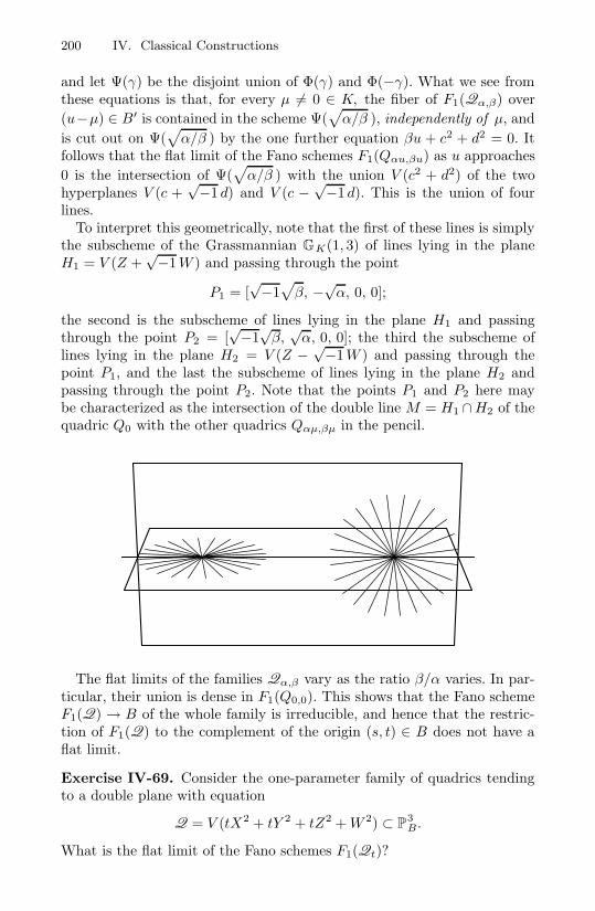
200 IV. Classical Constructions
and let Ψ(γ) be the disjoint union of Φ(γ) and Φ(−γ). What we see fromthese equations is that, for every µ = 0 ∈ K, the fiber of F1(Qα,β) over(u−µ) ∈ B′ is contained in the scheme Ψ(
√α/β ), independently of µ, and
is cut out on Ψ(√
α/β ) by the one further equation βu + c2 + d2 = 0. Itfollows that the flat limit of the Fano schemes F1(Qαu,βu) as u approaches0 is the intersection of Ψ(
√α/β ) with the union V (c2 + d2) of the two
hyperplanes V (c +√−1 d) and V (c − √−1 d). This is the union of four
lines.To interpret this geometrically, note that the first of these lines is simply
the subscheme of the Grassmannian GK(1, 3) of lines lying in the planeH1 = V (Z +
√−1W ) and passing through the point
P1 = [√−1
√β, −√
α, 0, 0];
the second is the subscheme of lines lying in the plane H1 and passingthrough the point P2 = [
√−1√
β,√
α, 0, 0]; the third the subscheme oflines lying in the plane H2 = V (Z − √−1W ) and passing through thepoint P1, and the last the subscheme of lines lying in the plane H2 andpassing through the point P2. Note that the points P1 and P2 here maybe characterized as the intersection of the double line M = H1 ∩H2 of thequadric Q0 with the other quadrics Qαµ,βµ in the pencil.
The flat limits of the families Qα,β vary as the ratio β/α varies. In par-ticular, their union is dense in F1(Q0,0). This shows that the Fano schemeF1(Q) → B of the whole family is irreducible, and hence that the restric-tion of F1(Q) to the complement of the origin (s, t) ∈ B does not have aflat limit.
Exercise IV-69. Consider the one-parameter family of quadrics tendingto a double plane with equation
Q = V (tX2 + tY 2 + tZ2 + W 2) ⊂ P3B.
What is the flat limit of the Fano schemes F1(Qt)?

IV.3 Fano schemes 201
More Examples. To see how the Fano scheme of lines on a quadric overa non-algebraically closed field may behave, we consider the example ofquadrics over the real numbers:
Exercise IV-70. Consider the quadrics Q1, Q2 and Q3 in P3R given by
the equationsQ1 = V (X2 + Y 2 − Z2 − W 2),
Q2 = V (X2 + Y 2 + Z2 − W 2),
Q3 = V (X2 + Y 2 + Z2 + W 2).
Show that the Fano scheme F1(Q1) is the union of two copies of P1R , while
the Fano scheme of lines on Q2 is irreducible but not absolutely irreducible.Finally, show that the Fano scheme F1(Q3) is the union of two copies of aplane conic not isomorphic to P1
R .
Here’s an example over a function field:
Exercise IV-71. Let B = P9K be the projective space that parametrizes
quadric surfaces in P3K , and L its function field. Let QB ⊂ P3
B be theuniversal quadric surface over B. Let QL ⊂ P3
L be the fiber of Q over thegeneric point Spec L of B, and FL = F1(QL) ⊂ GL(1, 3) its Fano scheme oflines. Describe FL. In particular, show that it behaves differently from theexamples above, in that is isomorphic to two copies of P1
M over a quarticextension M of L, but not over any quadratic extension of L. (In fact, thereis a quadratic extension L′ of L over which FL becomes reducible, but thecomponents of FL×LSpec L′ are forms of P1
L′ (in the sense of Section IV.4),but not isomorphic to P1
L′ .)
Finally, here is an arithemetic analogue:
Exercise IV-72. Consider the quadrics Q1, Q2 and Q3 ⊂ P3Z given by
Q1 = V (7X2 + 7Y 2 + Z2 + W 2)
Q2 = V (7X2 + 14Y 2 + Z2 + W 2)
Q3 = V (7X2 + 49Y 2 + Z2 + W 2).
Describe the Fano scheme F1(Qi) ⊂ GZ(1, 3) in each case. In particular,describe the component of F1(Qi) dominating Spec Z, and its intersectionwith the fiber GZ/(7)(1, 3) of GZ(1, 3) over the point (7) ∈ Spec Z.
IV.3.3 Lines on Cubic Surfaces
In the following series of exercises, we will develop some interesting factsabout the Fano scheme F1(S) parametrizing the lines on a cubic surface S ⊂P3
K . To begin with, the following two exercises establish that all nonsingularcubics contain the same number of lines (without deriving the number 27).

202 IV. Classical Constructions
Exercise IV-73. Let K be a field, S ⊂ P3K a nonsingular cubic surface,
and F = F1(S) ⊂ GK(1, 3) the Fano scheme of lines on S. Show that F isreduced.Hint : Take L ∈ F1(S) the line given by X = Y = 0, and write the cubicpolynomial defining S as X Q(Z, W ) + Y P (Z, W ) modulo (X, Y )2; showthat the condition that the tangent space T[L]F1(S) be positive-dimensionalis that P and Q have a common zero along L. (Compare this to the dis-cussion in Section VI.2.3.)
Exercise IV-74. Let P19K be the projective space parametrizing cubic sur-
faces in P3K , and U ⊂ P19
K the open subset corresponding to cubics hav-ing only finitely many lines (that is, other than cones and scrolls). LetSU ⊂ P3
U be the universal cubic in projective 3-space over U, and FU =F1(SU ) ⊂ GU (1, 3) be its Fano scheme of lines. Show that the projectionmap π : FU → U is flat.
Hint: Use the fact that the Fano scheme F1(S) of lines on a cubic surfaceS ⊂ P3
K is a local complete intersection, together with Proposition II-32.
In fact, neither of the statements of the two preceding exercises is com-pletely general: that is, for some d and n the Fano variety F1(X) of lines ona hypersurface X ⊂ Pn
K of degree d may be singular and even nonreducedfor X nonsingular; and the dimension dimF1(X) may jump as X varies,so that the universal Fano scheme F need not be flat. We will be able toexhibit examples of these behaviors once we have developed a descriptionof tangent spaces to Fano schemes in Chapter VI.
We now consider what happens when our cubic surface becomes singular.There are essentially two cases to consider. In some sense the simpler caseis when S has only isolated double points: in this case (as we will see)the Fano scheme F1(S) is still 0-dimensional of degree 27, and fits into aflat family with the Fano schemes of nonsingular cubics (that is, in termsof Exercise IV-74 above, if we let U ′ ⊂ P19
K be the larger open subset ofcubics having at most isolated double points as singularities, and defineSU ′ ⊂ P3
U ′ and FU ′ ⊂ GU ′(1, 3) accordingly, then FU ′ → U ′ is still flat).On the other hand, when S is a cone or has positive-dimensional singularlocus— for example, when S is reducible —F1(S) will become positive-dimensional; and a further question arises: what may be the flat limit ofthe Fano schemes F1(Sλ) ⊂ G(1, 3) as Sλ approaches S?
We start with some examples of cubic surfaces having isolated doublepoints. For this it may be useful to recall the description of such surfacesin Exercise IV-62 above, or in Griffiths and Harris [1978].
Exercise IV-75. Let K be an algebraically closed field, and S ⊂ P3K a
cubic surface having an ordinary double point P (that is, the projectivizedtangent cone to S at P is a nonsingular conic). Show that the Fano schemeF1(S) consists of six nonreduced points (each of multiplicity 2) correspond-ing to lines on S through P, and 15 reduced points.

IV.3 Fano schemes 203
Exercise IV-76. Now suppose that S has two ordinary double points Pand Q. Show that the scheme F1(S) consists of one point of multiplicity 4,supported at the point [PQ] corresponding to the line PQ joining P and Q;eight points of multiplicity 2 corresponding to lines through P or Q otherthan PQ; and 7 reduced points. What is the scheme structure of the point[PQ]?
Exercise IV-77. Now say that S has again just one double point P ;but suppose now that P is what is called an A2 singularity: that is, thecompletion of the local ring OS,P with respect to the maximal ideal isOS,P
∼= K[[x, y, z]]/(xy − z3) (in particular, the tangent cone is a conicof rank 2, as in Exercise IV-63). Show that the scheme F1(S) consists ofsix points of multiplicity 3, corresponding to lines on S through P, and9 reduced points. Again, what is the scheme structure of the points ofmultiplicity 3?
In case S is reducible or a cone, the Fano scheme of lines on S is usuallypretty obvious; what is of interest is, as we said, the flat limits of the Fanoschemes of nearby nonsingular cubics. We consider, in each of the followingproblems, the same set-up: we take S0 a reducible cubic or a cone, chooseS a general cubic, and let Sλλ∈P1 be the pencil of cubic surfaces thatthey span. In each case, we ask what will be the flat limit, as λ tends to 0,of the Fano schemes F1(Sλ).
Exercise IV-78. Take S0 the union of a nonsingular quadric Q and aplane H, meeting along a nonsingular conic curve C. Let P1, . . . , P6 =C∩S be the base points of the pencil lying on C. Show that the flat limit, asλ tends to 0, of the Fano schemes F1(Sλ) is reduced of degree 27, consistingof the 12 lines on Q containing one of the points Pi and the 15 lines on Hcontaining 2 of the points Pi.
Exercise IV-79. Now take S0 the union of three planes H1, H2, H3 ingeneral position. Again, what is the flat limit, as λ tends to 0, of the Fanoschemes F1(Sλ)?
Exercise IV-80. The same problem, but now take S0 the cone over anonsingular plane cubic curve.
Finally, an amusing one on the line(s) on the universal cubic:
Exercise IV-81. Let B = P19K be the projective space parametrizing cubic
surfaces in P3K , L the function field of B, SB ⊂ P3
B the universal cubic inprojective 3-space over K, and SL the fiber of S over the generic pointSpec L of B. Let FL = F1(SL) ⊂ GL(1, 3) be its Fano scheme of lines.Show that FL consists of one reduced point, whose residue field is a degree27 extension of L.
Hint: this follows from the fact that the universal Fano variety F =F1(S ) ⊂ GB(1, 3) = P19
K ×K GK(1, 3) is irreducible, which in turn follows

204 IV. Classical Constructions
from the fact that projection on the second factor expresses F as a P15K -
bundle over GK(1, 3).
Exercise IV-82. Consider now nonsingular cubic surfaces S ⊂ P3R over
the real numbers. As we have seen, the Fano scheme F1(SC) ⊂ GC(1, 3)of SC = S ×SpecR Spec C consists of 27 reduced points. It follows that,for some pair of integers a and b with a + 2b = 27, F1(S) ⊂ GR(1, 3) willconsist of a reduced points with residue field R and b reduced points withresidue field C. Show that a can be 3, 7, 15 or 27, and that no other valuesare possible. (See Segre [1942].)
IV.4 Forms
Let S be any scheme and X any scheme over S. We say that a scheme Y overS is a form of X if for every point p ∈ S there exists an open neighborhoodU of p in S and a flat surjective morphism T → U of schemes such thatY ×S T ∼= X ×S T as T -schemes.
To begin with a classic example, consider the conic in the real projectiveplane P2
R given by the equation X2 + Y 2 + Z2 = 0, that is, the curveC = ProjR[X, Y, Z]/(X2+Y 2+Z2). The curve C has no points defined overR—that is, no points with residue field R—and so cannot be isomorphic tothe projective line P1
R . However, the result of extending the ground field tothe algebraic closure C of R is C ×SpecR Spec C ∼= ProjC[X, Y, Z]/(X2 +Y 2 + Z2) ∼= P1
C . Thus C is a form of P1R over Spec R, or, more succinctly,
an R-form of the projective line.As a second example, the reader might check that the field extension
Spec Q[x]/(x2 + 1) over Spec Q is a form of the scheme consisting of twodistinct points, while Spec Z/(2)[x]/(x2 + 1) over Spec Z/(2) is a form of adouble point.
In number theory it is of interest to see how the set of rational pointsmay vary in a family of forms of a given curve. To give a particular case,for any t ∈ Q the set of rational solutions (x, y) of what is called Pell’sequation,
ty2 = x2 − 1,
is the set of Q-rational points on the curve Ct = Spec Q[x, y]/(ty2−x2+1).These curves Ct are forms of P1 over Spec Q. Likewise, the curves Et =Spec Q[x, y]/(ty2 − x3 + 1) all have j-invariant 0, and thus are all formsof the curve E1 ⊂ P2
Q given by y2 = x3 − 1 (see Section IV.2.3 above andSection VI.2.4 below), but have varying arithmetic properties.
In each of these cases, it is easy to see that the curves given are forms ofeach other—the curves Et ×Spec Q Spec Q[
√t] and E1 ×SpecQ Spec Q[
√t]
are visibly isomorphic—and less obvious but not hard to see that they arenot all isomorphic. (In fact the naive guess—that Et
∼= E1 if and only if
IV.4 Forms 205
t ∈ (Q∗)2, that is, t is the square of a nonzero rational number—is correct,but it is a nontrivial exercise to prove this.)
The set of isomorphism classes of S-forms of projective space Pn, for alln, is in a natural way a group, called the Brauer group of S (or, in caseS = Spec K is the spectrum of a field, the Brauer group of K), with the trueprojective space Pn
S the identity element. This group may be computed withGalois cohomology; see Serre [1975]. Here is a construction of the Brauergroup related to number theory:
Let K be a field, and let A be an n-dimensional Azumaya algebra overK—that is, A is an algebra which has dimension n as a vector space, hasno nontrivial 2-sided ideals, and has center exactly K. For example, thealgebra Md(K) consisting of all d × d matrices over K is a d2-dimensionalAzumaya algebra. It follows from the Wedderburn structure theorems thatif A is an n-dimensional Azumaya algebra over K then n is a square, sayn = d2, and K ⊗ A ∼= Md(K) ∼= K ⊗ Md(K) (in this sense A is a form ofMd(K).)
Identifying Md(K) with the endomorphism algebra of a d-dimensionalvector space V over K, it is easy to see that the left ideals of Md(K) eachhave the form
a ∈ Md(K) | Im(a) ⊂ W
for some subspace W ⊂ V. The vector space dimension of the left ideal isthen dim(V ) dim(W ). In particular, the left ideals of dimension equal tod(d − 1) correspond to the hyperplanes in V, that is, the points of P(V ).The subscheme of the Grassmannian of d(d− 1)-planes in Md(K) that areclosed under multiplication by Md(K)— that is, are ideals — is isomorphicto Pd(K) in this way.
At the other extreme, there are (in general) Azumaya algebras A that aredivision algebras over K — that is, algebras with no left ideals at all. Butwe can still form the scheme of left ideals of A. Of course we must specifyit by equations, not as a point set! Let G be the Grassmannian of d(d− 1)-dimensional subspaces of the vector space A. If S ⊂ AG is the universalbundle then the subscheme of G that we want is the largest subscheme Xsuch that the restriction to X of the composite map of vector bundles
S ⊗ AG ⊂ AG ⊗ AGmultiplication A A/S
on G is zero (this is locally a subscheme defined by the d(d−1)d2×d entriesin a matrix representing the composite map.) Extending the ground field,we find that XK is the Grassmannian of d(d−1) dimensional ideals of K⊗A,that is, projective space! Conversely, it can be shown that every form ofprojective space over K occurs in this way and that the correspondencebetween isomorphism classes of forms and Azumaya algebras is one-to-one.For all this see Serre [1975] and Cassels and Frohlich [1967].

206 IV. Classical Constructions
Exercise IV-83. Let A be the quaternion algebra over R; that is, thealgebra with basis 1, i, j, k and multiplication i2 = j2 = k2 = −1, ij =−ji = k. Check that its center is R, and that it is a division algebra (andthus an Azumaya algebra over R). Compute the equations of the schemeof 2-dimensional left ideals of A in terms of Plucker coordinates on theGrassmannian of lines in P(A) ∼= P3
R . Show directly that this is a form ofP1.
Here is still another way in which a form of P1 arises, on which thereader can try his hand: Let K be an algebraically closed field, and letB = P5
K be the projective space parametrizing conic curves in P2K . Let
U ⊂ B be the open subset corresponding to nonsingular plane conics, andlet CU ⊂ P2
U = U ×SpecK P2K be restriction to U of the universal conic
curve C ⊂ P2B over B as described in Section III.2.8. Similarly, let L be
the function field of B (or equivalently of U), Spec L the generic point ofB, and CL ⊂ P2
L the fiber of the universal conic C over Spec L. We have:
Proposition IV-84. CU is a nontrivial form of P1U over U and CL a
nontrivial form of P1L over L.
The point is that, although every smooth conic plane curve in P2K is
rational, there is no way of choosing a rational parametrization of eachsmooth conic consistently over a Zariski open subset of U.
Proof. To establish our claims, it will be enough to show two things: thatCU is a form of P1 over U, and that CL ∼= P1
L. To see the first, fix a lineM ⊂ P2
K and let
V = CU \ (CU ∩ (U × M)) ⊂ U × P2K .
We claim that the pullback
CV = V ×U CU ⊂ U × P2K × P2
K
is isomorphic to the product V ×M ∼= P1V as V -schemes. The point is, the
family CV → V has naturally a section—the diagonal—and the presenceof a distinguished point on each fiber of CV → V allows us parametrizethat fiber by projecting from that point onto M. Explicitly, away from thediagonal in CV we can define a map ϕ : CV → V × M by
ϕ : (C, p ; q) −→ (C, p ; p, q ∩ M .
Exercise IV-85. Show that
(a) ϕ is a morphism of schemes;
(b) ϕ extends to a morphism on all of CV (sending a point (C, p, p) on thediagonal in CV to the point of intersection with M of the tangent lineat p to the fiber of CV over (C, p) ∈ V );
(c) ϕ : CV → V × M is an isomorphism.

IV.4 Forms 207
For the second part, observe that if CL were isomorphic to P1L, it would
have an L-rational point—that is, a pair of rational functions F (a, b, c, d, e)and G(a, b, c, d, e) ∈ K(a, b, c, d, e) such that
1 + aF 2 + bG2 + cF + dG + eFG = 0.
We can assume (after possibly a change of variables on our original P2K)
that the denominators of F and G are not in the ideal (c, d, e); so thatrestricting to the locus c = d = e = 0 we get four polynomials f(a, b),g(a, b), h(a, b) and j(a, b) such that
1 + a ·(
f(a, b)h(a, b)
)2
+ b ·(
g(a, b)j(a, b)
)2
= 0;
or, in other words,
h(a, b)2j(a, b)2 + a · f(a, b)2j(a, b)2 + b · g(a, b)2h(a, b)2 = 0.
Now we simply ask what the degree of each term in this equation is, firstas a polynomial in a and then in b, and thus derive a contradiction.
Exercise IV-86. Let K be any field. Show that any form X of P1K over
Spec K is isomorphic to a plane conic C ⊂ P2K . Conclude in particular that
a form X of P1K over Spec K is isomorphic to P1
K if any only if it has apoint with residue field K.
Exercise IV-87. Using the preceding exercise, show that a form X of P1K
over a field K is isomorphic to P1K if any only if it has a zero-dimensional
subscheme Γ ⊂ X of odd degree, that is, such that the coordinate ring ofΓ has odd dimension as a vector space over K.
Exercise IV-88. Show that there are no nontrivial forms of A1K over
Spec K, that is, any form of A1K over Spec K is isomorphic to A1
K .
Exercise IV-89. Show by example that the conclusions of the three pre-ceding exercises are all false if we do not specify S = Spec K, that is, if weconsider forms X of P1
S and A1S over a general scheme S. (To find coun-
terexamples, it is enough to take S = P1K a projective line over a field and
consider the blow-up of the affine plane A2K at the origin.)
Another generalization of the irrationality of the universal conic —thistime asserting that the universal rational normal curve of degree d is ratio-nal if and only if d is odd— will be discussed in Exercise VI-38.
For another example of a form of projective space arising in a geometriccontext, see Exercise IV-71 above.

VLocal Constructions
V.1 Images
In this section we will be concerned with a basic notion: the image of amorphism in the category of schemes. As we will see, there are two fun-damental properties that we would like the notion of image to have, thepush-pull property and invariance under base change; but the two are in-compatible. We will give accordingly two definitions, one straightforwardand one less so, each of which is useful in certain situations.
V.1.1 The Image of a Morphism of Schemes
Suppose ϕ : X → Y is a morphism of schemes. The set-theoretic image ofϕ is defined in the obvious way: it is the subset of Y consisting of thosepoints y ∈ Y such that there is a point x ∈ X with ϕ(x) = y. The imagemay or may not be a closed subset: for example, if X is the scheme definedby the ideal (xy − 1) ⊂ K[x, y] in A2
K = Spec K[x, y], then the image ofthe projection of X to the affine line A1
K = Spec K[x] is the complementof the origin, an open set. In a certain sense this is because we “forgot”some of the points of the source scheme: if we extend this morphism toa morphism from the closure of X in A1
K ×K P1K , the image becomes the
whole projective line.These two examples turn out to be typical. The situation is summed up
in the following theorem. To state it, recall that a subset V of a topologicalspace is constructible if it is a finite union of locally closed subsets Vi.

210 V. Local Constructions
Theorem V-1. If the morphism of Noetherian schemes ϕ : X → Y isof finite type, the set-theoretic image of ϕ is constructible in Y. If themorphism ϕ is projective, the set-theoretic image of ϕ is closed.
The first of these statements is due to Chevalley. Note the necessity ofthe hypothesis that ϕ is of finite type: the morphism
Spec K[x1, . . . , xn](x1,...,xn) −→ Spec K[x1, . . . , xn],
coming from the inclusion of the polynomial ring in its localization, doesnot have constructible image for any n. The second statement, which isquite old, is generally called the Main Theorem of Elimination Theory. Thedefinition of properness, which is a strengthening of the conclusion of thetheorem, was essentially made to express this property (see Section III.1).The proof of Theorem V-1 is exactly the same as in the classical case ofvarieties; see for example Harris [1995] or Hartshorne [1977]. We will notrepeat it here.
More novel is the fact that the closure of the image has a natural schemestructure, and this is the fact that we shall explore in this section.
Suppose now we wish to define the image of a morphism ϕ : X → Yas a scheme. What we would like ideally— though, as we shall see, thisis impossible— is to take ϕ(X) to be the smallest subscheme of Y whoseinverse image is all of X. In other words, we would characterize ϕ(X) bythe push-pull property: for every subscheme Z ⊂ Y,
Z ⊃ ϕ(X) ⇐⇒ ϕ−1(Z) = X.
As it happens, though, no such subscheme of Y need exist, as shown bythe example of the morphism
ϕ : X = A2K −→ Y = A2
K
defined by the ring homomorphism ϕ# : K[x, y] → K[s, t] taking x to sand y to st.

V.1 Images 211
For any λ ∈ K, let Yλ be the complement in Y of the point (0, λ). Forλ = 0, the inverse image of Yλ is all of X . Thus, if there were a subschemeϕ(X) ⊂ Y satisfying the push-pull property above with Z = Y , the supportof ϕ(X) would be contained in the set I =
⋂λ=0 Yλ, which is the union of
the point (0, 0) and the complement of the x-axis. On the other hand, fromϕ−1ϕ(X) = X it would follow that the support of ϕ(X) contained I, andhence that suppϕ(X) = I. But I is not a locally closed subset of Y , andso is not the support of any subscheme of Y .
We are, however, close to what we want: there does exist a smallest closedsubscheme of Y whose inverse image is all of X, and this subscheme doessatisfy the push-pull property with respect to closed subschemes Z ⊂ Y.
Definition V-2. If ϕ : X → Y is a morphism of finite type, then thescheme-theoretic image, written ϕ(X), is the closed subscheme of Y whosesheaf of ideals is the sheaf of regular functions on open subsets of Y thatpull back to 0 under ϕ#, that is,
ϕ(X) = V(Ker(ϕ# : OY → ϕ∗OX)
) ⊂ Y.
We say that ϕ is dominant if ϕ(X) = Y, or equivalently if the pullbackmap ϕ# is a monomorphism.
This condition that a morphism be dominant is not just a conditionon the underlying map of topological spaces: for example, the inclusionϕ : Spec K → Spec K[ε]/(ε2) is a surjection on underlying sets, but theimage is a proper closed subscheme, the pullback map ϕ# is not injective,and the map is not dominant.
Proposition V-3. If ϕ : X → Y is a morphism of schemes, the closureof the set-theoretic image is ϕ(x)red.
Proof. We may reduce at once to the affine case, and prove that if ϕ# :B → A is a ring homomorphism then the intersection J of all the primes Qof B that may be written in the form Q = (ϕ#)−1(P ) for some prime P ofA is the radical of Ker(ϕ#) (see Section I.2.1). Let I ⊂ A be the nilradicalof A. We have
J =⋂
P⊂A prime
(ϕ#)−1(P ) = (ϕ#)−1(I).
Thus if f ∈ J then ϕ#(f) ∈ I is nilpotent, and f ∈ rad(Ker ϕ#). Theopposite inequality is immediate.
It is sometimes convenient to work in an apparently more general case:If ϕ : X → Y is any morphism and X ′ ⊂ X a closed subscheme, then wedefine the scheme-theoretic image ϕ(X ′) of X ′ to be the subscheme definedby the sheaf of ideals I with
I(U) = f ∈ OY (U) | ϕ#(f) ∈ IX′(ϕ−1(U).

212 V. Local Constructions
This “generalization” actually describes a special case, since ϕ(X ′) is thescheme-theoretic image of the composite morphism X ′ → X → Y.
If the two schemes X and Y are affine and the map ϕ is dominant, thenthe ideal describing the image of a subscheme X ′ ⊂ X is obtained in aparticularly simple way: we may think of A(Y ) as a subring of A(X), andϕ(X ′) is the subscheme of Y defined by IX′ ∩ A(Y ). We shall be mostlyconcerned with this case, since it already contains all the new phenomena.
As an example consider the linear projection on the first coordinate
ϕ : X = A2K = Spec K[x, y] −→ Y = A1
K = Spec K[x]
Let X ′ and X ′′ be the (abstractly isomorphic) zero-dimensional subschemesgiven by the ideals I ′ = (x, y2) and I ′′ = (x2, y). The image of X ′ is thereduced scheme defined by (x, y2) ∩ K[x] = (x), while the image of X ′′ isgiven by (x2, y)∩K[x] = (x2). More generally, the image of the “fat point”V (x2, xy, y2) ⊂ A2
K is the double point V (x2) ⊂ A1K ; and the image of the
double point V (x2, xy, y2, αx+βy) ⊂ A2K is the double point V (x2) ⊂ A1
K
for β = 0, but the reduced point V (x) for [α, β] = [1, 0].We see from thisexample that the scheme structure of the image depends on the relation ofthe subscheme to the fibers of the morphism ϕ.
Exercise V-4. Consider now a “family” of such projections of doublepoints: take B = Spec K[t] = A1
K and consider the morphism
ϕ : X = A2B = Spec K[x, y, t] −→ Y = A1
B = Spec K[x, t].
Let X ′ ⊂ X be the double line
X ′ = V (x2, xy, y2, x+ty) ⊂ A2B
as described in Section II.3.5. Show that the scheme-theoretic image ϕ(X)of X ′ is the double line V (x2) ⊂ Y, even though the fiber of X ′ over theorigin (t) ∈ B has image the reduced point V (x) in the fiber of Y over(t). This is in fact the source of some interesting complications, as we willexplain in the following section.

V.1 Images 213
Exercise V-5. Show that if ϕ : X → Y is a morphism and X ′ ⊂ X is areduced subscheme, then ϕ(X ′) is reduced. (Hint: Reduce to the statementthat the preimage of a radical ideal under a ring homomomorphism is againradical.)
V.1.2 Universal Formulas
Is there a “formula” for the closure of the image of a map, and if so, whatis it? This question, in a somewhat different language, occupied a largenumber of mathematicians in the past, and the theory is correspondinglyrich. In many special cases beautiful and useful formulas were found forthe set-theoretic image; the equations they give are usually referred to asresultants, a notion we will discuss below. The scheme-theoretic image issignificantly more complicated: with a reasonable interpretation of the basicquestion there can be no formula for the scheme theoretic image! We shallnext explain this fact and the opportunities to which it gives rise. We shallkeep the discussion informal, but it can be formalized using the notion offamily of schemes given in Section II.3.4.
Consider a consequence that a universal formula would have: it wouldbe preserved by base change, or, put more informally, it would specializeon substitution of variables. Some examples will make this clear.
Example V-6. (See figure on the next page.) To begin with, let K bean algebraically closed field, set B = Spec K[t] = A1
K , and consider theprojection map
ϕ : A2B = Spec K[t, x, y] → A1
B = Spec K[t, x]
defined by the inclusion K[t, x] ⊂ K[t, x, y]. We regard this map infor-mally as a (trivial) family of projection maps A2
K = Spec K[x, y] → A1K =
Spec K[x] parametrized by t ∈ K. Consider first the closed subschemeX ⊂ A2
B = A3K given as the union of the two disjoint lines V (y, x) and
V (y−1, x+ t); that is,
X = V (y2−y, yx+yt, yx−x, x2 + tx).
We will think of X as a family of pairs of points in the (x, y)-plane, param-etrized by t, and each with its projection onto the x-axis: for each scalara ∈ K we let Xa ⊂ A2
K be the fiber of X over the point (t − a) ∈ B,Ya
∼= A1K the fiber of A1
B over (t − a) and ϕa : Xa → Ya the restriction ofϕ to Xa.
For each scalar value a = 0 ∈ K the set-theoretic image ϕ(Xa) is theunion of the two points x = 0 and x = −a; for a = 0 it is simply the originx = 0. The scheme-theoretic image ϕ(Xa) is the subscheme of Spec K[x]defined by the ideal Ia := K[x]∩(y2−y, yx+ay, yx−x, x2 +ax). Since
K[x, y]/(y2−y, yx+ay, yx−x, x2 +ax) = K[x, y]/(y2−y, x+ay),

214 V. Local Constructions
XaX0
ϕ(Xa) = ϕ(X)a
ϕ(X0) = ϕ(X)0
we see that
Ia = Ker(K[x] → K[x, y]/(y2 − y, x + ay)
)=
(x2 + ax) if a = 0,(x) if a = 0.
Thus the scheme-theoretic image ϕ(Xa) is the union of two reduced pointsfor a = 0 and a single reduced point for a = 0.
The important thing about this example is that the scheme-theoreticimages ϕ(Xa) do not fit into any family of schemes! That is, there is nopolynomial f(t, x) “giving a formula for the scheme-theoretic image” in thesense that for each a ∈ K the scheme-theoretic image ϕ(Xa) is defined bythe ideal f(a, x) = 0. Indeed, for a = 0 the scheme ϕ(Xa) is defined bythe ideal (x2 + ax), so we would have to have f(t, x) = g(t, x)(x2 + tx) forsome polynomial g(t, x). Since g(a, x) = 0 for all x when a = 0, we musthave g(t, x) = g(t), a polynomial of one variable vanishing at most whent = 0. If now g(0) = 0 then f(0, a) would describe the whole line, while ifg(0) = 0 then f(0, a) would describe a double point, and neither of theseoptions is the scheme-theoretic image ϕ(Xa).
Perhaps the best we can do in this example is to take the scheme-theoreticimage of the whole family, ϕ(X) ⊂ Spec K[x, t]. This image is defined bythe ideal K[t, x]∩(y2−y, yx+yt, yx−x, x2 + tx). To compute this inter-section, one shows that the localization map
K[t, x, y]/(y2 − y, yx + yt, yx − x, x2 + tx)→ K[t, t−1, x, y]/(y2 − y, yx + yt, yx − x, x2 + tx)
= K[t, t−1, x]/(x2 + tx)
is a monomorphism, and it follows at once that the intersection is (x2 +tx).

V.1 Images 215
We thus see that the scheme-theoretic image ϕ(X0) of the fiber of Xover the origin (t) ∈ B is properly contained in the fiber ϕ(X)0 of thescheme-theoretic image ϕ(X) over the origin. In particular, the fiber of anyclosed subscheme of A1
B containing ϕ(Xa) for a = 0 will properly containϕ(X0), so that the scheme-theoretic images ϕ(Xa) cannot form a family inany sense. The equation x2 + tx of the scheme-theoretic image ϕ(X) givesthe “correct” defining ideal for ϕ(Xa) when we specialize t to any a = 0,while for a = 0 it gives an ideal defining a scheme a little larger than ϕ(X0).This choice of “approximation” for a defining equation of scheme-theoreticimages is a resultant, in a sense that we shall describe.
Example V-7. (See figure below.) To see an example of the same phe-nomenon involving nonreduced schemes, let K, B = Spec K[t] = A1
K , and
ϕ : A2B = Spec K[t, x, y] → A1
B = Spec K[t, x]
be as before, and consider the closed subscheme X ⊂ A2B = A3
K given by
X = V (x2, xy, y2)∩V (ty+x) = V (ty+x, y2).
Viewed as a subscheme of A2B = A3
K , it is the intersection of the firstorder infinitesimal neighborhood of the t-axis with a helical surface windingaround the axis; it is a double line supported on the t-axis. As before, wewill think of X as a family of double points in the plane, each with itsprojection onto the y-axis: for each scalar a ∈ K we let Xa ⊂ A2
K be thefiber of X over the point (t− a) ∈ B, Ya
∼= A1K the fiber of A1
B over (t− a)and ϕa : Xa → Ya the restriction of ϕ to Xa.
ϕ(Xa) = ϕ(X)a
ϕ(X0) = ϕ(X)0
X0
Xa

216 V. Local Constructions
For each scalar value t = a ∈ K the set-theoretic image ϕ(Xa) is thepoint x = 0. The scheme-theoretic image ϕ(Xa) is defined by Ia := K[x]∩(ay + x, y2). Since
K[x, y]/(ay + x, y2) =
K[x]/(x2) if a = 0,K[x, y]/(x, y2) if a = 0,
we see that
Ia = Ker(K[x] → K[x, y]/(ay+x, y2)
)=
(x2) if a = 0,(x) if a = 0.
Thus the scheme-theoretic image ϕ(Xa) is a double point for a = 0 and asimple point for a = 0.
Just as in the previous example, we see that the scheme-theoretic imagesϕ(Xa) cannot be the fibers of any closed subscheme of A1
B over B. In partic-ular, the scheme-theoretic image of the whole family, ϕ(X) ⊂ Spec K[x, t]is defined by the ideal K[t, x]∩(ty+x, y2), which is readily seen to be simply(x2) (as before, this follows from the fact that the localization map
K[t, x, y]/(ty+x, y2) → K[t, t−1, x, y]/(ty+x, y2) = K[t, t−1, x]/(x2)
is a monomorphism). We thus see that the scheme-theoretic image ϕ(X0)of the fiber of X over the origin (t) ∈ B is properly contained in thefiber ϕ(X)0 of the scheme-theoretic image ϕ(X) over the origin, so thatthe fiber of any closed subscheme of A1
B containing ϕ(Xa) for a = 0 willproperly contain ϕ(X0). Once again it follows that the scheme-theoreticimages ϕ(Xa) cannot form a family of schemes.
Note also that as before the equation x2 of the scheme-theoretic imageϕ(X) gives the “correct” defining ideal for ϕ(Xa) for every a = 0, while fora = 0 it gives an ideal defining a scheme a little larger than ϕ(X0); again,the equation x2 of the fiber ϕ(X)a is an example of a resultant.
We may generalize the phenomena that we have just seen by saying thatfor any family of morphisms
Xϕ Y
B
with parameter space B and closed point b ∈ B, we have an inclusion
ϕ(Xb) ⊂ ϕ(X)b,
but this inclusion need not be an equality: in other words, the fiber ofthe image may properly contain the image of the fiber. This is sometimesexpressed by saying that the scheme-theoretic image does not necessarilycommute with base change. (The base change in question is pullback viathe inclusion b → B, though the same issues arise for any morphism

V.1 Images 217
B′ → B.) Note by contrast that the set-theoretic image does commutewith base change; this is just set-theory. A still more general form of thisstatement is expressed by the following result:
Proposition V-8. If
X ′ = X×Y Y ′ ψ′ X
Y ′
ϕ′
ψ Y
ϕ
is a pull-back diagram of morphisms of schemes, then ϕ′(X ′) ⊂ ψ−1ϕ(X).If the morphism ϕ is finite, these two schemes have the same underlyingset, the closure ϕ′(X ′) of the set theoretic image. In particular, when ϕ isfinite the set-theoretic image is closed. If ψ is flat, then ϕ′(X ′) = ψ−1ϕ(X).
Note that, in the previous case, Y ′ = Yb was the fiber of a morphismY → B, but we need not assume that in general.
Proof. We reduce at once to the affine case, and consider this diagram ofcoordinate rings:
A′ = A⊗BB′ ψ′#A
B′
ϕ′#
ψ#
B
ϕ#
In this setting the first assertion becomes the inequality
Ker(ϕ′#) ⊃ ψ#(Ker(ϕ#))B′,
which is immediate from the commutativity of the diagram.The second statement of the proposition becomes in this affine case the
assertion that, if A is a finite B-module, then the radicals of the ide-als Ker(ϕ′#) and ψ#(Ker(ϕ#))B′ are equal. Given the inequality above,and the fact that the radical of an ideal is the intersection of the primescontaining it, we must show that if P ′ is a prime ideal of B′ containingψ#(Ker(ϕ#))B′ then P ′ ⊃ Ker(ϕ′#).
The preimage P = (ψ#)−1P ′ of P ′ in B contains Ker(ϕ#), so we haveA⊗BBP = 0. Since A is a finitely generated B-module, Nakayama’s LemmaEisenbud [1995, Section 4.1] shows that A ⊗B BP /PP = 0. Since the unitelement of B maps to the unit element of A and BP /PP is a field, we seethat the induced map BP /PP → A ⊗B BP /PP is a monomorphism. Now

218 V. Local Constructions
consider the diagram
(A ⊗B B′) ⊗ B′P ′/P ′
P ′ = A ⊗B BP /PP ⊗BP /PPB′
P ′/P ′P ′ A ⊗B BP /PP
B′P ′/P ′
P ′
BP /PP
obtained by localizing and factoring out P ′ and P. Since BP /PP is a fieldand the right-hand vertical arrow is a monomorphism, the left-hand verticalarrow is also a monomorphism (every module is flat over a field!). It followsthat the kernel of ϕ′# is contained in P ′ as required.
The closedness of the set-theoretic image of ϕ when ϕ is finite followsif we take Y ′ to be a point of Y in the closure of the set-theoretic image(and thus in the scheme- theoretic image) and pull back via the inclusionmorphism of this point.
For the last statement, suppose that ψ is flat, that is, B′ is a flat B-module. Tensoring B′ with the exact sequence
0 −→ Ker(ϕ#) −→ B −→ Im(ϕ#) −→ 0
and the inclusion Im(ϕ#) → A gives back an exact sequence and an inclu-sion; and we see in particular that (Ker(ϕ#))B′, which is the image of
B′ ⊗B Ker(ϕ) → B′ ⊗B B = B′
is the kernel of ϕ′, as required.
The second (“equality”) statement of the proposition fails in general, forexample in the fiber product diagram of affine schemes corresponding tothe diagram of rings
0 K(t)
K
0 ← tK[t]
However, the equality statement does hold whenever the map ϕ is projec-tive— the proof, which would take us too far afield, may be reduced againto Nakayama’s Lemma using the deep fact that, when ϕ is projective,ϕ∗(OX) is a finite OY -module; see Hartshorne [1977], Corollary II.5.20.
Despite the nonexistence of a universal formula for the scheme-theoreticimage, there are, as we have mentioned, many formulas giving equationsthat define it set-theoretically, and each of them gives a scheme containingthe scheme-theoretic image, as one sees from the previous proposition. Oneway to produce such a formula is to choose a universal model, a family ofmorphisms parametrized by a scheme B, say
X0ϕ0−→ Y0
π−→ B

V.1 Images 219
such that the morphisms we are interested in occur as pullbacks, say
X = (πϕ0)−1(b)ϕ−→ Y = π−1(b),
with morphism ϕ the restriction of ϕ0. We then take the actual scheme-theoretic image of ϕ0 and restrict it to Y. We call the defining equationsof the scheme-theoretic image of ϕ0 resultants. By Proposition V-8, theseequations define a scheme in Y containing the scheme-theoretic image, andin some cases, such as when ϕ0 is finite, they define a scheme that has theclosure of the set-theoretic image as underlying set.
It turns out that resultants are often conveniently described as determi-nants. Before coming to this, we explain a general context in which thesedeterminants arise.
V.1.3 Fitting Ideals and Fitting Images
There is, at least in a restricted context, an alternative notion of the imageof a morphism ϕ : X → Y of schemes, which we will call the Fitting imageand denote by ϕFitt(X). This has the virtue that it does commute withbase change, but the defect that (since, as we will see below, the Fittingimage ϕFitt(X) may properly contain the scheme-theoretic image ϕ(X)) itdoes not have the push-pull property.
Fitting Ideals. To set this up, we need the sheaf-theoretic version ofFitting’s lemma. Let X be a scheme, let F be a coherent sheaf on X, andlet
E1Ψ−→ E0 −→ F −→ 0
be an exact sequence with E0∼= On
X and E1∼= Om
X free sheaves. (Herewe allow m to be infinite.) For any integer l, we define the ideal of l × lminors of Ψ to be the sheaf Il(Ψ) ⊂ OX of ideals generated by the l × lminors of a matrix representative of Ψ. This is independent of the choiceof isomorphisms E0
∼= OnX and E1
∼= OmX , and can also be defined when
E1 and E0 are merely quasicoherent, since it can also be described as theimage of the natural map
l∧E1 ⊗
l∧E ∗
0 −→ OX
induced by Ψ. The key fact about the ideals Il(Ψ) is Fitting’s Lemma. SeeEisenbud [1995, page 497] for a proof.
Lemma V-9 (Fitting’s Lemma). If
EΨ−→ On
X −→ F −→ 0
and
E ′ Ψ′−→ On′X −→ F −→ 0

220 V. Local Constructions
are exact sequences, then for each k ∈ Z
In−k(ψ) = In′−k(ψ′).
In view of the lemma, we may make the following definition:
Definition V-10. The k-th Fitting ideal Fittk F of the sheaf F is theideal given locally as In−k(Ψ) for any presentation of F as above. Thezero locus V (Fittk F ) ⊂ X will be called the k-th Fitting scheme of F.
It is instructive to compare the geometry of the zeroth Fitting ideal withthe more naive notion of the support of a sheaf F. Briefly, for any coherentsheaf F on a scheme X we define the annihilator annF ⊂ OX by taking(annF )(U) ⊂ OX(U) to be the annihilator of F (U) as an OX(U)-modulefor each open set U ⊂ X. We define the support of F, denoted supp(F ),to be the zero locus V (annF ) ⊂ X of the annihilator as a subscheme of X.
(Note that “support” is used in two different senses: the support of ascheme is its underlying set or topological space, while the support of asheaf is a scheme. In those cases where we wish to refer to the underlyingset of the support of a sheaf F — that is, supp(supp F )— we will call itsimply the “set-theoretic support”.)
For any coherent sheaf F on a scheme X we have
(Fitt0 F ) · F = 0,
so that Fitt0 F ⊂ ann F . In the other direction, if F admits a presentation
OnX −→ F −→ 0
then Fitt0 F ⊃ (annF )n. See for example Eisenbud [1995, Proposition20.7] for both these inequalities. It follows from the first of these propertiesthat
V (Fitt0 F ) ⊃ suppF ,
that is, the zeroth Fitting scheme contains the support of F ; and from thesecond that the underlying sets of the subschemes V (Fitt0 F ) and suppFare equal, that is, ∣∣V (Fitt0 F )
∣∣ = |suppF | .The difference lies in the scheme structure: the zeroth Fitting ideal may
be properly contained in the annihilator of F, and the zeroth Fittingscheme correspondingly may properly contain the support of F.
For example, consider the scheme X = A1K = Spec K[x], with sub-
schemes Y = V (x) and Z = V (x2). The sheaves
F = OZ and G = OY ⊕ OY
each have length 2; but the support of F is Z, while the support of G isthe smaller scheme Y. By contrast, we see that the zeroth Fitting schemesare equal:
V (Fitt0 F ) = V (Fitt0 G ) = Z.

V.1 Images 221
Exercise V-11. (a) If X is any scheme, Y ⊂ X a subscheme, the zerothFitting ideal Fitt0 OY of the structure sheaf of Y is simply the idealsheaf IY of Y, and the 0th Fitting scheme correspondingly is Y itself.
(b) Show that the zeroth Fitting ideal of a direct sum is the product of thezeroth Fitting ideals of the summands, that is, for any pair of coherentsheaves F and G on X,
Fitt0(F ⊕ G ) = Fitt0 F · Fitt0 G .
Show by example that this is not true if F ⊕ G is replaced by anarbitrary extension of F by G, that is, a sheaf H such that thereexists an exact sequence
0 −→ F −→ H −→ G −→ 0.
(c) Deduce from the first two parts of this exercise that if X is a regularone-dimensional scheme (for example, X = A1
K or X = Spec Z) andF is any sheaf whose set-theoretic support is a closed point p ∈ X,then
Fitt0 F = mlp,
where l is the length of F.
Fitting Images. Suppose now that ϕ : X → Y is a finite morphism ofschemes. The direct image ϕ∗OX is then a coherent sheaf on Y, and by ourdefinition the scheme-theoretic image ϕ(X) is the support supp(ϕ∗(OX))of this sheaf. Taking the zeroth Fitting scheme instead of the support givesus the promised alternative definition of image that commutes with basechange:
Definition V-12. For any finite morphism ϕ : X → Y of schemes, theFitting image of ϕ is the zeroth Fitting scheme of the direct image ϕ∗(OX),that is,
ϕFitt(X) = V (Fitt0 ϕ∗(OX)).
For any closed subscheme Z ⊂ X, we will likewise define the Fitting imageϕFitt(Z) to be the Fitting image of ϕ restricted to Z, that is, the zerothFitting scheme of the direct image ϕ∗(OZ)
Exercise V-13. Consider Examples V-6 and V-7. In each case, show thatthe Fitting image of the fiber X0 of X over the origin is a double point,not a reduced point, so that we have
ϕFitt(X0) = ϕFitt(X)0.
Exercise V-14. Consider the projection and inclusion morphisms
X = Spec K[ε]/ε2ϕ−→ Spec K
ι−→ Spec K[t].
Show thatιFitt(ϕFitt(X)) (ι ϕ)Fitt(X).

222 V. Local Constructions
V.2 Resultants
V.2.1 Definition of the Resultant
The oldest— and still one of the most important— applications of the ideaswe have introduced in the last two subsections is the resultant of two poly-nomials in one variable. To define this, say we are given two polynomials
f(x) = a0xm + · · · + am,
g(x) = b0xn + · · · + bn,
with coefficients ai, bi in a field K. The goal was to describe the conditionon the coefficients ai, bi for the two polynomials to have a common factor;that is, a common root in the algebraic closure of K. In applications it isalso natural to look at families of polynomials. That is, we may take thecoefficients ai, bi to be regular functions on a base scheme B, so that wethink of f and g as “families of polynomials in one variable parametrizedby B”, and we wish to describe the locus in B over which f and g have acommon factor. More precisely, we want to describe the image in B —inwhichever sense!— of the scheme V (f, g) ⊂ A1
B.
There are, roughly speaking, four ways to interpret this problem: wecould ask formulas, in terms of the ai’s and bi’s, for functions generatingthe ideal of
(1) the reduced image of V (f, g)— that is, the reduced scheme associatedto the scheme-theoretic image;
(2) the scheme-theoretic image of V (f, g);
(3) the Fitting image of V (f, g); or
(4) the pullback of the image from a suitable universal family.
As shown by examples such as V-6 and V-7 above, no such formula canexist for the images in the first two senses. We shall begin by describingthe classical approach, and ultimately show that (for the correct choiceof “universal family”) it coincides with the third and fourth options, andcommutes with base change.
To carry out the classical approach, we begin by choosing a universalfamily. We will work not over a field but over an arbitrary ring S. Let Abe the polynomial ring
A = S[a0, . . . , am, b0 . . . , bn].
With f and g defined as above, we set
X := V (f, g) ⊂ A1A
and letϕ : X ⊂ A1
A = Spec A ×S A1S −→ Spec A =: Y.

V.2 Resultants 223
Since X is defined by two polynomials, we might expect it to have codi-mension 2 in A1
A. In this case, assuming that the map is “generically finite”(that is, finite over some open set) its image would have codimension 1 inSpec A. In the classical situation, where S is field, A has unique factoriza-tion, so the closure of the image would be described by one equation, calledthe resultant of f and g.
It turns out that the conclusion of this suggestive argument is correct.We will see in due course that the scheme-theoretic image ϕ(X) of ϕ isreduced, and coincides with the Fitting image; so that in the case of thisuniversal family there is no ambiguity about what is meant by the imageof X.
Perhaps the most direct way to write down this equation is the following.Consider the ring A ⊂ A[a−1
0 , b−10 ] defined as
A = A[a1
a0, . . . ,
am
a0,
b1
b0, . . . ,
bn
b0
].
LetB = A[α1, . . . , αm, β1, . . . , βn]/I,
where I is the ideal generated by the m + n elements
(−1)iσi(α) − ai
a0and (−1)iσi(β) − bi
b0,
σi being the i-th elementary symmetric function. We may describe B intu-itively as the ring obtained from A by adjoining the roots of the polynomialsf and g. Note that A ⊂ B because the elementary symmetric functions arealgebraically independent.
The expression
R =∏i,j
(αi − βj)
is a symmetric function in the αi and separately in the βj . Since (−1)iai/a0
is the i-th elementary symmetric function in the αi, and similarly for(−1)jbj/b0 and the βj , the function R can be written as a polynomialin the ratios ai/a0 and bj/b0, and thus R is an element of A. Each αi
occurs n times in R and once in an elementary symmetric function, andsimilarly for the β’s, so R will be bihomogeneous of degrees n, m in theai/a0 and bj/b0 respectively. Thus
Rm,n(f, g) := an0 bm
0 R = an0 bm
0
∏i,j
(αi − βj),
is in A; it is a bihomogeneous polynomial, of degree n in the ai and ofdegree m in the bj, called the resultant of f and g.
In general, if f0 and g0 are polynomial of degrees m and n over an S-algebra S0, we write Rm,n(f0, g0) ∈ S0 for the result of substituting the

224 V. Local Constructions
coefficients of f0 and g0 into Rm,n(f, g)— that is, the image of Rm,n(f, g)under the homomomorphism
A = S[a0, . . . , am, b0, . . . , bn] → S0
sending the ai and bj to the coefficients of f and g. We call Rm,n(f0, g0)the resultant of f0 and g0. When we view S0 as an algebra over differentrings S, the resultant does not depend on S; in particular, we would haveobtained the same result for any S0 by taking S = Z. Thus, for eachm and n, we can speak of “the resultant” as an element Rm,n of the ringZ[a0, . . . , am, b0, . . . , bn], and “the resultant of two polynomials” f, g ∈ S[x]as the image of Rm,n under the corresponding homomomorphism
Z[a0, . . . , am, b0, . . . , bn] → S.
If the leading coefficients of f0 and g0 do not vanish — that is, if thesepolynomials really have the stated degrees— then Rm,n(f0, g0) = 0 if andonly if f0 and g0 have a common factor, and the classical goal is fulfilled.We shall see that this even works if at most one of the leading coefficientsvanish; but it turns out that Rm,n(f, g) is contained in the ideal (a0, b0),and thus vanishes identically on pairs of polynomials where both thesecoefficients are 0. In fact, the map ϕ is not finite in this case, since over theorigin in Am+n+2
S the fiber is the affine line, and the set-theoretic image ofX is not closed.
V.2.2 Sylvester’s Determinant
We will next relate the zero locus of the resultant of two polynomials tothe Fitting image of their common zero locus. We start by computing theequation of the Fitting image ϕFitt(X) where defined. To do this, let S beany ring and f, g ∈ S[x] two polynomials, of degrees m and n respectively.In order to define the Fitting image of X = V (f, g) ⊂ A1
S under theprojection map π : A1
S → Spec S, we must assume that this map is finite,or equivalently that the ideal (f, g) ⊂ S[x] contains a monic polynomial;see Eisenbud [1995, Proposition 4.1]. For simplicity, we assume that f itselfis monic.
To compute the ideal Fitt0 π∗(OX) defining the Fitting image of X, wefirst realize π∗(OX) as the S-module S[x]/(f, g). This module is the cokernelof the map
S[x] ⊕ S[x](f,g)−→ S[x]
and the source and target may both be regarded as (infinitely generated)free S-modules. But in order to compute the Fitting ideal we need a finitepresentation. Since we have assumed that f is monic of degree m, the S-submodule
S[x]<m = S ⊕ Sx ⊕ Sx2 ⊕ · · · ⊕ Sxm−1 ⊂ S[x]

V.2 Resultants 225
maps onto S[x]/(f, g); and since S[x]<m is isomorphic as S-module to theS-algebra S[x]/(f), we can also realize the module S[x]/(f, g) as the cok-ernel of the map induced by multiplication by g:
G : Sm ∼= S[x]<m∼= S[x]/(f)
×g−→ S[x]/(f) ∼= S[x]<m∼= Sm.
Thus the Fitting ideal Fitt0 π∗(OX) is generated by the determinant of anm × m matrix representative of the map G : Sm → Sm.
Now, it is not hard to write down such a matrix representative of Gexplicitly, and thus to give an explicit formula for the Fitting image. Butif we use the freedom we have to compute the Fitting ideal from any freepresentation, we can get a picture that preserves more of the symmetrybetween f and g.
To carry this out, consider the free module
S[x]<m+n = S ⊕ Sx ⊕ · · · ⊕ Sxm+n−1 ∼= Sm+n.
It clearly maps onto S[x]/(f, g), and the kernel of this map is the set ofpolynomials h ∈ S[x] of degree at most m+n−1 that lie in the ideal (f, g) ⊂S[x]. We claim that any such h ∈ S[x]<m+n ∩ (f, g) can be expressed as alinear combination
h = a · f + b · gfor some polynomials a of degree at most n − 1 and b of degree at mostm − 1. To see this, note to start with that we must have
h = a′ · f + b′ · gfor some a′, b′ ∈ S[x]. Now, since f is monic of degree m, we can divide b′
by f and write
b′ = qf + b
where b is a polynomial of degree at most m − 1. Adding the expression
0 = (qg) · f − (qf) · gto the expression above, we get another expression for h:
h = (a′ + qg) · f + b · g.
Set a = a′ + qg. Since the degrees of h and bg are both at most m + n− 1,the degree of af must be at most m+n−1 as well; and since f is monic ofdegree m it follows that a must have degree at most n − 1, as we claimed.
It follows that the module S[x]/(f, g) is the cokernel of the map
S[x]<n ⊕ S[x]<m −→ S[x]<m+n
(a, b) −→ af + bg.

226 V. Local Constructions
It is easy to write down a matrix representative of this map. With respectto the obvious bases for source and target it is the Sylvester matrix
Syl(m,n)(f, g) =
⎛⎜⎜⎜⎜⎜⎜⎜⎜⎜⎜⎜⎜⎜⎜⎝
a0 a1 . . . . . . am−1 am 0 . . . 00 a0 a1 . . . . . . am−1 am . . . 0...
. . .. . .
. . .. . .
. . .0 . . . 0 a0 a1 . . . . . . am−1 am
b0 b1 . . . bn−1 bn 0 . . . . . . 00 b0 b1 . . . bn−1 bn . . . . . . 0...
. . . . . . . . . . . . . . ....
. . . . . . . . . . . . . . .0 . . . 0 b0 b1 . . . bn−1 bn
⎞⎟⎟⎟⎟⎟⎟⎟⎟⎟⎟⎟⎟⎟⎟⎠
,
where there are n rows of a’s and m rows of b’s.The next result shows that the zero locus of the resultant does in fact
coincide with the Fitting image for the universal family of pairs of polyno-mials above.
Theorem V-15. Let
A = Z[a0, . . . , am, b0, . . . , bn],
and letf = a0x
m + · · · + am
andg = b0x
n + · · · + bn ∈ A[x]
be the generic polynomials in one variable of degrees m and n. Let ϕ :A1
A → Spec A be the projection map. The scheme-theoretic image of X =V (f, g) ⊂ A1
A under ϕ has defining ideal generated by Rm,n(f, g), which isequal to the Sylvester determinant det(Sylm,n(f, g)).
Proof. To simplify notation, set R′ = det(Sylm,n(f, g)) ∈ A, and set R =Rm,n(f, g). In algebraic language, we must show that R is equal to R′ andgenerates the ideal A ∩ (f, g)A[x].
First, we show that R′ ∈ (f, g)A[x]. If we do column operations onSylm,n(f, g), adding xm+n−t times the t-th column to the last for t =1, . . . , m + n − 1 then since the number of columns is m + n, we get anew matrix with the same determinant R′. But the last column of the newmatrix is ⎛
⎜⎜⎜⎜⎜⎜⎜⎝
xn−1f...f
xm−1g...g
⎞⎟⎟⎟⎟⎟⎟⎟⎠
,

V.2 Resultants 227
so the determinant is in (f, g)A[x] as required.Next suppose that P ∈ A lies in (f, g)A[x]; we shall show that P is
divisible by R in A. Note that f and g are bihomogeneous: they are homo-geneous separately in the ai and the bj . It follows that the bihomogeneouscomponents of any polynomial in (f, g) are again in (f, g), so we may as-sume that P is bihomogeneous, say of bidegree (d, e). (Note that R′ is itselfbihomogeneous of bidegree (n, m).)
To analyze the situation we embed A in a larger polynomial ring. LetB0 = Z[α1, . . . , αm, β1, . . . , βn] and let B = B0[a0, b0]. We map A to B bysending the ai to the coefficients of the polynomial
f ′ = a0
∏mj=1(x − αj),
and sending the bi to the coefficients of g′ = b0
∏nj=1(x − βj). The co-
efficients of f ′ are ±a0σi(α), where σi is the i-th elementary symmetricfunction, and similarly for g′. Since a0, b0 and the elementary symmetricfunctions of the αi and βj are algebraically independent, the same is truefor
a0, a0σ1(α), . . . , a0σm(α), b0, b0σ1(β), . . . , b0σm(β),
so the map A → B is indeed an embedding. Recall that R was defined asthe element an
0 bm0
∏i,j(αi−βj) ∈ B, which happens to lie in the subring A.
We now return to the polynomial P ∈ A ∩ (f, g)A[x]. Since P is biho-mogeneous in the ai = ±a0σi(α) and the bj = ±a0σj(β) of bidegree (d, e)we may write P = ad
0be0h for some h ∈ B0. Since the elementary symmetric
function σi(α) is a linear polynomial in each αi, and similarly for the βj ,we see that h has degree ≤ d in each αi and ≤ e in each βj .
For given indices i, j, let L be the quotient field of the domain B/(αi−βj).Let P be the image of P in L. Since f and g have a common root in L, theconstant polynomial P ∈ (f, g)L[x] has this root too, so P = 0; thus P isdivisible by αi −βj in B, and it follows that h is divisible by αi −βj in B0.Thus h is divisible by
∏i,j(αi − βj). In particular, we see that d ≥ m and
e ≥ n, and thus P = ad0b
e0h is divisible by R in B; we write P = RQ in B.
If h is any polynomial function of the α’s and β’s that is separatelysymmetric in the α’s and in the β’s, of degree ≤ u in each αi and degree≤ v in each βj , then because the elementary symmetric functions generatethe ring of all symmetric functions, h is actually a polynomial function inthe coefficients ai/a0 and bj/b0, of degree ≤ u in the first variables anddegree ≤ v in the second. The polynomial ad
0be0h is thus in A for any d, e
larger than the degree of h in α and the degree of h in β, respectively.Because of the form of P and R, we may write Q = ad−m
0 be−n0 q for some
polynomial q ∈ B0 of degree ≤ d − m in each αi and ≤ e − n in each βj .Further, q is symmetric in the αi and in the βj separately, so Q may bewritten as a polynomial in the σi(α) and σj(β) of degree ≤ d − m and≤ e − n in the two sets of variables. By the remark above, Q ∈ A, asrequired.
228 V. Local Constructions
If we take P = R′, then we see that R divides R′ in A; but since bothhave the same degree, they are equal up to a sign. (Evaluating both sidesat the pair of polynomials f(x) = xm and g(x) = xn shows that they are infact equal.) In particular, R is in A∩ (f, g)A[x], so by what we have shownR generates this ideal, and we are done.
We cannot apply Proposition V-8 directly to the situation of Theo-rem V-15 because, as we have already noted, the map V (f, g) → Spec A isnot finite. However, if we first restrict to an open subset of A over which itis finite, then all is well:
Corollary V-16. Let B = Z[a0, . . . , am, b0, . . . , bn][a−10 ], and let
f = a0xm + · · · + am and g = b0x
n + · · · + bn ∈ B[x]
be the generic polynomials in one variable of degrees m and n such that fhas a unit leading coefficient. The projection map ϕ : V (f, g) → Spec B isfinite. The scheme-theoretic image of V (f, g) ⊂ A1
B under ϕ has definingideal generated by Rm,n(f, g). Thus if f0, g0 are any two polynomials ofdegrees m, n over an algebraically closed field L, one of which has unitleading coefficient, then f0 and g0 have a common root in L if and only ifRm,n(f0, g0) = 0.
Proof. With A as in Theorem V-15, the ring B is a flat A-algebra, soby Proposition V-8 the first statement of the corollary follows from thecorresponding statement in Theorem V-15. To see the finiteness, note thatB[x]/(f) is already finite over B, since it is generated as a module by 1,x, . . . , xm−1. Thus finiteness holds for the factor ring B[x]/(f, g) whosespectrum is V (f, g).
Because V (f, g) is finite over Spec B we may apply the set-theoretic partof Proposition V-8, and the last statement of the corollary follows in thesituation where f has unit leading coefficient; the case where g has unitleading coefficient would follow by a similar argument.
Corollary V-17. Let S be a ring and suppose that f, g ∈ S[x] are polyno-mials in one variable over S. If f(x) = a0
∏mi=1(x − αi) factors completely
over S, then
Rm,n(f, g) = an0
m∏i=1
g(αi).
Proof. The resultant is the specialization (from the ring over which thegeneric polynomials f, g are defined and factor) of the expression
an0 bm
0
∏i,j
(αi − βj) = an0
∏i
g(αi).

V.2 Resultants 229
Exercise V-18. The fact that the resultant is 0 if both f and g have van-ishing leading coefficient may seem at first an unfortunate anomaly, but thisaspect disappears if we “compactify” the affine line as the projective lineover A (strictly speaking this is the relative compactification over SpecA).If we watch what happens to the roots of the polynomial f as the leadingcoefficient of f goes to 0, we see that at least one of them moves to ∞;that is, if we homogenize and regard f as defining a subset of m pointsthe projective line, then the limiting position of this zero set contains thepoint ∞. Thus it is reasonable that if the leading coefficients of both fand g are 0, then (as polynomials of degree m and n) they share ∞ asa common root. Prove that if F = a0x
m + a1xm−1y + · · · + amym and
G = b0xn + · · · + bnyn are the generic homogeneous forms of degrees m, n
over A = Z[a0, . . . , am, b0, . . . , bn], then the image scheme of V (F, G) ⊂ P1A
under the natural projection to Spec A has defining ideal generated by theresultant Rm,n(F, G) := Rm,n(F (x, 1), G(x, 1)). Show that if F0, G0 arenonzero homogeneous forms of degrees m, n over any field L, then F0 andG0 have a common zero in P1
L if and only if Rm,n(F0, G0) = 0.
Exercise V-19. Show that in Theorem V-15 the ring of integers can bereplaced by any commutative ring K as follows: let A be the polynomialring over the integers as in the theorem, and let B = A ⊗Z K.
(a) Show that it is enough to prove that the sequence
0 → (Rm,n(f, g)) → A → A/(Rm,n(f, g)) → 0
remains exact when we tensor over Z with K.
(b) Show that for each prime p the abelian group A/(Rm,n(f, g)) has nop-torsion. (You might use the fact that Rm,n(f, g), regarded as a poly-nomial in am, bn over a smaller polynomial ring, has “leading term”an
mbmn in a suitable sense.) Use the result of (b) to prove (a).
Exercise V-20. The resultant computation above seems quite special, butit can be used to compute the (set-theoretic) image of an arbitrary finitemap ϕ : X → Y. Pass to an affine cover and suppose that Y = Spec A′
for some ring A′, while X = Spec A′[x1, . . . , xd]/I. Reduce by induction tothe case d = 1. Let f1, . . . , fe be generators of I; suppose the maximumof their degrees in x1 is n. Show that I contains a monic polynomial f ofdegree m, say. Let t1, . . . , te be new indeterminates, and let g =
∑i tifi ∈
A′[t1, . . . , te]. Let R = Rm,n(f, g) be the resultant, and let J be the idealgenerated by the coefficients in A′ of the monomials in t occurring in R.Show that J defines the image of ϕ set-theoretically, and is contained inthe ideal defining the scheme-theoretic image. (In practice people do notusually compute the image this way, but rather using the technique ofGrobner bases, which, unlike resultants, actually computes the whole idealof the scheme-theoretic image; see Cox et al. [1997, Section 2.8] or Eisenbud[1995, Chapter 15] for this method.)

230 V. Local Constructions
V.3 Singular Schemes and Discriminants
V.3.1 Definitions
In this section we will take up the smooth and singluar points of a morphismof schemes. To motivate our definition, consider a map f : M → N ofdifferentiable manifolds, and assume that dimM ≥ dim N . The simplestbehavior of such a map occurs at points x ∈ M where the differential Dfx
is surjective: restricted to a suitable neighborhood U of such a point x, themap f looks like the projection onto one factor of a product, and we saythat x is a smooth point of f .
In the category of schemes, the Zariski open sets are too large to per-mit product structures, and (as we shall see) there are also complicationsarising from the fact that points may have different residue fileds. It is stillpossible to define smoothness of a morphism of schemes in terms of localproduct structure— see for example Altman and Kleiman [1970]— but inthe present context it will make more sense to adopt a characterization ofsmooth and singular points that generalizes the differential characterizationfor manifolds.
To carry this out we introduce the module of Kahler differentials of ahomomomorphism of rings, and its global version, the relative cotangentsheaf of a morphism of schemes. If ψ : A → B is a map of rings, we defineΩB/A, the module of A-linear Kahler differentials, to be the free B-modulegenerated by symbols db for all b ∈ B, modulo the relations
d(b1b2) = b1 db2 + b2 db1 for all b1, b2 ∈ B
anddψa = 0 for all a ∈ A.
These relations ensure that the map
B −→ ΩB/A,
b −→ db,
is an A-linear derivation; in fact, it is the universal A-linear derivation in asuitable sense. (See Eisenbud [1995] for details.) It is easy to deduce fromthis, for example, that if B = A[x1, . . . , xn]/(f1, . . . , fn) then ΩB/A in thecokernel of the Jacobian matrix (
∂fi
∂xj
).
To globalize, let ϕ : X → Y be a morphism of schemes. We define therelative cotangent sheaf of ϕ : X → Y, written ΩX/Y , to be the sheaf whosevalue on an open affine subset U of X mapping to an open affine subsetV of Y is the module of OY (V )-linear Kahler differentials of OX(U). Thecollection of open sets in X just specified forms a base B for the open setsof X. The axioms for a B-sheaf (see Section I.1.3) are easily checked— they

V.3 Singular Schemes and Discriminants 231
amount to the statment that the construction of modules of differentials iscompatible with localization— so the data just given really does define asheaf.
The relative dimension of a morphism ϕ : X → Y of schemes at a pointx ∈ X is defined to be the difference dim(X, x) − dim(Y, ϕ(x)).
Definition V-21. Let ϕ : X → Y be a morphism of Noetherian schemes,and suppose that ϕ is flat, of finite type, and has constant relative codimen-sion d. We define the singular scheme sing ϕ ⊂ X of ϕ to be the subschemeof X defined by the d-th Fitting ideal of the relative cotangent sheaf of ϕ;that is,
sing ϕ = V (Fittd ΩX/Y ) ⊂ X.
In case the morphism ϕ|sing ϕ : sing ϕ → Y is finite, we define the dis-criminant scheme ∆(ϕ) ⊂ Y to be the Fitting image of sing ϕ in Y, thatis,
∆(ϕ) = V (Fitt0(ϕ∗Osing ϕ)) ⊂ Y.
To understand this definition, we first return to the most classical case,that of a map ϕ : X → Y of irreducible, nonsingular varieties over analgebraically closed field. In this case the condition of constant relativedimension is automatic, while flatness translates into the condition thatthe dimension of the fibers ϕ−1(y) is constant, and equal to the relativedimension.
The notion of a singular scheme being a local one, we may pass to theaffine case and assume that Y = Spec A and write
X = Spec A[x1, . . . , xn]/(f1, . . . , fm).
As we noted, in this case the module of A-linear Kahler differentials ΩX/Y
is the cokernel of the n × m Jacobian matrix⎛⎜⎝
∂f1/∂x1 . . . ∂fm/∂x1
......
∂f1/∂xn . . . ∂fm/∂xn
⎞⎟⎠ .
Thus the support of the scheme sing ϕ consists exactly of those pointsx ∈ X where the rank of the Jacobian matrix is less than n− d— in otherwords, the locus where the differential Dϕ of the map fails to be surjective,just as in the classical definition.
However, the scheme-theoretic setting presents many new phenomena.For example, consider a finite extension of fields K → K ′, and let
ϕ : X = Spec K ′ −→ Y = Spec K
be the corresponding morphism of one-point schemes. Here the relativedimension is zero, so the map ϕ is singular if and only if ΩX/Y = 0; by aclassical result in field theory, this is the case if and only if the extensionK → K ′ is not separable.

232 V. Local Constructions
V.3.2 Discriminants
We now want to consider in more detail the case of a morphism ϕ : X →Y where the singular scheme sing ϕ is finite over Y , and to describe thediscriminant scheme ∆(ϕ) ⊂ Y associated to such a map. We will focusprimarily (but not exclusively) on the case where X is a closed subscheme ofA1
Y , given as the zero locus of a single polynomial f(x) whose coefficients areregular functions on Y ; this will lead us to the definition of the discriminantof a polynomial in one discriminant!of a polynomialvariable. In this setting,by analogy with the discussion of resultants in the preceding section, wemay view the problem of defining the discriminant scheme as that of givingformulas for the equations defining the set of points y = [p] ∈ Y = Spec Aover which the polynomial f has repeated factors, that is, such that thereduction f ∈ A/p[x] of f ∈ A[x] mod p has multiple roots in the algebraicclosure of κ(y). As in the discussion of resultants, we will have both thegeneral definition above using Fitting ideals, and (in the restricted caseX = Spec A[x]/(f)) a more classical notion of discriminant defined in effectas the pullback of the (reduced) branch scheme of a suitable “universalfamily” of polynomials; and we will ultimately show that they coincidewhere the latter is defined.
To set up the classical construction, we need first of all to define ouruniversal branched cover. Let
A = Z[a0, . . . , am],
and letf = a0x
m + · · · + am ∈ A[x]
be the generic polynomial in one variable of degree m. Extending our poly-nomial ring, we define
B0 = Z[α1, . . . , αm] and B = B0[a0]
and map A to B by sending ai to the i-th coefficient of the polynomial f =a0
∏i(x − αi), which is ±a0σi(α). As in the proof of Theorem V-15, these
coefficients are algebraically independent, and we regard A as a subringof B.
In B we may form the polynomial
D1 =∏i<j
(αi − αj).
This polynomial vanishes when two of the roots of f are equal, but it is nota solution of our problem because it is not a polynomial in A. For one thing,it is not invariant under permutations of the roots. But it is easy to seethat if π is a permutation of the roots, D1 applied to the permuted roots isequal to sgn(π)D1, where sgn(π) = ±1 is the sign of the permutation. ThusD2
1 is invariant under under permutations of the roots, and is expressibleas a polynomial in the symmetric functions σi(α) = ai/a0. Each αi occurs

V.3 Singular Schemes and Discriminants 233
to degree ≤ m − 1 in D1, and thus to degree ≤ 2m − 2 in D21, from which
we see thatDm(f) = a2m−2
0 D21 = a2m−2
0
∏i<j
(αi − αj)2
defines an element of A. The polynomial Dm(f) is called the discriminantof f .
Proposition V-22. With notation as above, we have
Dm(f) =(−1)m(m−1)/2
a0Rm,m−1(f, f ′).
If f0 ∈ L[x] is a monic polnomial of degree m in one variable over a fieldL, then Dm(f0) = 0 if and only if f0 has a multiple root in the algebraicclosure of L.
Proof. Applying Corollary V-17 to the ring B defined above we see that
Rm,m−1(f, f ′) = am−10
m∏i=1
f ′(αi).
But
f ′(x) =m∑
j=1
f(x)/(x − αj),
sof ′(αi) = a0
∏j =i
(αi − αj)
and
Rm,m−1(f, f ′) = am−10
m∏i=1
f ′(αi) = a2m−10
∏j =i
(αi − αj)
= (−1)m(m−1)/2a2m−10
∏i<j
(αi − αj)2
= (−1)m(m−1)/2a0Dm(f),
whence the formula for Dm(f). The second statement of the corollary fol-lows from the fact that the resultant of a monic polynomial and anotherpolynomial over a field vanishes if and only if the two have a common root,and the usual computation that shows, over a field, that a polynomial f(x)and its derivative have a common root if and only if f has a multipleroot.
As a corollary of this proposition, we have the promised identity be-tween the classical and modern definitions, in the restricted case X =Spec A[x]/(f).
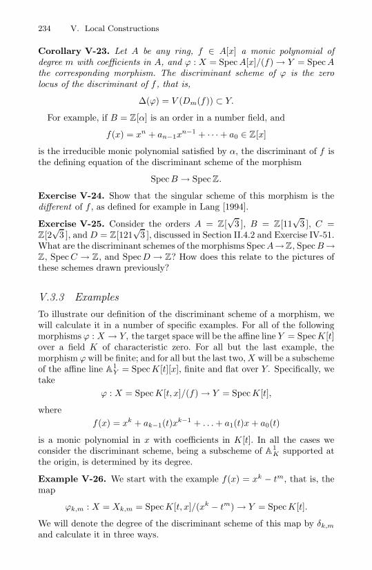
234 V. Local Constructions
Corollary V-23. Let A be any ring, f ∈ A[x] a monic polynomial ofdegree m with coefficients in A, and ϕ : X = Spec A[x]/(f) → Y = Spec Athe corresponding morphism. The discriminant scheme of ϕ is the zerolocus of the discriminant of f , that is,
∆(ϕ) = V (Dm(f)) ⊂ Y.
For example, if B = Z[α] is an order in a number field, and
f(x) = xn + an−1xn−1 + · · · + a0 ∈ Z[x]
is the irreducible monic polynomial satisfied by α, the discriminant of f isthe defining equation of the discriminant scheme of the morphism
Spec B → Spec Z.
Exercise V-24. Show that the singular scheme of this morphism is thedifferent of f , as defined for example in Lang [1994].
Exercise V-25. Consider the orders A = Z[√
3 ], B = Z[11√
3 ], C =Z[2
√3 ], and D = Z[121
√3 ], discussed in Section II.4.2 and Exercise IV-51.
What are the discriminant schemes of the morphisms Spec A→Z, Spec B →Z, Spec C → Z, and Spec D → Z? How does this relate to the pictures ofthese schemes drawn previously?
V.3.3 Examples
To illustrate our definition of the discriminant scheme of a morphism, wewill calculate it in a number of specific examples. For all of the followingmorphisms ϕ : X → Y, the target space will be the affine line Y = Spec K[t]over a field K of characteristic zero. For all but the last example, themorphism ϕ will be finite; and for all but the last two, X will be a subschemeof the affine line A1
Y = Spec K[t][x], finite and flat over Y. Specifically, wetake
ϕ : X = Spec K[t, x]/(f) → Y = Spec K[t],
wheref(x) = xk + ak−1(t)xk−1 + . . . + a1(t)x + a0(t)
is a monic polynomial in x with coefficients in K[t]. In all the cases weconsider the discriminant scheme, being a subscheme of A1
K supported atthe origin, is determined by its degree.
Example V-26. We start with the example f(x) = xk − tm, that is, themap
ϕk,m : X = Xk,m = Spec K[t, x]/(xk − tm) → Y = Spec K[t].
We will denote the degree of the discriminant scheme of this map by δk,m
and calculate it in three ways.

V.3 Singular Schemes and Discriminants 235
Note before we start that if
µα : Y = Spec K[t] −→ Y = Spec K[t]
is the map given by t → tα, we have a fiber product diagram
Xk,αm Xk,m
Y
ϕk,αm
µα
Y
ϕk,m
so that, by the invariance of the discriminant scheme under pullback,
δk,αm = α · δk,m
for any α and m.
For our first calculation of δk,m, we use the definition of the discriminantof the polynomial f(x) as the resultant of f and f ′ and apply Sylvester’sdeterminant. Thus, for example, in case k = 2 the discriminant is
δ2,m =
∣∣∣∣∣∣1 0 tm
2 0 00 2 0
∣∣∣∣∣∣ = 4tm,
so that (the characteristic of K being 0) δ2,m = m. More generally, forarbitrary k we have ak−1 = · · · = a1 = 0 and a0 = −tm. Therefore
δk,m =
∣∣∣∣∣∣∣∣∣∣∣∣∣∣∣∣∣∣∣∣∣∣∣
1 0 . . . 0 0 0 −tm 0 . . . 0 00 1 . . . 0 0 0 0 −tm . . . 0 0...
.... . .
......
......
.... . .
......
0 0 . . . 1 0 0 0 0 . . . −tm 00 0 . . . 0 1 0 0 0 . . . 0 −tm
k 0 . . . 0 0 0 0 0 . . . 0 00 k . . . 0 0 0 0 0 . . . 0 0...
.... . .
......
......
.... . .
......
0 0 . . . k 0 0 0 0 . . . 0 00 0 . . . 0 k 0 0 0 . . . 0 00 0 . . . 0 0 k 0 0 . . . 0 0
∣∣∣∣∣∣∣∣∣∣∣∣∣∣∣∣∣∣∣∣∣∣∣= (−1)k−1kk · tm(k−1),
and hence
δk,m = m(k − 1).
A second way to calculate δk,m is to use the expression of the discriminantas the product of the pairwise differences of the roots of a polynomial. Tostart, suppose that k divides m; say m = kl, and suppose also that K

236 V. Local Constructions
contains a primitive l-th root of unity ζ. Then we can factor
f(x) = xk − tkl =k−1∏i=0
(x − ζitl).
The discriminant of f is then the product
∆(f) =∏
0≤i<j≤k−1
(ζjtl − ζitl)2 =∏
0≤i<j≤k−1
(ζj − ζi)t2l,
which vanishes to order δk,m = k(k − 1)l = m(k − 1) at the origin. Thusδk,m = m(k − 1) whenever k|m; and by the formula δk,αm = α · δk,m
established above it follows that δk,m = m(k − 1) for all k and m.
Exercise V-27. The last argument uses the presence in our field K of allthe l-th roots of unity. Use a base change argument (bearing in mind thedefinition of degree!) to extend the result to any field K of characteristicnot dividing l.
Finally, we can describe the discriminant scheme of ϕ = ϕk,m directlyfrom the definition. To begin with, the sheaf of relative differentials of themap ϕ is
ΩX/Y = OXdx/(kxk−1dx),
where OXdx denotes the free OX -module with generator dx. The reso-lution of ΩX/Y is thus
0 −→ OXν−→ OX −→ ΩX/Y −→ 0
where the map ν is multiplication by xk−1. The zeroth Fitting ideal ofΩX/Y is accordingly generated by the 1× 1 minor of the matrix (xk−1), sothat the singular locus of the map ϕk,m is
sing ϕ = V (Fitt0 ΩX/Y ) = V (xk−1) ⊂ X
and Osing ϕ∼= ΩX/Y as sheaves of OX -modules.
To resolve the pushforward of the structure sheaf of sing ϕ, we can thuspush forward the exact sequence above. The pushforward ϕ∗OX is thelocally free OY -module generated by the elements α0 = 1, α1 = x, . . . ,αk−1 = xk−1. Multiplication by xk−1 takes the first generator α0 = 1 tothe last one αk−1 = xk−1, the second generator α1 = x to xk = tmα0, thethird generator α2 = x2 to xk+1 = tmα1, and so on. The resolution of thepushforward ϕ∗Osing ϕ is thus
0 −→ O⊕kY
ϕ∗ν−→ O⊕kY −→ ϕ∗Osing ϕ −→ 0

V.3 Singular Schemes and Discriminants 237
where the map ϕ∗ν is given by the matrix
ϕ∗ν =
⎛⎜⎜⎜⎜⎜⎜⎝
0 tm 0 . . . 0 00 0 tm . . . 0 00 0 0 . . . 0 0...
......
. . ....
...0 0 0 . . . 0 tm
1 0 0 . . . 0 0
⎞⎟⎟⎟⎟⎟⎟⎠
.
The discriminant scheme of ϕ = ϕk,m is the zero locus of the determinant(−1)k−1tm(k−1) of this matrix, and so we see once again that δk,m = m×(k − 1).
Note that in this setting the discriminant scheme measures not only thenumber of sheets in a branched cover that come together (that is, thenonreducedness of the special fiber, as measured by the “k − 1” factorin the expression δk,m = m(k − 1)), but also how fast they are comingtogether (the “m” factor). Thus, while in all the examples of the formX = Spec K[t, x]/(x2 − tm) → Y = Spec K[t] the fiber over the origin in Yis the same double point, the discriminant has different degrees dependingon the speed with which the two points x = ±√
tm approach each other ast approaches 0.
Here is an arithmetic analogue of this:
Exercise V-28. Reinterpret the results of Exercise V-25 in light of thecalculation in Example V-26 of the discriminant of a general projection ofa node, cusp and tacnode.
We will also see applications of Example V-26 in the discussion of dualcurves (Section V.4.2).
Although the examples we have seen so far may seem special, we can useany of the three approaches to describe the discriminant of any finite flatmorphism ϕ : X → Y where Y is nonsingular and one-dimensional and Xis locally embeddable in A1
Y , that is, for any point p ∈ X the local ring OX,p
is of the form OY,ϕ(p)[x]/(f). For example, following the second approachwe may make a base change Y ′ → Y so that the polynomial f factorscompletely into linear factors over OY (that is, the pullback X ′ = X ×Y Y ′
is a union of k irreducible components Xi, each mapping isomorphicallyto Y ). The discriminant of the pullback morphism ϕ′ : X ′ → Y ′ will thenbe given by the product of the pairwise differences of the factors of f , sothat its degree will be the sum of the degrees of the pairwise intersectionsXi ∩ Xj ; and the degree of the discriminant of ϕ at each point y ∈ Y willbe simply the sum of the degrees of the discriminant scheme of ϕ′ at thepoints y′ of Y ′ lying over y, each divided by the order of ramification ofY ′ → Y at that point.
Our next example, accordingly, will be the simplest example of a mor-phism X → Y such that X is not locally embeddable in A1
Y .

238 V. Local Constructions
Example V-29. Take Y = A1K = Spec K[t] as before, and take X the
union of three copies of A1K meeting at one point with three-dimensional
Zariski tangent space; the map ϕ will map each component of X isomor-phically to Y. We may realize X as the union of the three coordinate axesin A3
K = Spec K[x, y, z], and take ϕ : X → Y the restriction to X of theprojection map A3
K → A1K given by t → x + y + z: that is, we set
X = Spec K[t][x, y, z]/(xy, xz, yz, t−x−y−z) −→ Y = Spec K[t].
We can simplify the expression for X at the expense of some symmetry,writing
X = Spec K[t][x, y]/(xy, x(t−x−y), y(t−x−y)).
The sheaf ΩX/Y is then given as
ΩX/Y = OXdx, dy/(ydx+xdy, (t−2x)dx−xdy, −ydx+(t−2y)dy)
Since there are two generators and three relations, the resolution of ΩX/Y
takes the formO⊕3
Xν−→ O⊕2
X −→ ΩX/Y −→ 0,
where the map ν is given by the matrix
ν =(
y t − 2x −yx −x t − 2y
).
In terms of the original description X = Spec K[x, y, z]/(xy, xz, yz) of X,the 2 × 2 minors of this matrix are
−xy − x(t − 2x) = x2,
y(t − 2y) + xy = −y2, and
(t − 2x)(t − 2y) − xy = −x2 − y2 + z2,
so that the zeroth Fitting ideal Fitt0 ΩX/Y is simply the square (x2, y2, z2)of the maximal ideal of the origin in X. The singular locus sing ϕ of the mapϕ is thus the first-order neighborhood of the origin in A3
K ; in particular,it has degree 4. For any sheaf F on Y supported at the origin in A1
K ,the zeroth Fitting ideal will be simply tm, where m is the vector spacedimension of Γ(F ). The degree of the discriminant is thus equal to thedegree 4 of the singular locus.
It is also easy to describe the direct image ϕ∗Osing(ϕ) directly: since thefiber of the projection sing ϕ → Y over the origin has degree 3, we musthave
ϕ∗(Osing ϕ) = OY /(t2) ⊕ (OY /(t))⊕2,
and we can calculate the zeroth Fitting ideal Fitt0(ϕ∗Osing ϕ) accordingly.
If X had consisted of three coplanar lines meeting at a point— say, ifwe took ϕ : X = Spec K[t, x]/(x3 − t3) → Y = Spec K[t]— then by thecalculation made previously we would have deg(∆(ϕ)) = 6, while in the

V.3 Singular Schemes and Discriminants 239
spatial case we have deg(∆(ϕ)) = 4. This difference is what underlies theexample in Section II.3.4 whose general fiber is isomorphic to the three co-ordinate lines in A3
K and whose special fiber is supported on three coplanarlines: the jump in the discriminant, in a sense, forces the appearance of theembedded point in the flat limit. We saw the same phenomenon emergewhen we considered Hilbert polynomials in Sections III.3.1 and III.3.2.
Our last examples will be in the form of exercises. In them we considerthe simplest cases of a morphism ϕ : X → Y of relative dimension one,such that the singular locus sing ϕ is finite over Y.
Exercise V-30. Let K be a field of characteristic 0, let Y = Spec K[t] =A1
K , and let ϕ : X → Y be the family of curves
ϕ : X = Spec K[t][x, y]/(xy − tm) ⊂ A2Y −→ Y.
Show that the discriminant scheme ∆(ϕ) = V (tm) ⊂ Y.
In the preceding exercise, the singular curves of the families consideredhave the simplest possible curve singularity, called a node. To generalize it,we need first of all to make a definition:
Definition V-31. Let C → Spec K be a curve over an algebraically closedfield K and p ∈ C a closed point of C. We will say that p is a node, cusp ortacnode of C if the formal completion O of the local ring OC,p with respectto its maximal ideal is isomorphic to K[[x, y]]/(y2 − x2), K[[x, y]]/(y2 − x3)or K[[x, y]]/(y2 − x4) respectively.
These singularities may also be characterized geometrically: a node, forexample, is a point of C at which two smooth branches cross transversely;a tacnode is one where two smooth branches are simply tangent, that is,intersecting in a scheme of degree 2. In the case of a plane curve C ⊂ P2
K ,we will say that a node or tacnode p of C is ordinary if neither branch indi-vidually has intersection multiplicity 3 or more with its projective tangentline. (The reader may verify that if p ∈ C is a cusp, this will always be thecase.)
Exercise V-32. Let K and Y be as in Exercise V-30, and find the dis-criminant scheme ∆(ϕ) ⊂ Y for the following families ϕ : X → Y of curves:
(a) (a family acquiring a cusp)
ϕ : X = Spec K[t][x, y]/(y2 − x3 − tm) ⊂ A2Y −→ Y.
(b) (a family acquiring a tacnode)
ϕ : X = Spec K[t][x, y]/(y2 − x4 − tm) ⊂ A2Y −→ Y.
(c) (a family acquiring an ordinary k-fold point)
ϕ : X = Spec K[t][x, y]/(xk + yk − tm) ⊂ A2Y −→ Y.

240 V. Local Constructions
V.4 Dual Curves
V.4.1 Definitions
We consider now another object associated to a plane curve C ⊂ P2S : its
dual curve C∗, a subscheme of the dual projective plane (P2S)∗ as defined
in Section III.2.3. In classical algebraic geometry, the definition is simpleenough: for K an algebraically closed field and C ⊂ P2
K nonsingular ofdegree d ≥ 2, the dual curve is defined to be the set of projective tangentlines TpC to C, regarded as points of the dual projective plane (P2
K)∗. Moregenerally, for a curve C without multiple components and containing nolines the dual curve is defined to be the closure of the locus of tangent linesTpC to C at nonsingular points p of C. (In the following, we will refer tothis locus as the “classical dual”.)
As in the case of flexes (Section IV.1), what we will do here is to proposea natural set of defining equations for C∗, which will yield a definition ofthe dual C∗ ⊂ (P2
S)∗ of a plane curve C ⊂ P2S over an arbitrary scheme
S. Also as in the case of flexes, C∗ will be a closed subscheme of (P2S)∗,
flat over S over the open subset of S where it does not contain the fiber of(P2
S)∗, and invariant under base change. Our definition will agree with theclassical definition for nonsingular plane curves over fields of characteristiczero, but not for singular ones: if p is an isolated singular point of a planecurve C ⊂ P2
K , the line in (P2K)∗ dual to p will be a component of C∗ in our
definition, though it is not part of the classical dual. Again, this is necessaryif we want the duals of a family of plane curves to form a closed family; ifwe want to recover information about the classical dual, we simply discardthe extra components. (The need for characteristic zero will be explainedbelow.)
To make our definition, we have first to introduce one auxiliary object.Recall from Section III.2.8 that in the product P2
S ×S (P2S)∗ we have the
universal line Σ, whose fiber over each point l ∈ (P2S)∗ is the corresponding
line l ⊂ P2S : in terms of homogeneous coordinates X, Y, Z on P2
S and A,B, Con (P2
S)∗,Σ = V (AX + BY + CZ) ⊂ P2
S ×S (P2S)∗.
Now let C ⊂ P2S be any plane curve, and assume for the moment that C
contains no lines (that is, there is no point s ∈ S and line l ⊂ P2κ(s) in the
fiber of P2S over s contained in C; this is stronger than supposing that the
equation of C does not have a linear factor). We define the universal linesection ΓC of C to be the intersection
ΓC = π−11 (C) ∩ Σ ⊂ P2
S ×S′ (P2S)∗.
By our hypothesis that C contains no lines, the map π2 : ΓC → (P2S)∗ will
be finite (and hence flat) of degree d; and we define the dual curve C∗ ⊂(P2
S)∗ of C to be the discriminant scheme of this map, as in Definition V-21.

V.4 Dual Curves 241
Finally, if C does contain lines, we simply define C∗ to be the closure in(P2
S)∗ of the discriminant scheme of the restriction of π2 to the open subsetof (P2
S)∗ where it is finite.
A few introductory remarks are in order. To begin with, C∗ is by defi-nition a closed subscheme of (P2
S)∗, and its formation commutes with basechange: if S′ → S is any morphism and C ′ = S′ ×S C ⊂ P2
S′ , then we willhave also
ΓC′ = S′ ×S ΓC ⊂ P2S′ ×S (P2
S′)∗,
and hence C ′∗ = S′ ×S C∗. In particular, for any point s ∈ S, the fiber C∗s
of C∗ over s will be the dual of the fiber Cs ⊂ P2κ(s) of C over s.
The support of C∗ is easy to describe: by the definition of the discrimi-nant scheme of a finite morphism, it is the set of lines l ∈ (P2
S)∗ such thatthe intersection of the corresponding line l ⊂ P2
S with C is singular overκ(l). (This means either l ∩ C is nonreduced, or — in case κ(l) has charac-teristic p > 0 and is not algebraically closed— has a point whose residuefield in an inseparable extension of κ(l).) In particular, as we indicated, ifp ∈ C ⊂ P2
K is any singular point, the line in (P2K)∗ dual to p— that is,
the locus of lines in P2K passing through p — will be contained in C∗.
Finally, we remark that the “dual curve” need not be a curve! If C ⊂ P2S
is nonreduced —that is, it has a multiple component— then the dual C∗
will be all of (P2S)∗. Even if C ⊂ P2
S is nonsingular and reduced it may havenonreduced fibers Cs over some points of S. For example, the fiber of thecurve C = V (X2 + Y 2 + Z2) ⊂ P2
Z over (2) ∈ Spec Z is a double line. Insuch cases the dual C∗ will contain the corresponding fibers of (P2
S)∗, andso will not be a “plane curve” as we have defined it.
Exercise V-33. Verify that the dual C∗ of the plane curve
C = V (X2 + Y 2 + Z2) ⊂ P2Z
mentioned above is, by our definition, the subscheme
C∗ = V (4A2 + 4B2 + 4C2) ⊂ (P2Z)∗,
so is not a plane curve in (P2Z)∗.
In the example of Exercise V-33, our definition seems at first willfullyperverse: why shouldn’t we take the dual to be the zero locus of A2+B2+C2
instead? Indeed, as long as the base S is nonsingular of dimension one (as inthe exercise) any fibers of (P2
S)∗ → S contained in C∗ will be components ofC∗; we can discard them to arrive at a scheme C∗ flat over S. But we will seebelow how to construct examples of curves C ⊂ P2
S with nonreduced fibersCs over isolated points s ∈ S where this simply cannot be avoided: the fiber(P2
κ(s))∗ of (P2
S)∗ over s will be contained in the closure of C∗ ∩ (P2S\s)
∗.If we want the definition to behave well with respect to base change, thismeans the dual of Cs has to be all of (P2
κ(s))∗.

242 V. Local Constructions
Exercise V-34. Let K be a field, and C ⊂ P2K a curve, smooth over
K. Show that the dual C∗ is reduced, unless every tangent line to C ismultiply tangent— that is, has intersection multiplicity 3 or more with C,or is tangent to C at more than one point.
In fact, if the characteristic of K is zero it cannot happen that everytangent line is multiply tangent (see for example Harris [1995, Proposition15.3]), so the dual of any nonsingular plane curve will be reduced. Butthere are examples of plane curves over fields of finite characteristic suchthat every point is a flex, and other examples where every tangent line istangent at several points. In such a case, our definition yields a nonreduceddual curve C∗.
Exercise V-35. Let K be any field of characteristic zero, and C ⊂ P2K a
curve of degree d having no multiple components. Show that the dual curveC∗ ⊂ (P2
K)∗ is a plane curve of degree exactly d(d − 1).(Hint: Use the formula given in Proposition V-22 for the discriminant to
describe the intersection of C∗ with a general line in (P2K)∗.)
V.4.2 Duals of Singular Curves
In case C ⊂ P2K has isolated singular points, as we said, our definition
diverges from the classical: any line l = p∗ ⊂ P2K passing through a singular
point of C will correspond to a point in the support of the dual curve C∗.What is the multiplicity of this component? The following exercise givesthe answer in some cases, and derives as a consequence one of the classicalPlucker formulas (see Coolidge [1931]).
Exercise V-36. Using Example V-26 on discriminants, show that if p ∈ Cis a node, cusp, tacnode or ordinary triple point, then the line in p∗ ⊂ (P2
K)∗
dual to p appears with multiplicity 2, 3, 4 or 6 respectively in C∗. Deducethe Plucker formula for the degree d′ of the classical dual of an irreducibleplane curve C ⊂ P2
K over a field of characteristic zero of degree d, havingas singularities δ nodes, κ cusps, λ tacnodes and τ ordinary triple points:
d′ = d(d − 1) − 2δ − 3κ− 4λ − 6τ.
(Note that the same count is valid if C is reducible, as long as no componentof C is a line.) Find a curve singularity p ∈ C for which p∗ appears withmultiplicity 5 in the dual curve C∗.
V.4.3 Curves with Multiple Components
As in the case of flexes (Section IV.1), a very different sort of questionemerges when we consider curves with multiple components. Here, as wehave said, the definition of the dual curve C∗ yields not a curve in (P2
K)∗,but rather the whole dual plane (P2
K)∗. But we can consider a family of

V.4 Dual Curves 243
generically nonsingular curves specializing to a multiple curve and ask: insuch a family, where do the tangent lines go?
We will illustrate this problem with the same sort of curve as we usedin Section IV.1; but we will start with a simpler example: instead of afamily of quartics specializing to a double conic we will consider a family ofconics degenerating to a double line. To set it up, let K be an algebraicallyclosed field of characteristic zero, and set S = Spec K[t]. Let L(X, Y, Z) andQ(X, Y, Z) ∈ K[X, Y, Z] be homogeneous polynomials of degrees 1 and 2respectively, and assume that their zero loci in P2
K intersect transversely,that is, that V (Q, L) ⊂ P2
K is reduced. Consider the curve C ⊂ P2S given
by
π : C = Proj(K[t])[X, Y, Z]/(L(X, Y, Z)2 + tQ(X, Y, Z))
⊂ Proj(K[t])[X, Y, Z] = P2S → S.
Let C ∗ ⊂ (P2S)∗ be the dual of the curve C ⊂ P2
S . As with the scheme offlexes of the curve C, the scheme C ∗ will have two components: one, thefiber of (P2
S)∗ over the origin (t) ∈ S; and the other the closure C ′ of theinverse image in C ∗ of the punctured line T = Spec K[t, t−1] = S\(t) ⊂ S(equivalently, the closure of the dual of the curve C∩P2
T ⊂ P2T ). The scheme
C ′ will be flat over all of S, with fiber over a point (t − µ) ∈ S other thanthe origin the dual (Cµ)∗ of the curve Cµ = V (F + µG) ⊂ P2
K ; it willtherefore have as fiber over the origin a scheme C ′
0 ⊂ P2K of dimension
1 and degree 2, which we will call the “limiting position” of the duals ofthe nearby nonsingular curves Cµ as µ approaches zero. Once more, wecan translate the naive question, “where do the tangent lines to a conic gowhen the conic degenerates into a double line?” into the precise problem:determine the support of the flat limit C ′
0. The answer is expressed in thefollowing
Proposition V-37. The fiber C ′0 of C ′ over the origin (t) ∈ S consists
of the union of the two lines dual to the two points t = L = Q = 0 ofintersection of the line L = 0 and the conic Q = 0 in the plane t = 0.
Proof. We will do this by explicit calculation. To begin with, since thecharacteristic of K is not 2, we can choose affine coordinates (x, y) on theplane so that the line V (L) is the x-axis y = 0, and the conic V (Q) (if itis nonsingular) the zero locus of y2 − x2 + 1. The equation of the curveC ⊂ P2
S is then
C = V (y2 + t(y2 − x2 + 1))
and after replacing the coordinate t on S = A1K with the coordinate u =
t/(1− t) in a neighborhood of the origin and multiplying through by 1− t,we may rewrite this as
C = V (y2 − t(x2 − 1))

244 V. Local Constructions
(note that if V (Q) were singular, we could have taken this as the equationof C originally). Now, we can express any line in P2
K not passing throughthe point [0, 1, 0] (that is, the point at infinity on the y-axis) as the zerolocus of an equation
y − ax − b;
a and b are then affine coordinates on the corresponding subset A2K ⊂
(P2K)∗. The equations of the universal line section ΓC of C in the open
subset A2K × A2
K ⊂ P2K × (P2
K)∗ are then
ΓC = V (y − ax − b, y2 − t(x2 − 1)) ⊂ Spec K[a, b, x, y]
= V ((ax + b)2 − t(x2 − 1)) ⊂ Spec K[a, b, x].
Now, we may expand out the equation of ΓC as
(ax + b)2 − t(x2 − 1) = (a2 − t)x2 + 2abx + (b2 + t),
from which we see that the equation of the dual curve C ∗ is
(2ab)2 − 4(a2 − t)(b2 + t) = −4ta2 + 4tb2 + 4t2 = −4t(a2 − b2 − t).
This has, as expected, two components: the entire fiber of P2S over the
origin, and the curve C ′ given as the zero locus
C ′ = V (a2 − b2 − t) ⊂ P2S .
The intersection of this second component with the fiber of P2S over the
origin is then
C′0 = V (a2 − b2) = V (a + b) ∪ V (a − b) ⊂ P2
K .
In other words, it is the union of the two lines in (P2K)∗ dual to the points
(1, 0) and (−1, 0) of intersection of the line (y) and the conic x2 − 1 in theplane.
In fact, we can see this result from the real picture: if we draw the familyof conics y2 = t(x2 −1) specializing to the double line y = 0, we see readilythat every line through either of the points (±1, 0) is a limit of tangentlines to the curves y2 = t(x2 − 1) for small values of t; we may also writethis family of tangent lines directly. For example, the line y + x + 1 = 0through the point (−1, 0) is the limit of the line
y + x +√
1 − t = 0,
which is tangent to the curve y2 = t(x2−1). It is also clear from the picturethat any line meeting the x-axis in a point other than (±1, 0) (other than

V.4 Dual Curves 245
the x-axis itself) will be transverse to the curve y2 = t(x2 − 1) for small t.
The same sort of phenomena occur with arithmetic schemes. In fact, wehave already seen an example: the conic C = V (X2 + Y 2 + Z2) ⊂ P2
Z,which we may view as a family of conics over S = Spec Z, specializing froma nonsingular conic over the generic point of Spec Z to a double line overthe point (2) ∈ Spec Z. Here the function 2 on Spec Z plays the role ofthe variable t; we can take L(X, Y, Z) = X + Y + Z and Q(X, Y, Z) =−XY − Y Z − XZ to arrive at the curve C = V (L2 + 2Q). The onlydifference here is that fibers L(2) and Q(2) over (2) in the conic Q and theline L do not intersect in two points, but rather meet in a single point withresidue field F4. The result is expressed in the
Exercise V-38. Show that the limit of the duals of the fibers of C overSpec Z \ (2) is the line in (P2
F4)∗ corresponding to the one point of inter-
section of L(2) and Q(2) in P2F4
.
If you are curious about the duals of the quartic curves in the familyspecializing to a double conic, here is the situation:
Exercise V-39. Let K be an algebraically closed field of characteristiczero, and set S = Spec K[t]. Let Q(X, Y, Z) and G(X, Y, Z) ∈ K[X, Y, Z] bea homogeneous quadric polynomial and a homogeneous quartic polynomialrespectively such that the curves V (Q) and V (G) intersect transversely, andC ⊂ P2
S the curve given by
π : C = ProjK[t][X, Y, Z]/(Q(X, Y, Z)2 + tG(X, Y, Z))
⊂ ProjK[t][X, Y, Z] = P2S → S.

246 V. Local Constructions
Let C ∗ ⊂ (P2S)∗ be the dual of the curve C ⊂ P2
S , and C ′ the closureof the inverse image in C ∗ of the punctured line T = Spec K[t, t−1] = S \(t) ⊂ S (equivalently, the closure of the dual of the curve C ∩P2
T ⊂ P2T ).
Show that the fiber C ′0 of C ′ over the origin (t) ∈ S consists of the union
of the dual of the plane conic t = Q = 0 with multiplicity 2 with the unionof the eight lines dual to the eight points t = Q = G = 0 of intersection ofthe conic Q = 0 and the quartic G = 0 in the plane t = 0.
The general situation is this:
Exercise V-40. Let m, e and d = me be positive integers. Let F =F (X, Y, Z) and G = G(X, Y, Z) ∈ K[X, Y, Z] be respectively the equa-tions of nonsingular plane curves of degrees e and d meeting transversely,let B = Spec K[t] and consider the family of curves C = V (F m+tG) ⊂ P2
B .Show that the flat limit of the duals of the curves Ct as t approaches 0 isthe union of the dual of the curve V (F ), taken with multiplicity m, andthe duals of the points F = G = 0 of the plane curves, each taken withmultiplicity m − 1.
There is no ambiguity in specifying a plane curve Γ as its support “withmultiplicity m”: this can only mean the scheme V (F m), where Γred =V (F ).
V.5 Double Point Loci
Let ϕ : X → Y be a morphism of varieties. The double point locus of ϕ wasclassically defined to be the closure in X×X of the locus of pairs of distinctpoints p, q ∈ X with common image ϕ(p) = ϕ(q) ∈ Y. In this section wewill give a scheme-theoretic definition that, as we will see, captures moreof the geometry of the map.
For the following, we will let ϕ : X → Y be a separated morphism ofschemes. As we saw in Chapter III, the separated hypothesis means thatthe diagonal ∆X is a closed subscheme of the fiber product X ×Y X, andis satisfied for all affine and projective schemes.
Definition V-41. The double point scheme Dϕ of a separated morphismϕ : X → Y is the scheme
Dϕ = V (annI∆X ) ⊂ X ×Y X
associated to the ideal ann I∆X ⊂ OX×Y X of functions f with fI∆X = 0.
To understand this definition, recall that if ϕ : X → Y is a morphismof S-schemes (in the examples below S will be Spec K or Spec Z) andY → S is separated, then the fiber product X ×Y X is a closed subschemeof X ×S X : it is the (scheme-theoretic) inverse image
X ×Y X = (ϕ × ϕ)−1(∆Y )

V.5 Double Point Loci 247
where ∆Y ⊂ Y ×S Y is the diagonal. (Note that we have a fiber square
X ×Y X Y
X ×S X
Y ×S Y ;
∆
that is, X ×Y X is the fibered product of X ×S X and Y over Y ×S Y .)Now, away from the diagonal, the double point scheme Dϕ is simply thefiber product X ×Y X ; in particular, the closed points of its support awayfrom the diagonal are simply the pairs of distinct points p, q ∈ X suchthat ϕ(p) = ϕ(q). In this sense it generalizes the classical double pointlocus, though it may have nontrivial scheme structure even in case ϕ isa morphism of varieties. In addition, as our examples will show, it mayhave components supported on the diagonal ∆X ⊂ X ×S X — that is, itssupport may properly contain the double point locus — and may even benonempty in cases where the classical double point locus is empty.
Example V-42. Consider the maps from X = A1K = Spec K[t] to Y =
A2K = Spec K[x, y] given by polynomials of degree 3, mapping X onto plane
cubic curves with a node or a cusp. Specifically, consider for each value ofthe parameter λ the map ϕλ : X → Y given by the ring homomorphism
ϕ#λ : K[x, y] −→ K[t]
x −→ t2 − λ
y −→ t3 − λt.
The image of ϕλ is the plane curve Cλ with equation y2 = x2(x + λ).
λ = 1 λ = 12
λ = 0

248 V. Local Constructions
The fiber product X ×Y X is the spectrum Spec R of the algebra
R = K[t1] ⊗K[x,y] K[t2]
= K[t1, t2]/((t21 − λ) − (t22 − λ), (t31 − λt1) − (t32 − λt2)
)= K[t1, t2]/
((t1 − t2)(t1 + t2, t
21 − λ)
).
By our definition, then, the double point scheme Dϕ of ϕ = ϕλ is given by
Dϕ = V(ann((t1 − t2)/((t1 − t2)(t1 + t2, t
21 − λ)))
)= V ((t1 + t2, t
21 − λ)) ⊂ Spec K[t1, t2] = X ×K X.
Assuming that the characteristic of K is not 2, for λ = 0, Dϕ consists ofthe two reduced points (
√λ,−√
λ) and (−√λ,
√λ). For λ = 0, on the other
hand, Dϕ is a double point supported at the origin. (Note that Dϕ0 is theflat limit of the schemes Dϕλ
for λ = 0 as λ approaches 0.)To see the difference between the classical and modern approaches, ob-
serve that for λ = 0 the scheme X ×Y X , as pictured in the figure below,is reduced; hence the double point scheme is reduced as well and coincideswith the classical double point locus. For λ = 0, however, they differ: thescheme X ×Y X consists of the diagonal in X ×K X, plus an embeddedpoint supported at the origin. In the classical language, we see only thereduced scheme associated to X ×Y X, and so miss the embedded point;thus the double point locus of ϕ0 is empty. Scheme theory, by contrast,does see the nonreduced structure of X ×Y X and as a result the doublepoint scheme of ϕ0 is nonempty, reflecting the fact that ϕ0 fails to be animmersion at t = 0.
λ = 0 λ = 0
t1 t1
t2 t2
To make somewhat more precise the remark above that the nonempti-ness of the double point scheme of ϕ0 reflects the fact that ϕ0 is not animmersion, we have the following two exercises.
Exercise V-43. Let ϕ : X → Y be a finite map of nonsingular varietiesover an algebraically closed field K of characteristic zero, and Dϕ its doublepoint scheme. Show that
supp (Dϕ ∩ ∆X) = (p, p) : Ker(dϕp) = 0 ⊂ X ×K X.

V.5 Double Point Loci 249
Exercise V-44. Let ϕ : X → Y again be a finite map of irreducible vari-eties and Dϕ its double point scheme. Using Harris [1995, Theorem 14.9],we see that in fact ϕ is an embedding if and only if Dϕ = ∅, that is, if andonly if
(ϕ × ϕ)−1(∆Y ) = ∆X
as schemes (which is to say, X → X ×Y X is an isomorphism).
Here is an exercise showing that the same geometric ideas apply as wellin the context of arithmetic schemes: the schemes in question are spectraof rings of integers in number fields (they were first introduced in Sec-tion II.4.2), but as we will see they behave very much like the curves de-scribed in the example above.
Exercise V-45. Consider the maps
ϕ : Spec Z[11√
3] −→ A1Z
andµ : Spec Z[2
√3] −→ A1
Z
associated to the maps Z[t] → Z[11√
3] and Z[t] → Z[2√
3]. Describe thedouble point scheme of each map, and in particular reconfirm the assertionof Exercise II-36 that the singularity of the former is a node, while that ofthe latter is a cusp.
Finally, we point out also that nonreduced structures on the double pointlocus arise naturally even away from the diagonal in X×X, for example formaps ϕ that are immersions. For example, consider the case where Y is acurve and ϕ : X → Y its normalization. Suppose that two points P, Q ∈ Xmap to the same point R of the image curve Y = ϕ(X).
Exercise V-46. Show that if R is a node, the double point scheme willbe reduced at the point (P, Q) ∈ X × X. By contrast, show that if R is atacnode (that is, Y has two smooth branches at R, simply tangent to oneanother) Dϕ will be nonreduced at the point (P, Q) ∈ X × X. Can youdescribe the scheme structure?

VISchemes and Functors
At the end of the first chapter of this book we discussed a way of embeddingthe category of schemes into the larger category of contravariant functorsF from the category of schemes to the category of sets.
This embedding is useful in at least three ways:(1) The effect of some basic constructions, such as products, is much easier
to describe on functors of points than on schemes.(2) In trying to construct a certain scheme, it is often easy to construct
the functor that would be the functor of points of that scheme, ifthe scheme existed; the construction problem is then reduced to theproblem of proving that the functor is representable and the use ofYoneda’s Lemma (VI-1). The process is exactly analogous to the useof distributions in analysis: there, when trying to prove the existenceof a nice function solving a given differential equation, one first provesthe existence of a solution that is a distribution, and then is left withthe (possibly more tractable) regularity problem of proving that thedistribution is represented by integration against a function.
(3) Many aspects of the geometry of schemes can be extended to the cat-egory of functors, so that it is sometimes useful to forget about repre-senting a functor and work in that category (or some suitable subcat-egory) directly.
In this chapter we illustrate these points, first with some basic construc-tions, and then with some examples coming from the desire to parametrizefamilies of schemes. We shall see in Section VI.2.4 that some of these leadto functors that are not actually schemes, though they are rather close.

252 VI. Schemes and Functors
VI.1 The Functor of Points
We start where we left off at the end of Chapter I. Recall that the functorof points of a scheme X is the functor
hX : (schemes) → (sets)
where (schemes) and (sets) represent the category of schemes with thearrows reversed and the category of sets; hX takes each scheme Y to theset
hX(Y ) = Mor(Y, X)
and each morphism f : Y → Z to the map of sets
hX(Z) → hX(Y )
defined by sending an element g ∈ hX(Z) = Mor(Z, X) to the compositiong f ∈ Mor(Y, X). We say that a functor F : (schemes) → (sets) isrepresentable if it is of the form hX for some scheme X. By Yoneda’s Lemmabelow, X is unique if it exists; in this case we say that X represents F.The set hX(Y ) is called the set of Y -valued points of X (if Y = Spec T isaffine, we will often write hX(T ) instead of hX(Spec T ) and call it the setof T -valued points of X).
Recall also that this construction defines a functor
h : (schemes) → Fun((schemes), (sets))
(where morphisms in the category of functors are natural transformations),sending
X → hX
and associating to a morphism f : X → X ′ the natural transformationhX → hX′ that for any scheme Y sends g ∈ hX(Y ) = Mor(Y, X) to thecomposition f g ∈ hX′(Y ) = Mor(Y, X ′).
In order for this notion to be of any use at all, a crucial first fact is thatthe functor of points hX really does determine the scheme X. This followsfrom a basic categorical fact.
Lemma VI-1 (Yoneda’s Lemma). Let C be a category and let X, X ′ beobjects of C.
(a) If F is any contravariant functor from C to the category of sets, thenatural transformations from Mor(−, X) to F are in natural correspon-dence with the elements of F (X).
(b) If the functors Mor(−, X) and Mor(−, X ′) from C to the category ofsets are isomorphic, then X X ′. More generally, the maps of functorsfrom Mor(−, X) to Mor(−, X ′) are the same as maps from X to X ′;that is, the functor
h : C → Fun(C , (sets))

VI.1 The Functor of Points 253
sending X to hX is an equivalence of C with a full subcategory of thecategory of functors.
Proof. For part (a), the correspondence sends α : Mor(−, X) → F to theelement α(1X), where 1X : X → X is the identity map. The inverse takesp ∈ F (X) to the map α sending an element f ∈ Mor(Y, X) to F (f)(p) ∈F (Y ). As for part (b), we can apply the statement of part (a) to the functorF = Mor(−, Y ).
The following improvement of Lemma VI-1 shows that it is enough tolook at the functor of points restricted to the category of affine schemes, or,equivalently, to the category (rings), the category of commutative ringswith the arrows reversed; and the same thing works in the relative setting.
Proposition VI-2. If R is a commutative ring, a scheme over R is de-termined by the restriction of its functor of points to affine schemes overR; in fact
h : (R-schemes) → Fun((R-algebras), (sets))
is an equivalence of the category of R-schemes with a full subcategory ofthe category of functors.
Of course, a contravariant functor on the category of affine schemes isthe same as a covariant functor on the category of rings; so given thisresult, we will generally think of our contravariant representable functorshX : (schemes) → (sets) as covariant functors on R-algebras. (If we needto make a distinction, we will denote by h∗
X : (rings) → (sets) the functordefined by h∗
X(A) = hX(Spec A) for any R-algebra A.)
Proof. This is really just the statement that schemes are built up out ofaffine schemes. Let S = Spec R. Write hX for the functor MorS(−, X) re-stricted to the category of affine schemes over S. It is enough to show thatany natural transformation ϕ : hX → hX′ comes from a unique morphismf over S from X to X ′. To construct f from ϕ, let Ua be an affinecover of X, and apply ϕ to the inclusion maps Ua ⊂ X to get morphismsUa → X ′. These morphisms satisfy the compatibility conditions necessaryto define the desired morphism f . Uniqueness comes down to the obser-vation that two morphisms from X to X ′ that differ are already differentwhen restricted to one of the Ua.
Exercise VI-3. Suppose that X is (like virtually all schemes of interestto us) locally Noetherian — that is, covered by spectra of Noetherian rings.Prove that X is determined by the restriction of hX to the category ofNoetherian rings.

254 VI. Schemes and Functors
VI.1.1 Open and Closed Subfunctors
One reason that thinking of schemes as functors is useful is that it is pos-sible to extend some of the basic notions from the geometry of schemes tofunctors. We will consider some examples.
We first show how to define an open subfunctor of a functor
F ∈ Fun((rings), (sets)).
We say that a map α : G → F of functors from a category C to the categoryof sets is injective if for every object X the induced map of sets G(X) →F (X) is injective (this corresponds to the standard categorical notion, butwe will not need this fact). In this case we will say that α : G → F is asubfunctor of F. For example, if U ⊂ X is a subscheme, the functor hU
will be a subfunctor of hX .We want to define an open subfunctor of a functor F to be a subfunctor
that, when restricted to a representable subfunctor hX ⊂ F , is of the formhU ⊂ hX for an open subscheme U ⊂ X . To carry this out, we need tointroduce the notion of a fibered product of functors.
Definition VI-4. If A, B, and C are functors from some category C tothe category of sets and if f : A → C and g : B → C are morphisms offunctors, the fibered product A×C B is the functor from C to (sets) definedby setting, for any object Z of C,
(A ×C B)(Z) = (a, b) ∈ A(Z) × B(Z) | f(a) = f(b) in C(Z),and defined on morphisms of C in the obvious way.
Definition VI-5. A subfunctor α : G → F in Fun((rings), (sets)) is anopen subfunctor if, for each map ψ : hSpecR → F from the functor repre-sented by an affine scheme Spec R (that is, each ψ ∈ F (R)), the fiberedproduct
Gψ hSpecR
G α F
ψ
of functors yields a map Gψ → hSpec R isomorphic to the injection from thefunctor represented by some open subcheme of Spec R.
Exercise VI-6. Let X = Spec R be an affine scheme. Show that the opensubfunctors of hX are exactly the functors of the form
F (T ) = ϕ ∈ hX(T ) | ϕ∗(I)T = T ,for some ideal I ⊂ R.
Exercise VI-7. Let X be a scheme over the field K. Define a functorF : (schemes/K) → (sets) as follows: for each K-scheme Y, let F (Y ) be

VI.1 The Functor of Points 255
the set of closed subschemes Z ⊂ X ×K Y flat over Y and such that all thefibers of Z over closed points of Y are subschemes of degree 2 of X. Let Gbe the subfunctor of F obtained by adding the requirement that the fibersof Z over closed points of Y are reduced. Show that G ⊂ F is open.
To define closed functors, we proceed similarly. A subfunctor α : G → Fin Fun((rings), (sets)) is closed if for each map ψ : hSpec R → F the fiberedproduct of ψ and α is a subfunctor of hSpec R isomorphic to the functorrepresented by a closed subcheme of Spec R.
Exercise VI-8. Let X = Spec R be an affine scheme. Show that the openand closed subfunctors of hSpecR are precisely those represented by openand closed subschemes of Spec R. (The same is true, and only a little harder,for arbitrary schemes.)
As usual, a little caution is necessary when using these notions. Forexample:
Exercise VI-9. Suppose that F is a functor from a category C to thecategory of sets, and let G be a subfunctor of F . Show by example that theassociation C → F (C) \G(C) may not define a functor. Suppose now thatC is the category of rings and F is represented by a scheme X while G isrepresented by a closed subscheme Y of X , and H is the functor reprsentedby the open subscheme X \ Y . Can you describe H in terms of G and F?
Exercise VI-10. Let X be a scheme over the field K. Define the functorF : (scheme/K) → (sets) as in Exercise VI-7, and define a subfunctor Hof F by letting H(Y ), for each K-scheme Y, be the set of closed subschemesZ ⊂ X × Y flat over Y and such that all the fibers of Z over closed pointsof Y are subschemes of degree 2 of X supported at a single point of X.Show that H is not in general a closed subfunctor of F.
We will also use the notion of an open covering of a functor. This is acollection of open subfunctors that yields an open covering of a schemewhenever we pull back to a representable functor. More precisely: let F :(schemes) → (sets) be a functor. Consider a collection Gi → F of opensubfunctors of F . For each map hx → F from a representable functorhX to F , there are open subschemes Ui ⊂ X such that the fiber producthX ×F Gi of hX and Gi is hUi . We say that the collection Gi → F isan open covering if, for any such map hX → F , the corresponding opensubschemes Ui ⊂ X cover X.
One warning: if Gi → F is an open covering of F , it is not necessarilythe case that F (T ) =
⋃Gi(T ) for all schemes T . (For example, consider
F = hSpec Z , G1 = hSpecZ[1/p], G2 = hSpecZ[1/q],
where p and q are distinct primes. Then Gi → F is an open covering, butF (Spec Z) consists of one point (the identity map), whereas Gi(Spec Z) =∅ for i = 1, 2.) However, it is the case that an open covering Gi → F

256 VI. Schemes and Functors
yields a covering F (T ) =⋃
Gi(T ) for sufficiently local flat schemes T . Forexample:
Exercise VI-11. Let Gi → F be a collection of open subfunctors of afunctor F : (schemes) → (sets). Show that this is an open covering if andonly if F (Spec K) =
⋃Gi(Spec K) for all fields K.
VI.1.2 K-Rational Points
If X is a scheme over a field K, the K-valued points of X over K are mapsSpec K → X whose composition with the natural map X → Spec K is theidentity. We claim that such maps correspond exactly to closed points p ofX that are rational over K (or K-rational) in the sense that the residueclass field κ(p) is K (via the inclusion map of K into the local ring of Xat p). Indeed, since Spec K has no nontrivial open coverings, a map fromSpec K into X is a map into some affine open subscheme Spec T of X, andsuch a morphism is determined by a K-algebra map T → K — that is, by amaximal ideal of T with residue class field K. Conversely, we may reversethe construction and see that any K-rational closed point p gives rise to aunique morphism Spec K → X of K-schemes.
We reiterate the warning about working in the category of S-schemesrather than the category of all schemes, where applicable. For example,when working with complex varieties, one would expect hSpec C(Spec C) tobe a single point (the identity map)— and this is true in the category ofC-schemes. But in the category of schemes, this set is very large!
Exercise VI-12. Let X = Spec C, considered as an abstract scheme, thatis, a scheme over Z. Describe the set hX(Spec C) of all C-valued points ofSpec C.
VI.1.3 Tangent Spaces to a Functor
Sometimes it is much easier to compute geometric information about ascheme if one knows its functor of points than if one knows its equations!A typical example occurs with the Zariski tangent space. (We will see thisapplied in Section VI.2.3).
We will work with schemes over a fixed field K, and all morphisms willbe morphisms over K.
Recall that if X is a scheme, then for any K-rational point p ∈ X theZariski tangent space to X at p is HomK(m/m2, K), where m = mX,p isthe maximal ideal in the local ring of X at p and K = κ(p) = OX,p/mX,p
is the residue field of X at p. Now let X be a scheme over K. Let X be theaffine scheme Spec K[ε]/(ε)2. We claim that a K[ε]/(ε)2-valued point of Xis the same as a K-rational closed point p of X together with an elementof the Zariski tangent space to X at p.

VI.1 The Functor of Points 257
To check this assertion, note first that because of the inclusion mapι : Spec K → Spec K[ε]/(ε2) induced by the algebra map K[ε]/(ε2) → K,a morphism Spec K[ε]/(ε2) → X determines a morphism Spec K → Xand thus a closed, K-rational point p of X. An extension of such a mor-phism Spec K → X consists of a lifting of the K-algebra homomorphismOX,p → κ(p) = K to a (local) homomorphism OX,p → K[ε]/(ε2). Such ahomomorphism induces a map from the maximal ideal mX,p to the maxi-mal ideal (ε) of K[ε]/(ε2), and since (ε2) = 0, this map factors through amap t : mX,p/m2
X,p → (ε) ∼= K. The map t is an element of (mX,p/m2X,p)
∗,the Zariski tangent space to X at p.
Conversely, given a K-rational point p ∈ X and t : mX,p/m2X,p → (ε) ∼=
K we may construct a map OX,p → K[ε]/(ε2) from the map π : OX,p →κ(p) = K corresponding to p, as follows: π and the K-algebra structuremap K → OX,p define a K-vector space splitting of OX,p/m2
X,p into K ⊕mX,p/m2
X,p; and we use the identity map on K and the map t on mX,p/m2X,p
to define a map
OX,p/m2X,p → K[ε]/(ε2),
which by composition with the projection gives a map OX,p → K[ε]/(ε2).This map determines the desired morphism of schemes Spec K[ε]/(ε2)→X.
In Section VI.2.1 we will see how this characterization of tangent vectorsto a scheme may be used to give an intrinsic description of tangent vectorsto projective space, completing the discussion in Section III.2.4.
If now F is a functor from the category of K-algebras to (sets) andp ∈ F (K), we may define the tangent space TpF to F at p to be the fiberover p in F (K[ε]/(ε2)) → F (K). One objection that may be raised to thisdefinition is that it gives us the tangent space as a set, rather than as avector space over K. One can at least define multiplication by elements ofK: if a ∈ K, then the map ε → aε induces an endomorphism of the algebraK[ε]/ε2, making the diagram
ε aε
K[ε]/(ε2) K[ε]/(ε2)
K
commute; and this induces a map TpF → TpF, which is the desired mul-tiplication by a. To make TpF a vector space, we now need to define anaddition map TpF × TpF → TpF. In general, there seems to be no way todo this; but for those functors F that, like representable functors, preservefibered products, we can.
To do this, consider the scheme Spec K[ε′, ε′′]/(ε′, ε′′)2 — that is, theclosed subscheme of the plane given by the square of the maximal ideal

258 VI. Schemes and Functors
of a point. The commutative diagram
K[ε′]/(ε′)2
K[ε′, ε′′]/(ε′, ε′′)2
K
K[ε′′]/(ε′′)2
given by the projections expresses K[ε′, ε′′]/(ε′, ε′′)2 as the fibered productover K of K[ε′]/(ε′)2 and K[ε′′]/(ε′′)2. On the other hand, there is a thirdmap, σ : K[ε′, ε′′]/(ε′, ε′′)2 → K[ε]/(ε2), that takes both ε′ and ε′′ to ε.Thus if the functor F preserves fibered products in the category of algebras,or even just the fibered product given above, we can form the diagram
F (K[ε′]/(ε′)2)×F (K)F (K[ε′′]/(ε′′)2) == F (K[ε′, ε′′]/(ε′, ε′′)2)F (σ) F (K[ε]/(ε)2)
F (K)
and taking fibers over p ∈ F (K), we get the desired addition map.
Exercise VI-13. Verify that these maps make TpF into a K-vector space,and that this is the old vector space structure in the case where F is arepresentable functor.
VI.1.4 Group Schemes
It is extremely easy to specify extra structure on a scheme by specifying iton the functor. For example, we may define a group scheme as a scheme Gand a factorization of the functor hG(rings) → (sets) through the forget-ful functor (groups)→ (sets)— that is, a group scheme is a scheme and anatural way of regarding Mor(X, G) as a group for each X.
By Yoneda’s Lemma (VI-1), this is the same thing as giving maps
G × G → G, G → G and Spec K → G
representing the multiplication, inverse, and identity element, respectively,and satisfying the usual laws (associativity and so on), but is often muchsimpler. For example, GLn can be defined as the affine scheme of invertibleintegral n × n matrices,
Spec Z[xij ][det(xij)−1],
but one usually thinks of it as a functor that associates to every ring T thegroup GLn(T ). The interesting point here is just that this family of groupsalready specifies the structure of a scheme and the additional structuremaps!

VI.2 Characterization of a Space by its Functor of Points 259
VI.2 Characterization of a Space by its Functor ofPoints
It is often much easier, and sometimes more illuminating, to describe thefunctor of points of an interesting scheme than to give a direct constructionof it, whether by gluing or by explicit equations in affine or projectivespace. Typical examples come from the Hilbert scheme and other moduliproblems, where one wants a natural space whose points represent somegeometric objects. However, the point of view is also useful in discussingmuch simpler objects, such as fibered products, or projective space itself.
The basic idea in any case is to first define a functor from the categoryof schemes to the category of sets, and then to prove an existence theoremasserting that there is a scheme of which it is the functor of points. Ofcourse, to carry this procedure out an essential ingredient is a local (andreadily verifiable) criterion for a functor to be representable, and we startby giving such a criterion.
VI.2.1 Characterization of Schemes among Functors
To the extent that we want to define and/or construct schemes first asfunctors, we run into a fundamental problem, that of determining when afunctor comes from a scheme. Here is one characterization.
We say that F : (rings) → (sets) is a sheaf in the Zariski topology if foreach ring R and each open covering of X = Spec R by distinguished openaffines Ui = Spec Rfi the functor F satisfies the sheaf axiom for the opencovering
⋃Ui = X. That is, for every collection of elements αi ∈ F (Rfi)
such that αi and αj map to the same element in F (Rfifj ), there is a uniqueelement α ∈ F (R) mapping to each of the αi.
This is a reasonably easy property to check in practice. It is in factenough to guarantee that F comes from a scheme if we know already thatF is covered by affine schemes in the following sense. The reader may provethe following theorem.
Theorem VI-14. A functor F : (rings) → (sets) is of the form hY forsome scheme Y if and only if
(1) F is a sheaf in the Zariski topology, and
(2) there exist rings Ri and open subfunctors
αi : hRi → F
such that, for every field K, F (K) is the union of the images of hRi(K)under the maps αi.
As an easy application, one can use the theorem to show the existence offibered products. The construction of fibered products in the category ofschemes, which was explained in Chapter I, is of fundamental importance,

260 VI. Schemes and Functors
but it is surprisingly clumsy. Using the functorial point of view, we canat least describe the fibered product of two schemes by giving its functorof points directly. If X → S and Y → S are morphisms of schemes, thefibered product X×S Y is determined by saying that it is the scheme whosefunctor of points is the fibered product of functors hX ×hS hY . Its existenceis established in the following exercise.
Exercise VI-15. (a) Show that if f : A → C and g : B → C are mor-phisms of functors all of which are sheaves in the Zariski topology, thefibered product A ×C B is a sheaf in the Zariski topology.
(b) Use the open covering of the fibered product suggested in Chapter Iand the above theorem to prove the existence of fibered products inthe category of schemes.
The next example gives a different way of looking at maps to projec-tive spaces. Theorem III-37 may be translated immediately into our newlanguage:
Theorem VI-16. If Y = PnZ, then
hY (X) =
locally free subsheaves F ⊂ On+1X
that locally are summands of rank n
=invertible sheaves P on X with an epimorphism On+1
X → Pisomorphisms ,
where isomorphism is defined as in Corollary III-42.
By way of an application, we will combine this description of maps toprojective space with the characterization in Section VI.1.3 of tangent vec-tors to a scheme X as maps of Spec K[ε]/(ε2) to X to compute the Zariskitangent spaces to Pn
K at K-valued points. By what we have just said, aK-valued point of Pn
K is a rank n summand F ⊂ Kn+1; let L be the quo-tient L = Kn+1/F. The Zariski tangent space T at this point is the set ofall summands F ′ ⊂ (K[ε]/(ε)2)n+1 that restrict to F modulo ε. We claimthat there is a natural isomorphism
T ∼= HomK(F, L).
To produce it, choose a splitting Kn+1 = F ⊕ L and a basis ei of F. Anysummand F ′ of (K[ε]/(ε)2)n+1 that reduces mod ε to F has a basis of theform ei + εsi + εti with si in F and ti in L, say. We associate to K ′ themap α : F → L sending ei to ti. Conversely, given any map α, we maydefine F ′ to be the module spanned by the elements ei + εα(ei).
Exercise VI-17. Check that these definitions are independent of all thechoices made.
Finally, Theorem VI-14 can also be used to prove the existence of theGrassmannian scheme from its functorial description.

VI.2 Characterization of a Space by its Functor of Points 261
Exercise VI-18. For 0 < k < n, let
g = g(k, n) : (rings) → (sets)
be the Grassmannian functor, that is, the functor given by
g(T ) = rank k direct summands of T n.Prove that this is the functor of points of a closed subscheme GZ(k, n) ofprojective space Pr
Z, called the Grassmannian of k-planes in n-space, asfollows.
First, let r =(nk
) − 1, and let PrZ = ProjZ[. . . XI . . .] be the projective
space with homogeneous coordinates XI corresponding to the subsets ofcardinality n− k in 1, 2, . . . , n. Define a natural transformation g → hPr
Z
of functors by sending a summand M ⊂ T n to∧k M ⊂ ∧k T n. Cover Pr
Z
by the usual open affine subschemes UI∼= Ar
Z ; show that these subschemesare represented by the subfunctors
UI(T ) =
rank r summands of T r+1 such that the I-thbasis vector of T r+1 generates the cokernel
and that the intersection (fiber product) of UI and g is the functor
(UI ∩ g)(T ) =
rank k summands M of T n such that the basisvectors ei1 , . . . , ein−k
∈T n generate the cokernel
.
Check that the intersection UI ∩g is represented by an affine scheme. Showthat g is a sheaf in the Zariski topology, and conclude that g is representedby a scheme.
Note once more that we do not have g(T ) =⋃
(UI ∩ g)(T ), except onlocal rings.
Exercise VI-19. Show that this definition of the Grassmannian coincideswith the one given in Section III.2.7.
Exercise VI-20. For a field K, give an analogous definition of the Grass-mannian GK(k, n), and show that it coincides with the product GZ(k, n)×Spec K.
We will see other examples of the use of this theorem in the next section.The functorial point of view is developed in far greater depth and detail inDemazure and Gabriel [1970], to which the interested reader is referred formore information.
One of the principal goals in Grothendieck’s work on schemes was tofind a characterization of scheme-functors by weak general properties thatcould often be checked in practice and so lead to many existence theoremsin algebraic geometry (like Brown’s theorem in the homotopy category; seeSpanier [1966, Chapter 7.7]). It seemed at first that this program wouldfail completely and that scheme-functors were really quite special; see Hi-ronaka [1962], for instance. Artin, however, discovered an extraordinary

262 VI. Schemes and Functors
approximation theorem exhibiting a category of functors F only “a little”larger than the scheme-functors that can indeed be characterized by weakgeneral properties. Geometrically speaking, the functors F are like spacesobtained by dividing affines by “etale equivalence relations” and then glu-ing. He calls them algebraic spaces (for a typical occasion where they arise,see Section VI.2.4). For details, see Artin [1971] and Knutson [1971].
VI.2.2 Parameter Spaces
The Hilbert Scheme. Probably the one area where the notion of thefunctor of points has had the most impact is in the construction and de-scription of parameter spaces. We have already mentioned in Section III.3.3,for example, that the subschemes of a projective space Pn
K over a field Khaving a given Hilbert polynomial P form a scheme, which we will call HP .It seems surprising that such a statement has an unambiguous meaning.While it is intuitively plausible that the set of such objects might form thepoints of a variety, couldn’t they form a variety in several different ways?And in what sense do they form a scheme?
The answers are obtained by making precise what properties we wantthe correspondence between the set of subschemes and the set of points ofHP to have. Specifically, note that if X ⊂ Pn
K ×B → B is any flat familyof subschemes of Pn
K with Hilbert polynomial P, we get a map from thepoints of B with residue field K to the points of HP with residue field K,sending a point b ∈ B to the point of HP corresponding to the fiber Xb
of HP over b. It is natural to ask that this map come from a regular mapB → HP . Carrying this a little further, we want HP to have the propertythat for any scheme B over K, the set of flat families of subscheme of Pn
K
with Hilbert polynomial P parametrized by B is naturally identified withthe set of maps from B to HP . Finally, since the problem of parametrizingsubschemes of Pn
K with a given Hilbert polynomial should be in some sensethe same for all K, we would like to do this over Spec Z — that is (as inthe case of the Grassmannian, which is indeed a special case of a Hilbertscheme) define for each P a single object HP over Spec Z such that for anyK the product HP × Spec K parametrizes subschemes of Pn
K with Hilbertpolynomial P.
To say this a little differently, we make the following definition:
Definition VI-21. The Hilbert functor hP — called the “functor of flatfamilies of schemes in Pn
Z with Hilbert polynomial P”— is the functor
hP : (schemes) → (sets)
that associates to any B the set of subschemes X ⊂ PnB flat over B whose
fibers over points of B have Hilbert polynomial P.
We then want to take the Hilbert scheme HP to be the scheme thatrepresents hP : in other words, the scheme whose functor of points is hP .

VI.2 Characterization of a Space by its Functor of Points 263
By Yoneda’s Lemma (VI-1), this determines the scheme HP , if one suchexists; the key theorem is thus the following.
Theorem VI-22. There exists a scheme HP whose functor of points isthe functor hP .
Note that for any scheme S we can make an analogous definition of afunctor hP,S : (S−schemes) → (sets) on the category of S-schemes, andthat if HP is the scheme representing the functor hP as above, then hP,S
is represented by the S-scheme HP × S.In fact, it turns out that HP ×Spec K is often a scheme that is genuinely
not a variety. We will describe, in Exercises VI-35 through VI-37, a famousexample of Mumford [1962] of a Hilbert scheme that is nonreduced even atpoints corresponding to nonsingular, irreducible projective varieties.
The statement of Theorem VI-22 has another interpretation that is oftenuseful: saying that the functor hP is representable is the same thing assaying that there exists a universal family — that is, a scheme H and asubscheme X ⊂ Pn
Z × H flat over H with Hilbert polynomial P — suchthat any subscheme Y ⊂ Pn
Z × B flat over B with Hilbert polynomial P isequal to the fiber product Y = X ×H B ⊂ Pn
Z ×B for a unique morphismB → H . Clearly, if a universal family X ⊂ Pn
Z × H exists, then Hrepresents the functor hP . Conversely, if a scheme H represents hP , thenthe subscheme X ⊂ Pn
Z × H associated to the identity map is universalin the above sense.
We will not give a proof of Theorem VI-22 but will indicate how it maybe approached; for more details we refer the reader to Mumford [1966] orKollar [1996].
The idea is easy to summarize: reducing to the case of a subschemeX of projective space Pn
B over a base of the form B = Spec R with Ra local ring, such a scheme X is determined by its ideal I(X) ⊂ S =R[X0, . . . , Xn], which in turn is determined for m sufficiently large (in asense depending only on P ) by its degree m piece I(X)m ⊂ Sm. SettingM =
(m+n
n
)and q = P (m), this in turn corresponds to a point in the
Grassmannian GB(q, M) parametrizing summands of codimension P (m)in the free R-module Sm
∼= RM. In this way HP,B becomes a subschemeof the Grassmannian GB(q, M) of such planes.
The key point is that we can choose a single m that has this propertyuniformly for every subscheme X with Hilbert polynomial P ; that is, thatfor every P, there is an m0 such that if m ≥ m0 and X is a subscheme ofPn
K with Hilbert polynomial P, then I(X)l≥m is generated by I(X)m, andthe codimension of I(X)m in Sm is PX(m). Examining our proof that theHilbert polynomial is a polynomial, we see that to prove this it is enough toshow that the degrees of the generators of the free modules in the minimalfree resolution of I(X) can be bounded in terms of the Hilbert polynomial

264 VI. Schemes and Functors
of X. This is done by using the idea of Castelnuovo regularity of X ; a morecomplete description would take us too far afield.
We thus have, for every flat family X ⊂ PnB over a base B = Spec R —
that is, an element of hP (Spec R)—a summand of corank q in RM —thatis, an element of the set g(q, M)(R), where g = g(q, M) is the Grassmannianfunctor as defined in Exercise VI-18. This association extends to a naturaltransformation of functors from h∗
P to g(q, M), where h∗P : (rings) → (sets)
is the functor h∗P (R) = hP (Spec R), and hence to a natural transformation
from the Hilbert functor hP to the functor respresented by the Grassman-nian G = GZ(q, M).
To finish the argument, one must show that there exists a subschemeHP ⊂ G such that a morphism ϕ : B → G comes in this way from a flatfamily X ⊂ Pn
B with Hilbert polynomial P if and only if ϕ factors throughHP . We will content ourselves here with describing the equations of HP
as a closed subscheme of G. Let Y be the universal subbundle on G. Wehave multiplication maps
multk : Y ⊗ Sk → Sk+m,
where S = Z[X0, . . . , Xn], and we can take HP to be the “determinantal”subscheme of GZ(q, M) defined by the conditions that
rank(multk) ≤ dim Sk+m − P (m + k)
for all k ≥ 0. It is immediate that the desired maps ϕ all factor through thissubscheme. Given any point p in this subscheme, one shows that (becausem has been chosen so large) the ideal generated by the corresponding linearsubspace of Sm defines a scheme with Hilbert polynomial P. This gives us a“tautological family” on HP of schemes with Hilbert polynomial P. Givenany map ϕ from a scheme B into HP , one can “pull back” this family byusing the fibered product to get a family over B, and the map ϕ will beassociated to this family. Once all this is verified, the description of HP byits functor of points ensures that HP does not depend on the choice of m.
Examples of Hilbert Schemes. We will mention, largely in the form ofexercises, some examples of Hilbert schemes. To begin with, the Grassman-nian GS(k, n) is a Hilbert scheme: it parametrizes subschemes X of degree1 and dimension k (specifically, with Hilbert polynomial P (m) =
(m+k
k
))in the projective space Pn
S . The following exercise deals with the simplestspecial case of this, but the general statement (and proof) differs only nu-merically.
Exercise VI-23. Let P (m) = m + 1 be the Hilbert polynomial of a line.Show that the Hilbert scheme of subschemes of P3
Z with Hilbert polynomialP is the Grassmannian introduced in Exercise VI-20.
Another very straightforward example is hypersurfaces. It is a standardobservation that the set of hypersurfaces of degree d in projective space

VI.2 Characterization of a Space by its Functor of Points 265
PnK over a field K may be identified with the points of the projective space
of homogeneous polynomials of degree d in n + 1 variables. In fact, thisprojective space turns out to be the Hilbert scheme of such hypersurfaces.As in the preceding example, the following exercise deals with one typicalexample.
Exercise VI-24. Let P (m) = 2m+1 be the Hilbert polynomial of a coniccurve. Show that the Hilbert scheme HP of subschemes of P2
Z with Hilbertpolynomial P is P5
Z .
Beyond these examples, the geometry of Hilbert schemes is much lesswell known. Even the Hilbert schemes parametrizing zero-dimensional sub-schemes of projective space Pn
K over a field remain mysterious: Iarrobino[1985], for example, has shown (contrary to naive expectations) that suchHilbert schemes are not in general irreducible. In the case of P2
K , they are infact irreducible and nonsingular, but their global geometry presents manyproblems: see, for example, Collino [1988]. One case where we can actuallygive a description is the following exercise.
Exercise VI-25. Let P be the constant polynomial 2. Show that theHilbert scheme HP parametrizing subschemes of P2
Z with Hilbert poly-nomial P may be obtained by blowing up the product P2
Z × P2Z along the
diagonal and then taking the quotient by the involution exchanging factors.
In the general setting our knowledge of Hilbert schemes is minimal. Forexample, in the case of curves in projective 3-space P3
K over a field K —the simplest example of a Hilbert scheme parametrizing schemes that arepure positive-dimensional but not hypersurfaces— we do not have even aguess as to the number of components of HP , their dimension, or theirsmoothness or singularity. For a discussion of this case, see Harris andEisenbud [1982].
Variations on the Hilbert Scheme Construction. We have definedthe Hilbert scheme parametrizing subschemes of projective space with givenHilbert polynomial P. In fact, with very little additional effort we cangeneralize this substantially.
The first thing to notice is that if X ⊂ PnS is any closed subscheme, we
can define a functor
hP,X : (S − schemes) −→ (sets)
by associating to any S-scheme B the set of flat families of subschemes ofX with Hilbert polynomial P over B, that is,
hP,X(B) =
X ⊂ B×S X ⊂ B×S PnS = Pn
B, flatover B, with Hilbert polynomial P
.
The key fact, which is not hard to establish, is the following.
Exercise VI-26. Show that hP,X is a closed subfunctor of hP .

266 VI. Schemes and Functors
It follows that there exists a closed subscheme HP,X ⊂ HP whose func-tor of points is hP,X ; this scheme is what we call the Hilbert scheme ofsubschemes of X with Hilbert polynomial P.
As an important example, if we take P (m) =(k+m
k
)to be the Hilbert
polynomial of a k-plane, we will see in Section VI.2.3 below that the schemeHP,X we arrive at is the Fano scheme Fk(X) of k-planes on X, as defined inSection IV.3. Nor is this just an idle observation: apart from giving a morenatural definition, this characterization of the Fano schemes will allow usto determine their tangent spaces.
Now suppose we are given two projective S-schemes X ⊂ PmS and Y ⊂
PnS . We may embed the product X ×S Y in projective space via the Segre
map
X ×S Y → PmS ×S Pn
S → PNS ,
where N = (m+1)(n+1)−1. We thus have Hilbert schemes parametrizingsubschemes of a product X ×S Y.
This in turn allows us to parametrize morphisms from X to Y, by con-sidering their graphs as subschemes of the product. The two things we needto check are that
(1) the condition on a subscheme Z ⊂ X ×S Y that the projection mapπX : Z → X be an isomorphism is an open condition on the Hilbertscheme of subschemes of X ×S Y ; and
(2) the Hilbert polynomials of the graphs Γϕ of morphisms ϕ : X → Yof bounded projective degree are bounded. (See Harris [1995] for adefinition of “projective degree”.)
Given this, we see that there are quasiprojective schemes parametrizingthe morphisms of given degree from X to Y, and similarly a quasiprojectivescheme Isom(X, Y ) parametrizing isomorphisms from X to Y. Again, by“parametrize” we mean represent the functor
isomX,Y : (S − schemes) −→ (sets)
given by
isomX,Y (B) = isomorphisms ϕ : B ×S X → B ×S Y as B-schemes .
We should mention one further generalization of the construction of theHilbert scheme that is very useful in practice. This is the relative Hilbertscheme, which parametrizes subschemes of members of a flat family ofschemes.
To set this up, let S be a scheme over a field K, and suppose that X ⊂ PnS
is any scheme flat over S. We can then consider the functor
hP,X/S : (K − schemes) −→ (sets)

VI.2 Characterization of a Space by its Functor of Points 267
that associates to any K-scheme B the set of flat families over B of sub-schemes of fibers of X over S — that is,
hP,X/S(B) =
pairs (ν, Σ) such that ν : B → S and Σ ⊂ B ×S X ⊂ PnB
is flat over B with Hilbert polynomial P
.
Once more, we can adapt our basic construction to show that hP,X/S(B)is represented by a K-scheme HP,X/S .
Finally, we can apply the relative Hilbert scheme construction to a pairof flat families to parametrize morphisms between members of two families!Thus, if X → S and Y → S are any flat families, we have a quasiprojectivescheme Mord,X/S,Y/S parametrizing morphisms of given degree from fibersof X over S to corresponding fibers of Y → S, and similarly a schemeparametrizing isomorphisms.
Note that if X → S and Y → T are families with possibly differentbases, we can parametrize morphisms from fibers of X/S to fibers of Y/Tby pulling both back to families over the product S × T and performingthis construction there.
As an application of this construction, we have:
Exercise VI-27. Fix two integers g, h ≥ 2. Show that there is a numberN(g, h) such that for any nonsingular curves C and C ′ of genera g and hrespectively, the number of maps from C to C ′ is less than N(g, h).
More generally:
Exercise VI-28. Let X ⊂ PmS and Y ⊂ Pn
T be schemes flat over theK-schemes S and T , and suppose that for any pair of closed points s ∈S and t ∈ T the number nd(s, t) of morphisms of degree d between thecorresponding fibers Xs and Yt is finite. Show that, for fixed d, nd(s, t) isbounded as s and t vary.
VI.2.3 Tangent Spaces to Schemes in Terms of TheirFunctors of Points
Tangent Spaces to Hilbert Schemes. One facet of the Hilbert schemethat is best described in terms of its functor of points is its tangent spaceat a point. We first introduce the notion of a first-order deformation: if Yis any scheme and X ⊂ Y a closed subscheme, a first-order deformation ofX in Y is defined to be a flat family X ⊂ Y × Spec K[ε]/(ε2) such thatthe fiber of X over the reduced point Spec K ⊂ Spec K[ε]/(ε2) is X. Itthen follows, via the characterization of tangent vectors to schemes given inSection VI.1.3, that the tangent space to the Hilbert scheme HP at a point[X ] is the space of first-order deformations in Pn
K of X ; and more generally,if Y ⊂ Pn
K is a projective scheme, the tangent space to the Hilbert schemeH Y
P at a point [X ] is the space of first-order deformations of X in Y.

268 VI. Schemes and Functors
This is especially useful since the space of first-order deformations mayoften be calculated, even in circumstances where we have no hope of writingdown the equations of HP . To do this, we introduce the normal sheaf NX/Y
to a closed subscheme X of a scheme Y : this is defined to be the sheaf
NX/Y = HomOX (J/J 2, OX) = HomOY (J, OX)
where J = JX/Y is the ideal sheaf of X in Y. We then have the followingbasic theorem.
Theorem VI-29. Given a closed subscheme X of a scheme Y, the spaceof first-order deformations of X in Y is the space of global sections of itsnormal sheaf NX/Y .
Proof. To begin with, let X ⊂ Y ×Spec K[ε]/(ε2) be any subscheme whoseintersection with the fiber Y ∼= Y × Spec K ⊂ Y × Spec K[ε]/(ε2) is X (donot assume X is flat). Let U ⊂ Y be any affine open subset, V = X∩U thecorresponding affine open subset of X, and V = X ∩(U ×Spec K[ε]/(ε2)).Let A = OY (U) be the coordinate ring of U and I = I(V ) the ideal of Vin A, so that the restriction to V of the sheaf NX/Y is the sheaf associatedto the A-module Hom(I, A/I).
The coordinate ring of U × Spec K[ε]/(ε2) is A⊗K[ε]/(ε2); we write anelement of this ring as f + εg, with f and g ∈ A(U). In particular, we maywrite the ideal I(V ) of V as
I(V ) = (f1 +εg1, f2 +εg2, . . . , fk +εgk)
where by hypothesis the elements fi ∈ A generate the ideal I. We claimnow that there exists an A-module homomorphism ϕ : I → A/I carryingfi to gi if and only if V → Spec K[ε]/(ε2) is flat (note that if ϕ exists,it is unique). The theorem follows immediately from this claim: in onedirection, if the family X → Spec K[ε]/(ε2) is flat, then by uniquenessthe homomorphisms ϕ patch together to give a section of the sheaf NX/Y ;while given a global section of NX/Y we can simply take X to be givenlocally by the ideal
f + ε · ϕ(f) : f ∈ I(V )To prove the claim, note first that a K[ε]/(ε2)-module M is flat if and
only if when we tensor the exact sequence of K[ε]/(ε2)-modules
0 → (ε) → K[ε]/(ε2) → K → 0
by M, it remains exact. Applying this to the coordinate ring B = OX (V )of V , we see that V will be flat over Spec K[ε]/(ε2) if and only if the map
(ε) ⊗ B → B
is injective — that is, if and only if, for any f ∈ A,
ε · f ∈ I(V ) ⇒ f ∈ I(V )
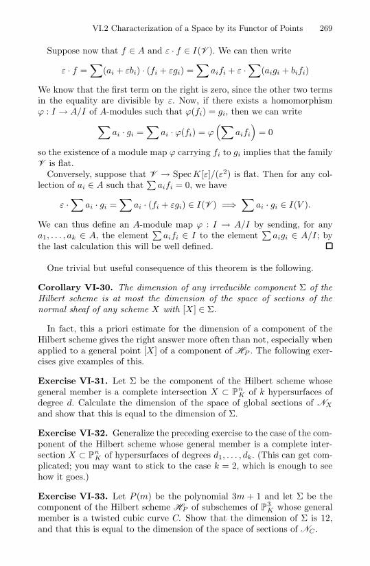
VI.2 Characterization of a Space by its Functor of Points 269
Suppose now that f ∈ A and ε · f ∈ I(V ). We can then write
ε · f =∑
(ai + εbi) · (fi + εgi) =∑
aifi + ε ·∑
(aigi + bifi)
We know that the first term on the right is zero, since the other two termsin the equality are divisible by ε. Now, if there exists a homomorphismϕ : I → A/I of A-modules such that ϕ(fi) = gi, then we can write∑
ai · gi =∑
ai · ϕ(fi) = ϕ(∑
aifi
)= 0
so the existence of a module map ϕ carrying fi to gi implies that the familyV is flat.
Conversely, suppose that V → Spec K[ε]/(ε2) is flat. Then for any col-lection of ai ∈ A such that
∑aifi = 0, we have
ε ·∑
ai · gi =∑
ai · (fi + εgi) ∈ I(V ) =⇒∑
ai · gi ∈ I(V ).
We can thus define an A-module map ϕ : I → A/I by sending, for anya1, . . . , ak ∈ A, the element
∑aifi ∈ I to the element
∑aigi ∈ A/I; by
the last calculation this will be well defined.
One trivial but useful consequence of this theorem is the following.
Corollary VI-30. The dimension of any irreducible component Σ of theHilbert scheme is at most the dimension of the space of sections of thenormal sheaf of any scheme X with [X ] ∈ Σ.
In fact, this a priori estimate for the dimension of a component of theHilbert scheme gives the right answer more often than not, especially whenapplied to a general point [X ] of a component of HP . The following exer-cises give examples of this.
Exercise VI-31. Let Σ be the component of the Hilbert scheme whosegeneral member is a complete intersection X ⊂ Pn
K of k hypersurfaces ofdegree d. Calculate the dimension of the space of global sections of NX
and show that this is equal to the dimension of Σ.
Exercise VI-32. Generalize the preceding exercise to the case of the com-ponent of the Hilbert scheme whose general member is a complete inter-section X ⊂ Pn
K of hypersurfaces of degrees d1, . . . , dk. (This can get com-plicated; you may want to stick to the case k = 2, which is enough to seehow it goes.)
Exercise VI-33. Let P (m) be the polynomial 3m + 1 and let Σ be thecomponent of the Hilbert scheme HP of subschemes of P3
K whose generalmember is a twisted cubic curve C. Show that the dimension of Σ is 12,and that this is equal to the dimension of the space of sections of NC .

270 VI. Schemes and Functors
Exercise VI-34. By way of warning, the component Σ of the precedingexercise is not the only component of the Hilbert scheme: there is anothercomponent Σ′ whose general member is the (disjoint) union of a plane cubiccurve and a point. These two intersect in the locus of schemes C ⊂ P3
K suchthat C is the union of a plane curve C0 and the double point (that is, thescheme given by the square of the maximal ideal of a point) supported ata singular point of C0. At a point of their intersection HP is singular, andits tangent space will be strictly larger than the dimension of either Σ orΣ′. Verify this.
It is not always the case, however, that the dimension of a component ofthe Hilbert scheme is equal to the dimension of the space of sections of thenormal sheaf of a general member; there are examples of Hilbert schemesthat are nonreduced along whole components, even when the general pointsof those components correspond to nonsingular, irreducible varieties. Thefirst example of this is due to Mumford [1962]; the following series of exer-cises describes it.
Mumford’s example deals with curves of degree 14 and genus 24 in pro-jective 3-space P3
K over a field K. There are (as we shall see) several compo-nents of the Hilbert scheme parametrizing such curves; we will be concernedwith the component whose general member lies on a nonsingular cubic sur-face. By way of notation, let P (m) = 14m − 23 be the Hilbert polynomialof a curve of degree 14 and genus 24, and let H be the Hilbert schemeparametrizing subschemes of P3
K with this Hilbert polynomial. We will de-note by Σ the subset of H corresponding to nonsingular curves C ⊂ P3
K ofdegree 14 and genus 24 that are contained in a nonsingular cubic surface Sand linearly equivalent on S to 4H +2L, where H is the hyperplane divisorand L a line on S.
Exercise VI-35. Show that Σ is a constructible subset of H and that itsclosure Σ in H has dimension 56.
Not all curves of degree 14 and genus 24 in P3K have to lie on cubic
surfaces. Thus, it is not a priori clear that the subvariety Σ ⊂ H is anirreducible component of H : the curves C parametrized by Σ could bespecializations of other curves not lying on cubics. To see that this is notin fact the case, we make another dimension count.
Exercise VI-36. Let C be a nonsingular, irreducible curve of degree 14and genus 24 in P3
K , and assume that C does not lie on a cubic surface.Show that it must lie on two quartic surfaces T, T ′ not having a commoncomponent, and that the residual intersection of T and T ′ (that is, theunion of the irreducible components of T ∩ T ′ other than C) is a curve ofdegree 2. By analyzing what this residual intersection may look like, showthat the set of such curves C is a constructible subset of H whose closurehas dimension at most 56. Deduce that the subvariety Σ of Exercise VI-35is indeed an irreducible component of H .

VI.2 Characterization of a Space by its Functor of Points 271
Exercise VI-37. Now let C be a nonsingular curve of degree 14 and genus24 lying on a nonsingular cubic surface S ⊂ P3
K . Using the exact sequence
0 → NC/S → NC/P3K→ NS/P3
K⊗ OC → 0
(where for any pair of schemes X ⊂ Y we write NX/Y for the normalsheaf Hom(JX/Y , OX) of X in Y ), show that the dimension of the spaceof sections of the normal sheaf NC/P3
Kis 57. Deduce that H is nowhere
reduced along Σ.
Finally, here is an amusing fact about the Hilbert scheme of rationalnormal curves, generalizing a calculation we made in Section IV.4.
Exercise VI-38. Let K be a field. For any r, let P (m) be the polyno-mial rm + 1, and let Σ be the open subset of the Hilbert scheme HP ofsubschemes of Pr
K parametrizing rational normal curves of degree r; checkthat Σ is irreducible of dimenion r2 + 2r− 3. Let C ⊂ Σ× Pr
K → Σ be theuniversal curve over Σ. Let L be the function field of Σ, and CL the fiberof C over the generic point Spec L of Σ. Show that CL
∼= P1L if and only if
r is odd.
Tangent Spaces to Fano Schemes. One particularly nice example ofschemes that are in many ways best characterized by their functor of pointsare the Fano schemes Fk(X) ⊂ GS(k, n) of a scheme X ⊂ Pn
S describedin Section IV.3. We will see, for example, how the description given inSection VI.1.3 of the tangent spaces to a functor allows us to compute theZariski tangent spaces to a Fano scheme much more readily that we couldfrom the explicit equations introduced in Section IV.3; this will in turnallow us to say in many cases whether a linear space Λ ⊂ X corresponds toa nonsingular or a singular point of Fk(X). (For the following discussion, wewill introduce some notation: for a plane W ⊂ Kn+1 and the correspondinglinear subspace Γ ⊂ Pn
K , we’ll write Γ = [W ] and W = Γ.)The characterization of Fano schemes is straightforward: we may de-
fine the Fano scheme Fk(X) of a subscheme X ⊂ PnS to be simply the
Hilbert scheme HP,X of subschemes of X with Hilbert polynomial P (m) =(k+m
k
)— that is, the functor
fk(X) : (S − schemes) −→ (sets)
that associates to any S-scheme B the set of families of k-planes containedin X ×S B, that is,
fk(X)(B) =
Σ ⊂ B ×S X ⊂ B × PnS = Pn
B, flat over B,such that Σb ⊂Pn
κ(b) is a k-plane for all b∈B
.
We then have:
Proposition VI-39. The functor fk(X) is represented by the Fano schemeFk(X) introduced in Section IV.3.

272 VI. Schemes and Functors
Proof. To establish this, we have to exhibit an isomorphism of functors
fk(X)(B) −→ MorS(B, Fk(X)),
that is, for any S-scheme B a natural bijection between two sets, the setof families Σ ⊂ B ×S X ⊂ B × Pn
S = PnB of k-planes contained in X
and morphisms from B to Fk(X) as S-schemes. In fact, the serious workhas already been done: the definition of the map and the proof that itis a bijection are not hard, given that we have already characterized theGrassmannian GS(k, n) as the scheme representing the functor of familiesof k-planes in Pn
S .The point is, we already have an isomorphism of functors
gS(n+1, k+1) −→ MorS(B, GS(k+1, n+1))
where gS(n+1, k+1) is the Grassmannian functor introduced in SectionVI.2.1, here in the category of S-schemes. That is, we associate to anyfamily Σ ⊂ B × Pn
S = PnB , flat over B with k-plane fibers, a morphism
ϕΣ : B → GS(k, n) over S. Now all we need to check is that the subsetfk(X)(B) ⊂ g(n+1, k+1)(B) is carried into the subset MorS(B, Fk(X)) ⊂MorS(B, GS(k+1, n+1)), that is, that
Σ ⊂ B ×S X ⊂ B × PnS ⇐⇒ ϕΣ(B) ⊂ Fk(X) ⊂ GS(k+1, n+1).
This is immediate, given the description in Section IV.3 of the definingequations of Fk(X).
As promised, the characterization of the Fano scheme by its functor ofpoints allows us to determine its tangent spaces readily, and in particularto give us criteria for the smoothness and/or singularity of Fano schemes.
For the following, then, K will be an algebraically closed field, X ⊂ PnK
will be an arbitrary projective scheme over K, Fk(X) ⊂ GK(k+1, n+1)the Fano scheme of k-planes contained in X and Λ ∈ Fk(X) a K-valuedpoint of Fk(X). Write ∆ for the scheme Spec K[ε]/(ε2) and 0 ∈ ∆ for thereduced point ∆red
∼= Spec K ⊂ ∆. According to our characterization ofFk(X) as the scheme representing the functor of families of k-planes on X,the tangent space to Fk(X) at the point Λ will be
TΛ(Fk(X)) =
subschemes Σ ⊂ ∆ ×K X flat over ∆such that Σ ∩ (0 ×K X) = Λ
.
We will now see how to describe this as a subspace of
TΛ(GK(k + 1, n + 1)) = Hom(Λ, Kn+1/Λ).
Probably the fastest way to do this is simply to observe that a first-orderdeformation of a plane Λ ⊂ Pn
K — that is, a subscheme Σ ⊂ ∆ ×K PnK
flat over ∆ and such that Σ ∩ (0 ×K X) = Λ— is the union of its tangentvectors, viewed as subschemes of Σ isomorphic to ∆. In other words, Σwill be contained in a subscheme ∆×K X ⊂ ∆×K Pn
K if and only if everytangent vector to Σ is a tangent vector to ∆ ×K X.

VI.2 Characterization of a Space by its Functor of Points 273
Now, suppose that the first-order deformation Σ of a plane Λ correspondsto a homomorphism ϕ : Λ → Kn+1/Λ. The tangent vectors to Σ at a pointp (more properly, 0 ×K p) will then be the tangent vectors to ∆ ×K Pn
K
corresponding to homomorphisms ν : p → Kn+1/p such that
ν(p) ⊂ ϕ(Λ).
Similary, to say that the tangent vector corresponding to such a homomor-phism ν is tangent to ∆ ×K X is to say that
ν(p) ⊂ TpX + Λ.
Thus, to say that the tangent vector to the Grassmannian associated tothe homomorphism ϕ lies in the tangent space to the Fano scheme Fk(X)at Λ is to say that the image of ϕ is contained in the tangent space to Xat each point, i.e.,
TΛ(Fk(X)) =
ϕ ∈ Hom(p, Kn+1/Λ) such thatϕ(v) ∈ TpX + Λ for all v ∈ Λ
.
As an application, consider the simplest possible case, the Fano schemeF1(S) ⊂ GK(1, 3) = GK(2, 4) of lines on a surface S ⊂ P3
K . Let L ⊂ Sbe a line, which we will assume is not contained in the singular locus of S(if it is, the Fano scheme F1(S) will have four-dimensional tangent spaceat L —in other words, it will be very singular!). To a general point p ∈ L,then, we may associate the projective tangent space TpS, which will be aplane in P3
K containing L; thus we get a (rational) map
γ : L −→ P(K4/L) ∼= P1K .
This map is given by the partial derivatives of the defining polynomial of S,so that if S is nonsingular along L —in other words, if these partials haveno common zeroes— the degree of γ will be d − 1. If S has any singularpoints on L, conversely, it will be less.
In fact, the degree of the map γ is precisely what determines the di-mension of the tangent space to F1(S) at L. This is simple to see: ifϕ : L → K4/L is any homomorphism, the induced map
ϕ : L −→ P(K4/L) ∼= P1K
p −→ [ϕ(p) + L]
will have degree 1 if ϕ has rank 2 and degree 0 if ϕ has rank 1. Thus,if γ has degree deg(γ) ≥ 2, the tangent space to F1(S) at L will be zero-dimensional; if γ has degree 1 it will be one-dimensional; and if γ is constantit will be two-dimensional. We get the following corollaries:
• The Fano scheme of lines on a nonsingular quadric surface in P3K is
nonsingular, while the Fano scheme of lines on a quadric cone is every-where nonreduced.

274 VI. Schemes and Functors
• More generally, the Fano scheme of the cone in P3K over any plane
curve is nonreduced.
• The Fano scheme of lines on a nonsingular surface of degree d ≥ 3 inP3
K consists of isolated reduced points.
There is a further corollary dependent on a further fact about Fanoschemes of hypersurfaces: if X ⊂ Pn
B is any hypersurface of degree d—thatis, a closed subscheme of Pn
B, flat over S, whose fiber over each point b ∈ Bis a hypersurface of degree d in Pn
κ(b) — then the Fano scheme Fk(X) ⊂GB(k + 1, n + 1) of k-planes on X is flat over the open subset of B whereit has the expected fiber dimension (k + 1)(n − k) − (
k+dk
). Since Fk(X)
may be described as the zero locus of a section of a locally free sheaf onGB(k n), this is a generalization of the fact that complete intersections areflat, but it is beyond the scope of this book. Given it, however, we have thefollowing consequence:
• All cubic surfaces that contain only finitely many lines contain thesame number of lines, properly counted; that is, their Fano schemes allhave degree 27.
In general, our description of the tangent spaces to the Fano schemeFk(X) allows us to determine the dimension of Fk(X) at a point Λ interms of the normal bundle to the plane Λ ⊂ X, but it is rare that this willbe determined by the singularities of X along Λ. In fact, as soon as we getto hypersurfaces X ⊂ Pn
K with n ≥ 4, we see examples to the contrary.
Exercise VI-40. Use this characterization of the tangent spaces to Fanoschemes to give an example of a nonsingular hypersurface X ⊂ Pn
K suchthat the Fano scheme F1(X) of lines on X is singular.
VI.2.4 Moduli Spaces
A similar situation arises when we want to construct a moduli space ofgeometric objects. For example, we would like to identify the set of non-singular, projective curves of genus g over a field K with the set of closedpoints of a “moduli scheme” Mg. To avoid unnecessary complication, werestrict to the case char(K) = 0. Again, the way to express what we wantis to introduce the functor of nonsingular curves of genus g: this is thefunctor
M fung : (K − schemes) → (sets)
that assigns to any scheme B over K the set of flat morphisms π : X → Bwhose fibers are nonsingular curves of genus g, up to isomorphism X ∼= X ′
as B-schemes. We define Mg to be the scheme (if any) that represents thefunctor M fun
g .Since schemes are uniquely determined by their functors of points, the
only difficulty with the “definitions” above is whether such schemes exist —

VI.2 Characterization of a Space by its Functor of Points 275
that is, whether the given functors are representable. The answer in the caseof HP is yes; and indeed, as we have pointed out, the characterization ofHP as the scheme that represents the functor hP is crucial to the proof ofexistence.
However, in the case of Mg, the answer is no! For example, even in thecase of nonsingular curves of genus 1 over C there does not exist a modulispace M1 in this sense. To see this, it suffices to show that there does notexist a universal family — in other words, a flat morphism π : C → M ofschemes with fiber nonsingular curves of genus 1 such that for every familyY → B of nonsingular curves of genus 1 there are unique maps ϕ : B → Mand Φ : Y → C forming a fiber product diagram:
YΦ C
B
η ϕ M
π
In fact, there does not even exist a tautological family —that is, a morphismC → M and a bijection between the closed points of M and the set ofisomorphism classes of nonsingular curves of genus 1 such that the fiberover each point p ∈ M is in the isomorphism class corresponding to thepoint p. We will exhibit two kinds of obstructions to the existence of auniversal family, one local and one global.
For the local obstruction, recall that curves of genus 1 over C are classifiedby their j-invariant: we can write any such curve as the plane cubic
y2 = x(x − 1)(x − λ)
for some complex λ = 0, 1; and two such curves Cλ and Cλ′ will be iso-morphic if and only if their j-invariants j(λ) and j(λ′) are equal, where
j(λ) = 256 · (λ2 − λ + 1)3
λ2 (λ − 1)2;
see Silverman [1986, Chapter III, Proposition 1.7], for example. It can beshown that given a family X → B of nonsingular curves of genus 1 withnonsingular base B, the function j is a regular function on B; and locallyaround any point b ∈ B, λ can be defined as a regular function, too (thoughit is not unique). It follows that if there did exist a tautological family, therewould have to exist one with base the affine line A1
C with coordinate j. Butno such family can exist, because at the point j = 0 the function λ2 −λ+1 would vanish, and thus j would vanish triply. Less obviously, becausej′(−1) = 0, it also follows that j can only assume the value 1728 with evenmultiplicity. (Note that the values j = 0 and 1728 correspond to the ellipticcurves with “extra automorphisms”— that is, whose automorphism groupscontain the automorphism group of a general elliptic curve as subgroups ofindex 3 and 2, respectively.)
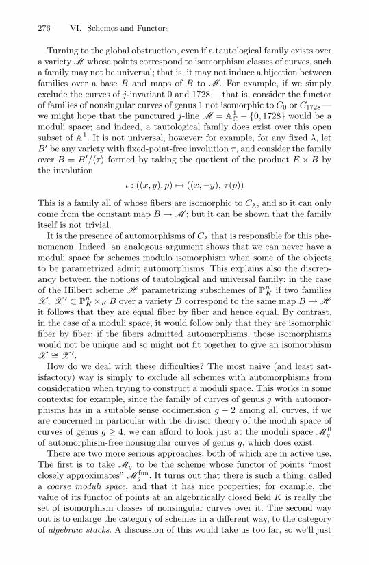
276 VI. Schemes and Functors
Turning to the global obstruction, even if a tautological family exists overa variety M whose points correspond to isomorphism classes of curves, sucha family may not be universal; that is, it may not induce a bijection betweenfamilies over a base B and maps of B to M. For example, if we simplyexclude the curves of j-invariant 0 and 1728— that is, consider the functorof families of nonsingular curves of genus 1 not isomorphic to C0 or C1728 —we might hope that the punctured j-line M = A1
C − 0, 1728 would be amoduli space; and indeed, a tautological family does exist over this opensubset of A1. It is not universal, however: for example, for any fixed λ, letB′ be any variety with fixed-point-free involution τ , and consider the familyover B = B′/〈τ〉 formed by taking the quotient of the product E × B bythe involution
ι : ((x, y), p) → ((x,−y), τ(p))
This is a family all of whose fibers are isomorphic to Cλ, and so it can onlycome from the constant map B → M ; but it can be shown that the familyitself is not trivial.
It is the presence of automorphisms of Cλ that is responsible for this phe-nomenon. Indeed, an analogous argument shows that we can never have amoduli space for schemes modulo isomorphism when some of the objectsto be parametrized admit automorphisms. This explains also the discrep-ancy between the notions of tautological and universal family: in the caseof the Hilbert scheme H parametrizing subschemes of Pn
K if two familiesX , X ′ ⊂ Pn
K ×K B over a variety B correspond to the same map B → Hit follows that they are equal fiber by fiber and hence equal. By contrast,in the case of a moduli space, it would follow only that they are isomorphicfiber by fiber; if the fibers admitted automorphisms, those isomorphismswould not be unique and so might not fit together to give an isomorphismX ∼= X ′.
How do we deal with these difficulties? The most naive (and least sat-isfactory) way is simply to exclude all schemes with automorphisms fromconsideration when trying to construct a moduli space. This works in somecontexts: for example, since the family of curves of genus g with automor-phisms has in a suitable sense codimension g − 2 among all curves, if weare concerned in particular with the divisor theory of the moduli space ofcurves of genus g ≥ 4, we can afford to look just at the moduli space M 0
g
of automorphism-free nonsingular curves of genus g, which does exist.There are two more serious approaches, both of which are in active use.
The first is to take Mg to be the scheme whose functor of points “mostclosely approximates” M fun
g . It turns out that there is such a thing, calleda coarse moduli space, and that it has nice properties; for example, thevalue of its functor of points at an algebraically closed field K is really theset of isomorphism classes of nonsingular curves over it. The second wayout is to enlarge the category of schemes in a different way, to the categoryof algebraic stacks. A discussion of this would take us too far, so we’ll just

VI.2 Characterization of a Space by its Functor of Points 277
refer the reader to Vistoli [1989, Appendix] for a short treatment and toBehrend et al. [≥ 2001] for a full treatment; see also Mumford [1965] foran introduction to the functorial point of view on moduli spaces.
References
A. Altman and S. Kleiman, Introduction to Grothendieck duality theory,Lecture Notes in Mathematics 146, Springer, Berlin, 1970.
M. Artin, Algebraic spaces, Yale Mathematical Monographs 3, Yale Uni-versity Press, New Haven, CT, 1971.
M. F. Atiyah and I. G. Macdonald, Introduction to commutative algebra,Addison-Wesley, Reading, MA, 1969.
D. Bayer and D. Eisenbud, “Ribbons and their canonical embeddings”,Trans. Amer. Math. Soc. 347:3 (1995), 719–756.
K. Behrend, L. Fantechi, W. Fulton, L. Gottsche, and A. Kresch, “In-troduction to stacks”. In preparation.
E. Bombieri and D. Mumford, “Enriques’ classification of surfaces inchar. p, III”, Invent. Math. 35 (1976), 197–232.
N. Bourbaki, Commutative algebra, Chapters 1-7, Hermann, Paris, 1972.Reprinted by Springer, New York, 1989.
E. Brieskorn and H. Knorrer, Plane algebraic curves, Birkhauser, Basel,1986.
J. W. S. Cassels and A. Frohlich (editors), Algebraic number theory(Brighton, 1965), Academic Press, London, 1967. Reprinted 1986.
H. Clemens, J. Kollar, and S. Mori, Higher-dimensional complex geome-try, Asterisque 166, Soc. math. France, Paris, 1988.

280 References
A. Collino, “Evidence for a conjecture of Ellingsrud and Strømme onthe Chow ring of HilbdP2
C”, Illinois Journal of Mathematics 32 (1988),171–210.
J. L. Coolidge, A treatise on algebraic plane curves, Oxford UniversityPress, 1931.
D. Cox, J. Little, and D. O’Shea, Ideals, varieties, and algorithms, Sec-ond ed., Springer, New York, 1997. An introduction to computationalalgebraic geometry and commutative algebra.
P. Deligne, “La conjecture de Weil, I”, Inst. Hautes Etudes Sci. Publ.Math. 43 (1974), 273–307.
M. Demazure and P. Gabriel, Groupes algebriques, I: Geometrie alge-brique, generalites, groupes commutatifs, Masson, Paris, 1970.
D. Eisenbud, Commutative algebra with a view toward algebraic geome-try, Graduate Texts in Mathematics 150, Springer, New York, 1995.
G. Faltings, “Die Vermutungen von Tate und Mordell”, Jahresber.Deutsch. Math.-Verein. 86:1 (1984), 1–13.
L.-Y. Fong, “Rational ribbons and deformation of hyperelliptic curves”,J. Algebraic Geom. 2:2 (1993), 295–307.
O. Forster, Lectures on Riemann surfaces, Graduate Texts in Mathemat-ics 81, Springer, New York, 1981. Translated from the German by BruceGilligan.
W. Fulton, Intersection theory, vol. 2, Ergebnisse der Mathematik undihrer Grenzgebiete (3), Springer, Berlin, 1984.
R. Godement, Topologie algebrique et theorie des faisceaux, Actualit’esSci. Ind. 1252, Hermann, Paris, 1964.
M. L. Green, “Koszul cohomology and the geometry of projective vari-eties”, J. Differential Geom. 19:1 (1984), 125–171. with an appendix byM. Green and R. Lazarsfeld.
M. Green and R. Lazarsfeld, “On the projective normality of completelinear series on an algebraic curve”, Invent. Math. 83:1 (1985), 73–90.
P. Griffiths and J. Harris, Principles of algebraic geometry, Wiley-Interscience, New York, 1978. Reprinted 1994.
A. Grothendieck, “Elements de geometrie algebrique, I: Le langage desschemas”, Inst. Hautes Etudes Sci. Publ. Math. 4 (1960), 1–228.
A. Grothendieck, “Elements de geometrie algebrique, II: Etude globaleelementaire de quelques classes de morphismes”, Inst. Hautes Etudes Sci.Publ. Math. 8 (1961), 1–222.
A. Grothendieck, “Elements de geometrie algebrique, III: Etude co-homologique des faisceaux coherents (premiere partie)”, Inst. HautesEtudes Sci. Publ. Math. 11 (1961), 1–167.

References 281
A. Grothendieck, “Elements de geometrie algebrique, III: Etude coho-mologique des faisceaux coherents (seconde partie)”, Inst. Hautes EtudesSci. Publ. Math. 17 (1963), 1–91.
A. Grothendieck, “Elements de geometrie algebrique, IV: Etude localedes schemas et des morphismes de schemas (premiere partie)”, Inst.Hautes Etudes Sci. Publ. Math. 20 (1964), 1–259.
A. Grothendieck, “Elements de geometrie algebrique, IV: Etude localedes schemas et des morphismes de schemas (seconde partie)”, Inst.Hautes Etudes Sci. Publ. Math. 24 (1965), 1–231.
A. Grothendieck, “Elements de geometrie algebrique, IV: Etude localedes schemas et de morphismes de schemas (troisieme partie)”, Inst.Hautes Etudes Sci. Publ. Math. 28 (1966), 1–255.
A. Grothendieck, “Elements de geometrie algebrique, IV: Etude localedes schemas et des morphismes de schemas (quatrieme partie)”, Inst.Hautes Etudes Sci. Publ. Math. 32 (1967), 1–361.
R. C. Gunning, Introduction to holomorphic functions of several vari-ables, III: Homological theory, Wadsworth and Brooks/Cole, Monterey,CA, 1990.
J. Harris, “Galois groups of enumerative problems”, Duke Math. J. 46:4(1979), 685–724.
J. Harris, Algebraic geometry: A first course, Graduate Texts in Math.133, Springer, New York, 1995. Corrected reprint of the 1992 original.
J. Harris and D. Eisenbud, Curves in projective space, Les Presses del’Universite de Montreal, Montreal, 1982.
J. Harris and I. Morrison, Moduli of curves, Graduate Texts in Mathe-matics 187, Springer, New York, 1998.
R. Hartshorne, Algebraic geometry, Graduate Texts in Mathematics 52,Springer, New York, 1977.
D. Hilbert, “Uber die theorie der algebraischen formen”, MathematischeAnnalen 36 (1890), 473–534.
H. Hironaka, “An example of a non-Kahlerian deformation”, Annals ofMathematics 75 (1962), 190–208.
A. Iarrobino, “Compressed algebras and components of the punctualHilbert scheme”, pp. 146–165 in Algebraic geometry (Sitges, Barcelona,1983), edited by E. Casas-Alvero, Lecture Notes in Math. 1124, Springer,Berlin, 1985.
G. Kempf, F. F. Knudsen, D. Mumford, and B. Saint-Donat, Toroidalembeddings, I, Lecture Notes in Mathematics 339, Springer, Berlin, 1973.
S. Kleiman, “Misconceptions about KX”, Enseign. Math. 25 (1979),203–206.

282 References
D. Knutson, Algebraic spaces, Lecture Notes in Math. 203, Springer,Berlin, 1971.
J. Kollar, “The structure of algebraic threefolds: an introduction toMori’s program”, Bull. Amer. Math. Soc. (N.S.) 17:2 (1987), 211–273.
J. Kollar, Rational curves on algebraic varieties, Ergebnisse der Mathe-matik, 3. Folge 32, Springer, Berlin, 1996.
S. Lang, Algebraic number theory, 2nd ed., Graduate Texts in Math. 110,Springer, New York, 1994.
H. Matsumura, Commutative ring theory, Cambridge University Press,Cambridge, 1986. Second edition, 1989.
D. Mumford, “Further pathologies in algebraic geometry”, Amer. J.Math. 84 (1962), 642–648.
D. Mumford, “Picard groups of moduli problems”, pp. 33–81 in Arith-metical Algebraic Geometry (Purdue Univ., 1963), edited by O. F. G.Schilling, Harper & Row, New York, 1965.
D. Mumford, Lectures on curves on an algebraic surface, Annals of Math-ematics Studies 59, Princeton University Press, Princeton, 1966.
D. Mumford, Algebraic geometry I : complex projective varieties,Grundlehren der mathematischen Wissenschaften 221, Springer, Berlinand New York, 1976.
D. Mumford, The red book of varieties and schemes, Lecture Notes inMath. 1358, Springer, Berlin, 1988.
M. Nagata, Local rings, Tracts in Pure and Applied Mathematics 13,Wiley/Interscience, New York and London, 1962.
D. G. Northcott, Ideal theory, Cambridge Tracts in Mathematics andMathematical Physics 42, University Press, Cambridge, 1953.
M. Raynaud and L. Gruson, “Criteres de platitude et de projectivite.Techniques de “platification” d’un module”, Invent. Math. 13 (1971),1–89.
M. Reid, Undergraduate algebraic geometry, London Mathematical Soci-ety Student Texts 12, Cambridge University Press, Cambridge and NewYork, 1988.
B. Segre, The nonsingular cubic surfaces, Oxford Univ. Press, 1942.
J.-P. Serre, “Faisceaux algebriques coherents”, Ann. of Math. (2) 61(1955), 197–278.
J.-P. Serre, Groupes algebriques et corps de classes, 2nd ed., Hermann,Paris, 1975. Translated as Algebraic groups and class fields, Graduatetexts in mathematics 117, Springer, New York, 1988.
J.-P. Serre, Local fields, Springer, New York, 1979.

References 283
I. R. Shafarevich, Basic algebraic geometry, vol. 213, Die Grundlehrender mathematischen Wissenschaften, Springer, New York, 1974. Secondedition (in two volumes), 1994.
J. H. Silverman, The arithmetic of elliptic curves, Springer, New York,1986.
E. H. Spanier, Algebraic topology, McGraw-Hill, New York, 1966.
R. G. Swan, Theory of sheaves, Chicago Lectures in Mathematics, Uni-versity of Chicago Press, Chicago, 1964.
A. Vistoli, “Intersection theory on algebraic stacks and on their modulispaces”, Invent. Math. 97:3 (1989), 613–670.
W. Vogel, Lectures on results on Bezout’s theorem, Lectures on mathe-matics and physics 74, Tata Institute of Fundamental Research, Bombay,and Springer, Berlin, 1984. Notes by D. P. Patil.
R. J. Walker, Algebraic Curves, Princeton Mathematical Series 13,Princeton University Press, Princeton, NJ, 1950. Reprinted by Dover,1962, and Springer, 1978.
O. Zariski, “The concept of a simple point of an abstract algebraic vari-ety”, Trans. Amer. Math. Soc. 62 (1947), 1–52.

Index
A2 singularity, 204absolutely irreducible, 56acnode, 57affine
line, 48locally, 21pair, 22plane, 48scheme, 7, 8, 21, 30
–s and commutative rings, 36primary, 68
space, 33, 34, 47, 84tangent space, 104, 105variety, 47
algebraAzumaya, 206category of –s, 253, 258coordinate, 28, 47dimension of, 32, 60division, 207graded, 91, 95, 100, 101, 170Noetherian, 81quasicoherent sheaf of –s, 40, 101reduced, 47, 53Rees, 172, 173spectrum of, 40, 111symmetric, 102, 105, 122, 173tensor product of –s, 37
algebraic
geometry, see classicalspaces, 262stack, 276
algebraically closed, 8–11, 47, 48,50, 58, 62, 65, 83, 104, 119, 123,140, 141, 151, 153–156, 160, 163,178, 191–193, 195, 203, 207, 213,228, 231, 239, 243, 245, 248, 272,276
Alonso, Leo, 5Altman, Allen, 230analytic
branch, 52functions, 27functions, sheaf of, 14manifold, 8, 51spaces, 116
annihilator sheaf, 220arithmetic
genus, 129, 138scheme, 81, 110, 162, 180, 185,
188, 245, 249Artin, Michael, 53, 261Artinian ring, 65, 78associated
closed ideal, 100prime, 67scheme, 68to a variety, 47

286 Index
axiom of choice, 12Azumaya algebra, 206
Bezout’s theorem, 141, 146, 148,154
basechange, 38, 54, 152, 154, 168,
209, 213, 216, 219, 221, 222,236, 237, 241
Grobner, 75of open sets, 16scheme, 45, 95, 122, 193, 222
basic open set, 10, 14, 16, 30Bayer, David, 138Behrend, Kai A., 277Betti number, 127, 128, 130blow-up, 103, 162–192Bombieri, Enrico, 1Bourbaki, Nicolas, 76, 112Brauer group, 206Brieskorn, Egbert, 52Brill–Noether–Petri problems, 1Brown, Edgar H., 261Buhler, Joe, 5Burch, Lindsay, 133
Cartierdivisor, 110, 117, 166, 167, 174subscheme, 165, 167, 168, 175,
176, 178, 182Cassels, J. W. S., 206Castelnuovo regularity, 264categorical
definitionof morphism of sheaves, 15of presheaf, 12
equivalence of affine schemesand rings, 30
category, opposite, 30center of blow-up, 165Chevalley, Claude, 210Chinese Remainder Theorem, 60choice, axiom of, 12
classicalalgebraic geometry, 8, 9, 28, 34,
40, 47, 49, 57, 59, 94, 109, 114,117, 119, 120, 125, 138, 140,141, 148, 151–154, 156,161–165, 180, 184, 192, 193,197, 210, 222–224, 231–233,240, 242, 246–248
Clemens, Herbert, 5, 179closed
locally, 26point, 11, 22, 26, 31, 42, 48,
50–52, 54–56, 60, 63, 70, 71,75, 76, 82, 83, 85, 88, 93, 105,111, 132, 160, 191, 216, 239,247, 255, 256, 274, 275
subfunctor, 255subscheme, 23, 24, 71, 100, 211universally, 95
closure, 26coarse moduli space, 276Cohen–Macaulay, 32, 146, 151coherent sheaf, 24, 25, 103cokernel, 16Collino, Alberto, 265commutative ring, see ringcompactness, 19, 91, 93–95, 229compatibility condition, 33complex, see also analytic
manifold, 8, 20component
embedded, 66, 68isolated, 67, 68length of, 68multiple, 156primary, 67, 68
conecubic, 63over a cubic, 204over a quartic, 148quadric, 173, 175, 197–199tangent, 106–110, 171, 178, 190,
192, 203, 204projectivized, 107

Index 287
conic, 63, 86, 141, 142, 160, 179,185, 186, 190, 196, 198, 202and quartic, 160double, 138, 156, 157intersection of –s, 143intersection with line, 59reducible and nonsingular, 87universal, 207, 208
constructiblesubset, 209
containment of schemes, 23continuous
functions, sheaf of, 13Coolidge, Julian L., 152, 242coordinate ring, 47cotangent
sheafrelative, 231
sheaf, relative, 230space, Zariski, 27
Cox, David, 229crunode, 57cubic
lines on, 202surface, 191universal, 203, 204
curvilinearscheme, 65
cusp, 156, 239
decomposition, primary, 67, 68Dedekind domain, 71, 75deformation, first-order, 267degree
of affine scheme, 62, 65of scheme, 129, 141of subscheme, 125
dehomogenization, 98, 153Deligne, Pierre, 1Demazure, Michel, 261diagonal subscheme, 93Dieudonne, Jean, 5different of a polynomial, 234dimension
Krull, 27, 65
of scheme, 27relative, 231
direct limit, 14discriminant
of a polynomial, 233scheme, 231
distinguished open set, 10, 23division algebra, 207divisor
Cartier, 117exceptional, 164, 165
dominant morphism, 211double
conic, 138line, 136point, 58, 62, 88, 178, 180, 246
dualcurve, 162, 237, 240projective space, 103
effective Cartier divisor, 117elemination theory, 210Eliot, Thomas Stearns, velliptic curve, 161embedded
component, 66, 68point, 66
equalizer, 35equations with parameters, 70etale
equivalence relations, 262topology, 53
Euler’s relation, 153exceptional divisor, 164, 165
faithful functor, 43Faltings, Gerd, 1family
flat, 75limit of, 71of closed subschemes, 71of curves, 156of schemes, 70universal, 222
Fano

288 Index
scheme, 120, 193–205, 266, 273tangent space to, 271universal, 203
variety, universal, 204Fantechi, L., 277fiber, 31, 38, 49, 70fibered
coproduct, 37product, 35, 36, 254, 260sum, 37
finitemorphism, 92scheme, 62type, 76, 210, 231type, morphism of, 92
finitely generated, 8, 47, 50first-order
deformation, 267neighborhood, 58, 67
Fitting’s Lemma, 219ideal, 220, 221, 225, 231, 232,
236, 238image, 219, 221–224scheme, 220
flatfamily, 75, 125limit, 77module, 75scheme, 32
flatnessgeometric interpretation of, 125theorem, 79
flex, 151, 152flop, 179Fong, Lung-Ying, 138form (type of scheme), 205Forster, Otto, 18Four Quartets, vfree resolution, 127, 128, 133, 134,
144Frobenius automorphism, 56Frohlich, Albrecht, 206Fulton, William, 148, 277functor
faithful, 43injective, 254of nonsingular curves, 274of points, 42, 43, 252representable, 44tangent space to, 256
Gottsche, Lothar, 277Gabriel, Pierre, 261Galois
cohomology, 206group, 40, 56, 85, 87
Gashorov, Vesselin, 5Gathmann, Andreas, 5generic
flatness theorem, 79hypersurface, 123point, 9, 48
genus, arithmetic, 129, 138geometrically irreducible, 56germ
of analytic function, 14of variety, 50
globalProj, 102, 170regular function, 22section, 12Spec, 40, 41
gluing, 33Godement, Roger, 18Grobner bases, 75, 229Graber, Tom, 5graded
algebra, 91, 95, 100, 101, 170Betti number, 127Betti numbers, 128, 130module, 118ring, Proj of, 95sheaf, 118
grading, 34, 96Grassmannian, 63, 119, 193, 195,
201, 206, 207, 261, 263, 264, 272,273functor, 261
Green, Mark L., 130

Index 289
Griffiths, Phillip, 1, 155, 192, 203Gross, Benedict, 5Grothendieck, Alexandre, 1, 5, 18,
79, 261group scheme, 258Gruson, Laurent, 77Gunning, Robert C., 18
Hartshorne, Robin, 4, 5, 18, 75,95, 101, 110, 125, 126, 129, 155,162, 210, 218
Hassett, Brendan, 5Hausdorff, 11, 19, 91, 93, 95Henselization, 52Hessian, 153–155, 157Hilbert
David, 48, 125, 128function, 124–130functor, 262polynomial, 125, 129, 130, 143,
262–264scheme, 120, 129, 259, 262, 264,
266tangent space to, 267
series, 149, 150Theorem, 125theorems, 128
Hironaka, Heisuke, 261homogeneous
coordinate ring, 96element, 96ideal, 96
homogenization, 98hyperplane, universal, 124hypersurface, 122, 141
generic, 123universal, 123
Iarrobino, Anthony, 64, 265ideal, see prime, maximal,
minimalFitting, 220, 221, 225, 231, 232,
236, 238of minors, 219sheaf, 24
imageFitting, 219, 221–224of morphism, 209reduced, 222scheme-theoretic, 222, 223set-theoretic, 209, 222
infinitely near point, 59injective functor, 254intersection
multiplicity, 141, 148, 151of schemes, 24
invariance under base change, 209j-invariant, 185, 205, 275, 276invariants of projective scheme,
124inverse
image, see preimagelimit, 17, 53of a sheaf, 117
invertiblemodule, 113sheaf, 112, 116, 117
irreducible scheme, 25absolutely, 56
irrelevant ideal, 96isolated component, 67, 68
j-function, 184j-invariant, 185, 205, 275, 276Jacobian, 230, 231Jeremias, Ana, 5join, 147
Kahler differentials, 230Kempf, George R., 33Kleiman, Steven, 118, 230Knutson, Donald, 262Knorrer, Horst, 52Kollar, Janos, 1, 179, 263Koszul complex, 143, 144, 173Kresch, A., 277Krull dimension, 27, 39, 65Krull, Wolfgang, 28
Lang, Serge, 234

290 Index
Lazarsfeld, Robert, 130leading term, 107Lee, Alex, 5Lefschetz Hyperplane Theorem,
124length
of component, 68of module, 68of ring, 66of scheme, 66
Levy, Silvio, 5Lie group, 161limit
direct, 14flat, 77inverse, 17, 53of one-parameter family of
schemes, 71“Little Gidding”, vLittle, John, 229local
homomorphism, 30ring, 30, 51, 65
of a scheme, 22, 27ringed space, 22scheme, 50
locallyaffine, 21closed subscheme, 26complete intersection
subschemes, 146free module, 112induced, 16Noetherian, 253
manifold, 8map, see morphismMatsumura, Hideyuki, 75–77, 79,
128maximal
ideal, 9–11, 27, 30, 31Mederer, Kurt, 5minimal prime, 25, 26minors, ideal of, 219module
flat, 75length of, 68presheaf of –s, 12
moduli space, 274, 276monodromy group, 143Mordell, conjecture, 1Mori, Shigefumi, 1, 179morphism
dominant, 211image of, 209of schemes, 28, 29of schemes over S, 40of sheaves, 15projective, 97, 101proper, 95to projective space, 110
S-morphism, 40Morrison, David, 1multiple
component, 242components, 156line, 80point, 62, 182
multiplicity, 107intersection, 151of a flex, 154of associated scheme, 68of intersection, 141of point, 60of ring, 66of scheme, 65, 66
Mumford, David, 1, 5, 78, 192,263, 270, 277
Mustata, Mircea, 5
Nagata, Masayoshi, 56Nakayama’s Lemma, 62, 126, 128,
166, 171, 217, 218Nash manifold, 8nilpotent-free, see also reduced, 8nilradical
of a ring, 25of a scheme, 25
node, 57, 156, 239Noetherian

Index 291
algebra, 81ring, 19, 26, 28, 67, 130, 172, 253scheme, 26–28, 183, 210, 231
nonaffine scheme, 22, 33nonalgebraically closed, 53, 57, 65,
84, 142, 152, 191, 193, 195, 201,241
nonclosed point, 42, 48, 51, 56, 85,87, 114
nonreduced scheme, 57, 180nonsingular
curves, functor of, 274scheme, 28
normal sheaf, 268Northcott, D. G., 67Nullstellensatz, 48, 54number field, 82
O’Shea, Donal, 229Ogus, Arthur, 5open
covering, of a functor, 255subfunctor, 254subscheme, 23
opposite category, 30order (in a number field), 84, 188ordinary
double point, 178node or tacnode, 239
over K, scheme, 39over something
scheme, 40
parameter spaces, 262parameters, equations with, 70Pardue, Keith, 5partition of unity, 20Peeva, Irena, 5Pell’s equation, 205pencil
of cubics, 184, 204of plane curves, 185of quadrics, 201
Pluckercoordinates, 207
equations, 120, 121formulas, 156, 242ideal, 122relations, 121
plane curve, 123, 152power series, 14, 52, 53, 71preimage, 31, 38, 49, 52presheaf, 11primary
affine scheme, 68component, 67, 68decomposition, 67, 68ideal, 67
prime, 9associated, 67ideal sheaf, 41minimal, 25
product, fibered, 35, 254Proj, 170
global, 102of graded ring, 95
projectivebundle, 103module, 113morphism, 97, 101scheme, 91, 95
invariants of, 124space, 34, 35, 96
dual, 103space, morphisms to, 110tangent, 152tangent space, 104, 105
projectivization, 103of coherent sheaf, 103
propermap of Hausdorff spaces, 95morphism, 95transform, 168
properness, 19pullback, 35push-pull property, 209, 210pushforward, 18
quadratic form, 53quadric

292 Index
cone, 197–199degeneration, 199lines on, 195surface, 191universal, 202
quasicoherent sheaf, 24, 25of OS-algebras, 40of graded algebras, 101
quasicompactness, 19, 93quaternions, 206
radical, 67ramification, 83rational
function, 20, 52over K, 45, 256
Raynaud, Michel, 77reduced
algebra, 47, 50, 53image, 222ring, 26scheme, 25, 47, 53, 68
Rees algebra, 172, 173regular
function, 10, 22global, 22sheaf of –s, 9, 11, 19
scheme, 28section, 117subscheme, 165, 172
regularity, 251Reid, Miles, 5relative
cotangent sheaf, 230, 231dimension, 231Hilbert scheme, 266scheme, 35
relevant ideal, 96representable
functor, 44scheme, 252
residue field, 9resolution
free, 127, 128, 133, 134small, 179
restriction, 11, 13resultant, 213, 219, 222–224Riemann
sphere, 15surface, 83, 129
ring, 8–s and affine schemes, 36Artinian, 65, 78category of –s, 30homomorphism and morphism
of affine schemes, 30length of, 66local, 51, 65map of, 30multiplicity of, 66Noetherian, 26, 67, 172of integers in a number field, 82spectrum of, 9
ring (i.e., commutative ring withidentity), 7
ringed space, 21, 22
Samuel, Pierre, 125saturation, 101scheme
affine, 7, 8, 21, 30primary, 68
arithmetic, 81, 110, 162, 180,185, 188, 245, 249
as a set, 9as a topological space, 10associated, 68associated to vector space, 105containment of –s, 23curvilinear, 65degree of, 62, 65dimension of –s, 27discriminant, 231family of –s, 70Fano, 120, 193–205, 266, 273finite, 62Fitting, 220general definition of, 21group, 258Hilbert, 120, 129, 266

Index 293
intersection of –s, 24irreducible, 25length of, 66local, 50morphism of –s, 28, 29
over S, 40multiplicity of, 65, 66Noetherian, 26, 28, 183, 210nonaffine, 22, 33nonreduced, 57, 180nonsingular, 28of flexes, 152of left ideals, 206over something, 39, 40projective, 91, 95reduced, 25, 47, 53, 68regular, 28relative, 35representable, 252separated, 34, 93singular, 28, 230, 231supported at a point, 58, 62–65,
77, 88theoretic image, 211, 222, 223union of –s, 24zero-dimensional, 27, 28, 64–66,
72S-scheme, 39Schemes: The Language of
Modern Algebraic Geometry, 4section
global, 12of a continuous map, 13of sheaf over open set, 12sheaf of –s, 13
Segreembedding, 103, 188map, 266
Segre, Beniamino, 205separated scheme, 34, 93Serre, Jean-Pierre, 2, 18, 82, 206set-theoretic image, 209, 222Shafarevich, Igor R., 5, 162sheaf
axiom, 12, 16
coherent, 24, 25definition of, 12graded, 118ideal, 24in the Zariski topology, 259invertible, 112, 116, 117normal, 268of continuous functions, 13of regular functions, 9, 11, 19projectivization of, 103quasicoherent, 24, 25, 40
of graded algebras, 101section of, 13structure, 9, 11, 19tautological, 119
B-sheaf, 16sheafification, 16Silverman, Joseph H., 275singular
curve, 155, 242point, 230scheme, 28, 230, 231
singularity, 110, 156, 162, 179, 190,203, 239, 242, 249, 265, 272, 274A2, 204
small resolutions, 179Smith, Gregory, 5smooth point, 230smoothness, 71Spanier, Edwin H., 261spectrum, 9
of R-algebra, 40of Noetherian ring, 26of quotient ring, 23
stalk, 13Starr, Jason, 5strict transform, 168structure sheaf, 9, 11, 19subfunctor, 254
closed, 255open, 254
subschemeCartier, 165, 167, 168, 175, 176,
178, 182closed, 23, 24, 71, 100, 211

294 Index
degree of, 125diagonal, 93locally closed, 26open, 23regular, 165, 172
subsheaf, 16support, 21, 58, 220
of a sheaf, 220Swan, Richard G., 18Sylvester
determinant, 224, 235matrix, 226
symmetric algebra, 102, 105, 122,173
syzygy, 79theorem, 128
tacnode, 156, 239tangent
cone, 106–110, 171, 178, 190,192, 203, 204projectivized, 107
developable, 109projective, 152space
affine, 104, 105projective, 104, 105to Fano schemes, 271to Hilbert schemes, 267Zariski, 73, 78, 88, 104, 105,
107, 108, 256, 260, 271space, Zariski, 27, 28
tautologicalfamily, 276sheaf, 119
terminal object, 31total transform, 168transform, 168twist, 119
union of schemes, 24universal
bundle, 206conic, 207, 208cubic, 203, 204
curve, 155family, 123, 222, 263, 276
of pairs of polynomials, 226Fano
variety, 204Fano scheme, 203formula, 213hyperplane, 124hypersurface, 123line, 240line section, 240morphism, 165property of blow-up, 168quadric, 202
universally closed, 95upper-semicontinuous, 73
Vakil, Ravi, 5vanishes on subscheme, 25variety, see scheme; classical
algebraic geometryVeronese
map, 101, 109subring, 100subsheaf, 102
Vistoli, Angelo, 277Vogel, Wolfgang, 148
Walker, Robert J., 52Wedderburn theorems, 206Weil, conjectures, 1
Yoneda’s Lemma, 251, 252, 258,263
Zariskicotangent space, 27tangent space, 27, 28, 73, 78, 88,
104, 105, 107, 108, 256, 260,271
topology, 9–11, 48, 70, 93, 130,230, 259–261base for, 11
Zariski, Oskar, 27, 28zero-dimensional
scheme, 27, 28, 64–66, 72

Graduate Texts in Mathematics(continued from page ii)
62 KARGAPOLOV/MERLZJAKOV. Fundamentalsof the Theory of Groups.
63 BOLLOBAS. Graph Theory.64 EDWARDS. Fourier Series. Vol. 12nd ed.65 WELLS. Differential Analysis on Complex
Manifolds. 2nd ed.66 WATERHOUSE. Introduction to Affine
Group Schemes.67 SERRE. Local Fields.68 WEIDMANN. Linear Operators in Hilbert
Spaces.69 LANG. Cyclotomic Fields II.70 MASSEY. Singular Homology Theory.71 FARKAS/KRA. Riemann Surfaces. 2nd ed.72 STILL WELL. Classical Topology and
Combinatorial Group Theory. 2nd ed.73 HUNGERFORD. Algebra.74 DAVENPORT. Multiplicative Number
Theory. 2nd ed.75 HOCHSCHILD. Basic Theory of Algebraic
Groups and Lie Algebras.76 IITAKA. Algebraic Geometry.77 HECKE. Lectures on the Theory of
Algebraic Numbers.78 BURRIS/SANKAPPANAVAR. A Course in
Universal Algebra.79 WALTERS. An Introduction to Ergodic
Theory.80 ROBINSON. A Course in the Theory of
Groups. 2nd ed.81 FORSTER. Lectures on Riemann Surfaces.82 BOTT/TU. Differential Forms in Algebraic
Topology.83 WASHINGTON. Introduction to Cyclotomic
Fields. 2nd ed.84 IRELAND/ROSEN. A Classical Introduction
to Modern Number Theory. 2nd ed.85 EDWARDS. Fourier Series. Vol. II. 2nd ed.86 VAN LINT. Introduction to Coding Theory.
2nd ed.87 BROWN. Cohomology of Groups.88 PIERCE. Associative Algebras.89 LANG. Introduction to Algebraic and
Abelian Functions. 2nd ed.90 BR0NDSTED. An Introduction to Convex
Polytopes.91 BEARDON. On the Geometry of Discrete
Groups.92 DIESTEL. Sequences and Series in Banach
Spaces.
93 DUBROVIN/FOMENKO/NOVIKOV. ModernGeometry—Methods and Applications.Part I. 2nd ed.
94 WARNER. Foundations of DifferentiableManifolds and Lie Groups.
95 SHIRYAEV. Probability. 2nd ed.96 CONWAY. A Course in Functional
Analysis. 2nd ed.97 KOBLITZ. Introduction to Elliptic Curves
and Modular Forms. 2nd ed.98 BROCKER/TOM DIECK. Representations of
Compact Lie Groups.99 GROVE/BENSON. Finite Reflection Groups.
2nd ed.100 BERG/CHRISTENSEN/RESSEL. Harmonic
Analysis on Semigroups: Theory ofPositive Definite and Related Functions.
101 EDWARDS. Galois Theory.102 VARADARAJAN. Lie Groups, Lie Algebras
and Their Representations.103 LANG. Complex Analysis. 3rd ed.104 DuBROvm/FOMENKo/NoviKOv. Modern
Geometry—Methods and Applications.Part II.
105 LANG. SL2(R).106 SILVERMAN. The Arithmetic of Elliptic
Curves.107 OLVER. Applications of Lie Groups to
Differential Equations. 2nd ed.108 RANGE. Holomorphic Functions and
Integral Representations in SeveralComplex Variables.
109 LEHTO. Univalent Functions andTeichmuller Spaces.
110 LANG. Algebraic Number Theory.111 HUSEMOLLER. Elliptic Curves.112 LANG. Elliptic Functions.113 KARATZAS/SHREVE. Brownian Motion and
Stochastic Calculus. 2nd ed.114 KOBLITZ. A Course in Number Theory and
Cryptography. 2nd ed.115 BERGER/GOSTIAUX. Differential Geometry:
Manifolds, Curves, and Surfaces.116 KELLEY/SRINIVASAN. Measure and
Integral. Vol. I.117 SERRE. Algebraic Groups and Class Fields.118 PEDERSEN. Analysis Now.119 ROTMAN. An Introduction to Algebraic
Topology.

120 ZIEMER. Weakly Differentiable Functions:Sobolev Spaces and Functions of BoundedVariation.
121 LANG. Cyclotomic Fields I and II.Combined 2nd ed.
122 REMMERT. Theory of Complex Functions.Readings in Mathematics
123 EBBINGHAUS/HERMES et al. Numbers.Readings in Mathematics
124 DUBROVIN/FOMENKO/NOVIKOV. ModernGeometry—Methods and Applications.Part III.
125 BERENSTEIN/GAY. Complex Variables: AnIntroduction.
126 BOREL. Linear Algebraic Groups. 2nd ed.127 MASSEY. A Basic Course in Algebraic
Topology.128 RAUCH. Partial Differential Equations.129 FULTON/HARRIS. Representation Theory: A
First Course.Readings in Mathematics
130 DODSON/POSTON. Tensor Geometry.131 LAM. A First Course in Noncommutative
Rings.132 BEARDON. Iteration of Rational Functions.133 HARRIS. Algebraic Geometry: A First
Course.134 ROMAN. Coding and Information Theory.135 ROMAN. Advanced Linear Algebra.136 ADKTNS/WEINTRAUB. Algebra: An
Approach via Module Theory.137 AXLER/BOURDON/RAMEY. Harmonic
Function Theory.138 COHEN. A Course in Computational
Algebraic Number Theory.139 BREDON. Topology and Geometry.140 AUBIN. Optima and Equilibria. An
Introduction to Nonlinear Analysis.141 BECKER/WEISPFENNING/KREDEL. Grobner
Bases. A Computational Approach toCommutative Algebra.
142 LANG. Real and Functional Analysis.3rd ed.
143 DOOB. Measure Theory.144 DENNIS/FARB. Noncommutative
Algebra.145 VlCK. Homology Theory. An
Introduction to Algebraic Topology.2nd ed.
146 BRIDGES. Computability: AMathematical Sketchbook.
147 ROSENBERG. Algebraic AT-Theoryand Its Applications.
148 ROTMAN. An Introduction to theTheory of Groups. 4th ed.
149 RATCLIFFE. Foundations ofHyperbolic Manifolds.
150 EISENBUD. Commutative Algebrawith a View Toward AlgebraicGeometry.
151 SILVERMAN. Advanced Topics inthe Arithmetic of Elliptic Curves.
152 ZIEGLER. Lectures on Polytopes.153 FULTON. Algebraic Topology: A
First Course.154 BROWN/PEARCY. An Introduction to
Analysis.155 KASSEL. Quantum Groups.156 KECHRIS. Classical Descriptive Set
Theory.157 MALLIAVIN. Integration and
Probability.158 ROMAN. Field Theory.159 CONWAY. Functions of One
Complex Variable II.160 LANG. Differential and Riemannian
Manifolds.161 BORWEIN/ERDELYI. Polynomials and
Polynomial Inequalities.162 ALPERIN/BELL. Groups and
Representations.163 DIXON/MORTIMER. Permutation
Groups.164 NATHANSON. Additive Number Theory:
The Classical Bases.165 NATHANSON. Additive Number Theory:
Inverse Problems and the Geometry ofSumsets.
166 SHARPE. Differential Geometry: Cartan'sGeneralization of Klein's ErlangenProgram.
167 MORANDI. Field and Galois Theory.168 EWALD. Combinatorial Convexity and
Algebraic Geometry.169 BHATIA. Matrix Analysis.170 BREDON. Sheaf Theory. 2nd ed.171 PETERSEN. Riemannian Geometry.172 REMMERT. Classical Topics in Complex
Function Theory.173 DIESTEL. Graph Theory.174 BRIDGES. Foundations of Real and
Abstract Analysis.175 LICKORISH. An Introduction to Knot
Theory.176 LEE. Riemannian Manifolds.177 NEWMAN. Analytic Number Theory.178 CLARKE/LEDYAEV/STERN/WOLENSKI.
Nonsmooth Analysis and ControlTheory.
179 DOUGLAS. Banach Algebra Techniques inOperator Theory. 2nd ed.

180 SRIVASTAVA. A Course on Borel Sets.181 KRESS. Numerical Analysis.182 WALTER. Ordinary Differential
Equations.183 MEGGINSON. An Introduction to Banach
Space Theory.184 BOLLOBAS. Modern Graph Theory.185 COX/LITTLE/O'SHEA. Using Algebraic
Geometry.186 RAMAKRISHNAN/VALENZA. Fourier
Analysis on Number Fields.187 HARRIS/MORRISON. Moduli of Curves.188 GOLDBLATT. Lectures on the Hyperreals:
An Introduction to Nonstandard Analysis.189 LAM. Lectures on Modules and Rings.
190 ESMONDE/MURTY. Problems in AlgebraicNumber Theory.
191 LANG. Fundamentals of DifferentialGeometry.
192 HlRSCH/LACOMBE. Elements ofFunctional Analysis.
193 COHEN. Advanced Topics inComputational Number Theory.
194 ENGEL/NAGEL. One-Parameter Semigroupsfor Linear Evolution Equations.
195 NATHANSON. Elementary Methods inNumber Theory.
196 OSBORNE. Basic Homological Algebra.197 ElSENBUD/HARRIS. The Geometry of
Schemes.