The Graph Cases of the Riemannian Positive Mass

and Penrose Inequalities in All Dimensions

by

Mau-Kwong George Lam

Department of MathematicsDuke University

Date:

Approved:

Hubert L. Bray, Advisor

William K. Allard

Leslie D. Saper

Mark A. Stern

Dissertation submitted in partial fulfillment of the requirements for the degree ofDoctor of Philosophy in the Department of Mathematics

in the Graduate School of Duke University2011

Abstract(Mathematics)

The Graph Cases of the Riemannian Positive Mass and

Penrose Inequalities in All Dimensions

by

Mau-Kwong George Lam

Department of MathematicsDuke University

Date:

Approved:

Hubert L. Bray, Advisor

William K. Allard

Leslie D. Saper

Mark A. Stern

An abstract of a dissertation submitted in partial fulfillment of the requirements forthe degree of Doctor of Philosophy in the Department of Mathematics

in the Graduate School of Duke University2011

Copyright c© 2011 by Mau-Kwong George LamAll rights reserved

Abstract

We consider complete asymptotically flat Riemannian manifolds that are the graphs

of smooth functions over Rn. By recognizing the scalar curvature of such manifolds

as a divergence, we express the ADM mass as an integral of the product of the

scalar curvature and a nonnegative potential function, thus proving the Riemannian

positive mass theorem in this case. If the graph has convex horizons, we also prove the

Riemannian Penrose inequality by giving a lower bound to the boundary integrals

using the Aleksandrov-Fenchel inequality. We also prove the ZAS inequality for

graphs in Minkowski space. Furthermore, we define a new quasi-local mass functional

and show that it satisfies certain desirable properties.

iv

Dedicated to the loving memories of my sister, Defi, and my father, Hok Po

v

Contents

Abstract iv

List of Figures viii

Acknowledgements ix

Introduction 1

1 Technical Background 6

1.1 Spacetimes and Einstein’s equation . . . . . . . . . . . . . . . . . . . 6

1.2 Asymptotic flatness and the ADM mass . . . . . . . . . . . . . . . . 8

1.3 Examples of asymptotically flat manifolds . . . . . . . . . . . . . . . 10

1.4 Fundamental theorems on the ADM mass . . . . . . . . . . . . . . . 13

2 The Inverse Mean Curvature Flow and Integral Penrose Inequality 17

2.1 Inverse mean curvature flow and the Hawking mass . . . . . . . . . . 18

2.2 Geroch-Jang-Wald monotonicity formula . . . . . . . . . . . . . . . . 19

2.3 Integral Penrose inequality and potential function Q . . . . . . . . . . 21

3 Graphs over Euclidean Space 24

3.1 Motivation: Schwarzschild manifold as a graph . . . . . . . . . . . . . 24

3.2 Graphs over Euclidean space . . . . . . . . . . . . . . . . . . . . . . . 26

3.3 Asymptotically flat graphs and ADM mass . . . . . . . . . . . . . . . 32

4 The Positive Mass Theorem for Graphs 34

4.1 A naive approach via integration by parts . . . . . . . . . . . . . . . 35

vi

4.2 The positive mass theorem . . . . . . . . . . . . . . . . . . . . . . . . 38

4.3 Spherically symmetric graphs . . . . . . . . . . . . . . . . . . . . . . 41

4.4 Generalization to graphs over an arbitrary manifold . . . . . . . . . . 41

5 The Penrose Inequality for Graphs 48

5.1 Graphs with smooth minimal boundaries . . . . . . . . . . . . . . . . 49

5.2 Aleksandrov-Fenchel inequality . . . . . . . . . . . . . . . . . . . . . 53

6 Graphs in Minkowski Space and the Mass of ZAS 57

6.1 The notion of zero area singularities . . . . . . . . . . . . . . . . . . . 57

6.2 Graphs in Minkowski space . . . . . . . . . . . . . . . . . . . . . . . 60

6.3 ZAS inequality for graphs in Minkowski space . . . . . . . . . . . . . 64

7 A New Quasi-Local Mass 68

7.1 On quasi-local mass functionals . . . . . . . . . . . . . . . . . . . . . 69

7.2 Motivation for the definition of mQL . . . . . . . . . . . . . . . . . . 72

7.3 Properties of mQL . . . . . . . . . . . . . . . . . . . . . . . . . . . . . 74

7.4 mQL for more general manifolds . . . . . . . . . . . . . . . . . . . . . 75

Bibliography 77

Biography 79

vii

List of Figures

1.1 Visualization of the 3-dimensional Schwarzschild manifold. . . . . . . 12

1.2 The exterior 3-dimensional Schwarzschild manifold. . . . . . . . . . . 13

3.1 The three dimensional Schwarzschild metric of mass m > 0 (in blue)viewed as a spherically symmetric submanifold of four dimensionalEuclidean space (x, y, z, w) satisfying R = w2/8m+ 2m, where R =√x2 + y2 + z2. Figure courtesy of Hubert Bray. . . . . . . . . . . . . 25

3.2 The graph of a smooth function f over Rn . . . . . . . . . . . . . . . 29

5.1 The graph of a smooth function f over Rn\Ω . . . . . . . . . . . . . . 50

5.2 The graph of a smooth function f over Rn\Ω with minimal boundary 51

6.1 A manifold with two ZAS Σ1 and Σ2. . . . . . . . . . . . . . . . . . . 58

6.2 The 3-dimensional Schwarzschild ZAS manifold. . . . . . . . . . . . . 59

viii

Acknowledgements

First of all, I would like to express my deepest gratitude to my advisor, Professor

Hugh Bray. I would like to thank him for teaching me various aspects of geometric

analysis and general realivity, and for suggesting the problems that led to this thesis.

I would also like to thank my other committee members, Professors William

Allard, Leslie Saper and Mark Stern, for many stimulating discussions throughout my

time here at Duke. I have also had many helpful discussions with various individuals,

including but not limited to, Graham Cox, Jeffrey Jauregui and Pengzi Miao.

Last but not the least, I wish to thank my family for their love and support.

ix

Introduction

The central object of study in this thesis is the concept of mass in general relativity.

Suppose (N4, g) is a 4-dimensional spacetime satisfying Einstein’s equation, and that

it possesses a spacelike slice (M3, g). Einstein’s equation gives rise to the notion of

local energy density at a point in (M3, g), that is, how much mass there is at this

point. Moreover, there is also a well-defined notion of the total mass, called the

ADM mass [1], of the slice.

As we will see in Chapter 1, the ADM mass of a spacelike slice is in general not

equal to the integral of the local energy density over the slice. Over the past several

decades, much research has focused on understanding the relationship between the

local energy density and the ADM mass of such a slice of a spacetime. The first

fundamental result in this direction is the Riemannian positive mass theorem, first

proved by Schoen and Yau in 1979 [22]. In a nutshell, this theorem states that if

a totally geodesic spacelike slice has nonnegative local energy density everywhere,

then its ADM mass must be nonnegative, and that the ADM mass is 0 only if the

slice is flat. In [24], Schoen and Yau proved the general positive mass theorem for

spacelike slices that are not necessarily totally geodesic.

Now suppose a totally geodesic spacelike slice in a spacetime has nonnegative

local energy density and contains an outermost minimal surface. Physically, such a

surface corresponds to the apparent horizon of a black hole. In 1973, Penrose [19]

gave a heuristic argument that the ADM mass of the slice must be at least the mass

1

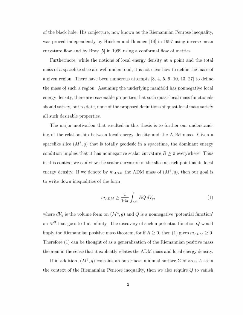
of the black hole. His conjecture, now known as the Riemannian Penrose inequality,

was proved independently by Huisken and Ilmanen [14] in 1997 using inverse mean

curvature flow and by Bray [5] in 1999 using a conformal flow of metrics.

Furthermore, while the notions of local energy density at a point and the total

mass of a spacelike slice are well understood, it is not clear how to define the mass of

a given region. There have been numerous attempts [3, 4, 5, 9, 10, 13, 27] to define

the mass of such a region. Assuming the underlying manifold has nonnegative local

energy density, there are reasonable properties that such quasi-local mass functionals

should satisfy, but to date, none of the proposed definitions of quasi-local mass satisfy

all such desirable properties.

The major motivation that resulted in this thesis is to further our understand-

ing of the relationship between local energy density and the ADM mass. Given a

spacelike slice (M3, g) that is totally geodesic in a spacetime, the dominant energy

condition implies that it has nonnegative scalar curvature R ≥ 0 everywhere. Thus

in this context we can view the scalar curvature of the slice at each point as its local

energy density. If we denote by mADM the ADM mass of (M3, g), then our goal is

to write down inequalities of the form

mADM ≥1

16π

∫M3

RQdVg, (1)

where dVg is the volume form on (M3, g) and Q is a nonnegative ‘potential function’

on M3 that goes to 1 at infinity. The discovery of such a potential function Q would

imply the Riemannian positive mass theorem, for if R ≥ 0, then (1) gives mADM ≥ 0.

Therefore (1) can be thought of as a generalization of the Riemannian positive mass

theorem in the sense that it explicitly relates the ADM mass and local energy density.

If in addition, (M3, g) contains an outermost minimal surface Σ of area A as in

the context of the Riemannian Penrose inequality, then we also require Q to vanish

2

along Σ and the ADM mass of (M3, g) to satisfy

mADM ≥√

A

16π+

1

16π

∫M3

RQdVg. (2)

While finding inequalities of the form (1) and (2) for an arbitrary complete, asymp-

totically flat manifold seems like a daunting task, we have succeeded in doing so for

manifolds that are graphs of smooth functions over Euclidean spaces. Moreover, our

argument is independent of the dimension of the manifold. Thus our result is valid

for all dimensions n ≥ 3.

In the process of our investigation, we have also discovered a new quasi-local

mass functional. Suppose Σ ⊂ M3 is a closed surface with Gauss curvature K > 0

and mean curvature H > 0, then the Weyl embedding theorem [17] implies that it

can be isometrically embedded into R3. Moreover, the embedding is unique up to

an isometry of R3. If H0 is the mean curvature of Σ under such embedding, then we

define the quasi-local mass of Σ to be

mQL(Σ) =1

16π

∫Σ

1

H0

(H20 −H2)dA.

and show that this definition has several useful properties.

In Chapter 1, we start with a brief overview of spacetimes and state the definitions

of asymptotic flatness and the ADM mass. At this point, various examples of asymp-

totically flat manifolds are introduced. In particular, we study the 3-dimensional

Schwarzschild manifold, which plays an important role in subsequent chapters. We

conclude this chapter with discussions of the Riemannian positive mass theorem and

the Riemannian Penrose inequality, which are two of the most important results

regarding the ADM mass.

Chapter 2 gives a brief overview of the inverse mean curvature flow proof of

the Riemannian Penrose inequality. In the process, the Hawking mass, which is an

3

example of a quasi-local mass functional, is introduced. The main purpose of this

chapter is to motivate inequalities of the form (1) and (2).

Chapter 3 starts by discussing the fact that a 3-dimensional Schwarzschild mani-

fold can be isometrically embedded as a rotating parabola in R4, and that its exterior

region can be expressed as the graph of a smooth function. More generally, we study

properties of Riemannian manifolds that are graphs of smooth functions over Eu-

clidean space and derive the formula for their scalar curvatures in local coordinates.

We conclude the chapter by translating the notions of asymptotic flatness and the

ADM mass for such manifolds.

We state and prove the first major result of this thesis in Chapter 4, namely, that

the ADM mass of a complete, asymptotically graph over Rn can be expressed as an

integral of the product of the scalar curvature and a nonnegative potential function.

The key lemma we need is that the scalar curvature of a graph is precisely the

divergence of a certain vector field. We also show in this chapter the surprising fact

that the ADM mass of a spherically symmetric graph over Rn must be nonnegative,

even without the nonnegative scalar curvature assumption. Finally, we express the

ADM mass of a graph over any asymptotically flat manifold as an integral involving

the scalar curvature of the base manifold.

We proceed to study graphs in the context of the Penrose inequality in Chapter

5. If a graph has a smooth minimal boundary whose connected components are

in level sets of the graph function f , then we express the ADM mass of the graph

as the sum of an interior integral over the manifold and a surface integral along

the minimal boundary. Furthermore, with the additional assumption that each con-

nected component of the boundary is convex, we prove the Penrose inequality via

the Aleksandrov-Fenchel inequality. We also point out that most of the contents of

Chapter 4 and 5 appear in [16].

In Chapter 6, we will apply the methods of Chapter 4 and Chapter 5 to study

4

graphs in Minkowski space. It turns out Minkowski space is the natural setting in

which zero area singularities (ZAS) arise. We begin this chapter by discussing the

notion of ZAS, following [6]. Our goal in this chapter is to prove the ZAS inequality

[6] for graphs in Minkowski space.

Finally in Chapter 7, we study in details the quasi-local mass functional that

arises in Chapter 5. If (Mn, g) is the graph of an asymptotically flat smooth function

over Rn with nonnegative scalar curvature, we show that our definition of quasi-

local mass is nonnegative, monotonically nondecreasing and asymptotic to mADM(g).

Moreover, our definition is also valid for a closed surface in a general asymptotically

flat 3-manifold (M3, g) whenever the Brown-York mass is defined. We also show that

a result of Shi and Tam [26] implies that our definition is nonnegative in this setting.

5

1

Technical Background

1.1 Spacetimes and Einstein’s equation

A spacetime [18] (N4, g) is a connected, time-oriented 4-dimensional Lorentzian man-

ifold of signature (−,+,+,+). A tangent vector v on N4 is called

1. timelike if g(v, v) < 0,

2. null (or light-like) if g(v, v) = 0, or

3. spacelike if g(v, v) > 0.

A vector field X on a Lorentzian manifold (N4, g) is timelike (resp. null or spacelike)

if at every point p ∈ N4, g(Xp, Xp) < 0 (resp. g(Xp, Xp) = 0 or g(Xp, Xp) > 0). If

(N4, g) admits a smooth, timelike vector field X, then it is said to be time-orientable

and the manifold with such a choice of X is called time-oriented. Note that these

terminologies arise from the fact that X distinguishes timelike or null vectors v as

future-pointing if g(X, v) < 0 or past-pointing if g(X, v) > 0.

6

Let Ric denote the Ricci curvature tensor and R the scalar curvature of g. We

assume that (N4, g) satisfies Einstein’s equation,

Ric− 1

2R · g = 8πT,

where T is called the stress-energy tensor of the spacetime. If T vanishes identically,

then we say that the spacetime is vacuum. A reasonable assumption on (N4, g) is

for it to have nonnegative energy density everywhere. This condition is called the

dominant energy condition and it stipulates that

T (v, w) ≥ 0

for all future timelike vectors v and w.

Furthermore, we assume that (N4, g) possesses a smooth 3-dimensional subman-

ifold M3 (i.e., a hypersurface) that is spacelike, which means every tangent vector of

M3 is spacelike when viewed as a vector in N4. This implies that the restriction of

g to M3 is a Riemannian metric g on M3. Such a hypersurface is called a spacelike

slice of the spacetime.

Given a spacelike slice (M3, g) of the spacetime, the stress-energy tensor gives

the notions of local energy density and local current density at a point in the slice.

Suppose n is a future-pointing unit normal vector to (M3, g), then we define the

local energy density to be µ = T (n, n) and the local current density to be the 1-form

J = T (n, ·). Thus Einstein’s equation gives

µ =1

16π(R− (trgh)2 + ‖h‖2

g)

J =1

8π∇g · (h− (trgh) · g),

(1.1)

where R is the scalar curvature of (M3, g), h is the second fundamental form of

(M3, g) in (N4, g), ‖ · ‖g is the norm with respect to g, and we use ∇g· to denote the

7

divergence operator on (M3, g). Moreover, the dominant energy condition implies

that

µ ≥ ‖J‖g.

Now if we restrict our attention to spacelike slices (M3, g) whose second funda-

mental form h in the spacetime is identically zero, then equation (1.1) becomes

µ =R

16πand J = 0.

In other words, the local energy density is proportional to the scalar curvature of g.

In this case, the dominant energy condition implies

R ≥ 0.

For the rest of this thesis, we will no longer discuss spacetimes. In fact, since the

dominant energy condition on (M3, g) consists solely of the scalar curvature of g, we

can generalize our discussions to manifolds (Mn, g) of any dimensions n ≥ 3.

1.2 Asymptotic flatness and the ADM mass

The main object of study in this thesis is the total mass (called the ADM mass) of

an asymptotically flat manifold. Roughly speaking, an n-dimensional Riemannian

manifold (Mn, g) is asymptotically flat if outside a compact subset K, Mn is dif-

feomorphic to the complement of the closed ball B1 = |x| ≤ 1 in Rn, and that

the metric g decays sufficiently fast to the flat Euclidean metric at infinity. More

precisely,

Definition 1. [21] A Riemannian manifold (Mn, g) of dimension n is said to be

asymptotically flat if it satisfies the following two conditions:

1. there exists a compact subset K ⊂ Mn and a diffeomorphism Φ : E =

Mn\K → Rn\B1,

8

2. in the coordinate chart (x1, x2, . . . , xn) on E defined by Φ,

g = gij(x)dxidxj,

where

gij(x) = δij +O(|x|−p)

|x||gij,k(x)|+ |x|2|gij,kl(x)| = O(|x|−p)

|R(x)| = O(|x|−q)

(1.2)

for all i, j, k, l = 1, 2, . . . , n, where gij,k = ∂kgij and gij,kl = ∂k∂lgij are the

coordinate derivatives of the ij-component of the metric, q > n and p > (n−

2)/2 are constants and R(x) is the scalar curvature of g at a point x.

The set E is called the end of the asymptotically flat manifold. More generally,

we say that (Mn, g) is an asymptotically flat manifold with multiple ends if Mn\K

is the disjoint union of ends Ek such that each end Ek is diffeomorphic to Rn\B1,

and that the metric in each end satisfies the decay condition (1.2). See for example

p.238 - 239 of [5] for the precise definition of an asymptotically flat manifold with

multiple ends. For our purpose, an asymptotically flat manifold always has one end

unless specified otherwise. In addition, we will make the extra assumption that an

asymptotically flat manifold is always connected. We also point out that Bartnik

explored the threshold values of 12

and 3 for p and q in [2].

For an asymptotically flat manifold (Mn, g), we can define its ADM mass:

Definition 2. [21] The ADM mass mADM(Mn, g) of an asymptotically flat mani-

fold (Mn, g) is defined to be

mADM(Mn, g) = limr→∞

1

2(n− 1)ωn−1

∫Sr

n∑i,j=1

(gij,i − gii,j)νjdSr,

9

where ωn−1 is the volume of the n − 1 unit sphere, Sr is the coordinate sphere of

radius r, ν is the outward unit normal to Sr and dSr is the area element of Sr in the

coordinate chart.

The physicists Arnowitt, Deser and Misner [1] first proposed this definition in

dimension n = 3 to describe the total mass in an isolated gravitational system.

We generalize their definition of the ADM mass to any dimension n ≥ 3 by choos-

ing the correct constant in front of the integral. We also point out that in [2],

Bartnik showed that the ADM mass is independent of the choice of asymptot-

ically flat coordinates. We will often omit the argument Mn (or g) and write

mADM(Mn, g) = mADM(g) = mADM if the manifold or the metric is understood.

Moreover, we will use the convention that repeated indices are automatically being

summed over. Thus we will henceforth write

mADM = limr→∞

1

2(n− 1)ωn−1

∫Sr

(gij,i − gii,j)νjdSr.

1.3 Examples of asymptotically flat manifolds

1. The simplest example of a complete asymptotically flat manifold is the Eu-

clidean space Rn with the standard flat metric g = δ. Since δij,k=0 for all i, j

and k, its ADM mass is 0. We will see later that this is in fact the rigidity case

of the Riemannian positive mass theorem.

2. If (Mn, g) is an asymptotically flat manifold, then one can easily construct a

class of asymptotically flat manifolds using a conformal change of metrics. We

say that a metric g is conformal to g if

g = u(x)4

n−2 g

for some u(x) ∈ C∞(Mn). Because of the exponent 4n−2

, we can without loss

of generality assume u(x) ≥ 0. Note that the choice of the exponent is a

10

convenient one since it simplifies the transformation of the scalar curvature: If

R and R are the scalar curvatures of g and g respectively, then

R = u(x)−(n+2n−2

)

(−4(n− 1)

(n− 2)∆gu+Ru.

)(1.3)

If (Mn, g) is asymptotically flat, then (Mn, g) is also an asymptotically flat

manifold given that u(x) satisfies suitable decay conditions. In particular,

(Mn, g) is asymptotically flat if

u→ 1 at ∞

ui = O(|x|−p−1)

ujk = O(|x|−p−2)

∆gu = O(|x|−q)

for some constants p > 12

and q > 3.

It is an easy calculation to show that the ADM masses of g and g and related

by

mADM(g) = mADM(g)− limr→∞

2

(n− 2)ωn−1

∫Sr

∂u

∂νdSr, (1.4)

where ∂u∂ν

is the outward normal derivative of u along Sr.

3. As a special case of example 2, let (M3, g) = (R3\0, u4δ) with u = 1 + m2r

,

where m is a positive constant and r =√x2 + y2 + z2 is the Euclidean distance

from the origin. Then the resulting manifold,

(M3, g) =

(R3\0,

(1 +

m

2r

)4

δ

),

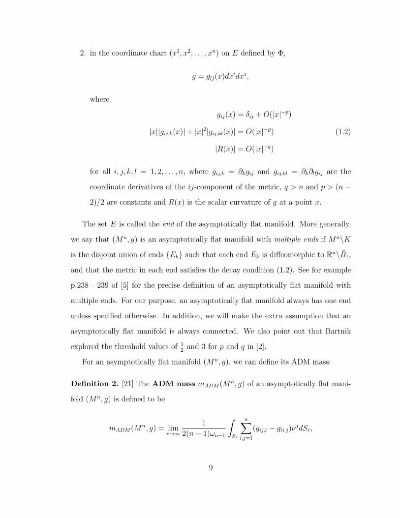
is a complete asymptotically flat manifold. This is called the 3-dimensional

Schwarzschild manifold. As we will show in Chapter 3, it can be isometrically

11

Σ = Sm/2

x→∞

x→ 0

(R3\0, (1 + m2r

)4δ)

Figure 1.1: Visualization of the 3-dimensional Schwarzschild manifold.

embedded as a rotating parabola in R4. Hence we can visualize it in as in

Figure 1.1.

Since R = 0 for the flat Euclidean metric and ∆u = 0, (1.3) implies that

the Schwarzschild manifold is scalar flat. Moreover, the hypersurface Sm/2 =

|x| = m/2 is a minimal surface in (M3, g), for if g = u(x)4δ, then the mean

curvature H of a sphere with respect to g satisfies

H =1

u2

(2

r+

4

u

∂u

∂r

), (1.5)

and H = 0 if r = m/2.

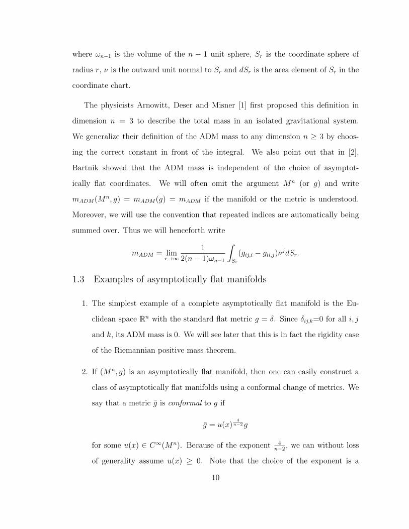
Furthermore, the 3-dimensional Schwarzschild manifold has two ends, with a

reflection symmetry about the minimal sphere Σ = Sm/2. We will from now on

refer to the outer end, given by

(R3\Bm/2,

(1 +

m

2r

)4

δ

),

12

as the exterior Schwarzschild manifold. This is now a complete asymptotically

flat manifold with one end that has a minimal boundary.

Σ = Sm/2

x→∞(R3\Bm/2, (1 + m

2r)4δ)

Figure 1.2: The exterior 3-dimensional Schwarzschild manifold.

Using (1.4), we can compute the ADM mass of the exterior Schwarzschild

manifold (M3, g) = (R3\Bm/2, (1 + m2r

)4δ):

mADM(g) = mADM(δ)− limr→∞

1

2π

∫Sr

∂

∂r

(1 +

m

2r

)4

dSr

= − limr→∞

1

2π

∫Sr

4(

1 +m

2r

)3 (− m

2r3

)dSr

= − limr→∞

1

2π· 4πr2 · 4

(1 +

m

2r

)3 (− m

2r3

)= m.

Thus the ADM mass of the exterior Schwarzschild manifold is precisely the

positive constant m.

1.4 Fundamental theorems on the ADM mass

Let us again focus on dimension n = 3 for the moment. Since the local energy

density of (M3, g) is µ = R16π

, one would expect the total mass of (M3, g) to equal

the integral of the local energy density over the manifold, that is,

mADM =1

16π

∫M3

RdVg.

13

But unfortunately this is not true in general as we can see from the last example.

For the 3-dimensional exterior Schwarzschild manifold,

mADM = m > 0 =1

16π

∫M3

RdVg

since R = 0 at every point. On the other hand, if we assume the dominant energy

condition is satisfied, then nonnegative scalar curvature everywhere should tell us

something about the ADM mass of the manifold. There are indeed two fundamental

theorems relating nonnegative scalar curvature and the ADM mass. The first result

is the following:

Theorem 3 (Riemannian Positive Mass Theorem). If (M3, g) is a complete,

asymptotically flat Riemannian 3-manifold with nonnegative scalar curvature and

ADM mass mADM , then

mADM ≥ 0,

with mADM = 0 if and only if (M3, g) is isometric to R3 with the standard flat metric.

Note that the adjective ‘Riemannian’ denotes the case in which the hypersurface

in the spacetime has zero second fundamental form, since in this case the statement

is purely one in Riemannian geometry about complete asymptotically manifolds with

nonnegative scalar curvature. In 1979, Schoen and Yau [22] gave a proof of Theo-

rem 3 using minimal surface techniques and a stability argument. In a follow-up

paper shortly after [23], they showed that their argument is valid for all dimensions

n ≤ 7. In 1981, Witten [28] gave an alternate proof of the positive mass theorem

using spinors and the Dirac operator in all dimensions with the assumption that the

manifold is spin.

Once again considering the 3-dimensional exterior Schwarzschild metric, we see

that the local energy density does not give any contribution to the mass. This

14

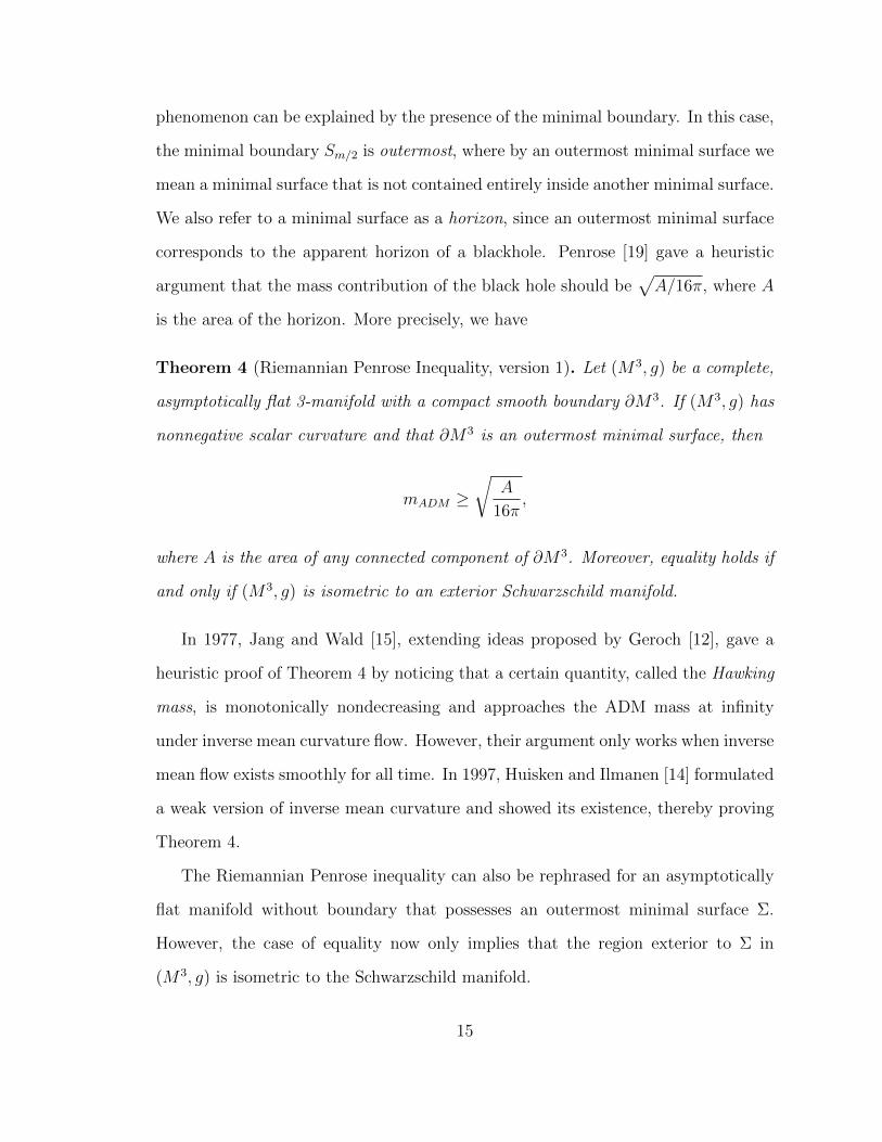
phenomenon can be explained by the presence of the minimal boundary. In this case,

the minimal boundary Sm/2 is outermost, where by an outermost minimal surface we

mean a minimal surface that is not contained entirely inside another minimal surface.

We also refer to a minimal surface as a horizon, since an outermost minimal surface

corresponds to the apparent horizon of a blackhole. Penrose [19] gave a heuristic

argument that the mass contribution of the black hole should be√A/16π, where A

is the area of the horizon. More precisely, we have

Theorem 4 (Riemannian Penrose Inequality, version 1). Let (M3, g) be a complete,

asymptotically flat 3-manifold with a compact smooth boundary ∂M3. If (M3, g) has

nonnegative scalar curvature and that ∂M3 is an outermost minimal surface, then

mADM ≥√

A

16π,

where A is the area of any connected component of ∂M3. Moreover, equality holds if

and only if (M3, g) is isometric to an exterior Schwarzschild manifold.

In 1977, Jang and Wald [15], extending ideas proposed by Geroch [12], gave a

heuristic proof of Theorem 4 by noticing that a certain quantity, called the Hawking

mass, is monotonically nondecreasing and approaches the ADM mass at infinity

under inverse mean curvature flow. However, their argument only works when inverse

mean flow exists smoothly for all time. In 1997, Huisken and Ilmanen [14] formulated

a weak version of inverse mean curvature and showed its existence, thereby proving

Theorem 4.

The Riemannian Penrose inequality can also be rephrased for an asymptotically

flat manifold without boundary that possesses an outermost minimal surface Σ.

However, the case of equality now only implies that the region exterior to Σ in

(M3, g) is isometric to the Schwarzschild manifold.

15

In 1999, Bray [5] proved the following more general version of Theorem 4 using a

different approach by defining a conformal flow of metrics. His proof generalizes in

two ways. First, A is now the total area of the horizon. Second, ‘outermost horizon’

is replaced by ‘outer minimizing horizon’. A horizon is (strictly) outer minimizing

if every other surface which encloses it has (strictly) greater area. This is a slight

generalization since outermost horizons are always strictly outer minimizing.

Theorem 5 (Riemannian Penrose Inequality, version 2). Let (M3, g) be a complete,

asymptotically flat 3-manifold with nonnegative scalar curvature and an outer mini-

mizing horizon of total area A. Then

mADM ≥√

A

16π,

with equality if and only if (M3, g) is isometric to a Schwarzschild manifold outside

their respective outer minimizing horizon.

In [8], Bray and Lee generalized Bray’s proof of Theorem 5 to dimension n ≤

7, with the extra assumption that the manifold is spin for the equality case. In

dimension n, the Riemannian Penrose inequality is

mADM ≥1

2

(A

ωn−1

)n−2n−1

.

We point out that the Riemannian Penrose inequality remains widely open for dimen-

sion 8 or higher except in the spherically symmetric case, though recently Schwartz

[25] proved a type of volumetric Penrose inequality for conformally flat manifolds in

all dimensions.

16

2

The Inverse Mean Curvature Flow and IntegralPenrose Inequality

In this chapter we give a brief overview of the inverse mean curvature flow proof of

Theorem 4. Our main goal is to motivate inequalities of the form

mADM ≥1

2(n− 1)ωn−1

∫Mn

RQdVg (2.1)

for a complete, asymptotically flat manifold (Mn, g) with ADM mass mADM , and

mADM ≥1

2

(A

ωn−1

)n−2n−1

+1

2(n− 1)ωn−1

∫Mn

RQdVg (2.2)

if (Mn, g) possesses an outermost minimal surface Σ and A = |Σ| is the (n − 1)

volume of Σ. Note that (2.1) and (2.2) are the n-dimensional versions of (1) and (2).

See [14, 5, 7] for more in-depth discussions of inverse mean curvature flow and the

Riemannian Penrose inequality.

17

2.1 Inverse mean curvature flow and the Hawking mass

Let Σ be a 2-dimensional closed surface in (M3, g). A foliation of Σ in M3 in the

normal direction with flow speed η is a smooth family F : Σ × [0, T ] → M of

hypersurfaces Σt := F (Σ, t) satisfying the evolution equation

∂F

∂t= ην, x ∈ Σt, 0 ≤ t ≤ T, (2.3)

where η is a smooth function on Σt, ν is the outward unit normal to Σt and ∂F∂t

is

the normal velocity vector field along the surface Σt. We also allow the possibility

that T = ∞. If we choose η = 1H

, where H is the mean curvature of Σt at a point

x ∈ Σt, then we obtain the inverse mean curvature flow:

∂F

∂t=

ν

H. (2.4)

Note that this is a parabolic evolution equation.

Now given a closed surface Σ in (M3, g), with area |Σ| with respect to the induced

metric from g and mean curvature H, its Hawking mass is defined to be

mH(Σ) =

√|Σ|16π

(1− 1

16π

∫Σ

H2dA

).

Suppose (M3, g) satisfies the hypotheses of Theorem 4. If Σ is a connected

component of the outermost horizon ∂M3 and that inverse mean curvature flow with

Σ as the initial surface exists smoothly for all time 0 ≤ t <∞, then mH satisfies the

following three properties:

1. If the initial surface Σ is minimal, then mH(Σ) =√|Σ|16π

. Note that this is the

lower bound for the ADM mass in the Riemannian Penrose inequality.

2. The Hawking mass is monotonically nondecreasing under inverse mean curva-

ture flow. Namely, if Σt is a family of hypersurfaces satisfying (2.4) with

18

Σ0 = Σ, then

d

dtmH(Σt) ≥ 0 for all t. (2.5)

(2.5) is known as the Geroch-Jang-Wald monotonicity formula.

3. The Hawking mass of sufficiently round spheres at infinity in the asymptotically

flat end of (M3, g) approaches mADM . Hence

limt→∞

mH(Σt) = mADM(g)

if inverse mean curvature flow beginning with Σ eventually flows to sufficiently

round spheres at infinity.

The above properties of mH implies that

mADM(g) = limt→∞

mH(Σt) ≥ mH(Σ0) =

√|Σ|16π

,

which is the conclusion of Theorem 4. However, as noted by Jang and Wald, this

argument only works when inverse mean curvature flow exists and is smooth, which

in general is not the case. The main contribution of Huisken and Illmanen was that

they defined a weak version of the inverse mean curvature via a level-set formulation

and showed that this flow still exists and (2.5) remains valid.

To motivate the inequalities (2.1) and (2.2), we derive the monotonicity formula

(2.5) in the next section.

2.2 Geroch-Jang-Wald monotonicity formula

To derive (2.5), we begin with the first and second variation formulas of area. Suppose

Σt is a 1-parameter family of surfaces in (M3, g) satisfying (2.3), then the first

variation formula of area is

d

dt|Σt| =

∫Σt

ηHdAt,

19

where dAt is the area form on Σt induced by g. In other words,

d

dtdAt = ηHdAt.

Since the mean curvature gives the first variation of area, the second variation formula

of area can be thought of as the derivative of H:

d

dtH = −∆Σtη −Ric(ν, ν)η − ‖h‖2η,

where ∆Σt is the Laplacian of (M3, g) restricted along Σt, Ric is the Ricci tensor

of (M3, g), ν is the outward unit normal to Σt and ‖h‖ is the norm of the second

fundamental form h of Σt in (M3, g). Since η = 1H

under inverse mean curvature

flow, the variation formulas become

d

dtdAt = dAt

d

dtH = −∆Σt

1

H−Ric(ν, ν)

1

H− ‖h‖2 1

H.

We can now start computing

d

dtmH(Σt) =

d

dt

(√|Σt|16π

)(1− 1

16π

∫Σt

H2dAt

)+

√|Σt|16π

d

dt

(1− 1

16π

∫Σt

H2dAt

)

=1

2

√|Σt|16π

(1− 1

16π

∫Σt

H2dAt

)+

√|Σt|16π

(− 1

16π

∫Σt

2HdH

dt+H2dAt

)

=

√|Σt|16π

[1

2− 1

16π

∫Σt

2H

(−∆Σt

1

H−Ric(ν, ν)− ‖h‖2 1

H

)+

3

2H2dAt

]

=

√|Σt|16π

[1

2+

1

16π

∫Σt

2H∆Σt

1

H+ 2Ric(ν, ν) + 2‖h‖2 − 3

2H2dAt

].

To show that the derivative of the Hawking mass is nonnegative, we note the

following facts:

20

• Integrating by parts,∫Σt

2H∆Σt

1

HdAt =

∫Σt

−〈∇ΣtH,∇Σt

1

H〉dAt =

∫Σt

2|∇ΣtH|2

H2dAt.

• The Gauss equation:

Ric(ν, ν) =1

2R−K +

1

2H2 − 1

2‖h‖2,

where R is the scalar curvature of (M3, g) and K is the Gauss curvature of Σt.

• If λ1 and λ2 are the principal curvatures of Σt, then

‖h‖2 − 1

2H2 =

1

2(λ1 − λ2)2,

since H = λ1 + λ2 and ‖h‖2 = λ21 + λ2

2 by definition.

Using the above three facts,

d

dtmH(Σt) =

√|Σt|16π

[1

2+

1

16π

∫Σt

2|∇ΣtH|2

H2+R− 2K +

1

2(λ1 − λ2)2

]

≥√|Σt|16π

(1

2− 1

8π

∫Σt

K dAt

)≥ 0

since ∫Σt

K ≤ 4π

by the Gauss-Bonnet Theorem.

2.3 Integral Penrose inequality and potential function Q

In fact, Bray and Khuri [7] noticed that the derivation of (2.5) reveals more. In

particular, we actually have

d

dtmH(Σt) ≥

√|Σt|16π· 1

16π

∫Σt

RdAt.

21

Now integrate this inequality in t from 0 to ∞,

∫ ∞0

d

dtmH(Σt)dt ≥

1

16π

∫ ∞0

∫Σt

R

√|Σt|16π

dAtdt. (2.6)

By the fundamental theorem of calculus, the left hand side of (2.6) is

limr→∞

mH(Σr)−mH(Σ0) = mADM(g)−√

A

16π

by the properties 1 and 3 of mH . To rewrite the right hand side of (2.6), we use the

co-area formula

dAtdt =1

ηdVg = HdVg.

Thus (2.6) becomes

mADM −√

A

16π≥ 1

16π

∫M3

R ·H√|Σt|16π

dVg

mADM ≥√

A

16π+

1

16π

∫M3

RQdVg,

(2.7)

for Q = H√|Σt|16π

. Notice that if inverse mean curvature flow exists smoothly for all

time and eventually flows to sufficiently round spheres, then Q ≥ 0 and Q → 1 at

infinity, and the above inequality is actually stronger statement than the Riemannian

Penrose inequality since R ≥ 0 implies

mADM ≥√

A

16π+

1

16π

∫M3

RQdVg ≥√

A

16π.

In light of inequality (2.7), one could attempt to prove the Riemannian Penrose

inequality by finding a nonnegative potential function Q such that

mADM ≥√

A

16π+

1

16π

∫M3

RQdVg.

22

Q = H√|Σt|16π

from inverse mean curvature flow is one such example, but if the

outermost horizon Σ is not connected, then A is only the area of one of the connected

components of Σ. Moreover, this only works in dimension n = 3 as the Geroch-Jang-

Wald monotonicity formula (2.5) relies critically on the Gauss-Bonnet Theorem.

More generally, given a complete, asymptotically flat manifold (Mn, g) (without

boundary) with R ≥ 0 and ADM mass mADM , we would like to find such a ‘potential

function Q’ such that

1. Q ≥ 0 on Mn,

2. Q→ 1 at ∞, and

3. mADM ≥1

2(n− 1)ωn−1

∫Mn

RQdVg.

If (Mn, g) has an outermost (or more generally, outer minimizing) boundary Σ =

∂Mn of area A, then Q should vanish on Σ and mADM should satisfy

mADM ≥1

2

(A

ωn−1

)n−2n−1

+1

2(n− 1)ωn−1

∫Mn

RQdVg.

23

3

Graphs over Euclidean Space

In this chapter, we study complete, asymptotically flat manifolds that are the graphs

of smooth functions over Rn. We begin by discussing the fact that the 3-dimensional

Schwarzschild manifold can be isometrically embedded into R4 as a rotating parabola,

and that its exterior region can be expressed as the graph of a smooth function.

We then proceed to study manifolds that are graphs of functions over Euclidean

space in general and derive the formula of the scalar curvature of such manifolds in

coordinates.

3.1 Motivation: Schwarzschild manifold as a graph

The equality cases of the Riemannian positive mass theorem and Penrose inequality

are the distinguished cases, and we would hope that they can further our under-

standing of the relationship between local energy density and the ADM mass. The

equality case of the Riemannian positive mass theorem is simply the flat Euclidean

space Rn, so that does not seem to give us much insights. On the other hand, the

Schwarzschild manifold, which is the equality case of the Riemannian Penrose in-

equality, appears to be more interesting. In dimension n = 3, the Schwarzschild

24

manifold is conformal to R3\0 and may be expressed as(R3\0,

(1 +

m

2r

)4

δ

),

where m is a positive constant, r =√x2 + y2 + z2 is the Euclidean distance of the

point (x, y, z) from the origin in R3 and δ is the flat Euclidean metric. Moreover, the

3-dimensional Schwarzschild manifold has another very interesting property, namely,

that it can be isometrically embedded as a rotating parabola in R4 as the set of

points (x, y, z, w) ⊂ R4 satisfying |(x, y, z)| = w2

8m+ 2m:

Figure 3.1: The three dimensional Schwarzschild metric of mass m > 0 (in blue)viewed as a spherically symmetric submanifold of four dimensional Euclidean space(x, y, z, w) satisfying R = w2/8m+2m, where R =

√x2 + y2 + z2. Figure courtesy

of Hubert Bray.

Explicitly, the inverse of the above isometric embedding is given by

φ : r =w2

8m+ 2m ⊂ R4 → R3\0

φ(r, w) =

((1 +

m

2r

)−2

r

)Notice that under the isometric embedding, the image of the minimal surface Sm/2 =

|x| = m/2 ⊂ R3\0 is S2m = (x, y, z, 0) :√x2 + y2 + z2 = 2m ⊂ R4, and the

exterior Schwarzschild manifold corresponds to the points such that w ≥ 0.

25

In particular, solving for w, we see that the exterior 3-dimensional Schwarzschild

metric is the graph of the spherically symmetric function f : R3\B2m(0)→ R given

by f(r) =√

8m(r − 2m). In this case, one can check directly that the ADM mass

of (M3, g) is the positive constant m by computing a certain boundary integral at

infinity involving the function f .

That an end of the three dimensional Schwarzschild metric can be isometrically

embedded in R4 as the graph of a function over R3\B2m raises the following questions:

if Ω is a bounded open set in Rn with smooth boundary Σ = ∂Ω, and f is a smooth

function on Rn\Ω such that the graph of f is an asymptotically flat manifold (Mn, g)

with the induced metric g from Rn+1, has nonnegative scalar curvature R ≥ 0 and

horizon f(Σ), can we prove the Penrose inequality for (Mn, g) using elementary

techniques in this setting? And if so, do can get a stronger statement than the

standard Penrose inequality? We answer both questions in the affirmative, and we

begin by proving a stronger version of the Riemannian positive mass theorem for

manifolds that are graphs over Rn in Chapter 4 by expressing R as a divergence

and applying the divergence theorem, giving the ADM mass as an integral over the

manifold of the product of R and a nonnegative potential function. In the presence

of a boundary whose connected components are convex, we prove a stronger Penrose

inequality by giving lower bounds to the boundary integrals using the Aleksandrov-

Fenchel inequality. Before proceeding further, we will present some basic properties

of asymptotically flat manifolds that are graphs over Rn.

3.2 Graphs over Euclidean space

If f : Rn → R is a smooth function, then the graph of f is a hypersurface in Rn+1.

Moreover,

26

Proposition 6. Let f : Rn → R be a smooth function and let

Mn = (x1, . . . , xn, f(x1, . . . , xn)) ∈ Rn+1 : (x1, . . . , xn) ∈ Rn

be the graph of f . If Mn is equipped with the metric g induced from the flat metric

on Rn+1, then (Mn, g) is isometric to (Rn, δ+ df ⊗ df), where δ is the flat metric on

Rn.

Proof. Let x = (x1, . . . , xn) be the standard coordinates on Rn and (x, xn+1) the

coordinates on Rn+1. We show that the map

F : (Rn, δ + df ⊗ df)→ (Mn, g)

x 7→ (x, f(x))

is an isometry. Since f is smooth by assumption, F is clearly a smooth map.

Moreover, F is a diffeomorphism whose smooth inverse is the projection map π :

(Mn, g)→ (Rn, δ + df ⊗ df) defined by π(x, f(x)) = x.

Next, we check that the diffeomorphism F is an isometry, namely, F ∗g = δ +

df ⊗ df . By the definition of the pullback F ∗,

(F ∗g)

(∂

∂xi,∂

∂xj

)= g

(F∗

∂

∂xi, F∗

∂

∂xj

)

for all i, j = 1, . . . , n. If φ ∈ C∞(Mn, g), then(F∗

∂

∂xi

)φ =

∂

∂xi(φ F ) =

∂

∂xi(φ(x, f(x)))

=

(n+1∑k=1

∂φ

∂xk∂xk

∂xi

)

=∂φ

∂xn+1

∂f

∂xi+

(n∑k=1

∂φ

∂xk∂xk

∂xi

)

=

(∂

∂xi+∂f

∂xi∂

∂xn+1

)φ.

27

Thus

F∗∂

∂xi=

∂

∂xi+ fi

∂

∂xn+1,

where we have used the shorthand notation fi = ∂f∂xi

to denote the i-coordinate

derivative of f . Since g is the induced metric from Rn+1, we have

g

(∂

∂xi,∂

∂xj

)= δij for 1 ≤ i, j ≤ n+ 1

and

g

(F∗

∂

∂xi, F∗

∂

∂xj

)= g

(∂

∂xi+ fi

∂

∂xn+1,∂

∂xj+ fj

∂

∂xn+1

)= δij + fifj.

Remark 7. Because of Proposition 6, we will from now on refer to

(Mn, g) = (Rn, δ + df ⊗ df)

as the graph of the function f . More generally, if Ω ⊂ Rn is a bounded open set with

smooth boundary Σ = ∂Ω, then the graph of a smooth function f equipped with the

induced metric g is a complete manifold with boundary f(Σ), and it is isometric to

(Rn\Ω, δ + df ⊗ df). We study such manifolds in Chapter 5

Since our goal is to understand the relationship between the ADM mass and the

scalar curvature of a graph manifold, our next task is to compute the scalar curvature

of a graph. Since we have a natural choice of global coordinates on the graph from

the proof of the previous proposition, we will do our calculations in this coordinate

chart.

Let (Mn, g) = (Rn, δ + df ⊗ df) be the graph of a smooth function f : Rn → R.

Since gij = δij + fifj, the inverse of gij is

gij = δij − f if j

1 + |∇f |2,

28

Rn

R

(Mn, g) ∼= (Rn, δ + df ⊗ df)

f

Figure 3.2: The graph of a smooth function f over Rn

where the norm of ∇f is taken with respect to the flat metric δ on Rn. We verify

this with the following calculation:

gijgjk = (δij + fifj)

(δjk − f jfk

1 + |∇f |2

)

= δijδjk + fifjδ

jk − δijf jfk

1 + |∇f |2− fifjf

jfk

1 + |∇f |2

= δki + fifk − fif

k(1 + |∇f |2)

1 + |∇f |2

= δki .

Using the fact gij,k = ∂k(δij + fifj) = fikfj + fifjk, we compute the Christoffel

29

symbols Γkij of (Mn, g):

Γkij =1

2gkm(gim,j + gjm,i − gij,m)

=1

2

(δkm − fkfm

1 + |∇f |2

)(fijfm + fifjm + fijfm + fjfim − fimfj − fifjm)

=1

2

(δkm − fkfm

1 + |∇f |2

)2fijfm

= fijfk − fijf

k|∇f |2

1 + |∇f |2

=fijf

k

1 + |∇f |2.

Remark 8. Since the indices are raised and lowered using the flat metric on Rn, it will

be notationally more convenient from now on to write everything as lower indices,

with the implicit assumption that any repeated indices are being summed over as

usual.

With the above remark in mind, we have

Γkij =fijfk

1 + |∇f |2

Γkij,k =fijkfk

1 + |∇f |2+

fijfkk1 + |∇f |2

− 2fijfklfkfl(1 + |∇f |2)2

.

The scalar curvature R in local coordinates is [21]

R = gij(Γkij,k − Γkik,j + ΓlijΓkkl − ΓlikΓ

kjl).

30

For a graph, the terms involving the Christoffel symbols are

Γkij,k =fijkfk

1 + |∇f |2+

fijfkk1 + |∇f |2

− 2fijfklfkfl(1 + |∇f |2)2

Γkik,j =fijkfk

1 + |∇f |2+

fikfjk1 + |∇f |2

− 2fikfjlfkfl(1 + |∇f |2)2

ΓlijΓkkl =

fijfklfkfl(1 + |∇f |2)2

ΓlikΓkjl =

fikfjlfkfl(1 + |∇f |2)2

We now proceed to derive the formula of the scalar curvature of a graph:

R = gij(Γkij,k − Γkik,j + ΓlijΓkkl − ΓlikΓ

kjl)

=

(δij −

fifj1 + |∇f |2

)(fijkfk

1 + |∇f |2+

fijfkk1 + |∇f |2

− 2fijfklfkfl(1 + |∇f |2)2

− fijkfk1 + |∇f |2

− fikfjk1 + |∇f |2

+2fikfjlfkfl

(1 + |∇f |2)2+

fijfklfkfl(1 + |∇f |2)2

− fikfjlfkfl(1 + |∇f |2)2

)

=

(δij −

fifj1 + |∇f |2

)(fijfkk

1 + |∇f |2− fikfjk

1 + |∇f |2− fijfklfkfl

(1 + |∇f |2)2+

fikfjlfkfl(1 + |∇f |2)2

)

=1

1 + |∇f |2(fiifkk − fikfik)−

fkfl(1 + |∇f |2)2

(fiifkl − fikfil)

− fifj(1 + |∇f |2)2

(fijfkk − fikfjk)−fifjfkfl

(1 + |∇f |2)3(fijfkl − fikfjl)

=1

1 + |∇f |2(fiifkk − fikfik)−

fkfl(1 + |∇f |2)2

(fiifkl − fikfil)

− fifj(1 + |∇f |2)2

(fijfkk − fikfjk)

since

fifjfkfl(1 + |∇f |2)3

(fijfkl − fikfjl)

by symmetry when we sum over i, j, k and l. If we relabel the indices by sending k

31

to j in the first term, l to j in the second term and switching i and k in the third

term, we have

Proposition 9. The scalar curvature R of a graph (Rn, δ + df ⊗ df) is given by

R =1

1 + |∇f |2

(fiifjj − fijfij −

2fjfk1 + |∇f |2

(fiifjk − fijfik)). (3.1)

Alternately, we can also rewrite (3.1) using coordinate-free notations. Let ∆f

denote the Laplacian of f with respect to the flat metric and Hf the Hessian of f .

Then

fiifjj = (∆f)2

fijfij = ‖Hf‖2

fiifjkfjfk = (∆f)Hf (∇f,∇f)

fijfikfjfk = ‖Hf (∇f, ·)‖2,

where by Hf (∇f, ·) we mean the 1-form that takes a vector v to Hf (∇, v). Thus the

scalar curvature of a graph has the coordinate-free expression

R =1

1 + |∇f |2

((∆f)2 − ‖Hf‖2 − 2∆fHf (∇f,∇f) + 2‖Hf (∇f, ·)‖2

1 + |∇f |2

). (3.2)

3.3 Asymptotically flat graphs and ADM mass

The calculations in the previous section is valid for graphs over Rn, including ones

that are not asymptotically flat. Our next step is to translate the notion of asymp-

totic flatness and the ADM mass to graphs.

Definition 10. Let f : Rn → R be a smooth function and let fi denote the ith

partial derivative of f . We say that f is asymptotically flat if

fi(x) = O(|x|−p/2)

|x||fij(x)|+ |x|2|fijk(x)| = O(|x|−p/2)

32

at infinity for some p > (n− 2)/2.

Since gij = δij + fifj, gij,k = fikfj + fifjk for all i, j, k and

gij,i − gii,j = fiifj + fifij − fijfi − fifij = fiifj − fijfi.

Thus we can express the ADM mass of a graph in terms of f :

Definition 11. The ADM mass of a complete, asymptotically flat graph is defined

to be

mADM = limr→∞

1

2(n− 1)ωn−1

∫Sr

(fiifj − fijfi)νjdSr, (3.3)

where ωn−1 is the volume of the n − 1 unit sphere, Sr is the coordinate sphere of

radius r, ν is the outward unit normal to Sr and dSr is the area element of Sr in the

coordinate chart.

33

4

The Positive Mass Theorem for Graphs

In this chapter we derive an expression for the ADM mass of the graph (Mn, g) of

a smooth asymptotically flat function f : Rn → R involving the scalar curvature of

(Mn, g). More precisely, we prove

Theorem 12 (Positive mass theorem for graphs over Rn). Let (Mn, g) be the graph

of a smooth asymptotically flat function f : Rn → R with the induced metric from

Rn+1. Let R be the scalar curvature and mADM the ADM mass of (Mn, g). Let ∇f

denote the gradient of f in the flat metric and |∇f | its norm with respect to the flat

metric. Let dVg denote the volume form on (Mn, g). Then

mADM =1

2(n− 1)ωn−1

∫Mn

R1√

1 + |∇f |2dVg.

In particular, R ≥ 0 implies m ≥ 0.

Remark 13. Note that Theorem 12 gives an expression for the ADM mass regardless

of the sign of the scalar curvature. Thus Theorem 12 also holds for graphs that have

negative scalar curvature somewhere. On the other hand, we will see that Theorem

34

15 implies the scalar curvature of a graph in Rn+1 cannot be too negative in a certain

sense.

4.1 A naive approach via integration by parts

For motivation, we once again consider the 3-dimensional Schwarzschild manifold.

As we noted in Chapter 3, it can be isometrically embedded into R4 as a rotating

parabola, and that its exterior region outside the horizon may be expressed as the

graph of the spherically symmetric function f(x, y, z) =√

8m(r−2m)1/2 on R3\B2m,

where r =√x2 + y2 + z2. Recall also that Σ = S2m is the minimal boundary of the

Schwarzschild manifold when isometrically embedded in R4. Moreover, we have

expressed the ADM mass in terms of the graph function f in (3.3). Since the ADM

mass is defined as a boundary integral of the dot product of the vector field

(fiifj − fijfi)∂j

with the outward unit normal at ∞ , and that our goal is to bound the ADM mass

from below with an interior integral over the manifold and a surface integral along the

minimal boundary , the most obvious thing to try is to use the divergence theorem

and hope for the best. Since |∇f(x)| → ∞ as x → Σ, we cannot quite apply the

divergence theorem to R3\B2m directly. Instead, we apply the divergence theorem

to R3\B2m+ε for some ε > 0, hoping that the limit exists as ε → 0. Denote by dVδ

35

the flat Euclidean volume form, then we have

mADM = limr→∞

1

16π

∫Sr

(fiifj − fijfi)νjdSr

=1

16π

∫R3\B2m+ε

∇ · [(fiifj − fijfi)∂j]dVδ −1

16π

∫S2m+ε

(fiifj − fijfi)νjdA

=1

16π

∫R3\B2m+ε

fiijfj + fiifjj − fijjfi − fijfijdVδ

− 1

16π

∫S2m+ε

(fiifj − fijfi)νjdA

=1

16π

∫R3\B2m+ε

fiifjj − fijfijdVδ −1

16π

∫S2m+ε

(fiifj − fijfi)νjdA

because fiijfj = fijjfi by switching i and j.

If this method were to work, we would hope that as ε → 0, the second integral

in the last equation gives the mass of the minimal boundary. Because of this, let us

naively define the mass of the minimal boundary Σ = S2m as

mN(Σ) := limε→0

1

16π

∫S2m+ε

(fiifj − fijfi)νjdA. (4.1)

Suppose f = f(r) is a spherically symmetric function on R3 and let fr = ∂f/∂r

denote its radial derivative. By the chain rule, the coordinate derivatives of f satisfy

fi = frxir

fij = frrxixjr2

+ fr

(δijr− xixj

r3

).

Since the outward normal is νj = xj/r, we have

fiifjνj =

[frr

x2i

r2+ fr

(1

r− x2

i

r3

)]frxjr

xj

r

= frrfrx2ix

2j

r4+ f 2

r

(x2j

r3−x2ix

2j

r5

)

= frrfr +2f 2

r

r

(4.2)

36

and

fijfiνj =

[frr

xixjr2

+ fr

(δijr− xixj

r3

)]frxir

xj

r

= frrfrx2ix

2j

r4+ f 2

r

(δijxixjr3

−x2ix

2j

r5

)= frrfr.

(4.3)

Plugging (4.2) and (4.3) into (4.1) gives

mN(Σ) = limε→0

1

16π

∫S2m+ε

2

rf 2r dA.

For the Schwarzschild manifold, f =√

8m(r − 2m)1/2 and fr =√

2mr−2m

, thus

mN(Σ) = limε→0

1

16π

∫S2m+ε

2

r· 2m

r − 2mdA

= limε→0

1

16π· 4πr2 · 4m

r(r − 2m)

∣∣∣∣r=2m+ε

= limε→0

rm

r − 2m

∣∣∣∣r=2m+ε

= limε→0

(2m+ ε)m

ε

=∞,

which is bad, since we know the mass of the minimal boundary of the Schwarzschild

manifold should be m =√

A16π

.

On the other hand, we can try to amend the situation with the following obser-

vation: since the ADM is a boundary integral at ∞, we can multiply the integrand

in (3.3) by a function φ that goes to 1 at∞ without changing the ADM mass. Thus

mADM = limr→∞

1

16π

∫Sr

φ · (fiifj − fijfi)νjdSr.

37

If we start with this alternate definition of the ADM mass for the Schwarzschild

manifold, then the divergence theorem implies that the surface integral along the

minimal boundary is now

limε→0

1

16π

∫S2m+ε

φ · 4m

r(r − 2m)dA.

Having in mind that the mass of the horizon should be the number m, we can choose

φ = (r − 2m)/r to get the correct mass, since

limε→0

1

16π

∫S2m+ε

r − 2m

r· 4m

r(r − 2m)dA = m.

Moreover, the factor φ = (r − 2m)/r happens to be precisely 1/(1 + |∇f |2) for the

Schwarzschild manifold:

1

1 + |∇f |2=

1

1 + f 2r

=

(1 +

2m

r − 2m

)−1

=r − 2m

r.

Therefore if we choose φ = 1/(1 + |∇f |2) and write the ADM mass of a graph as

mADM = limr→∞

1

16π

∫Sr

1

1 + |∇f |2(fiifj − fijfi)νjdA, (4.4)

the divergence theorem may allow us to prove the positive mass theorem for graphs.

In fact, this will work perfectly because of a key lemma in the next section.

4.2 The positive mass theorem

Equation (4.4) says that the ADM mass of a graph is a boundary integral at ∞ of

the vector field

1

1 + |∇f |2(fiifj − fijfi)∂j. (4.5)

Once again having in mind the divergence theorem, we would hope that the diver-

gence of (4.5) is an expression involving the scalar curvature of the graph. Just as

luck will have it, it turns out this divergence is precisely the scalar curvature.

38

Lemma 14. The scalar curvature R of the graph (Rn, δ + df ⊗ df) satisfies

R = ∇ ·(

1

1 + |∇f |2(fiifj − fijfi)∂j

).

Proof. Since we know what to look for, this is just a direct calculation:

∇ ·(

1

1 + |∇f |2(fiifj − fijfi)∂j

)

=1

1 + |∇f |2(fiijfj + fiifjj − fijjfi − fijfij)−

2fjkfk(1 + |∇f |2)2

(fiifj − fijfi)

=1

1 + |∇f |2

(fiifjj − fijfij −

2fjfk1 + |∇f |2

(fiifjk − fijfik))

= R

by Proposition 3.1.

We are now in the position to prove Theorem 12:

Proof of Theorem 12. By definition, the ADM mass of (Mn, g) = (Rn, δ+df ⊗df) is

mADM = limr→∞

1

2(n− 1)ωn−1

∫Sr

(gij,i − gii,j)νjdSr

= limr→∞

1

2(n− 1)ωn−1

∫Sr

(fiifj + fijfi − 2fijfi)νjdSr

= limr→∞

1

2(n− 1)ωn−1

∫Sr

(fiifj − fijfi)νjdSr.

By the asymptotic flatness assumption, the function 1/(1+|∇f |2) goes to 1 at infinity.

Hence we can alternately write the mass as

mADM = limr→∞

1

2(n− 1)ωn−1

∫Sr

1

1 + |∇f |2(fiifj − fijfi)νjdSr.

39

Now apply the divergence theorem in (Rn, δ) and use Lemma 14 to get

mADM =1

2(n− 1)ωn−1

∫Rn∇ ·(

1

1 + |∇f |2(fiifj − fijfi)∂j

)dVδ

=1

2(n− 1)ωn−1

∫RnRdVδ

=1

2(n− 1)ωn−1

∫Mn

R1√

1 + |∇f |2dVg

since

dVg =√

det gdVδ =√

1 + |∇f |2dVδ.

We also point out that we have not been able to prove the rigidity case of

the positive mass theorem, which says that assuming nonnegative scalar curvature,

mADM(Mn, g) = 0 implies that (Mn, g) is isometric to (Rn, δ). If mADM = 0, then

Theorem 12 gives

mADM =1

2(n− 1)ωn−1

∫Mn

R1√

1 + |∇f |2dVg = 0.

Assuming R ≥ 0, then 1/√

1 + |∇f |2 ≥ 0 implies that R ≡ 0. In other words, the

rigidity case of the positive mass theorem for graphs comes down to showing that if

a complete, asymptotically flat graph defined on all of Rn has R ≡ 0, then the graph

must be flat. Note the similarity of this statement with the Bernstein’s theorem,

which stipulates that if f is a smooth function on Rn such that the graph of f is a

minimal surface in Rn+1, then f must be a linear function. So

∇ ·(

∇f1 + |∇f |2

)= 0, f complete⇒ f is linear,

while to prove the rigidity case of the positive mass theorem for graphs, we need to

40

show

∇ ·(fiifj − fijfi1 + |∇f |2

∂j

)= 0, f complete and asymptotically flat⇒ f is constant.

4.3 Spherically symmetric graphs

Note that equations (4.2) and (4.3) allow us to express the ADM mass of a spherically

symmetric graph in terms of the radial derivatives of f . In fact, it turns out that

if (Mn, g) is the graph of a smooth spherically symmetric function f = f(r) on Rn,

then the ADM mass of (Mn, g) is nonnegative even without the nonnegative scalar

curvature assumption.

Theorem 15. Let (Mn, g) be the graph of a smooth, asymptotically flat and spheri-

cally symmetric function f : Rn → R with the induced metric from Rn+1 and let fr

denote the radial derivative of f . Then the ADM mass of (Mn, g) satisfies

mADM = limr→∞

1

2(n− 1)ωn−1

∫Sr

2f 2r

rdSr ≥ 0.

Proof. This is immediate from Definition 3.3 and equations (4.2) and (4.3).

Remark 16. A consequence of Theorem 15 and Theorem 12 is that there are no

spherically symmetric asymptotically flat smooth functions on Rn whose graphs have

negative scalar curvature everywhere.

4.4 Generalization to graphs over an arbitrary manifold

More generally, we can apply the same technique to a graph on any complete and

asymptotically flat Riemannian manifold (Mn, g). In particular, we have

Theorem 17 (ADM mass of a graph over an arbitrary asymptotically flat manifold).

Let (Mn, g) be a complete, smooth asymptotically flat Riemannian manifold. Let

41

(Mn, g) be the graph of a smooth asymptotically flat function f : Mn → R with

the induced metric from Mn × R. Let Ric, R and m be the Ricci curvature, scalar

curvature and total mass of (Mn, g). Let R and m be the scalar curvature and total

mass of (Mn, g). Let dVg denote the volume form on (Mn, g). Then

m = m+1

2(n− 1)ωn−1

∫Mn

[R−R +

1

1 + |∇f |2gRic(∇f,∇f)

]1√

1 + |∇f |2gdVg.

Proof. Let f ∈ C∞(Mn) and consider the graph (Mn, g) = (Mn, gij + fifj). The

metric gij has inverse

gij = gij − f if j

1 + |∇f |2g

To simplify the notations, we denote σ = 1 + |∇f |2g. The Christoffel symbols Γkij

of the metric g are

Γkij =1

2gkm(gim,j + gjm,i − gij,m)

=1

2

(gkm − fkfm

σ

)(gim,j + gjm,i − gij,m + 2fijfm)

= Γkij + gkmfijfm −1

2σfkfm(gim,j + gjm,i − gij,m)− 1

σfkfmfijfm

= Γkij + fijfk −|∇f |2gσ

fijfk − 1

2σfkflg

lm(gim,j + gjm,i − gij,m)

= Γkij +fijf

k

σ−

Γlijflfk

σ

= Γkij +(Hf )ijf

k

σ

Γkij,k = Γkij,k + ∂k

((Hf )ijf

k

σ

)

= Γkij,k +(Hf )ij,kf

k

σ+

(Hf )ij∂kfk

σ+ ∂k(

1

σ)(Hf )ijf

k

42

where (Hf )ij = fij − Γlijfl is the Hessian of f . The scalar curvature R = R(g) is

R = gij(Γkij,k − Γkik,j + ΓlijΓkkl − ΓlikΓ

kjl)

=

(gij − f if j

σ

)(Γkij,k +

(Hf )ij∂kfk

σ+

(Hf )ij,kfk

σ+ ∂k(

1

σ)(Hf )ijf

k − Γkik,j

− (Hf )ik∂jfk

σ− (Hf )ik,jf

k

σ− ∂j(

1

σ)(Hf )ikf

k + ΓlijΓkkl +

(Hf )klΓlijf

k

σ

+(Hf )ijΓ

kklf

l

σ+

(Hf )ij(Hf )klf

kf l

σ2− ΓlikΓ

kjl −

(Hf )jlΓlikf

k

σ−

(Hf )ikΓkjlf

l

σ

−(Hf )ik(Hf )jlf

kf l

σ2

)

= gij(Γkij,k − Γkik,j + ΓlijΓkkl − ΓlikΓ

kjl)−

1

σf if j(Γkij,k − Γkik,j + ΓlijΓ

kkl − ΓlikΓ

kjl)

+ gij[∂k

((Hf )ijf

k

σ

)− 2

σ(Hf )jlΓ

likf

k +1

σ(Hf )ijΓ

kklf

l

]

− gij[∂j

((Hf )ikf

k

σ

)− 1

σ(Hf )klΓ

lijf

k

]

+1

σ2gijfkf l((Hf )ij(H

f )kl − (Hf )ik(Hf )jl)

− 1

σ2f if j((Hf )ij∂kf

k − (Hf )ik∂jfk + (Hf )ijΓ

kklf

l − (Hf )ikΓkjlf

l).

Note that

gij(Γkij,k − Γkik,j + ΓlijΓkkl − ΓlikΓ

kjl) = R

1

σf if j(Γkij,k − Γkik,j + ΓlijΓ

kkl − ΓlikΓ

kjl) =

1

1 + |∇f |2gRic(∇f,∇f).

Let us now separate the rest of the calculations into a lemma:

Lemma 18.

gij[∂k

((Hf )ijf

k

σ

)− 2

σ(Hf )jlΓ

likf

k +1

σ(Hf )ijΓ

kklf

l

]= ∇g ·

(1

σgij(Hf )ijf

k∂k

)

gij[∂j

((Hf )ikf

k

σ

)− 1

σ(Hf )klΓ

lijf

k

]= ∇g ·

(1

σgij(Hf )ikf

k∂j

)43

1

σ2gijfkf l((Hf )ij(H

f )kl − (Hf )ik(Hf )jl)−

1

σ2f if j((Hf )ij∂kf

k

− (Hf )ik∂jfk + (Hf )ijΓ

kklf

l − (Hf )ikΓkjlf

l) = 0

Proof. By definition of the divergence,

∇g ·(

1

σgij(Hf )ijf

k∂k

)= gij∂k

((Hf )ijf

k

σ

)+

1

σ(∂kg

ij)(Hf )ijfk +

1

σgij(Hf )ijΓ

kklf

l

The point here is that

1

σ(∂kg

ij)(Hf )ijfk = − 2

σgij(Hf )jlΓ

likf

k,

and we can see this from the following calculations:

− 2

σgij(Hf )jlΓ

likf

k = − 2

σgij(Hf )jlf

k 1

2glm(gim,k + gkm,i − gik,m)

=1

σ(Hf )jlf

k((∂kgij)glmgim + (∂ig

ij)glmgkm − (∂kglm)gijgik)

=1

σ(Hf )jlf

k((∂kgij)δli + (∂ig

ij)δlk − (∂kglm)δjk)

=1

σ(Hf )jlf

k((∂kgij)δli + (∂ig

ij)δlk − (∂igij)δlk)

=1

σ(Hf )jlf

k(∂kgij)δli

=1

σ(Hf )ijf

k(∂kgij).

Putting everything together gives the first equation. For the second equation, we

have

∇g ·(

1

σgij(Hf )ikf

k∂j

)= gij∂j

((Hf )ikf

k

σ

)+

1

σ(∂jg

ij)(Hf )ikfk +

1

σgil(Hf )ikΓ

jjlf

k.

44

The last term is

1

σgil(Hf )ikΓ

jjlf

k =1

σgil(Hf )ikf

k 1

2gjm(gjm,l + glm,j − gjl,m)

= − 1

2σ(Hf )ikf

k(n∂lgil + δjl ∂jg

il − δij∂mgjm)

= − 1

2σ(Hf )ikf

k(n∂lgil + ∂jg

ij − ∂jgij)

= − n

2σ(Hf )ikf

k∂jgij.

On the other hand,

− 1

σgij(Hf )klΓ

lijf

k = − 1

σgij(Hf )klf

k 1

2glm(gim,j + gjm,i − gij,m)

=1

2σ(Hf )klf

k(δli∂jgij + δlj∂ig

ij − n∂mglm)

=1

2σ(Hf )klf

k(∂jgjl + ∂ig

il − n∂igil)

=1

σ(Hf )ikf

k∂jgij − n

2σ(Hf )jkf

k∂igij.

Now put together to get the second equality. For the third equality, first note that

gij(Hf )ij = ∆gf

fkf l(Hf )kl = Hf (∇f,∇f).

After regrouping, the left hand side becomes

1

σ2

[Hf (∇f,∇f)(∆gf − ∂kfk − Γkklf

l) + f if j(Hf )ik(−gkl(Hf )jl + ∂jfk + Γkjlf

l)]

45

Now ∆gf − ∂kfk − Γkklfl = 0 since ∆gf = ∇g · (fk∂k) = ∂kf

k + Γkklfk. Next,

−gkl(Hf )jl + ∂jfk + Γkjlf

l = −gklfjl + gklΓmjlfm + ∂jfk + Γkjlf

l

= fl∂jgkl + gklΓmjlfm + glmΓkjlfm

= fl∂jgkl +

1

2fmg

klgmp(∂lgjp + ∂jglp − ∂pgjl)

+1

2fmg

lmgkp(∂lgjp + ∂jglp − ∂pgjl)

= fl∂jgkl − 1

2fmδ

mj ∂lg

kl − 1

2fmδ

ml ∂jg

kl +1

2fmδ

kj ∂pg

mp

− 1

2fmδ

kj ∂lg

lm − 1

2fmδ

kl ∂jg

lm +1

2fmδ

mj ∂pg

kp

= fl∂jgkl − 1

2fj∂lg

kl − 1

2fl∂jg

kl − 1

2fm∂jg

km +1

2fj∂pg

kp

= fl∂jgkl − fl∂jgkl

= 0.

Thus it follows from the lemma that the scalar curvature of a graph over (M, g)

is

R = R− 1

1 + |∇f |2gRic(∇f,∇f) +∇g ·

(gij(Hf )ijf

k

1 + |∇f |2g∂k −

gij(Hf )ikfk

1 + |∇f |2g∂j

).

This formula enables us to write down a proof of Theorem 17. By definition, the

mass m of (Mn, g) is

m = limr→∞

1

2(n− 1)ωn−1

∫Sr

∑i,j

(gij,i − gii,j)νjdSr

= limr→∞

1

2(n− 1)ωn−1

∫Sr

∑i,j

(gij,i − gii,j)νjdSr

+ limr→∞

1

4ωn−1

∫Sr

∑i,j

(fiifj − fijfi)νjdSr.

46

The first limit is precisely m, the mass of (Mn, g). For the second limit, note that

at infinity,

gij(Hf )ijfk

1 + |∇f |2g∂k −

gij(Hf )ikfk

1 + |∇f |2g∂j =

1

1 + |∇f |2g(fiifj − fijfj)∂j

. Thus applying the divergence theorem gives

m = m+1

2(n− 1)ωn−1

∫M

∇g ·(gij(Hf )ijf

k

1 + |∇f |2g∂k −

gij(Hf )ikfk

1 + |∇f |2g∂j

)dVg

= m+1

2(n− 1)ωn−1

∫M

R−R +1

1 + |∇f |2gRic(∇f,∇f)dVg

= m+1

2(n− 1)ωn−1

∫M

[R−R +

1

1 + |∇f |2gRic(∇f,∇f)

]1√

1 + |∇f |2gdVg

47

5

The Penrose Inequality for Graphs

As in the context of the Riemannian Penrose inequality, we consider graphs with

nonnegative scalar curvature that have minimal boundaries in the chapter. Using

the techniques developed in Chapter 4, we express the ADM mass of a graph with

a minimal boundary as the sum of an integral over the graph and a surface integral

along the boundary. In particular, we prove the following theorem in this chapter:

Theorem 19. Let Ω be a bounded and open (but not necessarily connected) set in

Rn with smooth boundary Σ = ∂Ω. Let f : Rn\Ω → R be a smooth asymptotically

flat function such that each connected component of f(Σ) is in a level set of f and

|∇f(x)| → ∞ as x→ Σ. Let (Mn, g) be the graph of f with the induced metric from

Rn\Ω×R and ADM mass mADM . Let H0 be the mean curvature of Σ in (Rn\Ω, δ).

Then

mADM =1

2(n− 1)ωn−1

∫Σ

H0dA+1

2(n− 1)ωn−1

∫Mn

R1√

1 + |∇f |2dVg.

Furthermore, suppose Ωi are the connected components of Ω, i = 1, . . . , k, and

let Σi = ∂Ωi. If we in addition assume that each Ωi is convex, then we have the

48

following Penrose inequality:

Corollary 20 (Penrose inequality for graphs on Rn with convex boundaries). With

the same hypotheses as in Theorem 19, and the additional assumption that each

connected component Ωi of Ω is convex and Σi = ∂Ωi, then

mADM ≥k∑i=1

1

2

(|Σi|ωn−1

)n−2n−1

+1

2(n− 1)ωn−1

∫Mn

R1√

1 + |∇f |2dVg.

In particular,

R ≥ 0 implies mADM ≥k∑i=1

1

2

(|Σi|ωn−1

)n−2n−1

.

Remark 21. Since

k∑i=1

1

2

(|Σi|ωn−1

)n−2n−1

≥ 1

2

(∑ki=1 |Σi|ωn−1

)n−2n−1

=1

2

(A

ωn−1

)n−2n−1

,

with A being the total area of the minimal boundary Σ, Corollary 20 is a stronger

statement than the standard Riemannian Penrose inequality on top of the fact that

the lower bound for the ADM mass involves a nonnegative integral when the scalar

curvature is nonnegative. In this case, the masses of the connected components of

the black hole are additive, but this seems to be too strong of a conclusion to hold

in general.

5.1 Graphs with smooth minimal boundaries

Let Ω be a bounded (but not necessarily connected) open set in Rn with smooth

boundary Σ = ∂Ω. If f : Rn\Ω → R is a smooth asymptotically flat function, then

the graph of f is a complete asymptotically flat manifold with boundary f(Σ). By

Proposition 6 and Remark 7, we will refer to (Mn, g) = (Rn\Ω, δ + df ⊗ df) as the

graph of f .

49

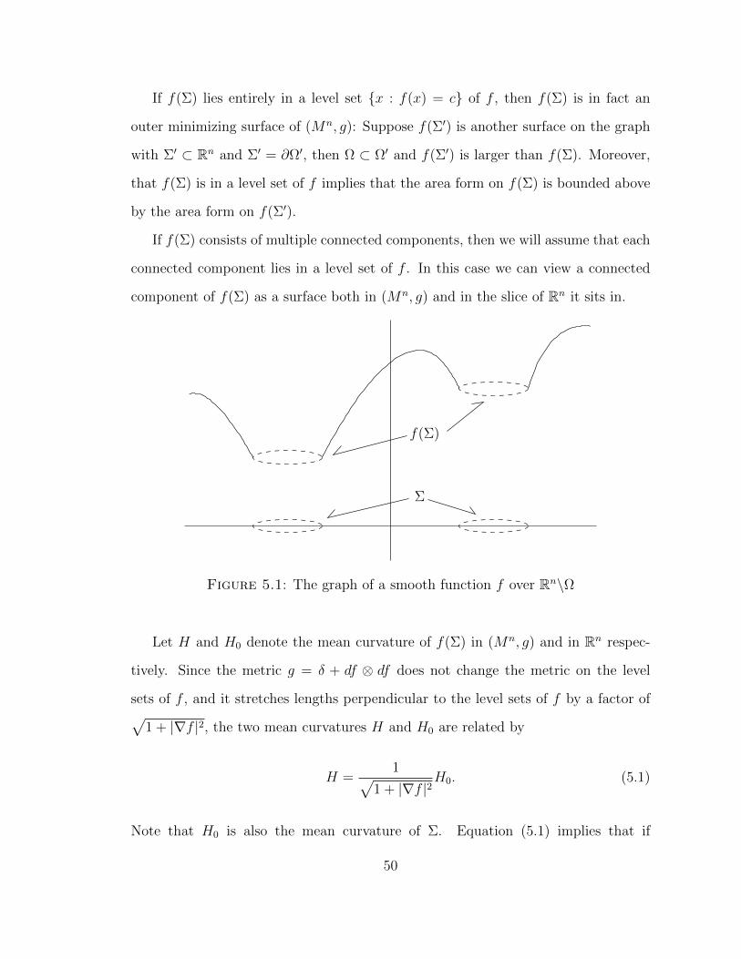
If f(Σ) lies entirely in a level set x : f(x) = c of f , then f(Σ) is in fact an

outer minimizing surface of (Mn, g): Suppose f(Σ′) is another surface on the graph

with Σ′ ⊂ Rn and Σ′ = ∂Ω′, then Ω ⊂ Ω′ and f(Σ′) is larger than f(Σ). Moreover,

that f(Σ) is in a level set of f implies that the area form on f(Σ) is bounded above

by the area form on f(Σ′).

If f(Σ) consists of multiple connected components, then we will assume that each

connected component lies in a level set of f . In this case we can view a connected

component of f(Σ) as a surface both in (Mn, g) and in the slice of Rn it sits in.

Σ

f(Σ)

Figure 5.1: The graph of a smooth function f over Rn\Ω

Let H and H0 denote the mean curvature of f(Σ) in (Mn, g) and in Rn respec-

tively. Since the metric g = δ + df ⊗ df does not change the metric on the level

sets of f , and it stretches lengths perpendicular to the level sets of f by a factor of√1 + |∇f |2, the two mean curvatures H and H0 are related by

H =1√

1 + |∇f |2H0. (5.1)

Note that H0 is also the mean curvature of Σ. Equation (5.1) implies that if

50

|∇f(x)| → ∞ as x → Σ, then f(Σ) is an outer minimizing horizon of (Mn, g)

since H ≡ 0 on Σ. Graphically, this means f is ‘vertical’ along the boundary.

Σ

f(Σ)

Figure 5.2: The graph of a smooth function f over Rn\Ω with minimal boundary

In this setting, proving Theorem 19 is a matter of keeping track of the extra

boundary term when we apply the divergence theorem in the proof of Theorem 12.

As before, any repeated indices are being summed over.

Proof of Theorem 19. As in the proof of Theorem 12, we can write the mass of

(Mn, g) as

mADM = limr→∞

1

2(n− 1)ωn−1

∫Sr

1

1 + |∇f |2(fiifj − fijfi)νjdSr.

The difference here is that when we apply the divergence theorem, we get an extra

51

boundary integral:

mADM = limr→∞

1

2(n− 1)ωn−1

∫Sr

1

1 + |∇f |2(fiifj − fijfi)νjdSr

= − 1

2(n− 1)ωn−1

∫Σ

1

1 + |∇f |2(fiifj − fijfi)νjdA

+1

2(n− 1)ωn−1

∫Rn\Ω∇ ·(

1

1 + |∇f |2(fiifj − fijfi)∂j

)dVδ,

where technically we cannot apply the divergence theorem to all of Rn\Ω since

|∇f(x)| → ∞ as x → ∂Ω = Σ. However, we will slightly abuse our notations

here since we will show later that the improper integrals do in fact converge. Thus

mADM = − 1

2(n− 1)ωn−1

∫Σ

1

1 + |∇f |2(fiifj − fijfi)νjdA

+1

2(n− 1)ωn−1

∫Mn

R1√

1 + |∇f |2dVg,

where we have rewritten the second integral using Lemma 14. The outward normal

to Mn along Σ is ν = ∇f/|∇f |. Viewing Σ as a closed surface in (Rn, δ), we denote

by ∆f the Laplacian of f with respect to the flat metric and ∆Σf the Laplacian of

f restricted along Σ. Let Hf denote the Hessian of f and H0 the mean curvature of

Σ with respect to the flat metric. We will use the following well known formula to

relate the two Laplacians:

∆f = ∆Σf +Hf (ν, ν) +H0 · ν(f)

=1

|∇f |Hf

(∇f, ∇f|∇f |

)+H0|∇f |,

(5.2)

52

where ∆Σf = 0 since f is constant on Σ. Now

− 1

1 + |∇f |2(fiifj − fijfi)νj

=1

1 + |∇f |2

[(∆f)|∇f | −Hf

(∇f, ∇f|∇f |

)]

=1

1 + |∇f |2

[(1

|∇f |Hf

(∇f, ∇f|∇f |

)+H0|∇f |

)|∇f | −Hf

(∇f, ∇f|∇f |

)]

=|∇f |2

1 + |∇f |2H0.

(5.3)

Therefore,

mADM =1

2(n− 1)ωn−1

∫Σ

|∇f |2

1 + |∇f |2H0dA+

1

2(n− 1)ωn−1

∫Mn

R1√

1 + |∇f |2dVg

=1

2(n− 1)ωn−1

∫Σ

H0dA+1

2(n− 1)ωn−1

∫Mn

R1√

1 + |∇f |2dVg.

Remark 22. Since f(Σ) is in a level set of f , it is the same surface as Σ translated

vertically. Thus we can equivalently express the ADM mass as

mADM =1

2(n− 1)ωn−1

∫f(Σ)

H0dA+1

2(n− 1)ωn−1

∫Mn

R1√

1 + |∇f |2dVg.

5.2 Aleksandrov-Fenchel inequality

Since the Penrose inequality bounds the ADM mass below by the mass of the black

hole, we would like to apply Theorem 19 to this setting. In dimension n = 3, Theorem

19 gives

mADM =1

16π

∫Σ

H0dA+1

16π

∫M3

R1√

1 + |∇f |2dVg.

53

Suppose for now that Σ is connected. If in addition we assume that Σ is the boundary

of a convex region, then a classical inequality in convex geometry states that

1

16π

∫Σ

H0dA ≥√

A

16π,

where A = |Σ| as usual. If this is the case, then Theorem 19 implies

mADM ≥√

A

16π+

1

16π

∫M3

R1√

1 + |∇f |2dVg ≥

√A

16π

assuming R ≥ 0, which is precisely the Riemannian Penrose inequality. In fact, the

above inequality is true in higher dimensions for a boundary whose connected com-

ponents are convex. The tool we need is the following lemma, which is a consequence

of the Aleksandrov-Fenchel inequality [20].

Lemma 23. If Σ is a connected convex surface in Rn with mean curvature H0 and

area |Σ|, then

1

2(n− 1)ωn−1

∫Σ

H0dA ≥1

2

(|Σ|ωn−1

)n−2n−1

.

Proof. Let Σ ⊂ Rn be a convex surface with principal curvatures κ1, . . . , κn−1. Let

σj(κ1, . . . , κn−1) =

(n− 1

j

)−1 ∑1≤i1<···<ik≤n−1

κi1 · · ·κij

be the jth normalized elementary symmetric functions in κ1, . . . , κn−1 for

j = 1, . . . , n− 1. In particular,

σ0(κ1, . . . , κn−1) = 1

σ1(κ1, . . . , κn−1) =1

n− 1

n−1∑i=1

κi =1

n− 1H0

σn−1(κ1, . . . , κn−1) =n−1∏i=1

κi.

54

The kth quermassintegral Vk of Σ is defined to be

Vk =

∫Σ

σk(κ1, . . . , κn−1).

A special case of the Aleksandrov-Fenchel inequality states that, for 0 ≤ i < j < k ≤

n− 1,

V k−1j ≥ V k−j

i V j−ik .

Taking i = 0, j = 1, k = n− 1,

V n−11 ≥ V n−2

0 Vn−1. (5.4)

Now

V0 =

∫Σ

σ0(κ1, . . . , κn−1) = |Σ|

V1 =

∫Σ

σ1(κ1, . . . , κn−1) =1

n− 1

∫Σ

H0

Vn−1 =

∫Σ

σn−1(κ1, . . . , κn−1) = ωn−1.

Thus (5.4) becomes (1

n− 1

∫Σ

H0

)n−1

≥ |Σ|n−2ωn−1

1

n− 1

∫Σ

H0 ≥ |Σ|n−2n−1ω

1n−1

n−1

1

2(n− 1)ωn−1

∫Σ

H0 ≥1

2

(|Σ|ωn−1

)n−2n−1

as claimed.

We can prove Corollary 20 using Theorem 19 and Lemma 23:

55

Proof of Corollary 20. Let us denote by Ωi, i = 1, . . . , k the connected, convex com-

ponents of the bounded open set Ω and let Σi = ∂Ωi. The ADM mass of (Mn, g)

is

mADM = limr→∞

1

2(n− 1)ωn−1

∫Sr

1

1 + |∇f |2(fiifj − fijfi)νjdSr

=k∑i=1

1

2(n− 1)ωn−1

∫Σi

H0dA+1

2(n− 1)ωn−1

∫Mn

R1√

1 + |∇f |2dVg

≥k∑i=1

1

2

(|Σi|ωn−1

)n−2n−1

+1

2(n− 1)ωn−1

∫Mn

R1√

1 + |∇f |2dVg

56

6

Graphs in Minkowski Space and the Mass of ZAS

Up to this point, we have assumed that the parameter m in the 3-dimensional

Schwarzschild manifold (R3\0, (1 + m2r

)4δ) is positive. If we consider the same

metric but with m < 0, then this gives a Riemannian metric on R3 minus a closed

ball of radius |m|/2 about the origin that approaches zero near its inner boundary.

In this case, one may think of the ‘point’ r = |m|/2 as a black hole of negative mass.

In fact, this metric has a naked singularity, that is, a singularity not enclosed by

any apparent horizon. Such singularity is called a zero area singularity (ZAS), and

the Schwarzschild manifold with negative mass is known as the Schwarzschild ZAS

manifold. We use our techniques from earlier chapters to study such manifolds that

are graphs in Minkowski space and we begin by defining the notion of ZAS, following

the approach of Bray and Jauregui [6].

6.1 The notion of zero area singularities

A zero area singularity is characterized by the property that nearby surfaces have

arbitrarily small area. More precisely,

57

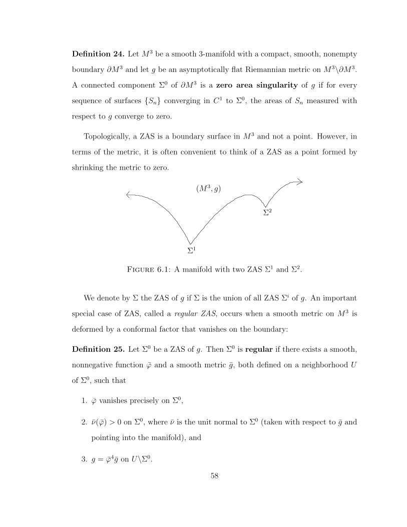
Definition 24. Let M3 be a smooth 3-manifold with a compact, smooth, nonempty

boundary ∂M3 and let g be an asymptotically flat Riemannian metric on M3\∂M3.

A connected component Σ0 of ∂M3 is a zero area singularity of g if for every

sequence of surfaces Sn converging in C1 to Σ0, the areas of Sn measured with

respect to g converge to zero.

Topologically, a ZAS is a boundary surface in M3 and not a point. However, in

terms of the metric, it is often convenient to think of a ZAS as a point formed by

shrinking the metric to zero.

(M3, g)

Σ1

Σ2

Figure 6.1: A manifold with two ZAS Σ1 and Σ2.

We denote by Σ the ZAS of g if Σ is the union of all ZAS Σi of g. An important

special case of ZAS, called a regular ZAS, occurs when a smooth metric on M3 is

deformed by a conformal factor that vanishes on the boundary:

Definition 25. Let Σ0 be a ZAS of g. Then Σ0 is regular if there exists a smooth,

nonnegative function ϕ and a smooth metric g, both defined on a neighborhood U

of Σ0, such that

1. ϕ vanishes precisely on Σ0,

2. ν(ϕ) > 0 on Σ0, where ν is the unit normal to Σ0 (taken with respect to g and

pointing into the manifold), and

3. g = ϕ4g on U\Σ0.

58

If such a pair (g, ϕ) exists, it is called a local resolution of Σ0.

An example of a regular ZAS is that of the Schwarzschild ZAS manifold

(M3, g) =(R3\B|m|/2, (1 +

m

2r)4δ)

for m < 0.

The boundary of M3 consists of a single connected component Σ = Σ0 = S|m|/2. It

is easy to check that ϕ = (1 + m2r

) and g = δ satisfy the conditions of Definition 25.

Moreover, this is in fact an example of a globally harmonic resolution of Σ, in the

sense that the factor ϕ is defined on all of M3\Σ and that ϕ is harmonic with respect

to g.

(R3\B|m|/2, (1 + m2r

)4δ)

Σ

Figure 6.2: The 3-dimensional Schwarzschild ZAS manifold.

We can now define the mass of a regular ZAS:

Definition 26. Let (g, ϕ) be a local resolution of a ZAS Σ0 of g. Then the regular

mass of Σ0 is defined by the flux integral

mreg(Σ0) = −1

4

(1

π

∫Σ0

ν(ϕ)4/3dA

)3/2

,

where ν is the unit normal to Σ0 (pointing into the manifold) and dA is the area

form induced by g.

As shown in [6], this definition

1. is independent of the choice of local resolution,

59

2. depends only on the local geometry of (M3, g) near Σ0,

3. is related to the Hawking masses of nearby surfaces,

4. arises naturally in the proof of the Riemannian ZAS inequality, and

5. equals m for the Schwarzschild ZAS metric of ADM mass m < 0.

And finally, we can define the mass of an arbitrary ZAS using regular mass:

Definition 27. Let Σ = ∂M3 be zero area singularities of (M3, g). The mass of Σ

is

mZAS(Σ) := supΣn

(lim supn→∞

mreg(Σn)

),

where the supremum is taken over all sequences Σn converging in C1 to Σ.

6.2 Graphs in Minkowski space

As we discussed in Chapter 3, the 3-dimensional Schwarzschild manifold with positive

mass can be isometrically embedded as a rotating parabola

r =w2

8m+ 2m

in flat R4, where r =√x2 + y2 + z2 and (x, y, z, w) are the standard coordinates on

R4. Now if m < 0, then solving for w2 gives

w2 = 8m(r − 2m).

Note that since m < 0, we cannot solve for w like we did before to get a graph in

Euclidean space. However, if we send w 7→ iw, then

(iw)2 = 8m(r − 2m)

−w2 = 8m(r − 2m)

w =√

8|m|(r − 2m)1/2

60

is once again a function w = f(r) on R3, where f is a smooth function for r > 0, that

is, when it is away from the singularity r = 0. Note that under the transformation

w 7→ iw, the underlying metric dx2 +dy2 +dz2 +dw2 on R4 becomes dx2 +dy2 +dz2−

dw2. In other words, we can embed the Schwarzschild ZAS manifold into Minkowski

space R3,1. Moreover, since

|∇f |2 =2|m|r − 2m

< 1 for r > 0,

a tangent vector to the Schwarzschild ZAS manifold has length greater than 0 in R3,1

and the Schwarzschild ZAS manifold is a spacelike slice of Minkowski space.

Motivated by this example, we can more generally consider functions on Rn whose

graph is a spacelike slice in Minkowski space Rn,1 with the induced metric. We will

assume that such functions are smooth outside any singularities. By an argument

similar to that in the proof of Proposition 6, the graph manifold (Mn, g) with the

induced metric g from Rn,1 is isometric to (Rn, δ− df ⊗ df). Thus we will henceforth

refer to (Rn, δ − df ⊗ df) as the graph of f (in Minkowski space).

We now proceed to compute the scalar curvature of such a graph (Mn, g) in

Minkowski space and hope that just like before, it is a divergence. First, the scalar

curvature is given by the following Proposition.

Proposition 28. The scalar curvature R of a spacelike graph (Rn, δ − df ⊗ df) in

Rn,1 is given by

R =1

1− |∇f |2

(fijfij − fiifjj +

2fjfk1 + |∇f |2

(fijfik − fiifjk)).

Proof. If gij = δij − fifj, then

gij = δij +f if j

1− |∇f |2,

61

since

gijgjk = (δij − fifj)

(δjk +

f jfk

1− |∇f |2

)

= δijδjk − fifjδjk + δij

f jfk

1− |∇f |2− fifj

f jfk

1− |∇f |2

= δki − fifk +fif

k(1− |∇f |2)

1− |∇f |2

= δki .

The Christoffel symbols of g are

Γkij =1

2gkm(gim,j + gjm,i − gij,m)

=1

2

(δkm +

fkfm

1− |∇f |2

)(−fijfm − fifjm − fijfm − fjfim + fimfj + fifjm)

=1

2

(δkm +

fkfm

1− |∇f |2

)(−2fijfm)

= −fijfk −fijf

k|∇f |2

1− |∇f |2

= − fijfk

1− |∇f |2.

Just like before, we will write all indices as lower indices and sum over all repeated

ones. Thus

Γkij = − fijfk1− |∇f |2

Γkij,k = − fijkfk1− |∇f |2

− fijfkk1− |∇f |2

− 2fijfklfkfl(1− |∇f |2)2

.

62

The scalar curvature R can now be computed as follows:

R = gij(Γkij,k − Γkik,j + ΓlijΓkkl − ΓlikΓ

kjl)

=

(δij +

fifj1− |∇f |2

)(− fijkfk

1− |∇f |2− fijfkk

1− |∇f |2− 2fijfklfkfl

(1− |∇f |2)2+

fijkfk1− |∇f |2

+fikfjk

1− |∇f |2+

2fikfjlfkfl(1− |∇f |2)2

+fijfklfkfl

(1− |∇f |2)2− fikfjlfkfl

(1− |∇f |2)2

)

=

(δij +

fifj1− |∇f |2

)(− fijfkk

1− |∇f |2+

fikfjk1− |∇f |2

− fijfklfkfl(1− |∇f |2)2

+fikfjlfkfl

(1− |∇f |2)2

)

=1

1− |∇f |2(fikfik − fiifkk) +

fkfl(1− |∇f |2)2

(fikfil − fiifkl)

+fifj

(1− |∇f |2)2(fikfjk − fijfkk)−

fifjfkfl(1− |∇f |2)3

(fijfkl − fikfjl).

Once again, the last term is 0 by symmetry, and relabeling the indices gives

R =1

1− |∇f |2

(fijfij − fiifjj +

2fjfk1 + |∇f |2

(fijfik − fiifjk)).

Now since gij = δij − fifj, we have

gij,i − gii,j = −fiifj − fifij + 2fijfi = fijfi − fiifj.

Motivated by our discussion of the ADM mass of a graph in Euclidean space, we give

an alternate definition of the ADM mass for a spacelike graph in Minkowski space

by multiplying the integrand in the ADM mass by the factor 1/(1− |∇f |2).

Definition 29. If (Mn, g) is the graph of an asymptotically flat function that is a

spacelike slice in Rn,1 with the induced metric, then the ADM mass of (Mn, g) is

mADM = limr→∞

1

2(n− 1)ωn−1

∫Sr

1

1− |∇f |2(fijfi − fiifj)νjdSr. (6.1)

63

Fortunately, the scalar curvature in this case is once again the divergence of the

above integrand:

Lemma 30. The scalar curvature R of the graph (Rn, δ − df ⊗ df) satisfies

R = ∇ ·(

1

1− |∇f |2(fijfi − fiifj)∂j

)

Proof. Now that we know what to look for, this lemma is once again a direct calcu-

lation:

∇ ·(

1

1− |∇f |2(fijfi − fiifj)∂j

)

=1

1− |∇f |2(fijjfi + fijfij − fiijfj − fiifjj) +

2fjkfk(1− |∇f |2)2

(fijfi − fiifj)

=1

1− |∇f |2

(fijfij − fiifjj +

2fjfk1− |∇f |2

(fijfik − fiifjk))

= R.

6.3 ZAS inequality for graphs in Minkowski space

We begin this section by giving an alternate definition of the mass of a ZAS for

spacelike graphs in Minkowski space.

Definition 31. Let (Mn, g) be the graph of a function f on Rn that is a spacelike slice

in Rn,1 with the induced metric. We say that Σ0 ∈ Mn is a zero area singularity

(ZAS) of (Mn, g) if the areas of a sequence of surfaces Σk, each Σk being in a

level set of f , converge to 0 and Σk converges to Σ0.

If Σi, i = 1, . . . ,m are all the zero area singularities of (Mn, g), then we denote

by Σ the (disjoint) union of all the Σi.

64

To motivate our definition of the mass of a ZAS, let us for now assume that the

ZAS of (Mn, g) consists of only one connected component Σ0 (that is, a single point).

Let Σk be a sequence of surfaces, each of which is in a level set of f , such that

Σk converges to Σ0 and let Σk = ∂Ωk. If we apply the divergence theorem to (6.1)

and use Lemma 30, then for a given k,

mADM = limr→∞

1

2(n− 1)ωn−1

∫Sr

1

1− |∇f |2(fijfi − fiifj)νjdSr.

=1

2(n− 1)ωn−1

∫Rn\Ωk

∇ ·(

1

1− |∇f |2(fijfi − fiifj)∂j

)dVδ

− 1

2(n− 1)ωn−1

∫Σk

1

1− |∇f |2(fijfi − fiifj)νjdA

=1

2(n− 1)ωn−1

∫Mn\f(Ωk)

R1√

1− |∇f |2dVg

− 1

2(n− 1)ωn−1

∫Σk

|∇f |2

1− |∇f |2H0dA,

where the last equality follows from the fact that νj = ∇f/|∇f | and

(fijfi − fiifj)νj = Hf

(∇f, ∇f|∇f |

)− (∆f)∇f · ∇f

|∇f |

= Hf

(∇f, ∇f|∇f |

)−∆f |∇f |

= Hf

(∇f, ∇f|∇f |

)−[Hf

(∇f, ∇f|∇f |

)+H0|∇f |

]|∇f |

= H0|∇f |2

using (5.2).

Once again, we can view the ADM mass as the sum of the mass contribution from

the local energy density over Mn and the mass of the surface Σk. Because of this,

and motivated by the standard definition of a ZAS, we make the following definition:

65

Definition 32 (Mass of ZAS, single component). Let Σk be a sequence of surfaces

in Mn, each being in a level set of f , such that Σk converges to Σ0. Then we define

mZAS(Σ0) = limk→∞− 1

2(n− 1)ωn−1

∫Σk

|∇f |2

1− |∇f |2H0dA.

If the ZAS Σ of (Mn, g) consists of multiple connected components Σi, i =

1, . . . ,m, then we define the mass of the ZAS as the sum of the masses of the

components.

Definition 33 (Mass of ZAS).

mZAS(Σ) =k∑i=1

mZAS(Σi)

We can now state and prove the ZAS inequality for graphs in Minkowski space.

Theorem 34 (ZAS inequality for graphs). Let (Mn, g) be the graph of an asymp-

totically flat function in Minkowski space Rn,1 with the induced metric. Let R be

the scalar curvature of g and mADM its ADM mass. Suppose Σi, i = 1, . . . ,m are

the connected components of the ZAS Σ of (Mn, g) such that Σik are the surfaces

converging to Σi. Let Σik = ∂Ωi

k and denote by Ωk = ∪mi=1Ωik. Then the ADM mass

of (Mn, g) satisfies

mADM = limk→∞

1

2(n− 1)ωn−1

∫Mn\f(Ωk)

R1√

1− |∇f |2dVg +mZAS(Σ).

In particular, if R ≥ 0, then we have the usual ZAS inequality

mADM ≥ mZAS(Σ).

66

Proof of Theorem 34. Applying the divergence theorem to (6.1),

mADM = limr→∞

1

2(n− 1)ωn−1

∫Sr

1

1− |∇f |2(fijfi − fiifj)νjdSr.

= limk→∞

1

2(n− 1)ωn−1

∫Mn\f(Ωk)

R1√

1− |∇f |2dVg

− limk→∞− 1

2(n− 1)ωn−1

∫Σk

|∇f |2

1− |∇f |2H0dA

= limk→∞

1

2(n− 1)ωn−1

∫Mn\f(Ωk)

R1√

1− |∇f |2dVg +mZAS(Σ).

67

7

A New Quasi-Local Mass

Let (Mn, g) be the graph of a smooth function on Rn and let Σ ⊂ Rn be a closed

surface such that f(Σ) ⊂ Mn is in a level set of f . Let H be the mean curvature

of Σ in (Mn, g) and let H0 be the mean curvature of Σ in (Rn, δ). We define the

quasi-local mass of the surface f(Σ) to be

mQL(f(Σ)) =1

2(n− 1)ωn−1

∫f(Σ)

1

H0

(H20 −H2)dA

and show that this definition of mass is nonnegative, monotonically nondecreasing

and approaches the ADM mass of (Mn, g) at ∞.

In dimension n = 3, we can define the masses of closed surfaces in more general

manifolds besides those that are graphs. If (M3, g) is a complete, asymptotically

flat manifold with nonnegative scalar curvature and Σ is a closed surface in (M3, g)

with Gauss curvature K > 0, then the Weyl embedding theorem [17] implies that Σ

can be isometrically embedded into R3. Moreover, the embedding is unique up to an

isometry of R3. Let H be the mean curvature of Σ in (M3, g) and let H0 be the mean

curvature of Σ in R3 under the isometric embedding. We define a new quasi-local

68

mass functional of Σ by

mQL(Σ) =1

16π

∫Σ

1

H0

(H20 −H2)dA.

We give the motivation for our definition of quasi-local mass and study some of its

properties in this chapter.

7.1 On quasi-local mass functionals

As we noted in Chapter 1, the 3-dimensional Schwarzschild manifold is the equality

case of the Riemannian Penrose inequality with

mADM =

√A

16π,

where A is the area of the outermost minimal surface corresponding to the apparent

horizon of a black hole. Since the Schwarzschild manifold is scalar flat, it has zero

local energy density everywhere and one can view the mass contribution as coming

solely from the black hole. Therefore it is natural to consider the quantity√A/16π

as the mass of a black hole of area A. More generally, given any bounded region Ω

with smooth boundary Σ = ∂Ω in a complete, asymptotically flat manifold (M3, g),

we would like to define how much mass Ω (or equivalently, Σ) possesses. Assuming

(M3, g) has nonnegative scalar curvature (local energy density) everywhere, there are

certain reasonable properties one would expect from such quasi-local mass functional

m(Σ), most notably [4, 11],

1. (nonnegativity) m(Σ) ≥ 0;

2. (rigidity/strict positivity) m(Σ) = 0 if and only if Σ is flat;

3. (monotonicity) m(Σ1) ≤ m(Σ2) if Σ1 = ∂Ω1 and Σ2 = ∂Ω2 with Ω1 ⊂ Ω2;

69

4. (ADM limit) m(Σ) should be asymptotic to the ADM mass, that is, if Σk is

a sequence of surfaces that exhaust (M3, g), then

limk→∞

m(Σk) = mADM(g);

5. (black hole limit) m(Σ) should agree with the black hole mass, that is, if Σ

is a horizon in (M3, g), then

m(Σ) =

√A

16π,

where A is the area of Σ.

There have been numerous attempts to define such quasi-local mass functionals

[3, 4, 5, 9, 10, 13, 27], but to date, none of them satisfy all of the properties listed

above. For example, as discussed in Chapter 2, the Hawking mass

mH(Σ) =

√|Σ|16π

(1− 1

16π

∫Σ

H2dA

)

is monotonically nondecreasing under inverse mean curvature flow, and that its

asymptotic limit coincides with the ADM mass. Moreover, it gives the correct black

hole mass if Σ is a horizon, as H ≡ 0 along Σ. Thus the Hawking mass satisfies the

last three properties listed above, with monotonicity in the sense of inverse mean

curvature flow.

Unfortunately, the Hawking mass does not satisfy the first two properties. In fact,

mH(Σ) ≤ 0 for any closed surface Σ in R3. Nevertheless, it is known that mH ≥ 0

for a stable constant mean curvature 2-sphere in a 3-manifold of nonnegative scalar

curvature [11].

Another notable example of a quasi-local mass functional is the Brown-York mass

[9, 10]. If Σ ⊂ M3 is a closed surface with positive Gauss curvature, then by the

70

Weyl embedding theorem [17], it can be isometrically embedded into R3. Moreover,

the embedding is unique up to an isometry of R3. Let H be the mean curvature of Σ

in (M3, g) and let H0 be the mean curvature in R3 under the isometric embedding.

The Brown-York mass of Σ is defined to be

mBY (Σ) =1

8π

∫Σ

H0 −HdA,

where dA is the area element on Σ induced by g. In 2002, Shi and Tam [26] proved

that the Brown-York mass is nonnegative using a gluing argument by solving a

parabolic partial differential equation of a certain foliation and applying the positive

mass theorem.

While the Brown-York mass is nonnegative, it tends to overestimate the mass

of a given region. For example, the isometric image in R3 of the horizon in the

3-dimensional Schwarzschild manifold (M3, g) = (R3\0, (1 + m2r

)4) is the sphere

Σ = S2m of radius 2m. Thus H0 = 2/2m = 1/m and H = 0 and

mBY (Σ) =1

8π

∫Σ

H0 −HdA =1

8π· 4π(2m)2 · 1

m= 2m,

but the mass of the horizon should be m in this case. More generally, for a sphere

Sr in (M3, g), its isometric image in R3 is Sru2 with u = 1 + m2r

. Thus

H0 =2

ru2and H =

1

u2

(2

r+

4

u

∂u

∂r

).

71

The Brown-York mass of Sr is then

mBY (Sr) =1

8π

∫Sr

H0 −HdA

=1

8π· 4πr2u4 ·

[2

ru2− 1

u

(2

r+

4

u

∂u

∂r

)]

= −2r2u∂u

∂r

= −2r2u(− m

2r2

)= m

(1 +

m

2r

).

Thus mBY (Sr) is actually monotonically decreasing to the ADM mass as r →∞ in

the Schwarzschild manifold.

7.2 Motivation for the definition of mQL

In Chapter 5, we considered the graph (Mn, g) of a smooth function f : Rn\Ω→ R,

where Ω is a bounded open set in Rn with smooth boundary Σ = ∂Ω. If we in

addition assume that f(Σ) is a minimal boundary of (Mn, g) that is contained in a

level set of f , then Theorem 19 states that

mADM(g) =1

2(n− 1)ωn−1

∫f(Σ)

H0dA+1

2(n− 1)ωn−1

∫Mn

R1√

1 + |∇f |2dVg,

where H0 is the mean curvature with respect to the flat metric. One can view the

above as an expression of the ADM mass of the manifold as the sum of the mass

of the boundary and the mass contribution from the local energy density over the

manifold.

If we remove the assumption that f(Σ) is minimal, equation (5.3) implies that

the boundary integral is

1

2(n− 1)ωn−1

∫f(Σ)

|∇f |2

1 + |∇f |2H0dA. (7.1)

72

Recall that equation (5.1) relates the mean curvatures H and H0 by

H =1√

1 + |∇f |2H0,

which we can rewrite as (H

H0

)2

=1

1 + |∇f |2

1−(H

H0

)2

=|∇f |2

1 + |∇f |2.

Thus equation (7.1) can be expressed as

1

2(n− 1)ωn−1

∫f(Σ)

|∇f |2

1 + |∇f |2H0dA =

1

2(n− 1)ωn−1

∫f(Σ)

[1−

(H

H0

)2]H0dA

=1

2(n− 1)ωn−1

∫f(Σ)

1

H0

(H20 −H2)dA.

(7.2)

Because of (7.2), we make the following definition:

Definition 35. Let (Mn, g) be the graph of a smooth asymptotically flat function

f : Rn → R with the induced metric g from Rn+1. If Σ ⊂ Rn is a closed surface such

that f(Σ) ⊂Mn is in a level set of f , then we define the quasi-local mass of Σ to be

mQL(f(Σ)) =1

2(n− 1)ωn−1

∫f(Σ)

1

H0

(H20 −H2)dA.

Moreover, if Ω is a bounded set in Rn such that ∂Ω = Σ, then the divergence

theorem implies that

mQL(f(Σ)) =1

2(n− 1)ωn−1

∫f(Σ)

1

H0

(H20 −H2)dA

=1

2(n− 1)ωn

∫f(Ω)

R1√

1 + |∇f |2dVg.

(7.3)

We can view (7.3) as an alternate characterization of the mass of f(Σ).

73

7.3 Properties of mQL

We collect the properties of mQL in the following theorem:

Theorem 36. Let (Mn, g) be the graph of a smooth asymptotically flat function

f : Rn → R with nonnegative scalar curvature. Let Σ ⊂ Rn be a closed surface such

that f(Σ) ⊂Mn is in a level set of f . Let H and H0 denote its mean curvature with

respect to g and the flat metric respectively. The quasi-local mass functional

mQL(f(Σ)) =1

2(n− 1)ωn−1

∫f(Σ)

1

H0

(H20 −H2)dA

satisfies

1. (Nonnegativity) mQL(f(Σ)) ≥ 0,

2. (Monotonicity) If Σ1 = ∂Ω1 and Σ2 = ∂Ω2 are such that Ω1 ⊂ Ω2, then

mQL(f(Σ1)) ≤ mQL(f(Σ2)).

3. (ADM limit) If Σk is a sequence that exhausts Rn, then

limk→∞

mQL(f(Σk)) = mADM(g).

Proof. 1. is an immediate consequence of (7.3) since

mQL(f(Σ)) =1

2(n− 1)ωn−1

∫f(Ω)

R1√

1 + |∇f |2dVg > 0

and R ≥ 0 by assumption. Thus mQL(f(Σ)) satisfies nonnegativity.

If Σ1 and Σ2 are such that Σ1 = ∂Ω1, Σ2 = ∂Ω2 with Ω1 ⊂ Ω2, then

mQL(f(Σ1)) =1

2(n− 1)ωn−1

∫f(Ω1)

R1√

1 + |∇f |2dVg

≤ 1

2(n− 1)ωn−1

∫f(Ω2)

R1√

1 + |∇f |2dVg = mQL(f(Σ2))

74

using R ≥ 0.

Finally, if Σk is a sequence of surfaces that exhaust Rn, then we can express

the ADM mass of (Mn, g) as

mADM = mQL(f(Σk)) +1

2(n− 1)ωn−1

∫Mn\f(Ωk)

R1√

1 + |∇f |2dVg.

For each k. As k →∞, the second integral approaches 0 and thus mQL is asymptotic

to the ADM mass.

7.4 mQL for more general manifolds

In the previous section we showed that mQL is nonnegative, monotonically nonde-

creasing and asymptotic to the ADM mass for closed surfaces in complete graph

manifolds. We point out in this section that mQL can in fact be defined in more

general settings, namely, that whenever the Brown-York mass is defined. Suppose

(M3, g) is a complete, asymptotically flat manifold with nonnegative scalar curva-

ture and let Σ be a closed surface in (M3, g). If each connected component of Σ has

positive Gauss curvature, then Σ can be isometrically embedded in R3 by the Weyl’s

embedding theorem, and that the embedding is unique up to an isometry of R3. Let

H be the mean curvature of Σ in (M3, g) and let H0 be the mean curvature of Σ

when isometrically embedded into R3, then we define the quasi-local mass of Σ to be

mQL(Σ) =1

16π

∫Σ

1

H0

(H20 −H2)dA.

Since

mQL(Σ) =1

16π

∫Σ

1

H0

(H20 −H2)dA =

1

16π

∫Σ

H0 −HH

H0

dA,

75

mQL looks strikingly similar to the Brown-York mass mBY . In fact,

mBY (Σ)−mQL(Σ) =1

8π

∫Σ

H0 −HdA−1

16π

∫Σ

H0 −H2

H0

=1

16π

∫Σ

2H0 − 2H −H0 +H2

H0

dA

=1

16π

∫Σ

1

H0

(H −H0)2dA

≥ 0.

Therefore, by [26], we have

mBY (Σ) ≥ mQL(Σ) ≥ 0,

and that equality holds if and only if Ω is isometric to a domain in R3.

76

Bibliography

[1] R. Arnowitt, S. Deser, and C. Misner. Coordinate invariance and energy ex-pressions in general relativity. Phys. Rev., 122:997–1006, 1961.

[2] R. Bartnik. The mass of an asymptotically flat manifold. Comm. Pure Appl.Math., 39:661–693, 1986.

[3] R. Bartnik. New definition of quasilocal mass. Phys. Rev. Lett., 62:2346–2348,1989.

[4] R. Bartnik. Mass and 3-metrics of non-nonnegative scalar curvature. Proceedingsof the International Congress of Mathematicians, II:231–240, 2002.

[5] H. Bray. Proof the Riemannian Penrose inequality using the positive masstheorem. J. Differential Geom., 59:177–267, 2001.

[6] H. Bray and J. Jauregui. A geometric theory of zero area singularities in generalrelativity. http://arxiv.org/abs/0909.0522v1, 2009.

[7] H. Bray and M. Khuri. P.d.e’s which imply the Penrose conjecture. 2009.

[8] H. Bray and D. Lee. On the Riemannian Penrose inequality in dimensions lessthan 8. http://arxiv.org/abs/0705.1128v1, 2007.

[9] J.D. Brown and J. W. York. Quasilocal energy in general relativity. Contemp.Math., 132:129–142, 1992.

[10] J.D. Brown and J. W. York. Quasilocal energy and conserved charges derivedfrom the gravitational action. Phys. Rev. D (3), 47 (no. 4):1407–1419, 1993.

[11] D. Christodoulou and S.-T. Yau. Some remarks on quasi-local mass. Contemp.Math., 71:9–14, 1988.

[12] R. Geroch. Energy extraction. Ann. New York Acad. Sci., 224:108–117, 1973.

[13] S. Hawking. Gravitational radiation in an expanding universe. J. Math. Phys.,pages 9:598–604, 1968.

77

[14] G. Huisken and T. Ilmanen. The inverse mean curvature flow and the Rieman-nian Penrose inequality. J. Differential Geom., 59:353–437, 2001.

[15] P.S. Jang and R. Wald. The positive energy conjecture and the cosmic censorhypothesis. J. Math. Phys., 18:41–44, 1977.

[16] M.-K. George Lam. The graph cases of the Riemannian positive mass andPenrose inequalities in all dimensions. http://arxiv.org/abs/1010.4256v1, 2010.

[17] L. Nirenberg. The Weyl and Minkowski problems in differential geometry in thelarge. Comm. Pure Appl. Math, 6:337–394, 1953.

[18] B. O’Neill. Semi-Riemannian geometry with applications to relativity. AcademicPress, 1983.

[19] R. Penrose. Naked singularities. Ann. New York Acad. Sci., 224:125–134, 1973.

[20] R. Schneider. Convex bodies: the Brunn-Minkowski theory. Cambridge Univer-sity Press, 1993.

[21] R. Schoen. Variational theory for the total scalar curvature functional for Rie-mannian metrics and related topics. Topics in the calculus of variations, lecturenotes in math., 1365, 1987.

[22] R. Schoen and S.-T. Yau. On the proof of the positive mass conjecture in generalrelativity. Comm. Math. Phys., 65:45–76, 1979.

[23] R. Schoen and S.-T. Yau. On the structure of manifolds with positive scalarcurvature. Manuscripta Math., 28(1-3):159–183, 1979.

[24] R. Schoen and S.-T. Yau. Proof of the positive mass theorem. ii. Comm. Math.Phys., 79:231–260, 1981.

[25] F. Schwartz. A volumetric Penrose inequality for conformally flat manifolds.http://arxiv.org/abs/1009.1587v2, 2010.

[26] Y. Shi and L.-F. Tam. Positive mass theorem and the boundary behaviors ofcompact manifolds with nonnegative scalar curvature. J. Diff. Geom., 62:79–125, 2002.

[27] Y. Shi and L.-F. Tam. Quasi-local mass and the existence of horizons. Comm.Math. Phys., 274:277–295, 2007.

[28] E. Witten. A new proof of the positive energy theorem. Comm. Math. Phys.,80:381–402, 1981.

78

Biography

Mau-Kwong George Lam was born in Hong Kong on February 1, 1983. He came

to the United States as a teenager and received a combined B.S./M.S.E. degree in

Applied Mathematics and Stattistics from Johns Hopkins University in Baltimore,

Maryland in May 2005. He had been at Duke University in Durham, North Carolina

since the Fall of 2005 and had received his Ph.D. and M.A. degrees in mathematics.

79