Chapter 3

The Gross-Pitaevskii equation

Learning goals

• What is the scattering cross-section?• How to describe the interaction between many atoms with a mean field potential.• Derivation and discussion of the Gross-Pitaevskii equation.• What is the Thomas-Fermi approximation?

3.1 Overview

So far we have looked at the interactions between two individual particles and found that –for low energies – the scattering properties can be described by a single number, the scatteringlength a. The e↵ective potential in this problem was then reduced to the pseudo potentialVpseudo

= 4⇡~2am �(r). This forms the basis of this chapter in which we aim to describe the

interaction between all particles in a Bose-Einstein condensate. After a short introduction tothe influence of quantum statistics onto the scattering cross section we move to the formulationof an e↵ective potential, the mean field potential, formed due to the presence of many atoms.To describe the resulting wave function of a BEC we derive the Gross-Pitaevskii equation andmake an important simplification, taking the Thomas-Fermi limit.This chapter is based on the Varenna lectures of Jean Dalibard (Collisional dynamics of ultra-cold atomic gases, 1998), on the Les Houches lectures of Yvan Castin (Bose-Einstein condensatesin atomic gases: simple theoretical results, 1999), arXiv:cond-mat/0105058, and on the bookAdvances in Atomic Physics by C. Cohen-Tannoudji and D. Guery-Odelin.

3.2 Scattering cross section

The scattering amplitude f(k, r) can be used to define a scattering cross section. For a sphericallysymmetric scattering potential, V (r) = V (r), one can write f(k, r) ! f(k,⇥). The di↵erentialscattering cross section, defined as the probability to find a scattered particle in the solid angled⌦ is then

d�

d⌦= |f(k,⇥)|2 . (3.1)

Integration overRd⌦ yields the total scattering cross section which – again taking the limit of

very low energies as in the previous chapter – only depends on the scattering length a,

�tot

k!0

= 4⇡a2 . (3.2)

We so far considered the scattering of distinguishable particles. This allows us to distinguishbetween the two situations shown in Figure 3.1, where the scattering amplitude is given by

18

either f(k,⇥), or by f(k,⇡ � ⇥). The situation changes if we now consider indistinguishableparticles. As shown in the two scattering diagrams, the two corresponding scattering amplitudescan not be distinguished any more because the wave packets overlap in the scattering region.The two-body wave functions have to be either symmetric (bosons) or antisymmetric (fermions),and the resulting scattering amplitude thus has to be rewritten as f(⇥)± f(⇡ �⇥), for bosons(+) respectively for fermions (-). As consequence, the di↵erential scattering cross sections andtotal cross sections become (again in the limit k ! 0)

d�

d⌦= |f(⇥)± f(⇡ �⇥)|2

Rd⌦

�!⇢

�bosons

= 8⇡a2

�fermions

= 0, (3.3)

where the integral has to be carried out only in the interval ⇥ 2 [0,⇡/2[ in order not to overcountterms.

Figure 3.1: Scattering of indistinguishable particles. The two possible ways in which twoindistinguishable particles can scatter lead to the final state. The scattering amplitudes have tobe added according to the quantum statistics of the particles.

This is a remarkable result: The scattering of indistinguishable bosons is enhanced with respectto the classical case, while the scattering of fermions is completely suppressed in the limit ofvery low energies. As a consequence, the evaporative cooling of a spin polarized fermionic gasis impossible and di↵erent experimental techniques have to be applied.

3.3 Mean-field energy and e↵ective refractive index

How can the interactions in a BEC be theoretically modeled? A starting point is to considerthe change in the wave function of a single particle due to its collisions with other particles. Forthis discussion we assume to be in the dilute limit, where the inter-particle distance is alwaysmuch larger than the scattering length, n|a|3 ⌧ 1, and we assume that the gas is at ultralowtemperatures, such that all scattering properties can be cast into the scattering length a (i.e.only s-wave scattering takes place). As shown in Fig. 3.2, we consider a particle with positionrp and momentum ~kp = zkp traveling along the z-direction. At z = 0, the atom enters a slabof of thickness L consisting of other atoms. The scattering at a single atom inside the slab atrest (k

1

= 0) at position r1

is described in relative coordinates r and k by

(r) / eikr � a

reikr . (3.4)

The scattering state in the laboratory frame can thus be expressed as the product of center-of-mass motion and relative motion,

lab

(rp, r1) = com

(r) (r) = eikcomrcom⇣eikr � a

reikr

⌘(3.5)

= eikpzp � a

|rp � r1

|eik

p

2|r

p

�r1|eik

p

2(z

p

+z1) . (3.6)

19

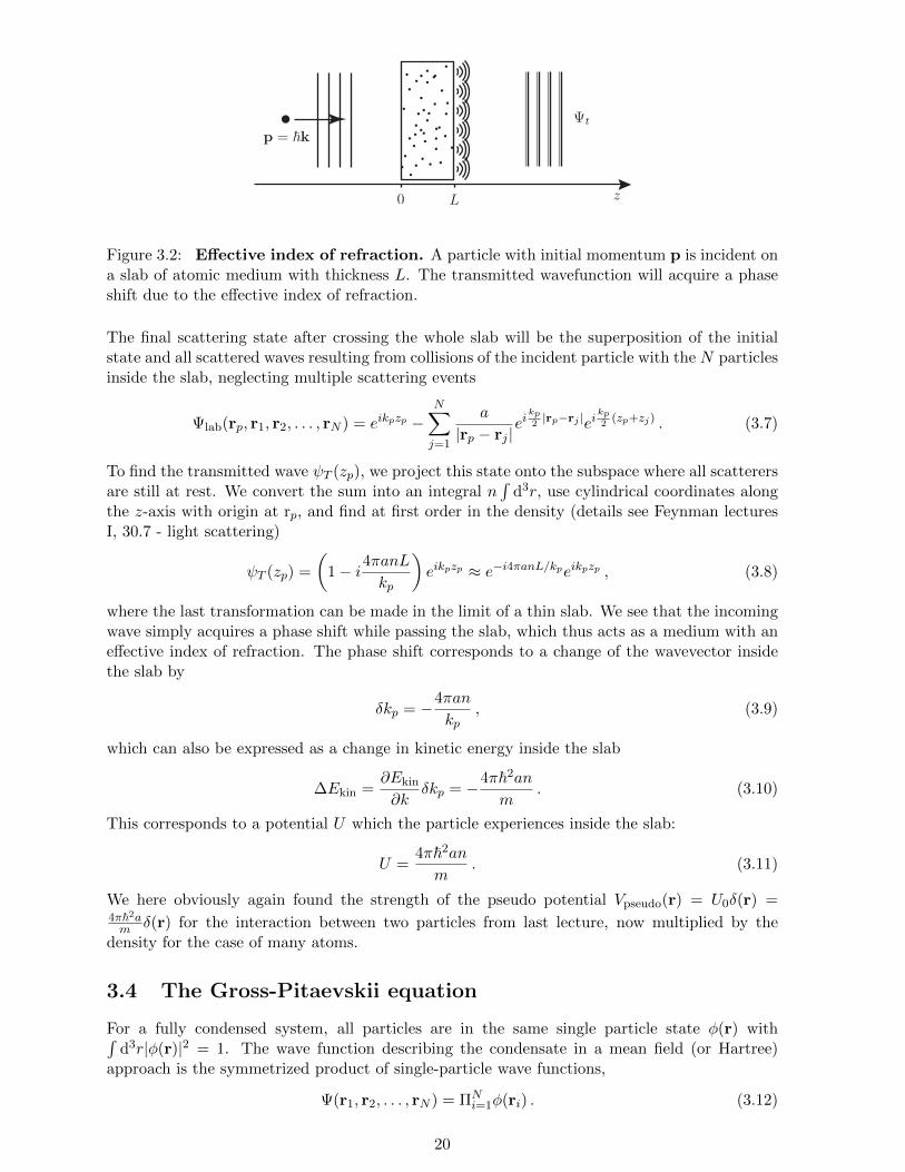
Figure 3.2: E↵ective index of refraction. A particle with initial momentum p is incident ona slab of atomic medium with thickness L. The transmitted wavefunction will acquire a phaseshift due to the e↵ective index of refraction.

The final scattering state after crossing the whole slab will be the superposition of the initialstate and all scattered waves resulting from collisions of the incident particle with the N particlesinside the slab, neglecting multiple scattering events

lab

(rp, r1, r2, . . . , rN ) = eikpzp �NX

j=1

a

|rp � rj |ei

k

p

2|r

p

�rj

|eik

p

2(z

p

+zj

) . (3.7)

To find the transmitted wave T (zp), we project this state onto the subspace where all scatterersare still at rest. We convert the sum into an integral n

Rd3r, use cylindrical coordinates along

the z-axis with origin at rp, and find at first order in the density (details see Feynman lecturesI, 30.7 - light scattering)

T (zp) =

✓1� i

4⇡anL

kp

◆eikpzp ⇡ e�i4⇡anL/k

peikpzp , (3.8)

where the last transformation can be made in the limit of a thin slab. We see that the incomingwave simply acquires a phase shift while passing the slab, which thus acts as a medium with ane↵ective index of refraction. The phase shift corresponds to a change of the wavevector insidethe slab by

�kp = �4⇡an

kp, (3.9)

which can also be expressed as a change in kinetic energy inside the slab

�Ekin

=@E

kin

@k�kp = �4⇡~2an

m. (3.10)

This corresponds to a potential U which the particle experiences inside the slab:

U =4⇡~2an

m. (3.11)

We here obviously again found the strength of the pseudo potential Vpseudo

(r) = U0

�(r) =4⇡~2am �(r) for the interaction between two particles from last lecture, now multiplied by the

density for the case of many atoms.

3.4 The Gross-Pitaevskii equation

For a fully condensed system, all particles are in the same single particle state �(r) withRd3r|�(r)|2 = 1. The wave function describing the condensate in a mean field (or Hartree)

approach is the symmetrized product of single-particle wave functions,

(r1

, r2

, . . . , rN ) = ⇧Ni=1

�(ri) . (3.12)

20

This wave function will be influenced by the kinetic energy, the potential energy and the in-teraction energy. The latter is taken into account via the mean field energy U

0

= 4⇡~2am which

(N � 1) particles create for one. The corresponding Hamiltonian then reads

H =NX

i=1

✓p2

i

2m+ V (ri)

◆+ U

0

X

i<j

�(ri � rj) . (3.13)

Using this Hamiltonian to find the according wave function of the BEC is a very hard problem.Instead, we can make use of a variational approach. We assume the condensate wavefunction tobe (r) =

pN�(r), and the according particle density to be n(r) = | (r)|2. Neglecting terms on

the order of 1/N which is save for large atom numbers, the energy functional for the N -particlewave function is given by

E(�,�⇤) = N

Zd3r

✓~22m

|r�(r)|2 + V (r)|�(r)|2 + 1

2NU

0

|�(r)|4◆

(3.14)

A solution for the wave function can now be found by minimizing this energy functional undervariations of � with the constraint

Rd3r|�(r)|2 = 1, i.e. that the total number of atoms stays

constant. The calculus can be carried out with the help of a Lagrange multiplier µ:

X(�,�⇤) = E(�,�⇤)� µN

Zd3r|�(r)|2 . (3.15)

We now need to find the minimum in the variation of X, i.e. �X = 0, due to variations of thewave function �! �+ ��. We find for �X 1

�X = N

Zd3r

✓~22m

r�r��⇤ + V (r)���⇤ +NU0

|�|2���⇤ � µ���⇤◆+ c.c. (3.16)

The wave function will have an imaginary and a real part. The variations in both parts shouldbe regarded as independent, which means that �X has to vanish independently for �� and ��⇤.We thus find2

✓� ~22m

r2 + V (r) + U0

| (r)|2◆ (r) = µ (r) , (3.17)

where we introduced for convenience the wave function (r) = N1/2�(r) of the condensate.Equation (3.17) is the time-independent Gross-Pitaevskii equation (GPE). It is a type of non-linear Schrodinger equation, where the total potential consists of the external potential V (r) anda non-linear term U

0

| (r)|2 which describes the mean-field potential of the other atoms. Theeigenvalue µ is the chemical potential. Note that it di↵ers from the mean energy per particleE/N as it would be found for a linear equation.If we consider a homogeneous, interacting gas, the GPE reduces to U

0

| (r)|2 = µ, i.e. µ = nU0

.This result can also be found using the thermodynamic relation µ = @E/@N with E = U

0

/V ·N(N � 1)/2 ⇡ U

0

/V ·N2/V .

3.5 The Thomas-Fermi approximation

We have seen that the full many-particle system can be reduced to the problem of finding a singleparticle, or condensate, wave function. The Gross-Pitaevskii equation determines the shape ofthis wave function. While being a tremendous simplification with respect to the original problem,it is still a non-linear Schrodinger equation to which we have generically no exact solution. Inthis section we learn how to simplify the full Gross-Pitaevskii equation in the presence of a trap.

1using r(�+ ��)r(�⇤ + ��⇤) = |r�|2 +r�r��⇤ +r�⇤r��+r��r��⇤ and(�+ ��)�⇤ + ��⇤) = |�|2 + ���⇤ + �⇤��+ ����⇤ and using only terms linear in the variations ��.

2We first apply a partial integration of the kinetic energy to get the same expression ���⇤ as in the otherterms. Then we set the full integrant to zero.

21

The equation we try to solve is given by

µ (r) =

� ~22m

r2 + V (r) + U0

| (r)|2� (r). (3.18)

Let us consider a harmonic potential

V (r) =m!2

0

2r2. (3.19)

By assuming a cloud of size ⇠ we can estimate both the average kinetic as well as the averagepotential energy per particle

Ekin ⇠ ~22m⇠2

, (3.20)

V ⇠ m!2

0

2⇠2. (3.21)

Owing to the virial theorem we can equate the two to find the typical cloud size for U0

= 0

⇠ =

r~

m!0

. (3.22)

Of course we would have obtained the same radius by solving the harmonic oscillator problemfor (r) given that U

0

= 0.

Let us now consider the influence of the interaction energyassuming that we have a typical particle density n = N/⇠3,where N denotes the number of particles. We find for theaverage interaction energy per particle

Eint ⇠ U0

n ⇠ U0

N

⇠3. (3.23)

Comparing this to the estimate of the kinetic energy (3.20) we see that in a trap, both theinteraction as well as the kinetic energy work in the same direction, i.e., both try to expand thecloud! Owing to this we can try to neglect the weaker of the two without picking up too muchof an error. If we compare kinetic and interaction energies we see that if U

0

exceeds the criticalstrength

U crit0

⇠ ~!0

2n(3.24)

we can neglect the kinetic term. This approximation is called the Thomas-Fermi approximation.3

Using the Thomas-Fermi approximation we can estimate the typical cloud size in the presenceof interaction R

@R

✓m!2

0

2R2 + U

0

N

R3

◆= m!2

0

R� 3U0

N1

R4

!

= 0. (3.25)

Therefore we obtain

R ⇠✓NU

0

m!2

0

◆1/5

⇠ ⇠

✓Na

⇠

◆1/5

, (3.26)

3The fact that both work in the same direction is absolutely essential in this step. Remember that the Gross-Pitaevskii equation is based on weak interactions. If the e↵ect of interactions would oppose the one of the kineticenergy, we could not skip the latter without violating the underlying assumption of weak interactions.

22

where we replaced the interaction constant U0

= 4⇡~2a/m with thescattering length a to highlight how the non-interacting cloud sizeis changed by another length scale Na. Moreover, if we can solvethe Gross-Pitaevskii equation in the Thomas-Fermi limit exactly. Itis straight forward to check that

n(r) = | (r)|2 =(

µ�V (r)U0

for r such that µ�V (r)U0

> 0,

0 otherwise,(3.27)

indeed is a solution of µ = (U0

| |2+V ) . Using the normalization conditionRdrn(r) = 1 we

find the chemical potential µ, or more interestingly the density in the center of the trap n0

R2 =2µ

m!2

0

) N =

✓2µ

m!2

0

◆3/2 µ

U0

) µ ⇠ N2/5 and hence n0

⇠ N2/5. (3.28)

23