the haskell road to logic maths and programming
DESCRIPTION
haskellTRANSCRIPT

7/16/2019 The Haskell Road to Logic Maths and Programming
http://slidepdf.com/reader/full/the-haskell-road-to-logic-maths-and-programming-5634fa29ef7e9 1/448
The Haskell Roadto
Logic, Math and Programming
Kees Doets and Jan van Eijck
March 4, 2004

7/16/2019 The Haskell Road to Logic Maths and Programming
http://slidepdf.com/reader/full/the-haskell-road-to-logic-maths-and-programming-5634fa29ef7e9 2/448
Contents
Preface v
1 Getting Started 11.1 Starting up the Haskell Interpreter . . . . . . . . . . . . . . . . . 2
1.2 Implementing a Prime Number Test . . . . . . . . . . . . . . . . 3
1.3 Haskell Type Declarations . . . . . . . . . . . . . . . . . . . . . 8
1.4 Identifiers in Haskell . . . . . . . . . . . . . . . . . . . . . . . . 11
1.5 Playing the Haskell Game . . . . . . . . . . . . . . . . . . . . . 12
1.6 Haskell Types . . . . . . . . . . . . . . . . . . . . . . . . . . . . 17
1.7 The Prime Factorization Algorithm . . . . . . . . . . . . . . . . . 19
1.8 The map and filter Functions . . . . . . . . . . . . . . . . . . . 20
1.9 Haskell Equations and Equational Reasoning . . . . . . . . . . . 24
1.10 Further Reading . . . . . . . . . . . . . . . . . . . . . . . . . . . 26
2 Talking about Mathematical Objects 27
2.1 Logical Connectives and their Meanings . . . . . . . . . . . . . . 28
2.2 Logical Validity and Related Notions . . . . . . . . . . . . . . . . 38
2.3 Making Symbolic Form Explicit . . . . . . . . . . . . . . . . . . 50
2.4 Lambda Abstraction . . . . . . . . . . . . . . . . . . . . . . . . . 58
2.5 Definitions and Implementations . . . . . . . . . . . . . . . . . . 60
2.6 Abstract Formulas and Concrete Structures . . . . . . . . . . . . 61
2.7 Logical Handling of the Quantifiers . . . . . . . . . . . . . . . . 64
2.8 Quantifiers as Procedures . . . . . . . . . . . . . . . . . . . . . . 68
2.9 Further Reading . . . . . . . . . . . . . . . . . . . . . . . . . . . 70
3 The Use of Logic: Proof 71
3.1 Proof Style . . . . . . . . . . . . . . . . . . . . . . . . . . . . . 72
3.2 Proof Recipes . . . . . . . . . . . . . . . . . . . . . . . . . . . . 75
3.3 Rules for the Connectives . . . . . . . . . . . . . . . . . . . . . . 78
3.4 Rules for the Quantifiers . . . . . . . . . . . . . . . . . . . . . . 90
i

7/16/2019 The Haskell Road to Logic Maths and Programming
http://slidepdf.com/reader/full/the-haskell-road-to-logic-maths-and-programming-5634fa29ef7e9 3/448
ii CONTENTS
3.5 Summary of the Proof Recipes . . . . . . . . . . . . . . . . . . . 96
3.6 Some Strategic Guidelines . . . . . . . . . . . . . . . . . . . . . 993.7 Reasoning and Computation with Primes . . . . . . . . . . . . . . 103
3.8 Further Reading . . . . . . . . . . . . . . . . . . . . . . . . . . . 111
4 Sets, Types and Lists 113
4.1 Let’s Talk About Sets . . . . . . . . . . . . . . . . . . . . . . . . 114
4.2 Paradoxes, Types and Type Classes . . . . . . . . . . . . . . . . . 121
4.3 Special Sets . . . . . . . . . . . . . . . . . . . . . . . . . . . . . 125
4.4 Algebra of Sets . . . . . . . . . . . . . . . . . . . . . . . . . . . 127
4.5 Pairs and Products . . . . . . . . . . . . . . . . . . . . . . . . . . 136
4.6 Lists and List Operations . . . . . . . . . . . . . . . . . . . . . . 139
4.7 List Comprehension and Database Query . . . . . . . . . . . . . 145
4.8 Using Lists to Represent Sets . . . . . . . . . . . . . . . . . . . . 149
4.9 A Data Type for Sets . . . . . . . . . . . . . . . . . . . . . . . . 153
4.10 Further Reading . . . . . . . . . . . . . . . . . . . . . . . . . . . 158
5 Relations 161
5.1 The Notion of a Relation . . . . . . . . . . . . . . . . . . . . . . 162
5.2 Properties of Relations . . . . . . . . . . . . . . . . . . . . . . . 166
5.3 Implementing Relations as Sets of Pairs . . . . . . . . . . . . . . 175
5.4 Implementing Relations as Characteristic Functions . . . . . . . . 182
5.5 Equivalence Relations . . . . . . . . . . . . . . . . . . . . . . . . 188
5.6 Equivalence Classes and Partitions . . . . . . . . . . . . . . . . . 192
5.7 Integer Partitions . . . . . . . . . . . . . . . . . . . . . . . . . . 202
5.8 Further Reading . . . . . . . . . . . . . . . . . . . . . . . . . . . 204
6 Functions 205
6.1 Basic Notions . . . . . . . . . . . . . . . . . . . . . . . . . . . . 206
6.2 Surjections, Injections, Bijections . . . . . . . . . . . . . . . . . 218
6.3 Function Composition . . . . . . . . . . . . . . . . . . . . . . . 222
6.4 Inverse Function . . . . . . . . . . . . . . . . . . . . . . . . . . . 226
6.5 Partial Functions . . . . . . . . . . . . . . . . . . . . . . . . . . 229
6.6 Functions as Partitions . . . . . . . . . . . . . . . . . . . . . . . 232
6.7 Products . . . . . . . . . . . . . . . . . . . . . . . . . . . . . . . 234
6.8 Congruences . . . . . . . . . . . . . . . . . . . . . . . . . . . . 236
6.9 Further Reading . . . . . . . . . . . . . . . . . . . . . . . . . . . 238
7 Induction and Recursion 239
7.1 Mathematical Induction . . . . . . . . . . . . . . . . . . . . . . . 239
7.2 Recursion over the Natural Numbers . . . . . . . . . . . . . . . . 246
7.3 The Nature of Recursive Definitions . . . . . . . . . . . . . . . . 251

7/16/2019 The Haskell Road to Logic Maths and Programming
http://slidepdf.com/reader/full/the-haskell-road-to-logic-maths-and-programming-5634fa29ef7e9 4/448
CONTENTS iii
7.4 Induction and Recursion over Trees . . . . . . . . . . . . . . . . 255
7.5 Induction and Recursion over Lists . . . . . . . . . . . . . . . . . 2657.6 Some Variations on the Tower of Hanoi . . . . . . . . . . . . . . 273
7.7 Induction and Recursion over Other Data Structures . . . . . . . . 281
7.8 Further Reading . . . . . . . . . . . . . . . . . . . . . . . . . . . 284
8 Working with Numbers 285
8.1 A Module for Natural Numbers . . . . . . . . . . . . . . . . . . . 286
8.2 GCD and the Fundamental Theorem of Arithmetic . . . . . . . . 289
8.3 Integers . . . . . . . . . . . . . . . . . . . . . . . . . . . . . . . 293
8.4 Implementing Integer Arithmetic . . . . . . . . . . . . . . . . . . 297
8.5 Rational Numbers . . . . . . . . . . . . . . . . . . . . . . . . . . 299
8.6 Implementing Rational Arithmetic . . . . . . . . . . . . . . . . . 305
8.7 Irrational Numbers . . . . . . . . . . . . . . . . . . . . . . . . . 3098.8 The Mechanic’s Rule . . . . . . . . . . . . . . . . . . . . . . . . 313
8.9 Reasoning about Reals . . . . . . . . . . . . . . . . . . . . . . . 315
8.10 Complex Numbers . . . . . . . . . . . . . . . . . . . . . . . . . 319
8.11 Further Reading . . . . . . . . . . . . . . . . . . . . . . . . . . . 329
9 Polynomials 331
9.1 Difference Analysis of Polynomial Sequences . . . . . . . . . . . 332
9.2 Gaussian Elimination . . . . . . . . . . . . . . . . . . . . . . . . 337
9.3 Polynomials and the Binomial Theorem . . . . . . . . . . . . . . 344
9.4 Polynomials for Combinatorial Reasoning . . . . . . . . . . . . . 352
9.5 Further Reading . . . . . . . . . . . . . . . . . . . . . . . . . . . 359
10 Corecursion 36110.1 Corecursive Definitions . . . . . . . . . . . . . . . . . . . . . . . 362
10.2 Processes and Labeled Transition Systems . . . . . . . . . . . . . 365
10.3 Proof by Approximation . . . . . . . . . . . . . . . . . . . . . . 373
10.4 Proof by Coinduction . . . . . . . . . . . . . . . . . . . . . . . . 379
10.5 Power Series and Generating Functions . . . . . . . . . . . . . . 385
10.6 Exponential Generating Functions . . . . . . . . . . . . . . . . . 396
10.7 Further Reading . . . . . . . . . . . . . . . . . . . . . . . . . . . 398
11 Finite and Infinite Sets 399
11.1 More on Mathematical Induction . . . . . . . . . . . . . . . . . . 399
11.2 E quipollence . . . . . . . . . . . . . . . . . . . . . . . . . . . . 406
11.3 Infinite Sets . . . . . . . . . . . . . . . . . . . . . . . . . . . . . 410
11.4 Cantor’s World Implemented . . . . . . . . . . . . . . . . . . . . 418
11.5 Cardinal Numbers . . . . . . . . . . . . . . . . . . . . . . . . . . 420

7/16/2019 The Haskell Road to Logic Maths and Programming
http://slidepdf.com/reader/full/the-haskell-road-to-logic-maths-and-programming-5634fa29ef7e9 5/448
iv CONTENTS
The Greek Alphabet 423
References 424
Index 428

7/16/2019 The Haskell Road to Logic Maths and Programming
http://slidepdf.com/reader/full/the-haskell-road-to-logic-maths-and-programming-5634fa29ef7e9 6/448
Preface
Purpose
Long ago, when Alexander the Great asked the mathematician Menaechmus for
a crash course in geometry, he got the famous reply “There is no royal road to
mathematics.” Where there was no shortcut for Alexander, there is no shortcut
for us. Still, the fact that we have access to computers and mature programming
languages means that there are avenues for us that were denied to the kings and
emperors of yore.
The purpose of this book is to teach logic and mathematical reasoning in practice,
and to connect logical reasoning with computer programming. The programming
language that will be our tool for this is Haskell, a member of the Lisp family.
Haskell emerged in the last decade as a standard for lazy functional programming,
a programming style where arguments are evaluated only when the value is actu-
ally needed. Functional programming is a form of descriptive programming, verydifferent from the style of programming that you find in prescriptive languages
like C or Java. Haskell is based on a logical theory of computable functions called
the lambda calculus.
Lambda calculus is a formal language capable of expressing arbitrary
computable functions. In combination with types it forms a compact
way to denote on the one hand functional programs and on the other
hand mathematical proofs. [Bar84]
Haskell can be viewed as a particularly elegant implementation of the lambda cal-
culus. It is a marvelous demonstration tool for logic and math because its func-
tional character allows implementations to remain very close to the concepts that
get implemented, while the laziness permits smooth handling of infinite data struc-
tures.
v

7/16/2019 The Haskell Road to Logic Maths and Programming
http://slidepdf.com/reader/full/the-haskell-road-to-logic-maths-and-programming-5634fa29ef7e9 7/448
vi
Haskell syntax is easy to learn, and Haskell programs are constructed and tested
in a modular fashion. This makes the language well suited for fast prototyping.Programmers find to their surprise that implementation of a well-understood al-
gorithm in Haskell usually takes far less time than implementation of the same
algorithm in other programming languages. Getting familiar with new algorithms
through Haskell is also quite easy. Learning to program in Haskell is learning an
extremely useful skill.
Throughout the text, abstract concepts are linked to concrete representations in
Haskell. Haskell comes with an easy to use interpreter, Hugs. Haskell compilers,
interpreters and documentation are freely available from the Internet [HT]. Every-
thing one has to know about programming in Haskell to understand the programs
in the book is explained as we go along, but we do not cover every aspect of the
language. For a further introduction to Haskell we refer the reader to [HFP96].
Logic in Practice
The subject of this book is the use of logic in practice, more in particular the
use of logic in reasoning about programming tasks. Logic is not taught here as a
mathematical discipline per se, but as an aid in the understanding and construction
of proofs, and as a tool for reasoning about formal objects like numbers, lists,
trees, formulas, and so on. As we go along, we will introduce the concepts and
tools that form the set-theoretic basis of mathematics, and demonstrate the role
of these concepts and tools in implementations. These implementations can be
thought of as representations of the mathematical concepts.
Although it may be argued that the logic that is needed for a proper understanding
of reasoning in reasoned programmingwill get acquired more or less automatically
in the process of learning (applied) mathematics and/or programming, students
nowadays enter university without any experience whatsoever with mathematical
proof, the central notion of mathematics.
The rules of Chapter 3 represent a detailed account of the structure of a proof. The
purpose of this account is to get the student acquainted with proofs by putting em-
phasis on logical structure. The student is encouraged to write “detailed” proofs,
with every logical move spelled out in full. The next goal is to move on to writing
“concise” proofs, in the customary mathematical style, while keeping the logical
structure in mind. Once the student has arrived at this stage, most of the logic that
is explained in Chapter 3 can safely be forgotten, or better, can safely fade into the
subconsciousness of the matured mathematical mind.

7/16/2019 The Haskell Road to Logic Maths and Programming
http://slidepdf.com/reader/full/the-haskell-road-to-logic-maths-and-programming-5634fa29ef7e9 8/448
PREFACE vii
Pre- and Postconditions of Use
We do not assume that our readers have previous experience with either program-
ming or construction of formal proofs. We do assume previous acquaintance with
mathematical notation, at the level of secondary school mathematics. Wherever
necessary, we will recall relevant facts. Everything one needs to know about math-
ematical reasoning or programming is explained as we go along. We do assume
that our readers are able to retrieve software from the Internet and install it, and
that they know how to use an editor for constructing program texts.
After having worked through the material in the book, i.e., after having digested
the text and having carried out a substantial number of the exercises, the reader
will be able to write interesting programs, reason about their correctness, and doc-
ument them in a clear fashion. The reader will also have learned how to set up
mathematical proofs in a structured way, and how to read and digest mathematicalproofs written by others.
How to Use the Book
Chapters 1–7 of the book are devoted to a gradual introduction of the concepts,
tools and methods of mathematical reasoning and reasoned programming.
Chapter 8 tells the story of how the various number systems (natural numbers,
integers, rationals, reals, complex numbers) can be thought of as constructed in
stages from the natural numbers. Everything gets linked to the implementations of
the various Haskell types for numerical computation.
Chapter 9 starts with the question of how to automate the task of finding closed
forms for polynomial sequences. It is demonstratedhow this task can be automated
with difference analysis plus Gaussian elimination. Next, polynomials are imple-
mented as lists of their coefficients, with the appropriate numerical operations, and
it is shown how this representation can be used for solving combinatorial problems.
Chapter 10 provides the first general textbook treatment (as far as we know) of the
important topic of corecursion. The chapter presents the proof methods suitable for
reasoning about corecursive data types like streams and processes, and then goes
on to introduce power series as infinite lists of coefficients, and to demonstrate the
uses of this representation for handling combinatorial problems. This generalizes
the use of polynomials for combinatorics.
Chapter 11 offers a guided tour through Cantor’s paradise of the infinite, while
providing extra challenges in the form of a wide range of additional exercises.

7/16/2019 The Haskell Road to Logic Maths and Programming
http://slidepdf.com/reader/full/the-haskell-road-to-logic-maths-and-programming-5634fa29ef7e9 9/448
viii
The book can be used as a course textbook, but since it comes with solutions to
all exercises (electronically available from the authors upon request) it is also wellsuited for private study. Courses based on the book could start with Chapters 1–7,
and then make a choice from the remaining Chapters. Here are some examples:
Road to Numerical Computation Chapters 1–7, followed by 8 and 9.
Road to Streams and Corecursion Chapters 1–7, followed by 9 and 10.
Road to Cantor’s Paradise Chapters 1–7, followed by 11.
Study of the remaining parts of the book can then be set as individual tasks for
students ready for an extra challenge. The guidelines for setting up formal proofsin Chapter 3 should be recalled from time to time while studying the book, for
proper digestion.
Exercises
Parts of the text and exercises marked by a * are somewhat harder than the rest of
the book.
All exercises are solved in the electronically avaible solutions volume. Before
turning to these solutions, one should read the Important Advice to the Reader that
this volume starts with.
Book Website and Contact
The programs in this book have all been tested with Hugs98, the version of Hugs
that implements the Haskell 98 standard. The full source code of all programs is
integrated in the book; in fact, each chapter can be viewed as a literate program
[Knu92] in Haskell. The source code of all programs discussed in the text can
be found on the website devoted to this book, at address http://www.cwi.nl/
~jve/HR. Here you can also find a list of errata, and further relevant material.
Readers who want to share their comments with the authors are encouraged to get
in touch with us at email address [email protected].

7/16/2019 The Haskell Road to Logic Maths and Programming
http://slidepdf.com/reader/full/the-haskell-road-to-logic-maths-and-programming-5634fa29ef7e9 10/448
PREFACE ix
Acknowledgments
Remarks from the people listed below have sparked off numerous improvements.
Thanks to Johan van Benthem, Jan Bergstra, Jacob Brunekreef, Thierry Coquand
(who found the lecture notes on the internet and sent us his comments), Tim van
Erven, Wan Fokkink, Evan Goris, Robbert de Haan, Sandor Heman, Eva Hoog-
land, Rosalie Iemhoff, Dick de Jongh, Anne Kaldewaij, Breanndan O Nuallain,
Alban Ponse, Vincent van Oostrom, Piet Rodenburg, Jan Rutten, Marco Swaen,
Jan Terlouw, John Tromp, Yde Venema, Albert Visser and Stephanie Wehner for
suggestions and criticisms. The beautiful implementation of the sieve of Eratos-
thenes in Section 3.7 was suggested to us by Fer-Jan de Vries.
The course on which this book is based was developed at ILLC (the Institute of
Logic, Language and Computation of the University of Amsterdam) with finan-
cial support from the Spinoza Logic in Action initiative of Johan van Benthem,which is herewith gratefully acknowledged. We also wish to thank ILLC and CWI
(Centrum voor Wiskunde en Informatica, or Centre for Mathematics and Com-
puter Science, also in Amsterdam), the home institute of the second author, for
providing us with a supportive working environment. CWI has kindly granted
permission to reuse material from [Doe96].
It was Krzysztof Apt who, perceiving the need of a deadline, spurred us on to get
in touch with a publisher and put ourselves under contract.

7/16/2019 The Haskell Road to Logic Maths and Programming
http://slidepdf.com/reader/full/the-haskell-road-to-logic-maths-and-programming-5634fa29ef7e9 11/448
x

7/16/2019 The Haskell Road to Logic Maths and Programming
http://slidepdf.com/reader/full/the-haskell-road-to-logic-maths-and-programming-5634fa29ef7e9 12/448
Chapter 1
Getting Started
Preview
Our purpose is to teach logic and mathematical reasoning in practice, and to con-
nect formal reasoning to computer programming. It is convenient to choose a
programming language for this that permits implementations to remain as close as
possible to the formal definitions. Such a language is the functional programming
language Haskell [HT]. Haskell was named after the logician Haskell B. Curry.
Curry, together with Alonzo Church, laid the foundations of functional computa-
tion in the era Before the Computer, around 1940. As a functional programming
language, Haskell is a member of the Lisp family. Others family members are
Scheme, ML, Occam, Clean. Haskell98 is intended as a standard for lazy func-
tional programming. Lazy functional programming is a programming style where
arguments are evaluated only when the value is actually needed.
With Haskell, the step from formal definition to program is particularly easy. This
presupposes, of course, that you are at ease with formal definitions. Our reason for
combining training in reasoning with an introduction to functional programming is
that your programming needs will provide motivation for improving your reason-
ing skills. Haskell programs will be used as illustrations for the theory throughout
the book. We will always put computer programs and pseudo-code of algorithms
in frames (rectangular boxes).
The chapters of this book are written in so-called ‘literate programming’ style
[Knu92]. Literate programming is a programming style where the program and its
documentation are generated from the same source. The text of every chapter in
1

7/16/2019 The Haskell Road to Logic Maths and Programming
http://slidepdf.com/reader/full/the-haskell-road-to-logic-maths-and-programming-5634fa29ef7e9 13/448
2 CHAPTER 1. GETTING STARTED
this book can be viewed as the documentation of the program code in that chapter.
Literate programming makes it impossible for program and documentation to getout of sync. Program documentation is an integrated part of literate programming,
in fact the bulk of a literate program is the program documentation. When writ-
ing programs in literate style there is less temptation to write program code first
while leaving the documentation for later. Programming in literate style proceeds
from the assumption that the main challenge when programming is to make your
program digestible for humans. For a program to be useful, it should be easy for
others to understand the code. It should also be easy for you to understand your
own code when you reread your stuff the next day or the next week or the next
month and try to figure out what you were up to when you wrote your program.
To save you the trouble of retyping, the code discussed in this book can be retrieved
from the book website. The program code is the text in typewriter font that you
find in rectangular boxes throughout the chapters. Boxes may also contain codethat is not included in the chapter modules, usually because it defines functions that
are already predefined by the Haskell system, or because it redefines a function that
is already defined elsewhere in the chapter.
Typewriter font is also used for pieces of interaction with the Haskell interpreter,
but these illustrations of how the interpreter behaves when particular files are
loaded and commands are given are not boxed.
Every chapter of this book is a so-called Haskell module. The following two lines
declare the Haskell module for the Haskell code of the present chapter. This mod-
ule is called GS.
module GS
where
1.1 Starting up the Haskell Interpreter
We assume that you succeeded in retrieving the Haskell interpreter hugs from the
Haskell homepage www.haskell.org and that you managed to install it on your
computer. You can start the interpreter by typing hugs at the system prompt. When
you start hugs you should see something like Figure (1.1). The string Prelude>
on the last line is the Haskell prompt when no user-defined files are loaded.
You can use hugs as a calculator as follows:

7/16/2019 The Haskell Road to Logic Maths and Programming
http://slidepdf.com/reader/full/the-haskell-road-to-logic-maths-and-programming-5634fa29ef7e9 14/448
1.2. IMPLEMENTING A PRIME NUMBER TEST 3
__ __ __ __ ____ ___ _________________________________________
|| || || || || || ||__ Hugs 98: Based on the Haskell 98 standard
||___|| ||__|| ||__|| __|| Copyright (c) 1994-2003||---|| ___|| World Wide Web: http://haskell.org/hugs
|| || Report bugs to: [email protected]
|| || Version: November 2003 _________________________________________
Haskell 98 mode: Restart with command line option -98 to enable extensions
Type :? for help
Prelude>
Figure 1.1: Starting up the Haskell interpreter.
Prelude> 2^16
65536Prelude>
The string Prelude> is the system prompt. 2^16 is what you type. After you hit
the return key (the key that is often labeled with Enter or ←), the system answers
65536 and the prompt Prelude> reappears.
Exercise 1.1 Try out a few calculations using * for multiplication, + for addition,
- for subtraction, ^ for exponentiation, / for division. By playing with the system,
find out what the precedence order is among these operators.
Parentheses can be used to override the built-in operator precedences:
Prelude> (2 + 3)^4
625
To quit the Hugs interpreter, type :quit or :q at the system prompt.
1.2 Implementing a Prime Number Test
Suppose we want to implement a definition of prime number in a procedure that
recognizes prime numbers. A prime number is a natural number greater than
1 that has no proper divisors other than 1 and itself. The natural numbers are
0, 1, 2, 3, 4, . . . The list of prime numbers starts with 2, 3, 5, 7, 11, 13, . . . Except
for 2, all of these are odd, of course.

7/16/2019 The Haskell Road to Logic Maths and Programming
http://slidepdf.com/reader/full/the-haskell-road-to-logic-maths-and-programming-5634fa29ef7e9 15/448
4 CHAPTER 1. GETTING STARTED
Let n > 1 be a natural number. Then we use LD(n) for the least natural number
greater than 1 that divides n. A number d divides n if there is a natural numbera with a · d = n. In other words, d divides n if there is a natural number a withnd
= a, i.e., division of n by d leaves no remainder. Note that LD(n) exists for
every natural number n > 1, for the natural number d = n is greater than 1 and
divides n. Therefore, the set of divisors of n that are greater than 1 is non-empty.
Thus, the set will have a least element.
The following propositiongives us all we need for implementingour prime number
test:
Proposition 1.2
1. If n > 1 then LD(n) is a prime number.
2. If n > 1 and n is not a prime number, then (LD(n))2 n.
In the course of this book you will learn how to prove propositions like this.
Here is the proof of the first item. This is a proof by contradiction (see Chapter 3).
Suppose, for a contradiction that c = LD(n) is not a prime. Then there are natural
numbers a and b with c = a · b, and also 1 < a and a < c. But then a divides n,
and contradiction with the fact that c is the smallest natural number greater than 1that divides n. Thus, LD(n) must be a prime number.
For a proof of the second item, suppose that n > 1, n is not a prime and that
p = LD(n). Then there is a natural number a > 1 with n = p · a. Thus, adivides n. Since p is the smallest divisor of n with p > 1, we have that p a, and
therefore p2 p·
a = n, i.e., (LD(n))2 n.
The operator · in a · b is a so-called infix operator. The operator is written between
its arguments. If an operator is written before its arguments we call this prefix
notation. The product of a and b in prefix notation would look like this: · a b.
In writing functional programs, the standard is prefix notation. In an expression
o p a b, op is the function, and a and b are the arguments. The convention is that
function application associates to the left, so the expression o p a b is interpreted
as (op a) b.
Using prefix notation, we define the operation divides that takes two integer
expressions and produces a truth value. The truth values true and false are rendered
in Haskell as True and False, respectively.
The integer expressions that the procedure needs to work with are called the argu-
ments of the procedure. The truth value that it produces is called the value of the
procedure.
7/16/2019 The Haskell Road to Logic Maths and Programming
http://slidepdf.com/reader/full/the-haskell-road-to-logic-maths-and-programming-5634fa29ef7e9 16/448
1.2. IMPLEMENTING A PRIME NUMBER TEST 5
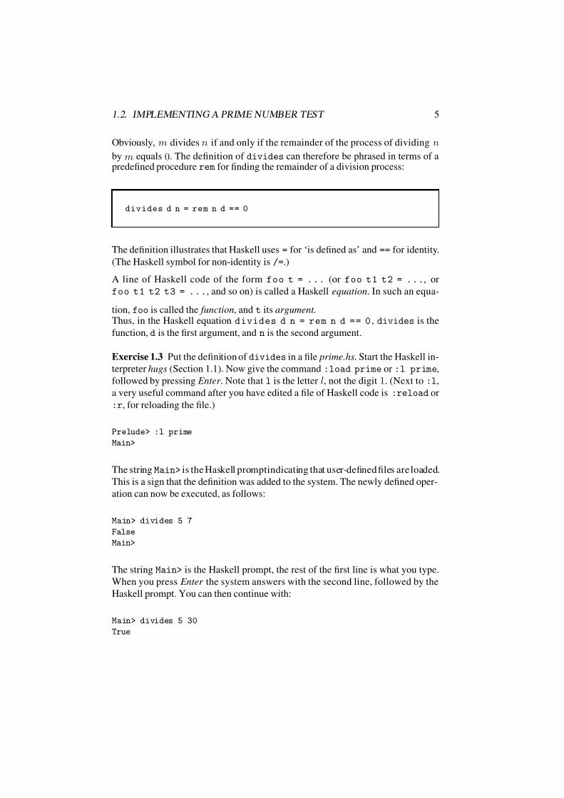
Obviously, m divides n if and only if the remainder of the process of dividing n
by m equals 0. The definition of divides can therefore be phrased in terms of apredefined procedure rem for finding the remainder of a division process:
divides d n = rem n d == 0
The definition illustrates that Haskell uses = for ‘is defined as’ and == for identity.
(The Haskell symbol for non-identity is /=.)
A line of Haskell code of the form foo t = ... (or foo t1 t2 = ..., or
foo t1 t2 t3 = ..., and so on) is called a Haskell equation. In such an equa-
tion, foo is called the function, and t its argument .Thus, in the Haskell equation divides d n = rem n d == 0 , divides is the
function, d is the first argument, and n is the second argument.
Exercise 1.3 Put the definition of divides in a file prime.hs. Start the Haskell in-
terpreter hugs (Section 1.1). Now give the command :load prime or :l prime,
followed by pressing Enter . Note that l is the letter l, not the digit 1. (Next to :l,
a very useful command after you have edited a file of Haskell code is :reload or
:r, for reloading the file.)
Prelude> :l prime
Main>
The string Main> is the Haskell promptindicating that user-defined files are loaded.
This is a sign that the definition was added to the system. The newly defined oper-
ation can now be executed, as follows:
Main> divides 5 7
False
Main>
The string Main> is the Haskell prompt, the rest of the first line is what you type.
When you press Enter the system answers with the second line, followed by the
Haskell prompt. You can then continue with:
Main> divides 5 30
True

7/16/2019 The Haskell Road to Logic Maths and Programming
http://slidepdf.com/reader/full/the-haskell-road-to-logic-maths-and-programming-5634fa29ef7e9 17/448
6 CHAPTER 1. GETTING STARTED
It is clear from the proposition above that all we have to do to implement a primal-
ity test is to give an implementation of the function LD. It is convenient to define
LD in terms of a second function LDF, for the least divisor starting from a given
threshold k, with k n. Thus, LDF(k)(n) is the least divisor of n that is k.
Clearly, LD(n) = LDF(2)(n). Now we can implement LD as follows:
l d n = l d f 2 n
This leaves the implementation ldf of LDF (details of the coding will be explainedbelow):
ldf k n | divides k n = k
| k^2 > n = n
| otherwise = ldf (k+1) n
The definition employs the Haskell operation ^ for exponentiation, > for ‘greater
than’, and + for addition.
The definition of ldf makes use of equation guarding. The first line of the ldf
definition handles the case where the first argument divides the second argument.
Every next line assumes that the previous lines do not apply. The second line
handles the case where the first argument does not divide the second argument,
and the square of the first argument is greater than the second argument. The third
line assumes that the first and second cases do not apply and handles all other
cases, i.e., the cases where k does not divide n and k2 < n.
The definition employs the Haskell condition operator | . A Haskell equation of the form
foo t | condition = ...
is called a guarded equation. We might have written the definition of ldf as a list
of guarded equations, as follows:
7/16/2019 The Haskell Road to Logic Maths and Programming
http://slidepdf.com/reader/full/the-haskell-road-to-logic-maths-and-programming-5634fa29ef7e9 18/448
1.2. IMPLEMENTING A PRIME NUMBER TEST 7
ldf k n | divides k n = kldf k n | k^2 > n = n
ldf k n = ldf (k+1) n
The expression condition, of type Bool (i.e., Boolean or truth value), is called
the guard of the equation.
A list of guarded equations such as
foo t | condition_1 = body_1
foo t | condition_2 = body_2
foo t | condition_3 = body_3
foo t = body_4
can be abbreviated as
foo t | condition_1 = body_1
| condition_2 = body_2
| condition_3 = body_3
| otherwise = body_4
Such a Haskell definition is read as follows:
• in case condition_1 holds, foo t is by definition equal to body_1,
• in case condition_1 does not hold but condition_2 holds, foo t is by
definition equal to body_2,
• in case condition_1 and condition_2 do not hold but condition_3
holds, foo t is by definition equal to body_3,
• and in case none of condition_1, condition_2 and condition_3 hold,
foo t is by definition equal to body_4.
When we are at the end of the list we know that none of the cases above in the list
apply. This is indicated by means of the Haskell reserved keyword otherwise.
Note that the procedure ldf is called again from the body of its own definition. We
will encounter such recursive procedure definitions again and again in the course
of this book (see in particular Chapter 7).

7/16/2019 The Haskell Road to Logic Maths and Programming
http://slidepdf.com/reader/full/the-haskell-road-to-logic-maths-and-programming-5634fa29ef7e9 19/448
8 CHAPTER 1. GETTING STARTED
Exercise 1.4 Suppose in the definition of ldf we replace the condition k^2 > n
by k^2 >= n, where >= expresses ‘greater than or equal’. Would that make anydifference to the meaning of the program? Why (not)?
Now we are ready for a definition of prime0, our first implementation of the test
for being a prime number.
prime0 n | n < 1 = error "not a positive integer"
| n == 1 = False
| otherwise = ld n == n
Haskell allows a call to the error operation in any definition. This is used to break
off operation and issue an appropriate message when the primality test is used fornumbers below 1. Note that error has a parameter of type String (indicated by
the double quotes).
The definition employs the Haskell operation < for ‘less than’.
Intuitively, what the definition prime0 says is this:
1. the primality test should not be applied to numbers below 1,
2. if the test is applied to the number 1 it yields ‘false’,
3. if it is applied to an integer n greater than 1 it boils down to checking that
LD(n) = n. In view of the proposition we proved above, this is indeed a
correct primality test.
Exercise 1.5 Add these definitions to the file prime.hs and try them out.
Remark. The use of variables in functional programming has much in common
with the use of variables in logic. The definition divides d n = rem n d == 0
is equivalent to divides x y = rem y x == 0 . This is because the variables
denote arbitrary elements of the type over which they range. They behave like
universally quantified variables, and just as in logic the definition does not depend
on the variable names.
1.3 Haskell Type Declarations
Haskell has a concise way to indicate that divides consumes an integer, then
another integer, and produces a truth value (called Bool in Haskell). Integers and

7/16/2019 The Haskell Road to Logic Maths and Programming
http://slidepdf.com/reader/full/the-haskell-road-to-logic-maths-and-programming-5634fa29ef7e9 20/448
1.3. HASKELL TYPE DECLARATIONS 9
truth values are examples of types. See Section 2.1 for more on the type Bool.
Section 1.6 gives more information about types in general. Arbitrary precisionintegers in Haskell have type Integer. The following line gives a so-called type
declaration for the divides function.
divides :: Integer -> Integer -> Bool
Integer -> Integer -> Bool is short for Integer -> (Integer -> Bool).
A type of the form a - > b classifies a procedure that takes an argument of type a
to produce a result of type b. Thus, divides takes an argument of type Integer
and produces a result of type Integer -> Bool, i.e., a procedure that takes an
argument of type Integer, and produces a result of type Bool.
The full code for divides, including the type declaration, looks like this:
divides :: Integer -> Integer -> Bool
divides d n = rem n d == 0
If d is an expression of type Integer, then divides d is an expression of type
Integer -> Bool. The shorthand that we will use for
d is an expression of type Integer
is: d :: Integer.
Exercise 1.6 Can you gather from the definition of divides what the type decla-
ration for rem would look like?
Exercise 1.7 The hugs system has a command for checking the types of expres-sions. Can you explain the following (please try it out; make sure that the filewith the definition of divides is loaded, together with the type declaration fordivides):
Main> :t divides 5
divides 5 :: Integer -> Bool
Main> :t divides 5 7divides 5 7 :: Bool
Main>

7/16/2019 The Haskell Road to Logic Maths and Programming
http://slidepdf.com/reader/full/the-haskell-road-to-logic-maths-and-programming-5634fa29ef7e9 21/448
10 CHAPTER 1. GETTING STARTED
The expression divides 5 :: Integer -> Bool is called a type judgment .
Type judgments in Haskell have the form expression :: type.
In Haskell it is not strictly necessary to give explicit type declarations. For in-
stance, the definition of divides works quite well without the type declaration,
since the system can infer the type from the definition. However, it is good pro-
gramming practice to give explicit type declarations even when this is not strictly
necessary. These type declarations are an aid to understanding, and they greatly
improve the digestibility of functional programs for human readers. A further
advantage of the explicit type declarations is that they facilitate detection of pro-
gramming mistakes on the basis of type errors generated by the interpreter. You
will find that many programming errors already come to light when your programgets loaded. The fact that your program is well typed does not entail that it is
correct, of course, but many incorrect programs do have typing mistakes.
The full code for ld, including the type declaration, looks like this:
ld :: Integer -> Integer
l d n = l d f 2 n
The full code for ldf, including the type declaration, looks like this:
ldf :: Integer -> Integer -> Integer
ldf k n | divides k n = k
| k^2 > n = n
| otherwise = ldf (k+1) n
The first line of the code states that the operation ldf takes two integers and pro-
duces an integer.
The full code for prime0, including the type declaration, runs like this:

7/16/2019 The Haskell Road to Logic Maths and Programming
http://slidepdf.com/reader/full/the-haskell-road-to-logic-maths-and-programming-5634fa29ef7e9 22/448
1.4. IDENTIFIERS IN HASKELL 11
prime0 :: Integer -> Boolprime0 n | n < 1 = error "not a positive integer"
| n == 1 = False
| otherwise = ld n == n
The first line of the code declares that the operation prime0 takes an integer and
produces (or returns, as programmers like to say) a Boolean (truth value).
In programming generally, it is useful to keep close track of the nature of the
objects that are being represented. This is because representationshave to be stored
in computer memory, and one has to know how much space to allocate for this
storage. Still, there is no need to always specify the nature of each data-type
explicitly. It turns out that much information about the nature of an object can be
inferred from how the object is handled in a particular program, or in other words,
from the operations that are performed on that object.
Take again the definition of divides. It is clear from the definition that an oper-ation is defined with two arguments, both of which are of a type for which rem isdefined, and with a result of type Bool (for r e m n d = = 0 is a statement that canturn out true or false). If we check the type of the built-in procedure rem we get:
Prelude> :t rem
rem :: Integral a => a -> a -> a
In this particular case, the type judgment gives a type scheme rather than a type. It
means: if a is a type of class Integral, then rem is of type a - > a - > a. Here
a is used as a variable ranging over types.
In Haskell, Integral is the class (see Section 4.2) consisting of the two types for
integer numbers, Int and Integer. The difference between Int and Integer
is that objects of type Int have fixed precision, objects of type Integer have
arbitrary precision.
The type of divides can now be inferred from the definition. This is what we getwhen we load the definition of divides without the type declaration:
Main> :t divides
divides :: Integral a => a -> a -> Bool
1.4 Identifiers in Haskell
In Haskell, there are two kinds of identifiers:

7/16/2019 The Haskell Road to Logic Maths and Programming
http://slidepdf.com/reader/full/the-haskell-road-to-logic-maths-and-programming-5634fa29ef7e9 23/448
12 CHAPTER 1. GETTING STARTED
•Variable identifiers are used to name functions. They have to start with a
lower-case letter. E.g., map, max, fct2list, fctToList, fct_to_list.
• Constructor identifiers are used to name types. They have to start with an
upper-case letter. Examples are True, False.
Functions are operations on data-structures, constructors are the building blocks
of the data structures themselves (trees, lists, Booleans, and so on).
Names of functions always start with lower-case letters, and may contain both
upper- and lower-case letters, but also digits, underscores and the prime symbol
’. The following reserved keywords have special meanings and cannot be used to
name functions.
case class data default deriving do else
if import in infix infixl infixr instance
let module newtype of then type where
The use of these keywords will be explained as we encounter them. at the begin-
ning of a word is treated as a lower-case character. The underscore character all
by itself is a reserved word for the wild card pattern that matches anything (page
141).
There is one more reserved keyword that is particular to Hugs: forall, for the defi-
nition of functions that take polymorphic arguments. See the Hugs documentation
for further particulars.
1.5 Playing the Haskell Game
This section consists of a number of further examples and exercises to get you
acquainted with the programming language of this book. To save you the trouble
of keying in the programs below, you should retrieve the module GS.hs for the
present chapter from the book website and load it in hugs. This will give you a
system prompt GS>, indicating that all the programs from this chapter are loaded.
In the next example, we use Int for the type of fixed precision integers, and [Int]
for lists of fixed precision integers.
Example 1.8 Here is a function that gives the minimum of a list of integers:
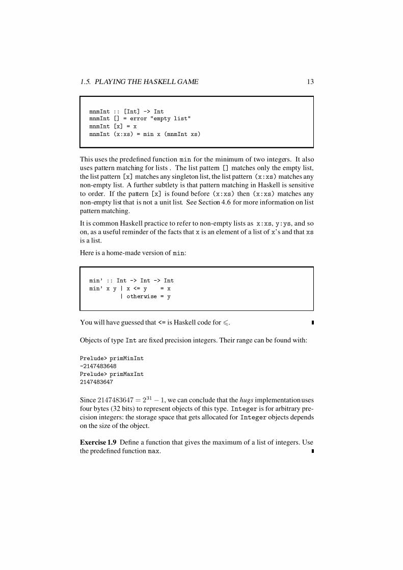
7/16/2019 The Haskell Road to Logic Maths and Programming
http://slidepdf.com/reader/full/the-haskell-road-to-logic-maths-and-programming-5634fa29ef7e9 24/448
1.5. PLAYING THE HASKELL GAME 13
mnmInt :: [Int] -> Int mnmInt [] = error "empty list"
mnmInt [x] = x
mnmInt (x:xs) = min x (mnmInt xs)
This uses the predefined function min for the minimum of two integers. It also
uses pattern matching for lists . The list pattern [] matches only the empty list,
the list pattern [x] matches any singleton list, the list pattern (x:xs) matches any
non-empty list. A further subtlety is that pattern matching in Haskell is sensitive
to order. If the pattern [x] is found before (x:xs) then (x:xs) matches any
non-empty list that is not a unit list. See Section 4.6 for more information on list
pattern matching.
It is common Haskell practice to refer to non-empty lists as x:xs, y:ys, and so
on, as a useful reminder of the facts that x is an element of a list of x’s and that xs
is a list.
Here is a home-made version of min:
min’ :: Int -> Int -> Int
min’ x y | x <= y = x
| otherwise = y
You will have guessed that <= is Haskell code for .
Objects of type Int are fixed precision integers. Their range can be found with:
Prelude> primMinInt
-2147483648
Prelude> primMaxInt
2147483647
Since 2147483647 = 231 − 1, we can conclude that the hugs implementation uses
four bytes (32 bits) to represent objects of this type. Integer is for arbitrary pre-
cision integers: the storage space that gets allocated for Integer objects depends
on the size of the object.
Exercise 1.9 Define a function that gives the maximum of a list of integers. Use
the predefined function max.

7/16/2019 The Haskell Road to Logic Maths and Programming
http://slidepdf.com/reader/full/the-haskell-road-to-logic-maths-and-programming-5634fa29ef7e9 25/448
14 CHAPTER 1. GETTING STARTED
Conversion from Prefix to Infix in Haskell A function can be converted to an
infix operator by putting its name in back quotes, like this:
Prelude> max 4 5
5
Prelude> 4 ‘max‘ 5
5
Conversely, an infix operator is converted to prefix by putting the operator in round
brackets (p. 21).
Exercise 1.10 Define a function removeFst that removes the first occurrence of
an integer m from a list of integers. If m does not occur in the list, the list remains
unchanged.
Example 1.11 We define a function that sorts a list of integers in order of increas-
ing size, by means of the following algorithm:
• an empty list is already sorted.
• if a list is non-empty, we put its minimum in front of the result of sorting the
list that results from removing its minimum.
This is implemented as follows:
srtInts :: [Int] -> [Int]srtInts [] = []
srtInts xs = m : (srtInts (removeFst m xs)) where m = mnmInt xs
Here removeFst is the function you defined in Exercise 1.10. Note that the second
clause is invoked when the first one does not apply, i.e., when the argument of
srtInts is not empty. This ensures that mnmInt xs never gives rise to an error.
Note the use of a where construction for the local definition of an auxiliary func-
tion.
Remark. Haskell has two ways to locally define auxiliary functions, where and
let constructions. The where construction is illustrated in Example 1.11. This
can also expressed with let, as follows:

7/16/2019 The Haskell Road to Logic Maths and Programming
http://slidepdf.com/reader/full/the-haskell-road-to-logic-maths-and-programming-5634fa29ef7e9 26/448
1.5. PLAYING THE HASKELL GAME 15
srtInts’ :: [Int] -> [Int]srtInts’ [] = []
srtInts’ xs = let
m = mnmInt xs
in m : (srtInts’ (removeFst m xs))
The let construction uses the reserved keywords let and in.
Example 1.12 Here is a function that calculates the average of a list of integers.
The average of m and n is given bym+n
2 , the average of a list of k integersn1, . . . , nk is given by n1+···+nk
k . In general, averages are fractions, so the result
type of average should not be Int but the Haskell data-type for floating point
numbers, which is Float. There are predefined functions sum for the sum of a list
of integers, and length for the length of a list. The Haskell operation for division
/ expects arguments of type Float (or more precisely, of Fractional type, and
Float is such a type), so we need a conversion function for converting Ints into
Floats. This is done by fromInt. The function average can now be written as:
average :: [Int] -> Float
average [] = error "empty list"
average xs = fromInt (sum xs) / fromInt (length xs)
Again, it is instructive to write our own homemade versions of sum and length.
Here they are:
sum’ :: [Int] -> Int
sum’ [] = 0sum’ (x:xs) = x + sum’ xs

7/16/2019 The Haskell Road to Logic Maths and Programming
http://slidepdf.com/reader/full/the-haskell-road-to-logic-maths-and-programming-5634fa29ef7e9 27/448
16 CHAPTER 1. GETTING STARTED
length’ :: [a] -> Intlength’ [] = 0
length’ (x:xs) = 1 + length’ xs
Note that the type declaration for length’ contains a variable a. This variable
ranges over all types, so [a] is the type of a list of objects of an arbitrary type a.
We say that [a] is a type scheme rather than a type. This way, we can use the same
function length’ for computing the length of a list of integers, the length of a list
of characters, the length of a list of strings (lists of characters), and so on.
The type [Char] is abbreviated as String. Examples of characters are ’a’, ’b’
(note the single quotes) examples of strings are "Russell" and "Cantor" (note
the double quotes). In fact, "Russell" can be seen as an abbreviation of the list
[’R’,’u’,’s’,’s’,’e’,’l’,’l’].
Exercise 1.13 Write a function count for counting the number of occurrences of
a character in a string. In Haskell, a character is an object of type Char, and a string
an object of type String, so the type declaration should run: count :: Char ->
String -> Int.
Exercise 1.14 A function for transforming strings into strings is of type String
-> String. Write a function blowup that converts a string
a1a2a3 · · ·to
a1a2a2a3a3a3 · · · .
blowup "bang!" should yield "baannngggg!!!!!". (Hint: use ++ for string
concatenation.)
Exercise 1.15 Write a function srtString :: [String] -> [String] that
sorts a list of strings in alphabetical order.
Example 1.16 Suppose we want to check whether a string str1 is a prefix of
a string str2. Then the answer to the question prefix str1 str2 should be
either yes (true) or no (false), i.e., the type declaration for prefix should run:
prefix :: String -> String -> Bool.
Prefixes of a string ys are defined as follows:

7/16/2019 The Haskell Road to Logic Maths and Programming
http://slidepdf.com/reader/full/the-haskell-road-to-logic-maths-and-programming-5634fa29ef7e9 28/448
1.6. HASKELL TYPES 17
1. [] is a prefix of ys,
2. if xs is a prefix of ys, then x:xs is a prefix of x:ys,
3. nothing else is a prefix of ys.
Here is the code for prefix that implements this definition:
prefix :: String -> String -> Bool
prefix [] ys = True
prefix (x:xs) [] = False
prefix (x:xs) (y:ys) = (x==y) && prefix xs ys
The definition of prefix uses the Haskell operator && for conjunction.
Exercise 1.17 Write a function substring :: String -> String -> Bool
that checks whether str1 is a substring of str2.
The substrings of an arbitrary string ys are given by:
1. if xs is a prefix of ys, xs is a substring of ys,
2. if ys equals y:ys’ and xs is a substring of ys’, xs is a substring of ys,
3. nothing else is a substring of ys.
1.6 Haskell Types
The basic Haskell types are:
• Int and Integer, to represent integers. Elements of Integer are un-
bounded. That’s why we used this type in the implementation of the prime
number test.
• Float and Double represent floating point numbers. The elements of Double
have higher precision.
• Bool is the type of Booleans.

7/16/2019 The Haskell Road to Logic Maths and Programming
http://slidepdf.com/reader/full/the-haskell-road-to-logic-maths-and-programming-5634fa29ef7e9 29/448
18 CHAPTER 1. GETTING STARTED
•Char is the type of characters.
Note that the name of a type always starts with a capital letter.
To denote arbitrary types, Haskell allows the use of type variables. For these, a, b,
..., are used.
New types can be formed in several ways:
• By list-formation: if a is a type, [a] is the type of lists over a. Examples:
[Int] is the type of lists of integers; [Char] is the type of lists of characters,
or strings.
• By pair- or tuple-formation: if a and b are types, then (a,b) is the type
of pairs with an object of type a as their first component, and an object of
type b as their second component. Similarly, triples, quadruples, . . . , can be
formed. If a, b and c are types, then (a,b,c) is the type of triples with an
object of type a as their first component, an object of type b as their second
component, and an object of type c as their third component. And so on
(p. 139).
• By function definition: a - > b is the type of a function that takes arguments
of type a and returns values of type b.
• By defining your own data-type from scratch, with a data type declaration.
More about this in due course.
Pairs will be further discussed in Section 4.5, lists and list operations in Section
4.6.
Operations are procedures for constructing objects of a certain types b from ingre-
dients of a type a. Now such a procedure can itself be given a type: the type of
a transformer from a type objects to b type objects. The type of such a procedure
can be declared in Haskell as a - > b.
If a function takes two string arguments and returns a string then this can be
viewed as a two-stage process: the function takes a first string and returns a
transformer from strings to strings. It then follows that the type is String ->
(String -> String), which can be written as String -> String -> String,
because of the Haskell convention that -> associates to the right.
Exercise 1.18 Find expressions with the following types:
1. [String]

7/16/2019 The Haskell Road to Logic Maths and Programming
http://slidepdf.com/reader/full/the-haskell-road-to-logic-maths-and-programming-5634fa29ef7e9 30/448
1.7. THE PRIME FACTORIZATION ALGORITHM 19
2. (Bool,String)
3. [(Bool,String)]
4. ([Bool],String)
5. Bool -> Bool
Test your answers by means of the Hugs command :t.
Exercise 1.19 Use the Hugs command :t to find the types of the following pre-
defined functions:
1. head
2. last
3. init
4. fst
5. (++)
6. flip
7. flip (++)
Next, supply these functions with arguments of the expected types, and try to guess
what these functions do.
1.7 The Prime Factorization Algorithm
Let n be an arbitrary natural number > 1. A prime factorization of n is a list of
prime numbers p1, . . . , pj with the property that p1 · · · · · pj = n. We will show
that a prime factorization of every natural number n > 1 exists by producing one
by means of the following method of splitting off prime factors:
WHILE n = 1 DO BEGIN p := LD(n); n :=n
pEND
Here := denotes assignment or the act of giving a variable a new value. As we
have seen, LD(n) exists for every n with n > 1. Moreover, we have seen that
LD(n) is always prime. Finally, it is clear that the procedure terminates, for every
round through the loop will decrease the size of n.
7/16/2019 The Haskell Road to Logic Maths and Programming
http://slidepdf.com/reader/full/the-haskell-road-to-logic-maths-and-programming-5634fa29ef7e9 31/448
20 CHAPTER 1. GETTING STARTED
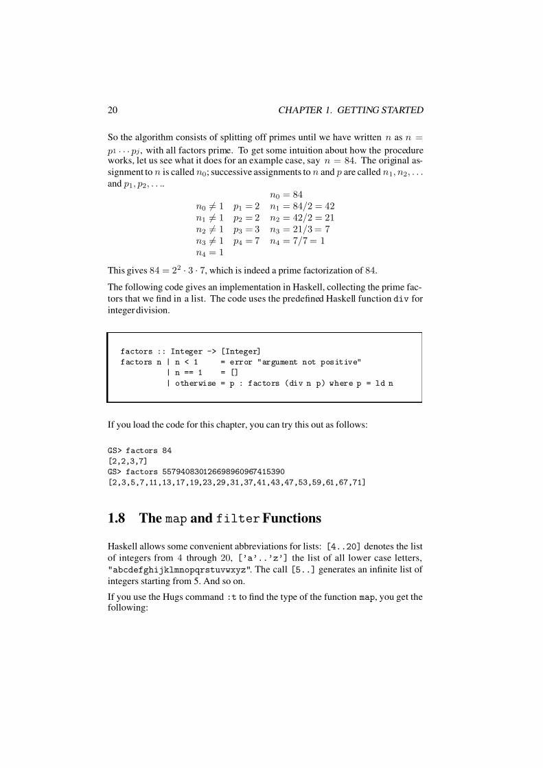
So the algorithm consists of splitting off primes until we have written n as n =
p1 · · · pj, with all factors prime. To get some intuition about how the procedureworks, let us see what it does for an example case, say n = 84. The original as-
signment to n is called n0; successive assignments to n and p are called n1, n2, . . .and p1, p2, . . ..
n0 = 84n0 = 1 p1 = 2 n1 = 84/2 = 42n1 = 1 p2 = 2 n2 = 42/2 = 21n2 = 1 p3 = 3 n3 = 21/3 = 7n3 = 1 p4 = 7 n4 = 7/7 = 1n4 = 1
This gives 84 = 22 · 3 · 7, which is indeed a prime factorization of 84.
The following code gives an implementation in Haskell, collecting the prime fac-
tors that we find in a list. The code uses the predefined Haskell function div for
integer division.
factors :: Integer -> [Integer]
factors n | n < 1 = error "argument not positive"
| n == 1 = []
| otherwise = p : factors (div n p) where p = ld n
If you load the code for this chapter, you can try this out as follows:
GS> factors 84
[2,2,3,7]
GS> factors 557940830126698960967415390
[2,3,5,7,11,13,17,19,23,29,31,37,41,43,47,53,59,61,67,71]
1.8 The map and filterFunctions
Haskell allows some convenient abbreviations for lists: [4..20] denotes the list
of integers from 4 through 20, [’a’..’z’] the list of all lower case letters,
"abcdefghijklmnopqrstuvwxyz". The call [5..] generates an infinite list of
integers starting from 5. And so on.
If you use the Hugs command :t to find the type of the function map, you get thefollowing:

7/16/2019 The Haskell Road to Logic Maths and Programming
http://slidepdf.com/reader/full/the-haskell-road-to-logic-maths-and-programming-5634fa29ef7e9 32/448
1.8. THE MAP AND FILTER FUNCTIONS 21
Prelude> :t map
map :: (a -> b) -> [a] -> [b]
The function map takes a function and a list and returns a list containing the results
of applying the function to the individual list members.
If f is a function of type a - > b and xs is a list of type [a], then map f xs willreturn a list of type [b]. E.g., map (^2) [1..9] will produce the list of squares
[1, 4, 9, 16, 25, 36, 49, 64, 81]
You should verify this by trying it out in Hugs. The use of (^2) for the operation
of squaring demonstrates a new feature of Haskell, the construction of sections.
Conversion from Infix to Prefix, Construction of Sections If op is an infix
operator, (op) is the prefix version of the operator. Thus, 2^10 can also be written
as (^) 2 10. This is a special case of the use of sections in Haskell.
In general, if op is an infix operator, (op x) is the operation resulting from ap-
plying op to its right hand side argument, (x op) is the operation resulting from
applying op to its left hand side argument, and (op) is the prefix version of the
operator (this is like the abstraction of the operator from both arguments).
Thus (^2) is the squaring operation, (2^) is the operation that computes powers
of 2, and (^) is exponentiation. Similarly, (>3) denotes the property of being
greater than 3, (3>) the property of being smaller than 3, and (>) is the prefix
version of the ‘greater than’ relation.
The call map (2^) [1..10] will yield
[2, 4, 8, 16, 32, 64, 128, 256, 512, 1024]
If p is a property (an operation of type a -> Bool) and xs is a list of type [a],then map p xs will produce a list of type Bool (a list of truth values), like this:
Prelude> map (>3) [1..9]
[False, False, False, True, True, True, True, True, True]
Prelude>
The function map is predefined in Haskell, but it is instructive to give our own
version:

7/16/2019 The Haskell Road to Logic Maths and Programming
http://slidepdf.com/reader/full/the-haskell-road-to-logic-maths-and-programming-5634fa29ef7e9 33/448
22 CHAPTER 1. GETTING STARTED
map :: (a -> b) -> [a] -> [b] map f [] = []
map f (x:xs) = (f x) : (map f xs)
Note that if you try to load this code, you will get an error message:
Definition of variable "map" clashes with import.
The error message indicates that the function name map is already part of the name
space for functions, and is not available anymore for naming a function of your
own making.
Exercise 1.20 Use map to write a function lengths that takes a list of lists and
returns a list of the corresponding list lengths.
Exercise 1.21 Use map to write a function sumLengths that takes a list of lists
and returns the sum of their lengths.
Another useful function is filter, for filtering out the elements from a list that
satisfy a given property. This is predefined, but here is a home-made version:
filter :: (a -> Bool) -> [a] -> [a]
filter p [] = []
filter p (x:xs) | p x = x : filter p xs
| otherwise = filter p xs
Here is an example of its use:
GS> filter (>3) [1..10]
[4,5,6,7,8,9,10]
Example 1.22 Here is a program primes0 that filters the prime numbers from the
infinite list [2..] of natural numbers:

7/16/2019 The Haskell Road to Logic Maths and Programming
http://slidepdf.com/reader/full/the-haskell-road-to-logic-maths-and-programming-5634fa29ef7e9 34/448
1.8. THE MAP AND FILTER FUNCTIONS 23
primes0 :: [Integer]primes0 = filter prime0 [2..]
This produces an infinite list of primes. (Why infinite? See Theorem 3.33.) The
list can be interrupted with ‘Control-C’.
Example 1.23 Given that we can produce a list of primes, it should be possible
now to improve our implementation of the function LD. The function ldf used in
the definition of ld looks for a prime divisor of n by checking k|n for all k with
2 k √
n. In fact, it is enough to check p|n for the primes p with 2 p √
n.
Here are functions ldp and ldpf that perform this more efficient check:
ldp :: Integer -> Integer
ldp n = ldpf primes1 n
ldpf :: [Integer] -> Integer -> Integer
ldpf (p:ps) n | rem n p == 0 = p| p^2 > n = n
| otherwise = ldpf ps n
ldp makes a call to primes1, the list of prime numbers. This is a first illustration
of a ‘lazy list’. The list is called ‘lazy’ because we compute only the part of the
list that we need for further processing. To define primes1 we need a test for
primality, but that test is itself defined in terms of the function LD, which in turn
refers to primes1. We seem to be running around in a circle. This circle can be
made non-vicious by avoiding the primality test for 2. If it is given that 2 is prime,
then we can use the primality of 2 in the LD check that 3 is prime, and so on, and
we are up and running.

7/16/2019 The Haskell Road to Logic Maths and Programming
http://slidepdf.com/reader/full/the-haskell-road-to-logic-maths-and-programming-5634fa29ef7e9 35/448
24 CHAPTER 1. GETTING STARTED
primes1 :: [Integer]primes1 = 2 : filter prime [3..]
prime :: Integer -> Bool
prime n | n < 1 = error "not a positive integer"
| n == 1 = False
| otherwise = ldp n == n
Replacing the definition of primes1 by filter prime [2..] creates vicious
circularity, with stack overflow as a result (try it out). By running the program
primes1 against primes0 it is easy to check that primes1 is much faster.
Exercise 1.24 What happens when you modify the defining equation of ldp as
follows:
ldp :: Integer -> Integer
ldp = ldpf primes1
Can you explain?
1.9 Haskell Equations and Equational ReasoningThe Haskell equations f x y = . . . used in the definition of a function f are
genuine mathematical equations. They state that the left hand side and the right
hand side of the equation have the same value. This is very different from the use
of = in imperative languages like C or Java. In a C or Java program, the statement
x = x*y does not mean that x and x ∗ y have the same value, but rather it is a
command to throw away the old value of x and put the value of x ∗ y in its place.
It is a so-called destructive assignment statement : the old value of a variable is
destroyed and replaced by a new one.
Reasoning about Haskell definitions is a lot easier than reasoning about programs
that use destructive assignment. In Haskell, standard reasoning about mathemat-
ical equations applies. E.g., after the Haskell declarations x = 1 and y = 2, the
Haskell declaration x = x + y will raise an error "x" multiply defined. Be-
cause = in Haskell has the meaning “is by definition equal to”, while redefinition

7/16/2019 The Haskell Road to Logic Maths and Programming
http://slidepdf.com/reader/full/the-haskell-road-to-logic-maths-and-programming-5634fa29ef7e9 36/448
1.9. HASKELL EQUATIONS AND EQUATIONAL REASONING 25
is forbidden, reasoning about Haskell functions is standard equational reasoning.
Let’s try this out on a simple example.
a = 3
b = 4
f :: Integer -> Integer -> Integer
f x y = x^2 + y^2
To evaluate f a ( f a b ) by equational reasoning, we can proceed as follows:
f a (f a b) = f a (a2 + b2)
= f 3 (32
+ 42
)= f 3 (9 + 16)
= f 3 25
= 32 + 252
= 9 + 625
= 634
The rewriting steps use standard mathematical laws and the Haskell definitions of
a, b, f . And, in fact, when running the program we get the same outcome:
GS> f a (f a b)
634
GS>
Remark. We already encountered definitions where the function that is being
defined occurs on the right hand side of an equation in the definition. Here is
another example:
g :: Integer -> Integer
g 0 = 0
g (x+1) = 2 * (g x)
Not everything that is allowed by the Haskell syntax makes semantic sense, how-
ever. The following definitions, although syntactically correct, do not properly
define functions:

7/16/2019 The Haskell Road to Logic Maths and Programming
http://slidepdf.com/reader/full/the-haskell-road-to-logic-maths-and-programming-5634fa29ef7e9 37/448
26 CHAPTER 1. GETTING STARTED
h1 :: Integer -> Integerh 1 0 = 0
h1 x = 2 * (h1 x)
h2 :: Integer -> Integer
h 2 0 = 0
h2 x = h2 (x+1)
The problem is that for values other than 0 the definitions do not give recipes for
computing a value. This matter will be taken up in Chapter 7.
1.10 Further Reading
The standard Haskell operations are defined in the file Prelude.hs, which you
should be able to locate somewhere on any system that runs hugs. Typically, the
file resides in /usr/lib/hugs/libraries/Hugs/.
In case Exercise 1.19 has made you curious, the definitions of these example func-
tions can all be found in Prelude.hs. If you want to quickly learn a lot about how to
program in Haskell, you should get into the habit of consulting this file regularly.
The definitions of all the standard operations are open source code, and are there
for you to learn from. The Haskell Prelude may be a bit difficult to read at first,
but you will soon get used to the syntax and acquire a taste for the style.
Various tutorials on Haskell and Hugs can be found on the Internet: see e.g.[HFP96] and [JR+]. The definitive reference for the language is [Jon03]. A text-
book on Haskell focusing on multimedia applications is [Hud00]. Other excellent
textbooks on functional programming with Haskell are [Tho99] and, at a more ad-
vanced level, [Bir98]. A book on discrete mathematics that also uses Haskell as a
tool, and with a nice treatment of automated proof checking, is [HO00].
7/16/2019 The Haskell Road to Logic Maths and Programming
http://slidepdf.com/reader/full/the-haskell-road-to-logic-maths-and-programming-5634fa29ef7e9 38/448
Chapter 2
Talking about Mathematical
Objects
Preview
To talk about mathematical objects with ease it is useful to introduce some sym-
bolic abbreviations. These symbolic conventions are meant to better reveal the
structure of our mathematical statements. This chapter concentrates on a few (infact: seven), simple words or phrases that are essential to the mathematical vo-
cabulary: not , if , and , or , if and only if , for all and for some. We will introduce
symbolic shorthands for these words, and we look in detail at how these building
blocks are used to construct the logical patterns of sentences. After having isolated
the logical key ingredients of the mathematical vernacular, we can systematically
relate definitions in terms of these logical ingredients to implementations, thus
building a bridge between logic and computer science.
The use of symbolic abbreviations in specifying algorithms makes it easier to take
the step from definitions to the procedures that implement those definitions. In a
similar way, the use of symbolic abbreviations in making mathematical statements
makes it easier to construct proofs of those statements. Chances are that you are
more at ease with programming than with proving things. However that may be,
in the chapters to follow you will get the opportunity to improve your skills in both
of these activities and to find out more about the way in which they are related.
27

7/16/2019 The Haskell Road to Logic Maths and Programming
http://slidepdf.com/reader/full/the-haskell-road-to-logic-maths-and-programming-5634fa29ef7e9 39/448
28 CHAPTER 2. TALKING ABOUT MATHEMATICAL OBJECTS
module TAMO
where
2.1 Logical Connectives and their Meanings
Goal To understand how the meanings of statements using connectives can be
described by explaining how the truth (or falsity) of the statement depends on
the truth (or falsity) of the smallest parts of this statement. This understanding
leads directly to an implementation of the logical connectives as truth functionalprocedures.
In ordinary life, there are many statements that do not have a definite truth value,
for example ‘Barnett Newman’s Who is Afraid of Red, Yellow and Blue III is a
beautiful work of art,’ or ‘Daniel Goldreyer’s restoration of Who is Afraid of Red,
Yellow and Blue III meets the highest standards.’
Fortunately the world of mathematics differs from the Amsterdam Stedelijk Mu-
seum of Modern Art in the following respect. In the world of mathematics, things
are so much clearer that many mathematicians adhere to the following slogan:
every statement that makes mathematical sense is either true or false.
The idea behind this is that (according to the adherents) the world of mathematics
exists independently of the mind of the mathematician. Doing mathematics is the
activity of exploring this world. In proving new theorems one discovers new facts
about the world of mathematics, in solving exercises one rediscovers known facts
for oneself. (Solving problems in a mathematics textbook is like visiting famous
places with a tourist guide.)
This belief in an independent world of mathematical fact is called Platonism, after
the Greek philosopher Plato, who even claimed that our everyday physical world
is somehow an image of this ideal mathematical world. A mathematical Platonist
holds that every statement that makes mathematical sense has exactly one of the
two truth values. Of course, a Platonist would concede that we may not know
which value a statement has, for mathematics has numerous open problems. Still,
a Platonist would say that the true answer to an open problem in mathematics like
‘Are there infinitely many Mersenne primes?’ (Example 3.40 from Chapter 3) is
7/16/2019 The Haskell Road to Logic Maths and Programming
http://slidepdf.com/reader/full/the-haskell-road-to-logic-maths-and-programming-5634fa29ef7e9 40/448
2.1. LOGICAL CONNECTIVES AND THEIR MEANINGS 29
either ‘yes’ or ‘no’. The Platonists would immediately concede that nobody may
know the true answer, but that, they would say, is an altogether different matter.
Of course, matters are not quite this clear-cut, but the situation is certainly a lot
better than in the Amsterdam Stedelijk Museum. In the first place, it may not
be immediately obvious which statements make mathematical sense (see Example
4.5). In the second place, you don’t have to be a Platonist to do mathematics. Not
every working mathematician agrees with the statement that the world of mathe-
matics exists independently of the mind of the mathematical discoverer. The Dutch
mathematician Brouwer (1881–1966) and his followers have argued instead that
the mathematical reality has no independent existence, but is created by the work-
ing mathematician. According to Brouwer the foundation of mathematics is in the
intuition of the mathematical intellect. A mathematical Intuitionist will therefore
not accept certain proof rules of classical mathematics, such as proof by contra-
diction (see Section 3.3), as this relies squarely on Platonist assumptions.
Although we have no wish to pick a quarrel with the intuitionists, in this book we
will accept proof by contradiction, and we will in general adhere to the practice of
classical mathematics and thus to the Platonist creed.
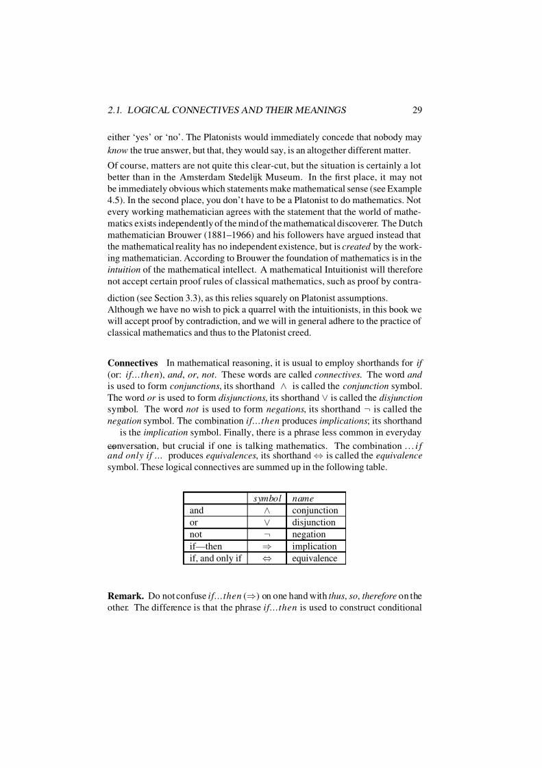
Connectives In mathematical reasoning, it is usual to employ shorthands for if
(or: if...then), and , or , not . These words are called connectives. The word and
is used to form conjunctions, its shorthand ∧ is called the conjunction symbol.
The word or is used to form disjunctions, its shorthand ∨ is called the disjunction
symbol. The word not is used to form negations, its shorthand ¬ is called the
negation symbol. The combination if...then produces implications; its shorthand
⇒is the implication symbol. Finally, there is a phrase less common in everyday
conversation, but crucial if one is talking mathematics. The combination . . . i f and only if ... produces equivalences, its shorthand ⇔ is called the equivalence
symbol. These logical connectives are summed up in the following table.
symbol name
and ∧ conjunction
or ∨ disjunction
not ¬ negation
if—then ⇒ implication
if, and only if ⇔ equivalence
Remark. Do not confuse if...then (⇒) on one hand with thus, so, therefore on the
other. The difference is that the phrase if...then is used to construct conditional

7/16/2019 The Haskell Road to Logic Maths and Programming
http://slidepdf.com/reader/full/the-haskell-road-to-logic-maths-and-programming-5634fa29ef7e9 41/448
30 CHAPTER 2. TALKING ABOUT MATHEMATICAL OBJECTS
statements, while thus (therefore, so) is used to combine statements into pieces of
mathematical reasoning (or: mathematical proofs). We will never write ⇒ whenwe want to conclude from one mathematical statement to the next. The rules of
inference, the notion of mathematical proof, and the proper use of the word thus
are the subject of Chapter 3.
Iff. In mathematical English it is usual to abbreviate if, and only if to iff . We will
also use ⇔ as a symbolic abbreviation. Sometimes the phrase just in case is used
with the same meaning.
The following describes, for every connective separately, how the truth value of
a compound using the connective is determined by the truth values of its compo-
nents. For most connectives, this is rather obvious. The cases for ⇒ and ∨ have
some peculiar difficulties.The letters P and Q are used for arbitrary statements. We use t for ‘true’, and f for
‘false’. The set t, f is the set of truth values.
Haskell uses True and False for the truth values. Together, these form the type
Bool. This type is predefined in Haskell as follows:
data Bool = False | True
Negation
An expression of the form ¬P (not P , it is not the case that P , etc.) is called the
negation of P . It is true (has truth value t) just in case P is false (has truth value
f ).
In an extremely simple table, this looks as follows:
P ¬P t f
f t
This table is called the truth table of the negation symbol.
The implementation of the standard Haskell function not reflects this truth table:

7/16/2019 The Haskell Road to Logic Maths and Programming
http://slidepdf.com/reader/full/the-haskell-road-to-logic-maths-and-programming-5634fa29ef7e9 42/448
2.1. LOGICAL CONNECTIVES AND THEIR MEANINGS 31
not :: Bool -> Boolnot True = False
not False = True
This definition is part of Prelude.hs, the file that contains the predefined Haskell
functions.
Conjunction
The expression P ∧ Q ((both) P and Q) is called the conjunction of P and Q. P and Q are called conjuncts of P ∧ Q. The conjunction P ∧ Q is true iff P and
Q are both true.
Truth table of the conjunction symbol:
P Q P ∧ Qt t t
t f f
f t f
f f f
This is reflected in definition of the Haskell function for conjunction, && (also from
Prelude.hs):
(&&) :: Bool -> Bool -> Bool
False && x = False
True && x = x
What this says is: if the first argument of a conjunction evaluates to false, then
the conjunction evaluates to false; if the first argument evaluates to true, then the
conjunction gets the same value as its second argument. The reason that the type
declaration has (&&) instead of && is that && is an infix operator, and (&&) is its
prefix counterpart (see page 21).
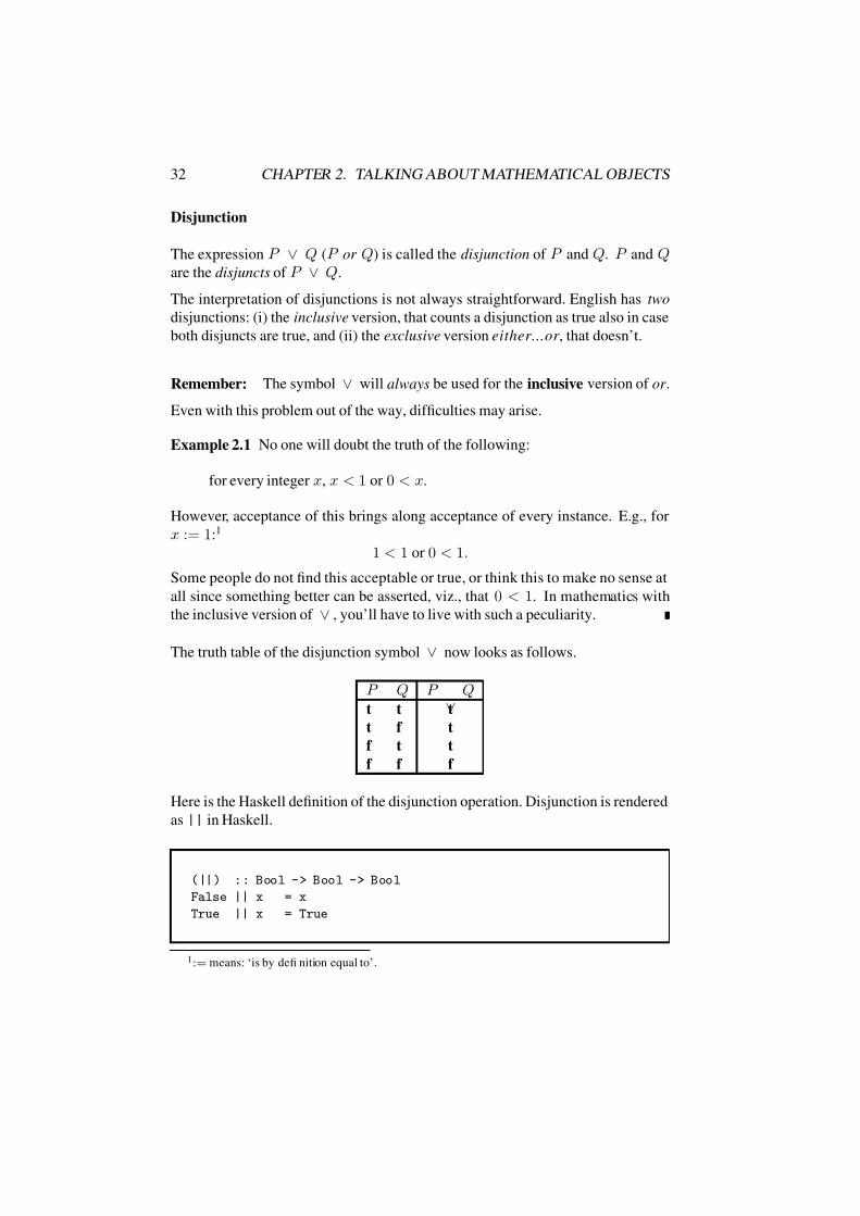
7/16/2019 The Haskell Road to Logic Maths and Programming
http://slidepdf.com/reader/full/the-haskell-road-to-logic-maths-and-programming-5634fa29ef7e9 43/448
32 CHAPTER 2. TALKING ABOUT MATHEMATICAL OBJECTS
Disjunction
The expression P ∨ Q (P or Q) is called the disjunction of P and Q. P and Qare the disjuncts of P ∨ Q.
The interpretation of disjunctions is not always straightforward. English has two
disjunctions: (i) the inclusive version, that counts a disjunction as true also in case
both disjuncts are true, and (ii) the exclusive version either...or , that doesn’t.
Remember: The symbol ∨ will always be used for the inclusive version of or .
Even with this problem out of the way, difficulties may arise.
Example 2.1 No one will doubt the truth of the following:
for every integer x, x < 1 or 0 < x.
However, acceptance of this brings along acceptance of every instance. E.g., for
x := 1:1
1 < 1 or 0 < 1.
Some people do not find this acceptable or true, or think this to make no sense at
all since something better can be asserted, viz., that 0 < 1. In mathematics with
the inclusive version of ∨ , you’ll have to live with such a peculiarity.
The truth table of the disjunction symbol ∨ now looks as follows.
P Q P ∨
Qt t t
t f t
f t t
f f f
Here is the Haskell definition of the disjunction operation. Disjunction is rendered
as || in Haskell.
(||) :: Bool -> Bool -> Bool
False || x = x
True || x = True
1:= means: ‘is by defi nition equal to’.

7/16/2019 The Haskell Road to Logic Maths and Programming
http://slidepdf.com/reader/full/the-haskell-road-to-logic-maths-and-programming-5634fa29ef7e9 44/448
2.1. LOGICAL CONNECTIVES AND THEIR MEANINGS 33
What this means is: if the first argument of a disjunction evaluates to false, then
the disjunction gets the same value as its second argument. If the first argument of a disjunction evaluates to true, then the disjunction evaluates to true.
Exercise 2.2 Make up the truth table for the exclusive version of or .
Implication
An expression of the form P ⇒ Q (if P , then Q; Q if P ) is called the implication
of P and Q. P is the antecedent of the implication and Q the consequent .
The truth table of ⇒ is perhaps the only surprising one. However, it can be moti-
vated quite simply using an example like the following. No one will disagree that
for every natural number n,
5 < n ⇒ 3 < n.
Therefore, the implication must hold in particular for n equal to 2, 4 and 6. But
then, an implication should be true if
• both antecedent and consequent are false (n = 2),
• antecedent false, consequent true (n = 4),
and
• both antecedent and consequent true (n = 6).
And of course, an implication should be false in the only remaining case that theantecedent is true and the consequent false. This accounts for the following truth
table.
P Q P ⇒ Qt t t
t f f
f t t
f f t
If we want to implement implication in Haskell, we can do so in terms of not and
||. It is convenient to introduce an infix operator ==> for this. The number 1
in the infix declaration indicates the binding power (binding power 0 is lowest,
9 is highest). A declaration of an infix operator together with an indication of its
binding power is called a fixity declaration.

7/16/2019 The Haskell Road to Logic Maths and Programming
http://slidepdf.com/reader/full/the-haskell-road-to-logic-maths-and-programming-5634fa29ef7e9 45/448
34 CHAPTER 2. TALKING ABOUT MATHEMATICAL OBJECTS
infix 1 ==>
(==>) :: Bool -> Bool -> Bool
x ==> y = (not x) || y
It is also possible to give a direct definition:
(==>) :: Bool -> Bool -> Bool
True ==> x = x
False ==> x = True
Trivially True Implications. Note that implications with antecedent false and
those with consequent true are true. For instance, because of this, the following
two sentences must be counted as true: if my name is Napoleon, then the decimal
expansion of π contains the sequence 7777777 , and: if the decimal expansion of πcontains the sequence 7777777, then strawberries are red .
Implications with one of these two properties (no matter what the values of param-
eters that may occur) are dubbed trivially true. In what follows there are quite a
number of facts that are trivial in this sense that may surprise the beginner. One is
that the empty set
∅is included in every set (cf. Theorem 4.9 p. 126).
Remark. The word trivial is often abused. Mathematicians have a habit of calling
things trivial when they are reluctant to prove them. We will try to avoid this use
of the word. The justification for calling a statement trivial resides in the psycho-
logical fact that a proof of that statement immediately comes to mind. Whether a
proof of something comes to your mind will depend on your training and experi-
ence, so what is trivial in this sense is (to some extent) a personal matter. When
we are reluctant to prove a statement, we will sometimes ask you to prove it as an
exercise.
Implication and Causality. The mathematical use of implication does not al-
ways correspond to what you are used to. In daily life you will usually require a
certain causal dependence between antecedent and consequent of an implication.
(This is the reason the previous examples look funny.) In mathematics, such a

7/16/2019 The Haskell Road to Logic Maths and Programming
http://slidepdf.com/reader/full/the-haskell-road-to-logic-maths-and-programming-5634fa29ef7e9 46/448
2.1. LOGICAL CONNECTIVES AND THEIR MEANINGS 35
causality usually will be present, but this is quite unnecessary for the interpreta-
tion of an implication: the truth table tells the complete story. (And in this sectionin particular, causality usually will be absent.) However, in a few cases, natural
language use surprisingly corresponds with truth table-meaning. E.g., I’ll be dead
if Bill will not show up must be interpreted (if uttered by someone healthy) as
strong belief that Bill will indeed turn up.2
Converse and Contraposition. The converse of an implication P ⇒ Q is Q ⇒P ; its contraposition is ¬Q ⇒ ¬P . The converse of a true implication does
not need to be true, but its contraposition is true iff the implication is. Cf. Theo-
rem 2.10, p. 45.
Necessary and Sufficient Conditions. The statement P is called a sufficient condition for Q and Q a necessary condition for P if the implication P ⇒ Qholds.
An implication P ⇒ Q can be expressed in a mathematical text in a number of
ways:
1. if P , then Q,
2. Q if P ,
3. P only if Q,
4. Q whenever P ,
5. P is sufficient for Q,6. Q is necessary for P .
Equivalence
The expression P ⇔ Q (P iff Q) is called the equivalence of P and Q. P and Qare the members of the equivalence. The truth table of the equivalence symbol is
unproblematic once you realize that an equivalence P ⇔ Q amounts to the con-
junction of two implications P ⇒ Q and Q ⇒ P taken together. (It is sometimes
convenient to write Q ⇒ P as P ⇐ Q.) The outcome is that an equivalence must
be true iff its members have the same truth value.
Table:
2‘If Bill will not show up, then I am a Dutchman’, has the same meaning, when uttered by a native
speaker of English. What it means when uttered by one of the authors of this book, we are not sure.
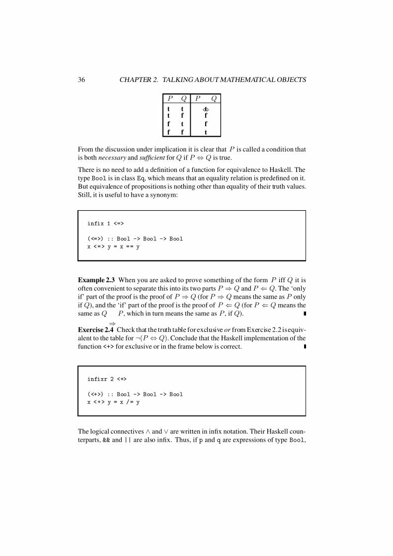
7/16/2019 The Haskell Road to Logic Maths and Programming
http://slidepdf.com/reader/full/the-haskell-road-to-logic-maths-and-programming-5634fa29ef7e9 47/448
36 CHAPTER 2. TALKING ABOUT MATHEMATICAL OBJECTS
P Q P
⇔Q
t t tt f f
f t f
f f t
From the discussion under implication it is clear that P is called a condition that
is both necessary and sufficient for Q if P ⇔ Q is true.
There is no need to add a definition of a function for equivalence to Haskell. The
type Bool is in class Eq , which means that an equality relation is predefined on it.
But equivalence of propositions is nothing other than equality of their truth values.
Still, it is useful to have a synonym:
infix 1 <=>
(<=>) :: Bool -> Bool -> Bool
x < = > y = x = = y
Example 2.3 When you are asked to prove something of the form P iff Q it is
often convenient to separate this into its two parts P ⇒ Q and P ⇐ Q. The ‘only
if’ part of the proof is the proof of P ⇒ Q (for P ⇒ Q means the same as P only
if Q), and the ‘if’ part of the proof is the proof of P ⇐ Q (for P ⇐ Q means the
same as Q
⇒P , which in turn means the same as P , if Q).
Exercise 2.4 Check that the truth table for exclusive or from Exercise 2.2 is equiv-
alent to the table for ¬(P ⇔ Q). Conclude that the Haskell implementation of the
function <+> for exclusive or in the frame below is correct.
infixr 2 <+>
(<+>) :: Bool -> Bool -> Bool
x < + > y = x / = y
The logical connectives ∧ and ∨ are written in infix notation. Their Haskell coun-
terparts, && and || are also infix. Thus, if p and q are expressions of type Bool,

7/16/2019 The Haskell Road to Logic Maths and Programming
http://slidepdf.com/reader/full/the-haskell-road-to-logic-maths-and-programming-5634fa29ef7e9 48/448
2.1. LOGICAL CONNECTIVES AND THEIR MEANINGS 37
then p & & q is a correct Haskell expression of type Bool. If one wishes to write
this in prefix notation, this is also possible, by putting parentheses around the op-erator: (&&) p q .
Although you will probably never find more than 3–5 connectives occurring in one
mathematical statement, if you insist you can use as many connectives as you like.
Of course, by means of parentheses you should indicate the way your expression
was formed.
For instance, look at the formula
¬P ∧ ((P ⇒ Q) ⇔ ¬(Q ∧ ¬P )).
Using the truth tables, you can determine its truth value if truth values for the
components P and Q have been given. For instance, if P has value t and Qhas value f , then ¬P has f , P ⇒ Q becomes f , Q ∧ ¬P : f ; ¬(Q ∧ ¬P ): t;
(P ⇒ Q) ⇔ ¬(Q ∧ ¬P ): f , and the displayed expression thus has value f . This
calculation can be given immediately under the formula, beginning with the values
given for P and Q. The final outcome is located under the conjunction symbol ∧,
which is the main connective of the expression.
¬ P ∧ ((P ⇒ Q) ⇔ ¬ (Q ∧ ¬ P ))t t f f t
f f f
f t
f
f
In compressed form, this looks as follows:
¬ P ∧ ((P ⇒ Q) ⇔ ¬ (Q ∧ ¬ P ))f t f t f f f t f f f t
Alternatively, one might use a computer to perform the calculation.

7/16/2019 The Haskell Road to Logic Maths and Programming
http://slidepdf.com/reader/full/the-haskell-road-to-logic-maths-and-programming-5634fa29ef7e9 49/448
38 CHAPTER 2. TALKING ABOUT MATHEMATICAL OBJECTS
p = Trueq = False
formula1 = (not p) && (p ==> q) <=> not (q && (not p))
After loading the file with the code of this chapter, you should be able to do:
TAMO> formula1
False
TAMO>
Note that p and q are defined as constants, with values True and False, respec-tively, so that the occurrences of p and q in the expression formula1 are evaluated
as these truth values. The rest of the evaluation is then just a matter of applying
the definitions of not, &&, <=> and ==>.
2.2 Logical Validity and Related Notions
Goal To grasp the concepts of logical validity and logical equivalence, to learn
how to use truth tables in deciding questions of validity and equivalence, and in the
handling of negations, and to learn how the truth table method for testing validity
and equivalence can be implemented.
Logical Validities. There are propositional formulas that receive the value t no
matter what the values of the occurring letters. Such formulas are called (logically)
valid .
Examples of logical validities are: P ⇒ P , P ∨ ¬P , and P ⇒ (Q ⇒ P ).
Truth Table of an Expression. If an expression contains n letters P , Q , . . ., then
there are 2n possible distributions of the truth values between these letters. The
2n-row table that contains the calculations of these values is the truth table of the
expression.
If all calculated values are equal to t, then your expression, by definition, is avalidity.

7/16/2019 The Haskell Road to Logic Maths and Programming
http://slidepdf.com/reader/full/the-haskell-road-to-logic-maths-and-programming-5634fa29ef7e9 50/448
2.2. LOGICAL VALIDITY AND RELATED NOTIONS 39
Example 2.5 (Establishing Logical Validity by Means of a Truth Table)
The following truth table shows that P ⇒ (Q ⇒ P ) is a logical validity.
P ⇒ (Q ⇒ P )t t t t t
t t f t t
f t t f f
f t f t f
To see how we can implement the validity check in Haskell, look at the imple-
mentation of the evaluation formula1 again, and add the following definition of
formula2:
formula2 p q = ((not p) && (p ==> q) <=> not (q && (not p)))
To see the difference between the two definitions, let us check their types:
TAMO> :t formula1
formula1 :: Bool
TAMO> :t formula2
formula2 :: Bool -> Bool -> Bool
TAMO>
The difference is that the first definition is a complete proposition (type Bool) in
itself, while the second still needs two arguments of type Bool before it will return
a truth value.
In the definition of formula1, the occurrences of p and q are interpreted as con-
stants, of which the values are given by previous definitions. In the definition of
formula2. the occurrences of p and q are interpreted as variables that represent
the arguments when the function gets called.
A propositional formula in which the propositionletters are interpreted as variables
can in fact be considered as a propositional function or Boolean function or truth
function. If just one variable, say p occurs in it, then it is a function of type
Bool -> Bool (takes a Boolean, returns a Boolean). If two variables occur in it,
say p and q , then it is a function of type Bool -> Bool -> Bool (takes Boolean,

7/16/2019 The Haskell Road to Logic Maths and Programming
http://slidepdf.com/reader/full/the-haskell-road-to-logic-maths-and-programming-5634fa29ef7e9 51/448
40 CHAPTER 2. TALKING ABOUT MATHEMATICAL OBJECTS
then takes another Boolean, and returns a Boolean). If three variables occur in it,
then it is of type Bool -> Bool -> Bool -> Bool, and so on.
In the validity check for a propositional formula, we treat the proposition letters
as arguments of a propositional function, and we check whether evaluation of the
function yields true for every possible combination of the arguments (that is the
essence of the truth table method for checking validity). Here is the case for propo-
sitions with one proposition letter (type Bool -> Bool).
valid1 :: (Bool -> Bool) -> Bool
valid1 bf = (bf True) && (bf False)
The validity check for Boolean functions of type Bool -> Bool is suited to test
functions of just one variable. An example is the formula P ∨ ¬P that expresses
the principle of excluded middle (or, if you prefer a Latin name, tertium non datur ,
for: there is no third possibility). Here is its implementation in Haskell:
excluded_middle :: Bool -> Bool
excluded_middle p = p || not p
To check that this is valid by the truth table method, one should consider the two
cases P := t and P := f , and ascertain that the principle yields t in both of
these cases. This is precisely what the validity check valid1 does: it yields True
precisely when applying the boolean function bf to True yields True and applying
bf to False yields True. And indeed, we get:
TAMO> valid1 excluded_middle
True
Here is the validity check for propositional functions with two proposition let-
ters, Such propositional functions have type Bool -> Bool -> Bool), and need
a truth table with four rows to check their validity, as there are four cases to check.

7/16/2019 The Haskell Road to Logic Maths and Programming
http://slidepdf.com/reader/full/the-haskell-road-to-logic-maths-and-programming-5634fa29ef7e9 52/448
2.2. LOGICAL VALIDITY AND RELATED NOTIONS 41
valid2 :: (Bool -> Bool -> Bool) -> Boolvalid2 bf = (bf True True)
&& (bf True False)
&& (bf False True)
&& (bf False False)
Again, it is easy to see that this is an implementation of the truth table method for
validity checking. Try this out on P ⇒ (Q ⇒ P ) and on (P ⇒ Q) ⇒ P , and
discover that the bracketing matters:
form1 p q = p ==> (q ==> p)
form2 p q = (p ==> q) ==> p
TAMO> valid2 form1
True
TAMO> valid2 form2
False
The propositional function formula2 that was defined above is also of the right
argument type for valid2:
TAMO> valid2 formula2
False
It should be clear how the notion of validity is to be implemented for propositional
functions with more than two propositional variables. Writing out the full tables
becomes a bit irksome, so we are fortunate that Haskell offers an alternative. We
demonstrate it in valid3 and valid4,.

7/16/2019 The Haskell Road to Logic Maths and Programming
http://slidepdf.com/reader/full/the-haskell-road-to-logic-maths-and-programming-5634fa29ef7e9 53/448
42 CHAPTER 2. TALKING ABOUT MATHEMATICAL OBJECTS
valid3 :: (Bool -> Bool -> Bool -> Bool) -> Boolvalid3 bf = and [ bf p q r | p <- [True,False],
q <- [True,False],
r <- [True,False]]
valid4 :: (Bool -> Bool -> Bool -> Bool -> Bool) -> Bool
valid4 bf = and [ bf p q r s | p <- [True,False],
q <- [True,False],
r <- [True,False],
s <- [True,False]]
The condition p <- [True,False], for “ p is an element of the list consisting of
the two truth values”, is an example of list comprehension (page 118).
The definitions make use of Haskell list notation, and of the predefined function
and for generalized conjunction. An example of a list of Booleans in Haskell is
[True,True,False]. Such a list is said to be of type [Bool]. If list is a list of
Booleans (an object of type [Bool]), then and list gives True in case all mem-
bers of list are true, False otherwise. For example, and [True,True,False]
gives False, but and [True,True,True] gives True. Further details about
working with lists can be found in Sections 4.6 and 7.5.
Leaving out Parentheses. We agree that ∧ and ∨ bind more strongly than ⇒and ⇔. Thus, for instance, P ∧ Q ⇒ R stands for (P ∧ Q) ⇒ R (and not for
P
∧(Q
⇒R)).
Operator Precedence in Haskell In Haskell, the convention is not quite the
same, for || has operator precedence 2, && has operator precedence 3, and == has
operator precedence 4, which means that == binds more strongly than &&, which
in turn binds more strongly than ||. The operators that we added, ==> and <=>,
follow the logic convention: they bind less strongly than && and ||.
Logically Equivalent. Two formulas are called (logically) equivalent if, no mat-
ter the truth values of the letters P , Q , . . . occurring in these formulas, the truth
values obtained for them are the same. This can be checked by constructing a truth
table (see Example (2.6)).
Example 2.6 (The First Law of De Morgan)
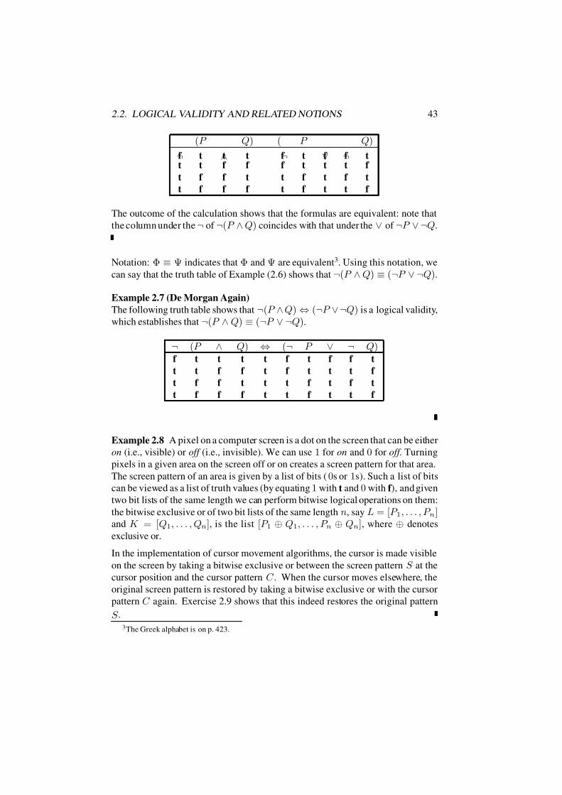
7/16/2019 The Haskell Road to Logic Maths and Programming
http://slidepdf.com/reader/full/the-haskell-road-to-logic-maths-and-programming-5634fa29ef7e9 54/448
2.2. LOGICAL VALIDITY AND RELATED NOTIONS 43
¬(P
∧Q) (
¬P
∨ ¬Q)
f t t t f t f f tt t f f f t t t f
t f f t t f t f t
t f f f t f t t f
The outcome of the calculation shows that the formulas are equivalent: note that
the column under the ¬ of ¬(P ∧ Q) coincides with that under the ∨ of ¬P ∨ ¬Q.
Notation: Φ ≡ Ψ indicates that Φ and Ψ are equivalent3. Using this notation, we
can say that the truth table of Example (2.6) shows that ¬(P ∧ Q) ≡ (¬P ∨ ¬Q).
Example 2.7 (De Morgan Again)
The following truth table shows that ¬(P ∧Q) ⇔ (¬P ∨¬Q) is a logical validity,
which establishes that ¬(P ∧ Q) ≡ (¬P ∨ ¬Q).
¬ (P ∧ Q) ⇔ (¬ P ∨ ¬ Q)f t t t t f t f f t
t t f f t f t t t f
t f f t t t f t f t
t f f f t t f t t f
Example 2.8 A pixel on a computer screen is a dot on the screen that can be either
on (i.e., visible) or off (i.e., invisible). We can use 1 for on and 0 for off . Turning
pixels in a given area on the screen off or on creates a screen pattern for that area.
The screen pattern of an area is given by a list of bits ( 0s or 1s). Such a list of bits
can be viewed as a list of truth values (by equating 1 with t and 0 with f ), and given
two bit lists of the same length we can perform bitwise logical operations on them:
the bitwise exclusive or of two bit lists of the same length n, say L = [P 1, . . . , P n]and K = [Q1, . . . , Qn], is the list [P 1 ⊕ Q1, . . . , P n ⊕ Qn], where ⊕ denotes
exclusive or.
In the implementation of cursor movement algorithms, the cursor is made visible
on the screen by taking a bitwise exclusive or between the screen pattern S at the
cursor position and the cursor pattern C . When the cursor moves elsewhere, the
original screen pattern is restored by taking a bitwise exclusive or with the cursor
pattern C again. Exercise 2.9 shows that this indeed restores the original pattern
S .3The Greek alphabet is on p. 423.

7/16/2019 The Haskell Road to Logic Maths and Programming
http://slidepdf.com/reader/full/the-haskell-road-to-logic-maths-and-programming-5634fa29ef7e9 55/448
44 CHAPTER 2. TALKING ABOUT MATHEMATICAL OBJECTS
Exercise 2.9 Let
⊕stand for exclusive or. Show, using the truth table from Exer-
cise 2.2, that (P ⊕ Q) ⊕ Q is equivalent to P .
In Haskell, logical equivalence can be tested as follows. First we give a procedure
for propositional functions with 1 parameter:
logEquiv1 :: (Bool -> Bool) -> (Bool -> Bool) -> Bool
logEquiv1 bf1 bf2 =
(bf1 True <=> bf2 True) && (bf1 False <=> bf2 False)
What this does, for formulas Φ, Ψ with a single propositional variable, is testing
the formula Φ ⇔ Ψ by the truth table method.
We can extend this to propositional functions with 2, 3 or more parameters, us-
ing generalized conjunction. Here are the implementations of logEquiv2 and
logEquiv3; it should be obvious how to extend this for truth functions with still
more arguments.
logEquiv2 :: (Bool -> Bool -> Bool) ->
(Bool -> Bool -> Bool) -> Bool
logEquiv2 bf1 bf2 =
and [(bf1 p q) <=> (bf2 p q) | p <- [True,False],
q <- [True,False]]
logEquiv3 :: (Bool -> Bool -> Bool -> Bool) ->
(Bool -> Bool -> Bool -> Bool) -> Bool
logEquiv3 bf1 bf2 =
and [(bf1 p q r) <=> (bf2 p q r) | p <- [True,False],
q <- [True,False],
r <- [True,False]]
Let us redo Exercise (2.9) by computer.
formula3 p q = p
formula4 p q = (p <+> q) <+> q

7/16/2019 The Haskell Road to Logic Maths and Programming
http://slidepdf.com/reader/full/the-haskell-road-to-logic-maths-and-programming-5634fa29ef7e9 56/448
2.2. LOGICAL VALIDITY AND RELATED NOTIONS 45
Note that the q in the definition of formula3 is needed to ensure that it is a function
with two arguments.
TAMO> logEquiv2 formula3 formula4
True
We can also test this by means of a validity check on P ⇔ ((P ⊕ Q) ⊕ Q), as
follows:
formula5 p q = p <=> ((p <+> q) <+> q)
TAMO> valid2 formula5
True
Warning. Do not confuse ≡ and ⇔. If Φ and Ψ are formulas, then Φ ≡ Ψ ex-
presses the statement that Φ and Ψ are equivalent. On the other hand, Φ ⇔ Ψ is
just another formula. The relation between the two is that the formula Φ ⇔ Ψis logically valid iff it holds that Φ ≡ Ψ. (See Exercise 2.19.) Compare the dif-
ference, in Haskell, between logEquiv2 formula3 formula4 (a true statement
about the relation between two formulas), and formula5 (just another formula).
The following theorem collects a number of useful equivalences. (Of course, P ,
Q and R can be arbitrary formulas themselves.)
Theorem 2.10 1. P 𠪪P (law of double negation),
2. P ∧ P ≡ P ; P ∨ P ≡ P (laws of idempotence),
3. (P ⇒ Q) ≡ ¬P ∨ Q;
¬(P ⇒ Q) ≡ P ∧ ¬Q ,
4. (¬P ⇒ ¬Q) ≡ (Q ⇒ P );
(P ⇒ ¬Q) ≡ (Q ⇒ ¬P );
(¬P ⇒ Q) ≡ (¬Q ⇒ P ) (laws of contraposition),
5. (P ⇔ Q) ≡ ((P ⇒ Q) ∧ (Q ⇒ P ))
≡ ((P ∧ Q) ∨ (¬P ∧ ¬Q)) ,

7/16/2019 The Haskell Road to Logic Maths and Programming
http://slidepdf.com/reader/full/the-haskell-road-to-logic-maths-and-programming-5634fa29ef7e9 57/448
46 CHAPTER 2. TALKING ABOUT MATHEMATICAL OBJECTS
6. P
∧Q
≡Q
∧P ; P
∨Q
≡Q
∨P (laws of commutativity),
7. ¬(P ∧ Q) ≡ ¬P ∨ ¬Q;
¬(P ∨ Q) ≡ ¬P ∧ ¬Q (DeMorgan laws).
8. P ∧ (Q ∧ R) ≡ (P ∧ Q) ∧ R;
P ∨ (Q ∨ R) ≡ (P ∨ Q) ∨ R (laws of associativity),
9. P ∧ (Q ∨ R) ≡ (P ∧ Q) ∨ (P ∧ R);
P ∨ (Q ∧ R) ≡ (P ∨ Q) ∧ (P ∨ R) (distribution laws),
Equivalence 8 justifies leaving out parentheses in conjunctions and disjunctions of
three or more conjuncts resp., disjuncts. Non-trivial equivalences that often are
used in practice are 2, 3 and 9. Note how you can use these to re-write negations:
a negation of an implication can be rewritten as a conjunction, a negation of a
conjunction (disjunction) is a disjunction (conjunction).
Exercise 2.11 The First Law of De Morgan was proved in Example 2.6. This
method was implemented above. Use the method by hand to prove the other parts
of Theorem 2.10.
We will now demonstrate how one can use the implementation of the logical equiv-
alence tests as a check for Theorem 2.10. Here is a question for you to ponder:
does checking the formulas by means of the implemented functions for logical
equivalence count as a proof of the principles involved? Whatever the answer to
this one may be, Figure 2.1 defines the tests for the statements made in Theorem
2.10, by means of lambda abstraction The expression \ p -> not (not p) isthe Haskell way of referring to the lambda term λp.¬¬ p, the term that denotes the
operation of performing a double negation. See Section 2.4.
If you run these tests, you get result True for all of them. E.g.:
TAMO> test5a
True
The next theorem lists some useful principles for reasoning with (the proposition
that is always true; the Haskell counterpart is True) and ⊥ (the proposition that is
always false; the Haskell counterpart of this is False).
Theorem 2.12 1. ¬ ≡ ⊥; ¬ ⊥ ≡ ,
2. P ⇒ ⊥ ≡ ¬P ,

7/16/2019 The Haskell Road to Logic Maths and Programming
http://slidepdf.com/reader/full/the-haskell-road-to-logic-maths-and-programming-5634fa29ef7e9 58/448
2.2. LOGICAL VALIDITY AND RELATED NOTIONS 47
test1 = logEquiv1 id (\ p -> not (not p))
test2a = logEquiv1 id (\ p -> p && p)
test2b = logEquiv1 id (\ p -> p || p)
test3a = logEquiv2 (\ p q -> p ==> q) (\ p q -> not p || q)
test3b = logEquiv2 (\ p q -> not (p ==> q)) (\ p q -> p && not q)
test4a = logEquiv2 (\ p q -> not p ==> not q) (\ p q -> q ==> p)
test4b = logEquiv2 (\ p q -> p ==> not q) (\ p q -> q ==> not p)test4c = logEquiv2 (\ p q -> not p ==> q) (\ p q -> not q ==> p)
test5a = logEquiv2 (\ p q -> p <=> q)
(\ p q -> (p ==> q) && (q ==> p))
test5b = logEquiv2 (\ p q -> p <=> q)
(\ p q -> (p && q) || (not p && not q))
test6a = logEquiv2 (\ p q -> p && q) (\ p q -> q && p)
test6b = logEquiv2 (\ p q -> p || q) (\ p q -> q || p)
test7a = logEquiv2 (\ p q -> not (p && q))
(\ p q -> not p || not q)
test7b = logEquiv2 (\ p q -> not (p || q))
(\ p q -> not p && not q)
test8a = logEquiv3 (\ p q r -> p && (q && r))
(\ p q r -> (p && q) && r)
test8b = logEquiv3 (\ p q r -> p || (q || r))(\ p q r -> (p || q) || r)
test9a = logEquiv3 (\ p q r -> p && (q || r))
(\ p q r -> (p && q) || (p && r))
test9b = logEquiv3 (\ p q r -> p || (q && r))
(\ p q r -> (p || q) && (p || r))
Figure 2.1: Defining the Tests for Theorem 2.10.

7/16/2019 The Haskell Road to Logic Maths and Programming
http://slidepdf.com/reader/full/the-haskell-road-to-logic-maths-and-programming-5634fa29ef7e9 59/448
48 CHAPTER 2. TALKING ABOUT MATHEMATICAL OBJECTS
3. P
∨ ≡ ; P
∧ ⊥ ≡ ⊥(dominance laws),
4. P ∨ ⊥ ≡ P ; P ∧ ≡ P (identity laws),
5. P ∨ ¬P ≡ (law of excluded middle),
6. P ∧ ¬P ≡ ⊥ (contradiction).
Exercise 2.13 Implement checks for the principles from Theorem 2.12.
Without proof, we state the following Substitution Principle: If Φ and Ψ are
equivalent, and Φ and Ψ are the results of substituting Ξ for every occurrence of
P in Φ and in Ψ, respectively, then Φ and Ψ are equivalent. Example 2.14 makes
clear what this means.
Example 2.14 From ¬(P ⇒ Q) ≡ P ∧ ¬Q plus the substitution principle it
follows that
¬(¬P ⇒ Q) ≡ ¬P ∧ ¬Q
(by substituting ¬P for P ), but also that
¬(a = 2b − 1 ⇒ a is prime) ≡ a = 2b − 1 ∧ a is not prime
(by substituting a = 2b − 1 for P and a is prime for Q).
Exercise 2.15 A propositional contradiction is a formula that yields false for every
combination of truth values for its proposition letters. Write Haskell definitions of
contradiction tests for propositional functions with one, two and three variables.
Exercise 2.16 Produce useful denials for every sentence of Exercise 2.31. (A de-
nial of Φ is an equivalent of ¬Φ.)
Exercise 2.17 Produce a denial for the statement that x < y < z (where x,y,z ∈R).
Exercise 2.18 Show:
1. (Φ ⇔ Ψ) ≡ (¬Φ ⇔ ¬Ψ),
2. (¬Φ ⇔ Ψ) ≡ (Φ ⇔ ¬Ψ).
Exercise 2.19 Show that Φ ≡ Ψ is true iff Φ ⇔ Ψ is logically valid.

7/16/2019 The Haskell Road to Logic Maths and Programming
http://slidepdf.com/reader/full/the-haskell-road-to-logic-maths-and-programming-5634fa29ef7e9 60/448
2.2. LOGICAL VALIDITY AND RELATED NOTIONS 49
Exercise 2.20 Determine (either using truth tables or Theorem 2.10) which of the
following are equivalent, next check your answer by computer:
1. ¬P ⇒ Q and P ⇒ ¬Q,
2. ¬P ⇒ Q and Q ⇒ ¬P ,
3. ¬P ⇒ Q and ¬Q ⇒ P ,
4. P ⇒ (Q ⇒ R) and Q ⇒ (P ⇒ R),
5. P ⇒ (Q ⇒ R) and (P ⇒ Q) ⇒ R,
6. (P ⇒ Q) ⇒ P and P ,
7. P ∨ Q ⇒ R and (P ⇒ R) ∧ (Q ⇒ R).
Exercise 2.21 Answer as many of the following questions as you can:
1. Construct a formula Φ involving the letters P and Q that has the following
truth table.
P Q Φt t t
t f t
f t f
f f t
2. How many truth tables are there for 2-letter formulas altogether?
3. Can you find formulas for all of them?
4. Is there a general method for finding these formulas?
5. And what about 3-letter formulas and more?
7/16/2019 The Haskell Road to Logic Maths and Programming
http://slidepdf.com/reader/full/the-haskell-road-to-logic-maths-and-programming-5634fa29ef7e9 61/448
50 CHAPTER 2. TALKING ABOUT MATHEMATICAL OBJECTS
2.3 Making Symbolic Form Explicit
In a sense, propositional reasoning is not immediately relevant for mathematics.
Few mathematicians will ever feel the urge to write down a disjunction of two
statements like 3 < 1 ∨ 1 < 3. In cases like this it is clearly “better” to only write
down the right-most disjunct.
Fortunately, once variables enter the scene, propositional reasoning suddenly be-
comes a very useful tool: the connectives turn out to be quite useful for combining
open formulas. An open formula is a formula with one or more unbound variables
in it. Variable binding will be explained below, but here is a first example of a
formula with an unbound variable x. A disjunction like 3 < x ∨ x < 3 is (in some
cases) a useful way of expressing that x = 3.
Example. Consider the following (true) sentence:
Between every two rational numbers there is a third one. (2.1)
The property expressed in (2.1) is usually referred to as density of the rationals.
We will take a systematic look at proving such statements in Chapter 3.
Exercise 2.22 Can you think of an argument showing that statement (2.1) is true?
A Pattern. There is a logical pattern underlying sentence (2.1). To make it visi-
ble, look at the following, more explicit, formulation. It uses variables x, y and z
for arbitrary rationals, and refers to the ordering < ofthe setQ of rational numbers.
For all rational numbers x and z, if x < z, then some (2.2)
rational number y exists such that x < y and y < z.
You will often find ‘x < y and y < z ’ shortened to: x < y < z.
Quantifiers Note the words all (or: for all), some (or: for some, some. . . exists,
there exists. . . such that , etc.). They are called quantifiers, and we use the symbols
∀ and ∃ as shorthands for them.
With these shorthands, plus the shorthands for the connectives that we saw above,
and the shorthand . . . ∈ Q for the property of being a rational, we arrive at the
following compact symbolic formulation:
∀x∈Q ∀z ∈Q ( x < z ⇒ ∃y ∈Q ( x < y ∧ y < z ) ). (2.3)

7/16/2019 The Haskell Road to Logic Maths and Programming
http://slidepdf.com/reader/full/the-haskell-road-to-logic-maths-and-programming-5634fa29ef7e9 62/448
2.3. MAKING SYMBOLIC FORM EXPLICIT 51
We will use example (2.3) to make a few points about the proper use of the vocab-
ulary of logical symbols. An expression like (2.3) is called a sentence or a formula.Note that the example formula (2.3) is composite: we can think of it as constructed
out of simpler parts. We can picture its structure as in Figure (2.2).
∀x ∈ Q∀z ∈ Q(x < z ⇒ ∃y ∈ Q(x < y ∧ y < z ))
∀z ∈ Q(x < z ⇒ ∃y ∈ Q(x < y ∧ y < z ))
(x < z ⇒ ∃y ∈ Q(x < y ∧ y < z ))
x < z
∃y
∈Q(x < y
∧y < z)
(x < y ∧ y < z)
x < y y < z
Figure 2.2: Composition of Example Formula from its Sub-formulas.
As the figure shows, the example formula is formed by putting the quantifier prefix
∀x ∈ Q in front of the result of putting quantifier prefix ∀z ∈ Q in front of a
simpler formula, and so on.
The two consecutive universalquantifier prefixes can also be combined into ∀x, z ∈Q. This gives the phrasing
∀x, z ∈ Q( x < z ⇒ ∃y ∈Q ( x < y ∧ y < z ) ).
Putting an ∧ between the two quantifiers is incorrect, however. In other words, the
expression ∀x ∈Q ∧ ∀z ∈Q(x < z ⇒ ∃y ∈Q(x < y ∧ y < z)) is considered
ungrammatical. The reason is that the formula part ∀x ∈ Q is itself not a formula,
but a prefix that turns a formula into a more complex formula. The connective ∧can only be used to construct a new formula out of two simpler formulas, so ∧cannot serve to construct a formula from ∀x ∈ Q and another formula.
The symbolic version of the density statement uses parentheses. Their function is
to indicate the way the expression has been formed and thereby to show the scope
of operators. The scope of a quantifier-expression is the formula that it combines
with to form a more complex formula. The scopes of quantifier-expressions and
connectives in a formula are illustrated in the structure tree of that formula. Figure

7/16/2019 The Haskell Road to Logic Maths and Programming
http://slidepdf.com/reader/full/the-haskell-road-to-logic-maths-and-programming-5634fa29ef7e9 63/448
52 CHAPTER 2. TALKING ABOUT MATHEMATICAL OBJECTS
2.2 shows that the scope of the quantifier-expression
∀x
∈Q is the formula
∀z ∈ Q(x < z ⇒ ∃y ∈ Q (x < y ∧ y < z )),
the scope of ∀z ∈ Q is the formula
(x < z ⇒ ∃y ∈ Q(x < y ∧ y < z)),
and the scope of ∃y ∈ Q is the formula (x < y ∧ y < z).
Exercise 2.23 Give structure trees of the following formulas (we use shorthand
notation, and write A(x) as Ax for readability).
1. ∀x(Ax ⇒ (Bx ⇒ Cx)).
2. ∃x(Ax ∧ Bx).
3. ∃xAx ∧ ∃xBx.
The expression for all (and similar ones) and its shorthand, the symbol ∀, is called
the universal quantifier ; the expression there exists (and similar ones) and its short-
hand, the symbol ∃, is called the existential quantifier . The letters x, y and z that
have been used in combination with them are variables. Note that ‘for some’ is
equivalent to ‘for at least one’.
Unrestricted and Restricted Quantifiers, Domain of Quantification Quanti-fiers can occur unrestricted : ∀x(x 0), ∃y∀x(y > x), and restricted : ∀x ∈A(x 0), ∃y ∈ B(y < a) (where A and B are sets).
In the unrestricted case, there should be some domain of quantification that often
is implicit in the context. E.g., if the context is real analysis, ∀x may mean for all
reals x. . . , and ∀f may mean for all real-valued functions f . . . .
Example 2.24 R is the set of real numbers. The fact that the R has no greatest
element can be expressed with restricted quantifiers as:
∀x ∈ R∃y ∈ R(x < y).
If we specify that all quantifiers range over the reals (i.e., if we say that R is the
domain of quantification) then we can drop the explicit restrictions, and we get by
with ∀x∃y(x < y ).

7/16/2019 The Haskell Road to Logic Maths and Programming
http://slidepdf.com/reader/full/the-haskell-road-to-logic-maths-and-programming-5634fa29ef7e9 64/448
2.3. MAKING SYMBOLIC FORM EXPLICIT 53
The use of restricted quantifiers allows for greater flexibility, for it permits one to
indicate different domains for different quantifiers.
Example 2.25
∀x ∈ R∀y ∈ R(x < y ⇒ ∃z ∈ Q (x < z < y)).
Instead of ∃x(Ax ∧ . . .) one can write ∃x ∈ A(. . .). The advantage when all
quantifiers are thus restricted is that it becomes immediately clear that the domain
is subdivided into different sub domains or types. This can make the logical
translation much easier to comprehend.
Remark. We will use standard names for the following domains: N for the natural
numbers,Z for the integer numbers,Q for the rational numbers, and R for the real
numbers. More information about these domains can be found in Chapter 8.
Exercise 2.26 Write as formulas with restricted quantifiers:
1. ∃x∃y(x ∈ Q ∧ y ∈ Q ∧ x < y).
2. ∀x(x ∈ R ⇒ ∃y(y ∈ R ∧ x < y)).
3. ∀x(x ∈ Z ⇒ ∃m, n(m ∈ N ∧ n ∈ N ∧ x = m − n)).
Exercise 2.27 Write as formulas without restricted quantifiers:
1. ∀x ∈ Q∃m, n ∈ Z(n = 0 ∧ x = m/n).
2. ∀x ∈ F ∀y ∈ D(Oxy ⇒ Bxy).
Bound Variables. Quantifier expressions ∀x, ∃y,. . . (and their restricted com-
panions) are said to bind every occurrence of x, y,. . . in their scope. If a variable
occurs bound in a certain expression then the meaning of that expression does not
change when all bound occurrences of that variable are replaced by another one.

7/16/2019 The Haskell Road to Logic Maths and Programming
http://slidepdf.com/reader/full/the-haskell-road-to-logic-maths-and-programming-5634fa29ef7e9 65/448
54 CHAPTER 2. TALKING ABOUT MATHEMATICAL OBJECTS
Example 2.28
∃y
∈Q(x < y) has the same meaning as
∃z
∈Q(x < z).
This indicates that y is bound in ∃y ∈ Q(x < y). But ∃y ∈ Q(x < y) and∃y ∈ Q(z < y) have different meanings, for the first asserts that there exists a ra-
tional number greater than some given number x, and the second that there exists
a rational number greater than some given z.
Universal and existential quantifiers are not the only variable binding operators
used by mathematicians. There are several other constructs that you are probably
familiar with which can bind variables.
Example 2.29 (Summation, Integration.) The expression5
i=1 i is nothing but
a way to describe the number 15 (15 = 1 + 2 + 3 + 4 + 5), and clearly, 15 does
in no way depend on i. Use of a different variable does not change the meaning:
5
k=1
k = 15. Here are the Haskell versions:
Prelude> sum [ i | i <- [1..5] ]
15
Prelude> sum [ k | k <- [1..5] ]
15
Similarly, the expression 1
0xdx denotes the number 1
2 and does not depend on x.
Example 2.30 (Abstraction.) Another way to bind a variable occurs in the ab-
straction notation x ∈ A | P , cf. (4.1), p. 118. The Haskell counterpart to this
is list comprehension:
[ x | x <- list, property x ]
The choice of variable does not matter. The same list is specified by:
[ y | y <- list, property y ]
The way set comprehension is used to define sets is similar to the way list compre-
hension is used to define lists, and this is similar again to the way lambda abstrac-
tion is used to define functions. See 2.4.

7/16/2019 The Haskell Road to Logic Maths and Programming
http://slidepdf.com/reader/full/the-haskell-road-to-logic-maths-and-programming-5634fa29ef7e9 66/448
2.3. MAKING SYMBOLIC FORM EXPLICIT 55
Bad Habits. It is not unusualto encounterour example-statement (2.1) displayed
as follows.
For all rationals x and y , if x < y , then both x < z and z < y hold
for some rational z.
Note that the meaning of this is not completely clear. With this expression the true
statement that ∀x, y∈Q∃z ∈Q (x < y ⇒ (x < z ∧ z < y )) could be meant, but
what also could be meant is the false statement that ∃z ∈Q ∀x, y ∈Q (x < y ⇒(x < z ∧ z < y)).
Putting quantifiers both at the front and at the back of a formula results in ambigu-
ity, for it becomes difficult to determine their scopes. In the worst case the result
is an ambiguity between statements that mean entirely different things.
It does not look too well to let a quantifier bind an expression that is not a variable,
such as in:
for all numbers n2 + 1 , . . .
Although this habit does not always lead to unclarity, it is better to avoid it, as
the result is often rather hard to comprehend. If you insist on quantifying over
complex terms, then the following phrasing is suggested: for all numbers of the
form n2 + 1, . . .
Of course, in the implementation language, terms like n + 1 are important for
pattern matching.
Translation Problems. It is easy to find examples of English sentences that are
hard to translate into the logical vernacular. E.g., in between two rationals is a
third one it is difficult to discover a universal quantifier and an implication.
Also, sometimes the English has an indefinite article where the meaning is clearly
universal. Consider the sentence a well-behaved child is a quiet child . The indef-
inite articles here may suggest existential quantifiers; however, the reading that is
clearly meant has the form
∀x ∈ C (Well-behaved(x) ⇒ Quiet(x)).
A famous example from philosophy of language is: if a farmer owns a donkey, he
beats it . Again, in spite of the indefinite articles, the meaning is universal:
∀x∀y((Farmer(x) ∧ Donkey(y) ∧ Own(x, y)) ⇒ Beat(x, y)).
7/16/2019 The Haskell Road to Logic Maths and Programming
http://slidepdf.com/reader/full/the-haskell-road-to-logic-maths-and-programming-5634fa29ef7e9 67/448
56 CHAPTER 2. TALKING ABOUT MATHEMATICAL OBJECTS
In cases like this, translation into a formula reveals the logical meaning that re-
mained hidden in the original phrasing.
In mathematical texts it also occurs quite often that the indefinite article a is used to
make universal statements. Compare Example (2.43) below, where the following
universal statement is made: A real function is continuous if it satisfies the ε-δ -definition.
Exercise 2.31 Translate into formulas, taking care to express the intended mean-
ing:
1. The equation x2 + 1 = 0 has a solution.
2. A largest natural number does not exist.
3. The number 13 is prime (use d|n for ‘d divides n’).4. The number n is prime.
5. There are infinitely many primes.
Exercise 2.32 Translate into formulas:
1. Everyone loved Diana. (Use the expression L(x, y) for: x loved y, and the
name d for Diana.)
2. Diana loved everyone.
3. Man is mortal. (Use M (x) for ‘x is a man’, and M’(x) for ‘x is mortal’.)4. Some birds do not fly. (Use B(x) for ‘x is a bird’ and F (x) for ‘x can fly’.)
Exercise 2.33 Translate into formulas, using appropriate expressions for the pred-
icates:
1. Dogs that bark do not bite.
2. All that glitters is not gold.
3. Friends of Diana’s friends are her friends.
4.*The limit of
1
n as n approaches infinity is zero.

7/16/2019 The Haskell Road to Logic Maths and Programming
http://slidepdf.com/reader/full/the-haskell-road-to-logic-maths-and-programming-5634fa29ef7e9 68/448
2.3. MAKING SYMBOLIC FORM EXPLICIT 57
Expressing Uniqueness. If we combine quantifiers with the relation = of iden-
tity, we can make definite statements like ‘there is precisely one real number xwith the property that for any real number y, xy = y’. The logical rendering is
(assuming that the domain of discussion is R):
∃x(∀y(x · y = y) ∧ ∀z(∀y(z · y = y) ⇒ z = x)).
The first part of this formula expresses that at least one x satisfies the property
∀y(x · y = y), and the second part states that any z satisfying the same property is
identical to that x.
The logical structure becomes more transparent if we write P for the property.
This gives the following translation for ‘precisely one object has property P ’:
∃x(P x
∧ ∀z(P z
⇒z = x)).
Exercise 2.34 Use the identity symbol = to translate the following sentences:
1. Everyone loved Diana except Charles.
2. Every man adores at least two women.
3. No man is married to more than one woman.
Long ago the philosopher Bertrand Russell has proposed this logical format for the
translation of the English definite article. According to his theory of description,
the translation of The King is raging becomes:
∃x(King(x) ∧ ∀y(King(y) ⇒ y = x) ∧ Raging(x)).
Exercise 2.35 Use Russell’s recipe to translate the following sentences:
1. The King is not raging.
2. The King is loved by all his subjects. (use K (x) for ‘x is a King’, and
S (x, y) for ‘x is a subject of y’).
Exercise 2.36 Translate the following logical statements back into English.
1. ∃x ∈ R(x2 = 5).

7/16/2019 The Haskell Road to Logic Maths and Programming
http://slidepdf.com/reader/full/the-haskell-road-to-logic-maths-and-programming-5634fa29ef7e9 69/448
58 CHAPTER 2. TALKING ABOUT MATHEMATICAL OBJECTS
2.
∀n
∈N
∃m
∈N(n < m).
3. ∀n ∈ N¬∃d ∈ N(1 < d < (2n + 1) ∧ d|(2n + 1)).
4. ∀n ∈ N∃m ∈ N(n < m ∧ ∀ p ∈ N( p n ∨ m p)).
5. ∀ε ∈ R+∃n ∈ N∀m ∈ N(m n ⇒ (|a − am| ε)). (R+ is the set of
positive reals; a, a0, a1, . . . refer to real numbers .)
Remark. Note that translating back and forth between formulas and plain English
involves making decisions about a domain of quantification and about the predi-
cates to use. This is often a matter of taste. For instance, how does one choose
between P (n) for ‘n is prime’ and the spelled out
n > 1 ∧ ¬∃d ∈ N(1 < d < n ∧ d|n),
which expands the definition of being prime? Expanding the definitions of mathe-
matical concepts is not always a good idea. The purpose of introducing the word
prime was precisely to hide the details of the definition, so that they do not bur-
den the mind. The art of finding the right mathematical phrasing is to introduce
precisely the amount and the kind of complexity that are needed to handle a given
problem.
Before we will start looking at the language of mathematics and its conventions in
a more systematic way, we will make the link between mathematical definitions
and implementations of those definitions.
2.4 Lambda Abstraction
The following description defines a specific function that does not depend at all on
x:
The function that sends x to x2.
Often used notations are x → x2 and λx.x2. The expression λx.x2 is called a
lambda term.
If t is an expression of type b and x is a variable of type a then λx.t is an expression
of type a → b, i.e., λx.t denotes a function. This way of defining functions is
called lambda abstraction.

7/16/2019 The Haskell Road to Logic Maths and Programming
http://slidepdf.com/reader/full/the-haskell-road-to-logic-maths-and-programming-5634fa29ef7e9 70/448
2.4. LAMBDA ABSTRACTION 59
Note that the function that sends y to y2 (notation y
→y2, or λy.y2) describes the
same function as λx.x2.
In Haskell, function definition by lambda abstraction is available. Compare the
following two definitions:
square1 :: Integer -> Integer
square1 x = x^2
square2 :: Integer -> Integer
square2 = \ x -> x^2
In the first of these, the parameter x is given as an argument. In the second, the
function is defined as a lambda abstract. The Haskell way of lambda abstraction
goes like this. The syntax is: \ v -> body, where v is a variable of the argu-
ment type and body an expression of the result type. It is allowed to abbreviate
\ v -> \ w -> body to \ v w -> body. And so on, for more than two vari-
ables. E.g., both of the following are correct:
m1 :: Integer -> Integer -> Integer
m1 = \ x -> \ y -> x*y
m2 :: Integer -> Integer -> Integer
m2 = \ x y -> x*y
And again, the choice of variables does not matter.
Also, it is possible to abstract over tuples. Compare the following definition of a
function that solves quadraticequations by means of the well-known ‘abc’-formula
x =−b ± √
b2 − 4ac
2a
.

7/16/2019 The Haskell Road to Logic Maths and Programming
http://slidepdf.com/reader/full/the-haskell-road-to-logic-maths-and-programming-5634fa29ef7e9 71/448
60 CHAPTER 2. TALKING ABOUT MATHEMATICAL OBJECTS
solveQdr :: (Float,Float,Float) -> (Float,Float)solveQdr = \ (a,b,c) -> if a == 0 then error "not quadratic"
else let d = b^2 - 4*a*c in
if d < 0 then error "no real solutions"
else
((- b + sqrt d) / 2*a,
(- b - sqrt d) / 2*a)
To solve the equation x2 − x − 1 = 0, use solveQdr (1,-1,-1), and you will
get the (approximately correct) answer (1.61803,-0.618034). Approximately
correct, for 1.61803 is an approximation of the golden ratio, 1+√
52 , and −0.618034
is an approximation of 1−√ 52 .
One way to think about quantified expressions like ∀xP x and ∃yP y is as com-
binations of a quantifier expression ∀ or ∃ and a lambda term λx.Px or λy.Py.
The lambda abstract λx.Px denotes the property of being a P . The quantifier ∀is a function that maps properties to truth values according to the recipe: if the
property holds of the whole domain then t, else f . The quantifier ∃ is a function
that maps properties to truth values according to the recipe: if the property holds
of anything at all then t, else f . This perspective on quantification is the basis of
the Haskell implementation of quantifiers in Section 2.8.
2.5 Definitions and Implementations
Here is an example of a definition in mathematics. A natural number n is prime if
n > 1 and no number m with 1 < m < n divides n.
We can capture this definition of being prime in a formula, using m|n for ‘mdivides n’, as follows (we assume the natural numbers as our domain of discourse):
n > 1 ∧ ¬∃m(1 < m < n ∧ m|n). (2.4)
Another way of expressing this is the following:
n > 1 ∧ ∀m((1 < m < n) ⇒ ¬m|n). (2.5)
If you have trouble seeing that formulas (2.4) and (2.5) mean the same, don’t
worry. We will study such equivalences between formulas in the course of this
chapter.

7/16/2019 The Haskell Road to Logic Maths and Programming
http://slidepdf.com/reader/full/the-haskell-road-to-logic-maths-and-programming-5634fa29ef7e9 72/448
2.6. ABSTRACT FORMULAS AND CONCRETE STRUCTURES 61
If we take the domain of discourse to be the domain of the natural numbers N =
0, 1, 2, . . ., then formula (2.5) expresses that n is a prime number.
We can make the fact that the formula is meant as a definition explicit by introduc-
ing a predicate name P and linking that to the formula:4
P (n) :≡ n > 1 ∧ ∀m((1 < m < n) ⇒ ¬m|n). (2.6)
One way to think about this definition is as a procedure for testing whether a
natural number is prime. Is 83 a prime? Yes, because none of 2, 3, 4, . . . , 9 divides
83. Note that there is no reason to check 10, . . ., for since 10 × 10 > 83 any factor
m of 83 with m 10 will not be the smallest factor of 83, and a smaller factor
should have turned up before.
The example shows that we can make the prime procedure more efficient. We only
have to try and find the smallest factor of n, and any b with b2 > n cannot be the
smallest factor. For suppose that a number b with b2 n divides n. Then there is
a number a with a × b = n, and therefore a2 n, and a divides n. Our definition
can therefore run:
P (n) :≡ n > 1 ∧ ∀m((1 < m ∧ m2 n) ⇒ ¬m|n). (2.7)
In Chapter 1 we have seen that this definition is equivalent to the following:
P (n) :≡ n > 1 ∧ LD(n) = n. (2.8)
The Haskell implementation of the primality test was given in Chapter 1.
2.6 Abstract Formulas and Concrete Structures
The formulas of Section 2.1 are “handled” using truth values and tables. Quan-
tificational formulas need a structure to become meaningful. Logical sentences
involving variables can be interpreted in quite different structures. A structure
is a domain of quantification, together with a meaning for the abstract symbols
that occur. A meaningful statement is the result of interpreting a logical formula
in a certain structure. It may well occur that interpreting a given formula in one
structure yields a true statement, while interpreting the same formula in a differ-
ent structure yields a false statement. This illustrates the fact that we can use one
logical formula for many different purposes.
Look again at the example-formula (2.3), now displayed without reference to Q
and using a neutral symbolR. This gives:
∀x ∀y ( xRy =⇒ ∃z ( xRz ∧ zRy ) ). (2.9)
4:≡means: ‘is by defi nition equivalent to’.

7/16/2019 The Haskell Road to Logic Maths and Programming
http://slidepdf.com/reader/full/the-haskell-road-to-logic-maths-and-programming-5634fa29ef7e9 73/448
62 CHAPTER 2. TALKING ABOUT MATHEMATICAL OBJECTS
It is only possible to read this as a meaningful statement if
1. it is understood which is the underlying domain of quantification,
and
2. what the symbolR stands for.
Earlier, the set of rationals Q was used as the domain, and the ordering < was
employed instead of the —in itself meaningless— symbol R. In the context of Q
and <, the quantifiers ∀x and ∃z in (2.9) should be read as: for all rationals x . . . ,
resp., for some rational z . . . , whereasR should be viewed as standing for <. In
that particular case, the formula expresses the true statement that, between every
two rationals, there is a third one.
However, one can also choose the set N = 0, 1, 2, . . . of natural numbers as
domain and the corresponding ordering < as the meaning of R. In that case,
the formula expresses the false statement that between every two natural numbers
there is a third one.
A specification of (i) a domain of quantification, to make an unrestricted use of the
quantifiers meaningful, and (ii) a meaning for the unspecified symbols that may
occur (here: R), will be called a context or a structure for a given formula.
As you have seen here: given such a context, the formula can be “read” as a
meaningful assertion about this context that can be either true or false.
Open Formulas, Free Variables, and Satisfaction. If one deletes the first quan-
tifier expression ∀x from the example formula (2.9), then the following remains:
∀y ( xRy =⇒ ∃z ( xRz ∧ zRy ) ). (2.10)
Although this expression does have the form of a statement, it in fact is not such a
thing. Reason: statements are either true or false; and, even if a quantifier domain
and a meaning forR were specified, what results cannot be said to be true or false,
as long as we do not know what it is that the variable x (which no longer is bound
by the quantifier ∀x) stands for.
However, the expression can be turned into a statement again by replacing the
variable x by (the name of) some object in the domain, or —what amounts to the
same— by agreeing that x denotes this object.
For instance, if the domain consists of the set N ∪ q ∈ Q | 0 < q < 1 of natural
numbers together with all rationals between 0 and 1, and the meaning of R is the

7/16/2019 The Haskell Road to Logic Maths and Programming
http://slidepdf.com/reader/full/the-haskell-road-to-logic-maths-and-programming-5634fa29ef7e9 74/448
2.6. ABSTRACT FORMULAS AND CONCRETE STRUCTURES 63
usual ordering relation < for these objects, then the expression turns into a truth
upon replacing x by 0.5 or by assigning x this value. We say that 0.5 satisfies theformula in the given domain.
However, (2.10) turns into a falsity when we assign 2 to x; in other words, 2 does
not satisfy the formula.
Of course, one can delete a next quantifier as well, obtaining:
xRy =⇒ ∃z ( xRz ∧ zRy ).
Now, both x and y have become free, and, next to a context, values have to be
assigned to both these variables in order to determine a truth value.
An occurrence of a variable in an expression that is not (any more) in the scope of a
quantifier is said to be free in that expression. Formulas that contain free variables
are called open.
An open formula can be turned into a statement in two ways: (i) adding quantifiers
that bind the free variables; (ii) replacing the free variables by (names of) objects
in the domain (or stipulating that they have such objects as values).
Exercise 2.37 Consider the following formulas.
1. ∀x∀y(xRy),
2. ∀x∃y(xRy).
3. ∃x∀y(xRy).
4. ∃x∀y(x = y ∨ xRy).
5. ∀x∃y(xRy ∧ ¬∃z(xRz ∧ zRy)).
Are these formulas true or false in the following contexts?:
a. Domain: N = 0, 1, 2, . . .; meaning of R: <,
b. Domain: N; meaning of R: >,
c. Domain: Q (the set of rationals); meaning of R: <,
d. Domain: R (the set of reals); meaning of xRy: y2 = x,
e. Domain: set of all human beings; meaning of R: father-of,
f. Domain: set of all human beings; meaning of xRy: x loves y.

7/16/2019 The Haskell Road to Logic Maths and Programming
http://slidepdf.com/reader/full/the-haskell-road-to-logic-maths-and-programming-5634fa29ef7e9 75/448
64 CHAPTER 2. TALKING ABOUT MATHEMATICAL OBJECTS
Exercise 2.38 In Exercise 2.37, delete the first quantifier on x in formulas 1–5.
Determine for which values of x the resulting open formulas are satisfied in each
of the structures a–f.
2.7 Logical Handling of the Quantifiers
Goal To learn how to recognize simple logical equivalents involving quantifiers,
and how to manipulate negations in quantified contexts.
Validities and Equivalents. Compare the corresponding definitionsin Section 2.2.
1. A logical formula is called (logically) valid if it turns out to be true in every
structure.
2. Formulas are (logically) equivalent if they obtain the same truth value in
every structure (i.e., if there is no structure in which one of them is true and
the other one is false).
Notation: Φ ≡ Ψ expresses that the quantificational formulas Φ and Ψ are
equivalent.
Exercise 2.39 (The propositional version of this is in Exercise 2.19 p. 48.) Argue
that Φ and Ψ are equivalent iff Φ ⇔ Ψ is valid.
Because of the reference to every possible structure (of which there are infinitely
many), these are quite complicated definitions, and it is nowhere suggested that
you will be expected to decide on validity or equivalence in every case that you
may encounter. In fact, in 1936 it was provedrigorously, by Alonzo Church (1903–
1995) and Alan Turing (1912–1954) that no one can! This illustrates that the
complexity of quantifiers exceeds that of the logic of connectives, where truth
tables allow you to decide on such things in a mechanical way, as is witnessed
by the Haskell functions that implement the equivalence checks for propositional
logic.
Nevertheless: the next theorem already shows that it is sometimes very well possi-
ble to recognize whether formulas are valid or equivalent — if only these formulas
are sufficiently simple.
Only a few useful equivalents are listed next. Here, Ψ(x), Φ(x, y) and the like
denote logical formulas that may contain variables x (or x, y) free.

7/16/2019 The Haskell Road to Logic Maths and Programming
http://slidepdf.com/reader/full/the-haskell-road-to-logic-maths-and-programming-5634fa29ef7e9 76/448
2.7. LOGICAL HANDLING OF THE QUANTIFIERS 65
Theorem 2.40
1. ∀x∀yΦ(x, y) ≡ ∀y∀xΦ(x, y);
∃x∃yΦ(x, y) ≡ ∃y∃xΦ(x, y) ,
2. ¬∀xΦ(x) ≡ ∃x¬Φ(x);
¬∃xΦ(x) ≡ ∀x¬Φ(x);
¬∀x¬Φ(x) ≡ ∃xΦ(x);
¬∃x¬Φ(x) ≡ ∀xΦ(x) ,
3. ∀x(Φ(x) ∧ Ψ(x)) ≡ (∀xΦ(x) ∧ ∀xΨ(x));
∃x(Φ(x) ∨ Ψ(x)) ≡ (∃xΦ(x) ∨ ∃xΨ(x)).
Proof. There is no neat truth table method for quantification, and there is no neat
proof here. You just have to follow common sense. For instance (part 2, first item)
common sense dictates that not every x satisfies Φ if, and only if, some x does not
satisfy Φ.
Of course, common sense may turn out not a good adviser when things get less
simple. Chapter 3 hopefully will (partly) resolve this problem for you.
Exercise 2.41 For every sentence Φ in Exercise 2.36 (p. 57), consider its nega-
tion¬
Φ, and produce a more positive equivalent for¬
Φ by working the negation
symbol through the quantifiers.
Order of Quantifiers. Theorem 2.40.1 says that the order of similar quantifiers
(all universal or all existential) is irrelevant. But note that this is not the case for
quantifiers of different kind.
On the one hand, if you know that ∃y∀xΦ(x, y) (which states that there is one
y such that for all x, Φ(x, y) holds) is true in a certain structure, then a fortiori
∀x∃yΦ(x, y) will be true as well (for each x, take this same y). However, if
∀x∃yΦ(x, y) holds, it is far from sure that ∃y∀xΦ(x, y) holds as well.
Example 2.42 The statement that∀
x∃
y(x < y) is true in N, but the statement
∃y∀x(x < y) in this structure wrongly asserts that there exists a greatest natural
number.

7/16/2019 The Haskell Road to Logic Maths and Programming
http://slidepdf.com/reader/full/the-haskell-road-to-logic-maths-and-programming-5634fa29ef7e9 77/448
66 CHAPTER 2. TALKING ABOUT MATHEMATICAL OBJECTS
Restricted Quantification. You have met the use of restricted quantifiers, where
the restriction on the quantified variable is membership in some domain. But thereare also other types of restriction.
Example 2.43 (Continuity) According to the “ε-δ -definition” of continuity, a real
function f is continuous if (domain R):
∀x ∀ε > 0 ∃δ > 0 ∀y ( |x − y| < δ =⇒ |f (x) − f (y)| < ε ).
This formula uses the restricted quantifiers ∀ε > 0 and ∃δ > 0 that enable a more
compact formulation here.
Example 2.44 Consider our example-statement (2.3). Here it is again:
∀y∀x(x < y =⇒ ∃z(x < z ∧ z < y ))
This can also be given as
∀y∀x < y∃z < y (x < z),
but this reformulation stretches the use of this type of restricted quantification
probably a bit too much.
Remark. If A is a subset of the domain of quantification, then
∀x∈A Φ(x) means the same as ∀x(x ∈ A ⇒ Φ(x)),
whereas
∃x
∈A Φ(x) is tantamount with
∃x(x
∈A
∧Φ(x)).
Warning: The restricted universal quantifier is explained using ⇒, whereas the
existential quantifier is explained using ∧ !
Example 2.45 ‘Some Mersenne numbers are prime’is correctly translated as ∃x(Mx∧P x). The translation ∃x(Mx ⇒ P x) is wrong. It is much too weak, for it ex-
presses(in the domain N) that there is a natural number x which is either not a
Mersenne number or it is a prime. Any prime will do as an example of this, and so
will any number which is not a Mersenne number.
In the same way, ‘all prime numbers have irrational square roots’ is translated as
∀x
∈R(P x
⇒√
x /
∈Q). The translation
∀x
∈R(P x
∧√
x /
∈Q) is wrong. This
time we end up with something which is too strong, for this expresses that every
real number is a prime number with an irrational square root.

7/16/2019 The Haskell Road to Logic Maths and Programming
http://slidepdf.com/reader/full/the-haskell-road-to-logic-maths-and-programming-5634fa29ef7e9 78/448
2.7. LOGICAL HANDLING OF THE QUANTIFIERS 67
Restricted Quantifiers Explained. There is a version of Theorem 2.40 that em-
ploys restricted quantification. This version states, for instance, that ¬∀x∈A Φ isequivalent to ∃x ∈ A ¬Φ, and so on. The equivalence follows immediately from
the remark above. We now have, e.g., that ¬∀x∈AΦ(x) is equivalent to ¬∀x(x ∈A ⇒ Φ(x)), which in turn is equivalent to (Theorem 2.40) ∃x¬(x ∈ A ⇒ Φ(x)),
hence to (and here the implication turns into a conjunction — cf. Theorem 2.10)
∃x(x ∈ A ∧ ¬Φ(x)), and, finally, to ∃x∈A¬Φ(x).
Exercise 2.46 Does it hold that ¬∃x ∈ A Φ(x) is equivalent to ∃x ∈ A Φ(x)? If
your answer is ‘yes’, give a proof, if ‘no’, then you should show this by giving a
simple refutation (an example of formulas and structures where the two formulas
have different truth values).
Exercise 2.47 Is ∃x∈A ¬Φ(x) equivalent to ∃x∈A ¬Φ(x)? Give a proof if youranswer is ‘yes’, and a refutation otherwise.
Exercise 2.48 Produce the version of Theorem 2.40 (p. 65) that employs restricted
quantification. Argue that your version is correct.
Example 2.49 (Discontinuity Explained) The following formula describes what
it means for a real function f to be discontinuous in x:
¬ ∀ε > 0 ∃δ > 0 ∀y ( |x − y| < δ =⇒ |f (x) − f (y)| < ε ).
Using Theorem 2.40, this can be transformed in three steps, moving the negation
over the quantifiers, into:
∃ε > 0 ∀δ > 0 ∃y ¬ ( |x − y| < δ =⇒ |f (x) − f (y)| < ε ).
According to Theorem 2.10 this is equivalent to
∃ε > 0 ∀δ > 0 ∃y ( |x − y| < δ ∧ ¬ |f (x) − f (y)| < ε ),
i.e., to
∃ε > 0 ∀δ > 0 ∃y ( |x − y| < δ ∧ |f (x) − f (y)| ε ).
What has emerged now is a clearer “picture” of what it means to be discontinuous
in x: there must be an ε > 0 such that for every δ > 0 (“no matter how small”) a ycan be found with
|x
−y|
< δ , whereas|f (x)
−f (y)
| ε; i.e., there are numbers
y “arbitrarily close to x” such that the values f (x) and f (y) remain at least ε apart.

7/16/2019 The Haskell Road to Logic Maths and Programming
http://slidepdf.com/reader/full/the-haskell-road-to-logic-maths-and-programming-5634fa29ef7e9 79/448
68 CHAPTER 2. TALKING ABOUT MATHEMATICAL OBJECTS
Different Sorts. Several sorts of objects, may occur in one and the same context.
(For instance, sometimes a problem involves vectors as well as reals.) In such asituation, one often uses different variable naming conventions to keep track of
the differences between the sorts. In fact, sorts are just like the basic types in a
functional programming language.
Just as good naming conventions can make a program easier to understand, nam-
ing conventions can be helpful in mathematical writing. For instance: the letters
n , m , k , . . . are often used for natural numbers, f , g , h , . . . usually indicate that
functions are meant, etc.
The interpretation of quantifiers in such a case requires that not one, but several
domains are specified: one for every sort or type. Again, this is similar to providing
explicit typing information in a functional program for easier human digestion.
Exercise 2.50 That the sequence a0, a1, a2, . . . ∈ R converges to a, i.e., that
limn→∞ an = a, means that ∀δ > 0∃n∀m n(|a − am| < δ ). Give a pos-
itive equivalent for the statement that the sequence a0, a1, a2, . . . ∈ R does not
converge.
2.8 Quantifiers as Procedures
One way to look at the meaning of the universal quantifier
∀is as a procedure to
test whether a set has a certain property. The test yields t if the set equals the whole
domain of discourse, and f otherwise. This means that ∀ is a procedure that maps
the domain of discourse to t and all other sets to f . Similarly for restricted universal
quantification. A restricted universal quantifier can be viewed as a procedure that
takes a set A and a property P , and yields t just in case the set of members of Athat satisfy P equals A itself.
In the same way, the meaning of the unrestricted existential quantifier ∃ can be
specified as a procedure. ∃ takes a set as argument, and yields t just in case the
argument set is non-empty. A restricted existential quantifier can be viewed as a
procedure that takes a set A and a property P , and yields t just in case the set of
members of A that satisfy P is non-empty.
If we implement sets as lists, it is straightforward to implement these quantifier
procedures. In Haskell, they are predefined as all and any (these definitions will
be explained below):

7/16/2019 The Haskell Road to Logic Maths and Programming
http://slidepdf.com/reader/full/the-haskell-road-to-logic-maths-and-programming-5634fa29ef7e9 80/448
2.8. QUANTIFIERS AS PROCEDURES 69
any, all :: (a -> Bool) -> [a] -> Boolany p = or . map p
all p = and . map p
The typing we can understand right away. The functions any and all take as their
first argument a function with type a inputs and type Bool outputs (i.e., a test for
a property), as their second argument a list over type a, and return a truth value.
Note that the list representing the restriction is the second argument.
To understand the implementations of all and any, one has to know that or and
and are the generalizations of (inclusive) disjunction and conjunction to lists. (We
have already encountered and in Section 2.2.) They have type [Bool] -> Bool.Saying that all elements of a list xs satisfy a property p boils down to: the list
map p xs contains only True (see 1.8). Similarly, saying that some element of
a list xs satisfies a property p boils down to: the list map p xs contains at least
one True. This explains the implementation of all: first apply map p, next apply
and. In the case of any: first apply map p, next apply or.
The action of applying a function g : : b - > c after a function f : : a - > b is
performed by the function g . f : : a - > c , the composition of f and g. See
Section 6.3 below.
The definitions of all and any are used as follows:
Prelude> any (<3) [0..]True
Prelude> all (<3) [0..]
False
Prelude>
The functions every and some get us even closer to standard logical notation.
These functions are like all and any, but they first take the restriction argument,
next the body:
every, some :: [a] -> (a -> Bool) -> Bool
every xs p = all p xs
some xs p = any p xs
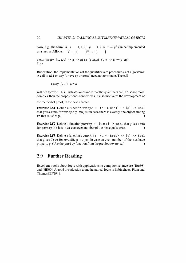
7/16/2019 The Haskell Road to Logic Maths and Programming
http://slidepdf.com/reader/full/the-haskell-road-to-logic-maths-and-programming-5634fa29ef7e9 81/448
70 CHAPTER 2. TALKING ABOUT MATHEMATICAL OBJECTS
Now, e.g., the formula
∀x
∈ 1, 4, 9
∃y
∈ 1, 2, 3
x = y2 can be implemented
as a test, as follows:
TAMO> every [1,4,9] (\ x -> some [1,2,3] (\ y -> x == y^2))
True
But caution: the implementations of the quantifiers are procedures, not algorithms.A call to all or any (or every or some) need not terminate. The call
every [0..] (>=0)
will run forever. This illustrates once more that the quantifiers are in essence more
complex than the propositional connectives. It also motivates the development of
the method of proof, in the next chapter.
Exercise 2.51 Define a function unique :: (a -> Bool) -> [a] -> Bool
that gives True for unique p xs just in case there is exactly one object among
xs that satisfies p.
Exercise 2.52 Define a function parity :: [Bool] -> Bool that gives True
for parity xs just in case an even number of the xss equals True.
Exercise 2.53 Define a function evenNR :: (a -> Bool) -> [a] -> Bool
that gives True for evenNR p xs just in case an even number of the xss have
property p. (Use the parity function from the previous exercise.)
2.9 Further Reading
Excellent books about logic with applications in computer science are [Bur98]
and [HR00]. A good introduction to mathematical logic is Ebbinghaus, Flum and
Thomas [EFT94].

7/16/2019 The Haskell Road to Logic Maths and Programming
http://slidepdf.com/reader/full/the-haskell-road-to-logic-maths-and-programming-5634fa29ef7e9 82/448
Chapter 3
The Use of Logic: Proof
Preview
This chapter describes how to write simple proofs. Section 3.1 is about style of
presentation, while Section 3.2 gives the general format of the proof rules. Sec-
tions 3.3 and 3.4 describe the rules that govern the use of the connectives and
the quantifiers in the proof process. The recipes are summarized in Section 3.5.
Section 3.6 gives some strategic hints for handling proof problems. Section 3.7
applies the proof recipes to reasoning about prime numbers; this section also illus-
trates how the computer can be used (sometimes) as an instrument for checking
particular cases, and therefore as a tool for refuting general claims.
Representation and proof are two sides of the same coin. In order to handle the
stuff of mathematics, we start out from definitions and try to find meaningful rela-
tions. To check our intuitions and sometimes just to make sure that our definitions
accomplish what we had in mind we have to provide proofs for our conjectures.
To handle abstract objects in an implementation we have to represent them in a
concrete way. Again, we have to check that the representation is faithful to the
original intention.
It turns out that proofs and implementations have many things in common. In the
first place, variables are a key ingredient in both. Variables are used to denote
members of certain sets. In our example proofs, we will used x, y for rational
numbers and real numbers, and m, n for integers. Similarly, the variables used in
the implementation of a definition range over certain sets, indicated by means of
typings for the variables.
71

7/16/2019 The Haskell Road to Logic Maths and Programming
http://slidepdf.com/reader/full/the-haskell-road-to-logic-maths-and-programming-5634fa29ef7e9 83/448
72 CHAPTER 3. THE USE OF LOGIC: PROOF
The main purpose of this chapter is to spur you on to develop good habits in setting
up mathematical proofs. Once acquired, these habits will help you in many ways.Being able to ‘see structure’ in a mathematical proof will enable you to easily read
and digest the proofs you find in papers and textbooks. When you have learned to
see the patterns of proof, you will discover that they turn up again and again in any
kind of formal reasoning.
Because it takes time to acquire new habits, it is not possible to digest the contents
of this chapter in one or two readings. Once the recommended habits are acquired,
but only then, the contents of the chapter have been properly digested, and the
chapter will have served its purpose.
The module containing the code of this chapter depends on the module containing
the code of the previous chapter. In the module declaration we take care to import
that module. This is done with the reserved keyword import.
module TUOLP
where
import TAMO
3.1 Proof Style
The objects of mathematics are strange creatures. They do not exist in physical
space. No one ever saw the number 1. One can consistently argue that mathematics
has no subject at all, or maybe that the subject matter of mathematics is in the
mind. But what does that mean? For sure, different mathematicians have the same
objects in mind when they investigate prime numbers. But how can that be, if
mathematics has no subject matter?
As to the method of mathematics, there is no disagreement: the heart of the matter
is the notion of proof . A proof is an argument aimed at convincing yourself and
others of the truth of an assertion. Some proofs are simple, but others can be pieces
of art with aesthetic and intellectual qualities.
In daily life, people argue a lot, but these efforts are not always capable of convinc-
ing others. If you have a row with your partner, more often than not it is extremely
difficult to assess who is right. (If this were an easy matter, why have a row in

7/16/2019 The Haskell Road to Logic Maths and Programming
http://slidepdf.com/reader/full/the-haskell-road-to-logic-maths-and-programming-5634fa29ef7e9 84/448
3.1. PROOF STYLE 73
the first place?) By contrast, in mathematical matters it usually is very clear who
is right and who is wrong. Doing mathematics is a sports where the rules of thegame are very clear. Indeed, mathematical proofs go undisputed most of the time.
This remarkable phenomenon is probably due to the idealized character of mathe-
matical objects. Idealization is a means by which mathematics provides access to
the essence of things, and grasping the essence of something is a hallmark of the
creative mind. It remains a source of wonder that the results are so often applicable
to the real world.
The mathematical content of most of the proofs discussed in this chapter is minute;
later on you will call such proofs “routine”. For the time being, the attention is
focused on the form of proofs. However, to begin with, here follows a list of
stylistic commandments.
A proof is made up of sentences. Therefore:
1 Write correct English, try to express yourself clearly.
If you are not a native speaker you are in the same league as the authors of this
book. Still, English is the lingua franca of the exact sciences, so there is no way
around learning enough of it for clear communication. Especially when not a
native speaker, keep your style simple.
Write with a reader in mind, and do not leave your reader in the dark concerning
your proof plans.
2 Make sure the reader knows exactly what you are up to.
Applying the rules of proof of the next section in the correct way will usually take
care of this. In particular, when you feel the need to start writing symbols —often,
variables— inform the reader what they stand for and do not let them fall out of
the blue.
3 Say what you mean when introducing a variable.
Section 3.2 again shows you the way.
Use the symbolic shorthands for connectives and quantifiers sparingly. Something
like the continuity definition on p. 66 with its impressive sequence of four quanti-
fiers is about the maximum a well-educated mathematician can digest.
4 Don’t start a sentence with symbols; don’t write formulas only.

7/16/2019 The Haskell Road to Logic Maths and Programming
http://slidepdf.com/reader/full/the-haskell-road-to-logic-maths-and-programming-5634fa29ef7e9 85/448
74 CHAPTER 3. THE USE OF LOGIC: PROOF
It is best to view symbolic expressions as objects in their own right. E.g., write:
The formula Φ is true, or: It holds that Φ. Note that a proof that consists of formulas only is not a suitable way to inform the reader about what has been going
on in your brain.
5 Use words or phrases like ‘thus’ , ‘therefore’ , ‘hence’ , ‘it follows that’ ,etc.
to link up your formulas. Be relevant and succinct.
Do not use the implication symbol ⇒ in cases that really require “thus” or “there-
fore”. Beginner’s proofs can often be recognized by their excessive length. Of
course, it will be difficult at first to keep to the proper middle road between com-
mandments (4) and (5).
When embarking on a proof, it is a good idea to write down exactly (i) what can
be used in the proof (the Given), (ii) and what is to be proved. It is very helpful to
use a schema for this.
6 When constructing proofs, use the following schema:
Given: . . .
To be proved: . . .
Proof: . . .
N.B.: A proof using Mathematical Induction offers some extra structure; cf. Sec-
tion 7.1 below and p. 400.
In the course of this chapter you will discover that proofs are highly structured
pieces of texts. The following guideline will help you keep track of that structure.
7 Use layout (in particular, indentation)to identify subproofs and to keep track
of the scopes of assumptions.
The general shape of a proof containing subproofs will be discussed in Section 3.2.
8 Look up definitions of defined notions, and use these definitions to re-write
both Given and To be proved.
In particular, elimination of defined notions from the sentence to be proved will
show you clearly what it is that you have to prove.
Do not expect that you will be able to write down a correct proof at the first try. Do
not expect to succeed at the second one. You will have to accept the fact that, for

7/16/2019 The Haskell Road to Logic Maths and Programming
http://slidepdf.com/reader/full/the-haskell-road-to-logic-maths-and-programming-5634fa29ef7e9 86/448
3.2. PROOF RECIPES 75
the time being, your efforts will not result in faultless proofs. Nevertheless: keep
trying!
9 Make sure you have a sufficient supply of scratch paper, make a fair copy of
the end-product — whether you think it to be flawless or not.
Finally: before handing in what you wrote, try to let it rest for at least one night.
And only then,
10 Ask yourself two things: Is this correct? Can others read it?
The honest answers usually will be negative at first.. . Fortunately, you did not
finish your supply of scratch paper. And surely, if you have understood properly,
you must be able to get it down correctly eventually. (Apply to this the law of
contraposition in Theorem 2.10, p. 45.)
3.2 Proof Recipes
Goal Develop the ability to apply the proof rules in simple contexts. The proof
rules are recipes that will allow you to cook up your own proofs. Try to distill
a recipe from every rule, and and make sure you remember how to apply theserecipes in the appropriate situation.
It is completely normal that you get stuck in your first efforts to prove things. Of-
ten, you will not even know how to make a first move. This section then may come
to your help. It provides you with rules that govern the behaviour of the logical
phrases in mathematical proof, and thus with recipes to use while constructing a
proof.
In fact, constructing proofs has a lot in common with writing computer programs.
In structured programming, layout can be used to reveal the building blocks of a
program more clearly. We will also use layout as a tool to reveal structure.
The most important structure principle is that a proof can contain subproofs, just
like a program may contain procedures which have their own sub-procedures, and
so on. We will indicate subproofs by means of indentation. The general structure
of a proof containing a subproof is as follows:

7/16/2019 The Haskell Road to Logic Maths and Programming
http://slidepdf.com/reader/full/the-haskell-road-to-logic-maths-and-programming-5634fa29ef7e9 87/448
76 CHAPTER 3. THE USE OF LOGIC: PROOF
Given: A, B, . . .
To be proved: P
Proof:
. . .
Suppose C . . .
To be proved: Q
Proof: . . .
. . .
Thus Q
. . .
Thus P
To be sure, a subproof may itself contain subproofs:
Given: A, B
To be proved: P
Proof:
. . .
Suppose C
To be proved: QProof:
. . .
Suppose D
To be proved: R
Proof: . . .
. . .
Thus R
. . .
Thus Q
. . .
Thus P
7/16/2019 The Haskell Road to Logic Maths and Programming
http://slidepdf.com/reader/full/the-haskell-road-to-logic-maths-and-programming-5634fa29ef7e9 88/448
3.2. PROOF RECIPES 77
The purpose of ‘Suppose’ is to add a new given to the list of assumptions that
may be used, but only for the duration of the subproof of which ‘Suppose’ is thehead. If the current list of givens is P 1, . . . , P n then ‘Suppose Q’ extends this list to
P 1, . . . , P n, Q. In general, inside a box, you can use all the givens and assumptions
of all the including boxes. Thus, in the innermost box of the example, the givens
are A ,B,C,D. This illustrates the importance of indentation for keeping track of
the ‘current box’.
There are some 15 rules discussed here for all seven notions of logic. At a first
encounter, this may seem an overwhelming number. However, only some of these
are really enlightening; several are so trivial that you won’t even notice using them.
An example is:
Given: P , Q
Thus P ∧ Q.
What is really remarkable is this: together these 15 rules are sufficient to tackle
every possible proof problem.
Of course, this does not mean that the process of proving mathematical facts boils
down in the end to mastery of a few simple rules. Think of it as chess: the rules of
the game are extremely simple, and these rules can be used to play very compli-
cated and beautiful games. To be able to play you must know the rules. But if your
knowledge does not extend beyond the rules, you will only be capable of playing
games that are rather dull. Learning to play chess does not stop with learning the
rules, and what is beautiful in a game of chess cannot be found in the rules. Sim-
ilarly, the rules of proof cannot teach you more than how to prove the simplest of
things. (And, in the beginning, that is difficult enough.) It is ideas that make aproof interesting or beautiful, but the rules keep silent about these things.
Classification of Rules.
Every logical symbol has its own rules of use. There are basically two ways in
which you can encounter a logical symbol: it can either appear in the given or in the
statement that is to be proved. In the first case the rule to use is an elimination rule,
in the second case an introduction rule. Elimination rules enable you to reduce a
proof problem to a new, hopefully simpler, one. Introduction rules make clear how
to prove a goal of a certain given shape. All rules are summarized in Section 3.5.
Safety. As we go along, we will provide arguments that try to explain why a
certain rule is safe. A rule is safe if it will never allow you to prove something
false on the basis of statements that are true. Obviously, this is a requirement that

7/16/2019 The Haskell Road to Logic Maths and Programming
http://slidepdf.com/reader/full/the-haskell-road-to-logic-maths-and-programming-5634fa29ef7e9 89/448
78 CHAPTER 3. THE USE OF LOGIC: PROOF
proofs should fulfill. That the rules for connectives are safe is due to truth tables.
Safety of two of the quantifier rules is obvious; the remaining ones are tough nuts.
Don’tworry when these explanations in some cases appear mystifying. Eventually,
you’ll understand!
3.3 Rules for the Connectives
Implication
Here come a complicated but important introduction rule and a trivial one for elim-
ination.
Introduction The introduction rule for implication is the Deduction Rule. It en-
ables you to reduce the problem of proving an implication Φ ⇒ Ψ. Instead, it
prescribes to assume Φ as an additional new Given, and asks you to derive that Ψ.
Given: . . .
To be proved: Φ ⇒ ΨProof:
Suppose ΦTo be proved: ΨProof: . . .
Thus Φ ⇒ Ψ.
Safety. In case Φ is false, the implication Φ ⇒ Ψ will be true anyway. Thus, the
case that is left for you to consider is when Φ is true, meaning that you can assume
it as given. But then of course you should show that Ψ is true as well (otherwise,
Φ ⇒ Ψ would be false).
Example 3.1 We show that the implication P ⇒ R is provable on the basis of the
given P ⇒ Q and Q ⇒ R. Thus, employing the schema in the 7th commandment
(p. 74) for the first time:
Given: P ⇒ Q, Q ⇒ RTo be proved: P ⇒ RProof:
Given: P ⇒ Q, Q ⇒ R (old), P (new)
To be proved: R
7/16/2019 The Haskell Road to Logic Maths and Programming
http://slidepdf.com/reader/full/the-haskell-road-to-logic-maths-and-programming-5634fa29ef7e9 90/448
3.3. RULES FOR THE CONNECTIVES 79
Proof: From P
⇒Q and P , conclude Q.
Next, from Q ⇒ R and Q, conclude R.
Thus, according to the deduction rule, P ⇒ R
Here is a slightly more concise version:
Given: P ⇒ Q, Q ⇒ RTo be proved: P ⇒ RProof:
Suppose P To be proved: RProof: From P ⇒ Q and P , conclude Q.
Next, from Q ⇒ R and Q, conclude R.
Thus P ⇒ R
Detailed vs. Concise Proofs. The proof just given explains painstakingly how the
Deduction Rule has been applied in order to get the required result. However, in
practice, you should write this in a still more concise way:
Given: P ⇒ Q, Q ⇒ RTo be proved: P ⇒ RProof:
Suppose P From P
⇒Q and P , conclude Q.
Next, from Q ⇒ R and Q, conclude R.
Note that the final concise version does not mention the Deduction Rule at all.
The actual application of this rule should follow as a last line, but that is left for
the reader to fill in. This is not considered an incomplete proof: from the situation
it is perfectly clear that this application is understood.
Several other examples of detailed proofs and their concise versions are given in
what follows. Here is the key to the proof of an implication:
If the ‘to be proved’ is an implication Φ ⇒ Ψ, then your proof should start with the
following Obligatory Sentence:
Suppose that Φ holds.

7/16/2019 The Haskell Road to Logic Maths and Programming
http://slidepdf.com/reader/full/the-haskell-road-to-logic-maths-and-programming-5634fa29ef7e9 91/448
80 CHAPTER 3. THE USE OF LOGIC: PROOF
The obligatory first sentence accomplishes the following things (cf. the 2nd com-
mandment on p. 73).
• It informs the reader that you are going to apply the Deduction Rule in order
to establish that Φ ⇒ Ψ.
• The reader also understands that it is now Ψ that you are going to derive
(instead of Φ ⇒ Ψ).
• Thus, starting with the obligatory sentence informs the reader in an efficient
way about your plans.
Reductive Character. In Example (3.1) the problem of showing that from the
givens P
⇒Q, Q
⇒R it can be proved that P
⇒R was reduced , using the
Deduction Rule, to the problem of showing that from the givens P ⇒ Q, Q ⇒R, P it can be proved that R. This requires a subproof.
Marking Subproofs with Indentation. Note that only during that subproof you
are allowed to use the new given P . Some logic texts recommend the use of
markers to indicate beginning and end of such a subproof, between which the
extra given is available. In our example proofs in this chapter, we indicate the
beginnings and ends of subproofs by means of indentation. In more colloquial
versions of the proofs, identifying the beginning and end of a subproof is left to
the reader.
In this particular case, the reduced proof problem turned out to be easy: P and
P ⇒ Q together produce Q; whereas Q and Q ⇒ R together produce R, asdesired. (Of course, in general, such a subproof may require new reductions.)
The last two steps in this argument in fact apply the Elimination Rule of implica-
tion, which is almost too self-evident to write down:
Elimination. This rule is also called Modus Ponens. In words: from Φ ⇒ Ψ and
Φ you can conclude that Ψ.
In a schema:
Given: Φ ⇒ Ψ, ΦThus Ψ.
Safety. Immediate from truth tables: if Φ ⇒ Ψ and Φ are both true, then so is Ψ.

7/16/2019 The Haskell Road to Logic Maths and Programming
http://slidepdf.com/reader/full/the-haskell-road-to-logic-maths-and-programming-5634fa29ef7e9 92/448
3.3. RULES FOR THE CONNECTIVES 81
The two proof rules for implication enable you to handle implications in all types
of proof problems. You may want to use more obvious properties of implication,but fact is that they usually can be derived from the two given ones. Example (3.1)
is a case in point, as is Exercise 3.2. (We will not bother you with the exceptions;
one is in Exercise 3.9.)
Exercise 3.2 Apply both implication rules to prove P ⇒ R from the givens P ⇒Q, P ⇒ (Q ⇒ R).
Conjunction
The conjunction rules are almost too obvious to write down.
Introduction. A conjunction follows from its two conjuncts taken together.
In a schema:
Given: Φ, ΨThus Φ ∧ Ψ.
Elimination. From a conjunction, both conjuncts can be concluded.
Schematically:
Given: Φ ∧ Ψ
Thus Φ.
Given: Φ ∧ ΨThus Ψ.
Suppose we want to check whether the sum of even natural numbers always is
even. It is not difficult to implement this check in Haskell, using the built-in func-
tion even and the list of even numbers.
evens = [ x | x <- [0..], even x ]
Formulating the check is easy, but of course we won’t get an answer, as the check
takes an infinite amount of time to compute.
7/16/2019 The Haskell Road to Logic Maths and Programming
http://slidepdf.com/reader/full/the-haskell-road-to-logic-maths-and-programming-5634fa29ef7e9 93/448
82 CHAPTER 3. THE USE OF LOGIC: PROOF
TUOLP> forall [ m + n | m <- evens, n <- evens ] even
If we want to check a statement about an infinite number of cases, we can either
look for a counterexample, or we can attempt to give a proof. In the present case,
the latter is easy.
Example 3.3 Assume that n, m ∈ N.
To show: (m is even ∧ n is even) ⇒ m + n is even.
Detailed proof:
Assume that (m even ∧ n even).
Then (∧-elimination) m and n are both even.
For instance, p, q ∈N exist such that m = 2 p, n = 2q .
Then m + n = 2 p + 2q = 2( p + q ) is even.
The result follows using the Deduction Rule.
Concise proof:
Assume that m and n are even.
For instance, m = 2 p, n = 2q , p, q ∈ N.
Then m + n = 2 p + 2q = 2( p + q ) is even.
Exercise 3.4 Assume that n, m ∈ N.
Show: (m is odd ∧ n is odd) ⇒ m + n is even.
Equivalence
An equivalence can be thought of as the conjunction of two implications. Thus,
the rules follow from those for ⇒ and ∧.
Introduction. In order to prove Φ ⇔ Ψ, you have to accomplish two things (cf.
example 2.3):
(⇒) add Φ as a new given, and show that Ψ;
(
⇐) add Ψ as a new given, and show that Φ.
If you can do this, Φ ⇔ Ψ has been proved.

7/16/2019 The Haskell Road to Logic Maths and Programming
http://slidepdf.com/reader/full/the-haskell-road-to-logic-maths-and-programming-5634fa29ef7e9 94/448
3.3. RULES FOR THE CONNECTIVES 83
Concise Proof Schema.
Given: . . .
To be proved: Φ ⇔ ΨProof:
Suppose ΦTo be proved: ΨProof: . . .
Suppose ΨTo be proved: ΦProof: . . .
Thus Φ ⇔ Ψ.
Instead of ⇔ youmay also encounter ‘iff’or ‘if and only if’. A proofof a statement
of the form ‘Φ iff Ψ’ consists of two subproofs: the proof of the ‘only if’ part and
the proof of the ‘if’ part. Caution: the ‘only if’ part is the proof of Φ ⇒ Ψ, and
the ‘if’ part is the proof of Φ ⇐ Ψ. This is because ‘Φ only if Ψ’ means ‘Φ ⇒ Ψ’,
and ‘Φ if Ψ’ means ‘Φ ⇐ Ψ’. Thus, we get:
Given: . . .
To be proved: Φ iff ΨProof:
Only if: Suppose ΦTo be proved: ΨProof: . . .
If: Suppose ΨTo be proved: ΦProof: . . .
Thus Φ iff Ψ.
Elimination. Schematically:
Given: Φ ⇔ Ψ, Φ, . . .
Thus Ψ
Given: Φ ⇔ Ψ, Ψ, . . .
Thus Φ
Exercise 3.5 Show:

7/16/2019 The Haskell Road to Logic Maths and Programming
http://slidepdf.com/reader/full/the-haskell-road-to-logic-maths-and-programming-5634fa29ef7e9 95/448
84 CHAPTER 3. THE USE OF LOGIC: PROOF
1. From P
⇔Q it follows that (P
⇒R)
⇔(Q
⇒R),
2. From P ⇔ Q it follows that (R ⇒ P ) ⇔ (R ⇒ Q).
Negation
General Advice. In no matter what concrete mathematical situation, before ap-
plying any of the negation rules given below: whether you want to prove or use
a negated sentence, you should first attempt to convert into something positive. If
this succeeds, you can turn to the other rules.
Theorems 2.10 (p. 45) and 2.40 (p. 65) contain some tools for doing this: you canmove the negation symbol inward, across quantifiers and connectives. If this pro-
cess terminates, the “mathematics” of the situation often allows you to eliminate
the negation symbol altogether. E.g., ¬∀x(x < a ∨ b x) can be rewritten as
∃x(a x ∧ x < b). For a more complicated example, cf. (2.49) on p. 67.
Remark. The general advice given above does not apply to the exercises in the
present chapter. Firstly, many of the exercises below are purely logical: there is
no mathematical context at all. Secondly, all exercises here are designed to be
solved using the rules only; possible shortcuts via the results of Chapter 2 will
often trivialize them.
Introduction. If ¬Φ is to be proved, do the following. Assume Φ as a new given,and attempt to prove something (depending on the context) that is evidently false.
This strategy clearly belongs to the kind of rule that reduces the proof problem.
Schematically:
Given: . . .
To be proved: ¬ΦProof:
Suppose ΦTo be proved: ⊥Proof: . . .
Thus
¬Φ.
Evidently False. Here, ⊥ stands for the evidently false statement.

7/16/2019 The Haskell Road to Logic Maths and Programming
http://slidepdf.com/reader/full/the-haskell-road-to-logic-maths-and-programming-5634fa29ef7e9 96/448
3.3. RULES FOR THE CONNECTIVES 85
In a mathematical context, this can be anything untrue, such as 1 = 0. For a more
complicated falsehood, cf. the proof that limits are unique on p. 317.
In the logical examples below, ⊥ may consist of the occurrence of a statement
together with its negation. In that case, one statement contradicts the other. For
instance, you might derive a sentence ¬Ψ, thereby contradicting the occurrence of
Ψ among the given Γ. Cf. Examples (3.8) and and (3.30).
Example 3.6 The proof of theorem 3.33 (the number of primes is not finite) is an
example of the method of negation introduction. Another example can be found in
the proof of theorem 8.14 (the square root of 2 is not rational).
Exercise 3.7 Produce proofs for:
1. Given: P ⇒ Q. To show: ¬Q ⇒ ¬P ,
2. Given P ⇔ Q. To show: ¬P ⇔ ¬Q.
Safety. Suppose that from Γ, Φ it follows that ⊥, and that all given Γ are satisfied.
Then Φ cannot be true. (Otherwise, your proof would show the evidently false ⊥to be true as well.) Thus, ¬Φ must be true.
Elimination. When you intend to use the given ¬Φ, you can attempt to prove,
on the basis of the other given, that Φ must hold. In that case, the eliminationrule declares the proof problem to be solved, no matter what the statement To be
proved!
Schematically:
Given: Φ, ¬ΦThus Ψ.
Safety. The rule cannot help to be safe, since you will never find yourself in a
situation where Φ and ¬Φ are both true. (Remarkably, this nevertheless is a useful
rule!)
There is one extra negation rule that can be used in every situation: Proof by
Contradiction, or Reductio ad Absurdum.

7/16/2019 The Haskell Road to Logic Maths and Programming
http://slidepdf.com/reader/full/the-haskell-road-to-logic-maths-and-programming-5634fa29ef7e9 97/448
86 CHAPTER 3. THE USE OF LOGIC: PROOF
Proof by Contradiction. In order to prove Φ, add
¬Φ as a new given, and attempt
to deduce an evidently false statement.
In a schema:
Given: . . .
To be proved: ΦProof:
Suppose ¬ΦTo be proved: ⊥Proof: . . .
Thus Φ.
Safety. The argument is similar to that of the introduction rule.
Advice. Beginners are often lured into using this rule. The given ¬Φ that comes
in free looks so inviting! However, many times it must be considered poisoned,
making for a cluttered bunch of confused givens that you will not be able to disen-
tangle. It is a killer rule that often will turn itself against its user, especially when
that is a beginner. Proof by Contradiction should be considered your last way out.
Some proof problems do need it, but if possible you should proceed without: you
won’t get hurt and a simpler and more informative proof will result.
Comparison. Proof by Contradiction looks very similar to the ¬ introduction rule
(both in form and in spirit), and the two are often confused. Indeed, in ordinary
mathematical contexts, it is usually “better” to move negation inside instead of
applying ¬-introduction.
Example 3.8 From ¬Q ⇒ ¬P it follows that P ⇒ Q.
Given: ¬Q ⇒ ¬P To be proved: P ⇒ QDetailed proof:
Suppose P To be proved: QProof:
Suppose ¬QTo be proved: ⊥Proof:
From ¬Q and ¬Q ⇒ ¬P derive ¬P .From P and ¬P derive ⊥.

7/16/2019 The Haskell Road to Logic Maths and Programming
http://slidepdf.com/reader/full/the-haskell-road-to-logic-maths-and-programming-5634fa29ef7e9 98/448
3.3. RULES FOR THE CONNECTIVES 87
Thus, Q, by contradiction.
Thus, P ⇒ Q, by the Deduction Rule.
Concise proof:
Assume that P .If ¬Q, then (by ¬Q ⇒ ¬P ) it follows that ¬P .Contradiction.
Exercise 3.9* Show that from (P ⇒ Q) ⇒ P it follows that P .
Hint. Apply Proof by Contradiction. (The implication rules do not suffice for this
admittedly exotic example.)
Disjunction
Introduction. A disjunction follows from each of its disjuncts.
Schematically:
Given: ΦThus Φ ∨ Ψ.
Given: ΨThus Φ ∨ Ψ.
Safety is immediate from the truth tables.
Elimination. You can use a given Φ ∨ Ψ by giving two proofs: one employing
Φ, and one employing Ψ.
In a proof schema:
Given: Φ ∨ Ψ, . . .
To be proved: ΛProof:
Suppose ΦTo be proved: ΛProof: . . .
Suppose ΨTo be proved: Λ

7/16/2019 The Haskell Road to Logic Maths and Programming
http://slidepdf.com/reader/full/the-haskell-road-to-logic-maths-and-programming-5634fa29ef7e9 99/448
88 CHAPTER 3. THE USE OF LOGIC: PROOF
Proof: . . .
Thus Λ.
Example 3.10 We show that from P ∨ Q, ¬P it follows that Q.
Given: P ∨ Q, ¬P .To be proved: Q.
Proof:
Suppose P . Then from P and ¬P we get Q.
Suppose Q. Then Q holds by assumption.
Therefore Q.
Exercise 3.11 Assume that A ,B,C and D are statements.
1. From the given A ⇒ B ∨ C and B ⇒ ¬A, derive that A ⇒ C . (Hint: use
the previous example.)
2. From the given A ∨ B ⇒ C ∨ D, C ⇒ A, and B ⇒ ¬A, derive that
B ⇒ D.
Example 3.12 Here is a proof of the second DeMorgan law (Theorem 2.10):
Given: ¬(P ∨ Q).
To be proved: ¬P ∧ ¬Q.
Detailed proof:
Assume P . By ∨ -introduction, it follows that P ∨ Q.
This contradicts the given (i.e., we have an evident falsity here).
By ¬-introduction, we get ¬P .In a similar way, ¬Q can be derived.
By ∧-introduction, it follows that ¬P ∧ ¬Q.
The concise version (no rules mentioned):
Assume P . Then a fortiori P ∨ Q holds, contradicting the given.
Thus, ¬P . Similarly, ¬Q is derivable.
Thus,
¬P
∧ ¬Q follows.

7/16/2019 The Haskell Road to Logic Maths and Programming
http://slidepdf.com/reader/full/the-haskell-road-to-logic-maths-and-programming-5634fa29ef7e9 100/448
3.3. RULES FOR THE CONNECTIVES 89
Example 3.13 The following example from the list of equivalences in Theorem
(2.10) is so strange that we give it just to prevent you from getting entangled.
Given: ¬(P ⇒ Q)To be proved: P ∧ ¬QProof: By ∧-introduction, it suffices to prove both P and ¬Q.
To be proved: P Proof: (by contradiction)
Suppose that ¬P .Then if P holds, Q follows by ¬-elimination.
Thus (Deduction Rule), we get that P ⇒ Q.
However, this contradicts the given.
To be proved:
¬Q
Proof: (by ¬ introduction)Assume that Q.
Then, by a trivial application of the Deduction Rule P ⇒ Q follows.
(Trivial, since we do not need P at all to conclude Q.)
Again, this contradicts the given.
Note that the rule for implication introduction can be used for reasoning by cases,
as follows. Because P ∨ ¬P is a logical truth, it can always be added to the list of
givens. If the two sub cases P and ¬P both yield conclusion Q, then this proves
Q. Here is the schema:
Given: . . .
To be proved: QProof:
Suppose P .To be proved: Q.
Proof: . . .
Suppose ¬P .To be proved: Q.
Proof: . . .
Thus Q.
This pattern of reasoning is used in the following examples.
Example 3.14

7/16/2019 The Haskell Road to Logic Maths and Programming
http://slidepdf.com/reader/full/the-haskell-road-to-logic-maths-and-programming-5634fa29ef7e9 101/448
90 CHAPTER 3. THE USE OF LOGIC: PROOF
Let n
∈N. To be proved: n2
−n is even.
Proof:Assume n even.
Then n = 2m, so n2 − n = (n − 1)n = (2m − 1)2m,
and therefore n2 − n is even.
Assume n odd.
Then n = 2m + 1, so n2 − n = (n − 1)n = 2m(2m + 1),
and therefore n2 − n is even.
Thus n2 − n is even.
Exercise 3.15 Show that for any n ∈ N, division of n2 by 4 gives remainder 0 or
1.
Example 3.16 Let R be the universe of discourse, and let P (x) be the following
property:
x /∈ Q ∧ x√
2 ∈ Q.
In other words, x has property P iff x is irrational and x√
2 is rational. We will
show that either√
2 or√
2√ 2 has property P .
Suppose√
2√ 2 ∈ Q.
Then, since√
2 /∈ Q (Theorem 8.14), we know that√
2 has P .Thus, P (
√ 2) ∨ P (
√ 2√ 2).
Suppose√
2√ 2 /∈ Q.
Then, since (
√ 2√ 2
)
√ 2
=
√ 2√ 2·√ 2
=
√ 2
2
= 2 ∈Q
, we know that
√ 2√ 2
has P .Thus, P (√
2) ∨ P (√
2√ 2).
Therefore P (√
2) ∨ P (√
2√ 2).
Exercise 3.17 Prove the remaining items of Theorem 2.10 (p. 45). To prove Φ ≡Ψ means (i) to derive Ψ from the given Φ and (ii) to derive Φ from the given Ψ.
3.4 Rules for the Quantifiers
The rules for the quantifiers come in two types: for the unrestricted, and for the
restricted versions. Those for the restricted quantifiers can be derived from the
others: see Exercise 3.32 p. 102.

7/16/2019 The Haskell Road to Logic Maths and Programming
http://slidepdf.com/reader/full/the-haskell-road-to-logic-maths-and-programming-5634fa29ef7e9 102/448
3.4. RULES FOR THE QUANTIFIERS 91
Universal Quantifier
Introduction.
When asked to prove that ∀x E (x), you should start a proof by writing the Obligatory
Sentence:
Suppose that c is an arbitrary object.
And you proceed to show that this object (about which you are not supposed toassume extra information; in particular, it should not occur earlier in the argument)
has the property E in question.
Schematic form:
Given: . . .
To be proved: ∀xE (x)Proof:
Suppose c is an arbitrary object
To be proved: E (c)Proof: . . .
Thus
∀xE (x)
Here is the Modification suitable for the restricted universal quantifier:
If ∀x ∈ A E (x) is to be proved, you should start proof this time by the, again, obliga-
tory:
Suppose that c is any object in A.
And you proceed to show that this object (about which you only assume that it
belongs to A) has the property E in question.
Schematic form:
7/16/2019 The Haskell Road to Logic Maths and Programming
http://slidepdf.com/reader/full/the-haskell-road-to-logic-maths-and-programming-5634fa29ef7e9 103/448
92 CHAPTER 3. THE USE OF LOGIC: PROOF
Given: . . .
To be proved: ∀x ∈ A E (x)Proof:
Suppose c is any object in ATo be proved: E (c)Proof: . . .
Thus ∀x ∈ A E (x)
Arbitrary Objects. You may wonder what an arbitrary object is. For instance:
what is an arbitrary natural number? Is it large? small? prime? etc. What exactly
is an arbitrary object in A when this set happens to be a singleton? And: are there
objects that are not arbitrary?
Answer: the term ‘arbitrary object’ is only used here as an aid to the imagination;
it indicates something unspecified about which no special assumptions are made.
Imagine that you allow someone else to pick an object, and that you don’t care
what choice is made. ‘Suppose c is an arbitrary A’ is the same as saying to the
reader: ‘Suppose you provide me with a member c from the set A; the choice is
completely up to you.’
Often, a universal quantifier occurs in front of an implication. Therefore, you may
find the following rule schema useful.
Given: . . .
To be proved: ∀x(P (x) ⇒ Q(x)Proof:
Suppose c is any object such that P (c)To be proved: Q(c)Proof: . . .
Thus ∀x(P (x) ⇒ Q(x))
This rule is derivable from the introduction rules for ∀ and ⇒. Note that it is very
similar to the recipe for restricted ∀-introduction. Cf. Exercise 3.18.
Elimination.
Schematic form:
Given:
∀x E (x)
Thus E (t).
Here, t is any object of your choice.

7/16/2019 The Haskell Road to Logic Maths and Programming
http://slidepdf.com/reader/full/the-haskell-road-to-logic-maths-and-programming-5634fa29ef7e9 104/448
3.4. RULES FOR THE QUANTIFIERS 93
That this rule is safe is obvious: if every thing satisfies E , then in particular so
must t.
Modification suitable for the restricted universal quantifier, in schematic form:
Given: ∀x ∈ A E (x), t ∈ AThus E (t).
Exercise 3.18 Show, using ∀-introduction and Deduction Rule: if from Γ, P (c) it
follows that Q(c) (where c satisfies P , but is otherwise “arbitrary”), then from Γ it
follows that ∀x(P (x) ⇒ Q(x)).
Existential Quantifier
Introduction. In order to show that ∃x E (x), it suffices to specify one object t forwhich E (t) holds.
Schematic form:
Given: E (t)Thus, ∃x E (x).
Here, t can be anything: any example satisfying E can be used to show that
∃xE (x).
Modification suitable for the restricted existential quantifier, in schematic form:
Given: E (t), t ∈ AThus, ∃x ∈ A E (x).
That these rules are safe goes without saying.
Example-objects. An object t such that E (t) holds is an example-object for E .Thus, the introduction rule concludes ∃xE (x) from the existence of an example-
object.
However, it is not always possible or feasible to prove an existential statement by
exhibiting a specific example-object, and there are (famous) proofs of existential
statements that do not use this rule.
Example 3.19 A transcendent real is a real which is not a root of a polynomial
with integer coefficients (a polynomial f (x) = anxn+an−1xn−1 +. . .+a1x+a0,
where the ai are integers and an
= 0).
By an argument establishing that the set of reals must be strictly larger than the
set of roots of polynomials with integer coefficients, it is relatively easy to show
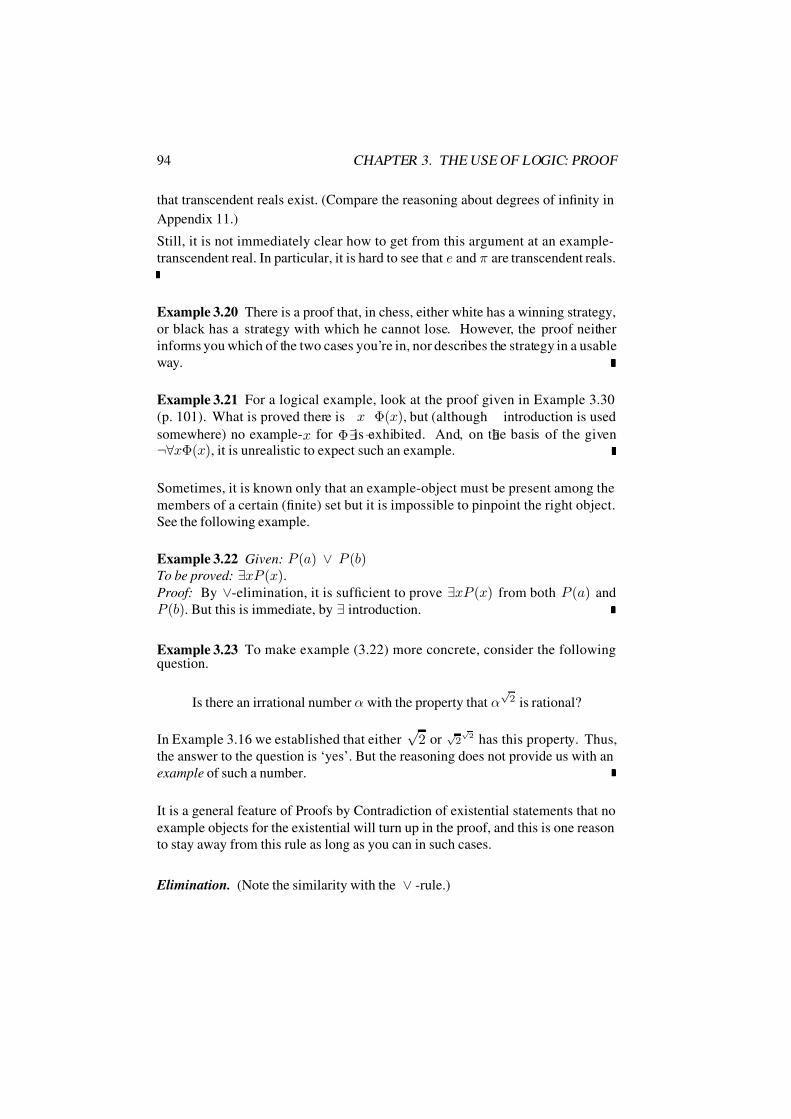
7/16/2019 The Haskell Road to Logic Maths and Programming
http://slidepdf.com/reader/full/the-haskell-road-to-logic-maths-and-programming-5634fa29ef7e9 105/448
94 CHAPTER 3. THE USE OF LOGIC: PROOF
that transcendent reals exist. (Compare the reasoning about degrees of infinity in
Appendix 11.)
Still, it is not immediately clear how to get from this argument at an example-
transcendent real. In particular, it is hard to see that e and π are transcendent reals.
Example 3.20 There is a proof that, in chess, either white has a winning strategy,
or black has a strategy with which he cannot lose. However, the proof neither
informs you which of the two cases you’re in, nor describes the strategy in a usable
way.
Example 3.21 For a logical example, look at the proof given in Example 3.30
(p. 101). What is proved there is
∃x
¬Φ(x), but (although
∃introduction is used
somewhere) no example-x for Φ is exhibited. And, on the basis of the given
¬∀xΦ(x), it is unrealistic to expect such an example.
Sometimes, it is known only that an example-object must be present among the
members of a certain (finite) set but it is impossible to pinpoint the right object.
See the following example.
Example 3.22 Given: P (a) ∨ P (b)To be proved: ∃xP (x).
Proof: By ∨-elimination, it is sufficient to prove ∃xP (x) from both P (a) and
P (b). But this is immediate, by ∃ introduction.
Example 3.23 To make example (3.22) more concrete, consider the followingquestion.
Is there an irrational number α with the property that α√
2 is rational?
In Example 3.16 we established that either√
2 or√
2√ 2 has this property. Thus,
the answer to the question is ‘yes’. But the reasoning does not provide us with an
example of such a number.
It is a general feature of Proofs by Contradiction of existential statements that no
example objects for the existential will turn up in the proof, and this is one reason
to stay away from this rule as long as you can in such cases.
Elimination. (Note the similarity with the ∨ -rule.)
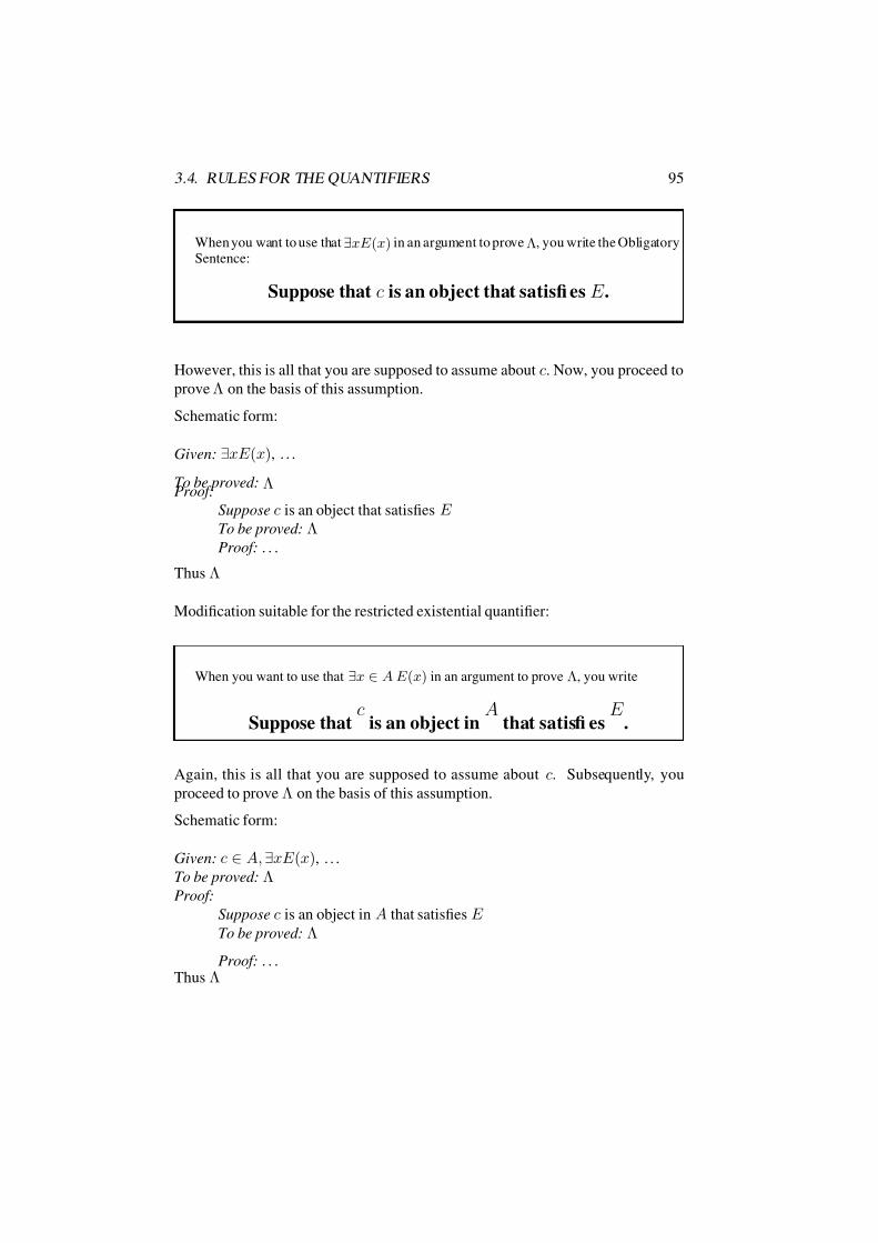
7/16/2019 The Haskell Road to Logic Maths and Programming
http://slidepdf.com/reader/full/the-haskell-road-to-logic-maths-and-programming-5634fa29ef7e9 106/448
3.4. RULES FOR THE QUANTIFIERS 95
When you want to use that ∃xE (x) in an argument to prove Λ, you write the Obligatory
Sentence:
Suppose that c is an object that satisfi es E .
However, this is all that you are supposed to assume about c. Now, you proceed to
prove Λ on the basis of this assumption.
Schematic form:
Given: ∃xE (x), . . .
To be proved: ΛProof:
Suppose c is an object that satisfies E To be proved: ΛProof: . . .
Thus Λ
Modification suitable for the restricted existential quantifier:
When you want to use that ∃x ∈ A E (x) in an argument to prove Λ, you write
Suppose thatc
is an object inA
that satisfi esE
.
Again, this is all that you are supposed to assume about c. Subsequently, you
proceed to prove Λ on the basis of this assumption.
Schematic form:
Given: c ∈ A, ∃xE (x), . . .
To be proved: ΛProof:
Suppose c is an object in A that satisfies E To be proved: Λ
Proof: . . .Thus Λ
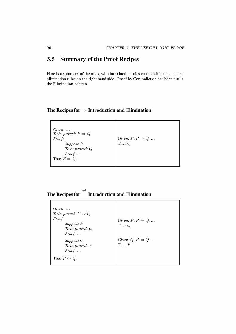
7/16/2019 The Haskell Road to Logic Maths and Programming
http://slidepdf.com/reader/full/the-haskell-road-to-logic-maths-and-programming-5634fa29ef7e9 107/448
96 CHAPTER 3. THE USE OF LOGIC: PROOF
3.5 Summary of the Proof Recipes
Here is a summary of the rules, with introduction rules on the left hand side, and
elimination rules on the right hand side. Proof by Contradiction has been put in
the Elimination-column.
The Recipes for ⇒ Introduction and Elimination
Given: . . .To be proved: P ⇒ QProof:
Suppose P To be proved: QProof: . . .
Thus P ⇒ Q.
Given: P , P ⇒ Q, . . .
Thus Q
The Recipes for⇔
Introduction and Elimination
Given: . . .
To be proved: P ⇔ QProof:
Suppose P To be proved: QProof: . . .
Suppose QTo be proved: P Proof: . . .
Thus P ⇔ Q.
Given: P , P ⇔ Q, . . .
Thus Q
Given: Q, P ⇔ Q, . . .
Thus P

7/16/2019 The Haskell Road to Logic Maths and Programming
http://slidepdf.com/reader/full/the-haskell-road-to-logic-maths-and-programming-5634fa29ef7e9 108/448
3.5. SUMMARY OF THE PROOF RECIPES 97
The Recipes for ¬ Introduction and Elimination
Given: . . .
To be proved: ¬P Proof:
Suppose P To be proved: ⊥Proof: . . .
Thus ¬P .
Given: . . .
To be proved: P Proof:
Suppose ¬P To be proved: ⊥Proof: . . .
Thus P .
Given: P , ¬P Thus Q.
The Recipes for ∧ Introduction and Elimination
Given: P , QThus P ∧ Q.
Given: P ∧ QThus P .
Given: P ∧ QThus Q.
The Recipes for ∨ Introduction and Elimination
Given: P Thus P ∨ Q.
Given: QThus P ∨ Q.
Given: P ∨ Q, . . .
To be proved: RProof:
Suppose P To be proved: RProof: . . .
Suppose QTo be proved: RProof: . . .
Thus R.

7/16/2019 The Haskell Road to Logic Maths and Programming
http://slidepdf.com/reader/full/the-haskell-road-to-logic-maths-and-programming-5634fa29ef7e9 109/448
98 CHAPTER 3. THE USE OF LOGIC: PROOF
The Recipes for ∀ Introduction and Elimination
Given: . . .
To be proved: ∀xE (x)Proof:
Suppose c is an arbitrary object
To be proved: E (c)Proof: . . .
Thus ∀xE (x)
Given: ∀xE (x), . . .
Thus E (t).
Given: . . .
To be proved: ∀x ∈ A E (x)Proof:
Suppose c is any object in ATo be proved: E (c)Proof: . . .
Thus ∀x ∈ A E (x)
Given: ∀x ∈ A E (x), t ∈ A, . . .
Thus E (t).
The Recipes for ∃ Introduction and Elimination
Given: E (t), . . .
Thus ∃xE (x).
Given: ∃xE (x), . . .
To be proved: P Proof:
Suppose c is an object that satisfies E To be proved: P Proof: . . .
Thus P

7/16/2019 The Haskell Road to Logic Maths and Programming
http://slidepdf.com/reader/full/the-haskell-road-to-logic-maths-and-programming-5634fa29ef7e9 110/448
3.6. SOME STRATEGIC GUIDELINES 99
Given: t ∈ A, E (t), . . .
Thus ∃x ∈ A E (x).
Given: ∃x ∈ A E (x), . . .To be proved: P Proof:
Suppose c is an object in A that satisfies E To be proved: P Proof: . . .
Thus P
3.6 Some Strategic Guidelines
Here are the most important guidelines that enable you to solve a proof problem.
1. Do not concentrate on the given, by trying to transform that into what is to
be proved.
2. Instead, concentrate on (the form of) what is to be proved.
3. A number of rules enable you to simplify the proof problem. For instance:
• When asked to prove P ⇒ Q, add P to the givens and try to prove Q.
(Deduction Rule).
• When asked to prove ∀x E (x), prove E (c) for an arbitrary c instead
(∀-introduction).
4. Only after you have reduced the problem as far as possible you should look
at the givens in order to see which of them can be used.
• When one of the givens is of the form P ∨ Q, and R is to be proved,
make a case distinction: first add P to the givens and prove R, next
add Q to the givens and prove R.
• When one of the givens is of the form ∃x E (x), and P is to be proved,
give the object that satisfies E a name, by adding E (c) to the givens.
Next, prove P .
5. It is usually a good idea to move negations inward as much as possible before
attempting to apply¬
-introduction.
6. Stay away from Proof by Contradiction as long as possible.
7/16/2019 The Haskell Road to Logic Maths and Programming
http://slidepdf.com/reader/full/the-haskell-road-to-logic-maths-and-programming-5634fa29ef7e9 111/448
100 CHAPTER 3. THE USE OF LOGIC: PROOF
Example 3.24 To show: from
∀x(P (x)
⇒Q(x)),
∃xP (x) it follows that
∃xQ(x).
Concise proof: Using the second given, assume that x is such that P (x) holds.
Applying the first given to this x, it follows that P (x) ⇒ Q(x). Thus, we have
that Q(x). Conclusion: ∃xQ(x).
Exercise 3.25 Show:
1. from ∀x(P (x) ⇒ Q(x)), ∀xP (x) it follows that ∀xQ(x),
2. from ∃x(P (x) ⇒ Q(x)), ∀xP (x) it follows that ∃xQ(x).
What about: from ∃x(P (x) ⇒ Q(x)), ∃xP (x) it follows that ∃xQ(x) ?
Exercise 3.26 From the given
∀x∃y(xRy), ∀x∀y(xRy ⇒ yRx), ∀x∀y∀z(xRy ∧ yRz ⇒ xRz),
derive that ∀x(xRx).
Exercise 3.27 Give proofs for the following:
1. From ∀x∀y∀z(xRy∧yRz ⇒ xRz), ∀x¬xRx it follows that ∀x∀y(xRy ⇒¬yRx),
2. From∀x∀y(x
R
y ⇒ ¬yR
x)it follows that
∀x¬xR
x,
3. From ∀x∀y(xRy ∧ x = y ⇒ ¬yRx) it follows that ∀x∀y(xRy ∧ yRx ⇒x = y),
4. From ∀x¬xRx, ∀x∀y(xRy ⇒ yRx), ∀x∀y∀z(xRy ∧ yRz ⇒ xRz)it follows that ¬∃x∃y(xRy).
The following exercise is an example on how to move a quantifier in a prefix of
quantifiers.
Exercise 3.28 Show that from ∀y∃z∀xP (x,y,z) it follows that ∀x∀y∃zP (x,y,z).
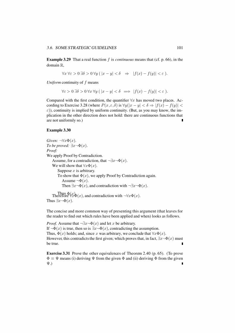
7/16/2019 The Haskell Road to Logic Maths and Programming
http://slidepdf.com/reader/full/the-haskell-road-to-logic-maths-and-programming-5634fa29ef7e9 112/448
3.6. SOME STRATEGIC GUIDELINES 101
Example 3.29 That a real function f is continuous means that (cf. p. 66), in the
domainR,
∀x ∀ε > 0 ∃δ > 0 ∀y ( |x − y| < δ ⇒ |f (x) − f (y)| < ε ).
Uniform continuity of f means
∀ε > 0 ∃δ > 0 ∀x ∀y ( |x − y| < δ =⇒ |f (x) − f (y)| < ε ).
Compared with the first condition, the quantifier ∀x has moved two places. Ac-
cording to Exercise 3.28 (where P (x,ε,δ ) is ∀y(|x − y| < δ ⇒ |f (x) − f (y)| <ε)), continuity is implied by uniform continuity. (But, as you may know, the im-
plication in the other direction does not hold: there are continuous functions that
are not uniformly so.)
Example 3.30
Given: ¬∀xΦ(x).
To be proved: ∃x¬Φ(x).
Proof:
We apply Proof by Contradiction.
Assume, for a contradiction, that ¬∃x¬Φ(x).
We will show that ∀xΦ(x).
Suppose x is arbitrary.
To show that Φ(x), we apply Proof by Contradiction again.
Assume ¬Φ(x).
Then ∃x¬Φ(x), and contradiction with ¬∃x¬Φ(x).
Thus Φ(x).Therefore ∀xΦ(x), and contradiction with ¬∀xΦ(x).
Thus ∃x¬Φ(x).
The concise and more common way of presenting this argument (that leaves for
the reader to find out which rules have been applied and when) looks as follows.
Proof. Assume that ¬∃x¬Φ(x) and let x be arbitrary.
If ¬Φ(x) is true, then so is ∃x¬Φ(x), contradicting the assumption.
Thus, Φ(x) holds; and, since x was arbitrary, we conclude that ∀xΦ(x).
However, this contradicts the first given; which proves that, in fact, ∃x¬Φ(x) must
be true.
Exercise 3.31 Prove the other equivalences of Theorem 2.40 (p. 65). (To prove
Φ ≡ Ψ means (i) deriving Ψ from the given Φ and (ii) deriving Φ from the given
Ψ.)
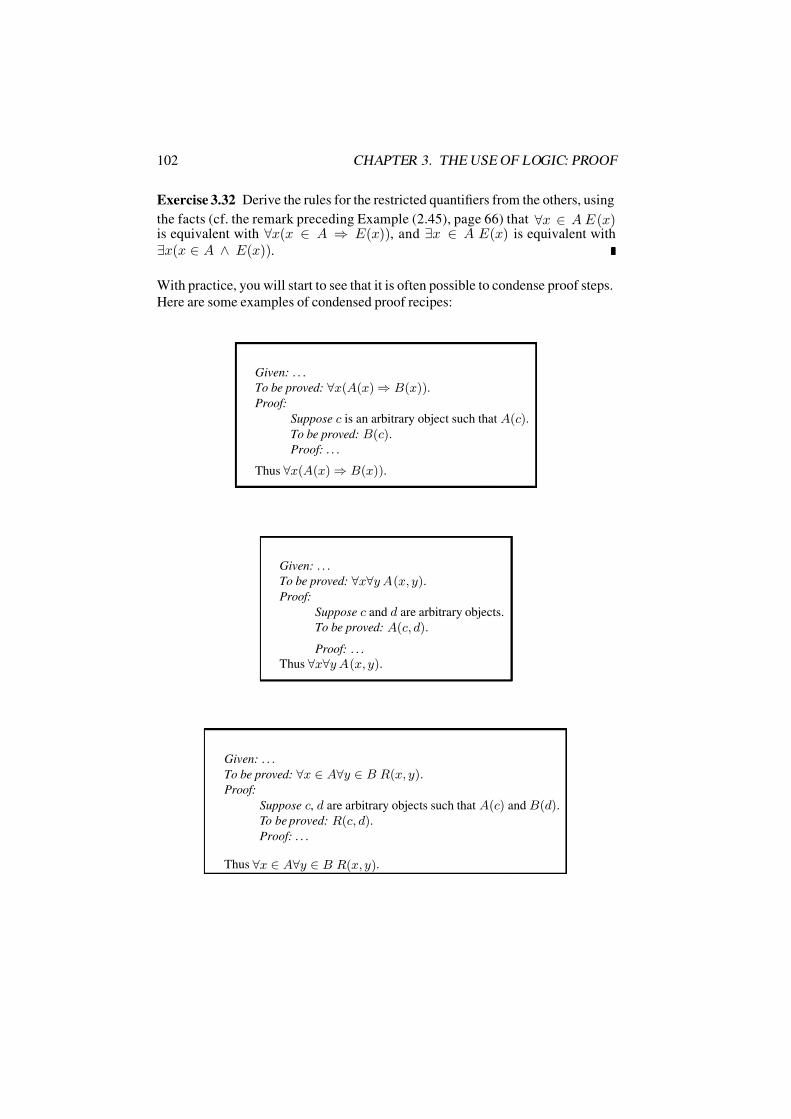
7/16/2019 The Haskell Road to Logic Maths and Programming
http://slidepdf.com/reader/full/the-haskell-road-to-logic-maths-and-programming-5634fa29ef7e9 113/448
102 CHAPTER 3. THE USE OF LOGIC: PROOF
Exercise 3.32 Derive the rules for the restricted quantifiers from the others, using
the facts (cf. the remark preceding Example (2.45), page 66) that ∀x ∈ A E (x)is equivalent with ∀x(x ∈ A ⇒ E (x)), and ∃x ∈ A E (x) is equivalent with
∃x(x ∈ A ∧ E (x)).
With practice, you will start to see that it is often possible to condense proof steps.
Here are some examples of condensed proof recipes:
Given: . . .
To be proved: ∀x(A(x) ⇒ B(x)).
Proof:
Suppose c is an arbitrary object such that A(c).
To be proved: B(c).
Proof: . . .
Thus ∀x(A(x) ⇒ B(x)).
Given: . . .
To be proved: ∀x∀y A(x, y).
Proof:
Suppose c and d are arbitrary objects.
To be proved: A(c, d).
Proof: . . .
Thus ∀x∀y A(x, y).
Given: . . .
To be proved: ∀x ∈ A∀y ∈ B R(x, y).
Proof:
Suppose c, d are arbitrary objects such that A(c) and B(d).
To be proved: R(c, d).
Proof: . . .
Thus ∀x ∈ A∀y ∈ B R(x, y).
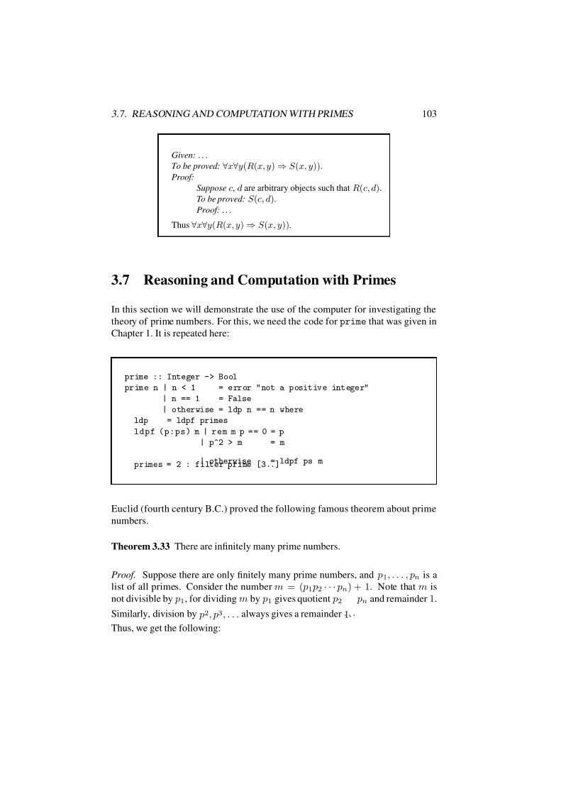
7/16/2019 The Haskell Road to Logic Maths and Programming
http://slidepdf.com/reader/full/the-haskell-road-to-logic-maths-and-programming-5634fa29ef7e9 114/448
3.7. REASONING AND COMPUTATION WITH PRIMES 103
Given: . . .
To be proved: ∀x∀y(R(x, y) ⇒ S (x, y)).
Proof:
Suppose c, d are arbitrary objects such that R(c, d).
To be proved: S (c, d).
Proof: . . .
Thus ∀x∀y(R(x, y) ⇒ S (x, y)).
3.7 Reasoning and Computation with Primes
In this section we will demonstrate the use of the computer for investigating the
theory of prime numbers. For this, we need the code for prime that was given in
Chapter 1. It is repeated here:
prime :: Integer -> Bool
prime n | n < 1 = error "not a positive integer"
| n == 1 = False
| otherwise = ldp n == n where
ldp = ldpf primes
ldpf (p:ps) m | rem m p == 0 = p
| p^2 > m = m
| otherwise = ldpf ps mprimes = 2 : filter prime [3..]
Euclid (fourth century B.C.) proved the following famous theorem about prime
numbers.
Theorem 3.33 There are infinitely many prime numbers.
Proof. Suppose there are only finitely many prime numbers, and p1, . . . , pn is a
list of all primes. Consider the number m = ( p1 p2 · · · pn) + 1. Note that m is
not divisible by p1, for dividing m by p1 gives quotient p2
· · · pn and remainder 1.
Similarly, division by p2, p3, . . . always gives a remainder 1.
Thus, we get the following:

7/16/2019 The Haskell Road to Logic Maths and Programming
http://slidepdf.com/reader/full/the-haskell-road-to-logic-maths-and-programming-5634fa29ef7e9 115/448
104 CHAPTER 3. THE USE OF LOGIC: PROOF
•LD(m) is prime,
• For all i ∈ 1, . . . n, LD(m) = pi.
Thus, we have found a prime number LD(m) different from all the prime numbers
in our list p1, . . . , pn, contradicting the assumption that p1, . . . , pn was the full list
of prime numbers. Therefore, there must be infinitely many prime numbers.
Exercise 3.34 Let A = 4n + 3 | n ∈ N (See Example 5.90 below). Show that
A contains infinitely many prime numbers. (Hint: any prime > 2 is odd, hence of
the form 4n + 1 or 4n + 3. Assume that there are only finitely many primes of
the form 4n + 3, say p1, . . . , pm. Consider the number N = 4 p1 · · · pm − 1 =4( p1 · · · pm − 1) + 3. Argue that N must contain a factor 4q + 3, using the fact
that (4a + 1)(4b + 1) is of the form 4c + 1.)
Use filter prime [ 4*n + 3 | n <- [0..] ] to generatethe primes of this
form.
Euclid’s proof suggests a general recipe for finding bigger and bigger primes.
Finding examples of very large primes is another matter, of course, for how do
you know whether a particular natural number is a likely candidate for a check?
Example 3.35 A famous conjecture made in 1640 by Pierre de Fermat (1601–
1665) is that all numbers of the form
22n + 1
are prime. This holds for n = 0, 1, 2, 3, 4, for we have: 220 + 1 = 21 + 1 = 3,
221
+ 1 = 22
+ 1 = 5, 222
+ 1 = 24
+ 1 = 17, 223
+ 1 = 28
+ 1 = 257, which isprime, and 224 + 1 = 216 + 1 = 65537, which is prime. Apparently, this is as far
as Fermat got.
Our Haskell implementation of prime allows us to refute the conjecture for n = 5,
using the built-in function ^ for exponentiation. We get:
TUOLP> prime (2^2 5 + 1)
False
This counterexample to Fermat’s conjecture was discovered by the mathematician
Leonard Euler (1707–1783) in 1732.
The French priest and mathematician Marin Mersenne (1588–1647; Mersenne was
a pen pal of Descartes) found some large prime numbers by observing that M n =2n − 1 sometimes is prime when n is prime.

7/16/2019 The Haskell Road to Logic Maths and Programming
http://slidepdf.com/reader/full/the-haskell-road-to-logic-maths-and-programming-5634fa29ef7e9 116/448
3.7. REASONING AND COMPUTATION WITH PRIMES 105
Exercise 3.36 It is not very difficult to show that if n is composite, M n = 2n
−1 is
composite too. Show this. (Hint: Assume that n = ab and prove that xy = 2n − 1for the numbers x = 2b − 1 and y = 1 + 2b + 22b + · · · + 2(a−1)b).
But when n is prime, there is a chance that 2n − 1 is prime too. Examples are
22 − 1 = 3, 23 − 1 = 7, 25 − 1 = 31. Such primes are called Mersenne primes.
Example 3.37 Let us use the computer to find one more Mersenne prime. Put the
procedure prime in a file and load it. Next, we use ^ for exponentiation to make a
new Mersenne guess, as follows:
TUOLP> prime 5
True
TUOLP> prime (2^5-1)
TrueTUOLP> 2^5-1
31
TUOLP> prime (2^31-1)
True
TUOLP> 2^31-1
2147483647
TUOLP>
It may interest you to know that the fact that 231 − 1 is a prime was discovered by
Euler in 1750. Using a computer, this fact is a bit easier to check.
We have already seen how to generate prime numbers in Haskell (Examples 1.22and 1.23). We will now present an elegant alternative: a lazy list implementation
of the Sieve of Eratosthenes. The idea of the sieve is this. Start with the list of all
natural numbers 2:
2, 3, 4, 5, 6, 7, 8, 9, 10, 11, 12, 13, 14, 15, 16, 17, 18, 19, 20,
21, 22, 23, 24, 25, 26, 27, 28, 29, 30, 31, 32, 33, 34, 35,
36, 37, 38, 39, 40, 41, 42, 43, 44, 45, 46, 47, 48, . . .
In the first round, mark 2 (the first number in the list) as prime, and mark all mul-
tiples of 2 for removal in the remainder of the list (marking for removal indicated
by over-lining):
2 , 3, 4, 5, 6, 7, 8, 9, 10, 11, 12, 13, 14, 15, 16, 17, 18, 19, 20,
21, 22, 23, 24, 25, 26, 27, 28, 29, 30, 31, 32, 33, 34, 35,
36, 37, 38, 39, 40, 41, 42, 43, 44, 45, 46, 47, 48, . . .

7/16/2019 The Haskell Road to Logic Maths and Programming
http://slidepdf.com/reader/full/the-haskell-road-to-logic-maths-and-programming-5634fa29ef7e9 117/448

7/16/2019 The Haskell Road to Logic Maths and Programming
http://slidepdf.com/reader/full/the-haskell-road-to-logic-maths-and-programming-5634fa29ef7e9 118/448
3.7. REASONING AND COMPUTATION WITH PRIMES 107
[2,3,5,7,11,13,17,19,23,29,31,37,41,43,47,53,59,61,67,71,73,79,
83,89,97,101,103,107,109,113,127,131,137,139,149,151,157,163,167,173,179,181,191,193,197,199,211,223,227,229,233,239,241,251,
257,263,269,271,277,281,283,293,307,311,313,317,331,337,347,349,
353,359,367,373,379,383,389,397,401,409,419,421,431,433,439,443,
449,457,461,463,467,479,487,491,499,503,509,521,523,541,547,557,
563,569,571,577,587,593,599,601,607,613,617,619,631,641,643,647,
653,659,661,673,677,683,691,701,709,719,727,733,739,743,751,757,
761,769,773,787,797,809,811,821,823,827,829,839,853,857,859,863,
877,881,883,887,907,911,919,929,937,941,947,953,967,971,977,983,
991,997,1009,1013,1019,1021,1031,1033,1039,1049,1051,1061,1063,
Interrupted!
Does this stream ever dry up? We know for sure that it doesn’t, because of Euclid’s
proof.
It is possible, by the way, to take a finite initial segment of an infinite Haskell list.
This is done with the built in function take, as follows:
TUOLP> take 100 primes
[2,3,5,7,11,13,17,19,23,29,31,37,41,43,47,53,59,61,67,71,73,79,
83,89,97,101,103,107,109,113,127,131,137,139,149,151,157,163,
167,173,179,181,191,193,197,199,211,223,227,229,233,239,241,251,
257,263,269,271,277,281,283,293,307,311,313,317,331,337,347,349,
353,359,367,373,379,383,389,397,401,409,419,421,431,433,439,443,
449,457,461,463,467,479,487,491,499,503,509,521,523,541]
TUOLP>
Exercise 3.38 A slightly faster way to generate the primes is by starting out from
the odd numbers. The stepping and marking will work as before, for if you countk positions in the odd numbers starting from any odd number a = 2n + 1, you will
move on to number (2n + 1) + 2k, and if a is a multiple of k, then so is a + 2k.
Implement a function fasterprimes :: [Integer] using this idea. The odd
natural numbers, starting from 3, can be generated as follows:
oddsFrom3 :: [Integer]
oddsFrom3 = 3 : map (+2) oddsFrom3
Still faster is to clean up the list at every step, by removing multiples from the list
as you go along. We will come back to this matter in Section 10.1.

7/16/2019 The Haskell Road to Logic Maths and Programming
http://slidepdf.com/reader/full/the-haskell-road-to-logic-maths-and-programming-5634fa29ef7e9 119/448
108 CHAPTER 3. THE USE OF LOGIC: PROOF
Exercise 3.39 Write a Haskell program to refute the following statement about
prime numbers: if p1, . . . , pk are all the primes < n, then ( p1 × · · · × pk) + 1 is aprime.
A computer is a useful instrument for refuting guesses or for checking particular
cases. But if, instead of checking a guess for a particular case, you want to check
the truth of interesting general statements it is of limited help. You can use the
function mersenne to generate Mersenne primes, but the computer will not tell
you whether this stream will dry up or not . . .
mersenne = [ (p,2^p - 1) | p <- primes, prime (2^p - 1) ]
This is what a call to mersenne gives:
TUOLP> mersenne
[(2,3),(3,7),(5,31),(7,127),(13,8191),(17,131071),(19,524287),
(31,2147483647)
If you are interested in how this goes on, you should check out GIMPS (“Great
Internet Mersenne Prime Search”) on the Internet. To generate slightly more in-
formation, we can define:
notmersenne = [ (p,2^p - 1) | p <- primes, not (prime (2^p-1)) ]
This gives:
TUOLP> notmersenne
[(11,2047),(23,8388607),(29,536870911),(37,137438953471),
(41,2199023255551),(43,8796093022207),(47,140737488355327),
(53,9007199254740991),(59,576460752303423487)
The example may serve to illustrate the limits of what you can do with a computer
when it comes to generating mathematical insight. If you make an interesting
mathematical statement, there are three possibilities:

7/16/2019 The Haskell Road to Logic Maths and Programming
http://slidepdf.com/reader/full/the-haskell-road-to-logic-maths-and-programming-5634fa29ef7e9 120/448
3.7. REASONING AND COMPUTATION WITH PRIMES 109
•You succeed in proving it. This establishes the statement as a theorem.
• You succeed in disproving it (with or without the help of a computer). This
establishes the statement as a refuted conjecture.
• Neither of the above. This may indicate that you have encountered an open
problem in mathematics. It may also indicate, of course, that you haven’t
been clever enough.
Example 3.40 Here is an example of an open problem in mathematics:
Are there infinitely many Mersenne primes?
It is easy to see that Euclid’s proof strategy will not work to tackle this problem.The assumption that there is a finite list p1, . . . , pn of Mersenne primes does yield
a larger prime, but nothing guarantees that this larger prime number is again of the
form 2m − 1.
Mersenne primes are related to so-called perfect numbers. A perfect number is a
number n with the curious property that the sum of all its divisors equals 2n, or,
in other words, the sum of all proper divisors of n equals n (we call a divisor d of
n proper if d < n). The smallest perfect number is 6, for its proper divisors are
1, 2 and 3, and 1 + 2 + 3 = 6, and it is easy to check that 1, 2, 3, 4 and 5 are not
perfect.
Euclid proved that if 2n − 1 is prime, then 2n−1(2n − 1) is perfect. Examples of
perfect numbers found by Euclid’s recipe are: 2
·(22
−1) = 6, 22
·(23
−1) = 28,
24 · (25 − 1) = 496.
Exercise 3.41 How would you go about yourself to prove the fact Euclid proved?
Here is a hint: if 2n − 1 is prime, then the proper divisors of 2n−1(2n − 1) are
1, 2, 22, . . . , 2n−1, 2n − 1, 2(2n − 1), 22(2n − 1), . . . , 2n−2(2n − 1).
Here is a function for generating the list of proper divisors of a natural number.
This is not an efficient way to generate proper divisors, but never mind.
pdivisors :: Integer -> [Integer]
pdivisors n = [ d | d <- [1..(n-1)], rem n d == 0 ]

7/16/2019 The Haskell Road to Logic Maths and Programming
http://slidepdf.com/reader/full/the-haskell-road-to-logic-maths-and-programming-5634fa29ef7e9 121/448
110 CHAPTER 3. THE USE OF LOGIC: PROOF
With this it is easy to check that 8128 is indeed a perfect number:
TUOLP> pdivisors 8128
[1,2,4,8,16,32,64,127,254,508,1016,2032,4064]
TUOLP> sum (pdivisors 8128)
8128
Even more spectacularly, we have:
TUOLP> prime (2^13 -1)
True
TUOLP> 2^12 * (2^13 -1)
33550336
TUOLP> pdivisors 33550336
[1,2,4,8,16,32,64,128,256,512,1024,2048,4096,8191,16382,32764,65528,131056,262112,524224,1048448,2096896,4193792,8387584,
16775168]
TUOLP> sum [1,2,4,8,16,32,64,128,256,512,1024,2048,4096,8191,16382,
32764,65528,131056,262112,524224,1048448,2096896,4193792,8387584,
16775168]
33550336
TUOLP>
Prime pairs are pairs ( p, p + 2) where both p and p + 2 are prime. Prime pairs can
be generated as follows:
primePairs :: [(Integer,Integer)]primePairs = pairs primes
where
pairs (x:y:xys) | x + 2 == y = (x,y): pairs (y:xys)
| otherwise = pairs (y:xys)
This gives:
TUOLP> take 50 primePairs
take 50 primePairs
[(3,5),(5,7),(11,13),(17,19),(29,31),(41,43),(59,61),(71,73),
(101,103),(107,109),(137,139),(149,151),(179,181),(191,193),
(197,199),(227,229),(239,241),(269,271),(281,283),(311,313),(347,349),(419,421),(431,433),(461,463),(521,523),(569,571),
(599,601),(617,619),(641,643),(659,661),(809,811),(821,823),

7/16/2019 The Haskell Road to Logic Maths and Programming
http://slidepdf.com/reader/full/the-haskell-road-to-logic-maths-and-programming-5634fa29ef7e9 122/448
3.8. FURTHER READING 111
(827,829),(857,859),(881,883),(1019,1021),(1031,1033),
(1049,1051),(1061,1063),(1091,1093),(1151,1153),(1229,1231),(1277,1279),(1289,1291),(1301,1303),(1319,1321),(1427,1429),
(1451,1453),(1481,1483),(1487,1489)]
TUOLP>
Does this stream ever dry up? We don’t know, for the question whether there are
infinitely many prime pairs is another open problem of mathematics.
Exercise 3.42 A prime triple is a triple ( p, p + 2, p + 4) with p, p + 2, p + 4 all
prime. The first prime triple is (3, 5, 7). Are there any more? Note that instructing
the computer to generate them is no help:
primeTriples :: [(Integer,Integer,Integer)]
primeTriples = triples primes
where
triples (x:y:z:xyzs)
| x + 2 == y && y + 2 == z = (x,y,z) : triples (y:z:xyzs)
| otherwise = triples (y:z:xyzs)
We get:
TUOLP> primeTriples
[(3,5,7)
Still, we can find out the answer . . . How?
Exercise 3.43 Consider the following call:
TUOLP> filter prime [ p^2 + 2 | p <- primes ]
[11
Can you prove that 11 is the only prime of the form p2 + 2, with p prime?
3.8 Further Reading
The distinction between finding meaningful relationships in mathematics on one
hand and proving or disproving mathematical statements on the other is drawn

7/16/2019 The Haskell Road to Logic Maths and Programming
http://slidepdf.com/reader/full/the-haskell-road-to-logic-maths-and-programming-5634fa29ef7e9 123/448
112 CHAPTER 3. THE USE OF LOGIC: PROOF
very clearly in Polya [Pol57]. A good introduction to mathematical reasoning is
[Ecc97]. More detail on the structure of proofs is given by Velleman [Vel94].Automated proof checking in Haskell is treated in [HO00]. An all-time classic in
the presentation of mathematical proofs is [Euc56].

7/16/2019 The Haskell Road to Logic Maths and Programming
http://slidepdf.com/reader/full/the-haskell-road-to-logic-maths-and-programming-5634fa29ef7e9 124/448
Chapter 4
Sets, Types and Lists
Preview
The chapter introduces sets, not by means of a definition but by explaining why
‘set’ is a primitive notion, discusses the process of set formation, and explains
some important operations on sets.
Talking about sets can easily lead to paradox, but such paradoxes can be avoided
either by always forming sets on the basis of a previously given set, or by imposing
certain typing constraints on the expressions one is allowed to use. Section 4.2
explains how this relates to functional programming.
The end of the Chapter discusses various ways of implementing sets using list
representations. The chapter presents ample opportunity to exercise your skills in
writing implementations for set operations and for proving things about sets.
module STAL
where
import List
import DB
113

7/16/2019 The Haskell Road to Logic Maths and Programming
http://slidepdf.com/reader/full/the-haskell-road-to-logic-maths-and-programming-5634fa29ef7e9 125/448
114 CHAPTER 4. SETS, TYPES AND LISTS
4.1 Let’s Talk About Sets
Remarkably, it is not possible to give a satisfactory definition of the notion of a
set. There are several axiomatic approaches to set theory; the standard one (that is
implicitly assumed throughout mathematics) is due to Zermelo and Fraenkel and
dates from the beginning of the 20th century.
Axioms vs. Theorems, Primitive vs. Defined Notions. The truth of a mathemati-
cal statement is usually demonstrated by a proof. Most proofs use results that have
been proved earlier. It follows that some truths must be given outright without
proof. These are called axioms. The choice of axioms often is rather arbitrary.
Criteria can be simplicity or intuitive evidence, but what must be considered an
axiom can also be dictated by circumstance (for instance, a proof cannot be given
within the given context, but in another context a proof would be possible). Inthe present context, we shall accept some of the Zermelo-Fraenkel axioms, as well
as some fundamental properties of the number systems, such as the principle of
mathematical induction for N (see Sections 7.1 and 11.1).
Statements that have been proved are called theorems if they are considered to be
of intrinsic value, and lemmas if they are often used in proving theorems.
Notions are split up in two analogous categories. Their meaning may have been
explained by definitions in terms of other notions. However, the process of defining
notions must have a beginning somewhere. Thus, the need for notions that are
primitive, i.e., undefined.
For instance, we shall consider as undefined here the notions of set and natural
number. Given the notion of a set, that of a function can be defined. However, in a
context that is not set-theoretic, it could well be an undefined notion.
Georg Cantor (1845-1915), the founding father of set theory, gave the following
description.
The Comprehension Principle. A set is a collection into a whole of definite, dis-
tinct objects of our intuition or of our thought. The objects are called the elements
(members) of the set.
Usually, the objects that are used as elements of a set are not sets themselves. To
handle sets of this kind is unproblematic. But it is not excluded at all that members
are sets. Thus, in practice, you can encounter sets of sets of . . . sets.
Notation. If the object a is member of the set A, this is denoted by a ∈ A, or
sometimes by A a. If a is not a member of A, we express this as a /∈ A, or

7/16/2019 The Haskell Road to Logic Maths and Programming
http://slidepdf.com/reader/full/the-haskell-road-to-logic-maths-and-programming-5634fa29ef7e9 126/448
4.1. LET’S TALK ABOUT SETS 115
A
a.
Example: 0 ∈ N, 12 ∈ N, 1
2 ∈ Q.
A set is completely determined by its elements: this is the content of the following
Principle of Extensionality. Sets that have the same elements are equal.
Symbolically, for all sets A and B, it holds that:
∀x(x ∈ A ⇔ x ∈ B) =⇒ A = B.
The converse of this (that equal sets have the same elements) is trivial. The Prin-
ciple of Extensionality is one of Zermelo’s axioms.
Figure 4.1: A set with a proper subset.
Subsets. The set A is called a subset ofthe set B, and B a superset of A; notations:
A ⊆ B, and B ⊇ A, if every member of A is also a member of B. In symbols:
∀x (x ∈ A =⇒ x ∈ B).
If A ⊆ B and A = B, then A is called a proper subset of B.
For instance, 0, 2 is a proper subset of N, and the set of all multiples of 4 is a
proper subset of the set of all even integers.
Note that A = B iff A ⊆ B and B ⊆ A. To show that A = B we therefore either
have to find an object c with c∈
A, c /∈
B (in this case c is a witness of A⊆
B),
or an object c with c /∈ A, c ∈ B (in this case c is a witness of B ⊆ A). A proof of
A = B will in general have the following form:

7/16/2019 The Haskell Road to Logic Maths and Programming
http://slidepdf.com/reader/full/the-haskell-road-to-logic-maths-and-programming-5634fa29ef7e9 127/448
116 CHAPTER 4. SETS, TYPES AND LISTS
Given: . . .
To be proved: A = B.
Proof:
⊆: Let x be an arbitrary object in A.
To be proved: x ∈ B.
Proof:
. . .
Thus x ∈ B.
⊆: Let x be an arbitrary object in B.
To be proved: x ∈ A.
Proof:
. . .
Thus x
∈A.
Thus A = B.
Warning. Sometimes, A ⊆ B is written as A ⊂ B. Other authors use A ⊂ Bto indicate that A is a proper subset of B. In this book we will stick to ⊆, and
to express that A is properly included in B we will always use the conjunction of
A ⊆ B and A = B.
∈ versus ⊆. Beginners often confuse ∈ and ⊆, but these relations are very
different. For instance, A ⊆ B implies that A and B are both sets, whereas
a ∈ B only implies that B is a set. Assuming that numbers are not sets, we have
that 1∈
0, 1, 2
and 1⊆
0, 1, 2
(provided the latter makes sense); whereas
1 ⊆ 0, 1, 2, and 1 ∈ 0, 1, 2.
Theorem 4.1 For all sets A ,B,C , we have that:
1. A ⊆ A (reflexivity),
2. A ⊆ B ∧ B ⊆ A =⇒ A = B (antisymmetry),
3. A ⊆ B ∧ B ⊆ C =⇒ A ⊆ C (transitivity).
Proof. 1.
To be proved: A ⊆ A, i.e., ∀x(x ∈ A ⇒ x ∈ A).
Proof:
Suppose c is any object in A. Then c ∈ A.
Therefore ∀x(x ∈ A ⇒ x ∈ A), i.e., A ⊆ A.

7/16/2019 The Haskell Road to Logic Maths and Programming
http://slidepdf.com/reader/full/the-haskell-road-to-logic-maths-and-programming-5634fa29ef7e9 128/448
4.1. LET’S TALK ABOUT SETS 117
2. This is Extensionality — be it in a somewhat different guise.
3.
To be proved: A ⊆ B ∧ B ⊆ C ⇒ A ⊆ C .Proof:
Suppose A ⊆ B and B ⊆ C .To be proved: A ⊆ C .Proof:
Suppose c is any object in A.
Then by A ⊆ B. c ∈ B, and by B ⊆ C , c ∈ C .Thus ∀x(x ∈ A ⇒ x ∈ C ), i.e., A ⊆ C .
Thus A ⊆ B ∧ B ⊆ C ⇒ A ⊆ C .
Remark. Note that the converse of antisymmetry also holds for⊆. In other words,
if A, B are sets, then A = B iff A ⊆ B and B ⊆ A. It is because of antisymmetry
of the ⊆ relation that a proof that two sets A, B are equal can consist of the two
subproofs mentioned above: the proof of A ⊆ B and the proof of B ⊆ A.
Exercise 4.2 Show that the superset relation also has the properties of Theorem
4.1, i.e., show that ⊇ is reflexive, antisymmetric and transitive.
Enumeration. A set that has only few elements a1, . . . , an can be denoted as
a
1, . . . , a
n.
Extensionality ensures that this denotes exactly one set, for by extensionality the
set is uniquely determined by the fact that it has a1, . . . , an as its members.
Note that x ∈ a1, . . . , an iff x = a1 ∨ · · · ∨ x = an.
Example 4.3 0, 2, 3 is the set the elements of which are 0, 2 and 3. We clearly
have that 3 ∈ 0, 2, 3, and that 4 ∈ 0, 2, 3.
Note that 0, 2, 3 = 2, 3, 0 = 3, 2, 2, 0. Indeed, these sets have the same
elements. Thus:
Order and repetition in this notation are irrelevant.
Exercise 4.4 Show, that 1, 2, 0, 2, 1 = 0, 1, 2.

7/16/2019 The Haskell Road to Logic Maths and Programming
http://slidepdf.com/reader/full/the-haskell-road-to-logic-maths-and-programming-5634fa29ef7e9 129/448
118 CHAPTER 4. SETS, TYPES AND LISTS
An analogue to the enumeration notation is available in Haskell, where [n..m] can
be used for generating a list of items from n to m. This presupposes that n and mare of the same type, and that enumeration makes sense for that type. (Technically,
the type has to be of the class Ord; see 4.2 below.)
Sets that have many elements, in particular, infinite sets, cannot be given in this
way, unless there is some system in the enumeration of their elements. For in-
stance,N = 0, 1, 2, . . . is the set of natural numbers, and 0, 2, 4, . . . is the set
of even natural numbers.
Abstraction. If P (x) is a certain property of objects x, the abstraction
x | P (x) (4.1)
denotes the set of things x that have property P .Thus, for every particular object a, the expression
a ∈ x | P (x) is equivalent with
P (a).
By Extensionality, our talking about the set of x such that P (x) is justified.
The abstraction notation binds the variable x: the set x | P (x) in no way de-
pends on x; x | P (x) = y | P (y).
Usually, the property P will apply to the elements of a previously given set A. In
that case
x∈A | P (x) denotes the set of those elements of A that have property P . For instance, the set
of even natural numbers can be given by
n∈N | n is even .
This way of defining an infinite set can be mimicked in functional programming
by means of so-called list comprehensions, as follows:
naturals = [0..]
evens1 = [ n | n <- naturals , even n ]

7/16/2019 The Haskell Road to Logic Maths and Programming
http://slidepdf.com/reader/full/the-haskell-road-to-logic-maths-and-programming-5634fa29ef7e9 130/448
4.1. LET’S TALK ABOUT SETS 119
Note the similarity between n <- naturals and n
∈N, which is of course in-
tended by the Haskell design team. The expression even n implements the prop-erty ‘n is even’, so we follow the abstraction notation from set theory almost to the
letter. Here is the implementation of the process that generates the odd numbers:
odds1 = [ n | n <- naturals , odd n ]
Back to the notation of set theory. A variation on the above notation for abstraction
looks as follows. If f is an operation, then
f (x)
|P (x)
denotes the set of things of the form f (x) where the object x has the property P .For instance,
2n | n ∈ N is yet another notation for the set of even natural numbers.
And again, we have a counterpart in functional programming. Here it is:
evens2 = [ 2*n | n <- naturals ]
Still, the similarity in notation between the formal definitions and their imple-
mentations should not blind us to some annoying divergences between theory and
practice. The two notations
n2 | n ∈ 0, . . . , 999and
n2 | n ∈ N ∧ n < 1000are equivalent. They are merely two ways of specifying the set of the first 1000square numbers. But the Haskell counterparts behave very differently:
small_squares1 = [ n^2 | n <- [0..999] ]

7/16/2019 The Haskell Road to Logic Maths and Programming
http://slidepdf.com/reader/full/the-haskell-road-to-logic-maths-and-programming-5634fa29ef7e9 131/448
120 CHAPTER 4. SETS, TYPES AND LISTS
A call to the function small_squares1 indeed produces a list of the first thousand
square numbers, and then terminates. Note the use of [0..999] to enumerate afinite list. Not so with the following:
small_squares2 = [ n^2 | n <- naturals , n < 1000 ]
The way this is implemented, n <- naturals generates the infinite list of natu-
ral numbers in their natural order, and n < 1000 tests each number as it is gen-
erated for the property of being less than 1000. The numbers that satisfy the
test are squared and put in the result list. Unlike the previous implementation
small_squares1, the function small_squares2 will never terminate.
Example 4.5 (*The Russell Paradox) It is not true that to every property E there
corresponds a set x | E (x) of all objects that have E . The simplest example
was given by Bertrand Russell (1872–1970). Consider the property of not having
yourself as a member.
Most sets that you are likely to consider have this property: the set of all even
natural numbers is itself not an even natural number, the set of all integers is itself
not an integer, and so on. Call such sets ‘ordinary’. The corresponding abstraction
is R = x | x ∈ x .
It turns out that the question whether the set R itself is ordinary or not is impossible
to answer. For suppose R ∈ R, that is, suppose R is an ordinary set. Ordinary
sets are the sets that do not have themselves as a member, so R does not have
itself as a member, i.e., R /∈ R. Suppose, on the contrary, that R /∈ R, that is, Ris an extraordinary set. Extraordinary sets are the sets that have themselves as a
member, so R has itself as a member, i.e., R ∈ R.
If R were a legitimate set, this would unavoidably lead us to the conclusion that
R ∈ R ⇐⇒ R ∈ R ,
which is impossible.
You do not have to be afraid for paradoxes such as the Russell paradox of Example
4.5. Only properties that you are unlikely to consider give rise to problems. In
particular, if you restrict yourself to forming sets on the basis of a previously given
set A, by means of the recipe
x∈A | E (x) ,

7/16/2019 The Haskell Road to Logic Maths and Programming
http://slidepdf.com/reader/full/the-haskell-road-to-logic-maths-and-programming-5634fa29ef7e9 132/448
4.2. PARADOXES, TYPES AND TYPE CLASSES 121
no problems will ever arise.
Example 4.6 There is no set corresponding to the property F (x) :≡ there is no
infinite sequence x = x0 x1 x2 . . .. To see this, assume to the contrary
that F is such a set. Assume F ∈ F . This implies F F F F . . ., so by the
defining property of F , F /∈ F . Assume F /∈ F . Then by the defining property of
F , there is an infinite sequence F = x0 x1 x2 . . .. Now take the infinite
sequence x1 x2 . . .. By the defining property of F , x1 /∈ F , contradicting
F = x0 x1.
Exercise 4.7* Assume that A is a set of sets. Show that x ∈ A | x ∈ x ∈ A.
It follows from Exercise (4.7) that every set A has a subset B ⊆ A with B /∈ A.
Take B =
x∈
A|
x /∈
x
.
4.2 Paradoxes, Types and Type Classes
It is a well-known fact from the theory of computation that there is no general
test for checking whether a given procedure terminates for a particular input. The
halting problem is undecidable. Intuitively, the reason for this is that the existence
of an algorithm (a procedure which always terminates) for the halting problem
would lead to a paradox very similar to the Russell paradox.
Here is a simple example of a program for which no proof of termination exists:
run :: Integer -> [Integer]
run n | n < 1 = error "argument not positive"
| n = = 1 = [ 1 ]
| even n = n: run (div n 2)
| odd n = n: run (3*n+1)
This gives, e.g.:
STAL> run 5
[5,16,8,4,2,1]
STAL> run 6
[6,3,10,5,16,8,4,2,1]STAL> run 7
[7,22,11,34,17,52,26,13,40,20,10,5,16,8,4,2,1]

7/16/2019 The Haskell Road to Logic Maths and Programming
http://slidepdf.com/reader/full/the-haskell-road-to-logic-maths-and-programming-5634fa29ef7e9 133/448
122 CHAPTER 4. SETS, TYPES AND LISTS
We say that a procedure diverges when it does not terminate or when it aborts with
an error. Stipulating divergence in Haskell is done by means of the predeclaredfunction undefined, which causes an error abortion, just like error. In fact,
Haskell has no way to distinguish between divergence and error abortion.
Now suppose halts can be defined. Then define the procedure funny, in terms of
halts, as follows (the part of a line after -- is a comment; in this case a warning
that funny is no good as Haskell code):
funny x | halts x x = undefined -- Caution: this
| otherwise = True -- will not work
What about the call funny funny? Does this diverge or halt?
Suppose funny funny does not halt. Then by the definition of funny, we are in
the first case. This is the case where the argument of funny, when applied to itself,
halts. But the argument of funny is funny. Therefore, funny funny does halt,
and contradiction.
Suppose funny funny does halt. Then by the definition of funny, we are in the
second case. This is the case where the argument of funny, when applied to itself,
does not halt. But the argument of funny is funny. Therefore, funny funny
does not halt, and contradiction.
Thus, there is something wrong with the definition of funny. The only peculiarity
of the definition is the use of the halts predicate. This shows that such a halts
predicate cannot be implemented.
It should be clear that funny is a rather close analogue to the Russell set x |x /∈ x. Such paradoxical definitions are avoided in functional programming by
keeping track of the types of all objects and operations.
As we have seen, new types can be constructed from old. Derived types are pairs
of integers, lists of characters (or strings), lists of reals, and so on. How does this
type discipline avoid the halting paradox? Consider the definition of funny. It
makes a call to halts. What is the type of halts? The procedure halts takes
as first argument a procedure, say proc, and as second argument an argument to
that procedure, say arg. This means that the two arguments of halts have types
a - > b and a, respectively. and that (proc arg), the result of applying proc to
arg, has type b. But this means that the application halts x x in the definition of
funny is ill-formed, for as we have seen the types of the two arguments to halts
must be different, so the arguments themselves must be different.

7/16/2019 The Haskell Road to Logic Maths and Programming
http://slidepdf.com/reader/full/the-haskell-road-to-logic-maths-and-programming-5634fa29ef7e9 134/448
4.2. PARADOXES, TYPES AND TYPE CLASSES 123
For another example, take the built-in elem operation of Haskell which checks
whether an object is element of a list. This operation is as close as you can getin Haskell to the ‘∈’ relation of set theory. The operation expects that if its first
argument is of certain type a, then its second argument is of type ‘list over a’.
Thus, in Haskell, the question whether R ∈ R does not make sense, for any R: wit-ness the following interaction. In the transcript, Prelude> is the Haskell promptwhen no user-defined files are loaded.
Prelude> elem ’R’ "Russell"
True
Prelude> elem ’R’ "Cantor"
False
Prelude> elem "Russell" "Cantor"
ERROR: Type error in application
*** expression : "Russell" ‘elem‘ "Cantor"
*** term : "Russell"
*** type : String
*** does not match : Char
Prelude>
You would expect from this that elem has type a -> [a] -> Bool, for it takes
an object of any type a as its first argument, then a list over type a, and it returns a
verdict ‘true’ or ‘false’, i.e., an object of type Bool.
Almost, but not quite. The snag is that in order to check if some thing x is an
element of some list of things l, one has to be able to identify things of the type of
x. The objects that can be identified are the objects of the kinds for which equalityand inequality are defined. Texts, potentially infinite streams of characters, are not
of this kind. Also, the Haskell operations themselves are not of this kind, for the
Haskell operations denote computation procedures, and there is no principled way
to check whether two procedures perform the same task.
For suppose there were a test for equality on procedures (implemented functions).
Then the following would be a test for whether a procedure f halts on input x (here
/= denotes inequality):
halts f x = f / = g
where g y | y == x = undefined -- Caution: this
| otherwise = f y -- will not work
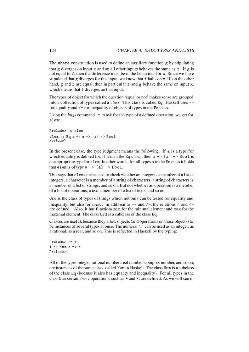
7/16/2019 The Haskell Road to Logic Maths and Programming
http://slidepdf.com/reader/full/the-haskell-road-to-logic-maths-and-programming-5634fa29ef7e9 135/448
124 CHAPTER 4. SETS, TYPES AND LISTS
The where construction is used to define an auxiliary function g by stipulating
that g diverges on input x and on all other inputs behaves the same as f. If g isnot equal to f, then the difference must be in the behaviour for x. Since we have
stipulated that g diverges for this input, we know that f halts on x. If, on the other
hand, g and f are equal, then in particular f and g behave the same on input x,
which means that f diverges on that input.
The types of object for which the question ‘equal or not’ makes sense are grouped
into a collection of types called a class. This class is called Eq . Haskell uses ==
for equality and /= for inequality of objects of types in the Eq class.
Using the hugs command :t to ask for the type of a defined operation, we get forelem:
Prelude> :t elem
elem :: Eq a => a -> [a] -> BoolPrelude>
In the present case, the type judgment means the following. If a is a type for
which equality is defined (or, if a is in the Eq class), then a -> [a] -> Bool is
an appropriate type for elem. In other words: for all types a in the Eq class it holds
that elem is of type a -> [a] -> Bool.
This says that elem can be used to check whether an integer is a member of a list of
integers, a character is a member of a string of characters, a string of characters is
a member of a list of strings, and so on. But not whether an operation is a member
of a list of operations, a text a member of a list of texts, and so on.
Ord is the class of types of things which not only can be tested for equality and
inequality, but also for order : in addition to == and /=, the relations < and <=are defined. Also, it has functions min for the minimal element and max for the
maximal element. The class Ord is a subclass of the class Eq .
Classes are useful, because they allow objects (and operations on those objects) tobe instances of several types at once. The numeral ‘1’ can be used as an integer, asa rational, as a real, and so on. This is reflected in Haskell by the typing:
Prelude> :t 1
1 :: Num a => a
Prelude>
All of the types integer, rational number, real number, complex number, and so on,
are instances of the same class, called Num in Haskell. The class Num is a subclass
of the class Eq (because it also has equality and inequality). For all types in the
class Num certain basic operations, such as + and *, are defined. As we will see in

7/16/2019 The Haskell Road to Logic Maths and Programming
http://slidepdf.com/reader/full/the-haskell-road-to-logic-maths-and-programming-5634fa29ef7e9 136/448
4.3. SPECIAL SETS 125
Chapter 8, addition has different implementations, depending on whether we oper-
ate on N,Z,Q, . . . and depending on the representations we choose. Still, insteadof distinguishing between add, add1, add2, and so on, one could use the same
name for all these different operations. This is standard practice in programming
language design, and it is called operator overloading.
Exercise 4.8 Explain the following error message:
Prelude> elem 1 1
ERROR: [a] is not an instance of class "Num"
Prelude>
4.3 Special Sets
Singletons. Sets that have exactly one element are called singletons. The set
whose only element is a is a ; this is called the singleton of a. Note that it
follows from the definition that x ∈ a iff x = a.
Warning. Do not confuse a singleton a with its element a.
In most cases you will have that a = a. For instance, in the case that a = 0, 1,
we have that 0, 1 = 0, 1. For, 0, 1 has two elements: the numbers 0 and
1. On the other hand, 0, 1 has only one element: the set 0, 1.
Remark. The question whether the equation a = a has solutions (or, more
generally, whether sets a exist such that a ∈ a) is answered differently by different
axiomatizations of set theory. A set satisfying this equation has the shape a =··· ···, but of course this is unofficial notation. For the mathematical
content of set theory this problem is largely irrelevant.
An example of a case where it would be useful to let sets have themselves as
members would be infinite streams, like an infinite list of ‘1’s. Such an object is
easily programmed in Haskell:
ones = 1 : ones
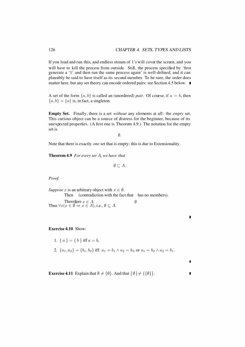
7/16/2019 The Haskell Road to Logic Maths and Programming
http://slidepdf.com/reader/full/the-haskell-road-to-logic-maths-and-programming-5634fa29ef7e9 137/448
126 CHAPTER 4. SETS, TYPES AND LISTS
If you load and run this, and endless stream of 1’s will cover the screen, and you
will have to kill the process from outside. Still, the process specified by ‘firstgenerate a ‘1’ and then run the same process again’ is well-defined, and it can
plausibly be said to have itself as its second member. To be sure, the order does
matter here, but any set theory can encode ordered pairs: see Section 4.5 below.
A set of the form a, b is called an (unordered) pair . Of course, if a = b, then
a, b = a is, in fact, a singleton.
Empty Set. Finally, there is a set without any elements at all: the empty set.
This curious object can be a source of distress for the beginner, because of its
unexpected properties. (A first one is Theorem 4.9.) The notation for the empty
set is
∅.
Note that there is exactly one set that is empty: this is due to Extensionality.
Theorem 4.9 For every set A , we have that
∅ ⊆ A.
Proof.
Suppose x is an arbitrary object with x ∈ ∅.
Then
⊥(contradiction with the fact that
∅has no members).
Therefore x ∈ A.Thus ∀x(x ∈ ∅ ⇒ x ∈ A), i.e., ∅ ⊆ A.
Exercise 4.10 Show:
1. a = b iff a = b,
2. a1, a2 = b1, b2 iff: a1 = b1 ∧ a2 = b2, or a1 = b2 ∧ a2 = b1.
Exercise 4.11 Explain that ∅ = ∅. And that ∅= ∅.

7/16/2019 The Haskell Road to Logic Maths and Programming
http://slidepdf.com/reader/full/the-haskell-road-to-logic-maths-and-programming-5634fa29ef7e9 138/448
4.4. ALGEBRA OF SETS 127
Remark. Abstraction and Restricted Quantification. Note that
∀x ∈ A Φ(x) is true iff x ∈ A | Φ(x) = A.
Similarly,
∃x ∈ A Φ(x) is true iff x ∈ A | Φ(x) = ∅.
4.4 Algebra of Sets
Definition 4.12 (Intersection, Union, Difference.) Assume that A and B are sets.
Then:
1. A ∩ B = x | x ∈ A ∧ x ∈ B is the intersection of A and B,
2. A ∪ B = x | x ∈ A ∨ x ∈ B is their union,
and
3. A − B = x | x ∈ A ∧ x ∈ B their difference.
Types of Set Theoretic Expressions Often, the symbols ∩ and ∪ are confused
with the connectives ∧ and ∨. From Definition 4.12, their intimate connection is
clear. However, their functioning is completely different: ∩ and ∪ produce, given
two sets A and B, new sets A ∩ B resp. A ∪ B (thus, ∩ and ∪ can be written
between sets only), whereas ∧ and ∨ combine two statements Φ and Ψ into newstatements Φ ∧ Ψ resp. Φ ∨ Ψ.
In the idiom of Section 4.2: the operations ∩, ∪ on one hand and ∧, ∨ on the other
have different types. The typing underlying the notation of set theory is much
simpler than that of functional programming. To start with, we just distinguish
between the types s (for set), t (for a proposition, i.e., an expression with a truth
value), (for anything at all), and s (for a family of sets, see below).
t is like Bool in Haskell, but s has no Haskell analogue. In set theory, sets like
N, Z, Q, R are all of the same type, namely s, whereas in Haskell much finer
distinctions are drawn. The simplicity of the typing underlying set theory is an
advantage, for it makes the language of set theory more flexible.
To find the types of the set theoretic operations we use the same recipe as in func-
tional programming. Thus, ∩ and ∪ both have type s → s → s, for they take
two set arguments and produce a new set. ∧ and ∨ have type t → t → t, tor they

7/16/2019 The Haskell Road to Logic Maths and Programming
http://slidepdf.com/reader/full/the-haskell-road-to-logic-maths-and-programming-5634fa29ef7e9 139/448
128 CHAPTER 4. SETS, TYPES AND LISTS
Figure 4.2: Set union, intersection, difference, and complement.

7/16/2019 The Haskell Road to Logic Maths and Programming
http://slidepdf.com/reader/full/the-haskell-road-to-logic-maths-and-programming-5634fa29ef7e9 140/448
4.4. ALGEBRA OF SETS 129
take two propositions and produce a new proposition.
∈has type
→s
→t,
for it takes anything at all as its first argument, a set as its second argument, andproduces a proposition.
Exercise 4.13 What are the types of the set difference operator − and of the in-
clusion operator ⊆ ?
Exercise 4.14 Give the types of the following expressions:
1. x ∈ x | E (x).
2. x | E (x).
3. (A ∩ B) ⊆ C .
4. (A ∪ B) ∩ C .
5. ∀x(x ∈ A ⇒ x ∈ B).
6. A = B.
7. a ∈ A ⇔ a ∈ B.
The relationships between ∩ and ∧ and between ∪ and ∨ become clearer if the
equalities from Definition 4.12 are written in the form of equivalences:
1. x ∈ A ∩ B ⇐⇒ x ∈ A ∧ x ∈ B,
2. x ∈ A ∪ B ⇐⇒ x ∈ A ∨ x ∈ B,
3. x ∈ A − B ⇐⇒ x ∈ A ∧ x ∈ B.
Disjointness. Sets A and B are called disjoint if A ∩ B = ∅.
Example 4.15 For A = 1, 2, 3 and B = 3, 4, we have: A ∪ B = 1, 2, 3, 4,
A ∩ B = 3 and A − B = 1, 2. A and B are not disjoint, for 3 ∈ A ∩ B.
Theorem 4.16 For all sets A , B and C , we have the following:
1. A ∩ ∅ = ∅;
A ∪ ∅ = A ,

7/16/2019 The Haskell Road to Logic Maths and Programming
http://slidepdf.com/reader/full/the-haskell-road-to-logic-maths-and-programming-5634fa29ef7e9 141/448
130 CHAPTER 4. SETS, TYPES AND LISTS
2. A
∩A = A;
A ∪ A = A (idempotence),
3. A ∩ B = B ∩ A;
A ∪ B = B ∪ A (commutativity),
4. A ∩ (B ∩ C ) = (A ∩ B) ∩ C ;
A ∪ (B ∪ C ) = (A ∪ B) ∪ C (associativity),
5. A ∩ (B ∪ C ) = (A ∩ B) ∪ (A ∩ C );
A ∪ (B ∩ C ) = (A ∪ B) ∩ (A ∪ C ) (distributivity).
By part 4.16.4, we can omit parentheses in intersections and unions of more than
two sets.
Proof. Using the definitions of ∩, ∪ and −, these laws all reduce to Theorem 2.10
(p. 45). Still, it is instructive to give a direct proof. Here is one for the first
distribution law:
⊆:
Let x be any object in A ∩ (B ∪ C ).
Then x ∈ A and either x ∈ B or x ∈ C .Suppose x ∈ B. Then x ∈ A ∩ B, so x ∈ (A ∩ B) ∪ (A ∩ C ).
Suppose x ∈ C . Then x ∈ A ∩ C , so x ∈ (A ∩ B) ∪ (A ∩ C ).
Thus in either case x ∈ (A ∩ B) ∪ (A ∩ C ).
Thus A ∩ (B ∪ C ) ⊆ (A ∩ B) ∪ (A ∩ C ).
⊆:Let x be any object in (A ∩ B) ∪ (A ∩ C ).
Then either x ∈ A ∩ B or x ∈ (A ∩ C ).
Suppose x ∈ A ∩ B, i.e., x ∈ A and x ∈ B.
Then x ∈ A and either x ∈ B or x ∈ C , i.e., x ∈ A ∩ (B ∪ C ).
Suppose x ∈ A ∩ C , i.e., x ∈ A and x ∈ C .Then x ∈ A and either x ∈ B or x ∈ C , i.e., x ∈ A ∩ (B ∪ C ).
Thus in either case x ∈ A ∩ (B ∪ C ).
Therefore (A ∩ B) ∪ (A ∩ C ) ⊆ A ∩ (B ∪ C ).
By Extensionality, the required equality follows.
Finally, a third form of proof: using the definitions, the distribution law reduces,
as in the above, to the equivalence
x ∈ A ∧ (x ∈ B ∨ x ∈ C ) ⇐⇒ (x ∈ A ∧ x ∈ B) ∨ (x ∈ A ∧ x ∈ C ),

7/16/2019 The Haskell Road to Logic Maths and Programming
http://slidepdf.com/reader/full/the-haskell-road-to-logic-maths-and-programming-5634fa29ef7e9 142/448
4.4. ALGEBRA OF SETS 131
which involves the three statements x
∈A, x
∈B and x
∈C . That this comes
out true always can be checked using an 8-line truth table in the usual way.
Exercise 4.17 A, B and C are sets. Show:
1. A ⊆ B ⇔ A − B = ∅.
2. A ∩ B = A − (A − B).
Example 4.18 We show that A − C ⊆ (A − B) ∪ (B − C ).
Given: x∈
(A−
C ).To be proved: x ∈ (A − B) ∨ x ∈ (B − C ).
Proof:
Suppose x ∈ B. From x ∈ (A − C ) we get that x /∈ C , so x ∈ (B − C ).
Therefore x ∈ (A − B) ∨ x ∈ (B − C ).
Suppose x /∈ B. From x ∈ (A − C ) we get that x ∈ A, so x ∈ (A − B).
Therefore x ∈ (A − B) ∨ x ∈ (B − C ).
Thus x ∈ (A − B) ∨ x ∈ (B − C ).
Exercise 4.19 Express (A ∪ B) ∩ (C ∪ D) as a union of four intersections.
Complement. Fix a set X , of which all sets to be considered are subsets. The
complement Ac of a set A ⊆ X is now defined by
Ac := X − A.
Clearly, we have that for all x ∈ X :
x ∈ Ac ⇔ x ∈ A.
Theorem 4.20
1. (Ac)c = A;
X c = ∅;
∅c = X ,

7/16/2019 The Haskell Road to Logic Maths and Programming
http://slidepdf.com/reader/full/the-haskell-road-to-logic-maths-and-programming-5634fa29ef7e9 143/448
132 CHAPTER 4. SETS, TYPES AND LISTS
2. A
∪Ac = X ;
A ∩ Ac = ∅ ,
3. A ⊆ B ⇔ Bc ⊆ Ac ,
4. (A ∪ B)c = Ac ∩ Bc;
(A ∩ B)c = Ac ∪ Bc (DeMorgan laws).
Figure 4.3: Symmetric set difference.
Symmetric Difference. The symmetric difference of two sets A and B, notation
A ⊕ B, is the set given by x | x ∈ A ⊕ x ∈ B. This is the set of all objects that
are either in A or in B, but not in both.
Exercise 4.21 Show that A
⊕B = (A
−B)
∪(B
−A) = (A
∪B)
−(A
∩B).
1, 2, 31, 2 2, 3 1, 31 2 3
∅
Figure 4.4: The power set of 1, 2, 3.
Definition 4.22 (Power Set) The powerset of the set X is the set ℘(X ) = A|A ⊆X of all subsets of X .
By Theorem 4.9 and 4.1.1 we have that ∅ ∈ ℘(X ) and X ∈ ℘(X ). So, for
instance, ℘(∅, 1) = ∅, ∅, 1, ∅, 1. Note that X ∈ ℘(A) ⇔ X ⊆ A.

7/16/2019 The Haskell Road to Logic Maths and Programming
http://slidepdf.com/reader/full/the-haskell-road-to-logic-maths-and-programming-5634fa29ef7e9 144/448
4.4. ALGEBRA OF SETS 133
Exercise 4.23 Let X be a set with at least two elements. Then by Theorem (4.1),
the relation ⊆ on ℘(X ) has the properties of reflexivity, antisymmetry and transi-tivity. The relation on R also has these properties. The relation on R has the
further property of linearity: for all x, y ∈ R, either x y or y x. Show that ⊆on ℘(X ) lacks this property.
Figure 4.5: Generalized set union and intersection.
Definition 4.24 (Generalized Union and Intersection) Suppose that a set Ai has
been given for every element i of a set I .
1. The union of the sets Ai is the set x | ∃i∈I (x ∈ Ai).
Notation:
i∈I Ai.
2. The intersection of the sets Ai is the set x | ∀i∈I (x ∈ Ai).Notation:
i∈I Ai
If the elements of I are sets themselves, and Ai = i (i ∈ I ), theni∈I i is called
the union of I ;
The short notation for this set is
I . Similarly,i∈I i is written as
I .
In the case that I = N,i∈I Ai and
i∈I Ai can also be written as A0 ∪ A1 ∪
A2 ∪ · · · , resp., A0 ∩ A1 ∩ A2 ∩ · · · .
A set of sets is sometimes called a family of sets or a collection of sets. If F is a
family of sets,
F and
F are sets. For example, if
F = 1, 2, 3, 2, 3, 4, 3, 4, 5,
thenF = 1, 2, 3, 4, 5 and
F = 3.

7/16/2019 The Haskell Road to Logic Maths and Programming
http://slidepdf.com/reader/full/the-haskell-road-to-logic-maths-and-programming-5634fa29ef7e9 145/448
134 CHAPTER 4. SETS, TYPES AND LISTS
Example 4.25 For p
∈N, let A p =
mp
|m
∈N, m 1
. Then A p is the set of
all natural numbers that have p as a factor.i∈2,3,5,7 Ai is the set of all natural numbers of the form n · 2α3β5γ 7δ, with at
least one of α, β,γ,δ > 0.i∈2,3,5,7 Ai is the set of all natural numbers of the form n · 2α3β5γ 7δ, with all
of α, β,γ,δ > 0, which is the set A210.
Let F and G be collections of sets. To check the truth of statements such asF ⊆G it is often useful to analyze their logical form by means of a translation in
terms of quantifiers and the relation ∈. The translation of F ⊆ G becomes:
∀x(∃y(y ∈ F ∧ x ∈ y) ⇒ ∀z(z ∈ G ⇒ x ∈ z)).
Exercise 4.26 Give a logical translation of F ⊆ G using only the relation ∈.
Types of Generalized Union and Intersection Again, it is useful to consider the
types of the operations of generalized union and intersection. These operations
take families of sets and produce sets, so their type is s → s, where s is the
type of a family of sets.
Exercise 4.27 Let F be a family of sets. Show that there is a set A with the
following properties:
1. F ⊆ ℘(A),
2. For all sets B: if F ⊆ ℘(B) then A ⊆ B.
Remark. If I = ∅, theni∈I Ai = ∅, and
i∈I Ai is the collection of all sets.
This last fact is an example of a trivially true implication: if I = ∅, then every
statement i ∈ I is false, hence the implication i ∈ I ⇒ x ∈ Ai true, and
everything is member of
x
| ∀i
∈I (x
∈Ai)
=
x
| ∀i(i
∈I
⇒x
∈Ai)
.
Therefore, the notationi∈I Ai usually presupposes that I = ∅.

7/16/2019 The Haskell Road to Logic Maths and Programming
http://slidepdf.com/reader/full/the-haskell-road-to-logic-maths-and-programming-5634fa29ef7e9 146/448
4.4. ALGEBRA OF SETS 135
Example 4.28 For x
∈X , we have that:
x ∈ (A ∪ B)c ⇔ ¬(x ∈ A ∪ B)
⇔ ¬(x ∈ A ∨ x ∈ B)∗⇔ ¬x ∈ A ∧ ¬x ∈ B
⇔ x ∈ Ac ∧ x ∈ Bc
⇔ x ∈ Ac ∩ Bc.
Step (∗) is justified by propositional reasoning. See 2.10.9. Extensionality allows
us to conclude the first DeMorgan law:
(A ∪ B)c = Ac ∩ Bc.
Exercise 4.29 Prove the rest of Theorem 4.20.
Exercise 4.30 Answer as many of the following questions as you can.
1. Determine: ℘(∅), ℘(℘(∅)) and ℘(℘(℘(∅))).
2. How many elements has ℘5(∅) = ℘(℘(℘(℘(℘(∅)))))?
3. How many elements has ℘(A), given that A has n elements?
Exercise 4.31 Check whether the following is true: if two sets have the same
subsets, then they are equal. I.e.: if ℘(A) = ℘(B), then A = B. Give a proof or a
refutation by means of a counterexample.
Exercise 4.32 Is it true that for all sets A and B:
1. ℘(A ∩ B) = ℘(A) ∩ ℘(B)?
2. ℘(A ∪ B) = ℘(A) ∪ ℘(B)?
Provide either a proof or a refutation by counter-example.
Exercise 4.33* Show:
1. B ∩ (i∈I Ai) =
i∈I (B ∩ Ai),

7/16/2019 The Haskell Road to Logic Maths and Programming
http://slidepdf.com/reader/full/the-haskell-road-to-logic-maths-and-programming-5634fa29ef7e9 147/448
136 CHAPTER 4. SETS, TYPES AND LISTS
2. B
∪(i
∈I Ai) = i
∈I (B
∪Ai),
3. (i∈I Ai)
c =i∈I A
ci , assuming that ∀i ∈ I Ai ⊆ X ,
4. (i∈I Ai)
c =i∈I A
ci , assuming that ∀i ∈ I Ai ⊆ X .
Exercise 4.34* Assume that you are given a certain set A0. Suppose you are as-
signed the task of finding sets A1, A2, A3, . . . such that ℘(A1) ⊆ A0, ℘(A2) ⊆A1, ℘(A3) ⊆ A2,. . . Show that no matter how hard you try, you will eventually
fail, that is: hit a set An for which no An+1 exists such that ℘(An+1) ⊆ An. (I.e.,
∅ ∈ An.)
Hint. Suppose you can go on forever. Show this would entail ℘(i
∈N
Ai)
⊆i∈N Ai. Apply Exercise 4.7.
Exercise 4.35* Suppose that the collection K of sets satisfies the following condi-
tion:
∀A ∈ K(A = ∅ ∨ ∃B ∈ K(A = ℘(B))).
Show that every element of K has the form ℘n(∅) for some n ∈ N. (N.B.: ℘0(∅) =∅.)
4.5 Ordered Pairs and Products
Next to the unordered pairs
a, b
of Section 4.3, in which the order of a and b is
immaterial (a, b = b, a), there are ordered pairs in which order does count.
The ordered pair of objects a and b is denoted by
(a, b) .
Here, a is the first and b the second coordinate of (a, b).
Ordered pairs behave according to the following rule:
(a, b) = (x, y) =⇒ a = x ∧ b = y. (4.2)
This means that the ordered pair of a and b fixes the objects as well as their order.
Its behaviour differs from that of the unordered pair: we always have that a, b =
b, a
, whereas (a, b) = (b, a) only holds — according to (4.2) — when a = b.
Warning. If a and b are reals, the notation (a, b) also may denote the open interval
x ∈ R | a < x < b. The context should tell you which of the two is meant.

7/16/2019 The Haskell Road to Logic Maths and Programming
http://slidepdf.com/reader/full/the-haskell-road-to-logic-maths-and-programming-5634fa29ef7e9 148/448
4.5. PAIRS AND PRODUCTS 137
Defining Ordered Pairs. Defining
(a, b) = a, a, ballows you to prove (4.2). Cf. Exercise 4.41.
Definition 4.36 (Products) The (Cartesian) product of the sets A and B is the set
of all pairs (a, b) where a ∈ A and b ∈ B. In symbols:
A × B = (a, b) | a ∈ A ∧ b ∈ B .
Instead of A × A one usually writes A2.
Example 4.37 0, 1 × 1, 2, 3 = (0, 1), (0, 2), (0, 3), (1, 1), (1, 2), (1, 3).
When A and B are real intervals on the X resp., the Y -axis in two-dimensional
space, A × B can be pictured as a rectangle.
Ran(R)
Dom(R)
R
Theorem 4.38 For arbitrary sets A ,B,C,D the following hold:
1. (A × B) ∩ (C × D) = (A × D) ∩ (C × B),
2. (A ∪ B) × C = (A × C ) ∪ (B × C ); (A ∩ B) × C = (A × C ) ∩ (B × C ),
3. (A ∩ B) × (C ∩ D) = (A × C ) ∩ (B × D),
4. (A ∪ B) × (C ∪ D) = (A × C ) ∪ (A × D) ∪ (B × C ) ∪ (B × D),
5. [(A − C ) × B] ∪ [A × (B − D)] ⊆ (A × B) − (C × D).
7/16/2019 The Haskell Road to Logic Maths and Programming
http://slidepdf.com/reader/full/the-haskell-road-to-logic-maths-and-programming-5634fa29ef7e9 149/448
138 CHAPTER 4. SETS, TYPES AND LISTS
Proof. As an example, we prove the first item of part 2.
To be proved: (A ∪ B) × C = (A × C ) ∪ (B × C ):
⊆:
Suppose that p ∈ (A ∪ B) × C . Then a ∈ A ∪ B and c ∈ C exist such that p = (a, c).
Thus (i) a ∈ A or (ii) a ∈ B.
(i). In this case, p ∈ A × C , and hence p ∈ (A × C ) ∪ (B × C ).
(ii). Now p ∈ B × C , and hence again p ∈ (A × C ) ∪ (B × C ).
Thus p ∈ (A × C ) ∪ (B × C ).
Therefore, (A ∪ B) × C ⊆ (A × C ) ∪ (B × C ).
⊆:
Conversely, assume that p ∈ (A × C ) ∪ (B × C ).
Thus (i) p
∈A
×C or (ii) p
∈B
×C .
(i). In this case a ∈ A and c ∈ C exist such that p = (a, c);a fortiori, a ∈ A ∪ B and hence p ∈ (A ∪ B) × C .(ii). Now b ∈ B and c ∈ C exist such that p = (b, c);
a fortiori b ∈ A ∪ B and hence, again, p ∈ (A ∪ B) × C .Thus p ∈ (A ∪ B) × C .
Therefore, (A × C ) ∪ (B × C ) ⊆ (A ∪ B) × C .
The required result follows using Extensionality.
Exercise 4.39 Prove the other items of Theorem 4.38.
Exercise 4.40 1. Assume that A and B are non-empty and that A × B =B × A. Show that A = B.
2. Show by means of an example that the condition of non-emptiness in 1 is
necessary. (Did you use this in your proof of 1?)
Exercise 4.41* To show that defining (a, b) as a, a, b works, prove that
1. a, b = a, c =⇒ b = c,
2.
a
,
a, b
=
x
,
x, y
=
⇒a = x
∧b = y.

7/16/2019 The Haskell Road to Logic Maths and Programming
http://slidepdf.com/reader/full/the-haskell-road-to-logic-maths-and-programming-5634fa29ef7e9 150/448
4.6. LISTS AND LIST OPERATIONS 139
If we assume the property of ordered pairs (a, b) = (x, y) =
⇒a = x
∧b = y, we
can define triples by (a,b,c) := (a, (b, c)). For suppose (a,b,c) = (x,y,z). Thenby definition, (a, (b, c)) = (a,b,c) = (x,y,z) = (x, (y, z)), and by the property
of ordered pairs, we have that a = x and (b, c) = (y, z). Again, by the property
of ordered pairs, b = y and c = z. This shows that (a,b,c) = (x,y,z) ⇒ (a =x ∧ b = y ∧ c = z).
Let us go about this more systematically, by defining ordered n-tuples over some
base set A, for every n ∈ N. We proceed by recursion.
Definition 4.42 (n-tuples over A)
1. A0 := ∅,
2. A
n+1
:= A × A
n
.
In Haskell, ordered pairs are written as (x1,x2), and there are predefined func-tions fst to get at the first member and snd to get at the second member. Orderedtriples are written as (x1, x2, x3), and so on. If x1 has type a and x2 has typeb, then (x1,x2) has type (a,b). Think of this type as the product of the types forx1 and x2. Here is an example:
Prelude> :t (1, ’A’)
(1,’A’) :: Num a => (a,Char)
Prelude>
4.6 Lists and List Operations
Assuming the list elements are all taken from a set A, the set of all lists over Ais the set
n∈N An. We abbreviate this set as A∗. For every list L ∈ A∗ there is
some n ∈ N with L ∈ An. If L ∈ An we say that list L has length n.
Standard notation for the (one and only) list of length 0 is []. A list of length n > 0looks like (x0, (x1, (· · · , xn−1) · · · )). This is often written as [x0, x1, . . . , xn−1].
A one element list is a list of the form (x, []). In line with the above square bracket
notation, this is written as [x].
If one uses lists to represent sets, there is a difficulty. The list [a,b,b] is different
from the list [a, b], for [a,b,b] has length 3, and [a, b] has length 2, but the sets
a,b,b
and
a, b
are identical. This shows that sets and lists have different
identity conditions.
This is how the data type of lists is (pre-)declared in Haskell:

7/16/2019 The Haskell Road to Logic Maths and Programming
http://slidepdf.com/reader/full/the-haskell-road-to-logic-maths-and-programming-5634fa29ef7e9 151/448
140 CHAPTER 4. SETS, TYPES AND LISTS
data [a] = [] | a : [a] deriving (Eq, Ord)
To grasp what this means, recall that in functional programming every set has a
type. The data declaration for the type of lists over type a, notation [a] specifies
that lists over type a are either empty or they consist of an element of type a put in
front of a list over type a. Haskell uses : for the operation of putting an element in
front of a list.
The operation : combines an object with a list of objects of the same type to forma new list of objects of that type. This is reflected by the type judgment:
Prelude> :t (:)
(:) :: a -> [a] -> [a]
The data declaration for lists also tells us, by means of deriving (Eq,Ord), that
if equality is defined on the objects of type a (i.e., if the type a belongs to the class
Eq ) then this relation carries over to lists over type a, and if the objects of type a
are ordered, i.e., if the type a belongs to the class Ord (e.g., the objects of type Z
are ordered by <), then this order carries over to lists over type a.
If we have an equality test for members of the set A, then it is easy to see how
equality can be defined for lists over A (in fact, this is all taken care of by the
predefined operations on lists). Lists are ordered sets, so two lists are the same if
(i) they either are both empty, or (ii) they start with the same element (here is where
the equality notion for elements from A comes in), and their tails are the same. In
Haskell, this is implemented as follows (this is a definition from Prelude.hs):
instance Eq a => Eq [a] where
[] == [] = True
(x:xs) == (y:ys) = x==y && xs==ys
_ == _ = False
This says that if a is an instance of class Eq , then [a] is so too. This specifies how
the equality notion for objects of type a carries over to objects of type [a] (i.e.,
lists over that type). As we have seen, Haskell uses == for equality and = for the
definition of operator values. Part (i) of the definition of list equality is taken care
of by the statement that [] == [] is true, part (ii) is covered by:
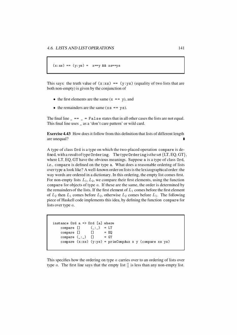
7/16/2019 The Haskell Road to Logic Maths and Programming
http://slidepdf.com/reader/full/the-haskell-road-to-logic-maths-and-programming-5634fa29ef7e9 152/448
4.6. LISTS AND LIST OPERATIONS 141
(x:xs) == (y:ys) = x==y && xs==ys
This says: the truth value of (x:xs) == (y:ys) (equality of two lists that are
both non-empty) is given by the conjunction of
• the first elements are the same (x = = y), and
• the remainders are the same (xs == ys).
The final line _ == _ = False states that in all other cases the lists are not equal.
This final line uses _ as a ‘don’t care pattern’ or wild card.
Exercise 4.43 How does it follow from this definition that lists of different length
are unequal?
A type of class Ord is a type on which the two-placed operation compare is de-
fined, with a result of type Ordering. The type Ordering isthe set LT, EQ, GT,
where LT, EQ, GT have the obvious meanings. Suppose a is a type of class Ord,
i.e., compare is defined on the type a. What does a reasonable ordering of lists
over type a look like? A well-known order on lists is the lexicographical order: the
way words are ordered in a dictionary. In this ordering, the empty list comes first.
For non-empty lists L1, L2, we compare their first elements, using the function
compare for objects of type a. If these are the same, the order is determined by
the remainders of the lists. If the first element of L1 comes before the first element
of L2 then L1 comes before L2, otherwise L2 comes before L1. The following
piece of Haskell code implements this idea, by defining the function compare for
lists over type a.
instance Ord a => Ord [a] where
compare [] (_:_) = LT
compare [] [] = EQ
compare (_:_) [] = GT
compare (x:xs) (y:ys) = primCompAux x y (compare xs ys)
This specifies how the ordering on type a carries over to an ordering of lists over
type a. The first line says that the empty list [] is less than any non-empty list.

7/16/2019 The Haskell Road to Logic Maths and Programming
http://slidepdf.com/reader/full/the-haskell-road-to-logic-maths-and-programming-5634fa29ef7e9 153/448
142 CHAPTER 4. SETS, TYPES AND LISTS
The second line says that the empty list is equal to itself. The third line says that
any non-empty list is greater than the empty list. This fully determines the relationbetween [] and any list. The last line uses an auxiliary function primCompAux to
cover the case of two non-empty lists. This function is defined by:
primCompAux :: Ord a => a -> a -> Ordering -> Ordering
primCompAux x y o =
case compare x y of EQ -> o;
LT -> LT;
GT -> GT
The type declaration of primCompAux says that if a is an ordered type, thenprimCompAux expects three arguments, the first one of type a, the second one
of type a and the third one an element of the set (or type) Ordering, i.e., the set
LT, EQ, GT. The result is again a member of the type Ordering.
The definition of the operation primCompAux uses a case construction, using the
reserved keywords case and of, and the arrow -> to point at the results for the
various cases. . It says that in case the first two arguments are equal, the function
returns the element of Ordering which is its third argument, in case the first ar-
gument is less than the second argument, the function returns LT, in case the first
argument is greater than the second argument, the function returns GT.
Exercise 4.44 Another ordering of lists is as follows: shorter lists come before
longer ones, and for lists of the same length we compare their first elements, and
if these are the same, the remainder lists. Give a formal definition of this ordering.How would you implement it in Haskell?
In list processing, fundamental operations are checking whether a list is empty,
accessing the first element of a non-empty list, determining what remains after
removal of the first element from a list (its tail). The operations for accessing the
head or the tail of a list are implemented in Haskell as follows:
head :: [a] -> a
head (x:_) = x
tail :: [a] -> [a]
tail (_:xs) = xs

7/16/2019 The Haskell Road to Logic Maths and Programming
http://slidepdf.com/reader/full/the-haskell-road-to-logic-maths-and-programming-5634fa29ef7e9 154/448
4.6. LISTS AND LIST OPERATIONS 143
The type of the operation head: give it a list over type a and the operation will
return an element of the same type a. This is specified in head :: [a] -> a.The type of the operation tail is: give it a list over type a and it will return a list
over the same type. This is specified in tail :: [a] -> [a].
Note that these operations are only defined on non-empty lists. (x:_) specifies
the pattern of a non-empty list with first element x, where the nature of the tail is
irrelevant. (_:xs) specifies the pattern of a non-empty list with tail xs, where the
nature of the first element is irrelevant.
Accessing the last element of a non-empty list is done by means of recursion: the
last element of a unit list [x] is equal to [x]. The last element of a non-unit list is
equal to the last element of its tail. Here is the Haskell implementation:
last :: [a] -> a
last [x] = x
last (_:xs) = last xs
Note that because the list patterns [x] and (_:xs) are tried for in that order, the
pattern (_:xs) in this definition matches non-empty lists that are not unit lists.
Exercise 4.45 Which operation on lists is specified by the Haskell definition in
the frame below?
init :: [a] -> [a]init [x] = []
init (x:xs) = x : init xs
It is often useful to be able to test whether a list is empty or not. The following
operation accomplishes this:
null :: [a] -> Bool
null [] = True
null (_:_) = False
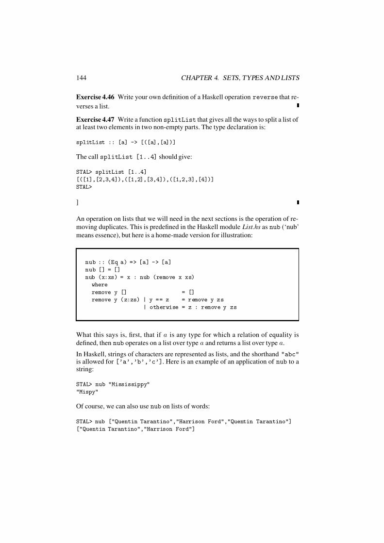
7/16/2019 The Haskell Road to Logic Maths and Programming
http://slidepdf.com/reader/full/the-haskell-road-to-logic-maths-and-programming-5634fa29ef7e9 155/448
144 CHAPTER 4. SETS, TYPES AND LISTS
Exercise 4.46 Write your own definition of a Haskell operation reverse that re-
verses a list.
Exercise 4.47 Write a function splitList that gives all the ways to split a list of at least two elements in two non-empty parts. The type declaration is:
splitList :: [a] -> [([a],[a])]
The call splitList [1..4] should give:
STAL> splitList [1..4]
[([1],[2,3,4]),([1,2],[3,4]),([1,2,3],[4])]
STAL>
]
An operation on lists that we will need in the next sections is the operation of re-
moving duplicates. This is predefined in the Haskell module List.hs as nub (‘nub’
means essence), but here is a home-made version for illustration:
nub :: (Eq a) => [a] -> [a]
nub [] = []
nub (x:xs) = x : nub (remove x xs)
where
remove y [] = []
remove y (z:zs) | y == z = remove y zs
| otherwise = z : remove y zs
What this says is, first, that if a is any type for which a relation of equality is
defined, then nub operates on a list over type a and returns a list over type a.
In Haskell, strings of characters are represented as lists, and the shorthand "abc"is allowed for [’a’,’b’,’c’]. Here is an example of an application of nub to astring:
STAL> nub "Mississippy"
"Mispy"
Of course, we can also use nub on lists of words:
STAL> nub ["Quentin Tarantino","Harrison Ford","Quentin Tarantino"]
["Quentin Tarantino","Harrison Ford"]

7/16/2019 The Haskell Road to Logic Maths and Programming
http://slidepdf.com/reader/full/the-haskell-road-to-logic-maths-and-programming-5634fa29ef7e9 156/448
4.7. LIST COMPREHENSION AND DATABASE QUERY 145
4.7 List Comprehension and Database Query
To get more familiar with list comprehensions, we will devote this section to list
comprehension for database query, using the movie database module DB.hs given
in Figure 4.6. The database that gets listed here is called db, with type DB, where
DB is a synonym for the type [WordList], where Wordlist is again a synonym
for the type [String]. The reserved keyword type is used to declare these type
synonyms. Notice the difference between defining a type synonym with type and
declaring a new data type with data.
The database can be used to define the following lists of database objects, with list
comprehension. Here db :: DB is the database list.
characters = nub [ x | ["play",_,_,x] <- db ]
movies = [ x | ["release",x,_] <- db ]
actors = nub [ x | ["play",x,_,_] <- db ]
directors = nub [ x | ["direct",x,_] <- db ]
dates = nub [ x | ["release",_,x] <- db ]
universe = nub (characters++actors++directors++movies++dates)
Next, define lists of tuples, again by list comprehension:
direct = [ (x,y) | ["direct",x,y] <- db ]
act = [ (x,y) | ["play",x,y,_] <- db ]
play = [ (x,y,z) | ["play",x,y,z] <- db ]
release = [ (x,y) | ["release",x,y] <- db ]
Finally, define one placed, two placed and three placed predicates by means of
lambda abstraction.
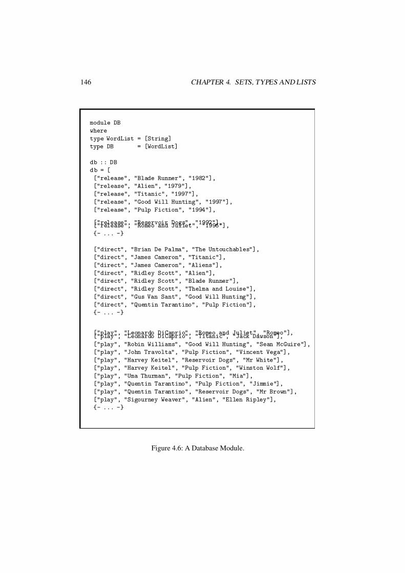
7/16/2019 The Haskell Road to Logic Maths and Programming
http://slidepdf.com/reader/full/the-haskell-road-to-logic-maths-and-programming-5634fa29ef7e9 157/448
146 CHAPTER 4. SETS, TYPES AND LISTS
module DB
where
type WordList = [String]
type DB = [WordList]
db :: DB
d b = [
["release", "Blade Runner", "1982"],
["release", "Alien", "1979"],
["release", "Titanic", "1997"],
["release", "Good Will Hunting", "1997"],
["release", "Pulp Fiction", "1994"],
["release", "Reservoir Dogs", "1992"],["release", "Romeo and Juliet", "1996"],
- ... -
["direct", "Brian De Palma", "The Untouchables"],
["direct", "James Cameron", "Titanic"],
["direct", "James Cameron", "Aliens"],
["direct", "Ridley Scott", "Alien"],
["direct", "Ridley Scott", "Blade Runner"],
["direct", "Ridley Scott", "Thelma and Louise"],
["direct", "Gus Van Sant", "Good Will Hunting"],
["direct", "Quentin Tarantino", "Pulp Fiction"],
- ... -
["play", "Leonardo DiCaprio", "Romeo and Juliet", "Romeo"],["play", "Leonardo DiCaprio", "Titanic", "Jack Dawson"],
["play", "Robin Williams", "Good Will Hunting", "Sean McGuire"],
["play", "John Travolta", "Pulp Fiction", "Vincent Vega"],
["play", "Harvey Keitel", "Reservoir Dogs", "Mr White"],
["play", "Harvey Keitel", "Pulp Fiction", "Winston Wolf"],
["play", "Uma Thurman", "Pulp Fiction", "Mia"],
["play", "Quentin Tarantino", "Pulp Fiction", "Jimmie"],
["play", "Quentin Tarantino", "Reservoir Dogs", "Mr Brown"],
["play", "Sigourney Weaver", "Alien", "Ellen Ripley"],
- ... -
Figure 4.6: A Database Module.

7/16/2019 The Haskell Road to Logic Maths and Programming
http://slidepdf.com/reader/full/the-haskell-road-to-logic-maths-and-programming-5634fa29ef7e9 158/448
4.7. LIST COMPREHENSION AND DATABASE QUERY 147
charP = \ x -> elem x charactersactorP = \ x -> elem x actors
movieP = \ x -> elem x movies
directorP = \ x -> elem x directors
dateP = \ x -> elem x dates
actP = \ (x,y) -> elem (x,y) act
releaseP = \ (x,y) -> elem (x,y) release
directP = \ (x,y) -> elem (x,y) direct
playP = \ (x,y,z) -> elem (x,y,z) play
We start with some conjunctive queries. ‘Give me the actors that also are directors.’
q1 = [ x | x <- actors, directorP x ]
‘Give me all actors that also are directors, together with the films in which they
were acting.’
q2 = [ (x,y) | (x,y) <- act, directorP x ]
’Give me all directors together with their films and their release dates.’ The fol-
lowing is wrong.
q3 = [ (x,y,z) | (x,y) <- direct, (y,z) <- release ]
The problem is that the two ys are unrelated. In fact, this query generates an
infinite list. This can be remedied by using the equality predicate as a link:
q4 = [ (x,y,z) | (x,y) <- direct, (u,z) <- release, y == u ]

7/16/2019 The Haskell Road to Logic Maths and Programming
http://slidepdf.com/reader/full/the-haskell-road-to-logic-maths-and-programming-5634fa29ef7e9 159/448
148 CHAPTER 4. SETS, TYPES AND LISTS
‘Give me all directors of films released in 1995, together with these films.’
q5 = [ (x,y) | (x,y) <- direct, (u,"1995") <- release, y == u ]
‘Give me all directors of films released after 1995, together with these films and
their release dates.’
q6 = [ (x,y,z) | (x,y) <- direct, (u,z) <- release,
y == u, z > "1995" ]
‘Give me the films in which Kevin Spacey acted.’
q7 = [ x | ("Kevin Spacey",x) <- act ]
‘Give me all films released after 1997 in which William Hurt did act.’
q8 = [ x | (x,y) <- release, y > "1997", actP ("William Hurt",x) ]
Yes/no queries based on conjunctive querying: ‘Are there any films in which the
director was also an actor?’
q9 = q1 /= []
‘Does the database contain films directed by Woody Allen?’
q10 = [ x | ("Woody Allen",x) <- direct ] /= []

7/16/2019 The Haskell Road to Logic Maths and Programming
http://slidepdf.com/reader/full/the-haskell-road-to-logic-maths-and-programming-5634fa29ef7e9 160/448
4.8. USING LISTS TO REPRESENT SETS 149
Or simply:
q10’ = directorP "Woody Allen"
Disjunctive and negative queries are also easily expressed, since we have predi-
cates and Boolean operators.
Exercise 4.48 Translate the following into a query: ‘Give me the films in which
Robert De Niro or Kevin Spacey acted.’
Exercise 4.49 Translate the following into a query: ‘Give me all films with Quentin
Tarantino as actor or director that appeared in 1994.’
Exercise 4.50 Translate the following into a query: ‘Give me all films released
after 1997 in which William Hurt did not act.’
4.8 Using Lists to Represent Sets
Sets are unordered, lists are ordered, but we can use lists to represent finite (or
countably infinite) sets by representing sets as lists with duplicates removed, and
by disregarding the order. If a finite list does not contain duplicates, its length
gives the size of the finite set that it represents.
Even if we gloss over the presence of duplicates, there are limitations to the rep-
resentation of sets by lists. Such representation only works if the sets to be repre-
sented are small enough. In Chapter 11 we will return to this issue.
To removing an element from a list without duplicates all we have to do is remove
the first occurrence of the element from the list. This is done by the predefined
function delete, also part of the Haskell module List.hs. Here is our home-made
version:
delete :: Eq a => a -> [a] -> [a]
delete x [] = []
delete x (y:ys) | x == y = ys
| otherwise = y : delete x ys

7/16/2019 The Haskell Road to Logic Maths and Programming
http://slidepdf.com/reader/full/the-haskell-road-to-logic-maths-and-programming-5634fa29ef7e9 161/448
150 CHAPTER 4. SETS, TYPES AND LISTS
As we have seen, the operation of elem for finding elements is built in. Here is
our demo version, re-baptized elem’ to avoid a clash with Prelude.hs.
elem’ :: Eq a => a -> [a] -> Bool
elem’ x [] = False
elem’ x (y:ys) | x == y = True
| otherwise = elem’ x ys
Further operations on sets that we need to implement are union, intersection and
difference. These are all built into the Haskell module List.hs. Our version of
union:
union :: Eq a => [a] -> [a] -> [a]
union [] ys = ys
union (x:xs) ys = x : union xs (delete x ys)
Note that if this function is called with arguments that themselves do not contain
duplicates then it will not introduce new duplicates.
Here is an operation for taking intersections:
intersect :: Eq a => [a] -> [a] -> [a]
intersect [] s = []
intersect (x:xs) s | elem x s = x : intersect xs s
| otherwise = intersect xs s
Note that because the definitions of union and intersect contain calls to delete
or elem they presuppose that the type a has an equality relation defined on it. This
is reflected in the type declarations for the operations.
Exercise 4.51 The Haskell operation for list difference is predefined as \\ in
List.hs. Write your own version of this.

7/16/2019 The Haskell Road to Logic Maths and Programming
http://slidepdf.com/reader/full/the-haskell-road-to-logic-maths-and-programming-5634fa29ef7e9 162/448
4.8. USING LISTS TO REPRESENT SETS 151
The predefined versions of the functions elem and notElem for testing whether
an object occurs in a list or not use the functions any and all:
elem, notElem :: Eq a => a -> [a] -> Bool
elem = any . (==)
notElem = all . (/=)
Be cautious with this: elem 0 [1..] will run forever.
Let’s turn to an operation for the list of all sublists of a given list. For this, we first
need to define how one adds a new object to each of a number of lists. This can
be done with the Haskell function map . Adding an element x to a list l that doesnot contain x is just a matter of applying the function (x:) (prefixing the element
x) to l. Therefore, the following simple definition gives an operation that adds an
element x to each list in a list of lists.
addElem :: a -> [[a]] -> [[a]]
addElem x = map (x:)
Note the type declaration: [[a]] denotes the type of lists over the type of lists
over type a.
The operation addElem is used implicitly in the operation for generating the sub-
lists of a list:
powerList :: [a] -> [[a]]
powerList [] = [[]]
powerList (x:xs) = (powerList xs) ++ (map (x:) (powerList xs))
Here is the function in action:
STAL> powerList [1,2,3]
[[], [3], [2], [2, 3], [1], [1, 3], [1, 2], [1, 2, 3]]

7/16/2019 The Haskell Road to Logic Maths and Programming
http://slidepdf.com/reader/full/the-haskell-road-to-logic-maths-and-programming-5634fa29ef7e9 163/448
152 CHAPTER 4. SETS, TYPES AND LISTS
Example 4.52 For a connection with Exercise 4.30, let us try to fool Haskell into
generating the list counterparts of ℘2(∅) = ℘(∅), ℘3(∅) and ℘4(∅). Some fool-ing is necessary, because Haskell is much less flexible than set theory about types.In set theory, we have: ∅ :: s, ∅ :: s, ∅ :: s, for these are all sets. In Haskell,the type of the empty list is polymorphic, i.e., we have [] :: [a]. Thus, the listcounterpart of ℘2(∅) = ∅, ∅, can be consistently typed:
STAL> :t [[],[[]]]
[[],[[]]] :: [[[a]]]
What happens is that the first occurrence of [] gets type [[a]], and the secondoccurrence type [a], so that [[],[[]]] is a list containing two objects of thesame type [[a]], and is itself of type [[[a]]]. However, Haskell refuses todisplay a list of the generic type [a]. The empty list will only be displayed in a
setting where it is clear what the type is of the objects that are being listed:
STAL> [ x | x <- [1..10], x < 0 ]
[]
This is OK, for it is clear from the context that [] is an empty list of numbers.
STAL> []
ERROR: Cannot find "show" function for:
*** Expression : []
*** Of type : [a]
STAL> [[],[[]]]
ERROR: Cannot find "show" function for:
*** Expression : [[],[[]]]
*** Of type : [[[a]]]
These are not OK, for the context does not make clear what the types are.
The following data type declaration introduces a data type S containing a sin-
gle object Void. You should think of this as something very mysterious, for the
Void is the unfathomable source of an infinite list-theoretic universe built from
empty :: [S]. Void is used only to provide empty with a type.
data S = Void deriving (Eq,Show)
empty :: [S]
empty = []

7/16/2019 The Haskell Road to Logic Maths and Programming
http://slidepdf.com/reader/full/the-haskell-road-to-logic-maths-and-programming-5634fa29ef7e9 164/448
4.9. A DATA TYPE FOR SETS 153
Here are the first stages of the list universe:
STAL> powerList empty
[[]]
STAL> powerList (powerList empty)
[[],[[]]]
STAL> powerList (powerList (powerList empty))
[[],[[[]]],[[]],[[],[[]]]]
STAL> powerList (powerList (powerList (powerList empty)))
[[],[[[],[[]]]],[[[]]],[[[]],[[],[[]]]],[[[[]]]],[[[[]]],[[],[[]]]],
[[[[]]],[[]]],[[[[]]],[[]],[[],[[]]]],[[]],[[],[[],[[]]]],[[],[[]]],
[[],[[]],[[],[[]]]],[[],[[[]]]],[[],[[[]]],[[],[[]]]],
[[],[[[]]],[[]]],[[],[[[]]],[[]],[[],[[]]]]]
STAL>
Exercise 4.53 Write functions genUnion and genIntersect for generalized list
union and list intersection. The functions should be of type [[a]]-> [a]. They
take a list of lists as input and produce a list as output. Note that genIntersect is
undefined on the empty list of lists (compare the remark about the presupposition
of generalized intersection on page 134).
4.9 A Data Type for Sets
The representation of sets as lists without duplicates has the drawback that two
finite lists containing the same elements, but in a different order, e.g., [1,2,3]and [3,2,1], are unequal as lists, but equal as sets. The Haskell equality operator== gives the wrong results when we are interested in set equality. For instance, weget:
Prelude> [1,2,3] == [3,2,1]
False
Prelude>
This can be remedied by defining a special data type for sets, with a matching
definition of equality. All this is provided in the module SetEq.hs that is given in
Figs. 4.7 and 4.8. If a is an equality type, then Set a is the type of sets over a.
The newtype declaration allows us to put Set a as a separate type in the Haskell
type system.
Equality for Set a is defined in terms of the subSet relation:

7/16/2019 The Haskell Road to Logic Maths and Programming
http://slidepdf.com/reader/full/the-haskell-road-to-logic-maths-and-programming-5634fa29ef7e9 165/448
154 CHAPTER 4. SETS, TYPES AND LISTS
module SetEq (Set(..),emptySet,isEmpty,inSet,subSet,insertSet,
deleteSet,powerSet,takeSet,list2set,(!!!))
where
import List (delete)
infixl 9 !!!
newtype Set a = Set [a]
instance Eq a => Eq (Set a) where
set1 == set2 = subSet set1 set2 && subSet set2 set1
instance (Show a) => Show (Set a) where
showsPrec _ (Set s) str = showSet s str
showSet [] str = showString "" str
showSet (x:xs) str = showChar ’’ (shows x (showl xs str))
where showl [] str = showChar ’’ str
showl (x:xs) str = showChar ’,’ (shows x (showl xs str))
emptySet :: Set a
emptySet = Set []
isEmpty :: Set a -> Bool
isEmpty (Set []) = True
isEmpty _ = False
inSet :: (Eq a) => a -> Set a -> Bool
inSet x (Set s) = elem x s
subSet :: (Eq a) => Set a -> Set a -> Bool
subSet (Set []) _ = True
subSet (Set (x:xs)) set = (inSet x set) && subSet (Set xs) set
insertSet :: (Eq a) => a -> Set a -> Set a
insertSet x (Set ys) | inSet x (Set ys) = Set ys
| otherwise = Set (x:ys)
Figure 4.7: A Module for Sets as Unordered Lists Without Duplicates.

7/16/2019 The Haskell Road to Logic Maths and Programming
http://slidepdf.com/reader/full/the-haskell-road-to-logic-maths-and-programming-5634fa29ef7e9 166/448
4.9. A DATA TYPE FOR SETS 155
deleteSet :: Eq a => a -> Set a -> Set a
deleteSet x (Set xs) = Set (delete x xs)
list2set :: Eq a => [a] -> Set a
list2set [] = Set []
list2set (x:xs) = insertSet x (list2set xs)
powerSet :: Eq a => Set a -> Set (Set a)
powerSet (Set xs) = Set (map (\xs -> (Set xs)) (powerList xs))
powerList :: [a] -> [[a]]
powerList [] = [[]]
powerList (x:xs) = (powerList xs) ++ (map (x:) (powerList xs))
takeSet :: Eq a => Int -> Set a -> Set a
takeSet n (Set xs) = Set (take n xs)
(!!!) :: Eq a => Set a -> Int -> a
(Set xs) !!! n = xs !! n
Figure 4.8: A Module for Sets as Unordered Lists Without Duplicates (ctd).
instance Eq a => Eq (Set a) where
set1 == set2 = subSet set1 set2 && subSet set2 set1
The instance declaration says that if a is in class Eq , then Set a is also in thatclass, with == defined as specified, in terms of the procedure subSet, that in turnis defined recursively in terms of inSet. This gives:
SetEq> Set [2,3,1] == Set [1,2,3]
True
SetEq> Set [2,3,3,1,1,1] == Set [1,2,3]
True
SetEq>
The module SetEq.hs gives some useful functions for the Set type. In the first
place, it is convenient to be able to display sets in the usual notation.

7/16/2019 The Haskell Road to Logic Maths and Programming
http://slidepdf.com/reader/full/the-haskell-road-to-logic-maths-and-programming-5634fa29ef7e9 167/448
156 CHAPTER 4. SETS, TYPES AND LISTS
instance (Show a) => Show (Set a) whereshowsPrec _ (Set s) = showSet s
showSet [] str = showString "" str
showSet (x:xs) str = showChar ’’ ( shows x ( showl xs str))
where showl [] str = showChar ’’ str
showl (x:xs) str = showChar ’,’ (shows x (showl xs str))
This gives:
SetEq> Set [1..10]
1,2,3,4,5,6,7,8,9,10
SetEq> powerSet (Set [1..3])
,3,2,2,3,1,1,3,1,2,1,2,3
SetEq>
The empty set emptySet and the test isEmpty are implemented as you would
expect. Useful functions for operating on sets are insertSet and deleteSet.
The function insertSet is used to implement the translation function from lists
to sets list2set. The function powerSet is implemented by lifting powerList
to the type of sets.
Exercise 4.54 Give implementations of the operations
unionSet, intersectSet and differenceSet,
in terms of inSet, insertSet and deleteSet.
Exercise 4.55 In an implementation of sets as lists without duplicates, the imple-
mentation of insertSet has to be changed. How?
Figure 4.9 gives a module for generating the first five levels of the set theoretic
hierarchy: V 0 = ∅, V 1 = ℘(∅), V 2 = ℘2(∅), V 3 = ℘3(∅), V 4 = ℘4(∅), V 5 =℘5(∅). Displaying V 5 in full takes some time, but here are the first few items.
This uses the operator !!!, defined in the SetEq module as a left-associative infix
operator by means of the reserved keyword infixl (the keyword infixr can be
used to declare right associative infix operators).
Hierarchy> v5 !!! 0

7/16/2019 The Haskell Road to Logic Maths and Programming
http://slidepdf.com/reader/full/the-haskell-road-to-logic-maths-and-programming-5634fa29ef7e9 168/448
4.9. A DATA TYPE FOR SETS 157
module Hierarchy where
import SetEq
data S = Void deriving (Eq,Show)
empty,v0,v1,v2,v3,v4,v5 :: Set S
empty = Set []
v0 = empty
v1 = powerSet v0
v2 = powerSet v1
v3 = powerSet v2
v4 = powerSet v3v5 = powerSet v4
Figure 4.9: The First Five Levels of the Set Theoretic Universe.
Hierarchy> display 88 (take 1760 (show v5)),,,,,,,,,,,,,,,,,,,,,,,,,,,,,,,,,,,,,,,,,,,,,,,,,,,,,,,,,,,,
,,,,,,,,,,,,,,,,,,,,,,,,,,,,,,,,,,,,,,,,,,,,,,,,,,,,,,,,,,,,,,,,,,,,,,,,,,,,,,,,,,,,,,,,,,,,,,,,,,,,,,,,,,,,,,,,,,,,,,,,,,,,,,,,,,,,,,,,,,,,,,,,,,,,,,,,,,,,,,,,,,,,,,,,,,,,,,,,,,,,,,,,,,,,,,,,,,,,,,,,,,,,,,,,,,,,,,,,,,,,,,,,,,,,,,,,,,,,,,,,,,,,,,,,,,,
Figure 4.10: An initial segment of ℘5
(∅).

7/16/2019 The Haskell Road to Logic Maths and Programming
http://slidepdf.com/reader/full/the-haskell-road-to-logic-maths-and-programming-5634fa29ef7e9 169/448
158 CHAPTER 4. SETS, TYPES AND LISTS
Hierarchy> v5 !!! 1,,,,
Hierarchy> v5 !!! 2
,,
Hierarchy> v5 !!! 3
,,,,,,,
Hierarchy>
Figure 4.10 displays a bit more of the initial segment of ℘5(∅), with the help of the
following function:
display :: Int -> String -> IO ()
display n str = putStrLn (display’ n 0 str)where
display’ _ _ [] = []
display’ n m (x:xs) | n == m = ’\n’: display’ n 0 (x:xs)
| otherwise = x : display’ n (m+1) xs
Exercise 4.56 What would have to change in the module SetEq.hs to get a repre-
sentation of the empty set as 0?
Exercise 4.57*
1. How many pairs of curly braces occur in the expanded notation for ℘5
(∅),in the representation where ∅ appears as ?
2. How many copies of 0 occur in the expanded notation for ℘5(∅), in the
representation where ∅ appears as 0 (Exercise 4.56)?
3. How many pairs of curly braces occur in the expanded notation for ℘5(∅),
in the representation where ∅ appears as 0?
4.10 Further Reading
Russell’s paradox, as stated by Russell himself, can be found in [Rus67]. A further
introduction to sets and set theory is Doets, Van Dalen and De Swart [DvDdS78].

7/16/2019 The Haskell Road to Logic Maths and Programming
http://slidepdf.com/reader/full/the-haskell-road-to-logic-maths-and-programming-5634fa29ef7e9 170/448
4.10. FURTHER READING 159
A good introduction to type theory is given in [Hin97]. There are many books on
database query an database design; a lucid introduction is [SKS01]. SQL (Stan-dard Query Language) is explained in the documentation of all state of the art
relational databases. Implementations of the relational database model are freely
available on the Internet. See, e.g., www.postgresql.org or www.mysql.com.
Logical foundations of database theory are given in [AHV95].

7/16/2019 The Haskell Road to Logic Maths and Programming
http://slidepdf.com/reader/full/the-haskell-road-to-logic-maths-and-programming-5634fa29ef7e9 171/448
160 CHAPTER 4. SETS, TYPES AND LISTS

7/16/2019 The Haskell Road to Logic Maths and Programming
http://slidepdf.com/reader/full/the-haskell-road-to-logic-maths-and-programming-5634fa29ef7e9 172/448
Chapter 5
Relations
Preview
The first section of this chapter explains the abstract notion of a relation. Sec-
tion 5.2 discusses various properties of relations. Next, in Sections 5.3 and 5.4,
we discuss various possible implementations of relations and relation processing.
Sections 5.5 and 5.6 focus on an often occurring type of relation: the equivalence.
The following declaration turns the code in this chapter into a module that loads
the List module (to be found in same directory as Prelude.hs, under the name
List.hs), and the SetOrd module (see below, in Figs. 5.3 and 5.4).
module REL
where
import List
import SetOrd
161

7/16/2019 The Haskell Road to Logic Maths and Programming
http://slidepdf.com/reader/full/the-haskell-road-to-logic-maths-and-programming-5634fa29ef7e9 173/448
162 CHAPTER 5. RELATIONS
5.1 The Notion of a Relation
Although you probably will not be able to explain the general notion of a relation,
you are definitely familiar with a couple of instances, such as the usual ordering
relation < between natural numbers, or the subset relation ⊆ between sets. Non-
mathematical examples are the different family relationships that exist between
humans. For instance, the father-of relation holds between two people if the first
one is the father of the second.
For every two numbers n, m ∈ N, the statement n < m is either true or false. E.g.,
3 < 5 is true, whereas 5 < 2 is false. In general: to a relation you can “input” a
pair of objects, after which it “outputs” either true or false. depending on whether
these objects are in the relationship given.
In set theory, there is a clever way to reduce the notion of a relation to that of a set.Consider again the ordering on N. With it, associate the set R of ordered pairs
(n, m) of natural numbers for which n m is true:
R = (n, m) ∈ N2 | n m .
Note that a statement n m now has become tantamount with the condition, that
(n, m) ∈ R. Thus, (3, 5) ∈ R, and (5, 2) ∈ R.
This connection can be converted into a definition. That is, the ordering relation
of N is identified with the set R. The following definition puts it bluntly.
Definition 5.1 (Relations, Domain, Range) A relation is a set of ordered pairs.
Instead of (x, y)
∈R — where R is a relation — one usually writes xRy, or
R(x, y), or Rxy.
The set dom (R) = x | ∃y ( xRy ), i.e., the set consisting of all first coordinates
of pairs in R, is called the domain of R and ran(R) = y | ∃x ( xRy ), the set of
second coordinates of pairs in R, its range.
Example 5.2 If A and B are sets, then A × B is a relation. The empty set ∅trivially is a relation (for, all its members are ordered pairs).
dom (∅) = ran(∅) = ∅, dom (A×B) = A (provided B is non-empty: A×∅ = ∅,
thus dom (A × ∅) = ∅), and ran(A × B) = B (analogously: provided A is non-
empty).
Definition 5.3 (From . . . to, Between, On) The relation R is a relation from A to
B or between A and B, if dom (R) ⊆ A and ran(R) ⊆ B.
A relation from A to A is called on A.

7/16/2019 The Haskell Road to Logic Maths and Programming
http://slidepdf.com/reader/full/the-haskell-road-to-logic-maths-and-programming-5634fa29ef7e9 174/448
5.1. THE NOTION OF A RELATION 163
If R is a relation on A, then A is called the underlying set (of the structure that
consists of the domain A and the relation R).
Example 5.4 R = (1, 4), (1, 5), (2, 5) is a relation from 1, 2, 3 to 4, 5, 6,
and it also is a relation on 1, 2, 4, 5, 6. Furthermore, dom (R) = 1, 2,ran(R) =4, 5.
Example 5.5 If A is a set, then ⊆ is a relation on ℘(A).
-2 -1 0 1 2
-2
-1
0
1
2
-2 -1 0 1 2
-2
-1
0
1
2
Figure 5.1: The relations and on R2.
Example 5.6 The relations and on R are subsets of the real plane R2, and
can be pictured as in Figure 5.1.
Definition 5.7 (Identity and Inverse)
1. ∆A = (a, b) ∈ A2 | a = b = (a, a) | a ∈ A is a relation on A, the
identity on A.
2. If R is a relation between A and B, then R−1 = (b, a) | aRb , the inverse
of R, is a relation between B and A.
Example 5.8 The inverse of the relation ‘parent of’ is the relation ‘child of’.

7/16/2019 The Haskell Road to Logic Maths and Programming
http://slidepdf.com/reader/full/the-haskell-road-to-logic-maths-and-programming-5634fa29ef7e9 175/448
164 CHAPTER 5. RELATIONS
-2 -1 0 1 2
-2
-1
0
1
2
-2 -1 0 1 2
-2
-1
0
1
2
Figure 5.2: The relations ∆R and R×R on R2.
Example 5.9
1. A × B is the biggest relation from A to B.
2. ∅ is the smallest relation from A to B.
3. For the usual ordering < of R, <−1 = >.
4. (R−1)−1 = R; ∆−1A = ∆A; ∅−1 = ∅ and (A × B)−1 = B × A.
In practice, you define a relation by means of a condition on the elements of or-
dered pairs. This is completely analogous to the way you define a set by giving a
condition its elements should fulfill.
Example 5.10 If R is the set of pairs (n, m) (n, m ∈ Z) such that (condition) n2
is a divisor of m, the definition of R may look as follows:
For n, m
∈Z: nRm :
≡n2
|m.
In Haskell this is implemented as: \ n m - > r e m m n ^ 2 = = 0.
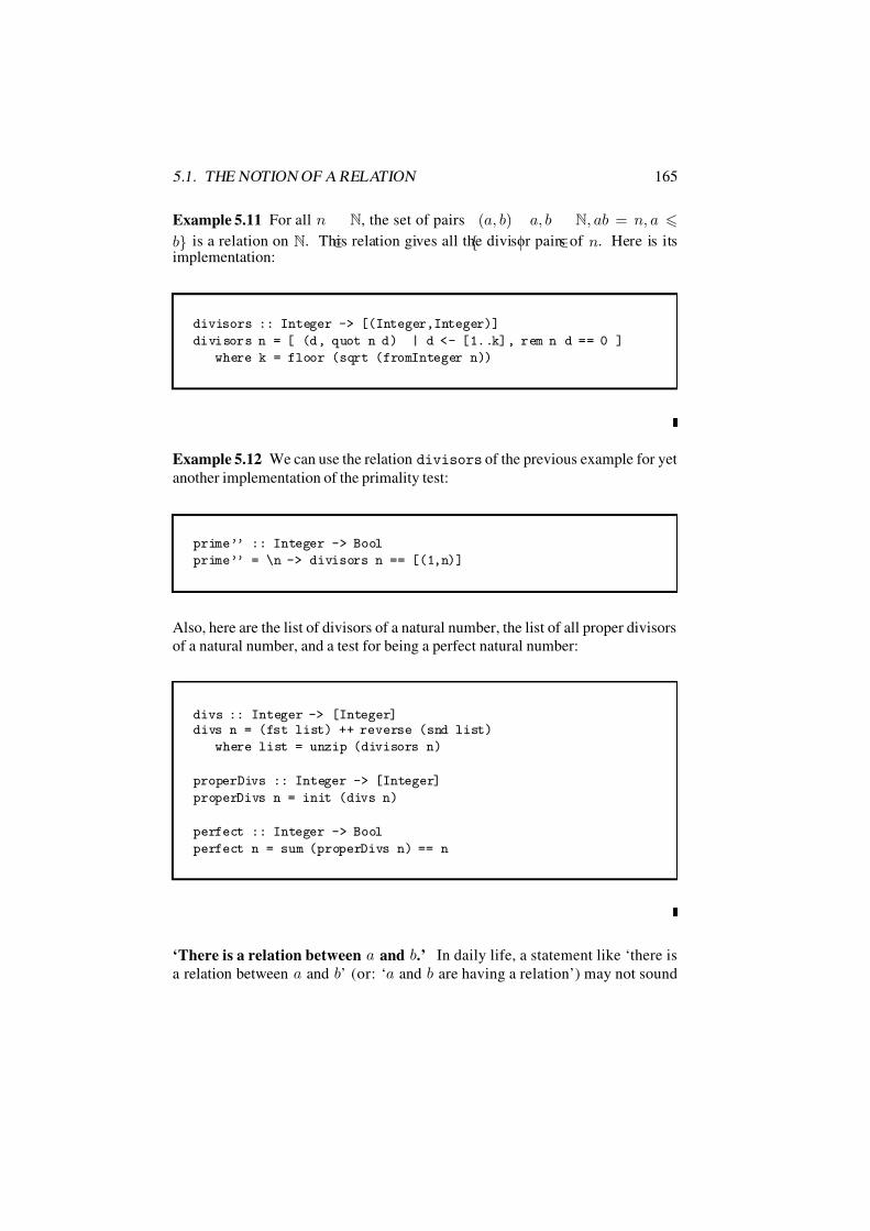
7/16/2019 The Haskell Road to Logic Maths and Programming
http://slidepdf.com/reader/full/the-haskell-road-to-logic-maths-and-programming-5634fa29ef7e9 176/448
5.1. THE NOTION OF A RELATION 165
Example 5.11 For all n
∈N, the set of pairs
(a, b)
|a, b
∈N, ab = n, a
b is a relation on N. This relation gives all the divisor pairs of n. Here is itsimplementation:
divisors :: Integer -> [(Integer,Integer)]
divisors n = [ (d, quot n d) | d <- [1..k], rem n d == 0 ]
where k = floor (sqrt (fromInteger n))
Example 5.12 We can use the relation divisors of the previous example for yet
another implementation of the primality test:
prime’’ :: Integer -> Bool
prime’’ = \n -> divisors n == [(1,n)]
Also, here are the list of divisors of a natural number, the list of all proper divisors
of a natural number, and a test for being a perfect natural number:
divs :: Integer -> [Integer]divs n = (fst list) ++ reverse (snd list)
where list = unzip (divisors n)
properDivs :: Integer -> [Integer]
properDivs n = init (divs n)
perfect :: Integer -> Bool
perfect n = sum (properDivs n) == n
‘There is a relation between a and b.’ In daily life, a statement like ‘there is
a relation between a and b’ (or: ‘a and b are having a relation’) may not sound

7/16/2019 The Haskell Road to Logic Maths and Programming
http://slidepdf.com/reader/full/the-haskell-road-to-logic-maths-and-programming-5634fa29ef7e9 177/448
166 CHAPTER 5. RELATIONS
unusual, but in the present context this should be avoided. Not because these are
false statements, but because they are so overly true, and, therefore, uninformative.Cf. Exercise 5.13. Of course, a statement like ‘ a stands in relation R to b’ or ‘the
relation R subsists between a and b’ can very well be informative, when R is some
specific relation.
Exercise 5.13 Show that ∀x∀y ∃R (xRy). (“Between every two things there exist
some relation.”)
In everyday situations, by saying that a and b are related we usually mean more
than that it is possible to form the ordered pair of a and b. We usually mean
that there is some good reason for considering the pair (a, b), because there is
some specific link between a and b (for instance, you can make Mrs. a blush by
mentioning Mr. b in conversation).
5.2 Properties of Relations
In this section we list some useful properties of relations on a set A. Further on,
in Sections 5.3 and 5.4, we will illustrate how tests for these properties can be
implemented.
A relation R is reflexive on A if for every x ∈ A: xRx.
Example 5.14 On any set A, the relation ∆A is reflexive. Note that ∆A is the
smallest reflexive relation on A: it is a subset of any reflexive relation on A. In
other words, a relation R is reflexive on A iff ∆A ⊆ R.
Example 5.15 The relation on N is reflexive (for every number is less than or
equal to itself).
A relation R on A is irreflexive if for no x ∈ A: xRx.
Example 5.16 The relation < on N is irreflexive.
Exercise 5.17 Show that a relation R on A is irreflexive iff ∆A ∩ R = ∅.
There are relations which are neither reflexive nor irreflexive (the reader is urged
to think up an example).
A relation R on A is symmetric if for all x, y ∈ A: if xRy then yRx.

7/16/2019 The Haskell Road to Logic Maths and Programming
http://slidepdf.com/reader/full/the-haskell-road-to-logic-maths-and-programming-5634fa29ef7e9 178/448
5.2. PROPERTIES OF RELATIONS 167
Example 5.18 The relation ‘having the same age’ between people is symmetric.
Unfortunately, the relation ‘being in love with’ between people is not symmetric.
Exercise 5.19 Show the following:
1. A relation R on a set A is symmetric iff ∀x, y ∈ A(xRy ⇔ yRx).
2. A relation R is symmetric iff R ⊆ R−1, iff R = R−1.
A relation R on A is asymmetric if for all x, y ∈ A: if xRy then not yRx.
The relation < on N is asymmetric. It is immediate from the definition that a
relation R on A is asymmetric iff R ∩ R−1 = ∅. Note that there are relationswhich are neither symmetric nor asymmetric.
Exercise 5.20 Show that every asymmetric relation is irreflexive.
A relation R on A is antisymmetric if for all x, y ∈ A: if xRy and yRx then
x = y.
Example 5.21 The relation m|n (m is a divisor of n) on N is antisymmetric. If mis a divisor of n and n is a divisor of m, then m and n are equal.
The relation in example 5.15 is antisymmetric.
Exercise 5.22 Show from the definitions that an asymmetric relation always isantisymmetric.
The converse of the statement in Exercise 5.22 is not true: the relation on N
provides a counterexample.
A relation R on A is transitive if for all x,y,z ∈ A: if xRy and yRz then xRz.
Examples of transitive relations are < and on N. If F is the relation ‘friendship’
on a set of people E , and every member of E endorses the laudable principle “The
friends of my friends are my friends”, then F is transitive.
Exercise 5.23 Show that a relation R on a set A is transitive iff
∀x, z ∈ A(∃y ∈ A(xRy ∧ yRz ) ⇒ xRz).

7/16/2019 The Haskell Road to Logic Maths and Programming
http://slidepdf.com/reader/full/the-haskell-road-to-logic-maths-and-programming-5634fa29ef7e9 179/448
168 CHAPTER 5. RELATIONS
A relation R on A is intransitive if for all x,y,z
∈A: if xRy and yRz then not
xRz.
Example 5.24 The relation ‘father of’ on the set of all human beings is intransi-
tive.
Again: there are relations that are neither transitive nor intransitive (think up an
example).
A relation R on A is a pre-order (or quasi-order) if R is transitive and reflexive.
Example 5.25 Let L be the set of all propositional formulas built from a given set
of atomic propositions. Then the relation |= given by
P |= Q iff P ⇒ Q is logically valid
is a pre-order on L. To check this, note that for every propositional formula P ,P ⇒ P is logically valid, so |= is reflexive. Also, for all propositional formulas
P,Q,R, if P ⇒ Q and Q ⇒ R are logically valid, then P ⇒ R is logically
valid. This can be checked as follows, by contraposition. Suppose P ⇒ R is not
logically valid. Then there is a valuation for the atomic propositions that makes P true and R false. Now there are two possibilities: this valuation makes Q true or
it makes Q false. If it makes Q true, then we know that Q ⇒ R is not logically
valid. If it makes Q false, then we know that P ⇒ Q is not logically valid. So
either P ⇒ Q or Q ⇒ R is not logically valid. This shows that |= is transitive.
Example 5.26 Let L be the set of all propositional formulas built from a given setof atomic propositions. Then the relation on L given by P Q iff there is a
proof of Q from the given P (this relation was defined in Chapter 3) is a pre-order.
See example 3.1 for the transitivity of . In fact, the relation coincides with
the relation |= of the previous example. The safety checks on the proof rules for
the logical connectives that were performed in Chapter 3 guarantee that ⊆ |=.
This fact is called the soundness of the proof system. The inclusion in the other
direction, |= ⊆ , is called the completeness of the proof system. It is outside the
scope of this book, but it is proved in [EFT94].
A relation R on A is a strict partial order if R is transitive and irreflexive. A
relation R on A is a partial order if R is transitive, reflexive and antisymmetric.
Note that the relation|= from example 5.25 is not antisymmetric. Take the formu-
las P ∧ Q and Q ∧ P . Then we have P ∧ Q |= Q ∧ P and Q ∧ P |= P ∧ Q, but
P ∧ Q and Q ∧ P are different formulas. Thus, |= is not a partial order.
7/16/2019 The Haskell Road to Logic Maths and Programming
http://slidepdf.com/reader/full/the-haskell-road-to-logic-maths-and-programming-5634fa29ef7e9 180/448
5.2. PROPERTIES OF RELATIONS 169
Example 5.27 The relation < on N is a strict partial order and the relation on
N is a partial order. Theorem 4.1 states that for any set A, the relation ⊆ on ℘(A)is a partial order.
Exercise 5.28 Show that every strict partial order is asymmetric.
Exercise 5.29 Show that every relation which is transitive and asymmetric is a
strict partial order.
Exercise 5.30 Show that if R is a strict partial order on A, then R∪∆A is a partial
order on A. (So every strict partial order is contained in a partial order.)
Exercise 5.31 Show that the inverse of a partial order is again a partial order.
A relation R on A is linear (or: has the comparison property) if for all x, y ∈ A:xRy or yRx or x = y. A partial order that is also linear is called a total order.
All Haskell types in class Ord a are total orders. A set A with a total order on it
is called a chain.
Exercise 5.32 Let S be a reflexive and symmetric relation on a set A.
A path is a finite sequence a1, . . . , an of elements of A such that for every i,
1 i < n, we have that aiSai+1. Such a path connects a1 with an.
Assume that for all a, b ∈ A there is exactly one path connecting a with b.
Fix r ∈ A. Define the relation on A by: a b iff a is one of the elements in the
path connecting r with b.
Show the following:
1. is reflexive,
2. is antisymmetric.
3. is transitive,
4. for all a ∈ A, r a,
5. for every a ∈ A, the set X a = x ∈ A | x a is finite and if b, c ∈ X athen b c or c b.
(A structure (A,, r) with these five properties is called a tree with root r. The
directory-structure of a computer account is an example of a tree. Another example
is the structure tree of a formula (see Section 2.3 above). These are examples of
finite trees, but if A is infinite, then the tree (A,, r) will have at least one infinite
branch.)

7/16/2019 The Haskell Road to Logic Maths and Programming
http://slidepdf.com/reader/full/the-haskell-road-to-logic-maths-and-programming-5634fa29ef7e9 181/448
170 CHAPTER 5. RELATIONS
Here is a list of all the relational properties of binary relations on a set A that we
discussed:
reflexivity ∀x xRx.
irreflexivity ∀x ¬xRx.
symmetry ∀xy (xRy ⇒ yRx).
asymmetry ∀xy (xRy ⇒ ¬yRx).
antisymmetry ∀xy (xRy ∧ yRx ⇒ x = y).
transitivity ∀xyz (xRy ∧ yRz ⇒ xRz).
intransitivity ∀xyz (xRy ∧ yRz ⇒ ¬xRz).
linearity ∀xy (xRy ∨ yRx ∨ x = y).
Because of their importance, relations that are transitive, reflexive and symmetric
(equivalence relations) deserve a section of their own (see Section 5.5).
irrefl refl asymm antisymm symm trans linear
pre-order√ √
strict partial order√ √ √ √
partial order√ √ √
total order√ √ √ √
equivalence√ √ √
Exercise 5.33 Consider the following relations on the natural numbers. Check
their properties (some answers can be found in the text above). The successor
relation is the relation given by (n, m) | n + 1 = m. The divisor relation
is (n, m) | n divides m. The coprime relation C on N is given by nCm :≡GCD(n, m) = 1, i.e., the only factor of n that divides m is 1, and vice versa (see
Section 8.2).
< successor divisor coprime
irreflexive
reflexive
asymmetric
antisymmetric
symmetric
transitive
linear
Definition 5.34 If O
is a set of properties of relations on a set A, then theO
-
closure of a relation R is the smallest relation S that includes R and that has all
the properties in O.
7/16/2019 The Haskell Road to Logic Maths and Programming
http://slidepdf.com/reader/full/the-haskell-road-to-logic-maths-and-programming-5634fa29ef7e9 182/448
5.2. PROPERTIES OF RELATIONS 171
The most important closures are the reflexive closure, the symmetric closure, the
transitive closure and the reflexive transitive closure of a relation.
Remark. To show that R is the smallest relation S that has all the properties in
O, show the following:
1. R has all the properties in O,
2. If S has all the properties in O, then R ⊆ S .
Exercise 5.35 Suppose that R is a relation on A.
1. Show that R ∪ ∆A is the reflexive closure of R.2. Show that R ∪ R−1 is the symmetric closure of R.
Exercise 5.36 Let R be a transitive binary relation on A. Does it follow from
the transitivity of R that its symmetric reflexive closure R ∪ R−1 ∪ ∆A is also
transitive? Give a proof if your answer is yes, a counterexample otherwise.
To define the transitive and reflexive transitive closures of a relation we need the
concept of relation composition.
Composing Relations. Suppose that R and S are relations on A. The composition
R S of R and S is the relation on A that is defined by
x(R S )z :≡ ∃y ∈ A(xRy ∧ ySz).
Furthermore, for n ∈ N, n 1 we define Rn by means of R1 := R, Rn+1 :=Rn R.
Example 5.37 In imperative programming, the meaning of a command can be
viewed as a relation on a set of machine states, where a machine state is a set of
pairs consisting of machine registers with their contents. If s = (r1, 4), (r2, 6), . . .then executing r2 := r1 in state s gives a new state s = (r1, 4), (r2, 4), . . ..
If C 1 and C 2 are commands, then we can execute them in sequential order as
C 1
; C 2
or as C 2
; C 1
. If the meaning of command C 1
is R and the meaning of
command C 2 is S , then the meaning of C 1; C 2 is R S and the meaning of C 2; C 1is S R.
7/16/2019 The Haskell Road to Logic Maths and Programming
http://slidepdf.com/reader/full/the-haskell-road-to-logic-maths-and-programming-5634fa29ef7e9 183/448
172 CHAPTER 5. RELATIONS
Exercise 5.38 Determine the composition of the relation “father of” with itself.
Determine the composition of the relations “brother of” and “parent of” Give anexample showing that R S = S R can be false.
Exercise 5.39 Consider the relation
R = (0, 2), (0, 3), (1, 0), (1, 3), (2, 0), (2, 3)
on the set A = 0, 1, 2, 3, 4.
1. Determine R2, R3 and R4.
2. Give a relation S on A such that R ∪ (S R) = S .
Exercise 5.40 Verify:
1. A relation R on A is transitive iff R R ⊆ R.
2. Give an example of a transitive relation R for which R R = R is false.
Exercise 5.41 Verify:
1. Q
(R
S ) = (Q
R)
S . (Thus, the notation Q
R
S is unambiguous.)
2. (R S )−1 = S −1 R−1.
We will show that for any relation R on A, the relation R+ =n1 Rn is the
transitive closure of R.
Because R = R1 ⊆ n1 Rn, we know that R ⊆ R+. We still have to prove
that R+ is transitive, and moreover that it is the smallest transitive relation that
contains R.
To see that R+ is transitive, assume xR+y and yR+z. From xR+y we get that
there is some k 1 with xRky. From yR+z we get that there is some m 1with yRmz. It follows that xRk+mz, and therefore xR+z, proving that R+ is
transitive.

7/16/2019 The Haskell Road to Logic Maths and Programming
http://slidepdf.com/reader/full/the-haskell-road-to-logic-maths-and-programming-5634fa29ef7e9 184/448
5.2. PROPERTIES OF RELATIONS 173
Proposition 5.42 R+ is the smallest transitive relation that contains R.
Proof. The proposition can be restated as follows. If T is a transitive relation on
A such that R ⊆ T , then R+ ⊆ T . We prove this fact by induction (see Chapter
7).
Basis If xRy then it follows from R ⊆ T that xT y.
Induction step Assume (induction hypothesis) that Rn ⊆ T . We have to show
that Rn+1 ⊆ T . Consider a pair (x, y) with xRn+1y. Then, by the definition
of Rn+1, there is a z such that xRnz and zRy . Because R ⊆ T we have
zT y, and the induction hypothesis yields xT z. By transitivity of T it now
follows that xT y.
Example 5.43 If A = a, b, c, then
a ∈+ A, b, c ∈+ A, b ∈+ A, c ∈+ A and c ∈+ A.
Example 5.44 On the set of human beings, the transitive closure of the ‘parent
of’ relation is the ‘ancestor of’ relation, and the transitive closure of the ‘child of’
relation is the ‘descendant of’ relation.
Exercise 5.45 Show that the relation < onN is the transitive closure of the relation
R = (n, n + 1) | n ∈ N.
Exercise 5.46 Let R be a relation on A. Show that R+ ∪ ∆A is the reflexive
transitive closure of R.
The reflexive transitive closure of a relation R is often called the ancestral of R,
notation R∗. Note that R∗ is a pre-order.
Exercise 5.47 Give the reflexive transitive closure of the following relation:
R = (n, n + 1) | n ∈ N.
Exercise 5.48*

7/16/2019 The Haskell Road to Logic Maths and Programming
http://slidepdf.com/reader/full/the-haskell-road-to-logic-maths-and-programming-5634fa29ef7e9 185/448
174 CHAPTER 5. RELATIONS
1. Show that an intersectionof arbitrarily many transitive relations is transitive.
2. Suppose that R is a relation on A. Note that A2 is one example of a transitive
relation on A that extends R. Conclude that the intersection of all transitive
relations extending R is the least transitive relation extending R. In other
words, R+ equals the intersection of all transitive relations extending R.
Exercise 5.49*
1. Show that (R∗)−1 = (R−1)∗.
2. Show by means of a counter-example that (R ∪ R−1)∗ = R∗ ∪ R−1∗ may
be false.
3. Prove: if S R ⊆ R S , then (R S )∗ ⊆ R∗ S ∗.
Exercise 5.50 Suppose that R and S are reflexive relations on the set A. Then
∆A ⊆ R and ∆A ⊆ S , so ∆A ⊆ R ∩ S , i.e., R ∩ S is reflexive as well. We say:
reflexivity is preserved under intersection. Similarly, if R and S are reflexive, then
∆A ⊆ R ∪ S , so R ∪ S is reflexive. Reflexivity is preserved under union. If Ris reflexive, then ∆A ⊆ R−1, so R−1 is reflexive. Reflexivity is preserved under
inverse. If R and S are reflexive, ∆A ⊆ R S , so R S is reflexive. Reflexivity is
preserved under composition. Finally, if R on A is reflexive, then the complement
of R, i.e., the relation A2
−R, is irreflexive. So reflexivity is not preserved under
complement. These closure properties of reflexive relations are listed in the tablebelow.
We can ask the same questions for other relational properties. Suppose R and
S are symmetric relations on A. Does it follow that R ∩ S is symmetric? That
R ∪ S is symmetric? That R−1 is symmetric? That A2 − R is symmetric? That
R S is symmetric? Similarly for the property of transitivity. These questions are
summarized in the table below. Complete the table by putting ‘yes’ or ‘no’ in the
appropriate places.
property reflexivity symmetry transitivity
preserved under ∩? yes ? ?
preserved under ∪? yes ? ?
preserved under inverse? yes ? ?preserved under complement? no ? ?
preserved under composition? yes ? ?
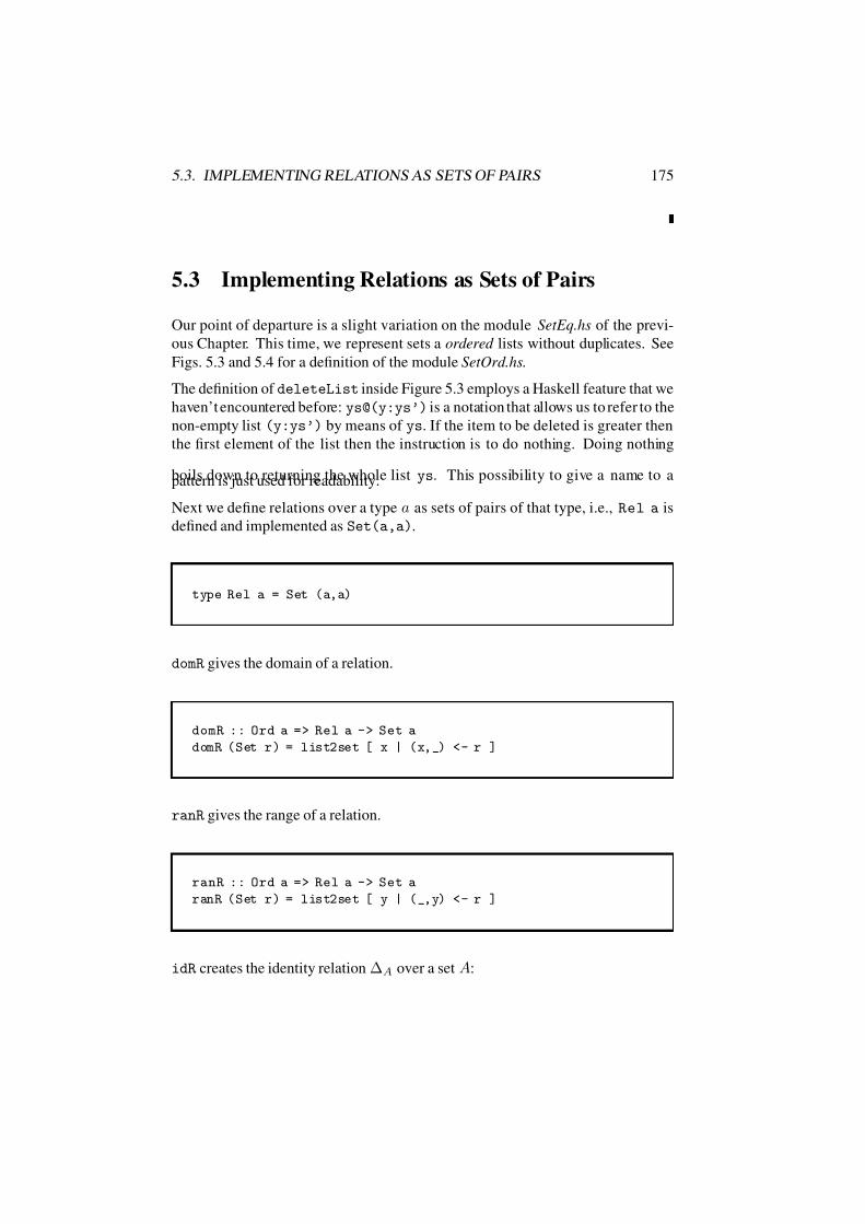
7/16/2019 The Haskell Road to Logic Maths and Programming
http://slidepdf.com/reader/full/the-haskell-road-to-logic-maths-and-programming-5634fa29ef7e9 186/448
5.3. IMPLEMENTING RELATIONS AS SETS OF PAIRS 175
5.3 Implementing Relations as Sets of Pairs
Our point of departure is a slight variation on the module SetEq.hs of the previ-
ous Chapter. This time, we represent sets a ordered lists without duplicates. See
Figs. 5.3 and 5.4 for a definition of the module SetOrd.hs.
The definition of deleteList inside Figure 5.3 employs a Haskell feature that we
haven’t encountered before: ys@(y:ys’) is a notation that allows us to refer to the
non-empty list (y:ys’) by means of ys. If the item to be deleted is greater then
the first element of the list then the instruction is to do nothing. Doing nothing
boils down to returning the whole list ys. This possibility to give a name to apattern is just used for readability.
Next we define relations over a type a as sets of pairs of that type, i.e., Rel a is
defined and implemented as Set(a,a).
type Rel a = Set (a,a)
domR gives the domain of a relation.
domR :: Ord a => Rel a -> Set a
domR (Set r) = list2set [ x | (x,_) <- r ]
ranR gives the range of a relation.
ranR :: Ord a => Rel a -> Set a
ranR (Set r) = list2set [ y | (_,y) <- r ]
idR creates the identity relation ∆A over a set A:
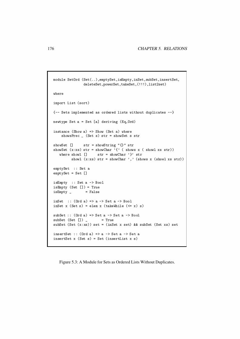
7/16/2019 The Haskell Road to Logic Maths and Programming
http://slidepdf.com/reader/full/the-haskell-road-to-logic-maths-and-programming-5634fa29ef7e9 187/448
176 CHAPTER 5. RELATIONS
module SetOrd (Set(..),emptySet,isEmpty,inSet,subSet,insertSet,
deleteSet,powerSet,takeSet,(!!!),list2set)
where
import List (sort)
-- Sets implemented as ordered lists without duplicates --
newtype Set a = Set [a] deriving (Eq,Ord)
instance (Show a) => Show (Set a) whereshowsPrec _ (Set s) str = showSet s str
showSet [] str = showString "" str
showSet (x:xs) str = showChar ’’ ( shows x ( showl xs str))
where showl [] str = showChar ’’ str
showl (x:xs) str = showChar ’,’ (shows x (showl xs str))
emptySet :: Set a
emptySet = Set []
isEmpty :: Set a -> Bool
isEmpty (Set []) = True
isEmpty _ = False
inSet :: (Ord a) => a -> Set a -> Bool
inSet x (Set s) = elem x (takeWhile (<= x) s)
subSet :: (Ord a) => Set a -> Set a -> Bool
subSet (Set []) _ = True
subSet (Set (x:xs)) set = (inSet x set) && subSet (Set xs) set
insertSet :: (Ord a) => a -> Set a -> Set a
insertSet x (Set s) = Set (insertList x s)
Figure 5.3: A Module for Sets as Ordered Lists Without Duplicates.
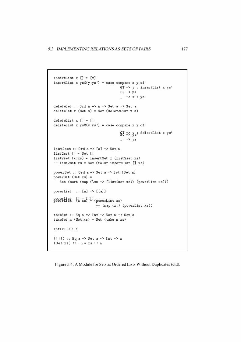
7/16/2019 The Haskell Road to Logic Maths and Programming
http://slidepdf.com/reader/full/the-haskell-road-to-logic-maths-and-programming-5634fa29ef7e9 188/448
5.3. IMPLEMENTING RELATIONS AS SETS OF PAIRS 177
insertList x [] = [x]
insertList x ys@(y:ys’) = case compare x y of
GT -> y : insertList x ys’
EQ -> ys
_ -> x : ys
deleteSet :: Ord a => a -> Set a -> Set a
deleteSet x (Set s) = Set (deleteList x s)
deleteList x [] = []
deleteList x ys@(y:ys’) = case compare x y of
GT -> y : deleteList x ys’EQ -> ys’
_ -> ys
list2set :: Ord a => [a] -> Set a
list2set [] = Set []
list2set (x:xs) = insertSet x (list2set xs)
-- list2set xs = Set (foldr insertList [] xs)
powerSet :: Ord a => Set a -> Set (Set a)
powerSet (Set xs) =
Set (sort (map (\xs -> (list2set xs)) (powerList xs)))
powerList :: [a] -> [[a]]
powerList [] = [[]]powerList (x:xs) = (powerList xs)
++ (map (x:) (powerList xs))
takeSet :: Eq a => Int -> Set a -> Set a
takeSet n (Set xs) = Set (take n xs)
infixl 9 !!!
(!!!) :: Eq a => Set a -> Int -> a
(Set xs) !!! n = xs !! n
Figure 5.4: A Module for Sets as Ordered Lists Without Duplicates (ctd).
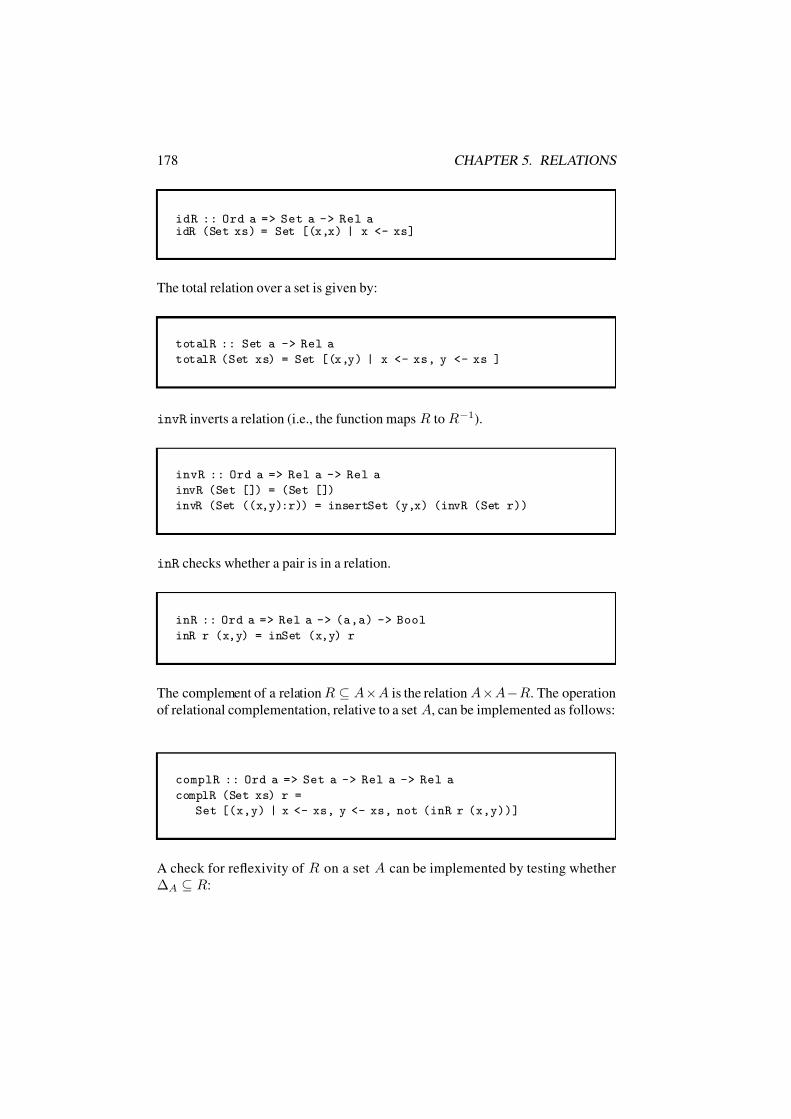
7/16/2019 The Haskell Road to Logic Maths and Programming
http://slidepdf.com/reader/full/the-haskell-road-to-logic-maths-and-programming-5634fa29ef7e9 189/448
178 CHAPTER 5. RELATIONS
idR :: Ord a => Set a -> Rel aidR (Set xs) = Set [(x,x) | x <- xs]
The total relation over a set is given by:
totalR :: Set a -> Rel a
totalR (Set xs) = Set [(x,y) | x <- xs, y <- xs ]
invR inverts a relation (i.e., the function maps R to R−1).
invR :: Ord a => Rel a -> Rel a
invR (Set []) = (Set [])
invR (Set ((x,y):r)) = insertSet (y,x) (invR (Set r))
inR checks whether a pair is in a relation.
inR :: Ord a => Rel a -> (a,a) -> Bool
inR r (x,y) = inSet (x,y) r
The complement of a relation R ⊆ A×A is the relation A×A−R. The operation
of relational complementation, relative to a set A, can be implemented as follows:
complR :: Ord a => Set a -> Rel a -> Rel a
complR (Set xs) r =
Set [(x,y) | x <- xs, y <- xs, not (inR r (x,y))]
A check for reflexivity of R on a set A can be implemented by testing whether
∆A ⊆ R:
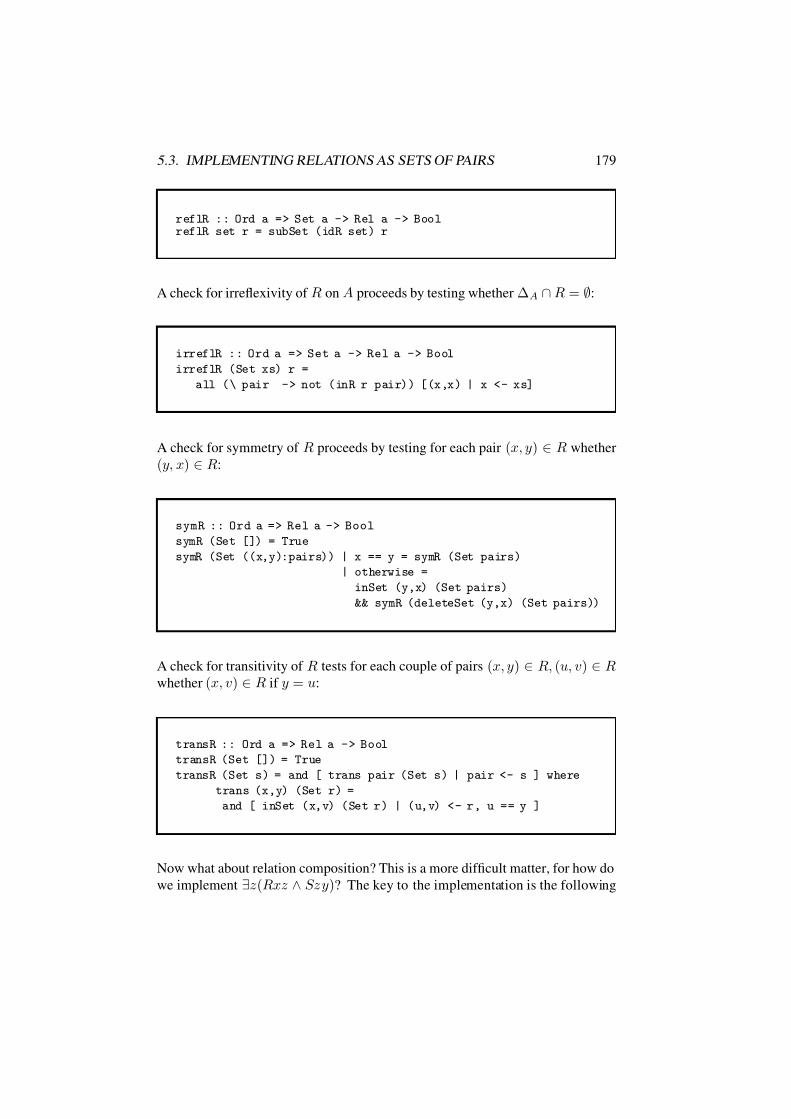
7/16/2019 The Haskell Road to Logic Maths and Programming
http://slidepdf.com/reader/full/the-haskell-road-to-logic-maths-and-programming-5634fa29ef7e9 190/448
5.3. IMPLEMENTING RELATIONS AS SETS OF PAIRS 179
reflR :: Ord a => Set a -> Rel a -> BoolreflR set r = subSet (idR set) r
A check for irreflexivity of R on A proceeds by testing whether ∆A ∩ R = ∅:
irreflR :: Ord a => Set a -> Rel a -> Bool
irreflR (Set xs) r =
all (\ pair -> not (inR r pair)) [(x,x) | x <- xs]
A check for symmetry of R proceeds by testing for each pair (x, y) ∈ R whether
(y, x) ∈ R:
symR :: Ord a => Rel a -> Bool
symR (Set []) = True
symR (Set ((x,y):pairs)) | x == y = symR (Set pairs)
| otherwise =
inSet (y,x) (Set pairs)
&& symR (deleteSet (y,x) (Set pairs))
A check for transitivity of R tests for each couple of pairs (x, y) ∈ R, (u, v) ∈ Rwhether (x, v) ∈ R if y = u:
transR :: Ord a => Rel a -> Bool
transR (Set []) = True
transR (Set s) = and [ trans pair (Set s) | pair <- s ] where
trans (x,y) (Set r) =
and [ inSet (x,v) (Set r) | (u,v) <- r, u == y ]
Now what about relation composition? This is a more difficult matter, for how do
we implement ∃z(Rxz ∧ Sz y)? The key to the implementation is the following

7/16/2019 The Haskell Road to Logic Maths and Programming
http://slidepdf.com/reader/full/the-haskell-road-to-logic-maths-and-programming-5634fa29ef7e9 191/448
180 CHAPTER 5. RELATIONS
procedure for composing a single pair of objects (x, y) with a relation S , simply
by forming the relation (x, z) | (z, y) ∈ S . This is done by:
composePair :: Ord a => (a,a) -> Rel a -> Rel a
composePair (x,y) (Set []) = Set []
composePair (x,y) (Set ((u,v):s))
| y == u = insertSet (x,v) (composePair (x,y) (Set s))
| otherwise = composePair (x,y) (Set s)
For relation composition we need set union (Cf. Exercise 4.54):
unionSet :: (Ord a) => Set a -> Set a -> Set a
unionSet (Set []) set2 = set2
unionSet (Set (x:xs)) set2 =
insertSet x (unionSet (Set xs) (deleteSet x set2))
Relation composition is defined in terms of composePair and unionSet:
compR :: Ord a => Rel a -> Rel a -> Rel a
compR (Set []) _ = (Set [])compR (Set ((x,y):s)) r =
unionSet (composePair (x,y) r) (compR (Set s) r)
Composition of a relation with itself (Rn):
repeatR :: Ord a => Rel a -> Int -> Rel a
repeatR r n | n < 1 = error "argument < 1"
| n == 1 = r
| otherwise = compR r (repeatR r (n-1))

7/16/2019 The Haskell Road to Logic Maths and Programming
http://slidepdf.com/reader/full/the-haskell-road-to-logic-maths-and-programming-5634fa29ef7e9 192/448
5.3. IMPLEMENTING RELATIONS AS SETS OF PAIRS 181
Example 5.51 Let us use the implementation to illustrate Exercise 5.39.
r = Set [(0,2),(0,3),(1,0),(1,3),(2,0),(2,3)]
r2 = compR r r
r3 = repeatR r 3
r4 = repeatR r 4
This gives:
REL> r
(0,2),(0,3),(1,0),(1,3),(2,0),(2,3)REL> r2
(0,0),(0,3),(1,2),(1,3),(2,2),(2,3)
REL> r3
(0,2),(0,3),(1,0),(1,3),(2,0),(2,3)
REL> r4
(0,0),(0,3),(1,2),(1,3),(2,2),(2,3)
REL> r == r2
False
REL> r == r3
True
REL> r == r4
False
REL> r2 == r4
True
Also, the following test yields ‘True’:
s = Set [(0,0),(0,2),(0,3),(1,0),(1,2),(1,3),(2,0),(2,2),(2,3)]
test = (unionSet r (compR s r)) == s
Exercise 5.52 Extend this implementation with a function
restrictR :: Ord a => Set a -> Rel a -> Rel a
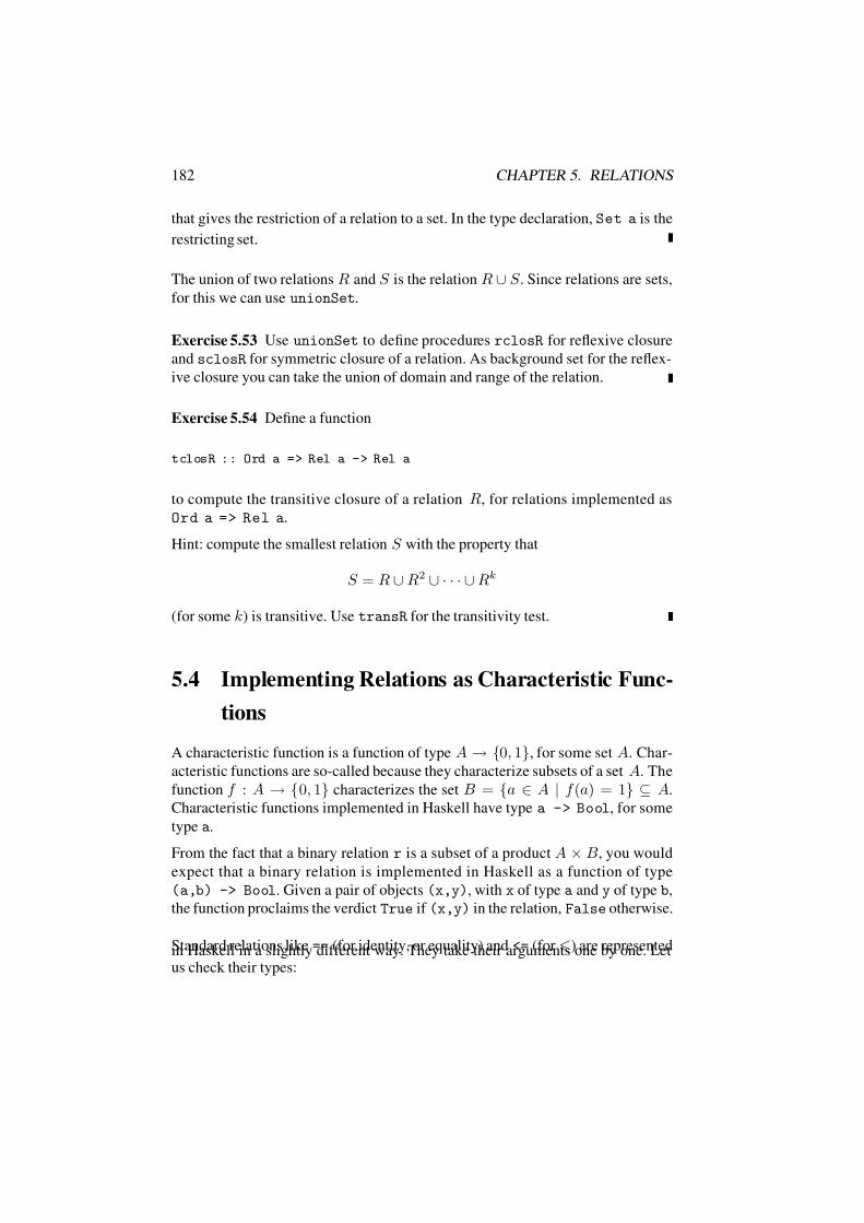
7/16/2019 The Haskell Road to Logic Maths and Programming
http://slidepdf.com/reader/full/the-haskell-road-to-logic-maths-and-programming-5634fa29ef7e9 193/448
182 CHAPTER 5. RELATIONS
that gives the restriction of a relation to a set. In the type declaration, Set a is the
restricting set.
The union of two relations R and S is the relation R ∪ S . Since relations are sets,
for this we can use unionSet.
Exercise 5.53 Use unionSet to define procedures rclosR for reflexive closure
and sclosR for symmetric closure of a relation. As background set for the reflex-
ive closure you can take the union of domain and range of the relation.
Exercise 5.54 Define a function
tclosR :: Ord a => Rel a -> Rel a
to compute the transitive closure of a relation R, for relations implemented as
Ord a => Rel a.
Hint: compute the smallest relation S with the property that
S = R ∪ R2 ∪ · · · ∪ Rk
(for some k) is transitive. Use transR for the transitivity test.
5.4 Implementing Relations as Characteristic Func-
tions
A characteristic function is a function of type A → 0, 1, for some set A. Char-
acteristic functions are so-called because they characterize subsets of a set A. The
function f : A → 0, 1 characterizes the set B = a ∈ A | f (a) = 1 ⊆ A.
Characteristic functions implemented in Haskell have type a -> Bool, for some
type a.
From the fact that a binary relation r is a subset of a product A × B, you would
expect that a binary relation is implemented in Haskell as a function of type
(a,b) -> Bool. Given a pair of objects (x,y), with x of type a and y of type b,
the function proclaims the verdict True if (x,y) in the relation, False otherwise.
Standard relations like == (for identity, or equality) and <= (for ) are representedin Haskell in a slightly different way. They take their arguments one by one. Letus check their types:
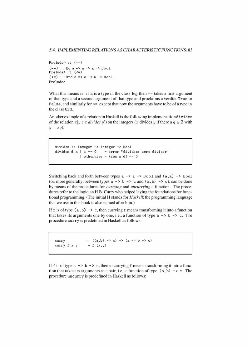
7/16/2019 The Haskell Road to Logic Maths and Programming
http://slidepdf.com/reader/full/the-haskell-road-to-logic-maths-and-programming-5634fa29ef7e9 194/448
5.4. IMPLEMENTING RELATIONS AS CHARACTERISTIC FUNCTIONS183
Prelude> :t (==)
(==) :: Eq a => a -> a -> BoolPrelude> :t (<=)
(<=) :: Ord a => a -> a -> Bool
Prelude>
What this means is: if a is a type in the class Eq , then == takes a first argument
of that type and a second argument of that type and proclaims a verdict True or
False, and similarly for <=, except that now the arguments have to be of a type in
the class Ord.
Another example of a relation in Haskell is the following implementationdivides
of the relation x|y (‘x divides y’) on the integers (x divides y if there a q ∈ Z with
y = xq ).
divides :: Integer -> Integer -> Bool
divides d n | d == 0 = error "divides: zero divisor"
| otherwise = (rem n d) == 0
Switching back and forth between types a -> a -> Bool and (a,a) -> Bool
(or, more generally, between types a - > b - > c and (a,b) -> c), can be done
by means of the procedures for currying and uncurrying a function. The proce-
dures refer to the logician H.B. Curry who helped laying the foundations for func-
tional programming. (The initial H stands for Haskell; the programming language
that we use in this book is also named after him.)
If f is of type (a,b) -> c, then currying f means transforming it into a function
that takes its arguments one by one, i.e., a function of type a - > b - > c. The
procedure curry is predefined in Haskell as follows:
curry :: ((a,b) -> c) -> (a -> b -> c)
curry f x y = f (x,y)
If f is of type a - > b - > c, then uncurrying f means transforming it into a func-
tion that takes its arguments as a pair, i.e., a function of type (a,b) -> c. The
procedure uncurry is predefined in Haskell as follows:
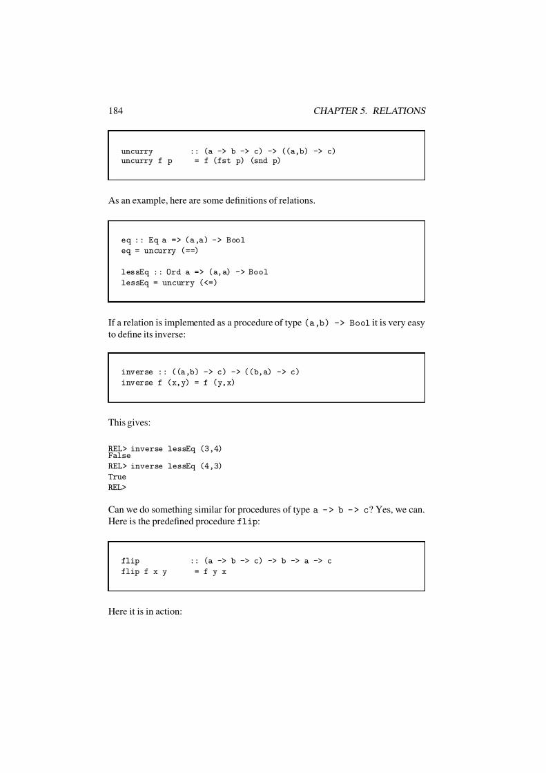
7/16/2019 The Haskell Road to Logic Maths and Programming
http://slidepdf.com/reader/full/the-haskell-road-to-logic-maths-and-programming-5634fa29ef7e9 195/448
184 CHAPTER 5. RELATIONS
uncurry :: (a -> b -> c) -> ((a,b) -> c)uncurry f p = f (fst p) (snd p)
As an example, here are some definitions of relations.
eq :: Eq a => (a,a) -> Bool
eq = uncurry (==)
lessEq :: Ord a => (a,a) -> Bool
lessEq = uncurry (<=)
If a relation is implemented as a procedure of type (a,b) -> Bool it is very easy
to define its inverse:
inverse :: ((a,b) -> c) -> ((b,a) -> c)
inverse f (x,y) = f (y,x)
This gives:
REL> inverse lessEq (3,4)False
REL> inverse lessEq (4,3)
True
REL>
Can we do something similar for procedures of type a - > b - > c? Yes, we can.
Here is the predefined procedure flip:
flip :: (a -> b -> c) -> b -> a -> c
flip f x y = f y x
Here it is in action:

7/16/2019 The Haskell Road to Logic Maths and Programming
http://slidepdf.com/reader/full/the-haskell-road-to-logic-maths-and-programming-5634fa29ef7e9 196/448
5.4. IMPLEMENTING RELATIONS AS CHARACTERISTIC FUNCTIONS185
REL> flip (<=) 3 4
FalseREL> flip (<=) 4 3
True
REL>
The procedure flip can be used to define properties from relations. Take the
property of dividing the number 102. This denotes the set
d ∈ N+ | d divides 102 = 1, 2, 3, 6, 17, 34, 51, 102.
It is given in Haskell by (‘divides‘ 102), which in turn is shorthand for
flip divides 102
Trying this out, we get:
REL> filter (‘divides‘ 102) [1..300]
[1,2,3,6,17,34,51,102]
We will now work out the representation of relations as characteristic functions.
To keep the code compatible with the implementation given before, we define the
type as Rel’, and similarly for the operations.
type Rel’ a = a -> a -> Bool
emptyR’ :: Rel’ a
emptyR’ = \ _ _ -> False
list2rel’ :: Eq a => [(a,a)] -> Rel’ a
list2rel’ xys = \ x y -> elem (x,y) xys
idR’ creates the identity relation over a list.
idR’ :: Eq a => [a] -> Rel’ a
idR’ xs = \ x y -> x == y && elem x xs
invR’ inverts a relation.

7/16/2019 The Haskell Road to Logic Maths and Programming
http://slidepdf.com/reader/full/the-haskell-road-to-logic-maths-and-programming-5634fa29ef7e9 197/448
186 CHAPTER 5. RELATIONS
invR’ :: Rel’ a -> Rel’ ainvR’ = flip
inR’ checks whether a pair is in a relation.
inR’ :: Rel’ a -> (a,a) -> Bool
inR’ = uncurry
Checks whether a relation is reflexive, irreflexive, symmetric or transitive (on a
domain given by a list):
reflR’ :: [a] -> Rel’ a -> Bool
reflR’ xs r = and [ r x x | x <- xs ]
irreflR’ :: [a] -> Rel’ a -> Bool
irreflR’ xs r = and [ not (r x x) | x <- xs ]
symR’ :: [a] -> Rel’ a -> Bool
symR’ xs r = and [ not (r x y && not (r y x)) | x <- xs, y <- xs ]
transR’ :: [a] -> Rel’ a -> Bool
transR’ xs r = and
[ not (r x y && r y z && not (r x z))
| x <- xs, y <- xs, z <- xs ]
Union, intersection, reflexive and symmetric closure of relations:

7/16/2019 The Haskell Road to Logic Maths and Programming
http://slidepdf.com/reader/full/the-haskell-road-to-logic-maths-and-programming-5634fa29ef7e9 198/448
5.4. IMPLEMENTING RELATIONS AS CHARACTERISTIC FUNCTIONS187
unionR’ :: Rel’ a -> Rel’ a -> Rel’ aunionR’ r s x y = r x y || s x y
intersR’ :: Rel’ a -> Rel’ a -> Rel’ a
intersR’ r s x y = r x y && s x y
reflClosure’ :: Eq a => Rel’ a -> Rel’ a
reflClosure’ r = unionR’ r (==)
symClosure’ :: Rel’ a -> Rel’ a
symClosure’ r = unionR’ r (invR’ r)
Relation composition:
compR’ :: [a] -> Rel’ a -> Rel’ a -> Rel’ a
c o m p R ’ x s r s x y = o r [ r x z & & s z y | z < - x s ]
Composition of a relation with itself:
repeatR’ :: [a] -> Rel’ a -> Int -> Rel’ a
repeatR’ xs r n | n < 1 = error "argument < 1"| n == 1 = r
| otherwise = compR’ xs r (repeatR’ xs r (n-1))
Exercise 5.55 Use the implementation of relations Rel’ a as characteristic func-tions over type a to define an example relation r with the property that
unionR r (compR r r)
is not the transitive closure of r.
Exercise 5.56 If a relation r :: Rel’ a is restricted to a finite list xs, then wecan calculate the transitive closure of r restricted to the list xs. Define a function

7/16/2019 The Haskell Road to Logic Maths and Programming
http://slidepdf.com/reader/full/the-haskell-road-to-logic-maths-and-programming-5634fa29ef7e9 199/448
188 CHAPTER 5. RELATIONS
transClosure’ :: [a] -> Rel’ a -> Rel’ a
for this.
Hint: compute the smallest relation S with the property that
S = R ∪ R2 ∪ · · · ∪ Rk
(for some k) is transitive. Use transR xs for the transitivity test on domain xs.
5.5 Equivalence Relations
Definition 5.57 A relation R on A is an equivalence relation or equivalence if
R is transitive, reflexive on A and symmetric.
Example 5.58 On the set of human beings the relation of having the same age is
an equivalence relation.
Example 5.59 The relation R = (n, m) | n, m ∈ N and n + m is even is an
equivalence relation on N.
The equivalence test can be implemented for relations of type Ord a => Rel a
as follows:
equivalenceR :: Ord a => Set a -> Rel a -> BoolequivalenceR set r = reflR set r && symR r && transR r
For relations implemented as type Rel’ a the implementation goes like this:
equivalenceR’ :: [a] -> Rel’ a -> Bool
equivalenceR’ xs r = reflR’ xs r && symR’ xs r && transR’ xs r
Example 5.60 The next table shows for a number of familiar relations whether
they have the properties of reflexivity, symmetry and transitivity. Here:

7/16/2019 The Haskell Road to Logic Maths and Programming
http://slidepdf.com/reader/full/the-haskell-road-to-logic-maths-and-programming-5634fa29ef7e9 200/448
5.5. EQUIVALENCE RELATIONS 189
• ∅is the empty relation on N,
• ∆ = ∆N = (n, n) | n ∈ N is the identity on N,
• N2 = N× N is the biggest relation on N,
• < and are the usual ordering relations on N,
• Suc is the relation on N defined by Suc(n, m) ≡ n + 1 = m,
• ⊆ is the inclusion relation on ℘(N).
property: yes: no:
reflexive (on N resp. ℘(N)) ∆, N2, , ⊆ ∅, <, Suc
symmetric∅
, ∆, N2 <, , Suc,⊆transitive ∅, ∆, N2, <, , ⊆ Suc
The table shows that among these examples only ∆ andN2 are equivalences onN.
Example 5.61 The relation ∅ is (trivially) symmetric and transitive. The relation
∅ is reflexive on the set ∅, but on no other set. Thus: ∅ is an equivalence on the set
∅, but on no other set.
Example 5.62 Let A be a set. ∆A is the smallest equivalence on A. A2 is the
biggest equivalence on A.
Example 5.63 The relation ∼ between vectors in 3-dimensional space R3 that is
defined by a ∼ b ≡ ∃r ∈ R+ (a = r b) is an equivalence.
Example 5.64 For any n ∈ Z, n = 0, the relation ≡n on Z is given by m ≡n kiff m and k have the same remainder when divided by n. More precisely, m ≡n k(or: m ≡ k (mod n)) iff
• m = qn + r, with 0 r < n,
• k = q n + r, with 0 r < n ,
• r = r.
When m ≡n k we say that m is equivalent to k modulo n. The relation ≡n is also
called the (mod n) relation.

7/16/2019 The Haskell Road to Logic Maths and Programming
http://slidepdf.com/reader/full/the-haskell-road-to-logic-maths-and-programming-5634fa29ef7e9 201/448
190 CHAPTER 5. RELATIONS
To show that
≡n from Example 5.64 is an equivalence, the following proposition
is useful.
Proposition 5.65 m ≡n k iff n | m − k.
Proof. ⇒: Suppose m ≡n k. Then m = qn + r and k = q n + r with 0 r < nand 0 r < n and r = r. Thus, m−k = (q −q )n, and it follows that n | m−k.
⇐: Suppose n | m − k. Then n | (qn + r) − (q n + r), so n | r − r. Since
−n < r − r < n, this implies r − r = 0, so r = r. It follows that m ≡n k.
From this we get that the following are all equivalent:
• m ≡n k.
• n | m − k.
• ∃a ∈ Z : an = m − k.
• ∃a ∈ Z : m = k + an.
• ∃a ∈ Z : k = m + an.
Exercise 5.66 Show that for every n ∈ Z with n = 0 it holds that ≡n is an
equivalence on Z.
Example 5.67 Here is a Haskell implementation of the modulo relation:
modulo :: Integer -> Integer -> Integer -> Bool
modulo n = \ x y -> divides n (x-y)
Example 5.68 The relation that applies to two finite sets in case they have the
same number of elements is an equivalence on the collection of all finite sets.
The corresponding equivalence on finite lists is given by the following piece of
Haskell code:

7/16/2019 The Haskell Road to Logic Maths and Programming
http://slidepdf.com/reader/full/the-haskell-road-to-logic-maths-and-programming-5634fa29ef7e9 202/448
5.5. EQUIVALENCE RELATIONS 191
equalSize :: [a] -> [b] -> BoolequalSize list1 list2 = (length list1) == (length list2)
Abstract equivalences are often denoted by ∼ or ≈.
Exercise 5.69 Determine whether the following relations on N are (i) reflexive on
N, (ii) symmetric, (iii) transitive:
1. (2, 3), (3, 5), (5, 2);
2. (n, m) | |n − m| 3.
Exercise 5.70 A = 1, 2, 3. Can you guess how many relations there are on this
small set? Indeed, there must be sufficiently many to provide for the following
questions.
1. Give an example of a relation on A that is reflexive, but not symmetric and
not transitive.
2. Give an example of a relation on A that is symmetric, but not reflexive and
not transitive.
3. Give examples (if any) of relations on A that satisfy each of the six remain-
ing possibilities w.r.t. reflexivity, symmetry and transitivity.
Exercise 5.71 For finite sets A (0, 1, 2, 3, 4 and 5 elements and n elements gener-
ally) the following table has entries for: the number of elements in A2, the number
of elements in ℘(A2) (that is: the number of relations on A), the number of rela-
tions on A that are (i) reflexive, (ii) symmetric and (iii) transitive, and the number
of equivalences on A.

7/16/2019 The Haskell Road to Logic Maths and Programming
http://slidepdf.com/reader/full/the-haskell-road-to-logic-maths-and-programming-5634fa29ef7e9 203/448

7/16/2019 The Haskell Road to Logic Maths and Programming
http://slidepdf.com/reader/full/the-haskell-road-to-logic-maths-and-programming-5634fa29ef7e9 204/448
5.6. EQUIVALENCE CLASSES AND PARTITIONS 193
Example 5.77 (continued from example 5.63) The equivalence class of (1, 1, 1)
∈R3 modulo ∼ is the set (r,r,r) | r > 0: half a straight line starting at the origin(not including the origin). (A “direction”.)
Example 5.78 (continued from example 5.67) The equivalence class of 2 in Z
(mod 4) is the set
. . . , −6, −2, 2, 6, 10, 14, . . . = 2 + 4n | n ∈ Z .
The implementation yields:
REL> filter (modulo 4 2) [-15..15]
[-14,-10,-6,-2,2,6,10,14]
Example 5.79 (continued from example 5.68) The equivalence class of 0, 1, 2modulo the equivalence of having the same number of elements is the collection
of all three-element sets.
*(According to the Frege-Russell defi nition of natural number, this is the number three.)
Lemma 5.80 Suppose that R is an equivalence on A. If a, b ∈ A , then:
| a |R = | b |R ⇔ aRb.
Proof. ⇒ : Note that a ∈ | a |R (for, R is reflexive). Thus, if | a |R = | b |R, then
a ∈ | b |R, i.e., aRb.
⇐ : Assume that aRb. Then also bRa (R is symmetric.)
|a
|R
⊆ |b|R: x
∈ |a
|R signifies xRa, and hence xRb follows (R transitive);
therefore, x ∈ | b |R.
| b |R ⊆ | a |R: similarly.
Extensionality completes the proof.
Lemma 5.81 Let R be an equivalence on A.
1. Every equivalence class is non-empty,
2. every element of A belongs to some equivalence class,
3. different equivalence classes are disjoint.
Proof. 1/2. Since R is reflexive on A, we have, for every a ∈ A: a ∈ | a |.3. Suppose that
|a|
and|
b|
are not disjoint. Say, c∈ |
a| ∩ |
b|. Then we have both
cRa and cRb. Since R is symmetric, it follows that aRc. Thus, aRb (R transitive).
Therefore, | a | = | b | follows, using Lemma 5.80.

7/16/2019 The Haskell Road to Logic Maths and Programming
http://slidepdf.com/reader/full/the-haskell-road-to-logic-maths-and-programming-5634fa29ef7e9 205/448
194 CHAPTER 5. RELATIONS
Exercise 5.82 Use the implementation of relations Rel’ a as characteristic func-
tions over type a to implement a function raccess that takes a relation r, an objectx, and a list L, and returns the list of all objects y from L such that rxy holds. Thetype declaration should run:
raccess :: Rel’ a -> a -> [a] -> [a]
The concept of partitioning a set is made precise in the following definition.
Definition 5.83 A family A of subsets of a set A is called a partition of A if
• ∅/
∈ A,
• A = A,
• for all X, Y ∈ A: if X = Y then X ∩ Y = ∅.
The elements of a partition are called its components.
This definition says that every element of A is in some member of A and that no
element of A is in more than one member of A.
Example 5.84 1, 2, 3, 4 is a partition of 1, 2, 3, 4. ∅ (trivially) is a parti-
tion of ∅. Z can be partitioned into the negative integers, the positive integers, and
0.
Exercise 5.85 Show the following: if Ai | i ∈ I is a partition of A and Bj | j ∈ J is a partition of B, then Ai× Bj | (i, j) ∈ I × J is a partition of A × B.
Definition 5.86 (Quotients) Assume that R is an equivalence on the set A. The
collection of equivalence classes of R, A/R = | a | | a ∈ A, is called the
quotient of A modulo R.
The definition of partition was engineered in order to ensure the following:
Theorem 5.87 Every quotient (of a set, modulo an equivalence) is a partition (of
that set).
Proof. This is nothing but a reformulation of Lemma 5.81.

7/16/2019 The Haskell Road to Logic Maths and Programming
http://slidepdf.com/reader/full/the-haskell-road-to-logic-maths-and-programming-5634fa29ef7e9 206/448
5.6. EQUIVALENCE CLASSES AND PARTITIONS 195
Example 5.88 (continued from examples 5.62 and 5.76)
A/∆A = a | a ∈ A .
A/A2 = A.
Example 5.89 (continued from examples 5.63 and 5.77)
The partition R3/∼ of R3 has components 0 and all half-lines.
Example 5.90 (continued from examples 5.67 and 5.78)
The partition Z/mod(4) of Z induced by the equivalence mod(4) has four com-
ponents: (i) the equivalence class 4n | n ∈ Z of 0 (that also is the equivalence
class of 4, 8, 12,...,−4. . . ), (ii) the class 4n + 1 | n ∈ Z of 1, (iii) the class
4n + 2 | n ∈ Z of 2, and (iv) 4n + 3 | n ∈ Z, the class of 3. The quotient
Z/mod(n) is usually written as Zn.
Example 5.91*(continued from examples 5.68 and 5.79)
The quotient of the collection of finite sets modulo the relation “same number of
elements” is —according to Frege and Russell— the set of natural numbers.
Exercise 5.92 Give the partition that the relation of example 5.59 induces on N.
Example 5.93 (continued from Example 5.72)
Let R be a pre-order on A. Then ∼ given by x ∼ y :≡ xRy ∧ yRx is an equiva-
lence relation. Consider the relation R∼ on A/∼ given by |x|R∼|y| :≡ xRy. The
relation R∼ is a partial order on A/∼ called the po-set reflection of R.
The definition is independent of the representatives, because assume x ∼ x andy ∼ y and xRy. Then xRx ∧ xRx, yRy ∧ yRy, and xRy. From xRx, xRyand yRy by transitivity of R, xRy.
R∼ is reflexive, because R is. R∼ is anti-symmetric, for suppose |x|R∼|y| and
|y|R∼|x|. Then xRy and yRx, so by definition of ∼, |x| = |y|. Finally R∼ is
transitive because R is.
Thus, equivalences induce partitions. But the process can be inverted.
Theorem 5.94 Every partition (of a set) is a quotient (of that set, modulo a certain
equivalence).
Specifically: Suppose thatA
is a partition of A. Then the relation R on A defined
by
xRy :≡ ∃K ∈A (x, y ∈ K )

7/16/2019 The Haskell Road to Logic Maths and Programming
http://slidepdf.com/reader/full/the-haskell-road-to-logic-maths-and-programming-5634fa29ef7e9 207/448
196 CHAPTER 5. RELATIONS
(x and y member of the same component of
A) is an equivalence on A, and
Ais
the collection of equivalence classes of R.
Proof. Exercise 5.121.
According to Theorems 5.87 and 5.94, equivalences and partitions are two sides
of the same coin.
Example 5.95 Consider the following relation on 0, 1, 2, 3, 4:
(0, 0), (0, 1), (1, 0), (1, 1), (2, 2), (2, 4), (3, 3), (4, 2), (4, 4).
This is an equivalence, and the corresponding partition is
0, 1, 2, 4, 3.
Exercise 5.96 Is the following relation an equivalence on 0, 1, 2, 3, 4? If so,
give the corresponding partition.
(0, 0), (0, 3), (0, 4), (1, 1), (1, 2),(2, 1), (2, 2), (3, 0), (3, 3), (3, 4), (4, 0), (4, 3), (4, 4).
Example 5.97 The equivalence corresponding to the partition
0, 1, 2, 3, 4of 0, 1, 2, 3, 4 is:
(0, 0), (1, 1), (1, 2), (1, 3), (2, 1), (2, 2), (2, 3), (3, 1), (3, 2), (3, 3), (4, 4).
Exercise 5.98 What are the equivalences corresponding to the following parti-
tions?:
1. 0, 3, 1, 2, 4, of 0, 1, 2, 3, 4,
2. n ∈ Z | n < 0, 0, n ∈ Z | n > 0, of Z,
3. even numbers, odd numbers, of N.

7/16/2019 The Haskell Road to Logic Maths and Programming
http://slidepdf.com/reader/full/the-haskell-road-to-logic-maths-and-programming-5634fa29ef7e9 208/448
5.6. EQUIVALENCE CLASSES AND PARTITIONS 197
Exercise 5.99 A = 1, 2, 3, 4, 5,
R = (1, 1), (1, 2), (1, 4), (2, 1), (2, 2), (2, 4),(3, 3), (3, 5), (4, 1), (4, 2), (4, 4), (5, 3), (5, 5).
1. Is R an equivalence on A? If so, answer 2 and 3:
2. Determine |2|R.
3. Determine A/R.
Example 5.100 If ∼ on ℘(N) is given by
A ∼ B :≡ (A − B) ∪ (B − A) is finite,
then ∼ is reflexive. If A ⊆ N is arbitrary, then (A − A) ∪ (A − A) = ∅ ∪ ∅ = ∅,
and ∅ is finite.
Exercise 5.101* Define the relation ∼ on ℘(N) by:
A ∼ B :≡ (A − B) ∪ (B − A) is finite.
Thus, N ∼ ∅, since (N− ∅) ∪ (∅ −N) = N ∪ ∅ = N is infinite.
Show that
∼is an equivalence (reflexivity is shown in example 5.100).
Exercise 5.102 Define the relation R on all people by: aRb :≡ a and b have a
common ancestor. Is R transitive?
Same question for the relation S defined by: aSb :≡ a and b have a common
ancestor along the male line.
Example 5.103 For counting the partitions of a set A of size n, the key is to count
the number of ways of partitioning a set A of size n into k non-empty classes.
Let us usenk
for this number, and see if we can find a recurrence for it, i.e., an
equation in terms of the function for smaller arguments. Distributing n objects
over 1 set can be done in only one way, so
n1
= 1. Similarly, distributing n
objects over n non-empty sets can be done in only one way, so nn = 1.
To distribute n objects over k different sets, we can either (i) put the last object
into an equivalence class of its own, or (ii) put it in one of the existing classes.

7/16/2019 The Haskell Road to Logic Maths and Programming
http://slidepdf.com/reader/full/the-haskell-road-to-logic-maths-and-programming-5634fa29ef7e9 209/448
198 CHAPTER 5. RELATIONS
(i) can be done in n−1k
−1 ways, for this is the number of ways to distribute n
−1
objects over k − 1 non-empty classes. (ii) can be done in k · n−1k ways, for there
are k classes to choose from, andn−1k
ways to distribute n − 1 objects over k
classes. Thus, the recurrence we need is:n
k
= k ·
n − 1
k
+
n − 1
k − 1
.
In terms of this, the number of partitions b(n) is given by:
b(n) =nk=1
n
k
.
The numbers nk are called Stirling set numbers. The b(n) are called Bell num-
bers.
Exercise 5.104 Implement functions bell and stirling to count the number of
different partitions of a set of n elements.
Exercise 5.105 Use the result of Exercise 5.104 to fill out the last column in the
table of Exercise 5.71 on p. 191.
Exercise 5.106 Show: conditions 2 and 3 of Definition 5.83 taken together are
equivalent with: for every a ∈ A there exists exactly one K ∈ A such that a ∈ K .
Exercise 5.107 Is the intersection R
∩S of two equivalences R and S on a set A
again an equivalence? And the union R ∪ S ? Prove, or supply a simple counter-example. (See the table of Exercise 5.50.)
Exercise 5.108* Suppose that R and S are equivalences on A such that R ⊆ S .Show that every S -equivalence class is a union of R-equivalence classes.
Exercise 5.109 A list partition is the list counterpart of a partition: list partitions
are of type Eq a => [[a]], and a list partition xss of xs has the following prop-
erties:
• [] is not an element of xss,
• xs and concat xss have the same elements,
• if ys and zs are distinct elements of xss, then ys and zs have no elements
in common.
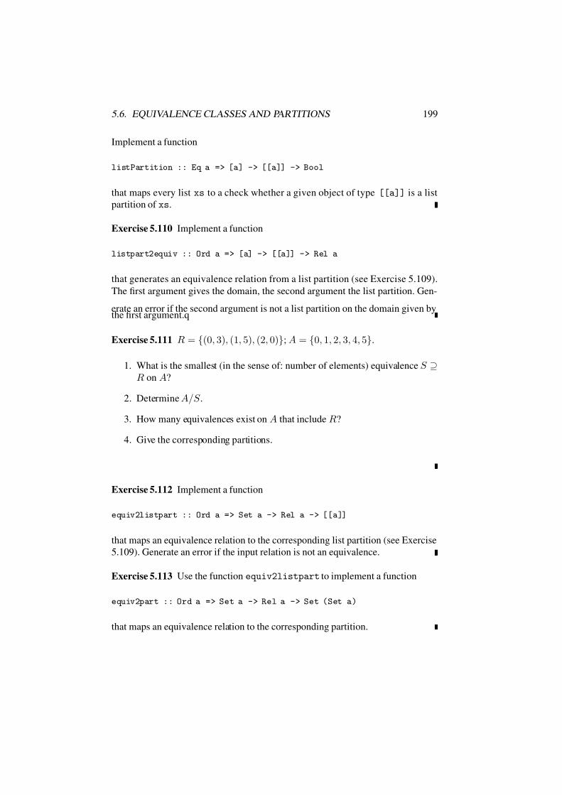
7/16/2019 The Haskell Road to Logic Maths and Programming
http://slidepdf.com/reader/full/the-haskell-road-to-logic-maths-and-programming-5634fa29ef7e9 210/448
5.6. EQUIVALENCE CLASSES AND PARTITIONS 199
Implement a function
listPartition :: Eq a => [a] -> [[a]] -> Bool
that maps every list xs to a check whether a given object of type [[a]] is a list
partition of xs.
Exercise 5.110 Implement a function
listpart2equiv :: Ord a => [a] -> [[a]] -> Rel a
that generates an equivalence relation from a list partition (see Exercise 5.109).
The first argument gives the domain, the second argument the list partition. Gen-
erate an error if the second argument is not a list partition on the domain given bythe first argument.q
Exercise 5.111 R = (0, 3), (1, 5), (2, 0); A = 0, 1, 2, 3, 4, 5.
1. What is the smallest (in the sense of: number of elements) equivalence S ⊇R on A?
2. Determine A/S .
3. How many equivalences exist on A that include R?
4. Give the corresponding partitions.
Exercise 5.112 Implement a function
equiv2listpart :: Ord a => Set a -> Rel a -> [[a]]
that maps an equivalence relation to the corresponding list partition (see Exercise
5.109). Generate an error if the input relation is not an equivalence.
Exercise 5.113 Use the function equiv2listpart to implement a function
equiv2part :: Ord a => Set a -> Rel a -> Set (Set a)
that maps an equivalence relation to the corresponding partition.

7/16/2019 The Haskell Road to Logic Maths and Programming
http://slidepdf.com/reader/full/the-haskell-road-to-logic-maths-and-programming-5634fa29ef7e9 211/448
200 CHAPTER 5. RELATIONS
Exercise 5.114* R is a relation on A. One of the following is the smallest equiva-
lence on A that includes R. Which? Prove.
1. (∆A ∪ R)+ ∪ (∆A ∪ R−1)+.
2. ∆A ∪ R+ ∪ (R−1)+.
3. ∆A ∪ (R ∪ R−1)+.
Exercise 5.115 Let R be a relation on A. Show that S = R∗ ∩ R−1∗ is an
equivalence on A. Next, show that the relation T on the quotient A/S given by
|a|S T |b|S :≡ aR∗b is a partial order.
Note that the reasoning of Exercise 5.115 only uses reflexivity and transitivity of
R∗. So, in general, if R is a reflexive transitive relation on A (i.e., R is a pre-order),
then S = R ∩R−1 is an equivalence on A, and the relation T on the quotient A/S given by |a|S T |b|S :≡ aRb is a partial order.
Example 5.116 Consider the pre-order |= of Example 5.25. Note that the equiva-
lence relation |= ∩ |=−1 is nothing other than the relation ≡ of logical equivalence.
Remark. In constructions with quotients, it often happens that a relation on the
quotient is defined in terms of a relation on the underlying set. In such a case one
should always check that the definition is proper in the sense that it is independent
of the representatives that are mentioned in it.Take again the example of exercise 5.115, of a set A with a reflexive transitive
relation R on it. If S = R ∩ R−1, then the definition of relation T on the quotient
A/S given by |a|S T |b|S :≡ aRb is proper, because it holds that aRb, a ∈ |a|S and b ∈ |b|S together imply that aRb.
To see that this is so, assume a ∈ |a|S and aRb. Then aSa, so aRa, and by
transitivity of R, aRb. Suppose b ∈ |b|S . Then bSb, so bRb. Together with
aRb this gives, again by transitivity of R, that aRb.
Exercise 5.117 Define the relations ∼ and ≈ on R by p ∼ q :≡ p × q ∈ Z,
p ≈ q :≡ p − q ∈ Z. Are these equivalences? If so, describe the corresponding
partition(s).
Exercise 5.118 Define the relation R on R × R by (x, y)R(u, v) iff 3x − y =3u − v.

7/16/2019 The Haskell Road to Logic Maths and Programming
http://slidepdf.com/reader/full/the-haskell-road-to-logic-maths-and-programming-5634fa29ef7e9 212/448
5.6. EQUIVALENCE CLASSES AND PARTITIONS 201
1. Show that R is an equivalence.
2. Describe the equivalence classes of (0, 0) and (1, 1).
3. DescribeR×R/R in geometrical terms.
Exercise 5.119 Define an equivalence on R × R that partitions the plane in con-
centric circles with (0, 0) as centre.
Exercise 5.120 Q = (0, 0), (0, 1), (0, 5), (2, 4), (5, 0). For an equivalence Ron 0, 1, 2, 3, 4, 5 it is given, that Q ⊆ R and (0, 2) /∈ R.
1. Show that (1, 5) ∈ R and (4, 5) ∈ R.
2. Give the partition corresponding to the smallest (in the sense of number of
elements) equivalence ⊇ Q.
3. How many equivalences S are there on 0, 1, 2, 3, 4, 5 such that Q ⊆ S and (0, 2) ∈ S ? Give the corresponding partitions.
Exercise 5.121 Prove Theorem 5.94.
Hint. Make sure that you use all properties of partitions.
Exercise 5.122* On a certain planet there are 20 countries. Every two of themeither are at war with each other or have a peace treaty. Every two countries with
a common enemy have such a peace treaty. What is the least possible number of
peace treaties on this planet?
Hint: Note that the relations P and W , for being at peace and at war, respectively,
exclude one another, that they are both irreflexive and symmetric, and that they
satisfy the principle that there are no war-triangles. For if x is at war with both yand z, then y and z have x as common enemy, hence y and z have a peace treaty:
∀xyz((xW y ∧ xW z) ⇒ yP z).
Find a recurrence (see page 212) for the maximum number of countries at war
among 2n countries. Next, use this to derive the minimum number of peace treaties
among 2n countries.

7/16/2019 The Haskell Road to Logic Maths and Programming
http://slidepdf.com/reader/full/the-haskell-road-to-logic-maths-and-programming-5634fa29ef7e9 213/448
202 CHAPTER 5. RELATIONS
5.7 Integer Partitions
Integer partitions of n ∈ N+ are lists of non-zero natural numbers that add up to
exactly n. For example, the four integer partitions of 4 are
[4], [1, 3], [2, 2], [1, 1, 2], [1, 1, 1, 1].
The integer partitions of n correspond to the sizes of the set partitions of a set Awith |A| = n. Here is an algorithm for generating integer partitions, in lexico-
graphically decreasing order:
• The first integer partition of n is [n].
• Let B be the last integer partition generated. If B consists of only 1’s, then
done. Otherwise, there is a smallest non-1 part m. To generate the next
partition, subtract 1 from m and collect all the units so as to match the new
smallest part m − 1.
Examples The partition after [1, 1, 3, 3] is [1, 2, 2, 3], for after subtracting 1 from
3, we should pack the three units that result in parcels of size 2. The partition after
[1, 1, 1, 1, 1, 1, 5] is [3, 4, 4], for after subtracting 1 from 5, we should pack the
seven units that result in parcels with maximum size 4, which gives three units and
one parcel of size 4, which in turn gives one parcel of size 3 and one of size 4. The
partition after [3, 3, 5] is [1, 2, 3, 5]. The partition after [1, 3, 3, 4] is [2, 2, 3, 4].
Implementation An integer partition is represented as a list of integers. For
convenience we count the number of 1’s, and remove them from the partition.
This gives a compressed representation (2, [3, 3]) of [1, 1, 3, 3]. These compressed
partitions have type CmprPart.
type Part = [Int]
type CmprPart = (Int,Part)
Expansion of a compressed partition (n, p) is done by generating n 1’s followed
by p:

7/16/2019 The Haskell Road to Logic Maths and Programming
http://slidepdf.com/reader/full/the-haskell-road-to-logic-maths-and-programming-5634fa29ef7e9 214/448
5.7. INTEGER PARTITIONS 203
expand :: CmprPart -> Partexpand (0,p) = p
expand (n,p) = 1:(expand ((n-1),p))
In generating the next partition from (k,xs) we may assume that xs is non-empty,
and that its elements are listed in increasing order.
The partition that follows (k,x:xs) is generated by packing (k+x,x:xs) for
maximum size x − 1. This assumes that x is the smallest element in x:xs.
nextpartition :: CmprPart -> CmprPart
nextpartition (k,(x:xs)) = pack (x-1) ((k+x),xs)
To pack a partition (m,xs) for size 1, there is nothing to do. To pack a partition
(m,xs) for maximum size k > 1 and k > m, decrease the parcel size to k − 1.
To pack a partition (m,xs) for size k > 1 and k m, use k units to generate one
parcel of size k, and go on with (m-k,k:xs), for the same parcel size.
pack :: Int -> CmprPart -> CmprPart
pack 1 (m,xs) = (m,xs)
pack k (m,xs) = if k > m then pack (k-1) (m,xs)
else pack k (m-k,k:xs)
To generate all partitions starting from a given partition (n,[]), just list the par-
tition consisting of n units, for this is the last partition. To generate all partitions
starting from a given partition (n,x:xs), list this partition, and then generate from
the successor of (n,x:xs).
generatePs :: CmprPart -> [Part]
generatePs p@(n,[]) = [expand p]
generatePs p@(n,(x:xs)) =
(expand p: generatePs(nextpartition p))

7/16/2019 The Haskell Road to Logic Maths and Programming
http://slidepdf.com/reader/full/the-haskell-road-to-logic-maths-and-programming-5634fa29ef7e9 215/448
204 CHAPTER 5. RELATIONS
Generate all partitions starting from [n]. The case where n = 1 is special, for it
is the only case where the compressed form of the first partition has a non-zeronumber of units.
part :: Int -> [Part]
part n | n < 1 = error "part: argument <= 0"
| n == 1 = [[1]]
| otherwise = generatePs (0,[n])
Here is what we get out:
REL> part 5[[5],[1,4],[2,3],[1,1,3],[1,2,2],[1,1,1,2],[1,1,1,1,1]]
REL> part 6
[[6],[1,5],[2,4],[1,1,4],[3,3],[1,2,3],[1,1,1,3],[2,2,2],
[1,1,2,2],[1,1,1,1,2],[1,1,1,1,1,1]]
REL> length (part 20)
627
Exercise 5.123 Write a program change :: Int -> [Int] that returns change
in EURO coins for any positive integer, in the least number of coins. Measure the
values of the EURO coins 0.01, 0.02, 0.05, 0.10, 0.20, 0.50, 1, 2 in EURO cents,
as 1, 2, 5, 10, 20, 50, 100, 200. Use pack for inspiration.
Exercise 5.124 Modify the integer partition algorithm so that it generates all thepossible ways of giving coin change for amounts of money up to 10 EURO, using
all available EURO coins (0.01, 0.02, 0.05, 0.10, 0.20, 0.50, 1, 2). Measure the
values of the EURO coins in EURO cents, as 1, 2, 5, 10, 20, 50, 100, 200.
Exercise 5.125 How many different ways are there to give change for one EURO?
Use the program from the previous exercise.
5.8 Further Reading
More on relations in the context of set theory in [DvDdS78]. Binary relations on
finite sets are studied in graph theory. See Chapters 4 and 5 of [Bal91]. Relationsin the context of database theory are the topic of [AHV95].

7/16/2019 The Haskell Road to Logic Maths and Programming
http://slidepdf.com/reader/full/the-haskell-road-to-logic-maths-and-programming-5634fa29ef7e9 216/448
Chapter 6
Functions
Preview
In mathematics, the concept of a function is perhaps even more important than that
of a set. Also, functions are crucial in computer programming, as the functional
programming paradigm demonstrates. This chapter introduces basic notions and
then moves on to special functions, operations on functions, defining equivalences
by means of functions, and compatibility of equivalences with operations.
Many concepts from the abstract theory of functions translate directly into compu-tational practice. Most of the example functions mentioned in this chapter can be
implemented directly in Haskell by just keying in their definitions, with domains
and co-domains specified as Haskell types.
Still, we have to bear in mind that an implementation of a function as a com-
puter program is a concrete incarnation of an abstract object. The same func-
tion may be computed by vastly different computation procedures. If you key
in sum [2*k | k <- [1 .. 100] ] at the hugs prompt you get the answer
10100, and if you key in 100 * 101 you get the same answer, but the compu-
tation steps that are performed to get at the answers are different. We have already
seen that there is no mechanical test for checking whether two procedures perform
the same task (Section 4.2), although in particular cases such results can be proved
by mathematical induction (see Chapter 7). E.g., in Example 7.4 in Chapter 7 it
is proved by mathematical induction that the computational recipesn
k=1 2k and
n(n + 1) specify the same function.
205

7/16/2019 The Haskell Road to Logic Maths and Programming
http://slidepdf.com/reader/full/the-haskell-road-to-logic-maths-and-programming-5634fa29ef7e9 217/448
206 CHAPTER 6. FUNCTIONS
module FCT
where
import List
6.1 Basic Notions
A function is something that transforms an object given to it into another one. The
objects that can be given to a function are called its arguments, and the results of the transformation are called values. The set of arguments is called the domain of
the function. We say that a function is defined on its domain.
If f is a function and x one of its arguments, then the corresponding value is
denoted by f (x). A function value y = f (x) is called the image of x under f .That f (x) = y can also be indicated by f : x −→ y. The domain of f is denoted
by dom (f ). Its range is ran(f ) = f (x) | x ∈ dom (f ).
Example 6.1 A function can be given as a rule or a prescription how to carry out
the transformation.
• First square, next add one is the function that transforms a real x ∈ R into
x2 + 1.
Letting f stand for this function, it is customary to describe it by the equation
f (x) = x2 + 1.
The Haskell implementation uses the same equation:
f x = x ^ 2 + 1
• The function described by
|x| =
x if x 0−x if x < 0

7/16/2019 The Haskell Road to Logic Maths and Programming
http://slidepdf.com/reader/full/the-haskell-road-to-logic-maths-and-programming-5634fa29ef7e9 218/448
6.1. BASIC NOTIONS 207
transforms a real into its absolute value. The Haskell implementation given
in Prelude.hs follows this definition to the letter:
absReal x | x >= 0 = x
| otherwise = -x
• The identity function 1A defined on A does not “transform” at all in the
usual sense of the word: given an argument x ∈ A, it outputs x itself. A
polymorphic identity function is predefined in Haskell as follows:
id :: a -> a
i d x = x
Set theory has the following simple definition of the concept of a function.
Definition 6.2 A function is a relation f that satisfies the following condition.
(x, y)
∈f
∧(x, z)
∈f =
⇒y = z.
That is: for every x ∈ dom (f ) there is exactly one y ∈ ran(f ) such that (x, y) ∈f .
If x ∈ dom (f ), then f (x) is by definition the unique object y ∈ ran(f ) for which
(x, y) ∈ f .
Note that we use dom here in the sense defined for relations, but that the relation
and the function-sense of the notion coincide: the domain dom (f ) of the function
f is x | ∃y((x, y) ∈ f ); exactly as in the relation-case (cf. Definition 5.1 p. 162).
Similarly, the range of f coincides with the range of f as a relation.
The set-theoretic and the computational view on functions are worlds apart, for
computationally a function is an algorithm for computing values. However, in
cases of functions with finite domains it is easy to switch back and forth between
the two perspectives, as the following conversions demonstrate.

7/16/2019 The Haskell Road to Logic Maths and Programming
http://slidepdf.com/reader/full/the-haskell-road-to-logic-maths-and-programming-5634fa29ef7e9 219/448
208 CHAPTER 6. FUNCTIONS
list2fct :: Eq a => [(a,b)] -> a -> blist2fct [] _ = error "function not total"
list2fct ((u,v):uvs) x | x == u = v
| otherwise = list2fct uvs x
fct2list :: (a -> b) -> [a] -> [(a,b)]
fct2list f xs = [ (x, f x) | x <- xs ]
The range of a function, implemented as a list of pairs, is given by:
ranPairs :: Eq b => [(a,b)] -> [b]ranPairs f = nub [ y | (_,y) <- f ]
If a function is defined on an enumerable domain, we can list its (finite or infinite)
range starting from a given element.
listValues :: Enum a => (a -> b) -> a -> [b]
listValues f i = (f i) : listValues f (succ i)
If we also know that the domain is bounded, we can generate the whole range as a
finite list.
listRange :: (Bounded a, Enum a) => (a -> b) -> [b]
listRange f = [ f i | i <- [minBound..maxBound] ]
Example 6.3
• The function x → x2 +1 defined onR is identified with the relation(x, y) |x ∈ R ∧ y = x2 + 1 = (x, x2 + 1) | x ∈ R.

7/16/2019 The Haskell Road to Logic Maths and Programming
http://slidepdf.com/reader/full/the-haskell-road-to-logic-maths-and-programming-5634fa29ef7e9 220/448
6.1. BASIC NOTIONS 209
•f =
(1, 4), (2, 4), (3, 6)
is a function. dom (f ) =
1, 2, 3
, ran(f ) =
4, 6.
• (1, 4), (2, 4), (2, 6) is not a function.
• ∆X , the identity-relation on X (Definition 5.7, p. 163), also is a function
from X to X . When viewed as a function, the identity relation on X is
usually written as 1X .
• If f is a function, we clearly have that f = (a, f (a)) | a ∈ dom (f ), and
ran(f ) = f (a) | a ∈ dom (f ).
• The relation ∅ is a function. dom (∅) = ∅ = ran(∅).
As is the case for relations, functions are more often given in a context of two sets.
Compare 5.3 (p. 162).
Definition 6.4 (From . . . to, On, Co-domain) Suppose that X and Y are sets. A
function f is from X to Y ; notation:
f : X −→ Y,
if dom (f ) = X and ran(f ) ⊆ Y . (Note the difference in terminology compared
with 5.3!)
In this situation, Y is called the co-domain of f .
A function f is said to be defined on X if dom (f ) = X .
Note that the set-theoretic way of identifying the function f with the relation R =(x, f (x)) | x ∈ X has no way of dealing with this situation: it is not possible to
recover the intended co-domain Y from the relation R. As far as R is concerned,
the co-domain of f could be any set that extends ran(R).
More Than One Argument. Functions as introduced here are unary, i.e., they
apply to only one argument. But of course, functions with more than one argument
(binary, ternary. . . ) do exist. E.g., addition and multiplication on N are of this
kind. However, such a binary (ternary.. . ) function can be viewed as a unary one
that applies to ordered pairs (resp., triples.. . ).
As we have seen, Haskell has predefined operations curry and uncurry to switch
back and forth between functions of types (a,b) -> c and a - > b - > c. We

7/16/2019 The Haskell Road to Logic Maths and Programming
http://slidepdf.com/reader/full/the-haskell-road-to-logic-maths-and-programming-5634fa29ef7e9 221/448
210 CHAPTER 6. FUNCTIONS
can extend this to cases of functionsthat take triples, quadruples, etc. as arguments.
As an example, here is the case for currying functions that take triples to functionsthat take three arguments, and for uncurrying functions that take three arguments
to functions that take triples.
curry3 :: ((a,b,c) -> d) -> a -> b -> c -> d
curry3 f x y z = f (x,y,z)
uncurry3 :: (a -> b -> c -> d) -> (a,b,c) -> d
uncurry3 f (x,y,z) = f x y z
Fact 6.5 (Function Equality) If f and g are functions that share their domain(dom (f ) = dom (g)) and, on it, carry out the same transformation (i.e., ∀x ∈dom (f )(f (x) = g(x))), then — according to Extensionality 4.1, p. 115 — we
have that f = g.
To establish that two functions f, g : X → Y are different we have to find an
x ∈ X with f (x) = g(x). As we have seen in Section 4.2, there is no generic
algorithm for checking function equality. Therefore, to establish that two functions
f, g : X → Y are equal, we need a proof. The general form, spelled out in full, of
such a proof is:
Given: f, g : X → Y .To be proved: f = g.
Proof:
Let x be an arbitrary object in X .
To be proved: f (x) = g(x).
Proof:
. . .
Thus f (x) = g(x).
Thus f = g.
Example 6.6 If f and g are defined on R by f (x) = x2 + 2x + 1, resp., g(x) =(x + 1)2, then f = g. Thus, functions are not distinguished by the details of how
they actually transform (in this respect, f and g differ), but only with respect to
their output-behaviour.

7/16/2019 The Haskell Road to Logic Maths and Programming
http://slidepdf.com/reader/full/the-haskell-road-to-logic-maths-and-programming-5634fa29ef7e9 222/448
6.1. BASIC NOTIONS 211
Warning. If functions f : X
→Y and g : X
→Z are given in the domain-
co-domain-context, and ∀x ∈ X (f (x) = g(x)), then f and g count as equal onlyif we also have that Y = Z . The co-domains are taken as an integral part of the
functions.
Function Definitions. If t(x) is an expression that describes an element of Y in terms of an element x ∈ X , then we can define a function f : X −→ Y by
writing:
Let the function f : X → Y be defined by f (x) = t(x).
For completely specifying a function f three things are sufficient:
• Specify dom (f ),
• Specify the co-domain of f ,
• Give an instruction for how to construct f (x) from x.
Examples of such instructions are x → x + 1, x → x2, and in fact all the Haskell
definitions of functions that we have encountered in this book.
A very convenient notation for function construction is by means of lambda ab-straction (page 58). In this notation, λx.x+1 encodes the specification x → x+1.The lambda operator is a variable binder, so λx.x+1 and λy.y +1 denote the samefunction. In fact, every time we specify a function foo in Haskell by means of
f o o x y z = t
we can think of this as a specification λxyz.t. If the types of x , y , z , t are known,
this also specifies a domain and a co-domain. For if x : : a, y : : b, z : : c,
t : : d, then λxyz.t has type a - > b - > c - > d.
Example 6.7
1. t(x) is the expression 2x2 + 3:
Let the function g : R −→ R be defined by g(x) = 2x2 + 3.
2. t(x) is the expression
x
0y sin(y)dy:
Let the function h : R−→
R be defined by h(x) = x0 y sin(y) dy.
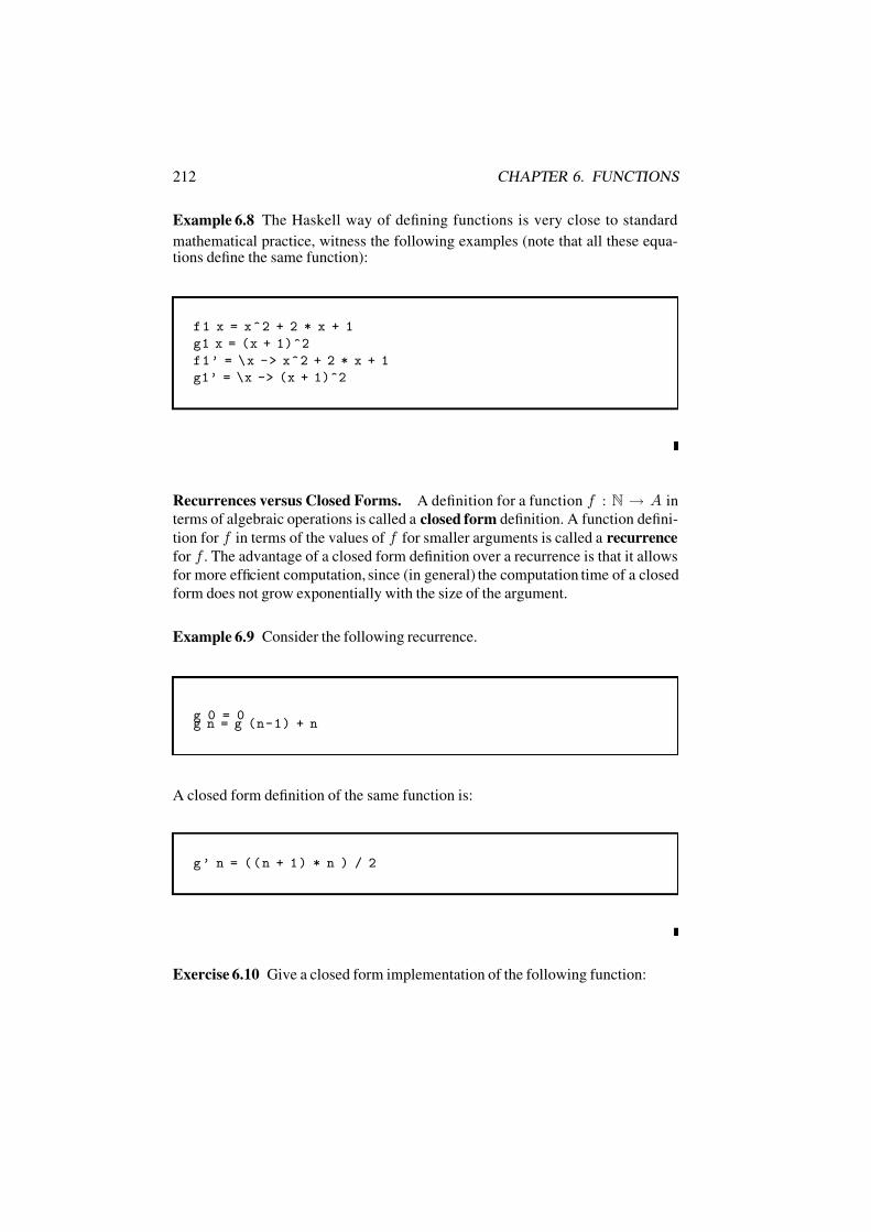
7/16/2019 The Haskell Road to Logic Maths and Programming
http://slidepdf.com/reader/full/the-haskell-road-to-logic-maths-and-programming-5634fa29ef7e9 223/448
212 CHAPTER 6. FUNCTIONS
Example 6.8 The Haskell way of defining functions is very close to standard
mathematical practice, witness the following examples (note that all these equa-tions define the same function):
f 1 x = x ^ 2 + 2 * x + 1
g1 x = (x + 1)^2
f 1 ’ = \ x - > x ^ 2 + 2 * x + 1
g1’ = \x -> (x + 1)^2
Recurrences versus Closed Forms. A definition for a function f : N → A in
terms of algebraic operations is called a closed form definition. A function defini-
tion for f in terms of the values of f for smaller arguments is called a recurrence
for f . The advantage of a closed form definition over a recurrence is that it allows
for more efficient computation, since (in general) the computation time of a closed
form does not grow exponentially with the size of the argument.
Example 6.9 Consider the following recurrence.
g 0 = 0g n = g (n-1) + n
A closed form definition of the same function is:
g ’ n = ( ( n + 1 ) * n ) / 2
Exercise 6.10 Give a closed form implementation of the following function:
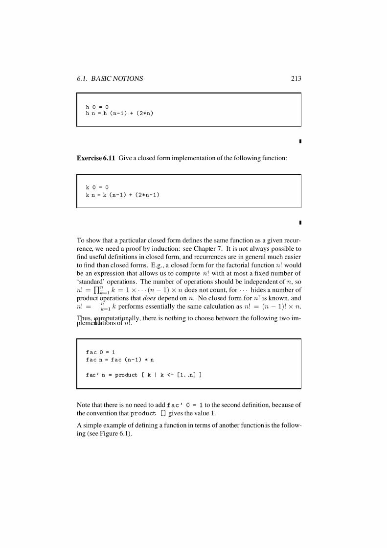
7/16/2019 The Haskell Road to Logic Maths and Programming
http://slidepdf.com/reader/full/the-haskell-road-to-logic-maths-and-programming-5634fa29ef7e9 224/448
6.1. BASIC NOTIONS 213
h 0 = 0h n = h (n-1) + (2*n)
Exercise 6.11 Give a closed form implementation of the following function:
k 0 = 0
k n = k (n-1) + (2*n-1)
To show that a particular closed form defines the same function as a given recur-
rence, we need a proof by induction: see Chapter 7. It is not always possible to
find useful definitions in closed form, and recurrences are in general much easier
to find than closed forms. E.g., a closed form for the factorial function n! would
be an expression that allows us to compute n! with at most a fixed number of
‘standard’ operations. The number of operations should be independent of n, so
n! =nk=1 k = 1 × · · · (n − 1) × n does not count, for · · · hides a number of
product operations that does depend on n. No closed form for n! is known, and
n! = nk=1 k performs essentially the same calculation as n! = (n − 1)! × n.
Thus, computationally, there is nothing to choose between the following two im-plementations of n!.
fac 0 = 1
fac n = fac (n-1) * n
fac’ n = product [ k | k <- [1..n] ]
Note that there is no need to add fac’ 0 = 1 to the second definition, because of
the convention that product [] gives the value 1.
A simple example of defining a function in terms of another function is the follow-
ing (see Figure 6.1).

7/16/2019 The Haskell Road to Logic Maths and Programming
http://slidepdf.com/reader/full/the-haskell-road-to-logic-maths-and-programming-5634fa29ef7e9 225/448
214 CHAPTER 6. FUNCTIONS
-2 -1 0 1 2
0
1
2
3
4
0 1 2
0
1
2
3
4
Figure 6.1: Restricting the function λx.x2.
Definition 6.12 (Restrictions) Suppose that f : X −→ Y and A ⊆ X . The
restriction of f to A is the function h : A → Y defined by h(a) = f (a). The
notation for this function is f A.
Here is the implementation, for functions implemented as type a - > b:
restrict :: Eq a => (a -> b) -> [a] -> a -> b
restrict f xs x | elem x xs = f x
| otherwise = error "argument not in domain"
And this is the implementation for functions implemented as lists of pairs:
restrictPairs :: Eq a => [(a,b)] -> [a] -> [(a,b)]
restrictPairs xys xs = [ (x,y) | (x,y) <- xys, elem x xs ]
Definition 6.13 (Image, Co-image) Suppose that f : X −→ Y , A ⊆ X and
B⊆
Y .
1. f [A] = f (x) | x ∈ A is called the image of A under f ;

7/16/2019 The Haskell Road to Logic Maths and Programming
http://slidepdf.com/reader/full/the-haskell-road-to-logic-maths-and-programming-5634fa29ef7e9 226/448
6.1. BASIC NOTIONS 215
2. f −1[B] =
x
∈X
|f (x)
∈B
is called the co-image of B under f .
From this definition we get:
1. f [X ] = ran(f ),
2. f −1[Y ] = dom (f ),
3. y ∈ f [A] ⇔ ∃x ∈ A(y = f (x)),
4. x ∈ f −1[B] ⇔ f (x) ∈ B.
From 3. it follows that x ∈ A ⇒ f (x) ∈ f [A]. But note that we do not
necessarily have that f (x) ∈ f [A] ⇒ x ∈ A. (Example: f = (0, 2), (1, 2),
x = 0, A = 1.)
Two Types of Brackets. Distinguish f (a) and f [A]. The notation f (a) pre-
supposes that a ∈ dom (f ). Then, f (a) is the f -value of a. The notation f [A]presupposes A ⊆ dom (f ). Then f [A] is the set of values f (x) where x ∈ A.
Remark. Many texts do not employ f [ ] but use f ( ) throughout. In that case,
you have to figure out from the context what is meant.
In the expression f −1[B], the part f −1 has no meaning when taken by itself. The
notation f −1 will be used later on for the inverse function corresponding to f .Such an inverse only exists if f happens to be a bijection. However, the notation
f −1[B] is always meaningful and does not presuppose bijectivity.
Here are the implementations of image and co-image:
image :: Eq b => (a -> b) -> [a] -> [b]
image f xs = nub [ f x | x <- xs ]
coImage :: Eq b => (a -> b) -> [a] -> [b] -> [a]
coImage f xs ys = [ x | x <- xs, elem (f x) ys ]
This gives:
FCT> image (*2) [1,2,3]
[2,4,6]FCT> coImage (*2) [1,2,3] [2,3,4]
[1,2]

7/16/2019 The Haskell Road to Logic Maths and Programming
http://slidepdf.com/reader/full/the-haskell-road-to-logic-maths-and-programming-5634fa29ef7e9 227/448
216 CHAPTER 6. FUNCTIONS
And here are the versions for functions represented as lists of pairs:
imagePairs :: (Eq a, Eq b) => [(a,b)] -> [a] -> [b]
imagePairs f xs = image (list2fct f) xs
coImagePairs :: (Eq a, Eq b) => [(a,b)] -> [a] -> [b] -> [a]
coImagePairs f xs ys = coImage (list2fct f) xs ys
Exercise 6.14 Consider the relation R = (0, 4), (1, 2), (1, 3).
1. Is R a function?
If so, determine dom (R) and ran(R).
2. Remember: R−1 = (b, a) | (a, b) ∈ R is the inverse of the relation R.
(Definition 5.7, p. 163).
Is R−1 a function?
If so, determine dom (R−1) and ran(R−1).
Exercise 6.15 Suppose that f : X −→ Y and A ⊆ X . Verify:
1. f [A] = ran(f A),
2. f [dom (f )] = ran(f ),
3. f −1[B] = dom (f ∩ (X × B)),
4. f −1[ran(f )] = dom (f ),
5. f A = f ∩ (A × Y ).
Exercise 6.16 Let X =
0, 1, 2, 3
, Y =
2, 3, 4, 5
, f =
(0, 3), (1, 2), (2, 4), (3, 2)
.
Determine f 0, 3, f [1, 2, 3] and f −1[2, 4, 5]. Next, check your answers
with the implementation.
7/16/2019 The Haskell Road to Logic Maths and Programming
http://slidepdf.com/reader/full/the-haskell-road-to-logic-maths-and-programming-5634fa29ef7e9 228/448
6.1. BASIC NOTIONS 217
Exercise 6.17 Suppose that f : A
→Y , g : B
→Y , and A
∩B =
∅. Show that
f ∪ g : A ∪ B → Y.
What if A ∩ B = ∅?
Exercise 6.18* Let A be a partition of X . For every component A ∈ A a function
f A : A → Y is given. Show, thatA∈A f A : X → Y .
Example 6.19 Suppose that f : X → Y and A, B ⊆ X . We show that f [A −B] ⊇ f [A] − f [B].
Assume that y
∈f [A]
−f [B]. Then y
∈f [A] and y
∈f [B]. From the first we
obtain x ∈ A such that y = f (x). From the second we see that x ∈ B (otherwise,y = f (x) ∈ f [B]). So, x ∈ A − B, and y = f (x) ∈ f [A − B].
To see that the inclusion cannot be replaced by an equality, take X = Y = A =0, 1, B = 1, and let f be given by f (x) = 0. Then f [A−B] = f [0] = 0and f [A] − f [B] = 0 − 0 = ∅.
Next, suppose that f : X → Y and C, D ⊆ Y . We show that f −1[C − D] =f −1[C ] − f −1[D]:
x ∈ f −1[C − D] ⇐⇒ f (x) ∈ C − D
⇐⇒ (f (x) ∈ C ) ∧ (f (x) ∈ D)
⇐⇒ x ∈ f −1[C ] ∧ x ∈ f −1[D]
⇐⇒ x ∈ f −1
[C ] − f −1
[D].
The required equality follows using Extensionality.
Exercise 6.20 Suppose that f : X → Y , A, B ⊆ X , and C, D ⊆ Y . See example
6.19. Show:
1. A ⊆ B ⇒ f [A] ⊆ f [B];
C ⊆ D ⇒ f −1[C ] ⊆ f −1[D],
2. f [A ∪ B] = f [A] ∪ f [B];
f [A ∩ B] ⊆ f [A] ∩ f [B],
3. f −1[C ∪ D] = f −1[C ] ∪ f −1[D];
f −1[C ∩ D] = f −1[C ] ∩ f −1[D],

7/16/2019 The Haskell Road to Logic Maths and Programming
http://slidepdf.com/reader/full/the-haskell-road-to-logic-maths-and-programming-5634fa29ef7e9 229/448
218 CHAPTER 6. FUNCTIONS
4. f [f −1[C ]]
⊆C ;
f −1[f [A]] ⊇ A.
Give simple examples to show that the inclusions in 2 and 4 cannot be replaced by
equalities.
6.2 Surjections, Injections, Bijections
If X is the domain of a function f , then for each x ∈ X there is only one ywith (x, y) ∈ f . However, there may be other elements z ∈ X with (z, y) ∈ f .Functions for which this does not happen warrant a special name.
If f is a function from X to Y , then there may be elements of Y that are not inf [X ]. Again, functions for which this does not happen warrant a special name.
Definition 6.21 (Surjections, Injections, Bijections)
A function f : X −→ Y is called
1. surjective, or a surjection, or onto Y , if every element b ∈ Y occurs as a
function value of at least one a ∈ X , i.e., if f [X ] = Y ;
2. injective, an injection, or one-to-one, if every b ∈ Y is value of at most one
a ∈ X ;
3. bijective or a bijection if it is both injective and surjective.
Example 6.22 Most functions are neither surjective, nor injective. For instance,
• sin : R → R is not surjective (e.g., 2 ∈ R is not a value) and not injective
(sin0 = sin π).
• The identity function 1X : X → X is a bijection, whatever the set X .
• Let A be a set. According to Theorems 5.87and 5.94, the function that trans-
forms an equivalence R on A into its quotient A/R is a bijection between
the set of equivalences and the set of partitions on A.
•Consider f =
(0, 1), (1, 0), (2, 1)
. Thus, dom (f ) =
0, 1, 2
. The func-
tion
f : 0, 1, 2−→0, 1

7/16/2019 The Haskell Road to Logic Maths and Programming
http://slidepdf.com/reader/full/the-haskell-road-to-logic-maths-and-programming-5634fa29ef7e9 230/448
6.2. SURJECTIONS, INJECTIONS, BIJECTIONS 219
is surjective, but
f : 0, 1, 2−→0, 1, 2is not surjective. The concept of surjectivity presupposes that of a co-
domain. Cf. 6.5 (p. 210). However, whatever this co-domain, f clearly
is not injective, since 0 and 2 have the same image.
If the domain of a function is represented as a list, the injectivity test can be im-
plemented as follows:
injective :: Eq b => (a -> b) -> [a] -> Bool
injective f [] = Trueinjective f (x:xs) =
notElem (f x) (image f xs) && injective f xs
Similarly, if the domain and co-domain of a function are represented as lists, the
surjectivity test can be implemented as follows:
surjective :: Eq b => (a -> b) -> [a] -> [b] -> Bool
surjective f xs [] = True
surjective f xs (y:ys) =
elem y (image f xs) && surjective f xs ys
Exercise 6.23 Implement a test for bijectivity.
Exercise 6.24 Implement tests
injectivePairs, surjectivePairs, bijectivePairs
for functions represented as lists of pairs.
Proving that a Function is Injective/Surjective. The following implication is a
useful way of expressing that f is injective:
f (x) = f (y) =⇒ x = y.
The proof schema becomes:

7/16/2019 The Haskell Road to Logic Maths and Programming
http://slidepdf.com/reader/full/the-haskell-road-to-logic-maths-and-programming-5634fa29ef7e9 231/448
220 CHAPTER 6. FUNCTIONS
To be proved: f is injective.
Proof:
Let x, y be arbitrary, and suppose f (x) = f (y)....
Thus x = y.
The contraposition of f (x) = f (y) =⇒ x = y, i.e.,
x = y =⇒ f (x) = f (y),
of course says the same thing differently, so an equivalent proof schema is:
To be proved: f is injective.
Proof:
Let x, y be arbitrary, and suppose x = y.
...
Thus f (x) = f (y).
That f : X → Y is surjective is expressed by:
∀b ∈ Y ∃a ∈ X f (a) = b.
This gives the following pattern for a proof of surjectivity:
To be proved: f : X → Y is surjective.
Proof:
Let b be an arbitrary element of Y ....
Thus there is an a ∈ X with f (a) = b.
Exercise 6.25 Are the following functions injective? surjective?
7/16/2019 The Haskell Road to Logic Maths and Programming
http://slidepdf.com/reader/full/the-haskell-road-to-logic-maths-and-programming-5634fa29ef7e9 232/448
6.2. SURJECTIONS, INJECTIONS, BIJECTIONS 221
1. sin : R+
→R (N.B.: R+ =
x
∈R
|0 < x
),
2. sin : R → [−1, +1],
3. sin : [−1, +1] → [−1, +1],
4. ex : R → R,
5. tan : R → R,
6. log : R+ → R,
7.√
: R+ → R+.
Remark. The functions of Exercise 6.25 are all predefined in Haskell: sin, exp,
tan, log, sqrt. The base of the natural logarithm, Napier’s number e, is given by
exp 1.
Exercise 6.26 Give a formula for the number of injections from an n-element set
A to a k-element set B.
Exercise 6.27 Implement a function
injs :: [Int] -> [Int] -> [[(Int,Int)]]
that takes a finite domain and a finite codomain of type Int and produces the list
of all injections from domain to codomain, given as lists of integer pairs.
Exercise 6.28 The bijections on a finite set A correspond exactly to the permuta-tions of A. Implement a function
perms :: [a] -> [[a]]
that gives all permutations of a finite list. The call perms [1,2,3] should yield:
[[1,2,3],[2,1,3],[2,3,1],[1,3,2],[3,1,2],[3,2,1]]
Hint: to get the permutations of (x:xs), take all the possible ways of inserting x
in a permutation of xs.

7/16/2019 The Haskell Road to Logic Maths and Programming
http://slidepdf.com/reader/full/the-haskell-road-to-logic-maths-and-programming-5634fa29ef7e9 233/448
222 CHAPTER 6. FUNCTIONS
6.3 Function Composition
Definition 6.29 (Composition) Suppose that f : X −→ Y and g : Y −→ Z .Thus, the co-domain of f coincides with the domain of g. The composition of f and g is the function g f : X −→ Z defined by
(g f )(x) = g(f (x)).
(“First, apply f , next, apply g” — thanks to the usual “prefix”-notation for func-
tions, the f and the g are unfortunately in the reverse order in the notation g f .To keep this reverse order in mind it is good practice to refer to g f as “g after
f ”.)
N.B.: The notation g
f presupposes that the co-domain of f and the domain of
g are the same. Furthermore, g f has the domain of f and the co-domain of g.
Function composition is predefined in Haskell, as follows:
(.) :: (b -> c) -> (a -> b) -> (a -> c)
(f . g) x = f (g x)
Example 6.30 Haskell has a general procedure negate for negating a number.The effect of first taking the absolute value, then negating can now be got by
means of (negate . abs):
Prelude> (negate . abs) 5
-5
Prelude> (negate . abs) (-7)
-7
Prelude>
Example 6.31 Another example from Prelude.hs is:
even n = n ‘rem‘ 2 == 0odd = not . even
7/16/2019 The Haskell Road to Logic Maths and Programming
http://slidepdf.com/reader/full/the-haskell-road-to-logic-maths-and-programming-5634fa29ef7e9 234/448
6.3. FUNCTION COMPOSITION 223
Exercise 6.32 Implement an operation comp for composition of functions repre-
sented as lists of pairs.
Example 6.33 In analysis, compositions abound. E.g., if f : R → R+ is x →x2 + 1, and g : R+ → R is x → √
x, then g f : R → R is x → √ x2 + 1:
(g f )(x) = g(f (x)) = g(x2 + 1) =√
x2 + 1.
The identity function behaves as a unit element for composition (see Example 6.1
for 1X):
Fact 6.34 If f : X → Y , then f 1X = 1Y f = f .
Suppose that f : X → Y , g : Y → Z and h : Z → U . There are now two ways
to define a function from X to U : (i) (h g) f , and (ii) = h (g f ). The next
lemma says that these functions coincide. Thus, composition is associative; and
we can safely write h g f if we mean either of these.
Lemma 6.35 If f : X → Y , g : Y → Z and h : Z → U , then (h g) f =h (g f ).
Proof. Suppose that x ∈ X . Then:
((hg)f )(x) = (hg)(f (x)) = h(g(f (x))) = h((gf )(x)) = (h(gf ))(x).
The functions (h g) f and h (g f ) have the same domain (X ) and co-domain
(U ) and, on this domain, show the same action. Thus, they are (6.5, p. 210) equal.
Lemma 6.36 Suppose that f : X −→ Y , g : Y −→ Z . Then:
1. g f injective =⇒ f injective,
2. g f surjective =⇒ g surjective,
3. f and g injective =⇒ g f injective,
4. f and g surjective =⇒ g f surjective.
Proof. We prove 1, 2 and 4.
1. Given: g f injective, i.e., (g f )(a1) = (g f )(a2) ⇒ a1 = a2.
To be proved: f injective, i.e., f (a1) = f (a2) ⇒ a1 = a2.

7/16/2019 The Haskell Road to Logic Maths and Programming
http://slidepdf.com/reader/full/the-haskell-road-to-logic-maths-and-programming-5634fa29ef7e9 235/448
224 CHAPTER 6. FUNCTIONS
Proof: Assume f (a1) = f (a2). Then of course, g(f (a1)) = g(f (a2)). (Applying
g twice to the same argument must produce the same value twice.) But then,(g f )(a1) = g(f (a1)) = g(f (a2)) = (g f )(a2). The given now shows that
a1 = a2.
2. Given: g f surjective.
To be proved: g surjective. I.e., ∀c ∈ Z ∃b ∈ Y (g(b) = c).
Proof: Assume c ∈ Z . Wanted: b ∈ Y such that g(b) = c. Since gf is surjective,
there is a ∈ X such that (g f )(a) = c. But, g(f (a)) = (g f )(a). I.e., b = f (a)is the element looked for.
4. Given: f and g surjective.
To be proved: g f surjective. I.e., every c ∈ Z is a value of g f .Proof: Assume c ∈ Z . Since g is surjective, b ∈ Y exists such that g(b) = c.
Since f is surjective, a
∈X exists such that f (a) = b. It follows that (g
f )(a) =
g(f (a)) = g(b) = c. So, a is the element looked for.
Note that there are statements in the spirit of Lemma 6.36 that do not hold. In
particular, from the fact that g f is injective, it does not follow that g is injective.
Consider the case where f is the (empty) function from ∅ to Y , and g an arbitrary
non-injective function from Y → Z . Then g f is the (empty) function from ∅ to
Z , which is surely injective. But g by assumption is not injective.
For an example in which g f is bijective, but g not injective and f not surjective,
take f : N → N given by f (n) = n + 1 and g : N → N given by
g(n) =
n if n = 0n
−1 if n 1.
Clearly, gf is the identity onN, but f is not a surjection, and g is not an injection.
Exercise 6.37 Can you think up an example with gf bijective, but g not injective
and f not surjective, with the domain of f finite? If yes, give the example, if no,
prove that this is impossible.
Exercise 6.38 The function f : 0, 1, 2, 3, 4 → 0, 1, 2, 3, 4 is defined by the
following table:
x 0 1 2 3 4
f (x) 1 2 0 0 3
(f f )(x)
(f f f )(x)(f f f f )(x)

7/16/2019 The Haskell Road to Logic Maths and Programming
http://slidepdf.com/reader/full/the-haskell-road-to-logic-maths-and-programming-5634fa29ef7e9 236/448
6.3. FUNCTION COMPOSITION 225
1. Determine the compositions f
f , f
f
f and f
f
f
f by completing
the table.
2. How many elements has the set f, f f, f f f , . . .? (N.B.: the elements
are functions!)
3. Exhibit a function g : 0, 1, 2, 3, 4 → 0, 1, 2, 3, 4 such that g, g g, g g g , . . . has 6 elements.
Exercise 6.39* Suppose that A is a finite set and f : A → A is a bijection. Then
f 1 = f , f 2 = f
f , f 3 = f
f
f ,. . . all are bijections : A→
A.
1. Show that, somewhere in this sequence, there occurs the bijection 1A. I.e.,
a number n exists such that f n = 1A.
2. Suppose that A has k elements. Can you give an upper bound for n?
Exercise 6.40 Suppose that h : X → X satisfies h h h = 1X . Show that h is
a bijection.
Exhibit a simple example of a set X and a function h : X
→X such that h
h
h =
1X , whereas h = 1X .
Exercise 6.41 Prove Lemma 6.36.3.
Exercise 6.42 Suppose that f : X → Y and g : Y → Z are such that g f is
bijective. Show that f is surjective iff g is injective.
Exercise 6.43 Suppose that limi→∞ ai = a, and that f : N → N is injective.Show that limi→∞ af (i) = a. (Cf. also Exercise 8.22, p. 318.)

7/16/2019 The Haskell Road to Logic Maths and Programming
http://slidepdf.com/reader/full/the-haskell-road-to-logic-maths-and-programming-5634fa29ef7e9 237/448
226 CHAPTER 6. FUNCTIONS
6.4 Inverse Function
If we consider f : X → Y as a relation, then we can consider its relational
inverse: the set of all (y, x) with (x, y) ∈ f . However, there is no guarantee that
the relational inverse of a function is again a function. In case f is injective, we
know that the relational inverse of f is a partial function (some elements in the
domain may not have an image). If f is also surjective, we know that the relational
inverse of f is a function. Thus, an inverse function of f has to satisfy some special
requirements.
Figure 6.2: Inverse of the function λx.x2 (restricted to R+).
Definition 6.44 (Inverse Function) Suppose that f : X → Y . A function g :Y → X is an inverse of f if both (i) g f = 1X , and (ii) f g = 1Y .
The next theorem says all there is to know about inverses. Its proof describes how
to find an inverse if there is one.
Note that, by the first part of the theorem, we can safely talk about the inverse of afunction (provided there is one).
Theorem 6.45
1. A function has at most one inverse.
2. A function has an inverse iff it is bijective.
Proof. (1) Suppose that g and h are both inverses of f : X → Y . Then g =1X g = (h f ) g = h (f g) = h 1Y = h.
(2) (Only if.) Assume that g is inverse of f . Then since g
f = 1X
is injective, by
Lemma 6.36.1 f also is injective. And since f g = 1Y is surjective, by 6.36.2 f also is surjective.

7/16/2019 The Haskell Road to Logic Maths and Programming
http://slidepdf.com/reader/full/the-haskell-road-to-logic-maths-and-programming-5634fa29ef7e9 238/448
6.4. INVERSE FUNCTION 227
(If.) Suppose that f is a bijection. I.e., for every y
∈Y there is exactly one x
∈X
such that f (x) = y. Thus, we can define a function g : Y → X by letting g(y) bethe unique x such that f (x) = y.
Then g is inverse of f : firstly, if x ∈ X , then g(f (x)) = x; secondly, if y ∈ Y ,then f (g(y)) = y.
Notation. If f : X → Y is a bijection, then its unique inverse is denoted by f −1.
Remark. If f : X → Y is a bijection, then f −1 can denote either the inverse
function : Y → X , or the inverse of f considered as a relation. But from the proof
of Theorem 6.45 it is clear that these are the same.
Example 6.46 The real function f that is given by f (x) = 9
5
x + 32 allows us
to convert degrees Celcius into degrees Fahrenheit. The inverse function f −1 is
given by f −1(x) = 59 (x − 32); it converts degrees Fahrenheit back into degrees
Celsius. Here are integer approximations:
c2f, f2c :: Int -> Int
c2f x = div (9 * x) 5 + 32
f2c x = div (5 * (x - 32)) 9
*Left and Right-inverse. Note that there are two requirements on inverse func-
tions. If f : X → Y , g : Y → X , and we have that g f = 1X only, then g is
called left-inverse of f and f right-inverse of g.
Example 6.47 The class Enum is (pre-)defined in Haskell as follows:
class Enum a where
succ, pred :: a -> a
toEnum :: Int -> a
fromEnum :: a -> Int
fromEnum should be a left-inverse of toEnum:
7/16/2019 The Haskell Road to Logic Maths and Programming
http://slidepdf.com/reader/full/the-haskell-road-to-logic-maths-and-programming-5634fa29ef7e9 239/448
228 CHAPTER 6. FUNCTIONS
fromEnum (toEnum x) = x
This requirement cannot be expressed in Haskell, so it is the responsibility of the
programmer to make sure that it is satisfied. Examples of use of toEnum and
fromEnum from Prelude.hs:
ord :: Char -> Int
ord = fromEnum
chr :: Int -> Char
chr = toEnum
Exercise 6.48 Show: if f : X → Y has left-inverse g and right-inverse h, then f is a bijection and g = h = f −1.
Exercise 6.49 Suppose that f : X → Y and g : Y → X . Show that the following
are equivalent.
1. g f = 1X ,
2. (f (x), x) | x ∈ X ⊆ g.
Exercise 6.50 X = 0, 1, Y = 2, 3, 4, 5, f = (0, 3), (1, 4). We have that
f : X → Y . How many functions g : Y → X have the property, that g f = 1X?
Exercise 6.51 Give an example of an injection f : X → Y for which there is no
g : Y → X such that g f = 1X .
Exercise 6.52* Show that if f : X
→Y is surjective, a function g : Y
→X exists
such that f g = 1Y .
7/16/2019 The Haskell Road to Logic Maths and Programming
http://slidepdf.com/reader/full/the-haskell-road-to-logic-maths-and-programming-5634fa29ef7e9 240/448
6.5. PARTIAL FUNCTIONS 229
Exercise 6.53 How many right-inverses are there to the function
(0, 5), (1, 5), (2, 5), (3, 6), (4, 6)
(domain: 0, 1, 2, 3, 4, co-domain: 5, 6)?
Exercise 6.54 1. The surjection f : R → R+ is defined by f (x) = x2. Give
three different right-inverses for f .
2. Same question for g : [0, π] → [0, 1] defined by g(x) = sin x.
Exercise 6.55 Suppose that f : X → Y is a surjection and h : Y → X . Showthat the following are equivalent.
1. h is right-inverse of f ,
2. h ⊆ (f (x), x) | x ∈ X .
Exercise 6.56* Show:
1. Every function that has a surjective right-inverse is a bijection.
2. Every function that has an injective left-inverse is a bijection.
6.5 Partial Functions
A partial function from X to Y is a function with its domain included in X and
its range included in Y . If f is a partial function from X to Y we write this as f :X → Y . It is immediate from this definition that f : X → Y iff dom (f ) ⊆ X and f dom (f ) : dom (f ) → Y .
A way of defining a partial function (using ⊥ for ‘undefined’):
f (x) =
⊥ if ...t otherwise

7/16/2019 The Haskell Road to Logic Maths and Programming
http://slidepdf.com/reader/full/the-haskell-road-to-logic-maths-and-programming-5634fa29ef7e9 241/448
230 CHAPTER 6. FUNCTIONS
The computational importance of partial functions is in the systematic perspective
they provide on exception handling. In Haskell, the crude way to deal with excep-tions is by a call to the error abortion function error. The code below implements
partial functions succ0 and succ1. succ0 is partial because the pattern (x+1)
only matches positive integers. succ1 has an explicit call to error. The disad-
vantage of these implementations is that they are called by another program, the
execution of that other program may abort.
succ0 :: Integer -> Integer
succ0 (x+1) = x + 2
succ1 :: Integer -> Integer
succ1 = \ x -> if x < 0
then error "argument out of range"
else x+1
This uses the reserved keywords if, then and else, with the obvious meanings.
A useful technique for implementing partial functions is to represent a partial func-
tion from type a to type b as a function of type a -> [b]. In case of an exception,
the empty list is returned. If a regular value is computed, the unit list with the
computed value is returned.
succ2 :: Integer -> [Integer]
succ2 = \ x -> if x < 0 then [] else [x+1]
Composition of partial functions implemented with unit lists can be defined as
follows:
pcomp :: (b -> [c]) -> (a -> [b]) -> a -> [c]
pcomp g f = \ x -> concat [ g y | y <- f x ]
As an alternative to this trick with unit lists Haskell has a special data type for im-
plementing partial functions, the data type Maybe, which is predefined as follows.
7/16/2019 The Haskell Road to Logic Maths and Programming
http://slidepdf.com/reader/full/the-haskell-road-to-logic-maths-and-programming-5634fa29ef7e9 242/448
6.5. PARTIAL FUNCTIONS 231
data Maybe a = Nothing | Just a
deriving (Eq, Ord, Read, Show)
maybe :: b -> (a -> b) -> Maybe a -> b
maybe n f Nothing = n
maybe n f (Just x) = f x
Here is a third implementation of the partial successor function:
succ3 :: Integer -> Maybe Integer
succ3 = \ x -> if x < 0 then Nothing else Just (x+1)
The use of the predefined function maybe is demonstrated in the definition of com-
position for functions of type a -> Maybe b.
mcomp :: (b -> Maybe c) -> (a -> Maybe b) -> a -> Maybe c
mcomp g f = (maybe Nothing g) . f
Of course, the maybe function allows for all kinds of ways to deal with excep-
tions. E.g., a function of type a -> Maybe b can be turned into a function of type
a - > b by the following part2error conversion.
part2error :: (a -> Maybe b) -> a -> b
part2error f = (maybe (error "value undefined") id) . f
Exercise 6.57 Define a partial function
stringCompare :: String -> String -> Maybe Ordering

7/16/2019 The Haskell Road to Logic Maths and Programming
http://slidepdf.com/reader/full/the-haskell-road-to-logic-maths-and-programming-5634fa29ef7e9 243/448
232 CHAPTER 6. FUNCTIONS
for ordering strings consisting of alphabetic characters in the usual list order. If a
non-alphabetic symbol occurs, the ordering function should return Nothing. UseisAlpha for the property of being an alphabetic character.
6.6 Functions as Partitions
In practice, equivalences are often defined by way of functions. Par abus de lan-
guage functions sometimes are called partitions for that reason. Examples of such
functions on the class of all people: “the gender of x” (partitions in males and fe-
males), “the color of x” (partitions in races), “the age of x” (some hundred equiv-
alence classes). The next exercise explains how this works and asks to show that
every equivalence is obtained in this way.
Exercise 6.58 Suppose that f : A → I is a surjection. Define the relation R on Aby: aRb :≡ f (a) = f (b). Thus, R = (a, b) ∈ A2 | f (a) = f (b). Show:
1. R is an equivalence on A,
2. A/R = f −1[i] | i ∈ I ,
3. for every equivalence S on A there is a function g on A such that aSb ⇔g(a) = g(b).
Example 6.59 For any n ∈ Z with n = 0, let the function RMn :: Z → Z
be given by RMn(m) := r where 0 r < n and there is some a ∈ Z with
m = an + r. Then RMn induces the equivalence ≡n on Z.
Here is a Haskell implementation of a procedure that maps a function to the equiv-
alence relation inducing the partition that corresponds with the function:
fct2equiv :: Eq a => (b -> a) -> b -> b -> Bool
fct2equiv f x y = (f x) == (f y)
You can use this to test equality modulo n, as follows:

7/16/2019 The Haskell Road to Logic Maths and Programming
http://slidepdf.com/reader/full/the-haskell-road-to-logic-maths-and-programming-5634fa29ef7e9 244/448
6.6. FUNCTIONS AS PARTITIONS 233
FCT> fct2equiv (‘rem‘ 3) 2 14
True
Exercise 6.60* Suppose that f : A → B.
1. Show: If f is an injection, then for all sets C and for every g : A → C there
is a function h : B → C such that g = h f .
2. Show: For all sets C , if to every g : A → C there is a function h : B → C such that g = h f , then f is an injection.
Exercise 6.61* Suppose that R is an equivalence on the set A. Show: for every
equivalence S ⊇ R on A there exists a function g : A/R → A/S such that, fora ∈ A: | a |S = g(| a |R).
Exercise 6.62* Suppose that ∼ is an equivalence on A, and that f : A2 → A is a
binary function such that for all a,b,x,y ∈ A:
a ∼ x ∧ b ∼ y =⇒ f (a, b) ∼ f (x, y).
Show that a unique function f ∼ : (A/∼)2 → B exists such that, for a, b ∈ A:
f ∼(|a|, |b|) = |f (a, b)|.
Exercise 6.63* Suppose that∼
is an equivalence on A, and that R⊆
A2 is a
relation such that for all a,b,x,y ∈ A:
a ∼ x ∧ b ∼ y ∧ aRb ⇒ xRy.
Show that a unique relation R∼ ⊆ (A/ ∼)2 exists such that for all a, b ∈ A:
|a|R∼|b| ⇔ aRb.
Exercise 6.64* A and B are sets, with B = ∅. Define ∼ on A × B by: (a, b) ∼(x, y) ≡ a = x.
1. Show that ∼ is an equivalence on A × B.
2. Exhibit a bijection : (A×B)/∼ −→ A from the quotient of A×B modulo
∼ to A.

7/16/2019 The Haskell Road to Logic Maths and Programming
http://slidepdf.com/reader/full/the-haskell-road-to-logic-maths-and-programming-5634fa29ef7e9 245/448
234 CHAPTER 6. FUNCTIONS
3. Exhibit, for every equivalence class, a bijection between the class and B.
Equivalence classes (restricted to a list) for an equivalence defined by a function
are generated by the following Haskell function:
block :: Eq b => (a -> b) -> a -> [a] -> [a]
block f x list = [ y | y <- list, f x == f y ]
This gives:
FCT> block (‘rem‘ 3) 2 [1..20]
[2,5,8,11,14,17,20]
FCT> block (‘rem‘ 7) 4 [1..20]
[4,11,18]
Exercise 6.65 Functions can be used to generate equivalences, or equivalently,partitions. In an implementation we use list partitions; see Exercise 5.109 for adefinition. Implement an operation fct2listpart that takes a function and adomain and produces the list partition that the function generates on the domain.Some example uses of the operation are:
Main> fct2listpart even [1..20]
[[1,3,5,7,9,11,13,15,17,19],[2,4,6,8,10,12,14,16,18,20]]
Main> fct2listpart (\ n -> rem n 3) [1..20][[1,4,7,10,13,16,19],[2,5,8,11,14,17,20],[3,6,9,12,15,18]]
Exercise 6.66 Give an formula for the number of surjections from an n-element
set A to a k-element set B. (Hint: each surjection f : A → B induces a partition.
These partitions can be counted with the technique from Example 5.103.)
6.7 Products
Definition 6.67 (Product) Suppose that, for every element i∈
I a non-empty set
X i is given. The product i∈I X i is the set of all functions f for which dom (f ) =
I and such that for all i ∈ I : f (i) ∈ X i.

7/16/2019 The Haskell Road to Logic Maths and Programming
http://slidepdf.com/reader/full/the-haskell-road-to-logic-maths-and-programming-5634fa29ef7e9 246/448
6.7. PRODUCTS 235
When I =
0, . . . , n
−1
, this product is also written as X 0
× · · · ×X n
−1.
If all X i (i ∈ I ) are the same, X i = X , the product is written as X I . Thus, X I is
the set of all functions f : I → X .
Exercise 6.68* There are now two ways to interpret the expression X 0 × X 1: (i)
asi∈0,1 X i, and (ii) as (x, y) | x ∈ X 0 ∧ y ∈ X 1. Can you explain why
there is no harm in this?
In our implementation language, product types have the form (a,b), (a,b,c),
etcetera.
Exercise 6.69* Let A be any set. Exhibit two different bijections between ℘(A)and
0, 1
A.
Exercise 6.70* Suppose that X and Y are sets. On the set of functions Y X =f | f : X → Y , the relation ≈ is defined by: f ≈ g ≡ there are bijections
i : Y → Y and j : X → X such that i f = g j.
1. Show that ≈ is an equivalence.
2. Show: if f, g : X → Y are injective, then f ≈ g.
3. Suppose that Y = 0, 1, 2 and X = 0, 1, 2, 3.
(a) Show that (0, 0), (1, 0), (2, 1) ≈ (0, 1), (1, 3), (2, 3).
(b) How many equivalence classes has
≈? For every class, produce one
representative.
Exercise 6.71* Suppose that X , Y and Z are sets and that h : Y → Z . Define
F : Y X → Z X by F (g) := h g. Show:
1. if h is injective, then F is injective,
2. if h is surjective, then F is surjective.
Exercise 6.72* Suppose that X = ∅, Y , and Z are sets and that h : X → Y .Define F : Z Y → Z X by F (g) := g h. Show:
7/16/2019 The Haskell Road to Logic Maths and Programming
http://slidepdf.com/reader/full/the-haskell-road-to-logic-maths-and-programming-5634fa29ef7e9 247/448
236 CHAPTER 6. FUNCTIONS
1. if h is injective, then F is surjective,
2. if h is surjective, then F is injective.
6.8 Congruences
A function f : X n → X is called an n-ary operation on X . Addition and multi-
plication are binary operations on N (on Z, on Q, on R, on C).
If one wants to define new structures from old, an important method is taking
quotients for equivalences that are compatible with certain operations.
Definition 6.73 (Congruence) If f be an n-ary operation on A, and R an equiv-
alence on A, then R is a congruence for f (or: R is compatible with f ) if for
all
x1, . . . , xn, y1, . . . , yn ∈ A : x1Ry1, . . . , xnRyn
imply that
f (x1, . . . , xn)Rf (y1, . . . , yn).
If R is a congruence for f , then the operation induced by f on A/R is the operation
f R : (A/R)n → A/R given by
f R(|a1|R, . . . , |an|R) := |f (a1, . . . , an)|R.
If (A, f ) is a set with an operation f on it and R is a congruence for f , then
(A/R, f R) is the quotient structure defined by R.
Example 6.74 Consider the modulo n relation on Z. Suppose m ≡n m and
k ≡n k. Then (Proposition 5.65) there are a, b ∈ Z with m = m + an and
k = k + bn. Thus m + k = m + k + (a + b)n, i.e., m + k ≡n m + k. This
shows that ≡n is a congruence for addition. Similarly, it can be shown that ≡n is a
congruence for subtraction. It follows that we can define [m]n + [k]n := [m + k]nand [m]n − [k]n := [m − k]n.
Exercise 6.75 Show that ≡n on Z is a congruence for multiplication, for any n ∈Z with n = 0.

7/16/2019 The Haskell Road to Logic Maths and Programming
http://slidepdf.com/reader/full/the-haskell-road-to-logic-maths-and-programming-5634fa29ef7e9 248/448
6.8. CONGRUENCES 237
Example 6.76 Is
≡n on Z (n
= 0) a congruence for exponentiation, i.e., is it
possible to define exponentiation of classes in Zn by means of:
([k]n)([m]n)
:= [km]n, for k ∈ Z, m ∈ N?
No, for consider the following example: ([2]3)([1]3) = [21]3 = [2]3. Since 1 ≡3 4we also have: ([2]3)([1]3) = ([2]3)([4]3) = [24]3 = [16]3 = [1]3 = [2]3. What
this shows is that the definition is not independent of the class representatives.
Therefore, ≡n is not a congruence for exponentiation.
Example 6.77 The definition of the integers from the natural numbers, in Section
7.2 below, uses the fact that the relation R on N2 given by
(m1, m2)R(n1, n2) :≡ m1 + n2 = m2 + n1
is an equivalence relation, that the relation <R on N2/R given by
|(m1, m2)|R <R |(n1, n2)|R :≡ m1 + n2 < m2 + n1
is properly defined, and moreover, that R is a congruence for addition and multi-
plication on N2.
To check that R is a congruence for addition on N2, where addition on N2 is given
by
(m1, m2) + (n1, n2) := (m1 + n1, m2 + n2),
we have to show that (m1, m2)R( p1, p2) and (n1, n2)R(q 1, q 2) together imply
that (m1, m2) + (n1, n2)R( p1, p2) + (q 1, q 2).
Assume (m1, m2)R( p1, p2) and (n1, n2)R(q 1, q 2). Applying the definition of R,
this gives
m1 + p2 = p1 + m2 and n1 + q 2 = q 1 + n2,
whence
m1 + n1 + p2 + q 2 = n1 + p1 + m2 + n2. (*)
We now have:
(m1, m2) + (n1, n2) = (m1 + n1, m2 + n2),
( p1, p2) + (q 1, q 2) = ( p1 + q 1, p2 + q 2),
and by the definition of R we get from (*) that
(m1, m2) + (n1, n2)R( p1, p2) + (q 1, q 2).
This proves that R is a congruence for addition.

7/16/2019 The Haskell Road to Logic Maths and Programming
http://slidepdf.com/reader/full/the-haskell-road-to-logic-maths-and-programming-5634fa29ef7e9 249/448
238 CHAPTER 6. FUNCTIONS
Exercise 6.78* Show that the relation R on N2 from example 6.77 is a congruence
for the multiplication operation on N2 given by:
(m1, m2) · (n1, n2) := (m1n1 + m2n2, m1n2 + n1m2).
6.9 Further Reading
More on functions in the context of set theory in [DvDdS78]. A logical theory of
functions is developed in the lambda calculus. See [Bar84].
7/16/2019 The Haskell Road to Logic Maths and Programming
http://slidepdf.com/reader/full/the-haskell-road-to-logic-maths-and-programming-5634fa29ef7e9 250/448
Chapter 7
Induction and Recursion
Preview
A very important proof method that is not covered by the recipes from Chapter 3 is
the method of proof by Mathematical Induction. Roughly speaking, mathematical
induction is a method to prove things about objects that can be built from a finite
number of ingredients in a finite number of steps. Such objects can be thought of
as construed by means of recursive definitions. Thus, as we will see in this chapter,
recursive definitions and inductive proofs are two sides of one coin.
module IAR
where
import List
import STAL (display)
7.1 Mathematical Induction
Mathematical induction is a proof method that can be used to establish the truth of
a statement for an infinite sequence of cases 0, 1, 2, . . . . Let P (n) be a property of
239

7/16/2019 The Haskell Road to Logic Maths and Programming
http://slidepdf.com/reader/full/the-haskell-road-to-logic-maths-and-programming-5634fa29ef7e9 251/448
240 CHAPTER 7. INDUCTION AND RECURSION
natural numbers. To prove a goal of the form
∀n
∈N : P (n) one can proceed as
follows:
1. Basis. Prove that 0 has the property P .
2. Induction step. Assume the induction hypothesis that n has property P .Prove on the basis of this that n + 1 has property P .
That’s all. The goal ∀n ∈ N : P (n) follows from this by the principle of mathe-
matical induction.
By the principle of mathematical induction we mean the following fact:
Fact 7.1 For every set X ⊆ N, we have that:
if 0 ∈ X and ∀n ∈ N(n ∈ X ⇒ n + 1 ∈ X ), then X = N.
This fact is obviously true.
The best way to further explain mathematical induction is by way of examples.
Example 7.2 Sum of the Angles of a Convex Polygon.
Suppose we want to prove that the sum of the angles of a convex polygon of n + 3sides is (n + 1)π radians.
d d
d d d
d d d
We can show this by mathematical induction with respect to n, as follows:
Basis For n = 0, the statement runs: the sum of the angles of a convex polygon of
3 sides, i.e., of a triangle, is π radians. We know from elementary geometry
that this is true.
Induction step Assume that the sum of the angles of a convex polygon of n + 3sides is (n + 1)π radians. Take a convex polygon P of n + 4 sides. Then,
since P is convex, we can decompose P into a triangle T and a convex
polygon P of n + 3 sides (just connect edges 1 and 3 of P ). The sum of the
angles of P equals the sum of the angles of T , i.e. π radians, plus the sum
of the angles of P , i.e., by the induction hypothesis, (n + 1)π radians. This
shows that the sum of the angles of P is (n + 2)π radians.
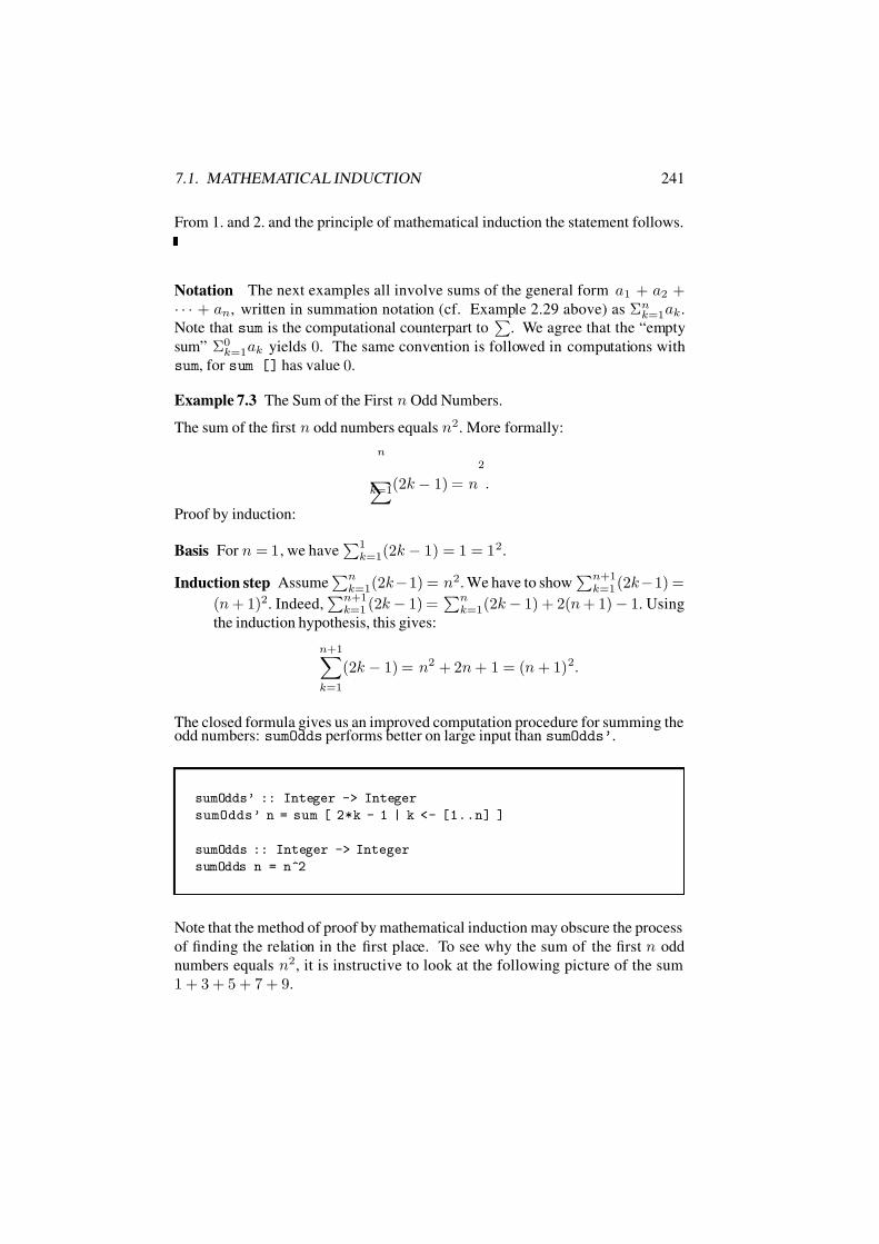
7/16/2019 The Haskell Road to Logic Maths and Programming
http://slidepdf.com/reader/full/the-haskell-road-to-logic-maths-and-programming-5634fa29ef7e9 252/448
7.1. MATHEMATICAL INDUCTION 241
From 1. and 2. and the principle of mathematical induction the statement follows.
Notation The next examples all involve sums of the general form a1 + a2 +· · · + an, written in summation notation (cf. Example 2.29 above) as Σn
k=1ak.
Note that sum is the computational counterpart to
. We agree that the “empty
sum” Σ0k=1ak yields 0. The same convention is followed in computations with
sum, for sum [] has value 0.
Example 7.3 The Sum of the First n Odd Numbers.
The sum of the first n odd numbers equals n2. More formally:
n
k=1(2k − 1) = n
2
.
Proof by induction:
Basis For n = 1, we have1
k=1(2k − 1) = 1 = 12.
Induction step Assumen
k=1(2k−1) = n2. We have to shown+1
k=1 (2k−1) =
(n + 1)2. Indeed,n+1
k=1 (2k − 1) =n
k=1(2k − 1) + 2(n + 1) − 1. Using
the induction hypothesis, this gives:
n+1k=1
(2k − 1) = n2 + 2n + 1 = (n + 1)2.
The closed formula gives us an improved computation procedure for summing theodd numbers: sumOdds performs better on large input than sumOdds’.
sumOdds’ :: Integer -> Integer
sumOdds’ n = sum [ 2*k - 1 | k <- [1..n] ]
sumOdds :: Integer -> Integer
sumOdds n = n^2
Note that the method of proof by mathematical induction may obscure the process
of finding the relation in the first place. To see why the sum of the first n odd
numbers equals n2, it is instructive to look at the following picture of the sum
1 + 3 + 5 + 7 + 9.
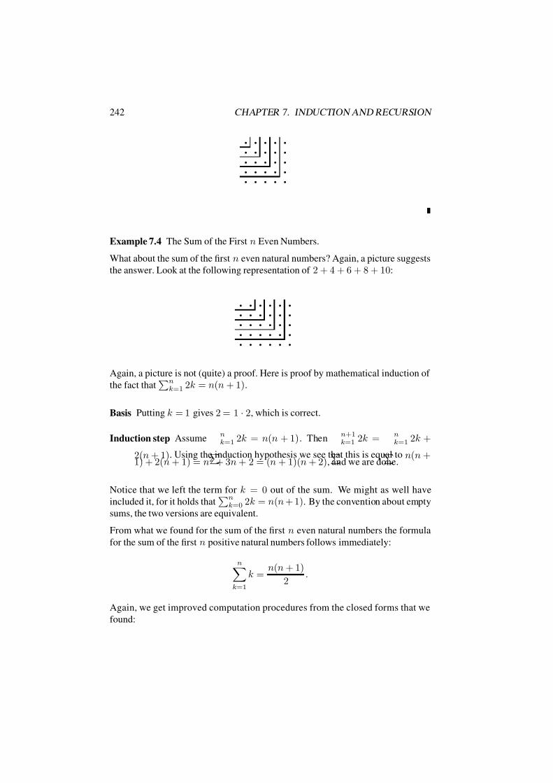
7/16/2019 The Haskell Road to Logic Maths and Programming
http://slidepdf.com/reader/full/the-haskell-road-to-logic-maths-and-programming-5634fa29ef7e9 253/448
242 CHAPTER 7. INDUCTION AND RECURSION
q q q q q
q q q q q
q q q q q
q q q q q
q q q q q
Example 7.4 The Sum of the First n Even Numbers.
What about the sum of the first n even natural numbers? Again, a picture suggests
the answer. Look at the following representation of 2 + 4 + 6 + 8 + 10:
q q q q q q
q q q q q q
q q q q q q
q q q q q q
q q q q q q
Again, a picture is not (quite) a proof. Here is proof by mathematical induction of
the fact thatn
k=1 2k = n(n + 1).
Basis Putting k = 1 gives 2 = 1 · 2, which is correct.
Induction step Assume nk=1 2k = n(n + 1). Then
n+1k=1 2k =
nk=1 2k +
2(n + 1). Using the induction hypothesis we see that this is equal to n(n +1) + 2(n + 1) = n2 + 3n + 2 = (n + 1)(n + 2), and we are done.
Notice that we left the term for k = 0 out of the sum. We might as well have
included it, for it holds thatn
k=0 2k = n(n + 1). By the convention about empty
sums, the two versions are equivalent.
From what we found for the sum of the first n even natural numbers the formula
for the sum of the first n positive natural numbers follows immediately:
nk=1
k =n(n + 1)
2.
Again, we get improved computation procedures from the closed forms that we
found:
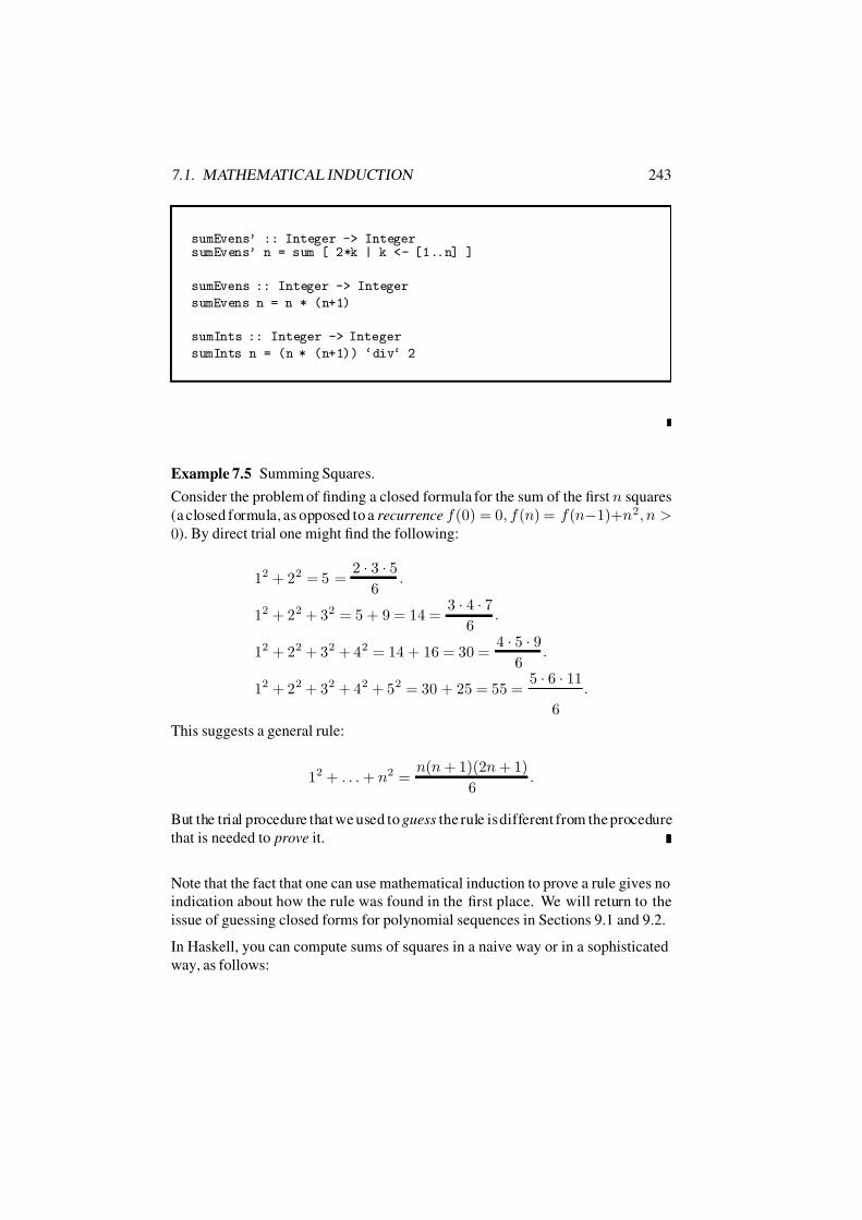
7/16/2019 The Haskell Road to Logic Maths and Programming
http://slidepdf.com/reader/full/the-haskell-road-to-logic-maths-and-programming-5634fa29ef7e9 254/448
7.1. MATHEMATICAL INDUCTION 243
sumEvens’ :: Integer -> IntegersumEvens’ n = sum [ 2*k | k <- [1..n] ]
sumEvens :: Integer -> Integer
sumEvens n = n * (n+1)
sumInts :: Integer -> Integer
sumInts n = (n * (n+1)) ‘div‘ 2
Example 7.5 Summing Squares.
Consider the problem of finding a closed formula for the sum of the first n squares
(a closed formula, as opposed to a recurrence f (0) = 0, f (n) = f (n−1)+n2, n >0). By direct trial one might find the following:
12 + 22 = 5 =2 · 3 · 5
6.
12 + 22 + 32 = 5 + 9 = 14 =3 · 4 · 7
6.
12 + 22 + 32 + 42 = 14 + 16 = 30 =4 · 5 · 9
6.
12 + 22 + 32 + 42 + 52 = 30 + 25 = 55 =5 · 6 · 11
6
.
This suggests a general rule:
12 + . . . + n2 =n(n + 1)(2n + 1)
6.
But the trial procedure that we used to guess the rule is different from the procedure
that is needed to prove it.
Note that the fact that one can use mathematical induction to prove a rule gives no
indication about how the rule was found in the first place. We will return to the
issue of guessing closed forms for polynomial sequences in Sections 9.1 and 9.2.
In Haskell, you can compute sums of squares in a naive way or in a sophisticated
way, as follows:

7/16/2019 The Haskell Road to Logic Maths and Programming
http://slidepdf.com/reader/full/the-haskell-road-to-logic-maths-and-programming-5634fa29ef7e9 255/448
244 CHAPTER 7. INDUCTION AND RECURSION
sumSquares’ :: Integer -> IntegersumSquares’ n = sum [ k^2 | k <- [1..n] ]
sumSquares :: Integer -> Integer
sumSquares n = (n*(n+1)*(2*n+1)) ‘div‘ 6
Again, the insight that the two computation procedures will always give the same
result can be proved by mathematical induction:
Exercise 7.6 Summing Squares. Prove by mathematical induction:
n
k=1
k
2
=
n(n + 1)(2n + 1)
6 .
Example 7.7 Summing Cubes.
Let us move on to the problem of summing cubes. By direct trial one finds:
13 + 23 = 9 = (1 + 2)2.
13 + 23 + 33 = 9 + 27 = 36 = (1 + 2 + 3) 2.
13 + 23 + 33 + 43 = 36 + 64 = 100 = (1 + 2 + 3 + 4)2.
13 + 23 + 33 + 43 + 53 = 100 + 125 = 225 = (1 + 2 + 3 + 4 + 5)2.
This suggests a general rule:
13 + · · · + n3 = (1 + · · · + n)2.
We saw in Example 7.4 that
nk=1
k =n(n + 1)
2,
so the general rule reduces to:
13 + · · · + n3 =
n(n + 1)
2
2
.
So much about finding a rule for the sum of the first n cubes. In Sections 9.1
and 9.2 we will give an algorithm for generating closed forms for polynomial
sequences.

7/16/2019 The Haskell Road to Logic Maths and Programming
http://slidepdf.com/reader/full/the-haskell-road-to-logic-maths-and-programming-5634fa29ef7e9 256/448
7.1. MATHEMATICAL INDUCTION 245
What we found is that sumCubes defines the same function as the naive procedure
sumCubes’ for summing cubes:
sumCubes’ :: Integer -> Integer
sumCubes’ n = sum [ k^3 | k <- [1..n] ]
sumCubes :: Integer -> Integer
sumCubes n = (n*(n+1) ‘div‘ 2)^2
Again, the relation we found suggests a more sophisticated computation proce-
dure, and proving the general relationship between the two procedures is another
exercise in mathematical induction.
Exercise 7.8 Summing Cubes.
Prove by mathematical induction:
nk=1
k3 =
n(n + 1)
2
2
.
Exercise 7.9 Prove that for all n ∈ N: 32n+3 + 2n is divisible by 7.
Remark. If one compares the proof strategy needed to establish a principle of the
form
∀n
∈N : P (n) with that for an ordinary universal statement
∀x
∈A : P (x),
where A is some domain of discourse, then the difference is that in the former
case we can make use of what we know about the structure of N. In case we
know nothing about A, and we have to prove P for an arbitrary element from A,
we have to take our cue from P . In case we have to prove something about an
arbitrary element n from N we know a lot more: we know that either n = 0 or
n can be reached from 0 in a finite number of steps. The key property of N that
makes mathematical induction work is the fact that the relation < on N is well-
founded: any sequence m0 > m1 > m2 > · · · terminates. This guarantees the
existence of a starting point for the induction process.
For any A that is well-founded by a relation ≺ the following principle holds. Let
X ⊆ A. If
∀a
∈A(
∀b
≺a(b
∈X )
⇒a
∈X ),
then X = A. In Section 11.1 we will say more about the use of well-foundedness
as an induction principle.

7/16/2019 The Haskell Road to Logic Maths and Programming
http://slidepdf.com/reader/full/the-haskell-road-to-logic-maths-and-programming-5634fa29ef7e9 257/448
246 CHAPTER 7. INDUCTION AND RECURSION
7.2 Recursion over the Natural Numbers
Why does induction over the natural numbers work? Because we can think of any
natural number n as the the result of starting from 0 and applying the successor op-
eration +1 a finite number of times. Let us use this fact about the natural numbers
to give our own Haskell implementation, as follows:
data Natural = Z | S Natural
deriving (Eq, Show)
Here Z is our representation of 0, while S n is a representation of n + 1. The
number 4 looks in our representation like S (S (S (S Z))).
The symbol | is used to specify alternatives for the data construction.
With deriving (Eq, Show) one declares Natural as a type in the classes Eq
and Show. This ensures that objects of the type can be compared for equality and
displayed on the screen without further ado.
We can define the operation of addition on the natural numbers recursively in terms
of the successor operation +1 and addition for smaller numbers:
m + 0 := m
m + (n + 1) := (m + n) + 1
This definition of the operation of addition is called recursive because the opera-
tion + that is being defined is used in the defining clause, but for a smaller second
argument. Recursive definitions always have a base case (in the example: the first
line of the definition, where the second argument of the addition operation equals
0) and a recursive case (in the example: the second line of the definition, where
the second argument of the addition operation is greater than 0, and the operation
that is being defined appears in the right hand side of the definition).
In proving things about recursively defined objects the idea is to use mathematical
induction with the basic step justified by the base case of the recursive definition,
the induction step justified by the recursive case of the recursive definition. This
we will now demonstrate for properties of the recursively defined operation of
addition for natural numbers.
Here is the Haskell version of the definition of +, in prefix notation:

7/16/2019 The Haskell Road to Logic Maths and Programming
http://slidepdf.com/reader/full/the-haskell-road-to-logic-maths-and-programming-5634fa29ef7e9 258/448
7.2. RECURSION OVER THE NATURAL NUMBERS 247
plus m Z = mplus m (S n) = S (plus m n)
If you prefer infix notation, just write m ‘plus‘ n instead of plus m n. The
back quotes around plus transform the two placed prefix operator into an infix
operator. This gives the following equivalent version of the definition:
m ‘plus‘ Z = m
m ‘plus‘ (S n) = S (m ‘plus‘ n)
Now, with diligence, we can prove the following list of fundamental laws of addi-
tion from the definition.
m + 0 = m (0 is identity element for +)
m + n = n + m (commutativity of +)
m + (n + k) = (m + n) + k (associativity of +)
The first fact follows immediately from the definition of +.
In proving things about a recursively defined operator ⊕ it is convenient to be able
to refer to clauses in the recursive definition, as follows: ⊕.1 refers to the first
clause in the definition of ⊕, ⊕.2 to the second clause, and so on.
Here is a proof by mathematical induction of the associativity of +:
Proposition 7.10 ∀m,n,k ∈ N : (m + n) + k = m + (n + k).
Proof. Induction on k.
Basis (m + n) + 0+.1= m + n
+.1= m + (n + 0).
Induction step Assume (m+n)+ k = m+(n+k). We show (m+n)+ (k+1) =m + (n + (k + 1)):
(m + n) + (k + 1)+.2= ((m + n) + k) + 1
i.h.= (m + (n + k)) + 1+.2
= m + ((n + k) + 1)+.2= m + (n + (k + 1)).
7/16/2019 The Haskell Road to Logic Maths and Programming
http://slidepdf.com/reader/full/the-haskell-road-to-logic-maths-and-programming-5634fa29ef7e9 259/448
248 CHAPTER 7. INDUCTION AND RECURSION
The inductive proof of commutativity of + uses the associativity of + that we just
established.
Proposition 7.11 ∀m, n ∈ N : m + n = n + m.
Proof. Induction on n.
Basis Induction on m.
Basis 0 + 0 = 0 + 0.
Induction Step Assume m+0 = 0+m. We show (m+1)+0 = 0+(m+1):
(m + 1) + 0+1= m + 1+1= (m + 0) + 1ih= (0 + m) + 1
prop 7.10= 0 + (m + 1).
Induction step Assume m + n = n + m. We show m + (n + 1) = (n + 1 ) + m:
m + (n + 1)+.2= (m + n) + 1ih= (n + m) + 1
+.2
= n + (m + 1)ih= n + (1 + m)
prop 7.10= (n + 1) + m.
Once we have addition, we can define multiplication in terms of it, again following
a recursive definition:
m · 0 := 0
m · (n + 1) := (m · n) + m
We call · the multiplication operator. It is common to use mn as shorthand for
m · n, or, in other words, one usually does not write the multiplication operator.

7/16/2019 The Haskell Road to Logic Maths and Programming
http://slidepdf.com/reader/full/the-haskell-road-to-logic-maths-and-programming-5634fa29ef7e9 260/448
7.2. RECURSION OVER THE NATURAL NUMBERS 249
Here is a Haskell implementation for our chosen representation (this time we give
just the infix version):
m ‘mult‘ Z = Z
m ‘mult‘ (S n) = (m ‘mult‘ n) ‘plus‘ m
Let us try this out:
IAR> (S (S Z)) ‘mult‘ (S (S (S Z)))
S (S (S (S (S (S Z)))))
The following laws hold for ·, and for the interaction of · and +:
m · 1 = m (1 is identity element for ·)m · (n + k) = m · n + m · k (distribution of · over +)
m · (n · k) = (m · n) · k (associativity of ·)m · n = n · m (commutativity of ·)
Exercise 7.12 Prove these laws from the recursive definitions of + and ·, plus the
laws that were established about +.
If we now wish to implement an operation expn for exponentiation on naturals,
the only thing we have to do is find a recursive definition of exponentiation, and
implement that. Here is the definition:
m0 := 1
mn+1 := (mn) · m
This leads immediately to the following implementation:
expn m Z = (S Z)
expn m (S n) = (expn m n) ‘mult‘ m
This gives:
IAR> expn (S (S Z)) (S (S (S Z)))
S (S (S (S (S (S (S (S Z)))))))

7/16/2019 The Haskell Road to Logic Maths and Programming
http://slidepdf.com/reader/full/the-haskell-road-to-logic-maths-and-programming-5634fa29ef7e9 261/448
250 CHAPTER 7. INDUCTION AND RECURSION
Exercise 7.13 Prove by mathematical induction that km+n = km
·kn.
We can define the relation on N as follows:
m n :≡ there is a k ∈ N : m + k = n
Instead of m n we also write n m, with the same meaning. We use m < nfor m n and m = n. Instead of m < n we also write n > m.
This shows that we can define < or in terms of addition. On further reflection,
successor (+1) is enough to define , witness the following recursive definition:
0 m,
m + 1 n + 1 if m n.
This is translated into Haskell as follows:
leq Z _ = True
leq (S _) Z = False
leq (S m) (S n) = leq m n
Note the use of _ for an anonymous variable: leq Z _ = True means that leq ,
applied to the zero element Z and to anything else, gives the value True. The
expression (S _) specifies a pattern: it matches any natural that is a successor
natural.
To fully grasp the Haskell definition of leq one should recall that the three equa-
tions that make up the definition are read as a list of three mutually exclusive
cases. The Haskell system tries the equations one by one, from top to bottom, un-
til it finds one that applies. Thus, leq Z _ applies to any pair of naturals with the
first member equal to Z. leq (S _) Z applies to any pair of naturals with the first
one starting with an S, and the second one equal to Z. The third equation, finally,
applies to those pairs of naturals where both the first and the second member of
the pair start with an S
We can now define geq , gt, lt, in terms of leq and negation:

7/16/2019 The Haskell Road to Logic Maths and Programming
http://slidepdf.com/reader/full/the-haskell-road-to-logic-maths-and-programming-5634fa29ef7e9 262/448
7.3. THE NATURE OF RECURSIVE DEFINITIONS 251
geq m n = leq n mgt m n = not (leq m n)
lt m n = gt n m
Exercise 7.14 Implement an operation for cut-off subtraction subtr on naturals:
the call subtr (S (S (S Z))) (S (S (S (S Z)))) should yield Z.
Exercise 7.15 Implement operations quotient and remainder on naturals. Di-
viding a by b yields quotient q and remainder r with 0 r < b, according to the
formula a = q · b + r. (Hint: you will need the procedure subtr from Exercise
7.14.)
7.3 The Nature of Recursive Definitions
Not any set of equations over natural numbers can serve as a definition of an oper-
ation on natural numbers. Consider
f (0) := 1
f (n + 1) := f (n + 2).
This does not define unique values for f (1), f (2), f (3), . . . , for the equations only
require that all these values should be the same, not what the value should be.
The following format does guarantee a proper definition:
f (0) := c
f (n + 1) := h(f (n)).
Here c is a description of a value (say of type A), and h is a function of type
A → A. A definition in this format is said to be a definition by structural recursion
over the natural numbers. The function f defined by this will be of type N → A.
This format is a particular instance of a slightly more general one called primitive
recursion over the natural numbers. Primitive recursion allows c to depend on a
number of parameters, so the function f will also depend on these parameters. But
we will leave those parameters aside for now.
Definition by structural recursion of f from c and h works like this: take a natural
number n, view it as 1 + · · · + 1+ n times
0,

7/16/2019 The Haskell Road to Logic Maths and Programming
http://slidepdf.com/reader/full/the-haskell-road-to-logic-maths-and-programming-5634fa29ef7e9 263/448
252 CHAPTER 7. INDUCTION AND RECURSION
replace 0 by c, replace each successor step 1+ by h, and evaluate the result:
h( · · · (h n times
(c))··).
This general procedure is easily implemented in an operation foldn, defined as
follows:
foldn :: (a -> a) -> a -> Natural -> a
foldn h c Z = c
foldn h c (S n) = h (foldn h c n)
Here is a first example application; please make sure you understand how and why
this works.
exclaim :: Natural -> String
exclaim = foldn (’!’:) []
Now a function ‘adding m’ can be defined by taking m for c, and successor for h.
For this we should be able to refer to the successor function as an object in its own
right. Well, it is easily defined by lambda abstraction as ( \ n - > S n ). This is
used in our alternative definition of plus, in terms of foldn. Note that there is no
need to mention the two arguments of plus in the definition.
plus :: Natural -> Natural -> Natural
plus = foldn (\ n -> S n)
Similarly, we can define an alternative for mult in terms of foldn. The recipe for
the definition of mult m (‘multiply by m’) is to take Z for c and plus m for h:
mult :: Natural -> Natural -> Natural
mult m = foldn (plus m) Z
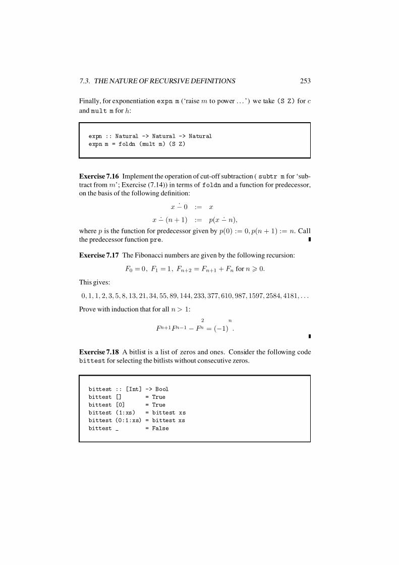
7/16/2019 The Haskell Road to Logic Maths and Programming
http://slidepdf.com/reader/full/the-haskell-road-to-logic-maths-and-programming-5634fa29ef7e9 264/448
7.3. THE NATURE OF RECURSIVE DEFINITIONS 253
Finally, for exponentiation expn m (‘raise m to power . . . ’) we take (S Z) for c
and mult m for h:
expn :: Natural -> Natural -> Natural
expn m = foldn (mult m) (S Z)
Exercise 7.16 Implement the operation of cut-off subtraction ( subtr m for ‘sub-
tract from m’; Exercise (7.14)) in terms of foldn and a function for predecessor,
on the basis of the following definition:
x − 0 := x
x − (n + 1) := p(x − n),
where p is the function for predecessor given by p(0) := 0, p(n + 1) := n. Call
the predecessor function pre.
Exercise 7.17 The Fibonacci numbers are given by the following recursion:
F 0 = 0, F 1 = 1, F n+2 = F n+1 + F n for n 0.
This gives:
0, 1, 1, 2, 3, 5, 8, 13, 21, 34, 55, 89, 144, 233, 377, 610, 987, 1597, 2584, 4181, . . .
Prove with induction that for all n > 1:
F n+1F n−1 − F 2
n = (−1)n
.
Exercise 7.18 A bitlist is a list of zeros and ones. Consider the following code
bittest for selecting the bitlists without consecutive zeros.
bittest :: [Int] -> Bool
bittest [] = True
bittest [0] = True
bittest (1:xs) = bittest xs
bittest (0:1:xs) = bittest xs
bittest _ = False
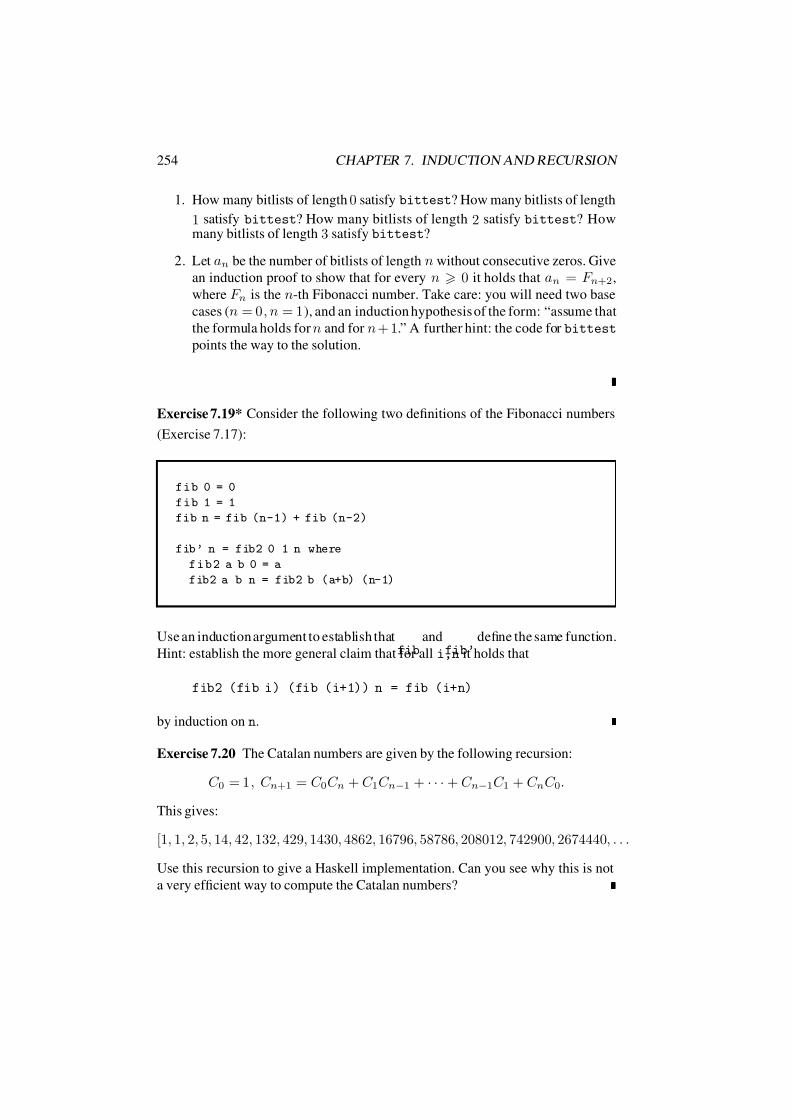
7/16/2019 The Haskell Road to Logic Maths and Programming
http://slidepdf.com/reader/full/the-haskell-road-to-logic-maths-and-programming-5634fa29ef7e9 265/448
254 CHAPTER 7. INDUCTION AND RECURSION
1. How many bitlists of length 0 satisfy bittest? How many bitlists of length
1 satisfy bittest? How many bitlists of length 2 satisfy bittest? Howmany bitlists of length 3 satisfy bittest?
2. Let an be the number of bitlists of length n without consecutive zeros. Give
an induction proof to show that for every n 0 it holds that an = F n+2,
where F n is the n-th Fibonacci number. Take care: you will need two base
cases (n = 0, n = 1), and an induction hypothesis of the form: “assume that
the formula holds for n and for n + 1.” A further hint: the code for bittest
points the way to the solution.
Exercise 7.19* Consider the following two definitions of the Fibonacci numbers
(Exercise 7.17):
fib 0 = 0
fib 1 = 1
fib n = fib (n-1) + fib (n-2)
fib’ n = fib2 0 1 n where
f i b 2 a b 0 = a
fib2 a b n = fib2 b (a+b) (n-1)
Use an induction argument to establish thatfib
andfib’
define the same function.
Hint: establish the more general claim that for all i,n it holds that
fib2 (fib i) (fib (i+1)) n = fib (i+n)
by induction on n.
Exercise 7.20 The Catalan numbers are given by the following recursion:
C 0 = 1, C n+1 = C 0C n + C 1C n−1 + · · · + C n−1C 1 + C nC 0.
This gives:
[1, 1, 2, 5, 14, 42, 132, 429, 1430, 4862, 16796, 58786, 208012, 742900, 2674440, . . .
Use this recursion to give a Haskell implementation. Can you see why this is not
a very efficient way to compute the Catalan numbers?

7/16/2019 The Haskell Road to Logic Maths and Programming
http://slidepdf.com/reader/full/the-haskell-road-to-logic-maths-and-programming-5634fa29ef7e9 266/448
7.4. INDUCTION AND RECURSION OVER TREES 255
Exercise 7.21 Let x0, . . . , xn be a sequence of n + 1 variables. Suppose their
product is to be computed by doing n multiplications. The number of ways todo the multiplications corresponds to the number of bracketings for the sequence.
For instance, if n = 3 there are four variables x0, x1, x2, x3, and five possible
bracketings:
(x1x2)(x3x4), ((x1x2)x3)x4, (x1(x2x3))x4, x1((x2x3)x4), x1(x2(x3x4)).
Show that the number of bracketings for n + 1 variables is given by the Cata-
lan number C n. (Hint: you will need strong induction, so-called because of its
strengthened induction hypothesis. Your induction hypothesis should run: “For
any i with 0 i n, for any sequence of i + 1 variables x0 · · · xi it holds that C igives the number of bracketings for that sequence.”
Example 7.22 Balanced sequences of parentheses of length 2n are defined recur-sively as follows: the empty sequence is balanced; if sequence w is balanced then
(w) is balanced; if sequences w and v are balanced then wv is balanced. Thus,
())(() is not balanced. The balanced sequences involving 3 left and 3 right paren-
theses are:
()()(), (())(), ()(()), (()()), ((())).
There is a one-to-one mapping between bracketings for sequences of n + 1 vari-
ables and balanced sequences of parentheses with 2n parentheses. Let a bracketing
for x0 · · · xn be given. This can be changed into a balanced sequence of parenthe-
ses as follows: We illustrate with the example x0((x2x3)x4).
1. Put one extra pair of parentheses around the bracketing: (x0((x2x3)x4)).
2. Insert multiplication operators at the appropriate places: (x0 ·((x2 ·x3)·x4)).
3. Erase the variables and the left-brackets: ··)·)).
4. Replace the ·’s with left-brackets: (()()).
This mapping gives a one-to-one correspondence between variable bracketings and
balanced parentheses strings, so we get from the previous exercise that there are
C n different balanced parentheses strings of length 2n.
7.4 Induction and Recursion over Trees
Here is a recursive definition of binary trees:

7/16/2019 The Haskell Road to Logic Maths and Programming
http://slidepdf.com/reader/full/the-haskell-road-to-logic-maths-and-programming-5634fa29ef7e9 267/448
256 CHAPTER 7. INDUCTION AND RECURSION
•A single leaf node
•is a binary tree.
• If t1 and t2 are binary trees, then the result of joining t1 and t2 under a single
node (called the root node) is a binary tree. A notation for this is: (• t1 t2)
• Nothing else is a binary tree.
The depth of a binary tree is given by:
• The depth of • is 0.
• The depth of (• t1 t2) is 1+ the maximum of the depths of t1 and t2.
A binary tree is balanced if it either is a single leaf node •, or it has the form
(• t1 t2), with both t1 and t2 balanced, and having the same depth.We see the following: A balanced binary tree of depth 0 is just a single leaf node
•, so its number of nodes is 1. A balanced binary tree of depth 1 has one internal
node and two leaves, so it has 3 nodes. A balanced binary tree of depth 2 has 3internal nodes and 4 leaf nodes, so it has 7 nodes. A binary tree of depth 3 has 7internal nodes plus 8 leaf nodes, so it has 15 nodes.
Recursion and induction over binary trees are based on two cases t = • and t =(• t1 t2).
Example 7.23 Suppose we want to find a formula for the number of nodes in a
balanced binary tree of depth d.
q q q q
q q q q q q
q q q q q q q q
qq qq qq qq
Suppose we want to show in general that the number of nodes of a binary tree of
depth n is 2n+1 − 1. Then a proof by mathematical induction is in order. We
proceed as follows:
Basis If n = 0, then 2n+1 − 1 = 21 − 1 = 1. This is indeed the number of nodes
of a binary tree of depth 0.
Induction step Assume the number of nodes of a binary tree of depth n is 2n+1
−1. We have to show that the number of nodes of a binary tree of depth n + 1equals 2n+2 − 1.

7/16/2019 The Haskell Road to Logic Maths and Programming
http://slidepdf.com/reader/full/the-haskell-road-to-logic-maths-and-programming-5634fa29ef7e9 268/448
7.4. INDUCTION AND RECURSION OVER TREES 257
A binary tree of depth n + 1 can be viewed as a set of internal nodes con-
stituting a binary tree of depth n, plus a set of leaf nodes, consisting of twonew leaf nodes for every old leaf node from the tree of depth n. By induc-
tion hypothesis, we know that a tree of depth n has 2n+1 − 1 nodes, so a
tree of depth n + 1 has 2n+1 − 1 internal nodes. It is easy to see that a tree
of depth n + 1 has 2n+1 leaf nodes. The total number of nodes of a tree of
depth n + 2 is therefore 2n+1 − 1 + 2n+1 = 2 · 2n+1 − 1 = 2n+2 − 1, and
we have proved our induction step.
To illustrate trees and tree handling a bit further, here is a Haskell definition of
binary trees, with a procedure for making balanced trees of an arbitrary depth n,
and a procedure for counting their nodes in a naive way.
We use L for a single leaf •. The data declaration specifies that a BinTree either
is an object L (a single leaf), or an object constructed by applying the constructor
N to two BinTree objects (the result of constructing a new binary tree (• t1 t2)from two binary trees t1 and t2).
The addition deriving Show ensures that data of this type can be displayed on
the screen.
data BinTree = L | N BinTree BinTree deriving Show
makeBinTree :: Integer -> BinTree
makeBinTree 0 = L makeBinTree (n + 1) = N (makeBinTree n) (makeBinTree n)
count :: BinTree -> Integer
count L = 1
count (N t1 t2) = 1 + count t1 + count t2
With this code you can produce binary trees as follows:
IAR> makeBinTree 6
N (N (N (N (N (N L L) (N L L)) (N (N L L) (N L L))) (N (N (N L L) (N
L L)) (N (N L L) (N L L)))) (N (N (N (N L L) (N L L)) (N (N L L) (N L
L))) (N (N (N L L) (N L L)) (N (N L L) (N L L))))) (N (N (N (N (N L L)(N L L)) (N (N L L) (N L L))) (N (N (N L L) (N L L)) (N (N L L) (N L
L)))) (N (N (N (N L L) (N L L)) (N (N L L) (N L L))) (N (N (N L L) (N

7/16/2019 The Haskell Road to Logic Maths and Programming
http://slidepdf.com/reader/full/the-haskell-road-to-logic-maths-and-programming-5634fa29ef7e9 269/448
258 CHAPTER 7. INDUCTION AND RECURSION
L L)) (N (N L L) (N L L)))))
IAR>
If you want to check that the depth of a the result of maketree 6 is indeed 6,
or that maketree 6 is indeed balanced, here are some procedures. Note that the
procedures follow the definitions of depth and balanced to the letter:
depth :: BinTree -> Integer
depth L = 0
depth (N t1 t2) = (max (depth t1) (depth t2)) + 1
balanced :: BinTree -> Bool
balanced L = True
balanced (N t1 t2) = (balanced t1)
&& (balanced t2)
&& depth t1 == depth t2
The programs allow us to check the relation between count (makeBinTree n)and 2^(n+1) - 1 for individual values of n:
IAR> count (makeBinTree 6) == 2^7 - 1True
What the proof by mathematical induction provides is an insight that the relation
holds in general. Mathematical induction does not give as clue as to how to find a
formula for the number of nodes in a tree. It only serves as a method of proof once
such a formula is found.
So how does one find a formula for the number of nodes in a binary tree in the
first place? By noticing how such trees grow. A binary tree of depth 0 has 1 node,
and this node is a leaf node. This leaf grows two new nodes, so a binary tree of
depth 1 has 1+ 2 = 3 nodes. In the next step the 2 leaf nodes grow two new nodes
each, so we get 22 = 4 new leaf nodes, and the number of nodes of a binary tree
of depth 2 equals 1 + 2 + 4 = 7. In general, a tree of depth n−
1 is transformed
into one of depth n by growing 2n new leaves, and the total number of leaves of
the new tree is given by 20 + 21 + · · · + 2n. In other words, the number of nodes
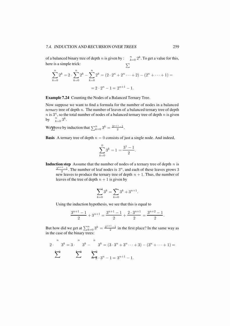
7/16/2019 The Haskell Road to Logic Maths and Programming
http://slidepdf.com/reader/full/the-haskell-road-to-logic-maths-and-programming-5634fa29ef7e9 270/448
7.4. INDUCTION AND RECURSION OVER TREES 259
of a balanced binary tree of depth n is given by : nk=0 2k. To get a value for this,
here is a simple trick:
nk=0
2k = 2 ·nk=0
2k −nk=0
2k = (2 · 2n + 2n · · · + 2) − (2n + · · · + 1) =
= 2 · 2n − 1 = 2n+1 − 1.
Example 7.24 Counting the Nodes of a Balanced Ternary Tree.
Now suppose we want to find a formula for the number of nodes in a balanced
ternary tree of depth n. The number of leaves of a balanced ternary tree of depth
n is 3n, so the total number of nodes of a balanced ternary tree of depth n is given
by nk=0 3k.
We prove by induction thatn
k=0 3k = 3n+1−12
.
Basis A ternary tree of depth n = 0 consists of just a single node. And indeed,
0k=0
3k = 1 =31 − 1
2.
Induction step Assume that the number of nodes of a ternary tree of depth n is3n+1−1
2 . The number of leaf nodes is 3n, and each of these leaves grows 3new leaves to produce the ternary tree of depth n + 1. Thus, the number of
leaves of the tree of depth n + 1 is given by
n+1k=0
3k =nk=0
3k + 3n+1.
Using the induction hypothesis, we see that this is equal to
3n+1 − 1
2+ 3n+1 =
3n+1 − 1
2+
2 · 3n+1
2=
3n+2 − 1
2.
But how did we get atn
k=0 3k = 3n+1−12 in the first place? In the same way as
in the case of the binary trees:
2 ·n
k=0
3k = 3 ·n
k=0
3k −n
k=0
3k = (3 · 3n + 3n · · · + 3) − (3n + · · · + 1) =
= 3 · 3n − 1 = 3n+1 − 1.

7/16/2019 The Haskell Road to Logic Maths and Programming
http://slidepdf.com/reader/full/the-haskell-road-to-logic-maths-and-programming-5634fa29ef7e9 271/448
260 CHAPTER 7. INDUCTION AND RECURSION
Therefore
nk=0
3k = 3n+1 − 12
.
Exercise 7.25 Write a Haskell definition of ternary trees, plus procedures for gen-
erating balanced ternary trees and counting their node numbers.
Example 7.26 Counting the Nodes of a Balanced m-ary Tree. The number of
nodes of a balanced m-ary tree of depth n (with m > 1) is given byn
k=0 mk =mn+1−1m−1 . Here is a proof by mathematical induction.
Basis An m-ary tree of depth 0 consists of just a single node. In fact, 0k=0 mk =
1 =m
−1
m−1 .Induction step Assume that the number of nodes of an m-ary tree of depth n is
mn+1−1m−1
. The number of leaf nodes is mn, and each of these leaves grows
m new leaves to produce the ternary tree of depth n + 1. Thus, the number
of leaves of the tree of depth n + 1 is given by
n+1k=0
mk =nk=0
mk + mn+1.
Using the induction hypothesis, we see that this is equal to
mn+1 − 1
m − 1+ mn+1 =
mn+1 − 1
m − 1+
mn+2 − mn+1
m − 1=
mn+2 − 1
m − 1.
Note that the proofs by mathematical induction do not tell you how to find the for-
mulas for which the induction proof works in the first place. This is an illustration
of the fact that mathematical induction is a method of verification, not a method of
invention. Indeed, mathematical induction is no replacement for the use of creative
intuition in the process of finding meaningful relationships in mathematics.
Exercise 7.27 Geometric Progressions.
Prove by mathematical induction (assuming q = 1, q = 0):
n
k=0
q k =q n+1 − 1
q −
1.
Note that this exercise is a further generalization of Example 7.26.
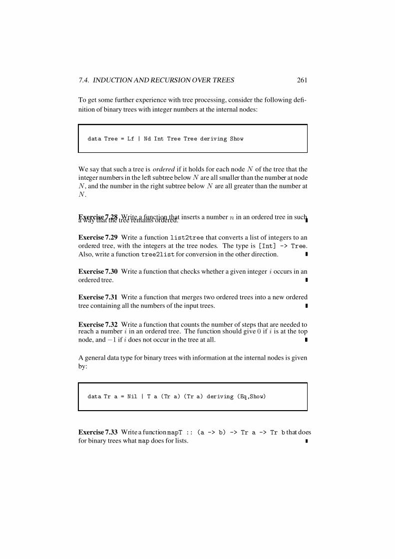
7/16/2019 The Haskell Road to Logic Maths and Programming
http://slidepdf.com/reader/full/the-haskell-road-to-logic-maths-and-programming-5634fa29ef7e9 272/448
7.4. INDUCTION AND RECURSION OVER TREES 261
To get some further experience with tree processing, consider the following defi-
nition of binary trees with integer numbers at the internal nodes:
data Tree = Lf | Nd Int Tree Tree deriving Show
We say that such a tree is ordered if it holds for each node N of the tree that the
integer numbers in the left subtree below N are all smaller than the number at node
N , and the number in the right subtree below N are all greater than the number at
N .
Exercise 7.28 Write a function that inserts a number n in an ordered tree in sucha way that the tree remains ordered.
Exercise 7.29 Write a function list2tree that converts a list of integers to an
ordered tree, with the integers at the tree nodes. The type is [Int] -> Tree.
Also, write a function tree2list for conversion in the other direction.
Exercise 7.30 Write a function that checks whether a given integer i occurs in an
ordered tree.
Exercise 7.31 Write a function that merges two ordered trees into a new ordered
tree containing all the numbers of the input trees.
Exercise 7.32 Write a function that counts the number of steps that are needed toreach a number i in an ordered tree. The function should give 0 if i is at the top
node, and −1 if i does not occur in the tree at all.
A general data type for binary trees with information at the internal nodes is given
by:
data Tr a = Nil | T a (Tr a) (Tr a) deriving (Eq,Show)
Exercise 7.33 Write a function mapT :: (a -> b) -> Tr a -> Tr b that does
for binary trees what map does for lists.

7/16/2019 The Haskell Road to Logic Maths and Programming
http://slidepdf.com/reader/full/the-haskell-road-to-logic-maths-and-programming-5634fa29ef7e9 273/448
262 CHAPTER 7. INDUCTION AND RECURSION
Exercise 7.34 Write a function
foldT :: (a -> b -> b -> b) -> b -> (Tr a) -> b
that does for binary trees what foldn does for naturals.
Exercise 7.35 Conversion of a tree into a list can be done in various ways, de-
pending on when the node is visited:
Preorder traversal of a tree is the result of first visiting the node, next visiting
the left subtree, and finally visiting the right subtree.
Inorder traversal of a tree is the result of first visiting the left subtree, next visit-
ing the node, and finally visiting the right subtree.
Postorder traversal of a tree is the result of first visiting the left subtree, next
visiting the right subtree, and finally visiting the node.
Define these three conversion functions from trees to lists in terms of the foldT
function from Exercise 7.34.
Exercise 7.36 An ordered tree is a tree with information at the nodes given in
such manner that the item at a node must be bigger than all items in the left sub-
tree and smaller than all items in the right subtree. A tree is ordered iff the list
resulting from its inorder traversal is ordered and contains no duplicates. Give an
implementation of this check.
Exercise 7.37 An ordered tree (Exercise 7.36) can be used as a dictionary by
putting items of of type (String,String) at the internal nodes, and defining
the ordering as: (v, w) (v, w) iff v v. Dictionaries get the following type:
type Dict = Tr (String,String)
Give code for looking up a word definition in a dictionary. The type declaration is:
lookupD :: String -> Dict -> [String]

7/16/2019 The Haskell Road to Logic Maths and Programming
http://slidepdf.com/reader/full/the-haskell-road-to-logic-maths-and-programming-5634fa29ef7e9 274/448
7.4. INDUCTION AND RECURSION OVER TREES 263
If (v, w) occurs in the dictionary, the call lookupD v d should yield [w], other-
wise []. Use the order on the dictionary tree.
Exercise 7.38 For efficient search in an ordered tree (Exercises 7.36 and 7.37) it
is crucial that the tree is balanced: the left and right subtree should have (nearly)
the same depth and should themselves be balanced.
The following auxiliary function splits non-empty lists into parts of (roughly)
equal lengths.
split :: [a] -> ([a],a,[a])
split xs = (ys1,y,ys2)
where
ys1 = take n xs(y:ys2) = drop n xs
n = length xs ‘div‘ 2
Use this to implement a function buildTree :: [a] -> Tr a for transforming
an ordered list into an ordered and balanced binary tree.
Here is a data type LeafTree for binary leaf trees (binary trees with information
at the leaf nodes):
data LeafTree a = Leaf a| Node (LeafTree a) (LeafTree a) deriving Show
Here is an example leaf tree:
ltree :: LeafTree String
ltree = Node
(Leaf "I")
(Node
(Leaf "love")
(Leaf "you"))
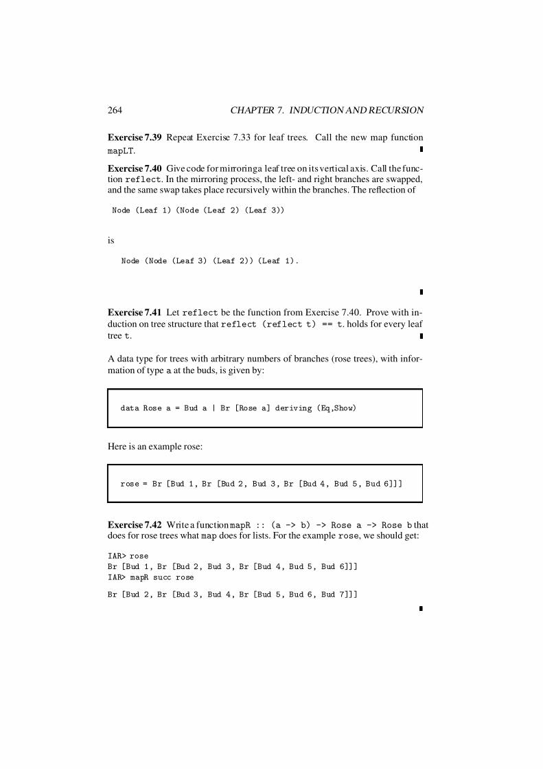
7/16/2019 The Haskell Road to Logic Maths and Programming
http://slidepdf.com/reader/full/the-haskell-road-to-logic-maths-and-programming-5634fa29ef7e9 275/448
264 CHAPTER 7. INDUCTION AND RECURSION
Exercise 7.39 Repeat Exercise 7.33 for leaf trees. Call the new map function
mapLT.
Exercise 7.40 Give code for mirroringa leaf tree on its vertical axis. Call the func-tion reflect. In the mirroring process, the left- and right branches are swapped,and the same swap takes place recursively within the branches. The reflection of
Node (Leaf 1) (Node (Leaf 2) (Leaf 3))
is
Node (Node (Leaf 3) (Leaf 2)) (Leaf 1).
Exercise 7.41 Let reflect be the function from Exercise 7.40. Prove with in-
duction on tree structure that reflect (reflect t) == t. holds for every leaf
tree t.
A data type for trees with arbitrary numbers of branches (rose trees), with infor-
mation of type a at the buds, is given by:
data Rose a = Bud a | Br [Rose a] deriving (Eq,Show)
Here is an example rose:
rose = Br [Bud 1, Br [Bud 2, Bud 3, Br [Bud 4, Bud 5, Bud 6]]]
Exercise 7.42 Write a function mapR :: (a -> b) -> Rose a -> Rose b thatdoes for rose trees what map does for lists. For the example rose, we should get:
IAR> rose
Br [Bud 1, Br [Bud 2, Bud 3, Br [Bud 4, Bud 5, Bud 6]]]
IAR> mapR succ rose
Br [Bud 2, Br [Bud 3, Bud 4, Br [Bud 5, Bud 6, Bud 7]]]

7/16/2019 The Haskell Road to Logic Maths and Programming
http://slidepdf.com/reader/full/the-haskell-road-to-logic-maths-and-programming-5634fa29ef7e9 276/448
7.5. INDUCTION AND RECURSION OVER LISTS 265
7.5 Induction and Recursion over Lists
Induction and recursion over natural numbers are based on the two cases n = 0and n = k + 1. Induction and recursion over lists are based on the two cases
l = [] and l = x:xs, where x is an item and xs is the tail of the list. An example
is the definition of a function len that gives the length of a list. In fact, Haskell
has a predefined function length for this purpose; our definition of len is just for
purposes of illustration.
len [] = 0
len (x:xs) = 1 + len xs
Similarly, Haskell has a predefined operation ++ for concatenation of lists. For
purposes of illustration we repeat our version from Section (4.8).
cat :: [a] -> [a] -> [a]
cat [] ys = ys
cat (x:xs) ys = x : (cat xs ys)
As an example of an inductive proof over lists, we show that concatenation of listsis associative.
Proposition 7.43 For all lists xs, ys and zs over the same type a:
cat (cat xs ys) zs = cat xs (cat ys zs) .
Proof. Induction on xs.
Basis
cat (cat [] ys) zscat.1
= cat ys zscat.1= cat [] (cat ys zs).
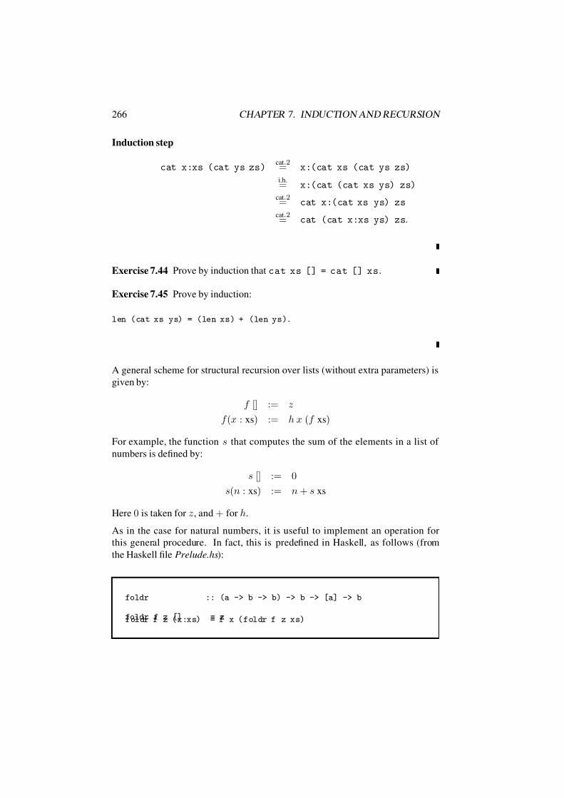
7/16/2019 The Haskell Road to Logic Maths and Programming
http://slidepdf.com/reader/full/the-haskell-road-to-logic-maths-and-programming-5634fa29ef7e9 277/448
266 CHAPTER 7. INDUCTION AND RECURSION
Induction step
cat x:xs (cat ys zs)cat.2= x:(cat xs (cat ys zs)
i.h.= x:(cat (cat xs ys) zs)
cat.2= cat x:(cat xs ys) zs
cat.2= cat (cat x:xs ys) zs.
Exercise 7.44 Prove by induction that cat xs [] = cat [] xs.
Exercise 7.45 Prove by induction:
len (cat xs ys) = (len xs) + (len ys).
A general scheme for structural recursion over lists (without extra parameters) is
given by:
f [] := z
f (x : xs) := h x (f xs)
For example, the function s that computes the sum of the elements in a list of
numbers is defined by:
s [] := 0
s(n : xs) := n + s xs
Here 0 is taken for z, and + for h.
As in the case for natural numbers, it is useful to implement an operation for
this general procedure. In fact, this is predefined in Haskell, as follows (from
the Haskell file Prelude.hs):
foldr :: (a -> b -> b) -> b -> [a] -> b
foldr f z [] = zfoldr f z (x:xs) = f x (foldr f z xs)

7/16/2019 The Haskell Road to Logic Maths and Programming
http://slidepdf.com/reader/full/the-haskell-road-to-logic-maths-and-programming-5634fa29ef7e9 278/448
7.5. INDUCTION AND RECURSION OVER LISTS 267
In general, z is the identity element of the operation f, i.e., the value you would
start out with in the base case of a recursive definition of the operation. The identityelement for addition is 0, for multiplication it is 1 (see Section 7.3).
The base clause of the definition of foldr says that if you want to fold an empty
list for operation f, the result is the identity element for f. The recursive clause
says that to fold a non-empty list for f, you perform f to its first element and to
the result of folding the remainder of the list for f.
The following informal version of the definition of foldr may further clarify its
meaning:
foldr (⊕) z [x1, x2, . . . , xn] := x1 ⊕ (x2 ⊕ (· · · (xn ⊕ z) · · · )).
The function add :: [Natural] -> Natural can now be defined as:
add = foldr plus Z
The function mlt :: [Natural] -> Natural is given by:
mlt = foldr mult (S Z)
And here is an alternative definition of list length, with values of type Natural.
Note that the function ( \ _ n - > S n ) ignores its first argument (you don’t have
to look at the items in a list in order to count them) and returns the successor of
its second argument (for this second argument represents the number of items that
were counted so far).
ln :: [a] -> Natural
ln = foldr (\ _ n -> S n) Z
It is also possible to use foldr on the standard type for integers. Computing theresult of adding or multiplying all elements of a list of integers can be done asfollows:

7/16/2019 The Haskell Road to Logic Maths and Programming
http://slidepdf.com/reader/full/the-haskell-road-to-logic-maths-and-programming-5634fa29ef7e9 279/448
268 CHAPTER 7. INDUCTION AND RECURSION
Prelude> foldr (+) 0 [1..10]
55Prelude> foldr (*) 1 [1..10]
3628800
Exercise 7.46 Use foldr to give a new implementation of generalized union and
foldr1 to give a new implementation of generalized intersection for lists. (Look
up the code for foldr1 in the Haskell prelude. Compare Exercise 4.53.)
Consider the following definitions of generalized conjunction and disjunction:
or :: [Bool] -> Bool
or [] = False
or (x:xs) = x || or xs
and :: [Bool] -> Bool
and [] = True
and (x:xs) = x && and xs
The function or takes a list of truth values and returns True if at least one member
of the list equals True, while and takes a list of truth values and returns True if
all members of the list equal True. (We have encountered and before, in Section
2.2.)
In fact, Haskell has predefined these operations, in terms of foldr. To see how
we can use foldr to implement generalized conjunction and disjunction, we onlyneed to know what the appropriate identity elements of the operations are. Should
the conjunction of all elements of [] count as true or false? As true, for it is indeed
(trivially) the case that all elements of [] are true. So the identity element for
conjunction is True. Should the disjunction of all elements of [] count as true or
false? As false, for it is false that [] contains an element which is true. Therefore,
the identity element for disjunction is False. This explains the following Haskell
definition in Prelude.hs:
and, or :: [Bool] -> Bool
and = foldr (&&) True
or = foldr (||) False

7/16/2019 The Haskell Road to Logic Maths and Programming
http://slidepdf.com/reader/full/the-haskell-road-to-logic-maths-and-programming-5634fa29ef7e9 280/448
7.5. INDUCTION AND RECURSION OVER LISTS 269
Exercise 7.47 Define a function srt that sorts a list of items in class Ord a by
folding the list with a function insrt.
The operation foldr folds ‘from the right’. Folding ‘from the left’ can be done
with its cousin foldl, predefined in Prelude.hs as follows:
foldl :: (a -> b -> a) -> a -> [b] -> a
foldl f z [] = z
foldl f z (x:xs) = foldl f (f z x) xs
An informal version may further clarify this:
foldl (⊕) z [x1, x2, . . . , xn] := (· · · ((z ⊕ x1) ⊕ x2) ⊕ · · · ) ⊕ xn.
This can be used to flesh out the following recursion scheme:
f z [] := z
f z (x : xs) := f (h z x) xs
This boils down to recursion over lists with an extra parameter, and in fact foldl
can be used to speed up list processing. The case of reversing a list is an example:
r zs [] := zs
r zs (x : xs) := r (prefix zs x) xs,
where prefix is given by prefix ys y = y:ys. Here is a definition in terms of
foldl:
rev = foldl (\ xs x -> x:xs) []
The list [1,2,3] is reversed as follows:
rev [1,2,3] = foldl (\ xs x -> x:xs) [] [1,2,3]
= foldl (\ xs x -> x:xs) ((\ xs x -> x:xs) [] 1) [2,3]= foldl (\ xs x -> x:xs) [1] [2,3]
= foldl (\ xs x -> x:xs) ((\ xs x -> x:xs) [1] 2) [3]

7/16/2019 The Haskell Road to Logic Maths and Programming
http://slidepdf.com/reader/full/the-haskell-road-to-logic-maths-and-programming-5634fa29ef7e9 281/448
270 CHAPTER 7. INDUCTION AND RECURSION
= foldl (\ xs x -> x:xs) [2,1] [3]
= foldl (\ xs x -> x:xs) ((\ xs x -> x:xs) [2,1] 3) []= foldl (\ xs x -> x:xs) [3,2,1] []
= [3,2,1]
Note that (\ xs x -> x:xs) has type [a] -> a -> [a]. An alternative defi-nition of rev, in terms of foldr, would need a swap function
\ x xs -> xs ++ [x] :: a -> [a] -> [a]
and would be much less efficient:
rev’ = foldr (\ x xs -> xs ++ [x]) []
The inefficiency resides in the fact that ++ itself is defined recursively, as follows:
[] ++ ys = ys
(x:xs) ++ ys = x : (xs ++ ys)
To see why rev’ is less efficient than rev, look at the following, where we write
postfix for (\ x xs -> xs ++[x]).
rev’ [1,2,3] = foldr postfix [] [1,2,3]
= postfix 1 (foldr postfix [] [2,3])
= (foldr postfix [] [2,3]) ++ [1]
= (postfix 2 (foldr postfix [] [3])) ++ [1]
= (foldr postfix [] [3]) ++ [2] ++ [1]
= (postfix 3 (foldr postfix [] [])) ++ [2] ++ [1]
= (foldr postfix [] []) ++ [3] ++ [2] ++ [1]
= [] ++ [3] ++ [2] ++ [1]
= ([3] ++ [2]) ++ [1]
= 3:([] ++ [2]) ++ [1]
= [3,2] ++ [1]
= 3:([2] ++ [1])= 3:2:([] ++ [1])
= [3,2,1]
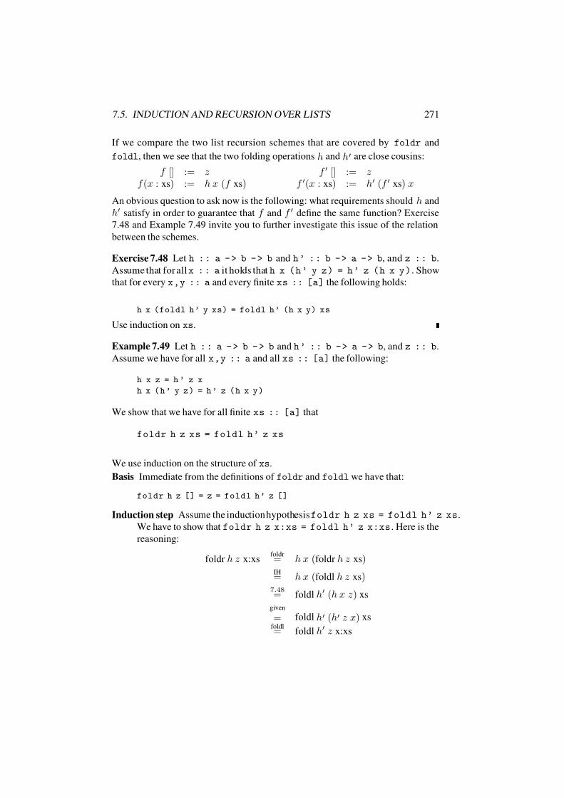
7/16/2019 The Haskell Road to Logic Maths and Programming
http://slidepdf.com/reader/full/the-haskell-road-to-logic-maths-and-programming-5634fa29ef7e9 282/448
7.5. INDUCTION AND RECURSION OVER LISTS 271
If we compare the two list recursion schemes that are covered by foldr and
foldl, then we see that the two folding operations h and h are close cousins:
f [] := z f [] := zf (x : xs) := h x (f xs) f (x : xs) := h (f xs) x
An obvious question to ask now is the following: what requirements should h and
h satisfy in order to guarantee that f and f define the same function? Exercise
7.48 and Example 7.49 invite you to further investigate this issue of the relation
between the schemes.
Exercise 7.48 Let h : : a - > b - > b and h ’ : : b - > a - > b, and z : : b.
Assume that for all x : : a it holds that h x ( h ’ y z ) = h ’ z ( h x y ). Show
that for every x,y :: a and every finite xs :: [a] the following holds:
h x (foldl h’ y xs) = foldl h’ (h x y) xs
Use induction on xs.
Example 7.49 Let h : : a - > b - > b and h ’ : : b - > a - > b, and z : : b.
Assume we have for all x,y :: a and all xs :: [a] the following:
h x z = h ’ z x
h x ( h ’ y z ) = h ’ z ( h x y )
We show that we have for all finite xs :: [a] that
foldr h z xs = foldl h’ z xs
We use induction on the structure of xs.
Basis Immediate from the definitions of foldr and foldl we have that:
foldr h z [] = z = foldl h’ z []
Induction step Assume the induction hypothesis foldr h z xs = foldl h’ z xs.
We have to show that foldr h z x:xs = foldl h’ z x:xs . Here is the
reasoning:
foldr h z x:xsfoldr= h x (foldr h z xs)IH= h x (foldl h z xs)
7.48= foldl h (h x z) xs
given
= foldl h (h z x) xsfoldl= foldl h z x:xs

7/16/2019 The Haskell Road to Logic Maths and Programming
http://slidepdf.com/reader/full/the-haskell-road-to-logic-maths-and-programming-5634fa29ef7e9 283/448
272 CHAPTER 7. INDUCTION AND RECURSION
For an application of Example (7.49), note that the functions postfix and prefixare related by:
postfix x [] = [] ++ [x] = [x] == prefix [] x
postfix x (prefix xs y) = (prefix xs y) ++ [x]
= y:(xs ++ [x])
= y:(postfix x xs)
= prefix (postfix x xs) y
It follows from this and the result of the example that rev and rev’ indeed com-
pute the same function.
Exercise 7.50 Consider the following version of rev.
rev1 :: [a] -> [a]
rev1 xs = rev2 xs []
where
rev2 [] ys = ys
rev2 (x:xs) ys = rev2 xs (x:ys)
Which version is more efficient, the original rev, the version rev’, or this version?
Why?
Exercise 7.51 Define an alternative version ln’ of ln using foldl instead of
foldr.
In Section 1.8 you got acquainted with the map and filter functions. The twooperations map and filter can be combined:
Prelude> filter (>4) (map (+1) [1..10])
[5,6,7,8,9,10,11]
Prelude> map (+1) (filter (>4) [1..10])
[6,7,8,9,10,11]
These outcomes are different. This is because the test (>4) yields a different resultafter all numbers are increased by 1. When we make sure that the test used in thefilter takes this change into account, we get the same answers:

7/16/2019 The Haskell Road to Logic Maths and Programming
http://slidepdf.com/reader/full/the-haskell-road-to-logic-maths-and-programming-5634fa29ef7e9 284/448
7.6. SOME VARIATIONS ON THE TOWER OF HANOI 273
Prelude> filter (>4) (map (+1) [1..10])
[5,6,7,8,9,10,11]Prelude> map (+1) (filter ((>4).(+1)) [1..10])
[5,6,7,8,9,10,11]
Here (f . g) denotes the result of first applying g and next f. Note: ((>4).(+1))
defines the same property as (>3). Exercise 7.52 gives you an opportunity to show
that these identical answers are no accident.
Exercise 7.52 Let xs :: [a], let f : : a - > b, and let p :: b -> Bool be a
total predicate. Show that the following holds:
filter p (map f xs) = map f (filter ( p · f ) xs).
Note: a predicate p :: b -> Bool is total if for every object x : : b, the appli-
cation p x gives either true or false. In particular, for no x : : b does p x raisean error.
7.6 Some Variations on the Tower of Hanoi
Figure 7.1: The Tower of Hanoi.
The Tower of Hanoi is a tower of 8 disks of different sizes, stacked in order of
decreasing size on a peg. Next to the tower, there are two more pegs. The task is
to transfer the whole stack of disks to one of the other pegs (using the third peg
as an auxiliary) while keeping to the following rules: (i) move only one disk at a
time, (ii) never place a larger disk on top of a smaller one.
Exercise 7.53 In this exercise, you are required to invent your own solution, and
next prove it by mathematical induction. Make sure that the reasoning also es-
tablishes that the formula you find for the number of moves is the best one can
do.

7/16/2019 The Haskell Road to Logic Maths and Programming
http://slidepdf.com/reader/full/the-haskell-road-to-logic-maths-and-programming-5634fa29ef7e9 285/448
274 CHAPTER 7. INDUCTION AND RECURSION
1. How many moves does it take to completely transfer a tower consisting of n
disks?
2. Prove by mathematical induction that your answer to the previous question
is correct.
3. How many moves does it take to completely transfer the tower of Hanoi?
Exercise 7.54 Can you also find a formula for the number of moves of the disk of
size k during the transfer of a tower with disks of sizes 1, . . . , n, and 1 k n?Again, you should prove by mathematical induction that your formula is correct.
According to legend, there exists a much larger tower than the tower of Hanoi, the
tower of Brahma, with 64 disks. Monks are engaged in transferring the disks of
the Tower of Brahma, from the beginning of the universe to the present day. As
soon as they will have completed their task the tower will crumble and the world
will end.
Exercise 7.55 How long will the universe last, given that the monks move one
disk per day?
For an implementation of the disk transfer procedure, an obvious way to represent
the starting configurationof the tower of Hanoi is ([1,2,3,4,5,6,7,8],[],[]).
For clarity, we give the three pegs names A, B and C. and we declare a type Tower:
data Peg = A | B | C
type Tower = ([Int], [Int], [Int])
There are six possible single moves from one peg to another:

7/16/2019 The Haskell Road to Logic Maths and Programming
http://slidepdf.com/reader/full/the-haskell-road-to-logic-maths-and-programming-5634fa29ef7e9 286/448
7.6. SOME VARIATIONS ON THE TOWER OF HANOI 275
IAR> (display 88 . show . take 200 . hanoi) 8[([1,2,3,4,5,6,7,8],[],[]),([2,3,4,5,6,7,8],[1],[]),([3,4,5,6,7,8],[1],[2]),([3,4,5,6,7,8],[],[1,2]),([4,5,6,7,8],[3],[1,2]),([1,4,5,6,7,8],[3],[2]),([1,4,5,6,7,8],[2,3],[]),([4,5,6,7,8],[1,2,3],[]),([5,6,7,8],[1,2,3],[4]),([5,6,7,8],[2,3],[1,4]),([2,5,6,7,8],[3],[1,4]),([1,2,5,6,7,8],[3],[4]),([1,2,5,6,7,8],[],[3,4]),([2,5,6,7,8],[1],[3,4]),([5,6,7,8],[1],[2,3,4]),([5,6,7,8],[],[1,2,3,4]),([6,7,8],[5],[1,2,3,4]),([1,6,7,8],[5],[2,3,4]),([1,6,7,8],[2,5],[3,4]),([6,7,8],[1,2,5],[3,4]),([3,6,7,8],[1,2,5],[4]),([3,6,7,8],[2,5],[1,4]),([2,3,6,7,8],[5],[1,4]),([1,2,3,6,7,8],[5],[4]),([1,2,3,6,7,8],[4,5],[]),([2,3,6,7,8],[1,4,5],[]),([3,6,7,8],[1,4,5],[2]),([3,6,7,8],[4,5],[1,2]),([6,7,8],[3,4,5],[1,2]),([1,6,7,8],[3,4,5],[2]),([1,6,7,8],[2,3,4,5],[]),([6,7,8],[1,2,3,4,5],[]),([7,8],[1,2,3,4,5],[6]),([7,8],[2,3,4,5],[1,6]),([2,7,8],[3,4,5],[1,6]),([1,2,7,8],[3,4,5],[6]),([1,2,7,8],[4,5],[3,6]),([2,7,8],[1,4,5],[3,6]),([7,8],[1,4,5],[2,3,6]),([7,8],[4,5],[1,2,3,6]),([4,7,8],[5],[1,2,3,6]),([1,4,7,8],[5],[2,3,6]),([1,4,7,8],[2,5],[3,6]),([4,7,8],[1,2,5],[3,6]),([3,4,7,8],[1,2,5],[6]),([3,4,7,8],[2,5],[1,6]),([2,3,4,7,8],[5],[1,6]),([1,2,3,4,7,8],[5],[6]),([1,2,3,4,7,8],[],[5,6]),([2,3,4,7,8],[1],[5,6]),([3,4,7,8],[1],[2,5,6]),([3,4,7,8],[],[1,2,5,6]),([4,7,8],[3],[1,2,5,6]),([1,4,7,8],[3],[2,5,6]),([1,4,7,8],[2,3],[5,6]),([4,7,8],[1,2,3],[5,6]),([7,8],[1,2,3],[4,5,6]),([7,8],[2,3],[1,4,5,6]),([2,7,8],[3],[1,4,5,6]),([1,2,7,8],[3],[4,5,6]),([1,2,7,8],[],[3,4,5,6]),([2,7,8],[1],[3,4,5,6]),([7,8],[1],[2,3,4,5,6]),([7,8],[],[1,2,3,4,5,6]),([8],[7],[1,2,3,4,5,6]),([1,8],[7],[2,3,4,5,6]),([1,8],[2,7],[3,4,5,6]),([8],[1,2,7],[3,4,5,6]),([3,8],[1,2,7],[4,5,6])
,([3,8],[2,7],[1,4,5,6]),([2,3,8],[7],[1,4,5,6]),([1,2,3,8],[7],[4,5,6]),([1,2,3,8],[4,7],[5,6]),([2,3,8],[1,4,7],[5,6]),([3,8],[1,4,7],[2,5,6]),([3,8],[4,7],[1,2,5,6]),([8],[3,4,7],[1,2,5,6]),([1,8],[3,4,7],[2,5,6]),([1,8],[2,3,4,7],[5,6]),([8],[1,2,3,4,7],[5,6]),([5,8],[1,2,3,4,7],[6]),([5,8],[2,3,4,7],[1,6]),([2,5,8],[3,4,7],[1,6]),([1,2,5,8],[3,4,7],[6]),([1,2,5,8],[4,7],[3,6]),([2,5,8],[1,4,7],[3,6]),([5,8],[1,4,7],[2,3,6]),([5,8],[4,7],[1,2,3,6]),([4,5,8],[7],[1,2,3,6]),([1,4,5,8],[7],[2,3,6]),([1,4,5,8],[2,7],[3,6]),([4,5,8],[1,2,7],[3,6]),([3,4,5,8],[1,2,7],[6]),([3,4,5,8],[2,7],[1,6]),([2,3,4,5,8],[7],[1,6]),([1,2,3,4,5,8],[7],[6]),([1,2,3,4,5,8],[6,7],[]),([2,3,4,5,8],[1,6,7],[]),([3,4,5,8],[1,6,7],[2]),([3,4,5,8],[6,7],[1,2]),([4,5,8],[3,6,7],[1,2]),([1,4,5,8],[3,6,7],[2]),([1,4,5,8],[2,3,6,7],[]),([4,5,8],[1,2,3,6,7],[]),([5,8],[1,2,3,6,7],[4]),([5,8],[2,3,6,7],[1,4]),([2,5,8],[3,6,7],[1,4]),([1,2,5,8],[3,6,7],[4]),([1,2,5,8],[6,7],[3,4]),([2,5,8],[1,6,7],[3,4]),([5,8],[1,6,7],[2,3,4]),([5,8],[6,7],[1,2,3,4]),([8],[5,6,7],[1,2,3,4]),([1,8],[5,6,7],[2,3,4]),([1,8],[2,5,6,7],[3,4]),([8],[1,2,5,6,7],[3,4]),([3,8],[1,2,5,6,7],[4]),([3,8],[2,5,6,7],[1,4]),([2,3,8],[5,6,7],[1,4]),([1,2,3,8],[5,6,7],[4]),([1,2,3,8],[4,5,6,7],[]),([2,3,8],[1,4,5,6,7],[]),([3,8],[1,4,5,6,7],[2]),([3,8],[4,5,6,7],[1,2]),([8],[3,4,5,6,7],[1,2]),([1,8],[3,4,5,6,7],[2]),([1,8],[2,3,4,5,6,7],[]),([8],[1,2,3,4,5,6,7],[]),([],[1,2,3,4,5,6,7],[8]),([],[2,3,4,5,6,7],[1,8]),([2],[3,4,5,6,7],[1,8]),([1,2],[3,4,5,6,7],[8]),([1,2],[4,5,6,7],[3,8]),([2],[1,4,5,6,7],[3,8]),([],[1,4,5,6,7],[2,3,8]),([],[4,5,6,7],[1,2,3,8]),([4],[5,6,7],[1,2,3,8]),([1,4],[5,6,7],[2,3,8]),([1
,4],[2,5,6,7],[3,8]),([4],[1,2,5,6,7],[3,8]),([3,4],[1,2,5,6,7],[8]),([3,4],[2,5,6,7],[1,8]),([2,3,4],[5,6,7],[1,8]),([1,2,3,4],[5,6,7],[8]),([1,2,3,4],[6,7],[5,8]),([2,3,4],[1,6,7],[5,8]),([3,4],[1,6,7],[2,5,8]),([3,4],[6,7],[1,2,5,8]),([4],[3,6,7],[1,2,5,8]),([1,4],[3,6,7],[2,5,8]),([1,4],[2,3,6,7],[5,8]),([4],[1,2,3,6,7],[5,8]),([],[1,2,3,6,7],[4,5,8]),([],[2,3,6,7],[1,4,5,8]),([2],[3,6,7],[1,4,5,8]),([1,2],[3,6,7],[4,5,8]),([1,2],[6,7],[3,4,5,8]),([2],[1,6,7],[3,4,5,8]),([],[1,6,7],[2,3,4,5,8]),([],[6,7],[1,2,3,4,5,8]),([6],[7],[1,2,3,4,5,8]),([1,6],[7],[2,3,4,5,8]),([1,6],[2,7],[3,4,5,8]),([6],[1,2,7],[3,4,5,8]),([3,6],[1,2,7],[4,5,8]),([3,6],[2,7],[1,4,5,8]),([2,3,6],[7],[1,4,5,8]),([1,2,3,6],[7],[4,5,8]),([1,2,3,6],[4,7],[5,8]),([2,3,6],[1,4,7],[5,8]),([3,6],[1,4,7],[2,5,8]),([3,6],[4,7],[1,2,5,8]),([6],[3,4,7],[1,2,5,8]),([1,6],[3,4,7],[2,5,8]),([1,6],[2,3,4,7],[5,8]),([6],[1,2,3,4,7],[5,8]),([5,6],[1,2,3,4,7],[8]),([5,6],[2,3,4,7],[1,8]),([2,5,6],[3,4,7],[1,8]),([1,2,5,6],[3,4,7],[8]),([1,2,5,6],[4,7],[3,8]),([2,5,6],[1,4,7],[3,8]),([5,6],[1,4,7],[2,3,8]),([5,6],[4,7],[1,2,3,8]),([4,5,6],[7],[1,2,3,8]),([1,4,5,6],[7],[2,3,8]),([1,4,5,6],[2,7],[3,8]),([4,5,6],[1,2,7],[3,8]),([3,4,5,6],[1,2,7],[8]),([3,4,5,6],[2,7],[1,8]),([2,3,4,5,6],[7],[1,8]),([1,2,3,4,5,6],[7],[8]),([1,2,3,4,5,6],[],[7,8]),([2,3,4,5,6],[1],[7,8]),([3,4,5,6],[1],[2,7,8]),([3,4,5,6],[],[1,2,7,8]),([4,5,6],[3],[1,2,7,8]),([1,4,5,6],[3],[2,7,8]),([1,4,5,6],[2,3],[7,8]),([4,5,6],[1,2,3],[7,8])]
Figure 7.2: Tower of Hanoi (first 200 configurations)

7/16/2019 The Haskell Road to Logic Maths and Programming
http://slidepdf.com/reader/full/the-haskell-road-to-logic-maths-and-programming-5634fa29ef7e9 287/448
276 CHAPTER 7. INDUCTION AND RECURSION
move :: Peg -> Peg -> Tower -> Tower move A B (x:xs,ys,zs) = (xs,x:ys,zs)
move B A (xs,y:ys,zs) = (y:xs,ys,zs)
move A C (x:xs,ys,zs) = (xs,ys,x:zs)
move C A (xs,ys,z:zs) = (z:xs,ys,zs)
move B C (xs,y:ys,zs) = (xs,ys,y:zs)
move C B (xs,ys,z:zs) = (xs,z:ys,zs)
The procedure transfer takes three arguments for the pegs, an argument for the
number of disks to move, and an argument for the tower configuration to move.
The output is a list of tower configurations. The procedure hanoi, finally, takes a
size argument and outputs the list of configurations to move a tower of that size.
transfer :: Peg -> Peg -> Peg -> Int -> Tower -> [Tower]
transfer _ _ _ 0 tower = [tower]
transfer p q r n tower = transfer p r q (n-1) tower
++
transfer r q p (n-1) (move p q tower’)
where tower’ = last (transfer p r q (n-1) tower)
hanoi :: Int -> [Tower]
hanoi n = transfer A C B n ([1..n],[],[])
The output for hanoi 8 is given in Figure 7.2. Here is the output for hanoi 4:
IAR> hanoi 4
[([1,2,3,4],[],[]),([2,3,4],[1],[]),([3,4],[1],[2]),([3,4],[],[1,2]),
([4],[3],[1,2]),([1,4],[3],[2]),([1,4],[2,3],[]),([4],[1,2,3],[]),
([],[1,2,3],[4]),([],[2,3],[1,4]),([2],[3],[1,4]),([1,2],[3],[4]),
([1,2],[],[3,4]),([2],[1],[3,4]),([],[1],[2,3,4]),([],[],[1,2,3,4])]
If you key in hanoi 64 and expect you can start meditating until the end of the
world, you will discover that the program suffers from what functional program-
mers call a space leak or black hole: as the execution progresses, the list of tower
configurations that is kept in memory grows longer and longer, and execution will
abort with an ‘out of memory’ error. All computation ceases before the world
ends.

7/16/2019 The Haskell Road to Logic Maths and Programming
http://slidepdf.com/reader/full/the-haskell-road-to-logic-maths-and-programming-5634fa29ef7e9 288/448
7.6. SOME VARIATIONS ON THE TOWER OF HANOI 277
Now consider the following. If there is a best way to transfer the tower of Hanoi
(or the tower of Brahma), then in any given configuration it should be clear whatthe next move is. If they only have to look at the present configuration, the monks
in charge of the tower of Brahma can go about their task in a fully enlightened
manner, with complete focus on the here and now.
Observe that there are 3n ways to stack n disks of decreasing sizes on 3 pegs in
such a way that no disk is on top of a smaller disk. Since the number of moves to
get from ([1..n],[],[]) to ([],[],[1..n]) is less than this, not all of these
configurations are correct. How can we implement a check for correct configura-
tions? Here is a checking procedure, with an argument for the size of the largest
disk.
check :: Int -> Tower -> Boolcheck 0 t = t == ([],[],[])
check n (xs,ys,zs)
| xs /= [] && last xs == n = check (n-1) (init xs, zs, ys)
| zs /= [] && last zs == n = check (n-1) (ys, xs, init zs)
| otherwise = False
Exercise 7.56 To see that the implementation of check is correct, we need an
inductive proof. Give that proof.
Here is a function for finding the largest disk in a configuration, and a function
checkT for checking a configuration of any size.
maxT :: Tower -> Int
maxT (xs, ys, zs) = foldr max 0 (xs ++ ys ++ zs)
checkT :: Tower -> Bool
checkT t = check (maxT t) t
The following exercise gives a more direct criterion.
Exercise 7.57 Show that configuration (xs,ys,zs) with largest disk n is correct
iff it holds that every disk m is either on top of a disk k with k−
m odd, or at the
bottom of the source or destination peg, with n − m even, or at the bottom of the
auxiliary peg, with n − k odd.

7/16/2019 The Haskell Road to Logic Maths and Programming
http://slidepdf.com/reader/full/the-haskell-road-to-logic-maths-and-programming-5634fa29ef7e9 289/448
278 CHAPTER 7. INDUCTION AND RECURSION
The previous exercise immediately gives a procedure for building correct config-
urations: put each disk according to the rule, starting with the largest disk. Thiswill give exactly two possibilities for every disk k: the largest disk can either go at
source or at destination; if k + 1 is already in place, k can either go on top of k + 1or to the only other place with the same parity as k + 1.
For the implementation of a parity check, for the case where the largest disk hassize n, we can take any configuration (xs,ys,zs), extend it to
(xs ++ [n+1], ys ++ [n], zs ++ [n+1])
and then define the parities by means of par (x:xs) = x mod 2. Here is the
implementation:
parity :: Tower -> (Int,Int,Int)
parity (xs,ys,zs) = par (xs ++ [n+1], ys ++ [n],zs ++ [n+1])
where
n = maxT (xs, ys, zs)
par (x:xs,y:ys,z:zs) = (mod x 2, mod y 2, mod z 2)
Exercise 7.58 Show that if (xs,ys,zs) is a correct configuration, then
parity (xs,ys,zs) ∈ (1, 1, 0), (1, 0, 1), (0, 1, 1).
A little reflection shows that there are only two kinds of moves.
• Moves of the first kind move disk 1 (the smallest disk).
• Moves of the second kind move a disk other than 1.
Moves of the first kind are fully determined, as can be seen by the fact that disk 1should always be moved to the place with parity 0.
Exercise 7.59 Give an argument for this.
Moves of the second kind are also fully determined, for if there is one empty peg,
then there are disks 1, k on top of the other pegs, and we can only move k to the

7/16/2019 The Haskell Road to Logic Maths and Programming
http://slidepdf.com/reader/full/the-haskell-road-to-logic-maths-and-programming-5634fa29ef7e9 290/448
7.6. SOME VARIATIONS ON THE TOWER OF HANOI 279
empty peg, otherwise there are disks 1 < k < m on top of the pegs, and we can
only move k on top of m.
This gives a new algorithm for tower transfer, without space leak. We determine
the target of a move of disk 1 by means of a parity check:
target :: Tower -> Peg
target t@(xs,ys,zs) | parity t == (0,1,1) = A
| parity t == (1,0,1) = B
| parity t == (1,1,0) = C
The moves of disk 1 are now given by:
move1 :: Tower -> Tower
move1 t@(1:_,ys,zs) = move A (target t) t
move1 t@(xs,1:_,zs) = move B (target t) t
move1 t@(xs,ys,1:_) = move C (target t) t
The moves of the middle disk are given by:
move2 :: Tower -> Tower
move2 t@(1:xs,[],zs) = move C B t
move2 t@(1:xs,ys,[]) = move B C t
move2 t@(1:xs,ys,zs) = if ys < zs then move B C t else move C B t
move2 t@([],1:ys,zs) = move C A t
move2 t@(xs,1:ys,[]) = move A C t
move2 t@(xs,1:ys,zs) = if xs < zs then move A C t else move C A t
move2 t@([],ys,1:zs) = move B A t
move2 t@(xs,[],1:zs) = move A B t
move2 t@(xs,ys,1:zs) = if xs < ys then move A B t else move B A t
The check for completion is:

7/16/2019 The Haskell Road to Logic Maths and Programming
http://slidepdf.com/reader/full/the-haskell-road-to-logic-maths-and-programming-5634fa29ef7e9 291/448
280 CHAPTER 7. INDUCTION AND RECURSION
done :: Tower -> Booldone ([],[], _) = True
done (xs,ys,zs) = False
Transfer of a tower takes place by alternation between the two kinds of moves,
until the tower is completely transferred. Since the last move has to be a move1,
we only have to check for complete transfer right after such moves, i.e., in the
function transfer2:
transfer1, transfer2 :: Tower -> [Tower]transfer1 t = t : transfer2 (move1 t)
transfer2 t = if done t then [t] else t : transfer1 (move2 t)
And here is our new Hanoi procedure:
hanoi’ :: Int -> [Tower]
hanoi’ n = transfer1 ([1..n],[],[])
zazen :: [Tower]zazen = hanoi’ 64
By now we know enough about correct tower configurations to be able to order
them.
Exercise 7.60 Define and implement a total ordering on the list of all correct tower
configurations.
Exercise 7.60 makes clear that it should be possible to define a bijection between
the natural numbers and the correct tower configurations, in their natural order.
For this, we first define a function for finding the k-th correct configuration in the
list of transitions for ([1..n],[],[]).

7/16/2019 The Haskell Road to Logic Maths and Programming
http://slidepdf.com/reader/full/the-haskell-road-to-logic-maths-and-programming-5634fa29ef7e9 292/448
7.7. INDUCTION AND RECURSION OVER OTHER DATA STRUCTURES281
hanoiCount :: Int -> Integer -> TowerhanoiCount n k | k < 0 = error "argument negative"
| k > 2^n - 1 = error "argument not in range"
| k == 0 = ([1..n],[],[])
| k == 2^n - 1 = ([],[],[1..n])
| k < 2^(n-1) = (xs ++ [n], zs, ys)
| k >= 2^(n-1) = (ys’, xs’, zs’ ++ [n])
where
(xs,ys,zs) = hanoiCount (n-1) k
(xs’,ys’,zs’) = hanoiCount (n-1) (k - 2^(n-1))
In terms of this we define the bijection. Note that for the definition we need
the inverse of the function λn.2n, i.e., the function λn. log2 n. The predefinedHaskell function logBase gives logarithms, and logarithms to base 2 are given by
logBase 2. Since the results are in class Floating (the class of floating point
numbers), we need conversion to get back to class Integral (the class consisting
of Int and Integer). For this we use truncate.
toTower :: Integer -> Tower
toTower n = hanoiCount k m
where
n’ = fromInteger (n+1)
k = truncate (logBase 2 n’)
m = truncate (n’ - 2^k)
Exercise 7.61 The function hanoiCount gives us yet another approach to the
tower transfer problem. Implement this as hanoi’’ :: Int -> [Tower].
Exercise 7.62 Implement the function fromTower :: Tower -> Integer that
is the inverse of toTower.
7.7 Induction and Recursion over Other Data Struc-
tures
A standard way to prove properties of logical formulas is by induction on their
syntactic structure. Consider e.g. the following Haskell data type for propositional
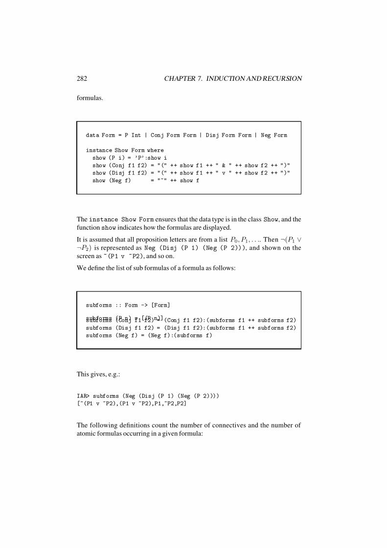
7/16/2019 The Haskell Road to Logic Maths and Programming
http://slidepdf.com/reader/full/the-haskell-road-to-logic-maths-and-programming-5634fa29ef7e9 293/448
282 CHAPTER 7. INDUCTION AND RECURSION
formulas.
data Form = P Int | Conj Form Form | Disj Form Form | Neg Form
instance Show Form where
show (P i) = ’P’:show i
show (Conj f1 f2) = "(" ++ show f1 ++ " & " ++ show f2 ++ ")"
show (Disj f1 f2) = "(" ++ show f1 ++ " v " ++ show f2 ++ ")"
show (Neg f) = "~" ++ show f
The instance Show Form ensures that the data type is in the class Show, and the
function show indicates how the formulas are displayed.
It is assumed that all proposition letters are from a list P 0, P 1, . . .. Then ¬(P 1 ∨¬P 2) is represented as Neg (Disj (P 1) (Neg (P 2))), and shown on the
screen as ~(P1 v ~P2), and so on.
We define the list of sub formulas of a formula as follows:
subforms :: Form -> [Form]
subforms (P n) = [(P n)]subforms (Conj f1 f2) = (Conj f1 f2):(subforms f1 ++ subforms f2)
subforms (Disj f1 f2) = (Disj f1 f2):(subforms f1 ++ subforms f2)
subforms (Neg f) = (Neg f):(subforms f)
This gives, e.g.:
IAR> subforms (Neg (Disj (P 1) (Neg (P 2))))
[~(P1 v ~P2),(P1 v ~P2),P1,~P2,P2]
The following definitions count the number of connectives and the number of
atomic formulas occurring in a given formula:

7/16/2019 The Haskell Road to Logic Maths and Programming
http://slidepdf.com/reader/full/the-haskell-road-to-logic-maths-and-programming-5634fa29ef7e9 294/448
7.7. INDUCTION AND RECURSION OVER OTHER DATA STRUCTURES283
ccount :: Form -> Intccount (P n) = 0
ccount (Conj f1 f2) = 1 + (ccount f1) + (ccount f2)
ccount (Disj f1 f2) = 1 + (ccount f1) + (ccount f2)
ccount (Neg f) = 1 + (ccount f)
acount :: Form -> Int
acount (P n) = 1
acount (Conj f1 f2) = (acount f1) + (acount f2)
acount (Disj f1 f2) = (acount f1) + (acount f2)acount (Neg f) = acount f
Now we can prove that the number of sub formulas of a formula equals the sum of
its connectives and its atoms:
Proposition 7.63 For every member f of Form:
length (subforms f) = (ccount f) + (acount f).
Proof.
Basis If f is an atom, then subforms f = [f], so this list has length 1. Also,
ccount f = 0 and acount f = 1.
Induction step If f is a conjunction or a disjunction, we have:
• length (subforms f) = 1 + (subforms f1) + (subforms f2),
• ccount f = 1 + (ccount f1) + (ccount f2),
• acount f = (acount f1) + (acount f2),
where f1 and f2 are the two conjuncts or disjuncts. By induction hypothe-
sis:
length (subforms f1) = (ccount f1) + (acount f1).
length (subforms f2) = (ccount f2) + (acount f2).

7/16/2019 The Haskell Road to Logic Maths and Programming
http://slidepdf.com/reader/full/the-haskell-road-to-logic-maths-and-programming-5634fa29ef7e9 295/448
284 CHAPTER 7. INDUCTION AND RECURSION
The required equality follows immediately from this.
If f is a negation, we have:
• length (subforms f) = 1 + (subforms f1),
• ccount f = 1 + (ccount f1),
• acount f = (acount f1),
and again the required equality follows immediately from this and the in-
duction hypothesis.
If one proves a property of formulas by induction on the structure of the formula,
then the fact is used that every formula can be mapped to a natural number thatindicates its constructive complexity: 0 for the atomic formulas, the maximum of
rank(Φ) and rank(Ψ) plus 1 for a conjunction Φ ∧ Ψ, and so on.
7.8 Further Reading
Induction and recursion are at the core of discrete mathematics. See [Bal91]. A
splendid textbook that teaches concrete (and very useful) mathematical skills in
this area is Graham, Knuth and Patashnik [GKP89]. Recursion is also crucial for
algorithm design. If you are specifically interested in the design and analysis of
algorithms you should definitely read Harel [Har87]. Algorithm design in Haskell
is the topic of [RL99].

7/16/2019 The Haskell Road to Logic Maths and Programming
http://slidepdf.com/reader/full/the-haskell-road-to-logic-maths-and-programming-5634fa29ef7e9 296/448
Chapter 8
Working with Numbers
Preview
When reasoning about mathematical objects we make certain assumptions about
the existence of things to reason about. In the course of this chapter we will take
a look at integers, rational numbers, real numbers, and complex numbers. We
will recall what they all look like, and we will demonstrate that reasoning about
mathematical objects can be put to the practical test by an implementation of the
definitions that we reason about. The implementations turn the definitions into
procedures for handling representations of the mathematical objects. This chapter
will also present some illuminating examples of the art of mathematical reasoning.
module WWN
where
import List
import Nats
285

7/16/2019 The Haskell Road to Logic Maths and Programming
http://slidepdf.com/reader/full/the-haskell-road-to-logic-maths-and-programming-5634fa29ef7e9 297/448
286 CHAPTER 8. WORKING WITH NUMBERS
8.1 A Module for Natural Numbers
The natural numbers are the conceptual basis of more involved number systems.
The implementation of Natural from the previous chapter has the advantage that
the unary representation makes the two cases for inductive proofs and recursive
definitions, Z and S n, very clear. We repeat the code of our implementation of
Natural, wrapped up this time in the form of a module, and integrated into the
Haskell type system: see Figure 8.1. Note that an implementation of quotRem
was added: quotRem n m returns a pair (q,r) consisting of a quotient and a
remainder of the process of dividing n by m, i.e., q and r satisfy 0 r < m and
q × m + r = n.
The integration of Natural in the system of Haskell types is achieved by means
of instance declarations. E.g., the declaration instance Ord Natural makes
the type Natural an instance of the class Ord. From an inspection of Prelude.hswe get that (i) a type in this class is assumed to also be in the class Eq , and (ii)
a minimal complete definition of a type in this class assumes definitions of <= or
compare. Condition (i) is fulfilled for Natural by the deriving Eq statement,
while (ii) is taken care of by the code for compare in the module. The general
code for class Ord provides methods for the relations <=, <, >=, >, and for the
comparison operators max and min, so putting Natural in class Ord provides us
with all of these.
Similarly, the declaration instance Enum Natural ensures that Natural is inthe class Enum. Definitions for the following functions for types in this class areprovided in the module:
succ :: Natural -> Naturalpred :: Natural -> Natural
toEnum :: Int -> Natural
fromEnum :: Natural -> Int
enumFrom :: Natural -> [Natural]
The general code for the class provides, e.g., enumFromTo, so we get:
Nats> enumFromTo Z (toEnum 5)
[Z,S Z,S (S Z),S (S (S Z)),S (S (S (S Z))),S (S (S (S (S Z))))]
Next, the declaration instance Num Natural ensures that Natural is in theclass Num. This is where the functions for addition, multiplication, sign, abso-
lute value belong, as well as a type conversion function fromInteger. Putting inthe appropriate definitions allows the use of the standard names for these opera-tors. In terms of these, Prelude.hs defines subtraction, the type conversion function
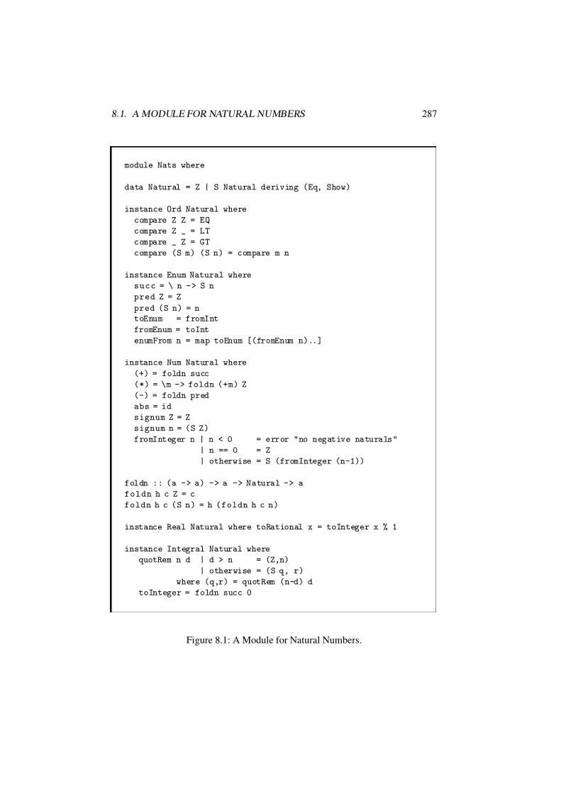
7/16/2019 The Haskell Road to Logic Maths and Programming
http://slidepdf.com/reader/full/the-haskell-road-to-logic-maths-and-programming-5634fa29ef7e9 298/448
8.1. A MODULE FOR NATURAL NUMBERS 287
module Nats where
data Natural = Z | S Natural deriving (Eq, Show)
instance Ord Natural where
compare Z Z = EQ
compare Z _ = LT
compare _ Z = GT
compare (S m) (S n) = compare m n
instance Enum Natural where
succ = \ n -> S n
pred Z = Z
pred (S n) = ntoEnum = fromInt
fromEnum = toInt
enumFrom n = map toEnum [(fromEnum n)..]
instance Num Natural where
(+) = foldn succ
(*) = \m -> foldn (+m) Z
(-) = foldn pred
abs = id
signum Z = Z
signum n = (S Z)
fromInteger n | n < 0 = error "no negative naturals"
| n == 0 = Z
| otherwise = S (fromInteger (n-1))
foldn :: (a -> a) -> a -> Natural -> a
foldn h c Z = c
foldn h c (S n) = h (foldn h c n)
instance Real Natural where toRational x = toInteger x % 1
instance Integral Natural where
quotRem n d | d > n = (Z,n)
| otherwise = (S q, r)
where (q,r) = quotRem (n-d) d
toInteger = foldn succ 0
Figure 8.1: A Module for Natural Numbers.

7/16/2019 The Haskell Road to Logic Maths and Programming
http://slidepdf.com/reader/full/the-haskell-road-to-logic-maths-and-programming-5634fa29ef7e9 299/448
288 CHAPTER 8. WORKING WITH NUMBERS
fromInt, and negate. Since negate is defined in terms of subtraction, and sub-
traction for naturals is cut-off subtraction, we get:
Nats> negate (S (S (S (S Z))))
Z
The next instance declaration puts Natural in the class Real. The only code
we have to provide is that for the type conversion function toRational. Putting
Natural in this class is necessary for the next move: the instance declaration
that puts Natural in the class Integral: types in this class are constrained by
Prelude.hs to be in the classes Real and Enum. The benefits of making Natural
an integral type are many: we now get implementations of even, odd, quot, rem,
div, mod, toInt and many other functions and operations for free (see the contents
of Prelude.hs for full details).
The implicit type conversion also allows us to introduce natural numbers in short-hand notation:
Nats> 12 :: Natural
S (S (S (S (S (S (S (S (S (S (S (S Z)))))))))))
The standard representation for natural numbers that we are accustomed to, deci-mal string notation, is built into the Haskell system for the display of integers. To
display naturals in decimal string notation, all we have to do is use type conversion:
Nats> toInt (S (S (S Z)))
3
Nats> (S (S Z)) ^ (S (S (S Z)))
S (S (S (S (S (S (S (S Z)))))))
Nats> toInt (S (S Z)) ^ (S (S (S Z)))
8
For other representations, i.e., binary string representation of an integral number
n, divide by 2 repeatedly, and collect the remainders in a list. The reversal of this
list gives the binary representation bk
. . . b0
satisfying n = bk ·
2k + bk−1 ·
2k−
1 +· · · + b0. The nice thing is that we can provide this code for the whole class of
Integral types:

7/16/2019 The Haskell Road to Logic Maths and Programming
http://slidepdf.com/reader/full/the-haskell-road-to-logic-maths-and-programming-5634fa29ef7e9 300/448
8.2. GCD AND THE FUNDAMENTAL THEOREM OF ARITHMETIC 289
binary :: Integral a => a -> [Int]binary x = reverse (bits x)
where bits 0 = [0]
bits 1 = [1]
bits n = toInt (rem n 2) : bits (quot n 2)
To display this on the screen, we need intToDigit for converting integers into
digital characters:
showDigits :: [Int] -> String
showDigits = map intToDigit
bin :: Integral a => a -> String
bin = showDigits . binary
Exercise 8.1 Give a function hex for displaying numbers in type class Integral
in hexadecimal form, i.e., in base 16 representation. The extra digits a, b, c, d,
e, f for 10, 11, 12, 13, 14, 15 that you need are provided by intToDigit. The
call hex 31 should yield "1f". (Hint: it is worthwhile to provide a more general
function toBase for converting to a list of digits in any base in
2, . . . , 16
, and
then define hex in terms of that.)
8.2 GCD and the Fundamental Theorem of Arith-
metic
The fundamental theorem of arithmetic, stating that every n ∈ N with n > 1 has
a unique prime factorization, was known in Antiquity. Let us reflect a bit to see
why it is true. First note that the restriction on n is necessary, for m · 0 = 0 for all
m ∈ N, so a factorization of 0 can never be unique, and since we have ruled out 1as a prime, 1 does not have a prime factorization at all. The fundamental theorem
of arithmetic constitutes the reason, by the way, for ruling out 1 as a prime number.
We have n = 1m · n for any n, m ∈ N, so a factorization of n that admits 1m as a
factor can never be unique.

7/16/2019 The Haskell Road to Logic Maths and Programming
http://slidepdf.com/reader/full/the-haskell-road-to-logic-maths-and-programming-5634fa29ef7e9 301/448
290 CHAPTER 8. WORKING WITH NUMBERS
From the prime factorization algorithm (1.7) we know that prime factorizations of
every natural number > 1 exist. To show uniqueness, we still have to establish thatno number has more than one prime factorization.
Euclid’s GCD algorithm The greatest common divisor of two natural numbers
a, b, notation GCD(a, b), is the natural number d with the property that d divides
both a and b, and for all natural numbers d that divide both a and b it holds that
d divides d. For example, GCD(30, 84) = 6, for 6 divides 30 and 84, and every
other common divisor of 30 and 84 divides 6 (these other common divisors being
1, 2 and 3).
Clearly, if such d exists, it is unique, for suppose that d also qualifies. Then
because d divides a and b, it follows from the definition of d that d divides d.
Similarly, because d divides a and b, it follows from the definition of d that ddivides d. But if d divides d and d divides d then it follows that d = d.
The greatest common divisor of a and b can be found from the prime factorizations
of a and b as follows. Let a = pα11 · · · pαkk and b = pβ11 · · · pβkk be prime factor-
izations of a and b, with p1, . . . , pk distinct primes, and α1, . . . , αk, β 1, . . . , β knatural numbers. Then the greatest common divisor of a and b equals the natural
number pγ 11 · · · pγ kk , where each γ i is the minimum of αi and β i.
For example, the greatest common divisor of 30 = 21 · 31 · 51 · 70 and 84 =22 · 31 · 50 · 71 is given by 21 · 31 · 50 · 70 = 6.
But there is an easier way to find GCD(a, b). Here is Euclid’s famous algorithm
(assume neither of a, b equals 0):
WHILE a = b DO IF a > b THEN a := a − b ELSE b := b − a.
Let us run this for the example case a = 30, b = 84. We get the following
(conventions about variable names as in Section 1.7).
a0 = 30 b0 = 84a0 < b0 a1 = 30 b1 = 84 − 30 = 54a1 < b1 a2 = 30 b2 = 54 − 30 = 24a2 > b2 a3 = 30 − 24 = 6 b3 = 24a3 < b3 a4 = 6 b4 = 24 − 6 = 18a4 < b4 a5 = 6 b5 = 18 − 6 = 12a5 < b5 a6 = 6 b6 = 12 − 6 = 6
a6 = b6 = 6
Now why does this work? The key observation is the following.

7/16/2019 The Haskell Road to Logic Maths and Programming
http://slidepdf.com/reader/full/the-haskell-road-to-logic-maths-and-programming-5634fa29ef7e9 302/448
8.2. GCD AND THE FUNDAMENTAL THEOREM OF ARITHMETIC 291
If d divides a and b and a > b then d divides a
−b (for then there are natural
numbers m, n with m > n and a = md , b = nd, and therefore a−b = md−nd =d(m − n)), and similarly, if d divides a and b and a < b then d divides b − a.
Conversely, if a > b and d divides a − b and b, then d divides a (for then there
are natural numbers m, n with a − b = md and b = nd, hence a = md + nd =d(m + n)), and similarly, if a > b and d divides b − a and a, then d divides a.
Thus, if a > b then the set of common divisors of a and b equals the set of common
divisors of a − b and b, and if b > a then the set of common divisors of a and bequals the set of common divisors of a and b − a.
Since the sets of all common divisors are equal, the greatest common divisors must
be equal as well. Therefore we have: if a > b then GCD(a, b) = GCD(a − b, b),
and if b > a then GCD(a, b) = GCD(a, b − a).
Using this we see that every iteration through the loop preserves the greatest com-mon divisor in the following sense: GCD(ai, bi) = GCD(ai+1, bi+1). Since we
know that the algorithm terminates we have: there is some k with ak = bk. There-
fore ak = GCD(ak, bk) = GCD(a, b).
Haskell contains a standard function gcd for the greatest common divisor of a pair
of objects of type Integral:
gcd :: Integral a => a -> a -> a
gcd 0 0 = error "Prelude.gcd: gcd 0 0 is undefined"
gcd x y = gcd’ (abs x) (abs y)
where gcd’ x 0 = xgcd’ x y = gcd’ y (x ‘rem‘ y)
Exercise 8.2 If you compare the code for gcd to Euclid’s algorithm, you see that
Euclid uses repeated subtraction where the Haskell code uses rem. Explain as
precisely as you can how the Haskell version of the GCD algorithm is related to
Euclid’s method for finding the GCD.
We can use the GCD to define an interesting relation. Two natural numbers n and
m are said to be co-prime or relatively prime if GCD(m, n) = 1. Here is an
implementation:

7/16/2019 The Haskell Road to Logic Maths and Programming
http://slidepdf.com/reader/full/the-haskell-road-to-logic-maths-and-programming-5634fa29ef7e9 303/448
292 CHAPTER 8. WORKING WITH NUMBERS
coprime :: Integer -> Integer -> Boolcoprime m n = (gcd m n) == 1
Exercise 8.3 Consider the following experiment:
WWN> coprime 12 25
True
WWN> 12 + 25
37
WWN> coprime 25 37
True
WWN> 25 + 3762
WWN> coprime 37 62
True
WWN> 37 + 62
99
WWN> coprime 62 99
True
WWN> 62 + 99
161
WWN> coprime 99 161
True
WWN>
This experiment suggests a general rule, for you to consider . . .
Does it follow from the fact that a and b are co-prime with a < b that b and a+b are
co-prime? Give a proof if your answer is ‘yes’ and a counterexample otherwise.
Theorem 8.4 For all positive a, b ∈ N there are integers m, n with ma + nb =GCD(a, b).
Proof. Consider the pairs (a0, b0), (a1, b1), . . . , (ak, bk) generated by Euclid’s
algorithm. We know that (a0, b0) = (a, b) and that ak = bk = GCD(a, b).
a0 satisfies a0 = ma + nb for m = 1, n = 0, b0 satisfies ma + nb = 1 for
m = 0, n = 1.
Suppose ai satisfies ai = m1a + n1b and bi satisfies bi = m2a + n2b. If ai > bi,then ai+1 satisfies ai+1 = (m1 − m2)a + (n1 − n2)b and bi+1 satisfies bi+1 =

7/16/2019 The Haskell Road to Logic Maths and Programming
http://slidepdf.com/reader/full/the-haskell-road-to-logic-maths-and-programming-5634fa29ef7e9 304/448
8.3. INTEGERS 293
m2a + n2b. If ai < bi, then ai+1 satisfies ai+1 = m1a + n1b and bi+1 satisfies
bi+1 = (m2−m1)a+(n2−n1)b. Thus, every iteration throughthe loop of Euclid’salgorithm preserves the fact that ai and bi are integral linear combinations ma+nbof a and b.
This shows that there are integers m, n with ak = ma + nb, hence that ma + nb =GCD(a, b).
Theorem 8.5 If p is a prime number that divides ab then p divides a or b.
Proof. Suppose p divides ab and p does not divide a. Then GCD(a, p) = 1. By
the previous theorem there are integers m, n with ma + np = 1. Multiplying both
sides by b gives:
mab + nbp = b.
By the fact that p divides ab we know that p divides both mab and nbp. Hence pdivides mab + nbp. Hence p divides b.
Theorem 8.5 is the tool for proving the fundamental theorem of arithmetic.
Theorem 8.6 (Fundamental Theorem of Arithmetic)
Every natural number greater than 1 has a unique prime factorization.
Proof. We established in 1.7 that every natural number greater than 1 has at least
one prime factorization.
To show that every natural number has at most one prime factorization, assume to
the contrary that there is a natural number N > 1 with at least two different primefactorizations. Thus,
N = p1 · · · pr = q 1 · · · q s,
with all of p1, . . . , pr, q 1, . . . , q s prime. Divide out common factors if necessary.
This gives a pi that is not among the q ’s. But this is a contradiction with theorem
8.5, because pi divides N = q 1 · · · q s but pi does not divide any of q 1, . . . , q s,
since these are all prime numbers different from pi.
8.3 Integers
Suppose n,m,k are natural numbers. When n = m + k we can view k as the
difference of n and m, and it is tempting to write this as k = n − m for the
operation of subtraction. Addition and subtraction are called inverse operations,

7/16/2019 The Haskell Road to Logic Maths and Programming
http://slidepdf.com/reader/full/the-haskell-road-to-logic-maths-and-programming-5634fa29ef7e9 305/448
294 CHAPTER 8. WORKING WITH NUMBERS
for if the addition of n to m is followed by the subtraction of n, the end result is
the original natural number m. In other words, we have:
(m + n) − n = m.
But we have to be careful here. The operation of subtracting a natural number nfrom a natural number m will only result in a natural number if m n. To make
subtraction possible between any pair of numbers, we have to introduce negative
numbers. This gives the domain of integers:
Z = . . . , −3, −2, −1, 0, 1, 2, 3, . . ..
The symbol Z derives from Zahl, the German word for number.
In fact, we need not consider the integers as given by God, but we can view them
as constructed from the natural numbers. This can be done in several ways. The
following Haskell code illustrates one possibility:
data Sgn = P | N deriving (Eq,Show)
type MyInt = (Sgn,Natural)
myplus :: MyInt -> MyInt -> MyInt
myplus (s1,m) (s2,n) | s1 == s2 = (s1,m+n)
| s1 == P && n <= m = (P,m-n)
| s1 == P && n > m = (N,n-m)
| otherwise = myplus (s2,n) (s1,m)
Another way is as follows. We represent every integer as a ‘difference pair’ of two
natural numbers. For example, (0, 3) represents −3, but the same number −3 is
also represented by (1, 4) or (2, 5).
In general, for all m1, m2 ∈ N, if m1 m2 then there is a k ∈ N with m2 + k =m1, and (m1, m2) represents k. If, on the other hand, m1 < m2 then there is a
k ∈ N with m1 + k = m2, and (m1, m2) represents −k. Thus, let R ⊆ N2 be
defined as follows:
(m1, m2)R(n1, n2) :≡ m1 + n2 = m2 + n1.
It is easy to see that R is an equivalence on N2. If m ∈ N, then the integer −m is
represented by (0, m), but also by (k, k + m), for any k
∈N.
Intuitively (m1, m2) and (n1, n2) are equivalent modulo R when their differences
are the same. This is the case precisely when m1 + n2 = m2 + n1. In this case we
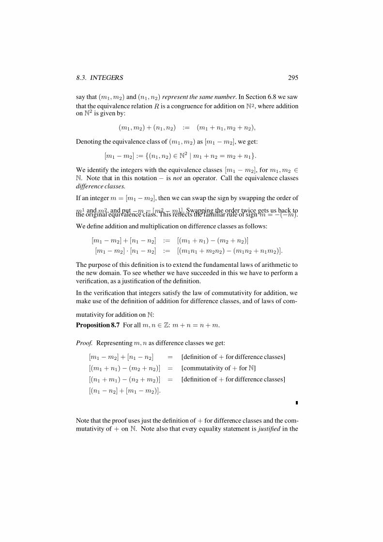
7/16/2019 The Haskell Road to Logic Maths and Programming
http://slidepdf.com/reader/full/the-haskell-road-to-logic-maths-and-programming-5634fa29ef7e9 306/448
8.3. INTEGERS 295
say that (m1, m2) and (n1, n2) represent the same number . In Section 6.8 we saw
that the equivalence relation R is a congruence for addition on N2, where additionon N2 is given by:
(m1, m2) + (n1, n2) := (m1 + n1, m2 + n2),
Denoting the equivalence class of (m1, m2) as [m1 − m2], we get:
[m1 − m2] := (n1, n2) ∈ N2 | m1 + n2 = m2 + n1.
We identify the integers with the equivalence classes [m1 − m2], for m1, m2 ∈N. Note that in this notation − is not an operator. Call the equivalence classes
difference classes.
If an integer m = [m1 − m2], then we can swap the sign by swapping the order of
m1 and m2, and put −m = [m2 − m1]. Swapping the order twice gets us back tothe original equivalence class. This reflects the familiar rule of sign m = −(−m).
We define addition and multiplication on difference classes as follows:
[m1 − m2] + [n1 − n2] := [(m1 + n1) − (m2 + n2)]
[m1 − m2] · [n1 − n2] := [(m1n1 + m2n2) − (m1n2 + n1m2)].
The purpose of this definition is to extend the fundamental laws of arithmetic to
the new domain. To see whether we have succeeded in this we have to perform a
verification, as a justification of the definition.
In the verification that integers satisfy the law of commutativity for addition, we
make use of the definition of addition for difference classes, and of laws of com-
mutativity for addition on N:
Proposition 8.7 For all m, n ∈ Z: m + n = n + m.
Proof. Representing m, n as difference classes we get:
[m1 − m2] + [n1 − n2] = [definition of + for difference classes]
[(m1 + n1) − (m2 + n2)] = [commutativity of + for N]
[(n1 + m1) − (n2 + m2)] = [definition of + for difference classes]
[(n1 − n2] + [m1 − m2)].
Note that the proof uses just the definition of + for difference classes and the com-
mutativity of + on N. Note also that every equality statement is justified in the

7/16/2019 The Haskell Road to Logic Maths and Programming
http://slidepdf.com/reader/full/the-haskell-road-to-logic-maths-and-programming-5634fa29ef7e9 307/448
296 CHAPTER 8. WORKING WITH NUMBERS
proof by a reference to a definition or to a fundamental law of arithmetic, where
these laws are in turn justified by inductive proofs based on the recursive defini-tions of the natural number operations. Thus, the fundamental laws of arithmetic
and the definition of a new kind of object (difference classes) in terms of a familiar
one (natural numbers) are our starting point for the investigation of that new kind
of object.
Exercise 8.8 Show (using the definition of integers as difference classes and the
definition of addition for difference classes) that the associative law for addition
holds for the domain of integers.
In a similar way it can be shown from the definition of integers by means of dif-ference classes and the definition of multiplication for difference classes that the
associative and commutative laws for multiplication continue to hold for the do-
main of integers.
As a further example of reasoning about this representation for the integers, we
show that the distributive law continues to hold in the domain of integers (viewed
as difference classes). In the verification we make use of the definition of addition
and multiplication for difference classes, and of the fundamental laws for addition
and multiplication on the natural numbers. Again, we justify every step by means
of a reference to the definition of an operation on difference classes or to one of
the laws of arithmetic for the natural numbers.
Proposition 8.9 For all m,n,k ∈ Z : m(n + k) = mn + mk.
Proof. Representing m,n,k as difference classes we get:
[m1 − m2]([n1 − n2] + [k1 − k2])
= [definition of + for difference classes]
[m1 − m2][(n1 + k1) − (n2 + k2)]
= [definition of · for difference classes]
[(m1(n1 + k1) + m2(n2 + k2)) − (m1(n2 + k2) + (n1 + k1)m2)]
= [distribution of · over + for N]
[(m1n1 + m1k1 + m2n2 + m2k2) − (m1n2 + m1k2 + m2n1 + m2k1)]

7/16/2019 The Haskell Road to Logic Maths and Programming
http://slidepdf.com/reader/full/the-haskell-road-to-logic-maths-and-programming-5634fa29ef7e9 308/448
8.4. IMPLEMENTING INTEGER ARITHMETIC 297
= [commutativity of + for N]
[(m1n1 + m2n2 + m1k1 + m2k2) − (m1n2 + m2n1 + m1k2 + m2k1)]
= [definition of + for difference classes]
[(m1n1 + m2n2) − (m1n2 + m2n1)]+ [(m1k1 + m2k2) − (m1k2 + m2k1)]
= [definition of · for difference classes]
[m1 − m2] · [n1 − n2] + [m1 − m2] · [k1 − k2].
Once the integers and the operations of addition and multiplication on it are de-
fined, and we have checked that the definitions are correct, we can forget of course
about the representation by means of difference classes. It simply takes too much
mental energy to keep such details of representation in mind. Mathematiciansmake friends with mathematical objects by forgetting about irrelevant details of
their definition.
The natural numbers have representations as difference classes too: a natural num-
ber m is represented by [m − 0]. In fact, the original numbers and their represen-
tations in the new domain Z behave exactly the same, in a very precise sense: the
function that maps m ∈ N to [m − 0] is one-to-one (it never maps different num-
bers to the same pair) and it preserves the structure of addition and multiplication,
in the following sense (see also Section 6.8). If m + n = k then
[m − 0] + [n − 0] = [(m + n) − 0] = [k − 0],
and if mn = k then
[m − 0] · [n − 0] = [mn − 0] = [k − 0].
Again we forget about the differences in representation and we say: N ⊆ Z.
8.4 Implementing Integer Arithmetic
If we represent natural numbers as type Natural, then the moral of the above is
that integers can be represented as pairs of naturals. E.g., minus five is represented
by the pair (S Z,S(S(S(S(S(S Z)))))), orby the pair (Z,S(S(S(S(S Z))))),
and so on. Here is an appropriate data type declaration:
type NatPair = (Natural,Natural)
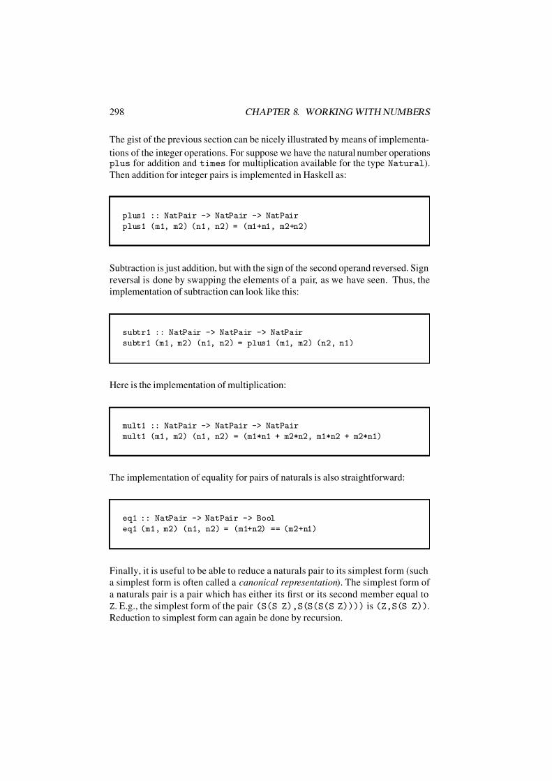
7/16/2019 The Haskell Road to Logic Maths and Programming
http://slidepdf.com/reader/full/the-haskell-road-to-logic-maths-and-programming-5634fa29ef7e9 309/448
298 CHAPTER 8. WORKING WITH NUMBERS
The gist of the previous section can be nicely illustrated by means of implementa-
tions of the integer operations. For suppose we have the natural number operationsplus for addition and times for multiplication available for the type Natural).
Then addition for integer pairs is implemented in Haskell as:
plus1 :: NatPair -> NatPair -> NatPair
plus1 (m1, m2) (n1, n2) = (m1+n1, m2+n2)
Subtraction is just addition, but with the sign of the second operand reversed. Sign
reversal is done by swapping the elements of a pair, as we have seen. Thus, the
implementation of subtraction can look like this:
subtr1 :: NatPair -> NatPair -> NatPair
subtr1 (m1, m2) (n1, n2) = plus1 (m1, m2) (n2, n1)
Here is the implementation of multiplication:
mult1 :: NatPair -> NatPair -> NatPair
mult1 (m1, m2) (n1, n2) = (m1*n1 + m2*n2, m1*n2 + m2*n1)
The implementation of equality for pairs of naturals is also straightforward:
eq1 :: NatPair -> NatPair -> Bool
eq1 (m1, m2) (n1, n2) = (m1+n2) == (m2+n1)
Finally, it is useful to be able to reduce a naturals pair to its simplest form (such
a simplest form is often called a canonical representation). The simplest form of
a naturals pair is a pair which has either its first or its second member equal to
Z. E.g., the simplest form of the pair (S(S Z),S(S(S(S Z)))) is (Z,S(S Z)).
Reduction to simplest form can again be done by recursion.

7/16/2019 The Haskell Road to Logic Maths and Programming
http://slidepdf.com/reader/full/the-haskell-road-to-logic-maths-and-programming-5634fa29ef7e9 310/448
8.5. RATIONAL NUMBERS 299
reduce1 :: NatPair -> NatPairreduce1 (m1,Z) = (m1,Z)
reduce1 (Z,m2) = (Z,m2)
reduce1 (S m1, S m2) = reduce1 (m1, m2)
Exercise 8.10 Define and implement relations leq1 for and gt1 for > for dif-
ference classes of naturals.
8.5 Rational Numbers
A further assumption that we would like to make is that any integer can be divided
by any non-zero integer to form a fraction, or rational number, and that any rational
number m/n can be ‘canceled down’ to its lowest form by dividing m and n by
the same number. E.g., 12/39 cancels down to 4/13.
Again we can view the rational numbers as constructed by means of pairs, in this
case pairs (m, n) with m, n ∈ Z, n = 0. In this case the pairs are ‘ratio pairs’.
One and the same rational number can be represented in many different ways:
(1, 2), (2, 4), (13, 26) all represent the rational number 1/2. Or in other words:
the rational number m/n is nothing but the class of all ( p, q ) with p, q ∈ Z, q = 0,
and the property that mq = np. In such a case we say that m/n and p/q represent
the same number.
As in the case of the representation of integers by means of difference classeswe have an underlying notion of equivalence. Let S be the equivalence relation on
Z×(Z−0) given by (m, n)S ( p, q ) :≡ mq = np. Note that (m, n) and (km,kn)are equivalent modulo S (provided k = 0), which justifies the simplification of
km/kn to m/n by means of canceling down. The set Q of rational numbers (or
fractional numbers) can be defined as:
Q := (Z× (Z− 0))/S.
We write a class [(m/n)]S as [m/n]. Addition, multiplication and equality of ra-
tional numbers are now defined in terms of addition and multiplication of integers,
as follows:
[m/n] + [ p/q ] := [(mq + pn)/nq ]
[m/n] · [ p/q ] := [mp/nq ]
[m/n] = [ p/q ] :≡ mq = np

7/16/2019 The Haskell Road to Logic Maths and Programming
http://slidepdf.com/reader/full/the-haskell-road-to-logic-maths-and-programming-5634fa29ef7e9 311/448
300 CHAPTER 8. WORKING WITH NUMBERS
Again, we have to check that these definitions make sense. It is easy to see that
the sum, the difference, and the product of two ratio classes are again ratio classes.For instance, if x ∈ Q and y ∈ Q, then there are integers m,n,p,q ∈ Z with
n = 0, q = 0, and x = [m/n] and y = [ p/q ]. Then x + y = [m/n] + [ p/q ] =[(mq + pn)/nq ], and from mq + pn ∈ Z, nq ∈ Z, and nq = 0 it follows that
x + y ∈ Q.
Proposition 8.11 The law of associativity for + holds for the rationals.
Proof. If x,y,z ∈ Q then there are m,n,p,q,r,s ∈ Zwith x = [m/n], y = [ p/q ],
z = [r/s], n = 0, q = 0 and s = 0 . Now:
x + (y + z)
= [definitions of x,y,z]
[mn
] + ([ pq
] + [ rs
])
= [definition of + for Q]
[mn ] + [ ps+rqqs ]
= [definition of + for Q]
[mqs+( ps+rq)n
nqs ]
= [distribution law for Z]
[mqs+ psn+rqnnqs
]
= [assoc of · for Z, dist law for Z]
[ (mq+ pn)s+rqnnqs ]
= [definition of + for Q]
[mq+ pnnq
] + [ rs
]
= [definition of + for Q]
([mn
] + [ pq
]) + [ rs
]
= [definitions of x,y,z]
(x + y) + z.
In a similar way, it is not difficult (but admittedly a bit tedious) to check that the
law of commutativity for + holds for the rationals, that the laws of associativity

7/16/2019 The Haskell Road to Logic Maths and Programming
http://slidepdf.com/reader/full/the-haskell-road-to-logic-maths-and-programming-5634fa29ef7e9 312/448
8.5. RATIONAL NUMBERS 301
and commutativity for
·hold for the rationals, and that the law of distribution holds
for the rationals.
A thing to note about Proposition 8.11 is that the statement about rational num-
bers that it makes also tells us something about our ways of doing things in an
implementation. It tells us that any program that uses the procedure add which
implements addition for the rationals need not distinguish between
(add (add (m,n) (p,q)) (r,s)) and (add (m,n) (add (p,q) (r,s))).
Wherever one expression fits the other will fit.
Again forgetting about irrelevant differences in representation, we see thatZ ⊆ Q,
for every integer n has a representation in the rationals, namely n/1.
If x, y∈Q, then x + y
∈Q, x
−y
∈Q, xy
∈Q. If, in addition y
= 0,
we have x/y ∈ Q. We say that the domain of rationals is closed under addition,
subtraction, and multiplication and ‘almost closed’ under division. If y = 0, then
1/y exists, which shows that every rational number y except 0 has an inverse: a
rational number that yields 1 when multiplied with y.
A domain of numbers that is closed under the four operations of addition, sub-
traction, multiplication and division (with the extra condition on division that the
divisor should be = 0) is called a field . The domain of rational numbers is a field.
It is easy to see that each rational number m/n can be written in decimal form, by
performing the process of long division. There are two possible outcomes:
1. the division process stops: m/n can be written as a finite decimal expansion.
2. the division process repeats: m/n can be written as a infinite decimal ex-pansion with a tail part consisting of a digit or group of digits which repeats
infinitely often.
Examples of the first outcome are 1/4 = 0.25, −1/4 = −0.25, 22/5 = 4.4.
Examples of the second outcome are 1/3 = 0.3333 . . ., 1/6 = 0.166666 . . .,29/7 = 4.142857142857142857 . . ., 23/14 = 1.6428571428571428571 . . .. A
handy notation for this is 1/3 = 0.3, 1/6 = 0.6, 29/7 = 4.142857, 23/14 =1.6428571. The part under the line is the part that repeats infinitely often.
If the division process repeats for m/n then at each stage of the process there must
be a non-zero remainder. This means that at each stage, the remainder must be in
the range 1, . . . , n − 1. But then after at most n steps, some remainder k is bound
to reoccur, and after the reappearance of k the process runs through exactly the
same stages as after the first appearance of k. The same remainders turn up, in the
same order. We are in a loop.

7/16/2019 The Haskell Road to Logic Maths and Programming
http://slidepdf.com/reader/full/the-haskell-road-to-logic-maths-and-programming-5634fa29ef7e9 313/448
302 CHAPTER 8. WORKING WITH NUMBERS
Conversely, it is not very difficult to see that every repeating decimal corresponds
to a rational number. First an example. Suppose M = 0.133133133 . . . = 0.133.Then: 1000 ∗ M = 133.133, and (1000 ∗ M ) − M = 133.133 − 0.133 = 133, so
M = 133999 .
Now for the general case.
Theorem 8.12 Every repeating decimal corresponds to a rational number.
Proof. A repeating decimal can always be written in our over-line notation in the
form
M ± 0.a1a2 · · · amb1b2 · · · bn,
where M is an integer and the ai and bj are decimal digits. For example,
−37/14 =
−2.6428571 = −2 − 0.6428571. If we can prove that the part
p = 0.a1a2 · · · amb1b2 · · · bn
is rational, then we are done, for if p is rational and M is an integer then there
are integers n, k with p = n/k, so M + p = M + n/k = kM +nk
, i.e., M + p is
rational, and similarly for M − p. Setting
A = 0.a1a2 · · · am, B = 0.b1b2 · · · bn, C = 0.b1b2 · · · bn,
we get
p = 0.a1a2 · · · amb1b2 · · · bn = A + 10−mC.
If we can write this in terms of rational operations on A and B we are done.
C = 0.b1b2 · · · bn = 0.b1b2 · · · bnb1b2 · · · bn.
Thus,
C − 10−nC = 0.b1b2 · · · bnb1b2 · · · bn − 0.01 · · · 0nb1b2 · · · bn =
= 0.b1b2 · · · bn = B.
Therefore, C = B1−10−n , and we get:
p = A +10−mB
1 − 10−n,
so we have proved that p is rational.

7/16/2019 The Haskell Road to Logic Maths and Programming
http://slidepdf.com/reader/full/the-haskell-road-to-logic-maths-and-programming-5634fa29ef7e9 314/448
8.5. RATIONAL NUMBERS 303
r1
r3
r
2
t t t t t t t t t
t t t r
23
Figure 8.2: Constructing the fraction 2/3.
There is a nice geometrical interpretation of the process of constructing rational
numbers. Assume that we have been given the line of integers:
. . .−3• −2• −1• 0• 1• 2• 3• . . .
Place these on a (horizontal) x-axis and a (vertical) y-axis:
...
••
x · · · • • • • • · · ·•
•...y
Now construct further points on the x-axis by first drawing a straight line l through
a point m on the x-axis and a point n on the y-axis, and next drawing a line l
parallel to l through the point (0, 1). The intersection of l and the x-axis is the
rational point m/n. (Use congruence reasoning for triangles to establish that the
ratio between m and n equals the ratio between the intersection point m/n and 1.)
Figure 8.2 gives the construction of the fraction 2/3 on the x-axis.
Figures 8.3, 8.4, 8.5 and 8.6 give the geometrical interpretations of addition, nega-
tion, multiplication and reciprocal. Subtraction is addition of a negated number,
division is multiplication with a reciprocal, so these give all the rational operations.
Note that these constructions can all be performed by a process of (i) connecting
previously constructed points by a straight line, and (ii) drawing lines parallel to

7/16/2019 The Haskell Road to Logic Maths and Programming
http://slidepdf.com/reader/full/the-haskell-road-to-logic-maths-and-programming-5634fa29ef7e9 315/448
304 CHAPTER 8. WORKING WITH NUMBERS
0 1 a b a + b
1
a
Figure 8.3: Geometrical Interpretation of Addition.
0 1−1 a
a
−a
Figure 8.4: Geometrical Interpretation of Negation.
0 1 a b ab
1
1b
Figure 8.5: Geometrical Interpretation of Multiplication.

7/16/2019 The Haskell Road to Logic Maths and Programming
http://slidepdf.com/reader/full/the-haskell-road-to-logic-maths-and-programming-5634fa29ef7e9 316/448
8.6. IMPLEMENTING RATIONAL ARITHMETIC 305
1a
0 1 a
1
a
Figure 8.6: Geometrical Interpretation of Reciprocal.
previously constructed lines. These are the so-called linear constructions: the con-
structions that can be performed by using a ruler but no compass. In particular, use
of a compass to construct line segments of equal lengths is forbidden.
8.6 Implementing Rational Arithmetic
Haskell has a standard implementation of the above, a type Rational, predefined
as follows:
data Integral a => Ratio a = a :% a deriving (Eq)
type Rational = Ratio Integer
To reduce a fraction to its simplest form, we first make sure that the denominatoris non-negative. If (x,y) represents a fraction with numerator x and denominatory, then
(x * signum y) (abs y)
is an equivalent representation with positive denominator. Here abs gives the ab-
solute value, and signum the sign (1 for positive integers, 0 for 0, −1 for negative
integers). The reduction to canonical form is performed by:
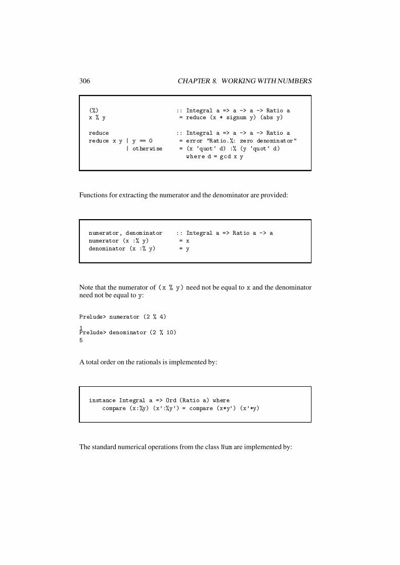
7/16/2019 The Haskell Road to Logic Maths and Programming
http://slidepdf.com/reader/full/the-haskell-road-to-logic-maths-and-programming-5634fa29ef7e9 317/448
306 CHAPTER 8. WORKING WITH NUMBERS
(%) :: Integral a => a -> a -> Ratio ax % y = reduce (x * signum y) (abs y)
reduce :: Integral a => a -> a -> Ratio a
reduce x y | y == 0 = error "Ratio.%: zero denominator"
| otherwise = (x ‘quot‘ d) :% (y ‘quot‘ d)
where d = gcd x y
Functions for extracting the numerator and the denominator are provided:
numerator, denominator :: Integral a => Ratio a -> a
numerator (x :% y) = x
denominator (x :% y) = y
Note that the numerator of (x % y) need not be equal to x and the denominatorneed not be equal to y:
Prelude> numerator (2 % 4)
1Prelude> denominator (2 % 10)
5
A total order on the rationals is implemented by:
instance Integral a => Ord (Ratio a) where
compare (x:%y) (x’:%y’) = compare (x*y’) (x’*y)
The standard numerical operations from the class Num are implemented by:

7/16/2019 The Haskell Road to Logic Maths and Programming
http://slidepdf.com/reader/full/the-haskell-road-to-logic-maths-and-programming-5634fa29ef7e9 318/448
8.6. IMPLEMENTING RATIONAL ARITHMETIC 307
instance Integral a => Num (Ratio a) where(x:%y) + (x’:%y’) = reduce (x*y’ + x’*y) (y*y’)
(x:%y) * (x’:%y’) = reduce (x*x’) (y*y’)
negate (x :% y) = negate x :% y
abs (x :% y) = abs x :% y
signum (x :% y) = signum x :% 1
The rationals are also closed under the division operation λxy.xy
and the reciprocal
operation λx. 1x . These are implemented as follows:
instance Integral a => Fractional (Ratio a) where(x:%y) / (x’:%y’) = (x*y’) % (y*x’)
recip (x:%y) = if x < 0 then (-y) :% (-x) else y :% x
If you want to try out decimal expansions of fractions on a computer, here is a
Haskell program that generates the decimal expansion of a fraction.
decExpand :: Rational -> [Integer]
decExpand x | x < 0 = error "negative argument"
| r == 0 = [q]
| otherwise = q : decExpand ((r*10) % d)where
(q,r) = quotRem n d
n = numerator x
d = denominator x
If the decimal expansion repeats, you will have to interrupt the process by typingcontrol c:
WWN> decExpand (1 % 7)
[0, 1, 4, 2, 8, 5, 7, 1, 4, 2, 8, 5, 7, 1, 4, 2, 8, 5, 7, 1, 4, 2, 8,
5, 7, 1, 4, 2, 8, 5, 7, 1, 4, 2, 8, 5, 7, 1, 4, 2, 8, 5, 7, 1, 4, 2,
8, 5, 7, 1, 4, 2, 8, 5, 7, 1, 4, 2, 8, 5, 7, 1, 4, 2, 8, 5, 7, 1, 4,2, 8, 5, 7, 1, 4, 2, 8, 5, 7, 1, 4, 2, 8, 5, 7, 1, 4, 2, 8, 5, 7, 1,
4, 2, 8, 5,Interrupted!

7/16/2019 The Haskell Road to Logic Maths and Programming
http://slidepdf.com/reader/full/the-haskell-road-to-logic-maths-and-programming-5634fa29ef7e9 319/448
308 CHAPTER 8. WORKING WITH NUMBERS
This problem can be remedied by checking every new quotient remainder pair
against a list of quotient-remainder pairs, to spot a repetition. The main functiondecForm produces the integer part, and relegates the task of calculating the lists of
non-repeating and repeating decimals to an auxiliary function decF.
decForm :: Rational -> (Integer,[Int],[Int])
decForm x | x < 0 = error "negative argument"
| otherwise = (q,ys,zs)
where
(q,r) = quotRem n d
n = numerator x
d = denominator x
(ys,zs) = decF (r*10) d []
The function decF has a parameter for the list of quotient remainder pairs that
have to be checked for repetition. The code for dForm uses elemIndex from the
module List.hs to find the index of the first repeating digit, and splitAt to split
a list at an index.
decF :: Integer -> Integer -> [(Int,Integer)] -> ([Int],[Int])
decF n d xs | r == 0 = (reverse (q: (map fst xs)),[])
| elem (q,r) xs = (ys,zs)
| otherwise = decF (r*10) d ((q,r):xs)
where(q’,r) = quotRem n d
q = toInt q’
xs’ = reverse xs
Just k = elemIndex (q,r) xs’
(ys,zs) = splitAt k (map fst xs’)
Here are a few examples:
WWN> decForm (133 % 999)
(0,[],[1,3,3])
WWN> decForm (1 % 7)(0,[],[1,4,2,8,5,7])
WWN> decForm (2 % 7)

7/16/2019 The Haskell Road to Logic Maths and Programming
http://slidepdf.com/reader/full/the-haskell-road-to-logic-maths-and-programming-5634fa29ef7e9 320/448
8.7. IRRATIONAL NUMBERS 309
(0,[],[2,8,5,7,1,4])
WWN> decForm (3 % 7)(0,[],[4,2,8,5,7,1])
WWN> decForm (4 % 7)
(0,[],[5,7,1,4,2,8])
WWN> decForm (5 % 7)
(0,[],[7,1,4,2,8,5])
WWN> decForm (6 % 7)
(0,[],[8,5,7,1,4,2])
There is no upper limit to the length of the period. Here is an example with a
period length of 99:
WWN> decForm (468 % 199)
(2,[],[3,5,1,7,5,8,7,9,3,9,6,9,8,4,9,2,4,6,2,3,1,1,5,5,7,7,8,8,9,4,4,7,2,3,6,1,8,0,9,0,4,5,2,2,6,1,3,0,6,5,3,2,6,6,3,3,1,6,5,8,2,9,1,4,5,
7,2,8,6,4,3,2,1,6,0,8,0,4,0,2,0,1,0,0,5,0,2,5,1,2,5,6,2,8,1,4,0,7,0])
Exercise 8.13 Write a Haskell program to find the longest period that occurs in
decimal expansions of fractions with numerator and denominator taken from the
set 1, . . . , 999.
8.7 Irrational Numbers
The Ancients discovered to their dismay that with just ruler and compass it is
possible to construct line segments whose lengths do not form rational fractions.
In other words, it is possible to construct a length q such that for no m, n ∈ Nit holds that q = m
n . Here is the famous theorem from Antiquity stating this
disturbing fact, with its proof.
1
1
d d d d d d d d d
x

7/16/2019 The Haskell Road to Logic Maths and Programming
http://slidepdf.com/reader/full/the-haskell-road-to-logic-maths-and-programming-5634fa29ef7e9 321/448
310 CHAPTER 8. WORKING WITH NUMBERS
Theorem 8.14 There is no rational number x with x2 = 2.
Proof. Assume there is a number x ∈ Q with x2 = 2. Then there are m, n ∈ Z,
n = 0 with (m/n)2 = 2. We can further assume that m/n is canceled down to its
lowest form, i.e., there are no k,p,q ∈ Z with k = 1, m = kp and n = kq .
We have: 2 = (m/n)2 = m2/n2, and multiplying both sides by n2 we find
2n2 = m2. In other words, m2 is even, and since squares of odd numbers are
always odd, m must be even, i.e., there is a p with m = 2 p. Substitution in
2n2 = m2 gives 2n2 = (2 p)2 = 4 p2, and we find that n2 = 2 p2, which leads to
the conclusion that n is also even. But this means that there is a q with n = 2q ,and we have a contradiction with the assumption that m/n was in lowest form. It
follows that there is no number x ∈ Q with x2 = 2. The square root of 2 is not
rational.
Of course, we all use√
2 for the square root of 2. The theorem tells us that√
2 /∈Q. The collection of numbers that
√ 2 does belong to is called the collection of
real numbers, R. It is possible to give a formal construction of the reals from the
rationals, but we will not do so here. Instead, we just mention that Q ⊆ R, and
we informally introduce the reals as the set of all signed (finite or infinite) decimal
expansions. The domain of real numbers is closed under the four operations of
addition, subtraction, multiplication and division, i.e., just like the rationals, the
reals form a field .
Exercise 8.15 Use the method from the proof of Theorem 8.14 to show that√
3is irrational.
Exercise 8.16 Show that if p is prime, then√
p is irrational.
Exercise 8.17 Show that if n is a natural number with√
n not a natural number,
then√
n is irrational.
Using the fundamental theorem of arithmetic, we can give the following alternative
proof of Theorem 8.14:
Proof. If √
2 = ( p/q ), then 2q 2 = p2. In the representation of p2 as a product
of prime factors, every prime factor has an even number of occurrences (for the
square of p equals the product of the squares of p’s prime factors). In the represen-
tation of 2q 2 as a product of prime factors, the prime factor 2 has an odd number
of occurrences. Contradiction with Theorem 8.6.

7/16/2019 The Haskell Road to Logic Maths and Programming
http://slidepdf.com/reader/full/the-haskell-road-to-logic-maths-and-programming-5634fa29ef7e9 322/448
8.7. IRRATIONAL NUMBERS 311
In Section 8.8 we will discuss an algorithm, the mechanic’s rule, for approaching
the square root of any positive fraction p with arbitrary precision.
The irrational numbers are defined here informally as the infinite non-periodic
decimal expansions. This is not a very neat definition, for its relies on the use of
decimals, and there is nothing special about using the number ten as a basis for
doing calculations. Other bases would serve just as well. In any case, looking at Q
and R in terms of expansions provides a neat perspective on the relation between
rational and irrational numbers. What, e.g., are the odds against constructing a
rational by means of a process of tossing coins to get an infinite binary expansion?
Exercise 8.18 Does it follow from the fact that x + y is rational that x is rational
or y is rational? If so, give a proof, if not, give a refutation.
We have seen that writing out the decimal expansion of a real number like √ 2 doesnot give a finite representation. In fact, since there are uncountably many reals (see
Chapter 11), no finite representation scheme for arbitrary reals is possible.
In implementations it is customary to use floating point representation (or: scien-tific representation) of approximations of reals. E.g., the decimal fraction 1424213.56is an approximation of
√ 2 × 10⁶, and gets represented as 1.42421356E + 5. The
decimal fraction 0.00000142421356 is an approximation of √
2106 =
√ 2 × 10⁻⁶,
and gets represented as 1.42421356E − 6. The general form is x.xxxEm, wherex.xxx is a decimal fraction called the mantissa and m is an integer called theexponent . Here are the Hugs versions:
Prelude> sqrt 2 * 10 6
1.41421e+06
Prelude> sqrt 2 / 10 61.41421e-06
Haskell has a predefined type Float for single precision floating point numbers,and a type Double for double precision floating point numbers. Together thesetwo types form the class Floating:
Prelude> :t sqrt 2
sqrt 2 :: Floating a => a
Floating point numbers are stored as pairs (m, n), where m is the matrix and nthe exponent of the base used for the encoding. If x is a floating point number, thebase of its representation is given by floatRadix and its matrix and exponent, as a
value of type (Integer,Int), by decodeFloat. Thus, if floatRadix x equalsb and decodeFloat x equals (m, n), then x is the number m · bn. floatDigitsgives the number of digits of m in base b representation. In particular, if (m, n)

7/16/2019 The Haskell Road to Logic Maths and Programming
http://slidepdf.com/reader/full/the-haskell-road-to-logic-maths-and-programming-5634fa29ef7e9 323/448
312 CHAPTER 8. WORKING WITH NUMBERS
is the value of decodeFloat x, and d the value of floatDigits, then either m
and n are both zero, or bd−1 m < bd. Here is an example:
Prelude> floatRadix (sqrt 2)
2
Prelude> decodeFloat (sqrt 2)
(11863283,-23)
Prelude> 11863283 * 2^^(-23)
1.41421
Prelude> floatDigits (sqrt 2)
24
Prelude> 2^23 <= 11863283 && 11863283 < 2^24
True
The inverse to the function decodeFloat is encodeFloat:
Prelude> sqrt 2
1.41421
Prelude> encodeFloat 11863283 (-23)
1.41421
Scaling a floating point number is done by ‘moving the point’:
Prelude> scaleFloat 4 (sqrt 2)
22.6274
Prelude> 2^4 * sqrt 2
22.6274
A floating point number can always be scaled in such a way that its matrix is inthe interval (−1, 1). The matrix in this representation is given by the functionsignificand, the exponent by exponent:
Prelude> significand (sqrt 2)
0.707107
Prelude> exponent (sqrt 2)
1
Prelude> 0.707107 * 2^1
1.41421
Prelude> scaleFloat 1 0.707107
1.41421
The definitions of exponent, significand and scaleFloat (from the Prelude):

7/16/2019 The Haskell Road to Logic Maths and Programming
http://slidepdf.com/reader/full/the-haskell-road-to-logic-maths-and-programming-5634fa29ef7e9 324/448
8.8. THE MECHANIC’S RULE 313
exponent x = if m==0 then 0 else n + floatDigits xwhere (m,n) = decodeFloat x
significand x = encodeFloat m (- floatDigits x)
where (m,_) = decodeFloat x
scaleFloat k x = encodeFloat m (n+k)
where (m,n) = decodeFloat x
8.8 The Mechanic’s Rule
Sequences of fractions can be used to find approximations to real numbers that
themselves are not fractions (see Section 8.7). A well known algorithm for gen-
erating such sequences is the so-called mechanic’s rule (also known as Newton’s
method , a bit misleadingly, for the algorithm was already in use centuries before
Newton):
p > 0, a0 > 0, an+1 =1
2(an +
p
an).
In Exercise 8.19 you are asked to prove that this can be used to approximate the
square root of any positive fraction p to any degree of accuracy. The Haskell im-
plementation uses some fresh ingredients. The function recip takes the reciprocal
of a fraction, the operation iterate iterates a function by applying it again to the
result of the previous application, and takeWhile takes a property and a list andconstructs the largest prefix of the list consisting of objects satisfying the property.
In the present case, the property is (\ m -> m^2 <= p), having a square p,
and the list is the list of positive naturals. You should look up the implementations
in Prelude.hs and make sure you understand.
mechanicsRule :: Rational -> Rational -> Rational
mechanicsRule p x = (1 % 2) * (x + (p * (recip x)))
mechanics :: Rational -> Rational -> [Rational]
mechanics p x = iterate (mechanicsRule p) x

7/16/2019 The Haskell Road to Logic Maths and Programming
http://slidepdf.com/reader/full/the-haskell-road-to-logic-maths-and-programming-5634fa29ef7e9 325/448
314 CHAPTER 8. WORKING WITH NUMBERS
sqrtM :: Rational -> [Rational]sqrtM p | p < 0 = error "negative argument"
| otherwise = mechanics p s
where
s = if xs == [] then 1 else last xs
xs = takeWhile (\ m -> m^2 <= p) [1..]
As a demonstration, here are the first seven steps in the approximation to√
2, the
first seven steps in the approximation to√
4, and the first, second, . . . , sixth step in
the approximation to√
50, respectively. This already gives greater accuracy thanis needed in most applications; the algorithm converges very fast.
WWN> take 5 (sqrtM 2)
[1 % 1,3 % 2,17 % 12,577 % 408,665857 % 470832]
WWN> take 7 (sqrtM 4)
[2 % 1,2 % 1,2 % 1,2 % 1,2 % 1,2 % 1,2 % 1]
WWN> sqrtM 50 !! 0
7 % 1
WWN> sqrtM 50 !! 1
99 % 14
WWN> sqrtM 50 !! 2
19601 % 2772
WWN> sqrtM 50 !! 3
768398401 % 108667944
WWN> sqrtM 50 !! 4
1180872205318713601 % 167000548819115088
Exercise 8.19 1. Prove that for every n,
an+1 − √ p
an+1 +√
p=
(an − √ p)2
(an +√
p)2.
2. From the first item it follows (by induction on n) that
an+1 − √ p
an+1 +√
p=
a0 − √
p
a0 +√
p
2n
.
Derive from this that sqrtM p converges to √ p for any positive rational
number p.
7/16/2019 The Haskell Road to Logic Maths and Programming
http://slidepdf.com/reader/full/the-haskell-road-to-logic-maths-and-programming-5634fa29ef7e9 326/448
8.9. REASONING ABOUT REALS 315
3. Show that the approximation is from above, i.e., show that n 1 implies
that an √ p.
Exercise 8.20 1. Find a rule to estimate the number of correct decimal places
in approximation an of √
p. Use the result of Exercise 8.19. (Hint: try
to find an inequality of the form an − √ p t, with t an expression that
employs a0 and a1.)
2. Use the previous item to give an estimate of the number of correct decimal
places in the successive approximations to√
2.
8.9 Reasoning about Reals
Suppose one wants to describe the behaviour of moving objects by plotting their
position or speed as a function of time. Moving objects do not suddenly disappear
and reappear somewhere else (outside the Bermuda triangle, at least), so the path
of a moving object does not have holes or gaps in it. This is where the notions of
continuity and limit arise naturally. Analysis, with its emphasis on continuity and
limit, is a rich source of examples where skill in quantifier reasoning is called for.
The following Lemma illustrates that many common functions are continuous. Its
proof is given as an example: it is a nice illustration of the use of the logical rules.
In fact, logic is all there is to this proof: properties of real numbers are not needed
at all.
Lemma. The composition of two continuous functions is continuous.
I.e., if f and g are continuous functions from reals to reals, then the function hdefined by h(x) = g(f (x)) (cf. Definition 6.29 p. 222) is continuous as well.
Proof. Given: f and g are continuous, i.e., (“ε-δ -definition” p. 66; for clarity we
use different variables for the arguments):
∀x ∀ε > 0 ∃δ > 0 ∀y (|x − y| < δ =⇒ |f (x) − f (y)| < ε), (8.1)
∀a ∀ε > 0 ∃δ > 0 ∀b (|a − b| < δ =⇒ |g(a) − g(b)| < ε). (8.2)
To be proved: ∀x ∀ε > 0 ∃δ > 0 ∀y (|x − y| < δ =⇒ |g(f (x)) − g(f (y))| < ε).

7/16/2019 The Haskell Road to Logic Maths and Programming
http://slidepdf.com/reader/full/the-haskell-road-to-logic-maths-and-programming-5634fa29ef7e9 327/448
316 CHAPTER 8. WORKING WITH NUMBERS
Proof (detailed version): Note that what is To be proved begins with two universal
quantifiers ∀x and ∀ε > 0. Therefore, the proof has to start (recall the obligatoryopening that goes with ∀-introduction!) with choosing two arbitrary values x ∈ Rand ε > 0. We now have to show that
∃δ > 0 ∀y (|x − y| < δ =⇒ |g(f (x)) − g(f (y))| < ε). (8.3)
The next quantifier asks us to supply some example-δ that is > 0. There appears
to be no immediate way to reduce the proof problem further, so we start looking at
the givens in order to obtain such an example.
It turns out that we have to use the second given (8.2) first . It can be used (∀-
elimination) if we specify values for a and ε. Later on it will show that a = f (x)and the earlier ε will turn out to be useful.
Thus, (8.2) delivers (∃-elimination) some δ 1 > 0 such that
∀b (|f (x) − b| < δ 1 =⇒ |g(f (x)) − g(b)| < ε). (8.4)
Applying the given (8.1) to our x and ε = δ 1 (∀-elimination) we obtain (∃-
elimination) δ > 0 such that
∀y (|x − y| < δ =⇒ |f (x) − f (y)| < δ 1). (8.5)
And this is the example-δ we are looking for, i.e.:
Claim: ∀y (|x − y| < δ =⇒ |g(f (x)) − g(f (y))| < ε).
(From this follows what we have to show using
∃-introduction.)
Proof: Suppose that (to prepare for ∀-introduction and Deduction Rule — cf. Ex-
ercise 3.18 p. 93) y is such that |x − y| < δ .
From (8.5) (using this y — ∀-elimination and Modus Ponens) you find, that |f (x)−f (y)| < δ 1.
Finally, from (8.4) (with b = f (y) — ∀-elimination) you find that |g(f (x)) −g(f (y))| < ε.
The Claim follows.
Making up the score: the proof applies one rule for each of the fifteen (!) occur-
rences of logical symbols in Given and To be proved. Make sure you understand
every detail.
Of course, the amount of detail is excessive and there is a more common concise
version as well. The following version is the kind of argument you will find in

7/16/2019 The Haskell Road to Logic Maths and Programming
http://slidepdf.com/reader/full/the-haskell-road-to-logic-maths-and-programming-5634fa29ef7e9 328/448
8.9. REASONING ABOUT REALS 317
analysis textbooks. As is usual, it leaves to the reader to fill in which rules have
been applied, and where.
Proof. Assume that x ∈ R and ε > 0.
From (8.2), obtain δ 1 > 0 such that
∀b (|f (x) − b| < δ 1 =⇒ |g(f (x)) − g(b)| < ε). (8.6)
Applying (8.1) to x and δ 1, obtain δ > 0 such that
∀y (|x − y| < δ =⇒ |f (x) − f (y)| < δ 1). (8.7)
Then if
|x
−y
|< δ , by (8.7) we get that
|f (x)
−f (y)
|< δ 1, and from (8.6) it
follows that |g(f (x)) − g(f (y))| < ε.
This version of the proof will be considered very complete by every mathemati-
cian. Nevertheless, the compression attained is approximately 4 : 1.
The remaining examples of this section are about sequences of reals.
Limits. Assume that a0, a1, a2, . . . is a sequence of reals and that a ∈ R. The
expression limi→∞ ai = a (“the sequence converges to a”, “a is limit of the se-
quence”) by definition means that
∀ε > 0 ∃n ∀i n (|a − ai| < ε).
Generating concrete examples of converging sequences in Haskell is easy, as wehave seen in Section 8.8. We have seen that the sequences produced by the me-
chanic’s rule converge. We will prove some results about convergence.
Theorem. Every sequence of reals has at most one limit.
Proof. The situation should be analyzed as follows.
Given: limi→∞ ai = a, limi→∞ ai = b.
To be proved: a = b.
Proof: Proof by Contradiction is not a bad idea here, since the new given it pro-
vides, nl., that a = b, is equivalent with the positive |a − b| > 0. Thus, assume
this. Proof by Contradiction now asks to look for something false.
In order to use the old given, you need to choose (∀-elimination!) values for ε. As
you’ll see later, it is useful to choose ε = 12|a − b|. Note that ε > 0.
7/16/2019 The Haskell Road to Logic Maths and Programming
http://slidepdf.com/reader/full/the-haskell-road-to-logic-maths-and-programming-5634fa29ef7e9 329/448
318 CHAPTER 8. WORKING WITH NUMBERS
From the given limi
→∞ai = a we obtain now, that
∃n
∀i n (
|a
−ai
|< ε).
Thus (∃-elimination) some n1 exists such that ∀i n1 (|a − ai| < ε).
From the given limi→∞ ai = b we obtain, similarly, some n2 such that ∀i n2(|b − ai| < ε).
Define n = max(n1, n2). Since n n1, n2, by ∀-elimination we now get from
these facts that both |a − an| < ε and |b − an| < ε.
Lastly, using the triangle-inequality
|x + y| |x| + |y|,
it follows that |a − b| = |a − an + an − b| |a − an| + |b − an| < 2ε = |a − b|— and this is the falsity looked for.
Exercise 8.21 Write a concise version of the above proof.
Exercise 8.22 Assume that limi→∞ ai = a.
1. Show that limi→∞ a2i = a.
2. Assume that f : N → N is a function such that ∀n∃m∀i m f (i) n.
Show that limi→∞ af (i) = a.
Exercise 8.23 Assume that the sequences of reals
an
∞n=0 and
bn
∞n=0 have
limits a resp. b, and that a < b. Show that a number n exists such that ∀m n (am < bm).
Exercise 8.24 Assume that limi→∞ ai = a and that limi→∞ bi = b.
Show that limi→∞(ai + bi) = a + b.
Exercise 8.25 Show that a function f : R → R is continuous iff limi→∞ f (ai) =f (a) whenever limi→∞ ai = a.
Cauchy. A sequence of reals
an
∞n=0
is called Cauchy if
∀ε > 0 ∃n ∀i, j n (|ai − aj| < ε).

7/16/2019 The Haskell Road to Logic Maths and Programming
http://slidepdf.com/reader/full/the-haskell-road-to-logic-maths-and-programming-5634fa29ef7e9 330/448
8.10. COMPLEX NUMBERS 319
Exercise 8.26 Assume that the sequence
an
∞n=0 is Cauchy.
1. Show that the sequence is bounded . I.e., that numbers b and c exist such that
∀i (b < ai < c).
2. Assume that a ∈ R is such that ∀ε > 0∀n∃i n (|a − ai| < ε). (The
existence of such an a follows from the sequence being bounded, but you
are not asked to prove this.) Show that limi→∞ ai = a.
It follows immediately from Exercise 8.19 that the sequences of rationals produced
by the Mechanic’s rule are Cauchy. Thanks to that we can implement a program
for calculating square roots as follows (for still greater precision, change the value
of ε in apprx):
approximate :: Rational -> [Rational] -> Rational
approximate eps (x:y:zs)
| abs (y-x) < eps = y
| otherwise = approximate eps (y:zs)
apprx :: [Rational] -> Rational
apprx = approximate (1/10^6)
mySqrt :: Rational -> Rational
mySqrt p = apprx (sqrtM p)
Exercise 8.27 Just as we defined the integers from the naturals and the rationals
from the integers by means of quotient sets generated from suitable equivalence
classes, we can do so now, by defining the set of real numbers R as the set of all
Cauchy sequences in Q modulo an appropriate equivalence relation. Define that
equivalence relation and show that it is indeed an equivalence.
8.10 Complex Numbers
In the domain of rational numbers we cannot solve the equation x2 − 2 = 0, but
in the domain of real numbers we can: its roots are x =√
2 and x = −√ 2. What
7/16/2019 The Haskell Road to Logic Maths and Programming
http://slidepdf.com/reader/full/the-haskell-road-to-logic-maths-and-programming-5634fa29ef7e9 331/448
320 CHAPTER 8. WORKING WITH NUMBERS
about solving x2 + 1 = 0? There are no real number solutions, for the square root
of −1 does not exist in the realm of real numbers. The field of real numbers is notclosed under the operation of taking square roots. To remedy this, we follow the
by now familiar recipe of extending the number domain, by introducing numbers
of a new kind. We extend the domain of reals to a domain of complex numbers,
C, by introducing an entity i called ‘the imaginary unit’, and postulating i2 = −1.
We do not want to lose closure under addition, subtraction, multiplication and
division, so we should be able to make sense of √
2 + i, 2i, −i, and so on. In
general, we want to be able to make sense of x + iy, where x and y are arbitrary
real numbers, and we need rules for adding and multiplying complex numbers, in
such a way that the laws of commutativity and associativity of + and ·, and the
law of distribution of · over + continue to hold. x is called the real part of x + iy,
iy its imaginary part. Adding complex numbers boils down to adding real and
imaginary parts separately:
(x + iy) + (u + iw) = (x + u) + i(y + w).
This also gives a recipe for subtraction:
(x + iy) − (u + iw) = (x + iy) + (−u + −iw) = (x − u) + i(y − w).
For multiplication, we use the fact that i2 = −1:
(x + iy)(u + iw) = xu + iyu + ixw + i2yw = (xu − yw) + i(yu + xw).
Division uses the fact that (x + iy)(x − iy) = x2 + y2. It is given by:
x + iy
u + iw=
x + iy
u + iw· u − iw
u−
iw=
xu + yw
u2 + w2+ i
yu − xw
u2 + w2.
We see that like the rationals and the reals, the complex numbers are closed under
the four operations addition, subtraction, multiplication and division, so C is a
field. Moreover, any real number a can be viewed as a complex number of the
form a + 0i, so we have that R ⊆ C.
Solving the equation x2 + 1 = 0 in the domain C gives two roots, viz., x = i and
x = −i. In general, solving the equation xn + an−1xn−1 + . . . + a1x + a0 = 0,
where a0, . . . , an−1 may be either real or complex, gives n complex roots, for the
fundamental theorem of algebra (which we will not prove here) states that every
polynomial of degree n,
f (x) = xn + an−1xn−1 + . . . + a1x + a0,
can be factored into a product of exactly n factors,
(x − b1)(x − b2) · · · (x − bn).

7/16/2019 The Haskell Road to Logic Maths and Programming
http://slidepdf.com/reader/full/the-haskell-road-to-logic-maths-and-programming-5634fa29ef7e9 332/448
8.10. COMPLEX NUMBERS 321
Exercise 8.28 Check that the commutative and associative laws and the distribu-
tive law hold for C.
There is a standard Haskell module Complex.hs with an implementation of com-
plex numbers.
infix 6 :+
data (RealFloat a) => Complex a = !a :+ !a
deriving (Eq,Read,Show)
The exclamation marks in the typing !a :+ !a indicate that the real and imagi-
nary parts of type RealFloat are evaluated in a strict way.
The real part of a complex number x + iy is the real number x, the imaginary
part the real number y. Notation for the real part of z: Re(z). Notation for the
imaginary part of z: Im(z). The Haskell implementations are:
realPart, imagPart :: (RealFloat a) => Complex a -> a
realPart (x:+y) = x
imagPart (x:+y) = y
The complex numberz = x + iy
can be represented geometrically in either of two
ways:
1. Associate with z the point with coordinates (x, y) in the plane R2. In this
way, we view the plane R2 as the complex plane.
2. Associate with z the two-dimensional vector with components x and y.
Think of this vector as a free vector , i.e., a vector that may be moved around
freely as long as its direction remains unchanged.
The two representations can be combined by attaching the vector z to the origin of
the plane. We then get the picture of Figure 8.7. Call the horizontal axis through
the origin the real axis and the vertical axis through the origin the imaginary axis.
The conjugate of a complex number z = x + iy is the number z = x−
iy. Its
geometrical representation is the reflection of z in the real axis (see again Figure
8.7). Its implementation is given by:
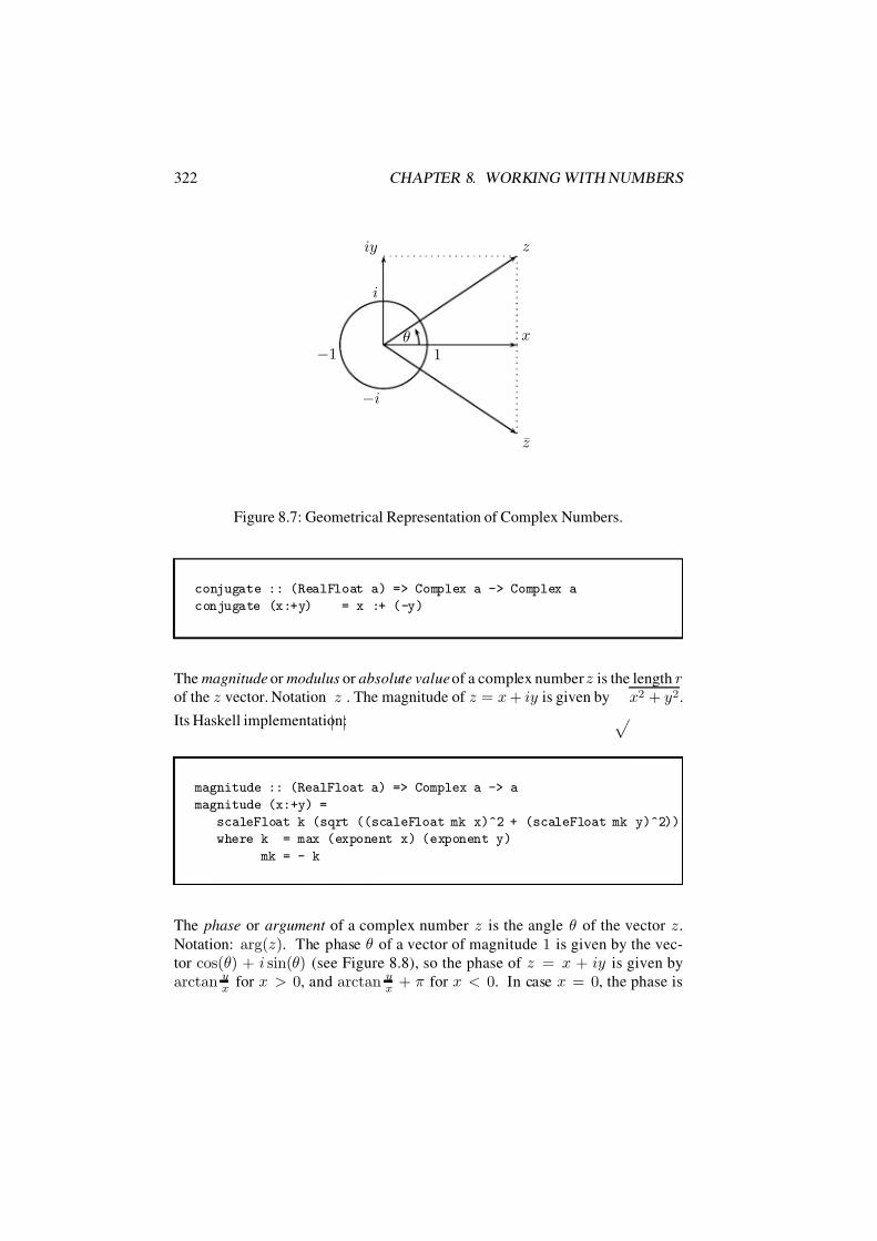
7/16/2019 The Haskell Road to Logic Maths and Programming
http://slidepdf.com/reader/full/the-haskell-road-to-logic-maths-and-programming-5634fa29ef7e9 333/448
322 CHAPTER 8. WORKING WITH NUMBERS
θ1−1
ziy
x
z
i
−i
Figure 8.7: Geometrical Representation of Complex Numbers.
conjugate :: (RealFloat a) => Complex a -> Complex a
conjugate (x:+y) = x :+ (-y)
The magnitude or modulus or absolute value of a complex number z is the length rof the z vector. Notation
|z
|. The magnitude of z = x + iy is given by x2 + y2.
Its Haskell implementation:
magnitude :: (RealFloat a) => Complex a -> a
magnitude (x:+y) =
scaleFloat k (sqrt ((scaleFloat mk x)^2 + (scaleFloat mk y)^2))
where k = max (exponent x) (exponent y)
mk = - k
The phase or argument of a complex number z is the angle θ of the vector z.
Notation: arg(z). The phase θ of a vector of magnitude 1 is given by the vec-
tor cos(θ) + i sin(θ) (see Figure 8.8), so the phase of z = x + iy is given by
arctan yx
for x > 0, and arctan yx
+ π for x < 0. In case x = 0, the phase is

7/16/2019 The Haskell Road to Logic Maths and Programming
http://slidepdf.com/reader/full/the-haskell-road-to-logic-maths-and-programming-5634fa29ef7e9 334/448
8.10. COMPLEX NUMBERS 323
θ
cos(θ)
i sin(θ)
ziy
x
Figure 8.8: ∠θ = cos(θ) + i sin(θ).

7/16/2019 The Haskell Road to Logic Maths and Programming
http://slidepdf.com/reader/full/the-haskell-road-to-logic-maths-and-programming-5634fa29ef7e9 335/448
324 CHAPTER 8. WORKING WITH NUMBERS
0. This computation is taken care of by the Haskell function atan2. Here is the
implementation:
phase :: (RealFloat a) => Complex a -> a
phase (0:+0) = 0
phase (x:+y) = atan2 y x
The polar representation of a complex number z = x + iy is r∠θ, where r = |z|and θ = arg(z). The advantage of polar representation is that complex multiplica-
tion looks much more natural: just multiply the magnitudes and add the phases.
(R∠ϕ)(r∠θ) = Rr∠(ϕ + θ).The polar representation of a complex number is given by:
polar :: (RealFloat a) => Complex a -> (a,a)
polar z = (magnitude z, phase z)
Note that polar representations are not unique, for we have:
. . . = r∠(θ − 2π) = r∠θ = r∠(θ + 2π) = r∠(θ + 4π) = . . .
To get from representation r∠θ to the representation as a vector sum of real andimaginary parts, use r∠θ = r(cos(θ) + i sin(θ)) (see again Figure 8.8). Imple-
mentation:
mkPolar :: (RealFloat a) => a -> a -> Complex a
mkPolar r theta = r * cos theta :+ r * sin theta
Converting a phase θ to a vector in the unit circle is done by:
cis :: (RealFloat a) => a -> Complex acis theta = cos theta :+ sin theta

7/16/2019 The Haskell Road to Logic Maths and Programming
http://slidepdf.com/reader/full/the-haskell-road-to-logic-maths-and-programming-5634fa29ef7e9 336/448
8.10. COMPLEX NUMBERS 325
The implementations of the arithmetical operations of addition, subtraction, mul-
tiplication, negation, absolute value and signum are given by:
instance (RealFloat a) => Num (Complex a) where
(x:+y) + (x’:+y’) = (x+x’) :+ (y+y’)
(x:+y) - (x’:+y’) = (x-x’) :+ (y-y’)
(x:+y) * (x’:+y’) = (x*x’-y*y’) :+ (x*y’+y*x’)
negate (x:+y) = negate x :+ negate y
abs z = magnitude z :+ 0
signum 0 = 0
signum z@(x:+y) = x/r :+ y/r where r = magnitude z
Note that the signum of a complex number z is in fact the vector representation
of arg(z). This suggests that arg(z) is a generalization of the + or − sign for
real numbers. That this is indeed the case can be seen when we perform complex
multiplication on real numbers: positive real numbers, represented in the complex
plane, have phase 0, or in general, phase 2kπ. Negative real number, represented
in the complex plane, have phase π, or in general, (2k + 1)π. Multiplying two
negative real numbers means multiplying their values and adding their phases, so
we get phase 2π, which is the same as phase 0, modulo 2kπ.
Complex division is the inverse of multiplication, so it boils down to performing
division on the magnitudes, and subtraction on the phases. The implementation in
terms of the vector representations looks slightly more involved than this, however:
instance (RealFloat a) => Fractional (Complex a) where
(x:+y) / (x’:+y’) = (x*x’’+y*y’’) / d :+ (y*x’’-x*y’’) / d
where x’’ = scaleFloat k x’
y’’ = scaleFloat k y’
k = - max (exponent x’) (exponent y’)
d = x’*x’’ + y’*y’’
For the definition of further numerical operations on complex numbers we refer to
the library file Complex.hs.
Complex numbers lose their mystery when one gets well acquainted with theirgeometrical representations. Here are some examples, for getting the feel of them.
The number 1 + i has magnitude√
2 and phase π4 : see Figure 8.9. Squaring

7/16/2019 The Haskell Road to Logic Maths and Programming
http://slidepdf.com/reader/full/the-haskell-road-to-logic-maths-and-programming-5634fa29ef7e9 337/448
326 CHAPTER 8. WORKING WITH NUMBERS
π4
1
i
√ 2
Figure 8.9: The number 1 + i.
π2
i
Figure 8.10: The number (1 + i)2.

7/16/2019 The Haskell Road to Logic Maths and Programming
http://slidepdf.com/reader/full/the-haskell-road-to-logic-maths-and-programming-5634fa29ef7e9 338/448
8.10. COMPLEX NUMBERS 327
3π4
2√ 2
Figure 8.11: The number (1 + i)3.

7/16/2019 The Haskell Road to Logic Maths and Programming
http://slidepdf.com/reader/full/the-haskell-road-to-logic-maths-and-programming-5634fa29ef7e9 339/448
328 CHAPTER 8. WORKING WITH NUMBERS
this number involves squaring the magnitude and doubling the phase, so (1 + i)2
has magnitude 2 and phase π2 : see Figure 8.10. Raising 1 + i to the third powerinvolves multiplying the magnitudes 2 and
√ 2 and adding the phases π
4 and π2 .
This gives magnitude 2√
2 and phase 3π4 . See Figure 8.11 for a picture of the
number (1+ i)3. Raising 1+ i to the fourth power involves squaring (1+ i)2, so themagnitude 2 is squared and the phase π
2 is doubled, which gives magnitude 4 and
phase π. Translating all of this back into vector sum notation, we get (1+i)2 = 2i,(1 + i)3 = −2 + 2i, and (1 + i)4 = −4. And sure enough, the Haskell libraryComplex.hs confirms these findings:
Complex> (1 :+ 1) 2
0.0 :+ 2.0
Complex> (1 :+ 1) 3
(-2.0) :+ 2.0
Complex> (1 :+ 1) 4(-4.0) :+ 0.0
Similarly, we see that multiplying i and −i involves multiplying the magnitudes1 and adding the phases π
2 and 3π2 , with result the number with magnitude 1 and
phase 2π = 0, i.e., the number 1. Here is the Haskell confirmation:
Complex> (0 :+ 1) * (0 :+ (-1))
1.0 :+ 0.0
Exercise 8.29 You are encouraged to familiarize yourself further with complex
numbers by checking the following by means of pictures:
1. Re(z) = 12 (z + z).
2. Im(z) = 12i (z − z).
3. tan(arg(z)) = Im(z)Re(z) .
4. R∠ϕr∠θ
= Rr∠(ϕ − θ).
5. arg(z1z2
) = arg(z1) − arg(z2).
6. arg( 1z ) = − arg(z).
Exercise 8.30 1. Use induction on n to prove De Moivre’s formula for n ∈ N:
(cos(ϕ) + i sin(ϕ))n = cos(nϕ) + i sin(nϕ).
Draw a picture to see what is happening!
7/16/2019 The Haskell Road to Logic Maths and Programming
http://slidepdf.com/reader/full/the-haskell-road-to-logic-maths-and-programming-5634fa29ef7e9 340/448
8.11. FURTHER READING 329
2. Prove De Moivre’s formula for exponents in Z by using the previous item,
plus:
(cos(ϕ) + i sin(ϕ))−m =1
(cos(ϕ) + i sin(ϕ))m.
8.11 Further Reading
A classic overview of the ideas and methods of mathematics, beautifully written,
and a book everyone with an interest in mathematics should possess and read is
Courant and Robbins [CR78, CrbIS96]. Here is praise for this book by Albert
Einstein:
A lucid representation of the fundamental concepts and methods of
the whole field of mathematics. It is an easily understandable intro-
duction for the layman and helps to give the mathematical student a
general view of the basic principles and methods.
Another beautiful book of numbers is [CG96]. For number theory and its history
see [Ore88].

7/16/2019 The Haskell Road to Logic Maths and Programming
http://slidepdf.com/reader/full/the-haskell-road-to-logic-maths-and-programming-5634fa29ef7e9 341/448
330 CHAPTER 8. WORKING WITH NUMBERS

7/16/2019 The Haskell Road to Logic Maths and Programming
http://slidepdf.com/reader/full/the-haskell-road-to-logic-maths-and-programming-5634fa29ef7e9 342/448
Chapter 9
Polynomials
Preview
Polynomials or integral rational functions are functions that can be represented by
a finite number of additions, subtractions, and multiplications with one indepen-
dent variable. The closed forms that we found and proved by induction for the
sums of evens, sums of odds, sums of squares, sums of cubes, and so on, in Chap-
ter 7, are all polynomial functions. In this chapter we will first study the process
of automating the search for polynomial functions that produce given sequences
of integers. Next, we establish the connection with the binomial theorem, we im-
plement a datatype for the polynomials themselves, and we use this datatype forthe study of combinatorial problems.
module POL
where
import Polynomials
331

7/16/2019 The Haskell Road to Logic Maths and Programming
http://slidepdf.com/reader/full/the-haskell-road-to-logic-maths-and-programming-5634fa29ef7e9 343/448
332 CHAPTER 9. POLYNOMIALS
9.1 Difference Analysis of Polynomial Sequences
Suppose an is a sequence of natural numbers, i.e., f = λn.an is a function in
N → N. The function f is a polynomial function of degree k if f can be presented
in the form
cknk + ck−1nk−1 + · · · + c1n + c0,
with ci ∈ Q and ck = 0.
Example 9.1 The sequence
[1, 4, 11, 22, 37, 56, 79, 106, 137, 172, 211, 254, 301, 352, . . .]
is given by the polynomial function f = λn.(2n2
+ n + 1). This is a function of the second degree.
Here is the Haskell check:
Prelude> take 15 (map (\ n -> 2*n^2 + n + 1) [0..])
[1,4,11,22,37,56,79,106,137,172,211,254,301,352,407]
Consider the difference sequence given by the function
d(f ) = λn.an+1
−an.
The Haskell implementation looks like this:
difs :: [Integer] -> [Integer]
difs [] = []
difs [n] = []
difs (n:m:ks) = m-n : difs (m:ks)
This gives:
POL> difs [1,4,11,22,37,56,79,106,137,172,211,254,301]
[3,7,11,15,19,23,27,31,35,39,43,47]

7/16/2019 The Haskell Road to Logic Maths and Programming
http://slidepdf.com/reader/full/the-haskell-road-to-logic-maths-and-programming-5634fa29ef7e9 344/448
9.1. DIFFERENCE ANALYSIS OF POLYNOMIAL SEQUENCES 333
The difference function d(f ) of a polynomial function f is itself a polynomial
function. E.g., if f = λn.(2n2 + n + 1), then:
d(f ) = λn.(2(n + 1)2 + (n + 1) + 1 − (2n2 + n + 1)
= λn.4n + 3.
The Haskell check:
POL> take 15 (map (\n -> 4*n + 3) [0..])
[3,7,11,15,19,23,27,31,35,39,43,47,51,55,59]
POL> take 15 (difs (map (\ n -> 2*n^2 + n + 1) [0..]))
[3,7,11,15,19,23,27,31,35,39,43,47,51,55,59]
Proposition 9.2 If f is a polynomial function of degree k then d(f ) is a polyno-
mial function of degree k − 1.
Proof. Suppose f (n) is given by
cknk + ck−1nk−1 + · · · + c1n + c0.
Then d(f )(n) is given by
ck(n + 1)k+ck−1(n + 1)k−1 + · · · + c1(n + 1) + c0
− (cknk + ck−1nk−1 + · · · + c1n + c0).
It is not hard to see that f (n + 1) has the form cknk + g(n), with g a polynomial
of degree k − 1. Since f (n) also is of the form cknk + h(n), with h a polynomial
of degree k − 1, d(f )(n) has the form g(n) − h(n), so d(f ) is itself a polynomialof degree k − 1.
It follows from Proposition 9.2 that if f is a polynomial function of degree k, then
dk(f ) will be a constant function (a polynomial function of degree 0).
Here is a concrete example of computing difference sequences until we hit at a
constant sequence:
-12 -11 6 45 112 213 354 541
1 17 39 67 101 141 187
16 22 28 34 40 46
6 6 6 6 6
We find that the sequence of third differences is constant, which means that the
form of the original sequence is a polynomial of degree 3. To find the next number

7/16/2019 The Haskell Road to Logic Maths and Programming
http://slidepdf.com/reader/full/the-haskell-road-to-logic-maths-and-programming-5634fa29ef7e9 345/448
334 CHAPTER 9. POLYNOMIALS
in the sequence, just take the sum of the last elements of the rows. This gives
6 + 46 + 187 + 541 = 780.
Charles Babbage (1791–1871), one of the founding fathers of computer science,
used these observations in the design of his difference engine. We will give a
Haskell version of the machine.
According to Proposition 9.2, if a given input list has a polynomial form of degreek, then after k steps of taking differences the list is reduced to a constant list:
POL> difs [-12,-11,6,45,112,213,354,541,780,1077]
[1,17,39,67,101,141,187,239,297]
POL> difs [1,17,39,67,101,141,187,239,297]
[16,22,28,34,40,46,52,58]
POL> difs [16,22,28,34,40,46,52,58]
[6,6,6,6,6,6,6]
The following function keeps generating difference lists until the differences get
constant:
difLists :: [[Integer]]->[[Integer]]
difLists [] = []
difLists lists@(xs:xss) =
if constant xs then lists else difLists ((difs xs):lists)
where
constant (n:m:ms) = all (==n) (m:ms)
constant _ = error "lack of data or not a polynomial fct"
This gives the lists of all the difference lists that were generated from the initialsequence, with the constant list upfront.
POL> difLists [[-12,-11,6,45,112,213,354,541,780,1077]]
[[6,6,6,6,6,6,6],
[16,22,28,34,40,46,52,58],
[1,17,39,67,101,141,187,239,297],
[-12,-11,6,45,112,213,354,541,780,1077]]
The list of differences can be used to generate the next element of the original
sequence: just add the last elements of all the difference lists to the last element of
the original sequence. In our example case, to get the next element of the list
[−12, −11, 6, 45, 112, 213, 354, 541, 780, 1077]
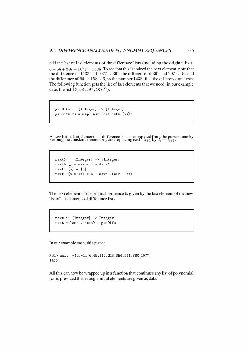
7/16/2019 The Haskell Road to Logic Maths and Programming
http://slidepdf.com/reader/full/the-haskell-road-to-logic-maths-and-programming-5634fa29ef7e9 346/448
9.1. DIFFERENCE ANALYSIS OF POLYNOMIAL SEQUENCES 335
add the list of last elements of the difference lists (including the original list):
6 + 58+ 297 + 1077 = 1438. To see that this is indeed the next element, note thatthe difference of 1438 and 1077 is 361, the difference of 361 and 297 is 64, and
the difference of 64 and 58 is 6, so the number 1438 ‘fits’ the difference analysis.
The following function gets the list of last elements that we need (in our example
case, the list [6,58,297,1077]):
genDifs :: [Integer] -> [Integer]
genDifs xs = map last (difLists [xs])
A new list of last elements of difference lists is computed from the current one bykeeping the constant element d1, and replacing each di+1 by di + di+1.
nextD :: [Integer] -> [Integer]
nextD [] = error "no data"
nextD [n] = [n]
nextD (n:m:ks) = n : nextD (n+m : ks)
The next element of the original sequence is given by the last element of the new
list of last elements of difference lists:
next :: [Integer] -> Integer
next = last . nextD . genDifs
In our example case, this gives:
POL> next [-12,-11,6,45,112,213,354,541,780,1077]
1438
All this can now be wrapped up in a function that continues any list of polynomial
form, provided that enough initial elements are given as data:

7/16/2019 The Haskell Road to Logic Maths and Programming
http://slidepdf.com/reader/full/the-haskell-road-to-logic-maths-and-programming-5634fa29ef7e9 347/448
336 CHAPTER 9. POLYNOMIALS
continue :: [Integer] -> [Integer]continue xs = map last (iterate nextD differences)
where
differences = nextD (genDifs xs)
This uses the predefined Haskell function iterate, that is given by:
iterate :: (a -> a) -> a -> [a]
iterate f x = x : iterate f (f x)
This is what we get:
POL> take 20 (continue [-12,-11,6,45,112,213,354,541,780,1077])
[1438,1869,2376,2965,3642,4413,5284,6261,7350,8557,9888,11349,
12946,14685,16572,18613,20814,23181,25720,28437]
If a given list is generated by a polynomial, then the degree of the polynomial can
be computed by difference analysis, as follows:
degree :: [Integer] -> Int
degree xs = length (difLists [xs]) - 1
The difference engine is smart enough to be able to continue a list of sums of
squares, or a list of sums of cubes:
POL> take 10 (continue [1,5,14,30,55])
[91,140,204,285,385,506,650,819,1015,1240]
POL> take 10 (continue [1,9,36,100,225,441])
[784,1296,2025,3025,4356,6084,8281,11025,14400,18496]
Exercise 9.3 What continuation do you get for [3,7,17,39,79,143]? Can you
reconstruct the polynomial function that was used to generate the sequence?

7/16/2019 The Haskell Road to Logic Maths and Programming
http://slidepdf.com/reader/full/the-haskell-road-to-logic-maths-and-programming-5634fa29ef7e9 348/448
9.2. GAUSSIAN ELIMINATION 337
Difference analysis yields an algorithm for continuing any finite sequence with a
polynomial form. Is it also possible to give an algorithm for finding the form? Thiswould solve the problem of how to guess the closed forms for the functions that
calculate sums of squares, sums of cubes, and so on. The answer is ‘yes’, and the
method is Gaussian elimination.
9.2 Gaussian Elimination
If we know that a sequence a0, a1, a2, a3, . . . has a polynomial form of degree
3, then we know that the form is a + bx + cx2 + dx3 (listing the coefficients
in increasing order). This means that we can find the form of the polynomial by
solving the following quadruple of linear equations in a,b,c,d:
a = a0
a + b + c + d = a1
a + 2b + 4c + 8d = a2
a + 3b + 9c + 27d = a3
Since this is a set of four linear equations in four unknowns, where the equations
are linearly independent (none of them can be written as a multiple of any of the
others), this can be solved by eliminating the unknowns one by one.
Example 9.4 Find the appropriate set of equations for the sequence
[−7, −2, 15, 50, 109, 198, 323]
and solve it.
Difference analysis yields that the sequence is generated by a polynomial of the
third degree, so the sequence leads to the following set of equations:
a = −7
a + b + c + d = −2
a + 2b + 4c + 8d = 15
a + 3b + 9c + 27d = 50
Eliminating a and rewriting gives:
b + c + d = 5
2b + 4c + 8d = 22
3b + 9c + 27d = 57

7/16/2019 The Haskell Road to Logic Maths and Programming
http://slidepdf.com/reader/full/the-haskell-road-to-logic-maths-and-programming-5634fa29ef7e9 349/448
338 CHAPTER 9. POLYNOMIALS
Next, eliminate the summand with factor d from the second and third equation.
Elimination from the second equation is done by subtracting the second equationfrom the 8-fold product of the first equation. This gives 6b + 4c = 18, which
can be simplified to 3b + 2c = 9. Elimination from the third equation is done
by subtracting the third equation from the 27-fold product of the first, with result
24b + 18c = 78. We get the following pair of equations:
3b + 2c = 9
24b + 18c = 78
Elimination of c from this pair is done by subtracting the second equation from
the 9-fold product of the first. This gives 3b = 3, whence b = 1. Together with
3b + 2c = 9 we get c = 3. Together with b + c + d = 5 we get d = 1. Thus, the
polynomial we are looking for has the form λn.(n3 + 3n2 + n
−7).
Exercise 9.5 Find the appropriate set of equations for the sequence
[13, 21, 35, 55, 81, 113, 151]
and solve it.
Solving sets of linear equations can be viewed as manipulation of matrices of
coefficients. E.g., the quadruple of linear equations in a,b,c,d for a polynomial of
the third degree gives the following matrix:
1 0 0 0 a0
1 1 1 1 a1
1 2 4 8 a2
1 3 9 27 a3
To solve this, we transform it to an equivalent matrix in so-called echelon form or
left triangular form, i.e., a matrix of the form:
a00 a01 a02 a03 b0
0 a11 a12 a13 b1
0 0 a22 a23 b2
0 0 0 a33 b3
From this form, compute the value of variable d from the last row, next eliminate
this variable from the third row, and find the value of c. Then use the values of
d and c to find the value of b from the second row, and finally, use the values of
b,c,d to find the value of a from the first row.
To handle matrices, the following type declarations are convenient.

7/16/2019 The Haskell Road to Logic Maths and Programming
http://slidepdf.com/reader/full/the-haskell-road-to-logic-maths-and-programming-5634fa29ef7e9 350/448
9.2. GAUSSIAN ELIMINATION 339
type Matrix = [Row]type Row = [Integer]
It is also convenient to be able to have functions for the numbers of rows and
columns of a matrix.
rows, cols :: Matrix -> Int
rows m = length m
cols m | m == [] = 0
| otherwise = length (head m)
The function genMatrix produces the appropriate matrix for a list generated by a
polynomial:
genMatrix :: [Integer] -> Matrix
genMatrix xs = zipWith (++) (genM d) [ [x] | x <- xs ]
where
d = degree xs
genM n = [ [ (toInteger x^m) | m <- [0..n] ] | x <- [0..n] ]
zipWith is predefined in the Haskell prelude as follows:
zipWith :: (a->b->c) -> [a]->[b]->[c]
zipWith z (a:as) (b:bs) = z a b : zipWith z as bs
zipWith _ _ _ = []
In a picture:
[(z x0 y0), (z x1 y1), . . . , (z xn yn), [xn+1, xn+2, . . .
[yn+1, yn+2, . . .

7/16/2019 The Haskell Road to Logic Maths and Programming
http://slidepdf.com/reader/full/the-haskell-road-to-logic-maths-and-programming-5634fa29ef7e9 351/448
340 CHAPTER 9. POLYNOMIALS
genMatrix gives, e.g.:
POL> genMatrix [-7,-2,15,50,109,198,323]
[[1,0,0,0,-7],[1,1,1,1,-2],[1,2,4,8,15],[1,3,9,27,50]]
The process of transforming the matrix to echelon form is done by so-called for-
ward elimination: use one row to eliminate the first coefficient from the other rows
by means of the following process of adjustment (the first row is used to adjust the
second one):
adjustWith :: Row -> Row -> Row
adjustWith (m:ms) (n:ns) = zipWith (-) (map (n*) ms) (map (m*) ns)
To transform a matrix into echelon form, proceed as follows:
1. If the number of rows or the number of columns of the matrix is 0, then the
matrix is already in echelon form.
2. If every row of rs begins with a 0 then the echelon form of rs can be found
by putting 0’s in front of the echelon form of map tail rs.
3. If rs has rows that do not start with a 0, then take the first one of these, piv,
and use it to eliminate the leading coefficients from the other rows. This
gives a matrix of the form
a00 a01 a02 a03 · · · b00 a11 a12 a13 · · · b1
0 a21 a22 a23 · · · b2
0 a31 a32 a33 · · · b3
......
......
......
0 an1 an2 an3 · · · bn
where the first row is the pivot row. All that remains to be done in this case
is to put the following sub matrix in echelon form:
a11 a12 a13 · · · b1
a21 a22 a23 · · · b2
a31 a32 a33 · · · b3
.
.....
.
.....
.
..an1 an2 an3 · · · bn

7/16/2019 The Haskell Road to Logic Maths and Programming
http://slidepdf.com/reader/full/the-haskell-road-to-logic-maths-and-programming-5634fa29ef7e9 352/448
9.2. GAUSSIAN ELIMINATION 341
The code for this can be found in the Haskell demo file Matrix.hs (part of the Hugs
system):
echelon :: Matrix -> Matrix
echelon rs
| null rs || null (head rs) = rs
| null rs2 = map (0:) (echelon (map tail rs))
| otherwise = piv : map (0:) (echelon rs’)
where rs’ = map (adjustWith piv) (rs1++rs3)
(rs1,rs2) = span leadZero rs
leadZero (n:_) = n==0
(piv:rs3) = rs2
Here is an example:
POL> echelon [[1,0,0,0,-7],[1,1,1,1,-2],[1,2,4,8,15],[1,3,9,27,50]]
[[1,0,0,0,-7],[0,-1,-1,-1,-5],[0,0,-2,-6,-12],[0,0,0,-12,-12]]
Backward Gaussian elimination, or computing the values of the variables from a
matrix in echelon form, is done by computing the value of the variable in the lastrow, eliminate that variable from the other rows to get a smaller matrix in echelon
form, and repeating that process until the values of all variables are found. If
we know that ax = c (we may assume a = 0), and the coordinate of x is the
coordinate ain = b of ai1 | · · · | ain−1 | ain | d, then we can eliminate this
coordinate by replacing ai1 | · · · | ain−1 | ain | d with the following:
a · ai1 | · · · | a · ain−1 | ad − bc.
It does make sense to first reduce x = c/a to its simplest form by dividing out
common factors of c and a. The implementation of rational numbers does this
for us if we express x as a number of type Rational (see Section 8.6 for further
details). Note that an elimination step transforms a matrix in echelon form, minus
its last row, into a smaller matrix in echelon form. Here is the implementation:
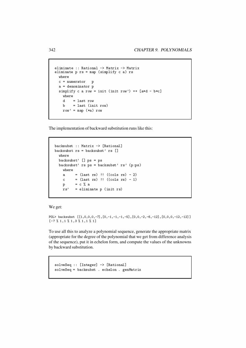
7/16/2019 The Haskell Road to Logic Maths and Programming
http://slidepdf.com/reader/full/the-haskell-road-to-logic-maths-and-programming-5634fa29ef7e9 353/448
342 CHAPTER 9. POLYNOMIALS
eliminate :: Rational -> Matrix -> Matrixeliminate p rs = map (simplify c a) rs
where
c = numerator p
a = denominator p
simplify c a row = init (init row’) ++ [a*d - b*c]
where
d = last row
b = last (init row)
row’ = map (*a) row
The implementation of backward substitution runs like this:
backsubst :: Matrix -> [Rational]
backsubst rs = backsubst’ rs []
where
backsubst’ [] ps = ps
backsubst’ rs ps = backsubst’ rs’ (p:ps)
where
a = (last rs) !! ((cols rs) - 2)
c = (last rs) !! ((cols rs) - 1)
p = c % a
rs’ = eliminate p (init rs)
We get:
POL> backsubst [[1,0,0,0,-7],[0,-1,-1,-1,-5],[0,0,-2,-6,-12],[0,0,0,-12,-12] ]
[-7 % 1,1 % 1,3 % 1,1 % 1]
To use all this to analyze a polynomial sequence, generate the appropriate matrix
(appropriate for the degree of the polynomial that we get from difference analysis
of the sequence), put it in echelon form, and compute the values of the unknowns
by backward substitution.
solveSeq :: [Integer] -> [Rational]
solveSeq = backsubst . echelon . genMatrix

7/16/2019 The Haskell Road to Logic Maths and Programming
http://slidepdf.com/reader/full/the-haskell-road-to-logic-maths-and-programming-5634fa29ef7e9 354/448
9.2. GAUSSIAN ELIMINATION 343
Recall that the sequence of sums of squares starts as follows: 0, 1, 5, 14, 30, . . ..
Solving this sequence with solveSeq gives:
POL> solveSeq [0,1,5,14,30]
[0 % 1,1 % 6,1 % 2,1 % 3]
This gives the form
1
3n3 +
1
2n2 +
1
6n =
2n3 + 3n2 + n
6=
n(n + 1)(2n + 1)
6.
Here is a Haskell check (the use of the / operator creates a list of Fractionals):
POL> map (\ n -> (1/3)*n^3 + (1/2)*n^2 + (1/6)*n) [0..4]
[0.0,1.0,5.0,14.0,30.0]
Similarly, 0, 1, 9, 36, 100, 225 is the start of the sequence of sums of cubes. Solvingthis with solveSeq gives:
POL> solveSeq [0, 1, 9, 36, 100, 225]
[0 % 1,0 % 1,1 % 4,1 % 2,1 % 4]
This gives the form
1
4n4 +
1
2n3 +
1
4n2 =
n4 + 2n3 + n2
4=
n2(n + 1)2
4=
n(n + 1)
2
2
.
The running example from the previous section is solved as follows:
POL> solveSeq [-12,-11,6,45,112,213,354,541,780,1077]
[-12 % 1,-5 % 1,5 % 1,1 % 1]
Thus, the sequence has the form n3 + 5n2 − 5n − 12.
Before we look at the confirmation, let us note that we are now in fact using rep-
resentations of polynomial functions as lists of their coefficients, starting from the
constant coefficient. It is easy to implement a conversion from these representa-
tions to the polynomial functions that they represent:
p2fct :: Num a => [a] -> a -> a
p2fct [] x = 0
p2fct (a:as) x = a + (x * p2fct as x)
We can use this in the confirmations, as follows:
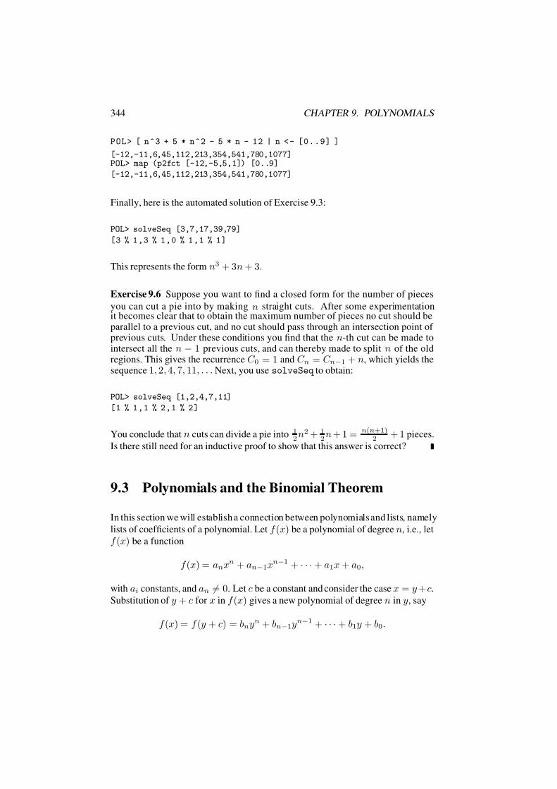
7/16/2019 The Haskell Road to Logic Maths and Programming
http://slidepdf.com/reader/full/the-haskell-road-to-logic-maths-and-programming-5634fa29ef7e9 355/448
344 CHAPTER 9. POLYNOMIALS
POL> [ n^3 + 5 * n^2 - 5 * n - 12 | n <- [0..9] ]
[-12,-11,6,45,112,213,354,541,780,1077]POL> map (p2fct [-12,-5,5,1]) [0..9]
[-12,-11,6,45,112,213,354,541,780,1077]
Finally, here is the automated solution of Exercise 9.3:
POL> solveSeq [3,7,17,39,79]
[3 % 1,3 % 1,0 % 1,1 % 1]
This represents the form n3 + 3n + 3.
Exercise 9.6 Suppose you want to find a closed form for the number of pieces
you can cut a pie into by making n straight cuts. After some experimentationit becomes clear that to obtain the maximum number of pieces no cut should beparallel to a previous cut, and no cut should pass through an intersection point of previous cuts. Under these conditions you find that the n-th cut can be made tointersect all the n − 1 previous cuts, and can thereby made to split n of the oldregions. This gives the recurrence C 0 = 1 and C n = C n−1 + n, which yields thesequence 1, 2, 4, 7, 11, . . . Next, you use solveSeq to obtain:
POL> solveSeq [1,2,4,7,11]
[1 % 1,1 % 2,1 % 2]
You conclude that n cuts can divide a pie into 12
n2 + 12
n + 1 = n(n+1)2 + 1 pieces.
Is there still need for an inductive proof to show that this answer is correct?
9.3 Polynomials and the Binomial Theorem
In this section we will establish a connection between polynomials and lists, namely
lists of coefficients of a polynomial. Let f (x) be a polynomial of degree n, i.e., let
f (x) be a function
f (x) = anxn + an−1xn−1 + · · · + a1x + a0,
with ai constants, and an = 0. Let c be a constant and consider the case x = y + c.
Substitution of y + c for x in f (x) gives a new polynomial of degree n in y, say
f (x) = f (y + c) = bnyn + bn−1yn−1 + · · · + b1y + b0.

7/16/2019 The Haskell Road to Logic Maths and Programming
http://slidepdf.com/reader/full/the-haskell-road-to-logic-maths-and-programming-5634fa29ef7e9 356/448
9.3. POLYNOMIALS AND THE BINOMIAL THEOREM 345
a = 0,
(a · f (x)) = a · f (x),
(xn) = nxn−1
,
(f (x) ± g(x)) = f (x) ± g(x),
(f (x) · g(x)) = f (x)g(x) + f (x)g
(x)b,
(f (g(x))) = g(x) · f (g(x)).
Figure 9.1: Differentiation Rules.
To consider an example, take f (x) = 3x4 − x + 2, and let c = −1. Substituting
y + c for x we get:
f (x) = f (y + c) = f (y − 1)
= 3(y − 1)4 − (y − 1) + 2
= (3y4 − 12y3 + 18y2 − 12y + 3) − (y − 1) + 2
= 3y4 − 12y3 + 18y2 − 13y + 6.
We will see shortly that the coefficients bi can be computed in a very simple way.
Substitution of x−
c for y in in f (y + c) gives
f (x) = bn(x − c)n + bn−1(x − c)n−1 + · · · + b1(x − c) + b0.
Calculation of f (x), f (x), . . . , f (n)(x) (the first, second, .. . , n-th derivative of
f ), is done with the familiar rules of Figure 9.1.1 In particular, this gives (b(x −c)k) = kb(x − c)k−1, and we get:
f (x) = b1 + 2b2(x − c) + · · · + nbn(x − c)n−1
f (x) = 2b2 + 3 · 2b3(x − c) + · · · + n(n − 1)bn(x − c)n−2
...
f (n)(x) = n(n
−1)(n
−2)
· · ·3
·2bn.
1If these rules are unfamiliar to you, or if you need to brush up your knowledge of analysis, you
should consult a book like [Bry93].

7/16/2019 The Haskell Road to Logic Maths and Programming
http://slidepdf.com/reader/full/the-haskell-road-to-logic-maths-and-programming-5634fa29ef7e9 357/448
346 CHAPTER 9. POLYNOMIALS
Substitution of x = c gives:
f (c) = b0, f (c) = b1, f (c) = 2b2, . . . , f (n)(c) = n!bn.
This yields the following instruction for calculating the bk:
b0 = f (c), b1 = f (c), b2 =f (c)
2, . . . , bn =
f (n)(c)
n!.
In general:
bk =f (k)(c)
k!.
Applying this to the example f (x) = 3x4 − x + 2, with c = −1, we see that
b0 = f (−1) = 3(−1)4 + 1 + 2 = 6, b1 = f (−1) = 12(−1)3 − 1 = −13,
b2 =f (−1)
2=
36(−1)2
2= 18, b3 =
f (3)(−1)
6= −72
6=
−12, b4 =
f (4)(−1)
24= 3.
Another example is the expansion of (z + 1)n. Using the calculation method with
derivatives, we get, for c = 0:
f (z) = (z + 1)n = bnzn + bn−1zn−1 + · · · + b1z + b0,
with the following derivatives:
f (z) = n(z + 1)n−1, f (z) = n(n − 1)(z + 1)n−2, . . . , f (n)(z) = n!.
Substituting z = 0 this gives:
b0 = 1, b1 = n, b2 = n(n−1)2 , · · · , bk = n(n−1)···(n−k+1)
k! , · · · , bn = n!n! = 1.
The general coefficient bk has the form
bk =n(n − 1) · · · (n − k + 1)
k!=
n(n − 1) · · · (n − k + 1)
k!· (n − k)!
(n − k)!
=n!
k! (n − k)!.
Define: n
k
:=
n!
k! (n − k)!.
Pronouncenk
as ‘n choose k’ or ‘n over k’. We have derived:
Theorem 9.7 (Newton’s binomial theorem)
(z + 1)n =nk=0
nkzk.
7/16/2019 The Haskell Road to Logic Maths and Programming
http://slidepdf.com/reader/full/the-haskell-road-to-logic-maths-and-programming-5634fa29ef7e9 358/448
9.3. POLYNOMIALS AND THE BINOMIAL THEOREM 347
If A is a set of n objects, then there are nk ways to pick a subset B from A with
|B| = k. Thus, nk is also the number of k-sized subsets of an n-sized set. To
see why this is so, note that the number of k-sequences picked from A, without
repetitions, equals
n · (n − 1) · · · · · (n − k + 1),
for there are n ways to pick the first element in the sequence, n − 1 ways to pick
the second element in the sequence, . . . , and n − (k − 1) ways to pick the k-th
element in the sequence. The number n · (n − 1) · · · · · (n − k + 1) is equal ton!
(n−k)! .
For picking k-sized subsets from A, order does not matter. There are k! ways
of arranging sequences of size k without repetition. These are all equivalent. This
gives n!k! (n−k)! for the number of k-sized subsets of a set of size n. This connection
explains the phrasing ‘n choose k’.
Note the following:n
0
= 1,
n
1
= n,
n
2
=
n(n − 1)
2,
n
3
=
n(n − 1)(n − 2)
6.
Here is a straightforward implementation of nk
.
choose n k = (product [(n-k+1)..n]) ‘div‘ (product [1..k])
The more general version of Newton’s binomial theorem runs:
Theorem 9.8 (Newton’s binomial theorem, general version)
(x + y)n =nk=0
n
k
xkyn−k.
Note: a binomial is the sum of two terms, so (x + y) is a binomial.
Proof: To get this from the special case (z + 1)n =n
k=0
nk
zk derived above,
set z = xy
to get (xy + 1)n =n
k=0
nk
xk
yk, and multiply by yn:
(x + y)n =
x
y+ 1
n· yn
= nk=0
nk
xk
yk
· yn =
nk=0
nk
xk · yn
yk=
nk=0
nk
xkyn−k.

7/16/2019 The Haskell Road to Logic Maths and Programming
http://slidepdf.com/reader/full/the-haskell-road-to-logic-maths-and-programming-5634fa29ef7e9 359/448
348 CHAPTER 9. POLYNOMIALS
Because of their use in the binomial theorem, the numbers nk are called binomial
coefficients. What the binomial theorem gives us is:
(x + y)0 = 1x0y0
(x + y)1 = 1x1y0 + 1x0y1
(x + y)2 = 1x2y0 + 2x1y1 + 1x0y2
(x + y)3 = 1x3y0 + 3x2y1 + 3x1y2 + 1x0y3
(x + y)4 = 1x4y0 + 4x3y1 + 6x2y2 + 4x1y3 + 1x0y4
(x + y)5 = 1x5y0 + 5x4y1 + 10x3y2 + 10x2y3 + 5x1y4 + 1x0y5
...
To see how this pattern arises, look at what happens when we raise x + y to the
n-th power by performing the n multiplication steps to work out the product of
(x + y)(x + y) · · · (x + y) n factors
:
x + yx + y ×
x2 + xy + xy + y2
x + y ×x3 + x2y + x2y + x2y + xy2 + xy2 + xy2 + y3
x + y ×...
Every term in this expansion is itself the product of x-factors and y-factors, with
a total number of factors always n, so that each term has the form xkyn−k. Every
binomial (x+y) in (x+n)n either contributes an x-factor or a y-factor to xkyn−k.
The number of ways to get at the term xkyn−k equals the number of k-sized sub-
sets from a set of size n (pick any subset of k binomials from the set of n binomial
factors). Thus, this term occurs exactlynk
times.
We can arrange the binomial coefficients in the well-known triangle of Pascal.00
10
11
20
21
22
30 3
1 32 3
340 41
42 43
44
...

7/16/2019 The Haskell Road to Logic Maths and Programming
http://slidepdf.com/reader/full/the-haskell-road-to-logic-maths-and-programming-5634fa29ef7e9 360/448
9.3. POLYNOMIALS AND THE BINOMIAL THEOREM 349
Working this out, we get:
11 1
1 2 11 3 3 1
1 4 6 4 1...
Studying the pattern of Pascal’s triangle, we see that that it is built according to the
following law: n
k
=
n − 1
k − 1
+
n − 1
k
.
This is called the addition law for binomial coefficients. To see that this law iscorrect, consider a set A of size n, and single out one of its objects, a. To count
the number of ways of picking a k-sized subset B from A, consider the two cases
(i) a ∈ B and (ii) a /∈ B. The number of ways of picking a k-sized subset B from
A with a ∈ B is equal to the number of ways of picking a k − 1-sized subset from
A − a, i.e.,n−1k−1
. The number of ways of picking a k-sized subset B from
A with a /∈ B is equal to the number of ways of picking a k-sized subset from
A − a, i.e.,n−1k
. Thus, there are
n−1k−1
+n−1k
ways of picking a k-sized
subset from an n-sized set.
It is of course also possible to prove the addition law directly from the definition
of nk
. Assume k > 0. Then:
n
−1
k − 1 +n
−1
k =
(n
−1)!
(k − 1)! (n − k)! +
(n
−1)!
k! (n − 1 − k)!
=(n − 1)! k
k! (n − k)!+
(n − 1)! (n − k)
k! (n − k)!
=(n − 1)! n
k! (n − k)!=
n!
k! (n − k)!=
n
k
.
We can use the addition law for an implementation of nk
. In accordance with
the interpretation of nk
as the number of k-sized subset of an n-sized set, we
will putn0
= 1 (there is just one way to pick a 0-sized subset from any set) and
nk
= 0 for n < k (no ways to pick a k-sized subset from a set that has less
than k elements). A further look at Pascal’s triangle reveals the following law of
symmetry: n
k
=
n
n − k
.

7/16/2019 The Haskell Road to Logic Maths and Programming
http://slidepdf.com/reader/full/the-haskell-road-to-logic-maths-and-programming-5634fa29ef7e9 361/448
350 CHAPTER 9. POLYNOMIALS
This makes sense under the interpretation of nk as the number of k-sized subsets
of a set of size n, for the number of k-sized subsets equals the number of theircomplements. There is just one way to pick an n-sized subset from an n-sized set
(pick the whole set), sonn
= 1. This leads to the following implementation:
choose’ n 0 = 1
choose’ n k | n < k = 0
| n == k = 1
| otherwise =
choose’ (n-1) (k-1) + (choose’ (n-1) (k))
Exercise 9.9 Which implementationis more efficient, choose or choose’? Why?
Exercise 9.10 Derive the symmetry law for binomial coefficients directly from
the definition.
We will now give an inductive proof of Newton’s binomial theorem. The proof
uses the addition law for binomials, in the formnk−1
+nk
=n+1k
.
Theorem 9.11 (Newton’s binomial theorem again)
(x + y)n =
nk=0
n
k
xkyn−k.
Proof. Induction on n.
Basis:
(x + y)0 = 1 =
0
0
x0y0 =
0k=0
0
k
xky0−k.
Induction step: Assume
(x + y)n =nk=0
nk
xkyn−k.

7/16/2019 The Haskell Road to Logic Maths and Programming
http://slidepdf.com/reader/full/the-haskell-road-to-logic-maths-and-programming-5634fa29ef7e9 362/448
9.3. POLYNOMIALS AND THE BINOMIAL THEOREM 351
Then:
(x + y)n+1 = (x + y)(x + y)n
ih= (x + y)
nk=0
n
k
xkyn−k
= xnk=0
n
k
xkyn−k + y
nk=0
n
k
xkyn−k
=
nk=0
n
k
xk+1yn−k +
nk=0
n
k
xky(n+1)−k
= xn+1 +n−1
k=0n
kxk+1yn−k +
n
k=1n
kxky(n+1)−k + yn+1
= xn+1 +
nk=1
n
k − 1
xky(n+1)−k +
nk=1
n
k
xky(n+1)−k + yn+1
= xn+1 +nk=1
n
k − 1
xky(n+1)−k +
n
k
xky(n+1)−k
+ yn+1
add= xn+1 +
nk=1
n + 1
k
xky(n+1)−k + yn+1
=
n+1k=1
n + 1
k
xky(n+1)−k + yn+1 =
n+1k=0
n + 1
k
xky(n+1)−k.
Exercise 9.12 Show from the definition that if 0 < k n then:n
k
=
n
k·
n − 1
k − 1
.
The law from exercise 9.12 is the so-called absorption law for binomial coeffi-
cients. It allows for an alternative implementation of a function for binomial coef-
ficients, for we have the following recursion:
n
0 = 1, n
k = 0 for n < k, n
k =n
k ·n − 1
k − 1 for 0 < k n.
Thus we get a more efficient function fornk
:

7/16/2019 The Haskell Road to Logic Maths and Programming
http://slidepdf.com/reader/full/the-haskell-road-to-logic-maths-and-programming-5634fa29ef7e9 363/448
352 CHAPTER 9. POLYNOMIALS
binom n 0 = 1binom n k | n < k = 0
| otherwise = (n * binom (n-1) (k-1)) ‘div‘ k
Exercise 9.13 Use a combinatorial argument (an argument in terms of sizes the
subsets of a set) to prove Newton’s law:n
m
·
m
k
=
n
k
·
n − k
m − k
.
Exercise 9.14 Prove:n
n
+
n + 1
n
+
n + 2
n
+ · · · +
n + k
n
=
n + k + 1
n + 1
.
9.4 Polynomials for Combinatorial Reasoning
To implement the polynomial functions in a variable z, we will represent a poly-
nomial
f (z) = f 0 + f 1z + f 2z2 +· · ·
+ f n−
1zn−1 + f nzn
as a list of its coefficients:
[f 0, f 1, . . . , f n].
As we have seen, the function p2fct maps such lists to the corresponding func-
tions.
The constant zero polynomial has the form f (z) = 0. In general we will avoid
trailing zeros in the coefficient list, i.e., we will assume that if n > 0 then f n = 0.
The constant function λz.c will get represented as [c], so there is a map from in-
tegers to polynomial representations, given by λc.[c]. We will also allow rationals
as coefficients, to there is also a map from rationals to polynomial representations,
given by λr.[r].
We need some conventions for switching back and forth between a polynomial and
its list of coefficients. If f (z) is a polynomial, then we use f for its coefficient list.
If this list of coefficients is non-empty then, as before, we will indicate the tail of f
7/16/2019 The Haskell Road to Logic Maths and Programming
http://slidepdf.com/reader/full/the-haskell-road-to-logic-maths-and-programming-5634fa29ef7e9 364/448
9.4. POLYNOMIALS FOR COMBINATORIAL REASONING 353
as f . Thus, if f = [f 0, f 1, . . . , f n], then f = [f 1, . . . , f n], and we have the identity
f = f 0 : f . Moreover, if f (z) = f 0 + f 1z + f 2z2 + · · · + f n−1zn−1 + f nzn, thenwe use f (z) for f 1 + f 2z + · · · + f n−1zn−2 + f nzn−1. This convention yields the
following important equality:
f (z) = f 0 + zf (z).
The identity function λz.z will get represented as [0, 1], for this function is of the
form λz.f 0 + f 1z, with f 0 = 0 and f 1 = 1. This gives:
z :: Num a => [a]
z = [0,1]
To negate a polynomial, simply negate each term in its term expansion. For if
f (z) = f 0 + f 1z + f 2z2 + · · · , then −f (z) = −f 0 −f 1z −f 2z2 − · · · . This gives:
negate [] = []
negate (f:fs) = (negate f) : (negate fs)
To add two polynomials f (z) and g(z), just add their coefficients, for clearly, if
f (z) = f 0 + f 1z + f 2z2 + · · ·+ f kzk and g(z) = b0 + b1z + g2z2 + · · · = gmzm,
then
f (z) + g(z) = (f 0 + g0) + (f 1 + g1)z + (f 2 + g2)z2 + · · ·This translates into Haskell as follows:
fs + [] = fs
[] + gs = gs
(f:fs) + (g:gs) = f+g : fs+gs
Note that this uses overloading of the + sign: in f+g we have addition of numbers,
in fs+gs addition of polynomial coefficient sequences.

7/16/2019 The Haskell Road to Logic Maths and Programming
http://slidepdf.com/reader/full/the-haskell-road-to-logic-maths-and-programming-5634fa29ef7e9 365/448
354 CHAPTER 9. POLYNOMIALS
The product of f (z) = f 0 + f 1z + f 2z2 +
· · ·+ f kzk and g(z) = g0 + g1z +
g2z2 + · · · + gmzm looks like this:
f (z) · g(z) = (f 0 + f 1z + f 2z2 + · · · + f kzk) · (g0 + g1z + g2z2 + · · · + gmzm)
= f 0g0 + (f 0g1 + f 1g0)z + (f 0g2 + f 1g1 + f 2g0)z2 + · · ·= f 0g0 + z(f 0g(z) + g0f (z) + zf (z)g(z))
= f 0g0 + z(f 0g(z) + f (z)g(z))
Here f (z) = f 1 + f 2z + · · · + f kzk−1 and g(z) = g1 + g2z + · · · + gmzm−1,
i.e., f (z) and g(z) are the polynomials that get represented as [f 1, . . . , f k] and
[g1, . . . , gm], respectively.
If f (z) and g(z) are polynomials of degree k, then for all n k, in the list of
coefficients for f (z)g(z), the n-th coefficient has the form f 0gn + f 1gn−1 + · · · +f n−1g1 + f ng0. The list of coefficients of the product is called the convolution of
the lists of coefficients f and g.
Multiplying a polynomial by z boils down to shifting its sequence of coefficients
one place to the right. This leads to the following Haskell implementation, where
(.*) is an auxiliary multiplication operator for multiplying a polynomial by a nu-
merical constant. Note that (*) is overloaded: f*g multiplies two numbers, but
fs * (g:gs) multiplies two lists of coefficients. We cannot extend this overload-
ing to multiplication of numbers with coefficient sequences, since Haskell insists
on operands of the same type for (*). Hence the use of (.*).
infixl 7 .*(.*) :: Num a => a -> [a] -> [a]
c .* [] = []
c .* (f:fs) = c*f : c .* fs
fs * [] = []
[] * gs = []
(f:fs) * (g:gs) = f*g : (f .* gs + fs * (g:gs))
Example 9.15 In Figure 9.2 the polynomials are declared as a data type in class
Num. This entails that all Haskell operations for types in this class are available.
We get:
POL> (z + 1)^0

7/16/2019 The Haskell Road to Logic Maths and Programming
http://slidepdf.com/reader/full/the-haskell-road-to-logic-maths-and-programming-5634fa29ef7e9 366/448
9.4. POLYNOMIALS FOR COMBINATORIAL REASONING 355
[1]
POL> (z + 1)[1,1]
POL> (z + 1)^2
[1,2,1]
POL> (z + 1)^3
[1,3,3,1]
POL> (z + 1)^4
[1,4,6,4,1]
POL> (z + 1)^5
[1,5,10,10,5,1]
POL> (z + 1)^6
[1,6,15,20,15,6,1]
This gives yet another way to get at the binomial coefficients.
Now suppose we have a polynomial f (z). We are interested in the difference list
of its coefficients [f 0, f 1 − f 0, f 2 − f 1, . . .]. It is easy to see that this difference list
is the list of coefficients of the polynomial (1 − z)f (z):
f (z) ; [ f 0, f 1, f 2, f 3, · · · ]−zf (z) ; [ 0, −f 0, −f 1, −f 2, · · · ]
(1 − z)f (z) ; [ f 0, f 1 − f 0, f 2 − f 1, f 3 − f 2, · · · ]
This is implemented by the following function:
delta :: Num a => [a] -> [a]
delta = ([1,-1] *)
This gives, for example:
POL> delta [2,4,6]
[2,2,2,-6]
Note that the coefficient of z4 in [2, 4, 6] is 0, so this is correct. Note also that we
are now looking at difference lists of coefficients, not at different lists of the result
of mapping the polynomial function to [0..], as in Section 9.1.

7/16/2019 The Haskell Road to Logic Maths and Programming
http://slidepdf.com/reader/full/the-haskell-road-to-logic-maths-and-programming-5634fa29ef7e9 367/448
356 CHAPTER 9. POLYNOMIALS
module Polynomials
where
infixl 7 .*
(.*) :: Num a => a -> [a] -> [a]
c .* [] = []
c .* (f:fs) = c*f : c .* fs
z :: Num a => [a]
z = [0,1]
instance Num a => Num [a] where
fromInteger c = [fromInteger c]negate [] = []
negate (f:fs) = (negate f) : (negate fs)
fs + [] = fs
[] + gs = gs
(f:fs) + (g:gs) = f+g : fs+gs
fs * [] = []
[] * gs = []
(f:fs) * (g:gs) = f*g : (f .* gs + fs * (g:gs))
delta :: Num a => [a] -> [a]
delta = ([1,-1] *)
shift :: [a] -> [a]
shift = tail
p2fct :: Num a => [a] -> a -> a
p2fct [] x = 0
p2fct (a:as) x = a + (x * p2fct as x)
comp :: Num a => [a] -> [a] -> [a]
comp _ [] = error ".."
comp [] _ = []
comp (f:fs) (0:gs) = f : gs * (comp fs (0:gs))
comp (f:fs) (g:gs) = ([f] + [g] * (comp fs (g:gs)))
+ (0 : gs * (comp fs (g:gs)))
deriv :: Num a => [a] -> [a]
deriv [] = []
deriv (f:fs) = deriv1 fs 1 where
deriv1 [] _ = []
deriv1 (g:gs) n = n*g : deriv1 gs (n+1)
Figure 9.2: A Module for Polynomials.

7/16/2019 The Haskell Road to Logic Maths and Programming
http://slidepdf.com/reader/full/the-haskell-road-to-logic-maths-and-programming-5634fa29ef7e9 368/448
9.4. POLYNOMIALS FOR COMBINATORIAL REASONING 357
The composition of two polynomials f (z) and g(z) is again a polynomial f (g(z)).
It is given by:
f (z) = f 0 + f 1z + f 2z2 + f 3z3 + · · ·f (g(z)) = f 0 + f 1g(z) + f 2(g(z))2 + f 3(g(z))3 + · · ·
We see from this:
f (g(z)) = f 0 + g(z) · f (g(z))
This leads immediately to the following implementation (the module of Figure 9.2
has a slightly more involved implementation comp that gets explained in the next
chapter, on page 389):
comp1 :: Num a => [a] -> [a] -> [a]
comp1 _ [] = error ".."
comp1 [] _ = []
comp1 (f:fs) gs = [f] + (gs * comp1 fs gs)
Example 9.16 We can use this to pick an arbitrary layer in Pascal’s triangle:
POL> comp1 (z^2) (z+1)
[1,2,1]
POL> comp1 (z^3) (z+1)
[1,3,3,1]
POL> comp1 (z^12) (z+1)
[1,12,66,220,495,792,924,792,495,220,66,12,1]
We can also use it to generate Pascal’s triangle up to arbitrary depth:
POL> comp1 [1,1,1,1,1,1] [[0],[1,1]]
[[1],[1,1],[1,2,1],[1,3,3,1],[1,4,6,4,1],[1,5,10,10,5,1]]
Note that this uses the composition of f (z) = 1+ z + z2 + z3 + z4 + z5 + z6 with
g(z) = (y + 1)z + 0. The result of this is f (g(z)) = 1 + (y + 1)z + (y + 1)2z2 +· · · + (y + 1)6z6.
If f (z) = f 0
+ f 1
z + f 2
z2 +· · ·
+ f k
zk, the derivative of f (z) is given by (Figure
9.1):
f (z) = f 1 + 2f 2z + · · · + kf kzk−1.
7/16/2019 The Haskell Road to Logic Maths and Programming
http://slidepdf.com/reader/full/the-haskell-road-to-logic-maths-and-programming-5634fa29ef7e9 369/448
358 CHAPTER 9. POLYNOMIALS
This has a straightforward implementation, as follows:
deriv :: Num a => [a] -> [a]
deriv [] = []
deriv (f:fs) = deriv1 fs 1 where
deriv1 [] _ = []
deriv1 (g:gs) n = n*g : deriv1 gs (n+1)
The close link between binomial coefficients and combinatorial notions makes
polynomial reasoning a very useful tool for finding solutions to combinatorial
problems.
Example 9.17 How many ways are there of selecting ten red, blue or white mar-
bles from a vase, in such a way that there are at least two of each color and at most
five marbles have the same colour? The answer is given by the coefficient of z10
in the following polynomial:
(z2 + z3 + z4 + z5)3.
This is easily encoded into a query in our implementation:
POL> ([0,0,1,1,1,1]^3) !! 10
12
How many ways are there of selecting ten red, blue or white marbles from a vase,
in such manner that there is even number of marbles of each colour:
POL> ([1,0,1,0,1,0,1,0,1,0,1]^3) !! 10
21
We associate coefficient lists with combinatorial problems by saying that
[f 0, f 1, f 2, . . . , f n]
solves a combinatorial problem if f r gives the number of solutions for that prob-
lem.
Example 9.18 The polynomial (1+ z)10
solves the problem of picking r elementsfrom a set of 10. The finite list [1, 10, 45, 120, 210, 252, 210, 120, 45, 10, 1] solvesthe problem. It is implemented by:

7/16/2019 The Haskell Road to Logic Maths and Programming
http://slidepdf.com/reader/full/the-haskell-road-to-logic-maths-and-programming-5634fa29ef7e9 370/448
9.5. FURTHER READING 359
POL> (1 + z)^10
[1,10,45,120,210,252,210,120,45,10,1]
Example 9.19 The list [1, 3, 6, 10, 15, 18, 19, 18, 15, 10, 6, 3, 1] is a solution forthe problem of picking r marbles from a vase containing red, white or blue mar-bles, with a maximum of five of each colour. A polynomial for this problem is(1 + z + z2 + z3 + z4 + z5)3. In the implementation:
POL> (1 + z + z^2 + z^3 + z^4 + z^5)^3
[1,3,6,10,15,21,25,27,27,25,21,15,10,6,3,1]
Exercise 9.20 Use polynomials to find out how many ways there are of selecting
ten red, blue or white marbles from a vase, in such manner that the number of
marbles from each colour is prime.
9.5 Further Reading
Charles Babbage’s difference engine is described in [Lar34] (reprintedin [Bab61]),
and by Babbage himself in his memoirs [Bab94]. The memoirs are very amusing:
Among the various questions which have been asked respecting the
Difference Engine, I will mention a few of the most remarkable: onegentleman addressed me thus: ‘Pray, Mr Babbage, can you explain
to me in two words what is the principle of your machine?’ Had the
querist possessed a moderate acquaintance with mathematics I might
in four words have conveyed to him the required information by an-
swering, ‘The Method of Differences.’
[. . . ] On two occasions I have been asked - ‘Pray, Mr Babbage, if you
put into the machine wrong figures, will the right answers come out?’
In one case a member of the Upper, and in the other a member of the
Lower, House put this question.
There are many good textbooks on calculus, but [Bry93] is particularly enlight-
ening. An excellent book on discrete mathematics and combinatorial reasoning is
[Bal91].

7/16/2019 The Haskell Road to Logic Maths and Programming
http://slidepdf.com/reader/full/the-haskell-road-to-logic-maths-and-programming-5634fa29ef7e9 371/448
360 CHAPTER 9. POLYNOMIALS

7/16/2019 The Haskell Road to Logic Maths and Programming
http://slidepdf.com/reader/full/the-haskell-road-to-logic-maths-and-programming-5634fa29ef7e9 372/448
Chapter 10
Corecursion
Preview
In this chapter we will look the construction of infinite objects and at proof meth-
ods suited to reasoning with infinite data structures. The most important kind of
infinite data structures are streams (infinite lists), so the main topic of this chapter
is the logic of stream processing. We will show how non-deterministic processes
can be viewed as functions from random integer streams to streams. For the im-
plementation of this we will use two functions from Random.hs, a module for
random number generation and processing from the Haskell library. At the end
of the chapter we will connect combinatorial reasoning with stream processing,
via the study of power series and generating functions. Our Haskell treatment of
power series is modeled after the beautiful [McI99, McI00].
module COR
where
import Random (mkStdGen,randomRs)
import Polynomials
import PowerSeries
The default for the display of fractional numbers in Haskell is floating point nota-
361

7/16/2019 The Haskell Road to Logic Maths and Programming
http://slidepdf.com/reader/full/the-haskell-road-to-logic-maths-and-programming-5634fa29ef7e9 373/448
362 CHAPTER 10. CORECURSION
tion. As we are going to develop streams of integers and streams of fractions in
this chapter, it is convenient to have them displayed with unlimited precision ininteger or rational notation. The default command takes care of that.
default (Integer, Rational, Double)
10.1 Corecursive Definitions
As we have seen, it is easy to generate infinite lists in Haskell. Infinite lists are
often called streams. Here is the code again for generating an infinite list (or astream) of ones:
ones = 1 : ones
This looks like a recursive definition, but there is no base case. Here is a definition
of a function that generates an infinite list of all natural numbers:
nats = 0 : map (+1) nats
Again, the definition of nats looks like a recursive definition, but there is no base
case. Definitions like this are called corecursive definitions. Corecursive def-
initions always yield infinite objects. When you come to think of it, the funny
explanation of the acronym GNU as GNU’s Not Unix is also an example.
As we have seen in Section 3.7, generating the odd natural numbers can be done
by corecursion.
odds = 1 : map (+2) odds

7/16/2019 The Haskell Road to Logic Maths and Programming
http://slidepdf.com/reader/full/the-haskell-road-to-logic-maths-and-programming-5634fa29ef7e9 374/448
10.1. CORECURSIVE DEFINITIONS 363
Exercise 10.1 Write a corecursive definition that generates the even natural num-
bers.
We can make the corecursive definitions more explicit with the use of iterate.
The definition of iterate in the Haskell prelude is itself an example of corecur-
sion:
iterate :: (a -> a) -> a -> [a]
iterate f x = x : iterate f (f x)
Here are versions of the infinite lists above in terms of iterate:
theOnes = iterate id 1
theNats = iterate (+1) 0
theOdds = iterate (+2) 1
Exercise 10.2 Use iterate to define the infinite stream of even natural numbers.
The list [0..] can be defined corecursively from ones with zipWith.
Suppose n is a natural number. Then its successor can be got by adding 1 to n. 0is the first natural number. The second natural number, 1, is got by adding 1 to 0.
The third natural number, 2, is got by adding 1 to the second natural number, and
so on:
theNats1 = 0 : zipWith (+) ones theNats1
The technique that produced theNats1 can be used for generating the Fibonacci
numbers:
theFibs = 0 : 1 : zipWith (+) theFibs (tail theFibs)

7/16/2019 The Haskell Road to Logic Maths and Programming
http://slidepdf.com/reader/full/the-haskell-road-to-logic-maths-and-programming-5634fa29ef7e9 375/448
364 CHAPTER 10. CORECURSION
The process on Fibonacci numbers that was defined in Exercise 7.17 can be defined
with corecursion, as follows:
pr (x1:x2:x3:xs) = x1*x3 - x2*x2 : pr (x2:x3:xs)
As we proved in Exercise 7.17, applying this process to theFibs gives the listλn.(−1)n+1:
COR> take 20 (pr theFibs)
[-1,1,-1,1,-1,1,-1,1,-1,1,-1,1,-1,1,-1,1,-1,1,-1,1]
The definition of the sieve of Eratosthenes (page 106) also uses corecursion:
sieve :: [Integer] -> [Integer]
sieve (0 : xs) = sieve xs
sieve (n : xs) = n : sieve (mark xs 1 n)
where
mark (y:ys) k m | k == m = 0 : (mark ys 1 m)
| otherwise = y : (mark ys (k+1) m)
What these definitions have in common is that they generate infinite objects, and
that they look like recursive definitions, except for the fact that there is no base
case.Here is a faster way to implement the Sieve of Eratosthenes. This time, we actually
remove multiples of x from the list on encountering x in the sieve. The counting
procedure now has to be replaced by a calculation, for the removals affect the
distances in the list. The property of not being a multiple of n is implemented
by the function (\ m -> (rem m n) /= 0). Removing all numbers that do not
have this property is done by filtering the list with the property.
sieve’ :: [Integer] -> [Integer]
sieve’ (n:xs) = n : sieve’ (filter (\ m -> (rem m n) /= 0) xs)
primes’ :: [Integer]
primes’ = sieve’ [2..]
7/16/2019 The Haskell Road to Logic Maths and Programming
http://slidepdf.com/reader/full/the-haskell-road-to-logic-maths-and-programming-5634fa29ef7e9 376/448
10.2. PROCESSES AND LABELED TRANSITION SYSTEMS 365
How does one prove things about corecursive programs? E.g., how does one prove
that sieve and sieve’ compute the same stream result for every stream argu-ment? Proof by induction does not work here, for there is no base case.
Exercise 10.3* The Thue-Morse sequence is a stream of 0’s and 1’s that is pro-
duced as follows. First produce 0. Next, at any stage, swap everything that was
produced so far (by interchanging 0’s and 1’s) and append that. The first few stages
of producing this sequence look like this:
0010110011010010110100110010110
Thus, if Ak denotes the first 2k symbols of the sequence, then Ak+1 equals Ak ++Bk, where Bk is obtained from Ak by interchanging 0’s and 1’s. Give a corecur-
sive program for producing the Thue-Morse sequence as a stream.
10.2 Processes and Labeled Transition Systems
The notion of a nondeterministic sequential process is so general that it is impos-
sible to give a rigorous definition. Informally we can say that processes are inter-
acting procedures. Typical examples are (models of) mechanical devices such as
clocks, protocols for traffic control, vending machines, operating systems, client-
server computer systems, and so on. A formal notion for modeling processes thathas turned out to be extremely fruitful is the following.
A labeled transition system (Q,A,T ) consists of a set of states Q, a set of
action labels A, and a ternary relation T ⊆ Q × A × Q, the transition relation.
If (q,a,q ) ∈ T we write this as q a−→ q .
Example 10.4 Perhaps the simplest example of a labeled transition system is the
system given by the two states c and c0 and the two transitions ctick −→ c and c
crack −→c0 (Figure 10.1). This is a model of a clock that ticks until it gets unhinged.
Note that the process of the ticking clock is nondeterministic. The clock keeps
ticking, until at some point, for no reason, it gets stuck.
To implement nondeterministic processes like the clock process from Example
10.4, we have to find a way of dealing with the nondeterminism. Nondeterministic

7/16/2019 The Haskell Road to Logic Maths and Programming
http://slidepdf.com/reader/full/the-haskell-road-to-logic-maths-and-programming-5634fa29ef7e9 377/448
366 CHAPTER 10. CORECURSION
crack
tick
Figure 10.1: Ticking clock.
behaviour is behaviour determined by random factors, so a simple way of modeling
nondeterminism is by modeling a process as a map from a randomly generated list
of integers to a stream of actions. The following function creates random streamsof integers, within a specified bound [0, . . ,b], and starting from a particular seed s.
It uses randomRs and mkStdGen from the library module Random.hs.
randomInts :: Int -> Int -> [Int]
randomInts bound seed =
tail (randomRs (0,bound) (mkStdGen seed))
Exercise 10.5 Note that randomInts 1 seed generates a random stream of 0’s
and 1’s. In the long run, the proportion of 0’s and 1’s in such a stream will be 1 to
1. How would you implement a generator for streams of 0’s and 1’s with, in the
long run, a proportion of 0’s and 1’s of 2 to 1?
We define a process as a map from streams of integers to streams of action labels.
To start a process, create an appropriate random integer stream and feed it to the
process.
type Process = [Int] -> [String]
start :: Process -> Int -> Int -> [String]
start process bound seed = process (randomInts bound seed)

7/16/2019 The Haskell Road to Logic Maths and Programming
http://slidepdf.com/reader/full/the-haskell-road-to-logic-maths-and-programming-5634fa29ef7e9 378/448
10.2. PROCESSES AND LABELED TRANSITION SYSTEMS 367
The clock process can now be modeled by means of the following corecursion:
clock :: Process
clock (0:xs) = "tick" : clock xs
clock (1:xs) = "crack" : []
This gives:
COR> start clock 1 1["tick","crack"]
COR> start clock 1 2
["crack"]
COR> start clock 1 25
["tick","tick","tick","tick","crack"]
The parameter for the integer bound in the start function (the second argument
of start function) should be set to 1, to ensure that we start out from a list of 0’s
and 1’s.
Example 10.6 Consider a very simple vending machine that sells mineral waterand beer. Water costs one euro, beer two euros. The machine has a coin slot and
a button. It only accepts 1 euro coins. If a coin is inserted and the dispense button
is pushed, it dispenses a can of mineral water. If instead of pushing the dispense
button, another one euro coin is inserted and next the dispense button is pushed,
it dispenses a can of beer. If, instead of pushing the button for beer, a third coin
is inserted, the machine returns the inserted money (three 1 euro coins) and goes
back to its initial state. This time we need four states, and the following transitions
(Figure 10.2): q coin−→ q 1, q 1
water−→ q , q 1coin−→ q 2, q 2
beer−→ q , q 2coin−→ q 3, q 3
moneyback −→ q .
Again, this is easily modeled. This time, the random stream is not needed for the
transitions q coin−→ q 1 and q 3moneyback −→ q , for insertion of a coin is the only possibility
for the first of these, and return of all the inserted money for the second.

7/16/2019 The Haskell Road to Logic Maths and Programming
http://slidepdf.com/reader/full/the-haskell-road-to-logic-maths-and-programming-5634fa29ef7e9 379/448
368 CHAPTER 10. CORECURSION
coin coin coin
water
beer
moneyback
Figure 10.2: A simple vending machine.

7/16/2019 The Haskell Road to Logic Maths and Programming
http://slidepdf.com/reader/full/the-haskell-road-to-logic-maths-and-programming-5634fa29ef7e9 380/448
10.2. PROCESSES AND LABELED TRANSITION SYSTEMS 369
vending, vending1, vending2, vending3 :: Processvending (0:xs) = "coin" : vending1 xs
vending (1:xs) = vending xs
vending1 (0:xs) = "coin" : vending2 xs
vending1 (1:xs) = "water" : vending xs
vending2 (0:xs) = "coin" : vending3 xs
vending2 (1:xs) = "beer" : vending xs
vending3 (0:xs) = "moneyback": vending xs
vending3 (1:xs) = vending3 xs
This gives:
COR> take 9 (start vending 1 1)
["coin","water","coin","water","coin","water","coin","coin","beer"]
COR> take 8 (start vending 1 3)
["coin","water","coin","coin","coin","moneyback","coin","water"]
COR> take 8 (start vending 1 22)
["coin","water","coin","water","coin","coin","coin","moneyback"]
Example 10.7 A parking ticket dispenser works as follows. As long as pieces of
1 or 2 euro are inserted, the parking time is incremented by 20 minutes per euro.
If the red button is pressed, all the inserted money is returned, and the machine
returns to its initial state. If the green button is pressed, a parking ticket is printed
indicating the amount of parking time, and the machine returns to its initial state.
There are the following transitions: q (i)return(i)−→ q (0), q (i)
1euro−→ q (i + 1), q (i)2euro−→
q (i + 2), q (0)no time−→ q (0), q (i)
time i*20 min−→ q (0). Note that the number of states is
infinite.
Here is an implementation of the parking ticket dispenser:

7/16/2019 The Haskell Road to Logic Maths and Programming
http://slidepdf.com/reader/full/the-haskell-road-to-logic-maths-and-programming-5634fa29ef7e9 381/448
370 CHAPTER 10. CORECURSION
ptd :: Processptd = ptd0 0
ptd0 :: Int -> Process
ptd0 0 (0:xs) = ptd0 0 xs
ptd0 i (0:xs) = ("return " ++ show i ++ " euro") : ptd0 0 xs
ptd0 i (1:xs) = "1 euro" : ptd0 (i+1) xs
ptd0 i (2:xs) = "2 euro" : ptd0 (i+2) xs
ptd0 0 (3:xs) = ptd0 0 xs
ptd0 i (3:xs) = ("ticket " ++ show (i * 20) ++ " min") : ptd0 0 xs
This yields:
COR> take 6 (start ptd 3 457)
["1 euro","2 euro","2 euro","ticket 100 min","1 euro","ticket 20 min"]
crack
tick crack
tick
Figure 10.3: Another ticking clock.
Example 10.8 Intuitively, the clock process of Example 10.4 is the same as the
clock process of the following example (Figure 10.3): c1tick −→ c2, c1
crack −→ c3,
c2
tick
−→ c2 and c2
crack
−→ c4. It is clear that this is also a clock that ticks until it getsstuck.

7/16/2019 The Haskell Road to Logic Maths and Programming
http://slidepdf.com/reader/full/the-haskell-road-to-logic-maths-and-programming-5634fa29ef7e9 382/448
10.2. PROCESSES AND LABELED TRANSITION SYSTEMS 371
coin
coin
coin coin
water
beer
moneyback
Figure 10.4: Another simple vending machine.

7/16/2019 The Haskell Road to Logic Maths and Programming
http://slidepdf.com/reader/full/the-haskell-road-to-logic-maths-and-programming-5634fa29ef7e9 383/448
372 CHAPTER 10. CORECURSION
Exercise 10.9 Consider the vending machine given by the following transitions
(Figure 10.4): q coin−→ q 1, q coin−→ q 4, q 1coin−→ q 2, q 2
beer−→ q , q 2coin−→ q 3, q 3
moneyback −→ q ,
q 4water−→ q . Taking the machine from Example 10.6 and this machine to be black
boxes, how can a user find out which of the two machines she is operating?
Exercise 10.10 Give a Haskell implementation of the vending machine from Ex-
ercise 10.9.
The key question about processes is the question of identity: How does one prove
that two processes are the same? How does one prove that they are different? Proof
methods for this will be developed in the course of this chapter.
Before we end this brief introduction to processes we give a simple example of
process interaction.
Example 10.11 A user who continues to buy beer from the vending machine in
Example 10.6 can be modeled by: ucoin−→ u1, u1
coin−→ u2, u2beer−→ u. It is clear how
this should be implemented.
How about a beer drinker who interacts with a vending machine? It turns out that
we can model this very elegantly as follows. We let the user start with buying his
(her?) first beer. Next, we feed the stream of actions produced by the vending
machine as input to the user, and the stream of actions produced by the user as
input to the vending machine, and they keep each other busy. This interaction can
be modeled corecursively, as follows:
actions = user [0,0,1] responses
responses = vending actions
user acts ~(r:s:p:resps) = acts ++ user (proc [r,s,p]) resps
proc ["coin","coin","beer"] = [0,0,1]
This gives:
COR> take 8 actions
[0,0,1,0,0,1,0,0]COR> take 8 responses
["coin","coin","beer","coin","coin","beer","coin","coin"]

7/16/2019 The Haskell Road to Logic Maths and Programming
http://slidepdf.com/reader/full/the-haskell-road-to-logic-maths-and-programming-5634fa29ef7e9 384/448
10.3. PROOF BY APPROXIMATION 373
The user starts by inserting two coins and pressing the button, the machine re-
sponds with collecting the coins and issuing a can of beer, the user responds tothis by inserting two more coins and pressing the button once more, and so on.
One hairy detail: the pattern ~(r:s:p:resps) is a so-called lazy pattern. Lazy
patterns always match, they are irrefutable. This allows the initial request to be
submitted ‘before’ the list (r:s:p:resps) comes into existence by the response
from the vending machine.
10.3 Proof by Approximation
One of the proof methods that work for corecursive programs is proof by approx-
imation. For this, we have to extend each data type to a so-called domain with a
partial ordering (the approximation order). Every data type gets extended withan element ⊥. This is the lowest element in the approximation order.
Let (D, ) be a set D with a partial order on it, and let A ⊆ D.
An element x ∈ A is the greatest element of A if a x for all a ∈ A. x ∈ A is
the least element of A if x a for all a ∈ A. Note that there are D with A ⊆ Dfor which such least and greatest elements do not exist.
Exercise 10.12 Give an example of a set D, a partial order on D, and a subset
A of D such that A has no greatest and no least element.
An element x ∈ D is an upper bound of A if a x for all a ∈ A. Use Au for the
set of all upper bounds of A, i.e., Au
:= x ∈ D | ∀a ∈ A a x.
E.g., consider N with the usual order . Take 2, 4, 6 ⊆ N. Then 2, 4, 6u =n ∈ N | 6 n. But the set of even numbers has no upper bounds in N.
An element x ∈ D is a lower bound of A if x a for all a ∈ A. Use Al for the
set of all upper bounds of A, i.e., Al := x ∈ D | ∀a ∈ A x a.
An element x ∈ D is the lub or least upper bound of A if x is the least element
of Au. The lub of A is also called the supremum of A. Notation A.
E.g., consider R with the usual order . Take A = nn+1 | n ∈ N ⊆ R. Then
A = 0, 12
, 23
, 34
, . . ., Au = r ∈ R | r 1, and A = 1.
An element x ∈ D is the glb or greatest lower bound of A if x is the greatest
element of Al. The glb of A is also called the infimum of A. Notation
A.
Caution: there may be A ⊆ D for which A and A do not exist.

7/16/2019 The Haskell Road to Logic Maths and Programming
http://slidepdf.com/reader/full/the-haskell-road-to-logic-maths-and-programming-5634fa29ef7e9 385/448
374 CHAPTER 10. CORECURSION
Exercise 10.13 Give an example of a set D, a partial order
on D, and a subset
A of D such that A has no lub and no glb.
A subset A of D is called a chain in D if the ordering on A is total, i.e., if for all
x, y ∈ A either x y or y x. E.g., the set A = k ∈ N | k < n | n ∈ N is
a chain in ℘(N) under ⊆.
A set D with a partial order is called a domain if D has a least element ⊥ and
A exists for every chain A in D. E.g., ℘(N) with ⊆ is a domain: the least element
is given by ∅, A is given byA.
Exercise 10.14 Show that N, with the usual ordering , is not a domain. Can you
extendN to a domain?
We will now define approximation orders that make each data type into a domain.For basic data types A the approximation order is given by:
x y :≡ x = ⊥ ∨ x = y.
To see that the result is indeed a domain, observe that ⊥ is the least element of the
data type, and that the only chains in basic data types are ⊥, x and ⊥, x.
Obviously, we have ⊥ = ⊥, x = x, ⊥, x = x. Thus, every chain has
a lub.
For pair data types A×B — represented in Haskell as (a,b) — the approximation
order is given by:
⊥ (x, y)
(x, y) (u, v) :≡ x u ∧ y v.
Again, it is not difficult to see that every chain in a pair data type has a lub.
For functional data types A → B the approximation order is given by:
f g :≡ ∀x ∈ A (f x gx).
Here it is assumed that A and B are domains.
If A is a basic data type, f, g can be viewed as partial functions, with f gindicating that g is defined wherever f is defined, and f and g agreeing on every xfor which they are both defined.
Exercise 10.15 Show that functional data types A → B under the given approxi-
mation order form a domain. Assume that A and B are domains.

7/16/2019 The Haskell Road to Logic Maths and Programming
http://slidepdf.com/reader/full/the-haskell-road-to-logic-maths-and-programming-5634fa29ef7e9 386/448
10.3. PROOF BY APPROXIMATION 375
For list data types [A] the approximation order is given by:
⊥ xs
[] xs :≡ xs = []
x : xs y : ys :≡ x y ∧ xs ys
Exercise 10.16 Show that list data types [a] under the given approximation order
form a domain. Assume that a is a domain.
Using ⊥ one can create partial lists, where a partial list is a list of the form x0 :x1 : · · · : ⊥. The Haskell guise of ⊥ is a program execution error or a program
that diverges. The value ⊥ shows up in the Haskell prelude in the following weird
definition of the undefined object.
undefined :: a
undefined | False = undefined
A call to undefined always gives rise to an error due to case exhaustion. An
example of a partial list would be ’1’:’2’:undefined. Partial lists can be used
to approximate finite and infinite lists. It is easy to check that
⊥ x0 : ⊥ x0 : x1 : ⊥ · · · x0 : x1 : · · · : xn : ⊥ x0 : x1 : · · · : xn : [].
This finite set of approximations is a chain, and we have:⊥, x0 : ⊥, x0 : x1 : ⊥, . . . , x0 : x1 : · · · : xn : ⊥, x0 : x1 : · · · : xn : []
= x0 : x1 : · · · : xn : [].
Also, for infinite lists, we can form infinite sets of approximations:
⊥ x0 : ⊥ x0 : x1 : ⊥ x0 : x1 : x2 : ⊥ · · ·
This infinite set of approximations is a chain. We will show (in Lemma 10.17) that
for infinite lists xs = x0 : x1 : x2 : · · · we have:
⊥, x0 :
⊥, x0 : x1 :
⊥, x0 : x1 : x2 :
⊥, . . .
= xs.
The function approx can be used to give partial approximations to any list:
7/16/2019 The Haskell Road to Logic Maths and Programming
http://slidepdf.com/reader/full/the-haskell-road-to-logic-maths-and-programming-5634fa29ef7e9 387/448
376 CHAPTER 10. CORECURSION
approx :: Integer -> [a] -> [a]approx (n+1) [] = []
approx (n+1) (x:xs) = x : approx n xs
Since n + 1 matches only positive integers, the call approx n xs, with n less
than or equal to the length of the list, will cause an error (by case exhaustion) after
generation of n elements of the list, i.e., it will generate x0 : x1 : · · · : xn−1 : ⊥.
If n is greater than the length of xs, the call approx n xs will generate the whole
list xs. We can now write⊥, x0 : ⊥, x0 : x1 : ⊥, x0 : x1 : x2 : ⊥, . . .
as∞n=0
approx n xs .
Lemma 10.17 (Approximation Lemma) For any list xs:
∞n=0
approx n xs = xs.
Proof. We have to show two things:
1. xs ∈ approx n xs | n ∈ Nu.
2. xs is the least element of approx n xs | n ∈ Nu.
To show (1), we have to establish that for every n and every xs, approx n xs xs.
We prove this with induction on n, for arbitrary lists.
Basis: approx 0 xs = ⊥ xs for any list xs.
Induction step: Assume that for every xs, approx n xs xs. We have to show
that for any list xs, approx (n + 1) xs xs.
If xs = ⊥ or xs = [], then the result trivially holds by the definition of approx, so
we assume xs = x:xs’. Then:
approx (n + 1) x : xs’
= def approx x : approx n xs’
induction hypothesis x : xs’.

7/16/2019 The Haskell Road to Logic Maths and Programming
http://slidepdf.com/reader/full/the-haskell-road-to-logic-maths-and-programming-5634fa29ef7e9 388/448
10.3. PROOF BY APPROXIMATION 377
To show (2), we have to show that for any list ys, if ys
∈ approx n xs
|n
∈N
u,
then xs ys, i.e., we have to show that xs is the least element of approx n xs |n ∈ Nu.
Assume ys ∈ approx n xs | n ∈ Nu. This means that for all n ∈ N, approx n xs ys. We have to show that xs ys.
Suppose xs ys. Then there has to be a k with (approx (k + 1) xs) !! k ys !! k.
But then approx (k + 1) xs ys , and contradiction with ys ∈ approx n xs | n ∈Nu.
Theorem 10.18 (Approximation Theorem)
xs = ys ⇔ ∀n (approx n xs = approx n ys).
Proof. ⇒: Immediate from the fact that xs !! n = ys !! n, for every n ∈ N.
⇐:
∀n(approx n xs = approx n ys)
=⇒ property of lub ∞n=0
(approx n xs) =
∞n=0
(approx n ys)
⇐⇒ Lemma 10.17 xs = ys.
The approximation theorem is one of our tools for proving properties of streams.
Example 10.19 Suppose we want to prove the following:
map f (iterate f x) = iterate f (f x).
This equality cannot be proved by list induction, as the lists on both sides of the
equality sign are infinite. We can prove an equivalent property by induction on n,
as follows.
∀n(approx n (map f (iterate f x)) = approx n (iterate f (f x))).
Proof by induction on n.
Basis. For n = 0, the property holds by the fact that approx 0 xs = ⊥ for all lists
xs.

7/16/2019 The Haskell Road to Logic Maths and Programming
http://slidepdf.com/reader/full/the-haskell-road-to-logic-maths-and-programming-5634fa29ef7e9 389/448
378 CHAPTER 10. CORECURSION
Induction step. Assume (for arbitrary x):
approx n (map f (iterate f x)) = approx n (iterate f (f x)).
We have:
approx (n + 1) (map f (iterate f x))
= definition of iterate approx (n + 1) (map f (x : iterate f (f x)))
= definition of map approx (n + 1) (f x : map f (iterate f (f x)))
= definition of approx f x : approx n (map f (iterate f (f x)))
= induction hypothesis f x : approx n (iterate f (f (f x)))
= definition of approx approx (n + 1) (f x : iterate f (f (f x)))
= definition of iterate approx (n + 1) (iterate f (f x)).
Exercise 10.20 In Exercise 7.52 you showed that for every finite list xs :: [a],
every function f : : a - > b, every total predicate p :: b -> Bool the follow-
ing holds:
filter p (map f xs) = map f (filter ( p · f ) xs).
Use proof by approximation to show that this also holds for infinite lists.
Example 10.21 To reason about sieve, we would like to show that mark n k
has the same effect on a list of integers as mapping with the following function:
λm.if rem m n = 0 then m else 0.
This will only hold when mark n k is applied to sequences that derive from a
sequence [q..] by replacement of certain numbers by zeros. Let us use [q..]•
for the general form of such a sequence. Suppose xs equals [q..]• for some q ,i.e., suppose that xs is the result of replacing some of the items in the infinite list
[q, q + 1, q + 2, . . .] by zeros. We prove by approximation that if q = an + k, with
1 k n, then:
mark n k xs = map (λm.if rem m n = 0 then m else 0) xs.

7/16/2019 The Haskell Road to Logic Maths and Programming
http://slidepdf.com/reader/full/the-haskell-road-to-logic-maths-and-programming-5634fa29ef7e9 390/448
10.4. PROOF BY COINDUCTION 379
Basis. For n = 0, the property holds by the fact that approx 0 xs =
⊥for all lists
xs.
Induction step. Assume (for arbitrary xs of the form [q..]• with q = an + k and
1 k n):
approx n (mark n k xs) = approx n (map (λm.if rem m n = 0 then m else 0) xs).
Two cases: (i) k = n, and (ii) k < n.
Case (i) is the case where n|q , i.e., rem x n = 0. We get:
approx (n + 1) (mark n k x:xs)
= definition of mark approx (n + 1) (0 : mark n 1 xs)
= definition of approx 0 : approx n mark n 1 xs
= induction hypothesis 0 : approx n (λm.if rem m n = 0 then m else 0) xs
= definition of approx approx (n + 1) (0 : (λm.if rem m n = 0 then m else 0) xs)
= definition of map, plus the fact that rem x n = 0 approx (n + 1) map (λm.if rem m n = 0 then m else 0) x:xs.
Case (ii) is the case where n | q . The reasoning for this case uses the other case
of the definition of mark.
A proof by approximation of the fact that sieve and sieve’ define the same
function on streams can now use the result from Example 10.21 as a lemma.
10.4 Proof by Coinduction
To compare two streams xs and ys, intuitively it is enough to compare their obser-
vational behaviour. The key observation on a stream is to inspect its head. If two
streams have the same head, and their tails have the same observational behaviour,
then they are equal. Similarly, to compare two infinite binary trees it is enough
to observe that they have the same information at their root nodes, that their left
daughters have the same observational behaviour, and that their right daughters
have the same observational behaviour. And so on, for other infinite data struc-
tures.

7/16/2019 The Haskell Road to Logic Maths and Programming
http://slidepdf.com/reader/full/the-haskell-road-to-logic-maths-and-programming-5634fa29ef7e9 391/448
380 CHAPTER 10. CORECURSION
To make this talk about observational behaviour rigorous, it is fruitful to consider
the infinite data structures we are interested in as labeled transition systems. Theobservations are the action labels that mark a transition.
A bisimulation on a labeled transition system (Q,A,T ) is a binary relation R on
Q with the following properties. If qRp and a ∈ A then:
1. If q a−→ q then there is a p ∈ Q with p
a−→ p and q Rp.
2. If pa−→ p then there is an q ∈ Q with p
a−→ p and q Rp.
Example 10.22 Take decimal representations of rational numbers with over-line
notation to indicate repeating digits (Section 8.5). The following representations
all denote the same number 17 :
0.142857, 0.1428571, 0.14285714, 0.142857142857142.
Why? Because if you check them against each other decimal by decimal, you
will never hit at a difference. The relation ‘having the same infinite expansion’
is a bisimulation on decimal representations, and the representations for 17 are all
bisimilar.
Exercise 10.23 Show that the relation of equality on a set A is a bisimulation on
A.
Example 10.24 Collect the transition for the two clock processes of Examples
10.4 and 10.8 together in one transition system. Then it is easy to check that the
relation R given by cRc1,cRc2, c0Rc3, c0Rc4 is a bisimulation on this transitionsystem (Figure 10.5). The bisimulation connects the states c and c1. The two clock
processes are indeed indistinguishable.
Exercise 10.25 Show that there is no bisimulation that connects the starting states
of the two vending machines of Examples 10.6 and 10.9.
Exercise 10.26 Show that the union of two bisimulations is again a bisimulation.
Exercise 10.27 Show that there is always a greatest bisimulation on a set A under
the inclusion ordering. (Hint: show that the union of all bisimulations on A is itself
a bisimulation.)
Exercise 10.28 The bisimulation relation given in Example 10.24 is not the great-
est bisimulation on the transition system. Find the greatest bisimulation.
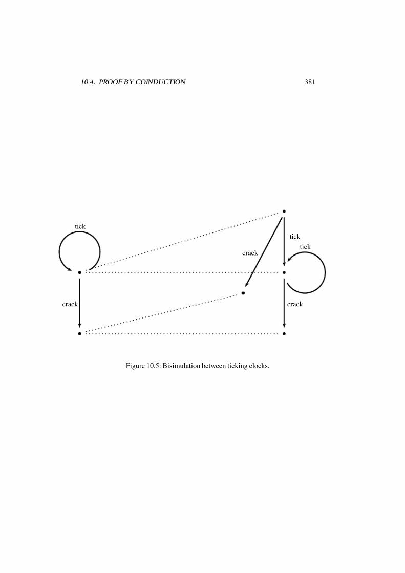
7/16/2019 The Haskell Road to Logic Maths and Programming
http://slidepdf.com/reader/full/the-haskell-road-to-logic-maths-and-programming-5634fa29ef7e9 392/448
10.4. PROOF BY COINDUCTION 381
crack
crack
crack
tick
tick
tick
Figure 10.5: Bisimulation between ticking clocks.

7/16/2019 The Haskell Road to Logic Maths and Programming
http://slidepdf.com/reader/full/the-haskell-road-to-logic-maths-and-programming-5634fa29ef7e9 393/448
382 CHAPTER 10. CORECURSION
Use
∼for the greatest bisimulation on a given set A (Exercise 10.27). Call two
elements of A bisimilar when they are related by a bisimulation on A. Beingbisimilar then coincides with being related by the greatest bisimulation:
a ∼ b ⇔ ∃R(R is a bisimulation, and aRb).
To show that two infinite objects x and y are equal, we show that they exhibit
the same behaviour, i.e. we show that x ∼ y. Such a proof is called a proof by
coinduction.
In the particular case of comparing streams we can make the notion of a bisimula-
tion more specific. There are only two kinds of observations on a stream: observ-
ing its head and observing its tail. Comparison of the heads should exhibit objects
that are the same. Comparison of the tails should exhibit bisimilar streams.
When talking about streams f = [f 0, f 1, f 2, f 3, . . .] it is convenient to refer to thetail of the stream as f . Thus, a stream f = [f 0, f 1, f 2, f 3, . . .] always has the form
f = f 0 : f , where f 0 is the head and f is the tail.
f 0f f
Figure 10.6: A stream viewed as a transition system.
f
f 0
f ¡
¡ g
g0
g¢
¢
¢
¢
Figure 10.7: Bisimulation between streams.
Viewing a stream f as a transition system, we get transitions f f 0−→ f , and so
on (Figure 10.6). A bisimulation between streams f and g that connects f and

7/16/2019 The Haskell Road to Logic Maths and Programming
http://slidepdf.com/reader/full/the-haskell-road-to-logic-maths-and-programming-5634fa29ef7e9 394/448
10.4. PROOF BY COINDUCTION 383
g is given in Figure 10.7. It is immediate from the picture that the notion of a
bisimulation between streams boils down to the following.
A stream bisimulation on a set A is a relation R on [A] with the following prop-
erty. If f, g ∈ [A] and f Rg then both f 0 = g0 and f Rg.
The general pattern of a proof by coinduction using stream bisimulations of f ∼ g,
where f, g ∈ [A], is simply this. Define a relation R on [A]. Next, show that R is
a stream bisimulation, with f Rg.
Example 10.29 As an example, we will show:
map f (iterate f x) ∼ iterate f (f x).
Let R be the following relation on [A].
(map f (iterate f x), iterate f (f x)) | f :: a → a, x :: a.
Suppose:
(map f (iterate f x)) R (iterate f (f x)).
We show that R is a bisimulation. We have:
map f (iterate f x)iterate
= map f x : (iterate f (f x))map= (f x) : map f (iterate f (f x))
iterate f (f x)iterate
= (f x) : iterate f (f (f x)).
This shows:
map f (iterate f x)head−→ (f x) (1)
map f (iterate f x)tail−→ map f x : (iterate f (f x)) (2)
iterate f (f x)head−→ (f x) (3)
iterate f (f x)tail−→ iterate f (f (f x)) (4)
Clearly, map f (iterate f x) and iterate f (f x) have the same heads, and also,
their tails are R-related. This shows that R is a bisimimulation that connects
map f (iterate f x) and iterate f (f x). Hence
(map f (iterate f x)) ∼ (iterate f (f x)).

7/16/2019 The Haskell Road to Logic Maths and Programming
http://slidepdf.com/reader/full/the-haskell-road-to-logic-maths-and-programming-5634fa29ef7e9 395/448
384 CHAPTER 10. CORECURSION
Given: A labeled transition system (Q,A,T ) . . .
To be proved: q ∼ p
Proof:
Let R be given by . . . and suppose qRp.
To be proved: R is a bisimulation.
Suppose q a−→ q
To be proved: There is a p ∈ Q with pa−→ p and q Rp.
Proof: . . .
Suppose pa
−→ p
To be proved: There is a q ∈ Q with q a−→ q and q Rp.Proof: . . .
Thus R is a bisimulation with qRp.
Thus q ∼ p.
Given: . . .
To be proved: f ∼ g
Proof:
Let R be given by . . . and suppose f Rg.
To be proved: R is a stream bisimulation.
To be proved: f 0 = g0.
Proof: . . .
To be proved: f Rg.
Proof: . . .
Thus R is a stream bisimulation with f Rg.
Thus f ∼ g.
Figure 10.8: Proof Recipes for Proofs by Coinduction.

7/16/2019 The Haskell Road to Logic Maths and Programming
http://slidepdf.com/reader/full/the-haskell-road-to-logic-maths-and-programming-5634fa29ef7e9 396/448
10.5. POWER SERIES AND GENERATING FUNCTIONS 385
Exercise 10.30 Show by means of a coinduction argument that for every infinite
list xs :: [a], every f : : a - > b, and every total predicate p :: b -> Boolthe following holds:
filter p (map f xs) = map f (filter ( p.f ) xs).
10.5 Power Series and Generating Functions
module PowerSeries
where
import Polynomials
instance Fractional a => Fractional [a] where
fromRational c = [fromRational c]
fs / [] = error "division by 0 attempted"
[] / gs = []
(0:fs) / (0:gs) = fs / gs
(_:fs) / (0:gs) = error "division by 0 attempted"
(f:fs) / (g:gs) = let q = f/g in
q : (fs - q.*gs) / (g:gs)
int :: Fractional a => [a] -> [a]
int fs = 0 : int1 fs 1 where
int1 [] _ = []
int1 (g:gs) n = g/n : (int1 gs (n+1))
expz = 1 + (int expz)
Figure 10.9: A Module for Power Series.
In chapter 9 we have seen how polynomials can get represented as finite lists of
their coefficients, and how operations on polynomials can be given directly on
these list representations. We will now generalize this to infinite sequences. A
7/16/2019 The Haskell Road to Logic Maths and Programming
http://slidepdf.com/reader/full/the-haskell-road-to-logic-maths-and-programming-5634fa29ef7e9 397/448
386 CHAPTER 10. CORECURSION
possible motivation for this (one of many) is the wish to define a division operation
on polynomials.
Suppose we want to divide
f (z) = f 0 + f 1z + f 2z2 + · · · + f kzk
by
g(z) = g0 + g1z + g2z2 + · · · + gmzm.
The outcome h(z) = h0 + h1z + h2z2 + · · · has to satisfy:
f (z) = h(z) · g(z).
This gives:
f 0 + zf (z) = (h0 + zh(z))g(z)
= h0g(z) + zh(z)g(z)= h0(g0 + zg(z)) + zh(z)g(z)
= h0g0 + z(h0g(z) + h(z)g(z)).
Thus, f 0 = h0g0, hence h0 = f 0g0
, and f (z) = h0g(z) + h(z)g(z), so from this
h(z) =f (z)−h0g(z)
g(z) . We see from this that computing fractions can be done by a
process of long division:
f (z)
g(z)=
f 0g0
+ zf (z) − (f 0/g0)g(z)
g(z). (div)
An example case is 11−z . Long division gives:
1
1 − z
=1 − z
1 − z
+ z1
1 − z
= 1 + z1
1 − z= 1 + z(1 + z
1
1 − z) = 1 + z(1 + z(1 + z
1
1 − z)) = · · ·
The representation of 1 − z is [1, −1], so in terms of computation on sequences we
get:
[1]
[1, −1]=
1
1:
[1]
[1, −1]
=1
1:
1
1:
[1]
[1, −1]
=1
1:
1
1:
1
1:
[1]
[1, −1]
=1
1 :1
1 :1
1 :1
1 :[1]
[1, −1]= . . .
7/16/2019 The Haskell Road to Logic Maths and Programming
http://slidepdf.com/reader/full/the-haskell-road-to-logic-maths-and-programming-5634fa29ef7e9 398/448
10.5. POWER SERIES AND GENERATING FUNCTIONS 387
This shows that 11−z
does not have finite degree. It is not a polynomial.
To get at a class of functions closed under division we define power series to be
functions of the form
f (z) = f 0 + f 1z + f 2z2 + · · · =
∞k=0
f kzk.
A power series is represented by an infinite stream [f 0, f 1, f 2, . . .]. Power series in
a variable z can in fact be viewed as approximations to complex numbers (Section
8.10), but we will not pursue that connection here.
The implementation of division follows the formula (div). Since trailing zeros
are suppressed, we have to take the fact into account that [] represents an infinite
stream of zeros.
fs / [] = error "division by 0 attempted"
[] / gs = []
(0:fs) / (0:gs) = fs / gs
(_:fs) / (0:gs) = error "division by 0 attempted"
(f:fs) / (g:gs) = let q = f/g in q : (fs - q.*gs)/(g:gs)
Here are some Haskell computations involving division:
COR> take 10 (1/(1-z))
[1 % 1,1 % 1,1 % 1,1 % 1,1 % 1,1 % 1,1 % 1,1 % 1,1 % 1,1 % 1]
COR> take 10 (1/(1+z))
[1 % 1,-1 % 1,1 % 1,-1 % 1,1 % 1,-1 % 1,1 % 1,-1 % 1,1 % 1,-1 % 1]
Example 10.31 To get a feel for ‘long division with sequences’, we compute 33−z ,
as a calculation on sequences. The sequence representation of 3 − z is [3, −1], so
we get:
[3]
[3, −1]=
3
3:
[1]
[3, −1]
=3
3:
1
3:
[1/3]
[3, −1]
=3
3:
1
3:
1
9:
[1/9]
[3, −1]
=3
3 :1
3 :1
9 :1
27 :[1/27]
[3, −1]= . . .

7/16/2019 The Haskell Road to Logic Maths and Programming
http://slidepdf.com/reader/full/the-haskell-road-to-logic-maths-and-programming-5634fa29ef7e9 399/448
388 CHAPTER 10. CORECURSION
This is indeed what Haskell calculates for us:
COR> take 9 (3 /(3-z))
[1 % 1,1 % 3,1 % 9,1 % 27,1 % 81,1 % 243,1 % 729,1 % 2187,1 % 6561]
Integration involves division, for z
0f (t)dt is given by
0 + f 0z +1
2f 1z2 +
1
3f 2z3 + · · ·
To give an example, if g(z) = 11−z , then
z0
g(t)dt equals:
0 + z +1
2
z2 +1
3
z3 +
· · ·Integration is implemented by:
int :: Fractional a => [a] -> [a]
int [] = []
int fs = 0 : int1 fs 1 where
int1 [] _ = []
int1 (g:gs) n = g/n : (int1 gs (n+1))
We get:
COR> take 10 (int (1/(1-z)))[0 % 1,1 % 1,1 % 2,1 % 3,1 % 4,1 % 5,1 % 6,1 % 7,1 % 8,1 % 9]
To extend composition to power series, we have to be careful, for the equation
f (g(z)) = f 0 + g(z) · f (g(z)) has a snag: the first coefficient depends on all of f ,which is a problem if f is a power series. Here is an example:
COR> comp1 ones [0,2] where ones = 1 : ones
ERROR - Garbage collection fails to reclaim sufficient space
To solve this, we must develop the equation for composition a bit further:
f (g(z)) = f 0 + g(z)
·f (g(z))
= f 0 + (g0 + zg(z)) · f (g(z))
= (f 0 + g0 · f (g(z))) + zg(z) · f (g(z))

7/16/2019 The Haskell Road to Logic Maths and Programming
http://slidepdf.com/reader/full/the-haskell-road-to-logic-maths-and-programming-5634fa29ef7e9 400/448
10.5. POWER SERIES AND GENERATING FUNCTIONS 389
In the special case where g0 = 0 we can simplify this further:
f (zg(z)) = f 0 + zg(z) · f (zg(z)).
This leads immediately to the following implementation (part of the module for
Polynomials):
comp :: Num a => [a] -> [a] -> [a]
comp _ [] = error ".."
comp [] _ = []
comp (f:fs) (0:gs) = f : gs * (comp fs (0:gs))
comp (f:fs) (g:gs) = ([f] + [g] * (comp fs (g:gs)))
+ (0 : gs * (comp fs (g:gs)))
This gives:
COR> take 15 (comp ones [0,2]) where ones = 1 : ones
[1,2,4,8,16,32,64,128,256,512,1024,2048,4096,8192,16384]
Figure 10.9 gives a module for power series. We will now show how this is can
be used as a tool for combinatorial calculations. We are interested in finite lists
[f 0, . . . , f n] or infinite lists [f 0, f 1, f 2, . . .] that can be viewed as solutions to com-
binatorial problems.
We associate sequences with combinatorial problems by saying that [f 0, f 1, f 2, . . .]
solves a combinatorial problem if f r gives the number of solutions for that prob-lem (cf. the use of polynomials for solving combinatorial problems in section 9.4,
which is now generalized to power series).
We call a power series f (z) a generating function for a combinatorial problem
if the list of coefficients of f (z) solves that problem. If f (z) has power series
expansion f 0 + f 1z + f 2z2 + f 3z3 + · · · , then f (z) is a generating function for
[f 0, f 1, f 2, f 3, . . .].
Example 10.32 Find a generating function for [1, 1, 1, 1, . . .]. Solution: as we saw
above 11−z has power series expansion 1 + z + z2 + z3 + z4 + · · · . The list of
coefficients is [1, 1, 1, 1, . . .].
The generating function 1
1−zis an important building block for constructing other
generating functions, so we should give it a name. In fact, we already did: ones
names the list [1,1,1,1,..]. As long as we don’t use division, this is OK.
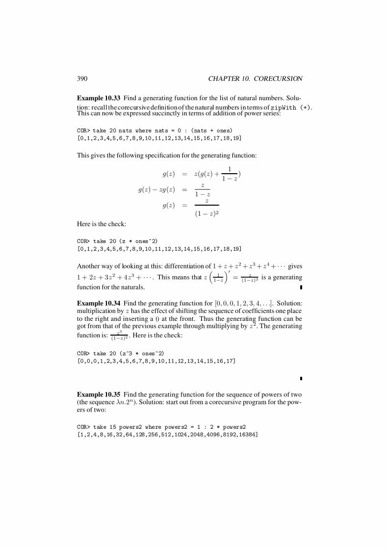
7/16/2019 The Haskell Road to Logic Maths and Programming
http://slidepdf.com/reader/full/the-haskell-road-to-logic-maths-and-programming-5634fa29ef7e9 401/448
390 CHAPTER 10. CORECURSION
Example 10.33 Find a generating function for the list of natural numbers. Solu-
tion: recall the corecursive definition of the natural numbers in terms of zipWith (+).This can now be expressed succinctly in terms of addition of power series:
COR> take 20 nats where nats = 0 : (nats + ones)
[0,1,2,3,4,5,6,7,8,9,10,11,12,13,14,15,16,17,18,19]
This gives the following specification for the generating function:
g(z) = z(g(z) +1
1 − z)
g(z) − zg(z) =z
1 − z
g(z) =z
(1 − z)2
Here is the check:
COR> take 20 (z * ones^2)
[0,1,2,3,4,5,6,7,8,9,10,11,12,13,14,15,16,17,18,19]
Another way of looking at this: differentiation of 1 + z + z2 + z3 + z4 + · · · gives
1 + 2z + 3z2 + 4z3 + · · · . This means that z
11−z
= z
(1−z)2 is a generating
function for the naturals.
Example 10.34 Find the generating function for [0, 0, 0, 1, 2, 3, 4, . . .]. Solution:multiplication by z has the effect of shifting the sequence of coefficients one place
to the right and inserting a 0 at the front. Thus the generating function can begot from that of the previous example through multiplying by z2. The generating
function is: z3
(1−z)2 . Here is the check:
COR> take 20 (z 3 * ones^2)
[0,0,0,1,2,3,4,5,6,7,8,9,10,11,12,13,14,15,16,17]
Example 10.35 Find the generating function for the sequence of powers of two(the sequence λn.2n). Solution: start out from a corecursive program for the pow-ers of two:
COR> take 15 powers2 where powers2 = 1 : 2 * powers2
[1,2,4,8,16,32,64,128,256,512,1024,2048,4096,8192,16384]

7/16/2019 The Haskell Road to Logic Maths and Programming
http://slidepdf.com/reader/full/the-haskell-road-to-logic-maths-and-programming-5634fa29ef7e9 402/448
10.5. POWER SERIES AND GENERATING FUNCTIONS 391
This immediately leads to the specification g(z) = 1 + 2zg(z) (the factor z shifts
one place to the right, the summand 1 puts 1 in first position). It follows thatg(z) = 1
1−2z . Here is the confirmation:
COR> take 10 (1/(1-2*z))
[1 % 1,2 % 1,4 % 1,8 % 1,16 % 1,32 % 1,64 % 1,128 % 1,256 % 1,512 % 1]
Example 10.36 If g(z) is the generating function for λn.gn, then λn.gn+1 is gen-
erated byg(z)z
, for multiplication by 1z
shifts the coefficients of the power series
one place to the left. Thus, the generating function for the sequence λn.n + 1 is1
(1−z)2 . This sequence can also be got by adding the sequence of naturals and the
sequence of ones, i.e., it is also generated by z
(1−z)2 + 1
1−z. This identification
makes algebraic sense:
z
(1 − z)2+
1
1 − z=
z
(1 − z)2+
1 − z
(1 − z)2=
1
(1 − z)2.
Exercise 10.37 Find the generating functions for
[0, 0, 0, 1, 1, 1, . . .],
for
[1, 1, 1, 0, 0, 0, . . .],
and for[1,
12
,14
,18
, . . .].
Check your answers by computer.
Example 10.38 Find the generating function for [0, 1, 0, 1, 0, 1, . . .]. Solution: thesequence is generated by the following corecursive program.
COR> take 20 things where things = 0 : 1 : things
[0,1,0,1,0,1,0,1,0,1,0,1,0,1,0,1,0,1,0,1]
This leads to the specification g(z) = 0 + z(1 + zg(z)), which reduces to g(z) =z + z2g(z). From this, g(z) = z
1−z2 . In a similar way we can derive the generat-
ing function for [1, 0, 1, 0, 1, 0, . . .], which turns out to be g(z) = 1
1−z2 . Alterna-
tively, observe that [1, 0, 1, 0, 1, 0, . . .] is the result of shifting [0, 1, 0, 1, 0, 1, . . .]one place to the left, so division by z does the trick.

7/16/2019 The Haskell Road to Logic Maths and Programming
http://slidepdf.com/reader/full/the-haskell-road-to-logic-maths-and-programming-5634fa29ef7e9 403/448
392 CHAPTER 10. CORECURSION
Theorem 10.39 summarizes a number of recipes for finding generating functions.
Theorem 10.39 Suppose f (z) is a generating function for λn.f n and g(z) is the
generating function for λn.gn. Then:
1. c1−z is the generating function for λn.c.
2. z(1−z)2 is the generating function for λn.n.
3.f (z)z
is the generating function for λn.f n+1.
4. cf (z) + dg(z) is the generating function for λn.cf n + dgn.
5. (1 − z)f (z) is the generating function for the difference sequence
λn.f n − f n−1.6. 1−z
zf (z) is the generating function for the difference sequence
λn.f n+1 − f n.
7. 11−zf (z) is the generating function for λn.f 0 + f 1 + · · · + f n.
8. f (z)g(z) is the generating function for λn.f 0gn+ f 1gn−1 + · · ·+ f n−1g1 +f ng0 (the convolution of f and g).
9. zf (z) is the generating function for λn.nf n.
10. 1z
z0
f (t)dt is the generating function for λn. f nn+1 .
Exercise 10.40 Prove the statements of theorem 10.39 that were not proved in the
examples.
Example 10.41 Find the generating function for the sequence λn.2n + 1. Solu-tion: the odd natural numbers are generated by the following corecursive program:
COR> take 20 (ones + 2 * nats)
[1,3,5,7,9,11,13,15,17,19,21,23,25,27,29,31,33,35,37,39]
This immediately gives g(z) = 11−z + 2
(1−z)2 .
Example 10.42 Find the generating function for the sequence λn.(n + 1) 2. So-
lution: the generating function is the sum of the generating functions for λn.n2,
λn.2n and λn.1. One way to proceed would be to find these generating functions
and take their sum. But there is an easier method. Recall that (n + 1)2 is the sum
of the first n odd numbers, and use the recipe from Theorem 10.39 for forming

7/16/2019 The Haskell Road to Logic Maths and Programming
http://slidepdf.com/reader/full/the-haskell-road-to-logic-maths-and-programming-5634fa29ef7e9 404/448
10.5. POWER SERIES AND GENERATING FUNCTIONS 393
the sequence λn.a0 +
· · ·+ an, by means of dividing the generating function from
Example 10.41 by 1 − z. This immediately gives 1(1−z)2 + 2z
(1−z)3 .
Alternatively, Theorem 10.39 tells us that λn.(n + 1)2 can also be defined fromthe naturals with the help of differentiation:
COR> take 20 (deriv nats)
[1,4,9,16,25,36,49,64,81,100,121,144,169,196,225,256,289,324,361,400]
It follows that the generating function g(z), for g(z) should satisfy:
g(z) =
z
(1 − z)2
.
Working this out we find that g(z) =1
(1−z)2 +2z
(1−z)3 .
Finally, here is computational confirmation:
COR> take 20 (ones^2 + 2 * z * ones^3)
[1,4,9,16,25,36,49,64,81,100,121,144,169,196,225,256,289,324,361,400]
Example 10.43 Find the generating function for λn.n2. Solution: shift the solu-tion for the previous example to the right by multiplication by z. This gives:
COR> take 20 (z * ones^2 + 2 * z^2 * ones^3)
[0,1,4,9,16,25,36,49,64,81,100,121,144,169,196,225,256,289,324,361]
So the generating function is g(z) = z(1−z)2 + 2z2
(1−z)3 . Sure enough, we can also
get the desired sequence from the naturals by shift and differentiation:
COR> take 20 (z * deriv nats)
[0,1,4,9,16,25,36,49,64,81,100,121,144,169,196,225,256,289,324,361]
Example 10.44 Find the generating function for the sequence of Fibonacci num-bers. Solution: consider again the corecursive definition of the Fibonacci numbers.We can express this succinctly in terms of addition of power series, as follows:
COR> take 20 fibs where fibs = 0 : 1 : (fibs + (tail fibs))
[0,1,1,2,3,5,8,13,21,34,55,89,144,233,377,610,987,1597,2584,4181]

7/16/2019 The Haskell Road to Logic Maths and Programming
http://slidepdf.com/reader/full/the-haskell-road-to-logic-maths-and-programming-5634fa29ef7e9 405/448
394 CHAPTER 10. CORECURSION
This is easily translated into an instruction for a generating function:
g(z) = z2
g(z) +
g(z)
z
+ z.
Explanation: multiplying by z2 inserts two 0’s in front of the fibs sequence, and
adding z changes the second of these to 1 (the meaning is: the second coefficient
is obtained by add 1 to the previous coefficient).g(z)z
gives the tail of the fibs
sequence. From this we get:
g(z) − zg(z) − z2g(z) = z
g(z) =z
1 − z − z2
And lo and behold:
COR> take 10 (z/(1-z-z^2))
[0 % 1,1 % 1,1 % 1,2 % 1,3 % 1,5 % 1,8 % 1,13 % 1,21 % 1,34 % 1]
Exercise 10.45 The Lucas numbers are given by the following recursion:
L0 = 2, L1 = 1, Ln+2 = Ln + Ln+1.
This gives:
[2, 1, 3, 4, 7, 11, 18, 29, 47, 76, 123, 199, 322, 521, 843, 1364, 2207, 3571, . . .]
The recipe is that for the Fibonacci numbers, but the initial element of the list is 2instead of 0. Find a generating function for the Lucas numbers, starting out from
an appropriate corecursive definition.
Example 10.46 Recall the definition of the Catalan numbers from Exercise 7.20:
C 0 = 1, C n+1 = C 0C n + C 1C n−1 + · · · + C n−1C 1 + C nC 0.
Clearly, C n+1 is obtained from [C 0, . . . , C n] by convolution of that list with itself.This leads to the following corecursive definition of the Catalan numbers:
COR> take 15 cats where cats = 1 : cats * cats
[1,1,2,5,14,42,132,429,1430,4862,16796,58786,208012,742900,2674440]
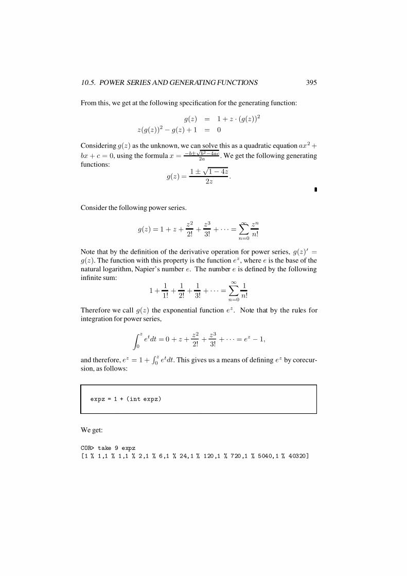
7/16/2019 The Haskell Road to Logic Maths and Programming
http://slidepdf.com/reader/full/the-haskell-road-to-logic-maths-and-programming-5634fa29ef7e9 406/448
10.5. POWER SERIES AND GENERATING FUNCTIONS 395
From this, we get at the following specification for the generating function:
g(z) = 1 + z · (g(z))2
z(g(z))2 − g(z) + 1 = 0
Considering g(z) as the unknown, we can solve this as a quadratic equation ax2 +
bx + c = 0, using the formula x = −b±√ b2−4ac2a . We get the following generating
functions:
g(z) =1 ± √
1 − 4z
2z.
Consider the following power series.
g(z) = 1 + z +z2
2!+
z3
3!+ · · · =
∞n=0
zn
n!
Note that by the definition of the derivative operation for power series, g(z) =g(z). The function with this property is the function ez , where e is the base of the
natural logarithm, Napier’s number e. The number e is defined by the following
infinite sum:
1 +1
1!+
1
2!+
1
3!+ · · · =
∞n=0
1
n!
Therefore we call g(z) the exponential function ez . Note that by the rules for
integration for power series,
z0
etdt = 0 + z +z2
2!+
z3
3!+ · · · = ez − 1,
and therefore, ez = 1 + z
0etdt. This gives us a means of defining ez by corecur-
sion, as follows:
expz = 1 + (int expz)
We get:
COR> take 9 expz
[1 % 1,1 % 1,1 % 2,1 % 6,1 % 24,1 % 120,1 % 720,1 % 5040,1 % 40320]
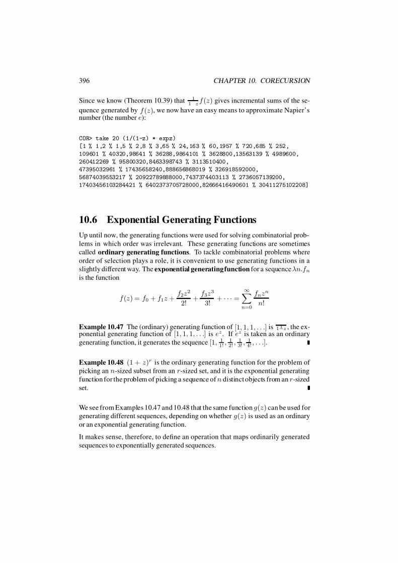
7/16/2019 The Haskell Road to Logic Maths and Programming
http://slidepdf.com/reader/full/the-haskell-road-to-logic-maths-and-programming-5634fa29ef7e9 407/448
396 CHAPTER 10. CORECURSION
Since we know (Theorem 10.39) that 11−z
f (z) gives incremental sums of the se-
quence generated by f (z), we now have an easy means to approximate Napier’snumber (the number e):
COR> take 20 (1/(1-z) * expz)
[1 % 1,2 % 1,5 % 2,8 % 3,65 % 24,163 % 60,1957 % 720,685 % 252,
109601 % 40320,98641 % 36288,9864101 % 3628800,13563139 % 4989600,
260412269 % 95800320,8463398743 % 3113510400,
47395032961 % 17435658240,888656868019 % 326918592000,
56874039553217 % 20922789888000,7437374403113 % 2736057139200,
17403456103284421 % 6402373705728000,82666416490601 % 30411275102208]
10.6 Exponential Generating Functions
Up until now, the generating functions were used for solving combinatorial prob-
lems in which order was irrelevant. These generating functions are sometimes
called ordinary generating functions. To tackle combinatorial problems where
order of selection plays a role, it is convenient to use generating functions in a
slightly different way. The exponential generating function for a sequence λn.f nis the function
f (z) = f 0 + f 1z +f 2z2
2!+
f 3z3
3!+ · · · =
∞n=0
f nzn
n!
Example 10.47 The (ordinary) generating function of [1, 1, 1, . . .] is 11−z , the ex-ponential generating function of [1, 1, 1, . . .] is ez . If ez is taken as an ordinary
generating function, it generates the sequence [1, 11! , 1
2! , 13! , 1
4! , . . .].
Example 10.48 (1 + z)r is the ordinary generating function for the problem of
picking an n-sized subset from an r-sized set, and it is the exponential generating
function for the problem of picking a sequence of n distinct objects from an r-sized
set.
We see from Examples 10.47 and 10.48 that the same function g(z) can be used for
generating different sequences, depending on whether g(z) is used as an ordinary
or an exponential generating function.
It makes sense, therefore, to define an operation that maps ordinarily generated
sequences to exponentially generated sequences.

7/16/2019 The Haskell Road to Logic Maths and Programming
http://slidepdf.com/reader/full/the-haskell-road-to-logic-maths-and-programming-5634fa29ef7e9 408/448
10.6. EXPONENTIAL GENERATING FUNCTIONS 397
o2e :: Num a => [a] -> [a]o2e [] = []
o2e (f:fs) = f : o2e (deriv (f:fs))
With this we get:
COR> take 10 (o2e expz)
[1 % 1,1 % 1,1 % 1,1 % 1,1 % 1,1 % 1,1 % 1,1 % 1,1 % 1,1 % 1]
A function for converting from exponentially generated sequences to ordinarily
generated sequences is the converse of this, so it uses integration:
e2o :: Fractional a => [a] -> [a]
e2o [] = []
e2o (f:fs) = [f] + (int (e2o (fs)))
This gives:
COR> take 9 (e2o (1/(1-z)))
[1 % 1,1 % 1,1 % 2,1 % 6,1 % 24,1 % 120,1 % 720,1 % 5040,1 % 40320]
Example 10.49 Here is how (z + 1)10
is used to solve the problem of finding thenumber of ways of picking subsets from a set of 10 elements:
COR> (1+z)^10
[1,10,45,120,210,252,210,120,45,10,1]
And here is how the same function is used to solve the problem of finding thenumber of ways to pick sequences from a set of 10 elements:
COR> o2e ((1+z)^10)
[1,10,90,720,5040,30240,151200,604800,1814400,3628800,3628800]
Example 10.50 Suppose a vase contains red, white and blue marbles, at least fourof each kind. How many ways are there of arranging sequences of marbles from

7/16/2019 The Haskell Road to Logic Maths and Programming
http://slidepdf.com/reader/full/the-haskell-road-to-logic-maths-and-programming-5634fa29ef7e9 409/448
398 CHAPTER 10. CORECURSION
the vase, with at most four marbles of the same colour? Solution: the exponential
generating function is (1 + z + z22 + z3
6 + z424 )3. The idea: if you pick n marbles of
the same colour, then n! of the marble orderings become indistinguishable. Hereis the Haskell computation of the solution.
COR> o2e ([1,1,1/2,1/6,1/24]^3)
[1 % 1,3 % 1,9 % 1,27 % 1,81 % 1,240 % 1,690 % 1,1890 % 1,4830 % 1,
11130 % 1,22050 % 1,34650 % 1,34650 % 1]
Example 10.51 Suppose a vase contains red, white and blue marbles, an unlim-ited supply of each colour. How many ways are there of arranging sequences of marbles from the vase, assume that at least two marbles are of the same colour?
Solution: a suitable exponential generating function is (ez−z −1)3 = ( z2
2 + z3
6 +z4
24 + · · · )3:
COR> take 10 (o2e ((expz - z - 1)^3))
[0 % 1,0 % 1,0 % 1,0 % 1,0 % 1,0 % 1,90 % 1,630 % 1,2940 % 1,11508 % 1]
This gives the number of solutions for up to 9 marbles. For up to 5 marbles there
are no solutions. There are 90 = 6!23 sequences containing two marbles of each
colour. And so on.
Exercise 10.52 Suppose a vase contains red, white and blue marbles, at least four
of each kind. How many ways are there of arranging sequences of marbles from
the vase, with at least two and at most four marbles of the same colour?
10.7 Further Reading
Domain theory and proof by approximation receive fuller treatment in [DP02].
Generating functions are a main focus in [GKP89]. The connection between gen-
erating functions and lazy semantics is the topic of [Kar97, McI99, McI00]. A
coinductive calculus of streams and power series is presented in [Rut00]. Core-
cursion is intimately connected with circularity in definitions [BM96] and with the
theory of processes and process communication [Fok00, Mil99].

7/16/2019 The Haskell Road to Logic Maths and Programming
http://slidepdf.com/reader/full/the-haskell-road-to-logic-maths-and-programming-5634fa29ef7e9 410/448
Chapter 11
Finite and Infi nite Sets
Preview
Some sets are bigger than others. For instance, finite sets such as ∅ and 0, 1, 2,
are smaller than infinite ones such as N and R. But there are varieties of infinity:
the infinite set R is bigger than the infinite set N, in a sense to be made precise in
this chapter.
This final chapter starts with a further discussion of the Principle of Mathematical
Induction as the main instrument to fathom the infinite with, and explains why
some infinite sets are incomparably larger than some others.
module FAIS
where
11.1 More on Mathematical Induction
The natural numbers form the set N =
0, 1, 2, . . .
. The Principle of Mathemati-
cal Induction allows you to prove universal statements about the natural numbers,
that is, statements of the form ∀n ∈ N E (n).
399

7/16/2019 The Haskell Road to Logic Maths and Programming
http://slidepdf.com/reader/full/the-haskell-road-to-logic-maths-and-programming-5634fa29ef7e9 411/448
400 CHAPTER 11. FINITE AND INFINITE SETS
Fact 11.1 (Mathematical Induction) For every set X
⊆N , we have that:
if 0 ∈ X and ∀n∈N(n ∈ X ⇒ n + 1 ∈ X ) , then X = N.
This looks not impressive at all, since it is so obviously true. For, suppose that
X ⊆ N satisfies both 0 ∈ X and ∀n ∈ N(n ∈ X ⇒ n + 1 ∈ X ). Then
we see that N ⊆ X (and, hence, that X = N) as follows. First, we have as a
first Given, that 0 ∈ X . Then the second Given (∀-elimination, n = 0) yields
that 0 ∈ X ⇒ 1 ∈ X . Therefore, 1 ∈ X . Applying the second Given again
(∀-elimination, n = 1) we obtain 1 ∈ X ⇒ 2 ∈ X ; therefore, 2 ∈ X . And so
on, for all natural numbers.
Nevertheless, despite its being so overly true, it is difficult to overestimate the
importance of induction. It is essentially the only means by with we acquire infor-
mation about the members of the infinite setN
.
Sets versus Properties. With every property E of natural numbers there corre-
sponds a set n ∈ N | E (n) of natural numbers. Thus, induction can also be
formulated using properties instead of sets. It then looks as follows:
If E is a property of natural numbers such that
(i) E (0),
(ii) ∀n∈N [E (n) ⇒ E (n + 1)],
then ∀n∈N E (n).
Induction: Basis, Step, Hypothesis. According to Induction, in order that E (n)is true for all n ∈ N, it suffices that
(i) this holds for n = 0, i.e., E (0) is true, and
(ii) this holds for a number n + 1, provided it holds for n.
As we have seen, the proof of (i) is called basis of a proof by induction, the proof
of (ii) is called the induction step. By the introduction rules for ∀ and ⇒, in order
to carry out the induction step, you are granted the Given E (n) for an arbitrary
number n, whereas you have to show that E (n + 1). The assumption that E (n) is
called the induction hypothesis. The nice thing about induction is that this induc-
tion hypothesis comes entirely free.
Fact 11.2 (Scheme for Inductions) Viewed as a rule of proof, induction can be
schematized as follows.

7/16/2019 The Haskell Road to Logic Maths and Programming
http://slidepdf.com/reader/full/the-haskell-road-to-logic-maths-and-programming-5634fa29ef7e9 412/448
11.1. MORE ON MATHEMATICAL INDUCTION 401
E (n)
...
E (0) E (n + 1)∀nE (n)
A proof using the Principle of Induction of a statement of the form ∀n E (n) is
called a proof with induction with respect to n. It can be useful to mention the
parameter n when other natural numbers surface in the property E .
According to the above schema, the conclusion ∀n E (n) can be drawn on the basis
of (i) the premiss that E (0), and (ii) a proof deriving E (n + 1) on the basis of the
induction hypothesis E (n).
The following strong variant of induction is able to perform tasks that are beyondthe reach of the ordinary version. This time, we formulate the principle in terms
of properties.
Fact 11.3 (Strong Induction) For every property E of natural numbers:
if ∀n∈N [ (∀m < n E (m)) ⇒ E (n) ] , then ∀n∈NE (n).
Using strong induction, the condition ∀m< n E (m) acts as the induction hypoth-
esis from which you have to derive that E (n).
This is (at least, for n > 1) stronger than in the ordinary form. Here, to establish
that E (n), you are given that E (m) holds for all m < n. In ordinary induction,
you are required to show that E (n + 1) on the basis of the Given that it holds for
n only.
Note: using ordinary induction you have to accomplish two things: basis, and
induction step. Using strong induction, just one thing suffices. Strong induction
has no basis.
Proof. (of 11.3.) Suppose that ∀n∈N [ (∀m < n E (m)) ⇒ E (n) ]. (1)
Define the set X by X = n | ∀m < n E (m). Assumption (1) says that every
element of X has property E . Therefore, it suffices showing that every natural
number is in X . For this, we employ ordinary induction.
Basis. 0 ∈ X .I.e.: ∀m < 0 E (m); written differently: ∀m[m < 0 ⇒ E (m)]. This holds trivially
since there are no natural numbers < 0. The implication m < 0⇒
E (m) is
trivially satisfied.
Induction step.

7/16/2019 The Haskell Road to Logic Maths and Programming
http://slidepdf.com/reader/full/the-haskell-road-to-logic-maths-and-programming-5634fa29ef7e9 413/448
402 CHAPTER 11. FINITE AND INFINITE SETS
Assume that (induction hypothesis) n
∈X . That means:
∀m < n E (m). As-
sumption (1) implies, that E (n) is true. Combined with the induction hypothesis,we obtain that ∀m < n + 1 E (m). This means, that n + 1 ∈ X . The induction
step is completed.
Induction now implies, that X = N. According to the remark above, we have that
∀n∈N E (n).
It is useful to compare the proof schemes for induction and strong induction. Here
they are, side by side:
E (n)...
E (0) E (n + 1)
∀nE (n)
∀m < n E (m)...
E (n)
∀nE (n)
An alternative to strong induction that is often used is the minimality principle.
Fact 11.4 (Minimality Principle) Every non-empty set of natural numbers has a
least element.
Proof. Assume that A is an arbitrary set of natural numbers. It clearly suffices to
show that, for each n ∈ N,
n ∈ A ⇒ A has a least element.
For, if also is given that A
=
∅, then some n
∈A must exist. Thus the implication
applied to such an element yields the required conclusion.
Here follows a proof of the statement using strong induction w.r.t. n. Thus, assume
that n is an arbitrary number for which:
Induction hypothesis: for every m < n: m ∈ A ⇒ A has a least element.
To be proved: n ∈ A ⇒ A has a least element.
Proof: Assume that n ∈ A. There are two cases.
(i) n is (by coincidence) the least element of A. Thus, A has a least element.
(ii) n is not least element of A. Then some m ∈ A exists such that m < n . So we
can apply the induction hypothesis and again find that A has a least element.
Remark. The more usual proof follows the logic from Chapter 2. This is much
more complicated, but has the advantage of showing the Minimality Principle to
be equivalent with Strong Induction.

7/16/2019 The Haskell Road to Logic Maths and Programming
http://slidepdf.com/reader/full/the-haskell-road-to-logic-maths-and-programming-5634fa29ef7e9 414/448
11.1. MORE ON MATHEMATICAL INDUCTION 403
Strong Induction is the following schema:
∀n[∀m < n E (m) ⇒ E (n)] ⇒ ∀n E (n).
Since E can be any property, it can also be a negative one. Thus:
∀n[∀m < n¬E (m) ⇒ ¬E (n)] ⇒ ∀n¬E (n).
The contrapositive of this is (Theorem 2.10 p. 45):
¬∀n¬E (n) ⇒ ¬∀n[∀m < n¬E (m) ⇒ ¬E (n)].
Applying Theorem 2.40 (p. 65):
∃n E (n) ⇒ ∃n¬[∀m < n¬E (m) ⇒ ¬E (n)].
Again Theorem 2.10:
∃n E (n) ⇒ ∃n[∀m < n¬E (m) ∧ ¬¬E (n)].
Some final transformations eventually yield:
∃n E (n) ⇒ ∃n[E (n) ∧ ¬∃m < n E (m)]
— which is Minimality formulated using properties.
Exercise 11.5 Prove Induction starting at m, that is: for every X ⊆ N, if m ∈ X and ∀n m(n ∈ X ⇒ n + 1 ∈ X ), then ∀n ∈ N(m n ⇒ n ∈ X ).
Hint. Apply induction to the set Y = n | m + n ∈ X .
Exercise 11.6 Suppose that X ⊆ N is such that 1 ∈ X and ∀n ∈ N(n ∈ X ⇒n + 2 ∈ X ). Show that every odd number is in X .
Definition 11.7 A relation ≺ on A is called well-founded if no infinite sequence
· · · ≺ a2 ≺ a1 ≺ a0 exists in A. Formulated differently: every sequence a0 a1 a2 · · · in A eventually terminates.
Example 11.8 According to Exercise 4.34 (p. 136), the relation ≺ on sets defined
by: a ≺ b iff ℘(a) = b, is well-founded.
An easier example is in the next exercise.
Exercise 11.9 Show that < is well-founded on N. That is: there is no infinite
sequence n0 > n1 > n2 > · · · .
Hint. Show, using strong induction w.r.t. n, that for all n∈N, E (n); where
E (n) signifies that no infinite sequence n0 = n > n1 > n2 > · · · starts at n.
Alternatively, use Exercise 11.10.

7/16/2019 The Haskell Road to Logic Maths and Programming
http://slidepdf.com/reader/full/the-haskell-road-to-logic-maths-and-programming-5634fa29ef7e9 415/448
404 CHAPTER 11. FINITE AND INFINITE SETS
Exercise 11.10* Well-foundedness as an induction principle. Let
≺be a rela-
tion on a set A.
1. Suppose that ≺ is well-founded. Assume that X ⊆ A satisfies
∀a ∈ A(∀b ≺ a(b ∈ X ) ⇒ a ∈ X ).
Show that X = A.
Hint. Show that any a0 ∈ A − X can be used to start an infinite sequence
a0 a1 a2 · · · in A.
2. Conversely:
Suppose that every X ⊆ A satisfying ∀a ∈ A(∀b ≺ a(b ∈ X ) ⇒ a ∈ X )
coincides with A. Show that ≺ is well-founded. Hint. Suppose that a0 a1 a2 · · · , and consider the set X = A −a0, a1, a2, . . ..
Exercise 11.11* Let R be a relationon a set A. Recall that R∗ denotes the reflexive
transitive closure of R, cf. Exercise 5.46 p. 173.
1. Assume that for all a, b1, b2 ∈ A, if aRb1 and aRb2, then c ∈ A exists such
that b1Rc and b2Rc.
Show that R is confluent , that is: for all a, b1, b2
∈A, if aR∗b1 and aR∗b2,
then c ∈ A exists such that b1R∗c and b2R∗c.
2. Assume that R is weakly confluent , that is: for all a, b1, b2 ∈ A, if aRb1 and
aRb2, then c ∈ A exists such that b1R∗c and b2R∗c.
A counter-example to confluence is called bad . That is: a is bad iff there
are b1, b2 ∈ A such that aR∗b1 and aR∗b2, and for no c ∈ A we have that
b1R∗c and b2R∗c.
Show: if a is bad, then a bad b exists such that aRb.
3. (In abstract term rewriting theory, the following result is known as New-
man’s Lemma.)
Assume that R is weakly confluent.
Furthermore, assume that R−1 is well-founded.
Show that R is confluent.

7/16/2019 The Haskell Road to Logic Maths and Programming
http://slidepdf.com/reader/full/the-haskell-road-to-logic-maths-and-programming-5634fa29ef7e9 416/448
11.1. MORE ON MATHEMATICAL INDUCTION 405
Hint. Use part 2; alternatively, use Exercise 11.10.
Remark. That R−1 is well-founded is necessary here.
For example, R = (1, 0), (1, 2), (2, 1), (2, 3) is weakly confluent but not
confluent.
Exercise 11.12 Suppose that∅ = X ⊆ N, and that X is bounded , i.e.: that m ∈ Nexists such that for all n ∈ X , n m. Show that X has a maximum, that is: an
element m ∈ X such that for all n ∈ X , n m.
Hint. Induction w.r.t. m. Thus, E (m) is: every non-empty X ⊆ N such that
∀n∈X (n m), has a maximum.
Exercise 11.13 Suppose that f : N → N is such that n < m ⇒ f (n) < f (m).Show by means of an induction argument that for all n ∈ N: n f (n).
Exercise 11.14 Suppose that a0, a1, a2, . . . is an infinite sequence of natural num-
bers. Prove that i, j ∈ N exist such that both i < j and ai aj.
Exercise 11.15 The function g : N+ × N+ → N+ has the following properties.
1. If n < m, then g(n, m) = g(n, m − n).
2. g(n, m) = g(m, n).
3. g(n, n) = n.
Show that g(n, m) is the gcd (greatest common divisor) of n and m.
Exercise 11.16* You play Smullyan’s ball game on your own. Before you is a
box containing finitely many balls. Every ball carries a natural number. Next to the
box, you have a supply of as many numbered balls as you possibly need. A move
in the game consists in replacing one of the balls in the box by arbitrarily (possibly
zero, but finitely) many new balls that carry a number smaller than that on the
one you replace. (Thus, 999 balls numbered 7 can replace one ball numbered 8,
but a ball numbered 0 can only be taken out of the box since there are no natural
numbers smaller than 0.)
Repeat this move.
Show that, no matter how you play the game, you’ll end up with an empty box
eventually. (Thus, your last moves necessarily consist in throwing away balls num-
bered 0.)

7/16/2019 The Haskell Road to Logic Maths and Programming
http://slidepdf.com/reader/full/the-haskell-road-to-logic-maths-and-programming-5634fa29ef7e9 417/448
406 CHAPTER 11. FINITE AND INFINITE SETS
Hint. Proof by Contradiction. Suppose that you can play ad infinitum, and that Bk
is how the box looks after your k-th move. Derive a contradiction applying stronginduction w.r.t. the greatest number n present on one of the balls in the box B0
you start from. If m is the number of balls in B0 carrying n, apply a second strong
induction, now w.r.t. m.
Exercise 11.17 Implement a simplified version of Smullyan’s ball game from theprevious exercise, where (i) the box of balls is represented as a list of integers, (ii)it is always the first integer n > 1 that gets replaced, (iii) an integer n > 1 getsreplaced by two copies of n − 1, (iv) the game terminates with a list consisting of just ones. The type declaration should run:
ballgame :: [Integer] -> [[Integer]].
How long will it take before ballgame [50] terminates? Minutes? Hours?Days? Years?
Exercise 11.18 The following theorem implies that, e.g., all inhabitants of Ams-
terdam have the same number of hairs.
Theorem: in every set of n people, everyone has the same number of hairs.
Proof. Induction w.r.t. n.
Basis. n = 0 (or n = 1): trivial.
Induction step. Induction hypothesis: the statement holds for sets of n people.
Now assume that A is an (n + 1)-element set of humans. Arbitrarily choose dif-
ferent p and q in A; we show that p and q have the same number of hairs. A − pand A − q have n elements, thus the induction hypothesis applies to these sets.
Choose r ∈ A− p, q . Then r and q have the same number of hairs (they are both
in the set A − p); and r and p have the same number of hairs (similar reason).Thus, p and q have the same number of hairs as well.
Explain this apparent contradiction with common sense observation.
11.2 Equipollence
In order to check whether two finite sets have the same number of elements, it is
not necessary at all to count them. For, these numbers are the same iff there is a
bijection between the two sets.
Sometimes, it is much easier to construct a bijection than to count elements. Imag-
ine a large room full of people and chairs, and you want to know whether there are
as many people as there are chairs. In order to answer this question, it suffices to
ask everyone to sit down, and have a look at the resulting situation.

7/16/2019 The Haskell Road to Logic Maths and Programming
http://slidepdf.com/reader/full/the-haskell-road-to-logic-maths-and-programming-5634fa29ef7e9 418/448
11.2. EQUIPOLLENCE 407
This observation motivates the following definition.
Definition 11.19 (Equipollence) Two sets A and B are called equipollent if there
is a bijection from A to B.
Notation: A ∼ B.
Example 11.20 (Trivial but Important) The set N is equipollent with its propersubsetN+ = N−0. For, this is witnessed by the successor function n −→ n+1.We can generate the graph of this function in Haskell by means of:
succs = [ (n, succ n) | n <- [0..] ].
Of course, that a set is equipollent with one of its proper subsets can only happen
in the case of infinite sets. The example shows that the notion of equipollence can
have surprising properties when applied to infinite sets.
The following theorem shows that ∼ is an equivalence.
Theorem 11.21 For all sets A ,B,C :
1. A ∼ A (reflexivity),
2. A ∼ B =⇒ B ∼ A (symmetry),
3. A
∼B
∧B
∼C =
⇒A
∼C (transitivity).
Proof.
1. 1A is a bijection from A to itself.
2. If f : A → B is a bijection, then f −1 is a bijection : B → A.
3. If f : A → B and g : B → C are bijections, then g f : A → C is a bijection
as well. (Cf. Lemma 6.36, p. 223)
The standard example of an n-element set is 0, . . . , n−1. (Of course, 1, . . . , nserves as well.) This motivates part 1 of the following definition.
Definition 11.22 (Finite, Infinite)
1. A set has n elements if it is equipollent with 0, . . . , n − 1.
2. It is finite if n∈N exists such that it has n elements.

7/16/2019 The Haskell Road to Logic Maths and Programming
http://slidepdf.com/reader/full/the-haskell-road-to-logic-maths-and-programming-5634fa29ef7e9 419/448
408 CHAPTER 11. FINITE AND INFINITE SETS
3. It is infinite if it is not finite.
Example 11.23
1. The set ∅ has 0 elements, hence ∅ is finite.
2. If A has n elements and x is arbitrarily chosen, then A ∪ x has n or n + 1elements (depending on whether x ∈ A). Thus, if A is finite then so is A ∪ x.
The proof of the following unsurprising theorem illustrates the definitions and the
use of induction.
Theorem 11.24 N is infinite.
Proof. We show, using induction w.r.t. n, that for all n ∈ N,
N ∼ 0, . . . , n − 1.
The induction step applies Exercise 11.25.
Basis.
If n = 0, then 0, . . . , n − 1 = ∅. And a non-empty set like N cannot be
equipollent with ∅.
Induction step.
Induction hypothesis: N ∼ 0, . . . , n − 1.
To be proved: N ∼ 0, . . . , n.
Proof: Assume that, nevertheless, a bijection from N to 0, . . . , nexists. According to Exercise 11.25 we may assume there is a bi- jection f : N → 0, . . . , n such that f (0) = n. Its restriction
f (N−0) (Definition 6.12 p. 214) then is a bijection fromN−0to 0, . . . , n − 1. We have that N ∼ (N − 0) (This is the Triv-
ial but Important Example 11.20). Conclusion (Theorem 11.21.3):
N ∼ 0, . . . , n − 1. But this contradicts the induction hypothesis.
Exercise 11.25 Suppose that A ∼ B, a ∈ A and b ∈ B. Show that a bijection
f : A → B exists such that f (a) = b.
Hint. By A ∼ B, we have a bijection g : A → B. If, by coincidence, g(a) = b,
we let f be g. Thus, assume g(a) = b
= b. Since g is surjective, a
∈A exists
such that g(a) = b. Make a picture of the situation and look whether you can find
f by suitably modifying g.
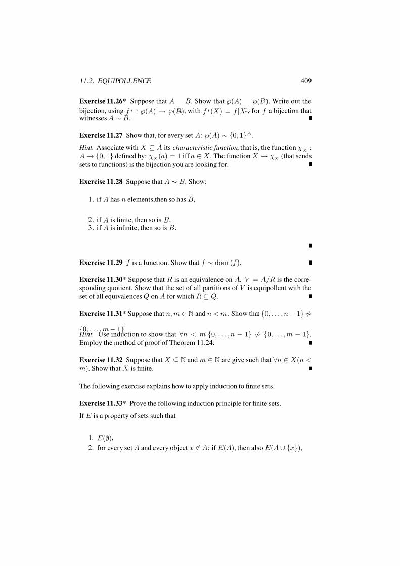
7/16/2019 The Haskell Road to Logic Maths and Programming
http://slidepdf.com/reader/full/the-haskell-road-to-logic-maths-and-programming-5634fa29ef7e9 420/448
11.2. EQUIPOLLENCE 409
Exercise 11.26* Suppose that A
∼B. Show that ℘(A)
∼℘(B). Write out the
bijection, using f ∗ : ℘(A) → ℘(B), with f ∗(X ) = f [X ], for f a bijection thatwitnesses A ∼ B.
Exercise 11.27 Show that, for every set A: ℘(A) ∼ 0, 1A.
Hint. Associate with X ⊆ A its characteristic function, that is, the function χX
:A → 0, 1 defined by: χ
X(a) = 1 iff a ∈ X . The function X → χ
X(that sends
sets to functions) is the bijection you are looking for.
Exercise 11.28 Suppose that A ∼ B. Show:
1. if A has n elements,then so has B,
2. if A is finite, then so is B,3. if A is infinite, then so is B.
Exercise 11.29 f is a function. Show that f ∼ dom (f ).
Exercise 11.30* Suppose that R is an equivalence on A. V = A/R is the corre-
sponding quotient. Show that the set of all partitions of V is equipollent with the
set of all equivalences Q on A for which R ⊆ Q.
Exercise 11.31* Suppose that n, m ∈ N and n < m. Show that 0, . . . , n − 1 ∼
0, . . . , m − 1.
Hint. Use induction to show that ∀n < m 0, . . . , n − 1 ∼ 0, . . . , m − 1.
Employ the method of proof of Theorem 11.24.
Exercise 11.32 Suppose that X ⊆ N and m ∈ N are give such that ∀n ∈ X (n <m). Show that X is finite.
The following exercise explains how to apply induction to finite sets.
Exercise 11.33* Prove the following induction principle for finite sets.
If E is a property of sets such that
1. E (∅),
2. for every set A and every object x ∈ A: if E (A), then also E (A ∪ x),
7/16/2019 The Haskell Road to Logic Maths and Programming
http://slidepdf.com/reader/full/the-haskell-road-to-logic-maths-and-programming-5634fa29ef7e9 421/448
410 CHAPTER 11. FINITE AND INFINITE SETS
then E holds for every finite set.
Hint. Apply induction to the property E of numbers, defined by E (n) ≡ ∀A[Ahas n elements ⇒ E (A)].
Exercise 11.34* Show that a subset of a finite set is finite.
Exercise 11.35* Show that the union of two finite sets is finite.
Exercise 11.36* Suppose that h is a finite injection with dom (h) ⊆ A and
rng (h) ⊆ B. Suppose that A ∼ B. Show that a bijection f : A → B exists
such that f ⊇ h. (And what, if h is infinite?)
Hint. Induction on the number n of elements of h. (The case n = 1 is Exer-cise 11.25.)
Exercise 11.37* Show that a proper subset of a finite set never is equipollent with
that set.
Exercise 11.38 Suppose that A and B are finite sets and f : A → B a bijection.
Show:
1. (B − A) ∼ (A − B),
2. there exists a bijection g : A∪
B→
A∪
B such that f ⊆
g.
Exercise 11.39* Show: a set A is finite iff the following condition is satisfied for
every collection E ⊆ ℘(A): if ∅ ∈ E and ∀B ∈ E ∀a ∈ A (B ∪ a ∈ E ), then
A ∈ E .
11.3 Infinite Sets
One of the great discoveries of Cantor is that for any set A, the set ℘(A) is ‘larger’
(in a sense to made precise below) than A. This shows the existence of ‘Cantor’s
paradise’ of an abundance of sets with higher and higher grades of infinity.

7/16/2019 The Haskell Road to Logic Maths and Programming
http://slidepdf.com/reader/full/the-haskell-road-to-logic-maths-and-programming-5634fa29ef7e9 422/448
11.3. INFINITE SETS 411
At Most Equipollent To
Recall Definition 11.19: sets are equipollent means that there is a bijection be-
tween the two.
Definition 11.40 (At Most Equipollent To) The set A is at most equipollent to Bif an injection exists from A into B.
Notation: A B.
Example 11.41 Z R+.
Theorem 11.42 For every infinite set A: N A.
Proof. Suppose that A is infinite. An injection h : N → A as required can beproduced in the following way.
Note: A = ∅ (since ∅ is finite). Thus, it i s possible to choose an element h(0)∈A.
Now, A = h(0) (for, h(0) is finite). Thus, another element h(1) ∈ A−h(0)exist.
Again, A = h(0), h(1), etc.
Going on, this argument produces different elements h(0), h(1), h(2), . . . in A;
thus, the corresponding function h : N → A is an injection.
Thus, N is the “simplest” infinite set.
Exercise 11.43 Show:
1. A A,
2. A ∼ B =⇒ A B,
3. A B ∧ B C =⇒ A C ,
4. A ⊆ B =⇒ A B,
Exercise 11.44* Show the reverse of Theorem 11.42: if N A, then A is infinite.
Hint. Cf. the proof of Theorem 11.24, p. 408. A slight modification (that uses a
modification of Exercise 11.25) shows that for all n, N 0, . . . , n − 1; this
implies what is required.

7/16/2019 The Haskell Road to Logic Maths and Programming
http://slidepdf.com/reader/full/the-haskell-road-to-logic-maths-and-programming-5634fa29ef7e9 423/448
412 CHAPTER 11. FINITE AND INFINITE SETS
Exercise 11.45 Suppose that h : A
→A is an injection that is not surjective. Say,
b ∈ A − rng (h). Define f : N → A by: f (0) = b, f (n + 1) = h(f (n)). E.g.,f (3) = h(f (2)) = h(h(f (1))) = h(h(h(f (0)))) = h(h(h(b))).
Show that f (n) is different from f (0), . . . , f (n − 1) (n ∈ N). (Induction w.r.t. n.)
Conclusion: f is a injection, and N A.
Exercise 11.46 Show: if N A, then a non-surjective injection h : A → Aexists.
Exercise 11.47 Show: a set is infinite iff it is equipollent with one of its proper
subsets.
Hint. Use Theorem 11.42 and Exercises 11.44, 11.45 and 11.46.
Exercise 11.48 Suppose that A is finite and that f : A → A. Show: f is surjectiveiff f is injective.
Hint. ⇐ : use Exercises 11.44 and 11.45.
Countably Infi nite
The prototype of a countably infinite set is N.
Definition 11.49 (Countable) A set A is countably infinite (or: denumerable) if
N ∼ A.
Exercise 11.50* Show: a subset of a countably infinite set is countably infinite or
finite.
Exercise 11.51 Show:
1. Z (the set of integers) is countably infinite,
2. a union of two countably infinite sets is countably infinite.
Theorem 11.52 N2 = (n, m) | n, m ∈ N is countably infinite.
Proof. Define S ( p) =
(n, m)|
n + m = p
.
The sets S ( p) are pairwise disjoint, and N2 = S (0) ∪ S (1) ∪ S (2) ∪ . . . Moreover,
S ( p) has exactly p+1 elements: (0, p),(1, p−1), . . . ,( p, 0). Verify that the function

7/16/2019 The Haskell Road to Logic Maths and Programming
http://slidepdf.com/reader/full/the-haskell-road-to-logic-maths-and-programming-5634fa29ef7e9 424/448
11.3. INFINITE SETS 413
j : N2
→N that is defined by j(n, m) = 1
2 (n + m)(n + m + 1) + n enumerates
the pairs of the subsequent sets S ( p).
Note that the function j enumeratesN2 as follows:
(0, 0), (0, 1), (1, 0), (0, 2), (1, 1), (2, 0), (0, 3), (1, 2), (2, 1), (3, 0), . . .
Look at all pairs (n, m) as the corresponding points in two-dimensional space.
Visualize j as a walk along these points.
Of course, there are many other “walks” along these points that prove this theorem.
E.g., (visualize!)
(0, 0), (1, 0), (1, 1), (0, 1), (0, 2), (1, 2), (2, 2), (2, 1), (2, 0), (3, 0), (3, 1), . . .
Theorem 11.53 The set of positive rationalsQ+
is countably infinite.
Proof. Identify a positive rational q ∈ Q+ with the pair (n, m) ∈ N2 for which q =nm
and for which n and m are co-prime. Use Theorem 11.52 and Exercise 11.50.
Exercise 11.54 Show that Q is countably infinite.
Exercise 11.55 Show that N∗ is countably infinite.
Exercise 11.56 Show that a union of countably infinitely many countably infinite
sets is countably infinite.
Uncountable
Definition 11.57 (Less Power Than) A set A has power less than B if both A B and A ∼ B.
Notation: A ≺ B.
Thus:
A ≺ B ⇐⇒ A B ∧ A ∼ B.
Example 11.58 0, . . . , n − 1 ≺ N (Theorem 11.24);
N ≺ R (Theorem 11.60).
Warning. That A ≺ B implies but is not equivalent with: there exists a non-
surjective injection from A into B.
7/16/2019 The Haskell Road to Logic Maths and Programming
http://slidepdf.com/reader/full/the-haskell-road-to-logic-maths-and-programming-5634fa29ef7e9 425/448
414 CHAPTER 11. FINITE AND INFINITE SETS
That A
≺B means by definition: A
B and A
∼B. That A
B means that an
injection f : A → B exists. If, moreover, A ∼ B, then no bijection exists betweenA and B; in particular, the injection f cannot be surjective.
Counter-examples to the converse: (Example 11.20) the successor-function n −→n + 1 is a non-surjective injection : N → N, but of course it is false that N ≺ N;
the identity function 1N is a non-surjective injection from N into Q, but we do not
have (Exercise 11.54), that N ≺ Q.
Definition 11.59 (Uncountable) A set A is uncountable in case N ≺ A.
The following is Cantor’s discovery.
Theorem 11.60 R is uncountable.
Proof. (i) That N R is clear (Exercise 11.43.3, N ⊆ R). (ii) It must be shown,
that no bijection h : N → R exists. In fact, there is no surjection from N to R.
That is:
Claim. To every function h : N → R there exists a real r such hat r ∈ ran(h).
Proof. Suppose that h : N → R. Write down the decimal expansion for every
real h(n): h(n) = pn + 0.rn0 rn1 rn2 · · · , where pn ∈ Z, pn h(n) < pn + 1, and
decimals rni ∈ 0, 1, 2, . . . , 9. (E.g., −√ 2 = −2 + 0, 15 · · · )
For every n, choose a digit rn ∈ 0, 1, 2, . . . , 9 such that rn = rnn. The real
r = 0, r0r1r2 · · · then differs from h(n) in its n-th decimal digit (n = 0, 1, 2, . . .).
However, even if pn = 0, this does not imply r
= h(n). For, a real can have two
decimal notations. E.g., 0.5000 · · · = 0.4999 · · · . But, a tail of zeros vs. a tail of
nines is the only case for which this happens. So, this problem can be avoided if
we require rn to be different from 0 and 9.
Recall, that ℘(A) = X | X ⊆ A is the collection of all subsets of A (Defini-
tion 4.22, p. 132). The powerset operation produces in a direct way sets of greater
power.
In particular, not every uncountable set is equipollent with R.
Theorem 11.61 A ≺ ℘(A).
Proof. (i) The injection a→
a
from A into ℘(A) shows that A
℘(A).
(ii) To show that A ∼ ℘(A), we exhibit, as in the previous proof, for every function
h : A → ℘(A), an element D ∈ ℘(A) − rng (h).
7/16/2019 The Haskell Road to Logic Maths and Programming
http://slidepdf.com/reader/full/the-haskell-road-to-logic-maths-and-programming-5634fa29ef7e9 426/448
11.3. INFINITE SETS 415
Such an element can be simply described in this context: we take D =
a
∈A
|a ∈ h(a).
If we would have that D ∈ rng (h), then D would be the value of some d ∈ A.
Now there are two cases: either d ∈ D, or d ∈ D.
If d ∈ D, then, by definition of D, we would have that d ∈ h(d) = D: contra-
diction. And if d ∈ D, then, since D = h(d), we would have that d ∈ h(d), and
hence d ∈ D; again a contradiction.
Conclusion: D ∈ rng (h).
Corollary 11.62 1. N ≺ ℘(N) ≺ ℘(℘(N)) ≺ · · · ,2. for every set A there exists a set B such that A ≺ B.
Exercise 11.63 Show:
1. A ≺ A,
2. A B ⇐⇒ A ≺ B ∨ A ∼ B,
3. A ≺ B ∧ B ∼ C =⇒ A ≺ C .
4. What is wrong with the following “ proof ” for 2 ⇒ ?:
Given is that A B. Suppose that f : A → B is an injection.
(a) f is (by accident) surjective. Then A ∼ B.
(b) f is not surjective. Then A ∼ B, hence A ≺ B.
Exercise 11.64 Show: if A is finite, then A ≺ N.
(The converse of this is true as well)
Exercise 11.65 Show: the real interval (0, 29 ] = r ∈ R | 0 < r 2
9 is uncount-
able.
Exercise 11.66 A is a set. Define h : A → ℘(A) by h(a) = a. Determine
a ∈ A | a ∈ h(a).
Exercise 11.67 Show that N ≺ 0, 1N.
Exercise 11.68* Show that N ≺ NN
. (NN
is the set of all functions : N → N.)
Hint. Produce, for every function ϕ : N → NN, a function f ∈ NN − rng (ϕ).
7/16/2019 The Haskell Road to Logic Maths and Programming
http://slidepdf.com/reader/full/the-haskell-road-to-logic-maths-and-programming-5634fa29ef7e9 427/448
416 CHAPTER 11. FINITE AND INFINITE SETS
Exercise 11.69 Suppose that h : N
→Q is surjective and that we apply the
procedure from the proof of Theorem 11.60 to h to produce a real r. Is r a rationalor not?
*Cantor-Bernstein Theorem
The following result is of fundamental importance in the theory of equipollence.
Theorem 11.70 (Cantor-Bernstein) A B ∧ B A =⇒ A ∼ B.
The proof of this theorem is delegated to the exercises.
Note that we have two examples of uncountable sets: R (Theorem 11.60) and ℘(N)
(Theorem 11.61). It turns out that these sets are of the same magnitude.
Theorem 11.71 R ∼ ℘(N).
Proof. We show that R ℘(Q) ∼ ℘(N) ∼ 0, 1N R. From this, the Cantor-
Bernstein Theorem produces the required conclusion.
1. R ℘(Q). The function r −→ q ∈Q | q < r is an injection from R into
℘(Q).
2. ℘(Q) ∼ ℘(N). Choose a bijection h : Q → N (Exercise 11.54, p. 413). Now
X −→ h[X ] is a bijection between ℘(Q) and ℘(N) (Exercise 11.26, p. 409).
3. ℘(N) ∼ 0, 1N. Cf. Exercise 11.27.
4. 0, 1N R. Associate with h : N → 0, 1 the real (in the interval [0, 19 ]) thathas decimal expansion 0, h(0)h(1)h(2) · · · .
Continuum Problem and Hypothesis.
Since N ≺ R, it is tempting to ask whether sets A exist such that N ≺ A ≺ R.
(If so, such an A exists for which A ⊆ R.) This question is Cantor’s Continuum
Problem. (The continuum is the set R.)
Cantor’s Continuum Hypothesis asserts that such a set does not exist.
The usual set-theoretic axioms cannot answer the question. Godel proved in 1938
that the axioms cannot show that the Continuum Hypothesis is false. Cohen
proved in 1963 that the axioms cannot show that the Continuum Hypothesis is
true. Indeed, as far as the axioms are concerned, the power of R can be unimag-
inably big and there can be arbitrarily many sets A , B , C , . . . ⊆ R such that
N ≺ A ≺ B ≺ C ≺ · · · ≺ R.

7/16/2019 The Haskell Road to Logic Maths and Programming
http://slidepdf.com/reader/full/the-haskell-road-to-logic-maths-and-programming-5634fa29ef7e9 428/448
11.3. INFINITE SETS 417
Example 11.72 We show that [0, 1]
∼[0, 1). Although these intervals differ in
only one element, establishing a bijection between them is far from trivial. (Thereader who doubts this should give it a try before reading on.) Let f : [0, 1] →[0, 1) be an arbitrary injection; say, f (x) = 1
2x. Consider the following function
h : [0, 1] → [0, 1): h sends 1 to f (1) = 12 , 1
2 to f ( 12 ) = 1
4 , 14 to f ( 1
4 ) = 18 etc.; on
other arguments r = 2−n in [0, 1], you let h(r) = r.
Verify that h is bijective. To check injectivity, let r = s ∈ [0, 1]. If neither of r, sis of the form 2−n, then by definition of h we have h(r) = r = s = h(s). If both
are of the form 2−n, say r = 2−i and s = 2−j with i = j, then, by definition
of h, h(r) = 2−i−1 = 2−j−1 = h(s). If one of r, s is of the form 2−n and the
other is not, then one of h(r), h(s) is of the form 2−n and the other is not, so again
h(r) = h(s). This shows that h is injective. For surjectivity, let r ∈ [0, 1). If r is
not of the form 2−n then h(r) = r, so there is an s ∈ [0, 1] with h(s) = r. If r is
of the form 2−n
, say r = 2−i
with i > 0, then h(2−i+1
) = 2−i
= r. Again, thereis an s ∈ [0, 1] with h(s) = r.
Lemma 11.73 If A B ⊆ A , then A ∼ B.
Exercise 11.74* Prove the Lemma.
Hint. Generalize the solution for Example 11.72.
Exercise 11.75* Prove Theorem 11.70.
Hint. Apply Lemma 11.73 to the composition of the two functions that are given.
Exercise 11.76 Show the following variations on the fact that [0, 1] ∼ [0, 1):
1. [0, 1] ∼ [0, 23 ),
2. (x, y) | x2 + y2 1 ∼ (x, y) | x2 + y2 < 1,
3. (x, y) | x2 + y2 1 ∼ (x, y) | |x|, |y| < 12.
Exercise 11.77* Suppose that A ⊆ R is finite or countably infinite. Show that
R
−A is uncountable. Can you show that (R
−A)
∼R?
Exercise 11.78 Show that (R−Q) ∼ R.

7/16/2019 The Haskell Road to Logic Maths and Programming
http://slidepdf.com/reader/full/the-haskell-road-to-logic-maths-and-programming-5634fa29ef7e9 429/448
418 CHAPTER 11. FINITE AND INFINITE SETS
11.4 Cantor’s World Implemented
The following program illustrates that N2 is denumerable:
natpairs = [(x,z-x) | z <- [0..], x <- [0..z]]
This gives:
FAIS> natpairs
[(0,0),(0,1),(1,0),(0,2),(1,1),(2,0),(0,3),(1,2),(2,1),
(3,0),(0,4),(1,3),(2,2),(3,1),(4,0),(0,5),(1,4),(2,3),
(3,2),(4,1),(5,0)Interrupted!
Exercise 11.79 Implement the function pair :: (Int,Int) -> Int that is theinverse of natpairs. It should hold for all natural numbers n that
pair (natpairs !! n) = n.
Exercise 11.80 Implement a function natstar :: [[Int]] to enumerate N∗
(cf. Exercise 11.55).
The following code illustrates that Q is denumerable:
rationals = [ (n,m) | (n,m) <- natpairs, m /= 0, gcd n m == 1 ]
This gives:
FAIS> rationals
[(0,1),(1,1),(1,2),(2,1),(1,3),(3,1),(1,4),(2,3),(3,2),(4,1),(1,5),
(5,1),(1,6),(2,5),(3,4),(4,3),(5,2),(6,1),(1,7),(3,5),(5,3),(7,1),
(1,8),(2,7),(4,5),(5,4),(7,2),(8,1),(1,9),(3,7),(7,3),(9,1),(1,10),
(2,9),(3,8),(4,7),(5,6),(6,5),(7,4),(8,3),(9,2),(10,1),(1,11),(5,7),(7,5),(11,1),(1,12),(2,11),(3,10),(4,9),(5,8),(6,7),(7,6),(8,5),(9,4),
(10,3),(11,2),(12,1),(1,13),(3,11),(5,9),(9,5),(11,3),(13,1),(1,14),
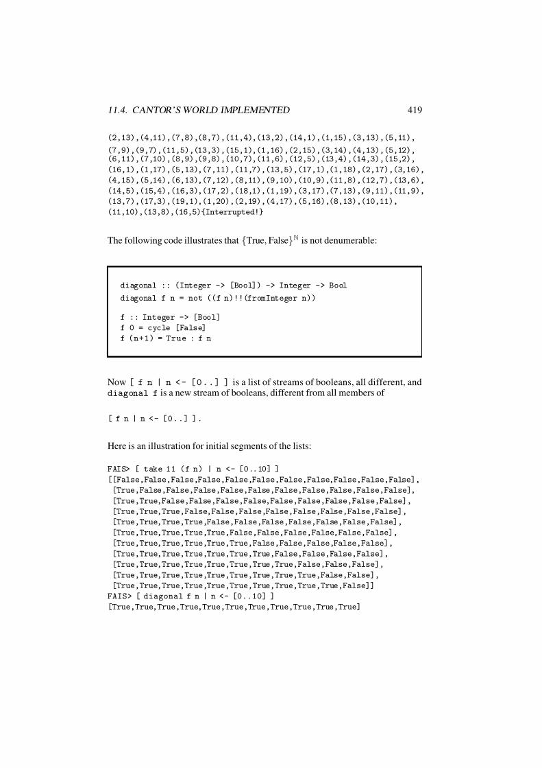
7/16/2019 The Haskell Road to Logic Maths and Programming
http://slidepdf.com/reader/full/the-haskell-road-to-logic-maths-and-programming-5634fa29ef7e9 430/448
11.4. CANTOR’S WORLD IMPLEMENTED 419
(2,13),(4,11),(7,8),(8,7),(11,4),(13,2),(14,1),(1,15),(3,13),(5,11),
(7,9),(9,7),(11,5),(13,3),(15,1),(1,16),(2,15),(3,14),(4,13),(5,12),(6,11),(7,10),(8,9),(9,8),(10,7),(11,6),(12,5),(13,4),(14,3),(15,2),
(16,1),(1,17),(5,13),(7,11),(11,7),(13,5),(17,1),(1,18),(2,17),(3,16),
(4,15),(5,14),(6,13),(7,12),(8,11),(9,10),(10,9),(11,8),(12,7),(13,6),
(14,5),(15,4),(16,3),(17,2),(18,1),(1,19),(3,17),(7,13),(9,11),(11,9),
(13,7),(17,3),(19,1),(1,20),(2,19),(4,17),(5,16),(8,13),(10,11),
(11,10),(13,8),(16,5)Interrupted!
The following code illustrates that True, FalseN is not denumerable:
diagonal :: (Integer -> [Bool]) -> Integer -> Bool
diagonal f n = not ((f n)!!(fromInteger n))
f :: Integer -> [Bool]
f 0 = cycle [False]
f (n+1) = True : f n
Now [ f n | n < - [ 0 . . ] ] is a list of streams of booleans, all different, anddiagonal f is a new stream of booleans, different from all members of
[ f n | n <- [0..] ].
Here is an illustration for initial segments of the lists:
FAIS> [ take 11 (f n) | n <- [0..10] ]
[[False,False,False,False,False,False,False,False,False,False,False],
[True,False,False,False,False,False,False,False,False,False,False],
[True,True,False,False,False,False,False,False,False,False,False],
[True,True,True,False,False,False,False,False,False,False,False],
[True,True,True,True,False,False,False,False,False,False,False],
[True,True,True,True,True,False,False,False,False,False,False],
[True,True,True,True,True,True,False,False,False,False,False],
[True,True,True,True,True,True,True,False,False,False,False],
[True,True,True,True,True,True,True,True,False,False,False],
[True,True,True,True,True,True,True,True,True,False,False],
[True,True,True,True,True,True,True,True,True,True,False]]
FAIS> [ diagonal f n | n <- [0..10] ]
[True,True,True,True,True,True,True,True,True,True,True]

7/16/2019 The Haskell Road to Logic Maths and Programming
http://slidepdf.com/reader/full/the-haskell-road-to-logic-maths-and-programming-5634fa29ef7e9 431/448
420 CHAPTER 11. FINITE AND INFINITE SETS
11.5 *Cardinal Numbers
By Theorem 11.21, equipollence is an equivalence on the collection of all sets.
Definition 11.81 (Cardinal Number) A cardinal number is an equivalence class
w.r.t. equipollence.
|A| denotes the cardinal number of the set A modulo ∼.
The following is immediate (cf. Lemma 5.80, p. 193):
Lemma 11.82 |A| = |B| ⇐⇒ A ∼ B.
Usually, the cardinal number |0, . . . , n − 1| of the n-element sets is identified
with the natural number n.
Aleph-zero. ℵ0 = |N|.1
The concept of a cardinal number can be considered as a generalisation of that of
a natural number.
It is possible to generalize the definitions of addition, multiplication and exponen-
tiation to cardinal numbers, and to prove natural laws that generalize those for the
natural numbers.
The operations are defined as follows. |A|+ |B| = |A∪B| (provided that A∩B =∅: only if A and B are disjoint sets of n resp. m elements does it follow that their
union has n + m elements), |A| × |B| = |A × B| and |A||B| = |AB|.Thus, by Theorem 11.71, we have that |R| = 2ℵ0 .
The cardinal ℵ0 is the starting point of an infinite series of cardinal numbers called
alephs: ℵ0 < ℵ1 < ℵ2 < · · · < ℵω < · · · ; (ℵω is the smallest cardinal bigger
than every ℵn).
Using cardinals sometimes makes for amazingly compact proofs. An example is
the following theorem.
Theorem 11.83 R × R ∼ R , i.e.: there are as many points in the plane as on a
line.
1ℵ (aleph) is the fi rst letter of the Hebrew alphabet.

7/16/2019 The Haskell Road to Logic Maths and Programming
http://slidepdf.com/reader/full/the-haskell-road-to-logic-maths-and-programming-5634fa29ef7e9 432/448
11.5. CARDINAL NUMBERS 421
Proof.
|R× R| = |R| × |R|= 2ℵ0 × 2ℵ0
= 2ℵ0+ℵ0
= 2ℵ0
= |R|.The third equality uses the rule n p× nq = n p+q , the fourth that ℵ0 + ℵ0 = ℵ0, cf.
Exercise 11.51, p. 412.
*Further Exercises
Exercise 11.84 Suppose that A1 ∼ A2 and B1 ∼ B2. Show:
1. if A1 ∩ B1 = A2 ∩ B2 = ∅, then A1 ∪ B1 ∼ A2 ∪ B2,
2. A1 × B1 ∼ A2 × B2,
3.* AB11 ∼ AB2
2 (Hint: it does not do to say |A1B1 | = |A1||B1| = |A2||B2| =
|A2B2 |, for we don’t have a rule of exponentiation for cardinal numbers as
yet. Instead, show how to establish a bijection between AB11 and AB2
2 .)
Exercise 11.85 Suppose that A1 A2 and B1 B2. Show:
1. if A2 ∩ B2 = ∅, then A1 ∪ B1 A2 ∪ B2,
2. A1 × B1 A2 × B2,
3. ℘(A1) ℘(A2),
4.* if A2 = ∅, then AB11 AB2
2 (Hint: Use the fact that, since A2 = ∅, you
can pick a ∈ A2 for the definition of the injection that you need.)
Exercise 11.86 Give counter-examples to the following implications:
1. A1 ≺ A2 ⇒ A1 ∪ B ≺ A2 ∪ B (A1 ∩ B = A2 ∩ B = ∅),
7/16/2019 The Haskell Road to Logic Maths and Programming
http://slidepdf.com/reader/full/the-haskell-road-to-logic-maths-and-programming-5634fa29ef7e9 433/448
422 CHAPTER 11. FINITE AND INFINITE SETS
2. A1
≺A2
⇒A1
×B
≺A2
×B,
3. A1 ≺ A2 ⇒ AB1 ≺ AB
2 ,
4. A1 ≺ A2 ⇒ BA1 ≺ BA2 .
Exercise 11.87 Show:
1. if B ∩ C = ∅, then AB∪C ∼ AB × AC ,
2. (A × B)C ∼ AC × BC
3.* (AB)C
∼AB×C . (Hint: use the currying operation.)
Exercise 11.88 Show (n 1):
1. 0, 1N ∼ 0, . . . , nN ∼ NN ∼ RN ∼ R,
2. 0, 1R ∼ 0, . . . , nR ∼ NR ∼ RR ∼ (℘(R))R ∼ (RR)R.
Exercise 11.89 Show, for all n ∈ N+: Nn ∼ N (n.b.: NN ∼ N) and Rn ∼ R (n.b.:
RN
∼R).
Exercise 11.90 Show: (x, y) ∈ R2 | x2 + y2 1 ∧ y > 0 ∼ (x, y) ∈ R2 |1 < y 2.
Exercise 11.91 Show: if A is infinite and B finite, then (A − B) ∪ (B − A) ∼ A.
7/16/2019 The Haskell Road to Logic Maths and Programming
http://slidepdf.com/reader/full/the-haskell-road-to-logic-maths-and-programming-5634fa29ef7e9 434/448
The Greek Alphabet
Mathematicians are in constant need of symbols, and most of them are very fond
of Greek letters. Since this book might be your first encounter with this new set of
symbols, we list the Greek alphabet below.
name lower case upper case
alpha αbeta β gamma γ Γdelta δ ∆epsilon εzeta ζ eta ηtheta θ Θiota ι
kappa κlambda λ Λmu µnu ν xi ξ Ξpi π Πrho ρsigma σ Σtau τ upsilon υ Υphi ϕ Φchi χpsi ψ Ψ
omega ω Ω
423

7/16/2019 The Haskell Road to Logic Maths and Programming
http://slidepdf.com/reader/full/the-haskell-road-to-logic-maths-and-programming-5634fa29ef7e9 435/448
424
7/16/2019 The Haskell Road to Logic Maths and Programming
http://slidepdf.com/reader/full/the-haskell-road-to-logic-maths-and-programming-5634fa29ef7e9 436/448
Bibliography
[AHV95] S Abiteboul, R. Hull, and V. Vianu. Foundations of Databases. Ad-
dison Wesley, 1995.
[Bab61] C. Babbage. On the Principles and Development of the Calculator .
Dover, 1961. Edited and with an introduction by P. Morrison and E.
Morrison.
[Bab94] C. Babbage. Passages from the Life of a Philosopher . Rutgers Uni-
versity Press and IEEE-Press, New Brunswick, New Jersey and Pis-
cataway, New Jersey, 1994. Edited with a new introduction by Martin
Campbell-Kelly. Originally published 1864.
[Bal91] V. K. Balakrishnan. Introductory Discrete Mathematics. Dover, 1991.
[Bar84] H. Barendregt. The Lambda Calculus: Its Syntax and Semantics (2nd
ed.). North-Holland, Amsterdam, 1984.
[Bir98] R. Bird. Introduction to Functional Programming Using Haskell.
Prentice Hall, 1998.
[BM96] J. Barwise and L. Moss. Vicious Circles: On the Mathematics of
Non-wellfounded Phenomena. CSLI Publications, 1996.
[Bry93] V. Bryant. Yet anotherintroduction to analysis. CambridgeUniversity
Press, 1993.
[Bur98] Stanley N. Burris. Logic for Mathematics and Computer Science.
Prentice Hall, 1998.
[CG96] J.H. Conway and R.K. Guy. The Book of Numbers. Springer, 1996.
[CR78] R. Courant and H. Robbins. What is Mathematics? An Elementary
Approach to Ideas and Methods. Oxford University Press, Oxford,
1978.
425

7/16/2019 The Haskell Road to Logic Maths and Programming
http://slidepdf.com/reader/full/the-haskell-road-to-logic-maths-and-programming-5634fa29ef7e9 437/448
426 BIBLIOGRAPHY
[CrbIS96] R. Courant and H. Robbins (revised by I. Stewart). What is Math-
ematics? An Elementary Approach to Ideas and Methods (Second Edition). Oxford University Press, Oxford, 1996.
[Doe96] H.C. Doets. Wijzer in Wiskunde. CWI, Amsterdam, 1996. Lecture
notes in Dutch.
[DP02] B.A. Davey and H.A. Priestley. Introduction to Lattices and Order
(Second Edition). Cambridge University Press, Cambridge, 2002.
First edition: 1990.
[DvDdS78] K. Doets, D. van Dalen, and H. de Swart. Sets: Naive, Axiomatic,
and Applied . Pergamon Press, Oxford, 1978.
[Ecc97] P. J. Eccles. An Introduction to Mathematical Reasoning. Cambridge
University Press, 1997.
[EFT94] H.-D. Ebbinghaus, J. Flum, and W. Thomas. Mathematical Logic.
Springer-Verlag, Berlin, 1994. Second Edition.
[Euc56] Euclid. The Thirteen Books of the Elements, with Introduction and
Commentary by Sir Thomas L. Heath. Dover, 1956.
[Fok00] W. Fokkink. Introduction to Process Algebra. Springer, 2000.
[GKP89] R.L. Graham, D.E. Knuth, and O. Patashnik. Concrete Mathematics.
Addison Wesley, Reading, Mass, 1989.
[Har87] D. Harel. Algorithmics: The Spirit of Computing. Addison-Wesley,
1987.
[HFP96] P. Hudak, J. Fasel, and J. Peterson. A gentle introduction to Haskell.
Technical report, Yale University, 1996. Available from the Haskell
homepage: http://www.haskell.org.
[Hin97] J. Roger Hindley. Basic Simple Type Theory. Cambridge University
Press, 1997.
[HO00] C. Hall and J. O’Donnell. Discrete Mathematics Using A Computer .
Springer, 2000.
[HR00] M. Huth and M. Ryan. Logic in Computer Science: Modelling and
Reasoning about Systems. Cambridge University Press, 2000.
[HT] The Haskell Team. The Haskell homepage. http://www.haskell.
org.

7/16/2019 The Haskell Road to Logic Maths and Programming
http://slidepdf.com/reader/full/the-haskell-road-to-logic-maths-and-programming-5634fa29ef7e9 438/448
BIBLIOGRAPHY 427
[Hud00] P. Hudak. The Haskell School of Expression: Learning Functional
Programming Through Multimedia. Cambridge University Press,2000.
[Jon03] S. Peyton Jones, editor. Haskell 98 Language and Libraries; The
Revised Report . Cambridge University Press, 2003.
[JR+] Mark P. Jones, Alastair Reid, et al. The Hugs98 user manual. http:
//www.haskell.org/hugs/.
[Kar97] J. Karczmarczuk. Generating power of lazy semantics. Theoretical
Computer Science, 187, 1997.
[Knu92] D.E. Knuth. Literate Programming. CSLI Lecture Notes, no. 27.
CSLI, Stanford, 1992.
[Lar34] D. Lardner. Babbage’s calculating engine. Edinburgh Review, 1834.
[McI99] M.D. McIlroy. Power series, power serious. Journal of Functional
Programming, 9:323–335, 1999.
[McI00] M.D. McIlroy. The music of streams. Elsevier Preprints, 2000.
[Mil99] R. Milner. Communicating and Mobile Systems: the π Calculus.
Cambridge University Press, 1999.
[Ore88] O. Ore. Number Theory and its History. Dover, 1988.
[Pol57] G. Polya. How to Solve It. A New Aspect of Mathematical Method .
Princeton University Press, Princeton, 1957.
[RL99] F. Rabhi and G. Lapalme. Algorithms: a Functional Programming
Approach. Addison-Wesley, 1999.
[Rus67] B. Russell. Letter to Frege. In J. van Heijenoord, editor, From Frege
to G ¨ odel, pages 124–125. Harvard University Press, 1967.
[Rut00] J.J.M.M. Rutten. Behavioural differential equations: a coinductive
calculus of streams, automata, and power series. Report SEN-R0023,
CWI, 2000. Available at URL: www.cwi.nl. To appear in Theoretical
Computer Science.
[SKS01] A. Silberschatz, H.F. Korth, and S. Sudarshan. Database System Con-
cepts (4th edition). McGraw-Hill, 2001.
[Tho99] S. Thompson. Haskell: the craft of functional programming (second
edition). Addison Wesley, 1999.

7/16/2019 The Haskell Road to Logic Maths and Programming
http://slidepdf.com/reader/full/the-haskell-road-to-logic-maths-and-programming-5634fa29ef7e9 439/448
428 BIBLIOGRAPHY
[Vel94] D.J. Velleman. How to Prove It. A Structured Approach. Cambridge
University Press, Cambridge, 1994.
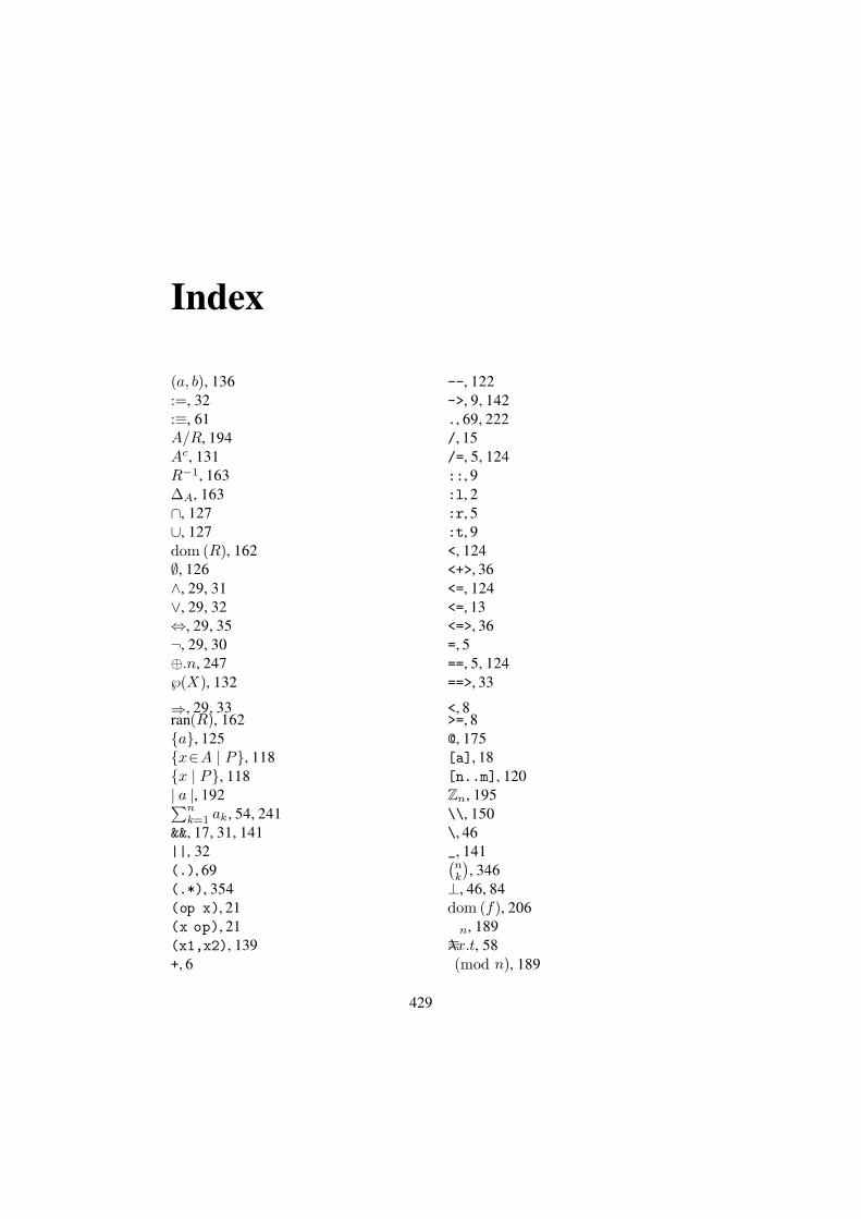
7/16/2019 The Haskell Road to Logic Maths and Programming
http://slidepdf.com/reader/full/the-haskell-road-to-logic-maths-and-programming-5634fa29ef7e9 440/448
Index
(a, b), 136
:=, 32
:≡, 61
A/R, 194
Ac, 131
R−1, 163
∆A, 163
∩, 127
∪, 127
dom (R), 162
∅, 126
∧, 29, 31
∨, 29, 32
⇔, 29, 35
¬, 29, 30
⊕.n, 247
℘(X ), 132
⇒, 29, 33ran(R), 162
a, 125
x∈A | P , 118
x | P , 118
| a |, 192nk=1 ak, 54, 241
&&, 17, 31, 141
||, 32
(.), 69
(.*), 354
(op x), 21
(x op), 21
(x1,x2), 139
+, 6
--, 122
->, 9, 142
., 69, 222
/, 15
/=, 5, 124
::, 9
:l, 2
:r, 5
:t, 9
<, 124
<+>, 36
<=, 124
<=, 13
<=>, 36
=, 5
==, 5, 124
==>, 33
<, 8>=, 8
@, 175
[a], 18
[n..m], 120
Zn, 195
\\, 150
\, 46
_, 141nk
, 346
⊥, 46, 84
dom (f ), 206
≡n, 189
λx.t, 58
(mod n), 189
429
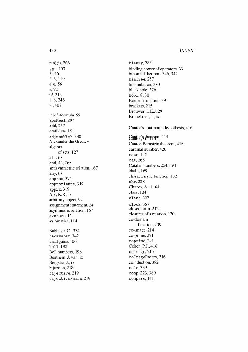
7/16/2019 The Haskell Road to Logic Maths and Programming
http://slidepdf.com/reader/full/the-haskell-road-to-logic-maths-and-programming-5634fa29ef7e9 441/448
430 INDEX
ran(f ), 206nk, 197
, 46
^, 6, 119
d|n, 56
e, 221
n!, 213
|, 6, 246
∼, 407
‘abc’-formula, 59
absReal, 207
add, 267
addElem, 151
adjustWith, 340Alexander the Great, v
algebra
of sets, 127
all, 68
and, 42, 268
antisymmetric relation, 167
any, 68
approx, 375
approximate, 319
apprx, 319
Apt, K.R., ix
arbitrary object, 92
assignment statement, 24
asymmetric relation, 167
average, 15
axiomatics, 114
Babbage, C., 334
backsubst, 342
ballgame, 406
bell, 198
Bell numbers, 198
Benthem, J. van, ix
Bergstra, J., ix
bijection, 218
bijective, 219
bijectivePairs, 219
binary, 288
binding power of operators, 33binomial theorem, 346, 347
BinTree, 257
bisimulation, 380
black hole, 276
Bool, 8, 30
Boolean function, 39
brackets, 215
Brouwer, L.E.J, 29
Brunekreef, J., ix
Cantor’s continuum hypothesis, 416
Cantor’s theorem, 414Cantor, G., 114
Cantor-Bernstein theorem, 416
cardinal number, 420
case, 142
cat, 265
Catalan numbers, 254, 394
chain, 169
characteristic function, 182
chr, 228
Church, A., 1, 64
class, 124
class, 227
clock, 367closed form, 212
closures of a relation, 170
co-domain
function, 209
co-image, 214
co-prime, 291
coprime, 291
Cohen, P.J., 416
coImage, 215
coImagePairs, 216
coinduction, 382
cols, 339
comp, 223, 389
compare, 141

7/16/2019 The Haskell Road to Logic Maths and Programming
http://slidepdf.com/reader/full/the-haskell-road-to-logic-maths-and-programming-5634fa29ef7e9 442/448
INDEX 431
comparison property, 169
completeness, 168complex numbers, 320
complR, 178
composition
function –, 69, 222
confluence, 404
congruence, 236
conjunction, 31
constructor, 12
constructor identifier, 12
continue, 335
continuity, 66, 315
continuum problem, 416contradiction, 48
contraposition, 35
converse, 35
conversion, 15
convolution, 354
Coquand, T., ix
corecursion, 362
corecursive definition, 362
countable, 412
curry, 183
Curry, H.B., 1, 183
curry3, 210
CWI, ix
data, 139, 257
data, 30, 145
database query, 145
decExpand, 307
decForm, 308
decodeFloat, 311
deduction rule, 78
default, 362
delete, 149
deleteSet, 156
delta, 355
denumerable, 412
deriv, 358
deriving, 140
destructive assignment, 24diagonal, 419
difLists, 334
difs, 332
disjunction, 32
display, 158
div, 20
divergence, 122
divides, 5, 183
domain, 162
Double, 17, 311
e2o, 397echelon, 341
echelon matrix form, 338
elem, 123
elem, 151
elem’, 150
elemIndex, 308
eliminate, 341
else, 230
emptySet, 156
encodeFloat, 312
Enum, 227
enum_2, 107
EQ, 141Eq , 124, 246
eq , 184
eq1, 298
equalSize, 190
equation guarding, 6
equational reasoning, 24
equipollent, 406
equiv2listpart,199
equiv2part, 199
equivalence, 35
equivalence, 188
equivalence’, 188
Eratosthenes
sieve of —, 105
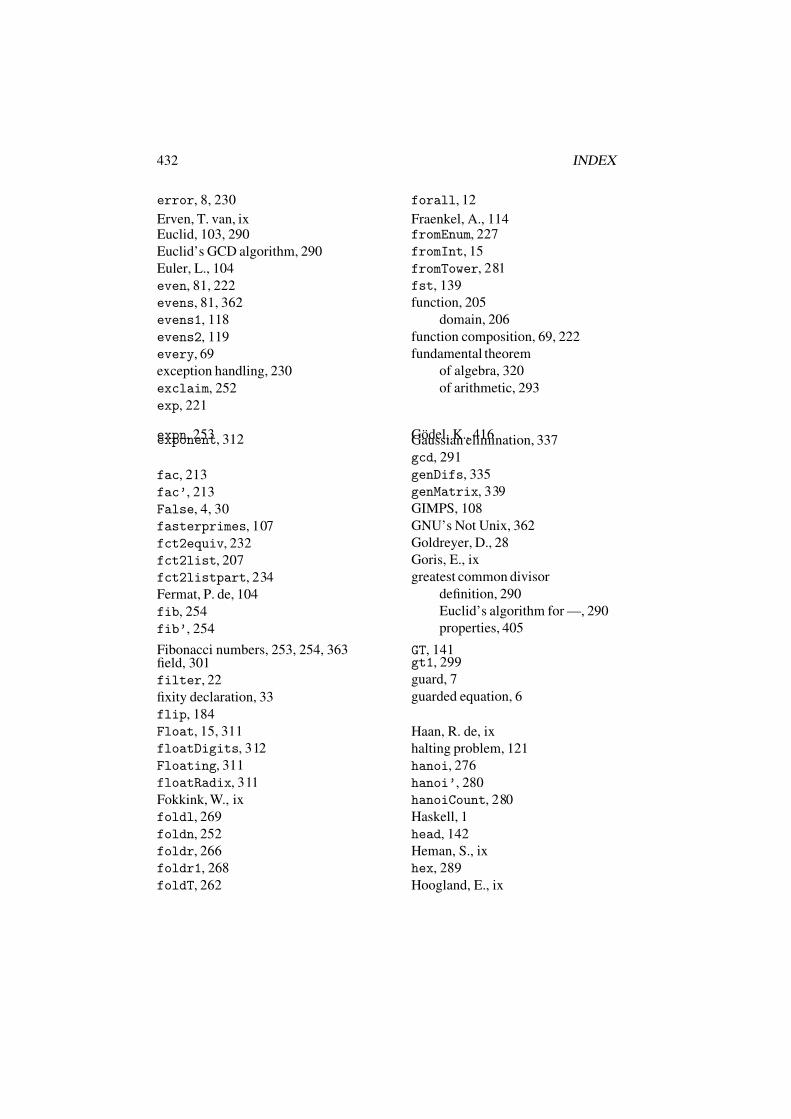
7/16/2019 The Haskell Road to Logic Maths and Programming
http://slidepdf.com/reader/full/the-haskell-road-to-logic-maths-and-programming-5634fa29ef7e9 443/448
432 INDEX
error, 8, 230
Erven, T. van, ixEuclid, 103, 290
Euclid’s GCD algorithm, 290
Euler, L., 104
even, 81, 222
evens, 81, 362
evens1, 118
evens2, 119
every, 69
exception handling, 230
exclaim, 252
exp, 221
expn, 253exponent, 312
fac, 213
fac’, 213
False, 4, 30
fasterprimes, 107
fct2equiv, 232
fct2list, 207
fct2listpart, 234
Fermat, P. de, 104
fib, 254
fib’, 254
Fibonacci numbers, 253, 254, 363field, 301
filter, 22
fixity declaration, 33
flip, 184
Float, 15, 311
floatDigits, 312
Floating, 311
floatRadix, 311
Fokkink, W., ix
foldl, 269
foldn, 252
foldr, 266
foldr1, 268
foldT, 262
forall, 12
Fraenkel, A., 114fromEnum, 227
fromInt, 15
fromTower, 281
fst, 139
function, 205
domain, 206
function composition, 69, 222
fundamental theorem
of algebra, 320
of arithmetic, 293
Godel, K., 416Gaussian elimination, 337
gcd, 291
genDifs, 335
genMatrix, 339
GIMPS, 108
GNU’s Not Unix, 362
Goldreyer, D., 28
Goris, E., ix
greatest common divisor
definition, 290
Euclid’s algorithm for —, 290
properties, 405
GT, 141gt1, 299
guard, 7
guarded equation, 6
Haan, R. de, ix
halting problem, 121
hanoi, 276
hanoi’, 280
hanoiCount, 280
Haskell, 1
head, 142
Heman, S., ix
hex, 289
Hoogland, E., ix
7/16/2019 The Haskell Road to Logic Maths and Programming
http://slidepdf.com/reader/full/the-haskell-road-to-logic-maths-and-programming-5634fa29ef7e9 444/448
INDEX 433
id, 207
idR, 175Iemhoff, R., ix
if then else, 230
iff, 30
ILLC, ix
image, 214
image, 215
imagePairs, 216
implication, 33
import, 72
in, 15
induction, 239, 240, 400
strong, 401infinity
of primes, 103
infix, 4
infix, 33
infix notation, 21
infixl, 156
infixr, 156
init, 143
injection, 218
injective, 219
injectivePairs, 219
injs, 221
inorder tree traversal, 262inR, 178
insertSet, 156
inSet, 155
instance
of a type class, 124
instance, 140
Int, 11
int, 388
Integer, 9, 11
integers, 294
Integral, 11
integral rational functions, 331
intersect, 150
intransitive relation, 168
intToDigit, 288, 289
intuitionism, 29inverse, 184
invR, 178
irrational numbers, 311
irrationality
of √
2, 309
irreflexive relation, 166
irreflR, 179
isAlpha, 232
isEmpty, 156
iterate, 313, 336, 363
Jongh, D. de, ix
Just, 231
Kaldewaij, A., ix
labeled transition system, 365
lambda abstraction, 46, 58, 145, 211
lambda term, 58
last, 143
law
associativity, 46, 247, 249
commutativity, 46, 247, 249
contraposition, 45
DeMorgan, 46, 132
distribution, 46
distributivity, 249
dominance, 48
double negation, 45
excluded middle, 48
idempotence, 45
identity, 48
lazy list, 23, 105
lazy pattern, 373
LD, 4
ldp, 23
ldpf, 23
leaf tree, 263
LeafTree, 263
left triangular matrix form, 338
7/16/2019 The Haskell Road to Logic Maths and Programming
http://slidepdf.com/reader/full/the-haskell-road-to-logic-maths-and-programming-5634fa29ef7e9 445/448
434 INDEX
len, 265
length, 15leq , 250
leq1, 299
lessEq , 184
let, 15
lexicographical order, 141
limit, 315
linear relation, 169
list, 16, 139
list comprehension, 42, 54, 118
list2fct, 207
list2set, 156
listpart2equiv, 199listPartition,199
listRange, 208
lists, 139
listValues, 208
ln, 267
ln’, 272
load Haskell file, 2
logBase, 281
LT, 141
Lucas numbers, 394
Main>, 5
mantissa, 311 map, 21, 151, 272
mapLT, 264
mapR, 264
mapT, 261
Matrix, 338
matrix, 338
maxBound, 208
Maybe, 231
maybe, 231
mechanic’s rule, 313
mechanics, 313
mechanicsRule,313
Menaechmus, v
Mersenne, M., 104
min, 13
minBound, 208 mkStdGen, 366
mlt, 267
mnmInt, 13
mod, modulo, 190
module, 2
modulo, 190
Modus Ponens, 80
mult, 252
mult1, 298
mySqrt, 319
n-tuples, 139
Napier’s number, 221, 395natpairs, 418
natstar, 418
Natural, 246
natural logarithm, 221
natural number, 246
naturals, 118, 362
necessary condition, 35
negate, 222
negation, 30
Newman’s Lemma, 404
Newman, B., 28
Newton’s method, 313
Newton, I., 346
newtype, 153
next, 335
nextD, 335
nondeterminism, 365
not, 30
notElem, 151
Nothing, 231
Nuallain, B. O, ix
nub, 144
null, 143
Num, 124
o2e, 396
odd, 222

7/16/2019 The Haskell Road to Logic Maths and Programming
http://slidepdf.com/reader/full/the-haskell-road-to-logic-maths-and-programming-5634fa29ef7e9 446/448
INDEX 435
odds, 362
odds1, 119oddsFrom3, 107
of, 142
one-to-one, 218
ones, 125
ones, 362
onto, 218
Oostrom, V. van, ix
open problems, 109, 111
operation, 236
operator precedence, 42
or, 268
Ord, 124Ord, 141
ord, 228
order
partial —, 168
strict partial —, 168
total —, 169
Ordering, 141
otherwise, 7
overloading, 125
p2fct, 343
pair, 418
pairs, 136paradox
halting —, 121
Russell —, 120
part2error, 231
partial functions, 229
partial order, 168
Pascal’s triangle, 348
Pascal, B., 348
pattern matching, 13, 143, 250
perms, 221
Platonism, 28
plus, 247
plus, 252
plus1, 298
po-set reflection, 195
polynomial, 320polynomials, 331
polynomials and coefficient lists, 344
Ponse, A., ix
postorder tree traversal, 262
power series, 387
powerList, 151
powerSet, 156
pre, 253
pre-order, 168
pred, 227
prefix, 4
prefix, 17prefix notation, 21
Prelude>, 2
Prelude, 26
preorder tree traversal, 262
primCompAux, 142
prime, 23
prime factorization algorithm, 19
prime’’, 165
prime0, 8
primes
definition, 60
Mersenne —, 105
primes, 106primes’, 364
primes0, 22
primes1, 23
principle
comprehension —, 114
minimality —, 402
Process, 366
product
of sets, 136
product, 213
propositional function, 39
ptd, 369
quasi-order, 168

7/16/2019 The Haskell Road to Logic Maths and Programming
http://slidepdf.com/reader/full/the-haskell-road-to-logic-maths-and-programming-5634fa29ef7e9 447/448
436 INDEX
quotient, 194
quotient, 251quotRem, 286
raccess, 194
random numbers, 366
random streams, 366
Random.hs, 361
randomInts, 366
randomRs, 366
ranPairs, 208
Rational, 341
rationals, 299
countability of —, 413rationals, 418
rclosR, 182
reals, 310
uncountability of —, 414
recip, 313
recurrence, 212
recursion, 246
recursive definition, 7, 246
reduce1, 298
reflect, 264
reflexive closure, 171
reflexive relation, 166
reflexive transitive closure, 171reflR, 178
relation
antisymmetric —, 167
asymmetric —, 167
between, 162
domain, 162
from—to, 162
intransitive —, 168
irreflexive —, 166
linear —, 169
range, 162
reflexive —, 166
symmetric —, 166
transitive —, 167
relatively prime, 291
reload Haskell file, 5rem, 5
remainder, 251
removeFst, 14
reserved keywords, 12
restrict, 214
restrictPairs,214
restrictR, 182
rev, 269
rev’, 270
rev1, 272
Rodenburg, P., ix
rose tree, 264rows, 339
royal road to mathematics, v
Russell, B., 57, 120
Rutten, J., ix
sclosR, 182
sections, 21
Set a, 153
Show, 246
showDigits, 289
showSet, 155
sieve, 106, 364
sieve of Eratosthenes, 105sieve’, 364
significand, 312
sin, 221
singleton, 125
small_squares1,119
small_squares2,120
Smullyan’s ball game, 405
Smullyan, R., 405
snd, 139
solveQdr, 59
solveSeq , 342
solving quadratic equations, 59
some, 69
soundness, 168
7/16/2019 The Haskell Road to Logic Maths and Programming
http://slidepdf.com/reader/full/the-haskell-road-to-logic-maths-and-programming-5634fa29ef7e9 448/448
INDEX 437
space leak, 276
split, 263splitAt, 308
splitList, 144
sqrt, 59, 221
sqrtM, 313
srtInts, 14
start, 366
stirling, 198
Stirling set numbers, 198
stream, 362
stream bisimulation, 383
strict partial order, 168
String, 16String, 16
stringCompare,232
sub domain, 53
substitution principle, 48
subtr, 251
subtr, 253
subtr1, 298
succ, 227
successor, 246
sufficient condition, 35
sum, 241
sum, 15, 54, 241
sumCubes, 245sumCubes’, 245
E 242
symmetric relation, 166
symR, 179
tail, 142
take, 107
takeWhile, 313
tan, 221
tclosR, 182
Terlouw, J., ix
theFibs, 363
then, 230
theNats, 363
theNats1, 363
theOdds, 363theOnes, 363
toBase, 289
toEnum, 227
total order, 169
totalR, 178
toTower, 281
tower of Hanoi, 273
transClosure’,187
transition system, 365
transitive closure, 171
transitive relation, 167
transR, 179
treeleaf –, 263
264