the heckscher-ohlin model · 3 introduction the heckscher-ohlin (ho) model, a model that assumes...

R.López-Monti -1

The Heckscher-Ohlin Model

SURVEY OF INTERNATIONAL

ECONOMICS

Rafael López-MontiDepartment of Economics

George Washington University

[email protected]

Summer 2015(Econ 6280.20)

Required Reading:

Feenstra, R. and Taylor, A., International Economics (3e). Worth Publishers, CHAPTER 4

OR Feenstra, R. and Taylor, A., Essential of International Economics (3e). Worth Publishers, CHAPTER 4

* Material for teaching only. Please do not cite or circulate. Some typos might remain

2

TRADE AND RESOURCES

Heckscher-Ohlin Model

Testing the Heckscher-Ohlin Model

Effects of Trade on Factor Prices

3

Introduction

the Heckscher-Ohlin (HO) model, a model that assumes that trade

occurs because countries have different resources.

Canada has a large amount of land and therefore exports agricultural

and forestry products, as well as petroleum.

The United States, Western Europe, and Japan have relatively many

high-skilled workers and much capital and these countries export

sophisticated services and manufactured goods.

China and other Asian countries have a large number of workers and

moderate but growing amounts of capital and they export less

sophisticated manufactured goods.

4

Heckscher-Ohlin Model: Assumptions

Assumption 1

Two factors of production, labor (L) and capital (K), can move freely

between the industries.

Assumption 2

Two goods: shoe (S) and computers (C). Shoe production is relatively

labor-intensive; that is, it requires more labor per unit of capital to

produce shoes than computers.

𝑳𝑺 𝑲𝑺 > 𝑳𝑪 𝑲𝑪

5

Heckscher-Ohlin Model: Assumptions

Assumption 3

Foreign is labor-abundant, by which we mean that the labor–capital ratio

in Foreign 𝐿∗ 𝐾∗ exceeds that in Home ( 𝐿 𝐾). Equivalently, Home is

capital-abundant:

𝑳∗ 𝑲∗ > 𝑳 𝑲 𝒐𝒓 𝑲 𝑳 > 𝑲∗ 𝑳∗

Assumption 4

The final outputs, shoes and computers, can be traded freely (i.e., without

any restrictions) between nations, but labor and capital do not move

between countries

Assumption 5

The technologies used to produce the two goods are identical across the

countries.

Assumption 6

Consumer tastes are the same across countries, and preferences for

computers and shoes do not vary with a country’s level of income.

6

Examples of Production Possibility Frontiers (PPF)

Increasing Opportunity Costs

(bowed out PPF)Constant Opportunity Costs

(linear PPF)

The Heckscher-Ohlin model assumes

increasing opportunity costs (a)

Recall

Shoes Shoes

Computers Computers

7


No-Trade Equilibria in Home and Foreign

Because Home is capital abundant and computers are capital intensive, the

Home PPF is skewed toward computers. Foreign is labor-abundant and

shoes are labor- intensive, so the Foreign PPF is skewed toward shoes

8


No-Trade Equilibria in Home and Foreign

The Home no-trade (or autarky) equilibrium is at point A. The flat slope

indicates a low relative price of computers, (PC /PS)A .The Foreign no-trade

equilibrium is at point A*, with a higher relative price of computers, as

indicated by the steeper slope of (P*C /P*S)A*

9


International Free-Trade Equilibrium at Home

At the free-trade world relative price of computers, (PC /PS)W, Home produces at point B

in panel (a) and consumes at point C, exporting computers and importing shoes. The

“trade triangle” has a base equal to the Home exports of computers (the difference

between the amount produced and the amount consumed with trade, (QC2 − QC3). The

height of this triangle is the Home imports of shoes (QS3 − QS2).

10


International Free-Trade Equilibrium in Foreign

At the free-trade world relative price of computers, (PC /PS)W, Foreign produces at point

B* in panel (a) and consumes at point C*, importing computers and exporting shoes.

The “trade triangle” has a base equal to Foreign imports of computers (the difference

between the consumption of computers and the amount produced with trade,

(Q*C3 − Q*C2). The height of this triangle is Foreign exports of shoes (Q*S2 – Q*S3).

11


Determination of the Free-Trade World Equilibrium Price

The world relative price of computers in the free-trade equilibrium is determined at the

intersection of the Home export supply and Foreign import demand, at point D.

At this relative price, the quantity of computers that Home wants to export, (QC2 − QC3),

just equals the quantity of computers that Foreign wants to import, (Q*C3 − Q*C2).

12


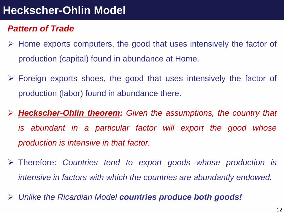
Pattern of Trade

Home exports computers, the good that uses intensively the factor of

production (capital) found in abundance at Home.

Foreign exports shoes, the good that uses intensively the factor of

production (labor) found in abundance there.

Heckscher-Ohlin theorem: Given the assumptions, the country that

is abundant in a particular factor will export the good whose

production is intensive in that factor.

Therefore: Countries tend to export goods whose production is

intensive in factors with which the countries are abundantly endowed.

Unlike the Ricardian Model countries produce both goods!

13


The first test of the Heckscher-Ohlin theorem was performed by

economist Leontief in 1953.

Leontief supposed correctly that in 1947 the United States was

abundant in capital relative to the rest of the world.

Thus, from the Heckscher-Ohlin theorem, Leontief expected that the

United States would export capital-intensive goods and import labor-

intensive goods.

What Leontief actually found, however, was just the opposite: the

capital–labor ratio for U.S. imports was higher than the capital–labor

ratio found for U.S. exports. This finding contradicted the Heckscher-

Ohlin theorem and came to be called Leontief’s paradox.

14


Leontief’s Paradox

Leontief used the numbers in this table to test the Heckscher-Ohlin

theorem. Each column shows the amount of capital or labor needed to

produce $1 million worth of exports from, or imports into, the United States

in 1947. As shown in the last row, the capital–labor ratio for exports was

less than the capital–labor ratio for imports, which is a paradoxical finding.

<

15


Leontief’s Paradox: Possible Explanations

U.S. and foreign technologies are not the same, in contrast to what

the HO theorem and Leontief assumed.

By focusing only on labor and capital, Leontief ignored land

abundance in the United States.

Leontief should have distinguished between skilled and unskilled labor

(because it would not be surprising to find that U.S. exports are

intensive in skilled labor).

The data for 1947 may be unusual because World War II had ended

just two years earlier.

The United States was not engaged in completely free trade, as the

Heckscher-Ohlin theorem assumes.

16


To determine whether a country is abundant in a certain factor, we compare the

country’s share of that factor with its share of world GDP (data for 2010).

If its share of a factor exceeds its share of world GDP, then we conclude that the

country is abundant in that factor.

If its share in a certain factor is less than its share of world GDP, then we conclude that

the country is scarce in that factor.

17


Differing Productivities Across Countries

In the original formulation of the paradox, Leontief had found that the

United States was exporting labor-intensive products even though it

was capital-abundant at that time.

One explanation for this outcome would be that labor is highly productive in

the United States and less productive in the rest of the world.

If that is the case, then the effective labor force in the United States, the

labor force times its productivity, is much larger than it appears to be when

we just count people.

To allow factors of production to differ in their productivities across

countries, we define the effective factor endowment as the actual

amount of a factor found in a country times its productivity.

Effective factor endowment = Actual factor endowment • Factor productivity

18


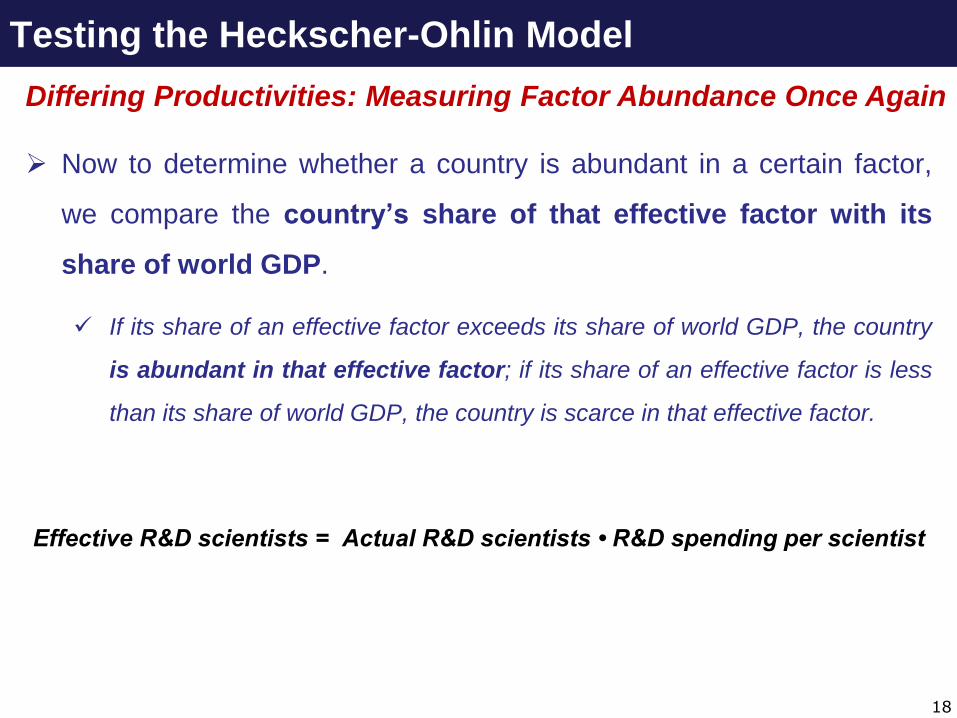
Differing Productivities: Measuring Factor Abundance Once Again

Now to determine whether a country is abundant in a certain factor,

we compare the country’s share of that effective factor with its

share of world GDP.

If its share of an effective factor exceeds its share of world GDP, the country

is abundant in that effective factor; if its share of an effective factor is less

than its share of world GDP, the country is scarce in that effective factor.

Effective R&D scientists = Actual R&D scientists • R&D spending per scientist

19


Adjusting the information from the previous Figure with the productivity of

each factor across countries we obtain the “effective” shares.

“Effective” Factor Endowments, 2010

20


Labor Endowment and GDP for the United States and Rest of World, 1947

Leontief’s Paradox Once Again: Labor Abundance

Shown here are the share of labor, “effective” labor, and GDP of the U.S. and the rest of

the world in 1947. The U.S. had only 8% of the world’s population, as compared to 37%

of the world’s GDP, so it was very scarce in labor. But when we measure effective labor

by the total wages paid in each country, then the US had 43% of the world’s effective

labor as compared to 37% of GDP, so it was abundant in effective labor.

21


Labor Productivity and Wages

Leontief’s Paradox Once Again: Labor Productivity

We expect this close connection between wages and labor productivity from the

Ricardian model, in which technology differences across countries determine wages,

and this is also what we expect to hold in the Heckscher-Ohlin model once we drop the

assumption of identical technologies.

22

Take a Break

23


Labor Productivity and Wages

Effect of Trade on the Wage and Rental of Home

The economy-wide relative demand for labor, RD, is an average of the LC /KC and LS /KS

curves and lies between these curves. The relative supply, L/K, is shown by a vertical

line because the total amount of resources in Home is fixed. The equilibrium point A, at

which relative demand RD intersects relative supply L/K, determines the wage relative

to the rental, W/R.

Relative

supplyRelative

demand

Relative demand of labor

in each sector

24

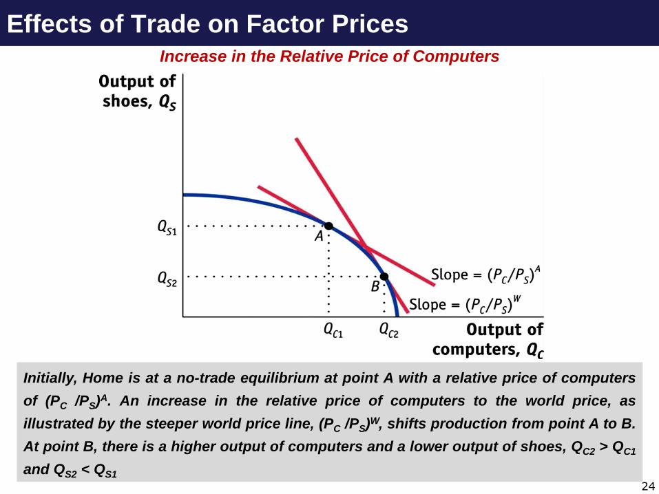
Effects of Trade on Factor PricesIncrease in the Relative Price of Computers

Initially, Home is at a no-trade equilibrium at point A with a relative price of computers

of (PC /PS)A. An increase in the relative price of computers to the world price, as

illustrated by the steeper world price line, (PC /PS)W, shifts production from point A to B.

At point B, there is a higher output of computers and a lower output of shoes, QC2 > QC1

and QS2 < QS1

25

Effects of Trade on Factor PricesEffect of a Higher Relative Price of Computers on Wage/Rental

An increase in the relative price of computers shifts the economy-wide relative demand

for labor, RD1, toward the relative demand for labor in the computer industry, LC /KC.

The new relative demand curve, RD2, intersects the relative supply curve for labor at a

lower relative wage, (W/R)2.

26

Effects of Trade on Factor PricesEffect of a Higher Relative Price of Computers on Wage/Rental

As a result, the wage relative to the rental falls from (W/R)1 to (W/R)2. The lower relative

wage causes both industries to increase their labor–capital ratios, as illustrated by the

increase in both LC /KC and LS /KS at the new relative wage.

27


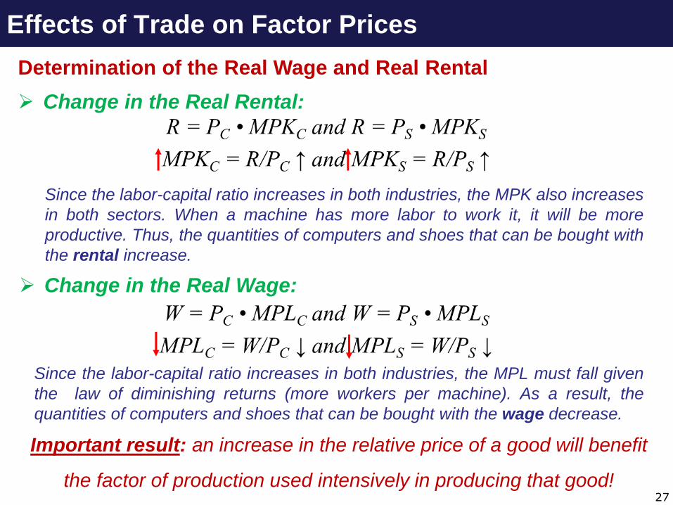
Determination of the Real Wage and Real Rental

Change in the Real Rental:

Change in the Real Wage:

Since the labor-capital ratio increases in both industries, the MPK also increases

in both sectors. When a machine has more labor to work it, it will be more

productive. Thus, the quantities of computers and shoes that can be bought with

the rental increase.

Since the labor-capital ratio increases in both industries, the MPL must fall given

the law of diminishing returns (more workers per machine). As a result, the

quantities of computers and shoes that can be bought with the wage decrease.

Important result: an increase in the relative price of a good will benefit

the factor of production used intensively in producing that good!

28

Effects of Trade on Factor Prices: Summarizing

Stolper-Samuelson Theorem

In the long run, when all factors are mobile, an increase in the

relative price of a good will increase the real earnings of the

factor used intensively in the production of that good and

decrease the real earnings of the other factor.

For our example, the Stolper-Samuelson theorem predicts

that when Home opens to trade and faces a higher relative

price of computers, the real rental on capital in Home rises

and the real wage in Home falls. In Foreign, the changes in

real factor prices are just the reverse.

In sum, in the HO model, the relatively abundant factor gains from

trade, while the scarce factor loses from trade.

29

Stolper-Samuelson theorem: A Numerical Example

How much the real wage and rental can change in response to a

change in price:

Computers:

Sales revenue = PC • QC = 100

Earnings of labor = W • LC = 50

Earnings of capital = R • KC = 50

where LC and KC is the amount of labor and capital used in the production to computers

Shoes:

Sales revenue = PS • QS = 100

Earnings of labor = W • LS = 60

Earnings of capital = R • KS = 40

where LS and KS is the amount of labor and capital used in the production of shoes

30


Notice that shoes are more labor-intensive than computers: the

share of total revenue paid to labor in shoes is 60/100 = 60%

and more than that share in computers is 50/100 = 50%.

When Home and Foreign undertake trade, the relative price of

computers rises in Home. For simplicity:

Computers: Percentage increase in price = ΔPC /PC = 10%

Shoes: Percentage increase in price = ΔPS /PS = 0%

31


The rental on capital can be calculated by taking total sales

revenue in each industry, subtracting the payments to labor, and

dividing by the amount of capital.

This calculation gives us the following formulas for the rental in

each industry:

Note that due to the factor

mobility, the rental is the

same in each industry

32


The price of computers has risen, so Δ PC > 0, holding fixed the

price of shoes, Δ PS = 0.

We can trace through how this affects the rental by changing PC

and W in the previous two equations:

33


It is convenient to work with percentage changes in the

variables. We can introduce these terms into the preceding

formulas by rewriting them as:

Plug the above data for shoes and computers into these

formulas:

34


Subtracting one equation from the other we get:

Simplifying the last line, we get

35


To find the change in the rental paid to capital (ΔR/R), we can

take our solution for ΔW/W = −40%, and plug it into the equation

for the change in the rental in the shoes sector.

36


The long-run results of a change in factor prices can be

summarized in the following equation:

The relationship between the changes in product prices to

changes in factor prices are called the “magnification effect”

because it shows how changes in the prices of goods have a

magnified effect on the earnings of factors

the heckscher-ohlin model · 3 introduction the heckscher-ohlin (ho) model, a model that assumes...

Documents