1. The Henyey-Greenstein phase function.

Henyey and Greenstein (1941) introduced a function which, by the variation of one

parameter, −1 ≤ g ≤ 1, ranges from backscattering through isotropic scattering to forward

scattering. The function is

p(θ) =1

4π

1 − g2

[1 + g2 − 2g cos(θ) ]3/2, (1)

This function is normalized such that the integral over 4π steradians is unity:∫

2π

0

{∫ π

0

p(θ) sin(θ) dθ

}

dφ = 1 (2)

We can write it as a function of µ = cos(θ) :

p(µ) =1

2

1 − g2

[1 + g2 − 2g µ ]3/2, and then

∫

1

−1

p(µ) dµ = 1 . (3)

Forward scattering is θ = 0, µ = 1, and in that case p(1) = (1 − g2)/2(1 − g)3, while for

back-scattering, θ = π, µ = −1, and p(−1) = (1 − g2)/2(1 + g)3. We see that the ratio of

forward to back scattering is [(1 + g)/(1 − g)]3. For g > 0, forward scattering is dominant,

while for g < 0, backscattering predominates.

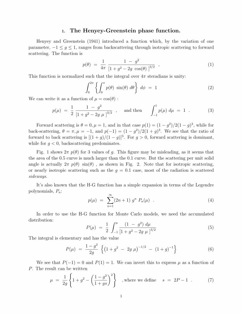
Fig. 1 shows 2π p(θ) for 3 values of g. This figure may be misleading, as it seems that

the area of the 0.5 curve is much larger than the 0.1 curve. But the scattering per unit solid

angle is actually 2π p(θ) sin(θ) , as shown in Fig. 2. Note that for isotropic scattering,

or nearly isotropic scattering such as the g = 0.1 case, most of the radiation is scattered

sideways.

It’s also known that the H-G function has a simple expansion in terms of the Legendre

polynomials, Pn:

p(µ) =∞

∑

n=1

(2n + 1) gn Pn(µ) . (4)

In order to use the H-G function for Monte Carlo models, we need the accumulated

distribution:

P (µ) =1

2

∫ µ

−1

(1 − g2) dµ

[1 + g2 − 2g µ ]3/2(5)

The integral is elementary and has the value

P (µ) =1 − g2

2g

{

(

1 + g2 − 2g µ)

−1/2 − (1 + g)−1

}

(6)

We see that P (−1) = 0 and P (1) = 1. We can invert this to express µ as a function of

P . The result can be written

µ =1

2g

{

1 + g2 −(

1 − g2

1 + gs

)2}

,where we define s = 2P − 1 . (7)

1

Fig. 1.— Polar plot of p(θ) for g = 0.1, green; g = 0.3, blue; g = 0.5, red.

2

Fig. 2.— Polar plot of p(θ) sin(θ) for g = 0.1, green; g = 0.3, blue; g = 0.5, red.

3

We see that as P varies from [0 → 1], s varies from [−1 → 1], and µ ranges from [−1 → 1]. If

we then replace P by some r drawn uniformly at random on the interval [0, 1], the distribution

of the values of µ will, for a large sample, approach the Henyey-Greenstein phase function.

Equation (7) breaks down at g = 0, but if we expand in powers of g, we see that

µ ≃ s +3

2g (1 − s2) − 2 g2 s(1 − s2) − · · · (8)

which approaches the isotropic result µ = s for g = 0.

Here is a J verb for the inverse of the accumulated H-G function:

NB. The inverse of the accumulated Henyey-Greenstein phase

NB. function. Run “g iAHG r” for random numbers r in

NB. the interval [0,1]; this gives a distribution of µ = cos(θ)’s

NB. over the range [-1,1], following the H-G function with parameter g.

iAHG=: 4 : 0

s=. 1+ +:y

a=. 1+ g2=. *: g=. x

if. 1e 5< |g do.

b=. *:(1-g2)%>:g*s

-: g%˜ a-b

else.

s2=. 1- *:s

s+ (1.5*g*s2)- +:g2*s*s2

end.

)

4

2. The Rayleigh scattering phase function.

Small particles and electrons may scatter light according to the Rayleigh phase function.

While such scattering will result in polarization, if we neglect polarization effects, we can

just write the phase function for the amplitude of the light scattered from an unpolarized

beam. This function is

R(µ) =3

8

(

1 + µ2)

,which is normalized:

∫

1

−1

R(µ) dµ = 1 . (9)

The accumulated function is seen to be

F (µ) =

∫ µ

−1

R(µ) dµ =1

2+

1

8µ

(

3 + µ2)

. (10)

We want to assign F (µ) = r, where r are random numbers over the interval [0,1], and

obtain the corresponding distribution in µ. Multiplying by 3, the equation we want to solve

is

µ3 + 3µ + 4(1 − 2r) = 0 (11)

which we write as

µ3 + 3µ − 2z = 0 where we have defined z = 2(2r − 1) . (12)

The solution of this cubic equation is our desired result:

µ = A + B ,where A =[

z +√

z2 + 1]1/3

and B =[

z −√

z2 + 1]1/3

. (13)

3. References.

Henyey, L.G., and Greenstein, J.L. (1941), Ap.J.,93, 70.

5

Fig. 3.— Polar plot of the Rayleigh phase function R(θ) = (3/8)[1 + cos2(θ)] .

6