The Hydrogen AtomThe Hydrogen AtomQuantum Physics2002

Recommended Recommended Reading:Reading:

Harris Chapter 6, Sections 3,4• Spherical coordinate system

•The Coulomb Potential•Angular Momentum• Normalised Wavefunctions•Energy Levels• Degeneracy

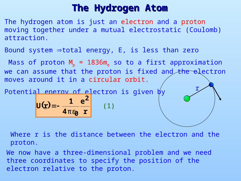
The Hydrogen AtomThe Hydrogen AtomThe hydrogen atom is just an electron and a proton moving together under a mutual electrostatic (Coulomb) attraction.

Bound system total energy, E, is less than zero

Mass of proton Mp = 1836me so to a first approximation we can assume that the proton is fixed and the electron moves around it in a circular orbit.

Potential energy of electron is given by

r

e4

1rU

2

0πε (1)

Where r is the distance between the electron and the proton.

r

We now have a three-dimensional problem and we need three coordinates to specify the position of the electron relative to the proton.

The Coulomb PotentialThe Coulomb Potential

r

U(r)

r

e4

1rU

2

0πε

Note that :

U(r) 0 as r

and

U(r) - as r 0

We want to find the wave functions and allowed energies for the electron when it is confined to this potential.

(2)

Spherical Coordinates (r,Spherical Coordinates (r,,,))

y

x

z

r

r sin

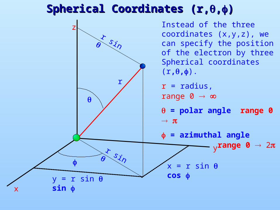
y = r sin sin

x = r sin cos

r sin

Instead of the three coordinates (x,y,z), we can specify the position of the electron by three Spherical coordinates (r,,).

r = radius, range 0

= polar angle range 0

= azimuthal anglerange 0 2

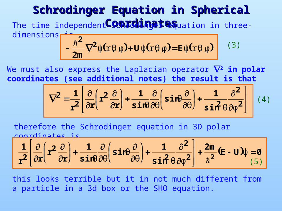
Schrodinger Equation in Spherical Schrodinger Equation in Spherical CoordinatesCoordinatesThe time independent Schrodinger equation in three-dimensions

is

φθ,r,ψφθ,r,ψφθ,r,ψ EUm2

22

We must also express the Laplacian operator 2 in polar coordinates (see additional notes) the result is that

2

2

22

22

sin

1sin

sin1

rr

rr

1

φθθθ

θθ

therefore the Schrodinger equation in 3D polar coordinates is

0UEm2

sin

1sin

sin1

rr

rr

122

2

22

2

ψφθθ

θθθ

this looks terrible but it in not much different from a particle in a 3d box or the SHO equation.

(3)

(4)

(5)

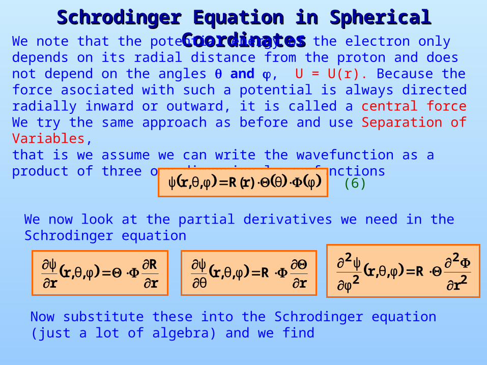
Schrodinger Equation in Spherical Schrodinger Equation in Spherical CoordinatesCoordinatesWe note that the potential energy of the electron only depends on

its radial distance from the proton and does not depend on the angles and , U = U(r). Because the force asociated with such a potential is always directed radially inward or outward, it is called a central force We try the same approach as before and use Separation of Variables, that is we assume we can write the wavefunction as a product of three one-dimensional wavefunctions

φθφθψ )r(R,,r

We now look at the partial derivatives we need in the Schrodinger equation

rR

,,rr

φθψ

rR,,r

φθθ

ψ 2

2

2

2

rR,,r

φθ

φ

ψ

Now substitute these into the Schrodinger equation (just a lot of algebra) and we find

(6)

0RUEm2

sinr

R

sinsinr

RrR

rrr

22

2

22

22

2

φθ

θθ

θθ

Multiply across by r2sin2 and divide across by R.. and rearrange:

2

2222

2 1 UEsinr

m2sin

sinrR

rrR

sin2 φ

θθ

θθ

θθ

On the left hand side we have only functions of r and , while the right hand side is only a function of , (Separation of Variables) This can only hold for all values of r, and if both sides are equal to a constant. We call this constant mL

2.

Then taking the R.H.S. we have 0m m

1 2

L2

22L2

2

φφ

The the azimuthal equation describes how the wavefunction varies with angle and are the azimuthal wave functions. This is the same equation as that for a Particle on a Ring and Sphere which we solved previously.

(7)

(8)

(9)

2L

2222

m UEsinrm2

sinsin

rR

rrR

sin2

θ

θθ

θ

θθ

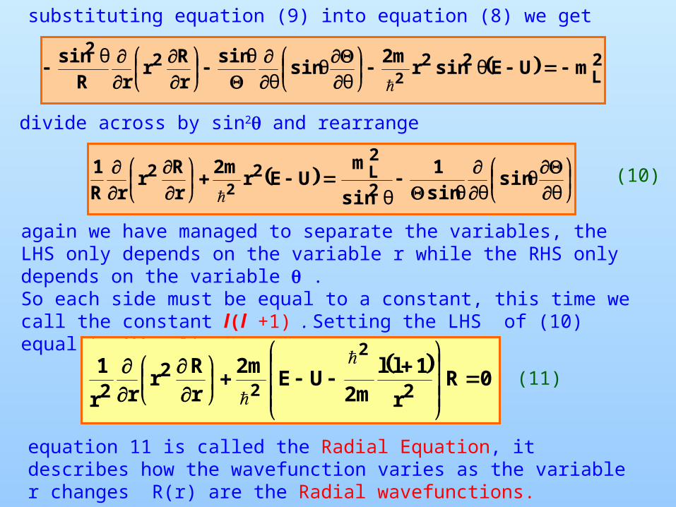
substituting equation (9) into equation (8) we get

(10)

divide across by sin2 and rearrange

θθ

θθθsin

sin1

sin

m UEr

m2rR

rrR

12

2L22

2

again we have managed to separate the variables, the LHS only depends on the variable r while the RHS only depends on the variable .So each side must be equal to a constant, this time we call the constant l(l +1) . Setting the LHS of (10) equal to l(l + 1) gives

0 R

r

1l lm2

UEm2

rR

rrr

1

22

2

2

2

(11)

equation 11 is called the Radial Equation, it describes how the wavefunction varies as the variable r changes R(r) are the Radial wavefunctions.

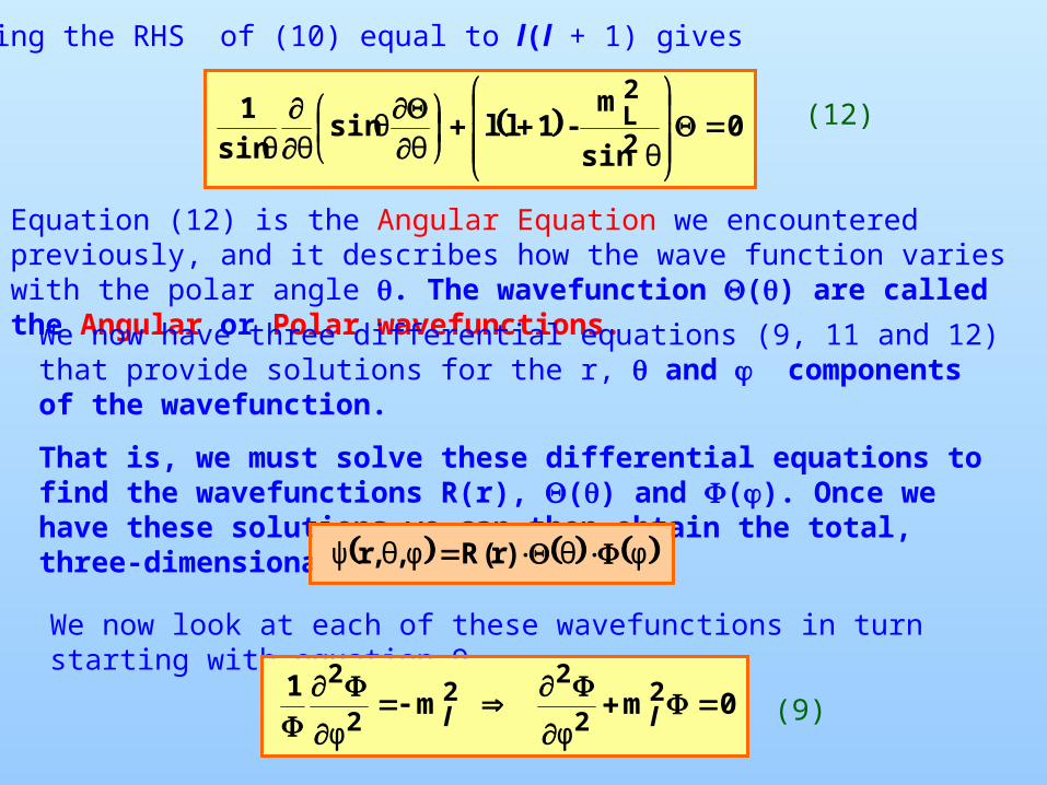
Setting the RHS of (10) equal to l(l + 1) gives

0sin

m- 1l lsin

sin1

2

2L

θθθ

θθ(12)

Equation (12) is the Angular Equation we encountered previously, and it describes how the wave function varies with the polar angle . The wavefunction () are called the Angular or Polar wavefunctions.We now have three differential equations (9, 11 and 12) that

provide solutions for the r, and components of the wavefunction.

That is, we must solve these differential equations to find the wavefunctions R(r), () and (). Once we have these solutions we can then obtain the total, three-dimensional wavefunction from

We now look at each of these wavefunctions in turn starting with equation 9

0m m1

22

22

2

2

ll

φφ(9)

φθφθψ )r(R,,r

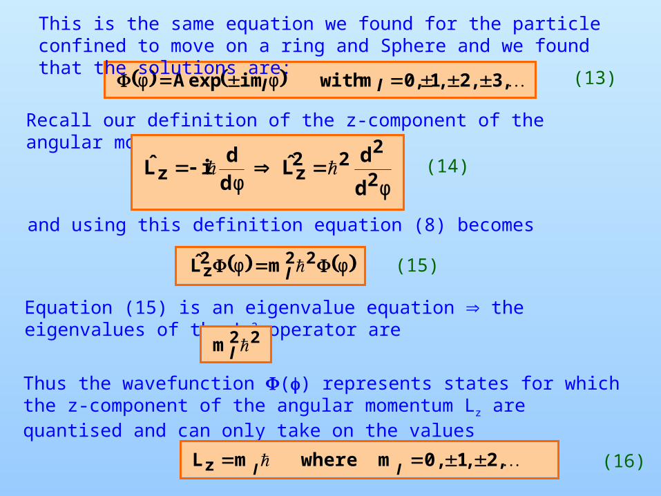
,3 ,2 ,1,0m with imexpA llφφ

This is the same equation we found for the particle confined to move on a ring and Sphere and we found that the solutions are:

Recall our definition of the z-component of the angular momentum operator

φφ 2

222

zzd

dL̂

dd

iL̂

(13)

(14)

and using this definition equation (8) becomes

φφ 222z mL̂ l (15)

Equation (15) is an eigenvalue equation the eigenvalues of the Lz

2 operator are 22m l

Thus the wavefunction () represents states for which the z-component of the angular momentum Lz are quantised and can only take on the values

,2 ,1 0,m where mLz ll (16)

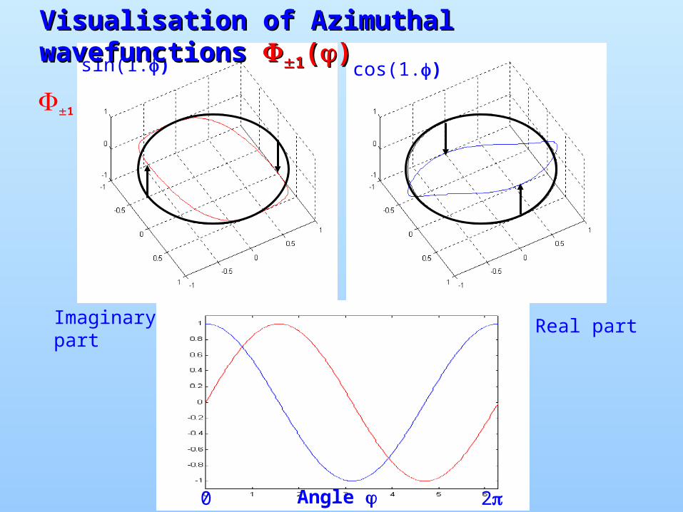
sin(1.) cos(1.)

1

Visualisation of Azimuthal Visualisation of Azimuthal wavefunctionswavefunctions 11(())

0 2

Angle

Imaginary part

Real part

sin(1.) cos(1.)

1

Imaginary part

Real part

--

++

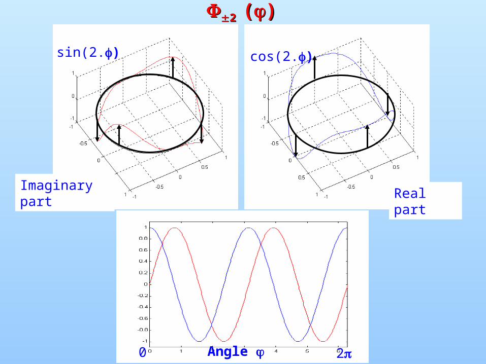
sin(2.) cos(2.)

2 2 (())

0 2

Angle

Imaginary part

Real part

22

+

+++

-

-

-

-

Imaginary part

Real part

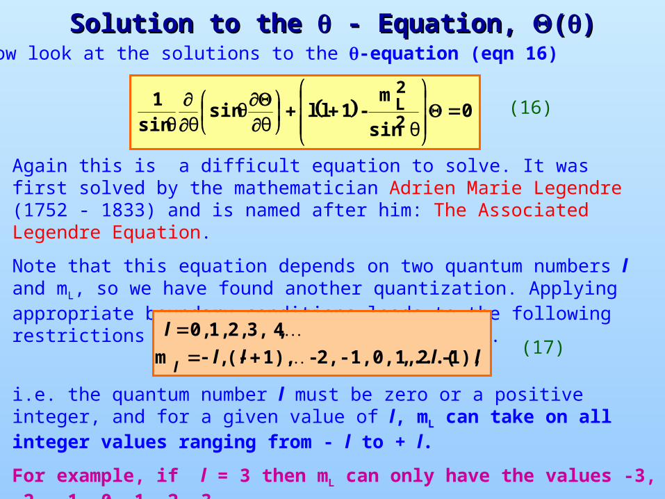
Solution to the Solution to the - Equation, - Equation, (())We now look at the solutions to the -equation (eqn 16)

0sin

m- 1l lsin

sin1

2

2L

θθθ

θθ

Again this is a difficult equation to solve. It was first solved by the mathematician Adrien Marie Legendre (1752 - 1833) and is named after him: The Associated Legendre Equation.

Note that this equation depends on two quantum numbers l and mL, so we have found another quantization. Applying appropriate boundary conditions leads to the following restrictions on the quantum numbers l and mL.

llll

l

l1),-,...(2,-1,0,1,2- 1),(- ,m

, 43, 2, 1, 0,

i.e. the quantum number l must be zero or a positive integer, and for a given value of l, mL can take on all integer values ranging from - l to + l.

For example, if l = 3 then mL can only have the values -3, -2, -1, 0, 1, 2, 3

(16)

(17)

What are the solutions of the The Associated Legendre Equation?The solutions are a called the Associated Legendre Functions, Pl,mL(cos ) they are polynomials that depend on the angle and the two quantum numbers l and ml. For each allowed set of quantum numbers (l, mL) there is a solution l,mL(). The first few are given in the following table

l mL Pl,mL(cos )0 0 11 0 cos 1 1 sin 2 0 (3cos2 - 1)/22 1 3cos sin 2 2 3sin2

l mL Pl,mL(cos )3 0 (5cos3 - 3cos)/23 1 3sin(5cos2 -1)/23 2 15cossin23 3 15sin3

the solutions to the angular equation are given byl,mL

() = Pl,mL(cos )

What do these wavefunctions look like? Exactly the same as a particle on a sphere. Let us plot a few of them

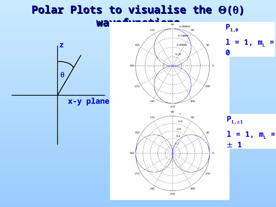
Polar Plots to visualise the Polar Plots to visualise the (() ) wavefunctionswavefunctions

z

x-y plane

P1,0

l = 1, mL = 0

x-y plane

P1,1

l = 1, mL = 1

P2,0

l = 2, mL = 0

P2,1

l = 2, mL = 1

P2,1

l = 2, mL = 2

P3,0

l = 3, mL = 0

P3,1

l = 3, mL = 1

P3, 2

l = 3, mL = 2

P3, 3

l = 3, mL = 3

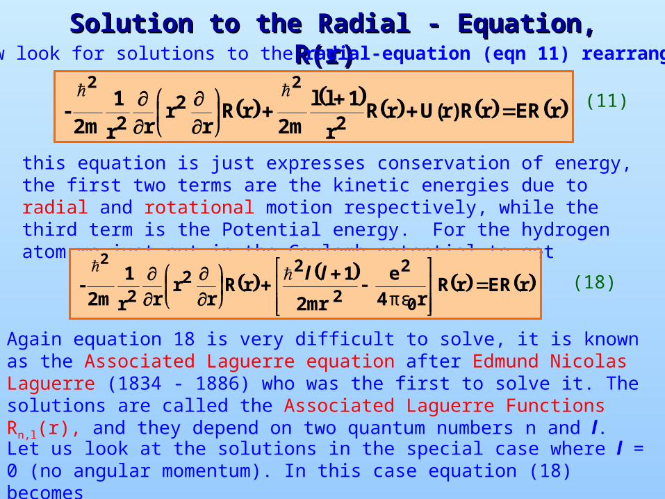
Solution to the Radial - Equation, R(r) Solution to the Radial - Equation, R(r) We now look for solutions to the radial-equation (eqn 11) rearranged as

rER rR )r(UrRr

1l lm2

rRr

rrr

1m2

- 2

22

22

(11)

this equation is just expresses conservation of energy, the first two terms are the kinetic energies due to radial and rotational motion respectively, while the third term is the Potential energy. For the hydrogen atom we just put in the Coulomb potential to get

rER rR r4

e

mr2

1 rR

r

rrr

1m2

- 0

2

2

22

2

2

πε

ll(18)

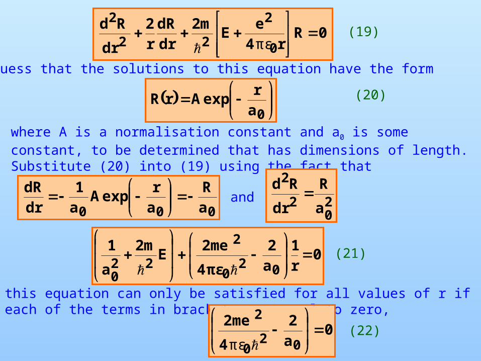
Again equation 18 is very difficult to solve, it is known as the Associated Laguerre equation after Edmund Nicolas Laguerre (1834 - 1886) who was the first to solve it. The solutions are called the Associated Laguerre Functions Rn,l(r), and they depend on two quantum numbers n and l. Let us look at the solutions in the special case where l = 0 (no angular momentum). In this case equation (18) becomes

0R r4

eE

m2drdR

r2

dr

Rd

0

2

22

2

πεwe guess that the solutions to this equation have the form

0ar

expArR (20)

(19)

where A is a normalisation constant and a0 is some constant, to be determined that has dimensions of length. Substitute (20) into (19) using the fact that

000 aR

ar

expAa1

drdR

and 2

02

2

a

R

dr

Rd

0r1

a2

πε4

2meE

m2

a

1

020

2

220

(21)

this equation can only be satisfied for all values of r if each of the terms in brackets are equal to zero,

0a2

4

2me

020

2

πε(22)

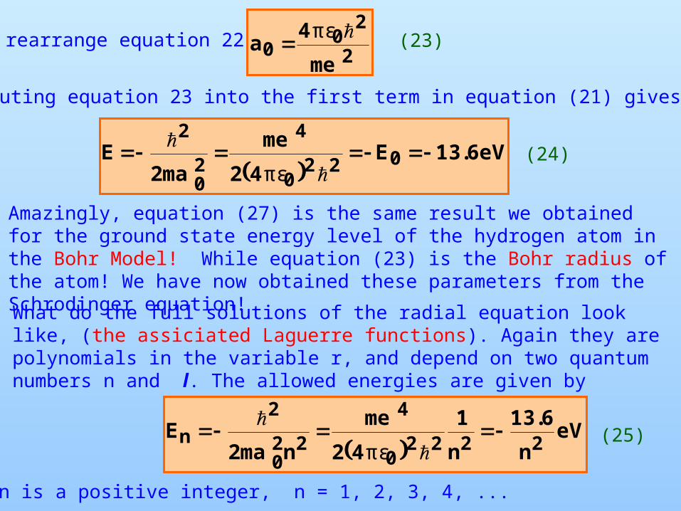
rearrange equation 22 2

20

0me

4a

πε (23)

substuting equation 23 into the first term in equation (21) gives

eV6.13E

42

me

ma2E 022

0

4

20

2

πε(24)

Amazingly, equation (27) is the same result we obtained for the ground state energy level of the hydrogen atom in the Bohr Model! While equation (23) is the Bohr radius of the atom! We have now obtained these parameters from the Schrodinger equation!

What do the full solutions of the radial equation look like, (the assiciated Laguerre functions). Again they are polynomials in the variable r, and depend on two quantum numbers n and l. The allowed energies are given by

eV

n

6.13

n

1

42

me

nma2E

22220

4

220

2n

πε

where n is a positive integer, n = 1, 2, 3, 4, ...

(25)

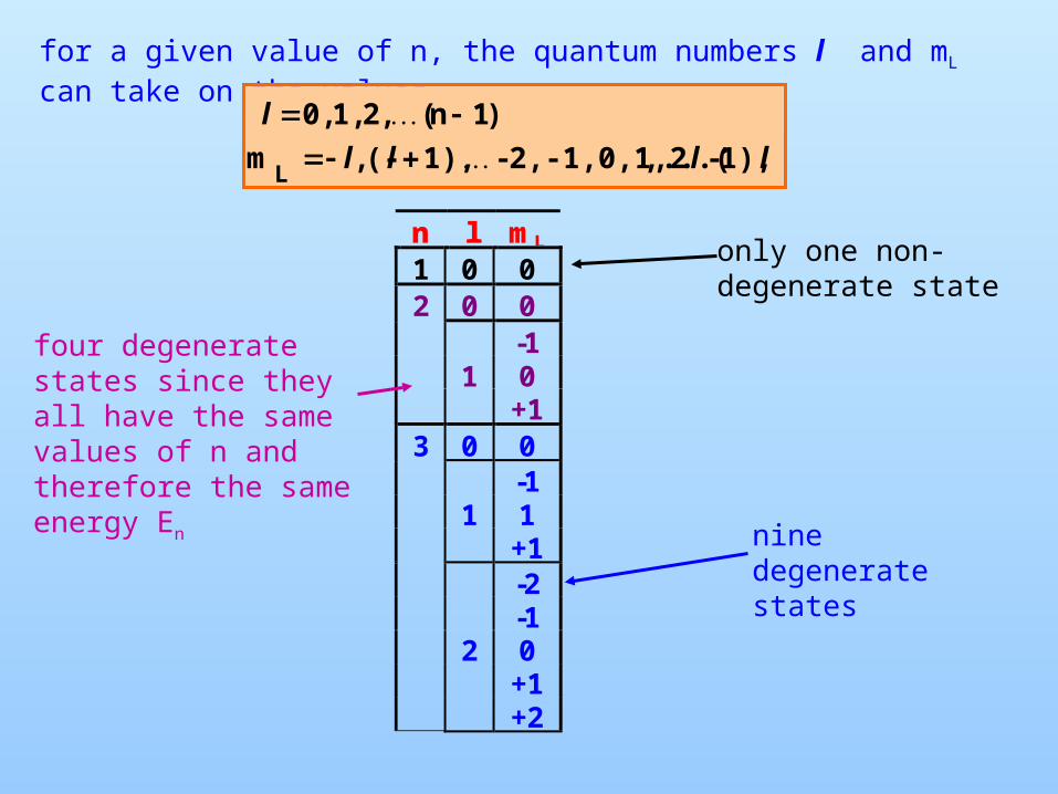
for a given value of n, the quantum numbers l and mL can take on the values

llll

l

1),-,...(2,-1,0,1,2- 1),(- ,m

)1n( ,2 1, 0,

L

n l mL

1 0 02 0 0

-11 0

+13 0 0

-11 1

+1-2-1

2 0+1+2

only one non-degenerate state

four degenerate states since they all have the same values of n and therefore the same energy En

nine degenerate states

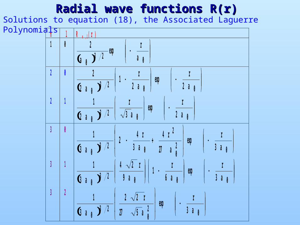
Radial wave functions R(r) Radial wave functions R(r)

n l R n , l ( r )1 0

0230 a

rexp

a

2

2 0

00230 a2

rexp

a2r

1a2

2

2 1

00230 a2

rexp

a3r

a2

1

3 0

020

2

0230 a3

rexp

a27

r4a3

r42

a3

1

3 1

000230 a3

rexp

a6r

1a9

r 24

a3

1

3 2

020

230 a3

rexp

a527

r 22

a3

1

Solutions to equation (18), the Associated Laguerre Polynomials

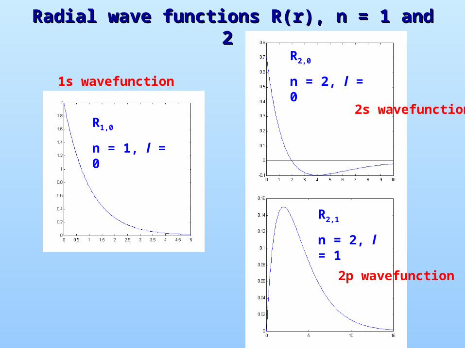
Radial wave functions R(r), n = 1 and 2 Radial wave functions R(r), n = 1 and 2

R1,0

n = 1, l = 0

R2,0

n = 2, l = 0

R2,1

n = 2, l = 1

1s wavefunction

2s wavefunction

2p wavefunction

R3,0

n = 3, l = 0

R3,1

n = 3, l = 1

R3,2

n = 3, l = 2

Radial wave functions R(r) for n = 3Radial wave functions R(r) for n = 33s wavefunction 3p wavefunction

3d wavefunctionSince there is no upper limit to the value n can have, there are an infinite number of radial wavefunctions, but they all have finite energies En