the iasb insurance project for life insurance contracts: impact on reserving …€¦ · ·...
TRANSCRIPT

Faculty of Actuarial Science and Statistics
The IASB Insurance Project for life insurance contracts: impact on reserving methods and solvency requirements.
Laura Ballotta, Giorgia Esposito and Steven Haberman.
Actuarial Research Paper No. 162 May 2005 ISBN 1-901615-86-3
Cass Business School 106 Bunhill Row London EC1Y 8TZ T +44 (0)20 7040 8470 www.cass.city.ac.uk
Cass means business

“Any opinions expressed in this paper are my/our own and not necessarily those of my/our employer or anyone else I/we have discussed them with. You must not copy this paper or quote it without my/our permission”.

The IASB Insurance Project for life insurancecontracts: impact on reserving methods and solvency
requirements
Laura Ballotta∗, Giorgia Esposito†, Steven Haberman‡
May 26, 2005
Abstract
In this communication, we review the fair value - based accounting frameworkpromoted by the IASB Insurance Project for the case of a life insurance com-pany. In particular, by means of a simple participating contract with minimumguarantee, we compare the fair value approach with the “traditional” account-ing system based on the construction of mathematical reserves, and we assessthe adequacy of the two reporting frameworks in terms of covering of the lia-bility, implementation cost, volatility of reported earnings and solvency capitalrequirements.
Keywords: Black-Scholes option pricing formula, fair value, Levy processes,mathematical reserves, participating contracts, shortfall probability, solvency re-quirements.
1 Introduction
In response to an increasingly difficult economic climate, in which the financial stabilityof the insurance industry has been affected by events such as the crash in the equitymarkets in 2001 and 2002, a steady fall in bonds yields, as well as increased longevity,the focus of regulators on accounting rules, capital adequacy and solvency requirementsfor insurance companies has increased.
In particular, the three common themes behind the activity of many regulatorybodies around the world are a comprehensive financial reporting framework for theappropriate assessment of the specific risks that insurance companies are running;
∗Faculty of Actuarial Science and Statistics, Cass Business School, City University London, e-mail:[email protected].
†Department of Actuarial and Financial Sciences, University of Rome La Sapienza, e-mail: [email protected]
‡Faculty of Actuarial Science and Statistics, Cass Business School, City University London, e-mail:[email protected].
1

the standardization of approaches between countries and industries, where sensible;and an improved transparency and comparability of accounting information. To thispurpose, the International Accounting Standards Board (IASB) in Europe and theFinancial Accounting Standards Board (FASB) in the US have been working over thelast few years towards the proposal of a model for the valuation of assets and liabilitieswhich produces comparable, reliable and market consistent measurements. As such,the focus of this model has to be on the “economic” value of the insurance companiesbusiness. This theme has been followed by IASB and FASB with the proposal of a “fairvalue” accounting system for all assets and liabilities, where by fair value it is meant“the amount for which an asset could be exchanged, or a liability settled, betweenknowledgeable, willing parties in an arm’s length transaction” (IASB, 2004).
In Europe, phase 1 of the IASB Insurance Project has been completed with the is-suance of the new International Financial Reporting Standard (IFRS) 4 in March 2004,which establishes the changes in accounting rules as of January 2005. It is not our aimto describe here the technicalities of the new IFRS 4 (for a comprehensive exposition ofits main features, we refer for example to FitchRatings, 2004). However, we note thatphase 1 requires significantly increased disclosure of accounting information, but onlyrelatively limited changes to the accounting methodology, as the majority of the liabili-ties that have to be recorded at fair value are those originated by derivatives embeddedin insurance contracts, such as life products offering a guarantee of minimum equityreturns on surrender or maturity. The changes to the treatment of the assets side ofthe balance sheet is, instead, the direct result of the implementation of IAS 39, underwhich investments have to be classified as “available for sale” or “held for trading”,and hence marked to market, unless the insurer is able to demonstrate the intent toforego future profit opportunities generated by these financial instruments (in whichcase investments can be classified as “held to maturity” and consequently reported atamortised historic cost). Hence, these changes are to be considered as the basis forthe transition period leading up to the proper fair value accounting framework, whichwill be implemented in phase 2 (expected at the time of writing) to be completed by2007-2008. We note, however, that the regulatory bodies in the UK, the Netherlandsand Switzerland have introduced, or are in the process of introducing from January2006, accounting rules based on the full mark-to-market of assets and liabilities, to beaccompanied by the assessment of risk capital on a number of relevant adverse sce-narios. In particular, the Swiss Solvency Tests (FOPI, 2004) developed by the SwissFederal Office of Private Insurance, and the Twin Peaks/Individual Capital AdequacyStandard implemented by the Financial Service Authority in the UK (FSA, 2004) aredesigned to offer compatibility with regulatory demands on other market players likebanks.
In the financial literature, the topic of market consistent valuation of life insuranceproducts is well known and goes back to the work of Brennan and Schwartz (1976) onunit-linked policies. Since then, a wide range of contributions have followed, specifi-cally on the issue of the fair valuation of the different contract typologies available inthe insurance markets around the world (for a comprehensive review of these studies,we refer for example to Jørgensen (2004) and the references therein). However, it is
2

recognised that the adoption of the fair value approach in the financial reporting sys-tem may have a significant impact on the design of some life insurance products; thepremia charged to policyholders; the methodologies for the construction of reserves;and, more generally, the solvency profiles of companies. Hence, the purpose of thispaper is to analyze some of these aspects by means of a simple participating contractwith a minimum guarantee. In particular, we consider the effect of the fair valuationapproach on the default probability of the life insurance company issuing the contract.We note that no specific recommendation has yet been made by IASB as to whichstochastic model is the most appropriate as the target accounting model; hence, weadopt the standard Black-Scholes framework as a benchmark and, at the same time, wealso analyze the model risk and the parameter risk arising from this approach. Finally,we explore some possible alternative schemes for the construction of the mathematicalreserves, and consider the advantages of adopting the fair value approach for solvencyassessment purposes. Our focus on this last aspect is because of the ongoing EU Sol-vency II review of insurance firm’s capital requirements, which is expected to comeinto effect at the same time as phase 2 of the IASB Insurance Project.
The paper is organized as follows. In section 2, we describe the design of the sim-ple life insurance policy and the approach to fair valuation that we are considering inthis paper. The valuation approach leads to a fair premium for the contract. We alsodiscuss the extra premium that needs to be charged as a solvency loading to cover theinsurance company’s default option. In section 3, we propose a methodology for theanalysis of the model error and the parameter error components of the Market ValueMargin, as requested by the IASB. In sections 4 and 5, we provide a comparative studyof the performance of the fair valuation method. We propose a range of determinis-tic reserving methods (static and dynamic) for comparison with the fair value of theliability in section 4. In section 5, we introduce the concept of Risk Bearing Capital(RBC) and use this as a means of assessing the solvency of the insurance company.Section 6 provides some concluding comments.
2 The participating contract and market consistent
valuation
In this section, we consider a participating contract with a minimum guarantee and asimple mechanism for the calculation of the reversionary bonus. Following the generalrecommendation from the IASB accounting project, we then calculate the fair value ofthis contract using a stochastic model to represent the market dynamics of the fundbacking the policy. In particular, we choose as valuation framework the traditionalBlack and Scholes (1973) model; we also focus on the implication of the fair valuationprocess on the insurer’s solvency and on the definition of the contract premium. In theremaining parts of this paper we ignore lapses, mortality and any further benefit thatthe policyholder may receive from the participating contract, such as death benefits ora terminal bonus.
3

2.1 Fair valuation
Consider as given a filtered probability space(Ω,F , Ftt≥0 , P
), and let us assume that
the financial market is frictionless with continuous trading (i.e. there are no taxes, notransaction costs, no restrictions on borrowing or short sales and all securities areperfectly divisible). Furthermore, let r ∈ R
++ be the risk-free rate of interest.The policyholder enters the contract at time 0 paying an initial single premium P0,
which is invested by the insurance company in an equity fund, A. This is assumed tofollow the traditional geometric Brownian motion
dA (t) = µA (t) dt + σA (t) dW (t) , (1)
under the real objective probability P. The parameters µ ∈ R and σ ∈ R++ represent
respectively the expected rate of growth (i.e. the expected rate of return) and thevolatility of the fund.
In return, the policyholder receives a benefit, P , which accumulates annually atrate rP (t), so that
P (t) = P (t − 1) (1 + rP (t)) t = 1, 2, ..., T, (2)
with
P (0) = P0;
rP (t) = max
rG, β
(A (t) − A (t − 1)
A (t − 1)
).
The parameter β represents the participation rate of the policyholder in the returnsgenerated by the reference portfolio, whilst rG denotes the fixed guaranteed rate. Weassume that the policyholder receives the benefit only at maturity, T ; however, if atmaturity, the insurance company is not capable of paying the full amount P (T ), thenthe policyholder seizes the assets available. Hence, the liability, L, of the insurancecompany at maturity is
L (T ) =
A (T ) if A (T ) < P (T )P (T ) if A (T ) > P (T )
,
or, equivalentlyL (T ) = P (T ) − D (T ) , (3)
whereD (T ) = (P (T ) − A (T ))+
is the payoff of the so-called default option.From standard contingent claim theory, it follows that the market value at time
t ∈ [0, T ] of the participating contract is
VC (t) = E[e−r(T−t) (P (T ) − D (T ))
∣∣ Ft
](4)
= E[e−r(T−t)P (T )
∣∣ Ft
] − E[e−r(T−t)D (T )
∣∣ Ft
]= VP (t) − VD (t)
4

where E denotes the expectation under the risk-neutral probability measure P, and Ft
is the information flow up to (and including) time t.1
Given our set of assumptions, and the features of the policy design, a closed-formanalytical formula for the value of the policy reserve VP (t) can be obtained. Thesame, however, does not apply for the value of the default option, VD (t), due tothe recursive substitution of P and the fact that P is highly dependent on the pathfollowed by the reference fund A. Therefore, the market price of the default option willbe approximated by numerical procedures.
In more detail, from equation (2) it follows that
P (T ) = P0
t∏k=1
(1 + rP (k))T∏
k=t+1
(1 + rP (k)) = P (t)T−t∏j=1
(1 + rP (j)) .
Moreover,
rP (t) = max
rG, β
(A (t) − A (t − 1)
A (t − 1)
)= rG +
(β
(A (t) − A (t − 1)
A (t − 1)
)− rG
)+
= rG +
(β
(e
(µ−σ2
2
)+σW1 − 1
)− rG
)+
under P,
= rG +
(β
(e
(r−σ2
2
)+σW1 − 1
)− rG
)+
under P,
where W is a standard one-dimensional Brownian motion under the risk neutral proba-bility measure P. This implies that the annual rate of return rP (t) generates a sequenceof independent random variables ∀t ∈ [0, T ]. Therefore, the market value of the policyreserve is
VP (t) = P (t) E
[e−r(T−t)
T−t∏j=1
(1 + rP (j))
∣∣∣∣∣ Ft
]
= P (t)T−t∏j=1
E
e−r
[1 + rG +
(β
(e
(r−σ2
2
)+σW1 − 1
)− rG
)+]
= P (t)[e−r (1 + rG) + βN (d1) − e−r (β + rG) N (d2)
]T−t(5)
where
d1 =ln β
β+rG+
(r + σ2
2
)σ
; d2 = d1 − σ.
The pricing equation (5) follows as an application of the Black-Scholes option formula(see also Bacinello, 2001, Ballotta, 2005, and Miltersen and Persson, 2003, for similarresults).
1Note that we implicilty assume the existence of the risk-neutral probability measure P (which,given the specification of the market is unique). In other words, we assume that the participatingpolicy is attainable and therefore the replicating portfolio exists. This is consistent with the spirit ofFASB recognition of Level 3 fair value estimates for insurance liabilities with complex contingenciesand embedded options elements (FASB, 2004).
5

Fair value of the participating contractP0 VC (0) VP (0) VD (0)100 100 222.73 122.73
Relative solvency loading coefficient δ = 1.2273
Table 1: The fair value of the participating contract with minimum guarantee for the bench-mark set of parameters. The Monte Carlo simulation for the price of the default option isbased on 10,000 paths; the antithetic variate technique and the control variate method areused for variance reduction purposes.
2.2 Default probability and the premium for the participatingcontract
Based on the valuation formula (5), in this section we implement a scenario generationprocedure to analyze the evolution of the market value of the participating contractand the reference fund over the lifetime of the policy. Since these quantities representthe liabilities and the assets in the balance sheet of the insurer, this study will allowus to understand the consequences of the market based accounting standards on thesolvency profile of the life insurance.
The numerical procedure is organised in the following steps:
1. using the P-dynamic of the underlying asset A, we generate possible trajectoriesof the reference fund from the starting date of the policy till time t ∈ (0, T ]. Eachtrajectory consists of 1 observation per month.
2. Then, we calculate the annual returns on the reference fund A to obtain theamount accumulated by the policy till time t, P (t).
3. The output from step 2 is used to calculate VP (t) according to equation (5).
4. Finally, we use the output from step 1 and 2 to compute the market value of thedefault option, VD (t), using Monte Carlo methods. The Monte Carlo experimentis based on 10,000 paths; antithetic variate methods and the control variateprocedure are implemented in order to reduce the error of the estimates.
Unless otherwise stated, the initial single premium is P0 = 100 and the set ofparameters is as follows:
µ = 10% p.a.; σ = 15% p.a.; β = 80%; rG = 4% p.a.; r = 4.5% p.a.; T = 20 years.
The no arbitrage values of the contract and its components corresponding to theabove set of parameters are shown in Table 1; we note that, for the given set ofparameters, the premium charged to the policyholders satisfies the condition
P0 = VC (0) = VP (0) − VD (0) . (6)
This is consistent with the no arbitrage principle.
6

A possible scenario resulting from this numerical experiment is illustrated in Figure1.(a). In this plot, we show the evolution of the reference fund A, the fair value of thebenefit VP , the value of the default option VD, and the total value of the contract VC .We note that the assets of the life insurance company are not enough to guarantee thepayment of the full benefit promised at maturity; consequently, the curves representingthe assets’ price and the total value of the contract coincide (see equation (4)). Thedefault probability arising from this model, calculated on the basis of 100,000 scenarios,is in fact 74.42% (see Table 2).
The reason for such a high default risk can be found in the default option premium,VD. As equation (6) shows, the policy reserve is not the only component affecting thevalue of the participating contract, as we need also to take account of the fact that theinsurance company’s liability is limited by the market value of the reference fund. Thisfeature is captured by the payoff of the so-called default option D. Consequently, VD is,as Ballotta et al. (2005) observe, an estimate of the market loss that the policyholderincurs if a shortfall occurs. However, equation (6) also implies that
P0 + VD (0) = VP (0) .
Hence, as already observed by Ballotta (2005), the value VD of the default option canbe considered as the extra premium that the insurer has to charge the policyholderfor no arbitrage opportunities to arise. Without receiving this extra amount, in fact,the insurer would be offering the guaranteed benefits too cheaply, as the solvency riskattached to the contract would be ignored.
Based on these considerations, we redefine the overall premium paid by the policy-holder at inception of the contract to be P ′
0 = P0 + VD (0), where P0 is the part of thepremium on which the benefit will be based, and VD is instead the part of the premiumthat the policyholder has to pay in order to be “insured” against a possible default ofthe insurance company. In this sense, the fair value of the default option associated tothe participating contract, VD (0), could be regarded as a solvency, or safety, loadingto the premium. If we write VD (0) = δP0, then P ′
0 = (1 + δ) P0, with δ representing arelative solvency loading coefficient (Daykin et al. (1994)). If this additional premiumis invested in the market to purchase another share of the reference portfolio, at timet = 0, the value of the fund backing the policy is A (0) = P0, whilst the total valueof the assets available to the insurer is Atot (0) = P ′
0 = P0 + VD (0). Both A and Atot
evolve as described in equation (1).The dynamics of each component of the contract resulting from this readjustment
and corresponding to the scenario presented in Figure 1.(a), are illustrated in Figure1.(b). If the insurance company invests the additional premium in the same fundbacking the policy, the default option moves out of the money, whilst the value ofthe contract converges to the value of the promised benefits. The probability of ashortfall occurring at maturity is 6.97% as reported in Table 2 (on the basis of 100,000scenarios). Panels (a) and (c) of Figure 2 show the corresponding shortfall distributionfor both situations, i.e. when the premium for the default option is ignored (panel (a)),and when instead it is charged and invested in the fund (panel (c)). The reduction inthe right-tail of the distribution in the latter case is evident.
7

0 5 10 15 200
100
200
300
400
500
600
700
800
A(t)
VP(t)
VD
(t)
VC
(t)
time (years)
a) Geometric Brownian motion model: VD
(0) not charged
0 5 10 15 200
200
400
600
800
1000
1200 Atot
(t)
VP(t)
VD
(t)
VC
(t)
time (years)
b) Geometric Brownian motion model: VD
(0) charged and invested
0 5 10 15 200
100
200
300
400
500
600
700
S(t)
VP(t)
VD
(t)
VC
(t)
time (years)
c) Geometric Levy process model: VD
(0) not charged
0 5 10 15 200
100
200
300
400
500
600
700
800 Stot
(t)
VP(t)
VD
(t)
VC
(t)
d) Geometric Levy process model: VD
(0) charged and invested
time (years)
0 5 10 15 200
100
200
300
400
500
600
700
800
S(t)
VP(t)
VD
(t)
VC
(t)
time (years)
e) Geometric Levy process model: VD
(0) not charged
0 5 10 15 200
200
400
600
800
1000
1200
Stot
(t)
VP(t)
VD
(t)
VC
(t)
f) Geometric Levy process model: VD
(0) charged and invested
time (years)
Figure 1: Scenario generation: a possible evolution of the reference fund and the fair valueof the participating contract, the benefits and the default option. Panels (a)-(b) show onepossible scenario under the geometric Brownian motion paradigm presented in section 2.1.Panels (c)-(d) and (e)-(f) illustrate two possible scenarios under the Levy process paradigmdiscussed in section 3.1. The scenario generation has been obtained for the benchmark set ofparameters under the real probability measure P.
8

Probability of default at maturityGBM model P (P (T ) > A (T )) = 74.42% P (P (T ) > Atot (T )) = 6.97%GLP model P (P (T ) > S (T )) = 81.71% P (P (T ) > Stot (T )) = 12.74%
Table 2: Default probability at maturity under the geometric Brownian motion frameworkpresented in section 2.1 and the Levy process framework introduced in section 3.1. Calcu-lations have been performed for the benchmark set of parameters under the real probabilitymeasure, on the basis of 100,000 simulations.
3 Market value margin
The valuation model presented in the previous section, and therefore also the resultsdiscussed in section 2.2, relies on a number of assumptions (most notably, the assump-tion that the equity assets follow a log-normal distribution), and the specification of anumber of external variables, like the expected return of the assets or their volatility,that can move significantly over the lifetime of the contract. It is widely acknowledgedthat it is difficult to classify accurately the distribution of market prices and to assessthe probability of extreme events, especially falls, concerning stock prices. This impliesthat, as discussed in Ballotta (2005), there are biases in the fair value measurementsoriginating from the model developed in the previous section.
The aim of this part of the paper is to examine the impact of this type of uncertainty,affecting the fair valuation of insurance liabilities, on the expected cash flows and thesolvency profile of the insurer. We note that the IASB intends to take into accountthese elements of risk, the so-called model risk and parameter risk, during phase 2 of theimplementation of the accounting standards project, by requiring insurance companiesto calculate a Market Value Margin (see, for example, FitchRatings, 2004) as a bufferto reflect the risks and uncertainties that are inherent in insurance contracts.
3.1 The model error
As previously mentioned, the calculations of fair values presented in section 2 aredependent on the assumption of normal distributed log-returns. However, it is wellknown that, in the real financial market, this is not the case, as the dynamic of theassets is not continuous but appears to consist of jumps only. A recent analysis offeredby Carr et al. (2002), in fact, shows that in general market prices lack a diffusioncomponent, as if it were diversified away, implying that the Brownian motion-basedrepresentation of the equity fund proposed in section 2.1 might not be realistic. Hence,in this section, we analyze the impact of the biases in the fair value-based estimatesof the liability implied by the participating contract described in section 2.1, due to amisspecification of the distribution of the underlying fund. In particular, we assumethat the “true” equity asset, which we denote by S, as opposed to the equivalentquantity A that the insurance company assumes to be log-normal, is in reality drivenby a geometric Levy process. The amount P (t) accumulated by the policyholder’saccount till time t will be determined by the evolution of S over the same period of
9

Quantity Process ParametersA Equation (1) µ = 10% σ = 15%S Equation (7) µX = −0.0537; σX = 0.07; λ = 0.68;
a = 0.1254; γ = 0.1312.
Table 3: Base set of parameters for the full model (Bakshi et al. (1997)).
time. Hence, the error in the model will affect the value of the policy reserve, VP (t),and the value of the default option, VD (t), to the extent to which P (t) is affected. Thecost of the time value of the guarantees and the options to be exercised over (t, T ] isinstead calculated according to the original model.
For simplicity, we use a Levy process with jumps of finite activity, i.e.
dS (t) =
(a +
γ2
2+
∫R
zν (dz)
)S (t−) dt + γS (t−) dW (t)
+S (t−)
∫R
z (N (dz, dt) − ν (dz) dt) , (7)
where N is an homogeneous Poisson process, ν is the P-Levy measure specified asν (dx) = λfX (dx), fX (dx) is the density function of the random variables X modellingthe size of the jumps in the Levy process, and Z = eX − 1 is the proportion of thestock jump. Furthermore, we assume that the jump size is normally distributed, thatis X ∼ N (µX , σ2
X). Finally, for the numerical experiment, we use the parameters asin Bakshi et al. (1997), i.e.
µX = −0.0537; σX = 0.07; λ = 0.68.
In order to produce a sensible comparison, we need to ensure that the expected rate ofreturn on the equity and the instantaneous volatility of its driving process are kept equalfor both A and S. Specifically, the instantaneous variance of the log-returns resultingfrom the dynamics of A and S respectively is σ2 and γ2 + λ (µ2
X + σ2X). Hence, given
the set of parameters used, γ = 0.1312. The expected return on the assets is insteaddescribed by the drift of the corresponding stochastic differential equations, i.e. µ and
a + γ2
2+ λ
(eµX+
σ2X2 − 1
)for A and S respectively. Therefore, a = 0.1254. The full
base set of parameters is given in Table 3.We make again the distinction between the fund backing the policy for which S (0) =
P0, and the total of the assets available to the insurer, for which Stot (0) = P ′0 =
P0 + VD (0). Both S and Stot evolve as described in equation (7). The results fromthis model are summarised by the two possible scenarios illustrated in panels (c) - (f)of Figure 1. Both plots show that the introduction in the dynamic of the assets of ajump component increases the default option premium, and therefore the severity ofthe shortfall risk as measured by the shortfall probability (which is 81.71%, as shownin Table 2). However, if the additional premium VD (0) is paid by the policyholder andinvested by the insurer in the fund S, the default option moves out of the money and
10

−10000 −8000 −6000 −4000 −2000 0 20000
500
1000
1500
2000
2500
a) Geometric Brownian motion model: VD
(0) not charged
−5000 −4000 −3000 −2000 −1000 0 1000 20000
400
800
1200
1600
b) Geometric Levy model: VD
(0) not charged
−3 −2.5 −2 −1.5 −1 −0.5 0 0.5
x 104
0
500
1000
1500
2000
c) Geometric Brownian motion model: VD
(0) charged and invested
−14000−12000−10000−8000 −6000 −4000 −2000 0 20000
400
800
1200
1600
d) Geometric Levy process model: VD
(0) charged and invested
Figure 2: Shortfall distribution, P(D(T ) > 0), for the benchmark set of parameters underthe real probability measure, based on 100,000 scenarios.
0.06 0.08 0.1 0.12 0.14 0.16 0.18 0.20
0.05
0.1
0.15
0.2
0.25
0.3
0.35
0.4
0.45
0.5
µ0.1 0.120.140.160.18 0.2 0.220.240.260.28 0.30
0.05
0.1
0.15
0.2
0.25
0.3
0.35
0.4
0.45
0.5
0.55
0.6
0.65
0.7
0.75
0.8
0.85
0.9
σ
P(D(
T)>0)
P(D(
T)>0)
Levy−based model
Levy−based model
GBM−based model
GBM−based model
(a) (b)
Figure 3: Parameter error: impact on the shortfall probability of changes in the expectedrate of return and volatility of the equity portfolio backing the policy.
11

the shortfall probability reduces to 12.74%. The corresponding shortfall distributionsare shown in Figure 2.(b) and Figure 2.(d). Also in these cases, we can observe thereduction in the right-tail of the distribution.
Finally, we observe that the default probabilities generated by the Levy process-based model are higher than the ones generated under the standard Black-Scholesframework. This is due to the fact that the latter ignores the possibility that mar-ket prices can jump downwards, which would lead to a deterioration in the financialstability of the insurers (see Ballotta, 2005, for further details).
3.2 The parameter error
In this section, we show how the probability of default changes under both marketparadigms considered in the paper when the expected return on assets, µ, and theirvolatility, σ, are allowed to change. Results are shown in Figure 3. In panel (a), weobserve that the higher the expected return on assets, the lower the probability ofdefault under both market paradigms. This is expected, since policyholders benefitfrom a rise in the expected returns on the reference fund which is moderated by theparticipation rate β. Hence, the assets grow more than the corresponding liability,ensuring a reduced default risk.
In panel (b), we show the sensitivity of the default probability to the reference port-folio’s volatility; we observe that by increasing the volatility, the shortfall probabilitybecomes higher under both market models considered in this paper. In fact, morevolatile prices mean a higher probability of substantial variations in the value of theassets; however, the policyholder’s benefits are only affected by upwards movements ofthe reference fund because of the presence of the minimum guarantee, rG (in the defi-nition of rP (t)). We also note that the gap between the default probabilities obtainedunder the two market paradigms tends to increase as σ increases, which is due to theadditional instability in asset prices generated by the presence of jumps.
4 Analysis of reserving methods
The introduction of a full fair value reporting system is considered a controversial issueby many insurance company representatives. From a survey carried out by Dickin-son and Liedtke (2004) involving 40 leading international insurance and reinsurancecompanies, it emerges that one of the most critical issues is the so called “artificialvolatility problem” (see Jørgensen (2004) as well for a discussion of this specific is-sue). According to the survey’s results, the respondents agree that the adoption of thefair value approach in preparing balance sheets will result in more volatile reportedassets and liability values, and therefore more volatile reported earnings and cost ofcapital. Consequently, it would then be more difficult to provide earnings forecasts orforward-looking information to the investment community.
Given these criticisms, in this section, we consider a number of alternative methodsfor the calculation of the “deterministic” reserves which are then compared against
12

the fair value of the liability imposed by the participating contract, i.e. VP (t). Thiscomparison is aimed at analyzing the adequacy of the reserves in terms of covering ofthe liabilities, their cost of implementation and their impact on the volatility of thebalance sheet. Any resulting solvency issue is, instead, discussed in section 5.
We follow the equivalence principle and define the reserves as the present value of thefuture benefits (net of the present value of the future premia paid by the policyholder,which we do not consider as our contract has a single premium paid at inception).Hence the value of the deterministic reserve at time t ∈ [0, T ] is
VR (t) = PR (T ) e−r(T−t),
where PR (T ) is a “fictitious” policyholder account which provides the insurer with abest estimate of the benefit due at maturity. For the discount rate, we use the risk freerate of interest, r, since this can be considered as the lower bound for any prudentialdiscount rate chosen by the life insurance company. The alternative methods for theconstruction of the reserves differ depending on the rule which we use to calculatePR (T ).
Static method Here we assume that the life insurance company adopts a passiverisk management strategy, so that
PR (T ) = P0 (1 + rR)T ,
where rR = 8.5%. The choice of this value is justified on the basis of a prudentialestimate of the asset returns that will be credited to the policyholder account. In fact,we are assuming that the asset has an expected rate of return µ = 10% and that theparticipation rate of the policyholder in the asset performance is β = 80%. By assuminga constant accumulation rate, we are considering the simplest case of smoothing overthe whole lifetime of the contract. The results are shown in Figures 4-6. In particular,in Figure 4 and 5 we show the probability that, at the end of each year, the valueof the reserves is below the fair value of the liability, i.e. VP (t), for the cases of thegeometric Brownian motion and Levy process paradigms respectively. The plots showthat P (VR (t) < VP (t)) is consistently high over the term of the contract. However,since VP (T ) = P (T ), the probability that the static reserve is less than the amount ofthe benefit due at expiration is above 90% under both market paradigms. In Figure 6we illustrate a possible scenario for the evolution of the relevant quantities consideredin this analysis. Thus, panel (a) refers to the trajectory of the asset generated bythe geometric Brownian motion corresponding to Figure 1.(b). Panels (b) and (c)of Figure 6, instead, refer to the two scenarios generated by the mixed model andshown in Figure 1.(d) and (f). We can observe from these examples that, for both ofthe financial market models adopted, the reserves calculated according to the staticmethod are below the fair value of the liability. The gap between this quantity and VR
increases as time elapses; at maturity the reserves are clearly insufficient to cover theliability due, even if the company has sufficient assets to honour the agreement. Theseresults imply that the rate used to calculate the best estimate of the liabilities is notsensitive enough to the dynamics of the effective liabilities.
13

0 5 10 15 200
0.1
0.2
0.3
0.4
0.5
0.6
0.7
0.8
0.9
1
P(V1R
(t)<VP(t))
time (years)
VR
(t)
(static method)
n=1n=3n=4n=5
0 5 10 15 200
0.1
0.2
0.3
0.4
0.5
0.6
0.7
0.8
0.9
1
P(V2R
(t)<VP(t))
time (years)
VR
(t)
(static method)
0 5 10 15 200
0.2
0.4
0.6
0.8
1
P(V3R
(t)<VP(t))
time (years)
VR
(t)
(static method)
0 5 10 15 200
0.1
0.2
0.3
0.4
0.5
0.6
0.7
0.8
0.9
1
P(V4R
(t)<VP(t))
time (years)
VR
(t)
(static method)
Geometric Brownian motion model
Figure 4: P (VR (t) < VP (t)) corresponding to the benchmark set of parameters. The case ofthe deterministic reserves under the geometric Brownian motion paradigm. The probabilitiesare calculated under the real probability measure using 100,000 scenarios.
0 5 10 15 200
0.1
0.2
0.3
0.4
0.5
0.6
0.7
0.8
0.9
1
P(V1R
(t)<VP(t))
time (years)
VR
(t)
(static method)
n=1n=3n=4n=5
0 5 10 15 200
0.1
0.2
0.3
0.4
0.5
0.6
0.7
0.8
0.9
1
P(V2R
(t)<VP(t))
time (years)
VR
(t)
(static method)
0 5 10 15 200
0.1
0.2
0.3
0.4
0.5
0.6
0.7
0.8
0.9
1
P(V3R
(t)<VP(t))
time (years)
VR
(t)
(static method)
0 5 10 15 200
0.1
0.2
0.3
0.4
0.5
0.6
0.7
0.8
0.9
1
P(V4R
(t)<VP(t))
time (years)
VR
(t)
(static method)
Levy process model
Figure 5: P (VR (t) < VP (t)) corresponding to the benchmark set of parameters. The case ofthe deterministic reserves under the Levy process paradigm. The probabilities are calculatedunder the real probability measure using 100,000 scenarios.
14

0 5 10 15 200
200
400
600
800
1000
1200a) Geometric Brownian motion
time (years)
Atot
(t)
P(t) V
P(t)
VR
(t)
0 5 10 15 20100
200
300
400
500
600
700
800b) Levy process: scenario 1
time (years)
Stot
(t)
P(t) V
P(t)
VR
(t)
0 5 10 15 200
200
400
600
800
1000
1200c) Levy process: scenario 2
time (years)
Stot
(t)
P(t) V
P(t)
VR
(t)
Figure 6: Scenario generation: the case of the static reserves for the benchmark set ofparameters. The trajectories of the underlying assets and the corresponding fair value of thebenefit are the same as those in Figure 1.
Dynamic method In this case, we assume that the life insurance companyadopts an active risk management strategy, so that the rate at which the “fictitious”account PR (T ) accumulates is readjusted every n years, in order to take into accountthe performance of the reference fund and the accumulated liability P . In the followinganalysis, we consider the cases n = 1, 3, 4, 5. We assume that the readjustment occursat the reset dates tk, k = n, 2n, ...,
[Tn
], where [x] denotes the smallest integer not less
than x. Then, for t ∈ [0, tn)
PR (T ) = P0 (1 + rR)T
rR = 8.5%.
Hence, for the first n years of the contract, the reserves are identical to the static case.For t ≥ tn instead, we have
PR (T ) = P (tk) (1 + rR (tk))T−tk ,
where P (tk) is the value of the benefit cumulated till the reset date tk, and rR (tk) isrelated to the dynamics of the portfolio backing the policy and the value of the benefits.We consider below four possible alternative definitions of rR (tk). This list is not meant
15
0 5 10 15 200
500
1000
1500
2000
2500
3000
3500
4000a) n=1
time (years)0 5 10 15 20
0
200
400
600
800
1000
1200b) n=3
time (years)
0 5 10 15 200
200
400
600
800
1000
1200c) n=4
time (years)0 5 10 15 20
0
200
400
600
800
1000
1200d) n=5
time (years)
A
tot(t)
P(t) V
P(t)
V1
R(t)
V2
R(t)
V3
R(t)
V4
R(t)
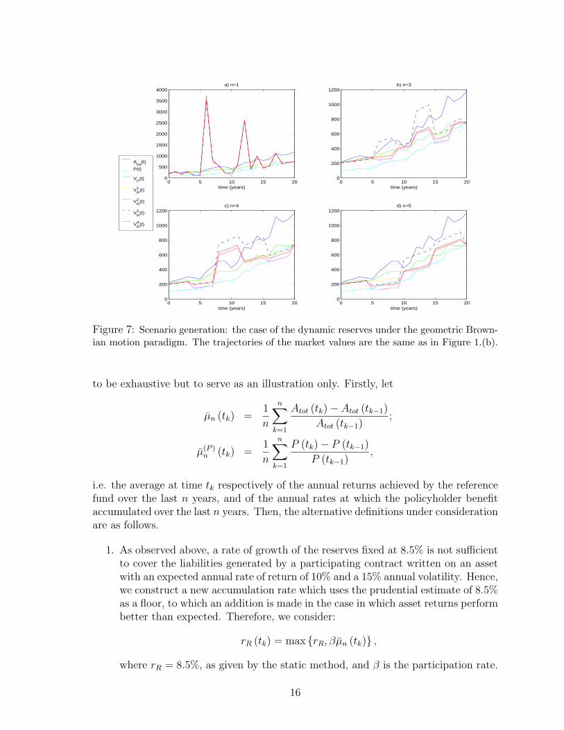
Figure 7: Scenario generation: the case of the dynamic reserves under the geometric Brown-ian motion paradigm. The trajectories of the market values are the same as in Figure 1.(b).
to be exhaustive but to serve as an illustration only. Firstly, let
µn (tk) =1
n
n∑k=1
Atot (tk) − Atot (tk−1)
Atot (tk−1);
µ(P )n (tk) =
1
n
n∑k=1
P (tk) − P (tk−1)
P (tk−1),
i.e. the average at time tk respectively of the annual returns achieved by the referencefund over the last n years, and of the annual rates at which the policyholder benefitaccumulated over the last n years. Then, the alternative definitions under considerationare as follows.
1. As observed above, a rate of growth of the reserves fixed at 8.5% is not sufficientto cover the liabilities generated by a participating contract written on an assetwith an expected annual rate of return of 10% and a 15% annual volatility. Hence,we construct a new accumulation rate which uses the prudential estimate of 8.5%as a floor, to which an addition is made in the case in which asset returns performbetter than expected. Therefore, we consider:
rR (tk) = max rR, βµn (tk) ,
where rR = 8.5%, as given by the static method, and β is the participation rate.
16

2. An alternative to the previous methods could be the replication of the benefit’saccumulation rate, so that:
rR (tk) = max rG, βµn (tk) ,
where rG = 4% is the minimum guarantee and β is the participation rate.
3. Since the principal goal for the establishment of reserves is to enable the companyto build over time sufficient resources to pay the benefits to the policyholder whendue, an alternative approach would be to make the accumulation rate rR (tk)dependent on the evolution of the benefit itself, rather than on the referencefund. In this case, we consider:
rR (tk) = maxrG, µ(P )
n (tk)
,
4. Finally, we propose an accumulation rate based on the extent to which the assetsperform above or below expectations. Let
sn (tk) = µn (tk) − µ
be the spread at time tk between the average of the last n years’ returns on theasset and its expected rate of return. Then we consider:
rR (tk) = rR + αsn (tk) ,
α =
β if sn (tk) > 0b < β if sn (tk) < 0,
where β is the participation rate. Hence, we allow for a smoothing method thatweights differently upwards or downwards movements of the reference fund. Thisasymmetric way of considering positive and negative movements in the assetreturns enables us to have at maturity the exact amount of resources to paythe full benefit to the policyholder, without overcharging the company duringunfavourable periods. In the simulations, we assume b = 40% against a partici-pation rate β = 80%.
Similarly to the analysis carried out for the static reserves, we plot in Figures 4-5the probabilities that the reserves calculated on the basis of the proposed methodsare below VP (t). We observe that P (VR (t) < VP (t)) drops very quickly, especiallyif the readjustment of the accumulation rate occurs every year. The “step-shape” ofthe curves, though, suggests that the trajectory followed by the reserves might notbe smooth. An example is shown in Figures 7-9, where we illustrate the evolutionover the lifetime of the policy of the proposed dynamic reserves corresponding to thespecific scenarios presented in Figure 1.(b), (d) and (f) respectively. As expected, forboth market paradigms considered in this paper, the evolution of the reserves is veryunstable and volatile, due to a number of high peaks occurring over the term of thecontract. The reason for this behaviour comes from the definition of the fictitious
17

0 5 10 15 200
500
1000
1500
2000
2500a) n=1
time (years)
S
tot(t)
P(t) V
P(t)
V1
R(t)
V2
R(t)
V3
R(t)
V4
R(t)
0 5 10 15 200
200
400
600
800
1000
1200b) n=3
time (years)
0 5 10 15 20100
200
300
400
500
600
700
800c) n=4
time (years)0 5 10 15 20
100
200
300
400
500
600
700
800d) n=5
time (years)
Figure 8: Scenario generation: the case of the dynamic reserves under the Levy processparadigm. The trajectories of the market values are the same as in Figure 1.(d).
0 5 10 15 200
0.5
1
1.5
2
2.5
3x 10
4 a) n=1
time (years)0 5 10 15 20
0
200
400
600
800
1000
1200b) n=3
time (years)
0 5 10 15 200
500
1000
1500c) n=4
time (years)0 5 10 15 20
0
200
400
600
800
1000
1200d) n=5
time (years)
S
tot(t)
P(t) V
P(t)
V1
R(t)
V2
R(t)
V3
R(t)
V4
R(t)
Figure 9: Scenario generation: the case of the dynamic reserves under the Levy processparadigm. The trajectories of the market values are the same as in Figure 1.(f).
18
1 2 3 4 5 6 7 8 9 10 11 12 13 14 15 16 17 18 19 20−0.2
0
0.2
0.4
0.6
Average of the last n years asset returns
time (years)
n=1n=3n=4n=5
1 2 3 4 5 6 7 8 9 10 11 12 13 14 15 16 17 18 19 200
0.1
0.2
0.3
0.4
Average of the last n years benefit returns
time (years)
1 2 3 4 5 6 7 8 9 10 11 12 13 14 15 16 17 18 19 20−0.4
−0.2
0
0.2
0.4
Levy process model: scenario 1
time (years)1 2 3 4 5 6 7 8 9 10 11 12 13 14 15 16 17 18 19 20
0
0.1
0.2
0.3
0.4
time (years)
1 2 3 4 5 6 7 8 9 10 11 12 13 14 15 16 17 18 19 20−0.4
−0.2
0
0.2
0.4
0.6Levy process model: scenario 2
time (years)1 2 3 4 5 6 7 8 9 10 11 12 13 14 15 16 17 18 19 20
0
0.1
0.2
0.3
0.4
0.5
time (years)
Brownian motion model
a) b)
c) d)
d) e)
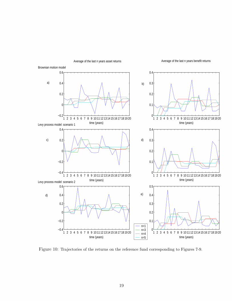
Figure 10: Trajectories of the returns on the reference fund corresponding to Figures 7-9.
19

account PR(T ), which represents the projection to maturity of the expected liability.This projection, in fact, is calculated using the information available at the reset dates,tk, about the past performance of the asset returns. Hence, the value of the optionsstill to be exercised is calculated on the basis of the past n years’ returns (illustratedin Figure 10) and the realized volatility over the same period, but, at the same time,ignoring the possible impact of the future market dynamic. This is particularly evidentwhen the readjustment of the accumulation rate, rR(t), occurs every year, i.e. for n = 1.In particular, we observe the size of the reserves in Figure 9, panel a, corresponding toyear 5. This is the effect of an increase in the equity fund of 57% between year 4 andyear 5 (see also panel d in Figure 10). As n increases, the smoothing effect becomesstronger and the peaks reduce in terms of both frequency and magnitude. The factthat the annual amount of the dynamic reserves is often greater than the fair value ofthe liability, means that, when compared to VP (t), the proposed reserving schemes arein a sense more expensive for the company to implement.
Retrospective method Finally, we consider the retrospective reserve, which iscalculated as the current amount of the policy reserve, i.e. the current amount of theaccumulated benefits, P (t), at time t.
The evolution of the retrospective reserve corresponding to the scenarios considered,is shown as well in Figures 7-9. We observe that P (t) is always below the estimatedvalue of the liabilities calculated using both the fair value approach and the dynamicreserving schemes discussed above, and the market value of the assets. This is asexpected since, by construction, the retrospective reserve does not account for the fullcost of the time value of the options and guarantees included in the contract design(see equation 5).
5 Solvency
The scenarios presented in section 4, and illustrated in Figures 7-9, show an additionalfeature deserving a more detailed analysis. The specific trajectories considered, in fact,suggest the possibility that the proposed dynamic reserves could be at a higher levelthan the total of the assets available to the company. Based on these scenarios, it isreasonable to expect periods in which the level of the reserves is above the total valueof the available assets, followed by periods in which the reserves drop below it. In termsof portfolio management, this implies that the insurer needs to adopt a very aggressiveinvestment strategy in order to balance the high level of the reserves, followed by largedisinvestments when these move below the assets level. Hence, compared to the fairvalue approach, estimating the value of the liabilities using a deterministic reservingscheme, such as the ones proposed above, could prove more expensive in terms of thecost of capital, with consequences for the solvency profile of the insurance company.
As mentioned in section 1, a new solvency regime, named “Solvency II”, is currentlydiscussed by the European Union with the aim of creating incentives to develop internalmodels for measuring the risk situation within insurance companies. The aim of this
20

section is to analyze, in the light of the guidelines arising from the Solvency II project,the capital requirements for an insurance company issuing a participating contract withminimum guarantee such as the one described in the previous sections. We considerhere only the valuation paradigm based on the Levy process model, with the premiumfor the default option invested in the same equity portfolio backing the policy (similarconclusions can be obtained for the geometric Brownian motion model as well; resultsare available from the authors).
Solvency II follows a three-pillar approach used in Basel II, so that Pillar 1 com-prises quantitative minimum requirements for equity capital provision; Pillar 2 dealswith supervisory review methods and the development of standards for sound internalrisk management; finally, Pillar 3 defines the requirements for disclosure obligationsand market transparency in order to ensure a high degree of market discipline. Morespecifically, one of the focus areas of Solvency II is to develop a formula for the calcu-lation of the target capital, i.e. the amount needed to ensure that the probability offailure of the insurance company within a given period is very low. This formula shouldbe based on the assessment of the future cashflows related to the policies in force andassets held. The assessment should take into account all relevant risks, and should becarried out by building on the IASB proposals and the latest IFRS. The time horizonproposed is one year, whilst longer term elements should be taken into account in Pillar2 (European Commission, 2004). Although a specific assumption for the most suitableconfidence level is still under discussion, the current practice in some countries such asthe Netherlands and the UK, suggests a 99.5% probability (i.e. the ruin probabilityof 1/200), which, broadly speaking, implies that the insurance company should be atleast of investment grade quality (“BBB”) in terms of rating.
Hence, as the target capital depends on the annual ruin probability, i.e. the proba-bility that the insurer will have not enough assets to cover the liabilities at the end ofthe observation period, we consider as a relevant index for our analysis, the differencebetween the market consistent value of the assets and the best estimate of the liabilitiesgenerated by the contract. As the best estimate of the liability we use its fair valueas calculated in section 2.1, and the estimates produced by the deterministic reservingmethods introduced in section 4. In the language of the Swiss Solvency Test (FOPI,2004), this index goes under the name of Risk Bearing Capital (RBC). For easy ofexposition, we express the RBC as percentage of the estimated liability, i.e.
RBC =Stot(t) − V (t)
V (t),
where V is the best estimate of the liability.We note that a reserving method which leads to an artificially low value of the
liabilities will have a P (RBC > 0) with desirable characteristics. We comment on thispossibility in a later paragraph.
In Figure 11, we represent the probability that at the end of each year the RBCis positive. These plots are accompanied by the analysis of the moments of the distri-bution of the RBC in each year, shown in Figures 12-14. Figures 12 and 13 relate tothe four dynamic reserving methods described in section 5, and Figure 14 relates to
21

0 5 10 15 200
0.2
0.4
0.6
0.8
1
a) V1R
(t)
time (years)
VR
(t)
(static method)
n=1 n=3 n=4 n=5 V
P(t)
0 5 10 15 200
0.2
0.4
0.6
0.8
1
b) V2R
(t)
time (years)
VR
(t)
(static method)
0 5 10 15 200
0.2
0.4
0.6
0.8
1
c) V3R
(t)
time (years)
VR
(t)
(static method)
0 5 10 15 200
0.2
0.4
0.6
0.8
1
d) V4R
(t)
time (years)
VR
(t)
(static method)
Figure 11: P(RBC > 0) for the benchmark set of parameters under the real probabilitymeasure. The distribution has been obtained using 100,000 scenarios. Each panel correspondsto one of the dynamic reserving method described in section 4.
the static reserving method. We observe that the fair value approach not only gener-ates the highest probability of being solvent (i.e. of having a positive RBC), but alsoguarantees a stable RBC over the lifetime of the contract and, consequently, reducedadditional injections of capital from the shareholders. This also implies that the fairvalue reporting system could prove helpful for the definition of an effective ALM policy.In contrast, the probabilities of being solvent originated by any of the four dynamic
reserving methods discussed in section 4, deteriorate very quickly with time (especiallyif the accumulation rate, rR(t), is readjusted every year). Moreover, the step-shape ofthe curves suggests that the capital requirements for the insurance company would bevery different one year from the other in terms of magnitude. This emerges also fromthe analysis of the moments of the distribution of the RBC. The irregular behaviour ofthe RBC’s variance, in particular, represents for the insurance company a significantproblem for the development and implementation of an effective strategy of internalrisk management.
Finally, in Figure 11 we note that the static reserving method leads to the high-est probability of solvency; however, this plot should be read together with Figure 5discussed in section 4. This latter Figure, in fact, shows that the reason for such aconsistently high RBC is due to the fact that the static reserve consistently underes-timates the fair value of the liability, to the extent that the reserves accumulated tillmaturity according to this method, fail to cover the actual amount of the benefits in92% of the cases. The very high variance of the RBC (in Figure 14) is instead due
22

0 5 10 15 20−1
−0.8
−0.6
−0.4
−0.2
0
0.2
0.4
0.6
0.8
Risk Bearing Capital − V1R
(t)
time (years)
mea
n
n=1 n=3 n=4 n=5 V
P(t)
0 5 10 15 20−1
−0.8
−0.6
−0.4
−0.2
0
0.2
0.4
0.6
0.8
Risk Bearing Capital − V2R
(t)
time (years)
mea
n
0 5 10 15 20−1
−0.8
−0.6
−0.4
−0.2
0
0.2
0.4
0.6
0.8
Risk Bearing Capital − V3R
(t)
time (years)
mea
n
0 5 10 15 20−1
−0.8
−0.6
−0.4
−0.2
0
0.2
0.4
0.6
0.8
Risk Bearing Capital − V4R
(t)
time (years)
mea
n
Figure 12: The mean of the risk bearing capital distribution resulting from the numericalexperiment described in Figure 11. The risk bearing capital is calculated as (Stot − V )/V ,where V is the best estimate of the liability provided by the four dynamic reserving schemesdescribed in section 4 and by the fair value VP (t).
0 5 10 15 200
0.05
0.1
0.15
0.2
0.25
0.3
0.35
0.4
Risk Bearing Capital − V1R
(t)
time (years)
varia
nce
n=1 n=3 n=4 n=5 V
P(t)
0 5 10 15 200
0.1
0.2
0.3
0.4
0.5
0.6
0.7
0.8
0.9
Risk Bearing Capital − V2R
(t)
time (years)
mea
n
0 5 10 15 200
0.1
0.2
0.3
0.4
0.5
0.6
0.7
0.8
0.9
Risk Bearing Capital − V3R
(t)
time (years)
varia
nce
0 5 10 15 200
5
10
15
20
25
Risk Bearing Capital − V4R
(t)
time (years)
varia
nce
Figure 13: The variance of the risk bearing capital distribution resulting from the numericalexperiment described in Figure 11. We note the magnitude of this moment of the distributionfor the reserving scheme 4.
23

0 5 10 15 200
0.5
1
1.5
2
2.5
Risk Bearing Capital − VR
(t)(static method)
time (years)
mean
0 5 10 15 200
1
2
3
4
5
6
time (years)
varia
nce
Figure 14: Mean and variance of the risk bearing capital distribution when the best estimateof the liability is given by the static reserve.
to the fact that the static reserves are completely uncorrelated with the movements ofthe assets (and hence the market volatility).
6 Concluding remarks
In this paper, we describe a fair valuation approach to setting the premium and reservesfor a simple, participating insurance policy, which includes in its design a minimumguaranteed rate and a participation rate (analogous to a reversionary bonus) and whichalso allows for the insurance company’s default option.
We demonstrate how an allowance for the default option in the premium (via asolvency loading) leads to a dramatic reduction in the probability of default for thecontract at maturity, for reasonable parameter values. This is also relevant in termsof risk management of the contract under consideration: the probability of default forthe case without a solvency loading, in fact, is too high for any hedging strategy to beable to be successfully effective.
An analysis of the model error and parameter error for the contract indicate thesensitivity of the results to the underlying assumptions and point to the need for aMarket Value Margin. In order to represent model error, we use the idea that theinsurance company assumes that its invested assets are accumulating according to ageometric Brownian motion process whereas in fact they are driven by a geometricLevy process.
An important conclusion of the analysis is that attempts to use deterministic re-serving methods for such a typical contract (defined along traditional lines) lead toundesirable results when compared with the fair valuation approach. These conclu-
24

sions are demonstrated in section 4 by our considering the probability that, at the endof each year, the value of the reserves is below the fair value of the liability – a prob-ability that we find to be unacceptably high. These conclusions are also supported bythe analysis in section 5 which considers the moments of the RBC distribution and theprobability that the RBC is positive at the end of each year, thereby demonstratingsolvency.
References
[1] Bacinello, A. R. (2001). Fair pricing of life insurance participating contracts witha minimum interest rate guaranteed. Astin Bulletin, 31, 275-97.
[2] Bakshi, G. S., Cao, C. and Chen, Z. (1997). Empirical performance of alternativeoption pricing models, Journal of Finance, 52, 2003-49.
[3] Ballotta, L. (2005). A Levy process-based framework for the fair valuation ofparticipating life insurance contracts, to appear in Insurance: Mathematics andEconomics.
[4] Ballotta, L., Haberman, S. and Wang, N. (2005). Guarantees in with-profit andunitised with profit life insurance contracts: fair valuation problem in presence ofthe default option, to appear in Journal of Risk and Insurance.
[5] Black, F. and M. Scholes (1973). The pricing of options on corporate liabilities,Journal of Political Economy, 81, 637-59
[6] Brennan, M. J. and E. S. Schwartz (1976). The pricing of equity-linked life insur-ance policies with an asset value guarantee, Journal of Financial Economics, 3,195-213.
[7] Carr, P., Geman. H., Madan D. B. and Yor M. (2002). The fine structure of assetreturns: an empirical investigation, Journal of Business, 75, 305-32.
[8] Daykin, C. D., Pentikainen, T. and Pesonen, E. (1994). Practical risk theory foractuaries. 1st edition, Chapman & Hall, London.
[9] Dickinson, G. and Liedtke, P. M. (2004). Impact of a fair value financial report-ing system on insurance companies: a survey. The Geneva Papers on Risk andInsurance, 29, 3, 540-81.
[10] European Commission (2004). Solvency II-Organization of work, discussion onPillar I work areas and suggestions of further work on Pillar II for CEIOPS. Noteto the IC Solvency Committee (February 2004).
[11] FASB (2004). Project update: fair value measurements.
[12] FitchRatings (2004). Mind the GAAP: Fitch’s view on Insurance IFRS.
25

[13] FOPI (2004). White Paper of the Swiss Solvency Test.
[14] FSA (2004). PS04/16. Integrated Prudential Sourcebook for Insurers.
[15] IASB (2004). International Financial Reporting Standard 4 - Insurance Contracts.
[16] Jørgensen, P. L. (2004). On accounting standards and fair valuation of life insur-ance and pension liabilities, Scandinavian Actuarial Journal, 5, 372-94.
[17] Miltersen, K., R. and S. A. Persson (2003). Guaranteed investment contracts:distributed and undistributed excess return, Scandinavian Actuarial Journal, 4,257-79.
26

1
FACULTY OF ACTUARIAL SCIENCE AND STATISTICS
Actuarial Research Papers since 2001
135. Renshaw A. E. and Haberman S. On the Forecasting of Mortality Reduction Factors. February 2001.
ISBN 1 901615 56 1 136. Haberman S., Butt Z. & Rickayzen B. D. Multiple State Models, Simulation and Insurer
Insolvency. February 2001. 27 pages. ISBN 1 901615 57 X
137. Khorasanee M.Z. A Cash-Flow Approach to Pension Funding. September 2001. 34 pages.
ISBN 1 901615 58 8
138. England P.D. Addendum to “Analytic and Bootstrap Estimates of Prediction Errors in Claims Reserving”. November 2001. 17 pages.
ISBN 1 901615 59 6
139. Verrall R.J. A Bayesian Generalised Linear Model for the Bornhuetter-Ferguson Method of Claims Reserving. November 2001. 10 pages.
ISBN 1 901615 62 6 140. Renshaw A.E. and Haberman. S. Lee-Carter Mortality Forecasting, a Parallel GLM Approach,
England and Wales Mortality Projections. January 2002. 38 pages. ISBN 1 901615 63 4
141. Ballotta L. and Haberman S. Valuation of Guaranteed Annuity Conversion Options. January
2002. 25 pages. ISBN 1 901615 64 2
142. Butt Z. and Haberman S. Application of Frailty-Based Mortality Models to Insurance Data. April
2002. 65 pages. ISBN 1 901615 65 0
143. Gerrard R.J. and Glass C.A. Optimal Premium Pricing in Motor Insurance: A Discrete
Approximation. (Will be available 2003). 144. Mayhew, L. The Neighbourhood Health Economy. A systematic approach to the examination of
health and social risks at neighbourhood level. December 2002. 43 pages.
ISBN 1 901615 66 9 145. Ballotta L. and Haberman S. The Fair Valuation Problem of Guaranteed Annuity Options: The
Stochastic Mortality Environment Case. January 2003. 25 pages.
ISBN 1 901615 67 7
146. Haberman S., Ballotta L. and Wang N. Modelling and Valuation of Guarantees in With-Profit and Unitised With-Profit Life Insurance Contracts. February 2003. 26 pages.
ISBN 1 901615 68 5
147. Ignatov Z.G., Kaishev V.K and Krachunov R.S. Optimal Retention Levels, Given the Joint Survival of Cedent and Reinsurer. March 2003. 36 pages.
ISBN 1 901615 69 3 148. Owadally M.I. Efficient Asset Valuation Methods for Pension Plans. March 2003. 20 pages.
ISBN 1 901615 70 7

2
149. Owadally M.I. Pension Funding and the Actuarial Assumption Concerning Investment Returns. March 2003. 32 pages.
ISBN 1 901615 71 5
150. Dimitrova D, Ignatov Z. and Kaishev V. Finite time Ruin Probabilities for Continuous Claims Severities. Will be available in August 2004.
151. Iyer S. Application of Stochastic Methods in the Valuation of Social Security Pension Schemes.
August 2004. 40 pages. ISBN 1 901615 72 3
152. Ballotta L., Haberman S. and Wang N. Guarantees in with-profit and Unitized with profit Life
Insurance Contracts; Fair Valuation Problem in Presence of the Default Option1. October 2003. 28 pages.
ISBN 1-901615-73-1
153. Renshaw A. and Haberman. S. Lee-Carter Mortality Forecasting Incorporating Bivariate Time Series. December 2003. 33 pages.
ISBN 1-901615-75-8
154. Cowell R.G., Khuen Y.Y. and Verrall R.J. Modelling Operational Risk with Bayesian Networks. March 2004. 37 pages.
ISBN 1-901615-76-6 155. Gerrard R.G., Haberman S., Hojgaard B. and Vigna E. The Income Drawdown Option:
Quadratic Loss. March 2004. 31 pages. ISBN 1-901615-77-4
156. Karlsson, M., Mayhew L., Plumb R, and Rickayzen B.D. An International Comparison of Long-
Term Care Arrangements. An Investigation into the Equity, Efficiency and sustainability of the Long-Term Care Systems in Germany, Japan, Sweden, the United Kingdom and the United States. April 2004. 131 pages.
ISBN 1 901615 78 2 157. Ballotta Laura. Alternative Framework for the Fair Valuation of Participating Life Insurance
Contracts. June 2004. 33 pages. ISBN 1-901615-79-0
158. Wang Nan. An Asset Allocation Strategy for a Risk Reserve considering both Risk and Profit.
July 2004. 13 pages. ISBN 1 901615-80-4
159. Spreeuw Jaap. Upper and Lower Bounds of Present Value Distributions of Life Insurance
Contracts with Disability Related Benefits. December 2004. 35 pages. ISBN 1 901615-83-9
160. Renshaw A.E. and Haberman S. Mortality Reduction Factors Incorporating Cohort Effects.
January 2005. 33 pages. ISBN 1 90161584 7
161. Gerrard R.J. Haberman A and Vigna E. The Management of De-Cumulation Risks in a Defined
Contribution Environment. February 2005. 35 pages. ISBN 1 901615 85 5.
162. Ballotta L, Esposito G. and Haberman S. The IASB Insurance Project for Life Insurance
Contracts: Impart on Reserving Methods and Solvency Requirements. May 2005. 26 pages. ISBN 901615 86 3.

3
Statistical Research Papers 1. Sebastiani P. Some Results on the Derivatives of Matrix Functions. December 1995. 17 Pages.
ISBN 1 874 770 83 2 2. Dawid A.P. and Sebastiani P. Coherent Criteria for Optimal Experimental Design. March 1996. 35 Pages.
ISBN 1 874 770 86 7 3. Sebastiani P. and Wynn H.P. Maximum Entropy Sampling and Optimal Bayesian Experimental
Design. March 1996. 22 Pages. ISBN 1 874 770 87 5
4. Sebastiani P. and Settimi R. A Note on D-optimal Designs for a Logistic Regression Model. May
1996. 12 Pages. ISBN 1 874 770 92 1
5. Sebastiani P. and Settimi R. First-order Optimal Designs for Non Linear Models. August 1996. 28
Pages. ISBN 1 874 770 95 6
6. Newby M. A Business Process Approach to Maintenance: Measurement, Decision and Control.
September 1996. 12 Pages. ISBN 1 874 770 96 4
7. Newby M. Moments and Generating Functions for the Absorption Distribution and its Negative
Binomial Analogue. September 1996. 16 Pages. ISBN 1 874 770 97 2
8. Cowell R.G. Mixture Reduction via Predictive Scores. November 1996. 17 Pages.
ISBN 1 874 770 98 0 9. Sebastiani P. and Ramoni M. Robust Parameter Learning in Bayesian Networks with Missing
Data. March 1997. 9 Pages. ISBN 1 901615 00 6
10. Newby M.J. and Coolen F.P.A. Guidelines for Corrective Replacement Based on Low Stochastic
Structure Assumptions. March 1997. 9 Pages. ISBN 1 901615 01 4.
11. Newby M.J. Approximations for the Absorption Distribution and its Negative Binomial Analogue.
March 1997. 6 Pages. ISBN 1 901615 02 2
12. Ramoni M. and Sebastiani P. The Use of Exogenous Knowledge to Learn Bayesian Networks from
Incomplete Databases. June 1997. 11 Pages. ISBN 1 901615 10 3
13. Ramoni M. and Sebastiani P. Learning Bayesian Networks from Incomplete Databases. June 1997. 14 Pages.
ISBN 1 901615 11 1 14. Sebastiani P. and Wynn H.P. Risk Based Optimal Designs. June 1997. 10 Pages.
ISBN 1 901615 13 8 15. Cowell R. Sampling without Replacement in Junction Trees. June 1997. 10 Pages.
ISBN 1 901615 14 6 16. Dagg R.A. and Newby M.J. Optimal Overhaul Intervals with Imperfect Inspection and Repair. July
1997. 11 Pages. ISBN 1 901615 15 4
17. Sebastiani P. and Wynn H.P. Bayesian Experimental Design and Shannon Information. October 1997. 11 Pages. ISBN 1 901615 17 0
18. Wolstenholme L.C. A Characterisation of Phase Type Distributions. November 1997. 11 Pages. ISBN 1 901615 18 9

4
19. Wolstenholme L.C. A Comparison of Models for Probability of Detection (POD) Curves. December
1997. 23 Pages. ISBN 1 901615 21 9 20. Cowell R.G. Parameter Learning from Incomplete Data Using Maximum Entropy I: Principles.
February 1999. 19 Pages. ISBN 1 901615 37 5 21. Cowell R.G. Parameter Learning from Incomplete Data Using Maximum Entropy II: Application to
Bayesian Networks. November 1999. 12 Pages ISBN 1 901615 40 5 22. Cowell R.G. FINEX : Forensic Identification by Network Expert Systems. March 2001. 10 pages.
ISBN 1 901615 60X
23. Cowell R.G. When Learning Bayesian Networks from Data, using Conditional Independence Tests
is Equivalant to a Scoring Metric. March 2001. 11 pages. ISBN 1 901615 61 8
24. Kaishev, V.K., Dimitrova, D.S., Haberman S., and Verrall R.J. Autumatic, Computer Aided
Geometric Design of Free-Knot, Regression Splines. August 2004. 37 pages. ISBN 1-901615-81-2
25. Cowell R.G., Lauritzen S.L., and Mortera, J. Identification and Separation of DNA Mixtures Using
Peak Area Information. December 2004. 39 pages. ISBN 1-901615-82-0

Faculty of Actuarial Science and Statistics
Actuarial Research Club
The support of the corporate members
CGNU Assurance Computer Sciences Corporation
English Matthews Brockman Government Actuary’s Department
Watson Wyatt Partners
is gratefully acknowledged.
ISBN 1-901615-86-3