1

The Impact of Agricultural Productivity on Welfare Growth of Farm

Households in Nigeria: A Panel Data Analysis

Mulubrhan Amarea*, Jennifer Denno Cisséb, Nathaniel D. Jensenb and Bekele

Shiferawa

a*Corresponding author: Research Fellow, Partnership for Economic Policy (PEP),

PO.Box:30772-01100, Nairobi, Kenya. E-mail: Mulubrhan.Amare@pep-net.org

b Cornell University, Charles H. Dyson School of Applied Economics and Management, Ithaca,

New York 14853, USA

Abstract

Empirical studies across many developing countries document that improving agricultural

productivity is the main pathway out of poverty. In this paper, we begin by investigating the factors

that hinder or accelerate agricultural productivity. Additionally, we seek to understand whether

agricultural productivity, measured using land productivity, improves household consumption

growth using nationally representative Living Standards Measurement Study - Integrated Surveys

on Agriculture (LSMS-ISA) panel datasets from Nigeria, merged with detailed novel climate and

bio-physical information. The results show that agricultural productivity is positively associated

with labor and farm inputs. Consistent with the inverse land size-productivity relationship so often

observed in the literature, land productivity decreases with increasing farm size. We also find that

climate risk and bio-physical variables play a significant role in explaining agricultural

productivity. Moreover, agricultural productivity has a significant and positive impact on

household consumption growth. The results also indicate that while agricultural productivity has

a positive impact on welfare growth for non-poor households, it has a negative impact for poor

households.

2

1. Introduction

Agriculture constitutes only about one-fifth of Africa’s GDP and about half of the total value of

its exports, yet more than two-thirds of the population lives in rural areas and more than 85% of

people in these regions depended on agriculture for their livelihoods (World Bank Development

Indicators, 2014). Improving the productivity, profitability, and sustainability of smallholder

farming is therefore considered the main pathway out of poverty. Agricultural research and

development interventions focused on agricultural intensification and modernizing market

channels for agricultural products can lead to agricultural productivity growth and thereby both

reduce poverty and meet growing demands for food (Ravallion and Datt, 1998; Loayza and

Raddatz, 2010; Ravallion and Datt, 1999, Mellor, 2001; Thirtle et al., 2003).

The literature suggests that there are multiple pathways through which increases in

agricultural productivity can reduce poverty, including real income changes, employment

generation, rural non-farm multiplier effects, and food price effects (Ravallion and Datt, 1999,

Gollin et al., 2002; Irz and Tiffin, 2006). Its impact on poverty is both direct, flowing immediately

from growth in agriculture by raising real incomes of poor farm (and non-farm) households, and

indirect by increasing agricultural outputs which induces job creation in upstream and downstream

non-farm sectors as a response to higher domestic demand (Valde´s and Foster, 2007; Gollin et

al., 2014). Potentially lower food prices can increase the purchasing power of poor consumers

(Olsson and Hibbs, 2005; de Janvry and Sadoulet, 2010). The poverty impact of agricultural

productivity can be sizeable mainly because the majority of poor people in sub-Saharan Africa

countries directly depend on agriculture for their livelihoods (Foster and Rosenzweig, 2005).

However, agriculture is not a panacea for poverty reduction (Hasan and Quibria, 2004).

Agriculture is often associated with economic and natural risks such as price fluctuations, drought,

pests and diseases. The poor and small-scale farmers are particularly vulnerable to these risks. A

country which relies on agricultural exports can be adversely affected by global economic shocks

(Winters et al., 2004; Easterly and Kraay, 2000). A sudden decrease in the prices of agricultural

outputs can quickly push small net sellers into losses and poverty. Moreover, poor smallholders

face a number of constraints that limit their productivity. Lack of information about production

methods and market opportunities, particularly for new crops and varieties prohibit households

from intensifying agriculture and producing high-value commodities whose market demand is

growing rapidly. Poor access to credit and/or insurance can also limit uptake of new technologies.

Smallholder producers are now also facing the growing challenges of recent technological changes

3

and the stringent quality standards for many food products, both of which are associated with the

globalization of commodity chains. In addition, high initial inequality in the distribution of assets

and especially of land can also be a plausible candidate explanation of why some agricultural

productivity change might be less effective in up lifting poor families from poverty (de Janvry and

Sadoulet, 2010).

Therefore, the extent to which poor people would gain from agricultural productivity

depends on the specific circumstances of initial land distribution, market, infrastructure,

institutions and demographic set ups. Our analysis is organized around four questions. First, what

are the main production determinants factors associated with of household agricultural

productivity? Second, how does agricultural productivity impact household welfare growth?

Third, does the relative position of poor people (e.g. the bottom 25%) improve or worsen with

productivity change? Fourth, how do different categories of smallholder farmers benefit from

agricultural productivity?

The paper contributes to the literature in several respects. First, whereas earlier research

has examined the relationship between farm technology and agricultural productivity, and farm

technology and household welfare, there is limited evidence on how agricultural productivity

change affects household welfare growth. Second, the paper uses panel data from a nationally

representative household level survey with rich socio-economic information, merged with detailed

novel climate and bio-physical information. The combination of these datasets allows us to assess

the role of weather in determining households’ agricultural productivity and its impact on

household welfare growth. Third, a key issue that has not been adequately addressed in the

agricultural productivity and household welfare linkages literature is unobserved heterogeneity

which could cause endogeneity. In this paper, we investigate the impact of agricultural productivity

on household welfare growth taking explicitly into account the potential endogeneity of

agricultural productivity using exogenous climate and bio-physical variables as instrument

variables. Fourth, the paper provides evidence on impact of agricultural productivity on different

categories of smallholder farmers, such as by welfare status and initial land holdings, with

important policy implications in designing specific policies for specific categories of households.

We find that agricultural productivity is positively associated with labor and farm inputs.

Consistent with the inverse land size-productivity relationship so often observed in the literature,

land productivity decreases with increasing farm size. We also find that climate risk and bio-

physical variables play a significant role in explaining agricultural productivity. Moreover,

4

agricultural productivity has a significant and positive impact on household consumption growth.

The results also indicate that while agricultural productivity has a positive impact on welfare

growth for non-poor households, it has a negative impact for poor households.

The paper is organized as follows: Section 2 presents the background on agricultural

production and productivity in Nigeria. Section 3 elaborates data and descriptive statistics. Section

4 presents the empirical model and identification strategy. The empirical results are presented in

Section 5 before we conclude in the final section, highlighting the main findings and policy

implications.

2. Background: Agricultural Production and Productivity in Nigeria

Nigeria is the largest country in Africa in terms of population (177 million) and among the largest

in terms of land area (910,770 km2). Nigeria has the 27th biggest economy in the world, with a

gross domestic product (GDP) of US$523 billion; its per capita GDP was US$3,010 in 2013

(World Bank 2014). The agricultural sector employs 60 % of Nigeria’s working population and

accounts for over 40 % of its GDP, although a higher level of poverty is observed among

households whose primary source of income is agriculture (World Bank, 2014). As for subsectors,

crop production captures the largest share — estimated at 88 % of the total GDP from agriculture

(Mogues et al., 2014). The agricultural sector in Nigeria grew by about 5.9 % annually from 2002

to 2012, but it is argued that the growth in the agricultural sector is mainly attributed to population

growth and the farming of larger expanses of land, most likely by commercial farmers (Oseni et

al., 2014). Nigerian agriculture is primarily rain-fed, which is characterized by low productivity,

low technology, and high labor intensity.

This low agricultural productivity has been attributed to the low use of fertilizer, the loss

of soil fertility, and traditional, low technology, rain-fed farming systems. The literature has

documented that Nigerian farmers across all regions are below their production frontiers,

indicating there is room to increase agricultural productivity above existing levels, even without a

change in their current levels of input use (Liverpool-Tasie et al., 2011; Oseni and Winters, 2009).

Low input use and farm technology, such as improved seed and fertilizer, are among the many

reasons for low agricultural productivity in Nigeria. More than 80% of the households in Nigeria

relate their poverty status to problems in agriculture, of which lack of agricultural inputs and not

being able to afford inputs (such as fertilizers and seeds) accounts for 44 % (Oseni and Winters,

2009). Moreover, the Federal Ministry of Agriculture and Rural Development estimated fertilizer

5

application at 10-15 kg/ha in 2009, far lower than the 200 kg/ha recommended by the United

Nations Food and Agriculture Organization (FAO). The huge gap in fertilizer use compared to

recommended fertilizer levels is often given as one of the main reasons for low agricultural

productivity in Nigeria. It has long been argued that limited access of framer to extension service,

an outdated land tenure system, climatic factors, imperfect credit and capital market, spatial

inequality distribution of fertilizer, the high prices of other non-fertilizer inputs and an inadequate

fertilizer supply are among other constraints to improve fertilizer use in Nigeria (Philip et al., 2009;

Oseni et al., 2014).

Nigeria, along with some other Sub-Saharan African countries (e.g., Malawi, Kenya,

Tanzania, Zambia, and Zimbabwe), implemented fertilizer subsidy programs in the 1970s where

both Federal and State governments directly procured fertilizer from importers and distributed

subsidized fertilizer to farmers. The fertilizer subsidy has been central to the policy tool of Nigeria

to encourage growth in the agriculture sector and may be justified on many grounds, including

market failures (Mogues et al., 2012). Although fertilizer subsidies assisted Nigerian farmers to

expand fertilizer use to some extent, findings show that the heavy emphasis on price subsidization

to the detriment of other approaches — including complementary actions to improve farmers’

fertilizer-use techniques, seeking lower transactions costs, or reducing agricultural risk — has

hampered market development in Nigeria (Smith et al. 1994; Yanggen et al. 1998). To address the

issues and improve the usage of fertilizer as a means to achieving the region’s green revolution

objectives, the Federal Government of Nigeria (FGN) decided to disengage from direct

procurement of fertilizer in favor of promoting private sector participation and piloted a fertilizer

voucher system in selected Nigerian states as an alternative way of administering the fertilizer

subsidy. However, the impact of the experimental voucher program on improving fertilizer and

other input use, as well as on agricultural productivity are still inclusive.

3. Data and Descriptive Statistics

3.1. Data

The longitudinal data for this paper comes from the Nigerian LSMS-ISA, representing the years

2010 and 2012. The LSMS-ISA datasets are publicly available and were collected in eight African

countries. These nationally representative datasets include detailed information on household

characteristics such as education, demographic characteristics, household shocks, assets,

agricultural production, non-farm income, other sources of income, allocation of family labor,

6

hiring of labor, access to services, and consumption expenditure. The agriculture module includes

information on agricultural and livestock production, farm technology, use of modern inputs, and

productivity of crops and livestock. The community-level module contains information on local

level infrastructure, basic public goods, precipitation and %age of agricultural land that could

potentially affect agricultural production and productivity.

In order to control for the effects of rainfall and temperature variations on farmers’ adoption

agricultural productivity, we merge the Nigeria LSMS-ISA with historical rainfall and temperature

data at the enumeration area (EA) level. Rainfall and temperature data come from the daily Africa

Rainfall Climatology Version 2 (ARC2) of the National Oceanic and Atmospheric

Administration’s Climate Prediction Center (NOAA-CPC) summed at decadal (10-day) values and

corrected for possible missing daily values. The ARC2 rainfall database contains raster data at a

spatial ground resolution of 1/10 of degree for African countries for the period 1983-2012. Our

temperature data are decadal surface temperature measurements for the period of 1990-2012.

Similar to previous studies (e.g., Arslan et al., 2016; Asfaw et al., 2016), we construct

climate variability using coefficient of variation1 (CoV) rainfall and average rain shortfall, both

computed for the 1983-2012 period. One of the major advantages of the CoV in our context is that,

for a given level of standard deviation, it changes as the mean changes, reporting a lower level of

variability if the mean increases but the variance remains constant. On the other hand, CoV is

scale-invariant. The average rainfall shortfall is the average of the annual total departures from the

long run average. We also construct variables for total rainfall and mean monthly temperature

(1990-2012). We expect the climate indicators are important determinants of agricultural

productivity. To control for bio-physical characteristics and assess the impact of bio-physical

variables on agricultural productivity, we construct a variable of soil nutrient availability and soil

pH extracted from Harmonized World Soil (HWS) database2 and ISRIC-World Information

1The coefficient of variation (CoV of rainfall) is measured as the standard deviation divided by the mean

of the annual rainfall totals for 30 years (1983–2012) of (average/15Km EA radius).

2The database has a spatial resolution of 1km (30 arc seconds). http://www.fao.org/soils-portal/soil-

survey/soil-maps-and-databases/harmonized-world-soil-database-v12/en/

7

Service3, respectively. Soil pH values are at a spatial resolution of 1000 meters for the period 1950-

2005.

3.2. Descriptive statistics

As the main objective of this paper is to examine the drivers of agricultural productivity and its

impact on household welfare growth, only households who have harvested some crops for both of

the two years in the dataset were retained. This procedure resulted in a balanced panel of 2,031

households over two rounds. We measure aggregate household expenditure from both food and

non-food expenditures, income, assets and the total value of crops adjusted using regional CPI to

2010 purchasing power parity for Nigeria.

Table 1 reports land productivity by land and consumption quintile. The results indicate

that land productivity decreases with land size. Households in the bottom two quantiles exhibit

systematically higher productivity as compared to households in the two upper quintiles. The

results are consistent with the empirical evidence for the existence of an inverse farm size

productivity relationship (e.g. Carletto et al., 2013; Barrett et al., 2010). Table 1 also shows that

households in the bottom consumption quintile have lower land productivity. Similarly, Table 2

breaks down land productivity by land quintile and consumption quintile simultaneously. The

observations are surprisingly well distributed, although we do see a concentration of households

will relatively high (top quintile) consumption but low land holdings. We also see that the least

endowed households from a land holdings perspective are the most productive. There is no

discernable pattern, however, with regards to consumption. While households in the lowest

consumption quintile are never the most productive, we do not see that households with the highest

consumption are consistently more productive.

Table 3 describes land productivity and aggregate consumption by regions. There are

variations in land productivity across the zones. The South-South zone has the highest land

productivity, whereas the South-West and North-East zones have the lowest land productivity. We

speculate this may be attributable in part to labor constraints in South-West, including the

availability of non-farm employment in urban areas. This is because many of the major industries

and cities in the country are located in the South-West due to the presence of crude oil and the

3The values are for the 0-5cm depth. The soil pH maps can be downloaded from the ISRIC website at:

http://www.isric.org/data/soil-property-maps-africa-1-km

8

availability of ports whereas in northern parts of Nigeria households are more likely to be engaged

in agriculture and have larger farm sizes, as well as higher crop expenses. The infrastructural,

institutional, and socio-cultural variations across the zones may also contribute to high regional

variations in agricultural productivity.

Similarly, there are variations in aggregate consumption per adult equivalent across the

zones (Table 3). Southern zones have the highest aggregate consumption per adult equivalent as

compared to the Northern zones. South-West has the highest aggregate consumption per adult

equivalent (138,000 Nigerian naira per adult equivalent per year), whereas North-West has the

lowest (84,000 per adult equivalent per year). Poverty levels vary across the country with the

highest proportion of poor people in the Northern part of Nigeria (e.g. in North-Central about 29

% of the population is poor) and the lowest in the southern part of Nigeria (in South-West only 9

% of the population is poor)

Table 4 reports aggregate consumption by consumption quintile and round. We find that

aggregate annual consumption declined significantly in 2012 in all consumption quintiles. The

results reveal the %age change (drop) in aggregate consumption increases with aggregate

consumption; the highest decline is for the top consumption quintile households (26%).

To confirm that the climate and soil nutrient variables are important variables in explaining

agricultural productivity, we regress land productivity on climate variables, soil nutrient indicators

and other explanatory variables. Table 5 reports the results of this regression. To control for

differences in topology, land fertility, and other agro-ecological factors, state fixed effects are

included. We expect a high coefficient of rainfall variation imposes a production risk, which

subsequently makes adoption of farm technology riskier and thus reduces agricultural productivity,

while rainfall is expected to increase productivity. Land productivity is significantly, negatively

associated with rainfall CoV, rainfall shortfall, temperature and soil-nutrients and significantly,

positively associated with total rainfall. The coefficients are as expected.

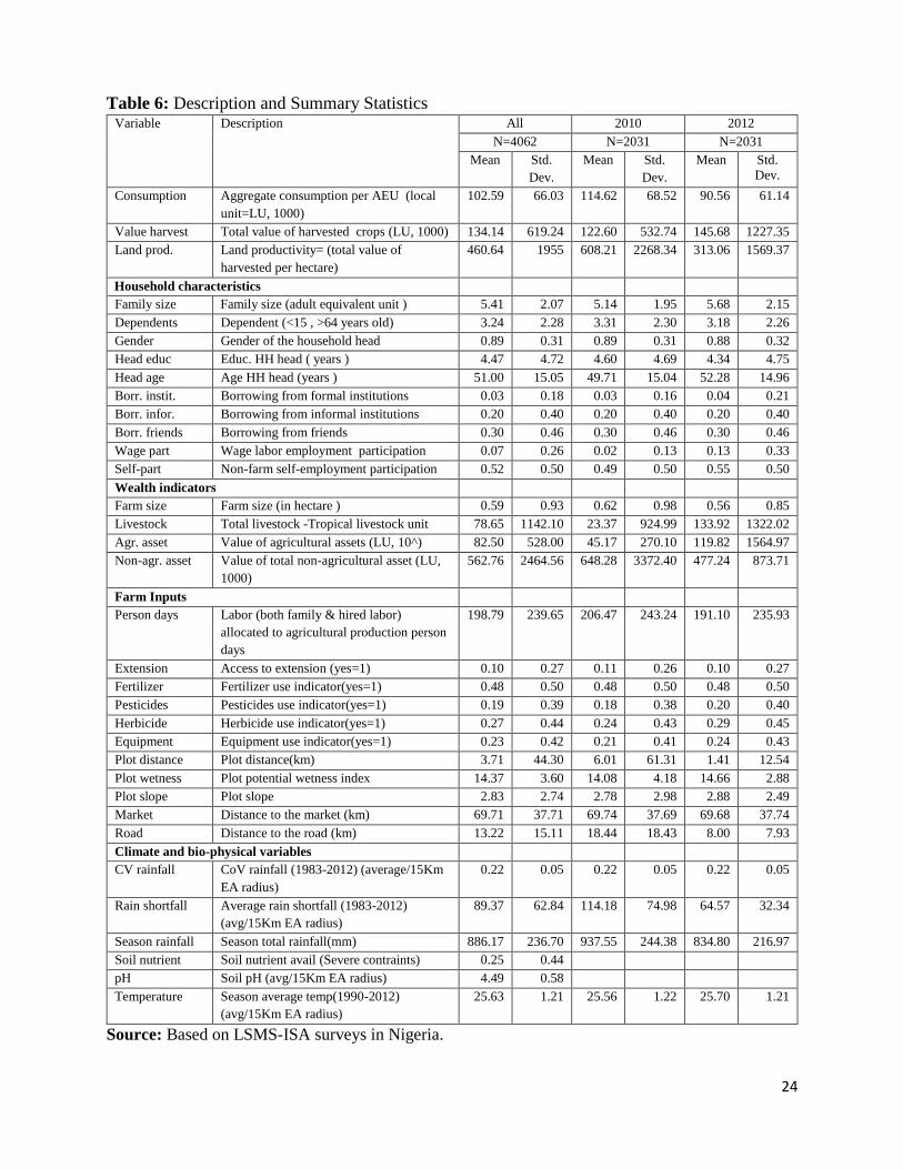
Summary statistics of the variables used in subsequent regression analyses are presented

in Table 6, including mean values for aggregate annual consumption per adult equivalent,

agricultural productivity, demographic characteristics (household size, education, age, and

gender), and wealth indicators including land and livestock, and both total and agricultural assets.

Table 6 also reports descriptive results of access to farm technology, infrastructure and financial

institutions, as well as climate and soil-nutrient variables. The average annual aggregate

consumption per AEU is about 103 (in thousands of Naira) and average land productivity is about

9

460 (thousand Naira) per hectare. Our key variables of interest are agricultural productivity

measured through land productivity (as described in the following section), annual aggregate

consumption per adult equivalent, and climate and soil-nutrient variables.

4. Empirical Approach

In this section we discuss the empirical approach to investigate two main objectives stated in the

introduction. First, we examine the drivers of household agricultural productivity. Second we

address the impact of agricultural productivity on household welfare growth in Nigeria. In

particular, we discuss how we control a key problem, endogeneity in agricultural productivity, in

estimating the impact of agricultural productivity on household welfare growth.

Given that factor markets are absent or imperfect in rural areas of developing countries, the

paper employs a non-separable (between production and consumption decisions) farm household

model (Singh et al., 1986; de Janvry et al., 1991) as the key conceptual framework. We assume

that households’ (denoted by 𝑖) objective is to maximize farm profit (𝜋), defined as:

𝜋𝑖 = ∑ 𝑝𝑦𝑌𝑖 − ∑ 𝑤𝑥 𝑋𝑖 (1)

where 𝑝 the vector of output prices and 𝑤 is is a vector of variable input prices. The production

function is given:

𝑌𝑖 = 𝑓(𝑋𝑖, 𝑘𝑖, 𝜔) (2)

where 𝑌 is the value of output per hectare, 𝑋 is a vector of quantities of variable inputs, 𝑘 is a

vector of quantities of quasi-fixed inputs, and 𝜔 is a vector of environmental variables (climate

variables, soil type, location, constraints, policy indicators etc.). Since labor and capital market

imperfections are common in developing countries, the shadow cost of labor and shadow cost of

capital are endogenous (Sadoulet & De Janvry, 1995). In other words, the shadow cost of labor

and capital are affected by household labor and asset endowments, as well as by village capital

and accessibility to infrastructure.

We measure agricultural productivity through analysis of the productivity of land.

Increasing land productivity is expected to play a significant role in improving household welfare

growth where population pressure on the land is high and the intensity of cultivation has increased

due to reduced fallow periods. Application of new technology (e.g. using improved seeds and

10

fertilizer) is important for increasing productivity of land as land scarcity increases. We measure

land productivity as the ratio of net-value of crop output per unit of land, i.e., net-income of

harvested produce per hectare. We use a Cobb-Douglas production function as follows:

ln (𝑌𝑖𝑡) = 𝛾𝑖𝑡 + ln(𝑋𝑖𝑡) β𝑥 + 𝐻𝑖𝑡𝛼ℎ + 𝐶𝑖𝑡𝛾𝑖 + 𝜈𝑖 + 𝜀𝑖𝑡 (3)

where 𝑋 is a vector of quantities of inputs such as: labor inputs, seeds, fertilizer, herbicide and

pesticides. We expect all the farm technology variables to contribute positively to the increase

productivity. 𝐻 is a vector household and community characteristics such education, the age,

gender of the household head and household size assets and community-characteristics. We expect

that households with more labor and educated household heads are more likely to have higher

agricultural productivity, because they are better able to employ the new technologies, either

because education helps them learn about how to use the technology and\or education is related to

other unobserved things that result in variation in production from technology. 𝐶 is a vector of

climate variables and soil type. 𝜈 is a household specific fixed effect, and 𝜀 is a mean zero,

identically and independently distributed random error and is assumed to be uncorrelated to all the

explanatory variables.

The problem in estimating the drivers of agricultural productivity on welfare is that

agricultural productivity is correlated with the household’s level of information about inputs, level

of human capital and physical assets and unobserved heterogeneities (unobserved variation in plot

characteristics, managerial skill or ability). This correlation between the unobserved individual

effect in the error term 𝜀𝑖𝑡 and agricultural productivity would cause a bias in ordinary least squares

(OLS) estimators (Wooldridge, 2010). While the fixed effects model addresses bias caused by time

variant and time invariant factors that are endogenous, it only addresses time-invariant

unobservable heterogeneities (dimensions of soil quality and geographic variables that might affect

agricultural) so that the estimates of the other variables are not biased by time-invariant variables.

Thus, we employ the Correlated Random Effects (CRE) model which enables us to address time

invariant unobserved household characteristics and still recover the coefficients on time invariant

variables (Mundlak 1978; Chamberlain, 1982). The estimation procedure in CRE involves adding

the mean of time-varying variables as an extra set of explanatory variables. The inclusion of these

mean variables controls for time-constant unobserved heterogeneity (Wooldridge, 2010).

11

We estimate the impact of agricultural productivity measured using land productivity on

household consumption growth using a function of the following form:

Δ𝐶𝑖𝑡 = γ1P𝑖𝑡−1 + γ2H𝑖𝑡−1 + γ3𝑊𝑖𝑡−1 + γ4𝐿𝑖𝑡−1 + γ5𝐶𝑖𝑡−1 + 𝜍 + 𝜆𝑝 + 𝜂𝑖 (4)

The dependent variable used in the regression analysis is the adjusted per capita consumption

growth(Δ𝐶𝑖𝑡). The effect of interest is captured by the coefficients on P𝑖𝑡−1, which is land

productivity (total net-value of harvest per hectare). H𝑖𝑡 represents a vector of levels of household

demographic characteristics and 𝑊𝑖𝑡 captures household wealth indicators. To explore the effect

of extension service and plot characteristics (𝐿𝑖𝑡) on consumption and asset, we include

information on the frequency of contact with extension agents, the plot slope and potential wetness

index.

We also include community characteristic assets (𝐶𝑖𝑡) agricultural potential and access to

market and road. Community variables are included in the equation because they represent the

availability of productive economic infrastructure due to infrastructure investments by service

providers which is closely associated with non-farm and other income-generating activities in the

local environment. Because similar intrinsic demographic characteristics can lead to different asset

distribution patterns, a household fixed effect 𝜍 is included to control for time-invariant unobserved

demographic characteristics. Furthermore, a state fixed effect (𝜆𝑝) is included to control for further

geographic diversity in land quality, weather conditions, and distance to markets, local leadership,

and for covariate shocks affecting all provinces uniformly in each year. 𝜂𝑖 is the error term for

which strict a exogeneity condition is assumed to hold; errors are independently and normally

distributed with zero mean and constant variance.

It is likely that agricultural productivity is correlated with household level of farm

technology information, level of human capital and physical assets and unobserved heterogeneities

(e.g., unobserved variation in plot characteristics, managerial skill or ability). This correlation

between the unobserved individual effect in the error term 𝜂𝑖 and agricultural productivity would

cause a bias in ordinary least squares (OLS) estimators (Hausman and Taylor 1981).

To address for this type of endogeneity, we use a set of instrumental variables that influence

welfare growth which is measured by changes to consumption only through their effect on the

household’s agricultural productivity. We construct the instruments by matching our panel

household data with the historical rainfall data and soil type. We use the coefficient of variation

12

and the average shortfall of rainfall computed over the period 1983-2012 at EA the level, which

are intended to capture the uncertainty about expected climatic conditions, and soil type of the EA.

Our justification for using these instruments is that the coefficient of variation of and average

shortfall of rainfall and soil-nutrients influence agricultural productivity without directly

influencing the welfare growth in the village.

A potential concern with regard to the validity of the instrument is that the use the

coefficient of variation of rainfall, the average shortfall of rainfall and soil type of the EA may be

correlated with the village’s economic activities such as non-farm and self-employment. Thus, the

coefficient of variation of rainfall, the average shortfall of rainfall and soil type may directly affect

households’ welfare growth outcomes. To circumvent this problem, first we include the non-farm

and self-employment condition of the household and a wide range of EA-level characteristics as

control variables in the identification strategies. Second, we use lagged agricultural productivity

levels on the right hand side instead of current agricultural productivity levels to help ensure that

agricultural productivity are affected only by subsequent changes in consumption growth.

We separately estimate the asset growth model (equation 4) by initial welfare status and

land holdings to control for heterogeneity in the impact of agricultural productivity. In particular,

we examine whether agricultural productivity affects the poor differently than non-poor

households and whether household with smaller landholdings are less likely to benefit from

agricultural productivity than household with larger landholdings. In order to check the robustness

of our results to various specifications, we estimate the parameters of model (4) by Ordinary Least

Squares (OLS), and Instrumental Variables (IV) with standard 2SLS, and IV for the welfare

equation where expected (predicted) values of agricultural productivity serve as an instrument for

observed values.

5. Empirical results

In this section, first we discuss the econometric results on the drivers of agricultural productivity

measured by land productivity. Second, we examine the impact agricultural productivity on

household welfare growth measured by annual aggregate consumption expenditure per AEU.

5.1. Determinants of agricultural productivity

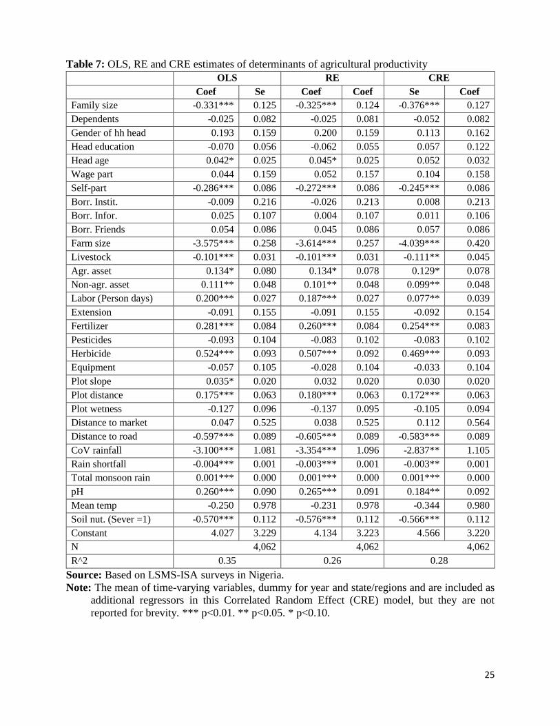
Table 7 reports the estimates of the Cobb-Douglas production function in Equation 3 where

outcome variable is the [ln] value of output per hectare. The first column is from pooled OLS,

13

the second and third columns from random-effects (RE) and correlated random-effects (CRE). As

Correlated Random Effects (CRE) model enables us to address time invariant unobserved

household characteristics and still recover the coefficients on time invariant variables, we will

mainly draw our conclusions based on correlated random-effects estimates.

The results indicate that among the household characteristics, we find that family size

significantly affect land productivity. The estimates also show the presence of an inverse relation

between land size and land productivity which is consistent with many other findings in the

literature (Carletto et al., 2013; Barrett et al., 2010). The coefficient of land size is robust to all

estimation models. The inverse land size-productivity relation has been mostly explained by

market failures (Barrett, 1996).

Results for non-land wealth indicators such agricultural and non-agricultural asset are also

in line with expectations and with the existing literature. Household with higher agricultural and

non-agricultural assets have higher agricultural productivity, which may indicate that wealthier

households are more able to finance the purchase of their farm technology inputs which is

consistent with the other findings (e.g., Asfaw et al., 2016; Peterman et al., 2011).

As for inputs use, we find that labor allocated to agriculture production measured in terms

of person days has a positive and significant effect on land productivity. The elasticity of land

agricultural productivity to person days devoted to agricultural production is about 11%. Similarly,

fertilizer use and application of herbicide have significantly positive effect on agricultural

productivity. These may suggest that adoption of any of the farm management practices may have

a significant role in increasing agricultural productivity. Our results are consistent with a number

of studies that have demonstrated that the security of input use has substantial effect on the

agricultural performance of farmers (e.g., Ravallion and Datt, 1999; Janvry and Sadoulet, 2010;

Mendola, 2007; Amare et al., 2012). We find no evidence of effect access to extension.

We find the distance to nearest road has a significant negative effect on agricultural

productivity. Distances to roads affect transaction costs and access to information, which in turn

affect agricultural productivity. This result indicates that better infrastructure may help to cut

transaction costs, increasing the likelihood of adoption of market-provided inputs and thus increase

agricultural productivity. The distance of the plot to the dwelling is positive and significant,

contrary to expectation. One would have thought the plots closer to the home would be better

managed and thus more productive.

14

As expected, climate and soil-nutrient variables strongly affect agricultural productivity.

We find that farmers located in EAs where the rainfall variability (CoV) is higher have 32% lower

agricultural productivity, while higher season rainfall levels increase land productivity. This is

because abundant rainfall increases harvests and thus land productivity, consistent with the

findings of Asfaw et al. (2016). Rainfall variability, on the other hand, implies increased risk of

farm technology adoption particularly in liquidity constraint and market failure setting, and thus

reduces production and productivity. The results also show the rainfall shortfall significantly

decrease agricultural productivity. Moreover, severe constraints on soil nutrient availability

significantly decrease agricultural productivity. We find the presence of soils characterized by

higher pH levels (than the average in the sample, about 4.49) is productivity enhancing. This result

is expected since most crops grow in a range of soil types but optimally in a well-drained, moist

loam with a pH of 5.6 to 6.4.

5.2. The impact of agricultural productivity

5.2.1. Impact of agricultural productivity on household welfare growth

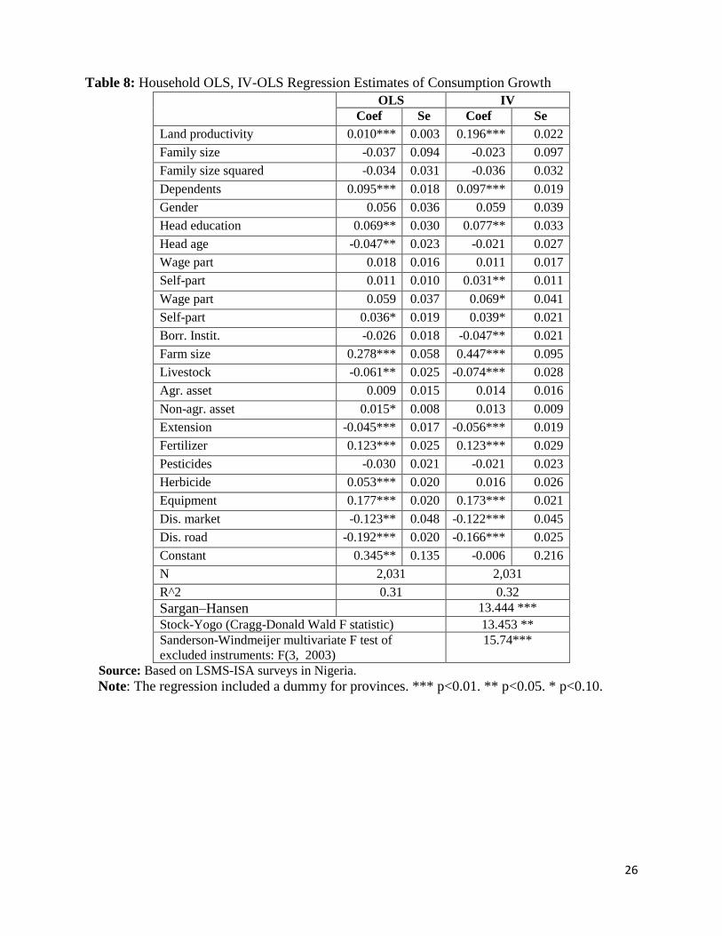
We now turn to an exploration of the impact of agricultural productivity on consumption growth.

The results of the first stage that is used in the later IV analysis to explain asset growth are reported

in the Table 7 in Column 3. All instruments (CoV rainfall, Rain shortfall and Soil nutrient) are

individually and jointly significant at the 5 % level in the first-stage regression, suggesting that the

climate and soil nutrient are crucial factors driving land productivity. We estimate the model for

consumption growth with both OLS, and IV-OLS estimation; the results are reported in Table 8.

Before turning to the causal effects of agricultural productivity on household welfare

growth, we briefly discuss the quality of the selection instruments used. To probe the validity of

our selection instruments, we looked at three major tests: the weak identification test, the relevance

of our instruments and over identification tests. The test results support the choice of the

instruments, as do the F-test values for all of the specifications (bottom of Table 8). The F-statistic

of joint significance of the excluded instruments is greater than 10, thus passing the test for weak

instruments. We use the Sargan–Hansen test of over identifying restrictions and fail to reject the

joint null hypothesis that our instruments are valid instruments. We apply Stock and Yogo to test

weak identification test which is based on the Cragg–Donald Statistic, we reject the null hypothesis

that a given group of instruments is weak against the alternative that it is strong.

15

In general, all model estimates for land productivity are similar in sign; the results obtained

from both models confirm that land productivity has significant, positive effects on consumption

growth. However, the IV estimates for the key variables of interest are much larger than the OLS

estimates, implying that correcting for endogeneity affects the results. Therefore, our subsequent

discussion focuses on the two-stage IV model estimates4.

The results of the IV estimation to examine the impact of the agricultural productivity on

household consumption growth are reported in column (2) of Table 8. The results reveal that

agricultural productivity has a positive, significant impact on consumption growth. Controlling for

other factors, we find that a 10 % increase in the level of agricultural productivity in the previous

year tends to increase consumption growth by 2 % on average. This result supports the hypothesis

that agricultural productivity can facilitate consumption growth by raising the real incomes of

households, and perhaps even indirectly by increasing agricultural outputs which induces job

creation in upstream and downstream non-farm sectors as a response to higher domestic demand.

Households with more dependents experienced a significantly higher consumption growth.

We find that a 10 % increase in years of education of the household head tends to increase

consumption growth by 0.8 % on average. We find non-farm employment opportunities improve

household consumption growth. For example, the effect of non-farm self-employment

participation is particularly strong; consumption growth differs by 3 % between participants and

non-participant households. Similarly both access to formal and informal credit and borrowing

from friends play a significant role in explaining consumption growth. Controlling for other

factors, consumption growth differs by 7 and 4 % between households that have access to

borrowing from formal and informal institutions respectively, compared with those that do not.

Controlling for other factors, we find that households that use fertilizer and farm equipment exhibit

12% and 17%, respectively higher consumption growth as compared households do not use

fertilizer and farm equipment. More important, we find that access to public infrastructure, such

as a nearby market and road, plays a significant role in improving consumption growth.

4 Our results are robust to the use of alternative estimators such as GMM and are available upon request.

Moreover, under the assumptions of conditional homoskedasticity and independence, the efficient GMM

estimator is the traditional IV/2SLS estimator

16

5.2.2. Heterogeneous impact of agricultural productivity

We examine whether the magnitude of the coefficient of agricultural productivity varies by initial

consumption level by estimating the growth model separately for poor and non-poor households.

As is often the case, however, the instruments are not strong as the whole sample for subgroups,

and the F statistic on the excluded instruments is only above 10 for the non-poor households. The

results (Table 9) indicate that agricultural productivity has a positive significant impact on

consumption growth for non-poor and poor households. However, it has a smaller impact on

consumption growth for poor households. Controlling for other factors, we find that a 10 %

increase in agricultural productivity increases consumption growth by 2 % on average for

consumption non-poor households and 0.8 % for poor households. It has is more than two and half

times higher for the non-poor households. The results may suggest that poor smallholder face a

number of constraints that cause to lower their productivity such as lack of information about

production methods and market opportunities, particularly for new crops and varieties prohibit

households from intensifying agriculture and producing high-value commodities whose market

demand is growing rapidly.

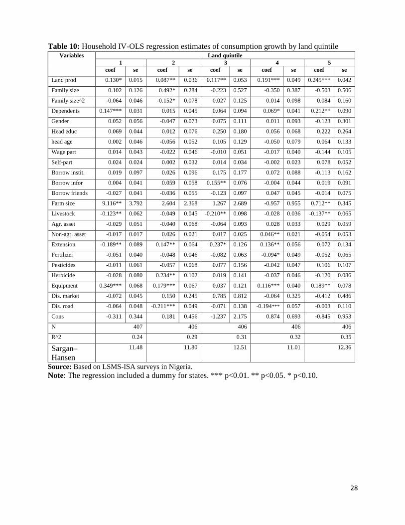
We further allow for heterogeneity in the impact of agricultural productivity by land

holdings. Similar to the wealth status, however, the instruments are not strong as the whole sample

for subgroup (Table 10). The results show that agricultural productivity have a positive significant

impact on consumption growth for all quintiles. However, agricultural productivity have a higher

impact for the household in top two land quintiles compared to the bottom two land quintiles.

When we compare the impact of agricultural productivity for households in the bottom land

quintile and top land quintile, the coefficient for agricultural productivity is approximately two

times higher for the latter. The results may indicate agricultural productivity is not pro-poor, with

the greater gains enjoyed by those who are initially better off. High initial inequality in the

distribution of assets and especially of land may be a plausible candidate in explaining why some

of the agricultural productivity change might be less effective in up lifting poor families from

poverty in developing countries.

6. Conclusions and policy implications

Improving agricultural productivity is widely considered as the most effective means of addressing

poverty and the main pathway out of poverty. However, a key challenge in developing country

17

agriculture is how to increase agricultural productivity to meet food security needs for the growing

population while also reducing poverty of smallholder farmers. Investigating the factors that hinder

or accelerate agricultural productivity, with a particular focus on the role of different measures of

climate variables and soil nutrient data, are priorities in most African national agricultural plans.

Additionally, in this paper we seek to understand whether agricultural productivity, measured

using land productivity, improves household consumption growth using nationally representative

LSMS-ISA panel datasets from Nigeria. We address three important policy questions in the

process of addressing the research objectives. First, what are the main determinants of household

agricultural productivity? Second, how does agricultural productivity impact household welfare

growth? Third, does the relative position of poor people (e.g. the bottom 25%) improve or worsen

with productivity change? Fourth, how do different categories of smallholder farmers benefit from

agricultural productivity?

To address the first objective, we employ the Correlated Random Effects (CRE) model

which involves adding controlling for the household mean of time-varying variables and enables

us to address time invariant unobserved household characteristics and still recover the coefficients

on time invariant variables. We found that the agricultural productivity decreases with family size

and households’ access to non-farm self-employment. The estimates also show the presence of an

inverse relation between land size and land productivity which is consistent with many other

findings in the literature (Carletto et al., 2013; Barrett et al., 2010). We find agricultural and non-

agricultural asset have positive and significant effect on agricultural productivity which may

indicate that wealthier households are more able to finance the purchase of their farm technology

inputs.

We find agricultural productivity increases with increased labor allocated to agriculture

production measured in terms of person days, fertilizer use and the application of herbicide, which

may indicate that input use and farm technology adoption may have a significant role in increasing

agricultural productivity, although we find no evidence of an effect for access to extension

(although this is likely due to limited variability in access). Moreover, we find the distance to

nearest road distance has a significant negative effect on agricultural productivity which suggests

that better infrastructure may help to cut transaction costs increasing the likelihood of adoption of

market-provided inputs and thus increase agricultural productivity. In terms of the impact of

climate and soil-nutrient variables, we find that farmers located in EAs where the rainfall

variability (CoV) is higher have 32% lower agricultural productivity, while higher season rainfall

18

levels increase land productivity. Moreover, severe constraints on soil nutrient availability

significantly decrease agricultural productivity, while we find the presence of soils characterized

by higher pH levels (than the average in the sample, about 4.49) is productivity enhancing.

To provide rigorous evidence of agricultural productivity impact on household welfare

growth and to account for possible endogeneity of agricultural productivity, we applied IV

regression estimation techniques. We find that a 10 % increase in the level of agricultural

productivity in the previous year tends to increase consumption growth by 2 % on average. We

estimate whether the magnitude of the coefficient of agricultural productivity varies by initial

consumption level by estimating the growth model separately for poor and non-poor households.

We find that a 10 % increase in agricultural productivity increases consumption growth by 2 % on

average for consumption non-poor households 0.8 % for poor households. Moreover, we find that

agricultural productivity has a positive significant impact on consumption growth for all land

quintiles. However, productivity have higher impact for the household in top two quintiles.

We believe that our findings have important policy implications for policy makers and

institutions in sub-Saharan Africa at large and in Nigeria in particular. First of all, given the strong

role of farm technology, climate variability, access to infrastructure and assets in improving

agriculture productivity, better targeting agricultural practices to respond to weather risk exposure

and sensitivity, and then building household and system-level capacity to support different

interventions are key factors in improving agricultural productivity. Most importantly, the results

in this article provide very strong arguments on what seem to be required in order to achieve

sustainable pro-poor poverty reduction are integrated interventions that are effective to improve

asset, infrastructure, and use of farm technology and to develop formal insurance markets in order

to enhance the capabilities to smooth agricultural income risk and choices of the poor.

19

References

Arslan, A., Belotti, F., Lipper L. (2016). Smallholder productivity under climatic variability:

Adoption and impact of widely promoted agricultural practices in Tanzania. ESA Working

Paper No. 16-03. Rome, FAO.

Asfaw S., Di Battista, F., Lipper L. (2016). Agricultural Technology Adoption under Climate

Change in the Sahel: Micro-evidence from Niger. Journal of African Economics 1–33

Asfaw, S., Palma, A., Lipper L. (2016). Diversification strategies and adaptation deficit: Evidence

from rural communities in Niger. ESA Working Paper No. 16-02. Rome, FAO.

Barrett, C. B. (2005). Rural poverty dynamics: development policy implications. Agricultural

Economics, 32, 45–60.

Barrett. C., Bellemare, M.F., Hou, J.Y. (2010). Reconsidering Conventional Explanations of the

Inverse Productivity–Size Relationship. World Development Vol. 38, No. 1, pp. 88–97,

2010

Carletto, G., Savastano, S., Zezza, A. (2013). Fact or Artefact: The Impact of Measurement Errors

on the Farm Size-Productivity Relationship. Journal of Development Economics. 103,

254–261

Cervantes-Godoy, D., Dewbre, J. (2010). Economic Importance of Agriculture for Poverty

Reduction. OECD Food, Agriculture and Fisheries Working Papers, No. 23, OECD

Publishing.

Chamberlain, G. (1982). Multivariate regression models for panel data. Journal of Econometrics,

18(1), 5–46.

Christiaensen, L., & Demery, L. (2007). Down to Earth Agriculture and Poverty Reduction in

Africa. The World Bank Group.

Collier, P., Dercon, S. (2014). African agriculture in 50 years: Smallholders in a rapidly changing

world? World Development, 63, 92–101.

Datt, G., M. Ravallion. (1998). “Farm Productivity and Rural Poverty in India.” Journal of

Development Studies 34 (4): 62-85.

de Janvry A., Sadoulet E. (2010). Agricultural growth and poverty reduction: additional evidence.

World Bank Research Observer 25(1), 1–20.

Gollin, D., Lagakos, D., Waugh, M. E. (2014). Agricultural productivity di

erences across countries. The American Economic Review: Papers and Proceedings,

104(5):165-170.

20

Gollin, Douglas, Stephen Parente, and Richard Rogerson. 2002. “The Role of Agriculture in

Development.” American Economic Review 92: 160–64.

Hasan R., Quibria, M.G. (2004). Industry matters for poverty: a critique of agricultural

fundamentalism. Kyklos 57(2), 253–264.

Irz X., Tiffin, R. (2006). “Is Agriculture the Engine of Growth?” Agricultural Economics Journal.

35(1): 79–89.

Liverpool-Tasie S, Olaniyan, B., Salau, S., Sackey, J. (2010). A Review of Fertilizer Policy Issues

in Nigeria. IFPRI NSSP Working Paper 0019. Abuja: IFPRI-Abuja.

Liverpool-Tasie, L., Kuku, O., Ajibola, A. (2011). A Review of Literature on Agricultural

Productivity, Social Capital and Food Security in Nigeria. Nigeria Strategy Support

Program Working Paper 21. Washington, DC: International Food Policy Research

Institute.

Loayza N.V., Raddatz C. (2010). The composition of growth matters for poverty alleviation.

Journal of Development Economics 93(1), 137–151.

Mellor, J.W. (2001). “Faster more equitable growth – agriculture, employment multipliers and

poverty reduction.” Agricultural Policy Development Project Research Report 4,

Cambridge, MA.

Mogues, T., Yu, B., Fan, S., McBride, L. (2012). The Impacts of Public Investment in and for

Agriculture: Synthesis of the Existing Evidence. IFPRI Discussion Paper 1217.

Washington, DC: International Food Policy Research Institute.

Mundlak, Y. (1978). On the pooling of time series and cross section data. Econometrica, 46(1),

69–85.

Oseni, G., McGee, K., Dabalen, A. (2014). Can Agricultural Households Farm Their Way out of

Poverty Development Research Group Poverty and Inequality Team WPS7093

Oseni, G., Winters, P. (2009). Rural nonfarm activities and agricultural crop production in Nigeria.

Agricultural Economics 40(2), 189–201.

Peterman A., Quisumbing A., Behrman J., Nkonya E. (2011) ‘Understanding the Complexities

Surroundings Gender Differences in Agricultural Productivity in Nigeria and Uganda’,

Journal of Development Studies, 47 (10): 1482–509.

Phillip, D., Nkonya, E., Pender, J., Oni, O. A. (2009). Constraints to Increasing Agricultural

Productivity in Nigeria: A Review. IFPRI-NSSP Background Paper 6.

21

Ravallion, M. (2011). On multidimensional indices of poverty. Journal of Economic Inequality

9(2), 235–248.

Ravallion, M., Datt, G. (1996). “How Important to India’s Poor Is the Sectoral Composition of

Economic Growth?” World Bank Economic Review 10 (1):1–25.

Ravallion, M., Datt, G. (1999). “When Is Growth Pro-Poor? Evidence from the Diverse

Experiences of India’s States.” Policy Research Working Paper 2263, World Bank,

Washington, DC.

Smith, J., Barau, A.D., Goldman, A., Mareck, J.H. (1994). the role of technology in agricultural

intensification: The evolution of maize production in the northern Guinea savannah of

Nigeria. Economic Development and Cultural Change 42 (3): 537–554.

Thirtle, C., Lin, L., J. Piesse. (2003). “The impact of research-led agricultural productivity growth

on poverty reduction in Africa, Asia and Latin America.” World Development 31, 1959–

1975.

Timmer, P., Akkus, S. (2008). “The Structural Transformation as a Pathway Out of Poverty:

Analytics, Empirics and Politics” Working Paper 150. Washington, DC: Center for Global

Development

Wooldridge, J. (2010). Econometric analysis of cross section and panel data (2nd ed.). Cambridge,

Mass: MIT Press

World Bank (2014). World Development Indicators 2014. Washington, DC.

http://data.worldbank.org/data-catalog/world-development-indicators.

22

Table 1: Land productivity by land and consumption quintile

Land productivity a distribution

by land quintile

Land productivity distribution by

aggregate consumption quintile

1 826.24 1 346.93

2 482.74 2 523.71

3 430.24 3 500.55

4 327.95 4 424.46

5 235.00 5 507.83

Source: Based on LSMS-ISA surveys in Nigeria.

Note: a Total value of harvested crops (LU, 1000) per hectare

Table 2: Land productivity by land and consumption quintile (N in parentheses)

Land quintile Consumption Quintile

1 2 3 4 5

1 740.27 1010.54 1114.57 1083.68 522.75

(106) (118) (168) (192) (230)

2 364.76 801.092 493.88 349.95 314.39

(174) (188) (180) (116) (154)

3 419.51 384.65 427.08 286.27 659.63

(200) (182) (132) (154) (144)

4 175.43 245.76 348.58 199.35 807.34

(192) (170) (148) (172) (130)

5 161.11 283.23 121.37 109.02 284.18

(142) (154) (184) (178) (154)

Table 3: Land productivity and aggregate consumption by regions

North-

Central

North-

East

North-

West

South-

East

South-

South

South-

West

Land productivity a 385.63 321.05 436.64 474.81 1180.84 286.86

Consumption/AEU 103.34 111.83 84.20 100.27 124.73 138.42

Poverty headcount 0.29 0.23 0.24 0.19 0.11 0.08

N 782 828 1082 886 304 180

Source: Based on LSMS-ISA surveys in Nigeria.

Note: a Total value of harvested crops (LU, 1000) per hectare

23

Table 4: Household aggregate consumption per AEU by consumption quintile and year

Consumption quintile 2010 2012 % change

1 46.84 40.53 -0.13

2 76.10 62.89 -0.17

3 100.55 83.49 -0.17

4 132.12 105.09 -0.21

5 216.65 160.62 -0.26

Source: Based on LSMS-ISA surveys in Nigeria.

Note: aTotal value of harvested crops (LU, 1000) per hectare

Table 5: OLS regression of climate variables and soil nutrients on land productivity (UNITS)

Coef Se

CoV of annual rainfall -5.343*** 1.534

Total monsoon rainfall(mm) 0.001** 0.000

Rain shortfall(mm) -0.001** 0.001

Soil nutrient(Sever constraint=1) -0.335*** 0.120

pH -0.888 0.644

Mean temperature -1.568* 0.918

Constant 9.776*** 3.615

State fixed effects Yes Y

N 4,062

Source: Based on LSMS-ISA surveys in Nigeria.

Note: State fixed effects are included in the specifications. *** p<0.01. ** p<0.05. * p<0.10.

24

Table 6: Description and Summary Statistics Variable Description All 2010 2012

N=4062 N=2031 N=2031

Mean Std.

Dev.

Mean Std.

Dev.

Mean Std.

Dev.

Consumption Aggregate consumption per AEU (local

unit=LU, 1000)

102.59 66.03 114.62 68.52 90.56 61.14

Value harvest Total value of harvested crops (LU, 1000) 134.14 619.24 122.60 532.74 145.68 1227.35

Land prod. Land productivity= (total value of

harvested per hectare)

460.64 1955 608.21 2268.34 313.06 1569.37

Household characteristics

Family size Family size (adult equivalent unit ) 5.41 2.07 5.14 1.95 5.68 2.15

Dependents Dependent (<15 , >64 years old) 3.24 2.28 3.31 2.30 3.18 2.26

Gender Gender of the household head 0.89 0.31 0.89 0.31 0.88 0.32

Head educ Educ. HH head ( years ) 4.47 4.72 4.60 4.69 4.34 4.75

Head age Age HH head (years ) 51.00 15.05 49.71 15.04 52.28 14.96

Borr. instit. Borrowing from formal institutions 0.03 0.18 0.03 0.16 0.04 0.21

Borr. infor. Borrowing from informal institutions 0.20 0.40 0.20 0.40 0.20 0.40

Borr. friends Borrowing from friends 0.30 0.46 0.30 0.46 0.30 0.46

Wage part Wage labor employment participation 0.07 0.26 0.02 0.13 0.13 0.33

Self-part Non-farm self-employment participation 0.52 0.50 0.49 0.50 0.55 0.50

Wealth indicators

Farm size Farm size (in hectare ) 0.59 0.93 0.62 0.98 0.56 0.85

Livestock Total livestock -Tropical livestock unit 78.65 1142.10 23.37 924.99 133.92 1322.02

Agr. asset Value of agricultural assets (LU, 10^) 82.50 528.00 45.17 270.10 119.82 1564.97

Non-agr. asset Value of total non-agricultural asset (LU,

1000)

562.76 2464.56 648.28 3372.40 477.24 873.71

Farm Inputs

Person days Labor (both family & hired labor)

allocated to agricultural production person

days

198.79 239.65 206.47 243.24 191.10 235.93

Extension Access to extension (yes=1) 0.10 0.27 0.11 0.26 0.10 0.27

Fertilizer Fertilizer use indicator(yes=1) 0.48 0.50 0.48 0.50 0.48 0.50

Pesticides Pesticides use indicator(yes=1) 0.19 0.39 0.18 0.38 0.20 0.40

Herbicide Herbicide use indicator(yes=1) 0.27 0.44 0.24 0.43 0.29 0.45

Equipment Equipment use indicator(yes=1) 0.23 0.42 0.21 0.41 0.24 0.43

Plot distance Plot distance(km) 3.71 44.30 6.01 61.31 1.41 12.54

Plot wetness Plot potential wetness index 14.37 3.60 14.08 4.18 14.66 2.88

Plot slope Plot slope 2.83 2.74 2.78 2.98 2.88 2.49

Market Distance to the market (km) 69.71 37.71 69.74 37.69 69.68 37.74

Road Distance to the road (km) 13.22 15.11 18.44 18.43 8.00 7.93

Climate and bio-physical variables

CV rainfall CoV rainfall (1983-2012) (average/15Km

EA radius)

0.22 0.05 0.22 0.05 0.22 0.05

Rain shortfall Average rain shortfall (1983-2012)

(avg/15Km EA radius)

89.37 62.84 114.18 74.98 64.57 32.34

Season rainfall Season total rainfall(mm) 886.17 236.70 937.55 244.38 834.80 216.97

Soil nutrient Soil nutrient avail (Severe contraints) 0.25 0.44

pH Soil pH (avg/15Km EA radius) 4.49 0.58

Temperature Season average temp(1990-2012)

(avg/15Km EA radius)

25.63 1.21 25.56 1.22 25.70 1.21

Source: Based on LSMS-ISA surveys in Nigeria.

25

Table 7: OLS, RE and CRE estimates of determinants of agricultural productivity

OLS RE CRE

Coef Se Coef Coef Se Coef

Family size -0.331*** 0.125 -0.325*** 0.124 -0.376*** 0.127

Dependents -0.025 0.082 -0.025 0.081 -0.052 0.082

Gender of hh head 0.193 0.159 0.200 0.159 0.113 0.162

Head education -0.070 0.056 -0.062 0.055 0.057 0.122

Head age 0.042* 0.025 0.045* 0.025 0.052 0.032

Wage part 0.044 0.159 0.052 0.157 0.104 0.158

Self-part -0.286*** 0.086 -0.272*** 0.086 -0.245*** 0.086

Borr. Instit. -0.009 0.216 -0.026 0.213 0.008 0.213

Borr. Infor. 0.025 0.107 0.004 0.107 0.011 0.106

Borr. Friends 0.054 0.086 0.045 0.086 0.057 0.086

Farm size -3.575*** 0.258 -3.614*** 0.257 -4.039*** 0.420

Livestock -0.101*** 0.031 -0.101*** 0.031 -0.111** 0.045

Agr. asset 0.134* 0.080 0.134* 0.078 0.129* 0.078

Non-agr. asset 0.111** 0.048 0.101** 0.048 0.099** 0.048

Labor (Person days) 0.200*** 0.027 0.187*** 0.027 0.077** 0.039

Extension -0.091 0.155 -0.091 0.155 -0.092 0.154

Fertilizer 0.281*** 0.084 0.260*** 0.084 0.254*** 0.083

Pesticides -0.093 0.104 -0.083 0.102 -0.083 0.102

Herbicide 0.524*** 0.093 0.507*** 0.092 0.469*** 0.093

Equipment -0.057 0.105 -0.028 0.104 -0.033 0.104

Plot slope 0.035* 0.020 0.032 0.020 0.030 0.020

Plot distance 0.175*** 0.063 0.180*** 0.063 0.172*** 0.063

Plot wetness -0.127 0.096 -0.137 0.095 -0.105 0.094

Distance to market 0.047 0.525 0.038 0.525 0.112 0.564

Distance to road -0.597*** 0.089 -0.605*** 0.089 -0.583*** 0.089

CoV rainfall -3.100*** 1.081 -3.354*** 1.096 -2.837** 1.105

Rain shortfall -0.004*** 0.001 -0.003*** 0.001 -0.003** 0.001

Total monsoon rain 0.001*** 0.000 0.001*** 0.000 0.001*** 0.000

pH 0.260*** 0.090 0.265*** 0.091 0.184** 0.092

Mean temp -0.250 0.978 -0.231 0.978 -0.344 0.980

Soil nut. (Sever =1) -0.570*** 0.112 -0.576*** 0.112 -0.566*** 0.112

Constant 4.027 3.229 4.134 3.223 4.566 3.220

N 4,062 4,062 4,062

R^2 0.35 0.26 0.28

Source: Based on LSMS-ISA surveys in Nigeria.

Note: The mean of time-varying variables, dummy for year and state/regions and are included as

additional regressors in this Correlated Random Effect (CRE) model, but they are not

reported for brevity. *** p<0.01. ** p<0.05. * p<0.10.

26

Table 8: Household OLS, IV-OLS Regression Estimates of Consumption Growth

OLS IV

Coef Se Coef Se

Land productivity 0.010*** 0.003 0.196*** 0.022

Family size -0.037 0.094 -0.023 0.097

Family size squared -0.034 0.031 -0.036 0.032

Dependents 0.095*** 0.018 0.097*** 0.019

Gender 0.056 0.036 0.059 0.039

Head education 0.069** 0.030 0.077** 0.033

Head age -0.047** 0.023 -0.021 0.027

Wage part 0.018 0.016 0.011 0.017

Self-part 0.011 0.010 0.031** 0.011

Wage part 0.059 0.037 0.069* 0.041

Self-part 0.036* 0.019 0.039* 0.021

Borr. Instit. -0.026 0.018 -0.047** 0.021

Farm size 0.278*** 0.058 0.447*** 0.095

Livestock -0.061** 0.025 -0.074*** 0.028

Agr. asset 0.009 0.015 0.014 0.016

Non-agr. asset 0.015* 0.008 0.013 0.009

Extension -0.045*** 0.017 -0.056*** 0.019

Fertilizer 0.123*** 0.025 0.123*** 0.029

Pesticides -0.030 0.021 -0.021 0.023

Herbicide 0.053*** 0.020 0.016 0.026

Equipment 0.177*** 0.020 0.173*** 0.021

Dis. market -0.123** 0.048 -0.122*** 0.045

Dis. road -0.192*** 0.020 -0.166*** 0.025

Constant 0.345** 0.135 -0.006 0.216

N 2,031 2,031

R^2 0.31 0.32

Sargan–Hansen 13.444 ***

Stock-Yogo (Cragg-Donald Wald F statistic) 13.453 **

Sanderson-Windmeijer multivariate F test of

excluded instruments: F(3, 2003)

15.74***

Source: Based on LSMS-ISA surveys in Nigeria.

Note: The regression included a dummy for provinces. *** p<0.01. ** p<0.05. * p<0.10.

27

Table 9: Household IV-OLS Regression Estimates of Consumption Growth by Welfare Status

Poor Non-poor

Coef Se Coef Se

Land prod 0.083** 0.045 0.202*** 0.028

Family size 0.095 0.701 -0.038 0.115

Family size^2 -0.126 0.204 -0.037 0.040

Dependents 0.078 0.063 0.115*** 0.025

Gender -0.158 0.100 0.102** 0.049

Head educ 0.090 0.178 0.088** 0.041

head age -0.094 0.087 -0.007 0.040

Wage part 0.044 0.049 0.012 0.020

Self-part -0.060 0.048 0.027* 0.014

Borrow institutional 0.077 0.255 0.068 0.051

Borrow informal -0.100 0.076 0.038 0.027

Borrow friends 0.054 0.087 -0.031 0.025

Farm size -1.042* 0.601 0.510*** 0.106

Livestock -0.065 0.074 -0.047 0.029

Agricultural asset 0.102** 0.047 -0.033 0.021

Non-agricultural asset 0.151** 0.062 0.013 0.011

Extension 0.293** 0.131 0.127*** 0.035

Fertilizer 0.097 0.063 -0.087*** 0.024

Pesticides -0.277** 0.115 -0.006 0.027

Herbicide 0.278*** 0.106 -0.008 0.032

Equipment 0.176** 0.071 0.189*** 0.026

Dis. market -0.526 0.411 -0.164*** 0.060

Dis. road -0.299*** 0.062 -0.118*** 0.032

Cons 1.536* 0.837 -0.342 0.298

N 450 1,581

R^2 0.34 0.31

Sargan–Hansen 10.50 13.00

Source: Based on LSMS-ISA surveys in Nigeria.

Note: The regression included a dummy for states. *** p<0.01. ** p<0.05. * p<0.10.

28

Table 10: Household IV-OLS regression estimates of consumption growth by land quintile Variables Land quintile

1 2 3 4 5

coef se coef se coef se coef se coef se

Land prod 0.130* 0.015 0.087** 0.036 0.117** 0.053 0.191*** 0.049 0.245*** 0.042

Family size 0.102 0.126 0.492* 0.284 -0.223 0.527 -0.350 0.387 -0.503 0.506

Family size^2 -0.064 0.046 -0.152* 0.078 0.027 0.125 0.014 0.098 0.084 0.160

Dependents 0.147*** 0.031 0.015 0.045 0.064 0.094 0.069* 0.041 0.212** 0.090

Gender 0.052 0.056 -0.047 0.073 0.075 0.111 0.011 0.093 -0.123 0.301

Head educ 0.069 0.044 0.012 0.076 0.250 0.180 0.056 0.068 0.222 0.264

head age 0.002 0.046 -0.056 0.052 0.105 0.129 -0.050 0.079 0.064 0.133

Wage part 0.014 0.043 -0.022 0.046 -0.010 0.051 -0.017 0.040 -0.144 0.105

Self-part 0.024 0.024 0.002 0.032 0.014 0.034 -0.002 0.023 0.078 0.052

Borrow instit. 0.019 0.097 0.026 0.096 0.175 0.177 0.072 0.088 -0.113 0.162

Borrow infor 0.004 0.041 0.059 0.058 0.155** 0.076 -0.004 0.044 0.019 0.091

Borrow friends -0.027 0.041 -0.036 0.055 -0.123 0.097 0.047 0.045 -0.014 0.075

Farm size 9.116** 3.792 2.604 2.368 1.267 2.689 -0.957 0.955 0.712** 0.345

Livestock -0.123** 0.062 -0.049 0.045 -0.210** 0.098 -0.028 0.036 -0.137** 0.065

Agr. asset -0.029 0.051 -0.040 0.068 -0.064 0.093 0.028 0.033 0.029 0.059

Non-agr. asset -0.017 0.017 0.026 0.021 0.017 0.025 0.046** 0.021 -0.054 0.053

Extension -0.189** 0.089 0.147** 0.064 0.237* 0.126 0.136** 0.056 0.072 0.134

Fertilizer -0.051 0.040 -0.048 0.046 -0.082 0.063 -0.094* 0.049 -0.052 0.065

Pesticides -0.011 0.061 -0.057 0.068 0.077 0.156 -0.042 0.047 0.106 0.107

Herbicide -0.028 0.080 0.234** 0.102 0.019 0.141 -0.037 0.046 -0.120 0.086

Equipment 0.349*** 0.068 0.179*** 0.067 0.037 0.121 0.116*** 0.040 0.189** 0.078

Dis. market -0.072 0.045 0.150 0.245 0.785 0.812 -0.064 0.325 -0.412 0.486

Dis. road -0.064 0.048 -0.211*** 0.049 -0.071 0.138 -0.194*** 0.057 -0.003 0.110

Cons -0.311 0.344 0.181 0.456 -1.237 2.175 0.874 0.693 -0.845 0.953

N 407 406 406 406 406

R^2 0.24 0.29 0.31 0.32 0.35

Sargan–

Hansen

11.48 11.80 12.51 11.01 12.36

Source: Based on LSMS-ISA surveys in Nigeria.

Note: The regression included a dummy for states. *** p<0.01. ** p<0.05. * p<0.10.