The impact of central bank FX interventions on currency

components∗

Michel BEINE†, Charles S. BOS‡and Sebastien LAURENT§

September 4 2006

Abstract

This paper is the first attempt to assess the impact of official FOREX interventionsof the three major central banks in terms of the dynamics of the currency componentsof the major exchange rates (EUR/USD and YEN/USD) over the period 1989-2003. Weidentify the currency components of the mean and the volatility processes of exchangerates using the recent Bayesian framework developed by Bos and Shephard (2006). Ourresults show that in general, the concerted interventions tend to affect the dynamics ofboth currency components of the exchange rate. In contrast, unilateral interventions arefound to primarily affect the currency of the central bank present in the market. Ourfindings also emphasize a role for interventions conducted by these central banks on otherrelated FOREX markets.

∗This paper has benefited from useful comments and particular suggestions of V. Bodart, B. Candelon,G. Chortareas, E. Girardin, C. Neely, G. Prat and from participants of conferences in Aarhus, New York,Luxembourg, Strasbourg and Maastricht. Of course, the usual disclaimer applies.

†University of Luxemburg (Luxemburg) and CES Ifo; michel.beine@uni.lu.‡Tinbergen Institute and Vrije Universiteit Amsterdam (The Netherlands); cbos@feweb.vu.nl.§University of Namur and CORE (Belgium); sebastien.laurent@fundp.ac.be.

1 Introduction

The use of direct interventions in the FX market remains a stabilisation instrument in thehand of the central banks of the major industrialised countries. While the Federal Reserve(Fed hereafter) has been increasingly reluctant to rely on such interventions since 1995, theother major central banks have recently been involved in such a policy. In 2000, the EuropeanCentral Bank (ECB) conducted a round of sales of foreign currency aimed at supporting theEuro (EUR) against the US Dollar (USD). In recent years, the Bank of Japan (BoJ) has beenextremely active in the FX markets, proceeding to massive sales of its currency against boththe USD and the Euro. As a piece of evidence, over the year 2003 only, the BoJ was presentin the markets during 82 business days and purchased more than 20 billions of USD.

Given the extensive use of these central bank interventions (CBIs), a large empiricalliterature has tried to assess their efficiency, both in terms of exchange rate level and volatility.Due to the release of the official data by the three major central banks, most analyses haverelied on the financial econometric approaches based on daily and even intra-daily data.Extensive reviews of this literature are provided among others by Sarno and Taylor (2001)and Humpage (2003). On the whole, the literature sheds some doubt about the efficiency ofthis instrument. While little evidence has been found that direct sales or purchases of foreigncurrency succeed in driving the exchange rate in the desired direction, most studies using highfrequency (weekly, daily or intra-daily) data conclude that such operations result in increasedexchange rate volatility. Another robust finding emphasises that while concerted operationstend to move the market, unilateral interventions exert some limited impact on the dynamicsof exchange rates.

Explanations of the empirical results have been provided mainly by referring to the sig-nalling theory. The signalling channel (Mussa 1981) states that by intervening, the centralbanks convey some private information about fundamentals to market participants and there-fore tend to alter their expectations in terms of future values of the exchange rate. Such atheory stresses the case for potential asymmetric effects of interventions depending on their in-trinsic features. In this respect, an important distinction concerns unilateral versus concertedoperations. Along the signalling hypothesis, interventions carried out by a single central bankshould mainly affect the dynamics of the currency of the central bank present in the market.In contrast, concerted interventions should be seen more as market-wide events that can af-fect the value of both currencies. Testing for the existence of such asymmetric effects is theprimary aim of this paper.

We revisit the analysis of the short-run impact of CBIs conducted by the major centralbanks (the US Fed, the ECB, or Bundesbank (BB) before the introduction of the Euro, andthe BoJ) in the foreign exchange market over the recent period (1989-2003). Unlike the restof the literature, we focus on the impact on the currency components of the exchange ratesrather than on the exchange rate itself. The level and the volatility of these (unobserved)currency components are identified using the recent Bayesian modelling approach proposedby Bos and Shephard (2006). This approach extends the early development of Mahieu andSchotman (1994) and involves the estimation of a state-space model with a series of stochasticcurrency level and volatility processes. Our analysis allows to express each exchange rate asthe combination of two unobserved currency factors whose moments can be investigated alongwith the CBIs taking place in the market.

In short, the central issue of interest is the possible asymmetry of CBIs in terms ofvolatility. We also study the existence of a dollar bias in the effects of interventions and the

2

importance of FX operations in auxiliary markets for the analysis. The assessment of thesetwo last points can be seen as an interesting by-product of our analysis in terms of currencyfactors.

On the whole, our results support the existence of asymmetric effects between unilateraland concerted operations. We find that while coordinated operations affect the volatility ofboth currencies, unilateral interventions lead to an increase only in the currency componentof the central bank present in the market. The traditional analysis in terms of exchangerates turns out to be unable to isolate this last effect. With the alternative identificationin terms of currency components we show that limited, unilateral operations can still influ-ence the currency volatility significantly. To the extent that a rise in uncertainty might beconsidered detrimental, this finding suggests that even unilateral interventions yield somecounterproductive results.

The paper is organised as follows. Section 2 reviews the empirical literature on the impactof CBIs and clarifies the nature of our contribution. Section 3 presents both the model and theestimation procedure, comments on the extracted country specific components and providessome insight on the quality of the volatility measures of the extracted currency components.Section 4 details our empirical approach, provides the findings and interprets the results.It also assesses the robustness of the results to some alternative specification. Section 5summarises the conclusions, and points the way for future extensions of this research project.

2 The state of the literature and contribution of the paper

2.1 Previous empirical findings

The release of high frequency data on their FX interventions by the major central banks hasinduced the development of an extensive empirical literature aimed at capturing the impact ofsuch operations on the dynamics of exchange rates. Recent work including Sarno and Taylor(2001), Humpage (2003), Dominguez (2004) or ? has fortunately provided some reviews ofthis large literature. Different econometric approaches have been proposed to capture theeffects of CBIs, including event studies and parametric models. Due to emphasis on theimpacts in terms of exchange rate uncertainty, different approaches to measure volatility havebeen used: GARCH models (Dominguez 1998), implied volatility modelling (Bonser-Neal andTanner 1996, Beine 2004) or more recently realised volatility (Beine, Laurent and Palm 2004).While the bulk of the empirical analyses has studied the impact using daily data, some recentapproaches have investigated the impact in an intra-daily perspective (Dominguez 2003, Payneand Vitale 2003).

As emphasised by several authors, there is no clear consensus in the literature concerningthe efficiency of these CBIs. While Dominguez (2003) and Payne and Vitale (2003) find somerobust effects of CBIs in the very short run on the level of exchange rate returns, most studiesconducted at the daily frequency find either insignificant or mixed results.1 The results interms of exchange rate volatility seem much more clear-cut, pointing out that in general,direct interventions tend to raise exchange rate volatility. This holds for daily data although

1A number of papers (see among others Beine, Benassy-Quere and Lecourt 2002) document even perverseeffects on the returns. These perverse effects have been rationalised by some theoretical contributions empha-sising the role of the interaction process between the central bank and the market traders (Bhattacharya andWeller 1997).

3

some recent evidence (Dominguez 2003, Beine et al. 2004) find that these volatility effectsmight be mean reverting within a couple of hours.

Another feature of this empirical literature is that the results tend to be dependent onthe involved currency markets as well as on the sample period under investigation. This ishardly surprising given that exchange rate policies vary over time and across central banks.As an example, while the ECB and the Federal Reserve have been increasingly reluctant tointervene in the FX markets after 1995, the BoJ activity in the FX markets has reached apeak in 2003. As another example, while the BoJ tended to use a transparent policy before2003, it might have recently favoured secret interventions (Beine and Lecourt 2004).

Most of these empirical findings concerning the effects of official interventions have beenrationalised using the signalling theory (Mussa 1981). The interventions under investigationhave been reported by the central banks to be sterilised, which rules out any monetary channel.The portfolio channel has also received very little support, which is understandable given therelatively small amounts used by the central banks in these operations.2 The signalling theorystates that through these interventions, central banks convey some fundamental informationabout their future policies. Along the signalling channel, the unilateral interventions carriedout by a central bank should signal private information mainly useful to assess the futurevalue of its currency. There is much less rationale that such operations aims at conveyingany valuable information relative to the other currencies. In this respect, our analysis whichdisentangles the impact of CBIs into currency components provides a useful way to test furtherthe signalling channel as the main channel at work to explain their effects.

2.2 Contribution of the paper

The general contribution of this paper is to focus on the impact of interventions on thecurrency dynamics rather that on the exchange rate evolution. There are three main reasonscalling for the adoption of an analysis in terms of currency components. In turn, this approachenables to provide answers to three specific questions concerning the impact of CBIs in theFX markets.

First, unlike certain financial events like oil price increases, foreign exchange CBIs are bydefinition country specific or geographical area specific events. For instance, a sale of JapaneseYen (YEN) by the Bank of Japan is expected to impact primarily the value of the Yen againstall the currencies, especially when such operations are not concerted, i.e. when they involvea single central bank. This idea is consistent with the popular flexible-price monetary model(Frenkel 1976) in which the value of the nominal exchange rate is related to the difference offuture expected values of domestic and foreign variables such as the money stock, output andinterest rates. Depending on whether these CBIs are unilateral or concerted the signallingcontent about these variables will be different, inducing therefore a different impact on thedynamics of the exchange rate.

The statistical investigation in terms of currencies or country components rather thanin terms of exchange rates can therefore shed interesting light on particular effects of theseCBIs and on asymmetric effects associated to different types of operations. Basically, theempirical literature finds less impact of unilateral rather than concerted operations, especially

2A notable exception is Evans and Lyons (2005). Their analysis nevertheless applies to primarily secret in-terventions, i.e. unreported official interventions which represent a rather small proportion of the interventionscarried out by the three major central banks over this period.

4

in terms of volatility.3 Using our dataset (see later) and relying on a standard EGARCHspecification which is representative of the existing literature, we find results highly consistentwith these findings. For the sake of brevity, these findings are reported in Appendix D. Tosummarise, over the 1989-2003 period, we find (i) that most significant effects concern thevolatility part, (ii) coordinated interventions unambiguously increase exchange rate volatilityand (iii) unilateral interventions affects volatility in a much more moderate way. Given thedifferentiated content carried out by these operations, one reason for this result could bethat an intervention from a given central bank will mostly impact the country component ofthe exchange rate of the active central bank, without much effect on the component of thecounterpart country. Testing for such an effect is only possible after some clear identificationof the currency component. In a nutshell, we try to answer the following question:

Question 1 Is there some evidence of asymmetric effects between unilateral and concerted

operations in terms of currency dynamics?

Second, most analyses of CBIs conducted in the context of flexible exchange rate regimesinvolve the USD currency. When it comes to CBIs, this choice is a natural one because thedollar is often the currency against which foreign central banks try to stabilise the value oftheir currency. Furthermore, the investigation of the USD allows to make a clear distinctionbetween coordinated and unilateral operations.4 Once more, such a distinction stems fromthe different signalling content conveyed by these two types of interventions. While the choiceof the USD is rational, it might nevertheless be dangerous to draw general conclusions on theimpact of these interventions, given the special situation of the USD as the world leadingcurrency. The USD is by far the most liquid currency, especially for spot transactions.5

Detken and Hartman (2000) discuss the various features involving the international role ofcurrencies (financing and investment roles), with a special emphasis on the changes associatedwith the inception of the Euro. They document the leading position of the USD in allsegments, especially during the period before 1999 in which the Fed and the Bundesbankwere active on the markets. Disentangling the impact in terms of currencies rather than interms of exchange rates might therefore be useful to assess the part of the results related tothe special situation of the USD. In other words, we address the second following question:

Question 2 Is there a dollar effect driving the empirical results regarding the effects of CBIs?

A third and important contribution is the way one controls for what is called auxiliaryinterventions in the FX markets. Auxiliary interventions are interventions involving a partic-ular currency but occurring on another market. Infra-marginal interventions in the contextof the European Monetary System (EMS) provide a good example of these auxiliary inter-ventions.6 The massive sales of Deutsche Mark (DEM) by the Bundesbank against some

3See among others Dominguez (1998) and Beine et al. (2004). It should be emphasised that while theimpact of unilateral interventions is generally lower than the one obtained for concerted operations, it hasbeen found to be statistically significant for some of these operations.

4Basically, the YEN/USD and the EUR/USD markets are the only liquid markets on which concertedinterventions have taken place over the recent period. A given intervention is considered as concerted if it iscarried out by the two involved central banks the same day and in the same direction. Such a situation ispartly due to the strategy of the Fed favouring these two important markets.

5The triennial survey on FX markets conducted by the Bank for International Settlements (BIS, 2001)shows that over the 1989-2001, the USD entered on average on one side of 86.6% of all foreign exchangetransactions, against 38 and 23.48% for the Euro and the YEN, respectively. The 2004 survey yields verysimilar figures.

6The other case considered in this paper concerns unilateral YEN sales of the BoJ against the Euro.

5

European currencies (like the Italian Lira, the Spanish Peseta or the French Frank) duringthe 1992/3 EMS crisis might have impacted the DEM against the USD. However, while itis tedious to find a clear rationale for introducing these interventions in a classical exchangerate equation of the DEM/USD, it is more straightforward to allow for some impact on theDEM currency component. In turn, this ensures a better control for other type of news inthe model and hence a better estimation of these CBI effects. Our analysis therefore aims atanswering a third question:

Question 3 Should one account for interventions on auxiliary markets when analysing the

impact of FX operations in the major markets?

3 Modelling exchange rates in factors

3.1 Exchange rate data

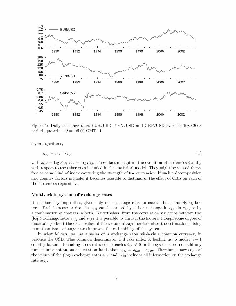
Our dataset contains hourly data for three major exchange rates (four currencies), theJapanese Yen, the Euro (with corresponding Deutsche Mark value before the introductionof the Euro in 1999) and the British Pound (GBP) against the US Dollar. For these threeexchange rates, we have about 14.5 years of intraday (hourly) data, from January 1 1989 toMay 31 2003. The raw data consists of all interbank EUR/USD, YEN/USD and GBP/USDbid-ask quotes displayed on the Reuters FX screen during this period. The series are presentedin Figure 1.

As standard in the literature, we compute hourly exchange rate prices St,ij(Q) at time t,quoted at hour Q = 0, . . . , 23 GMT+1 between currencies i and j from the linearly interpo-lated average of the logarithms of bid and ask quotes for the two ticks immediately beforeand after the hourly time stamps throughout the global 24-hour trading day. Next we obtaindaily and intradaily returns as the first difference of the logarithmic daily or intradaily prices,multiplied by 100 for ease of presentation whenever convenient.

3.2 The model

Exchange rates

Current models in the exchange rate literature tend to model the exchange rates betweencurrencies i and j at time t St,ij directly, possibly after taking the first difference of itslogarithms.7 For multivariate models, using St,ij and St,ik for countries i, j and k jointly, thisinduces a strong source of correlation, as both exchange rates involve the common currencyi.

Mahieu and Schotman (1994) propose to model each underlying unobserved currencyfactor separately, thus explicitly taking the correlation in exchange rates along. Each exchangerate St,ij (e.g. EUR/USD) at time t between currencies i and j comprises information on thetwo currencies Et,i (e.g. EUR) and Et,j (e.g. USD), as

St,ij =Et,i

Et,j,

7Note that, for ease of presentation, we do not specify the quotation time of the exchange rates in thissection.

6

0.6 0.7 0.8 0.9 1 1.1 1.2 1.3

1990 1992 1994 1996 1998 2000 2002

EUR/USD

75 90

105 120 135 150 165

1990 1992 1994 1996 1998 2000 2002

YEN/USD

0.45 0.5

0.55 0.6

0.65 0.7

0.75

1990 1992 1994 1996 1998 2000 2002

GBP/USD

Figure 1: Daily exchange rates EUR/USD, YEN/USD and GBP/USD over the 1989-2003period, quoted at Q = 16h00 GMT+1

or, in logarithms,

st,ij = et,i − et,j (1)

with st,ij = log St,ij , et,i = log Et,i. These factors capture the evolution of currencies i and jwith respect to the other ones included in the statistical model. They might be viewed there-fore as some kind of index capturing the strength of the currencies. If such a decompositioninto country factors is made, it becomes possible to distinguish the effect of CBIs on each ofthe currencies separately.

Multivariate system of exchange rates

It is inherently impossible, given only one exchange rate, to extract both underlying fac-tors. Each increase or drop in st,ij can be caused by either a change in et,i, in et,j , or bya combination of changes in both. Nevertheless, from the correlation structure between two(log-) exchange rates st,ij and st,kj it is possible to unravel the factors, though some degree ofuncertainty about the exact value of the factors always persists after the estimation. Usingmore than two exchange rates improves the estimability of the system.

In what follows, we use a series of n exchange rates vis-a-vis a common currency, inpractice the USD. This common denominator will take index 0, leading us to model n + 1country factors. Including cross-rates of currencies i, j 6= 0 in the system does not add anyfurther information, as the relation holds that st,ij ≡ st,i0 − st,j0. Therefore, knowledge ofthe values of the (log-) exchange rates st,i0 and st,j0 includes all information on the exchangerate st,ij .

7

Currency factors and volatility

Before the factors can be extracted, a further assumption about the evolution of the underlyingfactors needs to be made. The basic assumption is to allow the factors to evolve according to arandom walk (which implies the assumption of unpredictable returns on the exchange rates),with independent normal disturbances. Stochastic volatility (SV) components (Harvey, Ruizand Shephard 1994, Jacquier, Polson and Rossi 1994) govern the variance of the series. Thecountry factors evolve, at the daily frequency, along the following lines:

et+1,i = βt,i + et,i + ǫt,i, t = 0, . . . , T, (2)

ǫt,i ∼ N (0, exp(ht,i)), i = 0, . . . , n, (3)

ht+1,i − γt+1,i = φi(ht,i − γt,i) + ξt,i, (4)

ξt,i ∼ N (0, σ2ξ,i). (5)

The stochastic volatility specification for the variances of the random walk disturbances allowsfor more flexibility than the standard deterministic GARCH specification (Bos, Mahieu andVan Dijk 2000, Carnero, Pena and Ruiz 2001), as there is an additional element of randomvariation in the model. The drawback of allowing for stochastic volatility however is that theestimation tends to be much more computationally demanding. This seems to be the mainreason that relatively few applications have appeared in the literature.

The assumptions for the country factors imply a random walk structure for the logarithmof the exchange rates as well, with an intricate correlation of first and second moments of theexchange rate returns due to the combination of the country factors for level and volatility.The implied structure for the exchange rates is consistent with the findings of the literatureon the impossibility of predicting the level of exchange rates (certainly at longer horizons),but with clear persistence in the variance.

Note that the model is set up at the daily frequency; in the application the quotation timeof the data is chosen in accordance with the expected timing of the CBI. Moving up towardsan intra-day analysis introduces further complications concerning intra-day seasonality of thevolatilities, and is left for future research.

Interventions

Both the random walk equation (2) and the stochastic volatility equation (4) allow for a timevarying mean βt,i and γt,i to model the baseline mean and variance as well as the effects ofthe interventions of the central banks Wt,i. We model

βt,i = Wt,iβi, (6)

γt,i = γ0i + |Wt,i|γi, (7)

with Wt,i a vector of indicators for the different interventions affecting the currency at timet (see Section 4.1), and β, γ the corresponding vectors of parameters. By convention, theindicators take the value 0 when there is no intervention, -1 or 1 in case of a sale or a purchaseof USD respectively on a specific currency market. For the auxiliary interventions, i.e. thosenot involving the USD, -1 and 1 correspond to the purchase or sale of the own currency by theintervening central bank. The equation for γt,i includes an overall constant γ0i to govern thebaseline variance, and only takes the timing, not the direction, of interventions into account.8

8It was brought to our attention by a referee that instead of this fixed effects (FE) specification for theinterventions, a random effects (RE) specification could be used. Defining gt+1,i − γ0i = φ(gt,i − γ0i) + ξt,i as

8

Disturbances

The disturbances ǫt,i are taken independent across time t and countries i. As exchange ratereturns themselves show little or no autocorrelation, the underlying factor increments canreasonably be assumed independent across time.

The independence across countries is a different issue. One can imagine that a global crisishas a negative effect on all or some currencies jointly. Tims and Mahieu (2003) introduce a‘world factor’ influencing all exchange rates, such as to allow for some correlation betweencurrencies. An alternative approach would be to allow the disturbances ǫt,i and ǫt,j be cor-related directly; this is left for further research as it strongly complicates the computationalprocess, and is not necessary to address the issues raised in this article.

3.3 Unobserved components and estimation

The system of exchange rates is build up from unobserved components describing the levelof the currency factors et,i and their volatility ht,i. Such a setup allows for estimation instate-space form (Harvey 1989, Durbin and Koopman 2001). As the dependence on thevolatility factors is non-linear, the standard linear Gaussian filtering equations are not valid.Estimation of models with combined level and volatility components is involved. We followthe Bayesian setup explained in Bos and Shephard (2006), which improves on earlier BayesianGibbs samplers for stochastic volatility models (Jacquier et al. 1994, Harvey et al. 1994, Kim,Shephard and Chib 1998). Section B.1 in the appendix gives a more profound insight intothe sampling procedure, but the following could serve as an outline.

In the Gibbs sampling scheme use is made of data augmentation: Apart from the modelparameters θ = (σξ, φ, γ, β) also the unknown state elements of the level, e, and volatility, h,are considered as vectors of parameters. In Bos and Shephard (2006) it is proposed to use thevolatility disturbances ut,i = ξt,i/σξ,i (which are a function of h and θ) instead of the volatilitysequences h themselves; this leads to a strong improvement in the speed of convergence ofthe sampling algorithm.

The parameters are sampled in turn, from the full conditional posterior density. Forinstance, the levels e are sampled from their posterior density p(e|θ,u, s), conditioning on theother parameters (including volatility disturbances u) and the observed exchange rates s. As,conditional on θ,u, s, the model is linear and Gaussian, the standard simulation smoother(Durbin and Koopman 2002) delivers a sample from the currency levels e.

Each posterior density is a combination of the likelihood and a prior density of the parame-ters. Based on earlier experience we fix an Inverted Gamma prior-density for the parameters

the SV process without the interventions, the fixed effects model above can be restated as having transitionequation

et+1,i = Wt,iβi + et,i + ǫt,i, ǫt,i ∼ N (0, exp(|Wt,i|γi) × exp(gt,i)).

Introducing a random effect Rt,i ∼ N (Wt,iβi, |Wt,i|σ2RE,i), with σRE,i a vector of standard deviations of the

respective random effects, the RE model can be written as

et+1,i = Rt,i + et,i + ǫ†t,i, ǫ

†t,i ∼ N (0, exp(gt,i))

⇔ et+1,i = Wt,iβi + et,i + ǫ‡t,i, ǫ

‡t,i ∼ N (0, |Wt,i|σ

2RE,i + exp(gt,i)).

Indeed, using FE or RE does not make a true difference for the intervention on level of the currency factor; forthe volatility the sole difference lies in whether the effect of the intervention is assumed to be multiplicativeor additive with respect to the underlying volatility equation.

9

σξ,i with expectation and standard deviation of 0.2; for φi the prior is a Beta, with expecta-tion 0.86 and standard deviation 0.1, and all intervention and mean parameters get normalpriors centered at zero with standard deviation 2. Such priors are informative in the sensethat no problems with non-existing posteriors can occur, but vague enough to allow the datato choose the location and spread of the posterior density.

Section B.2 provides more detail of the other full conditional densities and the samplingscheme. After sampling each of the parameters in turn, for a large number of iterations, acollection of drawings of the parameters results which describes the available information onthese parameters, on their location, uncertainty, correlation, etc.

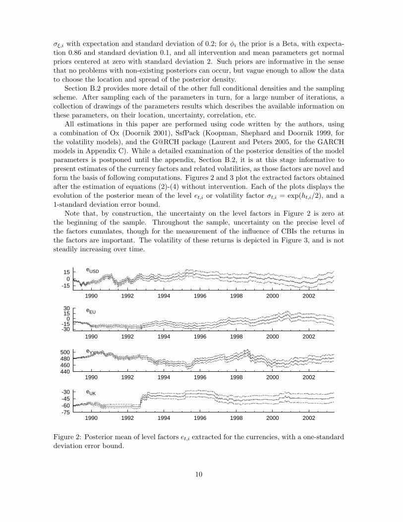
All estimations in this paper are performed using code written by the authors, usinga combination of Ox (Doornik 2001), SsfPack (Koopman, Shephard and Doornik 1999, forthe volatility models), and the G@RCH package (Laurent and Peters 2005, for the GARCHmodels in Appendix C). While a detailed examination of the posterior densities of the modelparameters is postponed until the appendix, Section B.2, it is at this stage informative topresent estimates of the currency factors and related volatilities, as those factors are novel andform the basis of following computations. Figures 2 and 3 plot the extracted factors obtainedafter the estimation of equations (2)-(4) without intervention. Each of the plots displays theevolution of the posterior mean of the level et,i or volatility factor σt,i = exp(ht,i/2), and a1-standard deviation error bound.

Note that, by construction, the uncertainty on the level factors in Figure 2 is zero atthe beginning of the sample. Throughout the sample, uncertainty on the precise level ofthe factors cumulates, though for the measurement of the influence of CBIs the returns inthe factors are important. The volatility of these returns is depicted in Figure 3, and is notsteadily increasing over time.

-15 0 15

1990 1992 1994 1996 1998 2000 2002

eUSD

-30-15 0 15 30

1990 1992 1994 1996 1998 2000 2002

eEU

440460480500

1990 1992 1994 1996 1998 2000 2002

eYY

-75-60-45-30

1990 1992 1994 1996 1998 2000 2002

eUK

Figure 2: Posterior mean of level factors et,i extracted for the currencies, with a one-standarddeviation error bound.

10

0.00.51.01.5

1990 1992 1994 1996 1998 2000 2002

σUSD

0.00.40.81.2

1990 1992 1994 1996 1998 2000 2002

σEU

0.00.71.42.1

1990 1992 1994 1996 1998 2000 2002

σYY

0.00.61.21.8

1990 1992 1994 1996 1998 2000 2002

σUK

Figure 3: Posterior mean of volatility factors σt,i = exp(ht,i/2) extracted for the currencies,with a one-standard deviation error bound.

Assessing the relevance of the factors

In order to illustrate the relevance of these extracted factors, we proceeded to some preliminaryanalysis. Bos and Shephard (2006) provide some economic interpretation of the unobservedcomponents, for both the level and the volatility of the currency components. For instance,they emphasise the impact of the EMS crisis on the volatility of each currency, stressing thedifferences across the various currencies. We invite the interested reader to refer to their paperfor such an interpretation. In a previous version of the paper, we have also how the extremevariations of the factors were related to important financial events. We found that for all thecurrencies, all highest variations of the factors are obviously related to well identified financialevents such as the EMS crisis, a major interest rate adjustment by the central banks and lastbut not least some direct interventions made by the monetary authorities. Interestingly, themajority of these particular events are country-specific or currency-specific events, i.e. shockspeculiar to a specific country or currency While informative, this type of analysis is onlysuggestive of some degree of relevance since one can argue that it is always possible to findan important financial event at each point of time. Therefore, we leave this piece of evidenceout of the current version of this paper.

A less arbitrary approach to assess the relevance of these factors is to compare relativeforecasting performances of the EGARCH and country factor SV (CFSV) models. FollowingAndersen and Bollerslev (1998), we do that through the analysis of the value of the coefficientof multiple correlation, or R2, in a Mincer-Zarnowitz regression approach (see Mincer andZarnowitz 1969). We nevertheless need a benchmark measure of volatility to assess thequality of these regressions. A traditional measure for the observed volatility in the literature

11

is the square of the returns or the absolute returns (Pagan and Schwert 1990). However,in a recent paper dealing with daily volatility, Andersen and Bollerslev (1998) have shownthat this measure is not fully relevant and have proposed an alternative measure. This newmeasure uses cumulated squared intradaily returns, also called realised volatility, which is amore precise measure of the daily volatility. Following these authors, we compute the dailyrealised volatility as:

RVt,ij(Q) =23∑

k=0

r2t,ij,Q−k, (8)

where rt,ij,Q denotes the intraday hourly return of the corresponding exchange rate peculiarto day t between quotation time Q − 1 and Q (by convention rt,ij,−Q = rt−1,ij,24−Q forQ = 1, 2, . . . , 23).

For a given quotation time Q (we drop the Q index for the sake of simplicity in thenotations), we project RVt,ij on a constant and the in-sample one-step-ahead forecast of ht,ij ,denoted Ft,ij|t−1, based on the EGARCH(1, 1) model of Nelson (1991) or on the CFSV modelwith unobserved components.9 More specifically the Mincer-Zarnowitz regression takes thefollowing form:

RVt,ij = a + bFt,ij|t−1 + ut, t = 1, . . . , T. (9)

Note that for the CFSV model, since the country components are assumed independent,

Ft,ij|t−1 ≡ exp(ht,i) + exp(ht,j). The forecasts of the factor standard deviations exp(ht,i) areextracted from a run of the particle filter (Pitt and Shephard 1999) at the posterior mode ofthe parameters of the model.

Recently, Andersen, Bollerslev and Meddahi (2005) have shown that the R2 of the Mincer-Zarnowitz regression (9) based on the realised volatility underestimates the true predictabilityof the competing models. To overcome this problem, they propose a simple methodology(based on the recent non-parametric asymptotic distributional results in Barndorff-Nielsen

and Shephard 2002) to obtain an adjusted R2, denoted R2, that takes into account the

measurement errors in the realised volatility.Table 1 reports the estimated parameters of the Mincer-Zarnowitz regressions (robust

standard errors are given between parentheses) as well as the R2’s and R2’s (between brackets)

of both the EGARCH(1, 1) model and the CFSV model (without CBIs dummies) estimatedon the three daily exchange rates vis-a-vis the USD, at quotation time Q = 16h00 GMT+1.

From Table 1, one hardly sees a difference between the two competing approaches in termsof bias. Indeed, irrespective of the specification, a and b are not significantly different from 0and 1 (at the usual 5% level), respectively for the YEN/USD and GBP/USD series. For theEUR/USD series, both models provide slightly biased estimates of the realised volatility sincethe β’s are significantly higher than 1. However, there is no doubt about the supremacy of the

unobserved components model in terms of predictability of volatility. Indeed, the R2’s and

R2’s are between 30% to almost 50% higher than the ones obtained from the EGARCH(1, 1)specification.10 Note that the same conclusion applies regardless we use a simple GARCH ora more sophisticated long-memory (E)GARCH model.

9We do not investigate the out-of-sample performance of these models since the models are only used toquantify the impact of interventions.

10Recall from statistics that the unadjusted R2 of a simple regression model is the square of the empiricalcorrelation between the endogenous variable and the regressor. For instance for the EUR/USD, R2

EGARCH =0.11 ≈ corr(RVt,ij , F

EGARCHt,ij|t−1 )2 = 0.332 whereas R2

CFSV = 0.22 ≈ corr(RVt,ij , FCFSVt,ij|t−1)

2 = 0.472.

12

Table 1: In-sample forecast comparisonMincer-Zarnowitz Regressions

Series EGARCH(1, 1) CFSV

a b R2[R2] a b R

2[R2]

EUR/USD -0.08 1.28 0.19 -0.10 1.34 0.38

(0.04) (0.10) [0.11] (0.05) (0.12) [0.22]YEN/USD -0.13 1.34 0.23 -0.17 1.43 0.40

(0.12) (0.26) [0.17] (0.13) (0.29) [0.30]GBP/USD -0.02 1.21 0.26 0.00 1.16 0.40

(0.03) (0.11) [0.19] (0.04) (0.13) [0.28]Note: Estimated parameters of the Mincer-Zarnowitz regression (9), either using the in-sample forecast of the standard deviation according to the EGARCH(1, 1) model (columns2-4) or using the CFSV model (columns 5-7). Robust standard errors are given between

parentheses. The adjusted R2’s (a la Andersen et al. 2005), denoted R2

, are reportedboldface in columns 4 and 7 while the unadjusted R2’s are reported below between brackets.

4 Data, estimation and results

4.1 Central bank intervention data

Our CBIs data capture daily official interventions (as disclosed by the central banks them-selves) conducted by the three major central banks over the period from January 1 1989 toMay 31 2003. The CBIs are used as daily signed dummies indicating the purchases or salesof foreign currencies relative to the USD. By convention, the intra-EMS intervention dummytakes a value of 1 for DEM sales, while the one for EUR/YEN interventions is 1 for sales ofthe Yen.

These data were obtained either through bilateral contacts with the central banks (Fedand European Central Bank) or through downloading the data from the website (Bank ofJapan). For these BoJ interventions, due to unavailability of official data before May 1991,the data capture the days of reported interventions for the first part of the sample. Note thatthe official interventions concerning the British Pound are not available, at least to externalresearchers; this currency is taken along only in the estimation in order to facilitate theestimation of the currency factors for levels and volatilities.

As usual in the literature, we distinguish between coordinated interventions (operationsconducted by the two involved central banks on the same markets, the same day and inthe same direction) from unilateral ones. The CBIs are captured by dummy variables asdone in most papers of the empirical literature and in a consistent way with the signallingchannel which is the underlying theoretical framework used to rationalise the impact of theseoperations on exchange rates.

We consider eight different types of interventions, indicated by the acronyms of the in-volved central banks and the exchange rate on which the intervention took place. The numberof intervention days broken down by type of operation and by currency market is reported inTable 2.

13

Table 2: Number of interventions days

YEN/USD EUR/USD EMS EUR/YEN

ECB-Fed - 58 - -BoJ-Fed 72 - - -

Fed 31 64 - -BoJ 227 - - 18ECB - 33 - -BB - - 33 -

Note: The figures report the number of interventions days on each market, over the sampleperiod of 1/1/1989-31/5/2003, by the indicated central banks. The intra-EMS interventionsare performed by the Bundesbank, before the ECB was founded in 1998.

4.2 Quotation time

While our analysis is conducted at the daily frequency, we pay particular attention to thechoice of the quotation time Q of the exchange rates St,ij . The importance of this choice stemsfrom the recent findings of the literature suggesting that the impact of CBIs on the momentsof exchange rate returns can be of short-run duration and mean-reverting (Dominguez 2003and 2004; Payne and Vitale 2003; Beine et al. 2004). As emphasised by Beine et al. (2004),such evidence stresses the importance of choosing an appropriate and separate quotation timeto study the impact of each type of operation. Appendix A discusses in detail the choice ofthe optimal quotation time relative to each type of operation.

Another approach is to conduct a pure intraday analysis on the impact of CBIs but thisis not feasible at present. First, the exact timings of the operations conducted by the threecentral banks studied here are not available. Secondly, conducting a pure intraday analysismay be cumbersome since intraday FX data are known to exhibit a complex seasonalitypattern. This intraday periodicity gives rise to a striking repetitive U-shape pattern in theautocorrelations of the absolute or squared returns, which are proxies for the volatility. Whiletheoretically feasible, extracting both the unobserved country specific volatilities and theirseasonality using the Bayesian methods developed by Bos and Shephard (2006) is obviouslybeyond the scope of the paper.

4.3 Results

Table 3 reports the estimates of the impact of CBIs on the currency factors. The columnsreport the posterior mean of the impact of CBIs on the currency components of the exchangerates (β and γ parameters), the standard deviation (s), the the 90% highest posterior densityregion (HPD(90%)), and an indicator for the significance of the parameter, (p). As in aBayesian setting there is no clear alternative to a classical p-value, we computed

pβ = 2 min [P (β < 0|Y ), 1 − P (β < 0|Y )]

with P (β < 0|Y ) the posterior probability of observing β < 0; likewise a pγ is computed.This statistic checks which part of the posterior density falls ‘on the other side of zero’, andcan be used as similarly to the classical p-value, though its theoretical background is ratherdifferent. For simplicity, we refer to this statistic in subsequent sections directly as a p-value,without indicating its Bayesian background.

14

The upper panel of the table (labelled ‘Mean equation’) reports the findings relative tothe mean (first moments of the country factors) while the lower panel (labelled ‘Varianceequation’) provides the results relative to the volatility side (second moment of the countryfactor increments).

For the sake of brevity, we only report the estimates of the impact of each type of operation.It should be nevertheless clear that each estimate comes from the estimation of the full model,i.e. the one admitting a specification in which all components of Wt,i are included both inthe mean and variance equations. The model is estimated using a quotation time Q for St,ij

corresponding to the likelihood of the occurrence of the investigated operation. This timing isreported in column 3. For instance, the estimates of the impact of coordinated interventionsof the Fed and the ECB are reported from the estimation of the models using St,ij observedat Q = 15h GMT+1, as this is the quotation timing around which the interventions are mostlikely to have taken place. The choice of the optimal quotation time is motivated in AppendixA.

4.3.1 Mean results

If one defines an effective operation as the one moving the exchange rate in the desireddirection, i.e. net purchases of dollars leading to an appreciation of the dollar, an effi-cient operation implies positive coefficients on the non-US (Euro or Yen) component (i.e.βEUR > 0, βYEN > 0) and negative coefficients on the US component (i.e. βUS < 0).11 Animportant exception concerns the impact of the so-called auxiliary interventions. While itwould be impossible to interpret the coefficient obtained for these interventions (BB withinthe EMS, and the BoJ on the EUR/YEN market) in a EGARCH specification, efficiency inthe factor approach implies a positive coefficient on the Euro component associated to EMSinterventions, a negative coefficient on the Euro component associated to interventions on theEUR/YEN and a positive coefficient on the YEN component associated to interventions onthe EUR/YEN.

Consistent with the findings obtained in the EGARCH approach (see Appendix C) inparticular and by the empirical literature in general, our factor approach also points to pooreffectiveness of interventions. Nevertheless, we do not find any evidence of counterproductiveimpact in terms of the currencies. An interesting contribution of our factor approach lies inthe estimated impact of the intra-EMS interventions conducted by the Bundesbank. Lookingat the impact in terms of the Euro component, the results point to some (weakly) efficientoperations of the Bundesbank since in general DEM sales tended to lower the value of theGerman currency. The same holds for the sales of YEN against the Euro carried out by theBoJ which tended to appreciate the European currency. These results illustrate that auxiliaryinterventions are easier to interpret in a currency factor model. They show that they turn outto be important control variables to be taken into account in an econometric analysis aimedat capturing the effect of CBIs.

11As discussed by several authors like Fatum (2002), such a definition of efficiency might be very restrictivein the sense that there is no guarantee that it matches the objective(s) of the central bank. Such a definitionnevertheless conveys the advantage of simplicity and delivers a testable proposition.

15

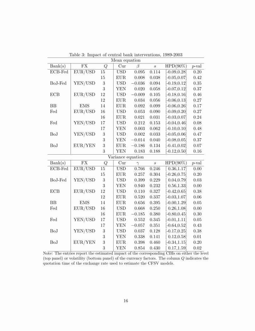
Table 3: Impact of central bank interventions, 1989-2003Mean equation

Bank(s) FX Q Cur β s HPD(90%) p-val

ECB-Fed EUR/USD 15 USD 0.095 0.114 [-0.09,0.28] 0.2015 EUR 0.008 0.038 [-0.05,0.07] 0.42

BoJ-Fed YEN/USD 3 USD −0.036 0.094 [-0.19,0.12] 0.353 YEN 0.020 0.058 [-0.07,0.12] 0.37

ECB EUR/USD 12 USD −0.009 0.105 [-0.18,0.16] 0.4612 EUR 0.034 0.056 [-0.06,0.13] 0.27

BB EMS 14 EUR 0.092 0.099 [-0.06,0.26] 0.17Fed EUR/USD 16 USD 0.053 0.090 [-0.09,0.20] 0.27

16 EUR 0.021 0.031 [-0.03,0.07] 0.24Fed YEN/USD 17 USD 0.212 0.153 [-0.04,0.46] 0.08

17 YEN 0.003 0.062 [-0.10,0.10] 0.48BoJ YEN/USD 3 USD 0.002 0.033 [-0.05,0.06] 0.47

3 YEN −0.014 0.040 [-0.08,0.05] 0.37BoJ EUR/YEN 3 EUR −0.186 0.134 [-0.41,0.02] 0.07

3 YEN 0.183 0.188 [-0.12,0.50] 0.16

Variance equation

Bank(s) FX Q Cur γ s HPD(90%) p-val

ECB-Fed EUR/USD 15 USD 0.766 0.246 [ 0.36,1.17] 0.0015 EUR 0.257 0.304 [-0.26,0.75] 0.20

BoJ-Fed YEN/USD 3 USD 0.399 0.229 [ 0.04,0.79] 0.033 YEN 0.940 0.232 [ 0.56,1.33] 0.00

ECB EUR/USD 12 USD 0.110 0.327 [-0.42,0.65] 0.3812 EUR 0.520 0.337 [-0.03,1.07] 0.06

BB EMS 14 EUR 0.656 0.395 [-0.00,1.29] 0.05Fed EUR/USD 16 USD 0.668 0.250 [ 0.26,1.08] 0.00

16 EUR −0.185 0.380 [-0.80,0.45] 0.30Fed YEN/USD 17 USD 0.552 0.345 [-0.01,1.11] 0.05

17 YEN −0.057 0.351 [-0.64,0.52] 0.43BoJ YEN/USD 3 USD 0.037 0.128 [-0.17,0.25] 0.38

3 YEN 0.338 0.141 [ 0.12,0.58] 0.01BoJ EUR/YEN 3 EUR 0.398 0.460 [-0.34,1.15] 0.20

3 YEN 0.854 0.430 [ 0.17,1.59] 0.02Note: The entries report the estimated impact of the corresponding CBIs on either the level(top panel) or volatility (bottom panel) of the currency factors. The column Q indicates thequotation time of the exchange rate used to estimate the CFSV models.

16

4.3.2 Volatility results

With respect to the volatility side, the factor approach adopted in this paper sheds someinteresting light on the impact of these interventions. The distinction between currencycomponents allows to identify significant impacts which are not captured in the classicalapproach in terms of exchange rates. The discrepancy in terms of findings between the twoapproaches is partly due to the fact that the impact in terms of exchange rates is a non-linearcombination of the impacts in terms of currency components.

First, the CBIs are not found to affect the volatility of the USD more than the volatilityof the other currencies involved in the FX operation. In this respect, the results are notsupportive of the existence of any USD-bias in the investigation of CBIs and suggest a negativeanswer to Question 2 concerning the existence of a specific dollar effect.

Second, the results of the factor approach allow to document interesting asymmetric effectsof CBIs in terms of volatility. The results in Table 3 suggest that unilateral interventions tendto exert highly asymmetric effects in terms of the volatility of the currencies, judging fromthe location of the 90% HPD region and the p-value. It is found that unilateral CBIs tendto impact the volatility of the currency of the central bank conducting the intervention.For instance, a unilateral intervention conducted by the Fed tends to primarily impact theuncertainty of the US currency (see the coefficients of the Fed:EUR/USD and Fed:YEN/USD).Strikingly, the same result holds for the BoJ on the YEN/USD as well for the ECB onEUR/USD. These results question the usual conclusion of the empirical literature emphasisingthe absence of any impact of unilateral interventions. They suggest that operations of thistype not only fail to deliver the desired effect in terms of level of the currency but alsoinvolve some significant costs in terms of uncertainty.12 Interestingly, this contrasts withthe impact associated to concerted operations. The coordinated interventions between theFed and the BoJ are indeed found to affect the volatility of both currency components.Such evidence is less obvious for the coordinated interventions between the Fed and theECB, with about 10% of the posterior probability mass indicating negative values of γ(ECB-Fed:EUR). On the whole, these results are also clearly supportive of an operating signallingchannel for the FOREX interventions in the sense that the operations mostly affect theexpectations of agents regarding the currency of the central bank present in the marketand not the other currency component. Our results suggest that depending on the type ofoperation, interventions induce different impacts on the currency market, at least in terms ofvolatility. The existence of general asymmetric effects of concerted and unilateral operationsis broadly speaking consistent with previous evidence.13 Hence, the answer to Question 1, onthe evidence of asymmetric effects between unilateral and concerted operations, is obviouslyaffirmative.

Another interesting insight concerns the impact of auxiliary interventions. Unlike the ap-proach in terms of exchange rates, the decomposition in currency factors succeeds in capturingvolatility effects of these interventions. The rationale for this result might be the following.Referring to the signalling channel which has by far received the most important empiricalsupport, there is no theoretical reason why we should expect some intra-EMS interventions or

12Once more, we implicitly adopt here the usual view that central banks tend to dislike bursts of volatility oftheir currencies. This view has nevertheless been scarcely questioned by a couple of authors (e.g. Hung 1997).

13See for instance Beine, Laurent and Lecourt (2003) showing that depending on the level of volatility, theconcerted interventions might deliver positive or negative impact. Such an effect does not hold for unilateraloperations.

17

interventions on the DEM/YEN market to impact the volatility of the USD. As a result, thevariation of the exchange rate expressed in USD is likely to be smoothed, in comparison withthe variation of the EUR or YEN components. In contrast, the identification of the currencycomponent allows to abstract from this drawback and permits a clear identification of theincrease of the volatility. These results imply that auxiliary interventions tend to have someindirect impact on the exchange rate and could be considered as relevant control variables infuture investigations of the impact of CBIs. In this sense, they lead to a positive answer toQuestion 3.

5 Conclusion

In this paper, we assess the impact of foreign exchange interventions carried out by the G-3central banks over the recent period. Unlike the traditional approaches in terms of exchangerates, we propose to investigate the impact of these operations on the first two moments ofthe currency components of these exchange rates. The identification of these componentsis carried out through the estimation of a recent currency factor stochastic volatility modelproposed by Bos and Shephard (2006) augmented by explanatory variables both in the meanand the volatility parts. Through the analysis of the effects of the central bank interventions,our paper provides a first attempt to capture asymmetric effects of financial news in theforeign exchange markets in terms of currencies.

Our results provide new insights on the impact of these interventions. First, they confirmthat in general, central bank operations do not succeed in moving the exchange rate in thedesired direction and tend to lead to more uncertainty. Nevertheless, our results in termsof currency dynamics are not, in contrast with some previous empirical studies based onmore traditional approaches, supportive of perverse effects associated to these operations.Second, our results do not support the existence of some USD bias in the sense that the UScurrency would be impacted more by direct purchases or sales performed by the major centralbanks. Third and importantly, while the traditional approaches do not identify clear effectsin terms of exchange rate volatility, we find that unilateral interventions obviously tend toprimarily raise the volatility of the currency of the central bank involved in these operations.This contrasts with the effect associated with concerted operations and might be consideredas some additional evidence in favour of the signalling channel hypothesis for the effect ofinterventions. Finally, our approach allows to capture in a more rational way the impact ofoperations carried out by the central banks on other, possibly indirectly related, markets.

This paper can be extended to a full intra-day analysis. Such an analysis however shouldovercome the fact that exact timings of official interventions are not available. This couldbe done by relying on the timings extracted from the newswire reports as proposed byDominguez (2004). Another hurdle concerns the application of the estimation techniquesto high-frequency data as well as the way to account for intra-daily seasonality patterns andfor the occurrence of micro-structure noise induced by the high frequency. These extensionsare left for future research.

18

A Timing of CBIs

As explained in Section 4.2, the choice of the quotation time of the exchange rate is of primaryimportance for assessing the impact of CBIs on the dynamics of exchange rates and currencycomponents. In this appendix, we discuss for each type of operation the choice of the optimalquotation time, i.e. the quotation time necessary to capture, the potential impact of theseoperations. Basically, we can rely on a set of elements which, together, suggest a likely timerange:

• The opening hours of the local markets. As documented by Dominguez (1998, 2003),most central banks tend to operate on their own local markets, providing orders to thedomestic commercial banks;

• The need to coordinate with another central bank, for concerted operations;

• The empirical distribution of the timings of reported interventions for each central bank(Dominguez 2003).

The empirical distributions involve the timing of the interventions perceived by the FX tradersusing Reuters’ newswire reports. They nevertheless ignore the secret, unreported interven-tions, which according to Dominguez (2003) may account for up to 25% of the Fed inter-ventions over the 1989-1995 period. They also do not account for the possible lags betweenthe effective operations and the trader reports. Recent results obtained by Payne and Vitale(2003) show that exchange rates react up to 45 minutes ahead of Reuters’ intervention re-ports on operations of the Fed. Importantly, the lengths of these lags may be variable as thereporting depends on the dealers’ willingness to release the information.

The moments of these distributions, together with information on the opening hours ofthe local markets of the intervening banks, nevertheless provide useful insight in the possibletiming of the operations.

A.1 Coordinated interventions on the EUR/USD

Following the discussions in Dominguez (1998, 2003) as well as the evidence of Beine et al.(2004) with respect to impact of CBIs on volatility, we assume that the coordinated inter-ventions of the Fed and the ECB take place during the overlap period (ranging between 13hand 17h GMT+1). Such a choice is consistent with the distribution over time provided byDominguez (2003) using Reuters’ reports. We therefore pick up the middle of the time rangefor the exchange rate quotation, i.e. 15h GMT+1. This choice is consistent with the evidenceprovided by Beine et al. (2004).

A.2 Coordinated interventions on the YEN/USD

Unlike coordinated interventions between the ECB and the Fed, there is no overlap periodbetween the Japanese and the US market. Therefore, assuming that most interventionsare carried out by central banks on their own local markets (see Dominguez 2003, on thisparticular point), a coordinated intervention on this market takes the form of an interventionof the BoJ followed by an intervention of the Fed. An initial BoJ intervention will thereforeinduce some reaction of the markets during Japanese trading time. We therefore investigatethe impact using the middle of the time range for the exchange rate quotation, i.e. at 3hGMT+1.

19

A.3 Unilateral interventions of the ECB on the EUR/USD

When carrying out a unilateral operation, the ECB (or Bundesbank) does not need to takeadvantage of the simultaneous opening of the US and the European market. Therefore, theoperation can take place either before or after the opening of the US market (13h GMT+1).Such a procedure is consistent with the evidence provided by Dominguez (2003) documentingan average time of occurrence of ECB operations around 12h30 GMT+1. We therefore usethe quotation at 12h GMT+1.

A.4 Intra-EMS interventions of the BB affecting the EUR/USD

All EMS interventions are coordinated interventions in the sense that they involve the sameoperation on the part of the BB and other European central banks. Notice that we do not havethe counterpart EMS currency against which the German Mark was traded, and therefore donot know which second European central bank was involved in these operations. Given thefact that these operations can occur all over the day, we choose 14h GMT+1 as our exchangerate quotation.

A.5 Unilateral interventions of the Fed on the EUR/USD and the YEN/USD

The evidence provided by Dominguez (2003) documents an average time of occurrence of theFed operations around 15h57 GMT+1. It should be stressed that the reported figures mixinterventions on the YEN/USD and the EUR/USD market. For the interventions on theEUR/USD, the Fed can nevertheless take advantage of the overlap period with the Europeanmarket to increase the visibility of its interventions. Therefore, we choose quotation 16hGMT+1. For the unilateral interventions of the Fed on the YEN/USD market, we use thequotation 17h GMT+1 since there is no overlap with Asian markets.

A.6 Unilateral interventions of the BoJ on the YEN/USD and the EU/YEN

Given the stylised fact that most central banks use a network of domestic commercial banks tocarry out their interventions, it might be inferred that the vast majority of BoJ interventionsare carried out between 0h and 7h GMT+1. This is confirmed by the evidence given byDominguez (2003), with an average BoJ intervention time around Tokyo lunchtime, with amean at 4h56 GMT+1. Like for the coordinated interventions, we choose 3h GMT+1 as ourquotation time.

20

B Posterior sampling

B.1 Statistical background

The currency factor-stochastic volatility model presented in Section 3 is built up from unob-served components et,i for the level and ht,i for the volatility of the exchange rates. For easeof reference, the model was written as

st,ij = et,i − et,j , i, j = 0, . . . , n, (1)

et+1,i = βt,i + et,i + ǫt,i, ǫt,i ∼ N (0, exp(ht,i)), (2, 3)

ht+1,i − γt+1,i = φi(ht,i − γt,i) + ξt,i, ξt,i ∼ N (0, σ2ξ,i) ≡ N (0, (1 − φi)

2σ2h,i), (4, 5)

with βt,i and γt,i including the regression effects of the interventions, and t = 0, . . . , T , andσ2

h = σ2ξ/(1 − φ2) the long-run variance of the SV equation.

The country factors are initialised at e0,0 ≡ 0 for the numeraire country, and all otherfactors e0,i ≡ s0,i0, i 6= 0 at the respective log-exchange rate. The volatility sequences areinitialised diffusely, with h0,j ∼ N (γ0,j , κ), κ → ∞, j = 0, . . . , n. As long as there are at least3 countries involved, this model is identified with these initialisations.

The relation between (log-) exchange rates st,ij and the respective volatilities ht,i, ht,j isclearly non-linear. In such a case, convenient classical estimation methods are not available.Therefore, we apply a Bayesian estimation procedure to this model (see Doucet, de Freitasand Gordon 2001, for an introduction to Markov chain Monte Carlo sampling techniques),using a sampling scheme for stochastic volatility models which was developed originally inpapers like Harvey et al. (1994), Jacquier et al. (1994) and Kim et al. (1998), and furtherrefined for the case of multiple SV sequences on longer time horizons by Bos and Shephard(2006).

In this last paper, a Bayesian sampling procedure is proposed for models with sto-chastic volatility and a conditionally Gaussian State Space form (GSSF-SV). The variantof the algorithm applied here samples from the augmented parameter space consisting ofθ = (σh, φ, γ, β) and unobserved components e = {et,i, t = 0, . . . , T, i = 0, . . . , n} andh = {ht,i, t = 0, . . . , T, i = 0, n}. It applies a transformation from the volatility sequence

hi to the standardised disturbances ut,i ≡ ξt,i/(√

1 − φ2i σh,i) = f−1(h, σh, φ, γ) of the volatil-

ity processes, for sampling the parameters φ, σh|u, e, as this improves the convergence of thesampling algorithm greatly.

The sampling procedure follows a Gibbs sampling scheme, where the parameters aresampled in blocks, conditional on all other parameters of the model. This sampling density,the full conditional posterior density, is constructed as a combination of the likelihood ofthe model and the prior density of the parameters; based on earlier experience with similarmodels the priors as specified in Table 4 are chosen. These priors are chosen to be only mildlyinformative, such as to assure existence of all conditional posterior densities, but allow theinformation in the likelihood to determine the location and shape of the posterior density.

With these preliminaries settled, the final algorithm applies the following steps:

1. Initialise h, θ;

2. Sample from e|s,h, θ using the generic GSSF simulation smoother (Fruhwirth-Schnatter1994, Carter and Kohn 1994, De Jong and Shephard 1995, Durbin and Koopman 2002);

21

Table 4: Prior specificationsParameter Density Expectation Standard deviation

σh,i Inverted Gamma 0.5 0.2φi Beta 0.86 0.1γ, β Normal 0 2

3. Sample from h|e, s, θ, using the method in Kim et al. (1998). Effectively, sampling isdone successively from ht|ht−1, ht+1, θ, s, for t = 1, . . . , T ;

4. Update draw from θ|e,h by

(a) Sampling from β|e,h from its Gaussian conditional density;

(b) Likewise, sample γ|h, φ, σh, also from its Gaussian conditional density;

(c) Construct u = f(h, θ), sample φ, σh|u, γ using a random walk Metropolis-Hastingsstep, separately for the parameters of each currency, and reconstruct h from u andθ;

5. Repeat from 2.

From Bos and Shephard (2006) stems the idea to sample φ, σh|u instead of conditioningon h, and to do so per currency. As the persistence of volatility in the U.S. is purport-edly not related to the persistence in the Euro area, the parameters can be supposed largelyindependent. Therefore, sampling can be done separately without introducing extra corre-lation in the chain of draws from the parameter space. Not used is the option to samplealso the intervention parameters to the volatility process, the γ’s, conditional on u, as theconditional density γ|u, φ, σh is a, computationally very demanding, convolution of GumbelExtreme Value densities. Instead of lowering the value of the correlation using this option, itwas found more advantageous to use a larger sample.

This sampling scheme delivers draws from the posterior density of the parameters in θand of the unobserved components e,h. Note that all the sampled values are based onall exchange rates, over the full time period. In terms of the state space model, the samplescorrespond to ‘smoothed’ estimates, instead of filtered estimates. In case full filtered estimatesare requested, as in the Mincer-Zarnowitz regressions of Table 1, a particle filter was used(Pitt and Shephard 1999).

B.2 Resulting posterior density

Using the method exposed in Section B.1, a collection of the parameters σh, φ, γ, β (andfactors e and h) is sampled from the posterior density. The sample size was 100,000, after aburn-in period of 10,000 iterations.

While the main interest lies in the sampled factors, the model parameters σh, φ, γ, β playtheir own role in modelling persistence of the stochastic volatility, and the size of the influenceof each type of the CBIs.

Table 5 displays the posterior mean, the standard deviation, the 90% highest posteriordensity region, and the inefficiency measure as highlighted in Shephard and Pitt (1997). Theinefficiency measure indicates the amount of correlation in the chain, comparing the variationof the parameter to a measure of variation adapted for the autocorrelation at a window of

22

the size of 2,000 lags. A theoretical value of 1 would indicate a fully efficient sample withindependent drawings, whereas high values are a sign of higher correlation in the chain andhence lower efficiency of the sampling method.

Table 5: Posterior statistics for the currency factor SV modelParameter Factor Mean Std. dev HPD(90%) Inefficiency

φ USD 0.978 0.007 [0.97, 0.99] 1598.97EUR 0.975 0.007 [0.96, 0.99] 1586.08YEN 0.960 0.011 [0.94, 0.98] 773.15GBP 0.968 0.010 [0.95, 0.98] 1548.18

γ0 USD −1.796 0.132 [−2.01, −1.58] 36.41EUR −2.187 0.139 [−2.41, −1.96] 21.42YEN −1.286 0.107 [−1.46, −1.11] 41.52GBP −3.086 0.215 [−3.44, −2.73] 111.18

σh USD 0.771 0.072 [0.66, 0.88] 894.93EUR 0.867 0.081 [0.74, 0.99] 1120.59YEN 0.847 0.065 [0.74, 0.95] 318.39GBP 1.415 0.130 [1.20, 1.62] 532.93

Note: The table reports the posterior mean, standard deviation, 90% highest posteriordensity region, and the inefficiency measure (Shephard and Pitt 1997), for the parametersgoverning the autocorrelation, overall level of the stochastic volatility and the long-runvariance of the volatility.

0.94 0.96 0.98

φUS

PosteriorPrior

0.94 0.96 0.98

φEU

0.92 0.94 0.96 0.98

φYY

0.92 0.94 0.96 0.98

φUK

-2.4 -2 -1.6 -1.2

γUS

-2.8 -2.4 -2 -1.6

γEU

-1.6 -1.2 -0.8

γYY

-4 -3.5 -3 -2.5 -2

γUK

0.6 0.8 1 1.2

σh, US

0.6 0.8 1 1.2

σh, EU

0.6 0.8 1 1.2

σh, YY

1 1.25 1.5 1.75 2

σh, UK

Figure 4: Posterior distribution of parameters of the currency factor SV model, withoutinterventions, at quotation time 16h GMT+1

The results of the table suggest that the posteriors of σh and φ are quite concentrated, and

23

also the posteriors of the γ0 parameters governing the overall level of volatility are estimatedclearly away from the prior mean (see Table 4 for the prior specifications), hence the data isinformative on these parameters. This effect is more easily seen in Figure 4, where the priorand posterior densities are drawn together.

Though the data is informative on the parameters, the posterior sample correlation re-mains high, even after applying the some of the methods of Bos and Shephard (2006).14

Especially for parameters φ and σh, correlation is still rather strong, but from Figure 4 itis seen that the posterior densities are smooth, a clear indication of convergence. For theintervention parameters, β gives inefficiency statistics below 40, and thus is not problematicat all, but γ is harder to estimate. It’s inefficiencies in the final sample range between 200and 700. The sample size of 100,000 however was large enough to ensure convergence, andthe resulting sample could be used without problem for the analysis in previous sections.

C EGARCH results

For the sake of comparison, we complement our analysis in terms of country factors bya traditional GARCH analysis aimed at capturing the impact of interventions on the firsttwo moments of the exchange rate returns. As surveyed by Humpage (2003), this type ofapproach has been extensively used in the empirical literature and might be considered as auseful benchmark to assess the contribution of our analysis.

To this aim, we rely on a standard EGARCH(1, 1) specification (Nelson 1991) with CBIsintroduced both in the conditional mean and variance equations: Defining the exchange returnrt,ij as rt,ij = st,ij − st−1,ij , the EGARCH(1, 1) model is specified as follows

rt,ij = β†t,ij + ǫt,ij , (10)

ǫt,ij ≡ exp(ht,ij/2)zt,ij , zt,ij ∼ N (0, 1),

ht,ij = γ†t,ij + ϑ†

1,ijzt−1,ij + ϑ†2,ij [|zt−1,ij | − E(|zt,ij |)] + δ1,ijht−1,ij , (11)

where ϑ†1,ij , ϑ

†2,ij and δ†

1,ij are parameters governing the evolution of the GARCH process.The CBIs are introduced both in the conditional mean and variance equations. They follow asimilar setup as in the CFSV model (see equations (6) and (7)). The interventions influenceequations (10)–(11) through

β†t,ij = β†

0,ij + Wt,ijβ†1,ij , (12)

γ†t,ij = γ†

0,ij + |Wt,ij |γ†1,ij , (13)

where Wt,ij is a vector of indicators identical to the one used in equations (6) and (7).

β†ij = (β†

0,ij , β†1,ij) and γ†

ij = (γ†0,ij , γ

†1,ij) are the corresponding vectors of parameters. Unlike

the CFSV model, these two vectors of parameters capture the effect of CBIs on the dynamicsof the exchange rate returns or the EUR, YEN and GBP vis-a-vis the USD rather than in

14Apart from measures taken here, also the parameters β could be taken up into the state along withthe currency levels e, such that they are sampled within the simulation smoother; parameters γ could besampled conditional on disturbances u instead of conditioning on the volatility process h. Both methods lowerthe correlation in the chain, but at the cost of a large increase in computation time given the number ofinterventions applied. It was not deemed necessary for this analysis to use these two additional steps.

24

terms of the country specific components. The estimation of the model is done by quasi-maximum likelihood using the G@RCH 4.0 package (see Laurent and Peters 2005).

It should be first emphasised that in general, the results obtained in the empirical liter-ature using GARCH models are to a certain extent sample-specific (Humpage 2003). Thispartly reflects that intervention policies change over time. This explains why our EGARCHresults are representative of this literature only to some degree and that there exists somediscrepancies with previous studies. The choice of the ‘optimal’ quotation time, the use of aspecific GARCH model and the type of interventions might also explain these discrepancies.15

Table 6: EGARCH estimates of central bank interventions, 1989-2003Mean equation

Bank(s) FX Q β†1 s p

ECB-Fed EUR/USD 15 -0.138 0.161 0.20BoJ-Fed YEN/USD 3 -0.311 0.122 0.01ECB EUR/USD 12 -0.277 0.184 0.07BB EMS 14 0.009 0.136 0.49Fed EUR/USD 17 -0.095 0.067 0.08Fed YEN/USD 17 -0.192 0.129 0.07BoJ YEN/USD 3 -0.279 0.060 0.00BoJ EUR/YEN 3 0.275 0.130 0.02

Variance equation

Bank(s) FX Q γ†1 s p

ECB-Fed EUR/USD 15 0.918 0.299 0.00BoJ-Fed YEN/USD 3 0.444 0.056 0.00ECB EUR/USD 12 0.098 0.122 0.40BB EMS 14 0.166 0.078 0.02Fed EUR/USD 17 -0.040 0.043 0.17Fed YEN/USD 17 -0.170 0.122 0.09BoJ YEN/USD 3 0.051 0.037 0.09BoJ EUR/YEN 3 -0.220 0.124 0.04

Note: The entries report the estimated impact of the corresponding CBIs (see columns 1and 2), based on the EGARCH model. The column Q indicates the quotation time of theexchange rate used to estimate the EGARCH models. The columns marked by s and preport the robust standard errors and the p-value for a one-sided test of significance of theparameters.

The EGARCH results are reported in Table 6. Basically, these results might be sum-marised as follows. First, there is some very weak evidence that CBIs succeed in movingthe exchange rate in the desired direction. This points to a low degree of effectiveness ofthis policy instruments. Second, there is more evidence that CBIs tend to affect exchangerate volatility in a systematic way. In general, interventions lead to a subsequent increasein volatility, which is fully in line with what is found in many other papers. Finally, thereis some clear evidence that concerted operations affect much more exchange rate volatilitycompared to unilateral operations. This illustrates the so-called asymmetric effect betweenthese two types of intervention.

15For instance, using reported interventions of the BoJ before 1991, Beine et al. (2002) find some significantimpact of the coordinated interventions on the YEN/USD over the 1985-1995 period.

25

References

Andersen, T. G. and Bollerslev, T. (1998), ‘Answering the skeptics: Yes, standard volatilitymodels do provide accurate forecasts’, International Economic Review 39, 885–905.

Andersen, T. G., Bollerslev, T. and Meddahi, N. (2005), ‘Correcting the errors: Volatilityforecast evaluation using high-frequency data and realized volatilities’, Econometrica

73, 279–296.

Barndorff-Nielsen, O. and Shephard, N. (2002), ‘Econometric analysis of realized volatilityand its use in estimating stochastic volatility models’, Journal of the Royal Statistical

Society, B 63, 167–207.

Beine, M. (2004), ‘Conditional covariances and direct central bank interventions in the foreignexchange markets’, Journal of Banking & Finance 28, 1385–1411.

Beine, M., Benassy-Quere, A. and Lecourt, C. (2002), ‘Central bank interventions and foreignexchange rates: New evidence from FIGARCH estimations’, Journal of International

Money and Finance 21, 115–144.

Beine, M., Laurent, S. and Lecourt, C. (2003), ‘Central bank interventions and exchangerate volatility: Evidence from a switching regime analysis’, European Economic Review

47(5), 891–911.

Beine, M., Laurent, S. and Palm, F. C. (2004), Central Bank forex interventions assessedusing realized moments, Core Discussion Paper 2004/1, UCL, Louvain-la-Neuve.

Beine, M. and Lecourt, C. (2004), ‘Secret and reported interventions in the fx market’, Finance

Research Letters 1(4), 215–225.

Bhattacharya, U. and Weller, P. (1997), ‘The advantage to hiding one’s hand: Speculationand central bank inyervention in the foreign exchange market’, Journal of Monetary

Economics 39, 251–277.

Bonser-Neal, C. and Tanner, G. (1996), ‘Central bank intervention and the volatility of foreignexchange rates: Evidence from the options market’, Journal of International Money and

Finance 15(6), 853–878.

Bos, C. S., Mahieu, R. J. and Van Dijk, H. K. (2000), ‘Daily exchange rate behaviour andhedging of currency risk’, Journal of Applied Econometrics 15, 671–696.

Bos, C. S. and Shephard, N. (2006), ‘Inference for adaptive time series models: Stochasticvolatility and conditionally Gaussian state space form’, Econometric Reviews . Forth-coming.

Carnero, M. A., Pena, D. and Ruiz, E. (2001), Is stochastic volatility more flexible thanGARCH?, Statistics and Econometrics Series WP 01-08, Universidad Carlos III deMadrid.

Carter, C. K. and Kohn, R. (1994), ‘On Gibbs sampling for state space models’, Biometrika

81, 541–553.

26

De Jong, P. and Shephard, N. (1995), ‘The simulation smoother for time series models’,Biometrika 82, 339–350.

Detken, C. and Hartman, P. (2000), The euro and international capital markets. ECB Workingpaper nr. 19.

Dominguez, K. (2003), ‘The market microstructure of central bank intervention’, Journal of

International Economics 59, 25–45.

Dominguez, K. M. (1998), ‘Central bank intervention and exchange rate volatility’, Journal

of International Money and Finance 17, 161–190.

Dominguez, K. M. (2004), When do central bank interventions influence intra-daily and long-term exchange rate movements. Forthcoming in Journal of International Money and

Finance.

Doornik, J. A. (2001), Object-Oriented Matrix Programming using Ox, Timberlake Consul-tants Ltd, London. See http://www.doornik.com/.

Doucet, A., de Freitas, N. and Gordon, N. (2001), Sequential Monte Carlo Methods in Prac-

tice, Springer-Verlag, New York.

Durbin, J. and Koopman, S. J. (2001), Time Series Analysis by State Space Methods, OxfordUniversity Press, Oxford.

Durbin, J. and Koopman, S. J. (2002), ‘A simple and efficient simulation smoother for statespace time series analysis’, Biometrika 89, 603–615.

Evans, M. D. D. and Lyons, R. K. (2005), Are different-currency assets imperfect substitutes?,in P. De Grauwe, ed., ‘Exchange Rate Economics: Where Do We Stand?’, MIT Press,pp. 1–38.

Fatum, R. (2002), ‘Post-plaza intervention in the DEM/USD exchange rate’, The Canadian

Journal of Economics 35, 556–567.

Frenkel, J. (1976), ‘A monetary approach of the exchange rate: Doctrinal aspects and empir-ical evidence’, Scandinavian Journal of Economics 78, 200–224.

Fruhwirth-Schnatter, S. (1994), ‘Data augmentation and dynamic linear models’, Journal of

Time Series Analysis 15, 183–202.

Harvey, A. C. (1989), Forecasting, Structural Time Series Models and the Kalman Filter,Cambridge University Press, Cambridge.

Harvey, A. C., Ruiz, E. and Shephard, N. (1994), ‘Multivariate stochastic variance models’,Review of Economic Studies 61, 247–264.

Humpage, O. F. (2003), Government intervention in the foreign exchange market, Workingpaper 315, Federal Reserve Bank of Cleveland.

Hung, J. (1997), ‘Intervention strategies and exchange rate volatility: a noise trading per-spective’, Journal of International Money and Finance 16, 779–793.

27

Jacquier, E., Polson, N. G. and Rossi, P. E. (1994), ‘Bayesian analysis of stochastic volatilitymodels’, Journal of Business & Economic Statistics 12, 371–417.

Kim, S., Shephard, N. and Chib, S. (1998), ‘Stochastic volatility: Likelihood inference andcomparison with ARCH models’, Review of Economic Studies 64, 361–393.

Koopman, S. J., Shephard, N. and Doornik, J. A. (1999), ‘Statistical algorithms for modelsin state space using SsfPack 2.2’, Econometrics Journal 2, 107–160.

Laurent, S. and Peters, J.-P. (2005), G@RCH 4.0, Estimating and Forecasting ARCH Models,Timberlake Consultants.

Mahieu, R. J. and Schotman, P. C. (1994), ‘Neglected common factors in exchange ratevolatility’, Journal of Empirical Finance 1, 279–311.

Mincer, J. and Zarnowitz, V. (1969), The Evaluation of Economic Forecasts, Economic Fore-casts and Expectations, in J. Mincer, New York: National Bureau of Economic Research.

Mussa, M. (1981), The role of official intervention. Group of Thirty Occasional Papers no. 6,Group of Thirty, New York.

Nelson, D. B. (1991), ‘Conditional heteroskedasticity in asset returns: A new approach’,Econometrica 59, 349–370.

Pagan, A. and Schwert, G. (1990), ‘Alternative models for conditional stock volatility’, Jour-

nal of Econometrics 45, 267–290.

Payne, R. and Vitale, P. (2003), ‘A transaction level study of the effects of central bankintervention on exchange rates’, Journal of International Economics 61(2), 331–352.

Pitt, M. K. and Shephard, N. (1999), ‘Filtering via simulation: Auxiliary particle filters’,Journal of the American Statistical Association 94, 590–599.

Sarno, L. and Taylor, M. P. (2001), ‘Official intervention in the foreign exchange market: isit effective and, if so, how does it work?’, Journal of Economic Literature 39, 839–868.

Shephard, N. and Pitt, M. K. (1997), ‘Likelihood analysis of non-gaussian measurement timeseries’, Biometrika 84, 653–667.

Tims, B. and Mahieu, R. J. (2003), A range-based multivariate model for exchange ratevolatility, ERIM Report Series ERS-2003-022-F&A, ERIM, Rotterdam.

28