Munich Personal RePEc Archive

The Impact of Corruption on Economic

Development of Bangladesh:Evidence on

the Basis of an Extended Solow Model

Pulok, Mohammad Habibullah

Stockholm Univrsity

15 September 2010

Online at https://mpra.ub.uni-muenchen.de/28755/

MPRA Paper No. 28755, posted 12 Feb 2011 19:04 UTC

The Impact of Corruption on Economic

Development of Bangladesh:

Evidence on the Basis of an Extended Solow Model

Mohammad Habibullah Pulok*

Abstract: The purpose of this thesis is to examine the long run relationship between economic

growth and corruption in Bangladesh over the period 1984-2008. In this study, I have

extended the neoclassical model of economic growth by Solow (1956) including human

capital and public sector explicitly at first. Then, I have incorporated corruption into the

augmented model using a specific functional form for total factor productivity and three other

channels to show impact of corruption on real GDP per capita. To investigate empirically the

existence of a long run relationship or co-integration between corruption and real GDP per

capita, I have used Auto-Regressive Distributed Lag (ARDL) Bounds Test method. The

results of co-integration test confirms that there is a long run relation among corruption, GDP

per capita and other determinants of GDP over the study period. The long run estimates

indicate that corruption has direct negative impact on per capita GDP i.e. economic

development of Bangladesh.

Keywords: ARDL Bounds test, Co-Integration, Corruption, Economic Growth, Neoclassical Model.

                                                            * Contact author: mopu7818@student.su.se. This paper is written in order to meet the partial requirement of

Master’s Degree in Economics at Stockholm University. The author would like to express deep gratitude to his

supervisor Associate Professor Lennart Erixon for valuable comments and suggestions while witting the paper

  

I  

List of Contents:

Chapter Title Page

Chapter-1 ………………………………………………………………………………......

1. 1 Introduction…………………………………………………………...................

1. 2 Definition of Corruption ………………………………………………………..

1. 3 Economic Development and Corruption in Bangladesh: Some Facts ….............

1

1

3

4

Chapter-2 Review of previous literatures…………………………………………............

2. 1 Corruption and Economic Growth………………………………………………

2. 2 Corruption and Investment…………………………………………...................

2. 3 Corruption and Public Sector ………………………………...............................

2. 4 Corruption and Human Development………………………………...................

7

8

9

10

10

Chapter-3 Theoretical framework………………………………………………………...

3. 1 An extended Solow model with public sector………………………………......

3. 2 An extended Solow model with public sector and human capital………………

3. 3 Reformulating the extended Solow model by incorporating corruption………..

11

11

12

14

Chapter-4 Empirical framework, Data and Methodology……………………………….

4. 1 Econometric Models………………………………………………….................

4. 2 The choice of indicators and their sources…………………………………........

4. 3 Regression Techniques………………………………………………….............

18

18

19

21

Chapter-5 Contemporaneous correlation and graphical analyses………………………

Chapter-6 Presentation of the empirical results……………………………….................

6. 1 Unit Root Tests……………………………………………………….................

6. 2 Results of Bounds Test for Co-integration……………………………………...

6. 3 Estimated long run results ………………………………………………………

24

26

26

27

29

Chapter-7 Concluding Remarks…………………………………………………………...

32

Reference ………………………………………………………………………………......

Appendices ...………………………………………………………………………...............

34

38

  

II  

List of Tables and Figures :

Table Heading Page

Table: 1 Bangladesh’s score in Corruption Indices: 2001-2008.………………...............

Table: 2 Correlation Matrix among the variables in levels...……………….....................

Table: 3 Unit Root Tests………………………………………………….........................

Table: 4A Bounds Tests for Co-integration (Base model-I)……………………...............

Table: 4B Bounds Tests for Co-integration (Model with corruption-II)…….....................

Table: 5 Estimated Long Run Coefficients using the ARDL Technique………...............

Table: 6 Estimated Short Run Dynamics of the Selected ARDL Models………………..

Figure Label

Figure: 1 Growth in real GDP and GDP per capita during 1993-2008…………………...

Figure: 2 Sector wise Financial Losses to the Government due to Corruption in 2001.....

Figure: 3 Plot of Main Variables………………………………………………………….

5

24

26

27

27

29

31

Page

4

6

25

1  

Chapter-1:

1. 1: Introduction

Corruption is regarded as an inherent problem for human civilization because of its adverse

impact on the progress of humankind. Although its definition, dimension and consequences

are continuously changing over time, corruption has spread deep root in the societies since the

Stone Age. Sometime, it is claimed that corruption is beneficial for the society to some extent

but in a single word, it is a curse for the society. If it is pervasive in any society then it

becomes a disastrous virus to halt the normal functioning of that society in particular. After

the end of cold war, the issue of corruption has received distinct attention around the world

especially in developing countries due to immense freedom of press and flourish of

democracy. In any case, growing public awareness and concern over corruption in last two

decades have resulted in a significant upsurge in both theoretical and empirical researches to

analyze economic consequence of corruption. Thus, an increasing bulk of empirical analysis

reveals that corruption has undesirable, devastating and widespread consequences on

investment, human development, poverty reduction, effectiveness of both public and private

sectors and thus on economic development of many countries in the world.

When corruption is prevalent in a country, it causes economic malaise, wastage of public

resources, jeopardizes the environment for domestic and foreign investment and general

morale in the public service, reinforces political instability and propagates social and

economic disparities even in the presence of favorable economic and social policies. The

World Bank (1997) has identified corruption as “the single greatest obstacle to economic and

social development”1. Again, the World Bank (2004) has projected that more than US$ 1

trillion is paid for bribes over the world as a whole each year. In a nutshell, corruption has

detrimental effect on economic prosperity and sustainable development of a country through

several transmission mechanisms. This thesis pays a particular attention to the impact of

corruption on economic development of Bangladesh. Bangladesh is a poor country by

definition. At the same time Bangladesh is among the highly corrupted countries of the world

according to Transparency International’s corruption perception index (CPI) and other indices

of corruption.

The purpose of this thesis is to examine the long run relationship between economic growth

and corruption in Bangladesh over the period 1984-2008. Intensifying discussions and debates

                                                            1Anti-corruption website of World Bank (www1.worldbank.org/publicsector/anticorrupt)

2  

among the economists, policy makers, civil society, domestic and foreign investors and

multilateral donors regarding the costs and consequences of corruption in Bangladesh have

motivated me to undertake this research work. Because no effort has been taken yet to

investigate the impact of corruption on economic development using time series data for

Bangladesh.

Many of the earlier studies of corruption and growth relationship suffer from weak linkage

between theoretical framework and empirical model adapted. Moreover, it is difficult to get

precise estimation of the impact of corruption on economic development via different

channels such as investment, human capital, public sector, openness etc. for a single country

from cross-sectional regression analysis. In fact, times series studies on corruption- growth

relationship using sophisticated econometric methods are almost rare in existing literatures.

Therefore, to overcome these shortcomings, I have extended the neoclassical model of

economic growth by Solow (1956) including human capital and public sector explicitly at

first. Then I have incorporated corruption into the augmented model using a specific

functional form for total factor productivity and three other channels to show impact of

corruption on real GDP per capita. To investigate empirically whether there exists a long run

relationship or co-integration between corruption and real GDP per capita or not, I have used

Auto-Regressive Distributed Lag (ARDL) Bounds Test method which has certain advantages

for small sample size over traditional co-integration techniques using time series data for that

period. Then, I have estimated the overall impact corruption on economic development (Real

GDP per capita) as well as the effects through different transmission channels of economic

growth.

The organization of the thesis is outlined here as follows. A brief definition of corruption

from an economic point of view and a precise overview of economic development and

corruption in Bangladesh are provided in the next two sections of this chapter. In chapter two,

I discuss the existing literatures on corruption and economic growth with few examples of

specific studies related to Bangladesh. The theoretical framework for my empirical analysis is

presented in chapter three. Econometric models, data and the methodology are presented in

chapter four. A simple contemporaneous correlation and graphical analyses of key variables

are provided straightaway after that chapter. Chapter six presents the empirical results from

this study. Last of all, chapter seven summarizes the main conclusions from my study.

3  

1. 2: Definition of Corruption

It is very a very challenging task to define a complex phenomenon like corruption because it

is viewed differently from different aspects. Although there is rapidly growing interests

among policy makers, NGOs ,donor agencies, academicians etc. to identify the causes and

consequences of corruption, still no consensus has been made to define corruption

comprehensively in existing literatures. Its notion varies across country, culture, society and

of course overtime. One activity may be viewed as corruption in developing countries while it

may not be in developed countries. In general, the term “corruption” is always used to label a

large set of illegal activities ranging from “bribery” to “extortion”, from “embezzlement” to

“nepotism”. In this paper I am concerned with the corruption in public sector governance and

its impact on economy of Bangladesh. That is why the scope to define corruption from

different perspective is limited here. The World Bank’s definition of corruption is “The abuse

of public office for private gain. Corruption is every transaction between actors from the

private and public sectors through collective utilities that are illegally transformed into private

gains”2. But there is no way to believe that corruption is only a problem within public

administration. Corruption is also pervasive in private sector. Klitgaard (1998) has given a

very simple definition of this multidimensional subject as: C=M+D-A-S where C=Corruption,

M= Monopoly, D= Discretion, A= Accountability and S= Public sector salaries3. Put

differently, the degree of corruption depends on the amount of monopoly power and

unrestricted supremacy that official's exercise and the extent to which they are held

responsible for their actions. The UN's Dictionary of Social Science explain as “ Corruption

in public life is the use of public power for private profit, preferment of prestige or for the

benefit of group or class, in a way that constitutes a breach of law of standards of high moral

conduct”(1978:43). According to Transparency International (TI-2009), corruption is the

misuse of entrusted political power for personal gain.

In the light of the above discussion, corruption can be defined in a broader perspective as the

exploitation of public resources and avoidance of public laws that results in unfair personal

gains, lessen economic growth rate and encourages greater inequality of income.

                                                            2Helping Countries Combat Corruption: The Role of the World Bank, PREM, World Bank, 1997(pp-8)

3 Mathematically, we can say that C varies positively with M and D, and negatively with A and S.

 

 

1. 3: Ec

Banglad

almost

1971, w

Banglad

because

remittan

the coun

improvi

women

(MDGs)

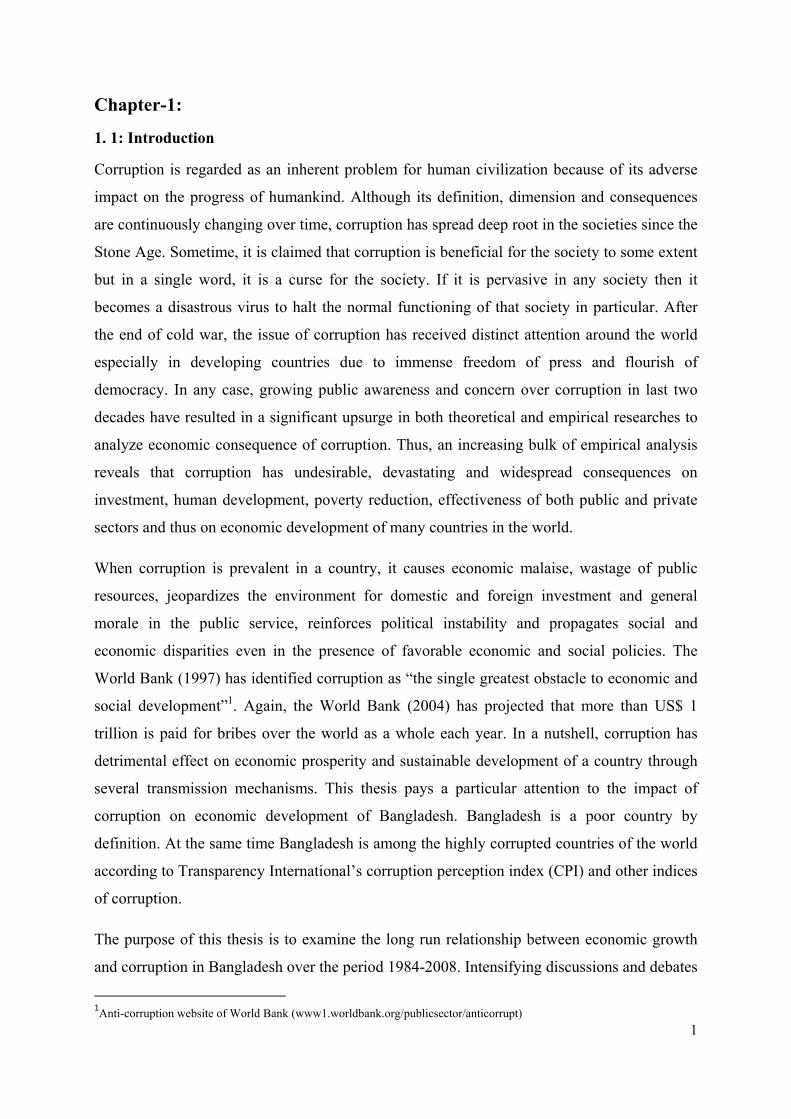
Howeve

classific

was US

populati

develop

that Ban

properly

               4Poverty

conomic De

desh is a ve

160 million

which resu

desh has do

e of major

nces. Figure

ntry during

ing its mac

empowerm

) despite of s

Figure-1

er, Banglad

cation of ec

S$462 in 20

ion in unde

pment comp

ngladesh wo

y utilize its

                      gap at $2 a da

evelopment

ery small a

n. About on

ulted into

one reasonab

expansion

e-1 illustrate

g 1993-2008

cro-econom

ment and lite

everal natura

: Growth

Sourc

desh falls int

conomic dev

008. Still t

er poverty li

pared to the

ould be able

economic c

                       ay (PPP) (%):

t and Corru

country in

ne fifth of e

slow econo

bly well in

in readym

es the trend

8. In recent

mic indicato

eracy rate a

al calamities

in real GD

ce: World B

to low-inco

velopment.

the standard

ine4. Moreo

countries w

e to improv

capabilities.

Source World

uption in B

South Asia

economy w

omic grow

accelerating

made garmen

d in real GD

t years, Ban

ors, reducin

nd in achiev

, political ins

P and GDP

Bank (WDI

ome categor

The countr

d of living

over, Bangla

with similar

ve its catego

d Bank -2005

Bangladesh

an region bu

was destroye

wth in the

g its GDP g

nts industry

DP growth a

ngladesh ha

ng the leve

ving other m

stability and

P per capita

Data Base-

ry country a

ry’s per cap

is very low

adesh is fal

characteris

ory into mid

: Some fact

ut having a

ed during th

following

growth durin

y and cont

and per cap

as performe

l of extrem

millennium

other draw b

a during 19

2010)

according to

pita GDP (c

w here and

ling behind

stics. But it

ddle income

ts

large popul

he liberation

years. Aft

ng last two

tribution of

ita GDP gro

ed relatively

me poverty,

m developme

backs.

993-2008.

o the World

constant 200

d about 34%

d in terms ec

is widely d

e by 2025 if

4 

lation of

n war in

fter that,

decades

f foreign

owth for

y well in

, raising

ent goals

d Bank’s

00 US$)

% of its

conomic

discussed

f it could

5  

In Bangladesh, corruption is considered as one of the major obstacles in the path economic

development. It has become rampant all over the society in this county since the independence

in 1971. In general, corruption is regarded somewhat obviously as 'a way of life' among the

mass people of Bangladesh. Re-establishment of parliamentary democracy from a dictatorial

military government in 1991 does not seem to have any influence on the nature and scope of

corruption. Corruption is a severe problem in the public sector of Bangladesh from an

international perspective also. Bangladesh had been ranked as the most corrupt country in

2001, 2002 and 2003 consecutively in Transparency International Corruption Perceptions

Index (CPI). According to the index of the International Country Risk Guide (ICRG),

Bangladesh was ranked as the sixth most corrupted nation out of the 123 nations of the world

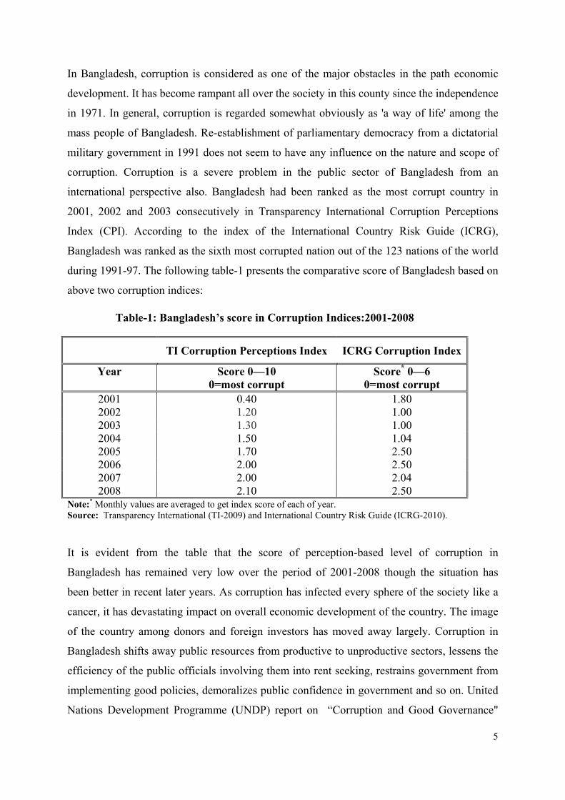
during 1991-97. The following table-1 presents the comparative score of Bangladesh based on

above two corruption indices:

It is evident from the table that the score of perception-based level of corruption in

Bangladesh has remained very low over the period of 2001-2008 though the situation has

been better in recent later years. As corruption has infected every sphere of the society like a

cancer, it has devastating impact on overall economic development of the country. The image

of the country among donors and foreign investors has moved away largely. Corruption in

Bangladesh shifts away public resources from productive to unproductive sectors, lessens the

efficiency of the public officials involving them into rent seeking, restrains government from

implementing good policies, demoralizes public confidence in government and so on. United

Nations Development Programme (UNDP) report on “Corruption and Good Governance"

Table-1: Bangladesh’s score in Corruption Indices:2001-2008

TI Corruption Perceptions Index ICRG Corruption Index

Year Score 0—10

0=most corrupt

Score* 0—6

0=most corrupt

2001 0.40 1.80 2002 1.20 1.00 2003 1.30 1.00 2004 1.50 1.04 2005 1.70 2.50 2006 2.00 2.50 2007 2.00 2.04 2008 2.10 2.50

Note:* Monthly values are averaged to get index score of each of year.

Source: Transparency International (TI-2009) and International Country Risk Guide (ICRG-2010).

 

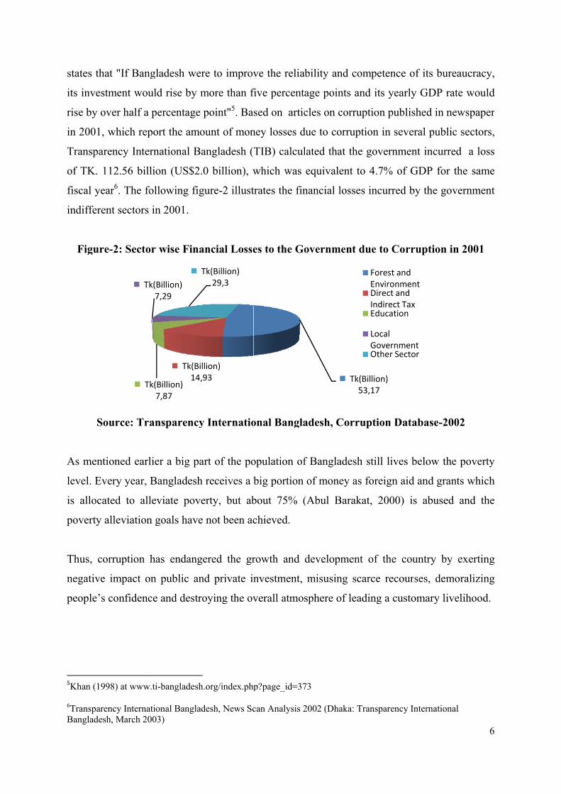
states th

its inves

rise by o

in 2001

Transpa

of TK.

fiscal ye

indiffere

Figur

S

As men

level. E

is alloc

poverty

Thus, c

negative

people’

               5Khan (19

6TransparBanglade

hat "If Bang

stment wou

over half a p

, which rep

arency Inter

112.56 bill

ear6. The fo

ent sectors i

re-2: Sector

Source: Tra

ntioned earli

very year, B

cated to alle

y alleviation

corruption h

e impact on

s confidenc

                      998) at www.

rency Internatesh, March 20

Tk

Tk

gladesh wer

uld rise by m

percentage

port the amo

rnational Ba

ion (US$2.

ollowing fig

in 2001.

r wise Fina

ansparency

ier a big pa

Bangladesh

eviate pove

goals have

has endang

n public an

ce and destro

                       ti-bangladesh

tional Banglad03)

Tk(Bil

14,k(Billion)

7,87

k(Billion)

7,29

T

re to improv

more than f

point"5. Ba

ount of mon

angladesh (

0 billion), w

gure-2 illust

ancial Losse

y Internatio

art of the po

receives a b

erty, but ab

not been ac

ered the gr

nd private in

oying the ov

h.org/index.php

desh, News Sc

lion)

93

Tk(Billion)

29,3

ve the relia

five percent

sed on artic

ney losses d

TIB) calcul

which was

trates the fin

es to the Go

onal Bangla

opulation of

big portion

bout 75% (

chieved.

rowth and

nvestment,

verall atmo

p?page_id=37

can Analysis 2

ability and c

age points a

cles on corr

due to corru

lated that th

equivalent

nancial loss

overnment

adesh, Cor

f Banglades

of money a

(Abul Bara

developmen

misusing s

sphere of le

73

2002 (Dhaka:

T

competence

and its year

ruption publ

uption in sev

he governm

to 4.7% of

ses incurred

t due to Cor

ruption Da

sh still lives

as foreign a

akat, 2000)

nt of the c

scarce recou

eading a cus

Transparency

k(Billion)

53,17

Forest anEnvironmDirect andIndirect TEducation

Local GovernmOther Sec

of its bure

rly GDP rat

lished in ne

veral public

ment incurred

f GDP for t

d by the gov

rruption in

atabase-200

s below the

id and gran

is abused

country by

urses, demo

stomary live

y International

d mentd Taxn

entctor

6 

eaucracy,

te would

ewspaper

c sectors,

d a loss

the same

vernment

n 2001

02

poverty

nts which

and the

exerting

oralizing

elihood.

l

7  

Chapter- 2: Review of previous literatures

This chapter is designed to give an overview of the earlier research works on corruption.

Although theoretical and empirical research on investigating the relation between corruption

and economic development is relatively a new arena in modern economics, there exists a vast

literature on this field7. Research on corruption has attracted immense importance since the

early 1990’s among the economists because it has widespread consequences on economic

development8. Most of the empirical works are either cross sectional or based on panel data

while there is probably no study yet using pure time series data for a single country.

Although there is a budding consensus that corruption is detrimental to the society, theories

concerning the influence of corruption have been conflicting to some extents. Some studies

have found that corruption works as lubricant to increase the speed of wheels of economic

activity and thus accelerates economic growth. Inspired by Leff (1964) and Huntington

(1968), this school of thought claims that corruption is beneficial in a sense that bribes act as

speed money for the entrepreneurs and businessmen to avoid bureaucratic delays and

cumbersome rules and regulations in investment mechanisms. For example, in an equilibrium

queuing model Lui(1985) suggest that efficiency of the public administration improves as

bribing tactics to reduce waiting costs form a non co-operative Nash equilibrium game

among businessmen. Again, competition among public officials can also reduce corruption

(Rose-Ackerman, 1978). On the other hand, many studies have claimed that corruption is a

hindrance to development as it slows down the pace economic activity by exerting negative

externalities through its long-lasting effect in the economic environment. This opposite strand

to the speed money proposition claims that corrupt practices between public administration

and investors are very detrimental to the overall economic prosperity as it undesirably affects

the quality and quantity of investment. Shleifer and Vishny (1993) point out that corruption is

more distortionary than taxation and is responsible for raising the cost of doing business,

which in turn impedes economic growth. Because it is illegal and it must be kept secret to

evade detection and penalty. Moreover, corrupt government officials in poor countries are

always interested to spend much resource on military and infrastructure where the scope on

                                                            7Bardhan.P( 1997), Lambsdorff, J. G.(1999), Jain (2001) and Adit (2003 )provide extensive review on empirical

literatures of corruption.

8 See Figure-A1 in the appendix-1which displays the studies on the consequences of corruption during1995-

2005.

8  

corruption is vast rather than spending on education and health. In a very famous paper

Murphy, Shleifer and Vishny (1993) give evidence that the pace of development of country is

usually halted when talented people are involved in rent seeking activities. In order to get a

clear overview of previous studies on the affect of corruption on economic development, I

have divided the discussion as underneath.

2. 1 Corruption and Economic Growth

Most of the empirical studies that investigate the direct relationship between corruption and

economic growth have found that pace of economic growth rate is slowed down due to

corruption9. The problem associated with this kind of research is the direction of causality

between corruption and economic growth. Lambsdorff (1999) in his review of literature

argues that low GDP per capita can cause corruption while opposite might be true. Mauro

initiated the systemic study on the corruption and growth using econometric tools in 1995.

Following Solow-Barro style cross-country growth regression framework, he studied the

relationship between corruption and economic growth using Business International (BI)

corruption index. He found substantial negative association between corruption and the

average annual economic growth rate over the period of 1960-85for 70 countries. With the

help of Lucas type model Brunetti (1997) gives evidence that corruption has negative

insignificant impact on growth .In an environment of less effective government and fragile

rule of law corruption is even more harmful for economic growth. Ehrlich and Lui (1999)

claimed that economic growth rate is lower due corruption (which is a result of higher level of

government intervention).Again, Mo (2001) has shown that corruption reduces economic

growth through human capital and political instability channels. His study reveals that 1% rise

in the corruption level decreases the growth rate by about 0.72%. Furthermore, in a similar

kind of study Pellegrini and Gerlagh (2005) catch that corruption substantially impacts

economic growth and income over time. Nevertheless, the negative effect is not always

evident in empirical studies. For example Barreto (2001), replicating Mauro (1995) has

proved that there exists a direct positive relation between growth and corruption. More

specifically, some East Asian countries have performed well to sustain a good GDP growth

rate in spite of high perceived level of corruption (Rock and Bonnett, 2004). Augmenting the

                                                            9Mauro (1995,1997), Brunetti, (1997), Poirson, (1998), Ehrlich and Lui, (1999),Li, Xu and Zou (2000), Mo (2001), Abed

and Davoodi (2002), Leite and Weidmann (2002) and Meon and Sekkat (2005) have found that corruption hurts economic

development.

 

9  

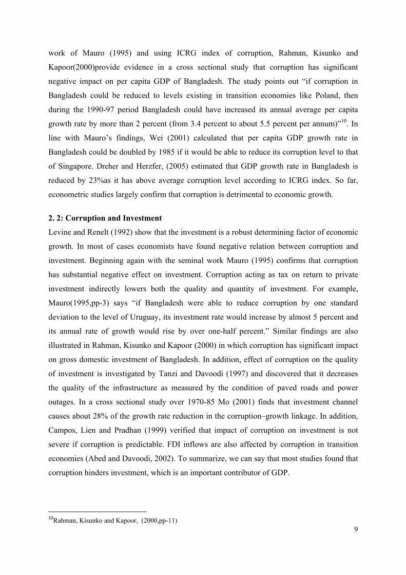
work of Mauro (1995) and using ICRG index of corruption, Rahman, Kisunko and

Kapoor(2000)provide evidence in a cross sectional study that corruption has significant

negative impact on per capita GDP of Bangladesh. The study points out “if corruption in

Bangladesh could be reduced to levels existing in transition economies like Poland, then

during the 1990-97 period Bangladesh could have increased its annual average per capita

growth rate by more than 2 percent (from 3.4 percent to about 5.5 percent per annum)”10. In

line with Mauro’s findings, Wei (2001) calculated that per capita GDP growth rate in

Bangladesh could be doubled by 1985 if it would be able to reduce its corruption level to that

of Singapore. Dreher and Herzfer, (2005) estimated that GDP growth rate in Bangladesh is

reduced by 23%as it has above average corruption level according to ICRG index. So far,

econometric studies largely confirm that corruption is detrimental to economic growth.

2. 2: Corruption and Investment

Levine and Renelt (1992) show that the investment is a robust determining factor of economic

growth. In most of cases economists have found negative relation between corruption and

investment. Beginning again with the seminal work Mauro (1995) confirms that corruption

has substantial negative effect on investment. Corruption acting as tax on return to private

investment indirectly lowers both the quality and quantity of investment. For example,

Mauro(1995,pp-3) says “if Bangladesh were able to reduce corruption by one standard

deviation to the level of Uruguay, its investment rate would increase by almost 5 percent and

its annual rate of growth would rise by over one-half percent.” Similar findings are also

illustrated in Rahman, Kisunko and Kapoor (2000) in which corruption has significant impact

on gross domestic investment of Bangladesh. In addition, effect of corruption on the quality

of investment is investigated by Tanzi and Davoodi (1997) and discovered that it decreases

the quality of the infrastructure as measured by the condition of paved roads and power

outages. In a cross sectional study over 1970-85 Mo (2001) finds that investment channel

causes about 28% of the growth rate reduction in the corruption–growth linkage. In addition,

Campos, Lien and Pradhan (1999) verified that impact of corruption on investment is not

severe if corruption is predictable. FDI inflows are also affected by corruption in transition

economies (Abed and Davoodi, 2002). To summarize, we can say that most studies found that

corruption hinders investment, which is an important contributor of GDP.

                                                            10

Rahman, Kisunko and Kapoor, (2000,pp-11) 

10  

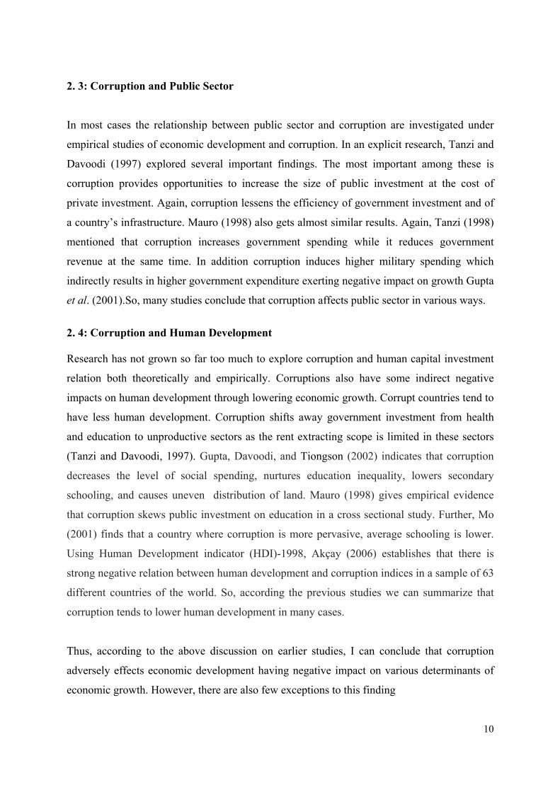
2. 3: Corruption and Public Sector

In most cases the relationship between public sector and corruption are investigated under

empirical studies of economic development and corruption. In an explicit research, Tanzi and

Davoodi (1997) explored several important findings. The most important among these is

corruption provides opportunities to increase the size of public investment at the cost of

private investment. Again, corruption lessens the efficiency of government investment and of

a country’s infrastructure. Mauro (1998) also gets almost similar results. Again, Tanzi (1998)

mentioned that corruption increases government spending while it reduces government

revenue at the same time. In addition corruption induces higher military spending which

indirectly results in higher government expenditure exerting negative impact on growth Gupta

et al. (2001).So, many studies conclude that corruption affects public sector in various ways.

2. 4: Corruption and Human Development

Research has not grown so far too much to explore corruption and human capital investment

relation both theoretically and empirically. Corruptions also have some indirect negative

impacts on human development through lowering economic growth. Corrupt countries tend to

have less human development. Corruption shifts away government investment from health

and education to unproductive sectors as the rent extracting scope is limited in these sectors

(Tanzi and Davoodi, 1997). Gupta, Davoodi, and Tiongson (2002) indicates that corruption

decreases the level of social spending, nurtures education inequality, lowers secondary

schooling, and causes uneven distribution of land. Mauro (1998) gives empirical evidence

that corruption skews public investment on education in a cross sectional study. Further, Mo

(2001) finds that a country where corruption is more pervasive, average schooling is lower.

Using Human Development indicator (HDI)-1998, Akçay (2006) establishes that there is

strong negative relation between human development and corruption indices in a sample of 63

different countries of the world. So, according the previous studies we can summarize that

corruption tends to lower human development in many cases.

Thus, according to the above discussion on earlier studies, I can conclude that corruption

adversely effects economic development having negative impact on various determinants of

economic growth. However, there are also few exceptions to this finding

11  

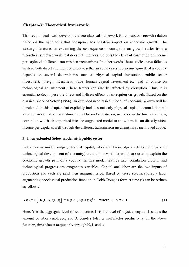
Chapter-3: Theoretical framework

This section deals with developing a neo-classical framework for corruption- growth relation

based on the hypothesis that corruption has negative impact on economic growth. The

existing literatures on examining the consequence of corruption on growth suffer from a

theoretical structure work that does not includes the possible effect of corruption on income

per capita via different transmission mechanisms. In other words, these studies have failed to

analyze both direct and indirect effect together in some cases. Economic growth of a country

depends on several determinants such as physical capital investment, public sector

investment, foreign investment, trade ,human capital investment etc. and of course on

technological advancement. These factors can also be affected by corruption. Thus, it is

essential to decompose the direct and indirect effects of corruption on growth. Based on the

classical work of Solow (1956), an extended neoclassical model of economic growth will be

developed in this chapter that explicitly includes not only physical capital accumulation but

also human capital accumulation and public sector. Later on, using a specific functional form,

corruption will be incorporated into the augmented model to show how it can directly affect

income per capita as well through the different transmission mechanisms as mentioned above.

3. 1: An extended Solow model with public sector

In the Solow model, output, physical capital, labor and knowledge (reflects the degree of

technological development of a country) are the four variables which are used to explain the

economic growth path of a country. In this model savings rate, population growth, and

technological progress are exogenous variables. Capital and labor are the two inputs of

production and each are paid their marginal price. Based on these specifications, a labor

augmenting neoclassical production function in Cobb-Douglas form at time (t) can be written

as follows:

α 1-α(t) (t) (t) (t) (t) (t) (t)Y = F (K ,A L = K (A L ) where, 0 < α< 1 (1)

Here, Y is the aggregate level of real income, K is the level of physical capital, L stands the

amount of labor employed, and A denotes total or multifactor productivity. In the above

function, time affects output only through K, L and A.

12  

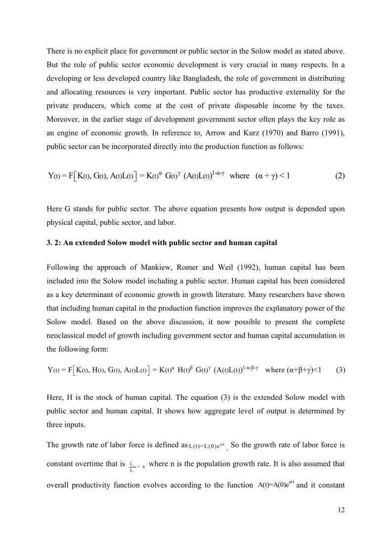
There is no explicit place for government or public sector in the Solow model as stated above.

But the role of public sector economic development is very crucial in many respects. In a

developing or less developed country like Bangladesh, the role of government in distributing

and allocating resources is very important. Public sector has productive externality for the

private producers, which come at the cost of private disposable income by the taxes.

Moreover, in the earlier stage of development government sector often plays the key role as

an engine of economic growth. In reference to, Arrow and Kurz (1970) and Barro (1991),

public sector can be incorporated directly into the production function as follows:

α γ 1-α-γ(t) (t) (t (t) (t) (t) (t) (t) (t) )Y = F K , G , A L = K G (A L ) where (α + γ) < 1 (2)

Here G stands for public sector. The above equation presents how output is depended upon

physical capital, public sector, and labor.

3. 2: An extended Solow model with public sector and human capital

Following the approach of Mankiew, Romer and Weil (1992), human capital has been

included into the Solow model including a public sector. Human capital has been considered

as a key determinant of economic growth in growth literature. Many researchers have shown

that including human capital in the production function improves the explanatory power of the

Solow model. Based on the above discussion, it now possible to present the complete

neoclassical model of growth including government sector and human capital accumulation in

the following form:

β γ 1-α-β-γα(t) (t) (t) (t) (t) (t) (t) (t) (t) (t) (t)Y = F K , H , G , A L = K H G (A L ) where (α+β+γ)<1 (3)

Here, H is the stock of human capital. The equation (3) is the extended Solow model with

public sector and human capital. It shows how aggregate level of output is determined by

three inputs.

The growth rate of labor force is defined as n tL (t)= L (0 )e . So the growth rate of labor force is

constant overtime that is .

L= n

L

where n is the population growth rate. It is also assumed that

overall productivity function evolves according to the function t

A(t)=A(0)e

and it constant

13  

over time that is

.

A=

A where ϖ is the growth rate of technological progress. Here,

(α+β+γ)<1 implies that production function exhibits decreasing returns to each input. Now the

intensive form of production function can be written as below:

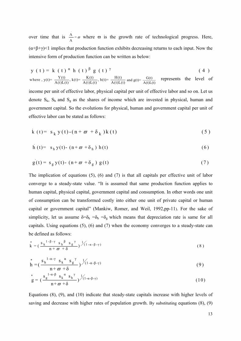
β γαy ( t ) = k ( t ) h ( t ) g ( t ) ( 4 )

Y(t) K(t) H(t)where , y(t)= , k(t)= , h(t)=

A(t)L(t) A(t)L(t) A(t)L(t)

G(t)and g(t)=

A(t)L(t) represents the level of

income per unit of effective labor, physical capital per unit of effective labor and so on. Let us

denote Sk, Sh and Sg as the shares of income which are invested in physical, human and

government capital. So the evolutions for physical, human and government capital per unit of

effective labor can be stated as follows:

.

k k k ( t ) = s y ( t ) - ( n + + δ ) k ( t ) ( 5 )

.

h h h ( t )= s y ( t )- (n + + δ ) h ( t) (6 )

.

g g g ( t ) = s y ( t ) - (n + + δ ) g ( t ) (7 )

The implication of equations (5), (6) and (7) is that all capitals per effective unit of labor

converge to a steady-state value. “It is assumed that same production function applies to

human capital, physical capital, government capital and consumption. In other words one unit

of consumption can be transformed costly into either one unit of private capital or human

capital or government capital” (Mankiw, Romer, and Weil, 1992,pp-11). For the sake of

simplicity, let us assume δ=δk =δh =δg which means that depreciation rate is same for all

capitals. Using equations (5), (6) and (7) when the economy converges to a steady-state can

be defined as follows:

1 -β - γ β γ 1* gk h ( 1 -α -β - γ )s s sk = ( ) ( 8 )

n + + δ

1 -α -γ α γ 1*h k g (1 -α -β -γ )

s s sh = ( ) (9 )

n + + δ1-α -β α γ 1*

g k h (1-α -β -γ)s s s

g = ( ) (10)n+ +δ

Equations (8), (9), and (10) indicate that steady-state capitals increase with higher levels of

saving and decrease with higher rates of population growth. By substituting equations (8), (9)

14  

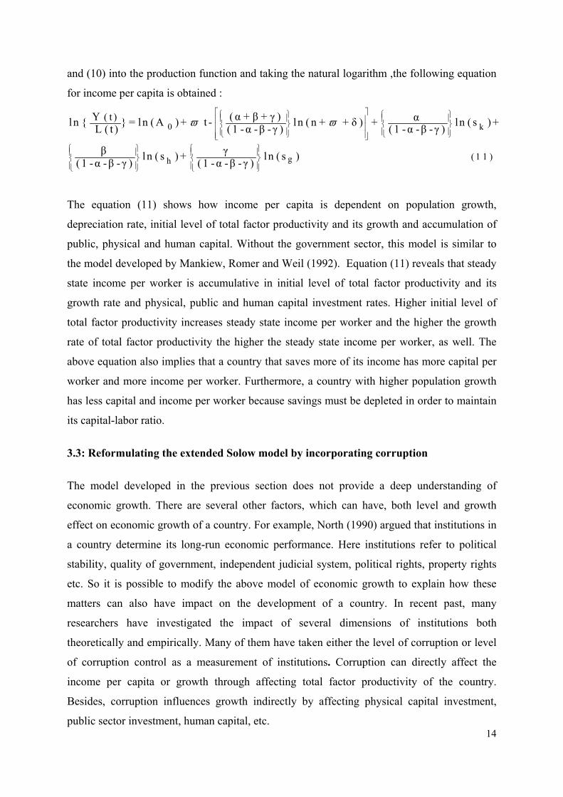
and (10) into the production function and taking the natural logarithm ,the following equation

for income per capita is obtained :

0 k

gh ( 1 1

( t ) (α + β + γ )Y αln { } = ln ( A ) + t - ln ( n + + δ ) + ln ( s ) + L ( t ) ( 1 -α -β -γ ) ( 1 -α -β -γ )

β γln ( s ) + ln ( s )

( 1 -α -β -γ ) ( 1 -α -β -γ )

)

The equation (11) shows how income per capita is dependent on population growth,

depreciation rate, initial level of total factor productivity and its growth and accumulation of

public, physical and human capital. Without the government sector, this model is similar to

the model developed by Mankiew, Romer and Weil (1992). Equation (11) reveals that steady

state income per worker is accumulative in initial level of total factor productivity and its

growth rate and physical, public and human capital investment rates. Higher initial level of

total factor productivity increases steady state income per worker and the higher the growth

rate of total factor productivity the higher the steady state income per worker, as well. The

above equation also implies that a country that saves more of its income has more capital per

worker and more income per worker. Furthermore, a country with higher population growth

has less capital and income per worker because savings must be depleted in order to maintain

its capital-labor ratio.

3.3: Reformulating the extended Solow model by incorporating corruption

The model developed in the previous section does not provide a deep understanding of

economic growth. There are several other factors, which can have, both level and growth

effect on economic growth of a country. For example, North (1990) argued that institutions in

a country determine its long-run economic performance. Here institutions refer to political

stability, quality of government, independent judicial system, political rights, property rights

etc. So it is possible to modify the above model of economic growth to explain how these

matters can also have impact on the development of a country. In recent past, many

researchers have investigated the impact of several dimensions of institutions both

theoretically and empirically. Many of them have taken either the level of corruption or level

of corruption control as a measurement of institutions. Corruption can directly affect the

income per capita or growth through affecting total factor productivity of the country.

Besides, corruption influences growth indirectly by affecting physical capital investment,

public sector investment, human capital, etc.

15  

Let us first concentrate on the discussion of the direct impact of corruption on growth in the

light of the augmented Solow model derived above. Total factor productivity (TFP) growth

measures the changes in output not caused by changes in inputs. TFP growth explains the

effect of technological change, efficiency improvements, and our inability to measure directly

the contribution of all other inputs. Therefore, it is reasonable to assume that corruption

reduces the efficiency gain from technological advancement by imposing negative externality

on it. Countries with high level of corruption gain less benefit from technological

advancement. In order to show the direct of corruption via total factor productivity a structural

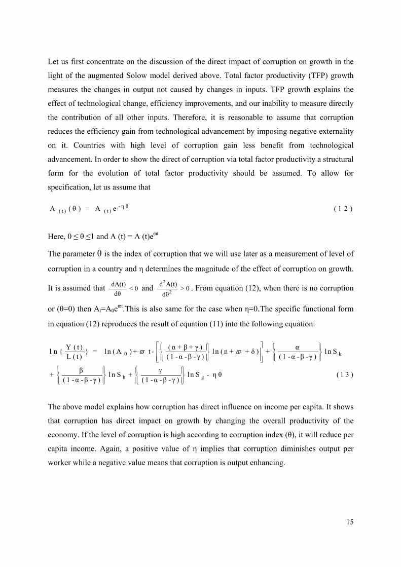
form for the evolution of total factor productivity should be assumed. To allow for

specification, let us assume that

- η θ( t ) ( t )A ( θ ) = A e ( 1 2 )

Here, 0 ≤ θ ≤1 and A (t) = A (t)eϖt

The parameter θ is the index of corruption that we will use later as a measurement of level of

corruption in a country and η determines the magnitude of the effect of corruption on growth.

It is assumed that dA(t)

< 0dθ

and 2

2

d A(t)> 0

dθ. From equation (12), when there is no corruption

or (θ=0) then At=A0eϖt.This is also same for the case when η=0.The specific functional form

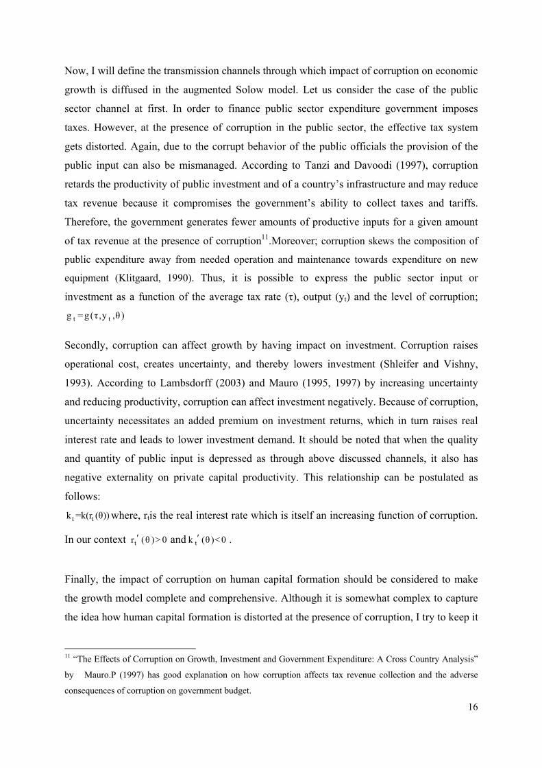
in equation (12) reproduces the result of equation (11) into the following equation:

0 k

gh

Y ( t ) (α + β + γ ) αl n { } = ln ( A ) + t - ln ( n + + δ ) + ln S

L ( t ) ( 1 -α -β -γ ) ( 1 -α -β -γ )

β γ+ ln S + ln S - η θ ( 1 3 )

( 1 -α -β - γ ) ( 1 -α -β -γ )

The above model explains how corruption has direct influence on income per capita. It shows

that corruption has direct impact on growth by changing the overall productivity of the

economy. If the level of corruption is high according to corruption index (θ), it will reduce per

capita income. Again, a positive value of η implies that corruption diminishes output per

worker while a negative value means that corruption is output enhancing.

16  

Now, I will define the transmission channels through which impact of corruption on economic

growth is diffused in the augmented Solow model. Let us consider the case of the public

sector channel at first. In order to finance public sector expenditure government imposes

taxes. However, at the presence of corruption in the public sector, the effective tax system

gets distorted. Again, due to the corrupt behavior of the public officials the provision of the

public input can also be mismanaged. According to Tanzi and Davoodi (1997), corruption

retards the productivity of public investment and of a country’s infrastructure and may reduce

tax revenue because it compromises the government’s ability to collect taxes and tariffs.

Therefore, the government generates fewer amounts of productive inputs for a given amount

of tax revenue at the presence of corruption11.Moreover; corruption skews the composition of

public expenditure away from needed operation and maintenance towards expenditure on new

equipment (Klitgaard, 1990). Thus, it is possible to express the public sector input or

investment as a function of the average tax rate (τ), output (yt) and the level of corruption;

t tg = g(τ ,y ,θ )

Secondly, corruption can affect growth by having impact on investment. Corruption raises

operational cost, creates uncertainty, and thereby lowers investment (Shleifer and Vishny,

1993). According to Lambsdorff (2003) and Mauro (1995, 1997) by increasing uncertainty

and reducing productivity, corruption can affect investment negatively. Because of corruption,

uncertainty necessitates an added premium on investment returns, which in turn raises real

interest rate and leads to lower investment demand. It should be noted that when the quality

and quantity of public input is depressed as through above discussed channels, it also has

negative externality on private capital productivity. This relationship can be postulated as

follows:

t tk =k(r (θ)) where, rtis the real interest rate which is itself an increasing function of corruption.

In our context tr (θ )> 0 and tk (θ )< 0 .

Finally, the impact of corruption on human capital formation should be considered to make

the growth model complete and comprehensive. Although it is somewhat complex to capture

the idea how human capital formation is distorted at the presence of corruption, I try to keep it

                                                            11 “The Effects of Corruption on Growth, Investment and Government Expenditure: A Cross Country Analysis”

by Mauro.P (1997) has good explanation on how corruption affects tax revenue collection and the adverse

consequences of corruption on government budget.

17  

as simple as possible. Corruption distorts the allocation of resources in human capital

formation and quality of human capital investment also. According to Mauro (1998), public

officials do not want to spend more on education and health because this spending programme

offers less opportunity for rent seeking. Gupta, Davoodi, and Tiongson (2000) conclude that

corruption has negative impact on health care and education services in two ways: (1)

corruption may raise the cost of these services, and (2) corruption may reduce the quality of

these services. Moreover, skilled and talented workforce engaged in rent seeking activities

which lowers the pace of human development. In this paper, I will only consider the case

where corruption affects human capital accumulation through its negative effect on

educational expenditure. The mechanism can be presented by assuming the following

functional form:

t th =h(EX (θ)) where EX (θ) shows that expenditure on education is a function of corruption and

EX (θ)<0

Based on the above arguments, the steady state equation for income per worker from equation

(13) including corruption for revealing both direct and indirect effect can be reproduced as

follows:

t

t

0 k ( r (θ ) )

g th ( E X (θ ) )

Y ( t ) (α + β + γ ) αl n { } = ln ( A ) + t - ln ( n + + δ ) + ln s

L ( t ) ( 1 -α -β -γ ) ( 1 -α -β -γ )

β γ+ ln s + ln s ( τ ,y ,θ ) -η θ ( 1 4 )

( 1 -α -β -γ ) ( 1 -α -β -γ )

Equation (14) illuminates both the direct and indirect impacts of corruption on the per capita

output over time. As an increase in corruption reduces total factor productivity, an increase in

the level corruption has an inverse relationship with growth of income per worker Corruption

also indirectly impacts per capita output growth by reducing the growth of physical capital,

human capital and diminishing the productive externality provided by the public sector. This

modeling approach has several advantages over the models used in the literature: i)

importantly, it builds on the well-known neoclassical growth model ii) the model allows the

use of the modern time series data methods in estimations iii) in addition the incorporation of

the growth effects of corruption into the model is done in a general way that captures both

direct and indirect effect of corruption.

18  

Chapter-4: Empirical framework, Data and Methodology

4. 1: Econometric Models

To achieve the main purpose of this research i.e. testing the existence of long run relationship

between economic growth and corruption and examining the direct and indirect consequences

of corruption on economic development in Bangladesh, I have used modern time series

econometric techniques for the period of 1984-2008. If there is a long run relationship(co-

integration), then I would estimate impact of corruption on economic growth. Therefore, this

chapter outlines the structure of econometric models designed and their relevance in the light

of the theoretical framework developed in the previous chapter. It is apparent from our

extended Solow model that income per capita depends on physical, public and human capital

accumulation. Thus, the following base model without corruption will be estimated at first:

t 0 1 t 2 t 3 t 4 t tl n Y = β + β l n I N V + β l n G V X + β l n E D X + β l n Z + u ( I )

t t tH e re , Z ln ( + δ+ n )

In the above specification, Y denotes Real GDP per capita, which is used as an alternative for

income per worker. In most of the empirical growth literatures, researchers use this as an

indicator of economic growth of a country. Gross fixed capital formation is used for

measuring physical capital formation, which is denoted by INV. Further, GVX stands

government final consumption expenditure, which is taken as proxy for public sector input,

and EDX indicates public expenditure on education, which is proxy for human capital

formation. Here, Z is used to denote the accumulation of total factor productivity growth rate

(ϖ), depreciation rate (δ) and population growth rate (n) as explained in theoretical frame

work. Lastly, u is the usual error term with classical properties and t stands for the time index.

Hence, the estimation of the above equation would be used to explain the long run

determinants of economic growth of Bangladesh. Based on the theoretical framework, it is

expected that the signs of coefficients of INV, GVX and EDX would be positive. The value of

each parameter associated with each variable will reflect the long run contribution of various

determinants of economic development.

19  

Adding corruption as an explanatory variable in the base model, it is possible to estimate the

effect of corruption on economic growth. Therefore, motivated by the theoretical model stated

in equation (14), the following empirical model will be estimated:

t 0 1 t 2 t 3 t 4 t 5 t t1lnY = β +β lnIN V +β lnG V X +β lnED X +β ln Z +β lnC O R +u (II)

Here, COR represents the index of corruption, which will be discussed in details in the next

section of this chapter. In order to avoid the problem of non-normality and interpretation, I

have multiplied the index corruption by hundred (100) and taken natural log of it. The

expected sign of corruption parameter is negative which would reflect the negative impact on

real GDP per capita or economic growth as derived in the theoretical model. It shows the

direct effect of corruption on per capita real GDP. By analyzing the signs and change in the

parameter value associated with the determinants of GDP, we would be able to understand

how corruption influences it through various channels. As priori, we can say that it will

decrease the parameter values as in equation (I).

4.2: The choice of indicators and their sources

This section provides a discussion of the choice of indicators used in this research paper and

their sources. Annual aggregate time series data for Bangladesh is used in this study which

consists of 25 observations for the period of 1984-2008. The sample size is relatively small

due to the unavailability of the data on the measurement of corruption for Bangladesh. But the

most important matter is that the most recent data has been used for this study. Real GDP per

capita (constant 2000 US$) is used as proxy for income per capita which is the dependent

variable in our empirical models. It is the value of all final goods and services produced

within the geographical area of a country during one-year period divided by consumer price

index. Gross fixed capital formation or investment comprises land improvements, plant,

machinery, and equipment purchases; and the construction of roads, railways, and the like,

including schools, offices, hospitals, private residential dwellings, and commercial and

industrial buildings12.Government final consumption expenditure consists all contemporary

government expense to buy goods and services including salaries of employees. Note that

military investment is not included in government final consumption expenditure. Public

expenditure on education is the government current expense on education sector. These three                                                             12

Definition of World Bank’s world development indicator (WDI-2008) database.

20  

variables are taken as a percentage share of GDP. Population growth rate is annual growth of

population in percentage term. I have assumed 3% (percentage) depreciation rate for all

capitals. The primary sources of these statistics are World Bank Development Indicators

(WDI) data base, Ministry of Education and Ministry of Finance Bangladesh, Bangladesh

Bank (Central Bank of Bangladesh) etc.

I have extracted data for total factor productivity (TFP) growth rate from the total economy

data base of the Conference Board13. According to their definition, TFP growth measures the

changes in output not produced by the changes in inputs. It can be technological

advancement, improvement in efficiency and many other factors which are not measurable. A

complete list of variables used in this paper including their sources and description is

provided in table-A1 in appendix-2.

I have chosen the corruption index of the International Country Risk Guide (ICRG) ratings

complied by the Political Risk Services (PRS) Group Inc. The prime reason for using this

index is that it has data on corruption date back to 1984 for Bangladesh. Again, this data base

is used extensively for researches in corruption, appearing recently in the empirical studies of

Knack and Keefer (1995), Tanzi and Davoodi (1997), Rahman, Kisunko and Kapoor (2000),

Dreherand Herzfel (2005)Seldadyo and Haan (2006) ,Wei (2000)and so on. According to

ICRG,this corruption index is an estimator of the degree of political corruption in a political

system. It is a subjective measure of corruption that ranges from “0” to “6”, with “0” being

the highest corrupt. This index is prepared on monthly basis. As all other variables used in

this study are yearly, I have transformed the monthly data in to yearly data by taking the

average at first. Secondly, for tranquil and simple interpretation of the empirical results and to

make it more intuitive, I have reversed the raw corruption data into an index ranging from “0”

to “1” where the higher the index the higher the level of average corruption. In a nutshell, the

proxy variable for corruption index is constructed in this way: tθ

C O R = ( 1 - )6

, Where CORt

stands for the measurement of corruption in the empirical analysis. Now-a-days, there are

several organizations which have constructed indices for measuring the level of corruption.

Except ICRG, these are Corruption Perception Index (CPI) by Transparency International,

Kaufman and Kraay’ index (KK), the Business International Index (BI) and the World

Economic Forum index (GCR). It should be noted that correlation among different corruption

                                                            13

The Conference Board Total Economy Database, January 2010, http://www.conference-

board.org/data/economydatabase/

21  

indices are high (see table-A2 in appendix-2). Although these quantifiable measures that are

widely used by researchers to link economic performance with corruption, the main

limitations of the majority of these measures are their heavy bias towards the perception of

foreign investors and experts, their poll-based nature and restricted coverage.

4. 3: Regression Techniques

There are a number of methods available to examine the existence of long run equilibrium

relationship or the co-integration among the time series variables. The most common

techniques are residual based Engle-Granger (1987) two-step and one step procedures and

Johansen (1988), Johansen and Juselius (1990) test for co-integration based on maximum

likelihood method. However, there are several major disadvantages associated with these

methods. For instance, Enders (2004) proved that variables must be integrated in the same

order by definition for co-integration in Engle-Granger procedure. These two methods for

finding the co-integration are not that much reliable for studies with small sample size. This

research work adopts relatively a new technique for testing the existence of a co-integration

which developed in a series of studies by Pesaran and Shin (1995a,1995b) and Pesaran, Shin

and Smith (1996,2001)known as Auto-Regressive Distributed Lag (ARDL) Bounds Test

methodology.

The bounds testing approach has certain econometric advantages in comparison to other co-

integration procedures, According Pesaran(1997), the ARDL procedure yields precise

estimates of long run parameters and valid t-statistics even in the presence of endogenous

variables. In line with Banerjee et al. (1993), the error correction model (ECM) can be

derived from the ARDL through a simple liner transformation. In addition, the ARDL

approach to test for the existence of a long-run relationship among the variables is applicable

regardless of whether the underlying regressors are purely I(0), purely I(1), or mutually

integrated. Finally, according to Narayan (2005), the small sample properties of the bounds

testing approach are far superior to that of multivariate co-integration14. So considering all the

above mentioned points and based on the theory that per capita GDP in dependent on

                                                            14In particular, Pesaran and Shin (1999) show that the ARDL approach has better properties in sample sizes up to

150 observations

22  

investment, government expenditure and educational expenditure the unconditional ARDL–

ECM representation of the empirical equation (I) can be designed as follows:

1 2 2 2

p

t 50 1 t-1 2 t-1 3 t-1 4 t-1 t-1 i t-ii= 1

q q q q

ti t-i t-i t-i i t-ii= 0 i 0 i 0 i= 0

ln Y =β +λ lnY +λ ln IN V λ lnG V X λ lnE D X λ lnZ η lnΔY

+ θ Δ ln IN V lnG V X lnE D X γ Δ lnZ + u (I.a)i i

Where β0 is the constant and tu is the white noise error term. The terms associated with

summation signs denote the short run dynamics, whereas λis are the long run multipliers. In

order to maintain consistency, the bounds test must be executed on the second model (II) also.

Because of adding corruption as an independent variable in the model, co-integration may not

be found or vice-verse. The equations for the model with corruption are given in Appendix-3.

The first step in the ARDL bounds test approach is to estimate equation (I.a) by ordinary least

square (OLS) method. The regression results of the full model are of no interest. An F-test is

performed to test the presence of long run relationship among the variables. The null

hypothesis of non-existence of long run relationship in equation (I.a) o 1 2 3 4 5H :λ =λ =λ =λ =λ =0 is

tested against the alternative hypothesis of co-integration o 1 2 3 4 5H : λ 0,λ 0,λ 0,λ 0,λ 0, 0 .

However, the asymptotic distribution of this F-statistic is nonstandard, depending on the

regressors whether they are I (0) or I (1). It rests on the number of regressors and whether the

ARDL model comprises an intercept and/or trend. If the computed F-statistic is greater than

the upper critical value, the null hypothesis of no long-run relationship (No Co-integration)

can be rejected irrespective of the orders of integration for the time series. On the contrary, if

the test statistic is less than the lower critical value the null hypothesis cannot be rejected.

However, if the test statistics lies between the lower and upper critical values, no conclusion

regarding co-integration can be made. Two sets of critical values are provided in Pesaran and

Pesaran (1997) and in Pesaran et al. (2001).These critical values are generated on sample

sizes of 500 and 1000 observations and 20,000 and 40,000 replications, respectively.

However, Narayan (2005) argue that such critical values cannot be used for small sample

sizes like the one in this study.15 Given the relatively small sample size in the present study

                                                            15

For instance, he makes a comparison of the critical values generated with 31 observations and the critical

values in Pesaran et al. (2001) and finds that the upper bound CV at the 5% significance level for 31

observations with 4 regressors is 18.3% lower than the CV for 31 observations

 

23  

(25 observations); I extract the appropriate critical values from Narayan (2005) which were

generated for small sample sizes of between 30 and 80 observations. The appropriate lag

length for the model can be selected on the basis Schawrtz-Bayesian Criteria (SBC) and

Akaike Information Criteria (AIC) or any other information criterion. After finding a long run

relationship (co-integration) among the variables, the following the conditional ARDL (p, q1,

q2, q3, q4) long run model for Yt is estimated in the second step:

31 2 4qq q qp

t t0 21i t-i i t-i 3i t-i 4i t-i 5i t-ii=1 i=0 i=0 i 0 i=0

lnY =β λ lnY + λ lnINV λ lnGVX λ lnEDX λ lnZ +u (I.b)

Following the same procedure, the long run model adding corruption as an independent

variable can be estimated. In the third and final step, we obtain the short-run dynamic

parameters by estimating an error correction model (ECM) associated with the long-run

estimates. This is specified as below:

31 2 4qq q qp

t 0 i t-i i t-i t-i t-i i t-i t-1 ti=1 i=0 i 0 i 0 i=0

lnY =β + η lnY + θ ΔlnINV lnGVX lnEDX γ ΔlnZ υECM +u (I.c)i i

Here, the most important point should be kept in mind that the sign of the error correction

term must be negative. All coefficients of the short run equation (I.c) are coefficients relating

to the short run dynamics of the models convergence to equilibrium and υ represents the

speed of adjustment for short run divergence to the long run equilibrium. It shows how

disequilibrium of the previous year’s shock adjusts back to the long run equilibrium in the

current year.

Last of all, in order to ascertain that the estimated models do not suffer from serial correlation,

non-normality and heteroscidasticity, I have performed Ljung-Box test, Jarque–Bera test and

Shapiro–Wilk test and ARCH test respectively in each model. Moreover, even in the presence

of co-integration, the results will be erratic, if the parameters are not constant. In order to test

for long-run parameter stability, Pesaran and Pesaran (1997) suggest applying the cumulative

sum of recursive residuals (CUSUM) test proposed by Brown et al (1975) to the residuals of

the estimated ARDL-ECMs to test for parameter constancy.

24  

Chapter-5: Contemporaneous correlation and graphical analyses

Before moving to formal empirical analysis, it is a good idea to show the relationship among

the variables using contemporaneous correlation and graphical analysis. Although correlation

matrix cannot give us the exact relationship among the variables of this study,

contemporaneous correlation among all the variables has been calculated in the following

table-2 in order to understand how the variables are moving and how these are correlated.

It is evident that the contemporaneous correlation between Y and the level of INV, GVX and

EDX is positive and very high. It is also noticeable total factor productivity growth rate and

real per capita GDP is positively correlated though the magnitude is low. We can see that

correlation between GDP per capita and corruption is negative which is -0.58.There also exist

negative correlation between the level of corruption and the determinants of economic

growth. For example, investment and corruption has a negative correlation by the magnitude

of 0.63. The relationship among other variables is not that much important here. Graphical

presentation is another to describe data systematically. The plot of underlying variables in

natural logarithmic form is depicted in figure-1 on the next page. Guided by the theoretical

explanation I have constructed a new variable denoted by Z by adding up total factor

productivity, population growth and depreciation rates. There is clearly an increasing trend in

real GDP per capita which indicates Bangladesh has maintained a good growth rate during the

last two decades. Investment and public education expenditure is also increasing with very

little fluctuations. As illustrated in the figure-3, government final consumption series has also

Table-2: Correlation Matrix among the variables in levels

Variables Y N TFP INV GVX EDX COR

Y 1.00

N -0.95 1.00

TFP 0.45 -0.49 1.00

INV 0.94 -0.95 0.45 1.00

GVX 0.87 -0.85 0.43 0.82 1.00

EDX 0.85 -0.94 0.49 0.95 0.71 1.00

COR -0.58 0.73 -0.71 -0.63 -0.46 -0.77 1.00

 

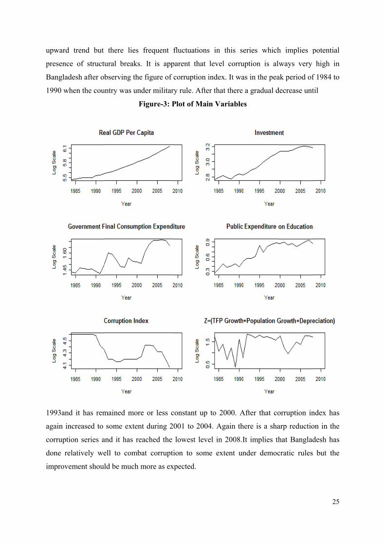
upward

presenc

Banglad

1990 wh

1993and

again in

corrupti

done re

improve

trend but

e of structu

desh after ob

hen the cou

d it has rem

ncreased to

ion series a

elatively we

ement shoul

there lies

ural breaks

bserving th

untry was un

F

mained mor

some exten

and it has re

ell to comb

ld be much

frequent f

s. It is app

e figure of c

nder military

Figure-3: P

re or less c

nt during 20

eached the

bat corrupti

more as ex

fluctuations

parent that

corruption i

y rule. Afte

Plot of Mai

constant up

001 to 2004

lowest leve

ion to som

pected.

s in this se

level corru

index. It wa

er that there

n Variable

to 2000. A

4. Again th

el in 2008.I

me extent un

eries which

uption is al

as in the pea

a gradual d

es

After that co

here is a sha

It implies th

nder democ

h implies p

lways very

ak period of

decrease unt

orruption in

arp reductio

hat Banglad

cratic rules

25 

potential

high in

f 1984 to

til

ndex has

on in the

desh has

but the

26  

Chapter-6: Presentation of the empirical results

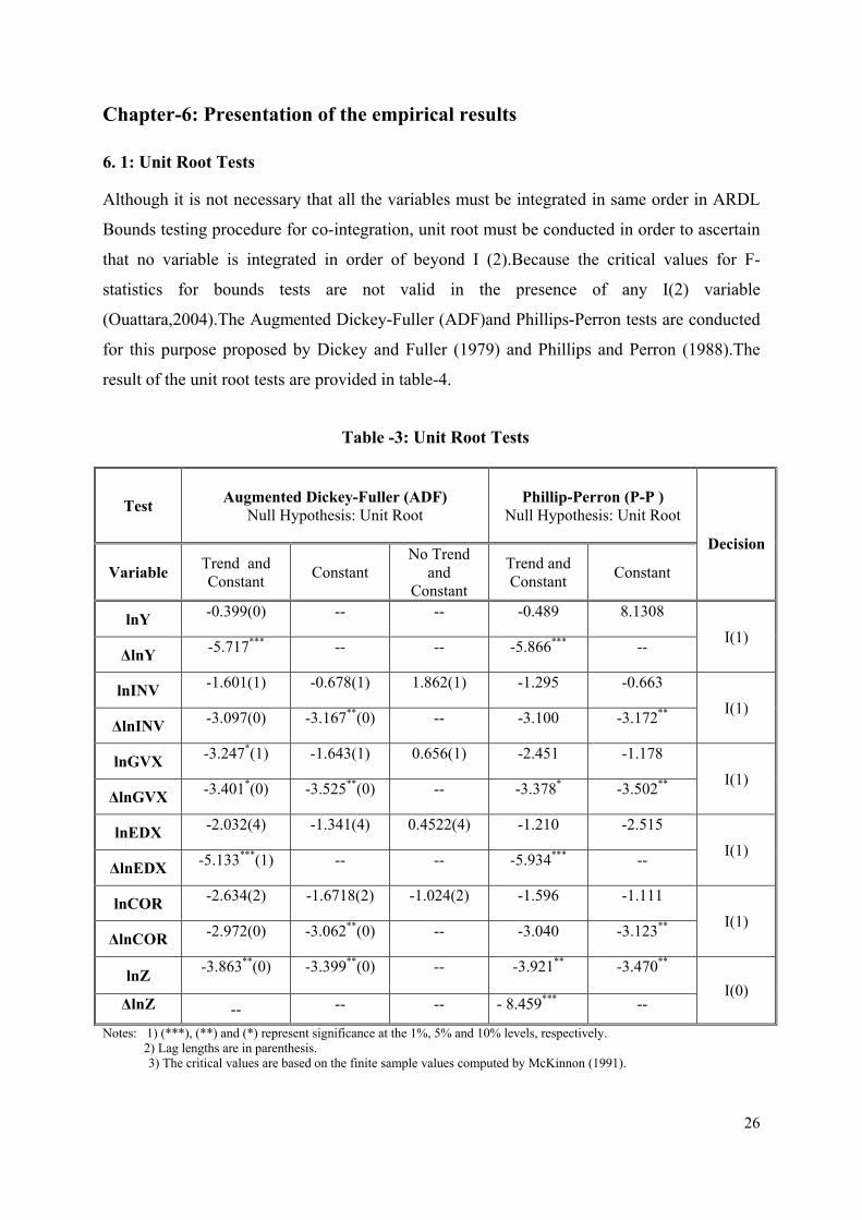
6. 1: Unit Root Tests

Although it is not necessary that all the variables must be integrated in same order in ARDL

Bounds testing procedure for co-integration, unit root must be conducted in order to ascertain

that no variable is integrated in order of beyond I (2).Because the critical values for F-

statistics for bounds tests are not valid in the presence of any I(2) variable

(Ouattara,2004).The Augmented Dickey-Fuller (ADF)and Phillips-Perron tests are conducted

for this purpose proposed by Dickey and Fuller (1979) and Phillips and Perron (1988).The

result of the unit root tests are provided in table-4.

Notes: 1) (***), (**) and (*) represent significance at the 1%, 5% and 10% levels, respectively. 2) Lag lengths are in parenthesis.

3) The critical values are based on the finite sample values computed by McKinnon (1991).

Table -3: Unit Root Tests

Test

Augmented Dickey-Fuller (ADF)

Null Hypothesis: Unit Root

Phillip-Perron (P-P )

Null Hypothesis: Unit Root

Decision

Variable Trend and Constant

Constant

No Trend and

Constant

Trend and Constant

Constant

lnY -0.399(0) -- -- -0.489 8.1308

I(1) ΔlnY

-5.717*** -- -- -5.866*** --

lnINV -1.601(1) -0.678(1) 1.862(1) -1.295 -0.663

I(1)

ΔlnINV -3.097(0) -3.167**(0) -- -3.100 -3.172**

lnGVX -3.247*(1) -1.643(1) 0.656(1) -2.451 -1.178

I(1) ΔlnGVX

-3.401*(0) -3.525**(0) -- -3.378* -3.502**

lnEDX -2.032(4) -1.341(4) 0.4522(4) -1.210 -2.515

I(1) ΔlnEDX

-5.133***(1) -- -- -5.934*** --

lnCOR -2.634(2) -1.6718(2) -1.024(2) -1.596 -1.111

I(1) ΔlnCOR

-2.972(0) -3.062**(0) -- -3.040 -3.123**

lnZ -3.863**(0)

-3.399**(0) -- -3.921** -3.470**

I(0) ΔlnZ -- -- -- - 8.459*** --

27  

The last column of the table reports the order of integration. The null hypothesis of existence

of unit root in both tests is tested against alternative hypothesis of no unit root.I draw

conclusion about the order of integration whether the series has both trend and constant and

only constant or no constant and trend. I have chosen 5% significant level to test the null

hypotheses in each case. The result indicates that all variables expect lnZ are non-stationary at

their levels but stationary when 1st difference is taken in each test. The series lnY is non-

stationary with trend and constant but it becomes stationary at 1 % level after taking the 1st

difference. lnEDX is also stationary at 1% level at it is 1st difference. According to ADF test

lnZ is I (0) but I (1) in PP test. As none of the selected series is beyond (1) according to two

unit root tests results, I can confidently apply Bounds test to examine co-integration among

variables.

6. 2: Results of Bounds Test for Co-integration

In the first stage of Bounds test, I conduct OLS regression for the base model as well as the

model with corruption. To obtain parsimonious specification I have adopted “General-to-

Specific Modeling” approach guided by short data span .In this case, I have chosen 2(two) as

maximum order of legs as the observations are annual suggested by Pesaran and Shin (1999)

and Narayan (2004).Here, it must be noted that visual inspection of all the series indicates that

there may be one structural break in the series of government final consumption expenditure

in 1993. In order to be certain, I have applied Quandt likelihood ratio16 (QLR) test for

detecting the structural break in the models. The result of this test identifies that there is in

fact a structural break in 1993.Therefore, I put a dummy variable “D1” for this period in each

model when the OLS regression is performed. To work with general-to-specific modeling

procedure, I have eliminated the insignificant lags except for the level variables and intercept.

The benefit of this approach is that it ensures the assumption of no serial correlation as

emphasized by Pesaran et.al (2001) and normality is not violated. I have used Akaike

Information Criterion (AIC) to determine the optimal number of lags to be included in the

unconditional ARDL-ECMs. Thus the order of selected ARDL models are of (1, 1, 1, 0, 1)

and (1, 1, 1, 0, 1, 0) for the base model and model with corruption respectively.

                                                            16

Detail is available in the article “Tests for Parameter Instability and Structural Change With Unknown Change

Point” by Donald W. K. Andrews(1993)

28  

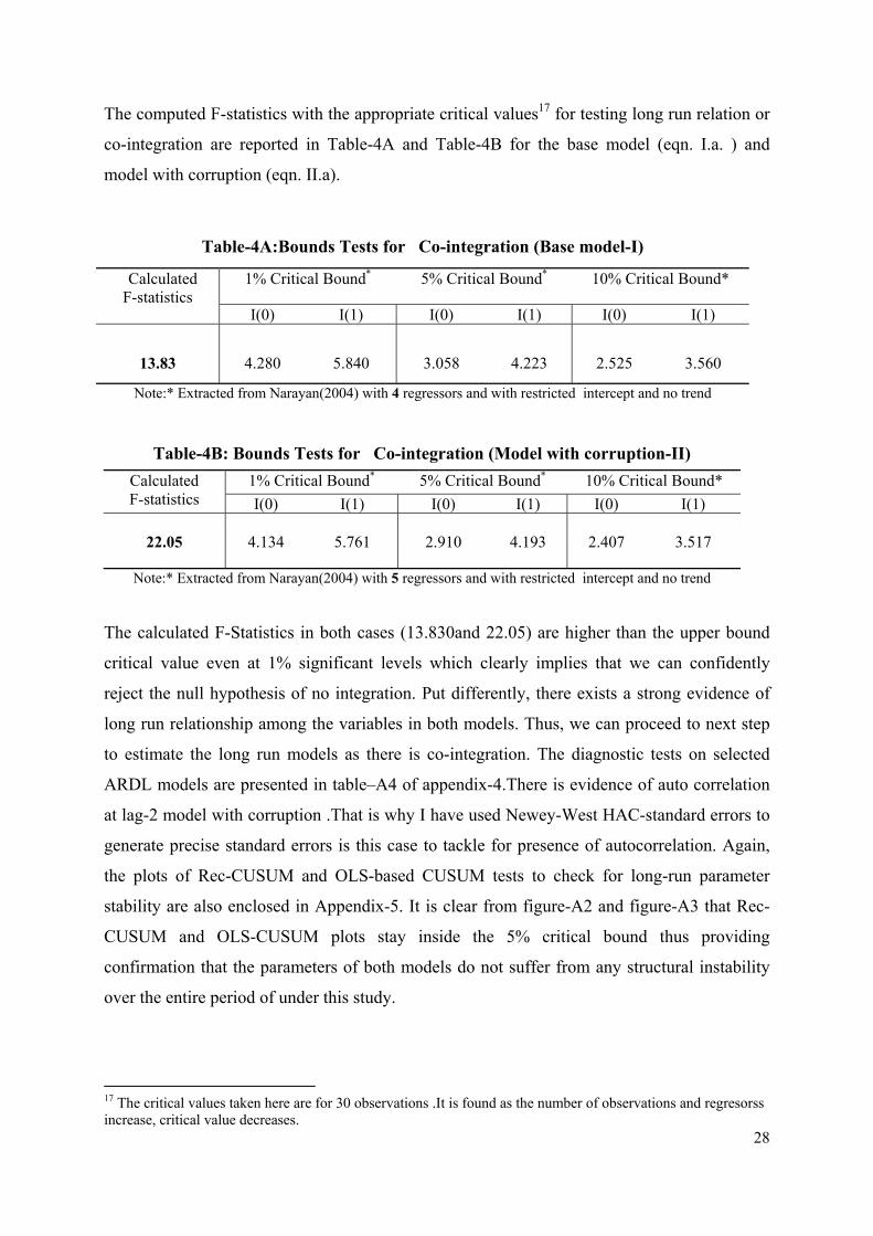
The computed F-statistics with the appropriate critical values17 for testing long run relation or

co-integration are reported in Table-4A and Table-4B for the base model (eqn. I.a. ) and

model with corruption (eqn. II.a).

The calculated F-Statistics in both cases (13.830and 22.05) are higher than the upper bound

critical value even at 1% significant levels which clearly implies that we can confidently

reject the null hypothesis of no integration. Put differently, there exists a strong evidence of

long run relationship among the variables in both models. Thus, we can proceed to next step

to estimate the long run models as there is co-integration. The diagnostic tests on selected

ARDL models are presented in table–A4 of appendix-4.There is evidence of auto correlation

at lag-2 model with corruption .That is why I have used Newey-West HAC-standard errors to

generate precise standard errors is this case to tackle for presence of autocorrelation. Again,

the plots of Rec-CUSUM and OLS-based CUSUM tests to check for long-run parameter

stability are also enclosed in Appendix-5. It is clear from figure-A2 and figure-A3 that Rec-

CUSUM and OLS-CUSUM plots stay inside the 5% critical bound thus providing

confirmation that the parameters of both models do not suffer from any structural instability

over the entire period of under this study.

                                                            17 The critical values taken here are for 30 observations .It is found as the number of observations and regresorss increase, critical value decreases.

Table-4A:Bounds Tests for Co-integration (Base model-I)

Calculated F-statistics

1% Critical Bound* 5% Critical Bound* 10% Critical Bound*

I(0) I(1) I(0) I(1) I(0) I(1)

13.83 4.280 5.840 3.058 4.223 2.525 3.560

Table-4B: Bounds Tests for Co-integration (Model with corruption-II)

Calculated F-statistics

1% Critical Bound* 5% Critical Bound* 10% Critical Bound*

I(0) I(1) I(0) I(1) I(0) I(1)

22.05 4.134 5.761 2.910 4.193 2.407 3.517

Note:* Extracted from Narayan(2004) with 5 regressors and with restricted intercept and no trend

Note:* Extracted from Narayan(2004) with 4 regressors and with restricted intercept and no trend

29  

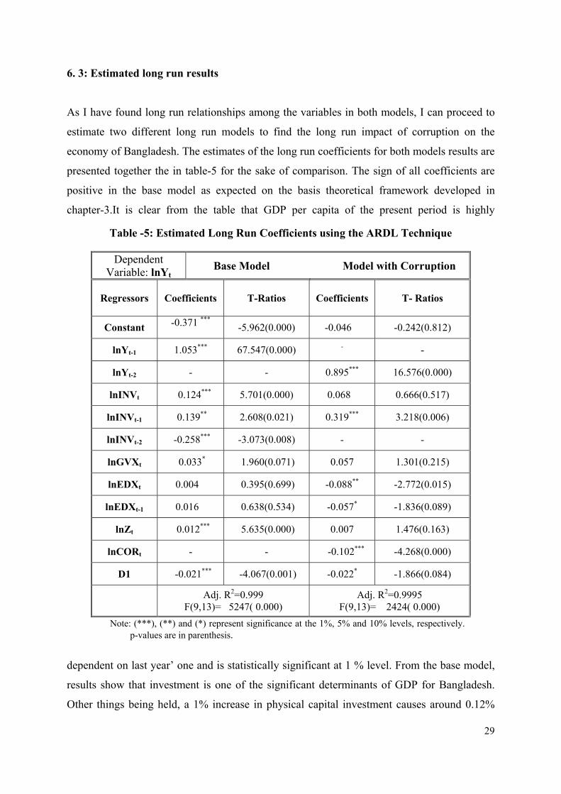
6. 3: Estimated long run results

As I have found long run relationships among the variables in both models, I can proceed to

estimate two different long run models to find the long run impact of corruption on the

economy of Bangladesh. The estimates of the long run coefficients for both models results are

presented together the in table-5 for the sake of comparison. The sign of all coefficients are

positive in the base model as expected on the basis theoretical framework developed in

chapter-3.It is clear from the table that GDP per capita of the present period is highly

dependent on last year’ one and is statistically significant at 1 % level. From the base model,

results show that investment is one of the significant determinants of GDP for Bangladesh.

Other things being held, a 1% increase in physical capital investment causes around 0.12%

Table -5: Estimated Long Run Coefficients using the ARDL Technique

Dependent Variable: lnYt

Base Model Model with Corruption

Regressors

Coefficients

T-Ratios Coefficients T- Ratios

Constant -0.371 ***

-5.962(0.000) -0.046 -0.242(0.812)

lnYt-1 1.053*** 67.547(0.000) - -

lnYt-2 - - 0.895*** 16.576(0.000)

lnINVt 0.124*** 5.701(0.000) 0.068 0.666(0.517)

lnINVt-1 0.139** 2.608(0.021) 0.319*** 3.218(0.006)

lnINVt-2 -0.258*** -3.073(0.008) - -

lnGVXt 0.033* 1.960(0.071) 0.057 1.301(0.215)

lnEDXt 0.004 0.395(0.699) -0.088** -2.772(0.015)

lnEDXt-1 0.016 0.638(0.534) -0.057* -1.836(0.089)

lnZt 0.012*** 5.635(0.000) 0.007 1.476(0.163)

lnCORt - - -0.102*** -4.268(0.000)

D1 -0.021*** -4.067(0.001) -0.022* -1.866(0.084)

Adj. R2=0.999

F(9,13)= 5247( 0.000) Adj. R2=0.9995

F(9,13)= 2424( 0.000)

Note: (***), (**) and (*) represent significance at the 1%, 5% and 10% levels, respectively.

p-values are in parenthesis.

30  

increment in per capita real GDP. lnGVX is significant at 10% level and a 1% rise in GVX

leads to around 0.3% increase in per capita GDP. It reveals that government expenditure in

other words public sector is not contributing to economic growth in Bangladesh as much as

expected in a developing county. Public expenditure on education (lnEDX) does not have a

significant impact on GDP in statistical terms and its magnitude is also small (0.004). The

estimate of the accumulated term lnZ is significant at 1% level but effect on the economy is

very low (0.012). Now I am going to analyze the results of the extended model with

corruption. After adding corruption as an independent variable in the regression analysis,

corruption (lnCOR) is found to be highly significant (at 1% level) and its effect on real GDP

per capita of Bangladesh during 1984-2008 in negative. It shows the direct impact of

corruption in the economy in the long run. According to our results, real per capita GDP in

Bangladesh reduces by 0.10%in the long run if there is a1% increase in the level of corruption

other thing being held constant. This result is similar to the findings of cross sectional study of

Mauro (1995), Rahman et.al (2000) and Dreher and Herzfel (2005). Based on the above

results, we can say that real GDP per capita in Bangladesh would be 508.20 US$ instead of

462.12 US$ in 2008 if it could reduce its level of corruption by 1%.

Now let us move to the discussion on how corruption is affecting the economy through

different mechanisms i.e. indirect affect described in the theoretical chapter. Table-5 reports

that coefficient of physical capital investment (lnINV) has become insignificant at the

presence of corruption and its magnitude is also reduced to 0.068. It implies that corruption

has substantial negative consequence on investment of Bangladesh. Previous cross sectional

empirical studies have also found similar result. On the other hand, the size of the coefficient

for government final consumption expenditure (lnGVX) or public sector investment has

increased but it insignificant now. In this regard, we can say that public sector investment has

increased but it does have not significant contribution to the economic growth of Bangladesh.

Earlier studies such as Gupta, Mello and Sharan(2001), Tanzi and Davoodi (1997) Mauro

(1998) have got this kind of result in cross country analysis. In developing countries, there are

many opportunities of corruption in public sector. For example, government official and

politicians can take bribe by importing unnecessary modern technological equipments, which

are not appropriate in the current stage of development. My findings also indicate that

corruption has negative impact on human capital investment. The result shows that public

sector education expenditure has negative influence on per capita GDP at presence of

corruption in Bangladesh.

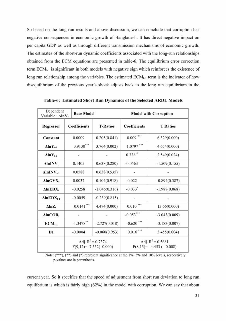
31  

So based on the long run results and above discussion, we can conclude that corruption has

negative consequences in economic growth of Bangladesh. It has direct negative impact on

per capita GDP as well as through different transmission mechanisms of economic growth.

The estimates of the short-run dynamic coefficients associated with the long-run relationships

obtained from the ECM equations are presented in table-6. The equilibrium error correction

term ECMt-1 is significant in both models with negative sign which reinforces the existence of

long run relationship among the variables. The estimated ECMt-1 term is the indicator of how

disequilibrium of the previous year’s shock adjusts back to the long run equilibrium in the

current year. So it specifies that the speed of adjustment from short run deviation to long run

equilibrium is which is fairly high (62%) in the model with corruption. We can say that about

Table-6: Estimated Short Run Dynamics of the Selected ARDL Models

Dependent Variable : ΔlnYt

Base Model Model with Corruption

Regressor

Coefficients

T-Ratios Coefficients T Ratios

Constant 0.0009 0.205(0.841) 0.009**** 6.329(0.000)

ΔlnYt-1 0.9130*** 3.764(0.002) 1.0797 *** 4.654(0.000)

ΔlnYt-2 - - 0.338** 2.549(0.024)

ΔlnINVt 0.1405 0.638(0.280) -0.0563 -1.509(0.155)

ΔlnINVt-1 0.0588 0.638(0.535) - -

ΔlnGVXt 0.0037 0.104(0.918) -0.022 -0.894(0.387)

ΔlnEDXt -0.0258 -1.046(0.316) -0.033* -1.988(0.068)

ΔlnEDXt-1 -0.0059 -0.239(0.815) - -

ΔlnZt 0.0141*** 4.474(0.000) 0.010 *** 13.66(0.000)

ΔlnCORt - - -0.053*** -3.043(0.009)

ECMt-1 -1.3478** -2.727(0.018) -0.620 *** -3.183(0.007)

D1 -0.0004 -0.060(0.953) 0.016 *** 3.455(0.004)

Adj. R2 = 0.7374

F(9,12)= 7.552( 0.000) Adj. R2 = 0.5681

F(8,13)= 4.453 ( 0.008)

Note: (***), (**) and (*) represent significance at the 1%, 5% and 10% levels, respectively.

p-values are in parenthesis.

32  

62% of imbalance from the preceding year’s shock converges back to the long-run

equilibrium in the current year. The results of the diagnostic tests for long run models as well

as error correction models are reported in table-A5 and table-A6 respectively in appendix-4.

Chapter-7: Concluding Remarks

Corruption has become rampant almost in every sphere of life in Bangladesh. The country is

listed as one of the most corrupt counties in the world in various rankings of corruption. It is

widely discussed that corruption is hurting economic progress of the country to a large extent.

News Scan Analysis of Transparency International Bangladesh (2002) reports that about

1.85% of the GDP had been lost because of corruption in the fiscal year of 1999-2000.

The main objective of this thesis is to empirically investigate the impact of corruption on the

economic development of Bangladesh using annual time series data for the period of 1984-

2008. According to my knowledge, this is the first attempt to apply a multivariate approach to

examine the relationship between GDP per capita and corruption for Bangladesh using time

series data.

With a view to achieving the aim of the thesis, I have extended the Solow model of economic

growth to include public sector and human capital and then reformulated this augmented

model incorporating corruption in a specific functional form to decompose the direct and

indirect consequences of corruption on income per capita. Based on the priori assumption of

negative consequences of corruption, this model entails how corruption directly affects per

capita income through total factor productivity channel as well as indirectly via physical

capital, public sector and human capital channel. Then I have tested the long run relationship

between corruption and real GDP per capita for that time span using ARDL Bounds method

for co-integration using International Country Risk Guide (ICRG) corruption index as a proxy

to measure the level corruption in Bangladesh. The results of co-integration test confirms that

there is a long run relation among corruption, GDP per capita and other determinants of GDP

over this period. The long run estimates indicate that corruption has direct negative impact on

per capita GDP i.e. economic development of Bangladesh. It shows that a 1% increase in the

33  

level of corruption during this period has resulted in about 10% reduction in per capita GDP

of Bangladesh. It means that corruption is affecting the economic growth of Bangladesh

adversely. In other words that Bangladesh could achieve faster economic development if it

could curb widespread corruption. This finding is similar to the results of Mauro (1995),

Rahman, Kisunko and Kapoor (2000) and Dreher and Herzfel (2005) but differs in magnitude

as these studies are based on average of cross sectional data for different time period. Results

from my study also suggest that corruption has strong negative impact on physical capital

investment and human development in Bangladesh. The findings imply that corruption has

increased public sector investment but it does not have significant contribution to economic

growth of Bangladesh in the presence of high level of corruption.

The main limitation of my study is the short time span that the study considers and annual

data. The reason behind that is the unavailability of the data on measurement of corruption for

longer time period. Besides trade and remittances from abroad have significant contributions

in economic growth of Bangladesh in recent years, a fact that has not been considered in this

study. Future researches may get results that are more robust after the inclusion of these

determinants of GDP using data for longer periods. However, it will not probably alter the

conclusion drawn from my time series analysis that corruption has strong and significant

retarding consequences on economic development of Bangladesh.

34  

References:

Akçay, S. (2006): “Corruption and Human Development”. Cato Journal,26, No. 1

Aidt, T. S. (2003): “Economic Analysis of Corruption: A Survey”. Economic Journal, 113 (491), 632-652.

Arrow K. and Kurz. M (1970): “Public investment, the rate of return and optimal fiscal

policy”. The Johns Hopkins University Press, Baltimore. Banerjee, A., Dolado, J. J., Galbraith, J. W., and. Hendry D.F. (1993): “Co-integration, Error-

correction, and the Econometric Analysis of Non-stationary Data” Oxford

University Press, Oxford. Barreto, R. A. (2000): “Endogenous Corruption in a Neoclassical Growth Model”. European

Economic Review, 44(1), 35-60. Barro, R. J. (1990): "Government Spending in a Simple Model of Endogenous Growth".

Journal of Political Economy, 98(5:2), S103-S125. Barro, R.J., (1991): “Economic growth in a cross section of countries”. Quarterly Journal of

Economics, 106(2), 407-443. Barro, R. J. (1996):“Determinants of Economic Growth: A Cross-Country Empirical Study”.

NBER Working Paper, No. 5698. Brown, R.L., Durbin, J. and Evans, J.M (1975):'Techniques for Testing the Consitency of

Regression Relations Over Time', Journal of the Royal Statistical Society, 37, 149-92.

Brunetti, A. (1997): “Political variables in cross-country growth analysis”. Journal of

Economic Surveys, 11(2), 163-190. Campos, J. E., Lien, D. and Pradhan, S. (1999): “The Impact of Corruption on Investment:

Predictability Matters”. World Development, 27 (6), 1059-1067. Campos, J.E. (2001):“Corruption: the boom and bust of East Asia”. Quezon City: Ateneo de

Manila University Press. Del Monte, A. and E. Papagni (2001): “Public expenditure, corruption, and economic growth:

the case of Italy”. European Journal of Political Economy17, 1–16.

Dreher, .A and Herzfel, T(2005):“The Economic Costs of Corruption: A Survey and New

Evidence” Unpublished available at http://mpra.ub.uni-muenchen.de/23578/.

Dickey, D. A. and Fuller W. A. (1981): “Likelihood Ratio Statistics for Autoregressive Time

Series with a Unit Root,” Econometrica, 49, 1057-1072.

35  

Ehrlich,I. and Lui, F. T. (1999): “Bureaucratic Corruption and Endogenous Economic

Growth”. Journal of Political Economy,107(6:2), S270-S293.

Enders, W. (2004): “Applied Econometric Time Series” 2nd

Edition

Engle, R. and C. Granger (1987) “Cointegration and Error Correction Representation: Estimation and Testing”. Econometrica 55, 251-276.

Groningen Growth and Development Centre (GGDC). Faculty of Economics, University of Groningen, Netherlands: GGDC:www.ggdc.net

Gupta, S., De Mello, L. and Sharan, R. (2001): “Corruption and Military Spending”.

European Journal of Political Economy, 17 (4), 749-777

Gupta , S., Davoodi, H. R. and Tiongson, E. R. (2002): “Corruption and the Provision of

Health Care and Education Services”,Governance, Corruption, & Economic

Performance, International Monetary Fund, Publication Services, Washington,

D.C., 254-279

Huntington, S. P. (1968):“Political Order in Changing Societies”. New Haven: Yale

University Press. Johansen, S. and K. Juselius (1990) Maximum Likelihood Estimation and Inference on

Cointegration–with Application to the Demand for Money, Oxford Bulletin of

Economics and Statistics 52, 169-210. Khan, M. M. (1998): “Political and Administrative Corruption: Concepts, Comparative

Experiences and Bangladesh Case”. A paper prepared for Transparency

International Bangladesh (TIB), Dhaka. Kiltgaard, R. (1998): “International cooperation against corruption”, IMF/World Bank,

Finance and Development, 35(1), 3. Knack, S., and Keefer, P. (1995):“Institutions and Economic Performance: Cross Country

Tests Using Alternative Institutional Measures”, Economics and Politics, 7, 207-227

Lambsdorff, J. G. (2003): “How corruption affects productivity”. Kyklos 56(4), 457–474. Lambsdorff, J. G. (1999):“Corruption in Empirical Research - A Review.” Transparency

International Working Paper

Leff, N. (1964):“Economic Development through Bureaucratic Corruption”. American

Behavioural Scientist, 8, 8-14. Levine, R. and D. Renelt, (1992):“A sensitivity analysis of cross-country growth regressions”.

American Economic Review, 82, 942-963.

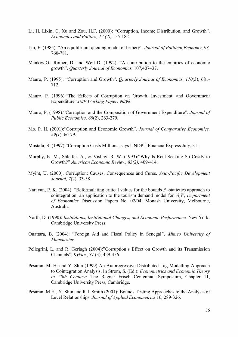
36  

Li, H. Lixin, C. Xu and Zou, H.F. (2000): “Corruption, Income Distribution, and Growth”. Economics and Politics, 12 (2), 155-182

Lui, F. (1985): “An equilibrium queuing model of bribery”, Journal of Political Economy, 93,

760-781.

Mankiw,G., Romer, D. and Weil D. (1992): “A contribution to the empirics of economic growth”. Quarterly Journal of Economics, 107,407–37.

Mauro, P. (1995): “Corruption and Growth”. Quarterly Journal of Economics, 110(3), 681-

712. Mauro, P. (1996):“The Effects of Corruption on Growth, Investment, and Government

Expenditure”.IMF Working Paper, 96/98. Mauro, P. (1998):“Corruption and the Composition of Government Expenditure”. Journal of

Public Economics, 69(2), 263-279. Mo, P. H. (2001):“Corruption and Economic Growth”. Journal of Comparative Economics,

29(1), 66-79. Mustafa, S. (1997):“Corruption Costs Millions, says UNDP”, FinancialExpress July, 31. Murphy, K. M., Shleifer, A., & Vishny, R. W. (1993):“Why Is Rent-Seeking So Costly to

Growth?” American Economic Review, 83(2), 409-414. Myint, U. (2000). Corruption: Causes, Consequences and Cures. Asia-Pacific Development

Journal, 7(2), 33-58. Narayan, P. K. (2004): “Reformulating critical values for the bounds F -statictics approach to

cointegration: an application to the tourism demand model for Fiji”, Department

of Economics Discussion Papers No. 02/04, Monash University, Melbourne, Australia

North, D. (1990): Institutions, Institutional Changes, and Economic Performance. New York:

Cambridge University Press Ouattara, B. (2004): “Foreign Aid and Fiscal Policy in Senegal”. Mimeo University of

Manchester.

Pellegrini, L. and R. Gerlagh (2004):”Corruption’s Effect on Growth and its Transmission Channels”, Kyklos, 57 (3), 429-456.

Pesaran, M. H. and Y. Shin (1999) An Autoregressive Distributed Lag Modelling Approach

to Cointegration Analysis, In Strom, S. (Ed.): Econometrics and Economic Theory

in 20th Century: The Ragnar Frisch Centennial Symposium, Chapter 11, Cambridge University Press, Cambridge.

Pesaran, M.H., Y. Shin and R.J. Smith (2001): Bounds Testing Approaches to the Analysis of Level Relationships. Journal of Applied Econometrics 16, 289-326.

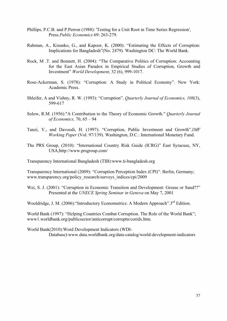
37  

Phillips, P.C.B. and P.Perron (1988): 'Testing for a Unit Root in Time Series Regression', Press.Public Economics 69: 263-279.

Rahman, A., Kisunko, G., and Kapoor, K. (2000): “Estimating the Effects of Corruption:

Implications for Bangladesh”(No. 2479). Washington DC: The World Bank. Rock, M .T. and Bonnett, H. (2004): “The Comparative Politics of Corruption: Accounting

for the East Asian Paradox in Empirical Studies of Corruption, Growth and Investment” World Development, 32 (6), 999-1017.

Rose-Ackerman, S. (1978): “Corruption: A Study in Political Economy”. New York:

Academic Press. Shleifer, A and Vishny, R. W. (1993): “Corruption”. Quarterly Journal of Economics, 108(3),

599-617 Solow, R.M. (1956):"A Contribution to the Theory of Economic Growth." Quarterly Journal

of Economics, 70, 65 – 94 Tanzi, V., and Davoodi, H. (1997): “Corruption, Public Investment and Growth”.IMF

Working Paper (Vol. 97/139). Washington, D.C.: International Monetary Fund. The PRS Group, (2010): “International Country Risk Guide (ICRG)” East Syracuse, NY,

USA;http://www.prsgroup.com/ Transparency International Bangladesh (TIB):www.ti-bangladesh.org Transparency International (2009): “Corruption Perception Index (CPI)”. Berlin, Germany; www.transparency.org/policy_research/surveys_indices/cpi/2009 Wei, S. J. (2001): “Corruption in Economic Transition and Development: Grease or Sand??”

Presented at the UNECE Spring Seminar in Geneva on May 7, 2001 Wooldridge, J. M. (2006):“Introductory Econometrics: A Modern Approach”.3rd Edition. World Bank (1997): “Helping Countries Combat Corruption. The Role of the World Bank”; www1.worldbank.org/publicsector/anticorrupt/corruptn/coridx.htm.

World Bank(2010):Word Development Indicators (WDI-Database):www.data.worldbank.org/data-catalog/world-development-indicators

 

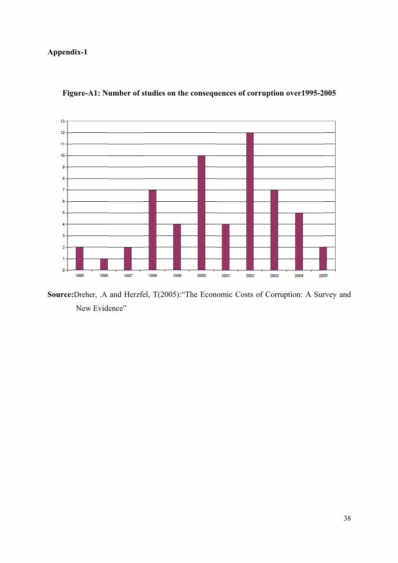
Append

Fig

Source:

dix-1

gure-A1: N

:Dreher, .A

New Evid

umber of s

and Herzfe

dence”

studies on t

el, T(2005):

the consequ

:“The Econ

uences of co

nomic Costs

orruption o

s of Corrup

over1995-2

tion: A Sur

38 

005

rvey and

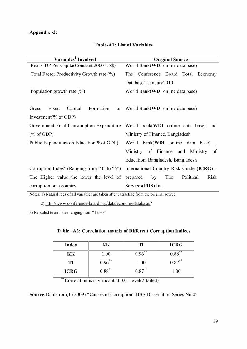
39  

Appendix -2:

Table-A1: List of Variables

Notes: 1) Natural logs of all variables are taken after extracting from the original source.

2) http://www.conference-board.org/data/economydatabase/"

3) Rescaled to an index ranging from “1 to 0”

Table –A2: Correlation matrix of Different Corruption Indices

Source:Dahlstrom,T.(2009):“Causes of Corruption” JIBS Dissertation Series No.05

Variables1 Involved

Original Source

Real GDP Per Capita(Constant 2000 US$) World Bank(WDI online data base)

Total Factor Productivity Growth rate (%) The Conference Board Total Economy

Database2, January2010

Population growth rate (%)

World Bank(WDI online data base)

Gross Fixed Capital Formation or

Investment(% of GDP)

World Bank(WDI online data base)

Government Final Consumption Expenditure

(% of GDP)

World bank(WDI online data base) and

Ministry of Finance, Bangladesh

Public Expenditure on Education(%of GDP) World bank(WDI online data base) ,

Ministry of Finance and Ministry of

Education, Bangladesh, Bangladesh

Corruption Index3 (Ranging from “0” to “6”)

The Higher value the lower the level of

corruption on a country.

International Country Risk Guide (ICRG) -

prepared by The Political Risk

Services(PRS) Inc.

Index KK TI ICRG

KK 1.00 0.96** 0.88**

TI 0.96** 1.00 0.87**

ICRG 0.88** 0.87** 1.00

** Correlation is significant at 0.01 level(2-tailed)

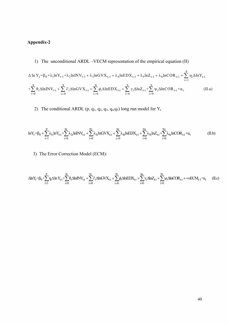
40  

Appendix-2

1) The unconditional ARDL –VECM representation of the empirical equation (II)

p

t 0 1 t-1 2 t-1 3 t-1 4 t-1 5 t-1 6 t-1 i t-ii=1

q q q q q

i t-i t-i t-i i t-i i t-i ti=0 i 0 i 0 i=0 i=0

ln Y =β +λ lnY +λ lnINV λ lnGVX λ lnEDX λ lnZ λ lnCOR η ΔlnY

+ θ ΔlnINV lnGVX lnEDX γ ΔlnZ + ψ ΔlnCOR +u (II.a)i i

2) The conditional ARDL (p, q1, q2, q3, q4,q5) long run model for Yt

3 51 2 4q qq q qp

t 0 1i t-i 2i t-i 3i t-i 4i t-i 5i t-i 6i t-i ti=1 i=0 i=0 i 0 i=0 i=0

lnY =β λ lnY + λ lnINV λ lnGVX λ lnEDX λ lnZ + λ lnCOR +u (II.b)

3) The Error Correction Model (ECM):

3 51 2 4q qq q qp

t 0 i t-i i t-i t-i t-i i t-i i t-i t-1 ti=1 i=0 i 0 i 0 i=0 i=0

lnY =β + η lnY + θΔlnINV lnGVX lnEDX γΔlnZ ψΔlnCOR υECM +u (II.c)i i

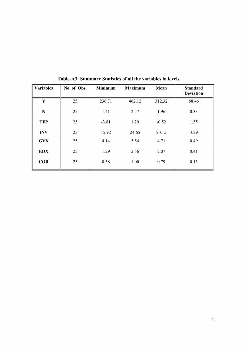
41  

Table-A3: Summary Statistics of all the variables in levels

Variables No. of Obs. Minimum Maximum Mean Standard

Deviation

Y 25 236.71 462.12

312.32 68.46

N 25 1.41 2.57

1.96 0.33

TFP 25 -3.81 1.29

-0.52 1.55

INV 25 15.92 24.65 20.15 3.29

GVX 25 4.14 5.54

4.71 0.49

EDX 25 1.29 2.56

2.07 0.41

COR 25 0.58 1.00

0.79 0.15

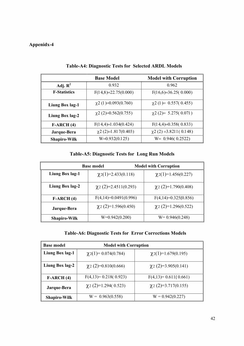
42  

Appenidx-4

Table-A4: Diagnostic Tests for Selected ARDL Models

Base Model Model with Corruption

Adj. R2

F-Statistics

F F

Liung Box lag-1

Liung Box lag-2

F-ARCH (4) F F

Jarque-Bera

Shapiro-Wilk W W

Table-A5: Diagnostic Tests for Long Run Models

Base model Model with Corruption

Liung Box lag-1

2(1)=2.433(0.118) 2(1)=1.456(0.227)

Liung Box lag-2

2 (2)=2.4511(0.293)

2 (2)=1.790(0.408)

F-ARCH (4) F(4,14)=0.0491(0.996) F(4,14)=0.325(0.856)

Jarque-Bera 2 (2)=1.596(0.450) 2 (2)=1.296(0.522)

Shapiro-Wilk W=0.942(0.200) W= 0.946(0.248)

Table-A6: Diagnostic Tests for Error Corrections Models

Base model Model with Corruption

Liung Box lag-1

2(1)= 0.074(0.784) 2(1)=1.679(0.195)

Liung Box lag-2

2 (2)=0.810(0.666)

2 (2)=3.905(0.141)

F-ARCH (4) F(4,13)= 0.218( 0.923) F(4,13)= 0.611( 0.661)

Jarque-Bera 2 (2)=1.294( 0.523) 2 (2)=3.717(0.155)

Shapiro-Wilk W = 0.963(0.558) W = 0.942(0.227)

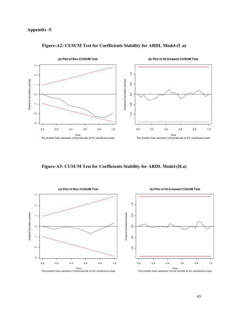
43  

Appendix -5

Figure-A2: CUSUM Test for Coefficients Stability for ARDL Model-(I .a)

Figure-A3: CUSUM Test for Coefficients Stability for ARDL Model-(II.a)

(a) Plot of Rec-CUSUM Test

The straight lines represent critical bounds at 5% significance level

Time

Em

piric

al fluctu

ation p

rocess

0.0 0.2 0.4 0.6 0.8 1.0

-3-2

-10

12

3

(b) Plot of OLS-based CUSUM Test

The straight lines represent critical bounds at 5% significance level

Time

Em

piric

al fluctu

ation p

rocess

0.0 0.2 0.4 0.6 0.8 1.0-1

.0-0

.50.0

0.5

1.0

(a) Plot of Rec-CUSUM Test

The straight lines represent critical bounds at 5% significance level

Time

Em

piric

al fluctu

ation p

rocess

0.0 0.2 0.4 0.6 0.8 1.0

-3-2

-10

12

3

(b) Plot of OLS-based CUSUM Test

The straight lines represent critical bounds at 5% significance level

Time

Em

piric

al fluctu

ation p

rocess

0.0 0.2 0.4 0.6 0.8 1.0

-1.0

-0.5

0.0

0.5

1.0