The Impact of Hedging on Stock Returns and Firm

Value:

New Evidence from Canadian Oil and Gas Companies

Chang Dan, Hong Gu and Kuan Xu∗

∗Chang Dan, Financial Analyst, Chang Jiang Securities, Wuhan, China. Hong Gu, Associate Pro-fessor of Statistics, Department of Mathematics and Statistics, Dalhousie University, Halifax, Canada.Kuan Xu, Professor of Economics, Department of Economics, Dalhousie University, Halifax, Canada.Correspondence: Kuan Xu, Department of Economics, Dalhousie University, Halifax, Nova Scotia,Canada B3H 3J5. E-mail: kxu@is.dal.ca. We thank Shamsud Chowdhury, Iraj Fooladi, Greg Hebb,Yanbo Jin, Barry Lesser, Maria Pacurar, John Rumsey, Oumar Sy and participants of the School ofBusiness and the Department of Economics Seminars at Dalhousie University for their helpful commentson the earlier draft of this paper. Remaining errors are, of course, the responsibility of authors.

1

The Impact of Hedging on Stock Returns and Firm

Value:

New Evidence from Canadian Oil and Gas

Companies

Abstract

In this paper we analyze (a) the impact of hedging activities on the relationships

between oil and gas prices/reserves and stock returns and (b) the role of hedging on

firm value among large Canadian oil and gas companies. Differing from the existing

literature this research attempts to explore possible nonlinear impact of hedging

activities, which may not be fully revealed in the traditional linear framework. By

using generalized additive models, we find that factors that affect stock returns

and firm value are indeed nonlinear. The large Canadian oil and gas firms are able

to hedge against downside risk induced by unfavorable oil and gas price changes.

But gas hedging appears to be more effective than oil hedging when downside risk

presents. In addition, oil reserves tend to have a positive (negative) impact on

stock returns when the oil prices are increasing (decreasing). Finally, hedging, in

particular hedging for gas, together with profitability, leverage and reserves, has a

significant impact on firm value.

Keywords: hedging, risk management, oil and gas, equity returns, Tobin’s Q ratio,

generalized additive model, semi-parametric model, nonlinearity

JEL classification: G100, C100

2

1 Introduction

According to the Modigliani-Miller theorem, in a perfect financial market, hedging would

add no value to the firm when there is no asymmetric information, taxes, or transaction

costs. However, in the real world, this conclusion may not hold because the assumptions

on which the theorem is based are generally violated.

Maximizing shareholder value is one of the main aims of the corporate management.

Maximizing shareholder value means maintaining and increasing the cash flow of the

corporation over time. The literature on hedging notes that there are three main moti-

vations for firms to hedge. First, hedging is used to reduce financial distress and avoid

underinvestment [see, for example, Smith and Stulz (1985), Mayers and Smith (1990),

Stulz (1990), Froot et al. (1993), Allayannis and Mozumdar (2000), and Adam (2002)].

Second, hedging is used to reduce expected tax costs [see, for example, Smith and Stulz

(1985), Graham and Smith (1999), and Graham and Rogers (2002)]. Third, hedging can

alleviate the manager’s personal risk exposure [see, for example, Stulz (1984), Smith and

Stulz (1985), DeMarzo and Duffie (1995), Tufano (1996), Whidbee and Wohar (1999),

and Dionne and Triki (2005)].

The literature on the effectiveness of hedging has focused primarily on the hedging

activities in the financial and commodity risk management. For financial risk manage-

ment, Jorion (1990) illustrates that the foreign currency beta of the U.S. multinational

companies is close to zero, meaning hedging on foreign currency does not influence firm

value at all. Geczy et al. (1997) analyze foreign currency derivatives of Fortune 500

companies and find that hedging for foreign currency risk is more difficult to evaluate in

multinational companies because the net impact of hedging can be distorted by many

other factors such as foreign sales, foreign-denominated debts, foreign taxes, etc. On the

other hand, Gagnon et al. (1998) employ constructed currency portfolios to show that

dynamic hedging strategies can indeed reduce risk. Allayannis and Weston (2001) di-

3

rectly study the relationship between foreign currency hedging and firm value measured

by Tobin’s Q ratio of the U.S. non-financial firms and find that hedging is positively

related to firm value. Bartram et al. (2006) examine a large sample of multi-industry

companies and find that interest rate hedging, not currency hedging, has a positive

impact on firm value.

For commodity hedging, Tufano (1996) studies the hedging activities of North Amer-

ican gold mining firms and finds little evidence to support risk management as a means

of maximizing shareholder value. Rajgopal (1999) analyzes the informational role of

the Securities and Exchange Commission (SEC)’s market risk disclosures of thirty-eight

U.S. oil and gas companies and finds that oil and gas reserves, not hedging, have a pos-

itive impact on the relationship between stock returns and oil and gas prices. Jin and

Jorion (2006) extend the work of Rajgopal (1999) and find that hedging can weaken the

relationship between stock returns and oil and gas prices while oil and gas reserves can

strengthen the relationship. On the other hand, Carter et al. (2006) investigate hedging

for jet fuel by firms in the U.S. airline industry and find that jet fuel hedging increases

firm value of the airline industry.

This paper therefore draw lessons from Rajgopal (1999), Allayannis and Weston

(2001), and Jin and Jorion (2006) to examine, for large Canadian oil and gas com-

panies, (a) the impact of hedging activities on the relationships between oil and gas

prices/reserves and stock returns and (b) the role of hedging on firm value.1 These com-

panies are known for using hedging to reduce the impact of oil and gas price volatility.

But there is no systematic study, neither is there any empirical evidence, on the role

that hedging activities have played in the Canadian oil and gas industries. This study

1As pointed out by Jin and Jorion (2006), studying oil and gas industries for hedging has a numberof advantages. First, the volatility of oil and gas prices can influence the cash flow of oil and gascompanies directly and immediately. Second, the homogeneity of the oil and gas industries renders thestudy of hedging effects on Tobin’s Q ratio based on the oil and gas industries more appropriate thanthose multi-industry studies where other significant factors may come into play. Third, because oil andgas reserves are main parts of the value of oil and gas companies, hedging may potentially influenceprofitability and firm value.

4

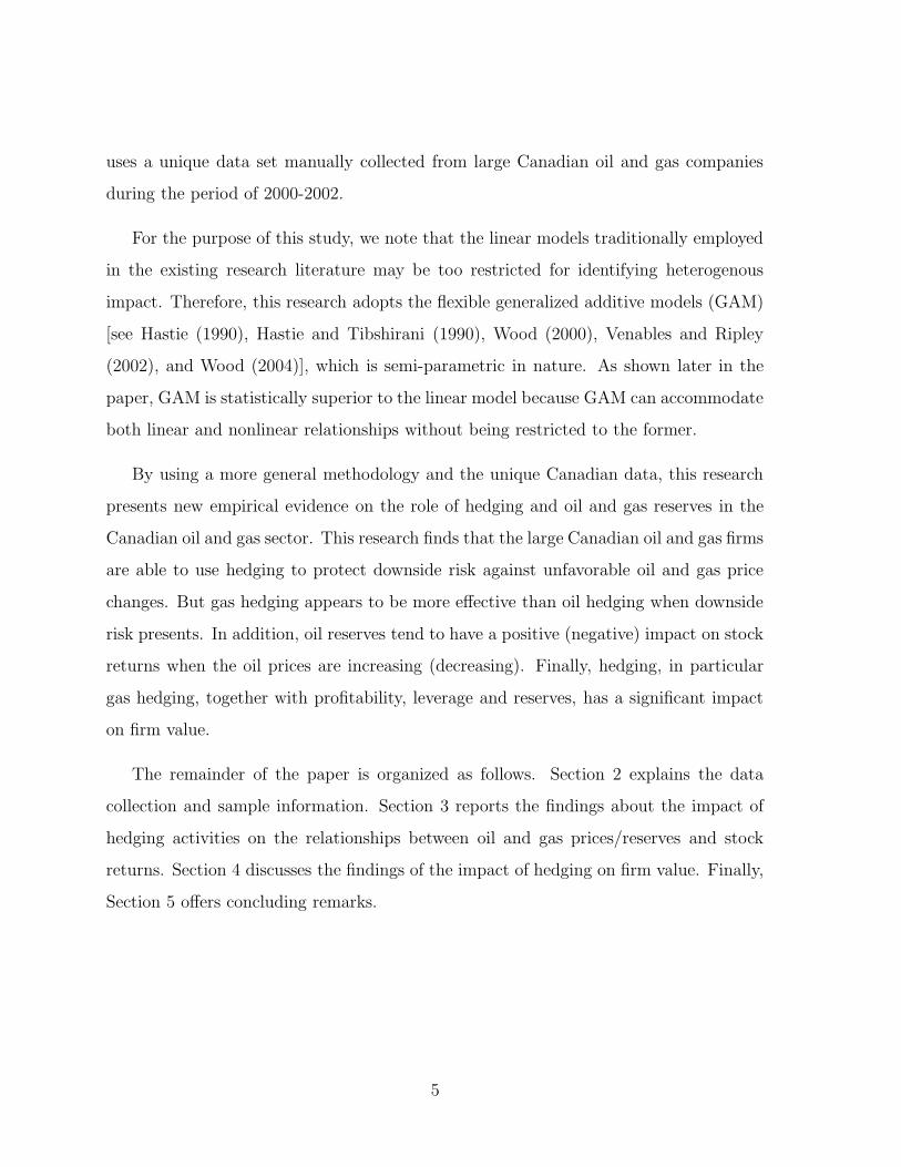
uses a unique data set manually collected from large Canadian oil and gas companies

during the period of 2000-2002.

For the purpose of this study, we note that the linear models traditionally employed

in the existing research literature may be too restricted for identifying heterogenous

impact. Therefore, this research adopts the flexible generalized additive models (GAM)

[see Hastie (1990), Hastie and Tibshirani (1990), Wood (2000), Venables and Ripley

(2002), and Wood (2004)], which is semi-parametric in nature. As shown later in the

paper, GAM is statistically superior to the linear model because GAM can accommodate

both linear and nonlinear relationships without being restricted to the former.

By using a more general methodology and the unique Canadian data, this research

presents new empirical evidence on the role of hedging and oil and gas reserves in the

Canadian oil and gas sector. This research finds that the large Canadian oil and gas firms

are able to use hedging to protect downside risk against unfavorable oil and gas price

changes. But gas hedging appears to be more effective than oil hedging when downside

risk presents. In addition, oil reserves tend to have a positive (negative) impact on stock

returns when the oil prices are increasing (decreasing). Finally, hedging, in particular

gas hedging, together with profitability, leverage and reserves, has a significant impact

on firm value.

The remainder of the paper is organized as follows. Section 2 explains the data

collection and sample information. Section 3 reports the findings about the impact of

hedging activities on the relationships between oil and gas prices/reserves and stock

returns. Section 4 discusses the findings of the impact of hedging on firm value. Finally,

Section 5 offers concluding remarks.

5

2 Data and Sample Description

There are several issues that one must face in the data selection from the universe

of the Canadian oil/gas exploration and production companies. First, the Canadian

economy has a strong resources and mining sector with many oil and gas exploration

and production firms. Many of them, however, are small exploration firms and generally

not involved in hedging activities.2 Hence we need to select relatively large and mature

oil and gas exploration and production firms which are involved in hedging activities.

Second, some of the large oil and gas companies with hedging activities are integrated

oil and gas companies. That is, they are not only involved in the oil and gas exploration

but also engaging in refinery and marketing. In order to evaluate the role of hedging

activities, it is essential to include these companies. Ignoring them would cause the loss of

valuable information and lead to a rather small sample. Third, some substantial oil and

gas players in Canada are partly owned by international corporations and partly owned

by investors in Canada (for example, Imperial Oil is partly owned by ExxonMobil in the

US, Husky Energy is partly owned by Hutchison Whampoa in Hong Kong, China, and

Shell Canada is partly owned by the Royal Dutch Shell in Holland3). These oil and gas

firms also constitute a large share of the Canadian oil and gas sector and should be duly

included. Fourth, Canadian economy is about one-tenth of the size of the US economy.

Compared with the similar studies on the US oil and gas sector, the Canadian sample

size would be considerably smaller although the oil and gas sector is a significantly large

sector in Canadian economy.

In order to find a largest relevant sample of oil and gas companies in Canada, we have

selected oil and gas companies with market value more than Cdn$500 million in 2004.4

Thirty-eight oil/gas exploration and production companies (for example, EnCana, Cana-

2Haushalter (2000) also notes that in the U.S. large oil and gas firms are more likely to hedge.3After the sample period, Shell Canada had been taken over by its parent.4The hedging activities and records of these oil and gas firms are more likely to be available and

documented systematically. SEDAR is developed in Canada for the Canadian Securities Administrators(CSA). The annual reports from SEDAR are available in www.sedar.com.

6

dian Natural Resources, Talisman Energy, and Nexen) and eight oil integrated companies

(for example, Suncor Energy, Petro-Canada, Imperial Oil, and Husky Energy) meet the

criterion. Thirty-three oil and gas companies of the above list have filed reports with

the System for Electronic Document Analysis and Retrieval (SEDAR) during the period

of 2000-2002. Thus, we have eighty-eight firm-year data, of which seventy-one firm-year

data (about 80.7%) are for oil and gas exploration and production companies and sev-

enteen firm-year data (about 19.3%) are for integrated oil companies. The largest five

companies in the sample are Encana,5 Imperial Oil, Shell Canada, Suncor Energy, and

Petro-Canada, whose average market value is Cdn$23.8 billion in 2004. The smallest five

firms are Gastar Exploration, Crescent Point Energy, Nuvista Energy, Ketch Resource,

and Pan-Ocean Energy, whose average market value is about Cdn$522 million in 2004.

Because we are interested in the hedging information of the selected firms, we use the

financial market and accounting data of these firms for the period of 2000-2002.

When we analyze the impact of hedging on the relationship between oil and gas

prices and stock returns, we use the monthly oil and gas prices from the New York

Mercantile Exchange (NYMEX) and monthly stock returns of these oil and gas firms

from Datastream. The monthly data are then combined with the annual accounting and

hedging data, which are detailed in the following part of this paper.

All the hedging information of the sample is from the annual reports of selected

companies filed at SEDAR or posted at the companies’ websites. The existing research

collect the hedging information primarily from the 10-K annual reports.6 In 1997, the

U.S. Securities and Exchange Commission (SEC) declared Financial Reporting Release

No.48 (FRR 48), which requires disclosure for market risk for all firms for the fiscal year

ending after June 15th, 1998.7 However, there is no such regulation for Canadian com-

5Encana was established from merging Alberta Energy Company Ltd. and PanCanadian EnergyCorporation in 2001.

6See, for example, Allayannis and Weston (2001) and Jin and Jorion (2006).7Under this regulation, U.S. firms are required to report in their annual reports quantitative infor-

mation on exposures of contract amounts and weighted average spot prices for forwards and futures;

7

panies at the time of the data collection. Hedging information may be found directly in

two parts of an annual report: (a) Risk Management of Management’s Discussion and

Analysis and (b) Financial Instruments in Notes of Consolidated Financial Statement

(see Appendix 1 for an example). In general, the information in Management’s Discus-

sion and Analysis highlights the hedging activities in the fiscal year. The information

in Financial Instruments in Notes of Consolidated Financial Statement details hedging

contracts such as outstanding hedging contract at the end of the fiscal year. The main

hedging instruments used by Canadian oil and gas companies are fixed-price contracts,

forwards, received-fixed swaps and options (including collars and three-way options) (see

Appendix 2 for details).

We calculate individual contract deltas and sum them up for each firm for each fiscal

year. This sum is a measure for the degree of hedging in each firm for that year. This

method of calculating each delta is detailed in Table 1. The total delta value of crude

oil and natural gas hedging for each firm-year is the sum of the products of deltas and

their corresponding notional dollar values of all hedging contracts [The notional output

measure of crude oil is expressed in barrel (bbl) and that of natural gas contracts is

presented in million of British thermal unit (mmbtu)].

The value of delta computed as such is a non-positive number. We must multiply

negative one to the value of delta to reflect the positive role of the adjusted total deltas

in the stock return and firm value. The total delta value is then scaled by the annual

production or the commodity reserves, named adjusted delta, such as the adjusted delta

of oil production and that of oil reserves. We use gas production and gas reserves as an

example to show how the adjusted deltas are defined:

Adjusted delta of gas production (Dgp) = −

(

Total delta value of gas hedging

V alue of next year gas production

)

weighted average pay and receive rates and/or prices for swaps; contract amounts and weighted averagestrike prices for options.

8

Table 1: Delta and Hedging Instruments

Delta Hedging Instrument

-1 short linear contracts, including short futures and forwards,fixed-priced contracts, fixed-received swapsand volumetric production arrangements

value from non-linear contracts, including options,Black-Scholes collars and three-way optionsoption models

Note: The value of each contract is mark to the market.

Adjusted delta of gas reserves (Dgr) = −

(

Total delta value of gas hedging

V alue of same year gas reserve

)

That is, the adjusted delta of production, Dgp, represents the percentage of next

year production that is effectively hedged, while the adjusted delta of reserves, Dgr,

gives the proportion of current reserves that is effectively hedged. We use Dop and Dor

to denote the adjusted deltas of oil production and oil reserves, respectively.

Table 2 shows the hedging and non-hedging information of the firm-years in the

sample. There are 25 non-hedging (in both oil and gas) firm-years (about 28.4% of

the sample), 56 firm-years hedging oil prices exposure (about 63.7% of the sample), 50

firm-years hedging gas prices exposure (56.8% of the sample), and 43 firm-year hedging

both oil and gas prices exposure (about 48.9% of the sample).

Table 3 illustrates the basic statistics of the adjusted deltas. In terms of the number

of the firms that hedge, Canadian oil and gas companies hedge less relative to the oil

and gas reserves than the U.S. oil and gas companies do. The average Dop, Dgp, Dor

and Dgr of the U.S. oil and gas companies are 33%, 41%, 4% and 5% respectively,

9

Table 2: Description of Firm-years: Hedging and Non-hedging

Gas: Gas: TotalHedging Non-Hedging

Firm-year Count (%) Firm-year Count (%) Firm-year Count (%)

Oil: Hedging 43 (48.9) 13 (14.8) 56 (63.7)Firm-year Count(%)

Oil: Non-Hedging 7 (8.0) 25 (28.4) 32 (36.3)Firm-year Count(%)

Total 50 (56.8) 38 (43.2) 88 (100)Firm-year Count(%)

Table 3: Basic Statistics of Adjusted Deltas

Adjust Delta Mean Standard Deviation No. of Firm-yearsOil Production (Dop) 14.6% 20.4% 88Gas Production (Dgp) 8.1% 14.8% 88

Oil Reserves (Dor) 1.8% 2.6% 88Gas Reserves (Dgr) 1.3% 2.9% 88Production Average 11.4%Reserves Average 1.6%

while those of Canadian oil and gas companies in this study are 14.6%, 8.1%, 1.8% and

1.3%, respectively.8 These numbers show that the U.S. companies are more likely to

employ risk management than their Canadian counterparts are. However, the standard

deviations of Dop and Dgp for the U.S. data are 33% and 40% respectively, higher than

those of the Canadian sample — 20.4% and 14.8%. This suggests that the large Canadian

oil and gas companies are more homogeneous in hedging than their U.S. counterparts.

8See Jin and Jorion (2006) for the U.S. numbers.

10

In this paper, we use the following equation for the Q ratio:9

Q =Book value of liabilities + Market value ofcommon equity

Book value of total assets.

The market value of common equity can be found in the Datastream database. The

book value of liabilities and total assets are from the annual reports.10

Panel A in Table 4 shows the summary statistics of total assets (in millions of Cana-

dian dollars), market value of equity (in millions of Canadian dollars), and the corre-

sponding Q ratios. The average Q ratio is 1.56, which is similar to that of the U.S.

The standard deviations of the Canadian oil and gas companies’ total assets and mar-

ket value of common equity are huge. Panels B and C of Table 4 illustrate the basic

statistics of the firms with hedging activities for oil and gas prices, respectively. On

average, these firms hedge about 23.0% of their next year oil production, which amounts

to about 3.0% of their oil reserves, and about 18.0% of their next year gas production,

which represents about 2.0% of their gas reserves. All the ratios are less than those of

the U.S. oil and gas companies. The Canadian oil and gas companies do not hedge as

much as their U.S. competitors do. The average Q ratio for oil hedging firms is 1.35,

while that of gas hedging firms is 1.31. Panel D of Table 4 shows the basic statistics of

the firms without any hedging activities. The large standard deviations of total assets

and market value of equity in non-hedging companies show that non-hedging occurs at

both large and small firms and it is not dependent on the firm size. The average Q ratio

for non-hedging firms is 2.00.

9Tobin suggested that the combined market value of all the companies on the stock market should beequal to their replacement costs [Tobin (1969) and Hayashi (1982)]. The Q ratio is theoretically definedas the market value of a firm’s assets divided by the replacement value of the firm’s assets. When theassets are priced properly in the capital market, the Q ratio should be equal to one. The change of theQ ratio is an direct measure of the change of the firm value in the capital market.

10However, several companies do not have necessary market information such as market value andstock prices during the period of 2000-2002 in the Datastream database due to mergers and corporationreconstruction. Only twenty-eight companies and seventy-six firm-years are therefore used.

11

Figure 1: Book Value of Total Asset with or without Hedging

Boo

k V

alue

(C

dn$M

illio

n)

Without Hedging With Hedging

050

0010

000

1500

020

000

2500

0

Figure 1 plots the book values of total assets of the oil and gas firms with or without

hedging. It shows that non-hedging companies vary substantially in size (both very small

and very large) while the hedging companies are concentrated in a particular range in

terms of the values of total assets. This may reflect the fact that very large firms tend

to be integrated oil companies which can diversify their operations in both up- and

down-streams of the exploration, production, and distribution processes.

12

Table 4: Basic Statistics of Adjusted Deltas

Panel A: All Firm-yearsNo. of Obs. Mean Std. Dev. Median

Total Assets (Cnd$M) 76 4019.22 5195.44 1135.98MVE (Cnd$M) 76 3574.25 4857.15 838.46

Q ratio 76 1.56 0.93 1.34Panel B: Firm-years with Hedging Activities for Oil

No. of Obs. Mean Std. Dev. MedianTotal Assets (Cnd$M) 46 4356.03 4302.58 1857.33

MVE (Cnd$M) 46 3740.24 4083.39 1406.85Dop 46 0.23 0.22 0.18Dor 46 0.03 0.03 0.02

Q ratio 46 1.35 0.49 1.26Panel C: Firm-years with Hedging Activities for Gas

No. of Obs. Mean Std. Dev. MedianTotal Assets (Cnd$M) 41 4318.25 4323.21 2001.12

MVE (Cnd$M) 41 3180.61 3350.00 1263.33Dgp 41 0.18 0.21 0.06Dgr 41 0.02 0.03 0.01

Q ratio 41 1.31 0.40 1.24Panel D: Firm-years without Hedging Activities

No. of Obs. Mean Std. Dev. MedianTotal Assets (Cnd$M) 23 3670.47 7059.76 167.30

MVE (Cnd$M) 23 3663.59 6628.01 260.50Q ratio 23 2.00 1.47 1.81

Note: Total Assets represent the book value of assets. MVE repre-sents the market value of equity. Total assets and MVE are in millionCanadian dollars (Cdn$M). Dop and Dor denote the adjusted deltasof oil production and reserves, respectively. Dgp and Dgr denote theadjusted deltas of gas production and reserves, respectively. PanelA shows the statistics for the all firm-years. The statistics for sub-samples of firm-years with hedging activities for oil and gas are re-ported, respectively, in Panels B and C. Panel D illustrates the statis-tics of firm-years without any hedging activities.

13

3 Impact of Hedging on the Relationship between

Oil and Gas Prices/Reserves and Stock Returns

In this section, we first study the relationship between oil and gas prices and stock

returns directly based on the monthly data. Then we extend the previous model in a

more general setting to examine whether or not oil and gas hedging can moderate the

impact of oil and gas price changes on stock returns.

As shown in Figure 2, monthly stock returns of hedging firms appear to have slightly

lower volatility than those of non-hedging firms during the period of 2001-2002. But it

is still unclear as what roles that hedging may play. Therefore, we need to study this in

depth using the multi-factor models.

To examine the relationship between oil and gas price changes and stock returns, we

first adopt the following model:

Rit = α + βmRmt + βoRot + βgRgt + εit (1)

where Rit is the stock return for firm i at time t; Rmt denotes the market-index return

or the S&P/TSX 60 index return at time t;11 Rot is the percentage change in the price

of NYMEX near futures contracts for oil (“oil price change” hereafter) at time t; Rgt

is the percentage change in the price of NYMEX near futures contracts for natural gas

(“gas price change” hereafter) at time t; and εit is the error term for firm i at time t in

this model. The advantage of this model is that betas associated with oil and gas price

changes may illustrate the role of hedging indirectly. If these betas are close to zero,

this indicates that stock returns are not sensitive to these price changes.

11The S&P/TSX 60 index consists of 60 largest (measured by market capitalization) and most liquid(heavily traded) stocks listed on the Toronto Stock Exchange (TSX). They are usually domestic ormultinational industry leaders in Canada.

14

Figure 2: Monthly Stock Returns with or without Hedging

0 5 10 15 20 25 30 35

−0.

60.

00.

4

Month

Rit

Stock Returns vs. Time with Hedging

0 5 10 15 20 25 30 35

−0.

60.

00.

4

Month

Rit

Stock Returns vs. Time without hedging

15

The time dummy and firm dummies are also tested in the model but they are not

statistically significant. Hence, we pool the cross-sectional and time series data to es-

timate this model. Furthermore, because of their resulting extreme Cook’s distance in

the stock return estimates, some data points (Gastar Exploration in February 2002 and

Peyto Exploration and Development in October 2001) are excluded from the sample.12

Table 5 shows the estimation results for the pooled monthly data during the period

of 2000-2002. Panel A of Table 5 reports the linear relationships that stock returns have

with oil and gas price changes. These relationships are mostly positive and statistically

significant. On average, a 1% change in oil price leads to a 0.26% change in stock returns.

This Canadian result is similar to that found by Rajgopal (1999) and Jin and Jorion

(2006). But a 1% change in gas price only leads to a 0.10% change in stock returns,

which is much lower than that of Rajgopal (1999) (0.41%) or Jin and Jorion (2006)

(0.29%). The stock returns of these Canadian companies do not respond to gas price

changes as much as they do to oil price changes. However, we note that the value of the

beta associated with the market-index return is small and statistically insignificant. At

this point, we do not know if stock returns and the market-index return could relate to

each other nonlinearly.

To explore possible nonlinear relationships, we extend our analysis by using the gen-

eralized additive model (GAM),13 which can be viewed as an extension of the generalized

linear model (GLM).14 The advantage of GAM over GLM is that GAM is a more flexible

model for identifying nonlinear effects (Please see Appendix 3 for details).

Figure 3 and Panel B of Table 5 show that the nonlinear effects of changes in oil and

gas prices on stock returns are very significant. In GAM, the χ2 test is performed to

12Cook’s distance is a metric for measuring the influential data points. A large Cook’s distance for adata point indicates that the data point is influential in the linear regression [see Chambers and Hastie(1992), p. 230].

13See Hastie (1990), Hastie and Tibshirani (1990), Wood (2000), Venables and Ripley (2002), andWood (2004).

14See McCullagh and Nelder (1989).

16

test the nonlinearity of each s function. It turns out that stock returns have nonlinear

relationships with all of the three explanatory variables. The more flexible GAM fits the

data better than the linear model and its R2-adj reaches 0.194, a substantial increase

from that of the linear model.

Figure 3 shows the estimated nonlinear effects of the explanatory variables on stock

returns. These nonlinear effects take the form of s(x, d), where s(·) represents the

marginal impact of an explanatory variable x with d degrees of smoothness (see Appendix

3 for details). For simplicity, we suppress d in s(x, d) so that we write s(x) as the marginal

impact of x on s. First, we note that s(Rmt) is quite flat when Rmt > 0. But s(Rmt)

becomes negative at Rmt = −0.10 and becomes positive at Rmt = −0.05. In other

words, stock returns of oil and gas companies do not have a linear sensitivity to the

market-index return. Clearly, this nonlinear relationship could not be identified in the

linear model. Second, we find that s(Rot) has a slightly positive slope. s(Rot) becomes

negative when Rot = −0.05 and becomes positive when Rot > 0.10. If the oil price falls

more than 5%, stock returns go down but do not fall as fast as the oil price does. If the

oil price rises more than 10%, stock returns rise but do not rise as fast as the oil price

does. This could result from some form of hedging. Third, we note that s(Rgt) has a

slight negative slope. s(Rgt) become sensitive to Rgt when Rgt < −0.20 or > 0.20. It

implies that stock returns rise when the gas price falls by 20%. However, stock returns

fall when the gas price rises more than 20%. This is an indirect evidence of some form

of hedging of gas prices.

Now we extend the previous model to examine explicitly whether or not oil and gas

hedging can moderate the impact of oil and gas price changes on stock returns:

Rit = α + βmRmt + [γ1 + γ2Dopit + γ3(ORit/MV Eit)]Rot (2)

+[γ4 + γ5Dgpit + γ6(GRit/MV Eit)]Rgt + εit

17

Table 5: Statistical Analysis of Stock Price Exposure

Panel A: Linear Three-factor Model for Stock Returns (Rit)Explanatory Variables Coefficient Std. dev. t-ratio p-value

Intercept 0.020 0.004 5.044 0.000Rmt 0.017 0.061 0.284 0.777Rot 0.263 0.050 5.318 0.000Rgt 0.095 0.025 3.810 0.000

No. of obs. 881R2-adj 0.055

Panel B: Nonlinear Three-factor Model for Stock Returns (Rit)Terms in GAM Coefficient Std. dev. t-ratio p-value

χ2 test for nonlinearityIntercept 0.024 0.003 6.967 0.000

s(Rmt, 8.51) — — 62.862 0.000s(Rot, 6.19) — — 95.146 0.000s(Rgt, 4.71) — — 20.009 0.019No. of obs. 881

R2-adj 0.194

Note: This table illustrates the estimation results of the linear coefficients andnonlinear functions in three-factor model. Panel A represents the estimationresults of the linear model:

Rit = α + βmRmt + βoRot + βgRgt + εit.

Panel B shows the estimation of the generalized additive model.

Rit = α + s(Rmt) + s(Rot) + s(Rgt) + εit.

Here Rit, Rmt, Rot, and Rgt denote the stock return of firm i at time t , themarket-index return at time t, the percentage change in the NYMEX crudeoil futures price at time t , and the percentage change in the NYMEX gasfuture price at time t, respectively. εit is the error term. The sample includesthe pooled monthly data during the period of 2000-2002. s(x, d) denotes theestimated nonlinear function of variable x with d degrees of smoothness.

18

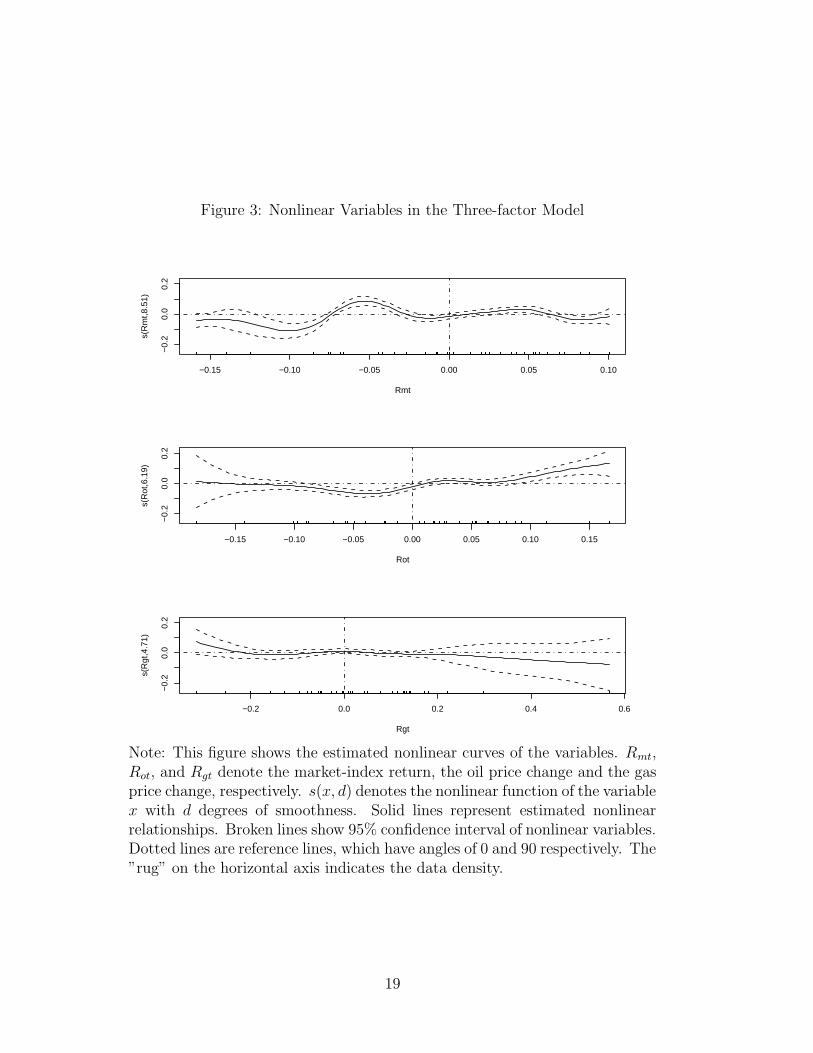
Figure 3: Nonlinear Variables in the Three-factor Model

−0.15 −0.10 −0.05 0.00 0.05 0.10

−0.

20.

00.

2

Rmt

s(R

mt,8

.51)

−0.15 −0.10 −0.05 0.00 0.05 0.10 0.15

−0.

20.

00.

2

Rot

s(R

ot,6

.19)

−0.2 0.0 0.2 0.4 0.6

−0.

20.

00.

2

Rgt

s(R

gt,4

.71)

Note: This figure shows the estimated nonlinear curves of the variables. Rmt,Rot, and Rgt denote the market-index return, the oil price change and the gasprice change, respectively. s(x, d) denotes the nonlinear function of the variablex with d degrees of smoothness. Solid lines represent estimated nonlinearrelationships. Broken lines show 95% confidence interval of nonlinear variables.Dotted lines are reference lines, which have angles of 0 and 90 respectively. The”rug” on the horizontal axis indicates the data density.

19

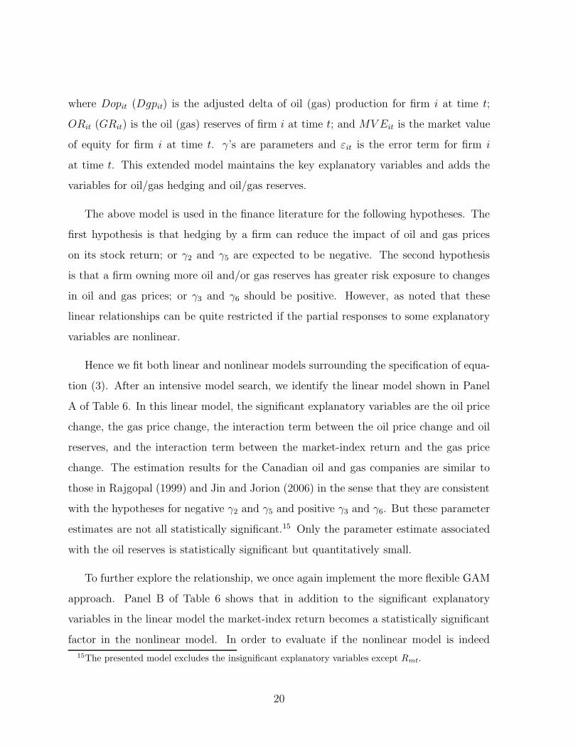
where Dopit (Dgpit) is the adjusted delta of oil (gas) production for firm i at time t;

ORit (GRit) is the oil (gas) reserves of firm i at time t; and MV Eit is the market value

of equity for firm i at time t. γ’s are parameters and εit is the error term for firm i

at time t. This extended model maintains the key explanatory variables and adds the

variables for oil/gas hedging and oil/gas reserves.

The above model is used in the finance literature for the following hypotheses. The

first hypothesis is that hedging by a firm can reduce the impact of oil and gas prices

on its stock return; or γ2 and γ5 are expected to be negative. The second hypothesis

is that a firm owning more oil and/or gas reserves has greater risk exposure to changes

in oil and gas prices; or γ3 and γ6 should be positive. However, as noted that these

linear relationships can be quite restricted if the partial responses to some explanatory

variables are nonlinear.

Hence we fit both linear and nonlinear models surrounding the specification of equa-

tion (3). After an intensive model search, we identify the linear model shown in Panel

A of Table 6. In this linear model, the significant explanatory variables are the oil price

change, the gas price change, the interaction term between the oil price change and oil

reserves, and the interaction term between the market-index return and the gas price

change. The estimation results for the Canadian oil and gas companies are similar to

those in Rajgopal (1999) and Jin and Jorion (2006) in the sense that they are consistent

with the hypotheses for negative γ2 and γ5 and positive γ3 and γ6. But these parameter

estimates are not all statistically significant.15 Only the parameter estimate associated

with the oil reserves is statistically significant but quantitatively small.

To further explore the relationship, we once again implement the more flexible GAM

approach. Panel B of Table 6 shows that in addition to the significant explanatory

variables in the linear model the market-index return becomes a statistically significant

factor in the nonlinear model. In order to evaluate if the nonlinear model is indeed

15The presented model excludes the insignificant explanatory variables except Rmt.

20

superior to its linear counterpart, the null hypothesis under which the linear model is

true is tested by the F -test based on the difference in deviances between the linear and

nonlinear models with the dispersion parameter adjustment. The resultant p-value is

close to zero. Hence the nonlinear model provides a better fit for this data. Other

model selection criteria, such as the information criterion (AIC) and the goodness of fit

(R2-adj) also confirm this choice. The chosen model has the estimated residuals close

to white noise.

In order to evaluate the nonlinear relationships implied by the two previously dis-

cussed hypotheses, we use the graphical approach for the nonlinear functions from the

semi-parametric model. Panel B of Table 6 and Figure 4 show not only what explanatory

variables are statistically significant but also how these variables affect stock returns in

nonlinear ways. The first important finding is that the hedging activities on oil and gas

in the Canadian companies appear to play little role as both DopitRot and DgpitRgt fail

to be statistically significant and hence are excluded from the chosen model.

Figure 4 shows the estimated curves and their 95% confidence intervals for statis-

tically significant nonlinear functions between the statistically significant explanatory

variables and stock returns. Specifically, Figure 4 demonstrates that the market-index

return Rmt has a nonlinear relationship with stock returns s(Rmt). This nonlinear rela-

tionship corresponds to the conventional beta for the market-index return in the linear

model. When the market-index return moves up and down by about 5%, stock returns

rise. However, when the market-index return moves, up or down, beyond the 5 % stock

returns fall.

Figure 4 shows that when the oil price Rot falls by 0-5%, stock returns s(Rot) fall.

When the oil price Rot rises by more than 10%, stock returns s(Rot) rise. There is a

positive relationship between the two but the slope of the curve is not as steep. On the

other hand, the relationship between the gas price Rgt and stock returns s(Rgt) is fairly

flat with the 95% confidence intervals covering zero although the slope of the curve is

21

slightly positive (negative) when Rgt < 0 (Rgt > 0). Both nonlinear relationships show

some non-responsiveness of stock returns to oil/gas price movements, in particular on

the downside. This is consistent with the observation obtained from the previous model

that there is an indirect evidence that some form of hedging is taking place.

Corresponding to the hypothesis that oil and gas reserves should be positively related

to stock returns in the linear model, Figure 4 shows that the relationship between oil

reserves (ORit/MV Eit)Rot and stock returns s((ORit/MV Eit)Rot) is not linear. Further,

the impact of oil reserves on stock returns is much greater in comparison with that of

other factors. Stock returns rise when oil reserves marked to the market are higher. But

when oil reserves marketed to the market are lower, stock returns fall. That is, oil and

gas reserves are more likely to have a positive (negative) impact on stock returns when

the oil and gas prices are increasing (decreasing).

Another important finding from Figure 4 is that the interaction term, RmtRgt, and

its impact on stock returns, s(Rmt.Rgt), have a convex relationship with the positive

part being statistically significant. That is, when the stock market and gas price rise or

fall at the same time, stock returns increase. In other words, stock returns can benefit

from the stock market rise and gas price hike. When the stock market and gas price

fall simultaneously, stock returns can still increase if other factors such as hedging, cost

cutting, and discovery and/or acquisition of new reserves play a significant role.

4 Hedging and Firm Value

Whether firms that hedge have a higher firm value or a higher Q ratio than those that

do not is also an important question in evaluating the role of hedging. Therefore, we

compare the values of hedging firms with those of non-hedging firms. Table 7 reports

the univariate analysis of the differences in Q ratios, book values of total asset, and

market values of equity between oil/gas hedging and non-hedging firms. Panel A and

22

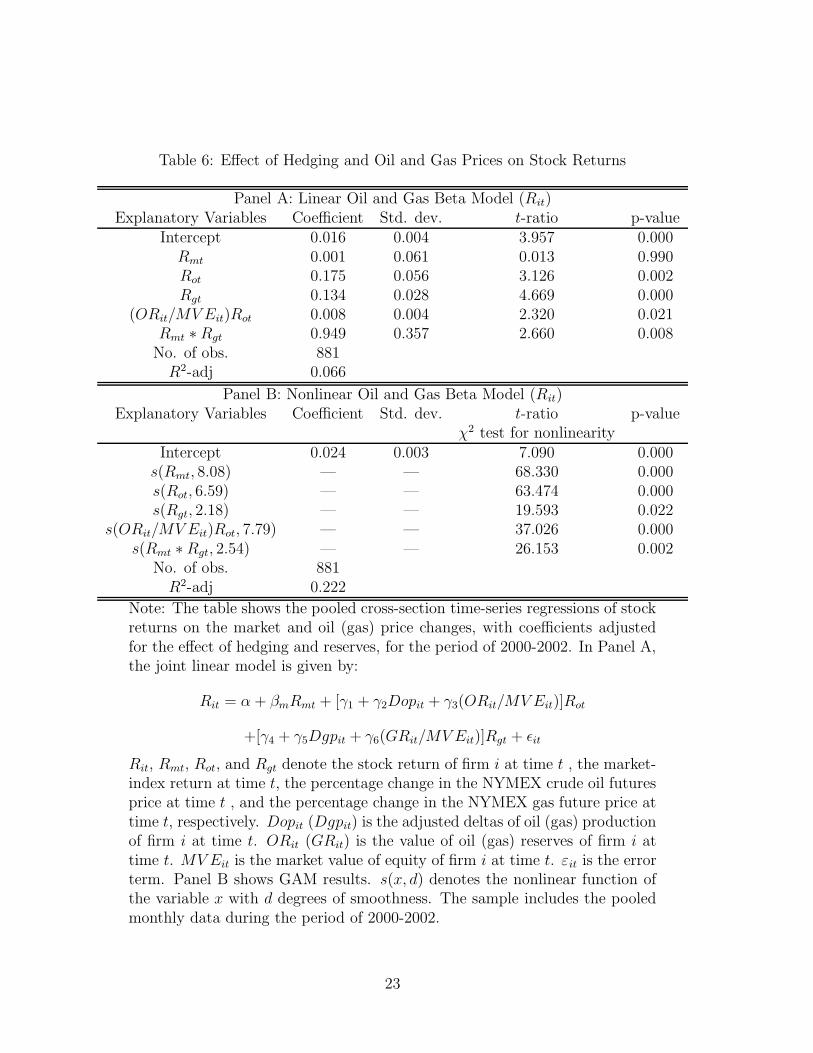
Table 6: Effect of Hedging and Oil and Gas Prices on Stock Returns

Panel A: Linear Oil and Gas Beta Model (Rit)Explanatory Variables Coefficient Std. dev. t-ratio p-value

Intercept 0.016 0.004 3.957 0.000Rmt 0.001 0.061 0.013 0.990Rot 0.175 0.056 3.126 0.002Rgt 0.134 0.028 4.669 0.000

(ORit/MV Eit)Rot 0.008 0.004 2.320 0.021Rmt ∗ Rgt 0.949 0.357 2.660 0.008

No. of obs. 881R2-adj 0.066

Panel B: Nonlinear Oil and Gas Beta Model (Rit)Explanatory Variables Coefficient Std. dev. t-ratio p-value

χ2 test for nonlinearityIntercept 0.024 0.003 7.090 0.000

s(Rmt, 8.08) — — 68.330 0.000s(Rot, 6.59) — — 63.474 0.000s(Rgt, 2.18) — — 19.593 0.022

s(ORit/MV Eit)Rot, 7.79) — — 37.026 0.000s(Rmt ∗ Rgt, 2.54) — — 26.153 0.002

No. of obs. 881R2-adj 0.222

Note: The table shows the pooled cross-section time-series regressions of stockreturns on the market and oil (gas) price changes, with coefficients adjustedfor the effect of hedging and reserves, for the period of 2000-2002. In Panel A,the joint linear model is given by:

Rit = α + βmRmt + [γ1 + γ2Dopit + γ3(ORit/MV Eit)]Rot

+[γ4 + γ5Dgpit + γ6(GRit/MV Eit)]Rgt + εit

Rit, Rmt, Rot, and Rgt denote the stock return of firm i at time t , the market-index return at time t, the percentage change in the NYMEX crude oil futuresprice at time t , and the percentage change in the NYMEX gas future price attime t, respectively. Dopit (Dgpit) is the adjusted deltas of oil (gas) productionof firm i at time t. ORit (GRit) is the value of oil (gas) reserves of firm i attime t. MV Eit is the market value of equity of firm i at time t. εit is the errorterm. Panel B shows GAM results. s(x, d) denotes the nonlinear function ofthe variable x with d degrees of smoothness. The sample includes the pooledmonthly data during the period of 2000-2002.

23

Figure 4: Nonlinear Effect of Hedging and Oil and Gas Prices on Stock Returns

−0.15 −0.05 0.05

−0.

4−

0.2

0.0

0.2

0.4

Rmt

s(R

mt,8

.08)

−0.15 0.00 0.10

−0.

4−

0.2

0.0

0.2

0.4

Rot

s(R

ot,6

.59)

−0.2 0.0 0.2 0.4 0.6

−0.

4−

0.2

0.0

0.2

0.4

Rgt

s(R

gt,2

.18)

−15 −5 0 5 10

−0.

4−

0.2

0.0

0.2

0.4

(OR/MVE)Rot

s((O

R/M

VE

)Rot

,7.7

9)

−0.02 0.00 0.02 0.04

−0.

4−

0.2

0.0

0.2

0.4

Rmt.Rgt

s(R

mt.R

gt,2

.54)

Note: This figure shows curves of the significant nonlinear relationships. Rmt(for Rmt), Rgt (for Rgt), and Rot (for Rot) denote the market-index return,the gas price change and the oil price change, respectively. (OR/MVE)Rot(for (ORit/MV Eit)Rot) denotes the sensitivities to oil reserves. Rmt.Rgt (forRmtRgt) is the interaction term between the market-index return and the gasprice change. s(x, d) denotes the nonlinear function of the variable x with ddegree freedom. Solid lines represent the estimated nonlinear relationships.Broken lines give the 95% confidence intervals of the estimated nonlinear re-lationships. Dotted lines are reference lines, which have angles of 0 and 90respectively. The ”rug” on the horizontal axis indicates the data density.

24

B of Table 7 show the basic statistics for the oil hedging firms with respect to non-oil

hedging and non-hedging firms, respectively. The similar analysis is reported for the

gas hedging firms with respect to non-gas hedging and non-hedging firms, respectively

in Panel C and D. Table 7 shows that the differences between hedging and non-hedging

firms are primarily in the Q ratio and that the firms with oil and gas hedging tend to

have lower Q ratios.

However, the Q ratio is likely to be determined by many different factors and hence

we adopt the following more general framework:

lnQit = α + β1(Oil Heding Dummy)it + β2(Gas Hedging dummy)it (3)

+β3Dopit + β4Dorit + β5Dgpit + β6Dgrit + γ(Control V ariables)it + εit,

where subscript i is for firm i and subscript t is for time t.

As in Allayannias and Weston (2001) and Jin and Jorion (2006), the control vari-

ables are return on asset, investment growth, access to financial markets, leverage, and

production cost. Return on assets (Roa) is measured by the ratio of net income to book

value of total assets. It is expected to have a positive association with the Q ratio be-

cause highly profitable firms tend to have a high Q ratio. Investment growth is measured

by the ratio of capital expenditure to book value of total assets. It is expected to have

a positive coefficient because firm value depends more on future investment. Access to

financial market is measured by a dividend dummy variable that equals 1 if the firm has

paid a dividend in the current year, 0 otherwise. There are two different views on the

information role of dividend payment. Some suggest that dividend-paying firms are less

financially constrained and may invest in less optimal projects. Hence, they have lower

Q ratios [see Allayannis and Weston (2001)]. Others argue that dividend-paying firms

typically have good management and hence higher Q ratios [see Jin and Jorion (2006)].

Leverage is measured by the ratio of book value of long-term debt to market value of

25

Table 7: Comparison of Firm Values between Hedging and Non-hedging Firms

Panel A: Oil Hedging and Non-oil Hedging FirmsVariables Hedging Non-hedging Difference t-test (mean) p-value

(46 obs.) (30 obs.) Z-test (median)Q(mean) 1.35 1.87 -0.52 -2.09 0.04

Q(median) 1.27 1.55 -0.28 -2.27 0.02BV(mean) 4356.03 3502.78 853.25 0.64 0.52

BV(median) 1857.33 433.20 1424.13 2.66 0.01MVE(mean) 3740.24 3319.73 420.51 0.34 0.74

MVE(median) 1406.85 488.68 918.17 2.01 0.04

Panel B: Oil Hedging and Non-hedging FirmsVariables Hedging Non-hedging Difference t-test (mean) p-value

(46 obs.) (23 obs.) Z-test (median)Q(mean) 1.35 2.00 -0.65 -2.05 0.05

Q(median) 1.27 1.81 -0.55 -1.97 0.05BV(mean) 4356.03 3670.47 685.56 0.43 0.67

BV(median) 1857.33 167.30 1690.03 2.83 0.00MVE(mean) 3740.24 3663.59 76.65 0.05 0.96

MVE(median) 1406.85 260.50 1146.35 2.09 0.04

Panel C: Gas Hedging and Non-gas Hedging FirmsVariables Hedging Non-hedging Difference t-test (mean) p-value

(41 obs.) (35 obs.) Z-test (median)Q(mean) 1.31 1.85 -0.54 -2.47 0.02

Q(median) 1.24 1.75 -0.51 -2.63 0.01BV(mean) 4318.25 3668.93 649.33 0.53 0.60

BV(median) 2001.12 540.60 1460.52 2.82 0.00MVE(mean) 3180.61 4035.37 -854.76 -0.73 0.47

MVE(median) 1263.33 439.05 824.28 1.74 0.08

Panel D: Gas Hedging and Non-hedging FirmsVariables Hedging Non-hedging Difference t-test (mean) p-value

(41 obs.) (23 obs.) Z-test (median)Q(mean) 1.31 2.00 -0.69 -2.21 0.04

Q(median) 1.24 1.81 -0.57 -2.14 0.03BV(mean) 4318.25 3670.47 647.79 0.40 0.69

BV(median) 2001.12 167.30 1833.82 3.04 0.00MVE(mean) 3180.61 3663.59 -482.98 -0.33 0.75

MVE(median) 1263.33 260.50 1002.83 2.38 0.02Note: This compares means and medians of Q ratios (Q), book values (BV) of total asset and market values of equity(MVE) between hedging and non-hedging companies. Panels A and B show the comparison between oil hedging companiesand non-oil hedging and non-hedging companies respectively. Similarly, Panels C and D show the comparisons between gashedging companies and non-gas hedging and non-hedging companies respectively. A t-test assuming unequal variances isused for comparing means. Wilcoxon ranksum Z-test is used for comparing medians. Two-side p-values are reported. BothBV and MVE are in million Canadian dollar (Cdn$M).

26

common equity. It is expected to be negatively related to the Q ratio. Production cost

refers the cost of extracting oil and gas as reported in annual reports. This variable is

expected to be negatively related with the Q ratio [see Jin and Jorion (2006)]. Although

the book value of total asset can be a reasonable proxy for firm size, we do exclude this

variable as a control variable in the model to avoid the endogenous problem because the

Q ratio is also directly linked to the book value.

Table 8 illustrates the regression results for both linear and nonlinear models after

an intensive model search. The resulting linear model is nested in the selected nonlinear

model. Based on the AIC, R2 and R2-adj, the nonlinear model has a better fit for

the data. The tests based on the difference in deviance and the F-tests also support

the conclusion that the nonlinear model, which is the mixture of linear and nonlinear

relationships, is superior to the linear model.

Table 8 shows that both selected linear and nonlinear models do not include the fol-

lowing explanatory variables: investment growth, assess to financial market, production

cost, delta values relative to oil production and reserves, and oil and gas hedging dummy

variables. These variables, if included in the model, are not statistically significant.

Table 8 shows that in both selected linear and nonlinear models only return on assets,

leverage, adjusted delta of gas production, and adjusted delta of gas reserves are statisti-

cally significant. R2-adj of the nonlinear model is 0.359, higher than that of the linear

model (0.242). The nonlinear model contains both linear and nonlinear relationships.

Firm value has a positive linear relationship with return on asset and adjusted delta of

gas reserves, a negative linear relationship with adjusted delta of gas production, and a

nonlinear relationship with leverage.

Because our chosen GAM is fitted on the logarithm of the Q ratio, these partial

effects of these explanatory variables may be interpreted as multiplicative explanatory

variables for the Q ratio itself. Each penal in Figure 6 shows the partial effect of the

explanatory variable on ln Q while holding other explanatory variables fixed. When Roa

27

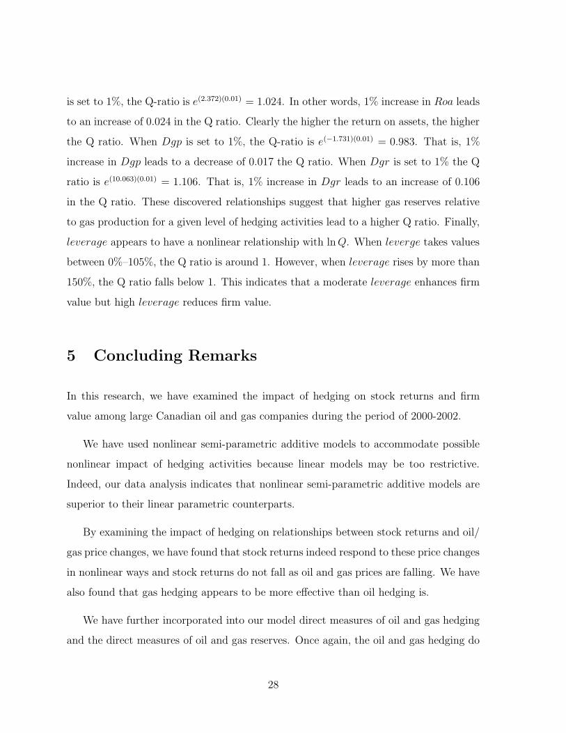
is set to 1%, the Q-ratio is e(2.372)(0.01) = 1.024. In other words, 1% increase in Roa leads

to an increase of 0.024 in the Q ratio. Clearly the higher the return on assets, the higher

the Q ratio. When Dgp is set to 1%, the Q-ratio is e(−1.731)(0.01) = 0.983. That is, 1%

increase in Dgp leads to a decrease of 0.017 the Q ratio. When Dgr is set to 1% the Q

ratio is e(10.063)(0.01) = 1.106. That is, 1% increase in Dgr leads to an increase of 0.106

in the Q ratio. These discovered relationships suggest that higher gas reserves relative

to gas production for a given level of hedging activities lead to a higher Q ratio. Finally,

leverage appears to have a nonlinear relationship with ln Q. When leverge takes values

between 0%–105%, the Q ratio is around 1. However, when leverage rises by more than

150%, the Q ratio falls below 1. This indicates that a moderate leverage enhances firm

value but high leverage reduces firm value.

5 Concluding Remarks

In this research, we have examined the impact of hedging on stock returns and firm

value among large Canadian oil and gas companies during the period of 2000-2002.

We have used nonlinear semi-parametric additive models to accommodate possible

nonlinear impact of hedging activities because linear models may be too restrictive.

Indeed, our data analysis indicates that nonlinear semi-parametric additive models are

superior to their linear parametric counterparts.

By examining the impact of hedging on relationships between stock returns and oil/

gas price changes, we have found that stock returns indeed respond to these price changes

in nonlinear ways and stock returns do not fall as oil and gas prices are falling. We have

also found that gas hedging appears to be more effective than oil hedging is.

We have further incorporated into our model direct measures of oil and gas hedging

and the direct measures of oil and gas reserves. Once again, the oil and gas hedging do

28

Table 8: Hedging and Firm Value

Linear Model

Explanatory Coefficient Std. dev. t-ratio p-valueVariable

Intercept 0.437 0.085 5.173 0.000Dgp -1.857 0.704 -2.640 0.001Dgr 10.003 3.735 2.679 0.009Roa 1.845 0.578 3.194 0.002

Leverage -0.685 0.182 -3.763 0.000No. of Obs. 76

R2-adj 0.242

Nonlinear Model

Explanatory Coefficient Std. dev. t-ratio p-valueVariable χ2 test

for nonlinearity

Intercept 0.194 0.063 3.070 0.003Dgp -1.731 0.660 -2.623 0.011Dgr 10.063 3.492 2.882 0.005Roa 2.372 0.563 4.213 0.000

s(Leverage, 6.363) — — 37.671 0.000No. of Obs. 76

R2-adj 0.359

Note: This table shows the selected linear and nonlinear regression mod-els for analyzing the impact of hedging on firm value. These models arevariants of the following specification:

lnQit = α + β1(Oil Heding Dummy)it + β2(Gas Hedging dummy)it

+β3Dopit +β4Dorit +β5Dgpit +β6Dgrit +γ(Control V ariables)it + εit,

This sample includes twenty-eight firms and seventy-six firm-years from2000 to 2002. Dgp is the delta value relative to gas production. Dgr isthe delta value relative to gas reserves. Roa is the ratio of net incomeover book value of total asset. Leverage is measured by the book valueof long-term debt to market value of common equity. s(Leverage, 6.363)denotes the nonlinear function of the variable leverage with 6.363 degreesof smoothness.

29

Figure 5: Linear and Nonlinear Relationships for Firm Value

−0.2 −0.1 0.0 0.1 0.2

−1

01

2

Roa

s(R

oa,1

)

0.0 0.5 1.0 1.5

−1

01

2leverage

s(le

vera

ge,6

.36)

0.0 0.1 0.2 0.3 0.4 0.5

−1

01

2

Dgp

s(D

gp,1

)

0.00 0.05 0.10 0.15

−1

01

2

Dgr

s(D

gr,1

)

Note: This figure shows the estimated linear and nonlinear relationships insolid lines for ln Q. Roa is the ratio of net income to book value of total asset.The partial impact of Roa on lnQ [s(Roa, 1)] is linear. Leverage is measuredby the ratio of book value of long-term debt to market value and has a nonlinearrelationship with ln Q [s(Leverage, 3.36)]. The higher the leverage is, the lowerthe firm value is. Dgp denotes the delta value relative to gas production and ithas a negative linear relationship with ln Q [s(Dgp, 1)]. Dgr denotes the deltavalue relative to gas reserves and it has a positive linear relationship with ln Q[s(Dgr, 1)]. Broken lines give the 95% confidence intervals of the estimatednonlinear relationships. Dotted lines are reference lines, which have angles of0 and 90 respectively. The ”rug” on the horizontal axis indicates the datadensity.

30

not have strong influence on stock returns as the oil and gas reserves do. The evidence

shows that Canadian oil and gas firms are able to hedge against some down side risk such

as unfavorable changes in oil and gas prices. In addition, oil reserves are more likely

to have a positive (negative) impact on stock returns when oil prices are increasing

(decreasing).

Finally, we have examined the impact of hedging on firm value measured by Tobin’s

Q ratio using both linear and nonlinear models. We have found that profitability (return

on assets) has a positive impact on firm value and that excess leveraging has a negative

impact on firm value. In addition, for a given level of gas hedging, higher gas reserves

relative to gas production lead to a higher Q ratio.

There are several other issues left for future studies. First, the hedging information

from annual reports may be incomplete as some companies may under-report their hedg-

ing activities in their annual reports. Second, most of Canadian oil and gas companies

export oil and gas directly to the U.S. and many of them may rely on hedging on foreign-

exchange-rate exposure rather than oil-and-gas-price exposure. These interesting issues

are left for future research.

31

References

[1] Adam, T.R. (2002), “Do firms use derivatives to reduce their dependence on external

capital markets?” European Finance Review 6, 163-187.

[2] Allayannis, George and A. Mozumdar (2000), “Cash flow, investment, and hedg-

ing.” Working Paper, Darden School of Business, University of Virginia.

[3] Allayannis, George and James P. Weston (2001), “The use of foreign currency

derivatives and firm market value.” Review of Financial Studies 14, 243-276.

[4] Bartram, Sohnke, Gregory Brown and Frank Fehle (2006), “International evidence

on financial derivatives usage.” forthcoming in Financial Management.

[5] Carter, David A., Daniel A. Rogers, and Betty J. Simkins (2006), “Does fuel hedging

affect firm value? Evidence from the U.S. airline industry.” Financial Management

35, 53–86.

[6] John M. Chambers and Trevor J. Hastie (1992), Statistical Models in S, Pacific

Grove, California: Wadsworth & Brooks.

[7] DeMarzo, P., and D. Duffie (1995), “Corporate incentives for hedging accounting.”

Review of Financial Studies 95, 743-771.

[8] Dionne, Georges, and Thouraya Triki (2005), “Risk management and corporate

governance: The importance of independence and financial knowledge for the board

and the audit committee.” HEC Montreal, Canada.

[9] Froot, Kenneth A., David S. Scharfstein, and Jeremy C. Stein (1993), “Risk man-

agement: coordinating corporate investment and financing policies.” Journal of

Finance 48, 1629-1658.

[10] Gagnon, Louis, Gregory J. Lypny, and Thomas H. McCurdy (1998), “Hedging

foreign currency portfolio,” Journal of Empirical Finance 5, 197-220.

32

[11] Geczy, Christopher, Bernadette A. Minton, and Catherine Schrand (1997), “Why

firms use currency derivatives?” Journal of Finance 52, 1323-1354.

[12] Graham, John R. and Daniel A. Rogers (2002), “Do firms hedge in response to tax

incentives?” Journal of Finance 57, 815-839.

[13] Graham, John R. and C.W. Smith (1999), “Tax incentives to hedge.” Journal of

Finance 54, 2241-2262.

[14] Hastie, T. J. (1990), “Generalized additive models.” Chapter 7 in J. M. Chambers

and T. J. Hastie (eds.) Statistical Models in S, Pacific Grove, California: Wadsworth

& Brooks.

[15] Hastie, T. and R. Tibshirani. (1990), Generalized Additive Models, London: Chap-

man and Hall.

[16] Haushalter, G. David (2000), “Financing policy, basis risk, and corporate hedging:

Evidence from oil and gas producers.” Journal of Finance 55, 107-152.

[17] Hayashi, Fumio (1982), “Tobin’s marginal q and average q: A neoclassical interpre-

tation.” Econometrica 50, 213-224.

[18] Jin, Y., and P. Jorion (2006), “Firm value and hedging: Evidence from U.S oil and

gas producers.” Journal of Finance 61, 893-919.

[19] Jorion, Philippe (1990), “The exchange-rate exposure of U.S. multinationals.” Jour-

nal of Business 63, 331-345.

[20] Mayers, David, and Clifford Smith (1990), “On the corporate demand for insurance:

Evidence from the reinsurance market.” Journal of Business 63, 19-40.

[21] McCullagh, P. and J. A. Nelder(1989), Generalized Linear Models. Second Edition,

London: Chapman and Hall.

33

[22] Rajgopal, Shivaram (1999), “Early evidence on the informativeness of the SEC’s

market risk disclosures: The case of commodity price risk exposure of oil and gas

producers.” Accounting Review 74, 251-280.

[23] Smith, Clifford W. and Rene M. Stulz (1985), “The determinants of firm’s hedging

policies.” Journal of Financial and Quantitative Analysis 20, 391-405.

[24] Stulz, Rene M. (1984), “Optimal hedging policies.” Journal of Financial and Quan-

titative Analysis 19, 127-140.

[25] Stulz, Rene M. (1990), “Managerial discretion and optimal hedging policies.” Jour-

nal of Financial Economics 26, 3-27.

[26] Tobin, James (1969), “A general equilibrium approach to monetary policy.” Journal

of Money, Credit and Banking 1, 15-29.

[27] Tufano, Peter (1996), “Who manages risk? An empirical examination of risk man-

agement practices in the gold mining industry.” Journal of Finance 51, 1097-1137.

[28] Venables, W. N. and B. D. Ripley (2002), Modern Applied Statistics with S, (New

York: Springer).

[29] Whidbee, David and Mark Wohar (1999), “Derivative activities and managerial

incentives in the banking industry.” Journal of Corporate Finance 5, 251-276.

[30] Wood, Simon N. (2000), “Modelling and smoothing parameter estimation with

multiple quadratic penalty.” Journal of Royal Statistical Scoiety B 62 Part 2, 413-

428.

[31] Wood, Simon N. (2004), “Stable and efficient multiple smoothing parameter esti-

mation for generalized additive models.” Journal of the American Statisitcal Asso-

ciation 99, 673-686.

34

Appendix 1 Hedging Information in 2002 Annual Report of Acclaim En-

ergy Trust

A. Information in Management’s Discussion & Analysis

COMMODITY MARKETING AND PRICE RISK MANAGEMENT

Upon closing the acquisition of Elk Point, Acclaim’s natural gas weighting increased

to 53 percent of production, while conventional oil and NGLs and heavy oil comprise 39

percent and 8 percent respectively.

· · · · · ·

WTI averaged US$26.11 per bbl in 2002, a slight increase to the average of US$25.97

per bbl in 2001. Acclaim’s price is also influenced by the Canadian$/US$ exchange rate

as well as the degree of gravity of the oil and hedging activity. The majority of Acclaim’s

production is classified as light oil which trades at a premium relative to medium and

heavy oil. Early in 2003, the benchmark WTI has been very strong averaging US$34.86

per bbl in the first quarter due primarily to uncertainties associated with the conflict in

the Middle East.

· · · · · ·

As of March 2003, Acclaim had hedging contracts in place originating from Acclaim,

Ketch Energy, Elk Point and various predecessor companies. Since the combination of

Acclaim with Ketch Energy, the Trust has layered on additional marketing contracts

and will continue to do so on an ongoing basis, in order to maintain the stability of

long-term cash distributions.

B. Information in Notes of Consolidated Financial Statement

15. HEDGING AND FINANCIAL INSTRUMENTS

35

The Trust’s financial instruments recognized on the consolidated balance sheets in-

clude accounts receivable, accounts payable and accrued liabilities, bank debt and hedg-

ing and capital lease obligations. The fair values of financial instruments other than

bank debt approximates their carrying amounts due to the short-term nature of these

instruments. The carrying value of bank debt approximates its fair value due to floating

interest terms; the fair value of the obligation under capital lease approximates carrying

value due to current rates for comparable terms of the lease obligation. The fair value

of the interest rate swaps associated with bank debt is disclosed in Note 6.

The Trust is exposed to the commodity price fluctuations of crude oil and natural

gas and to fluctuations of the Canada - US dollar exchange rate. The Trust manages this

risk by entering into various on and off balance sheet derivative financial instruments. A

portion of the Trust’s exposure to these fluctuations is hedged through the use of swaps

and forward contracts. The Trust’s exposure to interest rate fluctuations is disclosed

in Note 6. The Trust is exposed to credit risk due to the potential non-performance of

counter parties to the above financial instruments. The Trust mitigates this risk by deal-

ing only with larger, well-established commodity marketing companies and with major

national chartered banks. As a result of commodity hedging transactions, petroleum

and natural gas sales for 2002 increased by $0.5 million (2001 - $5.5 million).

December 31, 2002 outstanding contracts (see the following table)

36

Crude Oil: Outstanding Contracts

Financial Instrument Daily Volume Floor/Ceiling Term

(bbls)

Three way collar 1,000 US$20.00–25.00–29.00 Jan.1, 2003–Jul.31, 2003

Three way collar 1,000 US$22.00–24.00–28.60 Jan.1, 2003–Dec.31, 2003

Collar 500 US$22.00–29.00 Jan.1, 2003–Dec.31, 2003

Collar 500 US$22.00–29.50 Jan.1, 2003–Dec.31, 2003

Collar 500 US$24.00–29.00 Jan.1, 2003–Jun.30, 2003

Collar 500 US$24.00–29.07 Jan.1, 2003–Jun.30, 2003

37

Appendix 2 Hedging Instruments

In hedging activities, fixed-price contracts, forwards, received-fixed swaps and options

(including collars and three-way options) are the main instruments used by Canadian

oil and gas companies.

A fixed-price contract obliges the supplier to deliver a defined commodity to a con-

sumer at a predetermined price. Many such contracts include significant penalties for

non-delivery. A fixed-price contract shifts most or all risks from the buyer to the supplier,

and simultaneously shifts the management burden from the buyer to the supplier.

Forward or a forward contract is an over-the-counter contractual obligation to buy

or sell a financial instrument/a commodity at an agreed price and to make a payment

or a delivery at a pre-set future time between the two counterparties. Forward contracts

generally are arranged to have zero mark-to-market value at inception, although they

may be off-market. Examples include forward foreign exchange contracts in which one

party is obligated to buy foreign exchange from another party at a fixed rate for delivery

on a pre-set date. Off-market forward contracts are often used in structured combina-

tions, with the value on a forward contract offsetting the value of another instrument or

other instruments.

Received-fixed commodity swaps are the swaps in which exchanged flows are depen-

dent on the prices of a commodity (or an underlying commodity index). The commodity

producer who wishes to avoid the commodity price fluctuation can engage in this kind

of swaps by paying a fee to a financial institution that is willing to pay the producer the

fixed payments for the commodity and accept the commodity price fluctuation.

A collar, or a zero cost collar option, is a positive-carry collar that secures a return

through the purchase of a floor and sale of a cap. An example of a zero cost option collar

for selling commodity is the purchase of a put option and the sale of a call option with a

higher strike price. The sale of the call will cap the return if the price of the underlying

38

commodity rises, but the premium collected from the sale of the call will offset the cost

of the purchased put.

The three-way options is an option strategy created by adding to a collar, another

long put (call) option position whose strike price is lower (higher) than that of put (call)

option in the collar to benefit from falling (rising) prices. In other words, the motive of

those hedging activities for each oil and gas companies is to sell oil and gas with ideal

prices.

39

Appendix 3 General Additive Models

Let the sample counterparts of random variables

Y, X1, X2, . . . , Xp

be

y, x1, x2, . . . , xp.

The GAM takes the following functional form:

g[µ(x1, x2, . . . , xp)] = α + s1(x1) + · · · + sp(xp), (4)

where µ(x1, x2, . . . , xp) = E(Y |X1, X2, . . . , Xp), g is the link function, α is a constant,

and s is a continuous and twice differentiable function. When Y is a real valued variable

and the error is assumed to be Gaussian, and the link function g is the identity function,

the GAM is reduced to the additive model as follows

E(Y |X1, · · · , Xp) = α + s1(x1) + · · ·+ sp(xp). (5)

The above structure regression can be deemed as the first order analysis of variance

(ANOVA) decomposition of E(Y |X1, · · · , Xp) = s(x1, . . . , xp) in a p-dimensional real

space Rp.

The nonlinear functions sj(xj)(j = 1, . . . , p) are estimated jointly by the backfitting

algorithm. This algorithm minimizes a penalized residual sum of squares

PRSS(α, s1,···,sp) =N∑

i=1

yi − α −p∑

j=1

sj(xj)

2

+p∑

j=1

λj

∫

s′′

j (tj)2dtj (6)

40

by iteratively fitting nonlinear functions sj(xj)(j = 1, · · · , p) using a one dimensional

natural spline with its smoothness controlled by the penalty term

λj

∫

s′′

j (tj)2dtj.

The tuning parameter λj can be either pre-specified or automatically searched in each

step by minimizing the generalized cross-validation (GCV) score. Sometimes we write

sj(xj) as s(xj, dj) where dj is the degree of smoothness. dj may be non-integer. A more

recent version of GAM fitting implemented in the mgcv package in R by Wood (2000,

2004) selects the multiple smoothing parameters more efficiently through minimization

of the GCV score. This package employs a Bayesian approach to estimate the variance

so that it makes the confidence interval calculation for s(xj, dj)(j = 1, . . . , p) easier.16

16See Wood (2000) for details.

41