the impact of loss incidence on analyst forecast

The Impact of Loss Incidence on Analyst Forecast Dispersion: Uncertainty or Information Asymmetry

Jorida Papakroni

Franklin and Marshall College

In this study we examine the effect of loss incidence on the analyst earning’ forecast dispersion, using annual data for US firms over the period 1986-2011. We find strong positive relationship between the loss incidence and forecast dispersion even when controlling for financial distress. We argue that the significant impact of losses on the analysts’ earnings forecast dispersion is due to a combination of both higher information asymmetry and higher uncertainty regarding the future value of the firm. As such, our study provides a possible reconciliation for the different results provided by Ertimur (2004) and Ciccone (2001) about the incidence of losses. INTRODUCTION

In their seminal work, Miller and Modigliani (1966) discuss how the investors make use of the accounting earnings to infer the power of the firms’ assets to generate future cash flows. Moreover, they argue that losses reduce this predicting ability of the accounting earnings and complicate the earnings-based evaluation models. Concerned with the increase in the trend of losses1, more studies focus on the causes and consequences of losses. For example, Hayn (1995) shows that the market reaction to a loss is systematically different compared to positive earnings. Even though prior literature2 examines the impact of losses on earnings and returns, very little work has been done in the literature on how the loss incidence affects the information structure of the firm and the implications on the market efficiency. The objective of this paper is to investigate whether relative to the profit firms, those firms that report losses (either single or multiple) experience a higher level of information asymmetry among investors. The main proxy for the asymmetric information is the analysts’ earnings forecast dispersion, which refers to the disagreement among analysts with regard to the expected earnings per share (EPS) of a given firm.

In order to study this relationship, we follow Ertimur’s (2004) approach in categorizing the sample firms into three groups depending on their loss status: profit firms, single loss firms and multiple loss firms. She documents that single loss firms have, on average, higher bid-ask spreads than profit firms and multiple loss firms have higher bid-ask spreads than single loss firms. But, differently from her, we use the standard deviation of analyst earnings’ forecasts (hereafter the forecast dispersion) to proxy for the information asymmetry. In addition, taking into consideration the critique from Ciccone (2001), who argues that forecast dispersion is positively related to financial distress and business risk, we also control for poor financial performance and uncertainty before capturing the effect of information quality surrounding the loss firms.

For our empirical tests we focus on the loss observations from 1986 to 2011 for U.S. firms excluding financial and utilities companies. The choice of sample period reflects the availability of all data sources.

26 Journal of Accounting and Finance vol. 13(5) 2013

We use several econometric frameworks to test our hypothesis like Least Square, Fama-MacBeth and Panel Regressions with firm and time fixed effects. In addition we provide analysis for different testing windows and different definitions of the dependent variable. Consistent with our hypothesis we show that the positive relationship between the loss incidence and forecast dispersion is driven by losses and not financial distress, for both the level and the decomposed measures of forecast dispersion. However, we do not find any significant relationship between reported losses and the change of analysts’ earnings forecast dispersion.

This study establishes the following contributions in the literature. First, we add to the literature on the determinants of analysts’ forecasts properties by documenting a positive significant relationship between loss incidence and analysts’ earnings forecast dispersion. Second, we extend the findings of Ertimur’s (2004) by providing new empirical evidence that losses translate into higher levels of information asymmetry among the investors, when proxied by analysts’ earnings forecast dispersion, due to a decline in the accounting information. Finally, we provide a unique decomposition of the measure of analysts’ earnings forecast dispersion into uncertainty and asymmetric information using bid-ask spreads. Our results show that the significant positive impact of losses on analysts’ earnings forecast dispersion is due to a combination of both higher information asymmetry and higher uncertainty regarding the future value of the firm, providing a possible reconciliation between the findings of Ciccone (2001) and Ertimur (2004).

The remainder of this paper is organized as follows. Section 2 provides a discussion on prior research on losses and asymmetric information and motivates the hypothesis. Section 3 explains the research design. We report the empirical results in Sections 4. Finally, Section 5 draws conclusions from our study. PRIOR LITERATURE AND HYPOTHESIS DEVELOPMENT

Ramnath et al. (2008) and Clarke and Shastri (2001) provide a general review of empirical research that makes use of different properties of the analyst earnings’ forecasts such as the forecast error3, consensus4 and dispersion as proxies for the information quality surrounding a firm. In our paper we focus on the analyst earnings’ forecast dispersion, which refers to the disagreement among analysts with regard to the expected earnings per share (EPS) of a given firm. Since forecast dispersion reflects the analysts’ expectations about the firm’s future profitability, it is a forward looking variable and as such can be easily distinguished from other asymmetric information proxies like bid-ask spread and PIN. Prior research5 argues that a lack of public available information about a firm results in a higher disagreement among analysts that is reflected as a higher dispersion of analysts’ forecasts. However, even when the information is publicly available, analysts will use their individual (private) knowledge to issue forecasts that contain new-analyst specific information or interpretation. In support of this argument, Barron et al. (2002) find evidence that the degree of consensus among analysts’ forecasts is lower for high-intangible firms.

Although not immune to criticism6, our choice of analysts’ earnings forecast dispersion as a proxy for information asymmetry is based on two main assumptions. First, we assume that the degree to which analysts possess private information also reflects the degree of information asymmetry between informed and uninformed investors. In their forecasting process, analysts use various sources of information about the firms, including periodic financial statements, SEC filings, industrial reports, macro-economic news, conference calls and management communications (Ramnath et al., 2008). However, analysts with access to private information or with the analytical ability to extract private information from the publicly available are able to produce forecasts that contain new analyst-specific information or interpretation7.

Our second assumption is that if a firm discloses high quality information, this is easily processed and analyzed by the analysts. In this case, all the analysts will infer very similar predictions about the firm’s future earnings, which translate into low analysts’ earnings forecast dispersion. However, if the firm holds back information or discloses information subject to interpretation, this gives analysts an incentive to acquire private information or develop more sophisticated models about their predictions. As such we

Journal of Accounting and Finance vol. 13(5) 2013 27

expect a higher disagreement among analysts about the firms’ EPS forecasts, resulting in a higher measure of forecast dispersion.

In this paper we argue that loss firms are surrounded by higher levels of asymmetric information. Previous research provides two possible explanations for the positive association between loss incidence and asymmetric information: (1) the decline in the accounting information content of the firm and/or (2) the negative impact of the information disclosure.

First, when firms report losses, it complicates the earnings-based evaluation models and reduces the predicting power of accounting information (Miller & Modigliani, 1966). Moreover, Hayn (1995) empirically shows that the explanatory power of earnings for returns significantly declines when loss firms are taken into consideration. She finds that lower information content of losses can be explained by the stock liquidation option that the shareholders have if the loss continues in the future. She argues that faced with a reported loss the investors may assign more weight to alternative accounting information in the process of equity valuation. This suggests that although a net operating loss is public information it becomes less precise, resulting in higher levels of information asymmetry surrounding the firm that reports the loss, captured by higher forecast dispersion.

Second, managers of the firms that report losses may try to hide information using certain types of earnings management that add noise to earnings. These management practices affect negatively the information disclosure and positively the asymmetric information. Theoretical models by Verrecchia (1983), Dye (1986) and Shin (2003), and empirical research by Anilowski et al. (2007) and Kothari et al. (2009), suggest that under certain conditions firms have incentives to engage in selective disclosure by releasing good news about future earnings while delaying bad news.

Finally, a few more studies provide some evidence that loss firms try to supplement the decline in information content by voluntarily disclosing more information in order to reduce the likelihood of legal liability (Skinner, 1997) or when future earnings become more uncertain (Chen et al., 2002) In such cases, when the incidence of losses is associated with more information disclosed, we would expect lower levels of information asymmetry. An increase in the forecast dispersion would be thus associated with higher uncertainty rather than information asymmetry. Yet, we could still argue that even when firms voluntarily disclose more information, what counts is the quality of information and how it is interpreted by the analysts or the investors. Given that the incidence of losses makes the public information less informative, analysts have to rely more on their knowledge and experience or other private information in their forecasts, still reflecting an increased level in the asymmetric information surrounding the firm.

In line with the above discussion we state our general proposition and first hypothesis and allow the question to be answered by our empirical tests.

Proposition 1: Ceteris paribus, a higher positive relation between analysts’ earnings forecast dispersion and loss firms (single loss or multiple losses), compared to profit firms, is an indication of a higher degree of asymmetric information surrounding the loss firm. Hypothesis 1: There is a positive relationship between the dispersion in analyst earnings’ forecasts and loss firms (single loss or multiple losses).

However, since the incidence of losses may be highly correlated to poor financial performance,

results of higher relative dispersion in analysts’ earnings forecasts for loss firms compared to profit firms may be driven by financial distress rather than information quality. The concept of financial distress is different from that of losses, since financial distress captures more than the current profitability of the firm. A state of financial distress is characterized by increasing cost of capital, deteriorating payment terms from creditors and suppliers, lower liquidity, higher leverage and steady departure of key personnel. In our study we try to control for several financial distress variables8 like cash flow volatility, business cycle, corporate bond ratings and the change in market value associated with the incidence of losses. In doing so, we still expect to find a positive significant relationship between the incidence of losses and


forecast dispersion, but the coefficient estimates of the variables of interest should be lower. Therefore the second testable hypothesis is:

Hypothesis 2: There is a positive relationship between the dispersion of analyst earnings’ forecasts and loss firms (single loss or multiple losses), after controlling for financial distress.

Theoretically, the dispersion in analysts’ forecasts reflects both some degree of uncertainty regarding

future performance and some degree of information asymmetry due to the diversity of private information. However, it is unclear the degree to which forecast dispersion reflects uncertainty or asymmetric information. Barron et al. (1998) develop a theoretical model attempting to separate the forecast dispersion into the uncertainty and asymmetric information components based on two types of news that the analysts process when issuing forecasts: public and private information. We take a more empirical approach and attempt to separate these components, by adjusting the analyst forecast dispersion for the effect of bid-ask spread. Glosten and Milgrom (1985) and Kyle (1985) develop the theoretical framework suggesting that bid-ask spread may be used as a proxy for the level of information asymmetry among the investors. Conditional on the existence of two types of investors: informed and uninformed, these models imply that a stock trade reveals something about the agent’s private information. More specifically, these models focus on the adverse selection component of bid-ask spread, which theoretically compensates the market maker for transacting with better informed trades and increases with the degree of information asymmetry. Based on prior literature, we argue that bid-ask spread is a proxy for asymmetric information, therefore the explained part of forecast dispersion by bid-ask spread represents the asymmetric information component. As a result, the unexplained part of forecast dispersion represents the uncertainty component. Given that forecast dispersion incorporates both these components, we expect to find a positive relationship between both components and the loss incidence. So, our final testable hypotheses are:

Hypothesis 3: There is a positive relationship between the explained part of analyst forecast dispersion by bid-ask spread and loss firms (single loss or multiple losses). Hypothesis 4: There is a positive relationship between the unexplained part of analyst forecast dispersion by bid-ask spread and loss firms (single loss or multiple losses).

RESEARCH DESIGN Sample Selection

We create the testing sample by merging several datasets on U.S. firms spanning from 1986 to 20119. We obtain the analysts’ forecasts on one-year ahead earnings per share (fpi=2) and actual earnings per share from the Detail History table from the Institutional Brokers Estimate System (I/B/E/S). Similarly to Elton et al. (1984), Ciccone (2001) and Thomas (2002) we choose a short forecasting horizon in order to minimize the forecast bias due to optimism which occurs in the first months of the fiscal year. We calculate the dispersion of the analysts’ forecasts made one month prior to the end of fiscal year before the earnings’ announcements. We assume that the analysts base their forecasts on all available information that they have acquired about the firm including the current period of forecast. We require that the analysts issue their EPS forecasts prior to the actual EPS announcements. We keep only the most recent EPS forecasts from each particular analyst within the given period. Following standard practices, each sample firm has at least 2 analysts providing forecasts for the given period. This restriction is helpful to enhance the statistical stability of the standard deviation of the EPS forecasts, but it tilts the sample toward large firms.

In order to construct the categorical and control variables we obtain the accounting data10 from Compustat Fundamental Annual table from CRSP/Compustat Merged database. We obtain daily stock


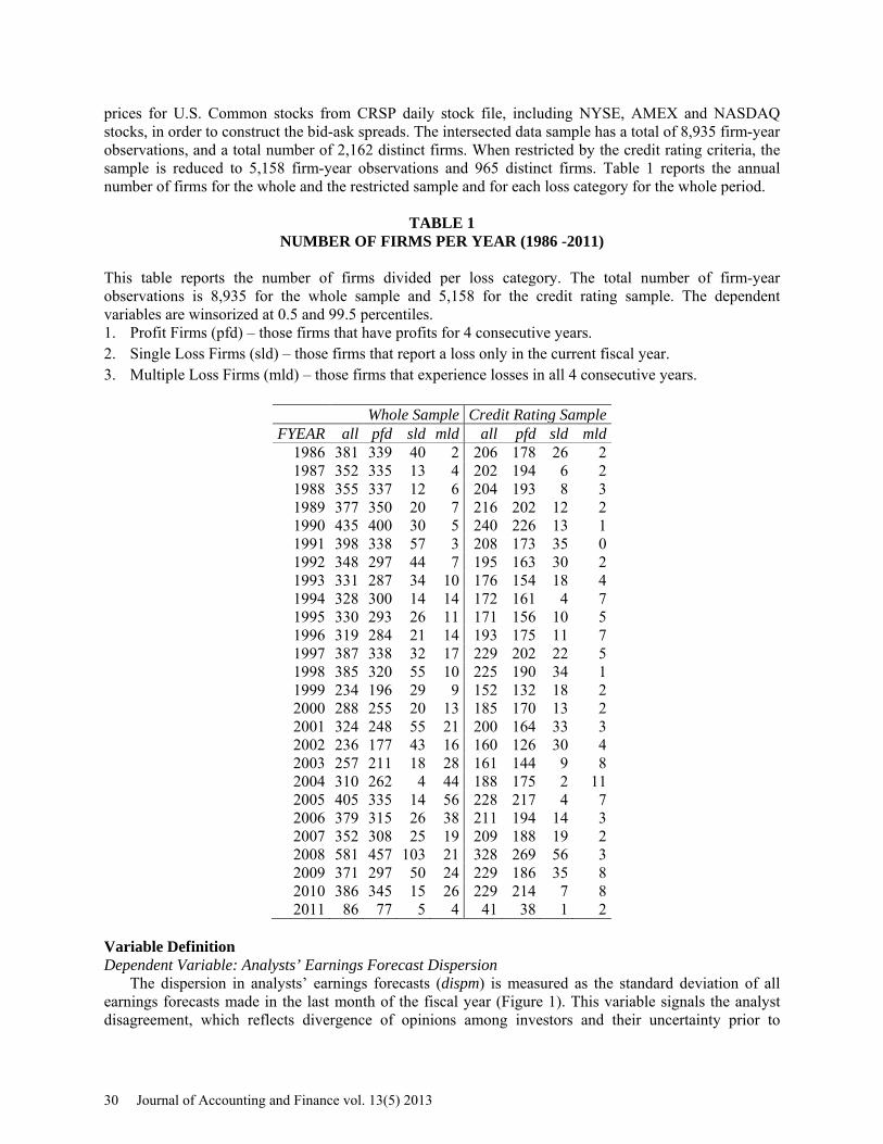
prices for U.S. Common stocks from CRSP daily stock file, including NYSE, AMEX and NASDAQ stocks, in order to construct the bid-ask spreads. The intersected data sample has a total of 8,935 firm-year observations, and a total number of 2,162 distinct firms. When restricted by the credit rating criteria, the sample is reduced to 5,158 firm-year observations and 965 distinct firms. Table 1 reports the annual number of firms for the whole and the restricted sample and for each loss category for the whole period.

TABLE 1 NUMBER OF FIRMS PER YEAR (1986 -2011)

This table reports the number of firms divided per loss category. The total number of firm-year observations is 8,935 for the whole sample and 5,158 for the credit rating sample. The dependent variables are winsorized at 0.5 and 99.5 percentiles. 1. Profit Firms (pfd) – those firms that have profits for 4 consecutive years. 2. Single Loss Firms (sld) – those firms that report a loss only in the current fiscal year. 3. Multiple Loss Firms (mld) – those firms that experience losses in all 4 consecutive years.

Whole Sample Credit Rating Sample FYEAR all pfd sld mld all pfd sld mld

1986 381 339 40 2 206 178 26 2 1987 352 335 13 4 202 194 6 2 1988 355 337 12 6 204 193 8 3 1989 377 350 20 7 216 202 12 2 1990 435 400 30 5 240 226 13 1 1991 398 338 57 3 208 173 35 0 1992 348 297 44 7 195 163 30 2 1993 331 287 34 10 176 154 18 4 1994 328 300 14 14 172 161 4 7 1995 330 293 26 11 171 156 10 5 1996 319 284 21 14 193 175 11 7 1997 387 338 32 17 229 202 22 5 1998 385 320 55 10 225 190 34 1 1999 234 196 29 9 152 132 18 2 2000 288 255 20 13 185 170 13 2 2001 324 248 55 21 200 164 33 3 2002 236 177 43 16 160 126 30 4 2003 257 211 18 28 161 144 9 8 2004 310 262 4 44 188 175 2 11 2005 405 335 14 56 228 217 4 7 2006 379 315 26 38 211 194 14 3 2007 352 308 25 19 209 188 19 2 2008 581 457 103 21 328 269 56 3 2009 371 297 50 24 229 186 35 8 2010 386 345 15 26 229 214 7 8 2011 86 77 5 4 41 38 1 2

Variable Definition Dependent Variable: Analysts’ Earnings Forecast Dispersion

The dispersion in analysts’ earnings forecasts (dispm) is measured as the standard deviation of all earnings forecasts made in the last month of the fiscal year (Figure 1). This variable signals the analyst disagreement, which reflects divergence of opinions among investors and their uncertainty prior to


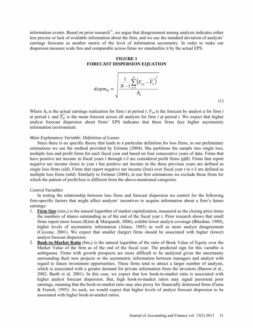
information events. Based on prior research11, we argue that disagreement among analysts indicates either less precise or lack of available information about the firm, and we use the standard deviation of analysts’ earnings forecasts as another metric of the level of information asymmetry. In order to make our dispersion measure scale free and comparable across firms we standardize it by the actual EPS.

FIGURE 1 FORECAST DISPERSION EQUATION

𝑑𝑖𝑠𝑝𝑚𝑖𝑡 =�

( )it

N

aitita

A

FFN

2

111 ∑

=

−−

(1) Where Ait is the actual earnings realization for firm i at period t; Fait is the forecast by analyst a for firm i at period t; and 𝐹𝚤𝑡�� is the mean forecast across all analysts for firm i at period t. We expect that higher analyst forecast dispersion about firms’ EPS indicates that these firms face higher asymmetric information environment. Main Explanatory Variable: Definition of Losses

Since there is no specific theory that leads to a particular definition for loss firms, in our preliminary estimations we use the method provided by Ertimur (2004). She partitions the sample into single loss, multiple loss and profit firms for each fiscal year end based on four consecutive years of data. Firms that have positive net income in fiscal years t through t-3 are considered profit firms (pfd). Firms that report negative net income (loss) in year t but positive net income in the three previous years are defined as single loss firms (sld). Firms that report negative net income (loss) over fiscal year t to t-3 are defined as multiple loss firms (mld). Similarly to Ertimur (2004), in our first estimations we exclude those firms for which the pattern of profit/loss is different from the above-mentioned categories. Control Variables

In testing the relationship between loss firms and forecast dispersion we control for the following firm-specific factors that might affect analysts’ incentives to acquire information about a firm’s future earnings: 1. Firm Size (sizeit) is the natural logarithm of market capitalization, measured as the closing price times

the numbers of shares outstanding as of the end of the fiscal year t. Prior research shows that small firms report more losses (Klein & Marquardt, 2006), exhibit lower analyst coverage (Bhushan, 1989), higher levels of asymmetric information (Atiase, 1985) as well as more analyst disagreement (Ciccone, 2001). We expect that smaller (larger) firms should be associated with higher (lower) analyst forecast dispersion.

2. Book-to-Market Ratio (bmit) is the natural logarithm of the ratio of Book Value of Equity over the Market Value of the firm as of the end of the fiscal year. The predicted sign for this variable is ambiguous. Firms with growth prospects are more difficult to be analyzed given the uncertainty surrounding their new projects or the asymmetric information between managers and analyst with regard to future investment opportunities. These firms tend to attract a larger number of analysts, which is associated with a greater demand for private information from the investors (Barron et al., 2002; Barth et al, 2001). In this case, we expect that low book-to-market ratio is associated with higher analyst forecast dispersion. But, high book-to-market ratios may signal persistent poor earnings, meaning that the book-to-market ratio may also proxy for financially distressed firms (Fama & French, 1995). As such, we would expect that higher levels of analyst forecast dispersion to be associated with higher book-to-market ratios.


3. Cash Flow Volatility (cfovolit) is measured as the rolling standard deviation of the operating cash flows–to–asset ratio for three consecutive years prior to fiscal year t. This variable controls for firm’s uncertainty12 (Ciccone, 2001), greater need from the analysts to acquire additional information in order to maintain the precision of their forecast (Barron et al., 1998) and reduces the bias in the measures of mean error analysts forecast (Lang & Lundholm, 1996). We would expect that higher levels of analyst forecast dispersion is associated with higher cash flow volatility.

4. Analyst Coverage (nanalit) is the number of analysts issuing one-year-ahead earnings’ forecasts in the last month of the fiscal year. Empirically, greater analyst coverage reduces the asymmetric information surrounding the firm whether it is represented by adverse selection risk (Brennan & Subrahmanyam, 1995) or forecast dispersion (Ciccone, 2001). If this is the case, we expect to find a negative association between the analyst coverage and analyst forecast dispersion in our estimations.

5. Forecast Error (errorfit) is measured as the absolute value of the difference between the actual and forecasted earnings per share, scaled by the actual earnings per share. The forecast error controls for measurement errors (Elton et al., 1984) or analyst optimism for more opaque and loss firms Controlling for this issue helps us distinguish whether financially distressed firms seem to be or truly are surrounded by poor information environments. Similar to the rest of the literature, we expect to find a positive association between forecast dispersion and forecast error.

Financial Distress Variables

In order to test for the second hypothesis, we make use of additional control variables that may proxy for the financial distress of the firms in our sample. 1. Credit Rating (arateit) is the categorical variable that indicates no financial distress. It is 1 if the

corporate bonds are rated as A+, A and A− in the last month prior to the ends of fiscal year and 0 otherwise. The bankruptcy literature categorizes a firm as financially distressed if it meets at least one of the following conditions: (1) defaults on its actual debt, (2) restructures the terms of debt instruments, (3) has difficulties to meet the payment requirements of debt contracts, or (4) its credit gets downgraded by the credit agencies (Avramov et al., 2009; Theodossiou et al., 1996). In our study we use the corporate bond rating proxied by the S&P Long-Term Domestic Issuer Credit Rating, which is available from COMPUSTAT on a monthly basis starting from May 1987. The majority of the firms in our sample have A-rated (A+, A-, A) and B-rated (B+, B-, B) debt. Given that only a handful of firms have C-and-D-rated debt and that we do not wish to lose any more observations from the sample, we choose to divide the sample into two groups of firms, those who have A-rated debt and those who don’t. We assume that firms with A-rated debt experience no financial distress, while the rest experience some financial distress. We expect that a downgrade of the corporate bond rating of a firm causes a higher dispersion in the analysts’ earnings forecasts.

2. Drop in Market Value (mvdropit) is a categorical variable that takes the value of 1 if the market value at the end of the fiscal year t has dropped compared to fiscal year t-1 and 0 otherwise. In his Z-score model, Altman (1968) uses the ratio of market value of equity to book value of liabilities as one of the factors that indicate financial distress. Campbell et al. (2010) use low stock prices as a proxy for the decline of the equity value of distressed firms. In our study, we use the drop in the market value of equity at year t as a possible indication that the company is experiencing financial difficulties. We expect that an increase in the incidence of drops of market value among firms will cause a higher dispersion in the level of analysts’ earnings forecasts.

3. Business Cycle (recessionit) is a categorical variable that equals one if the year is included in an NBER recession and zero otherwise. During the period 1986-2011 there were three NBER recession periods13 (Jul 1990 – Mar 1991; Mar 2001 – Nov 2001; and Dec 2007 – Jun 2009). Klein and Marquardt (2006) report a negative relation between the frequency of accounting losses and macroeconomic productivity. We expect that a recession event creates a more uncertain environment especially for the firms reporting losses, causing a higher dispersion in the analysts’ earnings forecasts. This variable is solely used in the Least Squares Regressions.


Bid-Ask Spread (basit) Corwin and Schultz (2012) develop a bid-ask spread estimator from daily high (ask) and low (bid)

prices, given the assumption that daily high (low) prices represent buy (sell) orders. Their high-low spread estimator is a function of high-low ratios over one-day and two-day intervals. In order to construct the bid-ask measure for our analysis, we take the average of high-low spread estimates from all overlapping two-day sub-periods within the test window. We also adjust for overnight price changes. Apart from being easy to construct and covering a period prior to 1992, the high-low spread estimator proposed by Corwin and Schultz (2012) is highly correlated to TAQ effective spreads (0.87 for monthly spreads and 0.75 for weekly spreads). Empirical Models

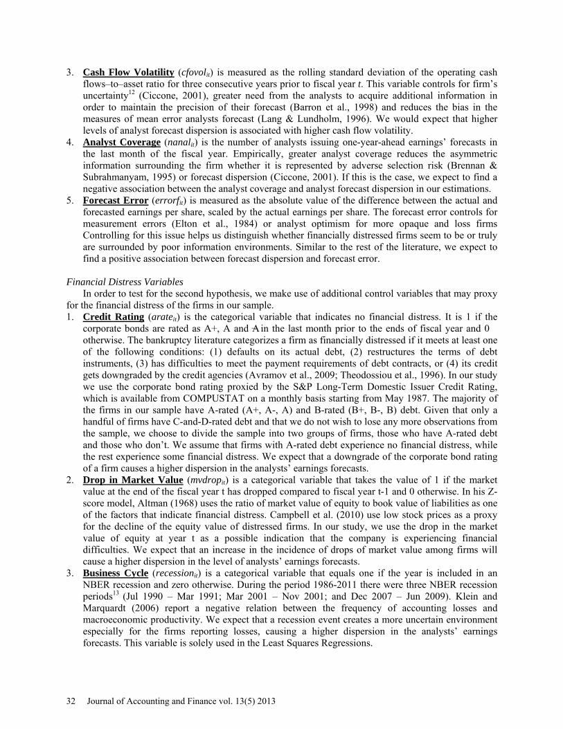
To investigate the effect of the loss incidence on the analyst earnings’ forecast dispersion (hypothesis 1), we first estimate the following regression:

FIGURE 2 MAIN REGRESSION EQUATION

titititi

titititititi

errorfcfovolnanalsizebmmldslddispm

,,7,6

,5,4,3,2,1,

εµαβββββββα

+++++

+++++=

(2)

Taking into consideration that this relationship may be driven by the financial distress, we extend the above equation by adding the financial distress variables to test the second hypothesis:

FIGURE 3 REGRESSION EQUATION CONTROLLING FOR FINANCIAL DISTRESS

tititititi

tititititititi

mvdroparateerrorfcfovolnanalsizebmmldslddispm

,,9,8,7

,6,5,4,3,2,1,

εµαβββββββββα

++++++

++++++=

(3)

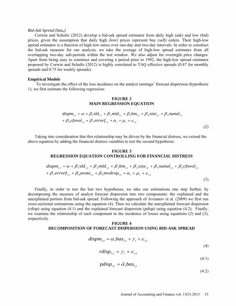
Finally, in order to test the last two hypotheses, we take our estimations one step further, by

decomposing the measure of analyst forecast dispersion into two components: the explained and the unexplained portion from bid-ask spread. Following the approach of Avramov et al. (2009) we first run cross-sectional estimations using the equation (4). Then we calculate the unexplained forecast dispersion (rdisp) using equation (4.1) and the explained forecast dispersion (pdisp) using equation (4.2). Finally, we examine the relationship of each component to the incidence of losses using equations (2) and (3), respectively.

FIGURE 4 DECOMPOSITION OF FORECAST DISPERSION USING BID-ASK SPREAD

tiititi basdispm ,,1, εγα ++=

(4)

tiitirdisp ,, εγ +=

(4.1)

titi baspdisp ,1, α̂=

(4.2)


We are ultimately interested on the impact of loss incidence on levels of asymmetric information, as captured by the level of analyst forecast dispersion. We perform tests using three different types of econometric frameworks: Least Squares, Fama-MacBeth and Panel Regressions. When we run panel regressions, we use a fixed effect estimator (αi) to focus on the within-dimension of the data. We also include time dummy variables (µt) to control for additional macroeconomic factors.

The coefficient estimates β1 and β2 capture the relationship between the analysts’ earnings forecast dispersion and single loss and multiple loss firms respectively, incremental to the relationship between the analysts’ earnings forecast dispersion and profit firms. In accordance with the stated hypotheses we expect β1>0 and β2>0.

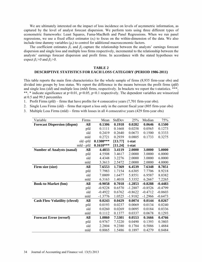
TABLE 2 DESCRIPTIVE STATISTICS FOR EACH LOSS CATEGORY (PERIOD 1986-2011)

This table reports the main firm characteristics for the whole sample of firms (8,935 firm-year obs) and divided into groups by loss status. We report the difference in the means between the profit firms (pfd) and single loss (sld) and multiple loss (mld) firms, respectively. In brackets we report the t-statistics. ***, **, * indicate significance at p<0.01, p<0.05, p<0.1 respectively. The dependent variables are winsorized at 0.5 and 99.5 percentiles 1. Profit Firms (pfd) – firms that have profits for 4 consecutive years (7,701 firm-year obs). 2. Single Loss Firms (sld) – firms that report a loss only in the current fiscal year (805 firm-year obs) 3. Multiple Loss Firms (mld) – firms with losses in all 4 consecutive years (429 firm-year obs)

Variable Firms Mean StdDev 25% Median 75% Forecast Dispersion (dispm) All 0.1306 0.1918 0.0282 0.0646 0.1500 pfd 0.1111 0.1668 0.0258 0.0565 0.1273 sld 0.2419 0.2640 0.0673 0.1500 0.3333 mld 0.2721 0.2939 0.0805 0.1733 0.3275

sld -pfd 0.1308*** [13.77] t-stat mld - pfd 0.1610*** [11.24] t-stat

Number of Analysts (nanal) All 4.4833 3.4119 2.0000 3.0000 5.0000 pfd 4.5508 3.4617 2.0000 3.0000 6.0000 sld 4.4348 3.2276 2.0000 3.0000 6.0000 mld 3.3613 2.5472 2.0000 2.0000 4.0000 Firm size (size) All 7.6553 1.7369 6.4539 7.6348 8.7851 pfd 7.7983 1.7154 6.6305 7.7706 8.9218 sld 7.0009 1.6477 5.8551 6.9587 8.0382 mld 6.3163 1.4018 5.3352 6.2667 7.2265 Book-to-Market (bm) All -0.9058 0.7018 -1.2853 -0.8288 -0.4483 pfd -0.9228 0.6570 -1.2887 -0.8526 -0.4799 sld -0.4922 0.6762 -0.8622 -0.4712 -0.0603 mld -1.3776 1.0525 -1.9182 -1.2966 -0.6473 Cash Flow Volatility (cfovol) All 0.0243 0.0429 0.0074 0.0144 0.0267 pfd 0.0193 0.0237 0.0069 0.0134 0.0240 sld 0.0260 0.0269 0.0095 0.0184 0.0336 mld 0.1112 0.1377 0.0337 0.0678 0.1293 Forecast Error (errorf) All 1.0860 7.5301 0.0553 0.1666 0.4766 pfd 0.9767 7.5220 0.0490 0.1393 0.3803 sld 2.2804 9.2380 0.1784 0.5886 1.4884 mld 0.8065 1.5486 0.1897 0.4279 0.8484


EMPIRICAL RESULTS Summary Statistics

We report the summary statistics for the whole sample and for each loss category in Table 2. The period covered is from 1986 to 2011. The distribution for the level of analyst forecast dispersion is highly skewed. The mean (median) of the level of analyst forecast dispersion is 0.13 (0.07). The mean (median) of the level of the forecast dispersion increases monotonically as from profit to loss firms, confirming our expectations that the analyst disagreement is higher for firms experiencing losses relative to profit firms. The t-test procedure further confirms that the average forecast dispersion is statistically different for profit firms and single loss and multiple loss firms respectively.

As expected, we report a monotonic decrease in firm size and monotonic increase in the cash flow volatility as we switch from profit firms to single loss to multiple loss firms. But, we observe a non-monotonic behavior for the average book-to-market ratio, which is highest (as expected) for multiple loss firms but the lowest (unexpected) for single loss firms. The average number of analysts that follow the firm by the end of the fiscal year is 4.5. But, differently from our expectations, we report a monotonic decrease in the mean analyst coverage from profit firms to multiple loss firms. Finally, as expected, the forecast error seems to be higher for single loss firms relative to profit firms, but unexpectedly it is lower for multiple loss firms relative to the other groups.

Although the size of the credit rating sample14 is smaller compared to the unrestricted sample, the variables behave similarly. In the credit rating sample the majority of the observations include firms that have A-rated debts (2,570 firm-year observations) or B-rated debt (2,567 firm-year observations) as compared to only 20 firm-year observations with C/D-rated debt. The average level of forecast dispersion is highest for C/D-rated debt (0.2376), compared to both B-rated (0.1709) and A-rated debt firms (0.0929). Similarly, the average level of forecast dispersion is highest for the group of firms that experienced a drop in the market value in the current year, 0.1717 versus 0.1063 for the group of firms that do not experience a drop in the market value in the current year. Analyst Forecast Dispersion and Loss Incidence

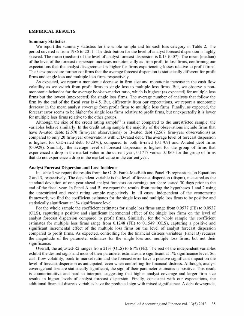
In Table 3 we report the results from the OLS, Fama-MacBeth and Panel FE regressions on Equations 2 and 3, respectively. The dependent variable is the level of forecast dispersion (dispm), measured as the standard deviation of one-year-ahead analyst forecasts on earnings per share issued 30 days prior to the end of the fiscal year. In Panel A and B, we report the results from testing the hypotheses 1 and 2 using the unrestricted and credit rating sample respectively. In all cases, independent of the econometric framework, we find the coefficient estimates for the single loss and multiple loss firms to be positive and statistically significant at 1% significance level.

For the whole sample the coefficient estimates for single loss firms range from 0.0577 (FE) to 0.0937 (OLS), capturing a positive and significant incremental effect of the single loss firms on the level of analyst forecast dispersion compared to profit firms. Similarly, for the whole sample the coefficient estimates for multiple loss firms range from 0.1248 (FE) to 0.1549 (OLS), capturing a positive and significant incremental effect of the multiple loss firms on the level of analyst forecast dispersion compared to profit firms. As expected, controlling for the financial distress variables (Panel B) reduces the magnitude of the parameter estimates for the single loss and multiple loss firms, but not their significance.

Overall, the adjusted-R2 ranges from 21% (OLS) to 61% (FE). The rest of the independent variables exhibit the desired signs and most of their parameter estimates are significant at 1% significance level. So, cash flow volatility, book-to-market ratio and the forecast error have a positive significant impact on the level of forecast dispersion as anticipated, even when controlling for financial distress. Although, analyst coverage and size are statistically significant, the sign of their parameter estimates is positive. This result is counterintuitive and hard to interpret, suggesting that higher analyst coverage and larger firm size results in higher levels of analyst forecast dispersion. Finally, consistent with our expectations, the additional financial distress variables have the predicted sign with mixed significance. A debt downgrade,


a drop in current market value and the occurrence of a recession result in a significant increase of forecast dispersion. Our findings are supportive of both hypotheses 1 and 2.

TABLE 3 ESTIMATED IMPACT OF LOSS INCIDENCE ON ANALYST FORECAST DISPERSION

This table shows the estimation results when we run OLS, Fama-MacBeth and Panel FE regressions based on the Equations 2 and 3. The dependent variable in all specifications is the level of the dispersion of one-year-ahead analyst EPS forecasts issued 30 days before the end of the fiscal year. We report the results for both the whole sample (8,935 observations) and credit rated sample (5,158). The sample period is 1986-2011. The adjusted-R2 of the fixed effects regression refers to the overall fit. The adjusted-R2 for the Fama-MacBeth regression is the average value of the R2-s of the single years. In brackets we show the t-stats. ***, **, * indicate significance at p<0.01, p<0.05, p<0.1 respectively. Standard errors and t-statistics for Fama-MacBeth estimations are adjusted for autocorrelation using Newey-West (1987) and 3 lags.

A: Whole Sample B: Credit Rating Sample

Parameter Predicted Sign OLS

Fama-MacBeth

Fixed Effects OLS

Fama-MacBeth

Fixed Effects

Intercept 0.1240*** 0.0999*** 0.1200*** 0.0586** (14.01) (8.96) (8.02) (2.45)

sld + 0.0937*** 0.0772*** 0.0577*** 0.0729*** 0.0514*** 0.0459*** (14.49) (7.40) (8.74) (8.50) (5.11) (5.55)

mld + 0.1549*** 0.1772*** 0.1258*** 0.1398*** 0.1923*** 0.1062*** (15.95) (6.44) (6.45) (7.90) (4.14) (3.89)

bm -/+ 0.0593*** 0.0518*** 0.0386*** 0.0573*** 0.0499*** 0.0382*** (20.40) (7.94) (8.56) (14.12) (6.57) (6.50)

size - -0.0010 -0.0001 0.0170*** -0.0006 0.0042 0.0233*** (-0.80) (-0.08) (4.49) (-0.30) (1.55) (4.23)

nanal - 0.0076*** 0.0063*** 0.0047*** 0.0071*** 0.0047*** 0.0039*** (13.17) (8.48) (8.13) (10.41) (9.45) (5.76)

cfovol + 0.4538*** 0.5593*** 0.1892** 1.0613*** 1.4004*** 0.2605** (9.42) (5.41) (2.40) (9.88) (6.07) (2.25)

errorf + 0.0066*** 0.0206*** 0.0066*** 0.0057*** 0.0360*** 0.0063***

(27.36) (5.67) (28.23) (18.14) (5.55) (20.79) arate -

-0.0368*** -0.0268*** -0.0105

(-6.90) (-4.03) (-1.30) mvdrop +

0.0222*** 0.0140*** 0.0177***

(4.33) (2.95) (3.46) recession +

0.0277***

(4.80)

Adj-R2 0.205 0.331 0.6098 0.2195 0.4134 0.5591 Obs 8,935 8,935 8,935 5,158 5,158 5,158 Years 26 26 26 26 26 26 Firms 2,162 2,162 2,162 965 965 965 Forecast Dispersion and Loss Incidence: Uncertainty vs. Asymmetric Information

In this section we test hypotheses 3 and 4. Theoretically, analyst forecast dispersion may be used as a proxy for both uncertainty and information asymmetry. We argue that if we separate the forecast


dispersion based on its relationship to bid-ask spread, we are able to isolate the component that is more prone to represent the asymmetric effect (the predicted dispersion from bid-ask spread) and the component that is more prone to represent uncertainty (the residuals plus the fixed effects from the regression). First, we run estimations of the analyst forecast dispersion on the bid-ask spreads using equation 4, and then construct the above components using equations 4.1 and 4.2. Both components are used as dependent variables to test for the last two hypotheses, running regressions on equations 2 and 3. One limitation is that since bid-ask spread is not pure asymmetric information measure15 both components may not represent pure effects.

Following Ertimur (2004), we construct our sample of bid-ask spreads, the level of analyst forecast dispersion and other financial data, over a window starting 7 days after the annual earnings announcement for fiscal year t and ending 7 days before the first quarterly earnings announcement of fiscal year t+1. Ertimur (2004) argues that this test window provides a reasonable compromise over very short or very long testing periods. If the test window surrounding the earnings announcements is too short, then we may capture an increase in information asymmetry due to anticipation in public disclosure. On the other hand, if the test window is too long, say annually, the perceived loss status of the firm changes as quarterly earnings information becomes available, reducing the power of estimations. Similarly to Ertimur (2004), we also exclude firms that trade at an average price less than $1 and those that have fewer than five days of price data during the test window, in order to avoid highly illiquid stocks. However, she uses Transactions and Quotes (TAQ) database, while our measure of bid-ask spread is constructed entirely using data from CRSP daily stock data from WRDS based on the approach described by Corwin and Schultz (2012).

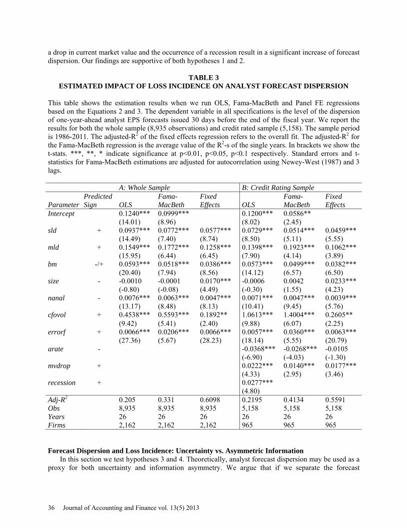
Given the new selection criteria the total number of firm-year observations changes to 12,291 and 6,741 for the whole and credit rating sample respectively. The datasets cover the period from 1985 to 2010. We find a significant positive correlation between the forecast dispersion (dispm) and the high-low spread estimator (bas) of 19% for the whole sample and 21% for the credit rating sample. The rest of the firm characteristics behave in similar fashion as for the end of fiscal year sample16.

TABLE 4

PANEL REGRESSION: DECOMPOSITION OF FORECAST DISPERSION USING BID-ASK SPREAD

This table reports the estimation results when we run panel regressions with firm fixed effects using Equation 4. The dependent variable in all specifications is the level of the dispersion (dispm) on forecasts issued over a window starting 7 days after the annual earnings announcement for fiscal year t and ending 7 days before the first quarterly earnings announcement of fiscal year t+1. The independent variable is the bid-ask spread (bas) calculated during the same period using the approach from Corwin and Schultz (2012). We report the results for both the whole sample (12,291 observations) and credit rated sample (6,741). The datasets cover the period 1985-2010. The adjusted-R2 of the fixed effects regression refers to the overall fit. In brackets we show the t-stats. ***, **, * indicate significance at p<0.01, p<0.05, p<0.1 respectively.

Whole Sample Credit Rating Sample

Parameter Predicted Sign dispm dispm

bas + 6.2134*** 8.1822*** (12.26) (11.24)

Adj R2 0.5141 0.5396 Obs 12,291 6,741 Firms 2,265 973


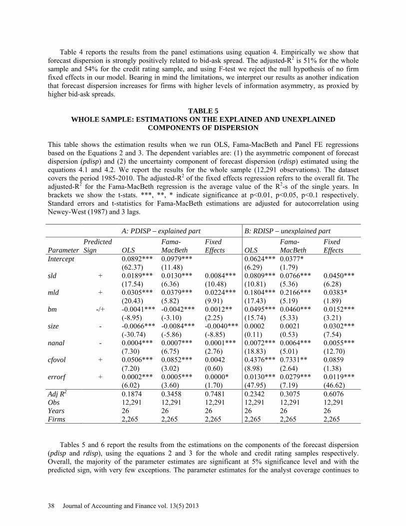
Table 4 reports the results from the panel estimations using equation 4. Empirically we show that forecast dispersion is strongly positively related to bid-ask spread. The adjusted-R2 is 51% for the whole sample and 54% for the credit rating sample, and using F-test we reject the null hypothesis of no firm fixed effects in our model. Bearing in mind the limitations, we interpret our results as another indication that forecast dispersion increases for firms with higher levels of information asymmetry, as proxied by higher bid-ask spreads.

TABLE 5

WHOLE SAMPLE: ESTIMATIONS ON THE EXPLAINED AND UNEXPLAINED COMPONENTS OF DISPERSION

This table shows the estimation results when we run OLS, Fama-MacBeth and Panel FE regressions based on the Equations 2 and 3. The dependent variables are: (1) the asymmetric component of forecast dispersion (pdisp) and (2) the uncertainty component of forecast dispersion (rdisp) estimated using the equations 4.1 and 4.2. We report the results for the whole sample (12,291 observations). The dataset covers the period 1985-2010. The adjusted-R2 of the fixed effects regression refers to the overall fit. The adjusted-R2 for the Fama-MacBeth regression is the average value of the R2-s of the single years. In brackets we show the t-stats. ***, **, * indicate significance at p<0.01, p<0.05, p<0.1 respectively. Standard errors and t-statistics for Fama-MacBeth estimations are adjusted for autocorrelation using Newey-West (1987) and 3 lags.

A: PDISP – explained part B: RDISP – unexplained part


Fama-MacBeth

Fixed Effects OLS

Fama-MacBeth

Fixed Effects

Intercept 0.0892*** 0.0979*** 0.0624*** 0.0377* (62.37) (11.48) (6.29) (1.79)

sld + 0.0189*** 0.0130*** 0.0084*** 0.0809*** 0.0766*** 0.0450*** (17.54) (6.36) (10.48) (10.81) (5.36) (6.28)

mld + 0.0305*** 0.0379*** 0.0224*** 0.1804*** 0.2166*** 0.0383* (20.43) (5.82) (9.91) (17.43) (5.19) (1.89)

bm -/+ -0.0041*** -0.0042*** 0.0012** 0.0495*** 0.0460*** 0.0152*** (-8.95) (-3.10) (2.25) (15.74) (5.33) (3.21)

size - -0.0066*** -0.0084*** -0.0040*** 0.0002 0.0021 0.0302*** (-30.74) (-5.86) (-8.85) (0.11) (0.53) (7.54)

nanal - 0.0004*** 0.0007*** 0.0001*** 0.0072*** 0.0064*** 0.0055*** (7.30) (6.75) (2.76) (18.83) (5.01) (12.70)

cfovol + 0.0506*** 0.0852*** 0.0042 0.4376*** 0.7331** 0.0859 (7.20) (3.02) (0.60) (8.98) (2.64) (1.38)

errorf + 0.0002*** 0.0005*** 0.0000* 0.0130*** 0.0279*** 0.0119***

(6.02) (3.60) (1.70) (47.95) (7.19) (46.62) Adj R2 0.1874 0.3458 0.7481 0.2342 0.3075 0.6076 Obs 12,291 12,291 12,291 12,291 12,291 12,291 Years 26 26 26 26 26 26 Firms 2,265 2,265 2,265 2,265 2,265 2,265

Tables 5 and 6 report the results from the estimations on the components of the forecast dispersion (pdisp and rdisp), using the equations 2 and 3 for the whole and credit rating samples respectively. Overall, the majority of the parameter estimates are significant at 5% significance level and with the predicted sign, with very few exceptions. The parameter estimates for the analyst coverage continues to


be significantly positive. In almost all cases, whether the dependent variable is the explained (pdsip) or unexplained (rdisp) forecast dispersion by bid-ask spread, the parameter estimates on the single loss firms (sld) and multiple loss firms (mld) are positive and significant. These results indicate that the loss incidence can explain both the uncertainty and the asymmetric information surrounding the firm, providing further support for the last two hypotheses.

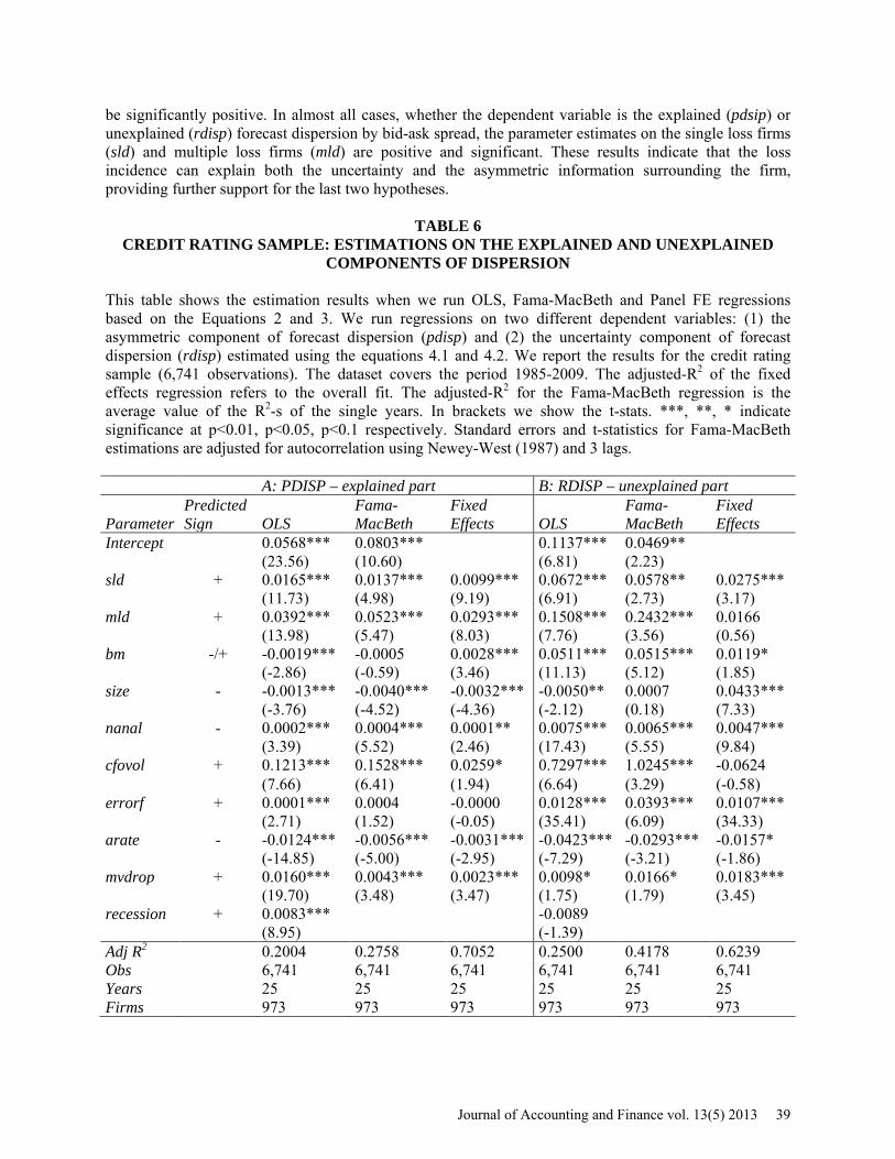
TABLE 6 CREDIT RATING SAMPLE: ESTIMATIONS ON THE EXPLAINED AND UNEXPLAINED

COMPONENTS OF DISPERSION

This table shows the estimation results when we run OLS, Fama-MacBeth and Panel FE regressions based on the Equations 2 and 3. We run regressions on two different dependent variables: (1) the asymmetric component of forecast dispersion (pdisp) and (2) the uncertainty component of forecast dispersion (rdisp) estimated using the equations 4.1 and 4.2. We report the results for the credit rating sample (6,741 observations). The dataset covers the period 1985-2009. The adjusted-R2 of the fixed effects regression refers to the overall fit. The adjusted-R2 for the Fama-MacBeth regression is the average value of the R2-s of the single years. In brackets we show the t-stats. ***, **, * indicate significance at p<0.01, p<0.05, p<0.1 respectively. Standard errors and t-statistics for Fama-MacBeth estimations are adjusted for autocorrelation using Newey-West (1987) and 3 lags.

A: PDISP – explained part B: RDISP – unexplained part


Fama-MacBeth

Fixed Effects OLS

Fama-MacBeth

Fixed Effects

Intercept 0.0568*** 0.0803*** 0.1137*** 0.0469** (23.56) (10.60) (6.81) (2.23)

sld + 0.0165*** 0.0137*** 0.0099*** 0.0672*** 0.0578** 0.0275*** (11.73) (4.98) (9.19) (6.91) (2.73) (3.17)

mld + 0.0392*** 0.0523*** 0.0293*** 0.1508*** 0.2432*** 0.0166 (13.98) (5.47) (8.03) (7.76) (3.56) (0.56)

bm -/+ -0.0019*** -0.0005 0.0028*** 0.0511*** 0.0515*** 0.0119* (-2.86) (-0.59) (3.46) (11.13) (5.12) (1.85)

size - -0.0013*** -0.0040*** -0.0032*** -0.0050** 0.0007 0.0433*** (-3.76) (-4.52) (-4.36) (-2.12) (0.18) (7.33)

nanal - 0.0002*** 0.0004*** 0.0001** 0.0075*** 0.0065*** 0.0047*** (3.39) (5.52) (2.46) (17.43) (5.55) (9.84)

cfovol + 0.1213*** 0.1528*** 0.0259* 0.7297*** 1.0245*** -0.0624 (7.66) (6.41) (1.94) (6.64) (3.29) (-0.58)

errorf + 0.0001*** 0.0004 -0.0000 0.0128*** 0.0393*** 0.0107***

(2.71) (1.52) (-0.05) (35.41) (6.09) (34.33) arate - -0.0124*** -0.0056*** -0.0031*** -0.0423*** -0.0293*** -0.0157*

(-14.85) (-5.00) (-2.95) (-7.29) (-3.21) (-1.86) mvdrop + 0.0160*** 0.0043*** 0.0023*** 0.0098* 0.0166* 0.0183***

(19.70) (3.48) (3.47) (1.75) (1.79) (3.45) recession + 0.0083*** -0.0089

(8.95) (-1.39)

Adj R2 0.2004 0.2758 0.7052 0.2500 0.4178 0.6239 Obs 6,741 6,741 6,741 6,741 6,741 6,741 Years 25 25 25 25 25 25 Firms 973 973 973 973 973 973


So, the decomposition of the analyst forecast dispersion into two components based on the bid-ask spread, provides a possible reconciliation in the different results provided in Ertimur (2004) and Ciccone (2001) about the incidence of losses. Yet, the larger coefficient estimates for both single and multiple loss firms in the regressions for the unexplained portion of analyst forecast dispersion (rdisp) compared to those for the explained portion of analyst forecast dispersion (pdisp), may further indicate that the incidence of losses, empirically, captures more easily the uncertainty surrounding the firms. ROBUSTNESS CHECKS

To further ascertain the positive relationship that we have documented between the earnings’ analyst forecast dispersion and the loss incidence we employ additional regression tests to demonstrate robustness. However, in order not to overcrowd the paper with similar tables we only report the parameter estimates for the most conservative model: panel fixed effects regressions on the credit rating sample (refer to Table 8)17. Change in Analyst Forecast Dispersion

Barron et al. (2009) use the theoretical framework of Barron et al. (1998) to separate the dispersion into two theoretical components: uncertainty and information asymmetry. They argue that the level of dispersion prior to earnings announcements reflects uncertainty, while the change in dispersion reflects information asymmetry. Similarly to Barron et al. (2009), we test hypotheses 1 and 2 using the change in the forecast dispersion as the dependent variable. To be included in the change sample, 2 or more individual analysts must have issued forecasts both within a 30-day pre-and post-announcement window. Different analysts are allowed to issue forecasts in both pre- and post-announcement windows. In the calculation of the forecast dispersion we take into account the total number of forecasts during the 30-day period (nanal). We construct three measures for the level of forecast dispersion: (1) bdispm – the level of forecast dispersion 30 days prior to the 4th quarter earnings announcement; (2) adispm – the level of forecast dispersion 30 days after the 4th quarter earnings announcement; and (3) ddispm – the change in the level of forecast dispersion found as the difference between adispm and bdispm. In similar fashion we construct the respective versions for the number of forecasts and the forecast error.

Empirical literature suggests that uncertainty is most likely to decline following public disclosure around earnings announcements, but the impact on the information asymmetry is ambiguous. Kim and Verrecchia (1997) develop a theoretical model where they suggest that investors develop new private information in response to earnings announcement, resulting in higher information asymmetry. Barron et al. (2005) find supporting evidence by documenting an increase in the abnormal trading volume, used as a proxy for asymmetric information, around earnings announcement. On the contrary, Botosan and Stanford (2005) find that higher disclosure is associated with a decline in information asymmetry, measured by the consensus of analysts developed by Barron et al (1998). We assume that once, the earnings are announced and the status of the firm is realized, this should have a dissipating effect at least on uncertainty. In the case, it is more likely that the forecast dispersion measured after the earnings announcement proxies mainly for asymmetric information. Given the ambiguous empirical evidence on asymmetric information, we do not make any predictions on the direction after the earnings announcement, but let the data speak for itself.

After applying the new selection criteria the total number of firm-year observations changes to 7,381 and 4,427 for the whole and credit rating sample respectively. The datasets cover the period from 1989 to 2010. In order not to overcrowd the paper with similar tables, we report in Table 7 the most conservative results from the panel regression estimations with fixed effects using the three variables that we construct in this section. For both samples we find that our model works well in explaining the level of forecast dispersion 30-days prior to (bdispm) and 30-days after (adispm) the 4th quarter earnings announcements. A higher number of single loss and/or multiple loss firms results in increased levels of forecast dispersion before and after the 4th quarter earnings announcements. However, the results from Table 7 show that our model is not successful in explaining the change in forecast dispersion (ddispm). So, when we use the


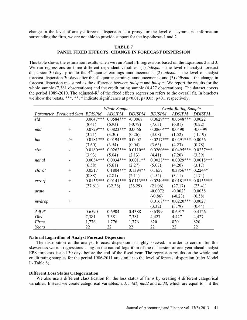
change in the level of analyst forecast dispersion as a proxy for the level of asymmetric information surrounding the firm, we are not able to provide support for the hypotheses 1 and 2.

TABLE 7 PANEL FIXED EFFECTS: CHANGE IN FORECAST DISPERSION

This table shows the estimation results when we run Panel FE regressions based on the Equations 2 and 3. We run regressions on three different dependent variables: (1) bdispm – the level of analyst forecast dispersion 30-days prior to the 4th quarter earnings announcements; (2) adispm – the level of analyst forecast dispersion 30-days after the 4th quarter earnings announcements; and (3) ddispm – the change in forecast dispersion measured as the difference between adispm and bdispm. We report the results for the whole sample (7,381 observations) and the credit rating sample (4,427 observations). The dataset covers the period 1989-2010. The adjusted-R2 of the fixed effects regression refers to the overall fit. In brackets we show the t-stats. ***, **, * indicate significance at p<0.01, p<0.05, p<0.1 respectively.

Whole Sample Credit Rating Sample Parameter Predicted Sign BDISPM ADSIPM DDISPM BDISPM ADSIPM DDISPM sld + 0.0647*** 0.0584*** -0.0068 0.0629*** 0.0648*** 0.0022

(8.41) (6.93) (-0.79) (7.63) (6.81) (0.22) mld + 0.0729*** 0.0823*** 0.0066 0.0860*** 0.0490 -0.0399

(3.21) (3.30) (0.26) (3.08) (1.52) (-1.19) bm -/+ 0.0181*** 0.0194*** 0.0002 0.0217*** 0.0291*** 0.0056

(3.60) (3.54) (0.04) (3.63) (4.23) (0.78) size - 0.0180*** 0.0262*** 0.0110** 0.0260*** 0.0495*** 0.0237***

(3.93) (5.04) (2.13) (4.41) (7.20) (3.39) nanal - 0.0034*** 0.0034*** 0.0011** 0.0028*** 0.0029*** 0.0018***

(6.58) (5.61) (2.27) (5.07) (4.20) (3.17) cfovol + 0.0517 0.1804*** 0.1394** 0.1657 0.3856*** 0.2244*

(0.88) (2.81) (2.11) (1.54) (3.11) (1.74) errorf + 0.0155*** 0.0141*** 0.0113*** 0.0249*** 0.0181*** 0.0155***

(27.61) (32.36) (26.29) (21.06) (27.17) (23.41) arate -

-0.0072 -0.0023 0.0058

(-0.86) (-0.23) (0.58) mvdrop + 0.0168*** 0.0220*** 0.0027

(3.32) (3.79) (0.44) Adj R2 0.6590 0.6904 0.4388 0.6399 0.6917 0.4126 Obs 7,381 7,381 7,381 4,427 4,427 4,427 Firms 1,776 1,776 1,776 820 820 820 Years 22 22 22 22 22 22

Natural Logarithm of Analyst Forecast Dispersion

The distribution of the analyst forecast dispersion is highly skewed. In order to control for this skeweness we run regressions using on the natural logarithm of the dispersion of one-year-ahead analyst EPS forecasts issued 30 days before the end of the fiscal year. The regression results on the whole and credit rating samples for the period 1986-2011 are similar to the level of forecast dispersion (refer Model I - Table 8). Different Loss Status Categorization

We also use a different classification for the loss status of firms by creating 4 different categorical variables. Instead we create categorical variables: sld, mld1, mld2 and mld3, which are equal to 1 if the


firm only experiences a loss in the year t, t-1, t-2 or t-3 respectively, and 0 otherwise. In almost all the estimations we find positive significant coefficient estimates associated with the loss categorical variables associated with the current loss (sld), and lagged losses up to two years (mld1 and mld2). However, in most of the regressions the parameter estimates for the categorical variable mld3, associated with losses occurring in the fiscal year t-3, is not statistically different from 0 and sometimes exhibits the wrong sign (refer to the parameter estimates for Model II - Table 8).

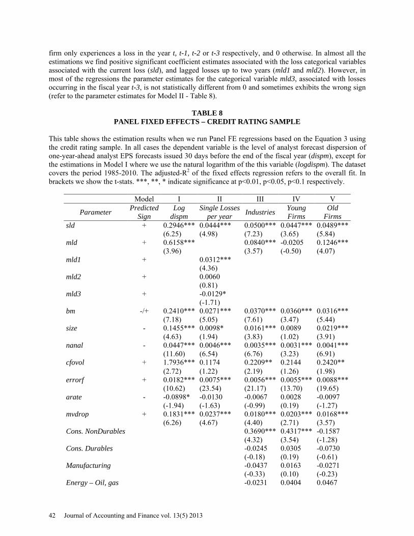
TABLE 8 PANEL FIXED EFFECTS – CREDIT RATING SAMPLE

This table shows the estimation results when we run Panel FE regressions based on the Equation 3 using the credit rating sample. In all cases the dependent variable is the level of analyst forecast dispersion of one-year-ahead analyst EPS forecasts issued 30 days before the end of the fiscal year (dispm), except for the estimations in Model I where we use the natural logarithm of the this variable (logdispm). The dataset covers the period 1985-2010. The adjusted-R2 of the fixed effects regression refers to the overall fit. In brackets we show the t-stats. ***, **, * indicate significance at p<0.01, p<0.05, p<0.1 respectively.

Model I II III IV V

Parameter Predicted Sign

Log dispm

Single Losses per year Industries Young

Firms Old

Firms sld + 0.2946*** 0.0444*** 0.0500*** 0.0447*** 0.0489***

(6.25) (4.98) (7.23) (3.65) (5.84) mld + 0.6158*** 0.0840*** -0.0205 0.1246***

(3.96) (3.57) (-0.50) (4.07) mld1 + 0.0312*** (4.36) mld2 + 0.0060 (0.81) mld3 + -0.0129* (-1.71) bm -/+ 0.2410*** 0.0271*** 0.0370*** 0.0360*** 0.0316***

(7.18) (5.05) (7.61) (3.47) (5.44) size - 0.1455*** 0.0098* 0.0161*** 0.0089 0.0219***

(4.63) (1.94) (3.83) (1.02) (3.91) nanal - 0.0447*** 0.0046*** 0.0035*** 0.0031*** 0.0041***

(11.60) (6.54) (6.76) (3.23) (6.91) cfovol + 1.7936*** 0.1174 0.2209** 0.2144 0.2420**

(2.72) (1.22) (2.19) (1.26) (1.98) errorf + 0.0182*** 0.0075*** 0.0056*** 0.0055*** 0.0088***

(10.62) (23.54) (21.17) (13.70) (19.65) arate - -0.0898* -0.0130 -0.0067 0.0028 -0.0097

(-1.94) (-1.63) (-0.99) (0.19) (-1.27) mvdrop + 0.1831*** 0.0237*** 0.0180*** 0.0203*** 0.0168***

(6.26) (4.67) (4.40) (2.71) (3.57) Cons. NonDurables 0.3690*** 0.4317*** -0.1587

(4.32) (3.54) (-1.28) Cons. Durables -0.0245 0.0305 -0.0730

(-0.18) (0.19) (-0.61) Manufacturing -0.0437 0.0163 -0.0271

(-0.33) (0.10) (-0.23) Energy – Oil, gas -0.0231 0.0404 0.0467


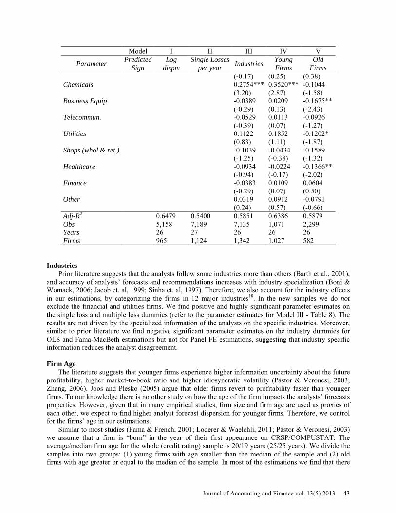
Model I II III IV V

Parameter Predicted Sign

Log dispm

Single Losses per year Industries Young

Firms Old

Firms

(-0.17) (0.25) (0.38) Chemicals 0.2754*** 0.3520*** -0.1044

(3.20) (2.87) (-1.58) Business Equip -0.0389 0.0209 -0.1675**

(-0.29) (0.13) (-2.43) Telecommun. -0.0529 0.0113 -0.0926

(-0.39) (0.07) (-1.27) Utilities 0.1122 0.1852 -0.1202*

(0.83) (1.11) (-1.87) Shops (whol.& ret.) -0.1039 -0.0434 -0.1589

(-1.25) (-0.38) (-1.32) Healthcare -0.0934 -0.0224 -0.1366**

(-0.94) (-0.17) (-2.02) Finance -0.0383 0.0109 0.0604

(-0.29) (0.07) (0.50) Other 0.0319 0.0912 -0.0791

(0.24) (0.57) (-0.66) Adj-R2 0.6479 0.5400 0.5851 0.6386 0.5879 Obs 5,158 7,189 7,135 1,071 2,299 Years 26 27 26 26 26 Firms 965 1,124 1,342 1,027 582

Industries

Prior literature suggests that the analysts follow some industries more than others (Barth et al., 2001), and accuracy of analysts’ forecasts and recommendations increases with industry specialization (Boni & Womack, 2006; Jacob et. al, 1999; Sinha et. al, 1997). Therefore, we also account for the industry effects in our estimations, by categorizing the firms in 12 major industries18. In the new samples we do not exclude the financial and utilities firms. We find positive and highly significant parameter estimates on the single loss and multiple loss dummies (refer to the parameter estimates for Model III - Table 8). The results are not driven by the specialized information of the analysts on the specific industries. Moreover, similar to prior literature we find negative significant parameter estimates on the industry dummies for OLS and Fama-MacBeth estimations but not for Panel FE estimations, suggesting that industry specific information reduces the analyst disagreement. Firm Age

The literature suggests that younger firms experience higher information uncertainty about the future profitability, higher market-to-book ratio and higher idiosyncratic volatility (Pástor & Veronesi, 2003; Zhang, 2006). Joos and Plesko (2005) argue that older firms revert to profitability faster than younger firms. To our knowledge there is no other study on how the age of the firm impacts the analysts’ forecasts properties. However, given that in many empirical studies, firm size and firm age are used as proxies of each other, we expect to find higher analyst forecast dispersion for younger firms. Therefore, we control for the firms’ age in our estimations.

Similar to most studies (Fama & French, 2001; Loderer & Waelchli, 2011; Pástor & Veronesi, 2003) we assume that a firm is “born” in the year of their first appearance on CRSP/COMPUSTAT. The average/median firm age for the whole (credit rating) sample is 20/19 years (25/25 years). We divide the samples into two groups: (1) young firms with age smaller than the median of the sample and (2) old firms with age greater or equal to the median of the sample. In most of the estimations we find that there


is a positive significant relationship between the analyst forecast dispersion and the loss incidence, supporting our hypotheses (refer to parameter estimates in Models IV and V – Table 8). This positive relationship is driven by both, the asymmetric and uncertainty components of forecast dispersion. CONCLUSION

In this study we examine whether the firms that report losses experience higher levels of information

asymmetry among investors relative to firms that report profits. We use the dispersion in analysts’ earnings forecasts as a proxy for the level of information asymmetry among the investors. Prior research documents mixed evidence on the relationship of incidence of losses and levels of asymmetric information, mainly due to the fact that empirical measures such as dispersion theoretically may proxy for both information asymmetry and uncertainty. Consistent with our hypotheses, we document a positive significant association between the loss incidence and the dispersion in analyst forecasts, even after controlling for financial distress. This means that, on average, loss firms (single loss and/or multiple loss firms) have higher levels of asymmetric information compared to profit firms. Our results are supported by a battery of tests using different definitions for the dependent variable and different econometric frameworks. We document that the positive relationship between the loss incidence and forecast dispersion is driven by losses and not financial distress, for both the level and the decomposed measures of dispersion. However, we do not find any significant relationship between losses and the change of analyst forecast dispersion.

Our study makes the following three contributions. First, we add to the literature on the determinants of analyst forecast properties by documenting a positive significant relationship between temporary (single) and more persistent (multiple) losses and analyst forecast dispersion. Second, we extend the findings of Ertimur’s (2004) by providing new empirical evidence that losses translate into higher levels of information asymmetry among the investors, captured by the analyst forecast dispersion. Given the forward looking nature of the forecast dispersion, we argue that it is a more direct measure of asymmetric information than bid-ask spread. A decline in the accounting information content, because of a loss, gives the analysts the incentive to either acquire private information or develop more sophisticated models about their predictions, which results in higher information asymmetry. Our final contribution stems from an attempt to better control for the limitations of analyst forecast dispersion as a proxy of information asymmetry. It consists in providing a unique decomposition of the measure of analyst forecast dispersion into uncertainty and asymmetric information components using bid-ask spreads. Our results show that the significant positive impact of losses on the analyst forecast dispersion is due to a combination of both higher information asymmetry and higher uncertainty regarding the future value of the firm. As such, our study provides a possible reconciliation for the different results provided by Ertimur (2004) and Ciccone (2001) about the incidence of losses.

This paper raises a number of questions that future research may address. One possible extension of this study is to examine the dispersion of analyst earnings forecasts when firms show an improvement or deterioration in their loss status. Another possible avenue is to explore how investors react to an improvement or deterioration of firm’s loss status by examining the stock returns. ENDNOTES

1. For the period 1962-1992, Hayn (1995) finds that more than 25% of firms reported a loss in any given year in the last decade of her sample. Joos and Plesko (2005) report that by 1990-s, loss observations constitute 35% of the U.S. firm-year observations as compared to only 15% during the 1970-s.

2. Hayn (1995); Burgstahler and Dichev (1997); Givoly and Hayn (2000) 3. Larger forecast errors indicate a larger level of information asymmetry between the managers and the

outside investors about firms’ cash flows and value. 4. Barron et al. (1998) provide the theoretical framework for the construction of consensus among analysts.

Consensus is measured as the correlation in earnings forecast errors across analysts. Low degree of consensus is associated with higher degree of information asymmetry.


5. Krishnaswami and Subramaniam (1999) provide evidence that suggests that analysts’ forecast accuracy and dispersion are good proxies for the level of information asymmetry about a firm around the period of the announcement of spin-off decision.

6. Prior research has documented evidence that analyst forecast measures may be subject to individual analyst biases such as optimism (Athanassakos & Kalimipalli, 2003), under/overreaction to changes in earnings, “herding” etc. For example, Daley et al. (1988) argue that the variance in analysts’ forecasts of earnings may be used as an ex-ante measure of the market’s aggregate uncertainty regarding a future earnings signal. In this case, dispersion does not proxy for information risk, but instead may proxy for financial distress or business risk. Firms with high earnings volatility present a challenge to most analysts as it is harder for them to issue accurate predictions despite the level of information quality. It may also be the case that when earnings are more uncertain, analysts may choose to herd, which results in higher forecast error and lower forecast dispersion for firms with less predictable earnings and higher earnings volatility.

7. Barron et al. (2002); Brennan and Subrahmanyam (1995) 8. The empirical characterization of financial distress becomes problematic given that numerous firm-specific

variables may be potential factors. Numerous methods have been used in the literature starting with Altman (1968), whose Z-score model uses liquidity, debt and operational performance ratios in predicting bankruptcy. Kahya and Theodossidou (1999)-Appendix II provides a detailed list of financial variables and methods of analysis that have been used in the process of characterizing financial distress.

9. I/B/E/S reports analysts EPS forecasts starting from 1976, but with an increased number of forecasts starting from February 1982.

10. We select those firm-year observations for which Net Income (NI), Earnings Before Interest and Taxes (EBIT), Operating Cash Flow (CFO), number of common stock shares outstanding (CSHO) and closing price of common stock at the end of fiscal year (PRCC_F) is not missing, as well as book value of common equity (CEQ) is greater than zero. Following standard practices we exclude firms that are classified as regulated utilities (SIC code 4900-4949) or financial services (SIC code 6000-6999).

11. Barron (1995); Krishnaswami and Subramaniam (1999); Diether et al. (2002); Drobetz et al. (2010) 12. We also use Earnings Volatility as another control variable for robustness checks, similar to Ciccone

(2001). EVOL is the rolling standard deviation of the Earnings Before Income and Taxes (EBIT)–to–Total Assets (AT) ratio for three consecutive years prior to fiscal year t. We find the coefficient estimates to be positive and highly significant. This is not a surprise considering that earnings volatility and cash flow volatility are highly correlated. Results are available upon request.

13. http://www.nber.org/cycles/cyclesmain.html 14. We do not report the statistics for the credit rating sample in a separate table not to overcrowd the paper.

Results are available upon request. 15. In the literature, there exist several statistical models that attempt to decompose the bid-ask spread into two

components: the part due to information asymmetry and the part due to inventory costs, monopoly rents and specialist risk aversion. For an extensive literature review on the use of bid-ask spread as an asymmetric information metric check Clarke and Shastri (2001).

16. We do not report the descriptive statistics in order not to overcrowd the paper. The results are available upon request.

17. We test all 4 hypotheses using three different econometric frameworks (OLS, Fama-MacBeth and PANEL FE) and two different samples (unconstrained and constrained by credit rating). The results are similar to the most conservative model that we report in Table 8. These results are available upon request.

18. We obtain the 12 Industry classification codes from Kenneth French's website. http://mba.tuck.dartmouth.edu/pages/faculty/ken.french/data_library.html

REFERENCES Altman, E. I. (1968). Financial Ratios, Discriminant Analysis and the Prediction of Corporate Bankruptcy. The Journal of Finance, 23(4), 589–609. Anilowski, C., Feng, M., & Skinner, D. J. (2007). Does earnings guidance affect market returns? The nature and information content of aggregate earnings guidance. Journal of Accounting and Economics, 44(1), 36–63.


http://www.nber.org/cycles/cyclesmain.html�

http://mba.tuck.dartmouth.edu/pages/faculty/ken.french/data_library.html�

Athanassakos, G., & Kalimipalli, M. (2003). Analyst forecast dispersion and future stock return volatility. Quarterly Journal of Business and Economics, 57–78. Atiase, R. K. (1985). Predisclosure Information, Firm Capitalization, and Security Price Behavior Around Earnings Announcements. Journal of Accounting Research, 23(1), 21–36. Avramov, D., Chordia, T., Jostova, G., & Philipov, A. (2009). Dispersion in analysts’ earnings forecasts and credit rating. Journal of Financial Economics, 91(1), 83–101. Barron, O. E. (1995). Trading Volume and Belief Revisions That Differ among Individual Analysts. The Accounting Review, 70(4), 581–597. Barron, O. E., Byard, D., Kile, C., & Riedl, E. J. (2002). High‐Technology Intangibles and Analysts’ Forecasts. Journal of Accounting Research, 40(2), 289–312. Barron, O. E., Harris, D. G., & Stanford, M. (2005). Evidence That Investors Trade on Private Event‐Period Information around Earnings Announcements. The Accounting Review, 80, 403–421. Barron, O. E., Kim, O., Lim, S. C., & Stevens, D. E. (1998). Using Analysts’ Forecasts to Measure Properties of Analysts’ Information Environment. The Accounting Review, 73(4), 421–433. Barth, M. E., Kasznik, R., & McNichols, M. F. (2001). Analyst coverage and intangible assets. Journal of Accounting Research, 39(1), 1–34. Bhushan, R. (1989). Firm characteristics and analyst following. Journal of Accounting and Economics, 11(2-3), 255–274. Boni, L., & Womack, K. L. (2006). Analysts, Industries, and Price Momentum. Journal of Financial and Quantitative Analysis, 41(01), 85–109. Botosan, C. A., & Stanford, M. (2005). Managers’ motives to withhold segment disclosures and the effect of SFAS No. 131 on analysts’ information environment. Accounting Review, 751–771. Brennan, M. J., & Subrahmanyam, A. (1995). Investment analysis and price formation in securities markets. Journal of Financial Economics, 38(3), 361–381. Burgstahler, D., & Dichev, I. (1997). Earnings management to avoid earnings decreases and losses. Journal of Accounting and Economics, 24(1), 99–126. Campbell, J. Y., Hilscher, J., & Szilagyi, J. (2010). Predicting Financial Distress and the Performance of Distressed Stocks. Journal of Investment Management. Chen, S., DeFond, M. L., & Park, C. W. (2002). Voluntary disclosure of balance sheet information in quarterly earnings announcements. Journal of Accounting and Economics, 33(2), 229–251. Ciccone, S. J. (2001). Analyst Forecast Properties, Financial Distress, and Business Risk. Working Paper. Clarke, J., & Shastri, K. (2001). On information asymmetry metrics. University of Pittsburgh, Finance Dept., Working Paper.


Corwin, S. A., & Schultz, P. (2012). A Simple Way to Estimate Bid-Ask Spreads from Daily High and Low Prices. The Journal of Finance, 67(2), 719–760. Daley, L. A., Senkow, D. W., & Vigeland, R. L. (1988). Analysts’ Forecasts, Earnings Variability, and Option Pricing: Empirical Evidence. The Accounting Review, 63(4), 563–585. Diether, K. B., Malloy, C. J., & Scherbina, A. (2002). Differences of opinion and the cross section of stock returns. The Journal of Finance, 57(5), 2113–2141. Drobetz, W., Grüninger, M. C., & Hirschvogl, S. (2010). Information asymmetry and the value of cash. Journal of Banking and Finance, 34(9), 2168–2184. Dye, R. A. (1986). Proprietary and nonproprietary disclosures. Journal of Business, 331–366. Elton, E. J., Gruber, M. J., & Gultekin, M. N. (1984). Professional Expectations: Accuracy and Diagnosis of Errors. Journal of Financial and Quantitative Analysis, 19(04), 351–363. Ertimur, Y. (2004). Accounting Numbers and Information Asymmetry: Evidence from Loss Firms. Working Paper. Fama, E. F., & French, K. R. (1995). Size and Book-to-Market Factors in Earnings and Returns. The Journal of Finance, 50(1), 131–155. Fama, E. F., & French, K. R. (2001). Disappearing dividends: changing firm characteristics or lower propensity to pay? Journal of Financial Economics, 60(1), 3–43. Givoly, D., & Hayn, C. (2000). The changing time-series properties of earnings, cash flows and accruals: Has financial reporting become more conservative? Journal of Accounting and Economics, 29(3), 287–320. Glosten, L. R., & Milgrom, P. R. (1985). Bid, ask and transaction prices in a specialist market with heterogeneously informed traders. Journal of Financial Economics, 14(1), 71–100. Hayn, C. (1995). The information content of losses. Journal of Accounting and Economics, 20(2), 125–153. Jacob, J., Lys, T. Z., & Neale, M. A. (1999). Expertise in forecasting performance of security analysts. Journal of Accounting and Economics, 28(1), 51–82. Joos, P., & Plesko, G. A. (2005). Valuing Loss Firms. The Accounting Review, 80(3), 847–870. Kahya, E., & Theodossiou, P. (1999). Predicting corporate financial distress: A time-series CUSUM methodology. Review of Quantitative Finance and Accounting, 13(4), 323–345. Kim, O., & Verrecchia, R. E. (1997). Pre-announcement and event-period private information. Journal of Accounting and Economics, 24(3), 395–419. Klein, A., & Marquardt, C. A. (2006). Fundamentals of Accounting Losses. Accounting Review, 81(1), 179.


Kothari, S. P., Shu, S., & Wysocki, P. D. (2009). Do managers withhold bad news? Journal of Accounting Research, 47(1), 241–276. Krishnaswami, S., & Subramaniam, V. (1999). Information asymmetry, valuation, and the corporate spin-off decision. Journal of Financial Economics, 53(1), 73–112. Kyle, A. S. (1985). Continuous Auctions and Insider Trading. Econometrica, 53(6), 1315–1335. Lang, M. H., & Lundholm, R. J. (1996). Corporate Disclosure Policy and Analyst Behavior. The Accounting Review, 71(4), 467–492. Loderer, C., & Waelchli, U. (2011). Firm age and governance. Available at SSRN 1938635. Miller, M. H., & Modigliani, F. (1966). Some estimates of the cost of capital to the electric utility industry, 1954-57. The American Economic Review, 56(3), 333–391. Newey, W. K., & West, K. D. (1987). A Simple, Positive Semi-Definite, Heteroskedasticity and Autocorrelation Consistent Covariance Matrix. Econometrica, 55(3), 703–708. Pástor, L., & Veronesi, P. (2003). Stock valuation and learning about profitability. The Journal of Finance, 58(5), 1749–1790. Ramnath, S., Rock, S., & Shane, P. (2008). The financial analyst forecasting literature: A taxonomy with suggestions for further research. International Journal of Forecasting, 24(1), 34–75. Sinha, P., Brown, L. D., & Das, S. (1997). A Re-Examination of Financial Analysts’ Differential Earnings Forecast Accuracy. Contemporary Accounting Research, 14(1), 1–42. Skinner, D. J. (1997). Earnings disclosures and stockholder lawsuits. Journal of Accounting and Economics, 23(3), 249–282. Song Shin, H. (2003). Disclosures and asset returns. Econometrica, 71(1), 105–133. Theodossiou, P., Kahya, E., Saidi, R., & Philippatos, G. (1996). Financial distress and corporate acquisitions: Further empirical evidence. Journal of Business Finance and Accounting, 23(5-6), 699–719. Thomas, S. (2002). Firm diversification and asymmetric information: evidence from analysts’ forecasts and earnings announcements. Journal of Financial Economics, 64(3), 373–396. Verrecchia, R. E. (1983). Discretionary disclosure. Journal of Accounting and Economics, 5, 179–194. Zhang, X. F. (2006). Information Uncertainty and Stock Returns. The Journal of Finance, 61(1), 105–137.


the impact of loss incidence on analyst forecast

Documents